forecasting stock prices using sentiment information … · forecasting stock prices using...

Forecasting Stock Prices using Sentiment Information in Annual Reports – A Neural Network and Support Vector Regression Approach

PETR HÁJEK1, VLADIMÍR OLEJ1, RENÁTA MYŠKOVÁ2 1Institute of System Engineering and Informatics

2Institute of Business Economics and Management Faculty of Economics and Administration

University of Pardubice Studentská 84, 532 10 Pardubice

CZECH REPUBLIC [email protected]

Abstract: - Stock price forecasting has been mostly realized using quantitative information. However, recent studies have demonstrated that sentiment information hidden in corporate annual reports can be successfully used to predict short-run stock price returns. Soft computing methods, like neural networks and support vector regression, have shown promising results in the forecasting of stock price due to their ability to model complex non-linear systems. In this paper, we apply several neural networks and ε-support vector regression models to predict the yearly change in the stock price of U.S. firms. We demonstrate that neural networks and ε-support vector regression perform better than linear regression models especially when using the sentiment information. The change in the sentiment of annual reports seems to be an important determinant of long-run stock price change. Concretely, the negative and uncertainty categories of terms were the key factors of the stock price return. Profitability and technical analysis ratios have significant effect on the long-run return, too. Key-Words: - Stock price, forecasting, prediction, sentiment analysis, annual report, neural networks, ε-support vector regression. 1 Introduction Previous literature has shown that the problem of stock price forecasting has to be taken as complex since stock price changes in time are highly non-linear with a changing volatility and many micro and macroeconomic determinants [1]. To address these issues, several artificial intelligence, soft computing and machine learning methods have been used in order to obtain more accurate predictions. Especially, neural networks (NNs) [2] and support vector regression (SVR) [3] have shown promising results in modelling stock price time series due to their good robustness against noise, capability to model non-linear relationships and generalization performance.

In this paper we will demonstrate that the long-run behaviour of stock price can be effectively predicted employing NNs and ε-SVRs. We further hypothesise that the prediction of stock price return can be more accurate when using qualitative textual information hidden in annual reports. Therefore, we develop a model that combines quantitative input variables (mostly fundamental analysis indicators)

with qualitative sentiment from annual reports. Then, NNs and ε-SVRs are used to perform a one-year ahead stock return forecast.

This paper is organized as follows. First, a brief review of literature on stock price forecasting using quantitative and qualitative information is presented. Then, the methodology of our research is introduced. In this section, the applied methods are introduced as well. Next section describes the data set. The experimental results’ section compares the forecasting performance across the NNs and ε-SVRs.

2 Literature Review In the stock price forecasting literature, it has been proven that non-linear predictors from the fields of artificial intelligence, soft computing and machine learning are more accurate in forecasting stock prices, see e.g. [4].

Yoon and Swales [5] demonstrated the capabilities of forecasting performance of multi-layer perceptron NNs (MLPs) compared to

WSEAS TRANSACTIONS on BUSINESS and ECONOMICS Petr Hájek, Vladimír Olej, Renáta Myšková

E-ISSN: 2224-2899 293 Issue 4, Volume 10, October 2013

multivariate statistical methods. In a similar manner, MLPs have been employed to predict short-term stock prices or indexes on various stock markets, see e.g. [6,7,8]. Except for MLPs, other NNs’ architectures have successfully been applied to stock price forecasting such as generalized regression NNs [9], radial basis function (RBF) NNs [10, 11] and related SVR [12]. The non-linear character of stock price data have further been examined using other soft-computing and AI methods such as chaos theory [13,14], multi-agent systems [15,16], or fuzzy rule-based systems [17]. The advantages of individual soft computing methods have been combined in hybrid systems [18,19,20]. Fuzzy rule based systems [21] and NNs [22] have been also successfully applied stock market trend where the hit ratio of correctly predicted trends is used as a measure of forecasting performance.

The problem of stock price forecasting becomes even more complex when performing long-run forecasts. Short-run forecasts are mainly based on technical indicators whilst long-run forecasts are performed using fundamental analysis.

Campbell and Ammer [23] report that long-run stock returns of US companies are driven largely by news about future excess stock returns and inflation, respectively. Current and expected dividend yields have shown to be other important driver of long-term stock returns across stock markets [24]. Campbell and Shiller [25] demonstrated that price-earnings ratios and dividend-price ratios are important drivers of future stock price changes. Previous returns seem to affect future stock price returns, too (a long memory property of stock market) [26].

However, large variations in stock prices have not been explained adequately so far. Bak et al. [27] argue that the large variations may be due to a crowd effect (with agents imitating each other's behaviour). The variations were explained by the interplay between “rational traders” and “noise traders”. The rational traders’ behaviour is based on fundamental analysis, whereas the noise traders make decisions based on the behaviour of other traders. Then, fundamental analysis can be used to forecast future stock returns effectively only when the number of rational traders (arbitrageurs) is larger. Researchers in behavioural finance have been working with two basic assumptions [28]: (1) investors are subject to sentiment; and (2) betting against sentimental investors is costly and risky. Investor sentiment is measured either bottom-up (investors under react or overreact to past returns or fundamentals) or top-down (the effect of aggregate sentiment on individual stocks). Recently, the effect

of market sentiment on stock market behaviour has been investigated in agent-based simulators [29].

According to [28], a high sensitivity to aggregate investor sentiment is associated with low capitalization, younger, unprofitable, high volatility, non-dividend paying, growth companies, or stocks of firms in financial distress. Bollen et al. [30] showed that the aggregate sentiment can be extracted from the text messages on the Twitter. They analyzed the text content of daily Twitter feeds by measuring (1) positive vs. negative mood, and (2) mood in terms of 6 dimensions (Calm, Alert, Sure, Vital, Kind, and Happy). The accuracy of DJIA (Dow Jones Industrial Average) daily predictions were signicantly improved by the inclusion of specific public mood dimensions.

Tetlock [31] finds that sentiment in news stories determines both stock price return and volatility. Specifically, high media pessimism predicted downward pressure on market prices followed by a reversion to fundamentals. In addition, unusually high or low pessimism predicted high market trading volumes. These findings conform to noise traders’ models. Demers and Vega [32] investigated the effect of sentiment in earnings announcements. They conclude that (1) unanticipated net optimism in managers’ language predicts abnormal stock returns, and (2) the level of uncertainty in the text is associated with idiosyncratic volatility and predicts future idiosyncratic volatility. Statistical approaches such as Naïve Bayes classifier, vector distance classifier, discriminant-based classifier, and adjective-adverb phrase classifier were used by [33] to analyse the sentiment of stock message boards. The sentiment analysis proves to be a significant determinant of stock index levels, trading volumes and volatility.

Annual reports are an important vehicle for organizations to communicate with their stakeholders. In addition to quantitative data (accounting and financial data drawn from financial statements), annual reports contains narrative texts, i.e. qualitative data. Besides other things, annual reports describe company’s managerial priorities. Kohut and Segars [34] noticed that communication strategies in annual reports differ in terms of the subjects emphasized when the company‘s performance worsens.

Sentiment analysis of text documents is carried out using either word categorization (bag of words) method or statistical methods. The former method requires available dictionary of terms and their categorization according to their sentiment. However, such a dictionary is context sensitive (domain-specific dictionaries have to be developed).



The latter methods, on the other hand, require the likelihood ratios to be estimated based on subjective classification of texts’ tone [31]. The study by [35] uses word classification scheme into positive and negative categories to measure the tone change in the management discussion and analysis section of corporate annual reports. The results indicate that stock market reactions are significantly associated with the tone change of the annual reports. A statistical approach was employed also by [36,37] to show that (1) stock market reacts to the sentiment of annual reports and (2) the prediction of future stock return can be significantly improved using the sentiment.

Loughran and McDonald [38] developed a dictionary for financial domain which enables capturing the context specific tone of annual reports. The comparative advantage of the financial dictionary over a general Harvard dictionary was demonstrated on the predictions of returns, trading volume, return volatility, fraud, material weakness, and unexpected earnings in [38].

Recently, Hajek and Olej [39] demonstrated that sentiment in annual reports significantly improves the accuracy of corporate financial distress forecasting models. It was the frequency of positive, litigious and weak modal terms that seem to be an early warning indicator of future financial distress.

To conclude this section, previous findings support the hypothesis that qualitative verbal communication by managers is, together with quantitative information, important determinant of future corporate financial performance and stock returns. However, only little attention has been drawn to their long-run effects and, in addition, only statistical methods have been applied to forecast stock price returns using qualitative textual information hidden in annual reports.

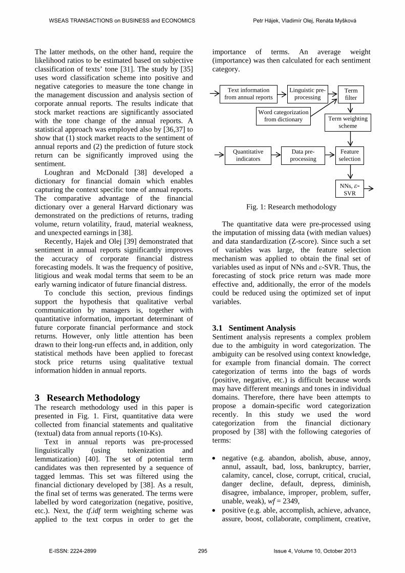
3 Research Methodology The research methodology used in this paper is presented in Fig. 1. First, quantitative data were collected from financial statements and qualitative (textual) data from annual reports (10-Ks).

Text in annual reports was pre-processed linguistically (using tokenization and lemmatization) [40]. The set of potential term candidates was then represented by a sequence of tagged lemmas. This set was filtered using the financial dictionary developed by [38]. As a result, the final set of terms was generated. The terms were labelled by word categorization (negative, positive, etc.). Next, the tf.idf term weighting scheme was applied to the text corpus in order to get the

importance of terms. An average weight (importance) was then calculated for each sentiment category.

Fig. 1: Research methodology

The quantitative data were pre-processed using the imputation of missing data (with median values) and data standardization (Z-score). Since such a set of variables was large, the feature selection mechanism was applied to obtain the final set of variables used as input of NNs and ε-SVR. Thus, the forecasting of stock price return was made more effective and, additionally, the error of the models could be reduced using the optimized set of input variables. 3.1 Sentiment Analysis Sentiment analysis represents a complex problem due to the ambiguity in word categorization. The ambiguity can be resolved using context knowledge, for example from financial domain. The correct categorization of terms into the bags of words (positive, negative, etc.) is difficult because words may have different meanings and tones in individual domains. Therefore, there have been attempts to propose a domain-specific word categorization recently. In this study we used the word categorization from the financial dictionary proposed by [38] with the following categories of terms: • negative (e.g. abandon, abolish, abuse, annoy,

annul, assault, bad, loss, bankruptcy, barrier, calamity, cancel, close, corrupt, critical, crucial, danger decline, default, depress, diminish, disagree, imbalance, improper, problem, suffer, unable, weak), wf = 2349,

• positive (e.g. able, accomplish, achieve, advance, assure, boost, collaborate, compliment, creative,

Text information from annual reports

Linguistic pre-processing

Term filter

Word categorization from dictionary Term weighting

scheme

Quantitative indicators

Data pre-processing

Feature selection

NNs, ε- SVR



delight, easy, enable, effective, enjoying, excellent, gain, progress, strong, succeed), wf = 354,

• uncertainty (e.g. ambiguity, assume, depend, crossroad, deviate, fluctuate, may, maybe, inexact, probably, random, reconsider, risk, unknown, variable), wf = 291,

• litigious (e.g. allege, amend, appeal, arbitrate, attest, attorney, bail, codified, constitution, contract, crime, court, defeasance, delegable, indict, judicial, legal, sue), wf = 871,

• modal strong (e.g. always, best, clearly, definitely, highest, must, never, strongly, undoubtedly), wf = 19,

• modal weak (e.g. almost, appeared, could, depend, might, nearly, possible, seldom, sometimes, suggest), wf = 27,

where wf is the frequency of terms in the word categories listed in the financial dictionary. The frequency of net positive words was determined as the positive term count minus the count for negation (positive terms can be easily qualified or compromised). The most common tf.idf (term frequency-inverse document frequency) term weighting scheme was used in this study. The weights can be defined as follows in the tf.idf

≥+

+=

otherwise 0

1 if log))log(1())log(1( ,

,i,j

i

ji

jitf

dfN

atf

w , (1)

where N denotes the total number of documents in the sample, dfi stands for the number of documents with at least one occurrence of the i-th term, tfi.j is the frequency of the i-th term in the j-th document, and a denotes the average term count in the document. 3.2 Feature Selection Algorithms that perform feature selection can generally be divided into two categories, the wrappers and the filters [41]. The wrappers use e.g. cross-validation in order to estimate the error of feature subsets. This approach may be slow since the predictor is called repeatedly. The filters operate independently of any learning algorithm. Undesirable features are filtered out of the data before prediction starts.

The original set of input parameters xmt, m=48

was optimized by using correlation based filter (CBF) [42]. The CBF optimizes the set of input parameters so that it evaluates the worth of a subset

of input parameters (features) by considering the individual predictive ability of each feature along with the degree of redundancy between them. The objective function f(λ), also known as Pearson’s correlation coefficient, is based on the heuristic that a good feature subset will have high correlation with the class label but will remain uncorrelated among themselves. Based on the states facts it is necessary to minimize the number of xm

t, m=48 and maximize function f(λ) which can be expressed as

f(λ)=rr

cr

ζλλλ

ζλ

××+

×

− )(1, (2)

where λ is the subset of features, ζcr is the average feature to output correlation, and ζrr is the average feature to feature correlation.

A genetic algorithm (GA) [43] was used to reduce the original set of input parameters xm

t, m=48 and, thus, to select only significant parameters. It was used as a search method for the mentioned feature selection method, i.e. it maximizes the objective function f(λ). It can be expressed for example in the following way: 1. Initialization: Let there be a random initial

population H. 2. Valuation: ∀λ∈Η calculate objective function

f(λ), the objective function states the quality of individual λ.

3. if λ

max f(λ)< ρ then repeat

/* ρ is the threshold value for objective function f(λ)*/

begin selection: random selection (1−ps)×P of individuals from the initial population H to the transitional population H’. The selection step reproduces genotypes based on their fitness function. /* ps is the probability of selection, P is the size of population */ crossing: probability selection pc×P/2 of pairs of individuals from the initial population H. For each pair create two descendants by crossing and add them to transitional population H’. /* pc is the probability of crossover */ mutation: invert random bits of individuals from the transitional population H’ with probability of mutation pm. actualization: H←H’. valuation: ∀λ∈Η calculate objective function f(λ) end 4. Return of individual λ∈Η, which takes the

highest value of objective function f(λ).



Based on the minimization of the number of parameters xm

t, m=48 using Pearson’s correlation coefficient and on the maximization of objective function f(λ) with defined parameters of the GA, it is possible to design a general formulation of the model. 3.3 Neural Networks The structure of MLP [44,45,46] is given by the task which it executes. The output of MLP can be expressed for example as follows

)( )(∑ ∑== =

K

1k

J

1j

tkj,kj,k dy xwv , (3)

where y is the output of the MLP, vk is the vector of synapses’ weights among neurons in the hidden layer and output neuron, wj,k is the vector of synapses’ weights among input neurons and neurons in the hidden layer, k is the index of neuron in the hidden layer, K is the number of neurons in the hidden layer, d is the activation function, j is the index of the input neuron, J is the number of the input neurons per one neuron in the hidden layer, and xj,k

t is the input vector of the MLP. In the process of learning, the values of synapse weights among neurons are adjusted. The most often used ones are gradient methods.

The term RBF NN [46,47] refers to any kind of feed-forward NN that uses RBF as their activation function. RBF NNs are based on supervised learning. The output f(x,H,w) RBF NN can be defined this way

∑=

×=q

1iii hwHf )()( xwx ,, ,

(4)

where H={h1(x),h2(x), … ,hi(x), … ,hq(x)} is a set of RBF activation functions of neurons in the hidden layer and wi are synapse weights. Each of the m components of the vector x=(x1,x2, … ,xk, … ,xm) is an input value for the q activation functions hi(x) of RBF neurons. The output f(x,H,w) of RBF NN represents a linear combination of outputs from q RBF neurons and corresponding synapse weights w.

The activation function hi(x) of an RBF NN in the hidden layer belongs to a special class of mathematical functions whose main characteristic is a monotonous rising or falling at an increasing distance from centre si of the activation function hi(x) of an RBF. Neurons in the hidden layer can use one of several activation functions hi(x) of an RBF NN, for example a Gaussian activation function (a one-dimensional activation function of RBF), a

rotary Gaussian activation function (a two-dimensional RBF activation function), multisquare and inverse multisquare activation functions or Cauchy’s functions. Results may be presented in this manner

h(x,S,R)= )(2||||

expi

i

r

sq

1i

−−∑

=

x, (5)

where x=(x1,x2, … ,xk, … ,xm) represents the input vector, S={s1,s2, … ,si, … ,sq} are the centres of activation functions hi(x) of RBF NN and R={r1,r2, … ,ri, … ,rq} are the radiuses of activation functions hi(x).

The neurons in the output layer represent only weighted sum of all inputs coming from the hidden layer. The activation function of neurons in the output layer can be linear, with the unit of the output eventually being converted by jump instruction to binary form.

The RBF NN learning process requires a number of centres si of activation function hi(x) of the RBF NNs networks to be set as well as for the most suitable positions for RBF centres si to be found. Other parameters are radiuses of centres si, rate of activation functions hi(x) of RBFs and synapse weights W(q,n). These are set up between the hidden and output layers. The design of an appropriate number of RBF neurons in the hidden layer is presented in [46,47]. Possibilities of centres recognition si are mentioned in [46,47] as a random choice. The position of the neurons is chosen randomly from a set of training data. This approach presumes that randomly picked centres si will sufficiently represent data entering the RBF NN. This method is suitable only for small sets of input data. Use on larger sets often results in a quick and needless increase in the number of RBF neurons in the hidden layer, and therefore unjustified complexity of the NN. The second approach to locating centres si of activation functions hi(x) of RBF neurons can be realized by a K-means algorithm. 3.4 Support Vector Regression In nonlinear regression ε-SVR [46,48,49,50] minimizes the loss function L(d,y) with insensitive ε [46,48,49]. Loss function L(d,y)= |d−y|, where d is the desired response and y is the output estimate. The construction of the ε-SVR for approximating the desired response d can be used for the extension of loss function L(d,y) as follows



ydydL −−=

0),( ε

ε elsefor ε≥− yd , (6)

where ε is a parameter. Loss function Lε(d,y) is called a loss function with insensitive ε.

Let the nonlinear regression model in which the dependence of the scalar d vector x expressed by d=f(x) + n. Additive noise n is statistically independent of the input vector x. The function f(.), and noise statistics are unknown. Next, let the sample training data (xi,di), i=1,2, ... ,N, where xi and di is the corresponding value of the output model d. The problem is to obtain an estimate of d, depending on x. For further progress is expected to estimate d, called y, which is widespread in the set of nonlinear basis functions ϕj(x), j=0,1, ... ,m1 this way

)()( xx ϕϕ Tm

0jjj wwy

1=∑=

=, (7)

where ϕ(x)=(ϕ0(x), ϕ1(x), … , ϕm1(x))T and

w=(w0,w1, ... ,wm1)T. It is assumed that ϕ0(x)=1 in

order to the weight w0 represents bias b. The solution to the problem is to minimize the empirical risk

),(1

ii

N

1iemp ydL

NR ∑=

=ε , (8)

under conditions of inequality ||w||2≤ c0, where c0 is a constant. The restricted optimization problem can be rephrased using two complementary sets of non-negative variables. Additional variables ξ and ξ´ describe loss function Lε(d,y) with insensitivity ε. The restricted optimization problem can be written as an equivalent to minimizing the cost functional

www TN

1i'iiC

2

1)(),,( )(' +∑ +=

=ξξξξφ , (9)

under the constraints of two complementary sets of non-negative variables ξ and ξ´. The constant C is a user-specified parameter. Optimization problem (9) can be easily solved in the dual form. The basic idea behind the formulation of the dual-shaped structure is the Lagrangian function [46], the objective function and restrictions. Can then be defined Lagrange multipliers with their functions and parameters which ensure optimality of these multipliers. The optimization of the Lagrangian function only describes the original regression problem. To formulate the corresponding dual problem a convex function can be obtained (for shorthand)

∑ ∑ −−== =

+−N

1i

N

1i'ii

'iii

'ii dQ )()(),( ααεαααα

∑ ∑= =

−−N

1i

N

1jji

'jj

'ii ,K )())((

2

1xxαααα , (10)

where K(xi,xj) is kernel function defined in accordance with Mercer's theorem [46,48,49]. Solving optimization problem is obtained by maximizing Q(α,α´) with respect to Lagrange multipliers α and α´ and provided a new set of constraints, which hereby incorporated constant C contained in the function definition φ(w,ξ,ξ´). Data points covered by the α ≠ α´, define support vectors [46,48,49]. 4 Dataset The indicators of fundamental analysis represent commonly used predictors of long-run stock market movement. Input variables used in our study for describing companies can be divided into two groups: (1) financial indicators and (2) sentiment indicators, see Table 1.

Only U.S. firms from the NASDAQ and New York Stock Exchange were selected. Quantitative financial indicators were drawn from the Value Line database, and sentiment indicators were drawn from annual reports available at U.S. Securities and Exchange Commission EDGAR System. All data were collected for the year t = 2010 and the stock price return was calculated as a one-year change (365 days after the release of the firms’ annual report). As a result, we were able to collect 685 data on U.S. firms.

In addition to the presented indicators, we also calculated their change over the last year (growth rate from 2009 to 2010), i.e. Δxi

t=(xit–xi

t-1)/xit-1,

where i=1,2, … ,24. Therefore, we used 48 input variables as the inputs of the optimization process (feature selection process).

As indicated in Table 1, several subgroups of financial indicators were used to control size (market capitalization), profitability, leverage, and market value ratios.

In general, the value of shares reflects the authentic data obtained from the analysis of previous years and the expected data based on the estimates of future development. According to the efficient market theory the changes in the market price of securities are represented by random variables. The prices are the result of supply and demand responding to price-sensitive information [51]. Methods for assessing the investment criteria



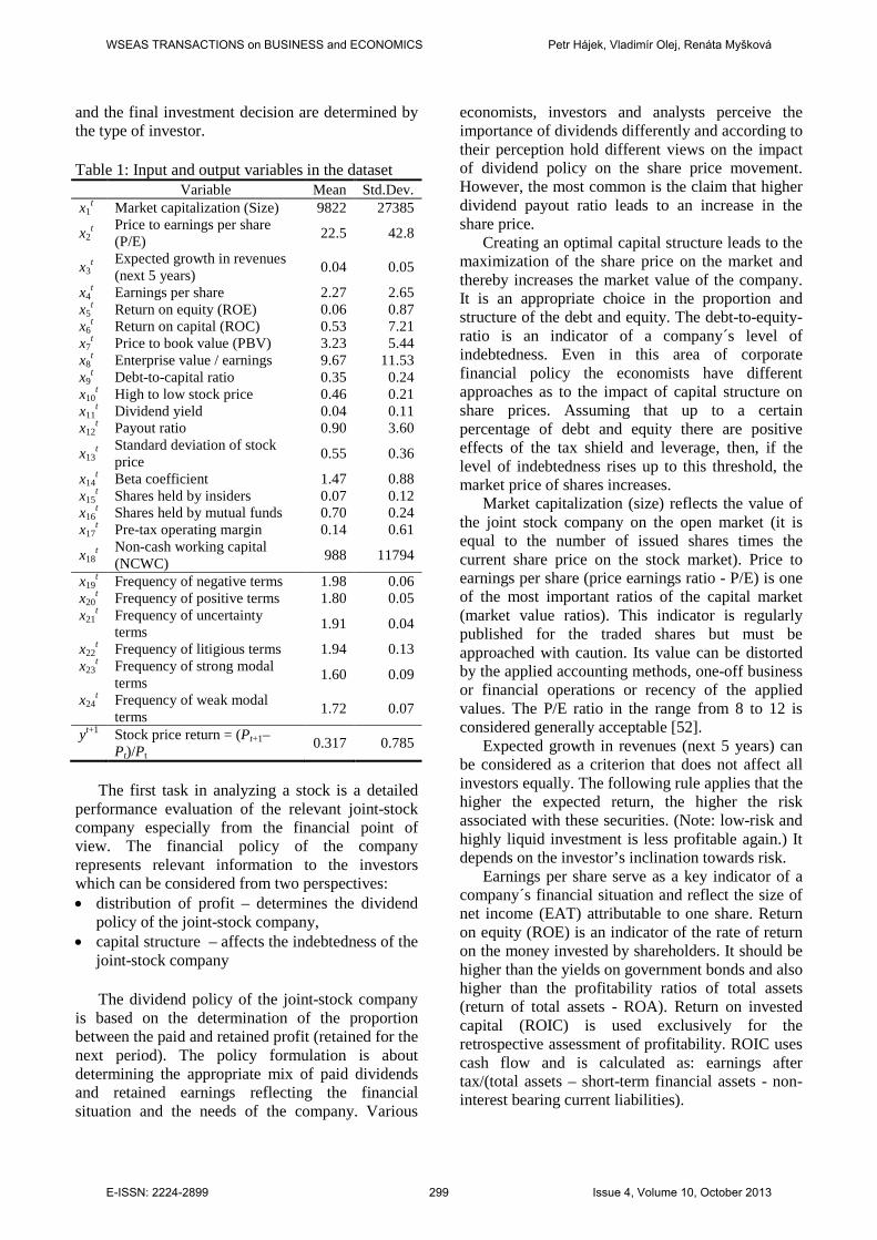
and the final investment decision are determined by the type of investor. Table 1: Input and output variables in the dataset Variable Mean Std.Dev. x1

t Market capitalization (Size) 9822 27385

x2t Price to earnings per share

(P/E) 22.5 42.8

x3t Expected growth in revenues

(next 5 years) 0.04 0.05

x4t Earnings per share 2.27 2.65

x5t Return on equity (ROE) 0.06 0.87

x6t Return on capital (ROC) 0.53 7.21

x7t Price to book value (PBV) 3.23 5.44

x8t Enterprise value / earnings 9.67 11.53

x9t Debt-to-capital ratio 0.35 0.24

x10t High to low stock price 0.46 0.21

x11t Dividend yield 0.04 0.11

x12t Payout ratio 0.90 3.60

x13t Standard deviation of stock

price 0.55 0.36

x14t Beta coefficient 1.47 0.88

x15t Shares held by insiders 0.07 0.12

x16t Shares held by mutual funds 0.70 0.24

x17t Pre-tax operating margin 0.14 0.61

x18t Non-cash working capital

(NCWC) 988 11794

x19t Frequency of negative terms 1.98 0.06

x20t Frequency of positive terms 1.80 0.05

x21t Frequency of uncertainty

terms 1.91 0.04

x22t Frequency of litigious terms 1.94 0.13

x23t Frequency of strong modal

terms 1.60 0.09

x24t Frequency of weak modal

terms 1.72 0.07

yt+1 Stock price return = (Pt+1–Pt)/Pt

0.317 0.785

The first task in analyzing a stock is a detailed

performance evaluation of the relevant joint-stock company especially from the financial point of view. The financial policy of the company represents relevant information to the investors which can be considered from two perspectives: • distribution of profit – determines the dividend

policy of the joint-stock company, • capital structure – affects the indebtedness of the

joint-stock company

The dividend policy of the joint-stock company is based on the determination of the proportion between the paid and retained profit (retained for the next period). The policy formulation is about determining the appropriate mix of paid dividends and retained earnings reflecting the financial situation and the needs of the company. Various

economists, investors and analysts perceive the importance of dividends differently and according to their perception hold different views on the impact of dividend policy on the share price movement. However, the most common is the claim that higher dividend payout ratio leads to an increase in the share price.

Creating an optimal capital structure leads to the maximization of the share price on the market and thereby increases the market value of the company. It is an appropriate choice in the proportion and structure of the debt and equity. The debt-to-equity-ratio is an indicator of a company´s level of indebtedness. Even in this area of corporate financial policy the economists have different approaches as to the impact of capital structure on share prices. Assuming that up to a certain percentage of debt and equity there are positive effects of the tax shield and leverage, then, if the level of indebtedness rises up to this threshold, the market price of shares increases.

Market capitalization (size) reflects the value of the joint stock company on the open market (it is equal to the number of issued shares times the current share price on the stock market). Price to earnings per share (price earnings ratio - P/E) is one of the most important ratios of the capital market (market value ratios). This indicator is regularly published for the traded shares but must be approached with caution. Its value can be distorted by the applied accounting methods, one-off business or financial operations or recency of the applied values. The P/E ratio in the range from 8 to 12 is considered generally acceptable [52].

Expected growth in revenues (next 5 years) can be considered as a criterion that does not affect all investors equally. The following rule applies that the higher the expected return, the higher the risk associated with these securities. (Note: low-risk and highly liquid investment is less profitable again.) It depends on the investor’s inclination towards risk.

Earnings per share serve as a key indicator of a company´s financial situation and reflect the size of net income (EAT) attributable to one share. Return on equity (ROE) is an indicator of the rate of return on the money invested by shareholders. It should be higher than the yields on government bonds and also higher than the profitability ratios of total assets (return of total assets - ROA). Return on invested capital (ROIC) is used exclusively for the retrospective assessment of profitability. ROIC uses cash flow and is calculated as: earnings after tax/(total assets – short-term financial assets - non-interest bearing current liabilities).



Price to book value – P/B (Price/Book Value Ratio) is the ratio of the share market value to its book value. A positive aspect of this indicator is that it takes into account equity (not just profits), but on the other hand it is influenced by accounting practices, which can distort the indicator in the inter-company comparison process. The market price of shares in a prosperous company exceeds their book value, so the P/B ratio should be greater than 1.

Book value per share - the ratio of equity to the number of common shares – it should show a growing tendency in case of thriving businesses. Debt-to-capital ratio is the ratio of the company's debt to its total capital, so by the debt proportion it is possible to assess whether the company is more or less likely to use debt financing. The optimal debt ratio is different for different business sectors and depends on the investment demands of the particular business. 50-60% share of debt on total assets of the company is considered as an optimal limit.

High to low stock price ('52-Week High / Low ') - the highest and lowest prices at which the shares are traded at in the previous year (in the last 52 weeks). It does not only serve the investors to predict the future movement of prices but also the owners to decide when to buy or sell the shares.

Dividend payout ratio expresses the proportion of disposable (net) income paid to shareholders in dividends. The ratio´s amount should not be the only assessed value – if a company operates in a purely investment-oriented industry, this ratio decreases, but in the long run particularly these investments lead to the growth of share prices.

Dividend yield measures the value of the dividend per share to its current price. It is necessary to take into account that the dividend is backdated, while the share price is up to date.

The standard deviation of stock price - the statistical value is used to express the historical volatility. The greater the standard deviation, the greater the stock price volatility expected by the investors in the future. (e.g. the standard deviation of a stable blue chip stock will be low).

Beta coefficient expresses the correlation between the security returns (or the industry) and returns of the market portfolio represented by the market index in a specified time period. Beta coefficient reflects the extent to which the particular security is subject to the influence of the general market rises or falls, and measures the contribution of the security to the risk of the portfolio. Stocks with a beta greater than 1 indicate risky securities because they tend to intensify the general stock market movements. In the long run, the beta

coefficient is usually higher in companies with a lower market capitalization than in those with a larger market capitalization.

Shares held by insiders - percentage of the company´s outstanding shares, employee shares – The legislation for the employee share ownership differs in each country. In most countries, employee shares usually do not constitute any voting rights and are not freely tradable (restricted stock unit). They are granted to employees, for example as a form of compensation.

Shares held by mutual funds - shares in investment funds - this indicator is important for assessing the amount of shares held by investment funds. In the event that the funds announce the intention to reduce shares in the company, it can cause a sharp increase in profit taking on the title to shares (sale of shares). This may cause their prices to fall.

Other indicators can be also used to assess the financial results and value of the company. Table 1 also includes: • Pre-tax operating margin - the profit margin

before taxes - the ratio of profits before interest and tax to revenues,

• Non-cash working capital (NCWC) – is expressed as the sum of inventory and receivables. The amount is determined with regard to the nature of the business on the basis of past business development and experience of managers. In addition to these indicators, the interest and

expectations of investors may also be affected by the way the company presents itself. Given the large amount of information contained in the annual report other aspects are checked in this mandatory document. The legislation usually regulates the particulars in the annual report that have to be stated unconditionally, the other stated data depend on the management of the company. This means that with the same financial results the report may be written in different ways - optimistic or pessimistic. A more cautious management is rather critical; a management which is able to accept a higher level of risk assesses the results more generously.

As shown in previous literature, sentiment indicators are strongly related to financial indicators and, additionally, they also inform on the business position (business diversification, business risk, character, organizational problems, management evaluation, accounting quality, etc.).

Since the number of input variables was too large and the impact of many variables on stock price return is ambiguous, respectively, we performed the



process of feature selection using the CBF method. This step reduces the dimenstionality of the feature space, makes the operation of learning algorithms faster, and may also improve the forecasting accuracy.

A GA was used as a search method for the CBF in the stage of feature selection. The parameters of the GA were set as follows: the propability of crossover pc =0.8, the probability of mutation pm=0.03, the maximum number of generations=40, population size (feature sets)=20. The found set of variables is presented in Table 2. In the optimum set of variables, there were P/E ratio, expected growth in revenues, ROC, and high to low stock price. In addition to previous years’ absolute values of these indicators, dynamic indicators such as ΔROE or ΔNCWC played an important role in stock price return forecasting. Furthermore, the change of sentiment (negative and uncertainty) seems to be an important determinant too.

Table 2: Input and output variables after the optimization

Variable x2

t Price to earnings per share x3

t Expected growth in revenues (next 5 years) Δx3

t Δ Expected growth in revenues (next 5 years) Δx5

t Δ Return on equity x6

t Return on capital x10

t High to low stock price Δx17

t Δ Pre-tax operating margin Δx18

t Δ Non-cash working capital Δx19

t Δ Frequency of negative terms Δx21

t Δ Frequency of uncertainty terms yt+1 Stock price return = (Pt+1–Pt)/Pt

5 Experimental Results For the experiments, data were divided into 5 parts of the same size and then trained with 4 parts (80%) and tested with 1 remaining part (20%). This procedure was repeated 5 times for all parts. In the results, we refer to average errors over the 5 experiments. We compared the results obtained using NNs (MLP and RBF) and ε-SVR measuring the MSE (mean squared error) and R2 (coefficient of determination).

Since the results of NNs and ε-SVR are sensitive to the setting of learning parameters we automatically determined their values in the following way.

First, MLPs and RBF NNs were employed to forecast the stock price return. The MLP model was trained using conjugate gradient method with 10000 maximum iterations. Logistic activation functions

were used in the hidden layer, and linear activation functions in the output layer. The number of neurons (showing on the complexity of the MLP model) in one hidden layer was set from the set k={2,3, … ,20}.

The parameters of the RBF model were determined automatically using a GA. The number of neurons in the hidden layer was chosen from the set si∈{1,2, … ,100}, the radius 1/ri of RBF from <0.01,400> and regularization parameter lambda from <0.001,10>. The employed GA worked with the population size of 200 and the maximum number of generations=20. Finally, we compared the forecasting results with a linear regression model (Table 3). Table 3: Forecasting performance of the NNs Method MSE R2 MLP (# neurons=8) 0.099 0.318 RBF NNs (# neurons=8) 0.106 0.131 Linear regression 0.110 0.154

We also investigated the importance of the input

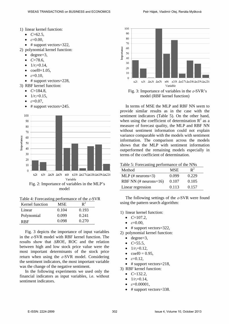
variables in the NNs’ models. The importance was obtained by the evaluation of input variables’ effects on the forecasting results. In this study the calculation of input variables’ importance was performed using sensitivity analysis. The values of each of the input variables were randomized and the effect on the MSE of the model was measured. Finally the contributions of input variables were standardized so that the contribution of the most important input variable was 100%, and the contributions of other input variables were related to the most important variable. Thus, the resulting contributions of the input variables represent relative importance values. The importance of the variables in the MLP’s model is presented in Fig. 2. The results show that ΔROE, the relation between high and low stock price value, and ΔNCWC were the most important determinants of the stock price return. The results also indicate that sentiment information is a more important determinant compared to the ε-SVR model (Fig. 3).

The ε-SVR algorithm was trained with linear, polynomial (degree=3) and RBF kernel functions (Table 4). The RBF kernel function proved to be the most appropriate for the prediction. Complexity parameter C was chosen from the interval <0.1,50000> and 1/ri from <0.01,20> using pattern search algorithm, see e.g. [53].

The following settings were found with the pattern search algorithm:



1) linear kernel function: • C=62.5, • ε=0.00, • # support vectors=322,

2) polynomial kernel function: • degree=3, • C=78.6, • 1/ri=0.14, • coef0=1.05, • ε=0.10, • # support vectors=228,

3) RBF kernel function: • C=184.8, • 1/ri=0.15, • ε=0.07, • # support vectors=245.

Fig. 2: Importance of variables in the MLP’s

model

Table 4: Forecasting performance of the ε-SVR Kernel function MSE R2 Linear 0.104 0.193 Polynomial 0.099 0.241 RBF 0.098 0.270

Fig. 3 depicts the importance of input variables

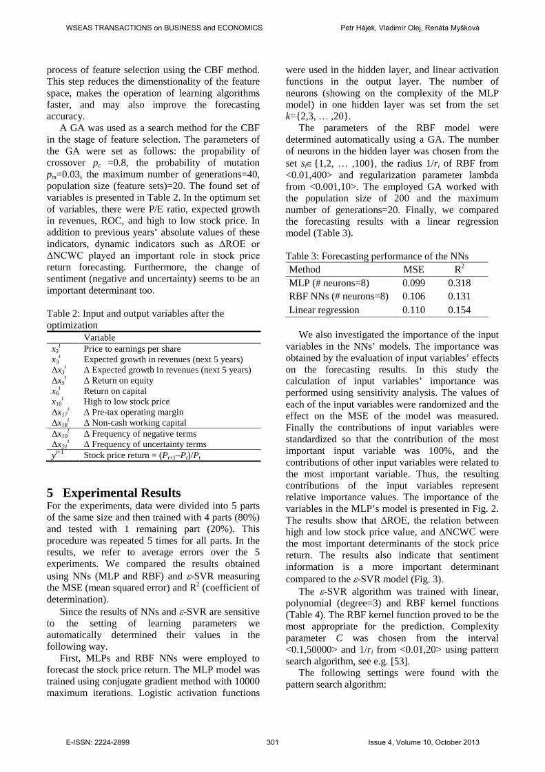
in the ε-SVR model with RBF kernel function. The results show that ΔROE, ROC and the relation between high and low stock price value were the most important determinants of the stock price return when using the ε-SVR model. Considering the sentiment indicators, the most important variable was the change of the negative sentiment.

In the following experiments we used only the financial indicators as input variables, i.e. without sentiment indicators.

Fig. 3: Importance of variables in the ε-SVR’s

model (RBF kernel function)

In terms of MSE the MLP and RBF NN seem to provide similar results as in the case with the sentiment indicators (Table 5). On the other hand, when using the coefficient of determination R2 as a measure of forecast quality, the MLP and RBF NN without sentiment information could not explain variance comparable with the models with sentiment information. The comparison across the models shows that the MLP with sentiment information outperformed the remaining models especially in terms of the coefficient of determination. Table 5: Forecasting performance of the NNs Method MSE R2 MLP (# neurons=3) 0.099 0.229 RBF NN (# neurons=16) 0.107 0.105 Linear regression 0.113 0.157

The following settings of the ε-SVR were found

using the pattern search algorithm: 1) linear kernel function:

• C=107.2, • ε=0.00, • # support vectors=322,

2) polynomial kernel function: • degree=3, • C=55.5, • 1/ri=0.12, • coef0 = 0.95, • ε=0.12, • # support vectors=218,

3) RBF kernel function: • C=132.2, • 1/ri=0.14, • ε=0.00001, • # support vectors=338.



The same facts as for the MLP and RBF NN models hold also true for the ε-SVR models (see Table 6).

Table 6: Forecasting performance of the ε-SVR Kernel function MSE R2 Linear 0.100 0.208 Polynomial 0.099 0.212 RBF 0.103 0.182

6 Conclusion The article presents a stock price forecasting model that combines financial indicators with the indicators obtained from the textual annual reports of firms. The sentiment indicators covered six categories of sentiment. We hypothesised that the prediction of stock price return can be more accurate when using the qualitative textual information hidden in the annual reports. The findings from this study make several contributions to the current literature. First, we conclude that larger variance in the next year’s stock price return can be explained using the change in annual reports’ sentiment, specifically in the categories of negative and uncertain terms. Second, surprisingly, it was not the sentiment (tone) of the annual report itself, but the change in the sentiment that was the most important determinant in the models. In addition to the change of sentiment, the long-run stock price returns were particularly affected by profitability ratios and fundamental analysis indicators. ε-SVRs and NNs performed better than linear regression models when considering the sentiment information. This suggests that ε-SVRs and NNs better coped with the growing complexity of the forecasting problem which is line with previous literature, e.g. [54,55].

The development of share prices is influenced not only by the mentioned factors but also by the possibilities and intentions of investors. The possibility of investment is determined by the size of the initial investment, which is different for each type of investment. Other decisions relate to the intention of the investor to choose either direct or indirect investments. Direct investments are of strategic nature and their purpose from the investor´s point of view is to acquire the majority stake in the company and take over the control and thus be able to exercise the rights associated with an investment in a particular security. Indirect investments are portfolio investments designed to diversify risk and thus eliminate losses. The percentage share of an investor in the company's assets in case of indirect investments is significantly

smaller than in case of direct investments (up to 10% of the issued capital). The decision making process of investors is also affected by the situation on the stock market. This situation is related to the development of macroeconomic variables, namely to the growth of gross domestic product, the business cycle and fiscal policy, inflation and interest rates, money supply and the volume of foreign capital.

The study has gone some way towards enhancing our understanding of stock market behaviour. However, further important limitations need to be considered. The current investigation was limited to the U.S. stock market and to a short time period. Therefore, the approach proposed in this study may be applied to other stock markets (and derivative markets [56]) elsewhere in the world and to a longer time period. Thus, country-specific and time-specific determinants may be taken into account. Another limitation consists in the fact that the words in the word categories may have various importances for stock price return prediction. Thus, the accuracy improvement of the models may be limited. A further study with more focus on statistical approach is therefore suggested. Finally,

The experiments in this study were carried out in Weka 3.6.5 and DTREG in MS Windows 7 operation system. Acknowledgment This work was supported by the scientific research project of the Czech Sciences Foundation Grant No: 13-10331S. References: [1] S.J. Grossman, R.J. Shiller, The Determinants

of the Variability of Stock Market Prices, The American Economic Review, Vol.71, No.2, 1981, pp. 222–227.

[2] K. Michalak, P. Lipinski, Prediction of High Increases in Stock Prices using Neural Networks, Neural Network World, Vol.15, 2005, pp. 359–366.

[3] K.J. Kim, Financial Time Series Forecasting using Support Vector Machines, Neurocomputing, Vol.55, 2003, pp. 307–319.

[4] G. Zhang, B.E. Patuwo, M.Y. Hu, Forecasting with Artificial Neural Networks: The State of the Art, International Journal of Forecasting, Vol.14, 1998, pp. 35–62.

[5] Y. Yoon, J. Swales, Prediction Stock Price Performance: A Neural Network Approach, In: Proc. of the 24th Annual Hawaii Int. Conf. on System Science, 1991, pp.156–162.



[6] J. Yao, H.L. Poh, Forecasting the KLSE Index using Neural Networks, In: Proc. of the IEEE Int. Conf. on Neural Networks, Vol.2, 1995, pp. 1012–1017.

[7] N. Baba, M. Kozaki, An Intelligent Forecasting System of Stock Price using Neural Networks, In: Proc. of the Int. Joint Conf. on Neural Networks, Vol.1, 1992, pp. 371–377.

[8] J.H. Choi, M.K. Lee, M.W. Rhee, Trading S&P 500 Stock Index Futures using a Neural Network, In: Proc. of the Annual Int. Conf. on Artificial Intelligence Applications on Wall Street, New York, 1995, pp. 63–72.

[9] D. Enke, S. Thawornwong, The Use of Data Mining and Neural Networks for Forecasting Stock Market Returns, Expert Systems with Applications, Vol.29, No.4, 2005, pp. 927–940.

[10] X.B. Yan, Z. Wang, S. Yu, Y. Li, Time Series Forecasting with RBF Neural Network, In: Proc. of the 4th Int. Conf. on Machine Learning and Cybernetics, Guangzhou, Vol.8, 2005, pp.4680–4683.

[11] K. Chen, H. Lin, T. Huang, The Prediction of Taiwan 10-year Government Bond Yield, WSEAS Transactions on Systems, Vol.8, No.9, 2009, pp. 1051–1060.

[12] L.J. Cao , F.E.H. Tay, Support Vector Machine with Adaptive Parameters in Financial Time Series Forecasting, IEEE Transactions on Neural Networks, Vol.14, No.6, 2003, pp. 1506–1518.

[13] Ch.K. Volos, I.M. Kyprianidis, S.G. Stavrinides, I.N. Stouboulos, L. Magafas, A.N. Anagnostopoulos, Nonlinear Financial Dynamics from an Engineer’s Point of View, Journal of Engineering Science and Technology Review, Vol.4, 2011, pp. 281–285.

[14] Ch.K. Volos, I.M. Kyprianidis, S.G. Stavrinides, I.N. Stouboulos, Synchronization Phenomena in Coupled Nonlinear Systems Applied in Economic Cycles, WSEAS Transactions on Systems, Vol.11, No.12, 2012, pp. 681–690.

[15] F. Neri, Learning Predictive Models for Financial Time Series by Using Agent Based Simulations, Lecture Notes in Computer Science, Vol.7190, 2012, pp. 202–221.

[16] F. Neri, Agent based Modeling under Partial and Full Knowledge Learning Settings to Simulate Financial Markets, AI Communications, Issue 4, Vol.25, 2012, pp. 295–304.

[17] P.Ch. Chang, Ch.H. Liu, A TSK Type Fuzzy Rule based System for Stock Price Prediction,

Expert Systems with Applications, Vol.34, No.1, 2008, pp. 135–144.

[18] R. Tsaih, Y. Hsu, C.C. Lai, Forecasting S&P 500 Stock Index Futures with a Hybrid AI System, Decision Support Systems, Vol.23, No.2, 1998, pp. 161–174.

[19] G. Armano, M. Marchesi, A. Murru, A Hybrid Genetic-Neural Architecture for Stock Indexes Forecasting, Information Science, Vol.170, No.1, 2005, pp. 3–33.

[20] V. Olej, Prediction of the Index Fund by Takagi-Sugeno Fuzzy Inference Systems and Feed-Forward Neural Network, In: Proc. of the 5th WSEAS Int. Conf. on Artificial Intelligence, Knowledge Engineering and Data Bases, Madrid, Spain, 2006, pp. 7–12.

[21] R.K. Lai, Ch.Y. Fan, W.H. Huang, P.Ch. Chang, Evolving and Clustering Fuzzy Decision Tree for Financial Time Series Data Forecasting, Expert Systems with Applications, Vol.36, 2009, pp. 3761–3773.

[22] P. Hajek, Forecasting Stock Market Trend using Prototype Generation Classifiers, WSEAS Transactions on Systems, Vol.11, No.11, 2012, pp. 671–680.

[23] J.Y. Campbell, J. Ammer, What Moves the Stock and Bond Markets? A Variance Decomposition for Long-Term Asset Returns, The Journal of Finance, Vol.48, No.1, 1993, pp. 3–37.

[24] J.Y. Campbell, Y. Hamao, Predictable Stock Returns in the United States and Japan: A Study of Long-term Capital Market Integration, The Journal of Finance, Vol.47, No.1, 1992, pp. 43–69.

[25] J.Y. Campbell, R.J. Shiller, Valuation Ratios and the Long-run Stock Market Outlook: An Update. No.w8221, National Bureau of Economic Research, 2001.

[26] Z. Ding, C.W.J. Granger, R.F. Engle, A Long Memory Property of Stock Market Returns and a New Model, Journal of Empirical Finance, Vol.1, No.1, 1993, pp. 83–106.

[27] P. Bak, M. Paczuski, M. Shubik, Price Variations in a Stock Market with Many Agents, Physica A: Statistical Mechanics and its Applications, Vol.246, No.3, 1997, pp. 430–453.

[28] N. Barberis, A. Shleifer, R. Vishny, A Model of Investor Sentiment, Journal of Financial Economics, Vol.49, No.3, 1998, pp. 307–343.

[29] F. Neri, Quantitative Estimation of Market Sentiment: A Discussion of Two Alternatives, WSEAS Transactions on Systems, Vol.11, No.12, 2012, pp. 691–702.



[30] J. Bollen, H. Mao, X. Zeng, Twitter Mood Predicts the Stock Market, Journal of Computational Science, Vol.2, No.1, 2011, pp. 1–8.

[31] P.C. Tetlock, Giving Content to Investor Sentiment: The Role of Media in the Stock Market, Journal of Finance, Vol.62, 2007, pp. 1139–1168.

[32] E.A. Demers, C. Vega, Soft Information in Earnings Announcements: News or Noise? Working Paper, INSEAD, 2010.

[33] S. Das, M. Chen, Yahoo! for Amazon: Opinion Extraction from Small Talk on the Web. Working Paper, Santa Clara University, 2001.

[34] G.F. Kohut, A.H. Segars, The President's Letter to Stockholders: An Examination of Corporate Communication Strategy, Journal of Business Communication, Vol.29, No.1, 1992, pp. 7–21.

[35] R. Feldman, S. Govindaraj et al., Management's Tone Change, Post Earnings Announcement Drift and Accruals, Review of Accounting Studies, Vol.15, 2010, pp.915–953.

[36] F. Li, The Information Content of Forward-Looking Statements in Corporate Filings - A Naïve Bayesian Machine Learning Approach, Journal of Accounting Research, Vol.48, No.5, 2010, pp. 1049–1102.

[37] A. Huang, A. Zang et al., Informativeness of Text in Analyst Reports: A Naïve Bayesian Machine Learning Approach. Working Paper, The Hong Kong University of Science and Technology, 2010.

[38] T. Loughran, B. McDonald, When Is a Liability Not a Liability? Textual Analysis, Dictionaries, and 10-Ks, The Journal of Finance, Vol.66, No.1, 2011, pp. 35–65.

[39] P. Hajek, V. Olej, Evaluating Sentiment in Annual Reports for Financial Distress Prediction using Neural Networks and Support Vector Machines. In: Proc. of the 14th Engineering Applications of Neural Networks (EANN’13), 2013, (in press).

[40] R. Feldman, M. Fresko et al., Text Mining at the Term Level. In: Proc. of the 2nd Europ. Symposium on Principles of Data Mining and Knowledge Discovery, 1998, pp. 65–73.

[41] G.H. John, R. Kohavi, K. Pfleger, Irrelevant Features and the Subset Selection Problem. In: Proc. of the 11th Int. Conf. on Machine Learning, 1994, pp. 121–129.

[42] M.A. Hall, Correlation-Based Feature Subset Selection for Machine Learning. Hamilton, University of Waikato, 1998.

[43] S. N. Sivananda, S. N. Deepa, Introduction to Genetic Algorithms. Berlin, Springer Verlag, 2007.

[44] R.P. Lippman, An Introduction to Computing with Neural Nets, IEEE ASSP Mag., Vol.4, 1987, pp. 4–22.

[45] F. Rosenblatt, The Perceptron, a Probabilistic Model for Information Storage and Organization in the Brain, Psychol. Rev., Vol.65, No.6, 1958, pp. 386–408.

[46] S. Haykin, Neural Networks: A Comprehensive Foundation. New Jersey, Prentice-Hall Inc., 1999.

[47] D.S. Broomhead, D. Lowe, Multivariate Functional Interpolation and Adaptive Networks, Complex Systems, Vol.2, 1988, pp. 321–355.

[48] N. Cristianini, J. Shawe-Taylor, An Introduction to Support Vector Machines and other Kernel-based Learning Methods. Cambridge University Press, 2000.

[49] A. Smola, J. Scholkopf, A Tutorial on Support Vector Regression, Statistics and Computing, Vol.14, 2004, pp. 199–222.

[50] V.N. Vapnik, The Nature of Statistical Learning Theory. Springer, New York, 1995.

[51] P. Duspiva, J. Novotný, Utilization of Quantitative Methods in the Decision Making Process of a Manager. Scientific Papers of the University of Pardubice, Vol.17, No.2, 2010, pp. 63–69.

[52] O. Rejnuš, Finanční Trhy. Key Publishing, Ostrava, 2011, (in Czech).

[53] P. Hajek, V. Olej, Credit Rating Modelling by Kernel-based Approaches with Supervised and Semi-Supervised Learning, Neural Computing & Applications, Vol.20, No.6, 2011, pp. 761–773.

[54] H. Lin, K. Chen, Soft Computing Algorithms in Price of Taiwan Real Estates, WSEAS Transactions on Systems, Vol.10, No.10, 2011, pp. 342–351.

[55] P. Hajek, V. Olej, Municipal Revenue Prediction by Ensembles of Neural Networks and Support Vector Machines, WSEAS Transactions on Computers, Vol.9, No.11, 2010, pp. 1255–1264.

[56] K. Chang, S.S. Wang, P. Ke, Y.R. Huang, Y. Zhen, The Valuation of Futures Options for Emissions Allowances under the Term Structure of Stochastic Multi-Factors, WSEAS Transactions on Systems, Vol.11, No.12, 2012, pp. 661–670.



forecasting stock prices using sentiment information … · forecasting stock prices using...

Documents