forecasting the stock market index using artificial intelligence … · 2016-06-14 · forecasting...
TRANSCRIPT
Forecasting the Stock Market Index
Using Artificial Intelligence Techniques
Lufuno Ronald Marwala
A dissertation submitted to the Faculty of Engineering and the Built Environment, University of the
Witwatersrand, Johannesburg, in fulfilment of the requirements for the degree of Master of Science
in Engineering.
Johannesburg,

Declaration
I declare that this dissertation is my own, unaided work, except where otherwise acknowledged.
It is being submitted for the degree of Master of Science in Engineering in the University of the
Witwatersrand, Johannesburg. It has not been submitted before for any degree or examination in
any other university.
Signed this day of 20
Lufuno Ronald Marwala
i
Abstract
The weak form of Efficient Market hypothesis (EMH) states that it is impossible to forecast the future
price of an asset based on the information contained in the historical prices of an asset. This means
that the market behaves as a random walk and as a result makes forecasting impossible. Furthermore,
financial forecasting is a difficult task due to the intrinsic complexity of the financial system. The
objective of this work was to use artificial intelligence (AI) techniques to model and predict the future
price of a stock market index. Three artificial intelligence techniques, namely, neural networks (NN),
support vector machines and neuro-fuzzy systems are implemented in forecasting the future price of
a stock market index based on its historical price information. Artificial intelligence techniques have
the ability to take into consideration financial system complexities and they are used as financial
time series forecasting tools. Two techniques are used to benchmark the AI techniques, namely,
Autoregressive Moving Average (ARMA) which is linear modelling technique and random walk (RW)
technique. The experimentation was performed on data obtained from the Johannesburg Stock
Exchange. The data used was a series of past closing prices of the All Share Index. The results
showed that the three techniques have the ability to predict the future price of the Index with
an acceptable accuracy. All three artificial intelligence techniques outperformed the linear model.
However, the random walk method outperfomed all the other techniques. These techniques show an
ability to predict the future price however, because of the transaction costs of trading in the market,
it is not possible to show that the three techniques can disprove the weak form of market efficiency.
The results show that the ranking of performances support vector machines, neuro-fuzzy systems,
multilayer perceptron neural networks is dependent on the accuracy measure used.
ii

To my family and Busisiwe
iii

Acknowledgements
I wish to thank Professor Snadon, Mr Ian Campbell and Professor Brian Wigdorowitz for their
supervision. I would also like to thank my family for all the support they have given me throughout
my studies. I would also like to thank Busisiwe for believing in me.
iv

Contents
Declaration i
Abstract ii
Acknowledgements iv
Contents v
List of Figures xii
List of Tables xvii
Nomenclature xviii
1 Introduction 1
1.1 Classification vs. Regression . . . . . . . . . . . . . . . . . . . . . . . . . . . . . . . . . 2
1.2 Motivation . . . . . . . . . . . . . . . . . . . . . . . . . . . . . . . . . . . . . . . . . . 3
1.3 Research Hypotheses . . . . . . . . . . . . . . . . . . . . . . . . . . . . . . . . . . . . . 3
1.4 Objective of the Report . . . . . . . . . . . . . . . . . . . . . . . . . . . . . . . . . . . 3
1.5 Structure of the Report . . . . . . . . . . . . . . . . . . . . . . . . . . . . . . . . . . . 4
2 Forecasting 5
v

CONTENTS
2.1 Introduction . . . . . . . . . . . . . . . . . . . . . . . . . . . . . . . . . . . . . . . . . . 5
2.2 Criteria selection and comparison of forecasting methods . . . . . . . . . . . . . . . . . 5
2.2.1 Accuracy . . . . . . . . . . . . . . . . . . . . . . . . . . . . . . . . . . . . . . . 6
2.2.2 Pattern of the data and its effects on individual forecasting methods . . . . . . 6
2.2.3 Time horizon effects on forecasting methods . . . . . . . . . . . . . . . . . . . . 6
2.2.4 Ease of Application . . . . . . . . . . . . . . . . . . . . . . . . . . . . . . . . . 7
2.3 Accuracy measure selection . . . . . . . . . . . . . . . . . . . . . . . . . . . . . . . . . 7
2.4 In-sample versus out-of-sample evaluation . . . . . . . . . . . . . . . . . . . . . . . . . 8
2.5 Transaction costs and forecasting . . . . . . . . . . . . . . . . . . . . . . . . . . . . . . 8
2.6 Forecasting studies . . . . . . . . . . . . . . . . . . . . . . . . . . . . . . . . . . . . . . 9
3 The market 11
3.1 Johannesburg Stock Exchange . . . . . . . . . . . . . . . . . . . . . . . . . . . . . . . . 11
3.1.1 What is Market index? . . . . . . . . . . . . . . . . . . . . . . . . . . . . . . . 11
3.2 Efficient Market Hypothesis . . . . . . . . . . . . . . . . . . . . . . . . . . . . . . . . . 12
3.2.1 Studies evaluating EMH . . . . . . . . . . . . . . . . . . . . . . . . . . . . . . . 14
3.3 Modelling stock prices or return . . . . . . . . . . . . . . . . . . . . . . . . . . . . . . . 15
3.3.1 Previous techniques . . . . . . . . . . . . . . . . . . . . . . . . . . . . . . . . . 15
3.3.2 Techniques based on mathematics . . . . . . . . . . . . . . . . . . . . . . . . . 16
3.4 South African studies . . . . . . . . . . . . . . . . . . . . . . . . . . . . . . . . . . . . 18
4 Artificial intelligence techniques 20
4.1 Neural networks . . . . . . . . . . . . . . . . . . . . . . . . . . . . . . . . . . . . . . . 20
4.1.1 Network topologies . . . . . . . . . . . . . . . . . . . . . . . . . . . . . . . . . . 22
vi
CONTENTS
4.1.2 Multi-layer perceptron . . . . . . . . . . . . . . . . . . . . . . . . . . . . . . . . 22
4.1.3 Network training . . . . . . . . . . . . . . . . . . . . . . . . . . . . . . . . . . . 26
4.1.4 Radial basis function network . . . . . . . . . . . . . . . . . . . . . . . . . . . . 27
4.2 Support vector machines . . . . . . . . . . . . . . . . . . . . . . . . . . . . . . . . . . . 30
4.2.1 Support vector machines classification . . . . . . . . . . . . . . . . . . . . . . . 31
4.2.2 Support vector regression . . . . . . . . . . . . . . . . . . . . . . . . . . . . . . 32
4.2.3 SVM in a nutshell . . . . . . . . . . . . . . . . . . . . . . . . . . . . . . . . . . 36
4.3 Neuro-fuzzy models . . . . . . . . . . . . . . . . . . . . . . . . . . . . . . . . . . . . . . 38
4.3.1 Fuzzy Systems . . . . . . . . . . . . . . . . . . . . . . . . . . . . . . . . . . . . 38
4.3.2 Mamdani models . . . . . . . . . . . . . . . . . . . . . . . . . . . . . . . . . . . 39
4.3.3 Takagi-Sugeno models . . . . . . . . . . . . . . . . . . . . . . . . . . . . . . . . 40
4.3.4 Fuzzy logic operators . . . . . . . . . . . . . . . . . . . . . . . . . . . . . . . . . 42
4.3.5 Fuzzy to Neuro-fuzzy . . . . . . . . . . . . . . . . . . . . . . . . . . . . . . . . 43
4.3.6 Neuro-fuzzy learning procedure . . . . . . . . . . . . . . . . . . . . . . . . . . . 43
4.3.7 Neuro-fuzzy modelling . . . . . . . . . . . . . . . . . . . . . . . . . . . . . . . . 45
4.3.8 Neuro-fuzzy learning algorithm . . . . . . . . . . . . . . . . . . . . . . . . . . . 45
4.3.9 Clustering of data . . . . . . . . . . . . . . . . . . . . . . . . . . . . . . . . . . 46
5 Auto-Regressive Moving Average Modelling 48
5.1 Introduction . . . . . . . . . . . . . . . . . . . . . . . . . . . . . . . . . . . . . . . . . . 48
5.2 Mathematical model . . . . . . . . . . . . . . . . . . . . . . . . . . . . . . . . . . . . . 48
5.3 Steps of ARMA modelling . . . . . . . . . . . . . . . . . . . . . . . . . . . . . . . . . . 50
5.4 Data preparation . . . . . . . . . . . . . . . . . . . . . . . . . . . . . . . . . . . . . . . 51
vii
CONTENTS
5.5 Performance measure . . . . . . . . . . . . . . . . . . . . . . . . . . . . . . . . . . . . . 53
5.5.1 Confusion matrix . . . . . . . . . . . . . . . . . . . . . . . . . . . . . . . . . . . 54
5.5.2 Statistical significance test . . . . . . . . . . . . . . . . . . . . . . . . . . . . . . 55
5.6 Experiment . . . . . . . . . . . . . . . . . . . . . . . . . . . . . . . . . . . . . . . . . . 57
5.7 Conclusion . . . . . . . . . . . . . . . . . . . . . . . . . . . . . . . . . . . . . . . . . . 62
6 Prediction 63
6.1 Introduction . . . . . . . . . . . . . . . . . . . . . . . . . . . . . . . . . . . . . . . . . . 63
6.2 Model construction . . . . . . . . . . . . . . . . . . . . . . . . . . . . . . . . . . . . . . 63
6.3 Multilayer perceptron and ALSI prediction . . . . . . . . . . . . . . . . . . . . . . . . 63
6.3.1 Multilayer perceptron . . . . . . . . . . . . . . . . . . . . . . . . . . . . . . . . 65
6.3.2 Learning environment . . . . . . . . . . . . . . . . . . . . . . . . . . . . . . . . 65
6.3.3 Network training . . . . . . . . . . . . . . . . . . . . . . . . . . . . . . . . . . . 65
6.3.4 Number of iterations . . . . . . . . . . . . . . . . . . . . . . . . . . . . . . . . . 66
6.3.5 Experiment . . . . . . . . . . . . . . . . . . . . . . . . . . . . . . . . . . . . . . 67
6.3.6 Running the MLP program for the experiment . . . . . . . . . . . . . . . . . . 67
6.3.7 Results . . . . . . . . . . . . . . . . . . . . . . . . . . . . . . . . . . . . . . . . 68
6.4 Support vector regression and ALSI forecasting . . . . . . . . . . . . . . . . . . . . . . 72
6.4.1 Support Vector Regression . . . . . . . . . . . . . . . . . . . . . . . . . . . . . 72
6.4.2 Experiment . . . . . . . . . . . . . . . . . . . . . . . . . . . . . . . . . . . . . . 72
6.4.3 Running the SVM program for the experiment . . . . . . . . . . . . . . . . . . 73
6.5 Experimental results . . . . . . . . . . . . . . . . . . . . . . . . . . . . . . . . . . . . . 73
6.6 Neuro-fuzzy and ALSI forecasting . . . . . . . . . . . . . . . . . . . . . . . . . . . . . . 76
viii
CONTENTS
6.6.1 Neuro-fuzzy learning procedure . . . . . . . . . . . . . . . . . . . . . . . . . . . 77
6.6.2 Experiment . . . . . . . . . . . . . . . . . . . . . . . . . . . . . . . . . . . . . . 78
6.6.3 Running the program for the experiment . . . . . . . . . . . . . . . . . . . . . 80
6.6.4 Results . . . . . . . . . . . . . . . . . . . . . . . . . . . . . . . . . . . . . . . . 81
6.7 Random walk . . . . . . . . . . . . . . . . . . . . . . . . . . . . . . . . . . . . . . . . . 84
6.8 Discussion of the results . . . . . . . . . . . . . . . . . . . . . . . . . . . . . . . . . . . 84
6.9 Conclusion . . . . . . . . . . . . . . . . . . . . . . . . . . . . . . . . . . . . . . . . . . 93
7 Conclusion 94
7.1 Transaction costs and EMH . . . . . . . . . . . . . . . . . . . . . . . . . . . . . . . . . 94
7.2 Comparison of the techniques . . . . . . . . . . . . . . . . . . . . . . . . . . . . . . . . 95
7.3 Suggestion for future work . . . . . . . . . . . . . . . . . . . . . . . . . . . . . . . . . . 96
A The Gustafson-Kessel algorithm 97
B Fuzzy model structural parameters 100
B.1 Fuzzy inference structural parameters for three inputs model . . . . . . . . . . . . . . 100
C Accuracy methods 102
C.1 Mean Absolute Percent Error . . . . . . . . . . . . . . . . . . . . . . . . . . . . . . . . 102
C.2 MSE . . . . . . . . . . . . . . . . . . . . . . . . . . . . . . . . . . . . . . . . . . . . . . 103
C.3 RMSE . . . . . . . . . . . . . . . . . . . . . . . . . . . . . . . . . . . . . . . . . . . . . 103
C.4 MSRE . . . . . . . . . . . . . . . . . . . . . . . . . . . . . . . . . . . . . . . . . . . . . 103
C.5 Anderson-Darlington . . . . . . . . . . . . . . . . . . . . . . . . . . . . . . . . . . . . . 104
D Matlab code 105
ix
CONTENTS
D.1 Matlab code for normalising the data . . . . . . . . . . . . . . . . . . . . . . . . . . . . 105
D.2 Matlab code for sorting the data into different number of inputs . . . . . . . . . . . . 105
D.3 Matlab code for training and testing MLP . . . . . . . . . . . . . . . . . . . . . . . . . 106
D.3.1 Function for training an MLP . . . . . . . . . . . . . . . . . . . . . . . . . . . . 106
D.3.2 Netop function used for training the network . . . . . . . . . . . . . . . . . . . 107
D.3.3 Function for testing the network . . . . . . . . . . . . . . . . . . . . . . . . . . 110
D.4 Matlab code for training and testing SVM . . . . . . . . . . . . . . . . . . . . . . . . . 110
D.4.1 Function to start the training of the SVM . . . . . . . . . . . . . . . . . . . . . 110
D.4.2 Function used for training the support vector regression . . . . . . . . . . . . . 110
D.4.3 Function for Validating and testing the constructed SVR model . . . . . . . . . 114
D.5 Matlab code for training and testing Neurofuzzy . . . . . . . . . . . . . . . . . . . . . 114
D.5.1 Function for training the Neurofuzzy . . . . . . . . . . . . . . . . . . . . . . . . 114
D.5.2 Function fuzz-b used to train the Neuro=fuzzy . . . . . . . . . . . . . . . . . . 114
D.5.3 A function for identifying the parameters of the fuzzy model . . . . . . . . . . 118
D.5.4 function for computing the output of the Neurofuzzy model . . . . . . . . . . . 121
E Autocorrelation function plots 124
E.1 Autocorrelation function plots of the forecasting errors of the out-of-sample data . . . 124
F Training data plots 131
F.1 Plots showing comparison between predicted and target output of the training data set131
G Anderson-Darling test results 135
G.1 Anderson-Darling test results for forecasting errors . . . . . . . . . . . . . . . . . . . . 135
G.1.1 MLP AD test results . . . . . . . . . . . . . . . . . . . . . . . . . . . . . . . . . 135
x

CONTENTS
G.1.2 SVM AD test results . . . . . . . . . . . . . . . . . . . . . . . . . . . . . . . . . 136
G.1.3 Neuro-fuzzy AD test results . . . . . . . . . . . . . . . . . . . . . . . . . . . . . 137
References 139
xi
List of Figures
4.1 Architecture of a neuron . . . . . . . . . . . . . . . . . . . . . . . . . . . . . . . . . . . 21
4.2 A diagram of the feedforward neural networks . . . . . . . . . . . . . . . . . . . . . . . 22
4.3 A diagram of the recurrent neural networks . . . . . . . . . . . . . . . . . . . . . . . . 23
4.4 A diagram of a generalised neural network model . . . . . . . . . . . . . . . . . . . . . 24
4.5 A diagram of the sigmoid activation function . . . . . . . . . . . . . . . . . . . . . . . 25
4.6 A diagram of a tanh activation function . . . . . . . . . . . . . . . . . . . . . . . . . . 25
4.7 Radial basis function network. . . . . . . . . . . . . . . . . . . . . . . . . . . . . . . . 28
4.8 Support vector regression to fit a tube with radius ε to the data and positive slack
variables ζi measuring the points lying outside of the tube . . . . . . . . . . . . . . . . 32
4.9 Architecture of a regression machine constructed by the SV algorithm. . . . . . . . . . 36
4.10 Upper left: original function sinc x upper right: approximation with ε = 0.1 precision
(the solid top and the bottom lines indicate the size of the ε− tube the dotted line in
between is the regression)lower left:ε = 0.2, lower right: ε = 0.5 . . . . . . . . . . . . . 37
4.11 Upper left: regression (solid line) datapoints, (small dots) and SVs (big dots) for an
approximation with ε = 0.5, upper right ε = 0.2, lower left ε = 0.1, lower right ε = 0.1.
Note the increase in the number of SVs. . . . . . . . . . . . . . . . . . . . . . . . . . . 37
4.12 Forces (dashdotted line) exerted by the ε-tube (solid interval) lines on the approxima-
tion (dotted line) . . . . . . . . . . . . . . . . . . . . . . . . . . . . . . . . . . . . . . . 38
4.13 Membership functions for the Mamdani model of Example 1. [97]. . . . . . . . . . . . 40
4.14 A Takagi Sugeno fuzzy model as a piece-wise linear approximation of a nonlinear
system. [97]. . . . . . . . . . . . . . . . . . . . . . . . . . . . . . . . . . . . . . . . . . 41
xii
LIST OF FIGURES
4.15 A two-input first order Takagi-Sugeno fuzzy model [97]. . . . . . . . . . . . . . . . . . 42
4.16 An example of a first-order TS fuzzy model with two rules represented as a neuro-fuzzy
network called ANFIS. [97]. . . . . . . . . . . . . . . . . . . . . . . . . . . . . . . . . 44
5.1 The ALSI price fluctuations from 2002 to 2005 . . . . . . . . . . . . . . . . . . . . . . 51
5.2 Sliding windows . . . . . . . . . . . . . . . . . . . . . . . . . . . . . . . . . . . . . . . . 52
5.3 A diagram showing the dates of the partitioning of the training and testing data . . . 53
5.4 A confusion matrix . . . . . . . . . . . . . . . . . . . . . . . . . . . . . . . . . . . . . . 54
5.5 Autocorrelation function for the Index time series . . . . . . . . . . . . . . . . . . . . . 57
5.6 A plot of the Index series after differencing . . . . . . . . . . . . . . . . . . . . . . . . 58
5.7 Autocorrelation function plot . . . . . . . . . . . . . . . . . . . . . . . . . . . . . . . . 58
5.8 Partial autocorrelation function plot . . . . . . . . . . . . . . . . . . . . . . . . . . . . 59
5.9 Autocorrelation function plot of the residuals of the ARMA(4,4) . . . . . . . . . . . . 60
5.10 A graph showing the measured and the predicted output of the best arma model . . . 60
5.11 Confusion matrix for ARMA model prediction results. . . . . . . . . . . . . . . . . . . 61
5.12 Histogram of the ARMA prediction deviations . . . . . . . . . . . . . . . . . . . . . . 61
5.13 Autocorrelation function plot of the forecasting errors . . . . . . . . . . . . . . . . . . 62
6.1 A flow diagram for creating and testing models . . . . . . . . . . . . . . . . . . . . . . 64
6.2 A graph showing the comparison between the target and MLP predicted output for
three inputs. . . . . . . . . . . . . . . . . . . . . . . . . . . . . . . . . . . . . . . . . . 69
6.3 A graph showing the comparison between the target and MLP predicted output for
five inputs. . . . . . . . . . . . . . . . . . . . . . . . . . . . . . . . . . . . . . . . . . . 69
6.4 A graph showing the comparison between the target and MLP predicted output for
seven inputs. . . . . . . . . . . . . . . . . . . . . . . . . . . . . . . . . . . . . . . . . . 70
6.5 A graph showing the comparison between the target and MLP predicted output for
ten inputs. . . . . . . . . . . . . . . . . . . . . . . . . . . . . . . . . . . . . . . . . . . . 70
xiii
LIST OF FIGURES
6.6 Tables presenting confusion matrices of the predicted results of MLP models . . . . . 71
6.7 A graph showing the comparison between the target and the predicted output for three
inputs. . . . . . . . . . . . . . . . . . . . . . . . . . . . . . . . . . . . . . . . . . . . . . 74
6.8 A graph showing the comparison between the target and the predicted output for five
inputs. . . . . . . . . . . . . . . . . . . . . . . . . . . . . . . . . . . . . . . . . . . . . . 74
6.9 A graph showing the comparison between the target and the predicted output for
seven inputs. . . . . . . . . . . . . . . . . . . . . . . . . . . . . . . . . . . . . . . . . . 75
6.10 A graph showing the comparison between the target and the predicted output for ten
inputs. . . . . . . . . . . . . . . . . . . . . . . . . . . . . . . . . . . . . . . . . . . . . . 75
6.11 Confusion matrices for SVM prediction results. . . . . . . . . . . . . . . . . . . . . . . 76
6.12 Flow-chart of the neuro-fuzzy learning procedure. . . . . . . . . . . . . . . . . . . . . 77
6.13 The hyper-ellipsoidal clustering initialization procedure. . . . . . . . . . . . . . . . . . 78
6.14 Cross-validation error vs. complexity diagram. . . . . . . . . . . . . . . . . . . . . . . 79
6.15 A graph showing the comparison between the target and neuro-fuzzy predicted output
for three inputs. . . . . . . . . . . . . . . . . . . . . . . . . . . . . . . . . . . . . . . . 81
6.16 A graph showing the comparison between the target and neuro-fuzzy predicted output
for five inputs. . . . . . . . . . . . . . . . . . . . . . . . . . . . . . . . . . . . . . . . . 82
6.17 A graph showing the comparison between the target and neuro-fuzzy predicted output
for seven inputs. . . . . . . . . . . . . . . . . . . . . . . . . . . . . . . . . . . . . . . . 82
6.18 A graph showing the comparison between the target and neuro-fuzzy predicted output
for ten inputs. . . . . . . . . . . . . . . . . . . . . . . . . . . . . . . . . . . . . . . . . 83
6.19 Confusion matrices for neuro-fuzzy prediction results. . . . . . . . . . . . . . . . . . . 84
6.20 Histogram for MLP prediction deviations for three inputs . . . . . . . . . . . . . . . . 85
6.21 Histogram for MLP prediction deviations for five inputs . . . . . . . . . . . . . . . . . 85
6.22 Histogram for MLP prediction deviations for seven inputs . . . . . . . . . . . . . . . . 86
6.23 Histogram for MLP prediction deviations for ten inputs . . . . . . . . . . . . . . . . . 86
xiv
LIST OF FIGURES
6.24 Histogram for SVM prediction deviations for three inputs . . . . . . . . . . . . . . . . 87
6.25 Histogram for SVM prediction deviations for five inputs . . . . . . . . . . . . . . . . . 87
6.26 Histogram for SVM prediction deviations for seven inputs . . . . . . . . . . . . . . . . 88
6.27 Histogram for SVM prediction deviations for ten inputs . . . . . . . . . . . . . . . . . 88
6.28 Histogram for neuro-fuzzy prediction deviations for three inputs . . . . . . . . . . . . 89
6.29 Histogram for neuro-fuzzy predictions deviations for five inputs . . . . . . . . . . . . 89
6.30 Histogram for neuro-fuzzy prediction deviations for seven inputs . . . . . . . . . . . . 90
6.31 Histogram for neuro-fuzzy prediction deviations for ten inputs . . . . . . . . . . . . . 90
E.1 ACF plot of the forecasting errors of the out-of-sample prediction for three inputs
MLP model . . . . . . . . . . . . . . . . . . . . . . . . . . . . . . . . . . . . . . . . . . 124
E.2 ACF plot of the forecasting errors of the out-of-sample prediction for five inputs MLP
model . . . . . . . . . . . . . . . . . . . . . . . . . . . . . . . . . . . . . . . . . . . . . 125
E.3 ACF plot of the forecasting errors of the out-of-sample prediction for seven inputs
MLP model . . . . . . . . . . . . . . . . . . . . . . . . . . . . . . . . . . . . . . . . . . 125
E.4 ACF plot of the forecasting errors of the out-of-sample prediction for ten inputs MLP
model . . . . . . . . . . . . . . . . . . . . . . . . . . . . . . . . . . . . . . . . . . . . . 126
E.5 ACF plot of the forecasting errors of the out-of-sample prediction for three inputs
SVM model . . . . . . . . . . . . . . . . . . . . . . . . . . . . . . . . . . . . . . . . . . 126
E.6 ACF plot of the forecasting errors of the out-of-sample prediction for five inputs SVM
model . . . . . . . . . . . . . . . . . . . . . . . . . . . . . . . . . . . . . . . . . . . . . 127
E.7 ACF plot of the forecasting errors of the out-of-sample prediction for seven inputs
SVM model . . . . . . . . . . . . . . . . . . . . . . . . . . . . . . . . . . . . . . . . . . 127
E.8 ACF plot of the forecasting errors of the out-of-sample prediction for ten inputs SVM
model . . . . . . . . . . . . . . . . . . . . . . . . . . . . . . . . . . . . . . . . . . . . . 128
E.9 ACF plot of the forecasting errors of the out-of-sample prediction for three inputs
Neuro-fuzzy model . . . . . . . . . . . . . . . . . . . . . . . . . . . . . . . . . . . . . . 128
xv
LIST OF FIGURES
E.10 ACF plot of the forecasting errors of the out-of-sample prediction for five inputs Neuro-
fuzzy model . . . . . . . . . . . . . . . . . . . . . . . . . . . . . . . . . . . . . . . . . 129
E.11 ACF plot of the forecasting errors of the out-of-sample prediction for seven inputs
Neuro-fuzzy model . . . . . . . . . . . . . . . . . . . . . . . . . . . . . . . . . . . . . . 129
E.12 ACF plot of the forecasting errors of the out-of-sample prediction for ten inputs Neuro-
fuzzy model . . . . . . . . . . . . . . . . . . . . . . . . . . . . . . . . . . . . . . . . . 130
F.1 A graph showing the comparison between the target and MLP predicted output for
five inputs on training data. . . . . . . . . . . . . . . . . . . . . . . . . . . . . . . . . 131
F.2 A graph showing the comparison between the target and svm predicted output for
three inputs on training data. . . . . . . . . . . . . . . . . . . . . . . . . . . . . . . . 132
F.3 A graph showing the comparison between the target and Neuro-fuzzy predicted output
for five inputs on training data. . . . . . . . . . . . . . . . . . . . . . . . . . . . . . . 132
F.4 Histogram for Neuro-fuzzy prediction deviations for seven inputs on training data . . . 133
F.5 Histogram for Neuro-fuzzy prediction deviations for seven inputs on training data . . 133
F.6 Histogram for Neuro-fuzzy prediction deviations for seven inputs on training data . . . 134
xvi

List of Tables
5.1 Different measures of assessing the accuracy of the ARMA(4,4) results . . . . . . . . . 59
6.1 Different MLP architectures . . . . . . . . . . . . . . . . . . . . . . . . . . . . . . . . . 71
6.2 Different measures of assessing the accuracy of the MLP results . . . . . . . . . . . . . 71
6.3 Different measures of assessing the accuracy of the SVM results . . . . . . . . . . . . . 73
6.4 Different measures of assessing the accuracy of the neuro-fuzzy results . . . . . . . . . 81
6.5 Random walk method accuracy results . . . . . . . . . . . . . . . . . . . . . . . . . . . 84
6.6 A comparison of the forecasting results of the artificial intelligence methods and ARMA
method . . . . . . . . . . . . . . . . . . . . . . . . . . . . . . . . . . . . . . . . . . . . 92
B.1 Centres of the membership functions of the antecedents . . . . . . . . . . . . . . . . . 100
B.2 Bases of the Gaussian membership functions of the antecedents . . . . . . . . . . . . . 100
B.3 Bases of the Gaussian membership functions of the antecedents . . . . . . . . . . . . . 101
xvii

Nomenclature
ANN Artificial Neural Network
MLP Multilayer perceptron
SVM Support Vector Machines
EMH Efficient Market Hypothesis
RBF Radial Basis Function
RNN Recurrent Neural Network
TS Takagi-Sugeno
CI Computational Intelligence
GK Gustafson-Kessel
HCM Hard c-means
xviii

NOMENCLATURE
FCM Fuzzy C-means
SRM Structural Risk Minimisation
ERM Emperical Risk Minimisation
RW Random Walk
SVM Support Vector Machines
xix

Chapter 1
Introduction
Stock return or stock market prediction is an important financial subject that has attracted re-
searchers’ attention for many years. It involves an assumption that past publicly available informa-
tion has some predictive relationship to future stock returns [1]. The samples of such information
include economic variables such as interest rates and exchange rates, industry specific information
such as growth rates of industrial production and consumer price, and company specific information
such as income statements and dividend yields. An attempt to predict stock returns, however, is
opposed to the general perception of market efficiency.
As noted by Fama [2], the efficient market hypothesis states that all available information affecting the
current stock values is accounted for by the market before the general public can make trades based
on it. Therefore, it is impossible to forecast future prices since they already reflect everything that
is currently known about the stocks. It is also believed that an efficient market will instantaneously
adjust prices of stocks based on news which arrives at the market in a random fashion [3]. This line
of reasoning supports the rationale for the so-called ‘random walk’ model which implies that the best
prediction of the next period’s stock price is simply it’s current value [4]. Nonetheless, this is still
a debated issue because there is considerable evidence that markets are not fully efficient, and it is
possible to predict the future stock prices or indices with results that are better than random [5].
Studies of stock market changes focus on two very broad areas, namely testing the stock market effi-
ciency and modelling stock prices or returns. Efficiency of the stock market has implications on the
modelling of the stock prices and is captured clearly by the concept called the efficient market hypoth-
esis (EMH). Different modelling techniques have been used to try and model the stock market index
prices. These techniques have been focused on two areas of forecasting, namely technical analysis
and fundamental analysis. Technical analysis considers that market activity reveals significant new
information and understanding of the psychological factors influencing the stock price in an attempt
to forecast future prices and trends. The technical approach is based on the theory that the price is a
reflection of mass psychology (‘the crowd’) in action, it attempts to forecast future price movements
on the assumption that crowd psychology moves between panic, fear, and pessimism on one hand
1
1.1. CLASSIFICATION VS. REGRESSION
and confidence, excessive optimism, and greed on the other [6]. There are many techniques that fall
under this category of analysis, the most well known being the moving average (MA), autoregressive
integrated moving average (ARIMA) and most recently artificial intelligence techniques.
Fundamental analysis focuses on money policy, government policy and economic indicators such as
GDP, exports, imports and others within a business cycle framework. Fundamental analysis is a very
effective way to forecast economic conditions, but not necessarily exact market prices. Mathematical
methods that have been used in fundamental analysis include vector auto-regression (VAR) which is
a multivariable modelling technique.
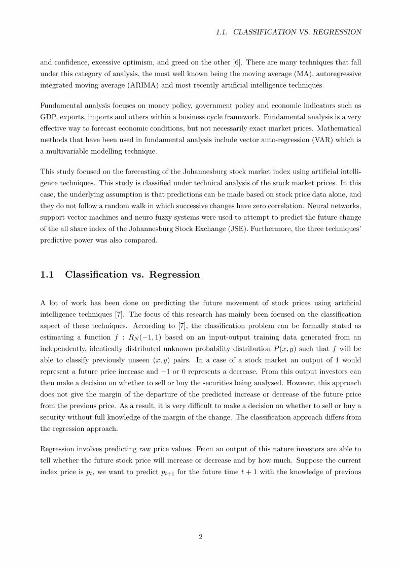
This study focused on the forecasting of the Johannesburg stock market index using artificial intelli-
gence techniques. This study is classified under technical analysis of the stock market prices. In this
case, the underlying assumption is that predictions can be made based on stock price data alone, and
they do not follow a random walk in which successive changes have zero correlation. Neural networks,
support vector machines and neuro-fuzzy systems were used to attempt to predict the future change
of the all share index of the Johannesburg Stock Exchange (JSE). Furthermore, the three techniques’
predictive power was also compared.
1.1 Classification vs. Regression
A lot of work has been done on predicting the future movement of stock prices using artificial
intelligence techniques [7]. The focus of this research has mainly been focused on the classification
aspect of these techniques. According to [7], the classification problem can be formally stated as
estimating a function f : RN (−1, 1) based on an input-output training data generated from an
independently, identically distributed unknown probability distribution P (x, y) such that f will be
able to classify previously unseen (x, y) pairs. In a case of a stock market an output of 1 would
represent a future price increase and −1 or 0 represents a decrease. From this output investors can
then make a decision on whether to sell or buy the securities being analysed. However, this approach
does not give the margin of the departure of the predicted increase or decrease of the future price
from the previous price. As a result, it is very difficult to make a decision on whether to sell or buy a
security without full knowledge of the margin of the change. The classification approach differs from
the regression approach.
Regression involves predicting raw price values. From an output of this nature investors are able to
tell whether the future stock price will increase or decrease and by how much. Suppose the current
index price is pt, we want to predict pt+1 for the future time t + 1 with the knowledge of previous
2
1.2. MOTIVATION
prices pt−n, pt−n+1, ....., pt−1, pt respectively. The prediction function is expressed as follows:
pt+1 = f(pt, pt−1, ......., pt−n) (1.1)
1.2 Motivation
The most fundamental motivation for trying to predict the stock market prices is financial gain. The
ability to uncover a mathematical model that can consistently predict the direction of the future
stock prices would make the owner of the model very wealthy. Thus, researchers, investors and
investment professionals are always attempting to find a stock market model that would yield them
higher returns than their counterparts.
1.3 Research Hypotheses
For this research, the following hypotheses have been identified and research outcomes will attempt
to test these hypotheses:
1. Neural networks can be used to forecast the future prices of the stock market
2. Neuro-fuzzy systems can be used to forecast the future prices of the stock market
3. Support Vector Machines can be used to forecast the future stock market prices of the stock
market
1.4 Objective of the Report
Many computational intelligence techniques have been applied to the problem of forecasting stock
prices. Most of the work that has been done in this area has neglected emerging markets especially
the South African market and has focused more on developed markets. Hence, the first objective of
this work is to apply neural networks, support vector machines and neuro-fuzzy to the forecasting
of the all share index of the Johannesburg Stock Exchange. The second objective is to compare
the accuracy of the prediction results of each tool. The three techniques are analysed on both their
strengths and their weaknesses.
3

1.5. STRUCTURE OF THE REPORT
It must be stated however, that it is not the objective of this report to develop a guideline for
investing on assets in the stock market. This work should be regarded as decision making support
tool when deciding to invest in the market.
1.5 Structure of the Report
A brief description of the structure of the thesis is given below:
Chapter 2 covers forecasting and the studies that have been done on forecasting.
Chapter 3 provides the background on the stock market and the different studies that have been
conducted on the Johannesburg Stock Exchange. This chapter describes the evolution of the
techniques used for stock market prediction. It also introduces the studies on application of
artificial intelligence techniques to financial time series.
Chapter 4 gives a description the three artificial intelligence techniques that are used for this re-
search namely, multilayer perceptron, support vector machines, and neuro-fuzzy system.
Chapter 5 covers the Autoregressive Moving Average modelling and forecasting.
Chapter 6 covers the application of multilayer perceptron, support vector machine, neuro-fuzzy
systems to the prediction of the All Share Index.
Chapter 7 summarises the findings and gives suggestions for future research.
4

Chapter 2
Forecasting
2.1 Introduction
Forecasting is an attempt to predict how a future event will occur. The main objective of forecasting
the occurrence of this event is for decision makers to make better decisions. There are two major
approaches to forecasting, namely explanatory (causal) and time series [8]. Explanatory forecasting
assumes a cause and effect relationship between the inputs and output. According to explanatory
forecasting, changing the inputs will affect the output of the system in a predictable way, assuming
the cause and effect relationship is constant. Unlike explanatory forecasting, time series forecasting
treats the system as a black box and endeavours to discover the factors affecting the behaviour.
There are two reasons for wanting to treat a system as a black box [8]. First, the system may not be
understood, and even if it were understood it may be extremely difficult to measure the relationships
assumed to govern its behaviour. Second, the main concern may be only to predict what will happen
and not why it happens. The financial time series is one of the least understood areas which has
been under scrutiny for some time for reasons that are well known (to improve investment returns).
Hence, the focus of this work is time series forecasting.
2.2 Criteria selection and comparison of forecasting methods
Various techniques have been developed over the years to conduct forecasting. The challenge has
always been to find a forecasting method that has the ability to give the best approximation of
the system that is being modelled. There are several ways in which the criteria for selecting and
comparing forecasting methods are organized. They could be organized in order of importance, and
accuracy is given the top priority. Other criteria used is the pattern of the data to be forecast, the
type of series, the time horizon to be covered in forecasting and the ease of application.
5
2.2. CRITERIA SELECTION AND COMPARISON OF FORECASTING METHODS
2.2.1 Accuracy
Accuracy is very important in determining whether to use a certain model to forecast future occur-
rences. The accuracy of a forecast can also reflect other factors, for example, insufficient data or use
of a technique that does not fit the pattern of the data which is reflected by less accurate forecasts [9].
It is desirable for a forecast to be accurate so that decision making becomes much easier in uncertain
situations. There are good reasons to support a forecast regardless of accuracy if the forecast is made
in a highly uncertain situation. Accuracy in this experiment is used to measure the deviation of the
forecasted results from the actual values. The issue that arises next is the approach that should be
taken in assessing the accuracy of the predictions from each of the methods used for forecasting.
Forecasters generally agree that forecasting methods should be assessed for accuracy using out-of-
sample tests rather than test for goodness of fit to past data (in-sample tests)[10]. Fildes and
Makridakis [11] concluded that the performance of a model on data sample outside that used in its
training or construction remains the touchstone for its utility in all applications. The out-of-sample
approach was adopted for this study to assess the forecasting accuracy of the constructed artificial
intelligence models.
2.2.2 Pattern of the data and its effects on individual forecasting methods
Patterns may represent characteristics that repeat themselves with time or they may represent turning
points that are periodic in nature. A data series can be described as consisting of two elements,
namely the underlying pattern and randomness. The objective of the forecast is to distinguish
between these two elements using the forecasting method that can appropriately do so. Time series
analysis has also revealed that a pattern itself can be thought of as consisting of sub-patterns or
components, namely trend, seasonality and cycle [8]. Understanding the three sub-patterns helps in
selecting the appropriate forecasting model, since different methods vary in their ability to cope with
different kinds of patterns.
2.2.3 Time horizon effects on forecasting methods
One of the reasons the time horizon is particularly important in selecting a forecasting method in a
given situation is that the relative importance of different sub-patterns changes as the time horizon of
planning changes. In the short term, randomness is usually the most important element. Then, in the
medium term the cyclical element becomes important and finally in the long term, the trend element
dominates. There is generally a greater uncertainty as the time horizon lengthens. Makridakis et
al [9] found that a major factor affecting the forecasting accuracy was the type of time series used.
6
2.3. ACCURACY MEASURE SELECTION
With micro data, exponential smoothing methods seemed to do much better than the statistically
sophisticated methodologies of ARMA, Bayesian forecasting, Parzen’s method and adaptive filtering.
Armstrong and Green [12] concluded as part of the general principles of forecasting that when
making forecasts in highly uncertain situations, be conservative. The financial time series is a highly
uncertain environment. Hence, this study is focused on a short-term forecasting horizon. The
artificial intelligence techniques were used to predict the next day’s price of the stock market index.
2.2.4 Ease of Application
Included under this heading are such things as complexity of the methods, the timeliness of the
forecasts it provides, the level of knowledge required for application, and the conceptual basics and
the ease with which it can be conveyed to the final user of the forecast [8]. One of the drawbacks
in adopting appropriate forecasting techniques is making the ultimate user comfortable with the
technique and its rationale so that the user can effectively judge the results of the forecasting method
and their usefulness. Artificial intelligence techniques are black boxes that are easy to use, however,
the user cannot work out how the results from these techniques were computed.
2.3 Accuracy measure selection
Conclusions about the accuracy of various forecasting methods typically require comparisons across
many time series. However, it is often difficult to obtain a large number of series. This is particularly
a problem when trying to specify the best method for a well-defined set of conditions; the more
specific the conditions, the greater the difficulty in obtaining many series. Thus, it is important
to identify which error measures are useful given few series, and which are appropriate for a larger
number of series. Error measures also play an important role in calibrating or refining a model so
that it can forecast accurately for a set of time series. That is, given a set of time series, the analyst
may wish to examine the effects of using different parameters in an effort to improve a model.
For selection among forecasting methods, the primary criteria are reliability, construct validity, pro-
tection against outliers, and the relationship to decision making [13]. Sensitivity is not so important
for selecting methods. Given a moderate number of series, reliability becomes a less important
issue. The Mean Absolute Percentage Error (MAPE) would be appropriate because of its closer
relationship to decision making [13], is reliable and protects against outliers. Various accuracy mea-
surement methods were considered for this experiment to compare the differences in their accuracy
measurement. For further details refer to Appendix C.
7
2.4. IN-SAMPLE VERSUS OUT-OF-SAMPLE EVALUATION
2.4 In-sample versus out-of-sample evaluation
Researchers have generally reached a consensus that forecasting methods should be assessed for
accuracy using out-of-sample tests as opposed to goodness of fit to past data or in-sample tests. ‘The
performance of a model on data outside that used in its construction remains the touchstone for its
utility in all applications’ [11]. Two reasons have been advanced by practitioners of the forecasting
research for this conclusion to be reached. The first reason is that for a given forecasting model, in-
sample errors are likely to understate forecasting errors. Model selection and estimation are designed
to calibrate a forecasting procedure of historical data. Past data and future data are likely to have
different dynamics and this may have an effect on model selected.
Overfitting and structural changes may occur, which may further aggravate the inconsistent perfor-
mance between in-sample and post-sample data. The M-competition study by Makridakis et al. [15]
and many subsequent empirical studies show that forecasting errors generally exceed in-sample er-
rors, even at reasonably short horizons. In addition, prediction intervals built on in-sample standard
errors are likely to be too narrow [16].
The second reason is that, a model that is selected on the basis of best in-sample fit may not be
best to predict out-of-sample data. Research conducted by Bartolomei and Sweet [17] and Pant and
Starbuck [18] reaches this conclusion convincingly. As already stated an out-of-sample evaluation
approach was adopted for this work.
2.5 Transaction costs and forecasting
Transaction costs and trading restrictions change tests of market efficiency in some important ways.
Most obviously, if transaction costs are very high, predictability is no longer ruled out by arbitrage,
since it would be too expensive to take advantage of even a large, predictable component in returns
[19]. An investor may predict that a particular stock is going to outperform the market by 4 percent
the following day, but if the transaction cost from buying the asset is 6 percent, then it may not
be profitable to exploit this prediction. Predictability therefore has to be seen in relation to the
transaction costs of the asset. Predictable patterns only invalidate the EMH once they are large
enough to cover the size of transaction costs.
The existence of a single successful prediction model is not sufficient to demonstrate violation of the
efficient market hypothesis (EMH), which is covered in chapter 3 in greater detail, the model has to
give predictions that allow the investor to cover transaction cost and still make a profit.
Transactions costs of trading shares in the Johannesburg Stock Exchange are as follows [20]:
8
2.6. FORECASTING STUDIES
1. Brokerage fee paid for every transaction
2. Securities Transfer Tax (STT) for purchases of shares only
3. A STRATE charged fee
4. A financial services board (FSB) levied investor protection levy which applies to all trades
Return from a daily share trade is defined by the following equation [21]:
Return =Pt+1 − Pt +Dt
Pt(2.1)
where Pt+1 is the next day’s price, Pt is today’s price and Dt is the dividend. Equation 2.1 (the one
step ahead prediction return) depends on:
1. The magnitude of the price increase
2. The accuracy of the prediction
3. Number of shares (volume) to be traded
2.6 Forecasting studies
In 1969 Reid [22] and Newbold and Granger[23] compared a large number of series to determine
their post-sample forecasting accuracy. However, the first effort to compare a large number of major
time series methods was conducted by Makridakis and Hibon [9]. Their major conclusion was that
sophisticated statistical methods do not necessarily outperform simple methods such as exponen-
tial smoothing. The conclusion was heavily criticised, because it went against conventional wisdom.
Makridakis, continued with the studies by launching M-competition (forecasting competition orga-
nized by Spyros Makridakis where forecast errors of forecasting methods were compared for forecasts
of a variety of economic time series) to respond to criticisms. This study included a variety of time
series, 1001 time series, and 15 forecasting methods. Various accuracy measures were used.
The results of the M-competition were not different from the earlier conclusions made by Makridakis
and Hibon [9]. The study summarised its findings as follows:
1. Statistically sophisticated or complex methods do not necessarily provide more accurate fore-
casts than simpler ones.
9

2.6. FORECASTING STUDIES
2. The relative ranking of the performance of the various methods varies according to the accuracy
measure being used.
3. The accuracy when various methods are combined, outperforms, on average, the individual
methods being combined.
4. The accuracy of the various methods depends upon the length of the forecasting horizon in-
volved.
Using the same data that was used for M-competition, Hill et al [24], Koeler et al [25], and Lusk et al
[26], reached similar conclusions. Finally, additional studies Armstrong and Callopy [13] and Makri-
dakis [15], Fildes et al [27] using other data series reached the above four conclusions. Makridakis
went on to launch M2 and M3 competitions and they reinforced the same conclusions. However,
artificial intelligence techniques were not included in the first and second M-competitions. M3 in-
cluded radial basis function (RBF) and automated artificial neural networks (Auto ANN). Therefore,
further studies that would include most of the artificial intelligence techniques are required to study
whether the conclusions mentioned above still hold true.
10

Chapter 3
The market
3.1 Johannesburg Stock Exchange
The Johannesburg Stock Exchange (JSE) describes itself as follows [20]:
“More than a forum for trading shares and bonds, the JSE stands tall as the engine-room of the
South African economy. Here, companies from the spectrum of industry and commerce gather to
raise the public capital that will allow them to expand, in the process creating new jobs, products,
services and opportunities.”
The JSE was established on 8 November 1887 and was housed on stands at the corner of Commissioner
and Simmonds Streets, Johannesburg. In 1903 the JSE moved to new premises in Hollard Street
which became the financial centre of Johannesburg and was to remain so for more than half a century.
In February 1960 the fourth exchange in Hollard Street was built on the same site as the old exchange.
During construction a temporary home was found for the JSE in Protection House in Fox Street.
On 12 December 1978 (fifth move) the JSE took up residence at 17 Diagonal Street where JSEs
stockbrokers, staff and offices were all housed in two buildings next door to each other. In September
2000, the JSE moved premises for the sixth time to One Exchange Square, corner Maude Street and
Gwen Lane in Sandton [20].
3.1.1 What is Market index?
A market index is defined as a statistical measure of the changes in a portfolio of shares representing a
portion of the overall market [20]. The fluctuations of the market are represented by the index of that
market. Essentially the index of the market is a smaller sample of the market that is representative
of the whole. With the growing importance of the shares market in different societies, indices like
11

3.2. EFFICIENT MARKET HYPOTHESIS
the JSE All Share, the FTSE, DJIA, Nikkei and Nasdaq composite have grown to become part of
everyday vocabulary. The index is used as a measure of the performance of the market and the
change in the price of the index represents the proportional change of the shares included in the
index.
The JSE has different indices with different portfolios of shares which includes the following:
1. All Share Index. This is the main index in the Johannesburg stock exchange. It consists of
62 stocks in total. It is made up of the top 40 shares by market capitalisation and 22 shares
from across all sectors and industries.
2. Alsi 40 Index. It is made up of the top 40 companies by market capitalisation.
3. All Gold Index. It is a weighted average of all the companies that mine gold that are listed
on the JSE.
3.2 Efficient Market Hypothesis
The testing of the EMH has been investigated by many researchers. The term “efficient market” was
first introduced by E.F. Fama [2] in a paper of 1965 where he stated that for efficient markets on
average, competition will cause the full effects of new information on intrinsic values to be reflected
“instantaneously” in actual prices. It was believed that when information arises, the news spread
very quickly and is incorporated into the prices of securities without delay. The implication of this
hypothesis is that technical analysis of securities and fundamental analysis of the companies would
not yield any more extraordinary returns for the investors than a “buy or hold” strategy.
EMH is related to the concept of “random walk” which asserts that future stock prices randomly
depart from the past prices [2]. The reason for the “random walk” is that new information is
immediately reflected on the stock price and the future price will also reflect information which
comes randomly. The absence of the predictability of the prices makes the “buy or hold” strategy
the most appropriate. There are three types of EMH:
Weak-Form Efficiency - this form of efficiency states that the past price information is fully
incorporated in the current price and does not have any predictive power. This means that
predicting the future returns of an asset based on technical analysis is impossible.
Semi-Strong Form Efficiency - this form of efficiency states that any public information is fully
incorporated in the current price of an asset. Public information includes the past prices and
12

3.2. EFFICIENT MARKET HYPOTHESIS
also the data reported in a company’s financial statements, earnings and dividends announce-
ments, the financial situation of company’s competitor, expectations regarding macroeconomic
factors, etc.
Strong Form Efficiency - this form of efficiency states that the current price incorporates all in-
formation, both public and private. This means that no market actor can be able to consistently
derive profits even if trading with information that is not already public knowledge.
EMH is a statement about: (1) the assertion that stock prices reflect the true value of stocks; (2) the
absence of arbitrage opportunities in the economy dominated by rational, profit maximizing agents;
(3) the hypothesis that all available information comes to the market randomly and is fully reflected
on the market prices [4]. Fama [4] presented a general notation describing how investors generate
price expectations for stocks. This could be explained by Cuthbertson as [28]:
E (pj,t+1|φt) = [1 + E (rj,t+1|φt)] pjt (3.1)
where E is the expected value operator, pj,t+1 is the price of security j at time t + 1, rj,t+1 is the
return on security j during period t + 1, and φt is the set of information available to investors at
time t. The left-hand side of the formula E (pj,t+1 |φt) denotes the expected end-of-period price on
stock j, given the information available at the beginning of the period φt. On the right-hand side,
1 +E (rj,t+1 |φt) denotes the expected return over the forthcoming time period of stocks having the
same amount of risk as stock j.
Under the efficient market hypothesis, market agents cannot earn excessive profits on the available
information set other than by chance. The level of over value or under value of a particular stock is
defined as [28]:
xj,t+1 = pj,t+1 − E (pj,t+1|φt) (3.2)
where xj,t+1 indicates the extent to which the actual price for security j at the end of the period
differs from the price expected by investors based on the information available φt. As a result, in an
efficient market it must be true that [28]:
E (xj,t+1|φt) = 0 (3.3)
This implies that the information is fully incorporated in stock prices. Therefore the rational ex-
pectations of the returns for a particular stock according to the EMH may be represented as [28]:
Pt+1 = EtPt+1 + εt+1 (3.4)
where Pt is the stock price; and εt+1 is the forecast error. Pt+1 −EtPt+1 should therefore be zero on
average and should be uncorrelated with any information φt. Also E (xj,t+1 |φt) = 0 when random
13
3.2. EFFICIENT MARKET HYPOTHESIS
variable (good or bad news) and the expected value of the forecast error, is zero:
Etεt+1 = Et (Pt+1 − EtPt+1) = EtPt+1 − EtPt+1 = 0 (3.5)
Underlying the efficiency market hypothesis, it is opportune to mention that expected stock returns
are entirely consistent with randomness in security returns.
3.2.1 Studies evaluating EMH
Previous empirical studies of testing EMH have mainly used econometric models such as the run test,
serial correlation test and the variance ratio test. The serial correlation test and the run tests are
used to test the dependence of share prices. Finding some form of dependency in stock prices allows
forecasters to use these relationships to predict future prices or returns, thus, refuting EMH [29].
This kind of test focuses on the weak-form of efficiency. The validity of the hypothesis is confirmed
by finding zero correlation. Fama [2] did a study on a sample of 30 Dow Jones industrial stocks and
found that the serial correlation which existed was too small to cover the transaction costs of trading.
Brock et al [30] found that the simple technical trading rules would have been able to predict the
changes in the Dow Jones industrial average. Subsequent research has found that the gains from
the strategies are not enough to cover the transaction costs. Indeed, these studies are consistent
with the weak-form efficiency. Another way of testing this kind of efficiency is to find statistical
relationships between past prices and future prices. These statistical relationships allow forecasters
to make predictions about future stock market returns. Various statistical methods have been used
to test the EMH such as Auto Regressive Conditional Heteroskedasticity (ARCH), Generalised Auto
Regressive Conditional Heteroskedasticity (GARCH) and Auto Regressive Moving Average (ARMA)
[6][31][32]. One can argue that the traditional econometric approach based on models with simple
specifications and constant parameters, such as Box-Jenkins ARMA models, are unable to respond
to the dynamics inherent in economic and financial series [19]. However, the debate concerning the
gains coming from the use of nonlinear models has not reached a consensus yet [33], stimulating
further research in areas such as nonlinear model selection, estimation and evaluation approaches.
Semi-strong efficiency is concerned with publicly available information. The test for this form of
efficiency focuses on the evaluation of the speed and accuracy of the adjustment of the stock prices
due to the availability of the information. The information that creates significant adjustments in
the stock prices includes price earning announcements, changes of dividend policy, capitalizations,
announcements of merger plans, the financial situation of the competition, expectations regarding
macroeconomic factors etc. To test this form of efficiency is rather complex. The way it is usually
done is to try and predict a future price using different asset pricing methodologies and then compare
the price to the adjusted one. The difference of the two prices is then analyzed to determine the
speed and the accuracy of the adjustments [29].
14
3.3. MODELLING STOCK PRICES OR RETURN
The strong-form of efficiency is tested by evaluating whether there are individuals who have access
to private information that helps them to earn above average return in the market. If there is an
investor who persistently outperforms the market then there is evidence for the lack of strong form
efficiency [29].
3.3 Modelling stock prices or return
Short term forecasting problems are concerned with prediction of variation under the assumption
that the essential nature of the process will continue. It is appropriate to try to determine fixed rules
to predict the near future from the recent past. As a result a variety of fixed mathematical models
have been developed for this task. These models have ranged from smoothing models to complex
econometric models. The fulcrum of the different mathematical forecasting models has always been
to attain the maximum accuracy. This means finding the best forecasting model that can represent
the problem based on the given information. The availability of extensive historical information
makes it possible to derive a statistical forecaster based on this data, which can predict better than
the ones chosen by judgment. Various forecasting models have been developed to predict the future
based on past observations.
3.3.1 Previous techniques
Forecasting models have evolved over the years and the complexity of these models has also increased
to be able to deal with increasing complexity of the markets. This section presents the different models
that have been used previously and the ones that are being used currently and the ones that are still
under research.
(a) Smoothing
Smoothing methods are used to determine the average value around which the data is fluctuating.
Two examples of this type of approach are the moving average and exponential smoothing. Mov-
ing averages are constructed by summing up a series of data and dividing by the total number of
observations. The total number of observations is determined arbitrarily to compromise between
stability and the responsiveness of the forecaster. Moving average is probably the most widely used
method of identifying trends, since they do a good job of smoothing out these random fluctuations
[34]. Exponential smoothing is constructed in such a way that the forecast value is a weighted aver-
age of the preceding observations, where the weights decrease with the age of the past observations.
Exponential smoothing has one or more parameters which determine the rate of decrease of the
15
3.3. MODELLING STOCK PRICES OR RETURN
weights. These parameters can be determined arbitrarily or by other intuitive methods such as the
least squares method.
(b) Curve fitting
A graph of the history of different time series processes sometimes exhibits characteristic patterns
which repeat themselves over time. The tendency to extrapolate such is often hard to resist. A
number of forecasting methods have been based on the premise that such extrapolation is a reason-
able thing to do. Curve fitting, or data mining, is the ‘art’ of drawing conclusions based on past
information. When applied to an investment scheme or trading strategy, history shows that often
such conclusions do not hold true once they are implemented [36].
3.3.2 Techniques based on mathematics
(a) Linear modelling
Linear regression forecasting models have demonstrated their usefulness in predicting returns in both
developed markets and developing markets [37]. Linear regression models that have been tested can
correctly predict direction in the market over 55-65 percent of the time. It was established that
random walk hypothesis, which assumes that the best prediction for the future price is the current
price, could predict the direction of market prices 50 percent of the time [37]. It may be reasonable to
state at this point that nonlinearities in the behaviour of the stock market prices could be the cause
of this inability of linear methods to exhibit significant superiority over random walk hypothesis.
For this reason, linear regression methods have been unable to give satisfactory results for investors.
Autoregressive-integrated moving average (ARIMA) [34] which is a univariable model, is one the
linear techniques that has been extensively used to try to predict the direction of market prices.
The ARIMA model is able to transform non-stationary time series to stationary time series using
a process called differencing. In [38] higher order statistical techniques were found to be superior
to ARIMA models. Linear models are simple and as a result tend to want to simplify a system
as complicated as financial market behaviour. However, the advantage of linear models lies in the
simplicity. A model is only useful as long as its predictions do not deviate too far from the outcome
of the underlying process. With linear models there is a trade off between simplicity and accuracy
of the predictions.
16
3.3. MODELLING STOCK PRICES OR RETURN
(b) Non-linear modelling
It is conventional thinking that linear forecasting models are very poor in terms of capturing the un-
derlying dynamics of the financial time series. In recent years, the discovery of non-linear movements
in the financial markets has been greatly emphasised by various researchers and financial analysts
[39]. Chan and Tong [40] argues strongly that for non-linear models ‘how well we can predict depends
on where we are’ and that there are ‘windows of opportunity for substantial reduction in prediction
errors’. A large amount of research has documented evidence of nonlinearities in stock returns. One
element of this has been the mounting evidence that the conditional distribution of stock returns is
well represented by a mixture of normal distributions (e.g. see Ryden, Terasvirta et al [41] and the
references therein) and that, as result , a Markov switching model may be a logical characterization of
stock returns behaviour (e.g. see, inter alia, LeBaron,[42]; Hamilton and Susmel, [43]; Hamilton et al,
[38]; Ramchand et al, [44, 45]; Ryden et al, [41]; Susmel, [46]). The relevant literature suggests that
not only Markov switching models fit stock returns data well, but they may perform satisfactorily in
forecasting (e.g. see Hamilton et al, [43]; Hamilton et al, [38]).
Non-linear models are much more complicated than linear models and therefore much more difficult
to construct. Part of the reason for this difficulty is the number of diverse models which is higher for
non-linear models making it difficult for one to choose a suitable model. Research has established
some methods of identifying non-linear models such as non-linear regression, parametric models such
GARCH, and non-linear volatility models and nonparametric models.
The debate concerning the gains coming from the use of nonlinear models has not reached a con-
sensus yet [33], stimulating further research in areas such as nonlinear model selection, estimation
and evaluation approaches. Artificial intelligence techniques such as neural networks and support
vector machines are also under investigation to further the research of non-linear models. Even
though there are a number of non-linear statistical techniques that have been used to produce better
predictions of future stock returns or prices, most techniques are model-driven approaches which
require that the non-linear model be specified before the estimation of parameters can be deter-
mined. In contrast, artificial intelligence techniques are data-driven approaches which do not require
a pre-specification during the modelling process because they independently learn the relationship
inherent in the variables. Thus, neural networks are capable of performing non-linear modelling
without a priori knowledge about the relationship between input and output variables. As a result,
there has been a growing interest in applying artificial intelligence techniques to capture future stock
behaviours; see [47, 48, 49, 50], for previous work on stock predictions.
Among the different nonlinear methods artificial neural networks are being used by forecasters as a
non-parametric regression method [51]. The advantage with using neural networks (NN) is that as
a non-linear approximator it exhibits superiority when compared to other non-linear models. The
reason is because NN is able to establish relationships in areas where mathematical knowledge of the
17
3.4. SOUTH AFRICAN STUDIES
stochastic process underlying the analyzed time series is unknown and difficult to rationalise [52]. In
another case, a back propagation neural network developed by Tsibouris and Zeidenburg [53], that
only used past share prices as input had some predictive ability, which refuted the weak form of the
EMH. In contrast, a study on IBM stock movement by [54], did not find evidence against the EMH.
Mukherjee et al. [55], showed the applicability of support vector machines (SVM) to time-series
forecasting. Recently, Tay and Cao [56], examined the predictability of financial time-series including
five time series data with SVMs. They showed that SVMs outperformed the Back Propagation
networks on the criteria of normalised mean square error, mean absolute error, directional symmetry
and weighted directional symmetry. They estimated the future value using the theory of SVM in
regression approximation. Some applications of SVM to financial forecasting have been reported
recently [55]. SVM as shown by [57] is superior to the other individual classification methods in
forecasting the weekly movement direction of NIKKEI 225 Index.
Practical applications of fuzzy systems include systems for stock selection [58], foreign exchange
trading [50], etc. Chen et al [59] used fuzzy time-series to forecast the Taiwan stock market. Fuzzy
logic is also used to improve the effectiveness of neural networks by “incorporating structured knowl-
edge about financial markets, including rules provided by traders, and explaining how the output or
trading recommendations were derived” [69].
3.4 South African studies
The JSE attracts investors from all over the world who scramble to gain access to mineral resources
companies that are traded in the market. As a result the JSE has attracted different types of studies
attempting to model the behaviour of stocks. South Africa as an emerging market provides an
interesting case to study because of the different perceptions that investors have about emerging
markets in general. Prediction of the emerging markets is very difficult due to the volatility of
the returns [74]. Emerging markets are believed to be less informationally efficient than developed
markets and this inefficiency can be exploited in a forecasting model.
A study done by [75] focused on testing if there are anomalies on the JSE, namely the day-of-the-
week effect, the week-of-the-month effect, the month-of-year effect, the turn-of-the-month effect, the
turn-of-the-year effect and a quarterly effect using Anova, an F-test and the Krustal Wallis test. This
study was concluded by finding evidence of week-of-the-month effect and turn-of-the-month effect.
Studies on whether the JSE is efficient have also been conducted. A study was conducted on 11
South African unit trusts for the period 1970-1976 by [76] and he found evidence for a strong form of
efficiency. The study was later contradicted by [77], who found there was no evidence for the strong
form of efficiency on their analysis of 11 unit trusts for the period of between 1977-1986. Weak
18

3.4. SOUTH AFRICAN STUDIES
form of efficiency was tested and rejected by Jammine and Hawkins [78] based on the study they
did on JSE shares for the period 1966-1973. Jammine and Hawkins study was later contradicted by
Affleck-Graves and Money [79] who tested the EMH at the JSE and found evidence for the weak
form of efficiency. The debate has never been concluded as to whether the JSE is efficient or not.
Several studies have also been conducted on modelling the market. Van Rensburg made the largest
contribution to the study of the stock market and modelling. In his study, Van Rensburg [80] found
that four economic factors, namely the unexpected change in the term structure, unexpected returns
of the New York stock exchange, unexpected changes in inflation expectations and expected changes
in the gold price significantly influences JSE stock prices. Van Rensburg [81] studied the correlations
between stock market returns and macroeconomic variables. In 1999 Van Rensburg [82] concluded
that long run interest rate, the gold and the foreign reserve balance and the balance on the current
account significantly influences the returns of the JSE overall index, the industrial index and the gold
index.
Several studies have been conducted on the South African market to evaluate the behaviour of the
prices. Some of these studies were focused on testing efficiency and existence of anomalies on the
(JSE). A very extensive system [49], which modeled the performance of the Johannesburg stock
Exchange and based its trading decisions on 63 indicators demonstrated superior performance and
was able to predict stock market directions thus refuting EMH. Patel and Marwala [48] used neural
networks to predict the Allshare index in the JSE using past index prices and they found that it was
predictable. Another study used neural networks, fuzzy inference systems and adaptive-neurofuzzy
inference systems for financial decision making in the Johannesburg Stock Exchange [47].
The review of the literature indicates that studies with contradictory conclusions have been conducted
over the years on the South African market. Most of the studies have been conducted using old
regression techniques and artificial intelligence techniques have been introduced recently. A further
study is required on the predictability of the JSE and this study is aimed at contributing to the
literature and also to attempt to settle the EMH debate. This study will focus on introducing
other artificial intelligence tools to try and forecast the future price of the stock market index of the
Johannesburg Stock Exchange.
19

Chapter 4
Artificial intelligence techniques
The chapter aims to introduce the reader to the three artificial intelligence (AI) techniques that
were used for this work. AI is the science and engineering of making intelligent machines, especially
intelligent computer programs. It is related to the similar task of using computers to understand
human intelligence, but AI does not have to confine itself to methods that are biologically observable.
Intelligence is the computational part of the ability to achieve goals in the world. In this work
multilayer perceptron neural networks, support vector machines and neuro-fuzzy systems are used
for the prediction of the stock market index.
4.1 Neural networks
The theory of neural network (NN) computation provides interesting techniques that mimic the
human brain and nervous system. A neural network is characterized by the pattern of connections
among the various network layers, the numbers of neurons in each layer, the learning algorithm,
and the neuron activation functions. In general, a neural network is a set of connected input and
output units where each connection has a weight associated with it. Neural networks can be used
for classification or regression. For this study neural networks were used as a regression tool for
predicting the future price of a stock market index.
Neural networks gained interest after McCulloch and Pitts introduced a simple version of a neuron
in 1943 [83]. This model of a neuron was inspired by the biological neuron in the human brain and
it was presented as a simple mathematical model. Neural network is a network consisting of neurons
and paths connecting the neurons. Figure 4.1 shows a model of a neuron and how it connects into a
network. They are interconnected assemblies of simple processing nodes whose functionality is loosely
based on the animal neuron. NN can also be defined as generalisations of classical pattern-oriented
techniques in statistics and engineering areas of signal processing, system identification and control.
20
4.1. NEURAL NETWORKS
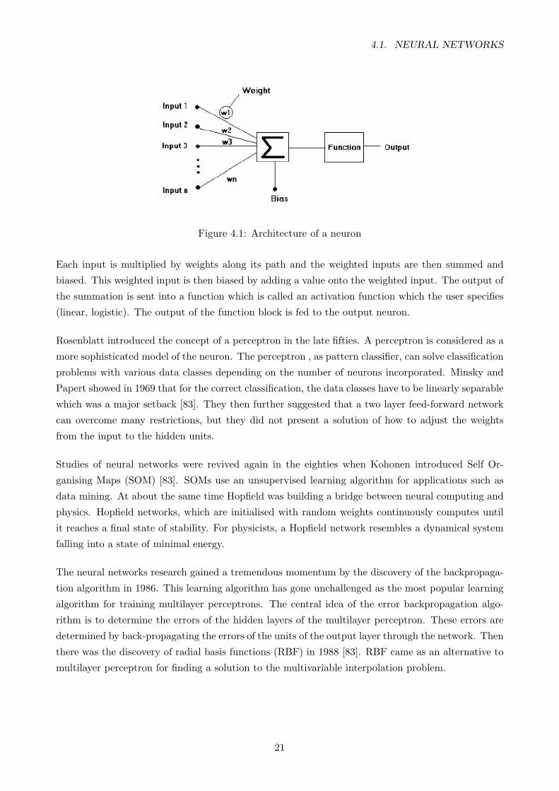
Figure 4.1: Architecture of a neuron
Each input is multiplied by weights along its path and the weighted inputs are then summed and
biased. This weighted input is then biased by adding a value onto the weighted input. The output of
the summation is sent into a function which is called an activation function which the user specifies
(linear, logistic). The output of the function block is fed to the output neuron.
Rosenblatt introduced the concept of a perceptron in the late fifties. A perceptron is considered as a
more sophisticated model of the neuron. The perceptron , as pattern classifier, can solve classification
problems with various data classes depending on the number of neurons incorporated. Minsky and
Papert showed in 1969 that for the correct classification, the data classes have to be linearly separable
which was a major setback [83]. They then further suggested that a two layer feed-forward network
can overcome many restrictions, but they did not present a solution of how to adjust the weights
from the input to the hidden units.
Studies of neural networks were revived again in the eighties when Kohonen introduced Self Or-
ganising Maps (SOM) [83]. SOMs use an unsupervised learning algorithm for applications such as
data mining. At about the same time Hopfield was building a bridge between neural computing and
physics. Hopfield networks, which are initialised with random weights continuously computes until
it reaches a final state of stability. For physicists, a Hopfield network resembles a dynamical system
falling into a state of minimal energy.
The neural networks research gained a tremendous momentum by the discovery of the backpropaga-
tion algorithm in 1986. This learning algorithm has gone unchallenged as the most popular learning
algorithm for training multilayer perceptrons. The central idea of the error backpropagation algo-
rithm is to determine the errors of the hidden layers of the multilayer perceptron. These errors are
determined by back-propagating the errors of the units of the output layer through the network. Then
there was the discovery of radial basis functions (RBF) in 1988 [83]. RBF came as an alternative to
multilayer perceptron for finding a solution to the multivariable interpolation problem.
21
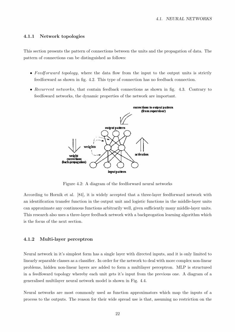
4.1. NEURAL NETWORKS
4.1.1 Network topologies
This section presents the pattern of connections between the units and the propagation of data. The
pattern of connections can be distinguished as follows:
• Feedforward topology, where the data flow from the input to the output units is strictly
feedforward as shown in fig. 4.2. This type of connection has no feedback connection.
• Recurrent networks, that contain feedback connections as shown in fig. 4.3. Contrary to
feedfoward networks, the dynamic properties of the network are important.
Figure 4.2: A diagram of the feedforward neural networks
According to Hornik et al. [84], it is widely accepted that a three-layer feedforward network with
an identification transfer function in the output unit and logistic functions in the middle-layer units
can approximate any continuous functions arbitrarily well, given sufficiently many middle-layer units.
This research also uses a three-layer feedback network with a backprogation learning algorithm which
is the focus of the next section.
4.1.2 Multi-layer perceptron
Neural network in it’s simplest form has a single layer with directed inputs, and it is only limited to
linearly separable classes as a classifier. In order for the network to deal with more complex non-linear
problems, hidden non-linear layers are added to form a multilayer perceptron. MLP is structured
in a feedfoward topology whereby each unit gets it’s input from the previous one. A diagram of a
generalised multilayer neural network model is shown in Fig. 4.4.
Neural networks are most commonly used as function approximators which map the inputs of a
process to the outputs. The reason for their wide spread use is that, assuming no restriction on the
22
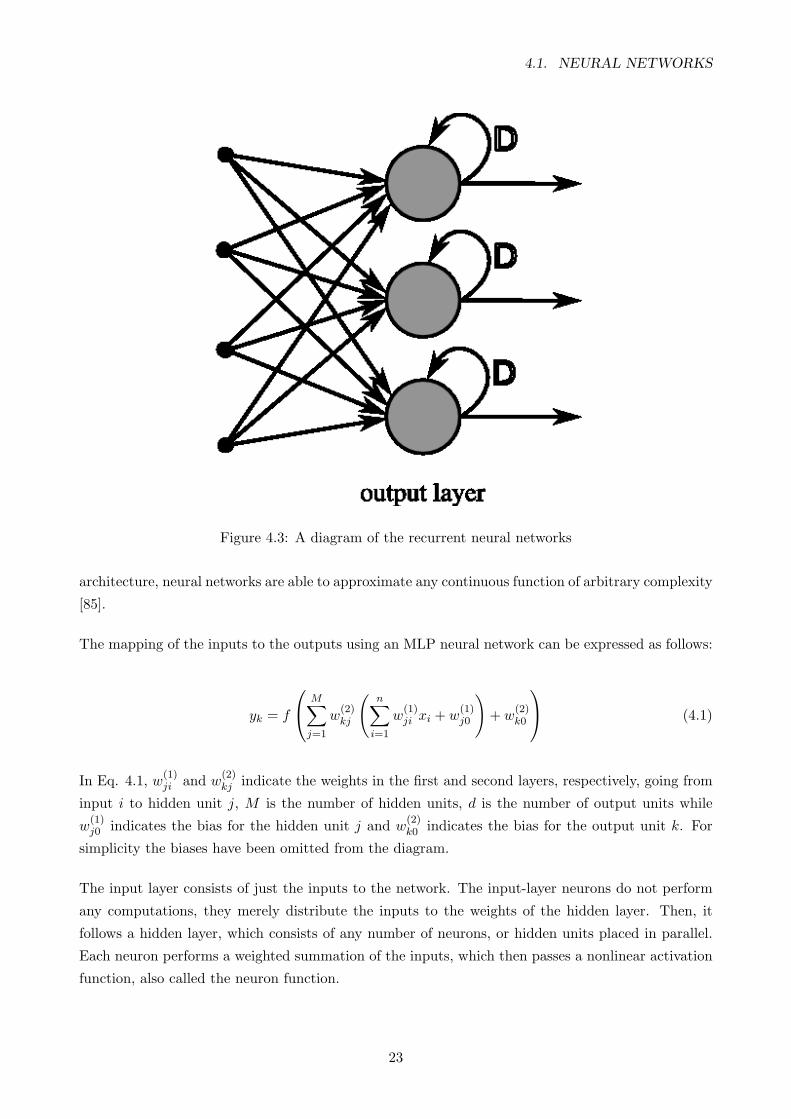
4.1. NEURAL NETWORKS
Figure 4.3: A diagram of the recurrent neural networks
architecture, neural networks are able to approximate any continuous function of arbitrary complexity
[85].
The mapping of the inputs to the outputs using an MLP neural network can be expressed as follows:
yk = f
M∑j=1
w(2)kj
(n∑
i=1
w(1)ji xi + w
(1)j0
)+ w
(2)k0
(4.1)
In Eq. 4.1, w(1)ji and w(2)
kj indicate the weights in the first and second layers, respectively, going from
input i to hidden unit j, M is the number of hidden units, d is the number of output units while
w(1)j0 indicates the bias for the hidden unit j and w
(2)k0 indicates the bias for the output unit k. For
simplicity the biases have been omitted from the diagram.
The input layer consists of just the inputs to the network. The input-layer neurons do not perform
any computations, they merely distribute the inputs to the weights of the hidden layer. Then, it
follows a hidden layer, which consists of any number of neurons, or hidden units placed in parallel.
Each neuron performs a weighted summation of the inputs, which then passes a nonlinear activation
function, also called the neuron function.
23
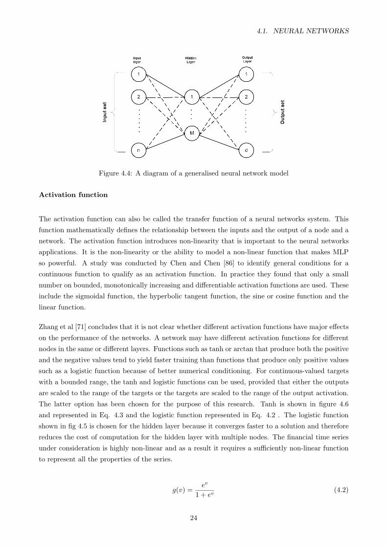
4.1. NEURAL NETWORKS
Figure 4.4: A diagram of a generalised neural network model
Activation function
The activation function can also be called the transfer function of a neural networks system. This
function mathematically defines the relationship between the inputs and the output of a node and a
network. The activation function introduces non-linearity that is important to the neural networks
applications. It is the non-linearity or the ability to model a non-linear function that makes MLP
so powerful. A study was conducted by Chen and Chen [86] to identify general conditions for a
continuous function to qualify as an activation function. In practice they found that only a small
number on bounded, monotonically increasing and differentiable activation functions are used. These
include the sigmoidal function, the hyperbolic tangent function, the sine or cosine function and the
linear function.
Zhang et al [71] concludes that it is not clear whether different activation functions have major effects
on the performance of the networks. A network may have different activation functions for different
nodes in the same or different layers. Functions such as tanh or arctan that produce both the positive
and the negative values tend to yield faster training than functions that produce only positive values
such as a logistic function because of better numerical conditioning. For continuous-valued targets
with a bounded range, the tanh and logistic functions can be used, provided that either the outputs
are scaled to the range of the targets or the targets are scaled to the range of the output activation.
The latter option has been chosen for the purpose of this research. Tanh is shown in figure 4.6
and represented in Eq. 4.3 and the logistic function represented in Eq. 4.2 . The logistic function
shown in fig 4.5 is chosen for the hidden layer because it converges faster to a solution and therefore
reduces the cost of computation for the hidden layer with multiple nodes. The financial time series
under consideration is highly non-linear and as a result it requires a sufficiently non-linear function
to represent all the properties of the series.
g(v) =ev
1 + ev(4.2)
24
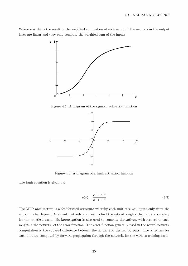
4.1. NEURAL NETWORKS
Where v is the is the result of the weighted summation of each neuron. The neurons in the output
layer are linear and they only compute the weighted sum of the inputs.
Figure 4.5: A diagram of the sigmoid activation function
Figure 4.6: A diagram of a tanh activation function
The tanh equation is given by:
g(v) =ev − e−v
ev + e−v(4.3)
The MLP architecture is a feedforward structure whereby each unit receives inputs only from the
units in other layers . Gradient methods are used to find the sets of weights that work accurately
for the practical cases. Backpropagation is also used to compute derivatives, with respect to each
weight in the network, of the error function. The error function generally used in the neural network
computation is the squared difference between the actual and desired outputs. The activities for
each unit are computed by forward propagation through the network, for the various training cases.
25
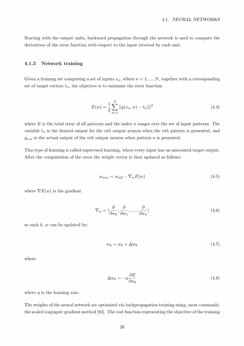
4.1. NEURAL NETWORKS
Starting with the output units, backward propagation through the network is used to compute the
derivatives of the error function with respect to the input received by each unit.
4.1.3 Network training
Given a training set comprising a set of inputs xn, where n = 1, .....N , together with a corresponding
set of target vectors tn, the objective is to minimise the error function.
E(w) =12
N∑n=1
||y(xn, w)− tn)||2 (4.4)
where E is the total error of all patterns and the index n ranges over the set of input patterns. The
variable tn is the desired output for the nth output neuron when the nth pattern is presented, and
yn,w is the actual output of the nth output neuron when pattern n is presented.
This type of learning is called supervised learning, where every input has an associated target output.
After the computation of the error the weight vector is then updated as follows:
wnew = wold −∇wE(w) (4.5)
where ∇E(w) is the gradient.
∇w = [∂
∂w0,∂
∂w1, .....,
∂
∂wn] (4.6)
so each k, w can be updated by:
wk = wk + ∆wk (4.7)
where
∆wk = −η ∂E∂wk
(4.8)
where η is the learning rate.
The weights of the neural network are optimised via backpropagation training using, most commonly,
the scaled conjugate gradient method [83]. The cost function representing the objective of the training
26
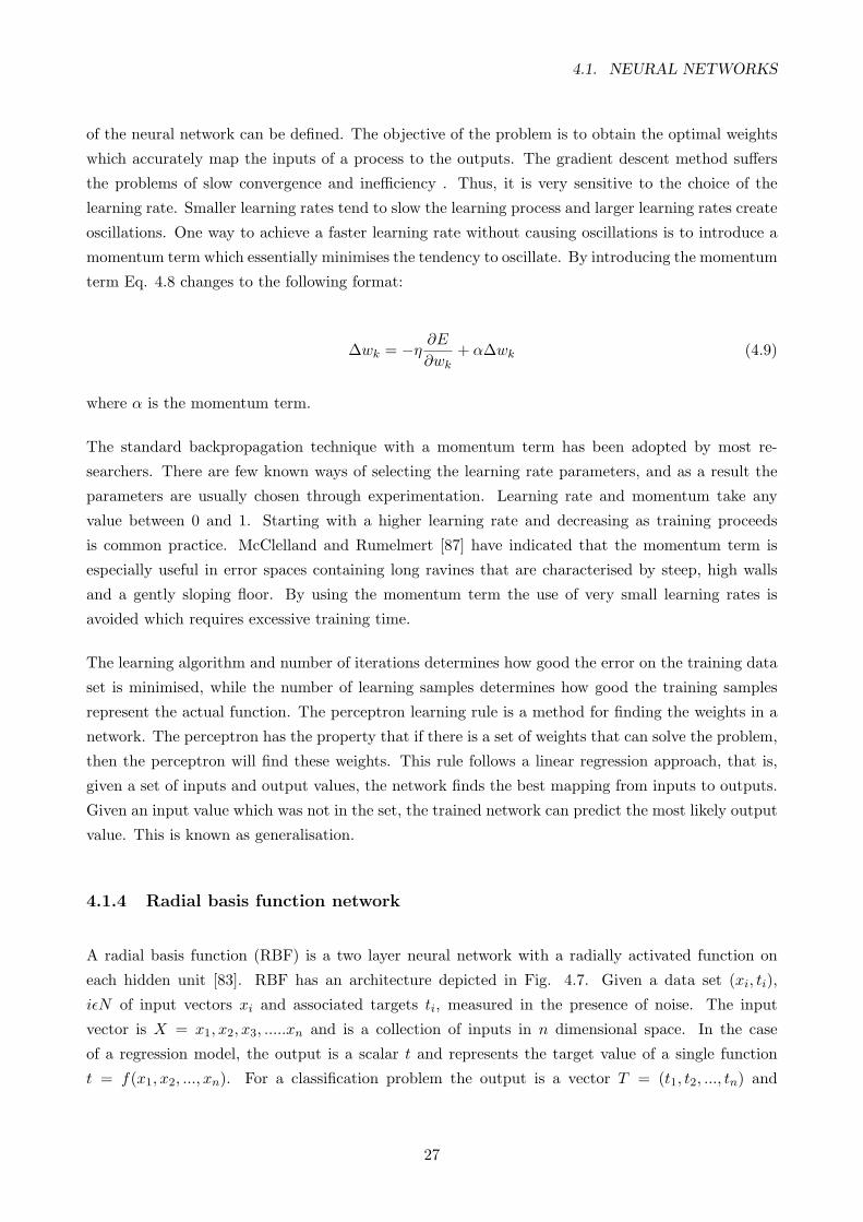
4.1. NEURAL NETWORKS
of the neural network can be defined. The objective of the problem is to obtain the optimal weights
which accurately map the inputs of a process to the outputs. The gradient descent method suffers
the problems of slow convergence and inefficiency . Thus, it is very sensitive to the choice of the
learning rate. Smaller learning rates tend to slow the learning process and larger learning rates create
oscillations. One way to achieve a faster learning rate without causing oscillations is to introduce a
momentum term which essentially minimises the tendency to oscillate. By introducing the momentum
term Eq. 4.8 changes to the following format:
∆wk = −η ∂E∂wk
+ α∆wk (4.9)
where α is the momentum term.
The standard backpropagation technique with a momentum term has been adopted by most re-
searchers. There are few known ways of selecting the learning rate parameters, and as a result the
parameters are usually chosen through experimentation. Learning rate and momentum take any
value between 0 and 1. Starting with a higher learning rate and decreasing as training proceeds
is common practice. McClelland and Rumelmert [87] have indicated that the momentum term is
especially useful in error spaces containing long ravines that are characterised by steep, high walls
and a gently sloping floor. By using the momentum term the use of very small learning rates is
avoided which requires excessive training time.
The learning algorithm and number of iterations determines how good the error on the training data
set is minimised, while the number of learning samples determines how good the training samples
represent the actual function. The perceptron learning rule is a method for finding the weights in a
network. The perceptron has the property that if there is a set of weights that can solve the problem,
then the perceptron will find these weights. This rule follows a linear regression approach, that is,
given a set of inputs and output values, the network finds the best mapping from inputs to outputs.
Given an input value which was not in the set, the trained network can predict the most likely output
value. This is known as generalisation.
4.1.4 Radial basis function network
A radial basis function (RBF) is a two layer neural network with a radially activated function on
each hidden unit [83]. RBF has an architecture depicted in Fig. 4.7. Given a data set (xi, ti),
iεN of input vectors xi and associated targets ti, measured in the presence of noise. The input
vector is X = x1, x2, x3, .....xn and is a collection of inputs in n dimensional space. In the case
of a regression model, the output is a scalar t and represents the target value of a single function
t = f(x1, x2, ..., xn). For a classification problem the output is a vector T = (t1, t2, ..., tn) and
27
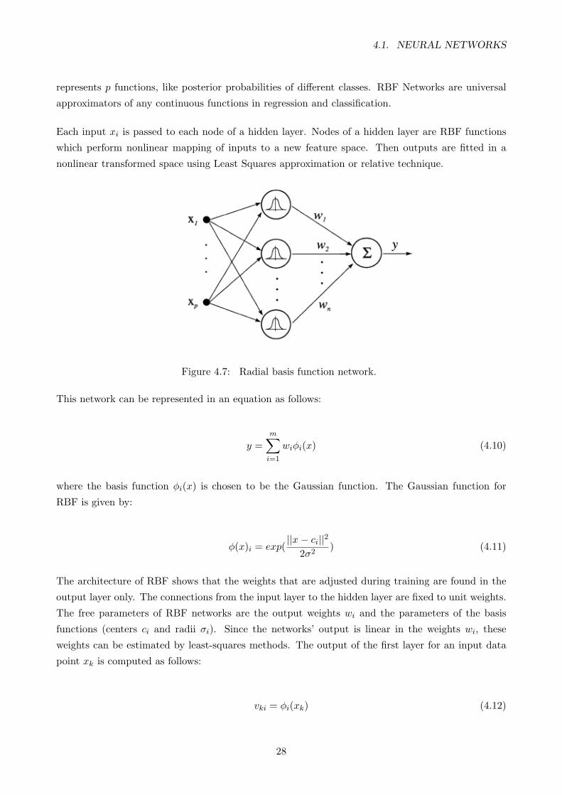
4.1. NEURAL NETWORKS
represents p functions, like posterior probabilities of different classes. RBF Networks are universal
approximators of any continuous functions in regression and classification.
Each input xi is passed to each node of a hidden layer. Nodes of a hidden layer are RBF functions
which perform nonlinear mapping of inputs to a new feature space. Then outputs are fitted in a
nonlinear transformed space using Least Squares approximation or relative technique.
Figure 4.7: Radial basis function network.
This network can be represented in an equation as follows:
y =m∑
i=1
wiφi(x) (4.10)
where the basis function φi(x) is chosen to be the Gaussian function. The Gaussian function for
RBF is given by:
φ(x)i = exp(||x− ci||2
2σ2) (4.11)
The architecture of RBF shows that the weights that are adjusted during training are found in the
output layer only. The connections from the input layer to the hidden layer are fixed to unit weights.
The free parameters of RBF networks are the output weights wi and the parameters of the basis
functions (centers ci and radii σi). Since the networks’ output is linear in the weights wi, these
weights can be estimated by least-squares methods. The output of the first layer for an input data
point xk is computed as follows:
vki = φi(xk) (4.12)
28
4.1. NEURAL NETWORKS
These outputs are then put into a matrix V =[vki]. The output of the first stage is then taken to the
next stage which involves the introduction of weights vector w = [w1, w2, ....wi]. The output of the
network can be written in the form of a matrix:
y∗ = V w (4.13)
The objective is to find a weight vector that will minimise the error between the actual output and
the output of the network, e = y∗ − y. To solve for w from Eq.4.13 a method of pseudo-inverse is
introduced because V may not be a square matrix and the equation is written as follows:
w = [V TV ]−1V T y∗ (4.14)
The adaptation of the RBF parameters ci and σi is a nonlinear optimisation problem that can be
solved by the gradient-descent method.
Training RBF
A training set is an m labelled pair (yi, ti) that represents associations of a given mapping or samples
of a continuous multivariate function. The sum of squared error criterion function can be considered
as an error function E to be minimised over the given training set. That is, to develop a training
method that minimises E by adaptively updating the free parameters of the RBF network. These
parameters are the receptive field centres ci of the hidden layer Gaussian units, the receptive field
widths σi, and the output layer weights (wij). Because of the differentiable nature of the RBF
network transfer characteristics, one of the training methods considered here was a fully supervised
gradient-descent method over E.
In particular, ci, σi and wij are updated as follows:
∆ci = −ρc∂E
∂ci(4.15)
∆σi = −ρσ∂E
∂σj(4.16)
∆wij = −ρw∂E
∂wij(4.17)
29
4.2. SUPPORT VECTOR MACHINES
where ρc, ρσ , and ρw are small positive constants. This method is capable of matching or exceeding
the performance of neural networks with back-propagation algorithms, but gives training comparable
with those of sigmoidal types of neural networks.
The training of the RBF network is radically different from the classical training of standard NNs.
In this case, there is no changing of weights with the use of the gradient method aimed at function
minimisation. In RBF networks with the chosen type of radial basis function, training resolves
itself into selecting the centres and dimensions of the functions and calculating the weights of the
output neuron. The centre, distance scale and precise shape of the radial function are parameters
of the model, all fixed if it is linear. Selection of the centres can be understood as defining the
optimal number of basis functions and choosing the elements of the training set used in the solution.
It was done according to the method of forward selection. Heuristic operation on a given defined
training set starts from an empty subset of the basis functions. Then the empty subset is filled with
succeeding basis functions with their centres marked by the location of elements of the training set;
which generally decreases the sum-squared error or the cost function. In this way, a model of the
network constructed each time is being completed by the best element. Construction of the network
is continued till the criterion demonstrating the quality of the model is fulfilled. The most commonly
used method for estimating generalisation error is the cross-validation error.
For the purpose of this work RBF is used to create a neuro-fuzzy model in combination with fuzzy
logic. The combination allows for the optimisation methods such as gradient descent methods from
the area of neural networks to be used to optimize parameters in a fuzzy system. A detailed expla-
nation can be found in section 4.3 of this chapter.
4.2 Support vector machines
Traditional neural network approaches have challenges of generalisation, and occasionally produce
models that can overfit the data. This is a consequence of the optimisation algorithms used to
select the model parameters and the statistical measures used to select the model that approximates
the relationship between the input and the output. The foundations of support vector machines
(SVM) have been developed by Vapnik [88] and are gaining popularity due to multiple attractive
features and promising empirical performance. SVM models are formulated using the Structural
Risk Minimisation (SRM) principle, which has been shown to be superior [89] to the traditional
Empirical Risk Minimisation (ERM) principle employed by the conventional neural networks. SRM
minimises the upper bound on the expected risk, as opposed to ERM which minimises the empirical
error on the training data. SRM equips SVM with a greater ability to generalise which is the goal of
statistical learning. SVMs were developed for solving classification problems, but recently they have
been extended to the domain of regression problems [90].
30
4.2. SUPPORT VECTOR MACHINES
4.2.1 Support vector machines classification
SVM uses linear models to implement nonlinear class boundaries through some nonlinear relationship
of mapping the input vectors x into the high-dimensional feature space. A linear model constructed
in the new space can represent a nonlinear decision boundary in the original space. In the new space,
an optimal separating hyperplane is constructed. Thus, SVM is known as the algorithm that finds
a special kind of linear model, the maximum margin hyperplane. The maximum margin hyperplane
gives the maximum separation between the decision classes. The training examples that are closest
to the maximum margin hyperplane are called support vectors. All other training examples are
irrelevant for defining the binary class boundaries. For the linearly separable case, a hyperplane
separating the binary decision classes in the three-attribute case can be represented as [90]:
y = w0 + w1x1 + w2x2 + w3x3 (4.18)
where y is the outcome, xi are the attribute values, and there are four weights wi to be learned by the
learning algorithm. In Eq. 4.18, the weights wi are parameters that determine the hyperplane. The
maximum margin hyperplane can be represented by the following equation in terms of the support
vectors [90]:
y = b+∑
αiyix (i) ·x (4.19)
where yi is the class value of training example x(i), · represents the dot product. The vector x
represents a test example and the vectors x(i) are the support vectors. In this equation, b and
αi are parameters that determine the hyperplane. From the implementation point of view, finding
the support vectors and determining the parameters b and αi are equivalent to solving a linearly
constrained quadratic programming (QP) problem. As mentioned above, SVM constructs a linear
model to implement nonlinear class boundaries by transforming the inputs into high-dimensional
feature space. For the nonlinearly separable case, a high-dimensional version of Eq. 4.19 is simply
represented as follows [90]:
y = b+∑
αiyiK (x (i) , x) (4.20)
The function K (x (i) , x) is defined as the kernel function. There are some different kernels for
generating the inner products to construct machines with different types of nonlinear decision surfaces
in the input space. Choosing among different kernels the model that minimises the estimate, one
chooses the best model. Common examples of the kernel function are the polynomial kernelK (x, y) =
(xy + 1)d and the Gaussian radial basis function K (x, y) = exp(−1/δ2 (x− y)2
)dwhere d is the
degree of the polynomial kernel and δ2 is the bandwidth of the Gaussian radial basis function kernel.
For the separable case, there is a lower bound 0 on the coefficient αi in Eq. 4.20. For the non-separable
case, SVM can be generalised by placing an upper bound C on the coefficients αi in addition to the
lower bound [90].
31
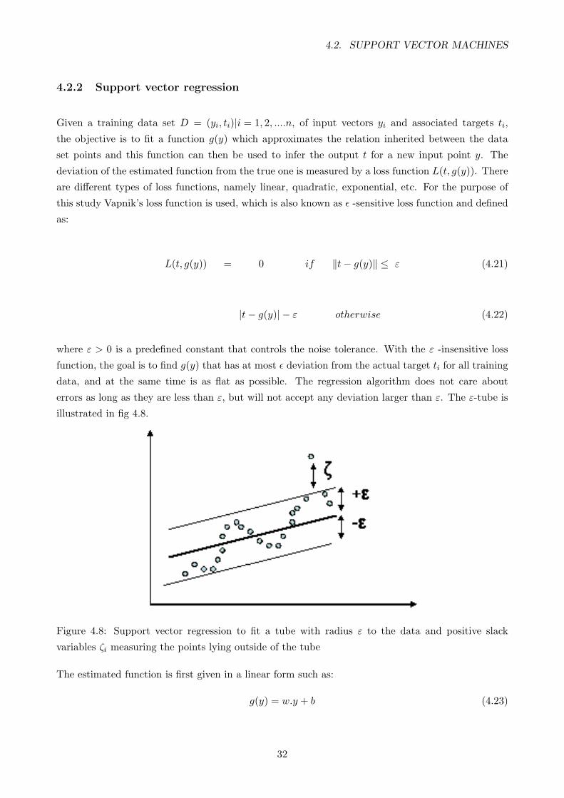
4.2. SUPPORT VECTOR MACHINES
4.2.2 Support vector regression
Given a training data set D = (yi, ti)|i = 1, 2, ....n, of input vectors yi and associated targets ti,
the objective is to fit a function g(y) which approximates the relation inherited between the data
set points and this function can then be used to infer the output t for a new input point y. The
deviation of the estimated function from the true one is measured by a loss function L(t, g(y)). There
are different types of loss functions, namely linear, quadratic, exponential, etc. For the purpose of
this study Vapnik’s loss function is used, which is also known as ε -sensitive loss function and defined
as:
L(t, g(y)) = 0 if ‖t− g(y)‖ ≤ ε (4.21)
|t− g(y)| − ε otherwise (4.22)
where ε > 0 is a predefined constant that controls the noise tolerance. With the ε -insensitive loss
function, the goal is to find g(y) that has at most ε deviation from the actual target ti for all training
data, and at the same time is as flat as possible. The regression algorithm does not care about
errors as long as they are less than ε, but will not accept any deviation larger than ε. The ε-tube is
illustrated in fig 4.8.
Figure 4.8: Support vector regression to fit a tube with radius ε to the data and positive slack
variables ζi measuring the points lying outside of the tube
The estimated function is first given in a linear form such as:
g(y) = w.y + b (4.23)
32
4.2. SUPPORT VECTOR MACHINES
The goal of a regression algorithm is to fit a flat function to the data points. Flatness in the case of
Eq. 4.23 means that one seeks a small w. One way to ensure this flatness is to minimise the norm,
i.e. ||w||2. Thus, the regression problem can be written as a convex optimisation problem:
minimise12||w||2 (4.24)
subject to ti − (w.y + b) ≤ ε and (4.25)
(w.y + b)− ti ≤ ε (4.26)
The implied assumption in Eq. 4.25 is that such a function g actually exists that approximates all
pairs (yi, ti) with ε precision, or in other words that the convex optimisation is feasible. Sometimes,
however, this may not be the case or we may want to allow some errors. Analogously to the “soft
margin” loss function [91] which was adapted to SVM machines by Vapnik [88], slack variables ζi, ζ∗ican be introduced to cope with otherwise infeasible constraints of the optimisation problem in Eq.
4.25 Hence the formulation stated in [88] is attained:
minimise12||w||2 + C
∑(ζi + ζ∗i ) (4.27)
subject to ti − (w.y + b) ≤ ε+ ζi (4.28)
(w.y + b)− ti ≤ ε+ ζ∗i (4.29)
ζi, ζ∗i ≥ 0 (4.30)
The constant C > 0 determines the trade-off between flatness of g and amount up to which deviations
larger than ε are tolerated. This corresponds to dealing with the so-called ε-sensitive loss function
which was described before.
It turns out that in most cases the optimisation problem Eq. 4.28 can be solved more easily in its
dual formulation. Moreover, the dual formulation provides the key for extending SVM to non-linear
functions.
33
4.2. SUPPORT VECTOR MACHINES
The minimisation problem in Eq. 4.28 is called the primal objective function. The basic idea
of the dual problem is to construct a Lagrange function from the primal objective function and
the corresponding constraints, by introducing a dual set of variables. It can be shown that the
Lagrange function has a saddle point with respect to the primal and dual variables at the solution
(see [92, 93]). The primal objective function with its constraints are transformed to the Lagrange
function. Hence the dual variables (Lagrange multipliers) from the Lagrange function have to satisfy
positivity constraints. This means that they have to be greater or equal to zero.
It follows from the saddle point condition that the partial derivatives of the Lagrange function with
respect to the primal variables (w, b, ζi, ζ∗i ) have to vanish for optimality. The outcomes of the partial
derivatives are then substituted into Eq. 4.24 to yield the dual optimisation problem:
maximise− 12
n∑i,j=1
(αi − α∗i )(αj − α∗j )(yi, y(j))− ε
n∑i=1
(α∗i + αi) +n∑
i=1
yi(αi − α∗i ) (4.31)
subject to
n∑i=1
yi(αi − α∗i ) = 0 and α∗i , αi ∈ [0, C] (4.32)
where α, α∗ are Lagrange multipliers. Eq. 4.23 can be rewritten as follows:
w =n∑
i=1
yi(αi − α∗i ), thus (4.33)
g(y) =n∑
i=1
(yi, y)(αi − α∗i ) + b (4.34)
This is called the Support Vector Regression Expansion, i.e. w can be completely described as a
linear combination of the training patterns yi.
In a sense, the complexity of a function’s representation by SVs is independent of the dimensionality
of the input space and depends only on the number of SVs.
Moreover, the complete algorithm can be described in terms of dot products between the data. Even
when evaluating g(y), the value of w does not need to be computed explicitly. These observations
will come in handy for the formulation of the nonlinear extension.
The Karush-Kuhn-Tucker (KKT) conditions [94][95] are the basics for the Lagrangian solution. These
conditions state that at the solution point, the product between dual variables and constraints has
to converge.
34
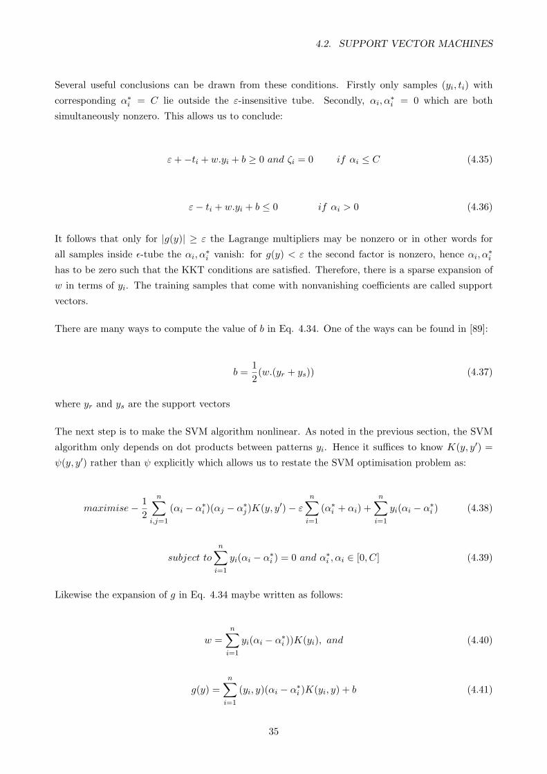
4.2. SUPPORT VECTOR MACHINES
Several useful conclusions can be drawn from these conditions. Firstly only samples (yi, ti) with
corresponding α∗i = C lie outside the ε-insensitive tube. Secondly, αi, α∗i = 0 which are both
simultaneously nonzero. This allows us to conclude:
ε+−ti + w.yi + b ≥ 0 and ζi = 0 if αi ≤ C (4.35)
ε− ti + w.yi + b ≤ 0 if αi > 0 (4.36)
It follows that only for |g(y)| ≥ ε the Lagrange multipliers may be nonzero or in other words for
all samples inside ε-tube the αi, α∗i vanish: for g(y) < ε the second factor is nonzero, hence αi, α
∗i
has to be zero such that the KKT conditions are satisfied. Therefore, there is a sparse expansion of
w in terms of yi. The training samples that come with nonvanishing coefficients are called support
vectors.
There are many ways to compute the value of b in Eq. 4.34. One of the ways can be found in [89]:
b =12(w.(yr + ys)) (4.37)
where yr and ys are the support vectors
The next step is to make the SVM algorithm nonlinear. As noted in the previous section, the SVM
algorithm only depends on dot products between patterns yi. Hence it suffices to know K(y, y′) =
ψ(y, y′) rather than ψ explicitly which allows us to restate the SVM optimisation problem as:
maximise− 12
n∑i,j=1
(αi − α∗i )(αj − α∗j )K(y, y′)− εn∑
i=1
(α∗i + αi) +n∑
i=1
yi(αi − α∗i ) (4.38)
subject ton∑
i=1
yi(αi − α∗i ) = 0 and α∗i , αi ∈ [0, C] (4.39)
Likewise the expansion of g in Eq. 4.34 maybe written as follows:
w =n∑
i=1
yi(αi − α∗i ))K(yi), and (4.40)
g(y) =n∑
i=1
(yi, y)(αi − α∗i )K(yi, y) + b (4.41)
35
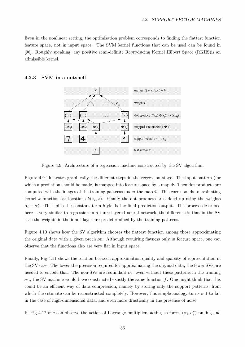
4.2. SUPPORT VECTOR MACHINES
Even in the nonlinear setting, the optimisation problem corresponds to finding the flattest function
feature space, not in input space. The SVM kernel functions that can be used can be found in
[96]. Roughly speaking, any positive semi-definite Reproducing Kernel Hilbert Space (RKHS)is an
admissible kernel.
4.2.3 SVM in a nutshell
Figure 4.9: Architecture of a regression machine constructed by the SV algorithm.
Figure 4.9 illustrates graphically the different steps in the regression stage. The input pattern (for
which a prediction should be made) is mapped into feature space by a map Φ. Then dot products are
computed with the images of the training patterns under the map Φ. This corresponds to evaluating
kernel k functions at locations k(xi, x). Finally the dot products are added up using the weights
αi − α∗i . This, plus the constant term b yields the final prediction output. The process described
here is very similar to regression in a three layered neural network, the difference is that in the SV
case the weights in the input layer are predetermined by the training patterns.
Figure 4.10 shows how the SV algorithm chooses the flattest function among those approximating
the original data with a given precision. Although requiring flatness only in feature space, one can
observe that the functions also are very flat in input space.
Finally, Fig 4.11 shows the relation between approximation quality and sparsity of representation in
the SV case. The lower the precision required for approximating the original data, the fewer SVs are
needed to encode that. The non-SVs are redundant i.e. even without these patterns in the training
set, the SV machine would have constructed exactly the same function f . One might think that this
could be an efficient way of data compression, namely by storing only the support patterns, from
which the estimate can be reconstructed completely. However, this simple analogy turns out to fail
in the case of high-dimensional data, and even more drastically in the presence of noise.
In Fig 4.12 one can observe the action of Lagrange multipliers acting as forces (αi, α∗i ) pulling and
36
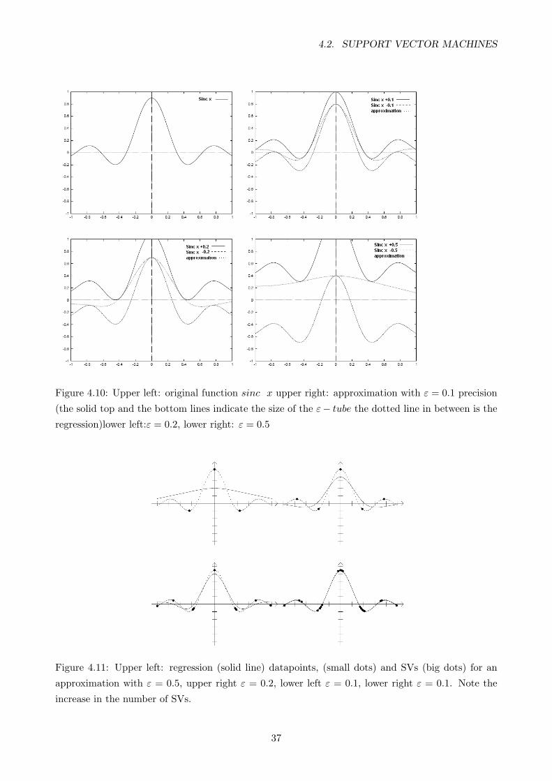
4.2. SUPPORT VECTOR MACHINES
Figure 4.10: Upper left: original function sinc x upper right: approximation with ε = 0.1 precision
(the solid top and the bottom lines indicate the size of the ε− tube the dotted line in between is the
regression)lower left:ε = 0.2, lower right: ε = 0.5
Figure 4.11: Upper left: regression (solid line) datapoints, (small dots) and SVs (big dots) for an
approximation with ε = 0.5, upper right ε = 0.2, lower left ε = 0.1, lower right ε = 0.1. Note the
increase in the number of SVs.
37
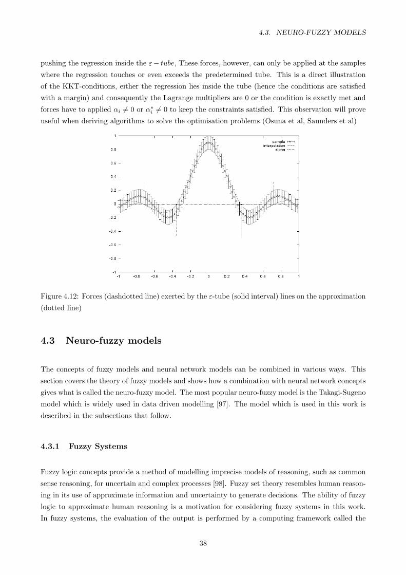
4.3. NEURO-FUZZY MODELS
pushing the regression inside the ε− tube, These forces, however, can only be applied at the samples
where the regression touches or even exceeds the predetermined tube. This is a direct illustration
of the KKT-conditions, either the regression lies inside the tube (hence the conditions are satisfied
with a margin) and consequently the Lagrange multipliers are 0 or the condition is exactly met and
forces have to applied αi 6= 0 or α∗i 6= 0 to keep the constraints satisfied. This observation will prove
useful when deriving algorithms to solve the optimisation problems (Osuna et al, Saunders et al)
Figure 4.12: Forces (dashdotted line) exerted by the ε-tube (solid interval) lines on the approximation
(dotted line)
4.3 Neuro-fuzzy models
The concepts of fuzzy models and neural network models can be combined in various ways. This
section covers the theory of fuzzy models and shows how a combination with neural network concepts
gives what is called the neuro-fuzzy model. The most popular neuro-fuzzy model is the Takagi-Sugeno
model which is widely used in data driven modelling [97]. The model which is used in this work is
described in the subsections that follow.
4.3.1 Fuzzy Systems
Fuzzy logic concepts provide a method of modelling imprecise models of reasoning, such as common
sense reasoning, for uncertain and complex processes [98]. Fuzzy set theory resembles human reason-
ing in its use of approximate information and uncertainty to generate decisions. The ability of fuzzy
logic to approximate human reasoning is a motivation for considering fuzzy systems in this work.
In fuzzy systems, the evaluation of the output is performed by a computing framework called the
38

4.3. NEURO-FUZZY MODELS
fuzzy inference system. The fuzzy inference system maps fuzzy or crisp inputs to the output - which
is usually a fuzzy set [99]. The fuzzy inference system performs a composition of the inputs using
fuzzy set theory, fuzzy if-then rules and fuzzy reasoning to arrive at the output. More specifically,
the fuzzy inference involves the fuzzification of the input variables (i.e. partitioning of the input
data into fuzzy sets), evaluation of rules, aggregation of the rule outputs and finally the defuzzifi-
cation (i.e. extraction of a crisp value which best represents a fuzzy set) of the result. There are
two popular fuzzy models: the Mamdani model and the Takagi-Sugeno (TS) model. The TS model
is more popular when it comes to data-driven identification and has been proven to be a universal
approximator [99].
A fuzzy model is a mathematical model that in some way uses fuzzy sets. The models are premised
on rule based system identification. The if-then rules, with imprecise predicates, are the means used
to represent relationships between variables such as:
If the percentage increase of an asset price today is high then tomorrow’s percentage increase will
be medium
For the representation to be operational, terms ‘high’ and ‘medium’ need to be defined more precisely.
The definition of these terms can be represented with fuzzy sets that have membership that gradually
changes. Fuzzy sets are defined through their membership functions (denoted by µ) which map the
elements of the considered space to the unit interval [0, 1]. The extreme values 0 and 1 denote
complete membership and non-membership, respectively, while a degree between 0 and 1 means
partial membership in the fuzzy set. Depending on the structure of the if-then rules, two main types
of fuzzy models can be distinguished: the Mamdani (or linguistic) model and the Takagi-Sugeno
model.
4.3.2 Mamdani models
The Mamdani fuzzy model is a modelling technique that is typically used in knowledge-based or
expert systems. The reason for this is that the model is a linguistic fuzzy model that is very useful
in representing qualitative knowledge, illustrated in the following example: Consider a qualitative
description of the relationship between the oxygen supply to a gas burner (x) and its heating power
(y).
If O2 flow rate is Low then power is Low (4.42)
39
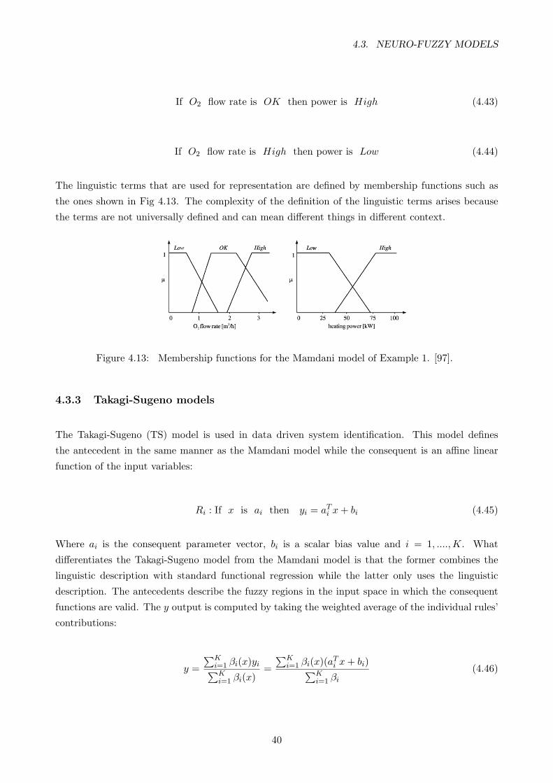
4.3. NEURO-FUZZY MODELS
If O2 flow rate is OK then power is High (4.43)
If O2 flow rate is High then power is Low (4.44)
The linguistic terms that are used for representation are defined by membership functions such as
the ones shown in Fig 4.13. The complexity of the definition of the linguistic terms arises because
the terms are not universally defined and can mean different things in different context.
Figure 4.13: Membership functions for the Mamdani model of Example 1. [97].
4.3.3 Takagi-Sugeno models
The Takagi-Sugeno (TS) model is used in data driven system identification. This model defines
the antecedent in the same manner as the Mamdani model while the consequent is an affine linear
function of the input variables:
Ri : If x is ai then yi = aTi x+ bi (4.45)
Where ai is the consequent parameter vector, bi is a scalar bias value and i = 1, ....,K. What
differentiates the Takagi-Sugeno model from the Mamdani model is that the former combines the
linguistic description with standard functional regression while the latter only uses the linguistic
description. The antecedents describe the fuzzy regions in the input space in which the consequent
functions are valid. The y output is computed by taking the weighted average of the individual rules’
contributions:
y =∑K
i=1 βi(x)yi∑Ki=1 βi(x)
=∑K
i=1 βi(x)(aTi x+ bi)∑K
i=1 βi
(4.46)
40
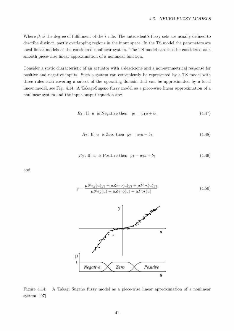
4.3. NEURO-FUZZY MODELS
Where βi is the degree of fulfillment of the i rule. The antecedent’s fuzzy sets are usually defined to
describe distinct, partly overlapping regions in the input space. In the TS model the parameters are
local linear models of the considered nonlinear system. The TS model can thus be considered as a
smooth piece-wise linear approximation of a nonlinear function.
Consider a static characteristic of an actuator with a dead-zone and a non-symmetrical response for
positive and negative inputs. Such a system can conveniently be represented by a TS model with
three rules each covering a subset of the operating domain that can be approximated by a local
linear model, see Fig. 4.14. A Takagi-Sugeno fuzzy model as a piece-wise linear approximation of a
nonlinear system and the input-output equation are:
R1 : If u is Negative then y1 = a1u+ b1 (4.47)
R2 : If u is Zero then y2 = a2u+ b2 (4.48)
R3 : If u is Positive then y3 = a3u+ b3 (4.49)
and
y =µNeg(u)y1 + µZero(u)y2 + µPos(u)y3
µNeg(u) + µZero(u) + µPos(u)(4.50)
Figure 4.14: A Takagi Sugeno fuzzy model as a piece-wise linear approximation of a nonlinear
system. [97].
41
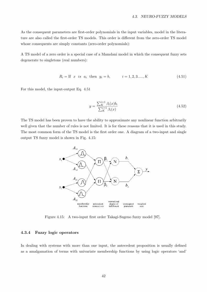
4.3. NEURO-FUZZY MODELS
As the consequent parameters are first-order polynomials in the input variables, model in the litera-
ture are also called the first-order TS models. This order is different from the zero-order TS model
whose consequents are simply constants (zero-order polynomials):
A TS model of a zero order is a special case of a Mamdani model in which the consequent fuzzy sets
degenerate to singletons (real numbers):
Ri = If x is ai then yi = b, i = 1, 2, 3.....,K (4.51)
For this model, the input-output Eq. 4.51
y =∑i=1
K βi(x)bi∑i=1K βi(x)
(4.52)
The TS model has been proven to have the ability to approximate any nonlinear function arbitrarily
well given that the number of rules is not limited. It is for these reasons that it is used in this study.
The most common form of the TS model is the first order one. A diagram of a two-input and single
output TS fuzzy model is shown in Fig. 4.15:
Figure 4.15: A two-input first order Takagi-Sugeno fuzzy model [97].
4.3.4 Fuzzy logic operators
In dealing with systems with more than one input, the antecedent proposition is usually defined
as a amalgamation of terms with univariate membership functions by using logic operators ‘and’
42
4.3. NEURO-FUZZY MODELS
(conjuction), ‘or’ (disjunction), and ‘not’ (complement). As an example, consider the conjunctive
form of the antecedent,which is given by:
Ri = If x1 is Ai1 and...and xp is Aip then yi = aTi x+ bi (4.53)
with a degree of fulfillment
βi(x) = min(µAi1(xi), ...., µAip(xp)) (4.54)
4.3.5 Fuzzy to Neuro-fuzzy
Fuzzy logic limits the membership functions and the consequent models to a priori knowledge of
the model designer. The adaptive neuro-fuzzy inference system (ANFIS) is an architecture which is
functionally equivalent to a Sugeno type fuzzy rule base [100]. Under certain minor constraints the
ANFIS architecture is also equivalent to a radial basis function network [101]. In a loose kind of way
ANFIS is a method for tuning an existing rule base with a learning algorithm based on a collection of
training data. What differentiates neuro-fuzzy modelling from fuzzy logic is that in the absence of the
knowledge and the availability of the input-output data observed from the process, the components
of the fuzzy system membership and consequent models can be represented in a parametric form and
the parameters tuned by a learning procedure as shown in its architecture in Fig. 4.16. In this case
the fuzzy system turns into a neuro fuzzy approximator. Neuro-fuzzy systems combine human-like
representation and the fast learning methods used in neural networks and therefore have a tradeoff
in terms of readability and efficiency. However, what mainly distinguishes neuro-fuzzy estimators
from other kinds of non linear approximators is their potentiality for combining available a priori
first principle models with data driven modelling techniques.
4.3.6 Neuro-fuzzy learning procedure
In a neuro-fuzzy system, there are two types of model tuning which are required, namely structural
and parametric tuning.
Structural tuning is a procedure that finds the suitable number of rules and the proper partitioning of
the input space. Upon finding the suitable structure, the parametric tuning searches for the optimal
membership functions together with the optimal parameters of the consequent models. The problem
can be formulated as that of finding the structure complexity which will give the best performance
in generalisation. The structure selection involves the following two choices:
43
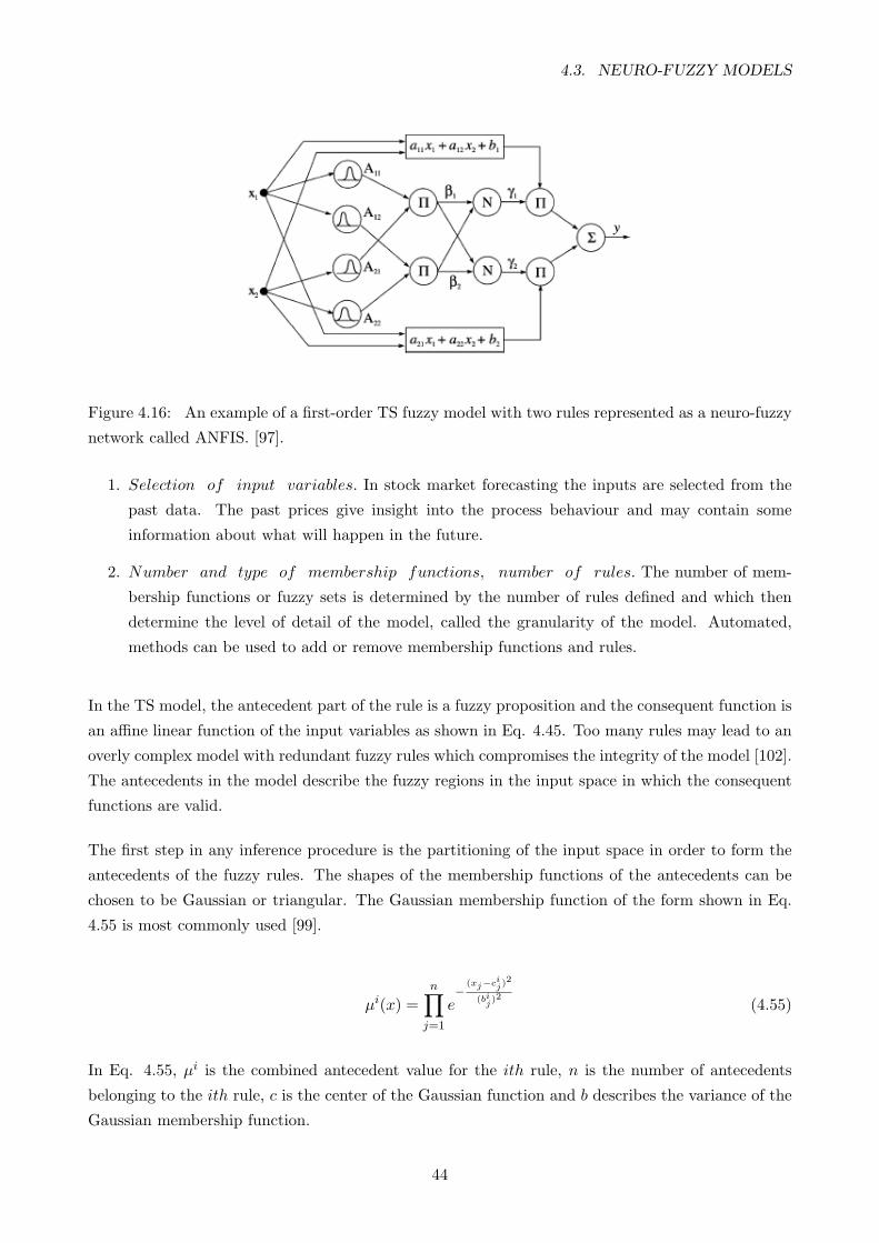
4.3. NEURO-FUZZY MODELS
Figure 4.16: An example of a first-order TS fuzzy model with two rules represented as a neuro-fuzzy
network called ANFIS. [97].
1. Selection of input variables. In stock market forecasting the inputs are selected from the
past data. The past prices give insight into the process behaviour and may contain some
information about what will happen in the future.
2. Number and type of membership functions, number of rules. The number of mem-
bership functions or fuzzy sets is determined by the number of rules defined and which then
determine the level of detail of the model, called the granularity of the model. Automated,
methods can be used to add or remove membership functions and rules.
In the TS model, the antecedent part of the rule is a fuzzy proposition and the consequent function is
an affine linear function of the input variables as shown in Eq. 4.45. Too many rules may lead to an
overly complex model with redundant fuzzy rules which compromises the integrity of the model [102].
The antecedents in the model describe the fuzzy regions in the input space in which the consequent
functions are valid.
The first step in any inference procedure is the partitioning of the input space in order to form the
antecedents of the fuzzy rules. The shapes of the membership functions of the antecedents can be
chosen to be Gaussian or triangular. The Gaussian membership function of the form shown in Eq.
4.55 is most commonly used [99].
µi(x) =n∏
j=1
e−
(xj−cij)2
(bij)2 (4.55)
In Eq. 4.55, µi is the combined antecedent value for the ith rule, n is the number of antecedents
belonging to the ith rule, c is the center of the Gaussian function and b describes the variance of the
Gaussian membership function.
44

4.3. NEURO-FUZZY MODELS
The output y of the entire inference system is computed by taking a weighted average of the individual
rules’ contributions as shown in Eq. 4.46 [99]. The parameters obtained from the training are then
used to approximate models of the non-linear system under consideration [103].
4.3.7 Neuro-fuzzy modelling
When setting up a fuzzy rule-based system we are required to optimise parameters such as member-
ship functions and consequent parameters. At the computational level, a fuzzy system can be seen
as a layered structure (network), similar to artificial neural networks of the RBF-type [101]. In order
to optimise these parameters, the fuzzy system relies on training algorithms inherited from artificial
neural networks such as gradient descent-based learning. It is for this reason that they are referred
to as neuro-fuzzy models. There are two approaches to constructing neuro-fuzzy models [97]:
1. Fuzzy rules may be extracted from expert knowledge and used to create an initial model. The
parameters of the model can then be fine tuned using data collected from the operational system
being modeled.
2. The number of rules can be determined from collected numerical data using a model selection
technique. The parameters of the model are also optimised using the existing data. The
Takagi-Sugeno model is most popular when it comes to this identification technique.
4.3.8 Neuro-fuzzy learning algorithm
Fixing the premise parameters of the Neuro-fuzzy ANFIS model makes the overall output combination
linear . A hybrid algorithm adjusts the consequent parameters of the model in a forward pass and
the premise parameters of the model in a backward pass [101]. In the forward pass the network
inputs propagate forward until the output layer of the network, where the consequent parameters are
identified by the least-squares method. In the backward pass, the error signals propagate backwards
and the premise parameters are updated by gradient descent.
Because the update rules for the premise and consequent parameters are decoupled in the hybrid
learning rule, a computational speedup may be possible by using variants of the gradient method
or other optimisation techniques on the premise parameters. Since ANFIS and radial basis function
networks (RBFNs) are functionally equivalent under some minor conditions, a variety of learning
methods can be used for both of them.
45
4.3. NEURO-FUZZY MODELS
4.3.9 Clustering of data
In order to set up a Takagi-Sugeno model of a system, it is important to have an automatic method
that finds clusters in the data that would form the linear regions. The objective of such a cluster
analysis is to partition the data set into a number of natural and homogeneous subsets, where the
elements of each subset are as similar to each other as possible, and at the same time as different
from those of the other sets as possible. Clusters are such a grouping of objects, that is, it consists
of all points close, in some sense, to the cluster centre.
(a) Hard clusters
The Hard c-means algorithm attempts to locate clusters of data with a multidimensional feature
space . The basic approach of the algorithm is as follows [104]:
1. The algorithm is manually seeded with c cluster centres, one for each cluster. This turns the
algorithm into supervised learning because information about the number of different clusters
is already known.
2. Each point is assigned to the cluster centre nearest to it.
3. A new cluster centre is computed for each class by taking the mean values of the coordinates
of the points assigned to it.
4. If not finished according to some stopping criterion, go to step 2.
(b) Fuzzy clusters
The fuzzified c-means algorithm [106] allows each data point to belong to a cluster to a degree
specified by a membership grade, and thus each point may belong to several clusters. The fuzzy
c-means (FCM) algorithm partitions a collection of N data points specified by p-dimensional vectors
uk(k = 1, 2, ....,K), into f fuzzy clusters, and finds a cluster centre. Fuzzy c-means is different
from hard c-means (HFC), mainly because it employs fuzzy partitioning where a point can belong to
several clusters with degrees of membership. To accommodate the fuzzy partitioning, the membership
matrix M is allowed to have elements in the range [0, 1]. A points total membership of all clusters,
however, must always be equal to unity to maintain the properties of the M matrix.
46

4.3. NEURO-FUZZY MODELS
(c) Gustatson-Kessel algorithm
The Gustatson-Kessel (GK) algorithm is an extension of the standard fuzzy c-means algorithm by
employing an adaptive distance norm in order to detect clusters of different geometric shapes in one
data set [105]. The GK algorithm basically contains four steps. Step 1 is computation of cluster
prototypes or means. Step 2 then calculates the cluster covariance matrices. Step 3 then calculates
the cluster distances. Step 4 then updates the partition matrix. The algorithm then iterates through
these steps until the change in membership degrees is less than a given tolerance. For a more detailed
explanation of the algorithm refer to appendix A.
The advantages of using the GK algorithm are listed below:
• The resulting fuzzy sets induced by the partition matrix are compact and are therefore easy to
interprete.
• In comparison to other clustering algorithms, the GK algorithm is relatively insensitive to the
initialisations of the partition matrix.
• The algorithm is based on an adaptive distance measure and is therefore less sensitive to the
normalisation of the data.
• The GK algorithm can detect clusters of different shapes, i.e., not only linear subspaces.
47
Chapter 5
Auto-Regressive Moving Average Modelling
5.1 Introduction
Auto-Regressive Moving Average (ARMA) model is a Box-Jenkins model that combines Auto-
Regression (AR) and Moving Average (MA). AR model is simply a linear regression of the current
value of a time series against one or more prior values of the series. MA model is a linear regression
of the current value of the series against the white noise or random shocks of one or more prior
values of a time series. Box and Jenkins popularized an approach that combines the moving average
and the autoregressive approaches in the book, Time Series Analysis: Forecasting and Control [34].
The Box-Jenkins models are useful for the representation of processes that are stationary or non-
stationary. The statistical properties of a stationary time series are the same over time; in particular,
the mean of such a time series is fixed and a non-stationary time series changes in level, trends, etc.
This chapter starts with the description of the mathematical modelling of the ARMA model and
then describes how a model is constructed to forecast a stock market index.
5.2 Mathematical model
ARMA model is represented by a series of equations. These equations combine the autoregressive
(AR) equation and moving average (MA) equation. Autoregressive models are based on the con-
cept that the current value of the time series, xt, can be explained as a function of p past values,
xt−1, xt−2, ..., xt−p, where p determines the number of periods into the past selected to forecast the
current value. The equations are simplified by first reducing the time series to zero-mean and so
doing the sample mean is subtracted. The series is mean adjusted as follows:
xadjusted = x− xmean (5.1)
48
5.2. MATHEMATICAL MODEL
where x is the original time series, xmean is its sample mean, and xadjusted is the mean-adjusted series.
An AR model expresses a time series as a linear function of its past values. The order of the AR
model is the number of lagged past values that should be included in the model. The simplest AR
model is the model with only one lagged past value which is the first-order autoregressive, or AR(1),
model
xt + a1xt−1 = et (5.2)
where xt is the mean-adjusted series in day t, xt−1 is the series in the previous day, a1 is the lag-1
autoregressive coefficient, and et is the noise parameter. The noise can also be referred to as the
error, the random-shock, and the residual. The residuals et are assumed to be occurring randomoly
in time or white noise (not autocorrelated), and to have a Gaussian distribution. By rewriting the
equation for the AR(1) model as
xt = −a1xt−1 + et (5.3)
illustrates that the AR(1) model has the form of a regression model in which xt is regressed on its
previous value. In this form, a1 is analogous to the regression coefficient, and et to the regression
residuals.
Higher-order autoregressive models include more lagged xt terms as predictors. For example, the
third-order autoregressive model, AR(3), is given by
xt + a1xt−1 + a2xt−2 + a3xt−3 = et (5.4)
where a1, a2, a3 are the autoregressive coefficients on lags 1,2 and 3. The pth order autoregressive
model, AR(p) includes lagged terms on years t -1 to t - p .
The moving average (MA) model is another subset of the ARMA model in which the time series
is regarded as a moving average (unevenly weighted) of a random shock series et . The first-order
moving average, or MA(1), model is given by
xt = et + c1et−1 (5.5)
where et, et−1 are the residuals at times t and t−1, and c is the first-order moving average coefficient.
As with the AR models, higher-order MA models include higher lagged terms. For example, the
49
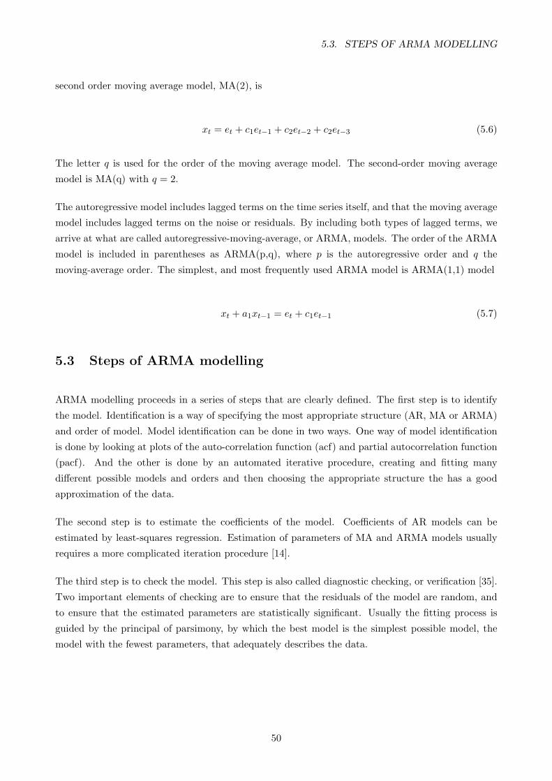
5.3. STEPS OF ARMA MODELLING
second order moving average model, MA(2), is
xt = et + c1et−1 + c2et−2 + c2et−3 (5.6)
The letter q is used for the order of the moving average model. The second-order moving average
model is MA(q) with q = 2.
The autoregressive model includes lagged terms on the time series itself, and that the moving average
model includes lagged terms on the noise or residuals. By including both types of lagged terms, we
arrive at what are called autoregressive-moving-average, or ARMA, models. The order of the ARMA
model is included in parentheses as ARMA(p,q), where p is the autoregressive order and q the
moving-average order. The simplest, and most frequently used ARMA model is ARMA(1,1) model
xt + a1xt−1 = et + c1et−1 (5.7)
5.3 Steps of ARMA modelling
ARMA modelling proceeds in a series of steps that are clearly defined. The first step is to identify
the model. Identification is a way of specifying the most appropriate structure (AR, MA or ARMA)
and order of model. Model identification can be done in two ways. One way of model identification
is done by looking at plots of the auto-correlation function (acf) and partial autocorrelation function
(pacf). And the other is done by an automated iterative procedure, creating and fitting many
different possible models and orders and then choosing the appropriate structure the has a good
approximation of the data.
The second step is to estimate the coefficients of the model. Coefficients of AR models can be
estimated by least-squares regression. Estimation of parameters of MA and ARMA models usually
requires a more complicated iteration procedure [14].
The third step is to check the model. This step is also called diagnostic checking, or verification [35].
Two important elements of checking are to ensure that the residuals of the model are random, and
to ensure that the estimated parameters are statistically significant. Usually the fitting process is
guided by the principal of parsimony, by which the best model is the simplest possible model, the
model with the fewest parameters, that adequately describes the data.
50
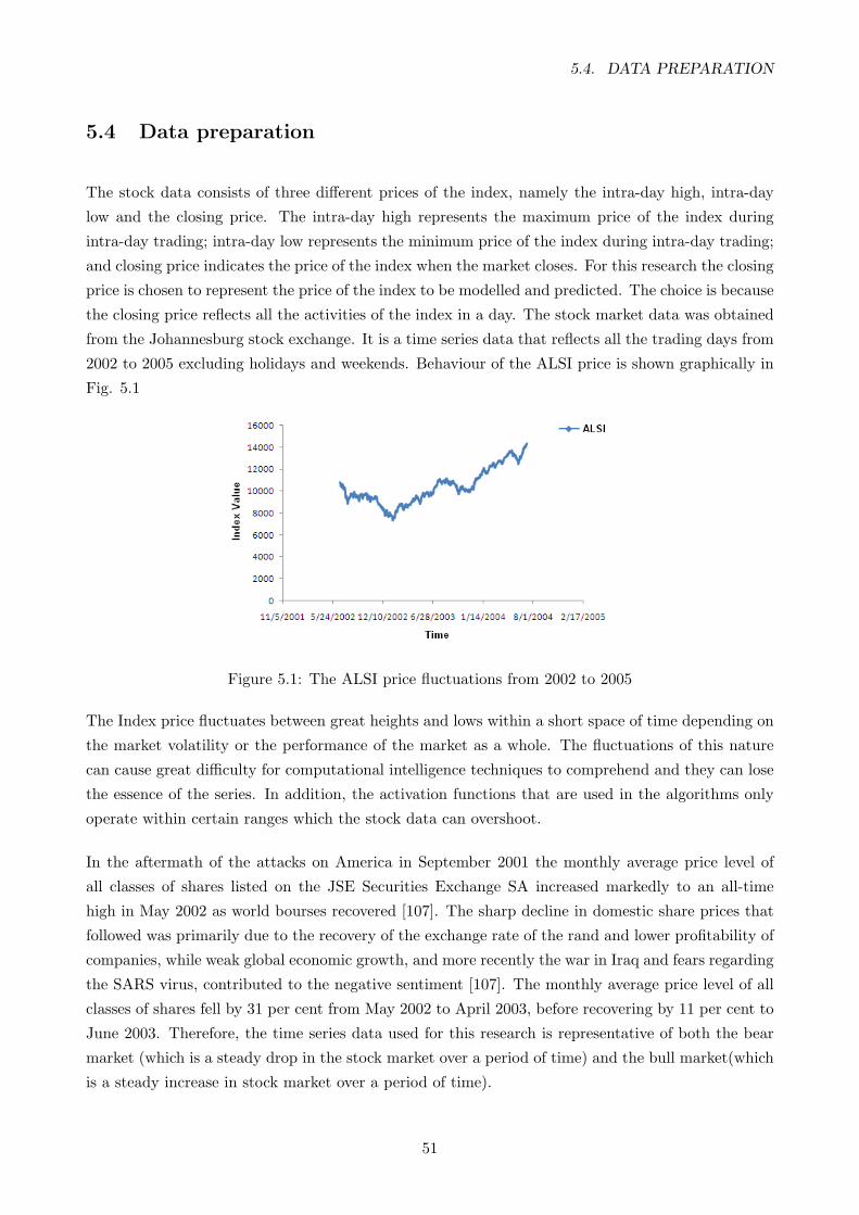
5.4. DATA PREPARATION
5.4 Data preparation
The stock data consists of three different prices of the index, namely the intra-day high, intra-day
low and the closing price. The intra-day high represents the maximum price of the index during
intra-day trading; intra-day low represents the minimum price of the index during intra-day trading;
and closing price indicates the price of the index when the market closes. For this research the closing
price is chosen to represent the price of the index to be modelled and predicted. The choice is because
the closing price reflects all the activities of the index in a day. The stock market data was obtained
from the Johannesburg stock exchange. It is a time series data that reflects all the trading days from
2002 to 2005 excluding holidays and weekends. Behaviour of the ALSI price is shown graphically in
Fig. 5.1
Figure 5.1: The ALSI price fluctuations from 2002 to 2005
The Index price fluctuates between great heights and lows within a short space of time depending on
the market volatility or the performance of the market as a whole. The fluctuations of this nature
can cause great difficulty for computational intelligence techniques to comprehend and they can lose
the essence of the series. In addition, the activation functions that are used in the algorithms only
operate within certain ranges which the stock data can overshoot.
In the aftermath of the attacks on America in September 2001 the monthly average price level of
all classes of shares listed on the JSE Securities Exchange SA increased markedly to an all-time
high in May 2002 as world bourses recovered [107]. The sharp decline in domestic share prices that
followed was primarily due to the recovery of the exchange rate of the rand and lower profitability of
companies, while weak global economic growth, and more recently the war in Iraq and fears regarding
the SARS virus, contributed to the negative sentiment [107]. The monthly average price level of all
classes of shares fell by 31 per cent from May 2002 to April 2003, before recovering by 11 per cent to
June 2003. Therefore, the time series data used for this research is representative of both the bear
market (which is a steady drop in the stock market over a period of time) and the bull market(which
is a steady increase in stock market over a period of time).
51
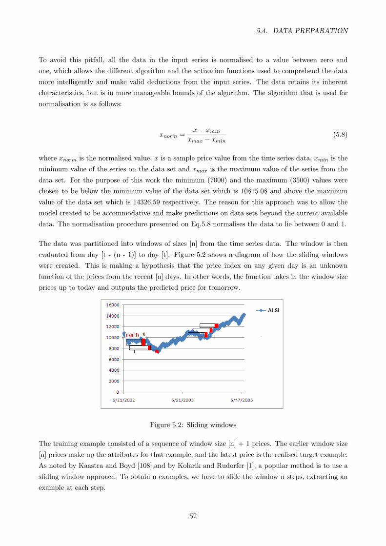
5.4. DATA PREPARATION
To avoid this pitfall, all the data in the input series is normalised to a value between zero and
one, which allows the different algorithm and the activation functions used to comprehend the data
more intelligently and make valid deductions from the input series. The data retains its inherent
characteristics, but is in more manageable bounds of the algorithm. The algorithm that is used for
normalisation is as follows:
xnorm =x− xmin
xmax − xmin(5.8)
where xnorm is the normalised value, x is a sample price value from the time series data, xmin is the
minimum value of the series on the data set and xmax is the maximum value of the series from the
data set. For the purpose of this work the minimum (7000) and the maximum (3500) values were
chosen to be below the minimum value of the data set which is 10815.08 and above the maximum
value of the data set which is 14326.59 respectively. The reason for this approach was to allow the
model created to be accommodative and make predictions on data sets beyond the current available
data. The normalisation procedure presented on Eq.5.8 normalises the data to lie between 0 and 1.
The data was partitioned into windows of sizes [n] from the time series data. The window is then
evaluated from day [t - (n - 1)] to day [t]. Figure 5.2 shows a diagram of how the sliding windows
were created. This is making a hypothesis that the price index on any given day is an unknown
function of the prices from the recent [n] days. In other words, the function takes in the window size
prices up to today and outputs the predicted price for tomorrow.
Figure 5.2: Sliding windows
The training example consisted of a sequence of window size [n] + 1 prices. The earlier window size
[n] prices make up the attributes for that example, and the latest price is the realised target example.
As noted by Kaastra and Boyd [108],and by Kolarik and Rudorfer [1], a popular method is to use a
sliding window approach. To obtain n examples, we have to slide the window n steps, extracting an
example at each step.
52
5.5. PERFORMANCE MEASURE
The data was then partitioned into training and testing data. Training data of 500 points ranging
from 2002 through to 2004 and testing data of about 200 points ranging from 2004 to 2005 was
used for the experiment. Figure 5.3 shows the dates in which the data was partitioned to create the
training and the testing data.
Figure 5.3: A diagram showing the dates of the partitioning of the training and testing data
5.5 Performance measure
An important part of financial prediction is the evaluation of the prediction algorithm. Several perfor-
mance measures are widely used, but a performance measure in itself is not sufficient for a satisfying
evaluation. Relevant benchmarks are also needed. A benchmark is basically a different prediction
algorithm used for comparison. This section gives an overview of the performance measurement tools
used for this experiment.
Research teaches three lessons about averaging over a series, according to Tashman [10]:
1. The use of scale dependent error measures should be avoided. This includes error measures
such as root mean square error RMSE or mean absolute deviation MAD. Changing the scale
of the measurement, alters the error measure also. Larger deviations may dominate the error
measures.
2. Percent error measures such as absolute percent error should be used because they are scale
independent. However, percent measures have their own shortcomings, the distribution of the
percent errors can be badly skewed, especially if the series contains values close to zero.
3. Relative error measures can be used if it is necessary to average over time series that differ in
volatility.
Various accuracy measurement methods were used to avoid some of the pitfalls that have already
been highlighted about some of the methods and they were selected because of their diversity. These
methods include, mean absolute percentage error (MAPE), symmetrical mean absolute percentage
error (sMAPE), mean squared error (MSE), root mean squared error (RMSE) and mean squared
relative error (MSRE). For details on the methods see appendix C.
53
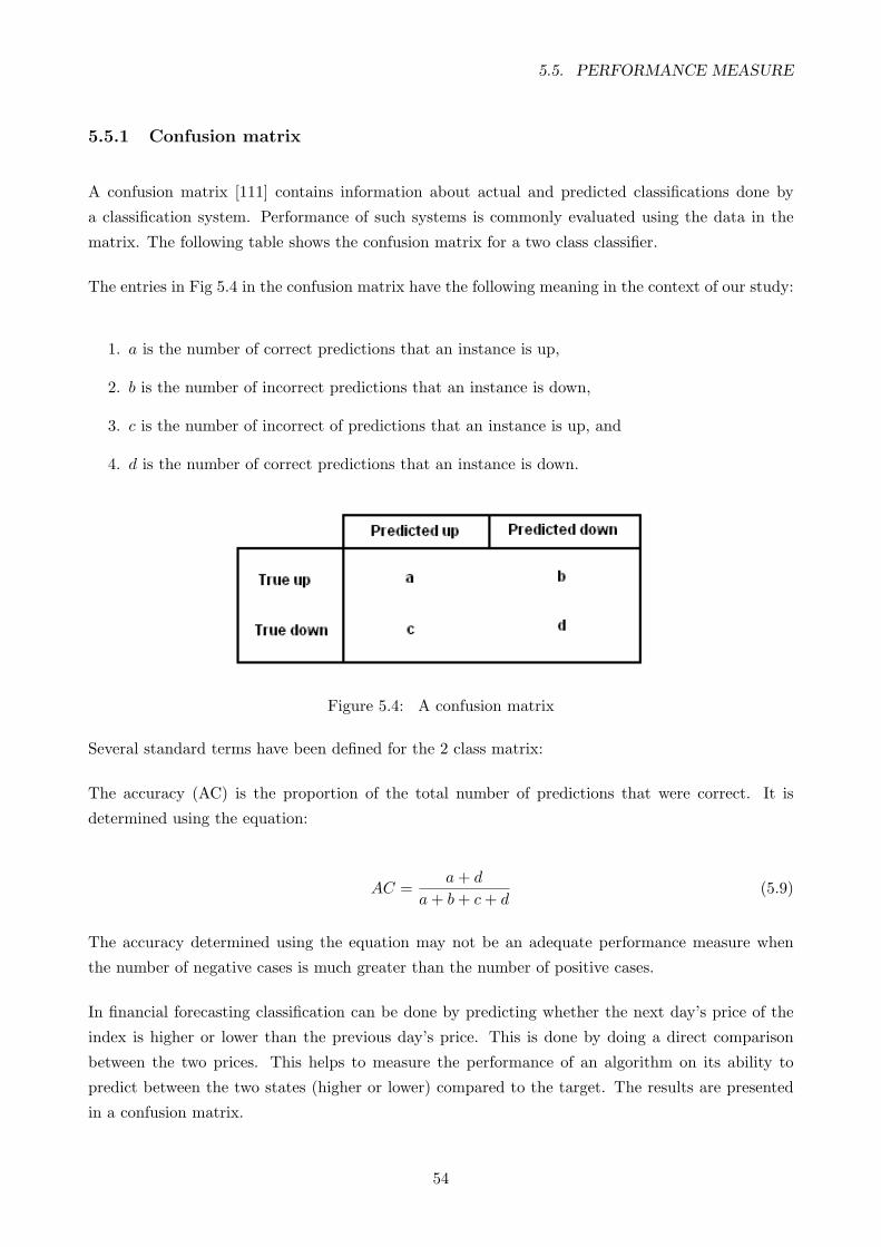
5.5. PERFORMANCE MEASURE
5.5.1 Confusion matrix
A confusion matrix [111] contains information about actual and predicted classifications done by
a classification system. Performance of such systems is commonly evaluated using the data in the
matrix. The following table shows the confusion matrix for a two class classifier.
The entries in Fig 5.4 in the confusion matrix have the following meaning in the context of our study:
1. a is the number of correct predictions that an instance is up,
2. b is the number of incorrect predictions that an instance is down,
3. c is the number of incorrect of predictions that an instance is up, and
4. d is the number of correct predictions that an instance is down.
Figure 5.4: A confusion matrix
Several standard terms have been defined for the 2 class matrix:
The accuracy (AC) is the proportion of the total number of predictions that were correct. It is
determined using the equation:
AC =a+ d
a+ b+ c+ d(5.9)
The accuracy determined using the equation may not be an adequate performance measure when
the number of negative cases is much greater than the number of positive cases.
In financial forecasting classification can be done by predicting whether the next day’s price of the
index is higher or lower than the previous day’s price. This is done by doing a direct comparison
between the two prices. This helps to measure the performance of an algorithm on its ability to
predict between the two states (higher or lower) compared to the target. The results are presented
in a confusion matrix.
54

5.5. PERFORMANCE MEASURE
5.5.2 Statistical significance test
After the forecasting results of each algorithm are compared using a suitable error measure there is a
need to use approximate statistical tests for determining whether one learning algorithm outperforms
another on a particular learning task.
To design and evaluate statistical tests, it is important to identify the sources of variation that each
test must control.
1. The variation may be due to the randomly drawn test data set used to evaluate the algorithm.
2. The variation may be due to random selection of training data. On any particular randomly-
drawn training data set, one algorithm may outperform another, even though, on average, the
two algorithms have the same accuracy.
3. The variation may be due to internal randomness in the learning algorithm. For example back-
propagation algorithm for training feed-forward neural networks is initialized with random
weights, and the learned network depends on the random starting state.
4. The random prediction error may cause the variation.
A statistical significance test is performed on the accuracy of the different algorithms, in this case
the three chosen algorithms, to assess whether the accuracy difference is statistically significant. For
these tests to be conducted certain assumptions have to be made namely:
1. The data sample used are sampled randomly and independently.
2. The deviation, that is the difference between the actual and the predicted value, are normally
distributed with equal variance for predicted values.
Most statistical methods assume an underlying distribution for the derivation of their results. A
serious risk is taken when this assumption is made without a proper test being conducted to check
the underlying distribution. So to assess the second assumption a test can be conducted to evaluate
if the measurements fit into a normal distribution. One such test is an Anderson-Darling test which
is used for goodness of fit for small samples.
There are two main approaches to assessing the distribution assumptions. One is based on empirical
procedures which can be used to check and validate distribution assumptions. Several of them have
been discussed on [60][61].
There are other more formal procedures of assessing the distribution assumptions of a data set.
These are goodness of fit (GoF) tests. The results of these formal methods are more quantifiable and
55

5.5. PERFORMANCE MEASURE
more reliable than that of empirical procedures [60]. The procedure of interest in this work is GoF
procedures specialised for small samples. Among them, Anderson-Darlington and the Kolmogorov-
Smirnov tests stand out.
GoF are essentially based on either of the two distribution elements, the cumulative distribution
function (CDF) or the probability density function (PDF). Both the Anderson-Darlington and the
Kolmogorov-Smirnov tests are based on CDF and as a result they belong to the distance tests class.
The Anderson-Darling test [62] is used to test if a sample of data comes from a specific distribution.
It is a modification of the Kolmogorov-Smirnov (K-S) test and gives more weight to the tails than
the K-S test. The Anderson-Darling test makes use of the specific distribution in calculating critical
values. This has the advantage of allowing a more sensitive test and the disadvantage that critical
values must be calculated for each distribution. For more details on the AD test see appendix C.
Using statistical significance tests on forecasting results has been opposed vehemently by J. Scott
Armstrong [63] who has stated that statistical significance tests should not be used. On a previous
occasion he stated that ‘Use statistical significance only to compare the accuracy of reasonable
methods. Little is learned by rejecting an unreasonable null hypothesis...... [Statistical significance]
can be useful, however, in making comparisons of reasonable methods when one has only a small
sample of forecasts.’ He later revised this position and stated categorically that statistical significance
tests should not be used at all. Instead researchers should assess effect sizes and replications to assess
confidence [64].
Some of the reasons advanced for not using stastical significance testing are the following:
1. Researchers publish faulty interpretations of statistical significance in leading economics jour-
nals
2. Journal reviewers misinterpret statistical significance. Reviewers frequently confuse statistical
significance with replicability.
3. General readers misinterpret tests of statistical significance even after training. In particular,
they confuse statistical significance with practical significance, despite warnings that have often
appeared
The reasons stated above have a lot more to do with incompetence than the merits and the demerits
of using a statistical significance test, however, it does harm the progress of research. Schmidt and
Hunter [65], who refuted objections to the conclusion that statistical significance testing should be
avoided, made requests for empirical evidence that would support the use of statistical significance
tests, but were unable to find any evidence. Armstrong [13] also made the same call for evidence
especially in the forecasting study area and it also did not yield any empirical evidence. He was
heavily criticised for ignoring papers that held a contrary position to his. He then replied to his
56
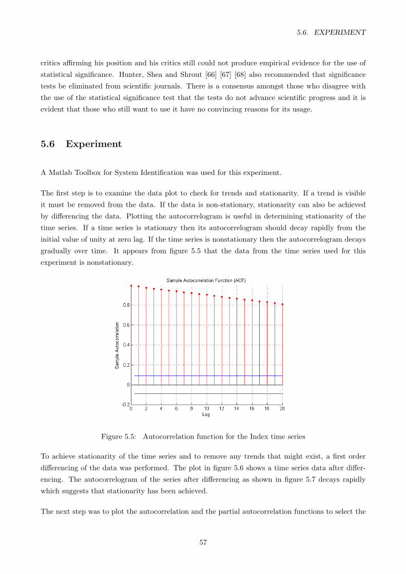
5.6. EXPERIMENT
critics affirming his position and his critics still could not produce empirical evidence for the use of
statistical significance. Hunter, Shea and Shrout [66] [67] [68] also recommended that significance
tests be eliminated from scientific journals. There is a consensus amongst those who disagree with
the use of the statistical significance test that the tests do not advance scientific progress and it is
evident that those who still want to use it have no convincing reasons for its usage.
5.6 Experiment
A Matlab Toolbox for System Identification was used for this experiment.
The first step is to examine the data plot to check for trends and stationarity. If a trend is visible
it must be removed from the data. If the data is non-stationary, stationarity can also be achieved
by differencing the data. Plotting the autocorrelogram is useful in determining stationarity of the
time series. If a time series is stationary then its autocorrelogram should decay rapidly from the
initial value of unity at zero lag. If the time series is nonstationary then the autocorrelogram decays
gradually over time. It appears from figure 5.5 that the data from the time series used for this
experiment is nonstationary.
Figure 5.5: Autocorrelation function for the Index time series
To achieve stationarity of the time series and to remove any trends that might exist, a first order
differencing of the data was performed. The plot in figure 5.6 shows a time series data after differ-
encing. The autocorrelogram of the series after differencing as shown in figure 5.7 decays rapidly
which suggests that stationarity has been achieved.
The next step was to plot the autocorrelation and the partial autocorrelation functions to select the
57
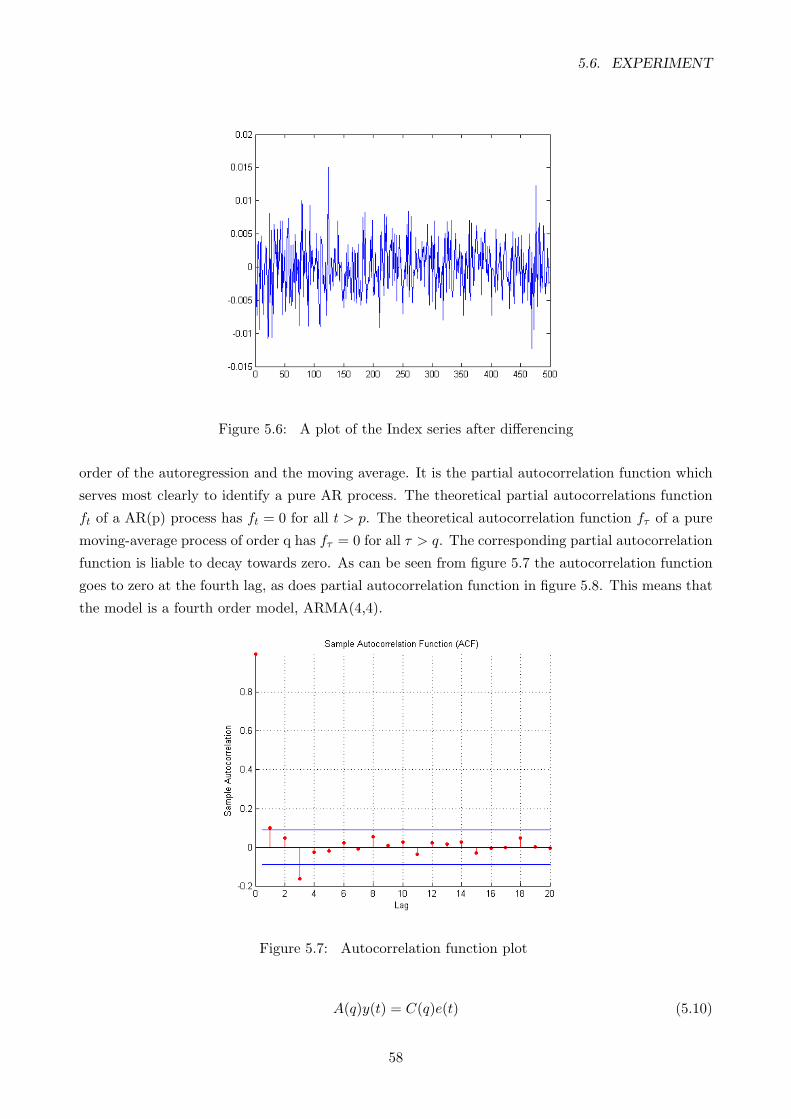
5.6. EXPERIMENT
Figure 5.6: A plot of the Index series after differencing
order of the autoregression and the moving average. It is the partial autocorrelation function which
serves most clearly to identify a pure AR process. The theoretical partial autocorrelations function
ft of a AR(p) process has ft = 0 for all t > p. The theoretical autocorrelation function fτ of a pure
moving-average process of order q has fτ = 0 for all τ > q. The corresponding partial autocorrelation
function is liable to decay towards zero. As can be seen from figure 5.7 the autocorrelation function
goes to zero at the fourth lag, as does partial autocorrelation function in figure 5.8. This means that
the model is a fourth order model, ARMA(4,4).
Figure 5.7: Autocorrelation function plot
A(q)y(t) = C(q)e(t) (5.10)
58
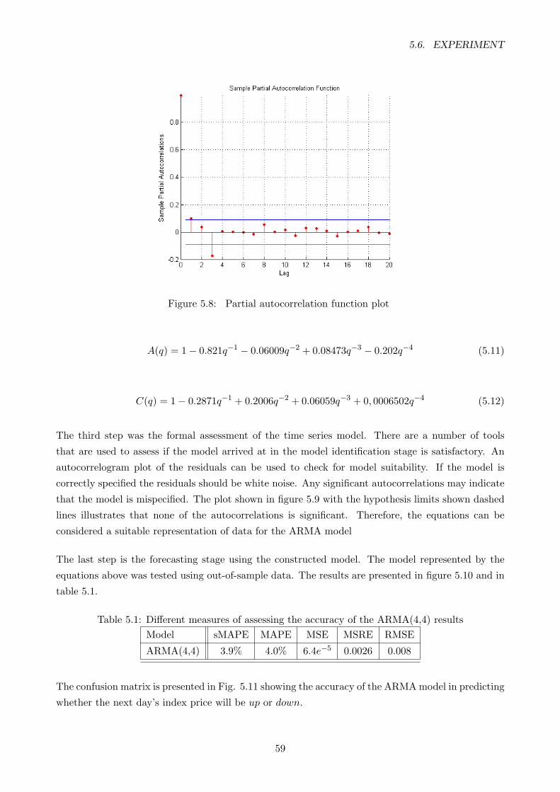
5.6. EXPERIMENT
Figure 5.8: Partial autocorrelation function plot
A(q) = 1− 0.821q−1 − 0.06009q−2 + 0.08473q−3 − 0.202q−4 (5.11)
C(q) = 1− 0.2871q−1 + 0.2006q−2 + 0.06059q−3 + 0, 0006502q−4 (5.12)
The third step was the formal assessment of the time series model. There are a number of tools
that are used to assess if the model arrived at in the model identification stage is satisfactory. An
autocorrelogram plot of the residuals can be used to check for model suitability. If the model is
correctly specified the residuals should be white noise. Any significant autocorrelations may indicate
that the model is mispecified. The plot shown in figure 5.9 with the hypothesis limits shown dashed
lines illustrates that none of the autocorrelations is significant. Therefore, the equations can be
considered a suitable representation of data for the ARMA model
The last step is the forecasting stage using the constructed model. The model represented by the
equations above was tested using out-of-sample data. The results are presented in figure 5.10 and in
table 5.1.
Table 5.1: Different measures of assessing the accuracy of the ARMA(4,4) resultsModel sMAPE MAPE MSE MSRE RMSE
ARMA(4,4) 3.9% 4.0% 6.4e−5 0.0026 0.008
The confusion matrix is presented in Fig. 5.11 showing the accuracy of the ARMA model in predicting
whether the next day’s index price will be up or down.
59
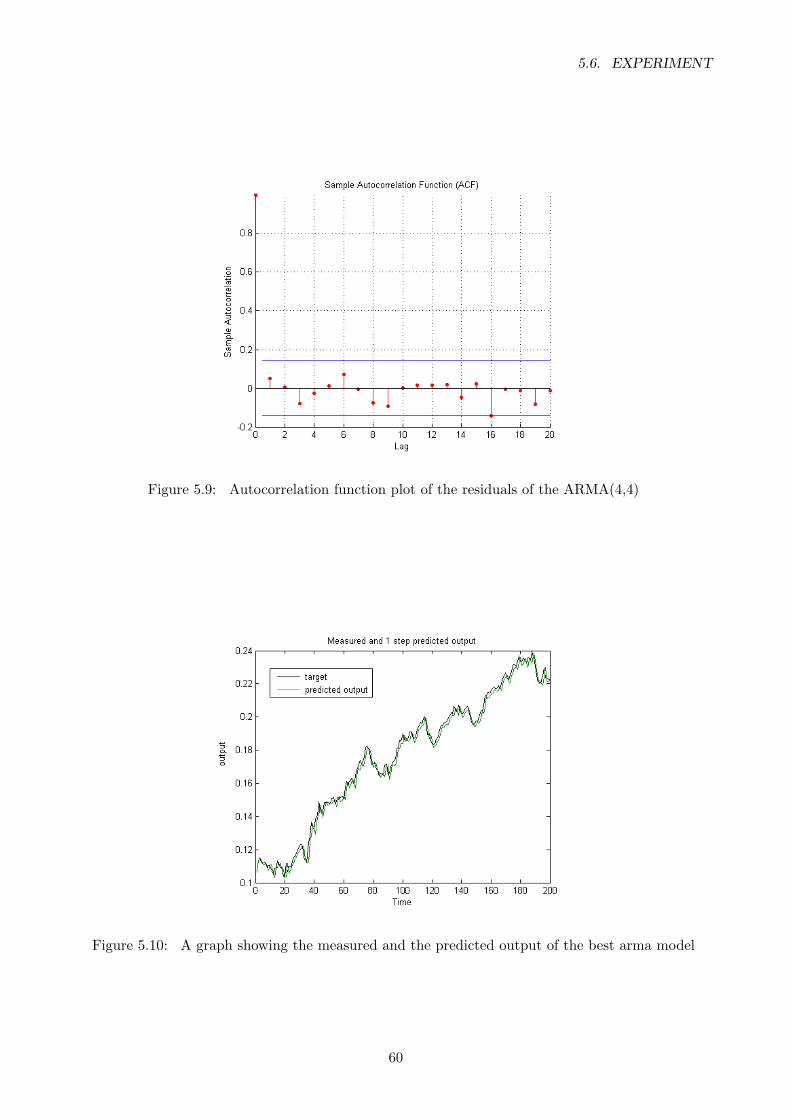
5.6. EXPERIMENT
Figure 5.9: Autocorrelation function plot of the residuals of the ARMA(4,4)
Figure 5.10: A graph showing the measured and the predicted output of the best arma model
60

5.6. EXPERIMENT
Figure 5.11: Confusion matrix for ARMA model prediction results.
Figure 5.12: Histogram of the ARMA prediction deviations
61
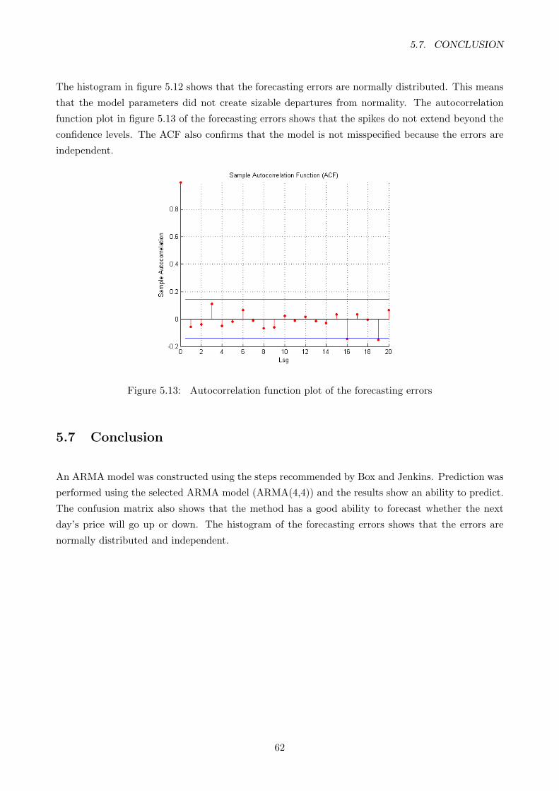
5.7. CONCLUSION
The histogram in figure 5.12 shows that the forecasting errors are normally distributed. This means
that the model parameters did not create sizable departures from normality. The autocorrelation
function plot in figure 5.13 of the forecasting errors shows that the spikes do not extend beyond the
confidence levels. The ACF also confirms that the model is not misspecified because the errors are
independent.
Figure 5.13: Autocorrelation function plot of the forecasting errors
5.7 Conclusion
An ARMA model was constructed using the steps recommended by Box and Jenkins. Prediction was
performed using the selected ARMA model (ARMA(4,4)) and the results show an ability to predict.
The confusion matrix also shows that the method has a good ability to forecast whether the next
day’s price will go up or down. The histogram of the forecasting errors shows that the errors are
normally distributed and independent.
62

Chapter 6
Prediction
6.1 Introduction
Finding a mathematical technique that has the ability to predict with good accuracy the future prices
of stocks is the subject of ongoing research. Investors are constantly trying to earn above average
returns from their investments on the stock market. Therefore, a model with the ability to predict
the stock price is of great interest to them. Various techniques have been used for this purpose,
some with success and others with failure. This work focused on building three computational
intelligence models. The chapter starts off with how the construction of the three models was done.
The chapter then focuses on the construction and testing of the models starting with multilayer
perceptron followed by support vector machines and lastly with neuro-fuzzy systems.
6.2 Model construction
After the data was preprocessed as described in chapter 5 in section 5.4 the next step was the creation
of the models. Window sizes of 3,5,7,10 were used for the extraction of the features that were used to
train and test the models. Figure 6.1 shows a flow diagram of how the models were created, trained
and tested.
6.3 Multilayer perceptron and ALSI prediction
Neural Networks have been applied to signal processing applications with great success. Financial
time series forecasting is an example of a signal processing problem which is characterised by non-
linearity and non-stationarity and therefore very complex to model. Using an advanced intelligent
63
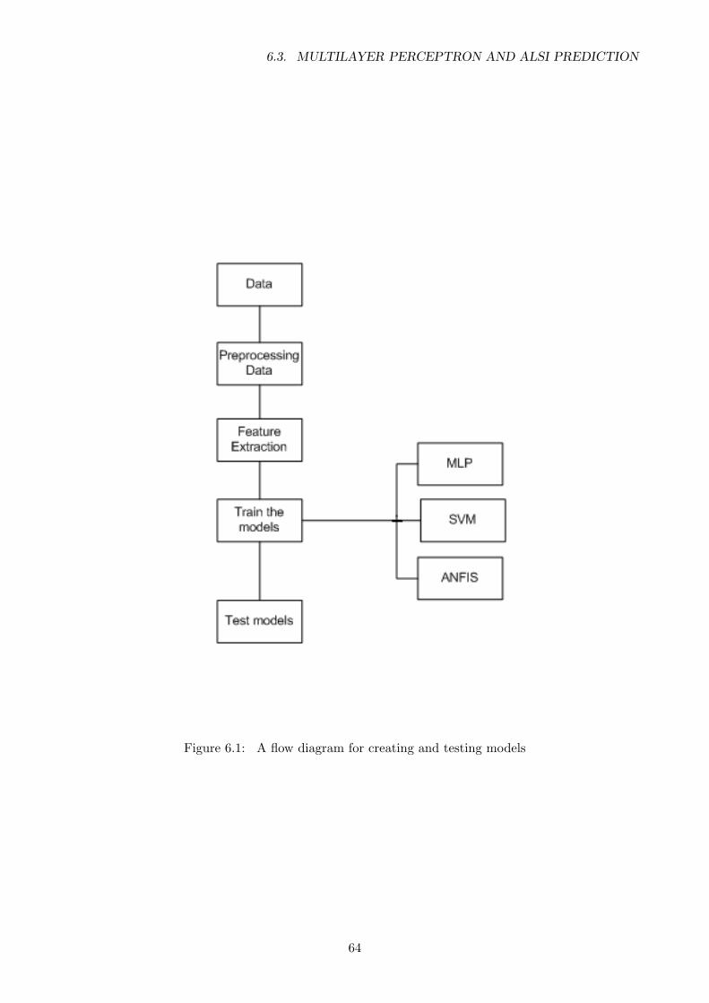
6.3. MULTILAYER PERCEPTRON AND ALSI PREDICTION
Figure 6.1: A flow diagram for creating and testing models
64
6.3. MULTILAYER PERCEPTRON AND ALSI PREDICTION
technique is regarded as an improvement from using traditional technical analysis techniques that
predicts stock prices based on historical prices and volume, basic concepts of trends, price patterns
and oscillators, commonly used by stock investors to aid investment decisions.
6.3.1 Multilayer perceptron
Multilayer perceptrons (MLPs) are feedforward neural networks trained with the standard backprop-
agation algorithm. This type of neural network falls under the supervised networks therefore they
require a desired output to be able to learn. They usually consists of three layers, the input layer,
hidden layer and the output layer. They have been shown to approximate the performance of optimal
statistical classifiers in difficult problems.
Multi layer perceptron architecture was chosen for the purpose of this experiment. The reason is
because MLP is the most common network architecture used for financial neural networks.
6.3.2 Learning environment
One of the most important steps of constructing a neural networks model is deciding on what infor-
mation to use to teach it. The main objective of forecasting with different tools is to decide when to
buy, hold or sell securities based on the information that is available about the security.
The input data may be raw data on volume, price, or daily change, but it may also include data
such as technical indicators (moving average, trend-line indicators, etc.) or fundamental indicators
(intrinsic share value, economic environment, etc.). One neural network system [13] used phrases
out of the president’s report to shareholders as input. These data may also include macroeconomic
indicators such as inflation, interest rate, gross domestic product (GDP), etc. For the purpose of this
project only the price of the all share index was available and was therefore used for the forecasting.
6.3.3 Network training
To train a neural network involves presenting it with different input patterns as contained in the data
so that the network can reduce its empirical error and improve its performance. The algorithm that
is used to train the network may vary depending on the network architecture, but the most common
training algorithm used when designing financial neural networks is the backpropagation algorithm.
Backpropagation is the process of backpropagating errors through the network from the output layer
towards the input layer during training. Backpropagation is necessary because hidden units have no
training target value that can be used, so they must be trained based on errors from previous layers.
65
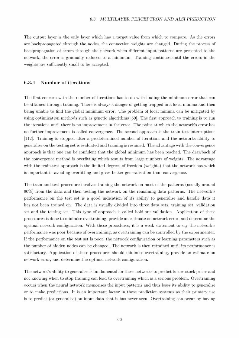
6.3. MULTILAYER PERCEPTRON AND ALSI PREDICTION
The output layer is the only layer which has a target value from which to compare. As the errors
are backpropagated through the nodes, the connection weights are changed. During the process of
backpropagation of errors through the network when different input patterns are presented to the
network, the error is gradually reduced to a minimum. Training continues until the errors in the
weights are sufficiently small to be accepted.
6.3.4 Number of iterations
The first concern with the number of iterations has to do with finding the minimum error that can
be attained through training. There is always a danger of getting trapped in a local minima and then
being unable to find the global minimum error. The problem of local minima can be mitigated by
using optimization methods such as genetic algorithms [69]. The first approach to training is to run
the iterations until there is no improvement in the error. The point at which the network’s error has
no further improvement is called convergence. The second approach is the train-test interruptions
[112]. Training is stopped after a predetermined number of iterations and the networks ability to
generalise on the testing set is evaluated and training is resumed. The advantage with the convergence
approach is that one can be confident that the global minimum has been reached. The drawback of
the convergence method is overfitting which results from large numbers of weights. The advantage
with the train-test approach is the limited degrees of freedom (weights) that the network has which
is important in avoiding overfitting and gives better generalisation than convergence.
The train and test procedure involves training the network on most of the patterns (usually around
90%) from the data and then testing the network on the remaining data patterns. The network’s
performance on the test set is a good indication of its ability to generalise and handle data it
has not been trained on. The data is usually divided into three data sets, training set, validation
set and the testing set. This type of approach is called hold-out validation. Application of these
procedures is done to minimise overtraining, provide an estimate on network error, and determine the
optimal network configuration. With these procedures, it is a weak statement to say the network’s
performance was poor because of overtraining, as overtraining can be controlled by the experimenter.
If the performance on the test set is poor, the network configuration or learning parameters such as
the number of hidden nodes can be changed. The network is then retrained until its performance is
satisfactory. Application of these procedures should minimise overtraining, provide an estimate on
network error, and determine the optimal network configuration.
The network’s ability to generalise is fundamental for these networks to predict future stock prices and
not knowing when to stop training can lead to overtraining which is a serious problem. Overtraining
occurs when the neural network memorises the input patterns and thus loses its ability to generalise
or to make predictions. It is an important factor in these prediction systems as their primary use
is to predict (or generalise) on input data that it has never seen. Overtraining can occur by having
66
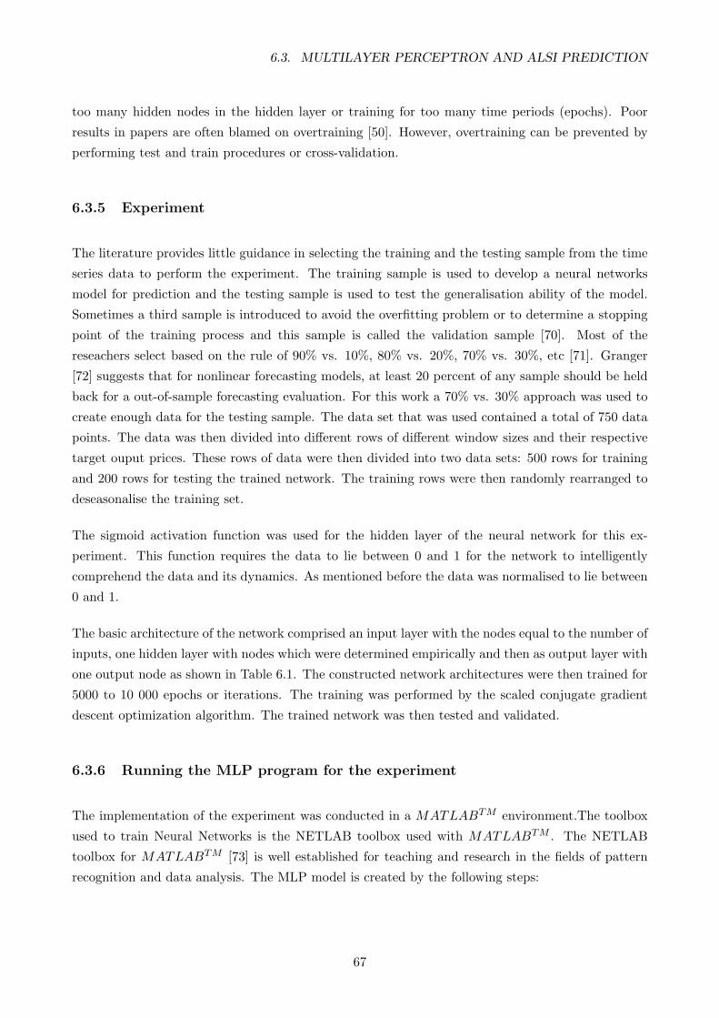
6.3. MULTILAYER PERCEPTRON AND ALSI PREDICTION
too many hidden nodes in the hidden layer or training for too many time periods (epochs). Poor
results in papers are often blamed on overtraining [50]. However, overtraining can be prevented by
performing test and train procedures or cross-validation.
6.3.5 Experiment
The literature provides little guidance in selecting the training and the testing sample from the time
series data to perform the experiment. The training sample is used to develop a neural networks
model for prediction and the testing sample is used to test the generalisation ability of the model.
Sometimes a third sample is introduced to avoid the overfitting problem or to determine a stopping
point of the training process and this sample is called the validation sample [70]. Most of the
reseachers select based on the rule of 90% vs. 10%, 80% vs. 20%, 70% vs. 30%, etc [71]. Granger
[72] suggests that for nonlinear forecasting models, at least 20 percent of any sample should be held
back for a out-of-sample forecasting evaluation. For this work a 70% vs. 30% approach was used to
create enough data for the testing sample. The data set that was used contained a total of 750 data
points. The data was then divided into different rows of different window sizes and their respective
target ouput prices. These rows of data were then divided into two data sets: 500 rows for training
and 200 rows for testing the trained network. The training rows were then randomly rearranged to
deseasonalise the training set.
The sigmoid activation function was used for the hidden layer of the neural network for this ex-
periment. This function requires the data to lie between 0 and 1 for the network to intelligently
comprehend the data and its dynamics. As mentioned before the data was normalised to lie between
0 and 1.
The basic architecture of the network comprised an input layer with the nodes equal to the number of
inputs, one hidden layer with nodes which were determined empirically and then as output layer with
one output node as shown in Table 6.1. The constructed network architectures were then trained for
5000 to 10 000 epochs or iterations. The training was performed by the scaled conjugate gradient
descent optimization algorithm. The trained network was then tested and validated.
6.3.6 Running the MLP program for the experiment
The implementation of the experiment was conducted in a MATLABTM environment.The toolbox
used to train Neural Networks is the NETLAB toolbox used with MATLABTM . The NETLAB
toolbox for MATLABTM [73] is well established for teaching and research in the fields of pattern
recognition and data analysis. The MLP model is created by the following steps:
67

6.3. MULTILAYER PERCEPTRON AND ALSI PREDICTION
Creating a network
For the matlab code that was used for this part of the experiment refer to appendix D (Appendix
D.3)
1. Select the number of inputs
2. Select the number of hidden nodes
3. Select the activation function
Training the network
1. Select the optimisation algorithm
2. Input the training and target data
3. Choose the number of epochs for training
4. Train the network
Testing the network
The trained network generalisation ability is then evaluated by testing the model using the testing
data set.
6.3.7 Results
Different architectures were used for this experiment. The results of the experiment are presented
in a graphical form and also in a table that compares the prediction accuracies of the different
architectures. Table 6.1 shows the different architectures that were constructed for the experiment.
The number of hidden nodes for the different models were determined empirically by testing different
networks with nodes from 2 to 30 nodes.
From Table 6.2 the accuracy of the model constructed with 5 inputs is more than all the other three
models. The model constructed with 10 inputs is much less accurate than all the other models, its
deviation is high. The reason for the poor performance of this model could be as a result of the
inability to capture the dynamics of the data. Overall the results show that MLP has the ability to
learn the non-linear relationships that exist between the input and the output. Graphs in Fig. 6.2 -
6.5 show that MLP is able to follow the trend of the target prices.
68
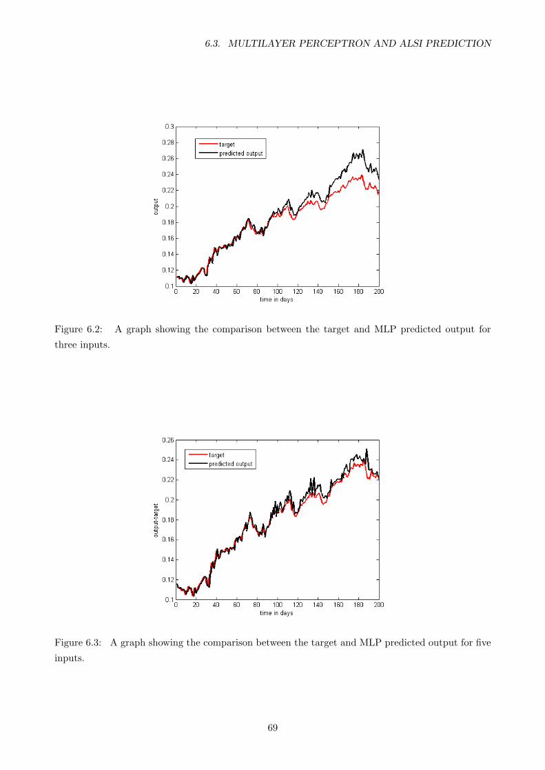
6.3. MULTILAYER PERCEPTRON AND ALSI PREDICTION
Figure 6.2: A graph showing the comparison between the target and MLP predicted output for
three inputs.
Figure 6.3: A graph showing the comparison between the target and MLP predicted output for five
inputs.
69
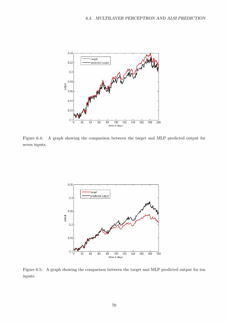
6.3. MULTILAYER PERCEPTRON AND ALSI PREDICTION
Figure 6.4: A graph showing the comparison between the target and MLP predicted output for
seven inputs.
Figure 6.5: A graph showing the comparison between the target and MLP predicted output for ten
inputs.
70
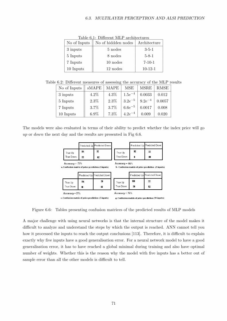
6.3. MULTILAYER PERCEPTRON AND ALSI PREDICTION
Table 6.1: Different MLP architecturesNo of Inputs No of hiddden nodes Architecture
3 inputs 5 nodes 3-5-1
5 Inputs 8 nodes 5-8-1
7 Inputs 10 nodes 7-10-1
10 Inputs 12 nodes 10-12-1
Table 6.2: Different measures of assessing the accuracy of the MLP resultsNo of Inputs sMAPE MAPE MSE MSRE RMSE
3 inputs 4.2% 4.3% 1.5e−4 0.0033 0.012
5 Inputs 2.3% 2.3% 3.2e−5 9.2e−4 0.0057
7 Inputs 3.7% 3.7% 6.6e−5 0.0017 0.008
10 Inputs 6.9% 7.3% 4.2e−4 0.009 0.020
The models were also evaluated in terms of their ability to predict whether the index price will go
up or down the next day and the results are presented in Fig 6.6.
Figure 6.6: Tables presenting confusion matrices of the predicted results of MLP models
A major challenge with using neural networks is that the internal structure of the model makes it
difficult to analyze and understand the steps by which the output is reached. ANN cannot tell you
how it processed the inputs to reach the output conclusions [113]. Therefore, it is difficult to explain
exactly why five inputs have a good generalisation error. For a neural network model to have a good
generalisation error, it has to have reached a global minimal during training and also have optimal
number of weights. Whether this is the reason why the model with five inputs has a better out of
sample error than all the other models is difficult to tell.
71
6.4. SUPPORT VECTOR REGRESSION AND ALSI FORECASTING
6.4 Support vector regression and ALSI forecasting
Since the creation of the SVM theory in 1995 by V. Vapnik, major breakthroughs have been recorded
in the application of SVM to time series forecasting. Most of the work that has been done in this
area has focused mainly on the ability of SVM to perform classification in research fields such as
documents classification, pattern recognition and also financial market prediction. The application of
support vector regressions (SVR) to financial market forecasting, estimation of power consumption
and reconstruction of chaotic systems is still under development. The great successes that SVM has
had in classification encourage research in using the SVR tool for the forecasting of the all share
index.
6.4.1 Support Vector Regression
The challenge of the regression problem is to determine a function that can accurately approximate
future values.
The Lagrange multipliers, α and α∗ represent solutions to the quadratic problem described in chapter
4 that act as forces pushing predictions towards the target value. Only the non-zero values of the
Lagrange multipliers in equation 4.31 (refer to chapter 4)are useful in forecasting the regression line
and are known as support vectors. For all points inside the ε -tube, the Lagrange multipliers equal
to zero do not contribute to the regression function.
The constant C introduced in equation 4.27 (refer to chapter 4) determines penalties to estimation
errors. A large C allocates higher penalties to errors so that the regression is trained to minimise
error with lower generalisation while a small C allocates fewer penalties to errors; this allows the
minimization of margin with errors, thus the model will have a higher generalisation ability. If C goes
to infinitely large, SVR would not allow the occurrence of any error and result in a complex model,
whereas when C goes to zero, the result would tolerate a large amount of errors and the model would
be less complex.
6.4.2 Experiment
There are three methods for controlling the regression model, the loss function, the kernel, and
additional capacity control. The experiments for the regression model used for the prediction of the
stock market index were performed with different ε -insensitive loss functions, with different kernels
and different degrees of capacity control. Several combinations were tried, and finally a radial basis
function was chosen as the kernel with ε = 0.01 and C = 100. The model is trained with the training
data set with 500 instances, and then tested with the test data set with another 200 instances.
72
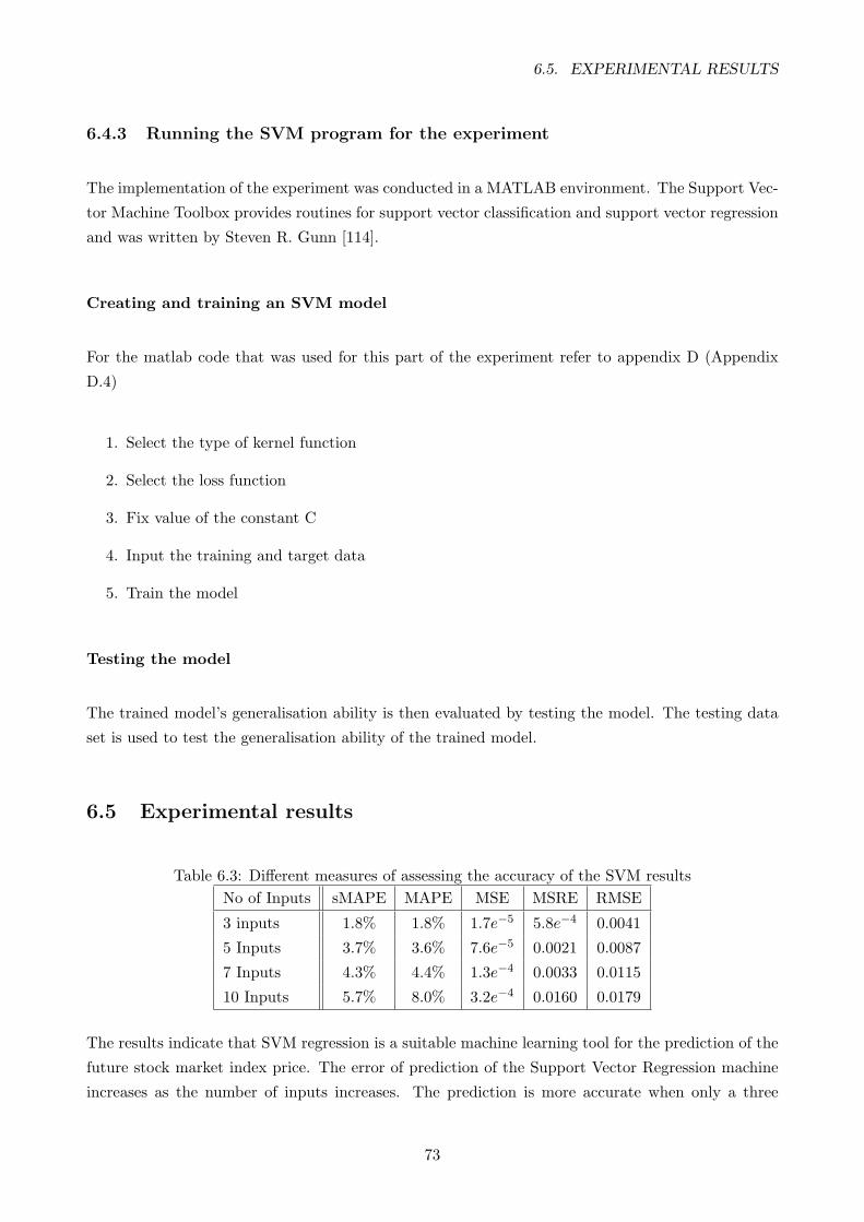
6.5. EXPERIMENTAL RESULTS
6.4.3 Running the SVM program for the experiment
The implementation of the experiment was conducted in a MATLAB environment. The Support Vec-
tor Machine Toolbox provides routines for support vector classification and support vector regression
and was written by Steven R. Gunn [114].
Creating and training an SVM model
For the matlab code that was used for this part of the experiment refer to appendix D (Appendix
D.4)
1. Select the type of kernel function
2. Select the loss function
3. Fix value of the constant C
4. Input the training and target data
5. Train the model
Testing the model
The trained model’s generalisation ability is then evaluated by testing the model. The testing data
set is used to test the generalisation ability of the trained model.
6.5 Experimental results
Table 6.3: Different measures of assessing the accuracy of the SVM resultsNo of Inputs sMAPE MAPE MSE MSRE RMSE
3 inputs 1.8% 1.8% 1.7e−5 5.8e−4 0.0041
5 Inputs 3.7% 3.6% 7.6e−5 0.0021 0.0087
7 Inputs 4.3% 4.4% 1.3e−4 0.0033 0.0115
10 Inputs 5.7% 8.0% 3.2e−4 0.0160 0.0179
The results indicate that SVM regression is a suitable machine learning tool for the prediction of the
future stock market index price. The error of prediction of the Support Vector Regression machine
increases as the number of inputs increases. The prediction is more accurate when only a three
73
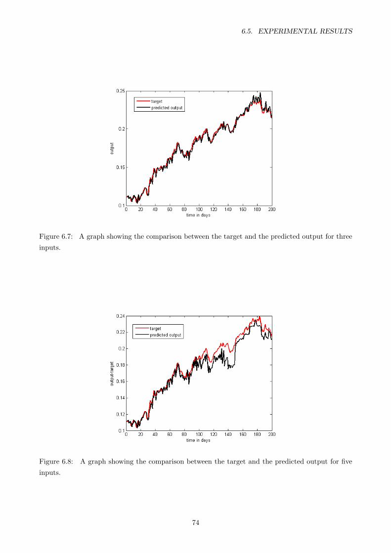
6.5. EXPERIMENTAL RESULTS
Figure 6.7: A graph showing the comparison between the target and the predicted output for three
inputs.
Figure 6.8: A graph showing the comparison between the target and the predicted output for five
inputs.
74
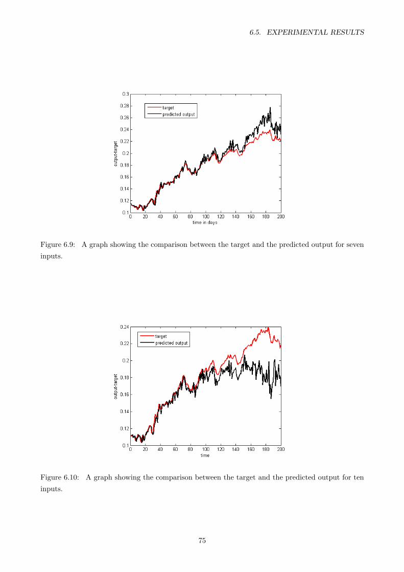
6.5. EXPERIMENTAL RESULTS
Figure 6.9: A graph showing the comparison between the target and the predicted output for seven
inputs.
Figure 6.10: A graph showing the comparison between the target and the predicted output for ten
inputs.
75
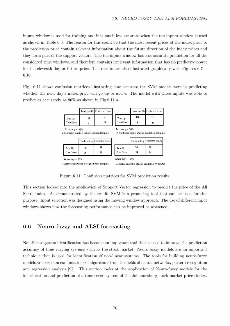
6.6. NEURO-FUZZY AND ALSI FORECASTING
inputs window is used for training and it is much less accurate when the ten inputs window is used
as shown in Table 6.3. The reason for this could be that the most recent prices of the index prior to
the prediction price contain relevant information about the future direction of the index prices and
they form part of the support vectors. The ten inputs window has less accurate prediction for all the
considered time windows, and therefore contains irrelevant information that has no predictive power
for the eleventh day or future price. The results are also illustrated graphically with Figures 6.7 -
6.10.
Fig. 6.11 shows confusion matrices illustrating how accurate the SVM models were in predicting
whether the next day’s index price will go up or down. The model with three inputs was able to
predict as accurately as 96% as shown in Fig.6.11 a.
Figure 6.11: Confusion matrices for SVM prediction results.
This section looked into the application of Support Vector regression to predict the price of the All
Share Index. As demonstrated by the results SVM is a promising tool that can be used for this
purpose. Input selection was designed using the moving window approach. The use of different input
windows shows how the forecasting performance can be improved or worsened.
6.6 Neuro-fuzzy and ALSI forecasting
Non-linear system identification has become an important tool that is used to improve the prediction
accuracy of time varying systems such as the stock market. Neuro-fuzzy models are an important
technique that is used for identification of non-linear systems. The tools for building neuro-fuzzy
models are based on combinations of algorithms from the fields of neural networks, pattern recognition
and regression analysis [97]. This section looks at the application of Neuro-fuzzy models for the
identification and prediction of a time series system of the Johannesburg stock market prices index.
76
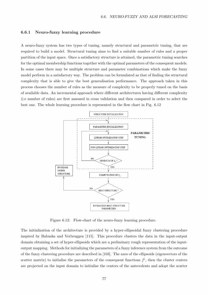
6.6. NEURO-FUZZY AND ALSI FORECASTING
6.6.1 Neuro-fuzzy learning procedure
A neuro-fuzzy system has two types of tuning, namely structural and parametric tuning, that are
required to build a model. Structural tuning aims to find a suitable number of rules and a proper
partition of the input space. Once a satisfactory structure is attained, the parametric tuning searches
for the optimal membership functions together with the optimal parameters of the consequent models.
In some cases there may be multiple structure and parameter combinations which make the fuzzy
model perform in a satisfactory way. The problem can be formulated as that of finding the structural
complexity that is able to give the best generalisation performance. The approach taken in this
process chooses the number of rules as the measure of complexity to be properly tuned on the basis
of available data. An incremental approach where different architectures having different complexity
(i.e number of rules) are first assessed in cross validation and then compared in order to select the
best one. The whole learning procedure is represented in the flow chart in Fig. 6.12
Figure 6.12: Flow-chart of the neuro-fuzzy learning procedure.
The initialization of the architecture is provided by a hyper-ellipsoidal fuzzy clustering procedure
inspired by Babuska and Verbruggen [115]. This procedure clusters the data in the input-output
domain obtaining a set of hyper-ellipsoids which are a preliminary rough representation of the input-
output mapping. Methods for initializing the parameters of a fuzzy inference system from the outcome
of the fuzzy clustering procedure are described in [103]. The axes of the ellipsoids (eigenvectors of the
scatter matrix) to initialise the parameters of the consequent functions f i, then the cluster centers
are projected on the input domain to initialise the centers of the antecedents and adopt the scatter
77
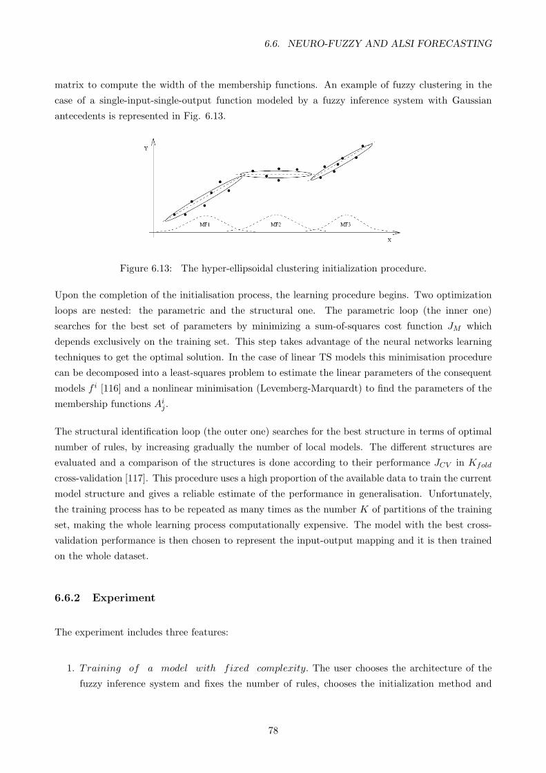
6.6. NEURO-FUZZY AND ALSI FORECASTING
matrix to compute the width of the membership functions. An example of fuzzy clustering in the
case of a single-input-single-output function modeled by a fuzzy inference system with Gaussian
antecedents is represented in Fig. 6.13.
Figure 6.13: The hyper-ellipsoidal clustering initialization procedure.
Upon the completion of the initialisation process, the learning procedure begins. Two optimization
loops are nested: the parametric and the structural one. The parametric loop (the inner one)
searches for the best set of parameters by minimizing a sum-of-squares cost function JM which
depends exclusively on the training set. This step takes advantage of the neural networks learning
techniques to get the optimal solution. In the case of linear TS models this minimisation procedure
can be decomposed into a least-squares problem to estimate the linear parameters of the consequent
models f i [116] and a nonlinear minimisation (Levemberg-Marquardt) to find the parameters of the
membership functions Aij .
The structural identification loop (the outer one) searches for the best structure in terms of optimal
number of rules, by increasing gradually the number of local models. The different structures are
evaluated and a comparison of the structures is done according to their performance JCV in Kfold
cross-validation [117]. This procedure uses a high proportion of the available data to train the current
model structure and gives a reliable estimate of the performance in generalisation. Unfortunately,
the training process has to be repeated as many times as the number K of partitions of the training
set, making the whole learning process computationally expensive. The model with the best cross-
validation performance is then chosen to represent the input-output mapping and it is then trained
on the whole dataset.
6.6.2 Experiment
The experiment includes three features:
1. Training of a model with fixed complexity. The user chooses the architecture of the
fuzzy inference system and fixes the number of rules, chooses the initialization method and
78
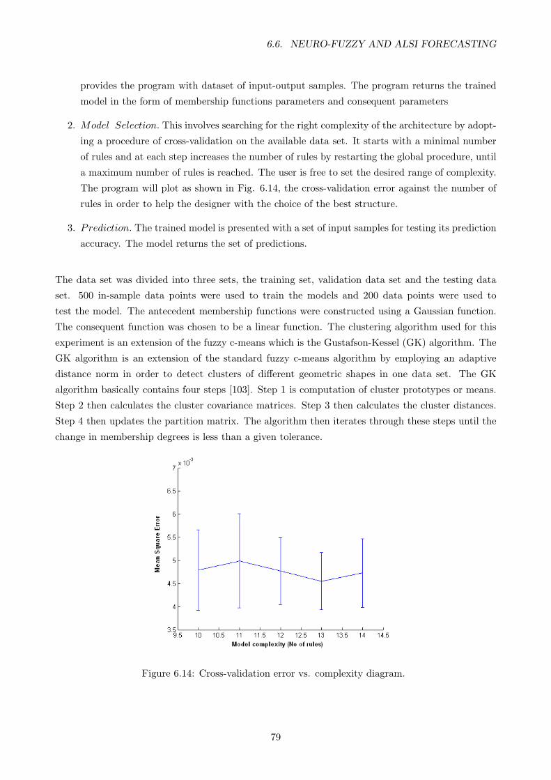
6.6. NEURO-FUZZY AND ALSI FORECASTING
provides the program with dataset of input-output samples. The program returns the trained
model in the form of membership functions parameters and consequent parameters
2. Model Selection. This involves searching for the right complexity of the architecture by adopt-
ing a procedure of cross-validation on the available data set. It starts with a minimal number
of rules and at each step increases the number of rules by restarting the global procedure, until
a maximum number of rules is reached. The user is free to set the desired range of complexity.
The program will plot as shown in Fig. 6.14, the cross-validation error against the number of
rules in order to help the designer with the choice of the best structure.
3. Prediction. The trained model is presented with a set of input samples for testing its prediction
accuracy. The model returns the set of predictions.
The data set was divided into three sets, the training set, validation data set and the testing data
set. 500 in-sample data points were used to train the models and 200 data points were used to
test the model. The antecedent membership functions were constructed using a Gaussian function.
The consequent function was chosen to be a linear function. The clustering algorithm used for this
experiment is an extension of the fuzzy c-means which is the Gustafson-Kessel (GK) algorithm. The
GK algorithm is an extension of the standard fuzzy c-means algorithm by employing an adaptive
distance norm in order to detect clusters of different geometric shapes in one data set. The GK
algorithm basically contains four steps [103]. Step 1 is computation of cluster prototypes or means.
Step 2 then calculates the cluster covariance matrices. Step 3 then calculates the cluster distances.
Step 4 then updates the partition matrix. The algorithm then iterates through these steps until the
change in membership degrees is less than a given tolerance.
Figure 6.14: Cross-validation error vs. complexity diagram.
79

6.6. NEURO-FUZZY AND ALSI FORECASTING
6.6.3 Running the program for the experiment
Searching for model complexity
The first step of running the neuro-fuzzy programmme is for searching the model complexity. MAT-
LAB software tool for neuro-fuzzy identification and data analysis. Ver. 0.1 was used written by
Gianluca Bontempi and Mauro Bitattari [118].
For the matlab code that was used for this part of the experiment refer to appendix D (Appendix
D.5)
1. Select the type of membership function
2. Select the type clustering technique e.g. Hard fuzzy c-means
3. Select the form of the consequent model e.g. Linear or Constant
4. Indicate the minimum number of rules
5. Indicate the maximum number of rules
6. Select the number of cross validation sets
7. Get training and target inputs
8. Run the programme to get the model
The data in this step is partitioned into clusters of the chosen membership function. The clusters
vary in sizes. From these clusters a number of fuzzy rules are extracted and defined as explained in
chapter 4.
Training the model of a fixed complexity
To train the model, the train and target inputs from the data set used to search for the model
complexity is used to train the model. The trained model is then saved to be evaluated. The
training is similar to the MLP training in that the gradient descent method of finding the minimum
error is used.
Testing the trained model
The testing set of the data is then used to evaluate the predictive power of the model. The error is
also evaluated using various error measures.
80
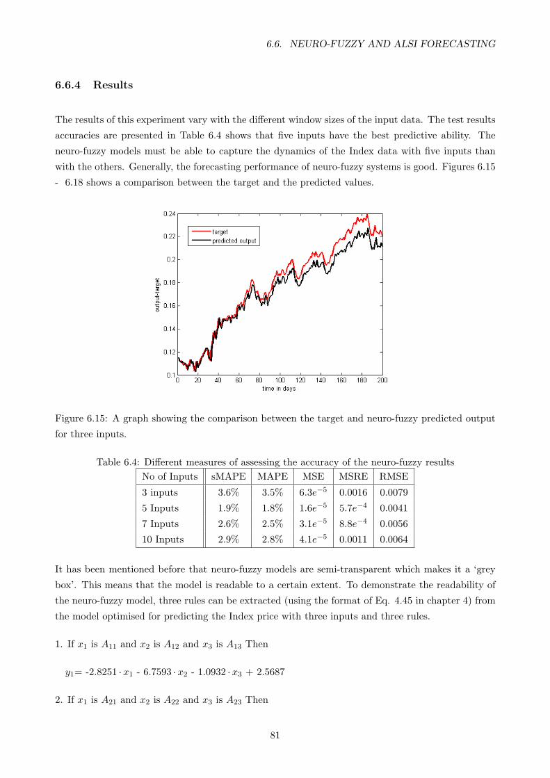
6.6. NEURO-FUZZY AND ALSI FORECASTING
6.6.4 Results
The results of this experiment vary with the different window sizes of the input data. The test results
accuracies are presented in Table 6.4 shows that five inputs have the best predictive ability. The
neuro-fuzzy models must be able to capture the dynamics of the Index data with five inputs than
with the others. Generally, the forecasting performance of neuro-fuzzy systems is good. Figures 6.15
- 6.18 shows a comparison between the target and the predicted values.
Figure 6.15: A graph showing the comparison between the target and neuro-fuzzy predicted output
for three inputs.
Table 6.4: Different measures of assessing the accuracy of the neuro-fuzzy resultsNo of Inputs sMAPE MAPE MSE MSRE RMSE
3 inputs 3.6% 3.5% 6.3e−5 0.0016 0.0079
5 Inputs 1.9% 1.8% 1.6e−5 5.7e−4 0.0041
7 Inputs 2.6% 2.5% 3.1e−5 8.8e−4 0.0056
10 Inputs 2.9% 2.8% 4.1e−5 0.0011 0.0064
It has been mentioned before that neuro-fuzzy models are semi-transparent which makes it a ‘grey
box’. This means that the model is readable to a certain extent. To demonstrate the readability of
the neuro-fuzzy model, three rules can be extracted (using the format of Eq. 4.45 in chapter 4) from
the model optimised for predicting the Index price with three inputs and three rules.
1. If x1 is A11 and x2 is A12 and x3 is A13 Then
y1= -2.8251 ·x1 - 6.7593 ·x2 - 1.0932 ·x3 + 2.5687
2. If x1 is A21 and x2 is A22 and x3 is A23 Then
81
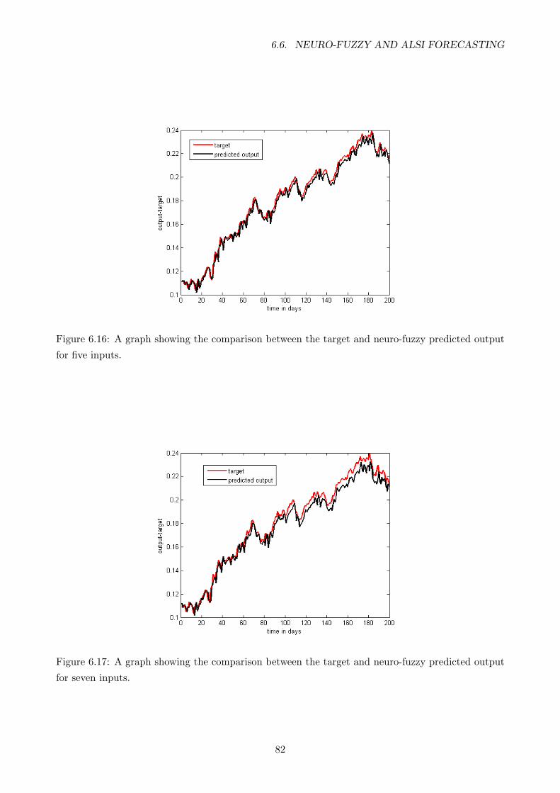
6.6. NEURO-FUZZY AND ALSI FORECASTING
Figure 6.16: A graph showing the comparison between the target and neuro-fuzzy predicted output
for five inputs.
Figure 6.17: A graph showing the comparison between the target and neuro-fuzzy predicted output
for seven inputs.
82
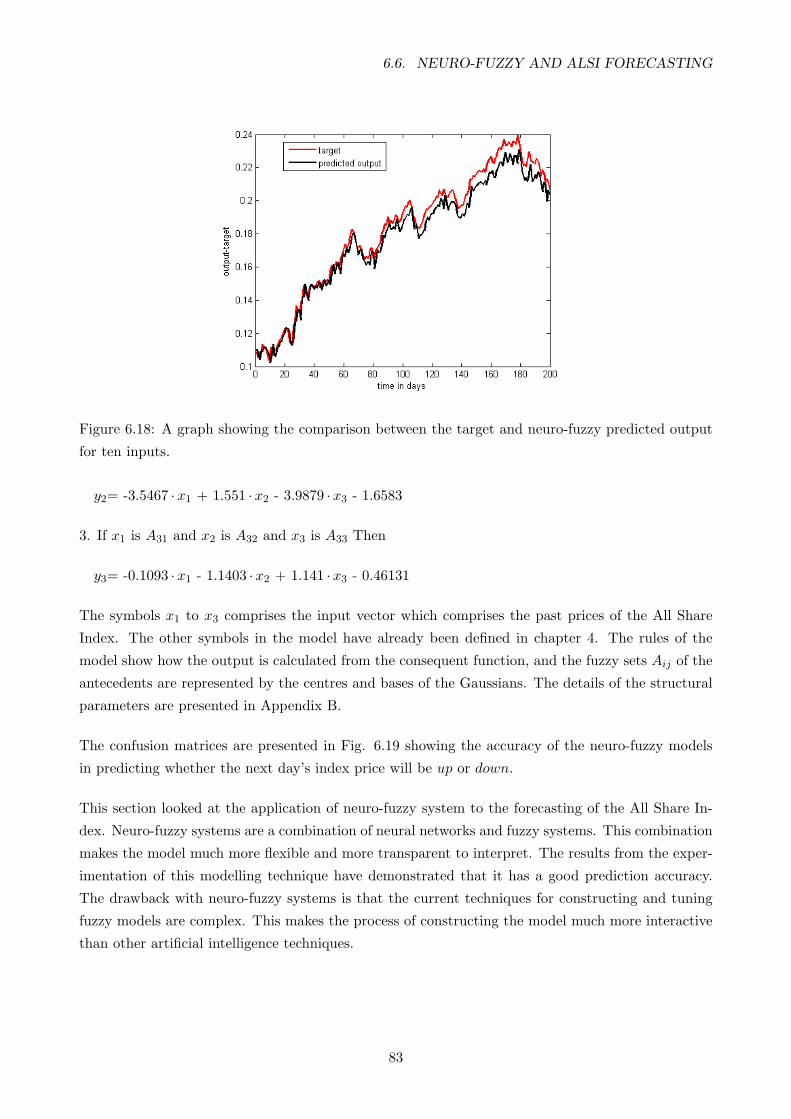
6.6. NEURO-FUZZY AND ALSI FORECASTING
Figure 6.18: A graph showing the comparison between the target and neuro-fuzzy predicted output
for ten inputs.
y2= -3.5467 ·x1 + 1.551 ·x2 - 3.9879 ·x3 - 1.6583
3. If x1 is A31 and x2 is A32 and x3 is A33 Then
y3= -0.1093 ·x1 - 1.1403 ·x2 + 1.141 ·x3 - 0.46131
The symbols x1 to x3 comprises the input vector which comprises the past prices of the All Share
Index. The other symbols in the model have already been defined in chapter 4. The rules of the
model show how the output is calculated from the consequent function, and the fuzzy sets Aij of the
antecedents are represented by the centres and bases of the Gaussians. The details of the structural
parameters are presented in Appendix B.
The confusion matrices are presented in Fig. 6.19 showing the accuracy of the neuro-fuzzy models
in predicting whether the next day’s index price will be up or down.
This section looked at the application of neuro-fuzzy system to the forecasting of the All Share In-
dex. Neuro-fuzzy systems are a combination of neural networks and fuzzy systems. This combination
makes the model much more flexible and more transparent to interpret. The results from the exper-
imentation of this modelling technique have demonstrated that it has a good prediction accuracy.
The drawback with neuro-fuzzy systems is that the current techniques for constructing and tuning
fuzzy models are complex. This makes the process of constructing the model much more interactive
than other artificial intelligence techniques.
83
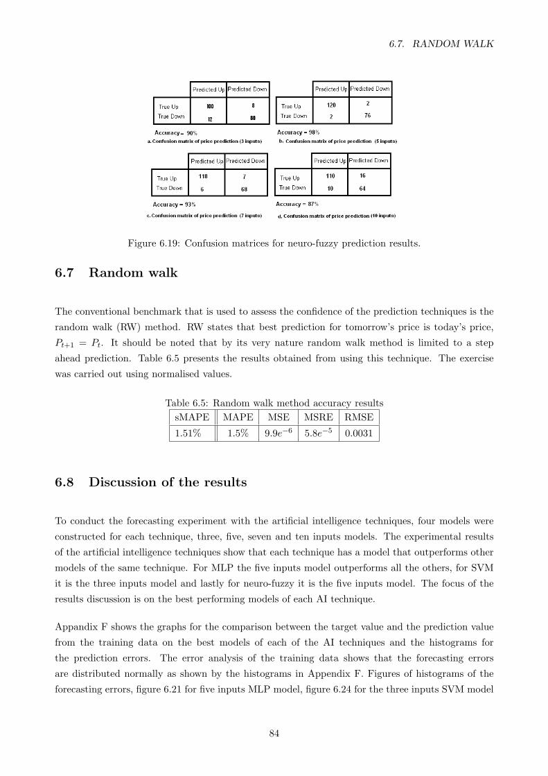
6.7. RANDOM WALK
Figure 6.19: Confusion matrices for neuro-fuzzy prediction results.
6.7 Random walk
The conventional benchmark that is used to assess the confidence of the prediction techniques is the
random walk (RW) method. RW states that best prediction for tomorrow’s price is today’s price,
Pt+1 = Pt. It should be noted that by its very nature random walk method is limited to a step
ahead prediction. Table 6.5 presents the results obtained from using this technique. The exercise
was carried out using normalised values.
Table 6.5: Random walk method accuracy resultssMAPE MAPE MSE MSRE RMSE
1.51% 1.5% 9.9e−6 5.8e−5 0.0031
6.8 Discussion of the results
To conduct the forecasting experiment with the artificial intelligence techniques, four models were
constructed for each technique, three, five, seven and ten inputs models. The experimental results
of the artificial intelligence techniques show that each technique has a model that outperforms other
models of the same technique. For MLP the five inputs model outperforms all the others, for SVM
it is the three inputs model and lastly for neuro-fuzzy it is the five inputs model. The focus of the
results discussion is on the best performing models of each AI technique.
Appandix F shows the graphs for the comparison between the target value and the prediction value
from the training data on the best models of each of the AI techniques and the histograms for
the prediction errors. The error analysis of the training data shows that the forecasting errors
are distributed normally as shown by the histograms in Appendix F. Figures of histograms of the
forecasting errors, figure 6.21 for five inputs MLP model, figure 6.24 for the three inputs SVM model
84
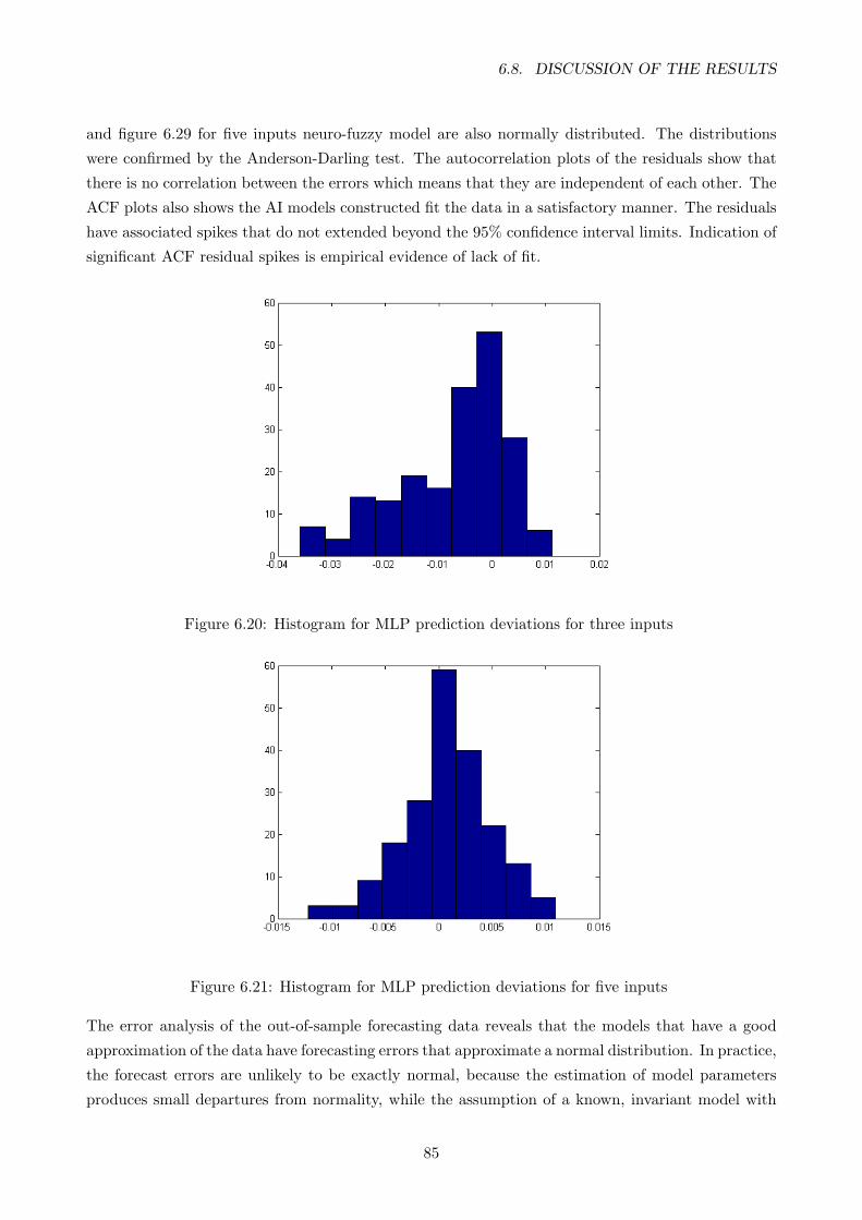
6.8. DISCUSSION OF THE RESULTS
and figure 6.29 for five inputs neuro-fuzzy model are also normally distributed. The distributions
were confirmed by the Anderson-Darling test. The autocorrelation plots of the residuals show that
there is no correlation between the errors which means that they are independent of each other. The
ACF plots also shows the AI models constructed fit the data in a satisfactory manner. The residuals
have associated spikes that do not extended beyond the 95% confidence interval limits. Indication of
significant ACF residual spikes is empirical evidence of lack of fit.
Figure 6.20: Histogram for MLP prediction deviations for three inputs
Figure 6.21: Histogram for MLP prediction deviations for five inputs
The error analysis of the out-of-sample forecasting data reveals that the models that have a good
approximation of the data have forecasting errors that approximate a normal distribution. In practice,
the forecast errors are unlikely to be exactly normal, because the estimation of model parameters
produces small departures from normality, while the assumption of a known, invariant model with
85
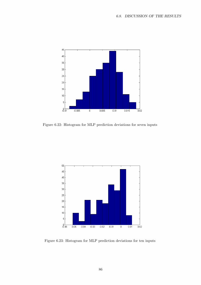
6.8. DISCUSSION OF THE RESULTS
Figure 6.22: Histogram for MLP prediction deviations for seven inputs
Figure 6.23: Histogram for MLP prediction deviations for ten inputs
86
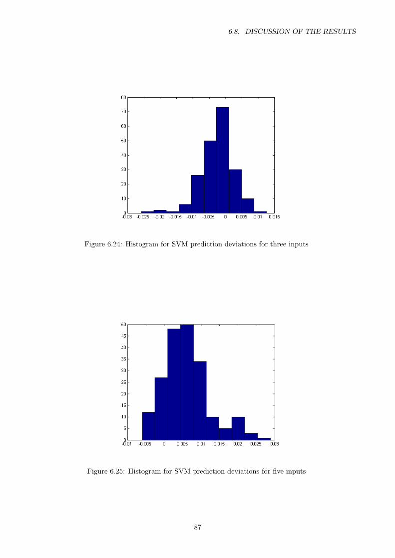
6.8. DISCUSSION OF THE RESULTS
Figure 6.24: Histogram for SVM prediction deviations for three inputs
Figure 6.25: Histogram for SVM prediction deviations for five inputs
87

6.8. DISCUSSION OF THE RESULTS
Figure 6.26: Histogram for SVM prediction deviations for seven inputs
Figure 6.27: Histogram for SVM prediction deviations for ten inputs
88
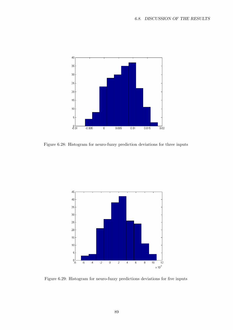
6.8. DISCUSSION OF THE RESULTS
Figure 6.28: Histogram for neuro-fuzzy prediction deviations for three inputs
Figure 6.29: Histogram for neuro-fuzzy predictions deviations for five inputs
89
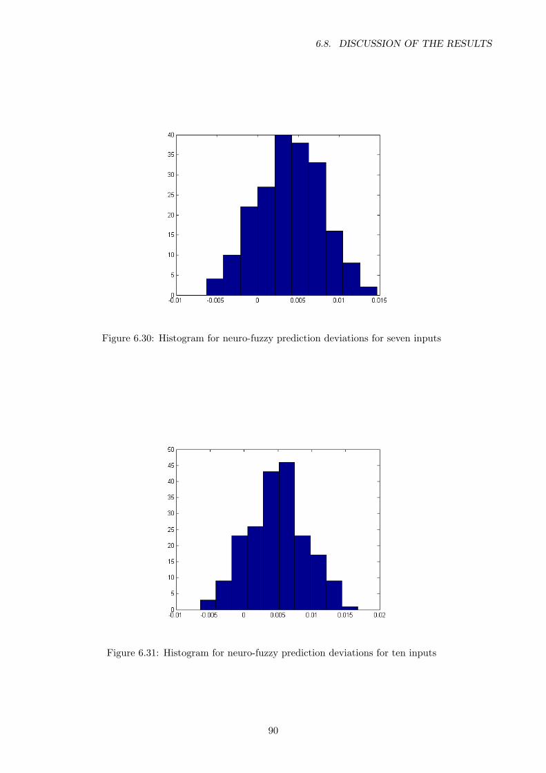
6.8. DISCUSSION OF THE RESULTS
Figure 6.30: Histogram for neuro-fuzzy prediction deviations for seven inputs
Figure 6.31: Histogram for neuro-fuzzy prediction deviations for ten inputs
90

6.8. DISCUSSION OF THE RESULTS
normal errors is also unlikely to be true [16]. Using the Anderson-Darling test the results of the
distribution of the forecasting are as follows:
MLP five inputs model forecasting errors:
1. Sample size: 200
2. Anderson-Darling statistic: 0.2045
3. Anderson-Darling adjusted statistic: 0.2053
4. Probability associated to the Anderson-Darling statistic = 0.8723
5. With a given significance = 0.050
6. The sampled population is normally distributed.
7. Thus, this sample has been drawn from a normal population with a mean and variance =
0.00280 0.0000
SVM three inputs model forecasting errors:
1. Sample size: 200
2. Anderson-Darling statistic: 0.4100
3. Anderson-Darling adjusted statistic: 0.4116
4. Probability associated to the Anderson-Darling statistic = 0.3406
5. With a given significance = 0.050
6. The sampled population is normally distributed.
7. Thus, this sample has been drawn from a normal population with a mean and variance = -
0.0048 0.0000
Neuro-fuzzy five inputs forecasting errors:
1. Sample size: 200
2. Anderson-Darling statistic: 0.1893
3. Anderson-Darling adjusted statistic: 0.1901
91
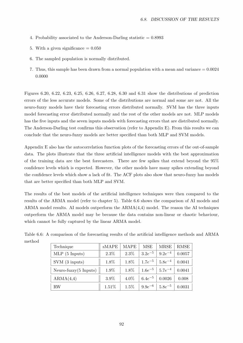
6.8. DISCUSSION OF THE RESULTS
4. Probability associated to the Anderson-Darling statistic = 0.8993
5. With a given significance = 0.050
6. The sampled population is normally distributed.
7. Thus, this sample has been drawn from a normal population with a mean and variance = 0.0024
0.0000
Figures 6.20, 6.22, 6.23, 6.25, 6.26, 6.27, 6.28, 6.30 and 6.31 show the distributions of prediction
errors of the less accurate models. Some of the distributions are normal and some are not. All the
neuro-fuzzy models have their forecasting errors distributed normally. SVM has the three inputs
model forecasting error distributed normally and the rest of the other models are not. MLP models
has the five inputs and the seven inputs models with forecasting errors that are distributed normally.
The Anderson-Darling test confirms this observation (refer to Appendix E). From this results we can
conclude that the neuro-fuzzy models are better specified than both MLP and SVM models.
Appendix E also has the autocorrelation function plots of the forecasting errors of the out-of-sample
data. The plots illustrate that the three artificial intelligence models with the best approximation
of the training data are the best forecasters. There are few spikes that extend beyond the 95%
confidence levels which is expected. However, the other models have many spikes extending beyond
the confidence levels which show a lack of fit. The ACF plots also show that neuro-fuzzy has models
that are better specified than both MLP and SVM.
The results of the best models of the artificial intelligence techniques were then compared to the
results of the ARMA model (refer to chapter 5). Table 6.6 shows the comparison of AI models and
ARMA model results. AI models outperform the ARMA(4,4) model. The reason the AI techniques
outperform the ARMA model may be because the data contains non-linear or chaotic behaviour,
which cannot be fully captured by the linear ARMA model.
Table 6.6: A comparison of the forecasting results of the artificial intelligence methods and ARMA
methodTechnique sMAPE MAPE MSE MRSE RMSE
MLP (5 Inputs) 2.3% 2.3% 3.2e−5 9.2e−4 0.0057
SVM (3 inputs) 1.8% 1.8% 1.7e−5 5.8e−4 0.0041
Neuro-fuzzy(5 Inputs) 1.9% 1.8% 1.6e−5 5.7e−4 0.0041
ARMA(4,4) 3.9% 4.0% 6.4e−5 0.0026 0.008
RW 1.51% 1.5% 9.9e−6 5.8e−5 0.0031
92

6.9. CONCLUSION
6.9 Conclusion
This chapter focused on the application of the three computational intelligence techniques to the fore-
casting of the JSE All Share Index. The results obtained from the testing of the models constructed
demonstrate that all three techniques have the ability to forecast the price of the index. A closer look
at the results reveals that the conclusion that the ranking of accuracy for different algorithms could
only be reached in cases where the performance of the algorithms compared has a small deviation.
For example, in comparing the accuracy of MLP versus neuro-fuzzy with the results from five inputs,
it was found that the ranking was very dependent on the accuracy measure used. However, another
finding with accuracy measures was that in cases where the deviation of the compared accuracies
was large, the ranking was independent of the accuracy measures. The example of this is striking
when comparing the accuracy of SVM versus MLP for three inputs predictions, the outperformance
of SVM over MLP is consistent across the various accuracy measures.
What is also very evident from the results is that MLP and neuro-fuzzy have both had their best
results at five inputs. Considering that both have similar learning algorithms, it is not surprising to
get this outcome. SVM had its best performance when the model was constructed with three inputs.
The results of the Artificial intelligence techniques were then compared to the benchmark model,
ARMA model, results and it was found that the AI models outperform the ARMA model. All the
Models were then compared to the naive random walk model and they were all outperformed.
93
Chapter 7
Conclusion
Three artificial intelligence techniques were applied to the prediction of the future price index of
the stock market. Artificial neural networks, support vector machines and neuro-fuzzy systems were
used to predict the JSE composite price index. The approach taken for this project was to predict
the future price of the All Share Index. The vast amount of work done in this area with all three
techniques has focused more on predicting the direction of the future price. This means that most
researchers just wanted to know whether the stock price will go up or down in the future. Determining
the direction does not reveal the margin of increase or decrease of the price. The results obtained
show that all three techniques have the ability to forecast the price of the index. Forecasting the
price is much more challenging than simply the direction. If it is predicted within a certain level
of accuracy it can provide more information about the future behaviour of the market stock price.
This sends a good message to investors that computational intelligence techniques can be used for
forecasting in the market. Another objective of the study was to demonstrate that the past prices
of stocks have predictive power. The results have shown that past stock prices contain information
that can be used to predict the future prices.
7.1 Transaction costs and EMH
The question that can be asked about the results presented in this research is: Do the results refute
Efficient Market Hypothesis? EMH is disproved when an investor consistently achieves above average
returns on the market. This would require the returns achieved to be higher than the transaction
costs. Returns depend on the magnitude of the price increase (to be predicted), the accuracy of the
prediction and number of shares (volume) to be traded. Using the prediction measurements from the
three techniques, there are instances where the returns yielded would be good and where it would
not. The answer to this question is not an easy one but the results have to some extent shown that
the market is not as efficient as EMH claims. Further studies will need to be conducted for a clear
conclusion to be made about the validity of EMH in the JSE.
94
7.2. COMPARISON OF THE TECHNIQUES
An analysis into whether the one step predictions conducted for this research will yield returns that
can overcome the transaction costs yields mixed results. Investors do not only incur costs that have
been mentioned, at times it is difficult to know what other costs are faced by investors. For example,
if an investor borrows money to invest in the stock market, the cost of such a loan maybe high or low
depending on his credit rating and that cost would play an important role in determining whether
he should invest or not. There are instances where the return would yield a good return and where it
would not. The models can yield an accurate prediction but that could be worthless to an investor if
the magnitude of the change from the previous day’s price is not large enough to warrant trading of
shares. Therefore, a conclusion as to whether the EMH is refuted when transaction costs are factored
in, cannot be made. For an investor to use these models profitably an individual’s discretion will
have to be exercised.
7.2 Comparison of the techniques
The ARMA model and the random walk technique were used in this work as benchmarks. All
the three artificial intelligence techniques perform better than the linear regression model, ARMA.
MAPE, sMAPE, MSE, RMSE and MSRE were used as error measures and on each measure the
AI techniques ranked higher than the ARMA model. Both SVM and ANFIS use techniques that
have better learning ability than neural networks, SRM for SVM and fuzzy sets for neuro-fuzzy sys-
tems. MLP and neuro-fuzzy methods have their best performance at five inputs. SVM had its best
performance at three inputs. The ranking of these techniques is dependent on the accuracy mea-
surement used. This is in line with the conclusions reached by researchers in the field of forecasting
that when the accuracies of different forecasting methods are measured, the ranking of accuracies
of the predictions depends on the accuracy measurement method used. In this work various accu-
racy measurement methods were used. The results show that in cases where the three algorithms
accuracies have a small deviation the ranking of the two algorithms had a strong dependence on the
accuracy measurement used. However, when the deviation is large, the high or the low ranking of
the algorithm is consistent across the various accuracy measurement methods. It was however, found
that all the complex models used for this exercise could not outperform the random walk Model. It
should be noted that the random walk model can only be used for next day’s price prediction. Based
on the results of this experiment it can be concluded that using a naive method like random walk
would yield better results. The complex methods can then be considered for when the time horizon
of the prediction is increased.
Previous studies on forecasting have also concluded that simple techniques yield better results than
complex ones. The three techniques plus the linear model used are complex, therefore, the comparison
of simple and complex methods could not be done in this study. The random walk model which is
a very simple method, has outperformed all the four much more complex techniques. In forecasting
it is also widely believed that the predictive ability of all forecasting methods deteriorate as the
95

7.3. SUGGESTION FOR FUTURE WORK
forecasting horizon increases. In this study only a short forecasting horizon, which is the next day’s
price, was used. However, what is observed on the results is that the out-of-sample forecasting is
less accurate which means that the influence of the past embedded on the trained models gradually
deteriorates as the data progresses further away from the training data.
7.3 Suggestion for future work
Further work can be done on the prediction of the All Share index by increasing the number of
parameters in the feature space. The inclusion of other technical indicators such as the moving
average together with prices of the market to train and test the different models can be one way of
approaching the study. This would reveal whether the prediction accuracy of all the three models
can be improved.
The future research can also focus on using macroeconomic variables, such as interest rate, GDP,
etc. as input to the different models to determine if they have any predictive power. A study can be
conducted to test the effect of either the interest rate or the rate of inflation on the All Share Index.
The study can help decision makers or investors to understand how the market would behave if the
interest rate increases or decreases.
Another area of interest would be to look at artificial intelligence techniques that can be adaptive
and learn the data online. This would look at methods that are able to learn new market patterns
as they occur in real time and still retain good predictive power.
96
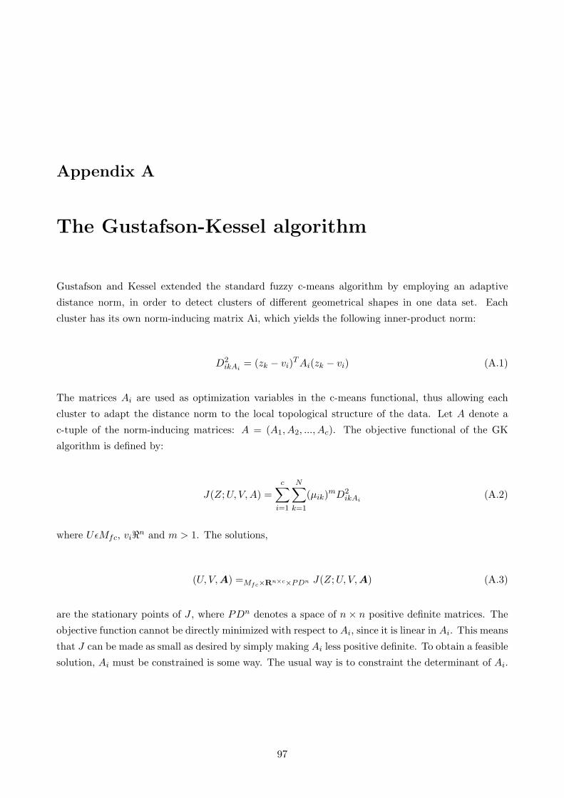
Appendix A
The Gustafson-Kessel algorithm
Gustafson and Kessel extended the standard fuzzy c-means algorithm by employing an adaptive
distance norm, in order to detect clusters of different geometrical shapes in one data set. Each
cluster has its own norm-inducing matrix Ai, which yields the following inner-product norm:
D2ikAi
= (zk − vi)TAi(zk − vi) (A.1)
The matrices Ai are used as optimization variables in the c-means functional, thus allowing each
cluster to adapt the distance norm to the local topological structure of the data. Let A denote a
c-tuple of the norm-inducing matrices: A = (A1, A2, ..., Ac). The objective functional of the GK
algorithm is defined by:
J(Z;U, V,A) =c∑
i=1
N∑k=1
(µik)mD2ikAi
(A.2)
where UεMfc, vi<n and m > 1. The solutions,
(U, V,A) =Mfc×Rn×c×PDn J(Z;U, V,A) (A.3)
are the stationary points of J , where PDn denotes a space of n × n positive definite matrices. The
objective function cannot be directly minimized with respect to Ai, since it is linear in Ai. This means
that J can be made as small as desired by simply making Ai less positive definite. To obtain a feasible
solution, Ai must be constrained is some way. The usual way is to constraint the determinant of Ai.
97
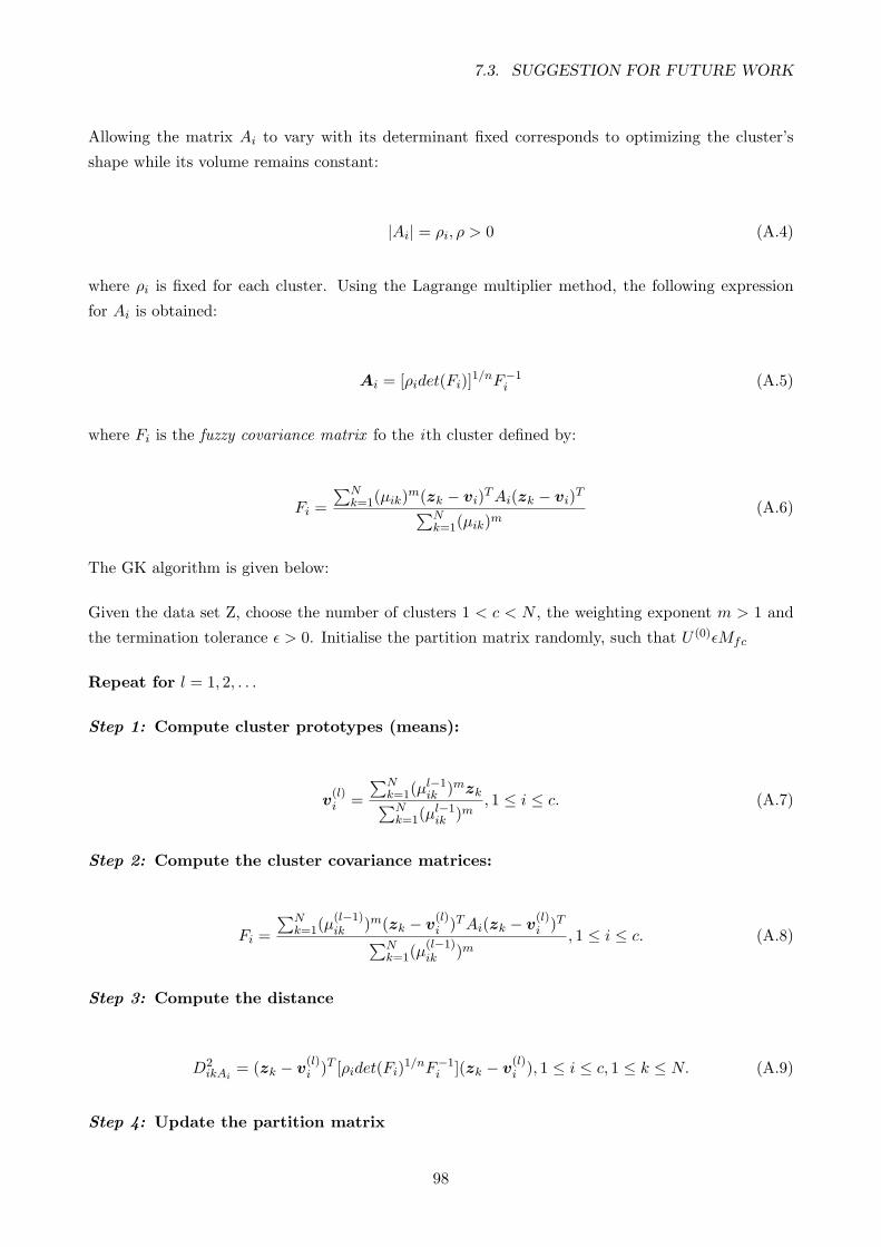
7.3. SUGGESTION FOR FUTURE WORK
Allowing the matrix Ai to vary with its determinant fixed corresponds to optimizing the cluster’s
shape while its volume remains constant:
|Ai| = ρi, ρ > 0 (A.4)
where ρi is fixed for each cluster. Using the Lagrange multiplier method, the following expression
for Ai is obtained:
Ai = [ρidet(Fi)]1/nF−1i (A.5)
where Fi is the fuzzy covariance matrix fo the ith cluster defined by:
Fi =∑N
k=1(µik)m(zk − vi)TAi(zk − vi)T∑Nk=1(µik)m
(A.6)
The GK algorithm is given below:
Given the data set Z, choose the number of clusters 1 < c < N , the weighting exponent m > 1 and
the termination tolerance ε > 0. Initialise the partition matrix randomly, such that U (0)εMfc
Repeat for l = 1, 2, . . .
Step 1: Compute cluster prototypes (means):
v(l)i =
∑Nk=1(µ
l−1ik )mzk∑N
k=1(µl−1ik )m
, 1 ≤ i ≤ c. (A.7)
Step 2: Compute the cluster covariance matrices:
Fi =∑N
k=1(µ(l−1)ik )m(zk − v
(l)i )TAi(zk − v
(l)i )T∑N
k=1(µ(l−1)ik )m
, 1 ≤ i ≤ c. (A.8)
Step 3: Compute the distance
D2ikAi
= (zk − v(l)i )T [ρidet(Fi)1/nF−1
i ](zk − v(l)i ), 1 ≤ i ≤ c, 1 ≤ k ≤ N. (A.9)
Step 4: Update the partition matrix
98

7.3. SUGGESTION FOR FUTURE WORK
if DikAi> 0 for 1 ≤ i ≤ c, 1 ≤ k ≤ N ,
µ(l)ik =
1∑cikAi
(DikAi/DjkAi
)2/(m−1)(A.10)
otherwise
µ(l)ik = 0 if DikAi
> 0 and µ(l)ik ε[0, 1] with
∑ci=1 µ
(l)ik = 1.
until ||U (l) − U (l−1)|| < ε.
99
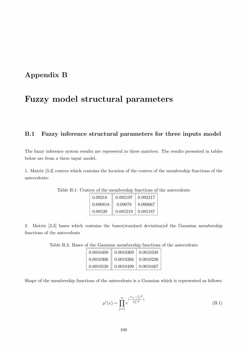
Appendix B
Fuzzy model structural parameters
B.1 Fuzzy inference structural parameters for three inputs model
The fuzzy inference system results are represeted in three matrices. The results presented in tables
below are from a three input model,
1. Matrix [3,3] centres which contains the location of the centres of the membership functions of the
antecedents:
Table B.1: Centres of the membership functions of the antecedents
0.09218 0.092197 0.092217
0.090818 0.09078 0.090667
0.08539 0.085219 0.085187
2. Matrix [3,3] bases which contains the bases(standard deviation)of the Gaussian membership
functions of the antecedents
Table B.2: Bases of the Gaussian membership functions of the antecedents
0.0010408 0.0010369 0.0010338
0.0010306 0.0010266 0.0010236
0.0010538 0.0010499 0.0010467
Shape of the membership functions of the antecedents is a Gaussian which is represented as follows:
µi(x) =n∏
j=1
e((xj−ci
j)2
(bji)2
)
(B.1)
100
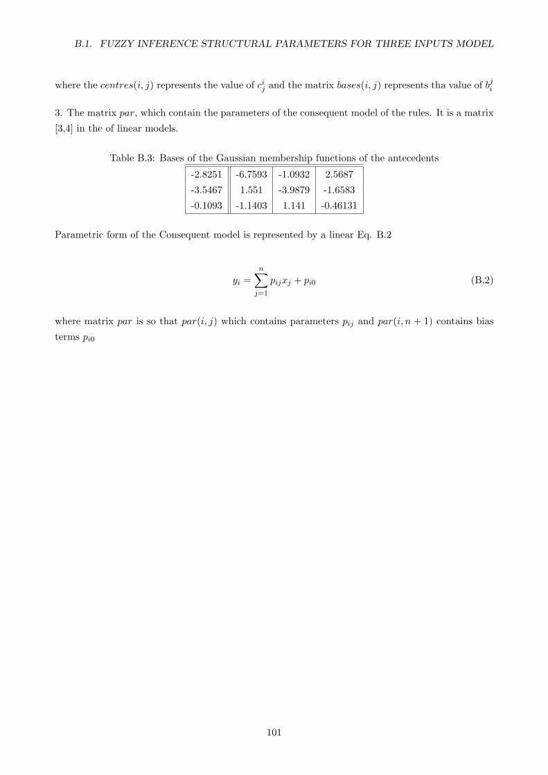
B.1. FUZZY INFERENCE STRUCTURAL PARAMETERS FOR THREE INPUTS MODEL
where the centres(i, j) represents the value of cij and the matrix bases(i, j) represents tha value of bji
3. The matrix par, which contain the parameters of the consequent model of the rules. It is a matrix
[3,4] in the of linear models.
Table B.3: Bases of the Gaussian membership functions of the antecedents
-2.8251 -6.7593 -1.0932 2.5687
-3.5467 1.551 -3.9879 -1.6583
-0.1093 -1.1403 1.141 -0.46131
Parametric form of the Consequent model is represented by a linear Eq. B.2
yi =n∑
j=1
pijxj + pi0 (B.2)
where matrix par is so that par(i, j) which contains parameters pij and par(i, n + 1) contains bias
terms pi0
101
Appendix C
Accuracy methods
C.1 Mean Absolute Percent Error
Mean absolute percentage error (also known as MAPE) is measure of accuracy in a fitted time series
value in statistics, specifically trending. The accuracy expressed as a percentage. It is represted by
the equation shown in Eq.C.1
Error =1n
n∑i=1
|Xi − Fi
Xi| × 100 (C.1)
The difference between actual value X and the forecast value F , is divided by the actual value X
again. The absolute value of this calculation is summed for every fitted or forecast point in time and
divided again by the number of fitted points n. This makes it a percentage error so one can compare
the error of fitted time series that differ in level.
Although the concept of MAPE sound very simple and convincing it has two major drawbacks in
practical application:
1. If there are zero values a division by zero occurs
2. When having a perfect fit, MAPE is zero. MAPE has no restricion in regard to its upper level.
When calculating the average MAPE for a number of time series there might be a problem: a few
number of series that have a very high MAPE might distort a comparison between the average MAPE
of time series fitted with one method compared to the average MAPE when using another method.
In order to avoid this problem other measures have been defined, for example the symmetrical MAPE
(sMAPE) or a relative measure of accuracy.
102
C.2. MSE
Symmetrical MAPE is represeted with an equation shown in Eq.C.2
Error =∑ |X − F |
(X + F )/2× 100 (C.2)
where X is the real value and F is the forecast. By using sMAPE, the problem of large errors when
actual and X, values are close to zero and large difference between absolute percentage errors when
X is greater than F and vice versa. In addition, sMAPE fluctuates between 200% and -200% while
non-symmetric measure does not have limits.
C.2 MSE
Error =1N
n∑i
(xi − yi)2 (C.3)
where xi and yi are the values of the ith samples in x (predicted value) and y (target value),
respectively and N is the number of instances.
C.3 RMSE
Error =
√∑ni=1(xi − yi)2
N(C.4)
where xi and yi are the values of the ith samples in x (predicted value) and y (target value),
respectively and N is the number of instances.
C.4 MSRE
Error =1N
n∑i
(xi − yi
xi)2 (C.5)
where xi and yi are the values of the ith samples in x (predicted value) and y (target value),
respectively and N is the number of instances.
103
C.5. ANDERSON-DARLINGTON
C.5 Anderson-Darlington
AD is represented in functional form shown in Eq C.6:
AD = Σni=1
1− 2in
ln(Fo[Z(i)]) + ln(1− Fo[Zn+1−i] (C.6)
where Fo is the assumed distribution with assumed or sample estimated parameters (µ, σ); Z(i) is
the ith sorted, standardised, sample value; n is the sample size; ln is the natural logarithm (base e)
and subscript i runs from 1 to n.
The null hypothesis, that the true distribution is Fo with the assumed parameters, is then rejected
(at significance level α = 0.05, for sample size n) if the AD test statistic is greater than the critical
value (CV).
Step by step summary of AD GoF test for Normalty
1. Sort original sample and standardise: Z = x−µσ
2. Establish a null hypothesis: assume a normal (µ, σ) distribution
3. Obtain the distribution parameters
4. Obtain the F (Z) cumulative distribution
5. Obtain the logarithm of F (Z); ln(F (Z))
6. Sort the cumulative probability F (Z) in descending order (n− i+ 1)
7. Find the Values of 1− F (Z)
8. Find the logarithm for the above: ln(1− F (Z))
9. Evaluate test statistics AD and CV
10. If CV is greater than AD assume the distribution is normal
104
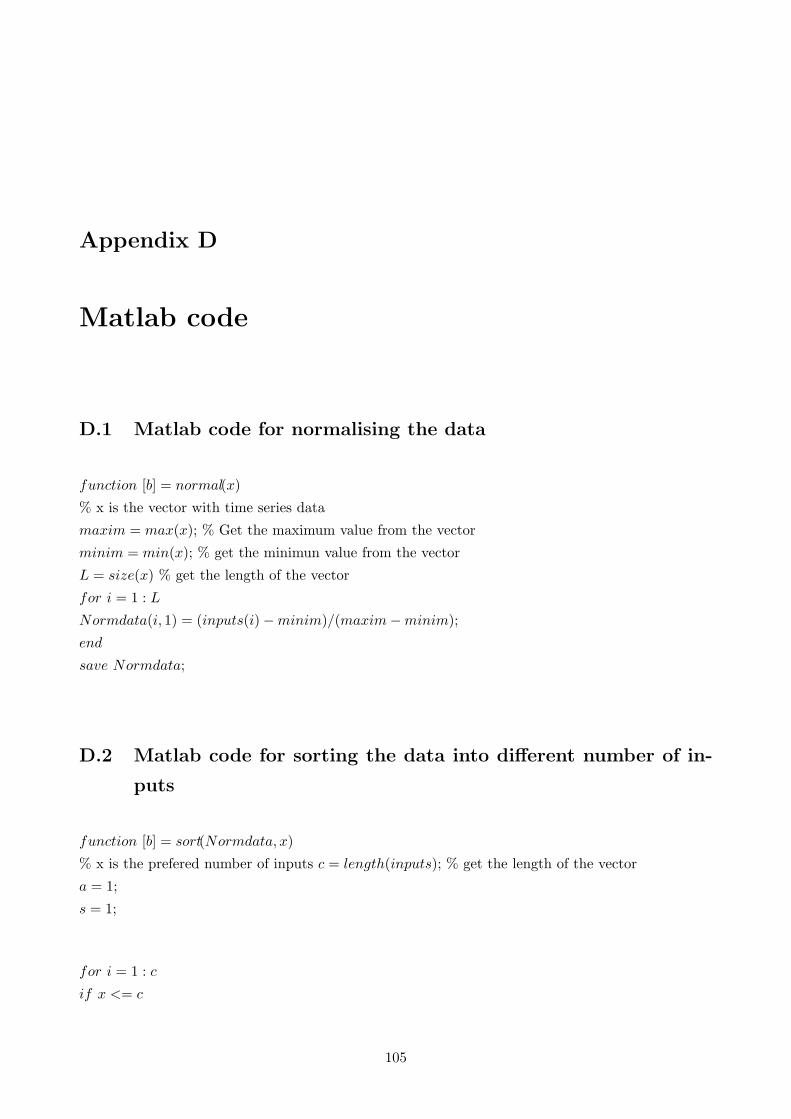
Appendix D
Matlab code
D.1 Matlab code for normalising the data
function [b] = normal(x)
% x is the vector with time series data
maxim = max(x); % Get the maximum value from the vector
minim = min(x); % get the minimun value from the vector
L = size(x) % get the length of the vector
for i = 1 : L
Normdata(i, 1) = (inputs(i)−minim)/(maxim−minim);
end
save Normdata;
D.2 Matlab code for sorting the data into different number of in-
puts
function [b] = sort(Normdata, x)
% x is the prefered number of inputs c = length(inputs); % get the length of the vector
a = 1;
s = 1;
for i = 1 : c
if x <= c
105
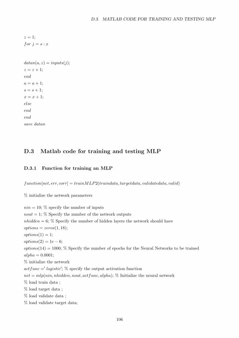
D.3. MATLAB CODE FOR TRAINING AND TESTING MLP
z = 1;
for j = s : x
datan(a, z) = inputs(j);
z = z + 1;
end
a = a+ 1;
s = s+ 1;
x = x+ 1;
else
end
end
save datan
D.3 Matlab code for training and testing MLP
D.3.1 Function for training an MLP
function[net, err, corr] = trainMLP2(traindata, targetdata, validatedata, valid)
% initialize the network parameters
nin = 10; % specify the number of inputs
nout = 1; % Specify the number of the network outputs
nhidden = 6; % Specify the number of hidden layers the network should have
options = zeros(1, 18);
options(1) = 1;
options(2) = 1e− 6;
options(14) = 1000; % Specify the number of epochs for the Neural Networks to be trained
alpha = 0.0001;
% initialize the network
actfunc =′ logistic′; % specify the output activation function
net = mlp(nin, nhidden, nout, actfunc, alpha); % Initialize the neural network
% load train data ;
% load target data ;
% load validate data ;
% load validate target data;
106

D.3. MATLAB CODE FOR TRAINING AND TESTING MLP
% optimization the network
alg =′ scg′; % Specify the optimisation technique, scg(Scaled Conjugate gradient descent)
[net, options] = netopt(net, options, traindata, targetdata, alg); % netopt is a function trains the net-
work with the parameters specied during initialization.
savetrainMLPnetnet; % save the trained model
error = options(8); % get the training error
saveerror
vten = mlpfwd(net, validatedata); % mlpfwd is a function that is used for validating and testing
the trained network
savevten; % save the validation results
[errorv, corr] = errorMLP (v, valid); % errorMLP calculates the RMSE of the validation results
saveerrorv
D.3.2 Netop function used for training the network
function[net, options, varargout] = netopt(net, options, x, t, alg);
% NETOPT Optimize the weights in a network model.
%
%
% [NET, OPTIONS] = NETOPT(NET, OPTIONS, X, T, ALG) takes a network
% data structure NET, together with a vector OPTIONS of parameters
% governing the behaviour of the optimization algorithm, a matrix X of
% input vectors and a matrix T of target vectors, and returns the
% trained network as well as an updated OPTIONS vector. The string ALG
% determines which optimization algorithm (CONJGRAD, QUASINEW, SCG,
% etc.) or Monte Carlo algorithm (such as HMC) will be used.
%
% [NET, OPTIONS, VARARGOUT] = NETOPT(NET, OPTIONS, X, T, ALG) also
% returns any additional return values from the optimisation algorithm.
%
optstring = [alg, ’(”neterr”, w, options, ”netgrad”, net, x, t)’];
% Extract weights from network as single vector
w = netpak(net);
% Carry out optimisation
107

D.3. MATLAB CODE FOR TRAINING AND TESTING MLP
[s1 : nargout] = eval(optstring);
w = s1;
if nargout > 1
options = s2;
% If there are additional arguments, extract them
nextra = nargout− 2;
if nextra > 0
for i = 1 : nextra
varargouti = si+ 2;
end
end
end
% Pack the weights back into the network
net = netunpak(net, w);
subsectionmlpfwd function for validating and testing the network
function[y, z, a] = mlpfwd(net, x)
%MLPFWD Forward propagation through 2-layer network.
% % Description
% Y = MLPFWD(NET, X) takes a network data structure NET together with a
% matrix X of input vectors, and forward propagates the inputs through
% the network to generate a matrix Y of output vectors. Each row of X
% corresponds to one input vector and each row of Y corresponds to one
% output vector.
% [Y, Z] = MLPFWD(NET, X) also generates a matrix Z of the hidden unit
% activations where each row corresponds to one pattern.
% [Y, Z, A] = MLPFWD(NET, X) also returns a matrix A giving the summed
% inputs to each output unit, where each row corresponds to one
% pattern.
% Check arguments for consistency
errstring = consist(net,′mlp′, x);
if isempty(errstring);
error(errstring);
108

D.3. MATLAB CODE FOR TRAINING AND TESTING MLP
end
ndata = size(x, 1);
z = tanh(x ∗ net.w1 + ones(ndata, 1) ∗ net.b1);
a = z ∗ net.w2 + ones(ndata, 1) ∗ net.b2;
switch net.outfn
case ′linear′ % Linear outputs
y = a;
case′logistic′ % Logistic outputs
% Prevent overflow and underflow: use same bounds as mlperr
% Ensure that log(1-y) is computable: need exp(a) ¿ eps
maxcut = −log(eps);% Ensure that log(y) is computable
mincut = −log(1/realmin− 1);
y = 1./(1 + exp(−a));
case′softmax′ % Softmax outputs
% Prevent overflow and underflow: use same bounds as glmerr
% Ensure that sum(exp(a), 2) does not overflow
maxcut = log(realmax)− log(net.nout);
% Ensure that exp(a) ¿ 0
mincut = log(realmin);
a = min(a,maxcut);
a = max(a,mincut);
temp = exp(a);
y = temp./(sum(temp, 2) ∗ ones(1, net.nout));
109
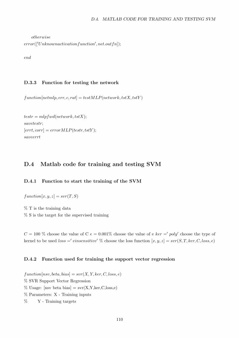
D.4. MATLAB CODE FOR TRAINING AND TESTING SVM
otherwise
error([′Unknownactivationfunction′, net.outfn]);
end
D.3.3 Function for testing the network
function[netmlp, err, c, rat] = testMLP (network, tstX, tstY )
testr = mlpfwd(network, tstX);
savetestr;
[errt, corr] = errorMLP (testr, tstY );
saveerrt
D.4 Matlab code for training and testing SVM
D.4.1 Function to start the training of the SVM
function[x, y, z] = svr(T, S)
% T is the training data
% S is the target for the supervised training
C = 100 % choose the value of C e = 0.001% choose the value of e ker =′ poly′ choose the type of
kernel to be used loss =′ einsensitive′ % choose the loss function [x, y, z] = svr(S, T, ker, C, loss, e)
D.4.2 Function used for training the support vector regression
function[nsv, beta, bias] = svr(X,Y, ker, C, loss, e)
% SVR Support Vector Regression
% Usage: [nsv beta bias] = svr(X,Y,ker,C,loss,e)
% Parameters: X - Training inputs
% Y - Training targets
110

D.4. MATLAB CODE FOR TRAINING AND TESTING SVM
% ker - kernel function
% C - upper bound (non-separable case)
% loss - loss function
% e - insensitivity
% nsv - number of support vectors
% beta - Difference of Lagrange Multipliers
% bias - bias term
if(nargin < 3|nargin > 6) % check correct number of arguments
helpsvr
else
fprintf(′SupportV ectorRegressing....′)
fprintf(′
n = size(X,1);
if (nargin¡6) e=0.0;, end
if (nargin¡5) loss=’eInsensitive’;, end
if (nargin¡4) C=Inf;, end
if (nargin¡3) ker=’linear’;, end
% tolerance for Support Vector Detection
epsilon = svtol(C);
% Construct the Kernel matrix
fprintf(′Constructing...);
H = zeros(n, n);
fori = 1 : n
forj = 1 : n
H(i, j) = svkernel(ker,X(i, :), X(j, :));
end
end
% Set up the parameters for the Optimisation problem
switchlower(loss)
case′einsensitive′,
Hb = [H −H;−HH];
c = [(e ∗ ones(n, 1)− Y ); (e ∗ ones(n, 1) + Y )];
vlb = zeros(2 ∗ n, 1); % Set the bounds: alphas ¿= 0
111

D.4. MATLAB CODE FOR TRAINING AND TESTING SVM
vub = C ∗ ones(2 ∗ n, 1); % alphas ¡= C
x0 = zeros(2 ∗ n, 1); % The starting point is [0 0 0 0]
neqcstr = nobias(ker); % Set the number of equality constraints (1 or 0)
ifneqcstr A = [ones(1, n)− ones(1, n)]; , b = 0; % Set the constraint Ax = b
else
A = []; , b = [];
end
case′quadratic′,
Hb = H + eye(n)/(2 ∗ C);
c = −Y ;
vlb = −1e30 ∗ ones(n, 1);
vub = 1e30 ∗ ones(n, 1);
x0 = zeros(n, 1); % The starting point is [0 0 0 0]
neqcstr = nobias(ker); % Set the number of equality constraints (1 or 0)
ifneqcstr
A = ones(1, n); , b = 0; % Set the constraint Ax = b
else
A = []; , b = [];
end
otherwise, disp(′Error : Unknown Loss Function′);
end
% Add small amount of zero order regularisation to
% avoid problems when Hessian is badly conditioned.
% Rank is always less than or equal to n.
% Note that adding to much reg will peturb solution
Hb = Hb+ 1e− 10 ∗ eye(size(Hb));
% Solve the Optimisation Problem
fprintf(′Optimising...);
st = cputime;
[alpha lambda how] = qp(Hb, c,A, b, vlb, vub, x0, neqcstr);
112
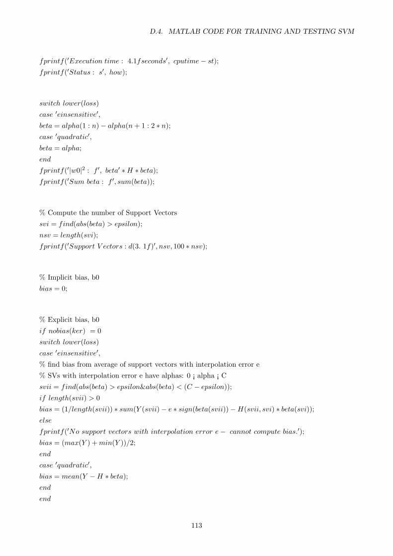
D.4. MATLAB CODE FOR TRAINING AND TESTING SVM
fprintf(′Execution time : 4.1fseconds′, cputime− st);
fprintf(′Status : s′, how);
switch lower(loss)
case ′einsensitive′,
beta = alpha(1 : n)− alpha(n+ 1 : 2 ∗ n);
case ′quadratic′,
beta = alpha;
end
fprintf(′|w0|2 : f ′, beta′ ∗H ∗ beta);fprintf(′Sum beta : f ′, sum(beta));
% Compute the number of Support Vectors
svi = find(abs(beta) > epsilon);
nsv = length(svi);
fprintf(′Support V ectors : d(3. 1f)′, nsv, 100 ∗ nsv);
% Implicit bias, b0
bias = 0;
% Explicit bias, b0
if nobias(ker) = 0
switch lower(loss)
case ′einsensitive′,
% find bias from average of support vectors with interpolation error e
% SVs with interpolation error e have alphas: 0 ¡ alpha ¡ C
svii = find(abs(beta) > epsilon&abs(beta) < (C − epsilon));
if length(svii) > 0
bias = (1/length(svii)) ∗ sum(Y (svii)− e ∗ sign(beta(svii))−H(svii, svi) ∗ beta(svi));else
fprintf(′No support vectors with interpolation error e− cannot compute bias.′);
bias = (max(Y ) +min(Y ))/2;
end
case ′quadratic′,
bias = mean(Y −H ∗ beta);end
end
113

D.5. MATLAB CODE FOR TRAINING AND TESTING NEUROFUZZY
end
D.4.3 Function for Validating and testing the constructed SVR model
function [r] = test(X,Y, beta, bias)
ker =′ poly′; r = svroutput(X,Y, ker, beta, bias); saver
D.5 Matlab code for training and testing Neurofuzzy
D.5.1 Function for training the Neurofuzzy
function = trainNF (x)
y = fuzzy b % fuzzy-b is the function on the toolbox that used to train the network
D.5.2 Function fuzz-b used to train the Neuro=fuzzy
global model
global memb fun
global model bias
global arch
global format out
global init
global no sets
global mod id
global mod path
global mhist id
global mhist path
global err id
114

D.5. MATLAB CODE FOR TRAINING AND TESTING NEUROFUZZY
global err path
global ehist id
global ehist path
global pred id
global pred path
global memo id
global memo path
current dir = pwd;
c = computer;
if isunix
current dir = [current dir,′′ ];
else
if strcmp(c(1 : 2),′ PC ′)
current dir = [current dir,′′ ];
end
if strcmp(c(1 : 2),′MA′)
current dir = [current dir,′ :′];
end
end
% The ’data’ (the training set) matrix is stored in the file:
data id =′ data.mat′;
data path = current dir;
% Save the memoranda in the file:
memo id =′ memoid′;
memo path = current dir;
% Train one model of given complexity or find the best complexity?
pr =′ evaluate′;
%%%for model training only
% complexity
115

D.5. MATLAB CODE FOR TRAINING AND TESTING NEUROFUZZY
comp = 5;
% Save the trained model in the file:
mod id =′ model.mat′;
mod path = current dir;
% Save the computation diary in the file:
mhist id =′ mhist.txt′;
mhist path = current dir;
% for model evaluating only % The trained model is stored in the file: tmod id =′ model.mat′;
tmod path = current dir;
% The ’in’ (test set) matrix is stored in the file: in id =′ in.mat′; in path = current dir; % Save the
predicted output in the file: pred id =′ out hat.mat′; pred path = current dir;
% for complexity-error exploration only
% range of complexity
comp min = 10;
comp max = 20;
% validation
valid =′ xvalid′;
% no sets x valid
no sets = 10;
% Save the error Vs complexity matrix in the file:
err id =′ errors.mat′;
err path = current dir;
% Save the computation diary in the file:
ehist id =′ ehist.txt′;
ehist path = current dir;
% model type
model =′ fuz′;
% for complexity-error exploration and model training only:
% form of membership functions
memb fun =′ gaussian′;
% for complexity-error exploration and model training only:
% Bias model bias =′ no bias′;
116

D.5. MATLAB CODE FOR TRAINING AND TESTING NEUROFUZZY
% for complexity-error exploration and model training only:
% architecture
arch =′ comb′;
% for complexity-error exploration and model training only:
% format out
formatout =′ linear′;
% cluster: initialization of the centers and bases
init =′ HFC ′;
if strcmp(pr, ′one mod′)
eval([′load′, data path, data id]); fuz aux(pr, comp, data);
elseif strcmp(pr,′ evaluate′)
eval([′load′, tmod path, tmod id]);
eval([′load′, in path, in id]);
fuz aux(pr, centers, bases, par, bias, in);
elseif strcmp(pr,′ comp err′)
eval([′load′, datapath, dataid]);
fuz aux(pr, comp min, comp max, data);
end
clear model valid memb fun model bias
clear arch format out init no sets
clear mod id mod path mhist id mhist path
clear err id err path ehist id ehist path
clear pred id pred path in id in path
clear tmod id tmod path
clear memoid memo path
clear pr
clear centers bases par bias in
clear comp comp min comp max
clear data data id data path
clear c current dir
117

D.5. MATLAB CODE FOR TRAINING AND TESTING NEUROFUZZY
D.5.3 A function for identifying the parameters of the fuzzy model
function[centers, bases, par, bias] = fuz − id(comp, training − set)
%FUZ-ID Identification of the parameters of a Fuzzy Model
% [centers,bases,par,bias]=fuz-id(comp,training-set)
% centers[no-rules,no-var]
% bases[no-rules,no-var]
% par[no-rules,no-par] where no-par=1 if model=’constant’
% and no-par=no-var+1 if model=’linear’
% bias[1,1]
% comp[1,1] is the complexity of the model being identified
% training-set[no-data,no-var+1] the first no-var columns are the
% inputs, the last one is the output
% The following global variable are required:
% memb-fun: ’gaussian’/’triangular’
% arch: ’weigthed’/’comb’
% format-out: ’linear’/’constant’
% init: ’k-mean’/’hfc’
% fid-h
global memb fun
global arch
global format out
global init
global fid h
%Initialization:
[centers, bases] = eval([init′(comp, training set)′]);
%Optimization:
termination = 0;
oldSSE = 1e+ 10;
k = 0.005;
[nodata, c] = size(training set);
118

D.5. MATLAB CODE FOR TRAINING AND TESTING NEUROFUZZY
intrn = training set(:, 1 : c− 1);
outtrn = training set(:, c);
while(termination < 2)
% INVERSION to determine the parameters of the CONSEQUENTS
if strcmp(formatout,′ constant′) [SSE, newpar, bias] = invco(intrn, centers, bases, outtrn);
end
if strcmp(formatout,′ linear′)
[SSE, newpar, bias] = invli(intrn, centers, bases, outtrn);
end
if (SSE/old SSE > 1− k)
termination = termination+ 1;
end
if isnan(SSE)
break;
end
par = newpar;
fprintf(fidh,′Consequents optimization.SSE =%g′, SSE);
oldSSE = SSE;
% LEVENBERG-MARQUARDT to determine the CENTERS and the BASES
[centers, bases] = levemao(intrn, centers, bases, par, bias, outtrn);
end
function [centers, bases] = levemao(inputs, centers, bases, par, bias, output)
% LEVEMAO LEVEMBERG-MARQUARDT
% [centers, bases]=levemao(inputs,centers,bases,par,output)
% centers[norules,novar] centers of the membership functions
% bases[norules,novar] bases of the membership functions
119

D.5. MATLAB CODE FOR TRAINING AND TESTING NEUROFUZZY
% inputs[nodata,novar] % centers[norules,novar] centers (initial value)
% bases[norules,novar] bases (initial value)
% par[norules,nopar] parameters of the consequent of each rule
% bias[1,1]
% output[nodata,1]
% The following global variable is required: fidh
% LEVENBERG-MARQUARDT is used to determine the CENTERS and the BASES
global fidh
me = 3;
gradmin = .25;
muinit = 0.001;
muinc = 10;
mudec = 0.1;
mumax = 1e10;
nodata = size(inputs, 1);
[norules, novar] = size(centers);
mu = muinit;
[errors, Jacobian] = errfuz(inputs, centers, bases, par, bias, output);
premise = [centers(:); bases(:)];
SSE = sumsqr(errors);
message = sprintf(’Premise optimization: fprintf(fidh,message, 0,muinit, SSE);
fori = 1 : me
% CHECK MAGNITUDE OF GRADIENT
if(norm(Jacobian′ ∗ errors)/nodata < gradmin), break, end
% INNER LOOP, INCREASE MU UNTIL THE ERRORS ARE REDUCED
while(mu <= mumax)
H = Jacobian′ ∗ Jacobian;
g = Jacobian′ ∗ errors;A = H +mu ∗ no data ∗ eye(2 ∗ norules ∗ novar);
120

D.5. MATLAB CODE FOR TRAINING AND TESTING NEUROFUZZY
tol = 1e− 9;
newpremise = premise− pinv(A, tol) ∗ g;
centers = reshape(newpremise(1 : novar ∗ norules), [norules novar]);
bases = reshape(newpremise(novar ∗ norules+ 1 : 2 ∗ novar ∗ norules), [norules novar]);
bases = bases+ (bases < 0.1) ∗ 0.1;
% EVALUATE NEW NETWORK
[newerrors, newJacobian] = errfuz(inputs, centers, bases, par, bias, output);
newSSE = sumsqr(new errors);
if(newSSE < SSE), break, end
mu = mu ∗muinc;end
if(mu > mumax), break, end
mu = mu ∗mudec;
% UPDATE NETWORK
premise = newpremise;
SSE = newSSE;
Jacobian = newJacobian;
fprintf(fidh,message, i,mu, SSE);
end
D.5.4 function for computing the output of the Neurofuzzy model
functionout = fuz −mod(inputs, centers, bases, par, bias)
% FUZ-MOD
% out=fuz mod(inputs,centers,bases,par,bias)
% out[n data,1]
% inputs[no data,no var]
121

D.5. MATLAB CODE FOR TRAINING AND TESTING NEUROFUZZY
% centers[no rules,no var] centers of the membership functions
% bases[no-rules,no var] bases of the membership functions
% par[no rules,no par] parameters of the consequent of each rule
% bias[1,1]
% Given an input matrix and the matrices centers, bases, par and bias,
% fuz-mod returns the corresponding output of the fuzzy system
% The following global variable are required:
% memb-fun: ’gaussian’/’triangular’ % arch: ’weigthed’/’comb’ % format-out: ’linear’/’constant’
global memb fun;
global arch;
global format out;
[no data, no var] = size(inputs);
[no rules, no var] = size(centers);
[no rules, no par] = size(par);
if strcmp(format out,′ linear′)
y = [inputs, ones(no data, 1)] ∗ par′;end
if strcmp(format out,′ constant′)
y = ones(no data, 1) ∗ par′;end
Sum w = zeros(no data, 1);
Sum wy = zeros(no data, 1);
for i = 1 : no rules
w = ones(no data, 1); %initialization of the degree of match
%of the inputs to the premise of the i-th rule
for j = 1 : no var
%match[no data,1] is the degree of match of each
122
D.5. MATLAB CODE FOR TRAINING AND TESTING NEUROFUZZY
%datum to the premise of the i-th rule for what
%concerns the j-th direction of the input space
if strcmp(memb fun,′ gaussian′)
match = exp(−((inputs(:, j)− centers(i, j)).2)/bases(i, j));
end
if strcmp(memb fun,′ triangular′)
match = max(0, ones(no data, 1)− 2 ∗ abs(inputs(:, j)− centers(i, j))/bases(i, j));
end
w = w. ∗match;end
Sum wy = Sum wy + w. ∗ y(:, i);Sum w = Sum− w + w;
end
Sum w = Sum w + (Sum w == 0); % if Sum w = 0 then Sun w = 1
% n.b. in this case Sum wy = 0
if strcmp(arch,′weigthed′)
out = Sum wy./Sum w;
end
if strcmp(arch,′ comb′)
out = Sum wy;
end
out = out+ bias ∗ ones(size(out));
123
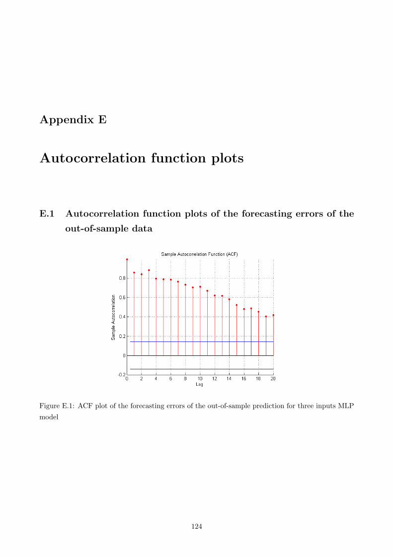
Appendix E
Autocorrelation function plots
E.1 Autocorrelation function plots of the forecasting errors of the
out-of-sample data
Figure E.1: ACF plot of the forecasting errors of the out-of-sample prediction for three inputs MLP
model
124
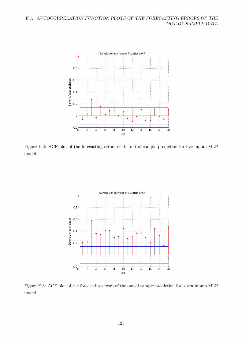
E.1. AUTOCORRELATION FUNCTION PLOTS OF THE FORECASTING ERRORS OF THEOUT-OF-SAMPLE DATA
Figure E.2: ACF plot of the forecasting errors of the out-of-sample prediction for five inputs MLP
model
Figure E.3: ACF plot of the forecasting errors of the out-of-sample prediction for seven inputs MLP
model
125
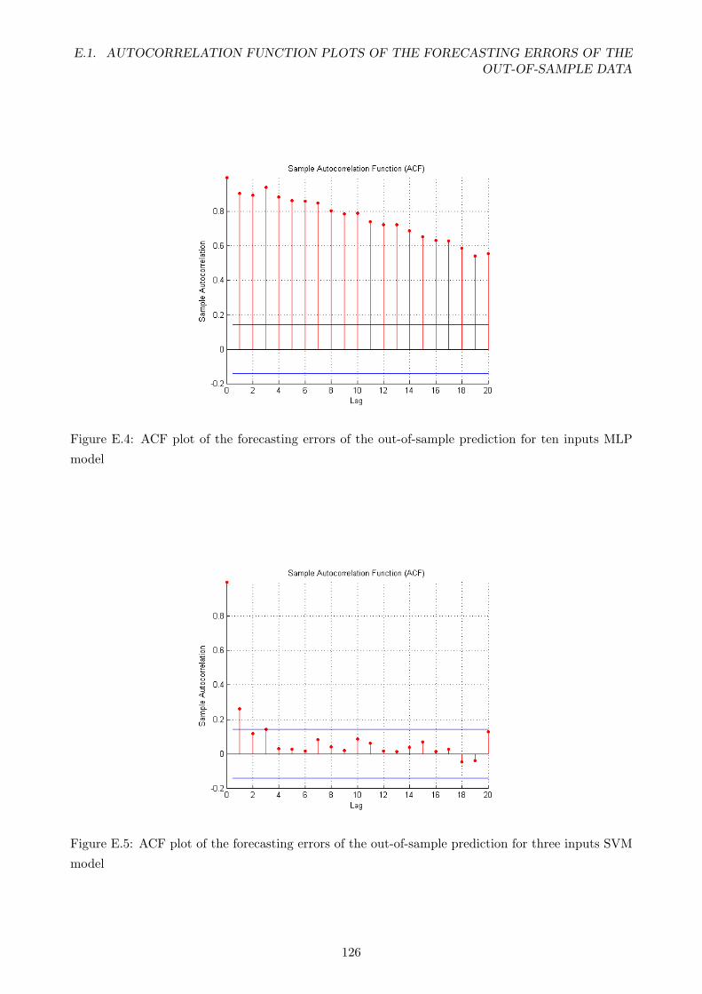
E.1. AUTOCORRELATION FUNCTION PLOTS OF THE FORECASTING ERRORS OF THEOUT-OF-SAMPLE DATA
Figure E.4: ACF plot of the forecasting errors of the out-of-sample prediction for ten inputs MLP
model
Figure E.5: ACF plot of the forecasting errors of the out-of-sample prediction for three inputs SVM
model
126
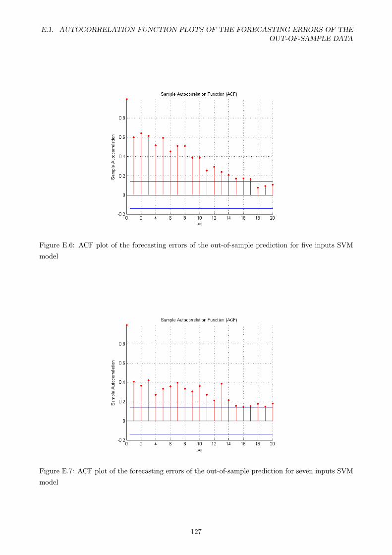
E.1. AUTOCORRELATION FUNCTION PLOTS OF THE FORECASTING ERRORS OF THEOUT-OF-SAMPLE DATA
Figure E.6: ACF plot of the forecasting errors of the out-of-sample prediction for five inputs SVM
model
Figure E.7: ACF plot of the forecasting errors of the out-of-sample prediction for seven inputs SVM
model
127
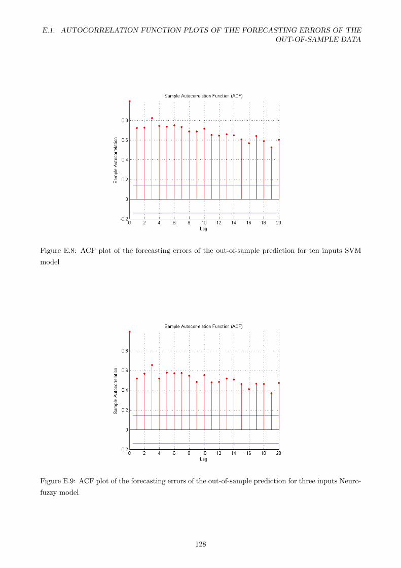
E.1. AUTOCORRELATION FUNCTION PLOTS OF THE FORECASTING ERRORS OF THEOUT-OF-SAMPLE DATA
Figure E.8: ACF plot of the forecasting errors of the out-of-sample prediction for ten inputs SVM
model
Figure E.9: ACF plot of the forecasting errors of the out-of-sample prediction for three inputs Neuro-
fuzzy model
128
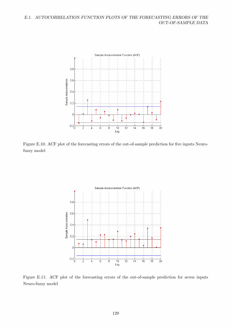
E.1. AUTOCORRELATION FUNCTION PLOTS OF THE FORECASTING ERRORS OF THEOUT-OF-SAMPLE DATA
Figure E.10: ACF plot of the forecasting errors of the out-of-sample prediction for five inputs Neuro-
fuzzy model
Figure E.11: ACF plot of the forecasting errors of the out-of-sample prediction for seven inputs
Neuro-fuzzy model
129

E.1. AUTOCORRELATION FUNCTION PLOTS OF THE FORECASTING ERRORS OF THEOUT-OF-SAMPLE DATA
Figure E.12: ACF plot of the forecasting errors of the out-of-sample prediction for ten inputs Neuro-
fuzzy model
130
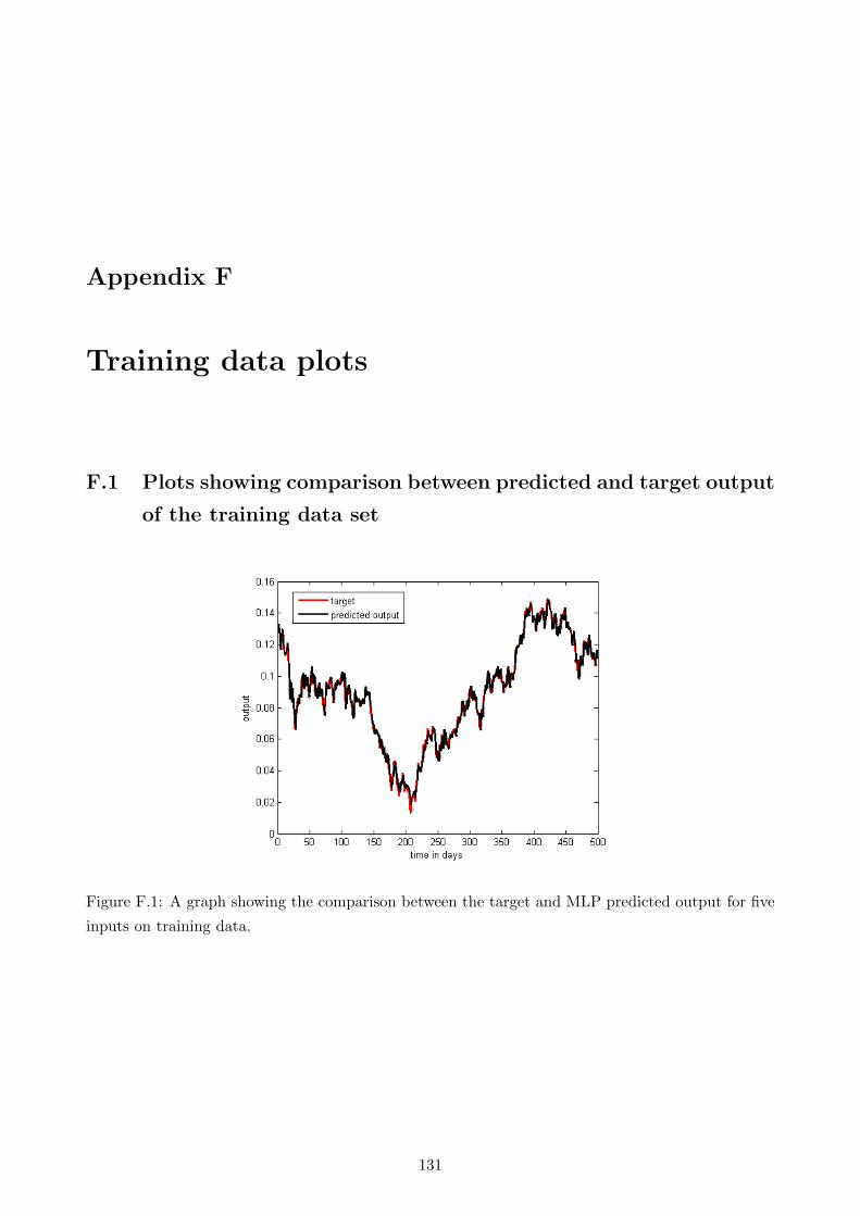
Appendix F
Training data plots
F.1 Plots showing comparison between predicted and target output
of the training data set
Figure F.1: A graph showing the comparison between the target and MLP predicted output for five
inputs on training data.
131

F.1. PLOTS SHOWING COMPARISON BETWEEN PREDICTED AND TARGET OUTPUTOF THE TRAINING DATA SET
Figure F.2: A graph showing the comparison between the target and svm predicted output for three
inputs on training data.
Figure F.3: A graph showing the comparison between the target and Neuro-fuzzy predicted output
for five inputs on training data.
132
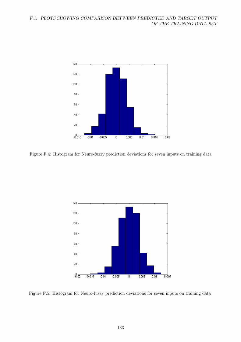
F.1. PLOTS SHOWING COMPARISON BETWEEN PREDICTED AND TARGET OUTPUTOF THE TRAINING DATA SET
Figure F.4: Histogram for Neuro-fuzzy prediction deviations for seven inputs on training data
Figure F.5: Histogram for Neuro-fuzzy prediction deviations for seven inputs on training data
133
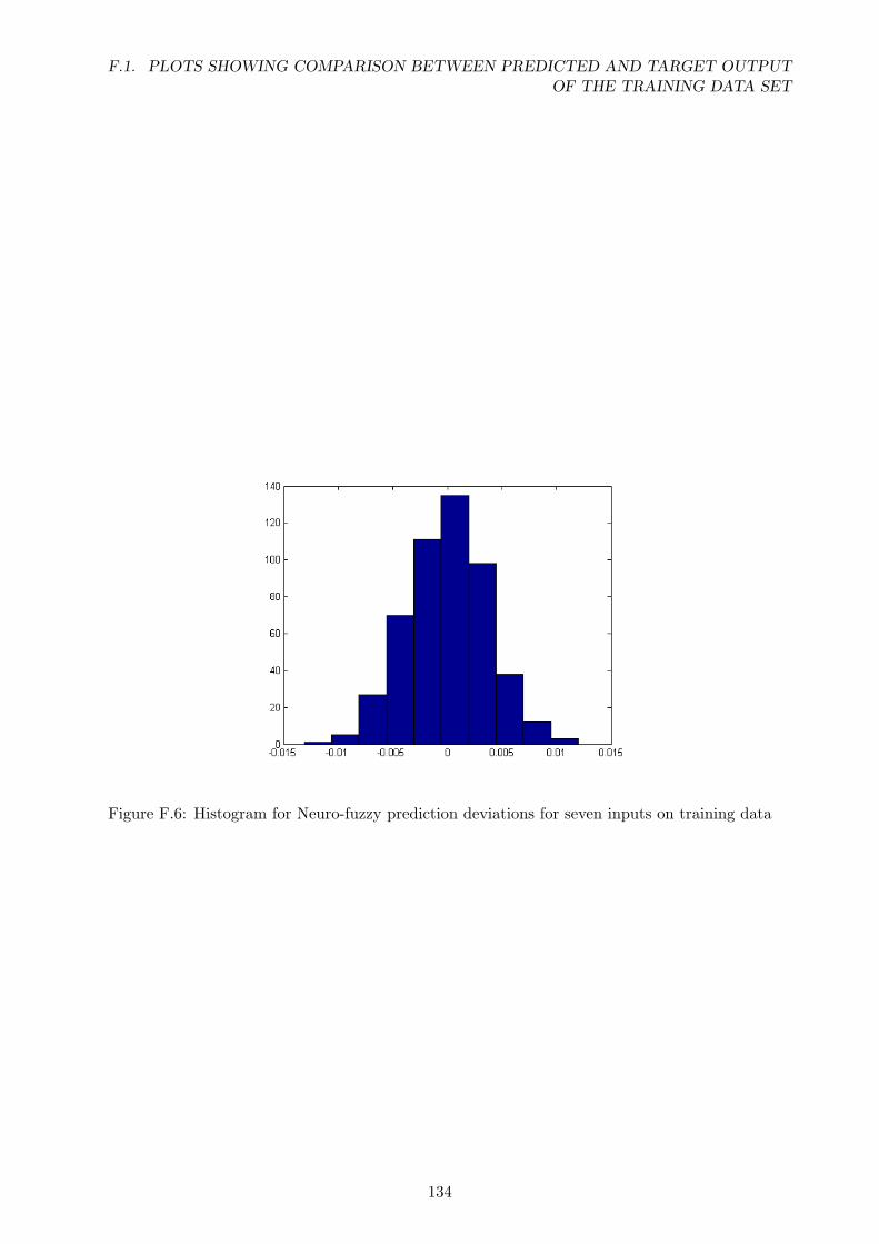
F.1. PLOTS SHOWING COMPARISON BETWEEN PREDICTED AND TARGET OUTPUTOF THE TRAINING DATA SET
Figure F.6: Histogram for Neuro-fuzzy prediction deviations for seven inputs on training data
134

Appendix G
Anderson-Darling test results
G.1 Anderson-Darling test results for forecasting errors
G.1.1 MLP AD test results
Three inputs MLP model forecasting errors:
1. Sample size: 200
2. Anderson-Darling statistic: 5.6425
3. Anderson-Darling adjusted statistic: 5.6640
4. Probability associated to the Anderson-Darling statistic = 0.0000
5. With a given significance = 0.050
6. The sampled population is not normally distributed.
Seven inputs MLP model forecasting errors:
1. Sample size: 200
2. Anderson-Darling statistic: 0.6666
3. Anderson-Darling adjusted statistic: 0.6691
4. Probability associated to the Anderson-Darling statistic = 0.806
5. With a given significance = 0.050
135

G.1. ANDERSON-DARLING TEST RESULTS FOR FORECASTING ERRORS
6. The sampled population is normally distributed.
7. Thus, this sample have been drawn from a normal population with a mean and variance =
0.0064 0.0000
Ten inputs MLP model forecasting errors:
1. Sample size: 200
2. Anderson-Darling statistic: 4.1132
3. Anderson-Darling adjusted statistic: 4.1157
4. Probability associated to the Anderson-Darling statistic = 0.0000
5. With a given significance = 0.050
6. The sampled population is not normally distributed.
G.1.2 SVM AD test results
Five inputs SVM model forecasting errors:
1. Sample size: 200
2. Anderson-Darling statistic: 2.4592
3. Anderson-Darling adjusted statistic: 2.4685
4. Probability associated to the Anderson-Darling statistic = 0.0000
5. With a given significance = 0.050
6. The sampled population is not normally distributed.
Seven inputs model forecasting errors:
1. Sample size: 200
2. Anderson-Darling statistic: 2.5132
3. Anderson-Darling adjusted statistic: 2.5228
4. Probability associated to the Anderson-Darling statistic = 0.0000
136

G.1. ANDERSON-DARLING TEST RESULTS FOR FORECASTING ERRORS
5. With a given significance = 0.050
6. The sampled population is not normally distributed.
Ten inputs SVM model forecasting errors:
1. Sample size: 200
2. Anderson-Darling statistic: 1.1439
3. Anderson-Darling adjusted statistic: 1.1483
4. Probability associated to the Anderson-Darling statistic = 0.0053
5. With a given significance = 0.050
6. The sampled population is not normally distributed.
G.1.3 Neuro-fuzzy AD test results
Three inputs Neurofuzzy model forecasting errors:
1. Sample size: 200
2. Anderson-Darling statistic: 0.7143
3. Anderson-Darling adjusted statistic: 0.7170
4. Probability associated to the Anderson-Darling statistic = 0.0614
5. With a given significance = 0.050
6. The sampled population is normally distributed.
7. Thus, this sample have been drawn from a normal population with a mean and variance =
0.0062 0.0000
Seven inputs Neuro-fuzzy model forecasting errors:
1. Sample size: 200
2. Anderson-Darling statistic: 0.2045
3. Anderson-Darling adjusted statistic: 0.2053
137

G.1. ANDERSON-DARLING TEST RESULTS FOR FORECASTING ERRORS
4. Probability associated to the Anderson-Darling statistic = 0.8723
5. With a given significance = 0.050
6. The sampled population is normally distributed.
7. Thus, this sample have been drawn from a normal population with a mean and variance =
0.0040 0.0000
Ten inputs Neurofuzzy model forecasting errors:
1. Sample size: 200
2. Anderson-Darling statistic: 0.3023
3. Anderson-Darling adjusted statistic: 0.3034
4. Probability associated to the Anderson-Darling statistic = 0.5730
5. With a given significance = 0.050
6. The sampled population is normally distributed.
7. Thus, this sample have been drawn from a normal population with a mean and variance =
0.0048 0.0000
138
References
[1] Kolarik and G. Rudorfer, “Time series forecasting using neural networks, department of ap-
plied computer science,” Vienna University of Economics and Business Administration, no. 1090,
pp. 2–6, 1997.
[2] E. Fama, “The behaviour of stock market prices,” 1965.
[3] E. Fama, Foundations of finance. New York: Basic Books, 1976.
[4] E. Fama, “Efficient capital markets: a review of theory and empirical work,” Journal of Finance,
vol. 25, pp. 383–417, 1970.
[5] M. Jensen, “Some anomalous evidence regarding market efficiency,” Journal of Financial Eco-
nomics, vol. 6, pp. 95–101, 1978.
[6] R. Balvers, T. Cosimano, and B. McDonald, “Predicting stock returns in an efficient market,”
Journal of Finance, vol. 55, pp. 1109–1128, 1990.
[7] H. Kim and K. Shin, “A hybrid approach based on neural networks and genetic algorithms for
detecting temporal patterns in stock markets,” Applied Soft Computing, vol. 7, pp. 569–576, 2007.
[8] S. Makridakis, Wheelwright. and McGEE, FORECASTING: Methods and Applications. John
Wiley and Sons, Inc,second ed, 1997.
[9] S. Makridakis and H. Hibon, “Accuracy of forecasting: An Emperical Investigation” J. Roy
Statist. Soc., no. 8, pp. 69–80, 1992.
[10] L.J. Tashman, “Out-of-sample tests of forecasting accuracy: an analysis and review” Interna-
tional Journal of Forecasting,vol. 7, no. 4, pp. 437–450, 2000.
[11] R. Fieldes and S. Makridakis, “The impact of emperical accuracy studies on time series analysis
forecasting” International Statistical Review, no. 63, pp. 289–308, 1995.
[12] J. Scott Armstrong and C. Kisten Green, “Demand forecasting: Evidence-based Method” A
chapter for the book, ’Strategic Marketing Management: A business Process Approach edited by
Luiz Moutinho and Geoff Southern, 2006.
[13] J. Scott Armstrong and F. Collopy, “Error Measures For Generalizing About Forecasting Meth-
ods: Empirical Comparisons” International Journal of Forecasting, no. 142, pp. 97–125, 1979.
139
REFERENCES
[14] C. Chatfield, “Apples, oranges and mean square error” International Journal of Forecasting,
no. 4, pp. 515–518, 1988.
[15] S. Makridakis, A. Anderson,R. Carbone, R. Fildes, M. Hibon, R. Lewandowski, J. Newton,
E. Parzen, R. Winkler “The accuracy of extrapolation(time series) methods: results of a fore-
casting competition” Journal of Forecasting, no. 1, pp. 111–153, 1982.
[16] C. Chatfield, “Calculating interval forecasts” Journal of Business and Economic Statistics,
no. 11, pp. 121–135, 1993.
[17] S.M. Bartolomei and A.L. Sweet, “A note on the comparison of exponential smoothing methods
for forecasting seasonal series” International Journal of Forecasting, no. 5, pp. 111–116, 1989.
[18] P.N. Pant and W.H. starbuck, “Innocents in the forest: forecasting and research methods”
Journal of Management, no. 16, pp. 433–460, 1990.
[19] A. Timmermann and C. Granger, “Efficient market hypothesis and forecasting” International
Journal of Forecasting, no. 20, pp. 15–27, 2004.
[20] Standard bank, “Basic invesment course,” www.securities.co.za. last accessed on 01 September
2007
[21] Clive.W.J. Granger, “Forecasting stock market prices:Lessons for forecasters,” International
Journal of forecasting, no. 8,pp. 3–13, 1992.
[22] D.J. Reid, “A comparative study of time series prediction techniques on economic data” PhD
thesis, Department of Mathematics, University of Nottingham, ,1969.
[23] P. Newbold and C.W.J. Granger, “Experience with forecasting univariate time series and the
combination of forecasts (with discussion)” Journal of Royal Statistical Society, no. A 137,
pp. 131–165, 1974.
[24] G. Hill and R. Fildes, “The accuracy of extrapolation methods: an automatic Box-Jenkins
package SIFT” Journal of Forecasting, no. 3, pp. 319–323, 1984.
[25] A.B. Koeler and E.S. Murphee, “A comparison of results from state space forecasting with
forecasts from Makridakis competition” International Journal of Forecasting, no. 4, pp. 45–55,
1988.
[26] E.J. Lusk and J.S. Neeves, “A comparative ARIMA analysis of the 111 series of the Makridakis
competition” International Journal of Forecasting, no. 3, pp. 329–332, 1984.
[27] R. Fildes,M. Hibbon, S. Makridakis,and N. Mead, “generalizing about univariate forecasting
methods: further emperical evidence” International Journal of Forecasting, no. 14, pp. 339–358,
1998.
140
REFERENCES
[28] K. Cuthbertson, Quantitative financial economics: stocks, bonds, foreign exchange. London:
John Wiley and Sons, 1996.
[29] A. Thompson and M. Ward, “The johannesburg stock exchange as an efficient market:review,”
Journal of Economics and Econometrix, no. 3, pp. 33–63, 1995.
[30] W. Brock, J. Lakonishok, and LeBaron, “Simple technical trading rules and the stochastic
properties returns,” Journal of Finance, 1992.
[31] D. Keim and R. Stambaugh, “Predicting returns in the stock and bond markets,” Journal of
Financial Economics, vol. 17, pp. 357–390, 1986.
[32] D. Bao and Z. Yang, “Intelligent stock trading system by turning point confirming and proba-
bilistic reasoning,” Expert Systems with Applications, 2006.
[33] M. Clements, P. Franses, and N.Swanson, “Forecasting economic and financial time series with
non-linear models,” International Journal of Forecasting, vol. 20, pp. 169–183, 2004.
[34] G. Box and G. Jenkins, “Time series analysis: Forecasting and control,” 1970.
[35] O. Anderson, Time series analysis and forecasting: the Box-jenkins approach . London, Butter-
worths, 1976.
[36] C. Schaer, “Curve fitting: A pernicious illusion,” AIMA Newsletter, 2001.
[37] H. R. Campbell, “Predictable risk and returns in emerging markets,” Review of Economic Stud-
ies, vol. 8, pp. 773–816, 1995.
[38] J. Hamilton and G. Lin, “Stock market volatility and the business cycle,” Journal of Applied
Econometrics, vol. 11, pp. 573–593, 1996.
[39] A. Abhyankar, L. Copeland, and W. Wong, “Uncovering nonlinear structure in real-time stock-
market indexes: the s and p 500, the dax, the nikkei 225, and the ftse-100, j.,” Business Econ.
Statist., vol. 15, pp. 1–14, 1997.
[40] W. L. W.S. Chan and H. Tong, “A decision theoretic approach to forecast evaluation,” tatistics
and Finance: An Interface,London: Imperial College Press., 1999.
[41] T. T. T. Ryden and S. Asbrink, “Stylized facts of daily return series and the hidden markov
model,” Journal of Applied Econometrics, vol. 13, pp. 217–244, 1998.
[42] B. LeBaron, “Forecast improvements using a volatility index,” Journal of Applied Econometrics,
vol. 7, pp. 137–49, 1992.
[43] J. Hamilton and R. Susmel, “Autoregressive conditional heteroskedasticity and changes in
regime,” Journal of Applied Econometrics, vol. 64, pp. 307–333, 1994.
141
REFERENCES
[44] L.Ramchand and R. Susmel, “Volatility and cross correlation across major stock markets,”
Journal of Empirical Finance, vol. 5, pp. 397–416, 1998a.
[45] L.Ramchand and R. Susmel, “Variances and covariances of international stock returns: The
international capital asset pricing model revisited,” Journal of International Financial Markets,
Institutions and Money, vol. 8, pp. 39–57, 1998b.
[46] R. Susmel, “Switching volatility in international equity markets,” University of Houston, mimeo,
1999.
[47] P. Patel and T. Marwala, “Neural networks, fuzzy inference systems and adaptive-neuro fuzzy in-
ference systems for financial decision making,” ICONIP 2006, Part III, LNCS, vol. 4234, pp. 430–
439, 2006.
[48] P. Patel and T. Marwala, “Forecasting closing price indices using neural networks,” IEEE con-
ference on Systems, Man and Cybernatics Octeber 8-11, Taipei, Taiwan, pp. 2351–2356, 2006.
[49] R. Van Eyden, The Application of Neural Networks in the Forecasting of Share prices. Finance
and Technology Publishing, 1996.
[50] K. Kim, “Artificial neural networks with evolutionary instance selection for financial forecast-
ing,” Expert Systems with Applications, vol. 20, pp. 519–526, 2006.
[51] H. R. Campbell, “The world price of covariance risk,” Journal of Finance, vol. 46, pp. 111–157,
1991.
[52] W. Schwert, “Stock returns and real activity: a century of evidence,” Journal of Finance, vol. 45,
pp. 1237–1257, 1990.
[53] G. Tsibouris and M. Zeidenberg, Testing the Efficient Markets Hypothesis with gradient descent
algorithms. Neural Networks in the Capital Markets. John Wiley & Sons, 1995.
[54] H. White, Economic prediction using Neural Networks: The case of IBM daily stock returns.
Probus Publishing Company, 1993.
[55] S. Mukherjee, E. Osuna, and F. Girosi, “Nonlinear prediction of chaotic time series using support
vector machines,” Proceedings of the IEEE Workshop on Neural Networks for Signal Processing,
Amelia, pp. 511–520, 1997.
[56] F. Tay and L. Cao, “Application of support vector machines in financial time series forecasting,”
Omega, vol. 29, pp. 309–317, 2001.
[57] T. Mills, “Non-linear time series models in economics,” Journal of Economic Survey, vol. 5,
pp. 215–241, 1990.
[58] F. Wong, P. Wang, T. Goh, and B. Quek, “Fuzzy neural systems for stock selection,” Financial
Analyst Journal, 1992.
142
REFERENCES
[59] C. Cheng, T. Chen, H. Teoh, and C. Chiang, “Fuzzy time-series based on adaptive expectation
model for taiex forecasting,” Expert Systems with Applications, 2007.
[60] V.K. Rohatgi, An Introduction to Probability Theory and Mathematical statistics. Wiley, NY ,
1976.
[61] N. Mann, N.R. Schafer, and N. Singpurwalla, Methods for statistical Analysis of Reliability and
Life. John Wiley, NY, 1974.
[62] T. W. Anderson and D. A. Darling, “Asymptotic theory of certain ”goodness-of-fit” criteria
based on stochastic processes,” Annals of Mathematical Statistics,no. 23, pp. 293–212, 1952.
[63] J.S. Armstrong, Principles of forecasting: A handbook for researchers and practitioners Boston:
Kluwer, 2001.
[64] J. Scott Armstrong, “Significance tests harm progress in forecasting,” International Journal of
Forecasting,no. 23, pp. 321–327, 2007.
[65] F.L. Schmidt and J.E. Hunter, “Eight common but false objections to the discontinuation of
significance testing in the analysis of research data.,” In Lisa L. Harlow, S. A. Mulaik, and J. H.
Steiger (Eds.),What if there were no significance tests?,no. , pp. 37–64, 1997.
[66] J.E. Hunter, “Needed: A ban on the significance test.,” Psychlogical Science, no. 8(1), pp. 1-
20,1997.
[67] C. Shea, “Psychologists debate accuracy of ’significance test.,” Chronicles of higher education,
no. 42(1), pp. A12-A17,1996.
[68] P.E. Shrout, “Should significance tests be banned? Introduction to a special section exploring
the pros and cons.,” Psychlogical Science, no. 8(1), pp. 1-2,1997.
[69] G. Deboeck, Trading on the edge. Neural, Genetic, and Fuzzy systems for chaotic financial
markets. John Wiley & Sons, 1994.
[70] A.S. Weigend,B.A. Huberman and D.E. Rumelhart, “Predicting sunspots and exchange rates
with connectionist networks,” JIn: Casdagli, M. and Eubank, S. (eds.) Nonlinear Modeling and
Forecasting. Addison-Wesley, no. , pp. 395–432, 1992.
[71] X. Zhang, J. Mesirov and D. Waltz, “Hybrid system for protein secondary structure prediction,”
Journal of Molecular Biology, no. 225, pp. 1049–1063, 1992.
[72] C.W.J. Granger, “Strategies for Modelling non linear Time Series relationships,” Economic
Record, no. 60, pp. 233–238, 1993.
[73] I.T. Nabney, Netlab:Algorithms for Pattern Recognition. Springer, Berlin, 2002.
[74] B.Geert and C. Harvey, “Time-varying world market integration,” Journal of Finance, pp. 403–
444, 1995.
143
REFERENCES
[75] J. L. Roux and Smit, “Seasonal patterns of the johannesburg stock exchange:some new evidence,”
Journal of Economics and Econometrix, no. 1, pp. 27–61, 2001.
[76] B. Gilbertson, “The perfomance of the south african mutual funds,” Johannesburg Consolidated
Investment Company:Unpublished F15/, no. 57, pp. 52–68, 1989.
[77] E. Knight and C. Firer, “The perfomance of South African unit trusts 1977-1986,” The South
African journal of economics, no. 57, pp. 52–68, 1989.
[78] Jammine and Hawkins, “The behaviour of some share indices: Statistical analysis,” The South
African journal of economics, no. 42, pp. 43–55, 1971.
[79] J. Affleck-Graves and A. Money, “A note on the random walk model and south african share
prices,” The South African journal of economics, no. 43, pp. 382–388, 1975.
[80] P. V. Rensberg, “Economic forces and johannesburg stock exchange: A multifactor approach,”
De Ratione, no. 9, pp. 45–63, 1995.
[81] P. V. Rensburg, “Economic forces and johannesburg stock exchange,” Thesis, 1998.
[82] P. V. Rensburg, “Macroeconomic identification of candidate apt factors on the johannesburg
stock exchange,” Journal for Studies in Economic and Econometrics, vol. 23, no. 2, pp. 27–53,
1999.
[83] C. Bishop, Neural Networks for Pattern Recognition. New York: Oxford University Press, 1996.
[84] K. Hornik and M. Stinchcombe and H. White, “Multilayer feedforward networks are universal
approximators.,” Neural Networks,vol. 2, pp. 359–366, 1989.
[85] D. Tikk, L. T. Koczy, and T. D. Gedeon, “A survey of universal approximation and its ap-
plications in soft computing,” Research Working Paper RWP-IT-2001. School of Information
Technology, Murdoch University, Perth, 2001.
[86] T. Chen and H. Chen, “Universal approximations to nonlinear operators by neural networks
with arbitrary activation functions and its application in dynamical systems,” IEEE trans. Neural
Networks, vol. 6(4),pp. 911–917, 1995.
[87] J. L. McClelland and D. E. Rumelhart, “Parallel distributed processing: Explorations in the
microstructure of cognition,” Psychological and biological models, Cambridge, MA: MIT Press.,
vol. 2), 1986.
[88] C. Cortes and V. Vapnik, “Support vector networks,” Machine Learning, vol. 20, pp. 273–297,
1995.
[89] S. R. Gunn, “Support vetor machines for classication and regression,” Technical Report, Uni-
versity of Suthoampton, School of Electronics and Computer Science, 1998.
144
REFERENCES
[90] V. Vapnik, The Nature of Statistical Learning Theory. Berlin: Springer, second ed., 1999.
[91] K. P. Bennett and O. L. Mangasarian, “Robust linear programming discrimination of two linearly
inseparable sets,” Optimization Methods and Software, vol. 1, pp. 23–34, 1992.
[92] O. L. Mangasarian, Nonlinear Programming. New York: McGraw-Hill, 1969.
[93] R. J. Vanderbei, “Loqo users manual version 3.10,” Statistics and Operations Research, Technical
Report SOR-97-08, 1997.
[94] W. Karush, “Minima of functions of several variables with inequalities as side constraints,”
Masters thesis,Dept. of Mathematics, University of Chicago, 1939.
[95] H. W. Kuhn and A. W. Tucker, “Nonlinear programming,” 2nd Berkeley Symposium on Math-
ematical Statistics and Probabilistics, pp. 481–492, 1951.
[96] C. B. B. Scholkopf and A. Smola, “Advances in kernel methods-support vector learning,” MIT
Press, Cambridge, MA, 1999.
[97] R. Babuska and H. Verbruggen, “Neuro-fuzzy methods for nonlinear sytem identification,” An-
nual Reviews in Control, vol. 27, pp. 73–85, 2003.
[98] C. Harris, C. Moore, and M. Brown, Intelligent control: Aspects of Fuzzy Logic and Neural Nets.
Singapore: World Scientific Publishing, first ed., 1993.
[99] J. Jang, C. Sun, and E. Mizutani, Neuro-fuzzy and soft computing: A computational approach
to learning and machine intelligence. New Jersey: Prentice Hall, first ed., 1997.
[100] J. Jang, C. Sun, and E. Mizutani, “Neuro-fuzzy and soft computing: A computational approach
to learning and machine intelligence,” Upper Saddle River, NJ: Prentice-Hall., 1997.
[101] J. Jang and C. Sun, “Functional equivalence between radial basis function networks and fuzzy
inference systems.,” IEEE Transactions on Neural Networks, no. 4(1), p. 156159, 1993.
[102] M. Sentes, R. Babuska, U. Kaymak, and H. van Nauta Lemke, “Similarity measures in fuzzy rule
base simplification,” IEEE Transactions on Systems, Man and Cybernetics-Part B: Cybernetics,
vol. 28, no. 3, pp. 376–386, 1998.
[103] R. Babuska, Fuzzy modeling and Identification. PhD thesis, Technical University of Delft, Delft,
Holland, 1991.
[104] R. Lewis, “Practical digital image processing,” Ellis Horwood Series in Digital and Signal
Processing, Ellis Horwood Ltd, New York, etc., 1990.
[105] D.E. Gustafson and W.C. Kessel, “Fuzzy clustering with fuzzy covarience matrix,” Proc. IEEE,
CDC, pp. 761–766, 1979.
[106] J. Bezdek and S. K. Pal, Fuzzy models for Pattern Recognition. New York.: IEEE Press, 1992.
145
REFERENCES
[107] “Annual economic research,” South African Reserve Bank ,pp. 71–75, 2003.
[108] I. Kaastra and M. Boyd, “Designing a neural network for forecasting financial and economic
time series,” Neurocomputing, vol. 10, pp. 215–236, 1996.
[109] D. Jensen and P.R. Cohen., “Multiple comparisons in induction algorithms,” Machine Learning,
vol. 38, no. 3, pp. 309-338, 2000.
[110] T.G. Dietterich, “Approximate Statistical Tests for Comparing Supervised Classification Learn-
ing Algorithms,” Neural Computation, vol. 10, no. 7, pp. 1895-1924,1998.
[111] R. Kohavi and F. Provost, “Glossary of terms.,” Machine Learning, vol. 30, pp. 271–274, 1998.
[112] G. Deboeck and M. Cader, Trading U.S. treasury notes with a portfolio of neural net models.
In G. J. Deboeck, editor, Trading on the Edge: Neural,Genetic, and Fuzzy Systems for Chaotic
Financial Market. John Wiley & Sons, 1994.
[113] D.D. Hawley, J.D. Johnson, and D. Raina “Artificial neural systems: a new tool for financial
decision-making.,” Financial Analysts Journal, no. 46, pp. 63–72, 1990.
[114] http://www.isis.ecs.soton.ac.uk/isystems/kernel/, last accessed on 01 June 2008
[115] R. Babuska and H. Verbruggen, “Fuzzy set methods for local modelling and identification,”
In R. Murray Smith and T.A. Johansen, editors, Multiple Model Approaches to Modeling and
Control, pp. 75–100, 1997.
[116] J.S.R. Jang, C.T. Sun. and E. Mizutani, Neuro-Fuzzy and Soft Computing. Matlab Curriculum
Series. Prentice Hall, 1997.
[117] M. Stone, “Cross-validatory choice and assessment of statistical predictions,” Journal of the
Royal Statistical Society, no. 36(1), pp. 111–117, 1996.
[118] http://www.ulb.ac.be/di/map/gbonte/software/Local/FIS.html, last accessed on 01 January
2008
146