Forecasts of Violence to Inform Sentencing

Decisions

Richard BerkJustin Bleich

Department of StatisticsDepartment of CriminologyUniversity of Pennsylvania

November 14, 2012

1 Introduction

Behavioral forecasts have informed parole decisions in the United States sincethe 1920’s (Borden, 1928; Burgess, 1928). Over the decades, these forecastshave increasingly relied on quantitative methods that some would call actu-arial (Messinger and Berk, 1987; Feely and Simon, 1994). Despite jurispru-dential concerns and forecasting accuracy that has been di�cult to evaluate(Farrington, 2003; Gottfredson and Moriarty, 2006; Harcourt, 2007; Berk,2008a; 2009; 2012), there is little doubt that these methods are here to stay.Forecasts using even very simple statistical procedures have been shown toconsistently perform better than clinical judgements (Monahan, 1981; Hastieand Dawes, 2001), and there is growing support for forecasts of criminalbehavior across a range of criminal justice settings in addition to parolehearings: bail determinations, charging, sentencing, and probation/parolesupervision (Skeem and Monahan, 2011; Pew Center for the States, 2011;Casey et al., 2011; Berk, 2012).

In this paper, we focus on sentencing decisions. There are already ju-risdictions that provide judges with quantitative forecasts of risk (Kleinmanat al., 2007), and some headed down the same path. For example, a recentPennsylvania statute authorizes the Pennsylvania Commission on Sentencing

1

to develop a risk forecasting instrument to help inform sentencing decisionsunder the state’s sentencing guidelines. The history and politics are com-plicated (Hyatt et al., 2011), but for purposes of this paper, the key sectionreads as follows:

42 Pa.C.S.A.§2154.7. Adoption of risk assessment in-strument.(a) General rule. – The commission shall adopt a sentence riskassessment instrument for the sentencing court to use to helpdetermine the appropriate sentence within the limits establishedby law for defendants who plead guilty or nolo contendere to, orwho were found guilty of, felonies and misdemeanors. The riskassessment instrument may be used as an aide in evaluating therelative risk that an o↵ender will reo↵end and be a threat to pub-lic safety.(b) Sentencing guidelines. – The risk assessment instrument maybe incorporated into the sentencing guidelines under section 2154(relating to adoption of guidelines for sentencing).(c) Pre-sentencing investigation report. – Subject to the provi-sions of the Pennsylvania Rules of Criminal Procedure, the sen-tencing court may use the risk assessment instrument to deter-mine whether a more thorough assessment is necessary and toorder a pre-sentence investigation report.(d) Alternative sentencing. – Subject to the eligibility require-ments of each program, the risk assessment instrument may be anaide to help determine appropriate candidates for alternative sen-tencing, including the recidivism risk reduction incentive, Stateand county intermediate punishment programs and State moti-vational boot camps.(e) Definition. – As used in this section, the term risk assessmentinstrument means an empirically based worksheet which uses fac-tors that are relevant in predicting recidivism.

This paper addresses e↵orts to construct a forecasting prototype thatmight be used to inform sentencing under the Pennsylvania statute. Onemight ordinarily apply a tree-based form of machine learning already shownto be e↵ective in related circumstances (Barnes et al., 2010; Berk et al., 2005;2006; 2009). Random forests (Breiman, 2001a), Bayesian additive regression

2

trees (Chipman et al., 2010), and stochastic gradient boosting (Friedman,2002) are examples. However, these methods lead to forecasting proceduresthat are best implemented in real time by computers linked to large criminaljustice databases. For now at least, those capacities do not exist in manycourtrooms. Moreover, insofar as the forecasts are to be integrated into asentencing guidelines grid, there are software challenges.

As a fallback position, we suggest that classification trees (Breiman etal., 1984) can be improved in specific ways so that they perform well, andperhaps even well enough, to inform sentencing decisions. One would notordinarily expect them to forecast as accurately as tree-based machine learn-ing approaches, but the gains in ease of use may o↵er a sensible tradeo↵.We consider these issues conceptually and then provide an illustration withreal data. One can think of our results as not yet ready for prime time, butperhaps as an interesting pilot episode.

Finally, there are a number of contentious issues inherent in the use ofactuarial methods to help inform virtually any criminal justice decision. Wehave written extensively on these matters as have scholars with backgroundsbetter tuned to legal and ethical concerns. Some of these concerns will bementioned in passing. References will be provided. But, the paper’s primaryfocus is on statistical procedures.

2 An Overview of Actuarial Criminal JusticeForecasting

For sentencing, the behavioral outcomes of statutory interest can be an arrestfor any felony and/or an arrest for a violent crime should an individual notbe incarcerated. Because such events are categorical, they are often called“classes.” An arrest for a felony might be one class, and no such arrestmight be another class. A data-fitting enterprise with the classes as theresponse variable is then called “classification.” A classification procedure issometimes called a “classifier.” The goal of classifiers is to assign cases toclasses.

For example, logistic regression can become a classifier. The usual fittedvalues are commonly treated as probabilities. If a threshold on these proba-bilities is imposed, classification can follow. Typically, that threshold is .50.Predicted probabilities above .50 imply membership in one class and pre-

3

dicted probabilities equal to or less than .50 imply membership in the otherclass. There are procedures such as support vector machines, for which thereare no predicted probabilities. Classes follow directly from the estimationprocedure (Hastie et al., 2009: section 12.3).

Forecasting applications are properly implemented in three steps.

1. A classification procedure is applied to training data that includes po-tential predictors such as age and prior record, and the outcomes classesof interest.

2. The procedure’s forecasting accuracy is evaluated with test data thatincludes the same predictors and outcome classes. The test data andtraining data are disjoint samples from the same population, and thetest data have no role in step #1. The test data, therefore, can providean honest assessment of forecasting performance that the training datacannot.

3. If the results are satisfactory, the procedure can be used for forecastingin situations in which for each case the values of predictors are known,but the outcome class is not.

These steps certainly do not require tree-based methods or machine learn-ing. But there is now a sound rationale and a wealth of results making con-ventional statistical models (e.g., logistic regression) less desirable for manyapplications, including some kinds of forecasting (Breiman, 2001b; Hastie etal., 2009; Berk, 2008b; 2012). We emphasize one point here: the primarygoal of forecasting is to maximize forecasting accuracy. The primary goalof forecasting is not explanation. This means, for example, that predictorsthat improve forecasting accuracy should be exploited even if they have nocausal role and even if they make little subject-matter sense. For example, ifan individual’s shoe size is an e↵ective predictor, holding the usual array ofbackground characteristics constant, it should be included regardless of whatits explanatory role might be. Stated more formally, the statistical methodsshould be algorithm-based, not model-based. As Breiman notes (2001b),

“The approach is that nature produces data in a black box whoseinsides are complex, mysterious, and, at least, partly unknowable.What is observed is a set of x0s that go in and a subsequent setof y0s that come out. The problem is to find an algorithm f(x)

4

such that for future x in a test set, f(x) will be a good predictorof y.”

This is not to say that subject-matter knowledge should play no role. Pre-dictors known to be important determinants of the outcome classes shouldbe included, and how they perform may usefully inform subject-matter un-derstandings. However, such predictors are in service of forecasting accuracy.Any gains in substantive understanding are a bonus (Berk, 2013).

3 Classification Trees

The term “classification trees” has been applied to variety of proceduresthat can share a common visualization format: an upside down tree struc-ture. This can lead to some confusion because if one appreciates how theclassification is actually done, visually similar classification methods are notnecessarily comparable. In this paper, we focus exclusively on Classifica-tion and Regression Trees (CART) as introduced in the classic volume byBreiman, Friedman, Olshen and Stone (1984).

CART rests on rigorous mathematics, a well-justified rationale, years ofproperly evaluated performance with real data sets, and direct links to mod-ern machine learning traditions. Other approaches, such as “Chi-SquaredAutomatic Interaction Detector” (CHAID), can be formally very di↵erentdespite the use of tree-structure visualizations and some earlier applicationsof the sort emphasized in this paper (Silver and Chow-Martin, 2002; Bankset al., 2004).1

For our purposes, a classification tree constructs profiles of individualsassociated with di↵erent outcome classes. It does this by breaking up thedata into subsets of individuals who have similar profiles. For example, menunder 21, who are gang members with a long history of crime beginning at anearly age, represent one simple and short profile likely to be high risk. Such aprofile such would be e↵ective insofar as most (ideally, all) of the individualswith that profile had the same outcome class. In this instance, that outcomeclass might be an arrest for a violent crime while on probation. At the other

1There can also be very di↵erent approaches to how a classication model is developedand evaluated. For example, proper concern about overfitting is sometimes not coupledwith the use of test data held out when a classification tree is constructed. Out-of-sampleperformance is today’s gold standard.

5

extreme, women over 35 with no gang a�liation and who are first o↵enderswould probably not be arrested for a violent crime while on probation. Thisprofile would be e↵ective in identifying individuals posing little threat topublic safety. In both of these simple examples, forecasts could naturallyfollow. Any individuals with the first profile could be projected as high risk.Any individuals with the second profile could be projected as low risk.

A key asset of classification trees is the capacity to take into accountthe relative costs of false positives and false negatives in the classes as-signed (Breiman et al., 1984; Berk, 2011). In our context, false positivesare incorrect predictions of crime perpetration. False negatives are incorrectpredictions that a crime will not be committed. From a law enforcement per-spective, the costs of false negatives are often higher than the costs of falsepositives. A failure to identify a high risk individual is relatively more costlythan falsely identifying a high risk individual, and these greater relative costsshould be, and can be, taken formally into account. For example, if a profileconveys even a hint of an undesirable outcome, a felony arrest can justifiablybe projected. One is prepared to live with an increase in the number of falsepositives if the number of false negatives can be meaningfully reduced.

Identifying the relevant consequences of di↵erent kinds of forecasting er-rors and specifying their relative costs usually depends heavily on subjectivejudgements. Hence, di↵erent stakeholders legitimately can have di↵erent rel-ative cost assessments. How these are properly framed and reconciled canraise di�cult issues that are beyond the scope of this paper. An excellenttreatment can be found in a special issue of the Albany Law Review, editedby Shawn Bushway (2011).

Classification trees are well-known for their ability to construct profilesthat can classify individuals quite accurately. Unfortunately, the results canalso be unstable (Hastie et al., 2009: section 9.2). With new data, such asthose one would use to make forecasts, predictive accuracy can be disappoint-ing. In other words, with new data, rather di↵erent profiles will sometimesbe constructed with di↵erent implications for forecasts.

We address instability here by creating classification profiles from a verylarge data set. Such data sets are increasingly common in sentencing settings.More stable results can follow. For similar reasons, we construct profiles withrelatively few predictors. In addition, we introduce a special class of fore-casted outcomes which one might call “can’t tell.” If even a relatively smallnumber of “can’t-tell” cases can be identified, stability is greatly increased,and forecasts for the vast majority of cases are substantially improved. We

6

see this approach as a useful, practical advance.

3.1 A Brief Didactic Treatment of How ClassificationTrees are Grown

The objective of a classification tree is to exploit the predictors that create thegreatest homogeneity between the observed outcomes and the outcomes thatthe tree can project. In more conventional terms, the outcome classes impliedby the classification tree and the actual outcome classes should correspondto one another as closely as possible.

The algorithm begins with the entire data set in a “root node.” Allpossible splits of the root node over all possible predictors are evaluated. A“split” is defined as breaking up the data into two subsets. A single covariateis chosen whose split creates the two most homogeneous groups possible withrespect to the outcome. For example, the predictor chosen might be age usinga threshold of 21. The data are then partitioned so that all cases with agesunder 21 are placed in one group and all cases with ages 21 or older areplaced in the other group.

The same rationale is then applied separately to both new data partitions.For cases under 21, the variable gender might be chosen as the best predictor.There are now two groups of those under 21, a group for men and a groupfor women. For those 21 or older, the best predictor might be the number ofprior felony arrests. Those with no priors are perhaps placed in one groupand those with one or more priors are placed in the other group. There arenow a total of four data partitions overall.

The recursive partitioning continues until there are no further splits thatimprove within-partition homogeneity.2 The set of final partitions, called“terminal nodes,” are used for classification and ultimately, forecasting. Theclass assigned to a terminal node is the class observed for the largest pro-portion of cases. In e↵ect, a Bayes classifier is employed (Hastie et al., 2009:21).3 For example, if 54% of the cases in a terminal node “fail,” that node isassigned the class “fail.” Subsequently, any new cases for which the outcomeis unknown and that fall into that terminal node are forecasted to fail.

2Any predictor can be used as many times as needed, but with di↵erent splitting values.For instance, the first split for age might be at 21 years, and a later split might be at 32years.

3The procedure is formally a Bayes classifier if the terminal node proportions are treatedas probabilities.

7

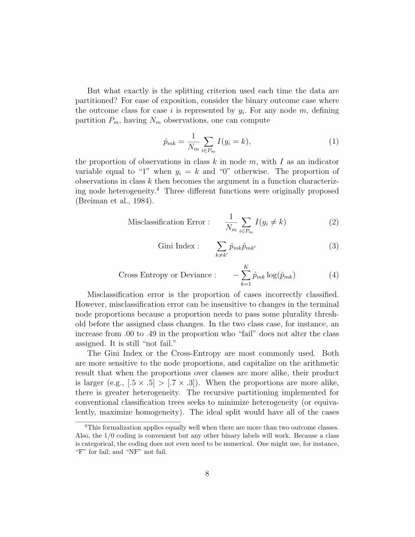
But what exactly is the splitting criterion used each time the data arepartitioned? For ease of exposition, consider the binary outcome case wherethe outcome class for case i is represented by yi. For any node m, definingpartition Pm, having Nm observations, one can compute

pmk =1

Nm

X

i2Pm

I(yi = k), (1)

the proportion of observations in class k in node m, with I as an indicatorvariable equal to “1” when yi = k and “0” otherwise. The proportion ofobservations in class k then becomes the argument in a function characteriz-ing node heterogeneity.4 Three di↵erent functions were originally proposed(Breiman et al., 1984).

Misclassification Error :1

Nm

X

i2Pm

I(yi 6= k) (2)

Gini Index :X

k 6=k0pmkpmk0 (3)

Cross Entropy or Deviance : �KX

k=1

pmk log(pmk) (4)

Misclassification error is the proportion of cases incorrectly classified.However, misclassification error can be insensitive to changes in the terminalnode proportions because a proportion needs to pass some plurality thresh-old before the assigned class changes. In the two class case, for instance, anincrease from .00 to .49 in the proportion who “fail” does not alter the classassigned. It is still “not fail.”

The Gini Index or the Cross-Entropy are most commonly used. Bothare more sensitive to the node proportions, and capitalize on the arithmeticresult that when the proportions over classes are more alike, their productis larger (e.g., [.5 ⇥ .5] > [.7 ⇥ .3]). When the proportions are more alike,there is greater heterogeneity. The recursive partitioning implemented forconventional classification trees seeks to minimize heterogeneity (or equiva-lently, maximize homogeneity). The ideal split would have all of the cases

4This formalization applies equally well when there are more than two outcome classes.Also, the 1/0 coding is convenient but any other binary labels will work. Because a classis categorical, the coding does not even need to be numerical. One might use, for instance,“F” for fail; and “NF” not fail.

8

with outcome class “1” in one node and all the cases with outcome class “0”in the other node. In our application to follow, we use the Gini Index wheneach partition is constructed.

3.2 Asymmetric Costs and Tuning

In practice, using a simple majority vote is unsatisfactory because false pos-itives and false negatives are treated as if they have the same costs; theirrelative costs are 1 to 1. Symmetric costs are the default in most software sothat if the arguments in the loss function are ignored, symmetric costs arenecessarily implemented. The California Static Risk Assessment Instrument,for instance, implicitly adopts the default of equal costs with no apparent ra-tionale (Turner, et al., 2009).

When symmetric costs are inconsistent with stakeholder preferences, thevotes in each terminal node can be weighted to take asymmetric relative costsinto account. For our later illustrative analysis, we make false negatives 5times more costly than false positives. Thus, failing to identify a high riskindividual is five times more costly than incorrectly labeling an individual ashigh risk.5 This weighting is broadly consistent with work we have done inthe past (Berk, 2012).6

However, more than the final vote should be altered (Hastie et al., 2009:310-311). The entire partitioning procedure should respond to di↵erentialcosts, and we proceed in this fashion below. In other words, the profilesthemselves are altered to account for the relative cost of false negatives tofalse positives. Hence, the entire classification tree is tuned to the 5 to 1 costratio. This can be accomplished by either altering the prior distribution ofthe outcome or by explicitly introducing a loss matrix into the classificationtree algorithm. We generally favor the latter because the relative costs areexplicitly represented.

Consider a K ⇥K loss matrix W. For simplicity, and with no important

5There is nothing special about the 5 to 1 cost ratio, and for the methodological issuesraised in the paper, most any reasonable cost ratio would su�ce. The cost ratio just couldnot be so extreme that the same class is assigned to essentially all cases. In that instance,the role of either false positives or false negatives would be obscured.

6Cost ratios have ranged from 20 to 1 to 3 to 1. The relative costs of false negatives aremore dear. Anectotally, we have found that criminal justive o�cials and representativefrom a variety of citizen’s groups broadly agree that at least for crimes of violence, falsenegatives are substantially more costly than false positives.

9

loss of generality, suppose that K = 2. The response outcomes are “fail” or“not fail.” When the forecasting procedure misses a failure, one has a falsenegative. When the forecasting procedure incorrectly identifies a failure, onehas a false positive. Then W is

"0 Rfn

Rfp 0

#

where the entries along the main diagonal are zero, and the o↵-diagonalelements contain the relative costs of false positives (i.e., Rfp) and false neg-atives (i.e., Rfn). The units do not matter. What matters is the ratio of thetwo. For example, Rfn could be 10, and Rfp could be 1. False negatives are10 times more costly than false positives. Put another way, 10 false positiveshave the same cost as 1 false negative.

Asymmetric costs, introduced so that the forecasts properly respond tostakeholder preferences, can a↵ect not just the recursive partitioning and theclasses assigned to terminal nodes, but evaluations of forecasting performanceas well. Standard evaluation tools such as the ROC curve take the forecastingoutput as is. If that output is based on equal costs, so is the ROC. If thecosts are not equal, performance measured by the ROC does not capturewhat decision-makers want (Hastie et al., 2009: Section 9.2.5). For example,risk forecasts that score well by the ROC may implicitly give too little weightto false positives. This may inadvertently increase prison populations anddiminish public confidence in the sentencing process.

Finally, for our illustrative analysis we chose tuning parameter valuesthat can help improve stability. The intent was to prevent the partitioningfrom proceeding too far; smaller trees tend to be more stable. Precisely howthis is done will depend on the software used. We applied rpart in R withwhich the number of terminal nodes can be controlled directly. One happyconsequence of smaller trees is that they can be easier to interpret.

3.3 Stability Analysis

Working with large data sets and smaller trees is unlikely to fully eliminatepotential instability. Had the data been even slightly di↵erent, it is possiblethat the splits chosen could have di↵ered substantially, leading to a new setof terminal nodes and perhaps new forecasts.

To consider how successful our strategy actually was, we explicitly ex-plored prediction instability. We generated a substantial number of boot-

10

strap samples, drawing from the training data with replacement. For eachsample, a classification tree was grown using tuning parameters at their pre-viously determined values. The classifications from each tree were stored.Cross tabulations were then undertaken for all possible pairs of trees. Fromeach cross tabulation, the proportion of times the classifications were thesame was computed. A very instructive analysis of tree stability followed,and some important refinements of the forecasts were implemented. Our ap-proach draws heavily on the work of Kuhnert and Mengersen (2003). Detailsare provided below.

In this context, it is important to appreciate that di↵erent tree structuresimply di↵erent substantive interpretations, and it is the structures that canbe especially unstable. Predictions derived from terminal nodes are typicallymore robust because all that matters is the forecasted class. Many di↵erenttree structures can lead to the same forecast for a given case. For example,if males under 21 are at high risk, it does not matter for forecasting whethergender defines the first partition and age the second or whether that orderis reversed. But it does matter if the variable used in the first partition istaken to be more important. It will also not matter if an age of 20 is choseninstead of 21 as long as 20 year olds and 21 year olds are assigned the sameclass as before through the impact of other predictors.

4 Data

The data used for the illustrative analysis includes individuals on probationin Philadelphia between 2002 and 2005. There are 48,923 observations witheach observation representing a case. An individual can appear in the datamore than once as di↵erent cases. Because sentencing decisions are madeon a case basis, using cases as the unit of analysis is consistent with theneeds of decision makers and how one might understand the social processesresponsible for the data. In fact, repeat o↵enders are not unusual, even overrelatively short time intervals, but decisions are made case by case. In short,the case/individual distinction has no important implications for forecastingprocedures we use, but there are some related issues for the stability analysisthat will be addressed later.

A random subset of the data were used as training data. These were thedata employed to construct the forecasting procedure. The remaining dataserved as test data from which honest assessments of forecasting accuracy

11

could be obtained. Having both training data and test data is consistenthonest performance assessments and with recommended practice (Hastie etal., 2009: Chapter 7).

4.1 Variables

Drawing on prior discussions with local stakeholders, the response variable forthe analysis is whether an individual once placed on probation was arrestedwithin two years for a violent crime: murder, attempted murder, manslaugh-ter, robbery, assault, kidnapping, rape, and arson. These are “failures.” Ofthe 48,923 cases, 6,284 cases “fail.” Thankfully, failures are relatively rare.Roughly 15% of all cases fail. All other outcome are treated as the absenceof “failure.”

Stakeholder rationale was this: a key consideration after most felony con-victions is whether to incarcerate. That decision should be informed at leastin part by a forecast of “future dangerousness.” Presumably, judges wouldbe less inclined to release an individual on probation if they are projected tocommit a violent crime.

There are, of course, other behavioral outcomes that could in principlebe predicted (Berk, 2012). One example is whether an individual is arrestedfor a murder (Berk et al., 2009). Another example is whether an individualis arrested for any felony. Yet another example allows for three outcomeclasses: an arrest for a violent crime, an arrest for a crime that is not violent,and no arrest for any felony. A similar three-class outcome has proved to beuseful for supervisory decisions of individuals on probation or parole (Barneset al., 2010).

The usual collection of covariates was available as potential predictors.They can be grouped as follows:

• Demographic Information: gender, date of birth

• Juvenile Priors: total number of priors, number of sex o↵ense priors,number of drug priors, etc.

• Adult Priors: total number of priors, number of sex o↵ense priors,number of murder priors, etc.

• Criminal Record Information: prior number of days in jail, numberof prior probation sentences, bail types, age at earliest prior, etc.

12

Race and ethnicity were excluded in deference to stakeholder sensitivi-ties. Predictors that should be excluded on other than statistical groundscan raise subtle technical issues because individual, neighborhood, and be-havioral attributes can be strongly related. In addition, because o↵enderstend to victimize individuals who share their “demographics,” controversialpredictors may be just those needed to help protect the most likely victims.We have discussed these matters in some detail elsewhere (Berk, 2009).

To further complicate matters, the set of predictors was not limited tothe covariates specified. A very important feature of classification trees isthat step functions and high order interaction e↵ects are automatically con-structed as needed. In e↵ect, a large number of empirically derived basisfunctions can be empirically determined. For example, young males fromhigh crime neighborhoods may be projected as high risk. The three con-stituent covariates (age, gender, and neighborhood) are combined as a three-way interaction that may serve as a surrogate for gang membership, which isnot directly measured. Age may serve as a splitting variable several times sothat a nonlinear function is approximated in several steps. In short, the set ofpotential predictors can far exceed the set of explicit predictors in ways thatare not likely be apparent. We refer interested readers to a more thoroughtreatment that is beyond the scope of this paper (Berk, 2012).

5 Random Forest Results

As a benchmark, we first employed random forests to the data. No othermachine learning procedure seems to perform any better for criminal jus-tice behavioral forecasting, although Bayesian additive regression trees andstochastic gradient boosting often forecast about as well (Berk, 2012). Anexposition of random forests is beyond the scope of this paper, and accessi-ble expositions are easily found (Berk, 2008b: chapter 5; Hastie et al., 2009:chapter 15).

Table 1 shows the confusion table that results. The confusion table is across-tabulation of the actual outcome and the forecasted outcome, and forrandom forests, these are real forecasts using data not employed to build theforecasting procedure.7

7In this context, a random forest is an ensemble of classification trees that di↵er fromone another by user-controlled chance processes. In one such process, when each tree isgrown, a random sample of observations is “held out” and serves as test data for that tree.

13

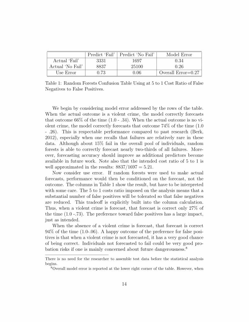
Predict ‘Fail’ Predict ‘No Fail’ Model ErrorActual ‘Fail’ 3331 1697 0.34

Actual ‘No Fail’ 8837 25100 0.26Use Error 0.73 0.06 Overall Error=0.27

Table 1: Random Forests Confusion Table Using at 5 to 1 Cost Ratio of FalseNegatives to False Positives.

We begin by considering model error addressed by the rows of the table.When the actual outcome is a violent crime, the model correctly forecaststhat outcome 66% of the time (1.0 - .34). When the actual outcome is no vi-olent crime, the model correctly forecasts that outcome 74% of the time (1.0- .26). This is respectable performance compared to past research (Berk,2012), especially when one recalls that failures are relatively rare in thesedata. Although about 15% fail in the overall pool of individuals, randomforests is able to correctly forecast nearly two-thirds of all failures. More-over, forecasting accuracy should improve as additional predictors becomeavailable in future work. Note also that the intended cost ratio of 5 to 1 iswell approximated in the results: 8837/1697 = 5.21.

Now consider use error. If random forests were used to make actualforecasts, performance would then be conditioned on the forecast, not theoutcome. The columns in Table 1 show the result, but have to be interpretedwith some care. The 5 to 1 costs ratio imposed on the analysis means that asubstantial number of false positives will be tolerated so that false negativesare reduced. This tradeo↵ is explicitly built into the column calculation.Thus, when a violent crime is forecast, that forecast is correct only 27% ofthe time (1.0 -.73). The preference toward false positives has a large impact,just as intended.

When the absence of a violent crime is forecast, that forecast is correct94% of the time (1.0-.06). A happy outcome of the preference for false posi-tives is that when a violent crime is not forecasted, it has a very good chanceof being correct. Individuals not forecasted to fail could be very good pro-bation risks if one is mainly concerned about future dangerousness.8

There is no need for the researcher to assemble test data before the statistical analysisbegins.

8Overall model error is reported at the lower right corner of the table. However, when

14

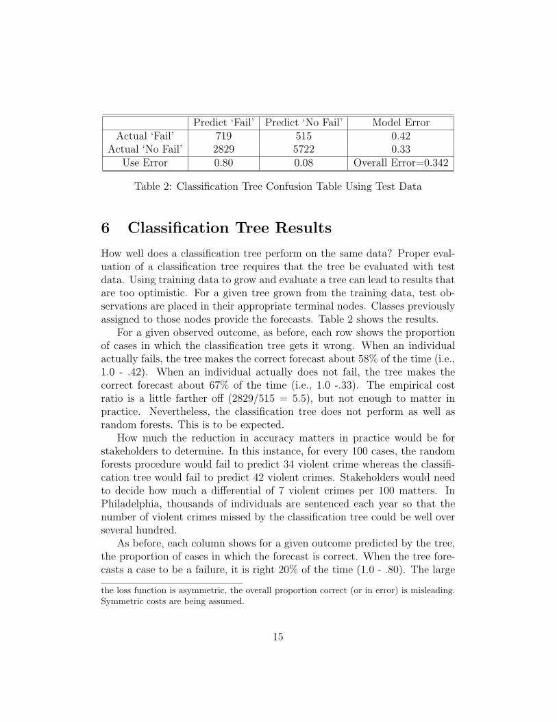
Predict ‘Fail’ Predict ‘No Fail’ Model ErrorActual ‘Fail’ 719 515 0.42

Actual ‘No Fail’ 2829 5722 0.33Use Error 0.80 0.08 Overall Error=0.342

Table 2: Classification Tree Confusion Table Using Test Data

6 Classification Tree Results

How well does a classification tree perform on the same data? Proper eval-uation of a classification tree requires that the tree be evaluated with testdata. Using training data to grow and evaluate a tree can lead to results thatare too optimistic. For a given tree grown from the training data, test ob-servations are placed in their appropriate terminal nodes. Classes previouslyassigned to those nodes provide the forecasts. Table 2 shows the results.

For a given observed outcome, as before, each row shows the proportionof cases in which the classification tree gets it wrong. When an individualactually fails, the tree makes the correct forecast about 58% of the time (i.e.,1.0 - .42). When an individual actually does not fail, the tree makes thecorrect forecast about 67% of the time (i.e., 1.0 -.33). The empirical costratio is a little farther o↵ (2829/515 = 5.5), but not enough to matter inpractice. Nevertheless, the classification tree does not perform as well asrandom forests. This is to be expected.

How much the reduction in accuracy matters in practice would be forstakeholders to determine. In this instance, for every 100 cases, the randomforests procedure would fail to predict 34 violent crime whereas the classifi-cation tree would fail to predict 42 violent crimes. Stakeholders would needto decide how much a di↵erential of 7 violent crimes per 100 matters. InPhiladelphia, thousands of individuals are sentenced each year so that thenumber of violent crimes missed by the classification tree could be well overseveral hundred.

As before, each column shows for a given outcome predicted by the tree,the proportion of cases in which the forecast is correct. When the tree fore-casts a case to be a failure, it is right 20% of the time (1.0 - .80). The large

the loss function is asymmetric, the overall proportion correct (or in error) is misleading.Symmetric costs are being assumed.

15

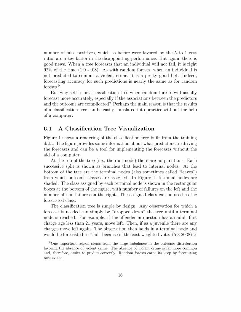
number of false positives, which as before were favored by the 5 to 1 costratio, are a key factor in the disappointing performance. But again, there isgood news. When a tree forecasts that an individual will not fail, it is right92% of the time (1.0 - .08). As with random forests, when an individual isnot predicted to commit a violent crime, it is a pretty good bet. Indeed,forecasting accuracy for such predictions is nearly the same as for randomforests.9

But why settle for a classification tree when random forests will usuallyforecast more accurately, especially if the associations between the predictorsand the outcome are complicated? Perhaps the main reason is that the resultsof a classification tree can be easily translated into practice without the helpof a computer.

6.1 A Classification Tree Visualization

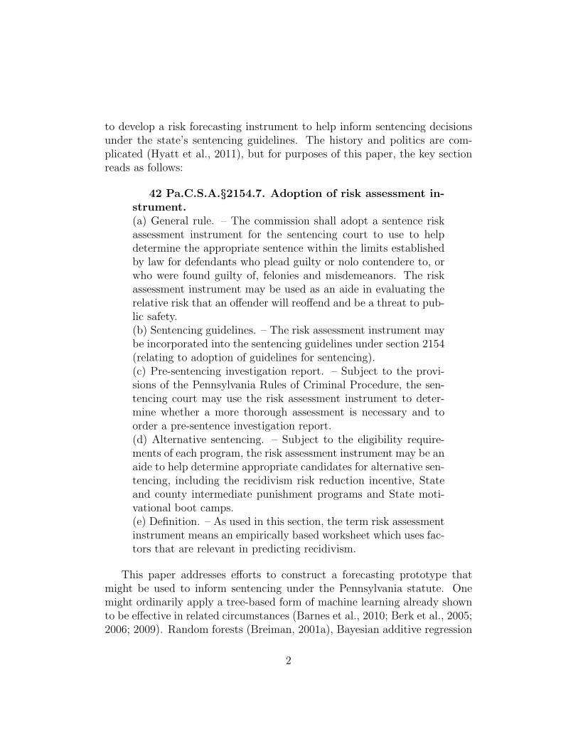
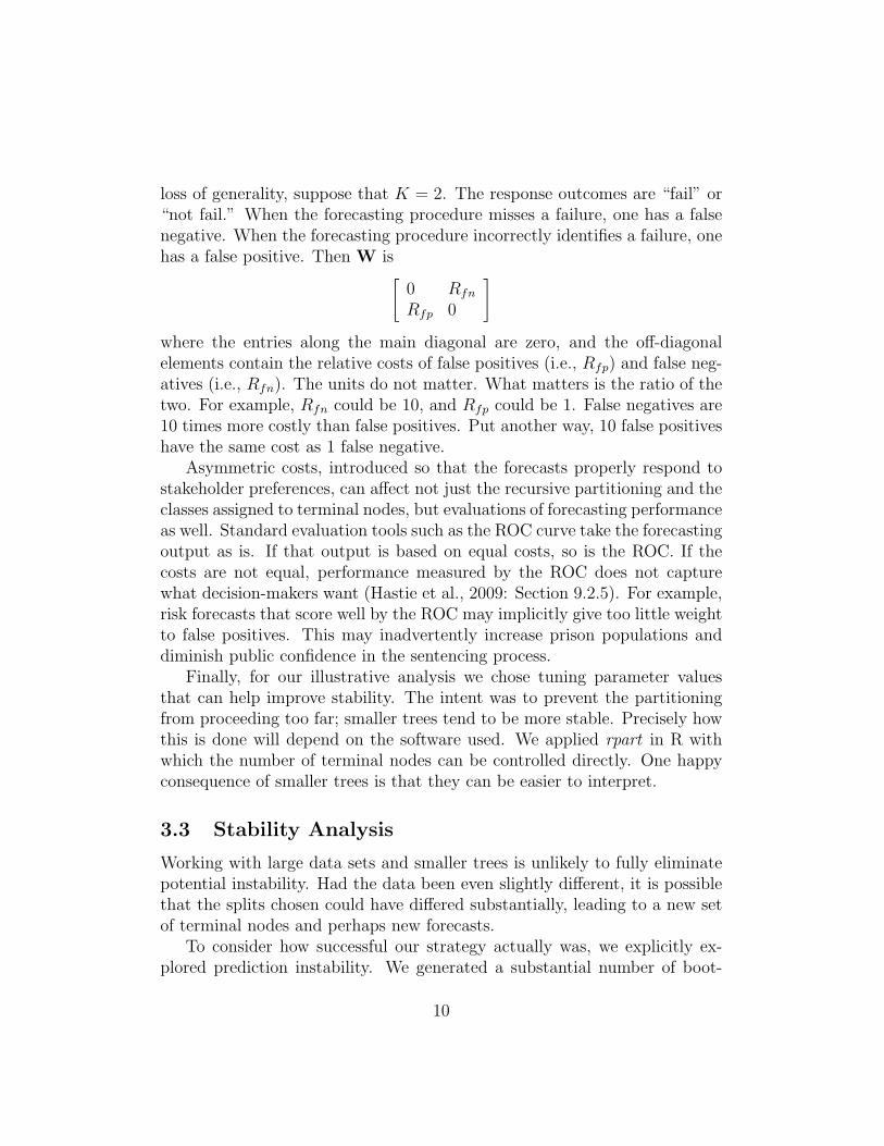
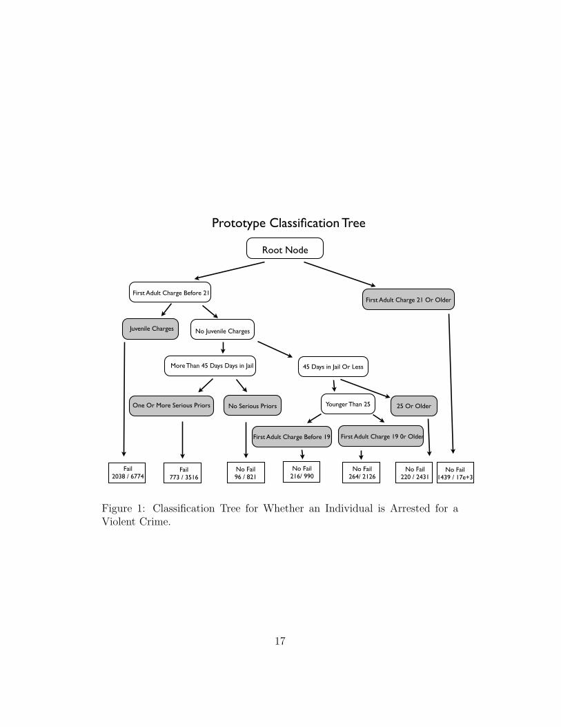
Figure 1 shows a rendering of the classification tree built from the trainingdata. The figure provides some information about what predictors are drivingthe forecasts and can be a tool for implementing the forecasts without theaid of a computer.

At the top of the tree (i.e., the root node) there are no partitions. Eachsuccessive split is shown as branches that lead to internal nodes. At thebottom of the tree are the terminal nodes (also sometimes called “leaves”)from which outcome classes are assigned. In Figure 1, terminal nodes areshaded. The class assigned by each terminal node is shown in the rectangularboxes at the bottom of the figure, with number of failures on the left and thenumber of non-failures on the right. The assigned class can be used as theforecasted class.

The classification tree is simple by design. Any observation for which aforecast is needed can simply be “dropped down” the tree until a terminalnode is reached. For example, if the o↵ender in question has an adult firstcharge age less than 21 years, move left. Then, if as a juvenile there are anycharges move left again. The observation then lands in a terminal node andwould be forecasted to “fail” because of the cost-weighted vote: (5⇥2038) >

9One important reason stems from the large imbalance in the outcome distributionfavoring the absence of violent crime. The absence of violent crime is far more commonand, therefore, easier to predict correctly. Random forests earns its keep by forecastingrare events.

16

Prototype Classification Tree

Root Node

First Adult Charge Before 21First Adult Charge 21 Or Older

Juvenile Charges

Fail2038 / 6774

More Than 45 Days Days in Jail

No Juvenile Charges

45 Days in Jail Or Less

One Or More Serious Priors No Serious Priors

No Fail96 / 821

Fail773 / 3516

Younger Than 25 25 Or Older

No Fail1439 / 17e+3

First Adult Charge Before 19 First Adult Charge 19 0r Older

No Fail216/ 990

No Fail264/ 2126

No Fail220 / 2431

Figure 1: Classification Tree for Whether an Individual is Arrested for aViolent Crime.

17

6774. If the second split sends a case to the right, there are additionalpartitions before one of several terminal nodes is reached.

All observations in need of a forecast can be treated in a similar fashionand will fall into one of the terminal nodes. As a result, the tree structurecreates a straightforward set of selection criteria that can aid in sentencingdecisions. One just follows that path appropriate for a given o↵ender to itsterminal node for which the predicted outcome is provided. In short, theclassification tree results can be used in a paper-and-pencil fashion.

The structure of the tree can also provide subject-matter insights. Forexample, the terminal node on the far right contains all individuals whosefirst criminal charge occurred after the age of 21. They are the best risks. Forthose arrested and charged before they were 21, the class assigned dependsupon interactions with other variables. For example, one relatively high riskgroup is composed of individuals whose first adult criminal charge was beforethe age of 21, who had a criminal charge as a juvenile, who spent at least 46days in jail previously and who had at least one serious charge as an adult. Inlinear model terms, this is a high order interaction e↵ect that would probablynot have been specified a priori or discovered with conventional regressiondiagnostics. At best, each constituent of the interaction would have beenincluded as a main e↵ect.

It is important to stress, however, that forecasting is the goal. Even ifthere are substantive insights in the tree structure, a classification tree is nota causal model. At best, there can be provocative associations.

6.2 Stability Analysis

There is a relatively small literature on uncertainty in classification trees, andit is segmented into somewhat di↵erent estimation problems and applications.Holmes (2003) provides an excellent review for phylogenetic applications thathas broader implications. A very di↵erent tradition can be found in computerscience (Toth, 2008). The work of Kuhnert and Mengersen (2003) seems mostrelevant to a sentencing setting.

Kunhnert and Mengersen consider several kinds of reliability questionsbut for us, the following question seems most germaine. For a given classifi-cation tree, how reliable are terminal node classifications over realizations ofthe data? Here are the steps.

1. Generate B bootstrap “test” samples, sampling with replacement from

18

the training data.

2. Using the original classification tree, drop each test sample down thetree and determine the class label to be attached to each terminal nodeusing the Bayes classifier (i.e., the class assigned is the class with themost cases).

3. Compute the proportion of times the class assigned to the terminalnodes is the same as the class assigned with the original data.

All of the uncertainty is driven by sampling variation in the test samples.There is no uncertainty in the model itself. Moreover, stability is defined overterminal nodes, not the cases that fall within them. So a node containing10 cases is treated the same as a node containing 100 cases even though achange in how the node is labeled a↵ects 10 times more cases for the secondnode.

We find this formulation insu�ciently responsive to our application. First,we view our classification tree as illustrative, not definitive. It could wellchange with new data from sampling variation alone. It is important, there-fore, to capture model uncertainty. Second, judges sentence cases. It is thestability of case classifications that matters. Stability should be representedat the level of cases, not the level of terminal nodes.

As a result, we implement the following procedure.

1. We generated 50 “new” samples with replacement from the trainingdata using the same number of observations as in the training data.

2. For each new sample, a classification tree was grown as before with thesame values for the tuning parameters. The result was a total of 50trees.10

3. The classifications from each tree were stored.

4. For each possible pair of the 50 trees (i.e., 1225), we computed theproportion of times the classifications were the same.11

10We used the same tuning parameter values so that the trees were comparable. Wewere trying to isolate the impact of new data for a tree of a given complexity. Had wealtered the tuning parameter values, changes in how cases were classified could result fromeither the new data or di↵ering tuning parameters. The cost ratio was also unchanged.

11One reason by Kuhnert and Mengersen suggest additional measures of stability is that

19

6.2.1 Some Technical Issues

Recall that the unit of analysis is the case, not the individual. As a result,some individuals are included in the data more than once. Substantively,this is not a problem because judges make sentencing decisions for cases asthey come up and repeat o↵enders, even within short time intervals, are notunusual.

If there are problems, they technical. First, our stability analysis appro-priately sampled cases independently with replacement. If sampling were notwith replacement, each of the samples would necessarily be identical to theoriginal data and to each other. However, the data can be seen as a randomrealization of the social processes that generate cases in need of sentences,for which there is, in e↵ect, simple random sampling of cases. Because a casecannot be sentenced more than once, the sampling is without replacement.

Second, sampling without replacement also is an imperfect formalizationfor how the data were perhaps generated. It is possible that once a givenindividual has been selected, there is an increased probability that that in-dividual will be selected again. Perhaps criminal behavior becomes morelikely and/or the criminal justice system is primed to arrest and punish thatindividual. Alternatively, it is possible that the experience of being arrested,convicted, sentenced and sanctioned reduces the probability that an indi-vidual will be selected again because criminal behavior is deterred. If thesanction involves e↵ective probation supervision, behavior may be changedfor the better. If the sanction involves incarceration, time on the streets (atleast in the short to medium term) is reduced.

The first problem implies that we may be underestimating instability, atleast a bit. Our e↵ective sample size is smaller than our nominal samplesize. The second problem could lead to some underestimation or overesti-mation of instability depending on how the two competing forces balance fora large number of cases. We will revisit these issues after some results aresummarized.

they apparently do not find su�ciently strong justification for using a Bayes classifier. Inour context, where the relative costs of false negatives and false positives are elicited fromstakeholders, their concerns seem far less troubling.

20

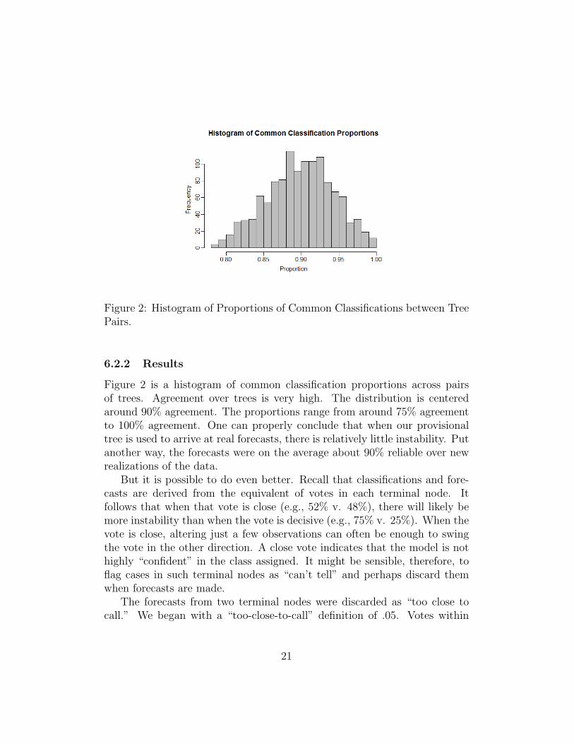
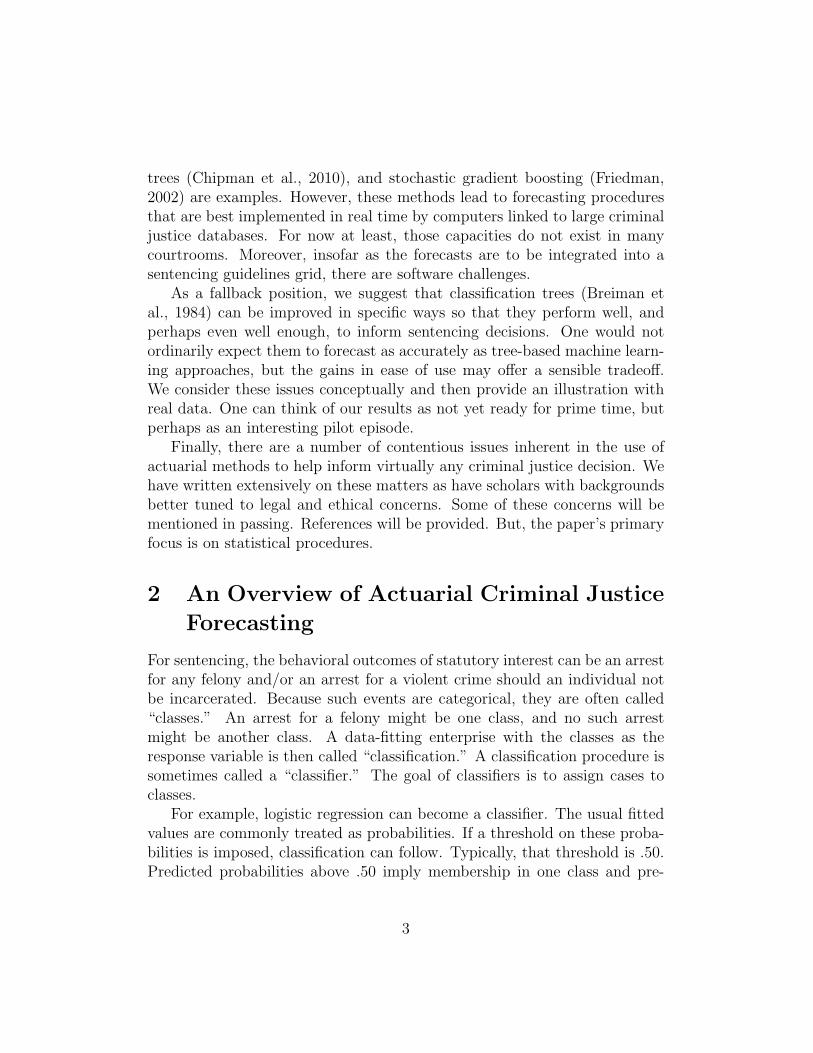
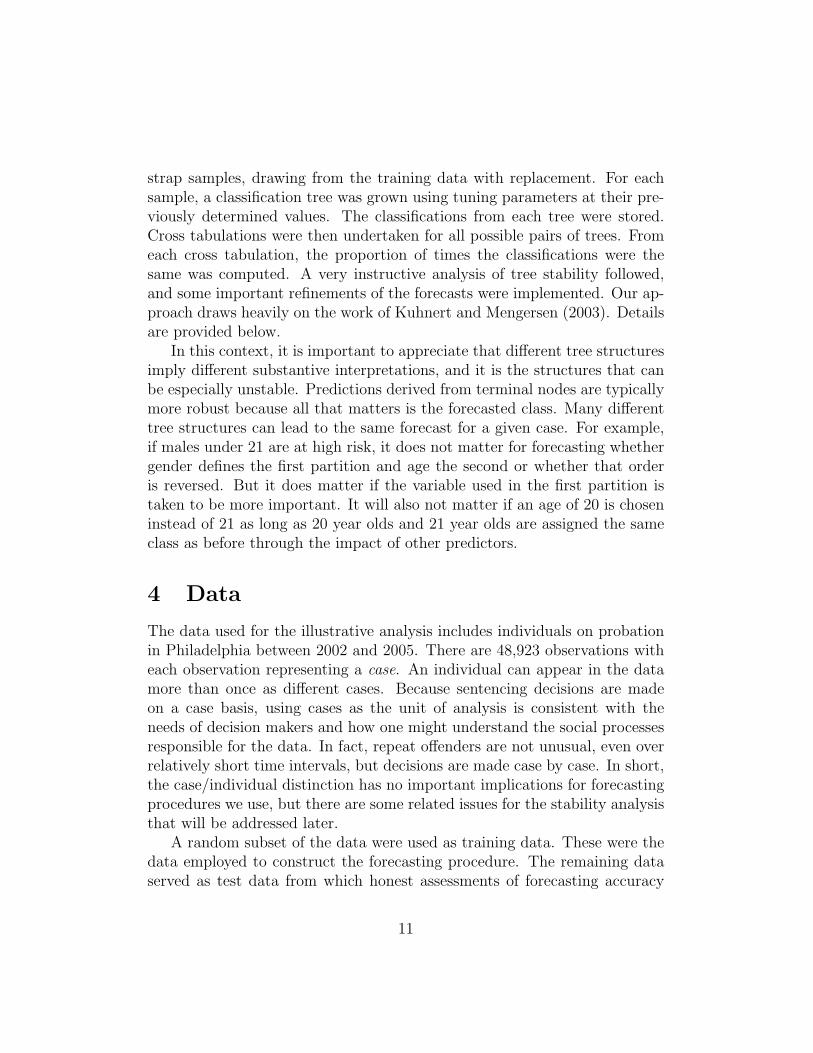
Figure 2: Histogram of Proportions of Common Classifications between TreePairs.

6.2.2 Results

Figure 2 is a histogram of common classification proportions across pairsof trees. Agreement over trees is very high. The distribution is centeredaround 90% agreement. The proportions range from around 75% agreementto 100% agreement. One can properly conclude that when our provisionaltree is used to arrive at real forecasts, there is relatively little instability. Putanother way, the forecasts were on the average about 90% reliable over newrealizations of the data.

But it is possible to do even better. Recall that classifications and fore-casts are derived from the equivalent of votes in each terminal node. Itfollows that when that vote is close (e.g., 52% v. 48%), there will likely bemore instability than when the vote is decisive (e.g., 75% v. 25%). When thevote is close, altering just a few observations can often be enough to swingthe vote in the other direction. A close vote indicates that the model is nothighly “confident” in the class assigned. It might be sensible, therefore, toflag cases in such terminal nodes as “can’t tell” and perhaps discard themwhen forecasts are made.

The forecasts from two terminal nodes were discarded as “too close tocall.” We began with a “too-close-to-call” definition of .05. Votes within

21

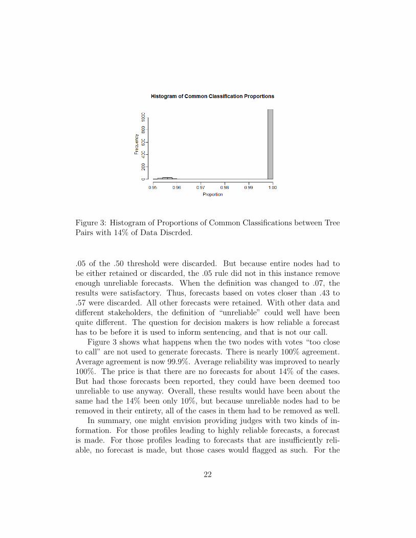
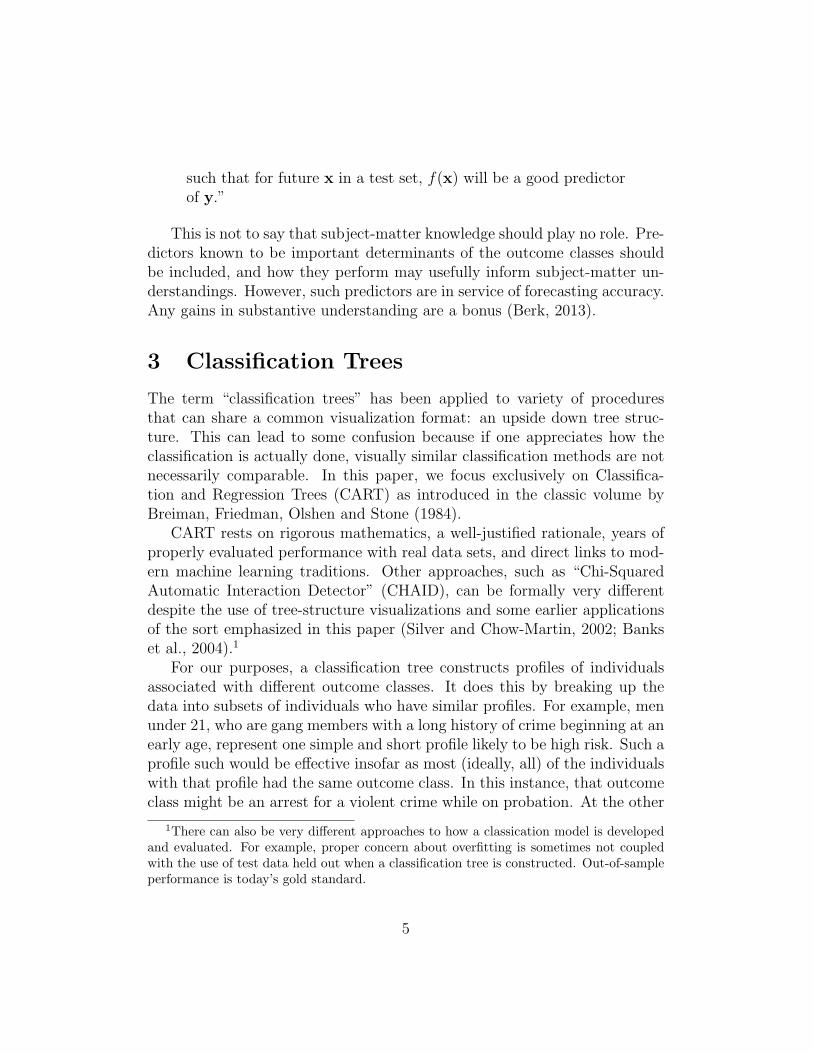
Figure 3: Histogram of Proportions of Common Classifications between TreePairs with 14% of Data Discrded.

.05 of the .50 threshold were discarded. But because entire nodes had tobe either retained or discarded, the .05 rule did not in this instance removeenough unreliable forecasts. When the definition was changed to .07, theresults were satisfactory. Thus, forecasts based on votes closer than .43 to.57 were discarded. All other forecasts were retained. With other data anddi↵erent stakeholders, the definition of “unreliable” could well have beenquite di↵erent. The question for decision makers is how reliable a forecasthas to be before it is used to inform sentencing, and that is not our call.

Figure 3 shows what happens when the two nodes with votes “too closeto call” are not used to generate forecasts. There is nearly 100% agreement.Average agreement is now 99.9%. Average reliability was improved to nearly100%. The price is that there are no forecasts for about 14% of the cases.But had those forecasts been reported, they could have been deemed toounreliable to use anyway. Overall, these results would have been about thesame had the 14% been only 10%, but because unreliable nodes had to beremoved in their entirety, all of the cases in them had to be removed as well.

In summary, one might envision providing judges with two kinds of in-formation. For those profiles leading to highly reliable forecasts, a forecastis made. For those profiles leading to forecasts that are insu�ciently reli-able, no forecast is made, but those cases would flagged as such. For the

22

second group, a proper inference is that one cannot decide from the availabledata and statistical procedures how the individual will perform.12 Therefore,sentences would be determined without quantitative forecasts of risk.

More broadly framed, our stability analysis addresses an important kindof uncertainty in the tree-based, quantitative forecasts. How likely is it thata di↵erent forecast would be made with new realizations for the data? Withour large sample and small classification tree, there is almost no instabilityuncertainty in the forecasts for about 85% of the cases. Instability uncer-tainty would likely be greater in other analyses with substantially smallersamples and/or substantially larger trees. Instability uncertainty would alsobe a↵ected by the strength of relationships between the predictors and theoutcome. As best we can tell, uncertainty in classification tree forecasts hasnot been addressed in this simple fashion before. We re-emphasize, how-ever, the our concern is with instability in forecasts, not instability in treestructure. The latter can be far more unstable than the former.

One could also imagine providing judges with the votes for each forecastso that the reliability of each forecast could be taken into account. As apractical matter, we thought this was far too heavy a burden to place onthe sentencing process, especially because in our illustration at least, mostforecasts were highly reliable. But as a technical matter, that informationwould be available and easily accessed. An outline of the computer code usedfor the stability analysis is provided in the appendix.

7 Conclusions

The failure outcome for this population is relatively rare: about 15% of thecases fail through an arrest for a violent crime. Nevertheless, even a verysimple classification tree is able with test data to correctly identify about60% of those who fail. Of those who do not fail, about 67% are correctlyidentified.

Foresting accuracy depends especially heavily and directly on the 5 to1 cost ratio of false negatives to false positives. By design, this opens thedoor to a substantial number of false positives so that forecasts of failureare correct only about 21% of the time. But another consequence is that

12Even using the same data, it is likely that a machine learning procedure would dobetter. Recall, however, that in this paper we are assuming that machine learning is nota practical option.

23

forecasting accuracy for individual who do not fail is over 90%. That is, ifa forecast of not failing is made, it is quite likely to be correct. If this kindof information were to be used in sentencing, there would a large pool ofconvicted o↵enders who might be good probation risks. But one must beclear that by “good” risks, we mean with respect to a violent crime only.

It might be more useful in the future to redefine the response, as we havein other applications, to measure three outcomes: an arrest for a violentcrime, an arrest for a crime that is not violent, and no arrest at all. Orperhaps some other three-way break would be more appropriate. The pointis that by using three outcome classes instead of two, less ham-fisted distinc-tions can be made. An individual would be forecasted into one of the threeoutcomes, not one of two. The procedures discussed above would still apply,although the algorithmic output would be a bit more complicated.

We found that the forecasts are quite reliable. Instability does not seemto be a problem for about 85% of the cases. The small tree grown from a largesample no doubt helps a lot. If one discards the relatively small number ofcases whose forecasts are deemed unreliable, instability virtually disappears.More generally, the stability analysis provides information on the uncertaintyin tree-based forecasts that judges might find helpful.

Whatever one thinks of the results, it is possible to do substantially better.A high priority is obtaining better data from an appropriate population ofo↵enders. That process has begun. Finally, cost ratios of false negatives tofalse positives should be obtained from stakeholders. Indeed, several di↵erentcost ratios might be relevant. These alone could significantly change theresults.

Appendix — Outline of Software for StabilityAssessments

The steps that follow summarize the R code used to discard unreliable fore-casts.

1. Construct a classification tree using a loss-matrix with the desired costs.

2. For each case, find the terminal node where it was classified.

3. Create a table that shows for each terminal node, how many observa-tions in that node were labelled “Fail” vs. “No Fail.”

24

4. To understand how close the vote in each node was, re-weight the“Fails” in each by their weight as if they were false negatives (e.g.,assign a cost of 5.0 to each failure). This now allows one to check themajority vote (using weighted fails) to see which classification won.

5. Let F be the weighted sum of all the ”Fails” (e.g., 400 fails X 5.0 cost= 2000) and NF be total number of non-failures, each with a weightof 1.0). Let p = F/(F + NF ), the proportion of the weighted totalnumber of votes that are “Fail” in a given terminal node. This can bedone symmetrically with 1� p as well.

6. Set a desired margin. Check if the absolute value of (p� .5) is too closeto call. How close is too close will require some trial and error.

7. Store which nodes are too close and which are not. Use the outputfrom the tree with the additional label that some nodes are now tooclose too call.

8. One can exclude these too-close observations and run a cross-checkagainst the bootstrapped trees to see how the stability improves.

References

Banks, S., Robbins, P.C., Silver, E., Vesselinov, R., Steadman, H.J., Mon-ahan, J., Mulvey, E.P., Applebaum, P.S., Grisso, RT., & Roth, L.H.(2004) “A Multiple-Models Approach to Violence Risk Assessment AmongPeople with Mental Disorder.” Criminal Justice and Behavior 31: 324–340.

Barnes, G.C., Ahlman, L., Gill, C., Sherman, L.W., Kurtz, E., & Malves-tuto, R. (2010) “Low Intensity Community Supervision for Low-RiskO↵enders: A Randomized, Controlled Trial.” Journal of ExperimentalCriminology 6: 159-189.

Berk, R. A. (2008a) “Forecasting Methods in Crime and Justice.” In J.Hagan, K. L. Schepple, & T. R. Tyler (eds.) Annual Review of Lawand Social Science 4 (173–192). Palo Alto: Annual Reviews.

Berk., R. A. (2008b) Statistical Learning from a Regression Perspective.New York: Springer.

25

Berk., R. A.(2009) “The Role of Race in Forecasts of Violent Crime.” Raceand Social Problems 1(4): 231–242.

Berk, R.A. (2011) “Asymmetric Loss Functions for Forecasting in CriminalJustice Settings.” Journal of Quantitative Criminology 27: 107-123,2011.

Berk, R. A. (2012) Criminal Justice Forecasts of Risk: A Machine LearningApproach. New York: Springer.

Berk, R.A. (2103, forthcoming) “Algorithmic Criminology.” Security Infor-matics.

Berk, R. A., Brown, L., & Zhao, L. (2010) “Statistical Inference After ModelSelection.” Journal of Quantitative Criminology, 26(2): 217–236.

Berk. R. A., Kriegler, B., & Baek, J-H. (2006) “Forecasting Dangerous In-mate Misconduct: An Application of Ensemble Statistical Procedures.”Journal of Quantitative Criminology 22(2) 135–145.

Berk, R. A., Sorenson, S. B., & He, Y. (2005) “Developing a Practical Fore-casting Screener for Domestic Violence Incidents.” Evaluation Review29(4): 358–382.

Berk, R. A., Sherman, L., Barnes, G., Kurtz, E., & Ahlman, L. (2009)“Forecasting Murder within a Population of Probationers and Parolees:A High Stakes Application of Statistical Learning.” Journal of theRoyal Statistics Society — Series A 172 (part I): 191–211.

Borden, H. G. (1928) “Factors Predicting Parole Success.” Journal of theAmerican Institute of Criminal Law and Criminology 19: 328–336.

Burgess, E. M. (1928) “Factors Determining Success or Failure on Parole.”In A. A. Bruce, A. J. Harno, E. .W Burgess, & E. W., Landesco (eds.)The Working of the Indeterminate Sentence Law and the Parole Systemin Illinois (pp. 205–249). Springfield, Illinois, State Board of Parole.

Bushway, S. (2011) Albany Law Review 74 (3).

Breiman, L. (2001a) “Random Forests.” Machine Learning 45: 5–32.

26

Breiman, L. (2001b) “Statistical Modeling: Two Cultures.” (with discus-sion). Statistical Science 16: 199–231.

Breiman, L., Friedman, J.H., Olshen, R.A., & Stone, C.J. (1984) Classifi-cation and Regression Trees. Monterey, CA: Wadsworth Press.

Casey, P. M., Warren, R. K., & Elek, J. K. (2011) “Using O↵ender Riskand Needs Assessment Information at Sentencing: Guidance from aNational Working Group.” National Center for State Courts,www.ncsconline.org/.

Chipman, H. A., George, E. I., & McCulloch, R. E. (2010) “BART: BayesianAdditive Regression Trees.” Annals of Applied Statistics 4(1): 266–298.

Farrington, D. P. & Tarling, R. (2003) Prediction in Criminology. Albany:SUNY Press.

Feeley, M., & Simon, J. (1994). “Actuarial Justice: The Emerging NewCriminal Law.” In D. Nelken (ed.), The Futures of Criminology (pp.173201). London: Sage Publications.

Friedman, J. H. (2002)“Stochastic Gradient Boosting.” ComputationalStatistics and Data Analysis 38: 367–378.

Gottfredson, S. D., & Moriarty, L. J. (2006) “Statistical Risk Assessment:Old Problems and New Applications.” Crime & Delinquency52(1):178–200.

Harcourt, B.W. (2007) Against Prediction: Profiling, Policing, and Punish-ing in an Actuarial Age. Chicago, University of Chicago Press.

Hastie, R., & Dawes, R. M. (2001) Rational Choice in an Uncertain World.Thousand Oaks: Sage Publications.

Hastie, T., Tibshirani, R., & Friedman, J. (2009) The Elements of StatisticalLearning. Second Edition. New York: Springer.

Holmes, S. (2003) “Bootstrapping Phylogenetic Trees: Theory and Meth-ods.” Statistical Science 18(2): 241-255.

27

Hyatt, J.M., Chanenson, L. & Bergstrom, M.H. (2011) “Reform in Motion:The Promise and Profiles of Incorporating Risk Assessments and Cost-Benefit Analysis into Pennsylvania Sentencing.” Duquesne Law Review49(4): 707–749.

Kleiman, M., Ostrom, B. J., & Cheeman, F. L. (2007) “Using Risk As-sessment to Inform Sentencing Decisions for Nonviolent O↵enders inVirginia.” Crime & Delinquency 53(1): 1–27.

Kuhnert, P.M., & Mengersen, K. (2003) “Reliability Measures for LocalNodes Assessment in Classification Trees.” Journal of Computationaland Graphical Statistics 12(2): 398–426.

Messinger, S.L., & Berk, R.A. (1987) “Dangerous People: A Review of theNAS Report on Career Criminals.” Criminology 25(3): 767–781

Monahan, J. (1981) Predicting Violent Behavior: An Assessment of ClinicalTechniques. Newbury Park: Sage Publications.

Monahan, J. (2006) “A Jurisprudence of Risk Assessment: ForecastingHarm Among Prisoners, Predators, and Patients.” Virginia Law Re-view 92: 391–435.

Monahan, J., & Solver, E. (2003) “Judicial Decision Thresholds for ViolenceRisk Management.” International Journal of Forensice Mental Health2(1): 1–6.

Oregon Youth Authority (2011) “OYA Recidivism Risk Assessment — Vi-olent Crime (ORRA-V): Modeling Risk to Recidivate with a ViolentCrime.” Oregon Youth Authority, Salem, OR.

Pew Center of the States, Public Safety Performance Project (2011) “Risk/NeedsAssessment 101: Science Reveals New Tools to Manage O↵enders.”The Pew Center of the States. www.pewcenteronthestates.org/publicsafety.

Silver, E., & Chow-Martin, L. (2002) “A Multiple Models Approach toAssessing Recidivism Risk: Implications for Judicial Decision Making.”Criminal Justice and Behavior 29: 538–569

Skeem, J. .L., & Monahan, J. (2011) “Current Directions in Violence RiskAssessment.” Current Directions in Psychological Science 21(1): 38–42.

28

Sorensen, J. R., & Pilgrim, R. L. (2000) “An Actuarial Risk Assessmentof Violence Posed by Capital Murder Defendants.” The Journal ofCriminal Law and Criminology 90: 1251–1270.

Toth, N. (2008) Handling Classification Uncertainty with Decision Treesin Biomedical Diagnostic Systems. Ph.D. Thesis, Department of Mea-surement and Information Systems, Budapest University of Technologyand Economics.

Turner, S., Hess, J., & Jannetta, J. (2009) Development of the CaliforniaRisk Assessment Instrument. Center for Evidence Based Corrections,The University of California, Irvine

29