foreign exchange value-at-risk with multiple currency exposure · foreign exchange value-at-risk...

Defence Research andDevelopment Canada

Recherche et developpementpour la defense Canada

Foreign exchange value-at-risk with multiple currency exposure

A multivariate and copula generalized autoregressive conditionalheteroskedasticity approach

David W. Maybury

Defence Research and Development Canada

Scientific ReportDRDC-RDDC-2014-R62November 2014

Foreign exchange value-at-risk with multiplecurrency exposureA multivariate and copula generalized autoregressive conditionalheteroskedasticity approach

David W. Maybury

Defence Research and Development CanadaScientific ReportDRDC-RDDC-2014-R62November 2014

c© Her Majesty the Queen in Right of Canada (Department of National Defence), 2014

c© Sa Majesté la Reine en droit du Canada (Ministère de la Défense nationale), 2014

Abstract

Large DND projects and acquisitions are exposed to more than one foreign currency at

the same time which complicates management’s foreign exchange risk assessments. We

extend the Centre for Operational Research and Analysis’ (CORA) in-house Generalized

Autoregressive Conditional Heteroskedasticity (GARCH) models to a full multivariate set-

ting. Our extensions involve two models types: multivariate GARCH and copula-GARCH.

We find that both models give qualitatively similar value-at-risk (VaR) estimates, and that

both models provide a much improved risk assessment relative to the current practice – cor-

recting VaR estimates on the order of 25% in cases in which multiple currency exposures

are of similar size. Using the USDCAD, the EURCAD, and the GBPCAD, we demon-

strate estimation techniques for each model. Finally, we show the strength of our improved

models through a 100-day VaR calculation.

DRDC-RDDC-2014-R62 i

Significance for defence and security

The Department of National Defence (DND) expends approximately 10% of its annual

budget in foreign currencies in support of equipment, acquisitions, and operations. The for-

eign currency transactions within DND’s budget expose the department to financial market

risk in the form of fluctuating exchange rates, placing additional risk mitigation pressures

on internal management. Given the Government of Canada’s planned military acquisitions

in the form of the CF-188 replacement and the renewal of the Royal Canadian Navy – both

of which will contain significant foreign content – exchange rate risk has quickly become

an important risk element for DND management to understand.

In this study, we extend our in-house financial risk models to help DND understand the

extent of risk mitigation that occurs naturally through exposure to more than one currency.

DND’s main foreign currency exposure involves the US dollar, the euro, and the British

pound sterling. To gauge the effect of adverse currency fluctuations on DND’s budgets and

planning, we require an understanding of the strength of natural diversification benefits

within value-at-risk (VaR) analyses. We examine two methods to attack this problem. Our

first approach uses multivariate correlation methods which extract time dependence and

persistence in correlations between exchange rate pairs. In our second approach, we build

dependency models between exchange rate pairs using copulas. Both modelling techniques

offer decision makers a deeper understanding of portfolio VaR – correcting the indepen-

dence assumed VaR estimate by 25% in cases in which multiple currency exposures are of

similar size.

ii DRDC-RDDC-2014-R62

Résumé

Dans ses grands projets et achats, le MDN doit souvent composer avec plusieurs devises

à la fois, ce qui complique son évaluation des risques. Nous avons amplifié des modèles

d’hétéroscédasticité conditionnelle autorégressive généralisée (GARCH) du Centre d’ana-

lyse et de recherche opérationnelle (CARO) de manière à y inclure toutes les variables

nécessaires. Nous avons, de fait, modifié deux types de modèle : le modèle GARCH à

variables multiples et le modèle GARCH à copules. Nous avons constaté que les deux mo-

dèles donnent des estimations de la valeur à risque (VaR) de qualités comparables et qu’ils

permettent d’effectuer une meilleure évaluation du risque qu’avec la méthode courante. On

obtient désormais des estimations de la VaR 25% plus exactes pour les cas où plusieurs

devises entrent en jeu. Au moyen des combinaisons USD-CAD, EUR-CAD et GBP-CAD,

nous avons démontré les techniques d’estimation des deux modèles. Enfin, nous avons dé-

montré la fiabilité de nos modèles améliorés au moyen d’un calcul de la VaR sur 100 jours.

DRDC-RDDC-2014-R62 iii

Importance pour la défense et la sécurité

Le ministère de la Défense nationale (MDN) dépense environ 10% de son budget annuel

en devises étrangères pour l’entretien de son équipement, ses achats et ses opérations. Ces

transactions en devises étrangères exposent le MDN à un risque financier lié aux varia-

tions du taux de change, et les responsables de la gestion interne se voient donc pressés

de trouver des stratégies d’atténuation. Comme le gouvernement du Canada prévoit faire

d’importantes acquisitions militaires, notamment pour remplacer le CF188 et renouveler la

Marine royale canadienne (deux projets dans lesquels il fera beaucoup affaire avec l’étran-

ger), le risque lié au taux de change est rapidement devenu un élément important que la

direction du MDN se doit de maîtriser.

Dans notre étude, nous avons amplifié nos modèles maison d’évaluation du risque finan-

cier dans le but d’aider le MDN à comprendre l’importance de l’atténuation des risques

lorsqu’on doit composer avec plus d’une devise. Les principales devises étrangères que le

MDN rencontre le plus fréquemment sont le dollar américain, l’euro et la livre sterling

britannique. Pour bien mesurer les effets négatifs que peuvent avoir les fluctuations mo-

nétaires sur le budget et la planification du MDN, il faut connaître le poids des bénéfices

de la diversification naturelle dans les analyses de la valeur à risque (VaR). Pour aborder

ce problème, nous avons examiné deux méthodes. Dans la première, nous avons utilisé

des modèles de corrélation à multiples variables qui isolent la dépendance et la persistance

temporelles dans les corrélations entre deux devises. Dans la seconde méthode, nous avons

élaboré des modèles de dépendance à copules. Ces deux méthodes offrent aux décideurs

une meilleure compréhension de la VaR d’un portefeuille, ce qui leur permet d’obtenir des

estimations 25% plus exactes dans les cas où plusieurs devises entrent en jeu.

iv DRDC-RDDC-2014-R62

Table of contents

Abstract . . . . . . . . . . . . . . . . . . . . . . . . . . . . . . . . . . . . . . . . . i

Significance for defence and security . . . . . . . . . . . . . . . . . . . . . . . . . . ii

Résumé . . . . . . . . . . . . . . . . . . . . . . . . . . . . . . . . . . . . . . . . . iii

Importance pour la défense et la sécurité . . . . . . . . . . . . . . . . . . . . . . . . iv

Table of contents . . . . . . . . . . . . . . . . . . . . . . . . . . . . . . . . . . . . v

List of figures . . . . . . . . . . . . . . . . . . . . . . . . . . . . . . . . . . . . . . vi

1 Introduction . . . . . . . . . . . . . . . . . . . . . . . . . . . . . . . . . . . . . 1

1.1 Background . . . . . . . . . . . . . . . . . . . . . . . . . . . . . . . . . 1

1.2 Scope . . . . . . . . . . . . . . . . . . . . . . . . . . . . . . . . . . . . . 2

2 Generalized autoregressive conditional heteroskedasticity (GARCH) basics . . . 3

3 A brief introduction to copulas . . . . . . . . . . . . . . . . . . . . . . . . . . . 5

4 Foreign exchange data and analysis . . . . . . . . . . . . . . . . . . . . . . . . . 9

5 VaR analysis . . . . . . . . . . . . . . . . . . . . . . . . . . . . . . . . . . . . . 37

6 Discussion . . . . . . . . . . . . . . . . . . . . . . . . . . . . . . . . . . . . . . 40

References . . . . . . . . . . . . . . . . . . . . . . . . . . . . . . . . . . . . . . . . 42

DRDC-RDDC-2014-R62 v

List of figures

Figure 1: USDCAD performance April 30, 2004 – May 1, 2014. . . . . . . . . . 13

Figure 2: EURCAD performance April 30, 2004 – May 1, 2014. . . . . . . . . . 14

Figure 3: GBPCAD performance April 30, 2004 – May 1, 2014. . . . . . . . . . . 15

Figure 4: USDCAD QQ-plot returns vs standard normal April 30, 2004 – May

1, 2014. . . . . . . . . . . . . . . . . . . . . . . . . . . . . . . . . . . 16

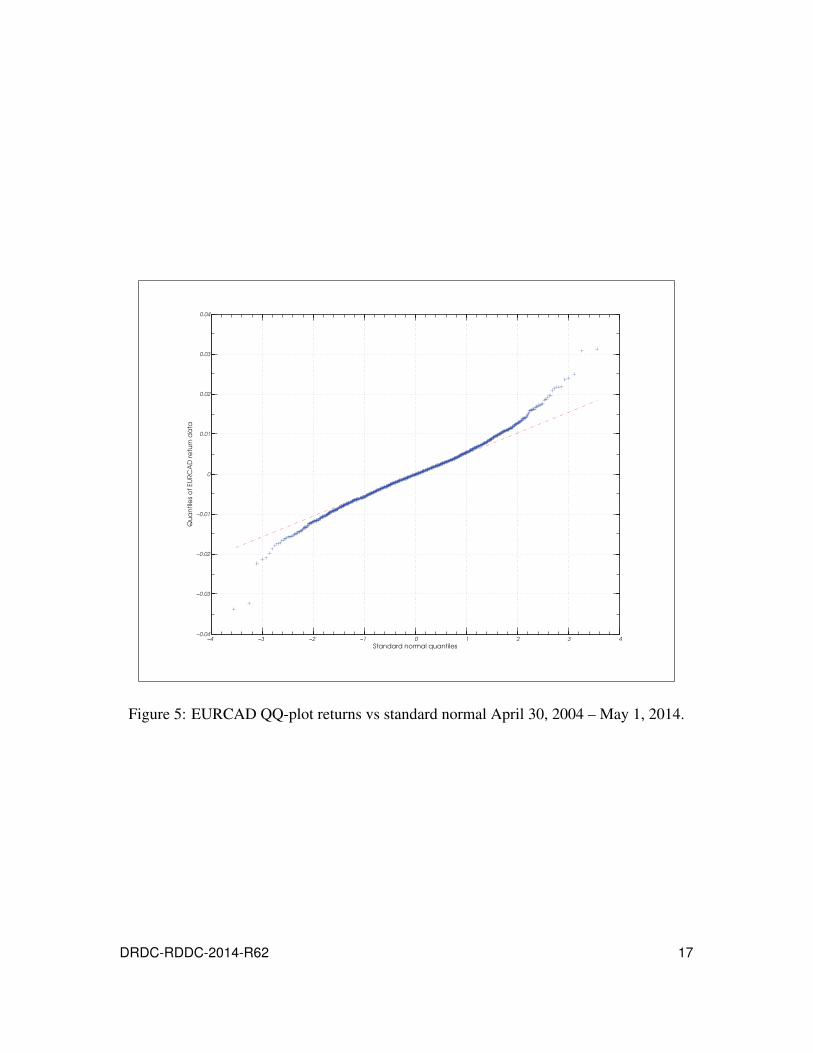
Figure 5: EURCAD QQ-plot returns vs standard normal April 30, 2004 – May

1, 2014. . . . . . . . . . . . . . . . . . . . . . . . . . . . . . . . . . . 17

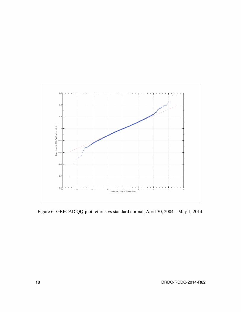
Figure 6: GBPCAD QQ-plot returns vs standard normal, April 30, 2004 – May

1, 2014. . . . . . . . . . . . . . . . . . . . . . . . . . . . . . . . . . . 18

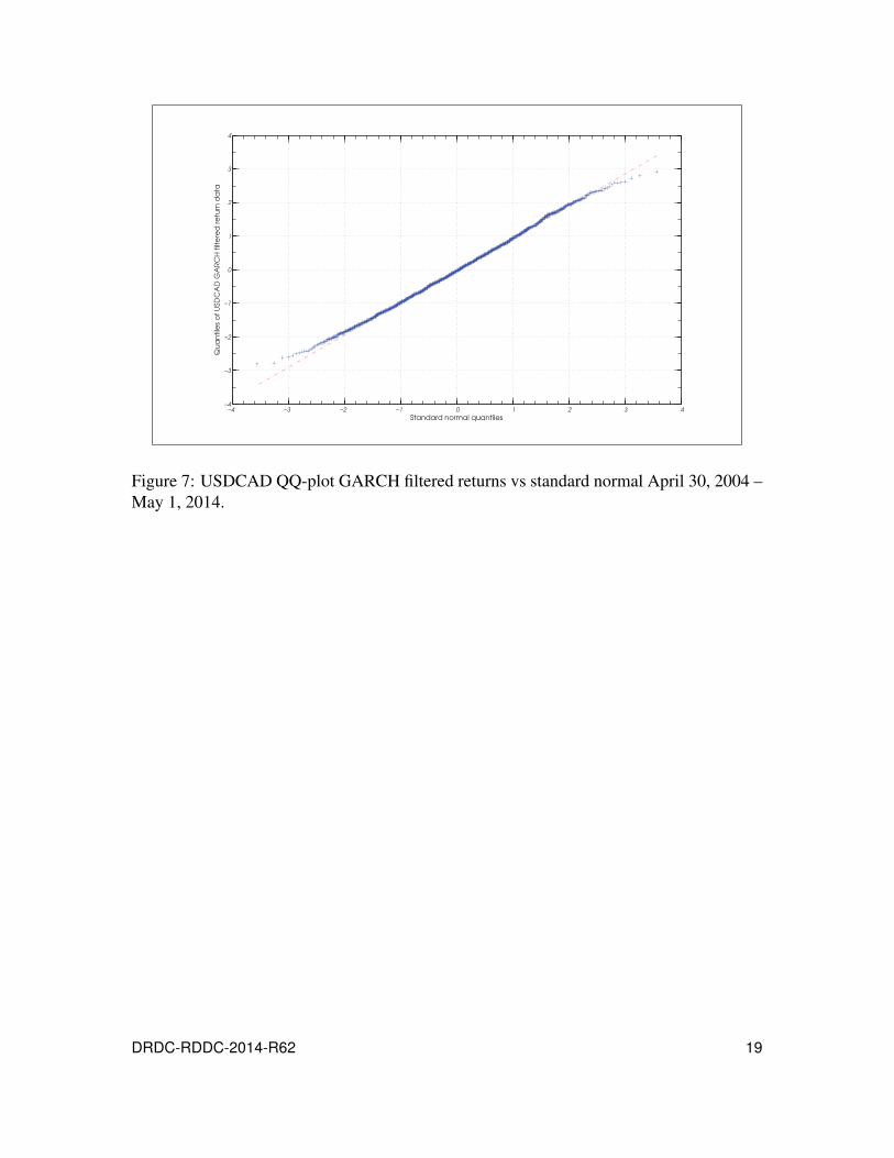
Figure 7: USDCAD QQ-plot GARCH filtered returns vs standard normal April

30, 2004 – May 1, 2014. . . . . . . . . . . . . . . . . . . . . . . . . . 19

Figure 8: EURCAD QQ-plot GARCH filtered returns vs standard normal April

30, 2004 – May 1, 2014. . . . . . . . . . . . . . . . . . . . . . . . . . 20

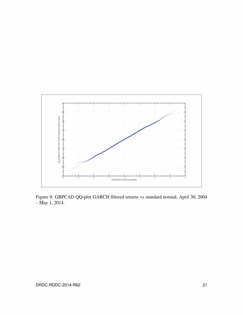
Figure 9: GBPCAD QQ-plot GARCH filtered returns vs standard normal, April

30, 2004 – May 1, 2014. . . . . . . . . . . . . . . . . . . . . . . . . . 21

Figure 10: USDCAD GARCH modelled annualized volatility April 30, 2004 –

May 1, 2014. . . . . . . . . . . . . . . . . . . . . . . . . . . . . . . . 22

Figure 11: EURCAD GARCH modelled annualized volatility April 30, 2004 –

May 1, 2014. . . . . . . . . . . . . . . . . . . . . . . . . . . . . . . . 23

Figure 12: GBPCAD GARCH modelled annualized volatility, April 30, 2004 –

May 1, 2014. . . . . . . . . . . . . . . . . . . . . . . . . . . . . . . . 24

Figure 13: The correlation coefficient for the EURCAD-USDCAD pair April 30,

2004 – May 1, 2014. . . . . . . . . . . . . . . . . . . . . . . . . . . . 25

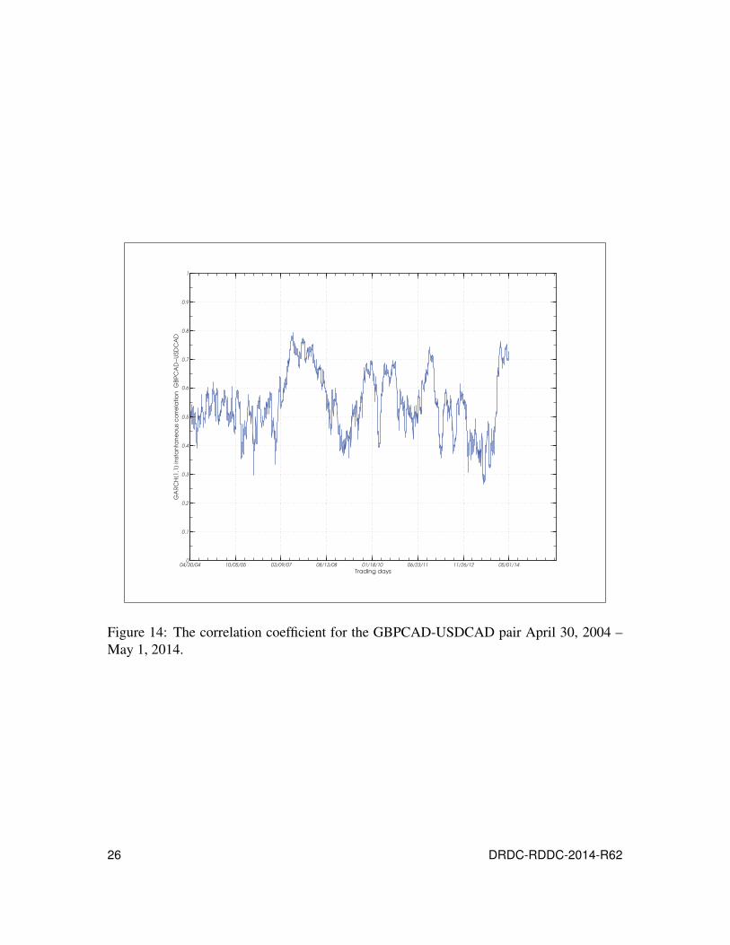
Figure 14: The correlation coefficient for the GBPCAD-USDCAD pair April 30,

2004 – May 1, 2014. . . . . . . . . . . . . . . . . . . . . . . . . . . . 26

Figure 15: EURCAD-USDCAD marginals, April 30, 2004 – May 1, 2014. . . . . . 27

Figure 16: GBPCAD-USDCAD marginals, April 30, 2004 – May 1, 2014. . . . . . 28

vi DRDC-RDDC-2014-R62

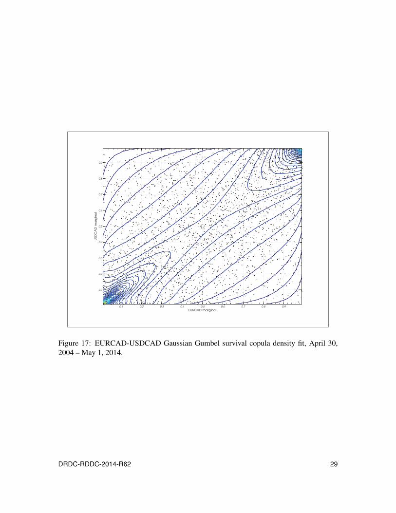
Figure 17: EURCAD-USDCAD Gaussian Gumbel survival copula density fit,

April 30, 2004 – May 1, 2014. . . . . . . . . . . . . . . . . . . . . . . 29

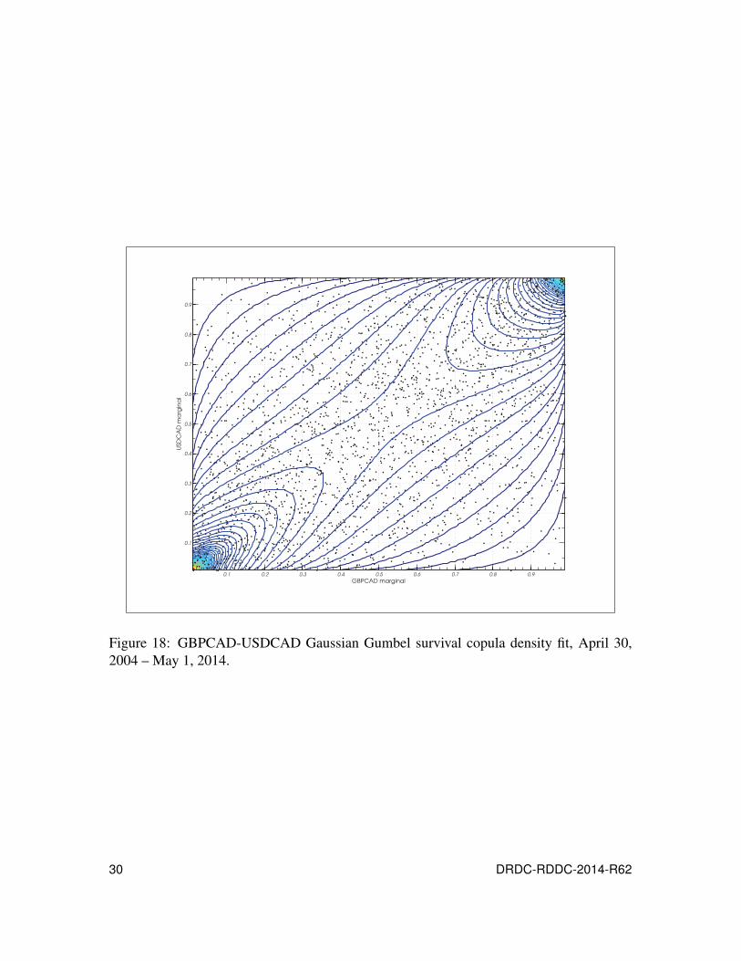
Figure 18: GBPCAD-USDCAD Gaussian Gumbel survival copula density fit,

April 30, 2004 – May 1, 2014. . . . . . . . . . . . . . . . . . . . . . . 30

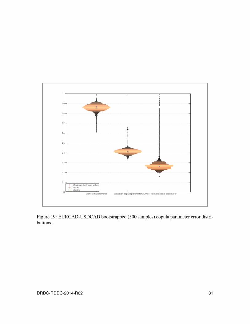
Figure 19: EURCAD-USDCAD bootstrapped (500 samples) copula parameter

error distributions. . . . . . . . . . . . . . . . . . . . . . . . . . . . . . 31

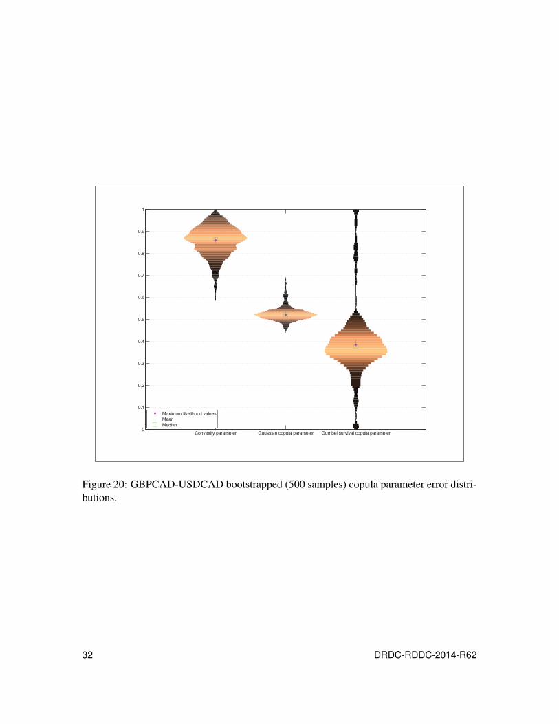
Figure 20: GBPCAD-USDCAD bootstrapped (500 samples) copula parameter

error distributions. . . . . . . . . . . . . . . . . . . . . . . . . . . . . . 32

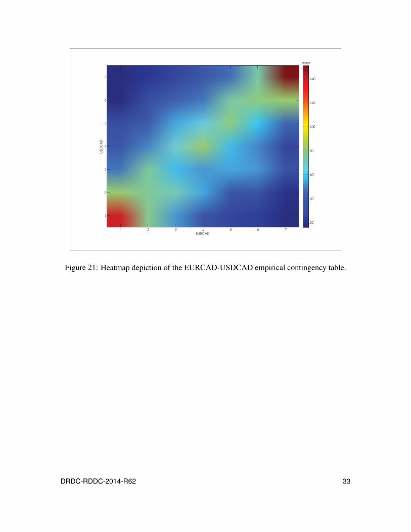
Figure 21: Heatmap depiction of the EURCAD-USDCAD empirical contingency

table. . . . . . . . . . . . . . . . . . . . . . . . . . . . . . . . . . . . . 33

Figure 22: Heatmap depiction of the EURCAD-USDCAD copula predicted

contingency table. . . . . . . . . . . . . . . . . . . . . . . . . . . . . . 34

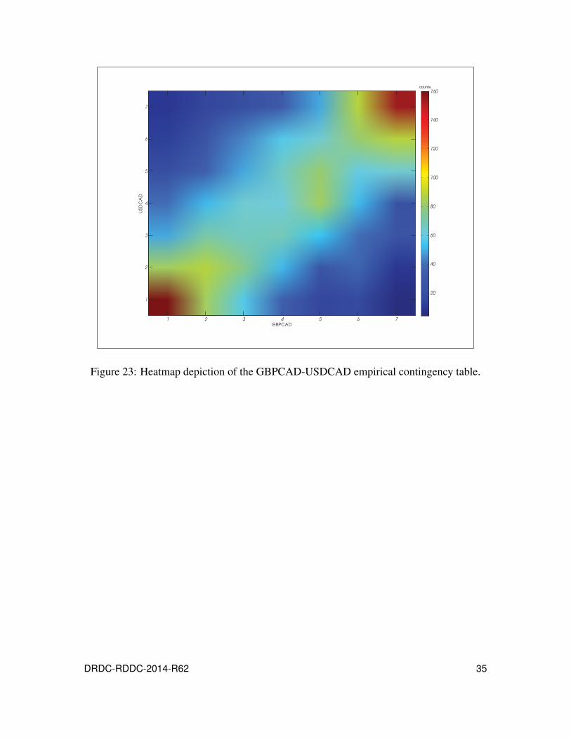
Figure 23: Heatmap depiction of the GBPCAD-USDCAD empirical contingency

table. . . . . . . . . . . . . . . . . . . . . . . . . . . . . . . . . . . . . 35

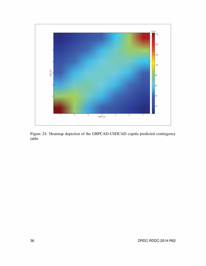
Figure 24: Heatmap depiction of the GBPCAD-USDCAD copula predicted

contingency table. . . . . . . . . . . . . . . . . . . . . . . . . . . . . . 36

Figure 25: GBPCAD-USDCAD simulation: copula scatter plot 100 trading day

horizon from May 1, 2014 (1000 points). . . . . . . . . . . . . . . . . . 38

Figure 26: GBPCAD-USDCAD simulation: multivariate GARCH scatter plot

100 trading day horizon from May 1, 2014 (1000 points). . . . . . . . . 39

DRDC-RDDC-2014-R62 vii

This page intentionally left blank.

viii DRDC-RDDC-2014-R62

1 Introduction1.1 BackgroundThe Department of National Defence (DND) expends approximately 10% of its annual

budget in foreign currencies in support of equipment, acquisitions, and operations. The for-

eign currency transactions within DND’s budget expose the department to financial market

risk in the form of fluctuating exchange rates, placing additional risk mitigation pressures

on internal management. Given the Government of Canada’s planned military acquisitions

in the form of the CF-188 replacement and the renewal of the Royal Canadian Navy –

both of which will contain significant foreign content – foreign exchange risk has quickly

become an important risk element for DND management to understand.

Over the last seven years, the Centre for Operational Research and Analysis (CORA) has

developed in-house financial risk management tools to help DND understand foreign ex-

change market risk within its budgets [1], [2]. CORA’s approach uses two main lines

of inquiry – models based on Generalized Autoregressive Conditional Heteroskedasticity

(GARCH) [1], and models based on the internal consistency of foreign exchange derivative

prices [2]. Both modelling methods yield value-at-risk (VaR) [3]: given a confidence level

p, and a prescribed time horizon T , the VaR yields the foreign exchange loss level that

is exceeded with probability 1− p at time T . Decision makers can use VaR calculations

matched to foreign payment schedules to assess the likelihood of project budget shortfalls.

In conjunction with risk modelling, CORA has helped DND prioritize corporate risk by

using expert opinion with rank correlation. The analysis showed that “increased financial

pressure due to external factors represents one of the highest risk factors among all corpo-

rate activities at DND” [4]. Specifically, ADM(Fin-CS) and ADM(Mat) singled out foreign

exchange risk as a significant liability. Senior decision makers at DND continue to hold

the view that foreign exchange represents a significant risk in DND planning activities.

In this study, we extend our in-house GARCH models to help DND understand the ex-

tent of risk mitigation that occurs naturally through exposure to more than one currency.

DND’s main foreign currency exposure involves the US dollar, the euro, and the British

pound sterling. To gauge the effect of adverse currency fluctuations on DND’s budgets and

planning, we require an understanding of the strength of natural diversification benefits

within VaR analyses. We examine two methods to attack this problem. Our first approach

uses multivariate GARCH models which extract time dependence and persistence in corre-

lations between exchange rate pairs. While this method offers a powerful modelling tool,

the method implicitly contains restrictive assumptions about the nature of the dependency

between the two exchange rates. We address these shortcomings in our second approach by

building dependency models between exchange rate pairs using copulas. Both modelling

techniques offer decision makers a deeper understanding of portfolio VaR in which more

than one currency affects total project costs.

DRDC-RDDC-2014-R62 1

1.2 ScopeADM(FinCS) requires an understanding of foreign exchange risk using VaR calculations

for its budgets. In this paper, we propose a VaR analysis based two methods:

• multivariate GARCH models; and

• copula-GARCH models.

We apply these techniques to EURCAD-USDCAD, and GBPCAD-USDCAD exchange

rate pairings using daily data from April 30, 2004 to May 1, 2014.

2 DRDC-RDDC-2014-R62

2 Generalized autoregressive conditionalheteroskedasticity (GARCH) basics

Foreign exchange markets show no evidence of autocorrelation in the return data, implying

that past observations of foreign exchange prices do not help forecast future returns. This

observation – that past prices offer no predictive power and thus no advantage in trading –

conforms with the efficient market hypothesis (EMH)[5]. However, even though uncondi-

tionally return variances are nearly stationary1, for most assets, and especially for foreign

exchange, they are not conditionally stationary. To understand the return sequence of for-

eign exchange data, we must account for time changing conditional return variances. The

framework for modelling this phenomenon is called generalized autoregressive conditional

heteroskedasticity (GARCH) [7] (see [8] for a complete review).

Under the simplest GARCH model, called GARCH(1,1), the variance process takes the

form,

σ2t+1 = ω +αR2

t +βσ2t , (1)

where α +β < 1 and Rt denotes the asset return. In this paper, we use the arithmetic return,

Rt =St+1 −St

St, (2)

where St is the observed exchange rate at market close.2 In GARCH modelling, we assume

that the return sequence follows,

Rt = σt zt , (3)

where zt follows an iid process.

In addition to modelling univariate time series with GARCH models, we can model the

linear correlation between time series using similar methods. Note that we can re-write

the univariate GARCH(1,1) model by recognizing that the unconditional variance has the

relationship,

σ2 = E(σ2t+1) = ω +αE(R2

t )+βE(σ2t ) (4)

= ω +ασ2 +βσ2, implying,

σ2 =ω

1−α −β,

where we assume that the daily return has a vanishing expectation. Using this approach,

we can eliminate ω from the equations, allowing us to write the bivariate GARCH(1,1)

1For details on long term predictability in asset returns, see [6].2In the literature, log differences are often taken as the return, but we conform to the approach taken in

[9]. Note that for small changes, log and arithmetic returns are nearly identical.


process as,

Qt+1 = E(zt ztrt )(1−α −β )+α(zt ztr

t )+βQt

=

(q11,t+1 q12,t+1

q12,t+1 q22,t+1

)

=

(1 ρρ 1

)(1−α −β )

+α(

z21,t z1,t z2,t

z1,t z2,t z22,t

)+β

(q11,t q12,tq12,t q22,t

), (5)

where

ρt+1 =q12,t+1√q11,t+1q22,t+1

(6)

and zi,t denotes the i-th univariate GARCH filtered return. The unconditional correlation

coefficient is given by,

ρ =1

T

T

∑t=1

z1,t z2,t . (7)

The multivariate GARCH model allows us to track the time dependence and the persistence

of the correlation coefficient. Again, we use maximum likelihood methods for parameter

estimation. The underlying structure of the multivariate GARCH model is a bivariate nor-

mal distribution with a time changing correlation coefficient.


3 A brief introduction to copulas

In statistical modelling, we often desire an understanding of the full joint distribution func-

tion of a collection of random variables. For example, the 2-dimensional case with random

variables, X and Y , have the joint distribution function,

P(X ≤ x,Y ≤ y) = H(x,y), (8)

and in an optimal decision making context, we might require an inference of H(x,y) from

the empirical data. When confronted with the problem of estimating the dependence be-

tween random variables, we often rely on key statistical parameters, such as the covariance

or the correlation coefficient. Unfortunately, dependence runs far deeper than simple co-

variances.

To gain an appreciation of the problem at hand, suppose that we make independent draws

from the standard normal, keeping the result and its square – that is, we construct the

bivariate process (X ,X2). Clearly X2 depends perfectly on X , knowledge of the draw

implies complete knowledge of its square. But notice that the covariance vanishes,

cov(X ,X2) =∫ ∞

−∞x3e

x2

2 dx−(∫ ∞

−∞xe

x2

2 dx)(∫ ∞

−∞x2e

x2

2 dx)= 0. (9)

Thus, even though we know the second of our random variables depends explicitly on the

first, the standard covariance relationship fails to help us understand dependence. While

the correlation coefficient captures linear dependence between random variables, we miss

all the non-linear information.

Copulas address this problem by specifying a parametric distribution from the marginals

of the random variables.3

To begin our introduction to copulas, we require some definitions. We follow [10] and [11]

throughout.

Definition 1 Let S1, . . . ,Sn be non-empty subsets in the extended real number line, R,

[−∞,∞]. Let H be a real function of n variables such that Dom H = S1 ×·· ·× Sn and for

n-tuples a ≤ b (ak ≤ bk for all k) let B = [a, b] = [a1,b1]×·· ·× [an,bn] be an n-box whose

vertices are in Dom H. Then the H-volume of B is given by,

VH(B) = ∑c

sgn(c)H(c), (10)

3Readers familiar with Kendall’s tau and Spearman’s rho for testing statistical dependence will find cou-

plas a powerful tool. Both Kendall’s tau and Spearman’s rho can be re-expressed as integrals over copulas

which generate extra insight into concordance relationships between random variables. For further details

see [10].


where the sum over c is over all vertices of B and sgn(c) denotes,

sgn(c) ={

1 if ck = ak for an even number of k′s,−1 if ck = ak for an odd number of k′s. (11)

�

For example, if B is the 3-box [x1,x2]× [y1,y2]× [z1,z2], then the H-volume of B reads,

VH(B) = H(x2,y2,z2)−H(x2,y2,z1)−H(x2,y1,z2)−H(x1,y2,z2)

+H(x2,y1,z1)+H(x1,y2,z1)+H(x1,y1,z2)−H(x1,y1,z1). (12)

In more compact notation, we write,

VH(B) = ΔbaH(t) = Δbn

an. . .Δb1

a1H(t) (13)

where,

Δbkak

H(t) = H(t1, t2, . . . ,bk, tk+1, . . . , tn)−H(t1, t2, . . . ,ak, tk+1, . . . , tn). (14)

Definition 2 A real function H of n variables is n-increasing if VH(B) ≥ 0 for all n-boxes

whose verticies lie in Dom H. �

We say that the function H is grounded if H(t) = 0 for all t in Dom H such that tk = ak for

at least one k.

Definition 3 An n-dimensional distribution is a function H with domain in Rn such that H

is grounded, n-increasing and H(∞, . . . ,∞) = 1. �

If each Sk has an greatest element, bk, then H has margins, given by

Hk(x) = H(b1, . . . ,bk−1,x,bk+1, . . . ,bn). (15)

We obtain higher dimensional margins by fixing fewer places.

Definition 4 An n-dimensional copula is a function C with domain [0,1]n such that:

• C is grounded and n-increasing;

• C has margins Ck, k = 1,2, . . . ,n, which satisfy Ck(u) = u for all u in [0,1].

�

The above definitions lead us to Sklar’s Theorem:

Theorem 1 (Sklar’s Theorem) Let H be an n-dimensional distribution function with mar-

gins F1, . . . ,Fn. Then there exists and n-copula C such that for all x in Rn,


H(x1, . . . ,xn) =C(F1(x1), . . . ,Fn(xn)). (16)

If F1, . . . ,Fn are all continuous, then C is unique, otherwise C is uniquely determined on

RanF1 ×·· ·×RanFn. Conversely, if C is an n-copula and F1, . . . ,Fn are distribution func-

tions, then the function H defined aboves is an n-dimensional distribution function with

margins F1, . . . ,Fn. For proof, see [10]. �

Corollary 1 Let H be an n-dimensional distribution function with continuous margins

F1, . . . ,Fn and copula C. Then for any u in [0,1]n,

C(u1, . . . ,un) = H(F−11 (u1), . . . ,F−1

n (un)). (17)

Again, see [10] for details. �

From a model building persepective, copulas allow us to build joint distribution functions

from the marginals of individual random variables. In this paper, we will restrict ourselves

to 2-dimensional copulas, namely,

H(x,y) =C(u,v) =C(F−1(x),G−1(y)), (18)

where F(x) and G(x) denote the respective 1-dimensional distribution functions of each

random variable. We concentrate on two copula types:

Gaussian Copula:

CN(u,v;ρ) = ΦN(Φ−1(u),Φ−1(v);ρ)

=1

2π(1−ρ2)1/2

∫ Φ−1(u)

−∞

∫ Φ−1(v)

−∞exp

(−(s2 −2ρst + t2)

2(1−ρ2)

)dsdt, (19)

where Φ(·) is the standard normal distribution function.

Gumbel Copula and the Gumbel Survival Copula:

CG(u,v;α) = exp[−{(− log(u))1/α +(− log(v))1/α

}α](20)

CGS(u,v;α) = u+ v−1+CG(1−u,1− v). (21)

We can easily show that the convex sum of copulas is also a copula, and thus we consider

two model class for our foreign exchange analysis

C1(u,v;θ ,ρ,α) = (1−θ)CN(u,v;ρ)+θCG(u,v;α)

C2(u,v;θ ,ρ,α) = (1−θ)CN(u,v;ρ)+θCGS(u,v;α) (22)

where the convexity parameter satisfies θ ∈ [0,1]. Using maximum likelihood estimations,

we can determine which model best describes the foreign exchange data.


Our coupla selection offers a wide range of dependency fitting potential with parsimony

[12]. The foreign exchange data exhibits features contained in both copula classes. The

Gaussian copula belongs to a symmetric multivariate elliptical family – a feature that for-

eign exchange data exhibits at a gross level – and the Gumbel (survival) captures strong

right (left) tail dependence, allowing us to model asymmetrical fat tails. In principle, we

could create a five dimensional model by using a convex sum of the Gaussian, Gumbel, and

Gumbel survival copula, but we find that the reduced parsimony does not give qualitative

better results.

Once we have a copula fit to the data, we require a method for sampling to generate Monte

Carlo simulations. Observe that,

P(V ≤ v|U = u) = limΔu→0

C(u+Δu,v)−C(u,v)Δu

=Cu(u,v). (23)

Thus we can calculate the conditional probability by taking the derivative of the copula with

respect to one of its arguments. To sample from a copula, we generate two realizations from

the uniform distribution, u, and t, and then solve

Cu(u,v) = t, (24)

for v. The resulting pair, (u,v), represents the value of each marginal sampled from the cop-

ula. Inverting the marginals u = F(x), and v = G(y), we obtain the Monte Carlo realization

of our random variables.


4 Foreign exchange data and analysis

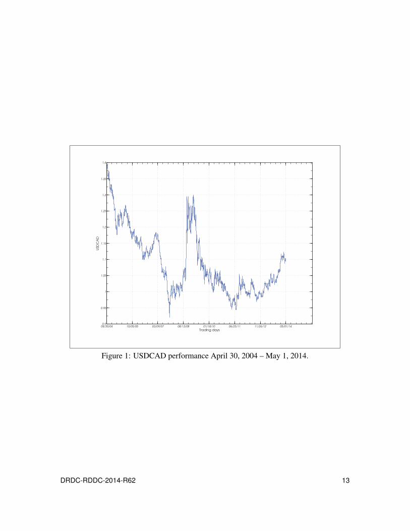
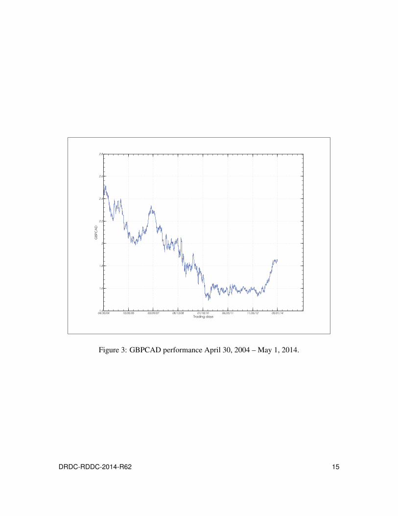
We use ten years of foreign exchange data [13], 30 April 2004 to 1 May 2014, for USD-

CAD, EURCAD, and GBPCAD, giving a total of 2609 observations in each time series.

Figures 1, 2, 3 show the historical observations. DND’s largest foreign exchange expo-

sure is the USDCAD, followed by EURCAD, and GBPCAD [1] and we therefore focus

on the pairwise dependency relationship between the USDCAD and DND’s more minor

exposures. From a risk analysis perspective, since the USDCAD dominates DND’s foreign

exchange obligations, any diversification benefit comes primarily from the USDCAD’s re-

lationship to the other two currencies.

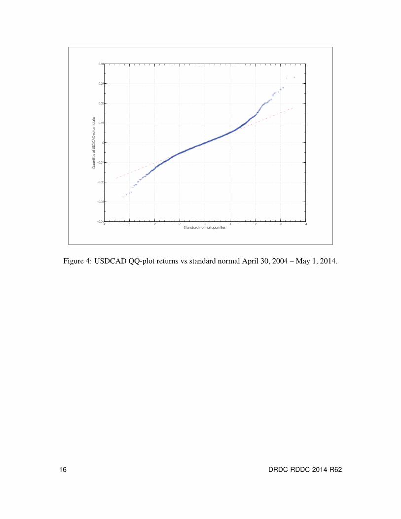
In the QQ-plots of Figures 4, 5, and 6 we immediately see that the financial return data is

not iidN(0,1). We fit GARCH(1,1) models to our data using quasi-maximum likelihood

methods [8]. Using the Kolmogorov-Smirnov test on the filtered returns, we find that we

cannot reject the null hypothesis that the innovations for each times belong to iidN(0,1).The QQ-plots of Figures 7, 8, and 9 show the quality of the GARCH filtered returns relative

to the standard normal.

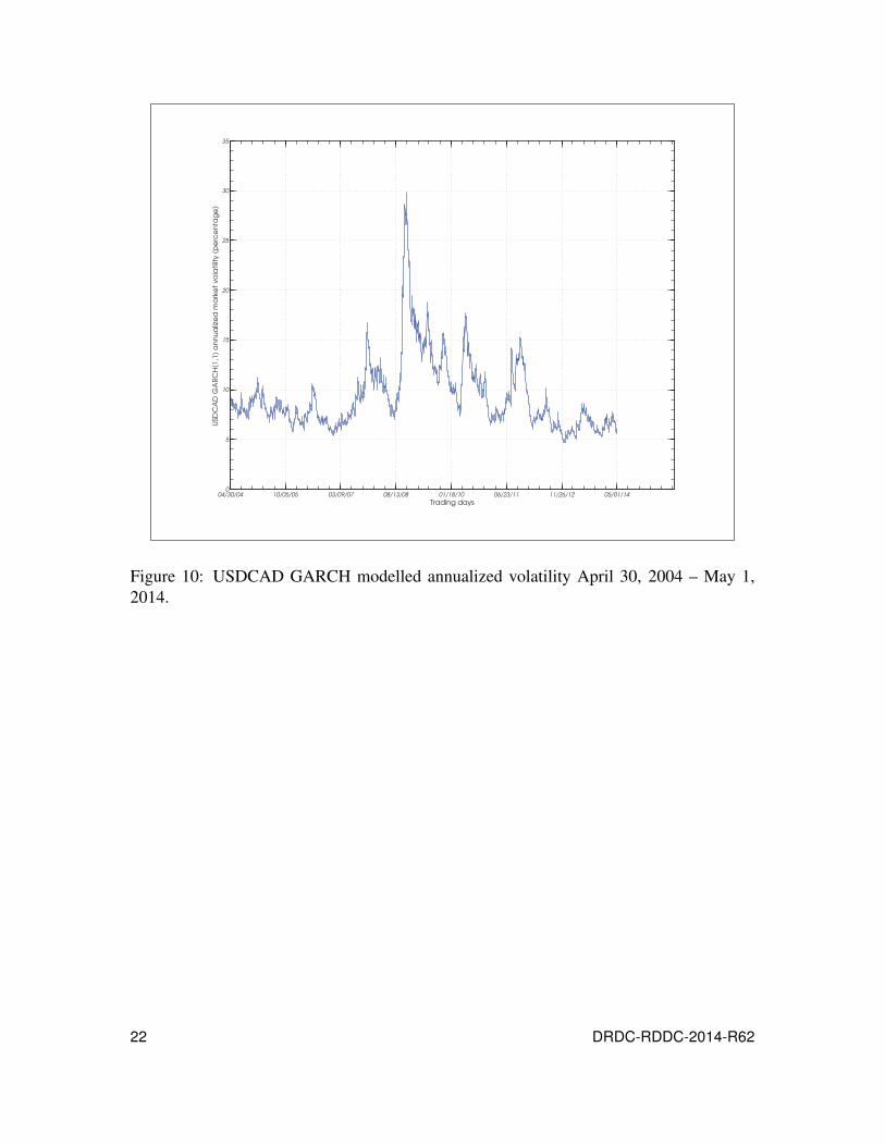
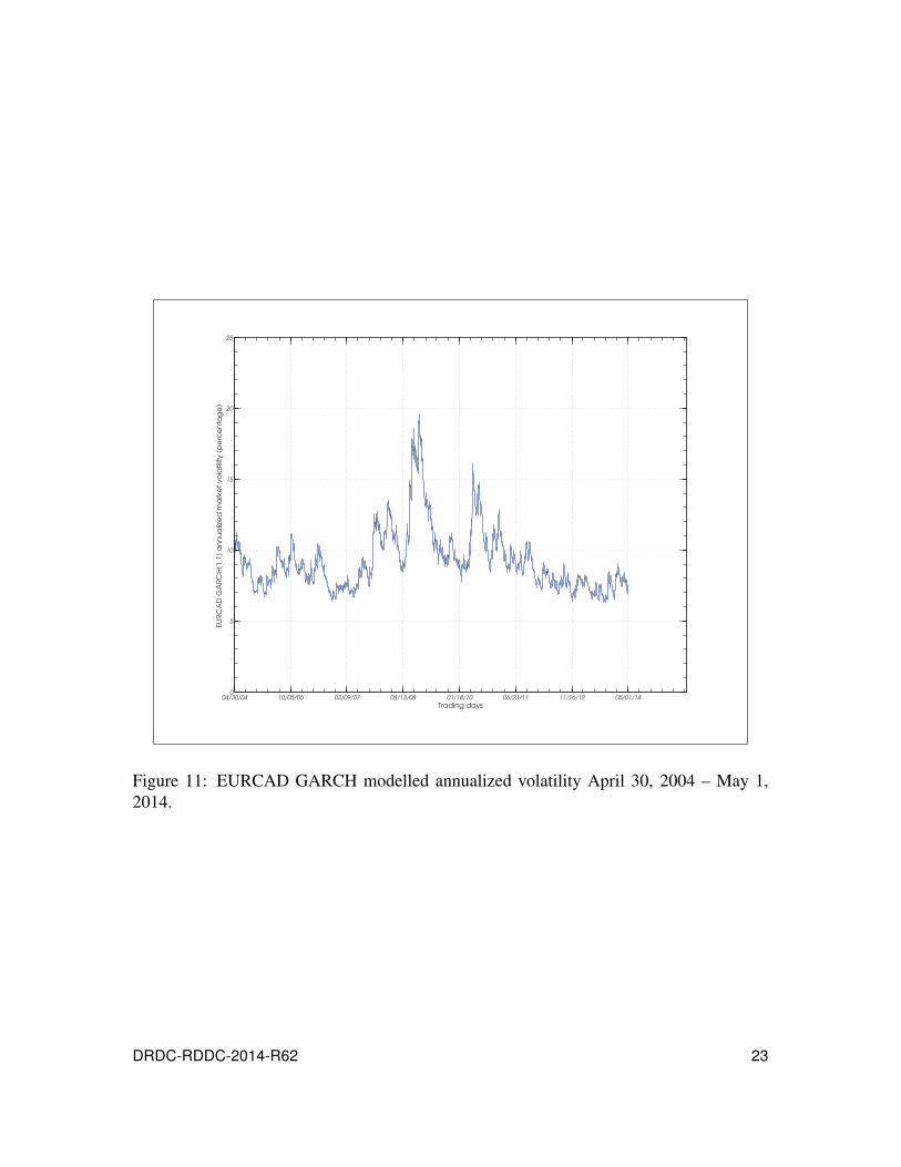
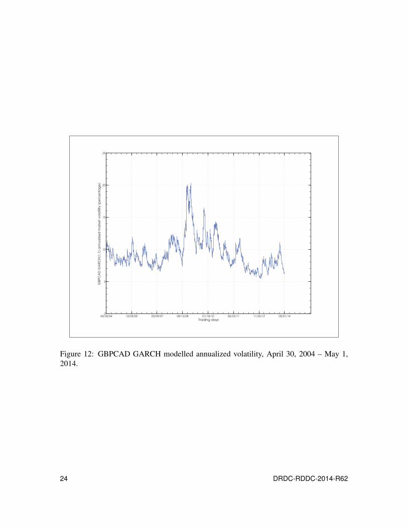
In Figures 10, 11, and 12 we see the time changing stochastic volatility for each time

series expressed as an annualized percentage. Notice the sharp rise in volatility beginning

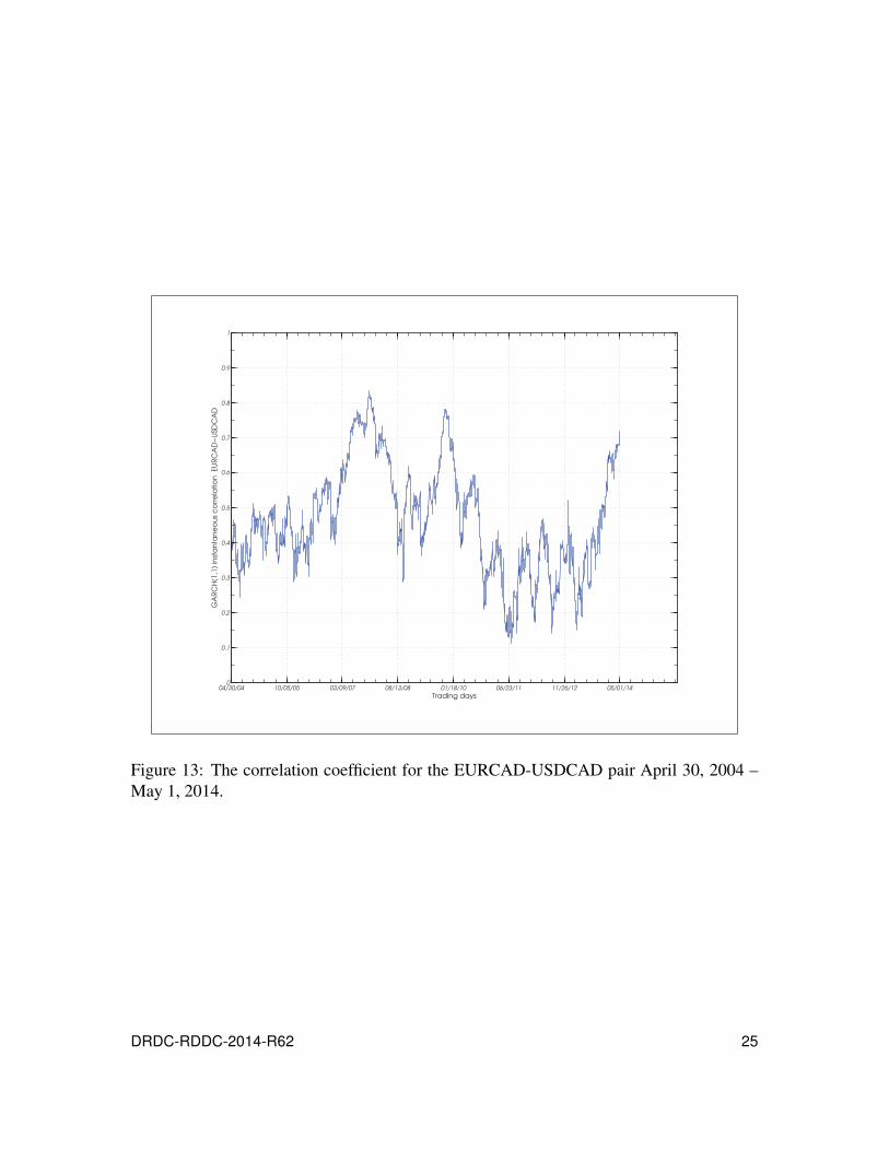
in late September 2008, demarking the onset of the financial crisis. Using the GARCH

filtered return data, we compute the dynamics of the linear correlation coefficient between

the currency pairs EURCAD-USDCAD and GBPCAD-USDCAD; we display the results

in Figures 13, and 14.

While the multivariate GARCH model captures time dependence and persistence, it does

not allow asymmetrical heavy tailed relationships between pairs of time series. To reveal

these features in the data, we use convex sums of Gaussian, and Gumbel (survival) copulas.

We take each GARCH filtered time series pair and convert the data to their marginals. We

do not parametrically model the marginals, instead relying on the empirical distribution

functions themselves (recall that the Kolmogorov-Smirnov test does not reject N(0,1) as

the distribution function for each GARCH filtered return time series). In Figures 15, and

16 we see the scatter plots in the marginal space which immediately show a Southwest to

Northeast direction – the time series pairs exhibit dependence, which we already discovered

using the multivariate GARCH technique. Fitting the convex copula sum, we find that the

Gaussian and Gumbel survival copula summed together provide the best fit to the data

for both time series pairs. We show in Figures 17 and 18 the scatter plot data of Figures

15, and 16 with the iso-contours of the best fit copula density function. The effect of the

asymmetric tail, captured by the Gumbel survival copula component, is readily apparent.

To examine the robustness of our result, we perform a 500 sample bootstrap of the data to

generate error estimates on each parameter of the copula model. We show the bootstrap

results in Figure 19 and Figure 20.


We test each copula model for time dependence in each of its parameters in turn, holding

the others fixed, by partitioning the data according to a 4×4 grid of the unit square. Each

of the copula parameters Θ = (θ ,ρ,α), belong to the grid through the sum,

Θi,t =16

∑j

d j[(z1,t−1,z2,t−1) ∈ A j] (25)

where A j corresponds to the j-th element of the partitioned unit square and d j is the 16-

tuple, (d1,d2, . . . ,d16), extension of the copula parameter considered. For example, A1 =[0, p1)× [0,q1); A2 = [p1, p2)× [0,q1]; etc. The choice of the partition is arbitrary and we

follow [14], by setting (p,q) ∈ (0.15,0.50,0.85) to ensure that we focus on large values

within the partition elements. Thus the likelihood sum becomes,

Θi = argminT

∑t=1

ln(c(u1,u2);Γ(z1,t−1,z2,t−1;Θi)) , (26)

where c(u1,u2) is the copula density as a function of the empirical marginals and,

Γ(z1,t−1,z2,t−1;Θi), (27)

corresponds to the selection procedure of eq.(25). While this process can elicit time depen-

dence, it cannot reveal persistence as in the multivariate GARCH estimation (the partition

method looks back only one time step). The maximum likelihood method allows us to esti-

mate each d j (16-tuple) along with its standard error, which allows us to test for statistical

significance in differences by using the χ2(15) test [14]. We do not find evidence for time

dependence in any of the copula parameters for each of the time series pairs.

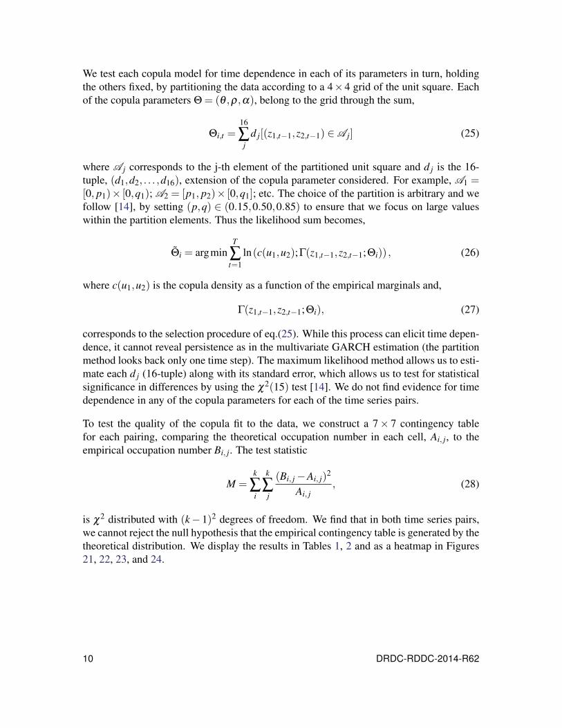
To test the quality of the copula fit to the data, we construct a 7× 7 contingency table

for each pairing, comparing the theoretical occupation number in each cell, Ai, j, to the

empirical occupation number Bi, j. The test statistic

M =k

∑i

k

∑j

(Bi, j −Ai, j)2

Ai, j, (28)

is χ2 distributed with (k− 1)2 degrees of freedom. We find that in both time series pairs,

we cannot reject the null hypothesis that the empirical contingency table is generated by the

theoretical distribution. We display the results in Tables 1, 2 and as a heatmap in Figures

21, 22, 23, and 24.


Table 1: Seven quantile contingency table test for the copula fit to EURCAD - USDCAD.

Quantile counts

Exchange rate pairings 1st 2nd 3rd 4th 5th 6th 7th χ2(36)

EURCAD-USDCAD (empirical)

Quantile counts

7th 16 21 26 38 46 74 151

6th 18 29 42 48 74 80 82

5th 30 40 55 63 81 60 44

4th 38 51 68 82 57 51 25

3rd 48 77 57 52 54 52 33

2nd 83 77 72 54 35 32 20

1st 139 78 53 35 26 24 17

EURCAD-USDCAD (predicted)

Quantile counts

7th 10 20 29 40 54 79 139

6th 20 33 41 52 66 81 79

5th 29 41 50 62 70 66 54

4th 39 50 62 69 62 52 40

3rd 52 65 73 62 50 41 29

2nd 76 88 65 50 41 33 20

1st 146 76 52 39 29 20 10 43.4 (c.v. 51.0)


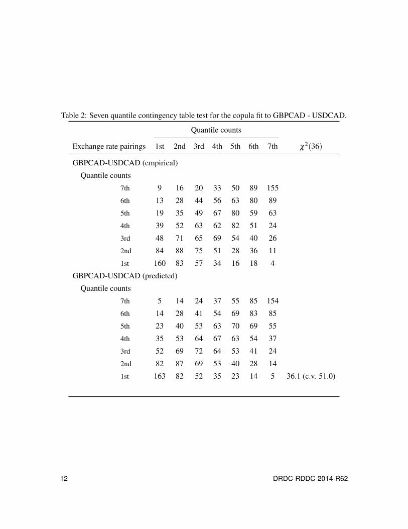
Table 2: Seven quantile contingency table test for the copula fit to GBPCAD - USDCAD.

Quantile counts

Exchange rate pairings 1st 2nd 3rd 4th 5th 6th 7th χ2(36)

GBPCAD-USDCAD (empirical)

Quantile counts

7th 9 16 20 33 50 89 155

6th 13 28 44 56 63 80 89

5th 19 35 49 67 80 59 63

4th 39 52 63 62 82 51 24

3rd 48 71 65 69 54 40 26

2nd 84 88 75 51 28 36 11

1st 160 83 57 34 16 18 4

GBPCAD-USDCAD (predicted)

Quantile counts

7th 5 14 24 37 55 85 154

6th 14 28 41 54 69 83 85

5th 23 40 53 63 70 69 55

4th 35 53 64 67 63 54 37

3rd 52 69 72 64 53 41 24

2nd 82 87 69 53 40 28 14

1st 163 82 52 35 23 14 5 36.1 (c.v. 51.0)


Trading days

USD

CA

D

04/30/04 10/05/05 03/09/07 08/13/08 01/18/10 06/23/11 11/26/12 05/01/140.9

0.95

1

1.05

1.1

1.15

1.2

1.25

1.3

1.35

1.4

Figure 1: USDCAD performance April 30, 2004 – May 1, 2014.


Trading days

EUR

CA

D

04/30/04 10/05/05 03/09/07 08/13/08 01/18/10 06/23/11 11/26/12 05/01/14

1.3

1.4

1.5

1.6

1.7

1.8

1.9

Figure 2: EURCAD performance April 30, 2004 – May 1, 2014.


Trading days

GBP

CA

D

04/30/04 10/05/05 03/09/07 08/13/08 01/18/10 06/23/11 11/26/12 05/01/141.4

1.6

1.8

2

2.2

2.4

2.6

2.8

Figure 3: GBPCAD performance April 30, 2004 – May 1, 2014.


Standard normal quantiles

Qu

an

tile

s o

f U

SDC

AD

retu

rn d

ata

−4 −3 −2 −1 0 1 2 3 4−0.04

−0.03

−0.02

−0.01

0

0.01

0.02

0.03

0.04

Figure 4: USDCAD QQ-plot returns vs standard normal April 30, 2004 – May 1, 2014.



Qu

an

tile

s o

f EU

RC

AD

retu

rn d

ata

−4 −3 −2 −1 0 1 2 3 4−0.04

−0.03

−0.02

−0.01

0

0.01

0.02

0.03

0.04

Figure 5: EURCAD QQ-plot returns vs standard normal April 30, 2004 – May 1, 2014.



Qu

an

tile

s o

f G

BPC

AD

retu

rn d

ata

−4 −3 −2 −1 0 1 2 3 4−0.05

−0.04

−0.03

−0.02

−0.01

0

0.01

0.02

0.03

Figure 6: GBPCAD QQ-plot returns vs standard normal, April 30, 2004 – May 1, 2014.



Qu

an

tile

s o

f U

SDC

AD

GA

RC

H f

ilte

red

retu

rn d

ata

−4 −3 −2 −1 0 1 2 3 4−4

−3

−2

−1

0

1

2

3

4

Figure 7: USDCAD QQ-plot GARCH filtered returns vs standard normal April 30, 2004 –

May 1, 2014.



Qu

an

tile

s o

f EU

RC

AD

GA

RC

H f

ilte

red

retu

rn d

ata

−4 −3 −2 −1 0 1 2 3 4−4

−3

−2

−1

0

1

2

3

4

Figure 8: EURCAD QQ-plot GARCH filtered returns vs standard normal April 30, 2004 –

May 1, 2014.



Qu

an

tile

s o

f G

BPC

AD

GA

RC

H f

ilte

red

retu

rn d

ata

−4 −3 −2 −1 0 1 2 3 4−4

−3

−2

−1

0

1

2

3

4

Figure 9: GBPCAD QQ-plot GARCH filtered returns vs standard normal, April 30, 2004

– May 1, 2014.


Trading days

USD

CA

D G

AR

CH

(1,1

) a

nn

ua

lize

d m

ark

et

vola

tility

(p

erc

en

tag

e)

04/30/04 10/05/05 03/09/07 08/13/08 01/18/10 06/23/11 11/26/12 05/01/140

5

10

15

20

25

30

35

Figure 10: USDCAD GARCH modelled annualized volatility April 30, 2004 – May 1,

2014.


Trading days

EUR

CA

D G

AR

CH

(1,1

) a

nn

ua

lize

d m

ark

et

vola

tility

(p

erc

en

tag

e)

04/30/04 10/05/05 03/09/07 08/13/08 01/18/10 06/23/11 11/26/12 05/01/140

5

10

15

20

25

Figure 11: EURCAD GARCH modelled annualized volatility April 30, 2004 – May 1,

2014.


Trading days

GBP

CA

D G

AR

CH

(1,1

) a

nn

ua

lize

d m

ark

et

vola

tility

(p

erc

en

tag

e)

04/30/04 10/05/05 03/09/07 08/13/08 01/18/10 06/23/11 11/26/12 05/01/140

5

10

15

20

25

Figure 12: GBPCAD GARCH modelled annualized volatility, April 30, 2004 – May 1,

2014.


Trading days

GA

RC

H(1

,1)

inst

an

tan

eo

us

co

rre

latio

n E

UR

CA

D−

USD

CA

D

04/30/04 10/05/05 03/09/07 08/13/08 01/18/10 06/23/11 11/26/12 05/01/140

0.1

0.2

0.3

0.4

0.5

0.6

0.7

0.8

0.9

1

Figure 13: The correlation coefficient for the EURCAD-USDCAD pair April 30, 2004 –

May 1, 2014.


Trading days

GA

RC

H(1

,1)

inst

an

tan

eo

us

co

rre

latio

n G

BPC

AD

−U

SDC

AD

04/30/04 10/05/05 03/09/07 08/13/08 01/18/10 06/23/11 11/26/12 05/01/140

0.1

0.2

0.3

0.4

0.5

0.6

0.7

0.8

0.9

1

Figure 14: The correlation coefficient for the GBPCAD-USDCAD pair April 30, 2004 –

May 1, 2014.


EURCAD marginal

USD

CA

D m

arg

ina

l

0 0.1 0.2 0.3 0.4 0.5 0.6 0.7 0.8 0.9 10

0.1

0.2

0.3

0.4

0.5

0.6

0.7

0.8

0.9

1

Figure 15: EURCAD-USDCAD marginals, April 30, 2004 – May 1, 2014.


GBPCAD marginal

USD

CA

D m

arg

ina

l

0 0.1 0.2 0.3 0.4 0.5 0.6 0.7 0.8 0.9 10

0.1

0.2

0.3

0.4

0.5

0.6

0.7

0.8

0.9

1

Figure 16: GBPCAD-USDCAD marginals, April 30, 2004 – May 1, 2014.


EURCAD marginal

USD

CA

D m

arg

ina

l

0.1 0.2 0.3 0.4 0.5 0.6 0.7 0.8 0.9

0.1

0.2

0.3

0.4

0.5

0.6

0.7

0.8

0.9

Figure 17: EURCAD-USDCAD Gaussian Gumbel survival copula density fit, April 30,

2004 – May 1, 2014.


GBPCAD marginal

USD

CA

D m

arg

ina

l

0.1 0.2 0.3 0.4 0.5 0.6 0.7 0.8 0.9

0.1

0.2

0.3

0.4

0.5

0.6

0.7

0.8

0.9

Figure 18: GBPCAD-USDCAD Gaussian Gumbel survival copula density fit, April 30,

2004 – May 1, 2014.


Convexity parameter Gaussian copula parameterGumbel survival copula parameter0

0.1

0.2

0.3

0.4

0.5

0.6

0.7

0.8

0.9

1

Maximum likelihood valuesMeanMedian

Figure 19: EURCAD-USDCAD bootstrapped (500 samples) copula parameter error distri-

butions.


Convexity parameter Gaussian copula parameter Gumbel survival copula parameter0

0.1

0.2

0.3

0.4

0.5

0.6

0.7

0.8

0.9

1

Maximum likelihood valuesMeanMedian

Figure 20: GBPCAD-USDCAD bootstrapped (500 samples) copula parameter error distri-

butions.


EURCAD

USD

CA

D

1 2 3 4 5 6 7

7

6

5

4

3

2

1

counts

20

40

60

80

100

120

140

Figure 21: Heatmap depiction of the EURCAD-USDCAD empirical contingency table.


EURCAD

USD

CA

D

1 2 3 4 5 6 7

7

6

5

4

3

2

1

counts

20

40

60

80

100

120

140

Figure 22: Heatmap depiction of the EURCAD-USDCAD copula predicted contingency

table.


GBPCAD

USD

CA

D

1 2 3 4 5 6 7

7

6

5

4

3

2

1

counts

20

40

60

80

100

120

140

160

Figure 23: Heatmap depiction of the GBPCAD-USDCAD empirical contingency table.


GBPCAD

USD

CA

D

1 2 3 4 5 6 7

7

6

5

4

3

2

1

counts

20

40

60

80

100

120

140

160

Figure 24: Heatmap depiction of the GBPCAD-USDCAD copula predicted contingency

table.


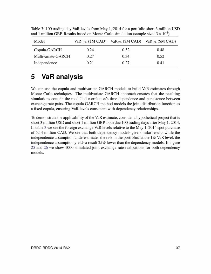
Table 3: 100 trading day VaR levels from May 1, 2014 for a portfolio short 3 million USD

and 1 million GBP. Results based on Monte Carlo simulation (sample size: 3×104).

Model VaR10% ($M CAD) VaR5% ($M CAD) VaR1% ($M CAD)

Copula-GARCH 0.24 0.32 0.48

Multivariate-GARCH 0.27 0.34 0.52

Independence 0.21 0.27 0.41

5 VaR analysis

We can use the copula and multivariate GARCH models to build VaR estimates through

Monte Carlo techniques. The multivariate GARCH approach ensures that the resulting

simulations contain the modelled correlation’s time dependence and persistence between

exchange rate pairs. The copula GARCH method models the joint distribution function as

a fixed copula, ensuring VaR levels consistent with dependency relationships.

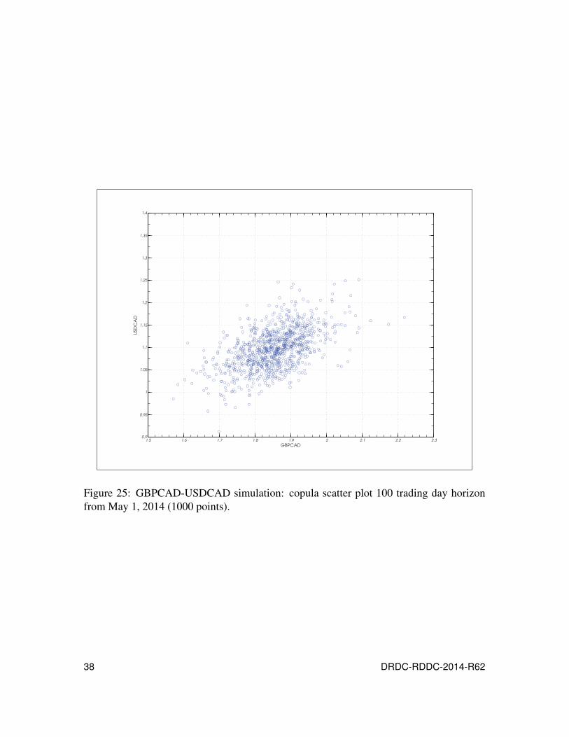
To demonstrate the applicability of the VaR estimate, consider a hypothetical project that is

short 3 million USD and short 1 million GBP, both due 100 trading days after May 1, 2014.

In table 3 we see the foreign exchange VaR levels relative to the May 1, 2014 spot purchase

of 5.14 million CAD. We see that both dependency models give similar results while the

independence assumption underestimates the risk in the portfolio: at the 1% VaR level, the

independence assumption yields a result 25% lower than the dependency models. In figure

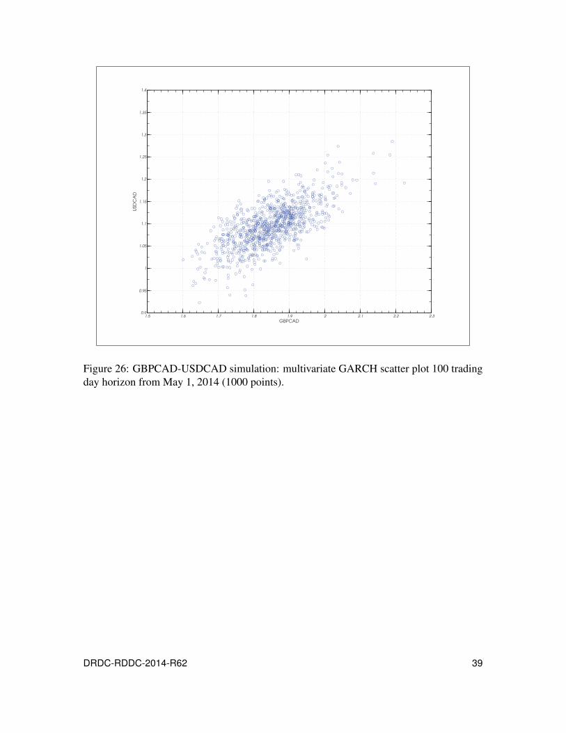
25 and 26 we show 1000 simulated joint exchange rate realizations for both dependency

models.


GBPCAD

USD

CA

D

1.5 1.6 1.7 1.8 1.9 2 2.1 2.2 2.30.9

0.95

1

1.05

1.1

1.15

1.2

1.25

1.3

1.35

1.4

Figure 25: GBPCAD-USDCAD simulation: copula scatter plot 100 trading day horizon

from May 1, 2014 (1000 points).


GBPCAD

USD

CA

D

1.5 1.6 1.7 1.8 1.9 2 2.1 2.2 2.30.9

0.95

1

1.05

1.1

1.15

1.2

1.25

1.3

1.35

1.4

Figure 26: GBPCAD-USDCAD simulation: multivariate GARCH scatter plot 100 trading

day horizon from May 1, 2014 (1000 points).


6 Discussion

We present two methods – the multivariate GARCH, and the copula-GARCH – for esti-

mating the foreign exchange return process. Using both methods, we can compute the VaR

for a portfolio of foreign exchange obligations, properly including the dependence between

currency pairs. We can construct Monte Carlo samples from each model and reverse the

GARCH process to give simulated returns. Both models offer advantages – the multivari-

ate GARCH model captures the persistence of shocks to the correlation coefficient, while

the copula-GARCH model captures asymmetric tail dependence. Using both models will

help DND managers understand multiple foreign currency exposures risk within project

budgets.

We find that the pairings EURCAD-USDCAD and GBPCAD-USDCAD exhibit strong

dependence in both modelling approaches. When the Canadian dollar does well or poor

against one of the currencies, the Canadian dollar tends to follow the same performance

against the other currency. Thus, DND’s multiple currency exposures provides some, but

limited, diversification benefit – especially during tail events.

Senior decision makers can use these models to gauge the foreign exchange risk within

project budgets. We see that the exposure to multiple currencies does not eliminate foreign

exchange risk and we cannot simply convolve distributions from univariate time series for

each currency to estimate portfolio VaR. The dependency between the exchange rates plays

an important role in determining the overall VaR level of the portfolio.

While VaR offers a risk monitoring mechanism for DND, it does not in and of itself offer

risk mitigation. DND must decide on the risks it is comfortable holding. As a cautionary

note, before embarking on any risk mitigation strategy in foreign exchange – contingency

reserve or derivative based – DND must understand the source of possible gains. In fi-

nancial firm evaluation, creating or buying insurance against unfavourable outcomes does

not affect the value of a firm. Insurance repackages the firm’s cash flows, and cash flow

repackaging cannot increase firm value.4 If insurance does provide value, it must come

from advantages that the insurance separately creates. For example, if management can

re-focus its efforts in areas where it has a comparative advantage by entering an insurance

contract, then the repackaging can have a positive effect. In DND’s case, financial risk

mitigation of any kind must be tied to the real source of potential gains – superior project

management.

CORA has afforded DND three powerful methods for modelling and understanding foreign

exchange risk across department budgets: mulitvariate GARCH models, copula-GARCH

models, and models based on the prices of vanilla foreign exchange options (in particular,

the risk neutral probability distribution from the Heston model). Each modelling method

4This is a statement of the famous Modigliani-Miller Theorem – a no arbitrage argument for firm pricing.

See [15] for details.


offers insight into the exchange rate market risk that DND assumes in foreign transactions.

They capture realistic features of market data including heavy tails, asymmetric density

functions, and leptokurtosis. The inclusion of regular VaR updates in risk reporting over

time horizons sensitive to major project deliveries will help senior DND decision makers

better understand their foreign currency liabilities in military operations.


References

[1] Desmier, P. (2007), Estimating Foreign Exchange Exposure in the Department of

National Defence, (DRDC-RDDC-2006-TR023) Defence Research and

Development Canada – CORA.

[2] Maybury, D. (2013), Modelling the US Dollar Trading Range: Bounds from the Risk

Neutral Measure, (DRDC-RDDC-2013-TM086) Defence Research and

Development Canada – Atlantic.

[3] Duffie, D. and Pan, J. (1997), An Overview of Value at Risk, The Journal ofDerivatives, 4(3), 7–49.

[4] Yazbeck, T. (2010), Analytical Support to the Prioritization of Corporate Risks in the

Department of National Defence, (DRDC-RDDC-2010-TM158) Defence Research

and Development Canada – CORA.

[5] Fama, E. (1970), Efficient Capital Markets: A Review of Theory and Empirical

Work, Journal of Finance, 25(2), 383–417.

[6] Cochrane, J. (2005), Asset Pricing, Princeton University Press.

[7] Bollerslev, T. (1986), Generalized Autoregressive Conditional Heteroskedasticity,

Journal of Econometrics, 31(3), 307–27.

[8] Hamilton, J. (1994), Time Series Analysis, Princeton University Press.

[9] Hull, J. (2007), Options, Futures, and Other Derivatives, 6th Ed., Prentice Hall.

[10] Nelsen, R. (2006), An Introduction to Copulas, 2nd Ed., Springer.

[11] Embrechts, P., Lindskog, F., and McNeil, A., Modelling Dependence with Copulas

and Applications to Risk Management.

[12] Hu, L. (2006), Dependence patterns across financial markets: a mixed copula

approach, Applied Financial Economics, 16(10), 717–729.

[13] Bloomberg, L. P., Foreign exchange data EURCAD, GBPCAD, USDCAD 04/30/04

to 05/01/14. Retrieved May 1, 2014.

[14] Jondeau, E. and Rockinger, M. (2006), The Copula-GARCH model of conditional

dependencies: An international stock market application, Journal of InternationalMoney and Finance, 25, 827–853.

[15] Copeland, T., Weston, J., and Shastri, K. (2005), Financial Theory and Corporate

Policy, 4th Ed., Addison Wesley.


DOCUMENT CONTROL DATA(Security markings for the title, abstract and indexing annotation must be entered when the document is Classified or Designated.)

1. ORIGINATOR (The name and address of the organization preparing thedocument. Organizations for whom the document was prepared, e.g. Centresponsoring a contractor’s report, or tasking agency, are entered in section 8.)

DRDC – Centre for Operational Research andAnalysisDept. of National Defence, MGen G. R. Pearkes Bldg.,101 Colonel By Drive, 6CBS, Ottawa ON K1A 0K2,Canada

2a. SECURITY MARKING (Overall securitymarking of the document, includingsupplemental markings if applicable.)

UNCLASSIFIED2b. CONTROLLED GOODS

(NON-CONTROLLEDGOODS)DMC AREVIEW: GCEC APRIL 2011

3. TITLE (The complete document title as indicated on the title page. Its classification should be indicated by the appropriateabbreviation (S, C or U) in parentheses after the title.)

Foreign exchange value-at-risk with multiple currency exposure

4. AUTHORS (Last name, followed by initials – ranks, titles, etc. not to be used.)

Maybury, D. W.

5. DATE OF PUBLICATION (Month and year of publication ofdocument.)

November 2014

6a. NO. OF PAGES (Totalcontaining information.Include Annexes,Appendices, etc.)

54

6b. NO. OF REFS (Totalcited in document.)

157. DESCRIPTIVE NOTES (The category of the document, e.g. technical report, technical note or memorandum. If appropriate, enter

the type of report, e.g. interim, progress, summary, annual or final. Give the inclusive dates when a specific reporting period iscovered.)

Scientific Report

8. SPONSORING ACTIVITY (The name of the department project office or laboratory sponsoring the research and development –include address.)

DRDC – Centre for Operational Research and AnalysisDept. of National Defence, MGen G. R. Pearkes Bldg., 101 Colonel By Drive, 6CBS, OttawaON K1A 0K2, Canada

9a. PROJECT OR GRANT NO. (If appropriate, the applicableresearch and development project or grant number underwhich the document was written. Please specify whetherproject or grant.)

9b. CONTRACT NO. (If appropriate, the applicable number underwhich the document was written.)

10a. ORIGINATOR’S DOCUMENT NUMBER (The officialdocument number by which the document is identified by theoriginating activity. This number must be unique to thisdocument.)

DRDC-RDDC-2014-R62

10b. OTHER DOCUMENT NO(s). (Any other numbers which maybe assigned this document either by the originator or by thesponsor.)

11. DOCUMENT AVAILABILITY (Any limitations on further dissemination of the document, other than those imposed by securityclassification.)( X ) Unlimited distribution( ) Defence departments and defence contractors; further distribution only as approved( ) Defence departments and Canadian defence contractors; further distribution only as approved( ) Government departments and agencies; further distribution only as approved( ) Defence departments; further distribution only as approved( ) Other (please specify):

12. DOCUMENT ANNOUNCEMENT (Any limitation to the bibliographic announcement of this document. This will normally correspondto the Document Availability (11). However, where further distribution (beyond the audience specified in (11)) is possible, a widerannouncement audience may be selected.)

13. ABSTRACT (A brief and factual summary of the document. It may also appear elsewhere in the body of the document itself. It is highlydesirable that the abstract of classified documents be unclassified. Each paragraph of the abstract shall begin with an indication of thesecurity classification of the information in the paragraph (unless the document itself is unclassified) represented as (S), (C), or (U). It isnot necessary to include here abstracts in both official languages unless the text is bilingual.)

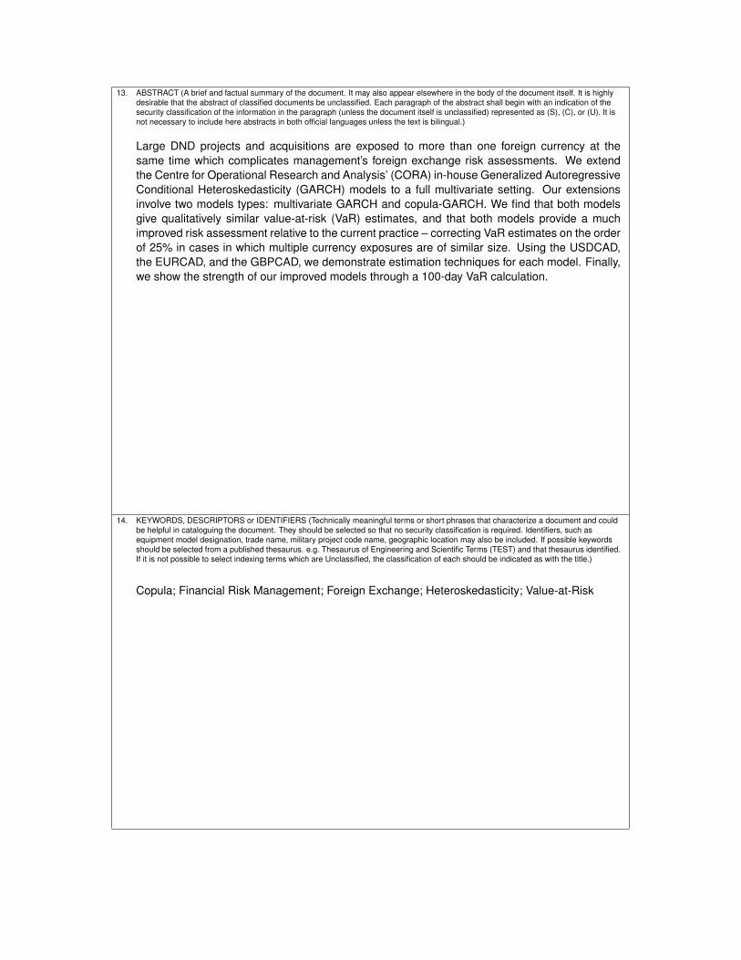
Large DND projects and acquisitions are exposed to more than one foreign currency at thesame time which complicates management’s foreign exchange risk assessments. We extendthe Centre for Operational Research and Analysis’ (CORA) in-house Generalized AutoregressiveConditional Heteroskedasticity (GARCH) models to a full multivariate setting. Our extensionsinvolve two models types: multivariate GARCH and copula-GARCH. We find that both modelsgive qualitatively similar value-at-risk (VaR) estimates, and that both models provide a muchimproved risk assessment relative to the current practice – correcting VaR estimates on the orderof 25% in cases in which multiple currency exposures are of similar size. Using the USDCAD,the EURCAD, and the GBPCAD, we demonstrate estimation techniques for each model. Finally,we show the strength of our improved models through a 100-day VaR calculation.

14. KEYWORDS, DESCRIPTORS or IDENTIFIERS (Technically meaningful terms or short phrases that characterize a document and couldbe helpful in cataloguing the document. They should be selected so that no security classification is required. Identifiers, such asequipment model designation, trade name, military project code name, geographic location may also be included. If possible keywordsshould be selected from a published thesaurus. e.g. Thesaurus of Engineering and Scientific Terms (TEST) and that thesaurus identified.If it is not possible to select indexing terms which are Unclassified, the classification of each should be indicated as with the title.)

Copula; Financial Risk Management; Foreign Exchange; Heteroskedasticity; Value-at-Risk

www.drdc-rddc.gc.ca

foreign exchange value-at-risk with multiple currency exposure · foreign exchange value-at-risk...

Documents