foreign threat and economic growth - rieti · foreign threat and economic growth* hideaki murase**,...

Foreign Threat and Economic Growth*

Hideaki Murase**, Hideki Toya***, and Di Zhao****

September 2010

Abstract

This paper offers a theoretical model and empirical evidence on the effects of threats of foreign invasion on the threatened country’s economic growth. In the model, the government controlled by the elite who hold an encompassing power has an incentive to be developmental. However, development increases the masses’ ability to contest power and hence the incentive is constrained by the elite’s fear of losing power. Under this circumstance, threats of foreign invasion may relax the constraint and allow the government to be more developmental since they may decrease the masses’ willingness to contest power, i.e., foreign countries can play a role of the common enemy, which enhances the “cooperation” between the elite and the masses. Our empirical evidence validates this prediction of the model: an increase in threats of foreign invasion significantly increases the growth rate of the threatened country through an increase in its human capital and TFP. Specifically, it significantly affects the composition of government expenditures, i.e., it increases education and investment expenditures but decreases consumption expenditure, with the total size of government expenditures unchanged. Keywords: Economic growth; Invasion; Revolution; Endogenous policy JEL Classification: D72; D74; D78; O10; O57 * We thank Kazumi Asako, Juro Teranishi, Masaya Sakuragawa, Mototsugu Fukushige, Masayuski Otaki, Moriki Hosoe, seminar participants at the Institute of Economic Research of Kyoto University, Keio University, Nihon University and Nagoya Gakuin University, and participants at the 2010 Spring Meeting of Japan Association for Applied Economics for their helpful comments. ** Faculty of Economics, Nagoya City University, Yamanohata Mizuho-cho

Mizuho-ku Nagoya, 467-8501, Japan. Tel&Fax:+81 52 872 5740; E-mail: [email protected]

*** Faculty of Economics, Nagoya City University **** Graduate School of Economics, Nagoya City University

1

1. Introduction

To explain the cross-country difference in economic growth, the recent literature has emphasized the role of government policies played in fostering or hindering development. However, if policies play a crucial role in determining each country’s growth performance, a deeper question is: why all countries do not adopt policies good for development. The simplest answer is that, in poor countries, non-democratic governments pursue inefficient policies to maximize the welfare of the dictator, autocrats, or more broadly ruling elites, which differ from the efficient policies to maximize national product or social welfare. While this answer seems plausible, the rational choice theory predicts the opposite, i.e., since non-democratic regimes controlled by the politically powerful elite would be a self-serving system, the elite could have a strong incentive to promote development and to extract sufficient fruits from the resulting prosperity. Specifically, if the elite have a large enough encompassing interest in the economy, they may be strongly motivated to adopt the efficient policies (see Olson, 1982; 1993 and McGuire and Olson, 1996).1

The recent research has attempted to fill this gap between theory and reality. Acemoglu and Robinson (2000, 2006) and Robinson (2001) develop a theory to explain why the elite cannot extract enough resources from the rest of the economy and, as a result, fail to adopt the efficient policies (see also Robinson, 1998). They argue that development tends to be inconsistent with the maintenance of the political status quo, and thereby the elite’s incentive to promote development is constrained by their fear of losing political power. This “political constraint” can be thought of as a particular form of contractual incompleteness in politics, which may deter the adoption of the efficient policies by the government (see North, 1981). Specifically, due to this “political constraint”, the elite may confront the trade-off between an increase in economic rent and a decrease in political power and, if the elite face a tighter constraint, they are more prone to adopt inefficient policies in

1 This incentive of non-democratic governments is often thought of as analogous to that of firm owners. That is, as the residual claimants on national product, they do not wish to “kill the goose that laid the golden egg”.

2

order to maintain their current political power.2 This paper focuses on threats of foreign invasion as a critical political

factor which may affect the tightness of the “political constraint” in non-democratic countries. Specifically, we offer a simple model to discuss how this geopolitical factor can influence the government’s incentive for development, policies, and economic growth. The crucial point is that, in the context of the conflict between the elite and the masses, an additional conflict of foreign invasion may decrease the masses’ willingness to contest power and hence relax the “political constraint” on the elite. This may occur because foreign countries play a role of the common enemy leading to a more congruence of interest between the elite and the masses in the domestic country. Specifically, domestic political stability may help the victory in an international conflict and hence benefit not only the elite but the masses as well. As a result, under an increase in threats of foreign invasion, the masses more restrain themselves from contesting power and the elite can pursue more development, although development may increase the masses’’ ability to contest power.

We also perform empirical research into this relation between foreign threat and economic growth, using a newly constructed index of each country’s political instability. Our index of political instability is the weighted sum of number of international conflicts that foreign countries have engaged in (the weight is given by the inverse of the domestic country’s distance from each international conflict). We use this index as a proxy for the amount of threats of foreign invasion perceived by the domestic country, assuming that the domestic country is more likely to be threatened by

2 This “political constraint” can also be thought of as one of the causes for the failure of the “political Coase theorem” that asserts the irrelevance of political regimes (i.e., who has political power) to economic efficiency. For instance, if non-democratic governments can gain less political legitimacy due to the limited people’s participation in political process than democratic ones, the constraint may be more significant for the former. Hence, according to the degree of constraint tightness, the adopted policies (and hence growth performance) may be more diverse among non-democratic countries than among democratic ones; see, for further discussion on (the failure of) the “political Coase theorem”, Acemoglu (2003).

3

foreign invasion as neighboring countries have more often engaged in international conflicts. One important advantage of our index is its relative exogeneity in growth regressions, i.e., the number of international conflicts that foreign countries have engaged in is admittedly external to the domestic country’s economic and political conditions. Thus, our findings are less subject to the usual causality problem that political instability, policies, and economic growth are jointly determined variables.

Our estimation results strongly support the model predictions. That is, an increase in threats of foreign invasion significantly increases the growth rate of the threatened country. Our results also show that this occurs through an increase in its human capital and TFP. Specifically, an increase in foreign threat significantly affects the composition of government expenditures, i.e., it increases the education and investment expenditures but decreases the consumption expenditure, with the total size of government expenditures unchanged. Furthermore, we find that these results are particularly true for non-democratic countries rather than for democratic ones, although the political regime itself has no direct relation to the country’s economic growth or the composition of government expenditures. Hence, our evidence suggests that what matters in determining each country’s growth performance is not the political regime itself, but the “political constraint” which may be more significant for non-democratic regimes facing more substantial domestic conflicts between the elite and the masses.

From the historical perspective, there are several examples of development motivated by threats of foreign invasion. For example, after the defeat in the Crimean War, Russia initiated a large-scale investment in infrastructure in order to modernize its economy, recognizing its vulnerability to foreign threat. Japan in the 19th century, facing the threat of being colonized by the European powers, spurred rapid industrialization. Similarly, Turkey threatened by foreign invasion after the decline of the Ottoman Empire attempted to industrialize its economy and moreover to democratize its political system. The most prominent examples after World War II may be Asian developmental dictatorships such as Taiwan under Chiang Kai Shek and South Korea under Park Chung Hee, which faced the threats of communist invasion. Our empirical evidence may demonstrate that this phenomenon of development motivated by foreign threat is not

4

limited to that of historical episodes, but is a general tendency prevailing in the modern world.

There are several theoretical and empirical studies closely related to ours. On the theoretical side, Acemoglu and Robinson (2006) and Chaudhry and Garner (2006) present models which relate an increase in threats of international conflict to a higher economic growth of the threatened country. Their model formulation is based on the notion that a more productive country is more advantageous in an international conflict. Thus, in their models, facing foreign threat, the elite pursue development in order to hold a dominant position in an international conflict, while taking a risk of an escalating domestic conflict. Our model formulation is based on a slightly different notion. Facing foreign threat, the masses adopt a more cooperative attitude toward the regime since they share common interests with the elite in an international conflict. Hence, the elite are allowed to pursue development, facing a relatively low risk of an escalating domestic conflict. Our formulation partially reflects the experience of Japan in the 19th century. That is, after the short-term civil war between competing military oligarchies, the Japanese autocracy had been quite stable until its defeat in World War II. This stability might be produced partly because the Japanese autocracy successfully established a strong centralized government in the early phase of industrialization, but at the same time the stability might be maintained because foreign threat harmonized the potentially conflicting interests of the elite and the masses in the Japanese autocracy. In contrast to this Japanese case, in Russia, rapid industrialization actually destabilized the elite’s political power and the regime was finally overthrown by the socialist revolution. Thus, the Russian case seems to be better captured by the notion of Acemoglu and Robinson (2006) and Chaudhry and Garner (2006), while the Japanese case seems to be better described by our notion. In reality, both mechanisms may work, perhaps simultaneously. Hence, we believe that their models and ours are not mutually exclusive but complementary.

On the empirical side, using the number of political assassinations, revolutions and coups as the index of political instability, Barro (1991) demonstrates that each country’s growth performance negatively depends on these political instability variables. Alesina, Ozler, Roubini, and Swagel (1996), using other variables of political instability, reach the same

5

conclusion. Benhabib and Spiegel (1992) and Alesina and Perotti (1993) find evidence that political instability impedes investment. Among others, Ades and Chua (1997) is closest to our paper in that they focus on the international spillovers of effects of political instability. They provide evidence that political instability in neighboring countries (measured by the number of revolutions and coups) has a negative impact on the growth performance of a domestic country. At first glance, the result of Ades and Chua (1997) which discovers negative spillovers of regional instability contrasts with our result. However, it is consistent with our model prediction, i.e., political instability in neighboring countries reduces their “national power” and mitigates foreign threat upon the domestic country, which in turn hinders the development incentive of the domestic government. The result of Easterly and Levine (1998) that the poor economic performance of neighboring countries negatively affects the income level of a domestic country could be reinterpreted in a similar vein.

The rest of the paper is organized as follows. The next section offers the theoretical model which discusses a possible mechanism in which an increase in threats of foreign invasion can lead to a higher economic growth of the threatened country. Section 3 explains the data used in the empirical analysis. Section 4 presents empirical evidence that validates the prediction of the model. Section 5 concludes the paper.

2. The model

This section presents a simple model to illustrate a possible mechanism relating an increase in threats of foreign invasion to a higher growth of the threatened country. To explain the basic structure of the model, we first consider the country under no threats of foreign invasion. Then, we add the possibility of foreign invasion to the model and discuss how it affects the threatened country’s growth.

6

2.1. No threats of foreign invasion Population

Consider an infinite horizon economy in discrete time. The economy consists of the masses and the ruling elite. The political regime is non-democratic, in which the government is controlled by the ruling elite. Each agent lives for one period and bears one child at the time of his/her death. Hence, generations do not overlap and the size of population remains constant over time. The membership of two groups, the masses and the elite, is assumed to be exogenous, i.e., the children of the masses (the elite) become the masses (the elite). Further, without loss of generality, the size of agents in each group is normalized to 1.

Preference The elite have preference over consumption and bequest. The

preference of each agent belonging to the elite group is given by:

11

1( , ) ( ) ( )

(1 )e e e e e et t t t tU U c w c w

, (1)

where etc is her consumption, e

tw is her bequest, and is a constant with

0 1 (the subscript denotes time throughout the paper). Meanwhile, the

masses have preference over consumption. The preference of each agent belonging to the mass group is given by:

( )m m m mt t tU U c c , (2)

where mtc is his consumption.3 Note that the preferences given by (1) and

3 In our model, what matters is that the bequest motive of the elite is stronger than that of the masses. Hence, we could alternatively formulate

the masses’ preference as 11

1( , ) ( ) ( )

(1 )m m m m m mt t t t tU U c w c w

, where

mtw is the masses’ bequest and is a constant with 0 . However,

7

(2) are linear (risk-neutral) in terms of income; specifically, the expected utility of each agent coincides with his/her expected income.

Production The economy produces a single good using the masses’ labor.

Specifically, the good is produced by the following linear technology:

( ) mt t tY A G L , (3)

where tY is the produced good, mtL is the masses’ labor devoted to the good

production, and ( )tA G is the productivity of the masses’ labor. tG is the

government investment in the public infrastructure and/or public education, which increase the productivity of the masses’ labor. In the below, we simply call tG as the “investment” and assume that ( )t tA G AG , where A is a

positive constant. We also assume that the elite do not engage in the good production, but only engage in the government activity, especially the maintenance of the existing order such as policing.

Government policies In the existing order, political power to decide public policies is monopolized by the elite. However, the masses have a potential to attempt a revolution, the success of which allows the masses to take political power from the elite. There are two public policies: investment policy and taxation policy. The investment policy determines the productivity of the masses’ labor. Specifically, at the beginning of each period, the government implements the investment policy that allocates the fraction of the elite’s inherited bequest to the “investment”. We denote this fraction by t ( 0 1t ). The remaining

fraction of the elite’s inherited bequest is used for the government activity that the elite engage in, and determines its productivity. In the below, we simply call the productivity of the government activity as the “productivity of the elite” and denote it by tD . Given this investment policy, the productivity

this formulation would complicate the analysis but add little insight.

8

of the masses and that of the elite are assumed to be given by 1e

t t tG w and

1(1 ) et t tD w respectively. 4 The taxation policy, on the other hand,

determines the allocation of the produced good between the masses and the elite. Specifically, after implementing the investment policy, the government decides the tax rate imposed on the produced good. We assume that this tax rate denoted by *t is applied only in the case where no revolution is

attempted; the tax rate in the case where a revolution occurs will be discussed below. Letting t (0 1t ) be the tax rate, we obtain the income of the masses and that of the elite as (1 )t tY and t tY respectively. This

formulation of the taxation policy implies that the income of the elite is a pure rent and t parameterizes the elite’s encompassing power.

Revolution (Domestic conflict) Now consider a revolution, which is the masses’ activity with the aim of taking political power from the elite. If a revolution is initiated, it succeeds with probability tp and fails with probability 1 tp ( 0 1tp ). The

government investment in public infrastructure and/or public education increases the masses’ ability to contest power and destabilizes the elite’s political power. To capture this notion, we assume that the larger the productivity of the masses relative to that of the elite, the larger the success probability of revolution. Specifically, the success probability takes a form of the contest success function introduced by Tullock (1967, 1980) for the analysis of rent-seeking contests:5

tt t

t t

Gp

G D

. (4)

If a revolution is initiated, it absorbs human resources. Specifically, it

absorbs the fraction (1 ) of labor of the masses and that of elite. Hence,

4 For simplicity, tG and tD last for one period and completely depreciate

at the end of each period. 5 See also Grossman (1991, 1994) and Skaperdas (1992) for the contest success functions used in conflict literature.

9

the masses’ labor devoted to good production decreases from 1mtL to

mtL when a revolution is initiated. For the convenience of the analysis

below, we assume that 1

12

. Further, we assume that the initial taxation

policy decided by the government is abolished if a revolution is attempted. Without loss of generality, we assume a-winner-takes-all situation: when a revolution succeeds, the masses remove the elite from political power and set the lowest possible tax rate, i.e., 0t ; when it fails, the elite set the highest possible tax rate, i.e., 1t . Given these tax rates, the income (the utility) of

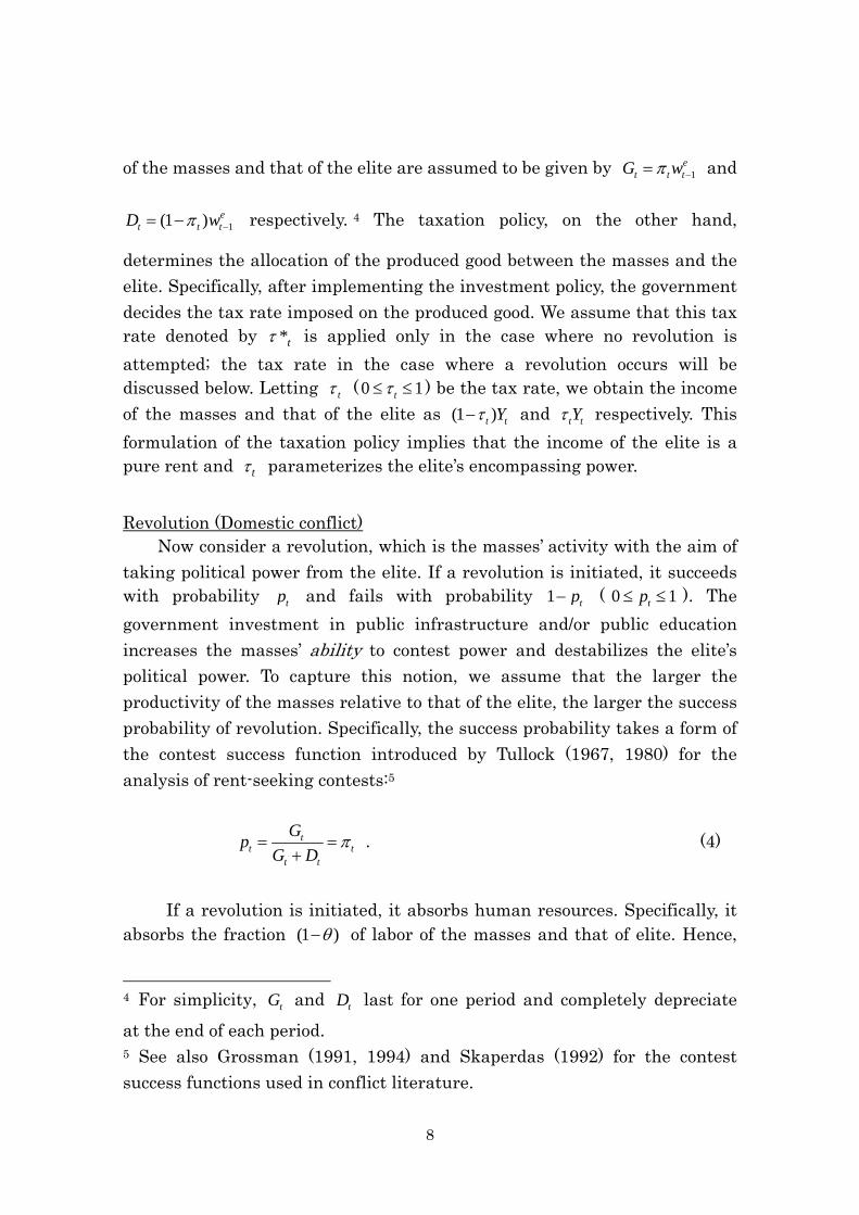
each group is summarized in the “game-tree” depicted in Figure 1. Economic growth

We first examine the within-a-period equilibrium by working backward and then compute the equilibrium growth rate. Recalling that the preference of each agent is linear in terms of his /her income, we obtain the masses’ expected utility as:

(1 * ) 0

1t t tm

tt t t

AG ifU

p AG if

, (5)

where t is the index variable that takes on 1 if the masses attempt a

revolution; 0 otherwise. The masses attempt a revolution when they find it profitable. Thus, from (5), the index variable t is determined as:

1 *0

1 *1t t

tt t

pif

pif

. (6)

Eq. (6) can be thought of as a “reaction function” that describes the masses’ political response to the tax rate that the government decides. Next, the expected utility of the elite is given by:

10

* 0

(1 ) 1t t te

tt t t

AG ifU

p AG if

. (7)

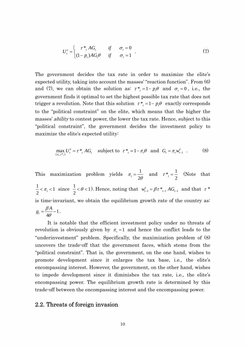
The government decides the tax rate in order to maximize the elite’s expected utility, taking into account the masses’ “reaction function”. From (6) and (7), we can obtain the solution as: * 1t tp and 0t , i.e., the

government finds it optimal to set the highest possible tax rate that does not trigger a revolution. Note that this solution * 1t tp exactly corresponds

to the “political constraint” on the elite, which means that the higher the masses’ ability to contest power, the lower the tax rate. Hence, subject to this “political constraint”, the government decides the investment policy to maximize the elite’s expected utility:

{ , * }max *

t t

et t tU AG

subject to * 1t t and 1

et t tG w . (8)

This maximization problem yields 1

2t and

1*

2t (Note that

11

2 t since 1

12

). Hence, noting that 1 1 1*et t tw AG and that *

is time-invariant, we obtain the equilibrium growth rate of the country as:

14t

Ag

.

It is notable that the efficient investment policy under no threats of revolution is obviously given by 1t and hence the conflict leads to the

“underinvestment” problem. Specifically, the maximization problem of (8) uncovers the trade-off that the government faces, which stems from the “political constraint”. That is, the government, on the one hand, wishes to promote development since it enlarges the tax base, i.e., the elite’s encompassing interest. However, the government, on the other hand, wishes to impede development since it diminishes the tax rate, i.e., the elite’s encompassing power. The equilibrium growth rate is determined by this trade-off between the encompassing interest and the encompassing power.

2.2. Threats of foreign invasion

11

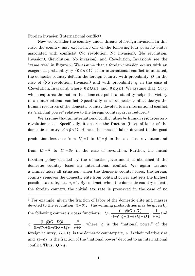
Foreign invasion (International conflict) Now we consider the country under threats of foreign invasion. In this

case, the country may experience one of the following four possible states associated with conflicts: (No revolution, No invasion), (No revolution, Invasion), (Revolution, No invasion), and (Revolution, Invasion); see the “game-tree” in Figure 2. We assume that a foreign invasion occurs with an exogenous probability ( 0 1 ). If an international conflict is initiated, the domestic country defeats the foreign country with probability Q in the case of (No revolution, Invasion) and with probability q in the case of (Revolution, Invasion), where 0 1Q and 0 1q . We assume that Q q ,

which captures the notion that domestic political stability helps the victory in an international conflict. Specifically, since domestic conflict decays the human resources of the domestic country devoted to an international conflict, its “national power” relative to the foreign counterpart is reduced.6

We assume that an international conflict absorbs human resources as a revolution does. Specifically, it absorbs the fraction (1 ) of labor of the domestic country ( 0 1 ). Hence, the masses’ labor devoted to the good

production decreases from 1mtL to m

tL in the case of no revolution and

from mtL to m

tL in the case of revolution. Further, the initial

taxation policy decided by the domestic government is abolished if the domestic country loses an international conflict. We again assume a-winner-takes-all situation: when the domestic country loses, the foreign country removes the domestic elite from political power and sets the highest possible tax rate, i.e., 1t . By contrast, when the domestic country defeats

the foreign country, the initial tax rate is preserved in the case of no 6 For example, given the fraction of labor of the domestic elite and masses devoted to the revolution (1 ) , the winning probabilities may be given by

the following contest success functions: (1 )( ) 1

(1 ) (1 )( ) 1t t

t t t

G DQ

V G D

and

(1 )( )

(1 ) (1 )( )t t

t t t

G Dq

V G D

, where tV is the “national power” of the

foreign country, t tG D is the domestic counterpart, is their relative size,

and (1 ) is the fraction of the “national power” devoted to an international conflict. Thus, Q q .

12

revolution, i.e., *t t , while 0t in the case of successful revolution and 1t in the case of failed revolution. Hence, given these tax rates, the utility

of each group is summarized as in the “game-tree” in Figure 2. Economic growth

Let us turn to the equilibrium growth rate in the presence of foreign threat. First, the masses’ expected utility is given by:

( 1 )(1 * ) 0

( 1 ) 1t t tm

tt t t

Q AG ifU

q p AG if

, (9)

Then, the index variable t that indicates whether a revolution is

attempted or not can be obtained as:

1 ( , ; , ) *0

1 ( , ; , ) *1t t

tt t

Q q pif

Q q pif

, (10)

where 1

( , ; , )1

qQ q

Q

; note that 1 and 0

. Meanwhile,

the expected utility of the elite is given by:

( 1 ) * 0

( 1 )(1 ) 1t t tg

tt t t

Q AG ifU

q p AG if

. (11)

As in the case of no threats of foreign invasion, the government decides the tax rate in order to maximize the elite’s expected utility, taking into account the masses’ “reaction function” (10). Again, the optimal tax rate is obtained as the highest possible one that does not trigger a revolution, i.e.,

* 1 ( , ; , )t tp Q q and 0t . Note that, compared with the case of no

threats of foreign invasion, the “political constraint” may be more relaxed in the presence of foreign threat since 1 . This is because the defeat in an international conflict harms not only the elite but the masses as well and the masses more restrain themselves from attempting a revolution. Hence, in the presence of foreign threat, the government can decide the investment

13

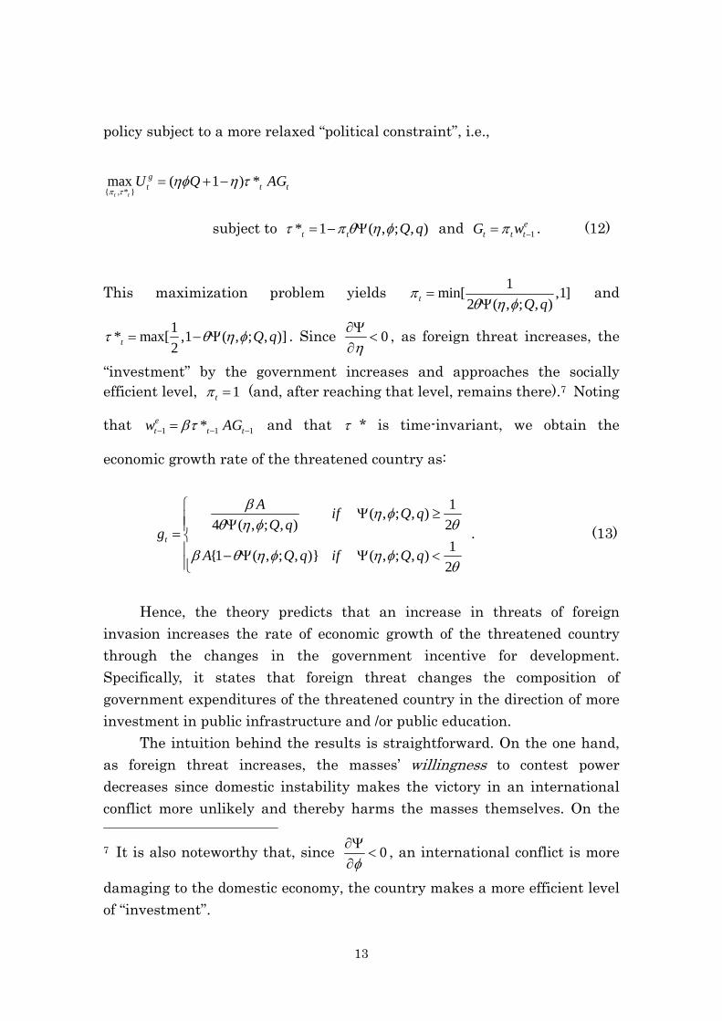
policy subject to a more relaxed “political constraint”, i.e.,

{ , * }max ( 1 ) *

t t

gt t tU Q AG

subject to * 1 ( , ; , )t t Q q and 1e

t t tG w . (12)

This maximization problem yields 1

min[ ,1]2 ( , ; , )t Q q

and

1* max[ ,1 ( , ; , )]

2t Q q . Since 0

, as foreign threat increases, the

“investment” by the government increases and approaches the socially efficient level, 1t (and, after reaching that level, remains there).7 Noting

that 1 1 1*et t tw AG and that * is time-invariant, we obtain the

economic growth rate of the threatened country as:

1( , ; , )

4 ( , ; , ) 2

1{1 ( , ; , )} ( , ; , )

2

t

Aif Q q

Q qg

A Q q if Q q

. (13)

Hence, the theory predicts that an increase in threats of foreign

invasion increases the rate of economic growth of the threatened country through the changes in the government incentive for development. Specifically, it states that foreign threat changes the composition of government expenditures of the threatened country in the direction of more investment in public infrastructure and /or public education.

The intuition behind the results is straightforward. On the one hand, as foreign threat increases, the masses’ willingness to contest power decreases since domestic instability makes the victory in an international conflict more unlikely and thereby harms the masses themselves. On the

7 It is also noteworthy that, since 0

, an international conflict is more

damaging to the domestic economy, the country makes a more efficient level of “investment”.

14

other hand, this decrease in the willingness to contest power may relax the “political constraint” on the elite, and the government can make more “investment”, although it increases the masses’ ability to contest power. In other words, foreign countries can play a role of the common enemy to alleviate the potential conflict of interests between the elite and the masses of the threatened country and enhance their “cooperation” in favor of economic growth.

3. The data To examine whether or not our model predictions are consistent with the actual data, we perform growth regressions using the cross-country data for the period 1960-1990. Appendix A provides the list of the countries used as the sample. We perform the cross-country regressions with special focus on the geopolitical condition that each country faces. For this purpose, we construct two new variables representing political instability of each country. The first variable is the index of threats of foreign invasion (hereafter called as TFI) which is given by:

i

Number of international conflicts Country j has engaged in TFI log

Distance from Country i to Country jj i

We use this index as a proxy for the potential foreign threat for Country i. Specifically, we assume that Country i is more likely to be threatened by foreign invasion as neighboring countries have more often engaged in international conflicts. Note also that the index is constructed as the sum of number of other countries’ international conflicts weighted by each country’s distance from those conflicts. Thus, we are here focusing on the “relative geography” variable which specifies each country’s situation on the globe

15

vis-a-vis other countries.8 The second variable is the index of domestic and international conflicts which each country has actually engaged in (hereafter called as WAR). This index is given by:

iWAR log(Number of domestic and international conflicts Country i has engaged in)

We use this index to control for the effects of domestic and international conflicts which Country i has engaged in on the country itself. Hence, what the two instability variables indicate are clearly separated, i.e., TFIi captures the potential “threats” of conflicts to Country i, while WARi captures the “outbreaks” of conflicts and the resultant physical and human damages to Country i. In our growth regressions, we also control for a lot of other variables considered as important determinants of economic growth in previous research. These variables are constructed from several different data sources. Appendix B summarizes the list of variables and the data source associated with each variable. Appendix C provides the summary statistics of all variables.

4. Empirical evidence

This section presents our empirical results concerning the effects of threats of foreign invasion and other variables on per capita GDP growth and the composition of government expenditures. We estimate all the regressions using an ordinary least squares procedure with the White’s

8 By contrast, the “absolute geography”, which is independent of the location and situation of other countries, refers to purely physical geography such as each country’s own climate and its own access to the sea; see Krugman (1993), Redding and Venables (2004) and Bosker and Garretsen (2008) for the distinction between the “absolute geography” and the “relative geography”.

16

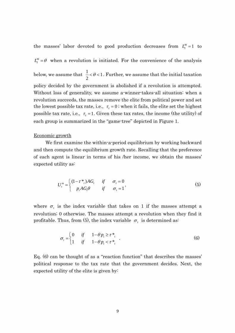
heteroskedasticity-consistent covariance matrix. Table 1 shows the basic regression results concerning the effects of threats of foreign invasion and other variables on per capita GDP growth. Column 1 reports the benchmark regression including TFI (the index of threats of foreign invasion) and controlling for initial GDP per capita and initial total schooling years. The regression result indicates that the coefficient of TFI is positive and highly significant, while that of WAR is negative and its magnitude is relatively small (Figure 3 depicts the partial relationship between TFI and per capita GDP growth obtained in Column 1). In Column 2, we control for other variables which previous research has recognized as important determinants of economic growth, i.e., population growth, investment, and openness. The result is mostly unchanged from Column 1, i.e., the coefficient of TFI remains significantly positive, while that of WAR is negative and becomes insignificant. Further, it might be suspected that FTI and WAR merely capture the effects of political regimes and thereby affect economic growth. To examine this point, we include the index of political regimes, Autocracy, of Glaezer et al. (2004) in Column 3. We again obtain a similar regression result associated with TFI and WAR. In addition, we find that the coefficient of Autocracy is negative but insignificant, which implies that there is no systematic difference in growth performance between non-democratic countries and democratic ones.

It is widely recognized that the economic growth of each country is driven by its physical capital accumulation, human capital accumulation, and productivity growth. Hence, we next include the variables associated with these factor accumulations into our regressions in order to examine the channels through which TFI has a positive impact on economic growth. Table 2 reports the results of the regressions controlling for the factor accumulations. Columns 1-3 show that, when we include physical capital accumulation, human capital accumulation, and productivity growth into the regressions, the impact of TFI on economic growth captured by its significance and magnitude of the coefficients is weakened. Then, as shown in Column 4, when all these factor accumulation variables are included, the impact of FTI becomes insignificant. These results strongly indicate that TFI has a positive impact on economic growth through the channel of enhancing these factor accumulations. Given the results obtained in Table 2, we proceed to examine whether

17

or not TFI actually stimulates factor accumulations. Table 3 reports the regression results which indicate that TFI is positively related to all the factor accumulation variables, while WAR is not. These results are consistent with our model prediction that foreign threat has a positive impact on factor accumulations by stimulating the government “investment” in public infrastructure and/or public education.

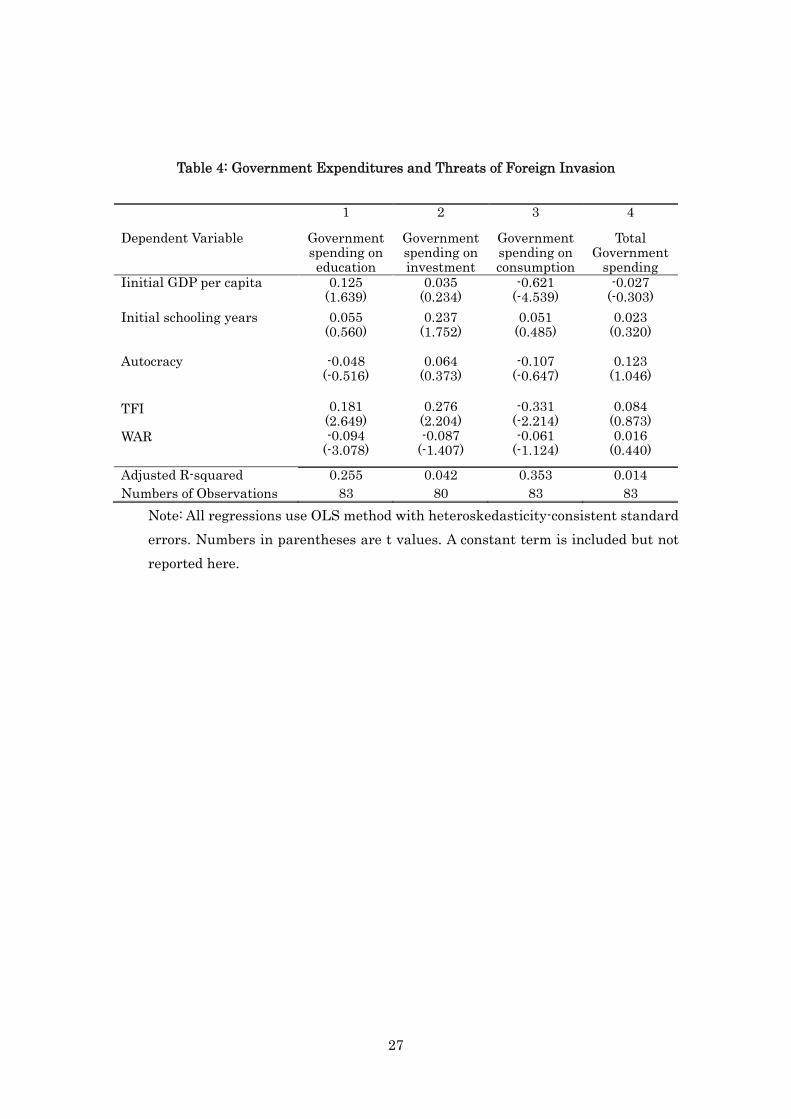
In order to more closely inspect this point, we perform the regressions concerning the effects of foreign thereat on government expenditures. Table 4 shows that TFI has a positive and significant impact on the government education and investment expenditures, while a negative and significant impact on the government consumption expenditure. Furthermore, it shows that TFI has no significant impact on the government size. These results are consistent with our model prediction, i.e., confronting with an increase in foreign threat, the composition of the government expenditures is changed in the direction of more “investment” and less “consumption”. Further, in all columns, we find that the coefficients on Autocracy are insignificant, which implies that political regime has no systematic effects on the composition of government expenditures.

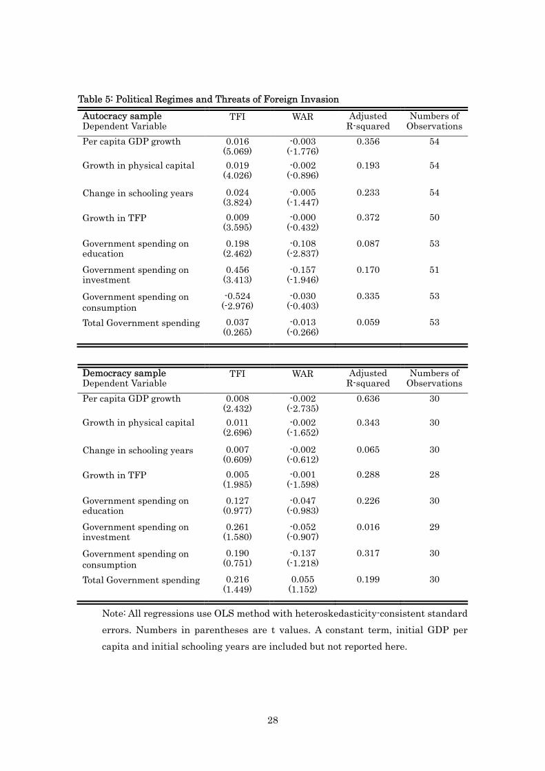
Tables 1 and 4 demonstrate that political regime itself has no direct impact on economic growth and the composition of government expenditures. However, the “political constraint” may be more significant for non-democratic countries than for democratic ones since the former can be thought of as facing more substantial domestic conflicts between the elite and the masses. Hence, the effects of foreign threat on economic growth may larger for non-democratic countries than for democratic ones. In order to examine whether or not such a difference across political regimes exists, we divide the sample countries into two sub-samples, i.e., the autocracy sample and the democracy sample. Table 5 reports the regression results for both sub-samples. They show that the effects of FTI on economic growth, factor accumulations, and government expenditures are all larger for the autocracy sample than for the democracy sample, both in their significance and magnitude. This result can be interpreted as evidence that what matters in determining the government incentive for development is not a political regime itself, but the “political constraint” that each government faces. That is, foreign threat may more relax the “political constraint” in non-democratic countries which face more substantial domestic political conflicts than

18

democratic ones.

5. Conclusion This paper has offered a theoretical model and empirical evidence on the effects of threats of foreign invasion on the threatened country’s economic growth. In the model, we show that in non-democratic countries foreign threat may decrease the masses’ willingness to contest power, relax the “political constraint” on the political elite, and allows the government to pursue more development although it increases the masses’ ability to contest power.

Our empirical results validate this prediction of the model. We find a significantly positive influence of threats of foreign invasion on the growth rate of the threatened country. We also find that this increase in the growth rate occurs through the increase in the threatened country’s human capital and TFP. Specifically, foreign threat significantly increases the government education and investment expenditures but decreases the government consumption expenditure, while the total size of expenditures remains unchanged. Furthermore, these results are particularly true for non-democratic countries rather than for democratic ones. Our theoretical and empirical results suggest that each country’s economic growth is not an economic event isolated from the rest of the world, but it is greatly influenced by political events taking place in the rest of the world. Specifically, our results indicate that the geopolitics surrounding each country, together with its own domestic politics, may be one of the deep determinants of the country’s policies and growth performance.

19

References

Acemoglu, D. (2003) “Why not a Political Coase Theorem? Social Conflict, Commitment, and Politics”, Journal of Comparative Economics 31:620-652.

Acemoglu, D., Robinson, J. A. (2000) “Political Losers as a Barrier to Economic Development”, American Economic Review 90: 126-130.

Acemoglu, D., Robinson, J. A. (2006) “Economic Backwardness in Political Perspective”, American Political Science Review 100: 115-131.

Ades, A., Chua, H. B. (1997) “Thy Neighbor’s Curse: Regional Instability and Economic Growth”, Journal of Economic Growth 2: 279-304.

Barro, R. J. (1991) “Economic Growth in a Cross Section of Countries” Quarterly Journal of Economics 106: 407-443.

Barro, R. J., Lee, J. W. (1994) Data Set for a Panel of 138 Countries. NBER. Available online at: http://www.nber.org/pub/barro.lee/readme.txt.

Barro, R. J. Lee. J. W. (2000) “International Data on Educational Attainment: Updates Implications”, CID Working Paper, No. 42.

Benhabib, J. Spiegel, M. M. (2002) “Human Capital and Technology Diffusion”, FRBSF Working Paper, 2.

Bosker, M., Garretsen, H. (2009) “Economic Development and the Geography of Institutions”, Journal of Economic Geography 9: 295-358.

Chaudhry, A., Phillip, G. (2006) “Political Competition between Countries and Economic Growth”, Review of Development Economics 10: 666-682.

CEPII Geographical Distances Data Set. Available online at: http://www.cepii.fr/distance/geo_cepii.xls.

Easterly, W., Levine, R. (1998) “Troubles with the Neighbors: Africa’s Problem, Africa’s Opportunity”, Journal of African Economics 7: 120-142.

Easterly, W., Levine, R. (2001) “It’s not Factor Accumulation: Stylized Facts and Growth Models”, World Bank Economic Review 15: 177-219.

Laporta G. E., Lopes-de-Silanes R., Shleifer, A. (2004) “Do Institutions Cause Growth?”, Journal of Economic Growth 9: 271-303.

Grossman, H. I. (1991) “A General Equilibrium Theory of Insurrections”, American Economic Review 81: 912-921.

Grossman, H. I. (1993) “Production, Appropriation and Land Reform”, American Economic Review 84: 705-712.

Krugman, P. (1993) “First Nature, Second Nature, and Metropolitan Location”, Journal of Regional Economics 33:129-144.

20

McGuire, M. C., Olson, M. (1996) “The Economics of Autocracy and Majority Rule”, Journal of Economic Literature 34: 72-96.

North, D. (1981) Structure and Change in Economic History. Norton: New York.

Olson, M. (1982) The Rise and Decline of Nations. Yale University Press: New Haven, CT.

Olson, M. (1993) “Dictatorship, Democracy and Development”, American Political Science Review 87: 567-576.

Redding, S., Venables, A. J. (2004) “Economic Geography and International Inequality”, Journal of International Economics 62: 53-82.

Robinson, J. A. (2001) “When is a State Predatory?”, Unpublished, Department of Government, Harvard University

Robinson, J. A. (1998) “Theories of Bad Policy”, Journal of Policy Reform 2:1-46.

Skaperdas, S. (1992) “Cooperation, Conflict, and Power in the Absence of Property Rights”, American Economic Review 82: 720-739.

Tullock, G. (1967) “The Welfare Costs of Tariffs, Monopolies and Theft”, Western Economic Journal 5: 224-232.

Tullock, G. (1980) “Efficient Rent Seeking”, In: Buchanan, J.M., Tollison, R.D., Tullock, G. (eds.) Toward a Theory of the Rent-seeking Society. Texas A＆M University Press: College Station, pp.16-36.

UCDP/PRIO Armed Conflict data set (Version4-2008). Available online at: http://www.prio.no/CSCW/Dataset/Armed-Conflict/UCDP-PRIO/.

21

Figure 1. Payoffs under No Threats of Foreign Invasion

t *t

* , (1 * )t t t tAG AG

, 0tAG

0, tAG

Investment policy

Taxation policy

No revolution

Fail

Revolution

Succeed

Note : The first and second variables in each parenthesis denote the elite’s utility and the masses’ utility respectively.

22

Figure 2. Payoffs under Threats of Foreign Invasion

t

, 0tAG

0, tAG

Investment policy

Taxation policy

No revolutionNo invasion

* , (1 * )t t t tAG AG

*t

* , (1 * )t t t tAG AG

0, 0

, 0tAG

0, tAG

0, 0

0, 0

RevolutionInvasion

RevolutionNo invasion

No revolutionInvasion

FailWin

FailLose

SucceedWin

SucceedLose

Win

Lose

Fail

Succeed

Note: The first and second variables in each parenthesis denote the elite’s utility and the masses’ utility respectively.

23

Figure 3. The Partial Relation of Threats of Foreign Invasion and Economic Growth

24

Table 1: Growth and Threats of Foreign Invasion

Dependent Variable: Per capita GDP Growth

1 2 3 Initial GDP per capita -0.007

(-2.953) -0.009

(-3.517) -0.010

(-3.509) Initial schooling years 0.014

(6.476) 0.007

(3.535) 0.007

(3.393) Population growth -0.396

(-2.300) -0.361

(-1.935) Investment 0.014

(4.057) 0.014

(3.839) Openness -0.003

(-1.417) -0.003

(-1.378) Autocracy -0.002

(-1.378) TFI 0.015

(6.331) 0.010

(4.853) 0.011

(4.860) WAR -0.003

(-2.450) -0.002

(-1.566) -0.001

(-1.623)

Adjusted R-squared 0.419 0.505 0.502 Numbers of Observations 84 82 82

Note: All regressions use OLS method with heteroskedasticity-consistent standard

errors. Numbers in parentheses are t values. A constant term is included but not

reported here.

25

Table 2: Growth, Factor Accumulation, and Threats of Foreign Invasion

Dependent Variable: Per capita GDP Growth

1 2 3 4 Initial GDP per capita -0.002

(-1.057) -0.007

(-3.381) -0.002

(-1.501) -0.000

(-0.419) Initial schooling years 0.007

(3.421) 0.012

(6.384) 0.002

(1.353) 0.001

(0.821) Growth in physical capital 0.410

(6.660) 0.253

(7.068)

Change in schooling years 0.117(2.934)

-0.018(-0.926)

Growth in TFP 1.147(11.56)

0.873 (10.57)

TFI 0.007(3.012)

0.012(5.312)

0.005(4.166)

0.003 (1.316)

WAR -0.002(-2.520)

-0.002(-2.224)

-0.002(-3.837)

-0.000(-0.842)

Adjusted R-squared 0.682 0.465 0.812 0.890 Numbers of Observations 84 84 78 78



reported here.

26

Table 3 : Factor Accumulation and Threats of Foreign Invasion

1 2 3

Dependent Variable Growth in physical capital

Change in schooling

years

Growth in TFP

Initial GDP per capita -0.012(-3.126)

0.010(1.565)

-0.004 (-2.077)

Initial schooling years

0.015(4.249)

0.007(1.226)

0.009 (5.160)

TFI 0.016(4.354)

0.018(2.767)

0.007 (3.860)

WAR -0.002(-1.162)

-0.004(-1.431)

-0.000 (-0.388)

Adjusted R-squared 0.223 0.072 0.343 Numbers of Observations 84 84 78



reported here.

27

Table 4: Government Expenditures and Threats of Foreign Invasion

1 2 3 4

Dependent Variable Government spending on education

Government spending on investment

Government spending on consumption

Total Government

spending Iinitial GDP per capita 0.125

(1.639) 0.035

(0.234) -0.621

(-4.539) -0.027

(-0.303)

Initial schooling years Autocracy

0.055(0.560)

-0.048

(-0.516)

0.237(1.752)

0.064

(0.373)

0.051(0.485)

-0.107

(-0.647)

0.023 (0.320)

0.123

(1.046) TFI 0.181

(2.649) 0.276

(2.204) -0.331

(-2.214)

0.084

(0.873) WAR -0.094

(-3.078) -0.087

(-1.407) -0.061

(-1.124) 0.016

(0.440)

Adjusted R-squared 0.255 0.042 0.353 0.014 Numbers of Observations 83 80 83 83



reported here.

28

Table 5: Political Regimes and Threats of Foreign Invasion

Autocracy sampleDependent Variable

TFI WAR Adjusted R-squared

Numbers of Observations

Per capita GDP growth 0.016(5.069)

-0.003(-1.776)

0.356 54

Growth in physical capital 0.019(4.026)

-0.002(-0.896)

0.193 54


-0.005(-1.447)

0.233 54


-0.000(-0.432)

0.372 50

Government spending on education

0.198(2.462)

-0.108(-2.837)

0.087 53


0.456(3.413)

-0.157(-1.946)

0.170 51


-0.524(-2.976)

-0.030(-0.403)

0.335 53

Total Government spending 0.037(0.265)

-0.013(-0.266)

0.059 53

Democracy sampleDependent Variable

TFI WAR Adjusted R-squared

Numbers of Observations

Per capita GDP growth 0.008(2.432)

-0.002(-2.735)

0.636 30

Growth in physical capital 0.011(2.696)

-0.002(-1.652)

0.343 30


-0.002(-0.612)

0.065 30


-0.001(-1.598)

0.288 28


0.127(0.977)

-0.047(-0.983)

0.226 30


0.261(1.580)

-0.052(-0.907)

0.016 29


0.190(0.751)

-0.137(-1.218)

0.317 30

Total Government spending 0.216(1.449)

0.055(1.152)

0.199 30


errors. Numbers in parentheses are t values. A constant term, initial GDP per

capita and initial schooling years are included but not reported here.

29

Appendix A. List of Countries

Algeria A Honduras A Philippines A

Argentina A Iceland B Portugal A

Australia B India B Senegal A

Austria B Indonesia A Singapore A

Bangladesh A Iran A South Africa A

Barbados B Ireland B Spain A

Belgium B Israel B Sri Lanka A

Bolivia A Italy B Swaziland A

Botswana A Jamaica B Sweden B

Brazil A Japan B Switzerland B

Cameroon A Jordan A Syria A

Canada B Kenya A Taiwan A

Central African Rep. A Korea, Republic of A Thailand A

Chile A Lesotho A Togo A

Colombia B Malawi A Trinidad &Tobago B

Congo, Dem. Rep. A Malaysia A Tunisia A

Costa Rica B Mali A Turkey A

Denmark B Malta B Uganda A

Dominican Republic A Mauritius B United Kingdom B

Ecuador A Mexico A United States B

El Salvador A Mozambique A Uruguay A

Fiji A Netherlands B Venezuela B

Finland B New Zealand B Zambia A

France B Niger A Zimbabwe A

Germany B Norway B

Ghana A Pakistan A

Greece A Panama A

Guatemala A Papua New Guinea B

Guyana A Paraguay A

Haiti A Peru A

Note: A indicates that the country’s autocracy index is higher than zero. B indicates that

the country’s autocracy index is equal to zero.

30

Appendix B. Definition of Variables

Variable Variable Definition Source

TFI Logarithm of number of external wars in all foreign countries for the period 1960-1990, weighted by distance from the domestic country to each country

UCDP/PRIO & CEPII

WAR Logarithm of 1+numbers of internal and external wars in the domestic country for the period 1960-1990

UCDP/PRIO & CEPII

Per capita GDP growth Average growth rate of real per capita GDP for the period 1960-1989

Barro & Lee(1994)

Growth in physical capital Average growth rate of physical capital per capita for the period 1961-1989

Easterly & Levine (2001)

Change in schooling years Difference between average years of schooling in 1990 and average years of schooling in 1960

Barro & Lee(2000)

Growth in TFP Average growth rate of total factor productivity for the period 1960-1995

Benhabib & Spiegel(2003)

Initial GDP per capita Logarithm of initial real per capita GDP in1960

Barro & Lee(1994)

Initial schooling years Logarithm of initial average schooling years in total population over age 25 in1960

Barro & Lee(2000)

Population growth Average growth rate of population for the period 1960-1990

Penn World Table 6.3

Investment Logarithm of average ratio of real domestic investment to real GDP for the period 1960-1990

Barro & Lee(1994)

Openness Logarithm of average ratio of total trade value to GDP for the period 1960-1990

Barro & Lee(1994)

Autocracy Average index of autocracy for the period 1960-1990

Shleifer et al.(2004)


Logarithm of average ratio of nominal government education expenditure to nominal GDP for the period 1960-1985

Barro & Lee(1994)


Logarithm of average ratio of nominal government investment expenditure to nominal GDP for the period 1960-1985

Barro & Lee(1994)


Logarithm of average ratio of nominal government consumption expenditure to nominal GDP for the period 1960-1985

Barro & Lee(1994)

Total government spending Logarithm of average government share of real GDP per capita for the period 1960-1990

Penn World Table 6.3

31

Appendix C. Summary of Statistics

Variable Mean Standard Dev. Observations

TFI 1.594 0.557 84

WAR 1.067 1.259 84

Per capita GDP growth 0.021 0.016 84

Growth in physical capital 0.029 0.024 84

Change in schooling years 0.070 0.034 84

Growth in TFP 0.012 0.011 78

Initial GDP per capita 7.502 0.877 84

Initial schooling years 0.910 0.948 84

Population growth 0.019 0.009 84

Investment 2.872 0.535 84

Openness 3.421 0.695 82

Autocracy 0.675 0.576 84


1.294 0.402 83


1.636 0.614 80


1.995 0.733 83

Total government spending 2.929 0.381 83

foreign threat and economic growth - rieti · foreign threat and economic growth* hideaki murase**,...

Documents