forgetting the flood?: an analysis of the flood risk...

Forgetting the Flood?: An Analysis of the Flood Risk Discountover Time

Ajita Atreya, Susana Ferreira, Warren Kriesel

Land Economics, Volume 89, Number 4, November 2013, pp. 577-596 (Article)

Published by University of Wisconsin Press

For additional information about this article

Access provided by University Of Pennsylvania (4 Nov 2013 11:04 GMT)

http://muse.jhu.edu/journals/lde/summary/v089/89.4.atreya.html

http://muse.jhu.edu/journals/lde/summary/v089/89.4.atreya.html

Forgetting the Flood? An Analysis of the Flood RiskDiscount over Time

Ajita Atreya, Susana Ferreira, and Warren Kriesel

ABSTRACT. We examine whether property price dif-ferentials reflecting flood risk increase following alarge flood event, and whether this change is tempo-rary or permanent. We use single-family residentialproperty sales in Dougherty County, Georgia, be-tween 1985 and 2004 in a difference-in-differencesspatial hedonic model framework. After the 1994“flood of the century,” prices of properties in the 100-year floodplain fell significantly. This effect was, how-ever, short-lived. In spatial hedonic models that ex-plicitly incorporate both linear and nonlineartemporal flood-zone effects, we show that the floodrisk discount disappeared between four and nineyears after the flood, depending upon the specifica-tion. (JEL Q51, Q54)

I. INTRODUCTION

Floods are the most common natural disas-ter. Between 1985 and 2009, floods repre-sented 40% of all natural disasters worldwideand accounted for 13% of the deaths and 53%of the number of people affected by all naturaldisasters (CRED 2010).1 In the United States,floods kill about 140 people and cause $6 bil-lion in property damage in the average year(USGS 2006). Between 1955 and 2009, eco-nomic damages from flooding in the UnitedStates amounted to over $260 billion in con-stant 2009 dollars.

Flood damage has increased in the UnitedStates, despite local efforts and federal en-couragement to mitigate flood hazards andregulate development in flood-prone areas

1 To be considered a disaster and included in the widelyused EM-DAT global disaster database, an event needs tofulfill at least one of the following criteria: (1) 10 or morepeople killed, (2) 100 or more people reported affected (typ-ically displaced), (3) a declaration of a state of emergency,or (4) a call for international assistance (CRED 2010).

Land Economics • November 2013 • 89 (4): 577–596ISSN 0023-7639; E-ISSN 1543-8325� 2013 by the Board of Regents of theUniversity of Wisconsin System

(Pielke, Downton, and Miller 2002). IPCC(2001) and Swiss Re (2006) have reported asimilar trend across the world. The increaseddamages are believed to have two causes. Thefirst is an increase in the frequency and inten-sity of extreme weather events associated withclimate change. A warmer climate, with itsincreased weather variability, is expected toincrease the risk of both floods and droughts(Wetherald and Manabe 2002). The secondcause, and of particular interest to this paper,is the increased value of property at risk inhazardous areas (Kunreuther and Michel-Kerjan 2007). Both capital and people havebeen moving into flood plains and other high-risk areas (Freeman 2003; IPCC 2007), driv-ing up the costs—economic and otherwise—when a flood occurs. In the United States, asof the year 2000, there were over six millionbuildings located in 100-year floodplains, thatis, areas with a 1% chance of flooding in anygiven year (Burby 2001). This raises impor-tant questions about the perceptions of floods:Do homebuyers have accurate informationabout flood risks? Do they understand this in-formation? Does the flood risk discount in-crease following a large flood event? If so, isthis effect persistent over time?

Several previous studies have addressedthe first two questions and have shown that ahouse located within a floodplain sells for alower market value than an equivalent houselocated outside the floodplain (Shilling, Ben-jamin, and Sirmans 1985; MacDonald, Mur-doch, and White 1987; Speyrer and Ragas1991; Harrison, Smersh, and Schwartz 2001;Beatley, Brower, and Schwab 2002; Bin and

The authors are, respectively, postdoctoral researchfellow, Wharton Risk Management and Decision Pro-cesses Center, University of Pennsylvania, Philadel-phia; associate professor; and associate professor, De-partment of Agricultural and Applied Economics,University of Georgia, Athens.

November 2013Land Economics578

Polasky 2004; Bin and Kruse 2006; Bin,Kruse, and Landry 2008; Kousky 2010).However, they also find that if property buyersunderestimate the cost of flooding, or if theyare relatively unaware of flood hazards, theremight be little reduction in the value of prop-erties within a floodplain.

Fewer studies have investigated the thirdquestion: how actual flood events alter floodrisk discounts (Skantz and Strickland 1996;Bin and Polasky 2004; Carbone, Hallstrom,and Smith 2006; Kousky 2010; Bin and Lan-dry 2012). These studies find that after a sig-nificant flood event, properties within thefloodplain experience a drop in market valuecompared to equivalent houses located out-side the floodplain, and they argue that theevent acts as a source of updated risk infor-mation. However, the results are mixed. Forexample, Kousky shows that, after the 1993flood on the Missouri and Mississippi Rivers,property prices in the 100-year floodplain didnot change significantly, but prices of prop-erties in the 500-year floodplain declined by2%. On the contrary, Bin and Landry find thatit is properties within the 100-year flood plainthat were discounted, by between 6% and22%, after a large flood event. To the best ofour knowledge, these two are the only studiesthat, in addition, have looked at the fourthquestion: the persistence of changes in theflood risk discount induced by a large floodevent. The results in both papers suggest thatconsumer willingness to pay for a decrease inflood risk after the flood event decays withtime. However, in Kousky’s analysis the re-sults are statistically insignificant, and Bin andLandry’s temporal analysis is restricted topostflood property transactions, starting threeyears after the flood event.

We intend to add to this scarce literature byexamining whether changes in the flood riskdiscount induced by a large flood event in1994 in Dougherty County, Georgia, weretemporary or permanent by accounting ex-plicitly for the number of years since the floodhas taken place. We use a difference-in-dif-ferences (DD) framework as described by Binand Landry, and Kousky. In addition, our he-donic model accounts for spatial dependenceamong neighboring properties via a combi-nation of spatial lagging of the dependent

variable and correcting for autocorrelation inthe error term.

Unlike Kousky but like Bin and Landry, wefind a significant increase in the discount forproperties in the 100-year floodplain imme-diately after the flood. The price differentialbetween properties in the 100-year floodplainand those outside the floodplain reached lev-els of between 25% and 44%. The discountfor 500-year floodplain properties was insig-nificant in most of the specifications. Our es-timates are above the 6% to 22% increaseidentified by Bin and Landry (although theirestimates are for three years after the floodand include only the effect of the flood, thatis, they ignore the baseline flood zone effectthat is included in our estimates). The largediscount is, however, short-lived. We find thatit decays rapidly, disappearing four to nineyears after the flood depending upon the spec-ification.

The existence of a large discount for prop-erties in the 100-year floodplain in the after-math of the flood is certainly consistent withflood damages mainly affecting those prop-erties. The 1994 “flood of the century”reached a record depth of 43 feet in the FlintRiver, inundating over 4,000 properties andcausing damages to community infrastructure.Unfortunately, one of the limitations of ourpaper is that, as in previous papers, we do nothave information on damages specific to resi-dential properties. However, we do not be-lieve that flood damages are solely responsi-ble for the evolution of the flood risk discount.A marked increase in the number of flood in-surance policies in force in Dougherty Countyimmediately after the 1994 flood, followed bya gradual drop in insurance adoption in sub-sequent years, suggests an increase in the lossprobability perceived by homeowners afterthe flood event that fades over time. This sug-gests that part of the increase in the discountand its subsequent decay could be explainedby the existence of the “availability heuristic”(Tversky and Kahneman 1973), which is de-fined as a cognitive heuristic in which a de-cision maker relies upon knowledge that isreadily available (e.g., what is recent or dra-matic) rather than searching alternative infor-mation sources. Under this explanation, theflood would act as a source of new informa-

89(4) Atreya, Ferreira, and Kriesel: Forgetting the Flood? 579

tion heightening flood risk perceptions, butthis effect would diminish with time as therecall of the event fades.

II. STUDY AREA

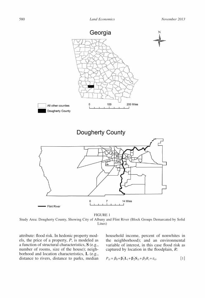
In 1994, the Flint River overran its banksfrom the effects of Tropical Storm Alberto,causing a major flood in southwestern Geor-gia. Dougherty County, where 15 people werekilled and almost 78,000 people were dis-placed by the flood, suffered the greatest dam-age. Divided by the Flint River into twohalves, Dougherty County was founded in theearly 1800s and today it is the core of a met-ropolitan area. Illustrated in Figure 1, it has atotal area of 334.64 square miles, of which329.60 square miles is land and 5.04 squaremiles is water (U.S. Census Bureau 2010).The city of Albany was hit worst by the flood.Peak discharges greater than the 100-yearflood discharge were recorded at all U.S. Geo-logical Survey (USGS) gauging stations onthe Flint River (Stamey 1996). According tothe USGS, the Flint River peaked at a stageabout five feet higher than that of a flood in1925, which was the previous maximum floodever recorded at Albany. The flood submergedmost of South Albany, inundating 4,200 res-idences, with $99.4 million in damages toresidential, commercial, and other structures;62,502 tons of flood debris dumped in land-fills; 4,907 workers temporarily unemployed;and $80 million in home and small businessloans issued by the Small Business Adminis-tration (Formwalt 1996).

According to the Federal Emergency Man-agement Agency (FEMA), nearly 20,000communities across the United States and itsterritories participate in the National Flood In-surance Program (NFIP). When a communityjoins the NFIP it agrees to adopt and enforcefloodplain management ordinances to reducefuture flood damage. In exchange, the NFIPmakes federally backed flood insurance avail-able to homeowners, renters, and businessowners in these communities. Federal floodinsurance was considered to be an economi-cally efficient way to indemnify flood victimsand to have individuals internalize some ofthe risk of property ownership in the flood-plains (Anderson 1974). Community partici-

pation in the NFIP is voluntary. In order toactuarially rate new construction for flood in-surance and create broad-based awareness ofthe flood hazards, FEMA maps 100-year and500-year floodplains in participating com-munities. These hazard zones are mutually ex-clusive, representing different annual proba-bilities of flooding: 1% and 0.2% in a givenyear, respectively. The city of Albany hasbeen a participating community in the NFIPsince 1974. All the other parts of DoughertyCounty joined the NFIP in 1978 (FEMA2012). Most homeowners with mortgages inthe 100-year floodplain are mandated to buyflood insurance, so they should be more awareof the associated flood hazard than homeown-ers of properties in the 500-year floodplain,who are not required to buy flood insurance.In our analysis we differentiate between thetwo types of properties.

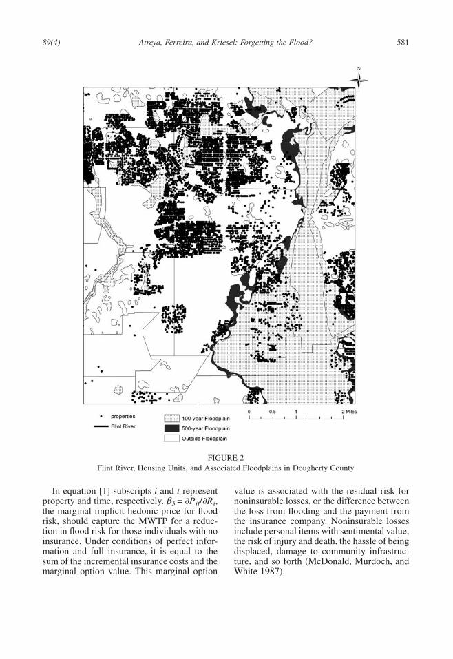
Figure 2 is a map of the Flint River, hous-ing units, and the associated floodplains forthe southwestern part of Dougherty County.Almost 10.7% of the properties sold betweenthe years of 1985 to 2004 fall in the flood-plain. Many properties in the designated floodhazard zones had not experienced a flood indecades. At the same time there have beencases of properties outside the 100-year floodzone that have unexpectedly experiencedfloods. In some cases, individuals in the 100-year flood plain may erroneously think thatsince they have experienced a flood, there willnot be more flooding for 100 years. In thesecases the risks and costs associated with livingin a flood-prone area may not be fully under-stood by homebuyers.

III. METHODS

Hedonic models (Rosen 1974; Freeman2003) have been used extensively to estimatethe contribution to the total value of a propertyof each characteristic possessed by the prop-erty. Hedonic property models have also beenproven to be an effective tool for estimatingthe marginal willingness to pay (MWTP) forchanges in environmental quality since theirearly applications in the late 1960s (Halstead,Bouvier, and Hansen 1997). Like earlier stud-ies we use a hedonic model to determine theshadow value of a nonmarket environmental


FIGURE 1Study Area: Dougherty County, Showing City of Albany and Flint River (Block Groups Demarcated by Solid

Lines)

attribute: flood risk. In hedonic property mod-els, the price of a property, P, is modeled asa function of structural characteristics, S (e.g.,number of rooms, size of the house); neigh-borhood and location characteristics, L (e.g.,distance to rivers, distance to parks, median

household income, percent of nonwhites inthe neighborhood); and an environmentalvariable of interest, in this case flood risk ascaptured by location in the floodplain, R:

′ ′P = β +β L +β S +β R + ε . [1]it 0 1 i 2 it 3 i it


FIGURE 2Flint River, Housing Units, and Associated Floodplains in Dougherty County

In equation [1] subscripts i and t representproperty and time, respectively. β3 it i,= ∂P /∂Rthe marginal implicit hedonic price for floodrisk, should capture the MWTP for a reduc-tion in flood risk for those individuals with noinsurance. Under conditions of perfect infor-mation and full insurance, it is equal to thesum of the incremental insurance costs and themarginal option value. This marginal option

value is associated with the residual risk fornoninsurable losses, or the difference betweenthe loss from flooding and the payment fromthe insurance company. Noninsurable lossesinclude personal items with sentimental value,the risk of injury and death, the hassle of beingdisplaced, damage to community infrastruc-ture, and so forth (McDonald, Murdoch, andWhite 1987).


Regarding the functional form, we per-formed a Box-Cox transformation of the de-pendent variable, and after comparing the re-sidual sum of squares we concluded that thenatural log of price as the dependent variablewas the best specification for our model. Aftertesting several transformations of the indepen-dent variables, the location variables L werebest fitted in their log form, while the otherattributes S were fitted best in their quadraticspecification, which is consistent with thefunctional form used by Bin and Polasky.

To measure flood risk we use two dummyvariables, one for the 100-year floodplain andone for the 500-year floodplain. There werearound 800 properties in zone D, whichFEMA defines as “an area of undeterminedbut possible flood hazard.” These propertieswere dropped from the analysis, but includingthem in the 100-year floodplain, or, alterna-tively, in the 500-year floodplain, did not af-fect the results.2 Thus, the hedonic modelwould be

′ ′ ′ 2ln(P ) = β +β ln L +β S +β Sit 0 1 i 2 it 3 it

+β 100yrFP +β 500yrFP +δ + ε . [2]4 i 5 i t it

The variable 100yrFP (100-year floodplain)in this model is a dummy equal to 1 if theproperty falls within the 100-year floodplainand 0 otherwise. Similarly, the variable500yrFP (500-year floodplain) is a dummyequal to 1 if the property falls within the 500-year floodplain and 0 otherwise. Year fixedeffects (δt) were included to capture annualshocks that may affect all of the properties.Throughout, we use heteroskedasticity-con-sistent standard errors.

In order to determine the effect of the 1994flood on property prices the DD model tradi-tionally used is

′ ′ ′ 2ln(P ) = β +β lnL +β S +β Sit 0 1 i 2 it 3 it

+β 100yrFP +β 500yrFP4 i 5 i

+β Flood +β 100yrFP *Flood6 it 7 i it

+β 500yrFP *Flood +δ + ε . [3]8 i it t it

2 These results are available upon request.

This DD model has been used in previousstudies (Bin and Landry, and Kousky) to ex-amine the information effects of a natural di-saster. In this model, properties that fall withina floodplain are the treatment group and prop-erties outside the floodplain are the controlgroup. The DD design allows us to isolate theeffect attributable to the flood from other con-temporaneous variables (e.g., macroeconomicchanges in the housing market, changes in thelocal housing market), since the control groupexperiences some or all of the contempora-neous influences that affect property values inthe treatment group but offers lower floodrisk. The variable Flood is a dummy variableequal to 1 if the sale happened after the flood(July 1994 in our case). The coefficient on theinteraction term between the 100-year flood-plain and the flood variables (100yrFP*Flood)tells us how the 1994 flood might have affectedthe prices of properties that are in the 100-yearfloodplain and that are sold after the 1994flood. A similar interpretation applies to the500-year floodplain and the flood dummy in-teraction.

An important econometric issue in hedonicmodels concerns the potential spatial depen-dence of the observations. Neighboring prop-erties are likely to share common unobservedlocation features, similar structural character-istics due to contemporaneous construction,neighborhood effects, and other causes of spa-tial dependence. Ignoring the problem couldresult in inefficient or inconsistent parameterestimates (Anselin and Bera 1998). Testingfor the presence of spatial dependence canproceed via maximum likelihood estimationof alternative models and applying appropri-ate Lagrange multiplier tests. Another ap-proach tests the significance of Moran’s I spa-tial autocorrelation coefficient estimated fromthe ordinary least squares (OLS) residuals.However, both approaches require the speci-fication of a spatial weights matrix.

As noted by Donovan, Champ, and Butry(2007), the specification of the matrix can bearbitrary and it can influence the outcome ofthe tests. To minimize the guess work, ouranalysis follows their lead and employs a se-mivariance analysis of the properties. This isa geostatistical technique that was first em-ployed in mining exploration but has since


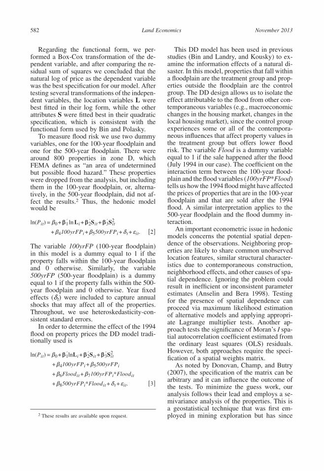
FIGURE 3Semivariance Graph of Observed (log) Prices and Ordinary Least Squares (OLS) Residuals

been used in varied fields including environ-mental health and hydrology (Cressie 1993).Following Cressie, the semivariance for pairsof parcels is given by

n(h)12γ (h) = (z(x + h)− z(x )) , [4]� i i

i = 12n(h)

where the z values are the parcels’ character-istic of interest, xi refers to the parcels, h is agiven distance interval between pairs of par-cels (we used 20 m), and n(h) is the numberof parcel pairs within the interval. Spatial de-pendence is indicated by increasing semivar-iance as the distance between pairs is in-creased, in other words, as properties losetheir grouping into neighborhoods they be-come less alike. If the semivariance is plottedover distance, insight into the weights matrixspecification can be obtained.

Figure 3 displays plots of two semivari-ances for pairs of properties within 20 m in-tervals, going out to 1,000 m.3 In the lowestplotted line, the regression’s residual semi-variance increases dramatically in the first in-

3 The analysis was conducted within SAS’s Proc Var-iogram.

tervals up to about 50 m, then it increasesslightly to 200 m, after which it levels off.Within the GIS overlay of Doughtery County,these distances are measured from the parcels’centroids rather than the actual houses. Giventhe size of the parcels, pairs within 50 m ofeach other tend to represent contiguous prop-erties. Pairs within 200 m of each other areseparated by four to six neighboring houses.The second plot of the semivariance of theregression’s dependent variable, the logarithmof property price, also increases dramaticallyfrom the origin, but it continues to increaseover the full range of distance intervals. Whilethe prices display the classic symptoms ofspatial dependence, the residuals display onlya neighbor effect. This comparison of the twoplots suggests that the regression model is ac-counting for the majority of spatial depen-dence with its set of spatial and neighbor-hood-level variables.

Concerning the spatial weights matrix, W,this analysis suggests that two different spec-ifications may be appropriate. In our estima-tion, we use two common parameterizationsfor W: a contiguity matrix, where adjacentproperties get a weight of one and zero oth-erwise, and an inverse distance matrix, whose


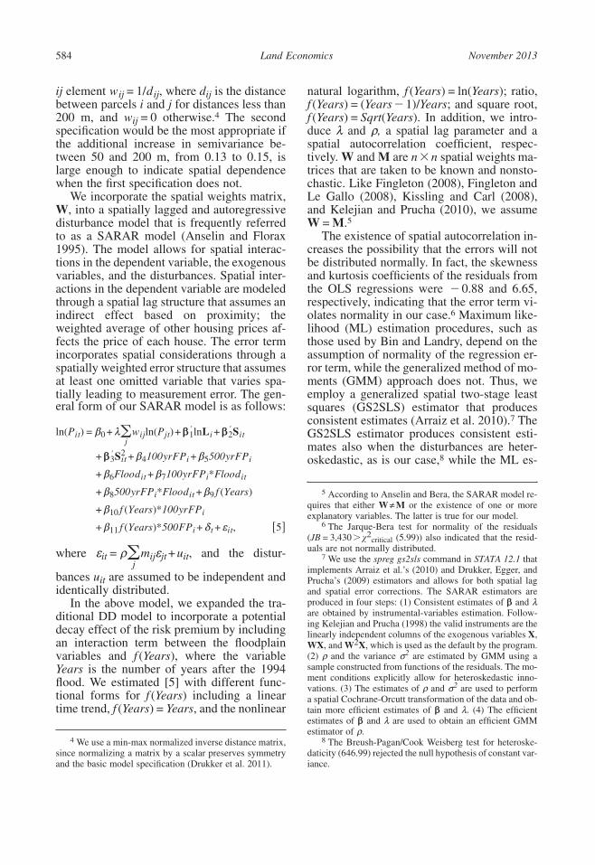
ij element ij ij, where dij is the distancew = 1/dbetween parcels i and j for distances less than200 m, and wij = 0 otherwise.4 The secondspecification would be the most appropriate ifthe additional increase in semivariance be-tween 50 and 200 m, from 0.13 to 0.15, islarge enough to indicate spatial dependencewhen the first specification does not.

We incorporate the spatial weights matrix,W, into a spatially lagged and autoregressivedisturbance model that is frequently referredto as a SARAR model (Anselin and Florax1995). The model allows for spatial interac-tions in the dependent variable, the exogenousvariables, and the disturbances. Spatial inter-actions in the dependent variable are modeledthrough a spatial lag structure that assumes anindirect effect based on proximity; theweighted average of other housing prices af-fects the price of each house. The error termincorporates spatial considerations through aspatially weighted error structure that assumesat least one omitted variable that varies spa-tially leading to measurement error. The gen-eral form of our SARAR model is as follows:

′ ′ln(P ) = β +λ w ln(P )+β lnL +β Sit 0 � ij jt 1 i 2 itj

′ 2+β S +β 100yrFP +β 500yrFP3 it 4 i 5 i

+β Flood +β 100yrFP *Flood6 it 7 i it

+β 500yrFP *Flood +β f (Years)8 i it 9

+β f (Years)*100yrFP10 i

+β f (Years)*500FP +δ + ε , [5]11 i t it

where εit = mijεjt +uit, and the distur-ρ�j

bances uit are assumed to be independent andidentically distributed.

In the above model, we expanded the tra-ditional DD model to incorporate a potentialdecay effect of the risk premium by includingan interaction term between the floodplainvariables and f (Years), where the variableYears is the number of years after the 1994flood. We estimated [5] with different func-tional forms for f (Years) including a lineartime trend, f (Years) = Years, and the nonlinear

4 We use a min-max normalized inverse distance matrix,since normalizing a matrix by a scalar preserves symmetryand the basic model specification (Drukker et al. 2011).

natural logarithm, f (Years) = ln(Years); ratio,f (Years) = (Years−1)/Years; and square root,f (Years) = Sqrt(Years). In addition, we intro-duce λ and ρ, a spatial lag parameter and aspatial autocorrelation coefficient, respec-tively. W and M are n×n spatial weights ma-trices that are taken to be known and nonsto-chastic. Like Fingleton (2008), Fingleton andLe Gallo (2008), Kissling and Carl (2008),and Kelejian and Prucha (2010), we assumeW = M.5

The existence of spatial autocorrelation in-creases the possibility that the errors will notbe distributed normally. In fact, the skewnessand kurtosis coefficients of the residuals fromthe OLS regressions were −0.88 and 6.65,respectively, indicating that the error term vi-olates normality in our case.6 Maximum like-lihood (ML) estimation procedures, such asthose used by Bin and Landry, depend on theassumption of normality of the regression er-ror term, while the generalized method of mo-ments (GMM) approach does not. Thus, weemploy a generalized spatial two-stage leastsquares (GS2SLS) estimator that producesconsistent estimates (Arraiz et al. 2010).7 TheGS2SLS estimator produces consistent esti-mates also when the disturbances are heter-oskedastic, as is our case,8 while the ML es-

5 According to Anselin and Bera, the SARAR model re-quires that either W≠ M or the existence of one or moreexplanatory variables. The latter is true for our model.

6 The Jarque-Bera test for normality of the residuals(JB = 3,430>v2

critical (5.99)) also indicated that the resid-uals are not normally distributed.

7 We use the spreg gs2sls command in STATA 12.1 thatimplements Arraiz et al.’s (2010) and Drukker, Egger, andPrucha’s (2009) estimators and allows for both spatial lagand spatial error corrections. The SARAR estimators areproduced in four steps: (1) Consistent estimates of β and λare obtained by instrumental-variables estimation. Follow-ing Kelejian and Prucha (1998) the valid instruments are thelinearly independent columns of the exogenous variables X,WX, and W2X, which is used as the default by the program.(2) ρ and the variance σ2 are estimated by GMM using asample constructed from functions of the residuals. The mo-ment conditions explicitly allow for heteroskedastic inno-vations. (3) The estimates of ρ and σ2 are used to performa spatial Cochrane-Orcutt transformation of the data and ob-tain more efficient estimates of β and λ. (4) The efficientestimates of β and λ are used to obtain an efficient GMMestimator of ρ.

8 The Breush-Pagan/Cook Weisberg test for heteroske-daticity (646.99) rejected the null hypothesis of constant var-iance.


timator could produce inconsistent estimatesin the presence of heteroskedasticity (Arraizet al. 2010).

IV. DATA

Our dataset combines individual propertysales data for residential homes in DoughertyCounty from the Dougherty County’s tax as-sessor’s office for the years 1985 to 2004, witha parcel-level GIS database.

In order to use the spatial weight matricesto control for the lag and error dependence inour model, we limit our sample to the mostrecent sale, that is, there are no repeatedsales.9 The property records contain infor-mation on housing characteristics (number ofbedrooms, number of bathrooms, total squarefootage, total acres, size of the house, etc.),vector S in equations [1]–[5], as well as saledate and sale price. All the property sale priceswere adjusted to 2004 constant dollars usingthe housing price index for the Albany met-ropolitan area from the Office of FederalHousing Enterprise Oversight (OFHEO).10

Regarding the proximity and neighborhoodvariables L, GIS was utilized to measure thedistance from each property to important fea-tures that could influence property values suchas nearby major highways, railroads, andamenities such as parks and rivers. The neigh-borhood characteristics (median householdincome and percent of nonwhite residents)were determined at the block group level us-ing 2000 census data.11 To measure flood risk,

9 To create an inverse distance matrix the observationsmust have unique coordinates. For a contiguity matrix theonly requirement is that the shape file of the dataset be apolygon.

10 We use the OFHEO index over other housing priceindices such as the Case-Shiller index. While the OFHEOindex is available for 363 metropolitan statistical areas(MSAs) including Albany, Georgia, which is the focus ofour study, the Case-Shiller index covers only 20 majorMSAs, which include Atlanta but not our study area. Visualinspection of the OFHEO indices for Atlanta and Albanysuggests that these are very different real estate markets sub-ject to different demand conditions. The growth rate of Cen-sus population figures for the Atlanta MSA was 3.1% peryear between 1985 and 2010, but only 0.56% for the AlbanyMSA.

11 Block groups generally contain between 600 and3,000 people, with a typical size of 1,500 people.

we used a GIS layer of FEMA Q3 flood datato identify parcels in 100-year and 500-yearfloodplains as represented on flood insurancerate maps published in 1996.12

Studies have shown that there are price pre-miums associated with elevated properties(McKenzie and Levendis 2010). To see if thatis true for Dougherty County, elevation ofeach property was determined using the GISfile of contour lines, by overlaying the prop-erties onto 1:100,000-scale elevation layersfor Dougherty County, which is produced byUSGS. There could be some houses that wereelevated more, especially after the commu-nity’s admission into the NFIP, to meet theminimum elevation requirements set by theprogram.13 In order to capture the additionalelevation effect, we control for the propertiesthat were built after 1978, that is, after theNFIP began. We included NFIP as a dummyequal to 1 if the property was built after 1978(0 otherwise).

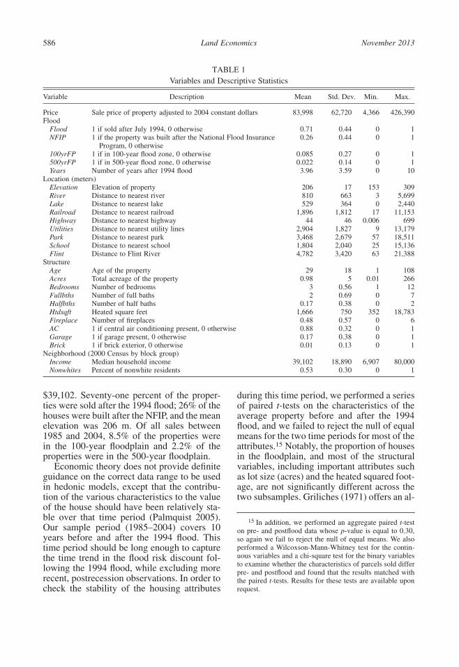
After dropping properties for which datawere missing, or whose sale price was lessthan $4,000 or more than $500,000, or thatwere not single-family residential properties,8,042 property transactions were included inthe dataset.14 Table 1 presents their descrip-tive statistics. The average house was 29 yearsold, with the oldest home built in 1885 andthe newest built in 2004. The mean propertyvalue in 2004 constant dollars was $83,998.The mean distance to the Flint River wasabout 4.8 km. The average of median house-hold incomes in the census block groups was

12 As part of a countywide flood map modernization pro-gram, the state of Georgia in cooperation with FEMA pub-lished a new floodplain map for Dougherty County in 2009.In our analysis, we choose the 1996 map, as the large floodevent in our study occurred in 1994 and all of our salestransaction occurred before 2009. In addition, the 1996 mapis the first digitized map that incorporates all of DoughertyCounty. Older, nondigitized maps are either for the city ofAlbany or for the rest of Dougherty County and not for thesame year.

13 Communities participating in the NFIP must fullycomply with its building code, which requires the lowestfloor of any new residential building to be elevated abovethe base flood elevation.

14 Properties sold for less than $4,000 were probablyfamily transfers and not real sales. Since the maximum NFIPcoverage is $250,000, flood insurance is less important forvery expensive houses.


TABLE 1Variables and Descriptive Statistics

Variable Description Mean Std. Dev. Min. Max.

Price Sale price of property adjusted to 2004 constant dollars 83,998 62,720 4,366 426,390Flood

Flood 1 if sold after July 1994, 0 otherwise 0.71 0.44 0 1NFIP 1 if the property was built after the National Flood Insurance

Program, 0 otherwise0.26 0.44 0 1

100yrFP 1 if in 100-year flood zone, 0 otherwise 0.085 0.27 0 1500yrFP 1 if in 500-year flood zone, 0 otherwise 0.022 0.14 0 1Years Number of years after 1994 flood 3.96 3.59 0 10

Location (meters)Elevation Elevation of property 206 17 153 309River Distance to nearest river 810 663 3 5,699Lake Distance to nearest lake 529 364 0 2,440Railroad Distance to nearest railroad 1,896 1,812 17 11,153Highway Distance to nearest highway 44 46 0.006 699Utilities Distance to nearest utility lines 2,904 1,827 9 13,179Park Distance to nearest park 3,468 2,679 57 18,511School Distance to nearest school 1,804 2,040 25 15,136Flint Distance to Flint River 4,782 3,420 63 21,388

StructureAge Age of the property 29 18 1 108Acres Total acreage of the property 0.98 5 0.01 266Bedrooms Number of bedrooms 3 0.56 1 12Fullbths Number of full baths 2 0.69 0 7Halfbths Number of half baths 0.17 0.38 0 2Htdsqft Heated square feet 1,666 750 352 18,783Fireplace Number of fireplaces 0.48 0.57 0 6AC 1 if central air conditioning present, 0 otherwise 0.88 0.32 0 1Garage 1 if garage present, 0 otherwise 0.17 0.38 0 1Brick 1 if brick exterior, 0 otherwise 0.01 0.13 0 1

Neighborhood (2000 Census by block group)Income Median household income 39,102 18,890 6,907 80,000Nonwhites Percent of nonwhite residents 0.53 0.30 0 1

$39,102. Seventy-one percent of the proper-ties were sold after the 1994 flood; 26% of thehouses were built after the NFIP, and the meanelevation was 206 m. Of all sales between1985 and 2004, 8.5% of the properties werein the 100-year floodplain and 2.2% of theproperties were in the 500-year floodplain.

Economic theory does not provide definiteguidance on the correct data range to be usedin hedonic models, except that the contribu-tion of the various characteristics to the valueof the house should have been relatively sta-ble over that time period (Palmquist 2005).Our sample period (1985–2004) covers 10years before and after the 1994 flood. Thistime period should be long enough to capturethe time trend in the flood risk discount fol-lowing the 1994 flood, while excluding morerecent, postrecession observations. In order tocheck the stability of the housing attributes

during this time period, we performed a seriesof paired t-tests on the characteristics of theaverage property before and after the 1994flood, and we failed to reject the null of equalmeans for the two time periods for most of theattributes.15 Notably, the proportion of housesin the floodplain, and most of the structuralvariables, including important attributes suchas lot size (acres) and the heated squared foot-age, are not significantly different across thetwo subsamples. Griliches (1971) offers an al-

15 In addition, we performed an aggregate paired t-teston pre- and postflood data whose p-value is equal to 0.30,so again we fail to reject the null of equal means. We alsoperformed a Wilcoxson-Mann-Whitney test for the contin-uous variables and a chi-square test for the binary variablesto examine whether the characteristics of parcels sold differpre- and postflood and found that the results matched withthe paired t-tests. Results for these tests are available uponrequest.


ternative guide to aggregation over time in he-donic regressions, based on the comparison ofthe standard errors in the constrained and un-constrained regressions. Aggregation is re-jected if the standard error increases by morethan 10%. We compared the standard error ofthe regression using the 1985–2004 samplewith that of regressions using subsets of thedata that utilize shorter time periods (1989–1999, 1985–1994, 1994–2004) and found thatthe increase in standard error was not largerthan 1% in any case, and thus we decided onthe 1985–2004 sample to capture the decay inthe flood risk discount over the longer timeperiod.

V. RESULTS

Estimates of the SARAR Model Using aContiguity Matrix

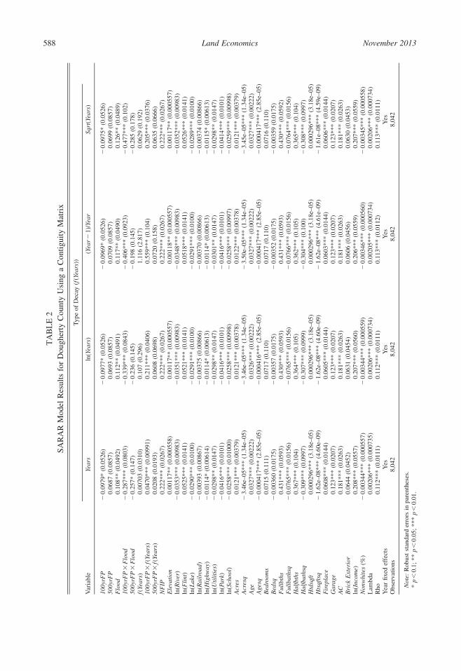
Table 2 shows the coefficient estimates ofequation [5], the SARAR model, using a con-tiguity matrix as the spatial weights matrix.The columns differ in terms of the functionalform of the time-decay effect, f (Years).

The significant spatial autocorrelation pa-rameter (ρ) and spatial autoregressive coeffi-cient (λ), toward the bottom of Table 2, sug-gest that for all the specifications there is, infact, spatial dependence among the propertiesin our dataset in the expected direction: a posi-tive adjacency effect. We expect a positive λsince, for example, a higher sale price ofneighboring properties should result in ahigher average sale price, ceteris paribus.Conforming to intuition, λ is significant at a1% level and robustly estimated at 0.002across the specifications, indicating that if theweighted average of neighboring houses’ saleprice increases by 1%, the sale price of anindividual house increases by approximately0.002%. Regarding the interpretation of theregression coefficients, in the spatial lagmodel, marginal effects are calculated by mul-tiplying the estimates times a spatial multi-plier, 1/(1−λ) (Kim, Phipps, and Anselin2003). A larger λ means a larger spatial de-pendence and, thus, a larger spatial multiplier.

The coefficient for NFIP is positive and sig-nificant, implying that homes constructed un-der the more stringent building codes, and for

which, ceteris paribus, expected flood dam-ages should be lower, are worth more. Theneighborhood variables, median household in-come and percent of nonwhite residents byblock group, have an expected significant posi-tive and negative sign, respectively. All coef-ficients for the structural housing characteris-tics have the expected sign and most of themare statistically significant. The quadratic spec-ification seems to capture diminishing mar-ginal effects for acres, age, full baths, halfbaths, and heated squared footage. The resultsindicate that proximity to rivers (except for theFlint River), lakes and ponds, highways, utilitylines, parks, and schools increases the propertyprices significantly. There was a small pricepremium associated with elevated properties;when evaluated for an average priced home,the premium per meter equals almost $98across all the decay functions.

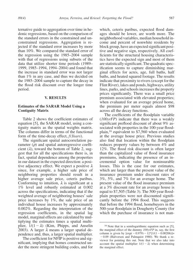
The coefficients of the floodplain variable(100yrFP) indicate that there was a weaklysignificant preflood discount of about 9% as-sociated with properties in the 100-year flood-plain,16 equivalent to $7,560 when evaluatedat the average house price. Previous studiesalso find that location within the floodplainreduces property values by between 4% and12%. The flood risk discount is often largerthan the capitalized value of flood insurancepremiums, indicating the presence of an in-cremental option value for noninsurablelosses. This is the case for our estimates,which are larger than the present value of theinsurance premium under discount rates of3%, 5%, and 7% for an average home. Thepresent value of the flood insurance premiumat a 3% discount rate for an average house isequal to $7,505 (Table 3). The 500-year flood-plain properties were not discounted signifi-cantly before the 1994 flood. This suggeststhat before the 1994 flood, homebuyers in the500-year floodplain in Dougherty County (forwhich the purchase of insurance is not man-

16 Note that in a semilogarithmic equation such as [5],the marginal effect of the dummy 100yrFP in, say, the firstcolumn is given by [exp(−0.979)−1]*[1/(1−0.00206)]=−0.09 (Halvorsen and Palmquist 1980). We thank a re-viewer for pointing this out. Note that we also take intoaccount the spatial multiplier 1/(1−λ) when determiningthe marginal effect.

November 2013Land Economics588T

AB

LE

2SA

RA

RM

odel

Res

ults

for

Dou

gher

tyC

ount

yU

sing

aC

ontig

uity

Mat

rix

Type

ofD

ecay

(f(Y

ears

))

Var

iabl

eYe

ars

ln(Y

ears

)(Y

ear−

1)/Y

ear

Sqrt

(Yea

rs)

100y

rFP

−0.

0979

*(0

.052

6)−

0.09

77*

(0.0

526)

−0.

0969

*(0

.052

6)−

0.09

75*

(0.0

526)

500y

rFP

0.06

87(0

.085

7)0.

0693

(0.0

857)

0.07

09(0

.085

7)0.

0699

(0.0

857)

Flo

od0.

108*

*(0

.049

2)0.

112*

*(0

.049

1)0.

117*

*(0

.049

0)0.

126*

*(0

.048

9)10

0yrF

P×

Flo

od−

0.28

7***

(0.0

803)

−0.

339*

**(0

.084

3)−

0.40

6***

(0.0

923)

−0.

477*

**(0

.102

)50

0yrF

P×

Flo

od−

0.25

7*(0

.147

)−

0.23

6(0

.145

)−

0.19

8(0

.145

)−

0.28

5(0

.178

)f(

Year

s)0.

0070

3(0

.031

0)0.

107

(0.2

96)

1.11

6(2

.817

)0.

0629

(0.1

92)

100y

rFP

×f(

Year

s)0.

0470

***

(0.0

0991

)0.

211*

**(0

.040

6)0.

559*

**(0

.104

)0.

205*

**(0

.037

6)50

0yrF

P×

f(Ye

ars)

0.02

08(0

.019

3)0.

0608

(0.0

698)

0.07

20(0

.158

)0.

0635

(0.0

666)

NF

IP0.

222*

**(0

.026

7)0.

222*

**(0

.026

7)0.

222*

**(0

.026

7)0.

222*

**(0

.026

7)E

leva

tion

0.00

117*

*(0

.000

558)

0.00

117*

*(0

.000

557)

0.00

118*

*(0

.000

557)

0.00

117*

*(0

.000

557)

ln(R

iver

)−

0.03

53**

*(0

.009

83)

−0.

0351

***

(0.0

0983

)−

0.03

48**

*(0

.009

83)

−0.

0352

***

(0.0

0983

)ln

(Fli

nt)

0.05

25**

*(0

.014

1)0.

0521

***

(0.0

141)

0.05

18**

*(0

.014

1)0.

0526

***

(0.0

141)

ln(L

ake)

−0.

0290

***

(0.0

100)

−0.

0291

***

(0.0

100)

−0.

0291

***

(0.0

100)

−0.

0289

***

(0.0

100)

ln(R

ailr

oad)

−0.

0039

3(0

.008

67)

−0.

0037

5(0

.008

66)

−0.

0037

0(0

.008

66)

−0.

0037

4(0

.008

66)

ln(H

ighw

ay)

−0.

0114

*(0

.006

14)

−0.

0114

*(0

.006

13)

−0.

0114

*(0

.006

13)

−0.

0115

*(0

.006

13)

ln(U

tili

ties

)−

0.02

98**

(0.0

147)

−0.

0298

**(0

.014

7)−

0.03

01**

(0.0

147)

−0.

0298

**(0

.014

7)ln

(Par

k)−

0.04

16**

*(0

.010

1)−

0.04

16**

*(0

.010

1)−

0.04

16**

*(0

.010

1)−

0.04

14**

*(0

.010

1)ln

(Sch

ool)

−0.

0258

***

(0.0

1000

)−

0.02

58**

*(0

.009

98)

−0.

0258

***

(0.0

0997

)−

0.02

59**

*(0

.009

98)

Acr

es0.

0121

***

(0.0

0379

)0.

0121

***

(0.0

0378

)0.

0122

***

(0.0

0378

)0.

0121

***

(0.0

0379

)A

cres

q−

3.46

e–05

***

(1.3

4e–0

5)−

3.46

e–05

***

(1.3

4e–0

5)−

3.50

e–05

***

(1.3

4e–0

5)−

3.45

e–05

***

(1.3

4e–0

5)A

ge0.

0327

***

(0.0

0222

)0.

0326

***

(0.0

0222

)0.

0327

***

(0.0

0222

)0.

0327

***

(0.0

0222

)A

gesq

−0.

0004

17**

*(2

.85e

–05)

−0.

0004

16**

*(2

.85e

–05)

−0.

0004

17**

*(2

.85e

–05)

−0.

0004

17**

*(2

.85e

–05)

Bed

room

s0.

0715

(0.1

11)

0.07

17(0

.110

)0.

0717

(0.1

10)

0.07

16(0

.110

)B

edsq

−0.

0036

0(0

.017

5)−

0.00

357

(0.0

175)

−0.

0035

2(0

.017

5)−

0.00

359

(0.0

175)

Ful

lbth

s0.

431*

**(0

.059

3)0.

430*

**(0

.059

3)0.

431*

**(0

.059

3)0.

430*

**(0

.059

2)F

ullb

aths

q−

0.07

65**

*(0

.015

6)−

0.07

65**

*(0

.015

6)−

0.07

66**

*(0

.015

6)−

0.07

64**

*(0

.015

6)H

alfb

ths

0.36

7***

(0.1

04)

0.36

4***

(0.1

05)

0.36

2***

(0.1

05)

0.36

5***

(0.1

04)

Hal

fbat

hsq

−0.

309*

**(0

.099

7)−

0.30

7***

(0.0

999)

−0.

304*

**(0

.100

)−

0.30

8***

(0.0

997)

Htd

sqft

0.00

0296

***

(3.1

8e–0

5)0.

0002

96**

*(3

.18e

–05)

0.00

0296

***

(3.1

8e–0

5)0.

0002

96**

*(3

.18e

–05)

Hts

qfts

q−

1.62

e–08

***

(4.6

0e–0

9)−

1.62

e–08

***

(4.6

0e–0

9)−

1.62

e–08

***

(4.6

1e–0

9)−

1.61

e–08

***

(4.5

9e–0

9)F

irep

lace

0.06

08**

*(0

.014

4)0.

0605

***

(0.0

144)

0.06

03**

*(0

.014

4)0.

0606

***

(0.0

144)

Gar

age

0.12

3***

(0.0

207)

0.12

3***

(0.0

207)

0.12

3***

(0.0

207)

0.12

3***

(0.0

207)

AC

0.18

1***

(0.0

263)

0.18

1***

(0.0

263)

0.18

1***

(0.0

263)

0.18

1***

(0.0

263)

Bri

ckE

xter

ior

0.06

44(0

.045

2)0.

0631

(0.0

454)

0.06

06(0

.045

6)0.

0630

(0.0

453)

ln(I

ncom

e)0.

208*

**(0

.055

7)0.

207*

**(0

.056

0)0.

206*

**(0

.055

9)0.

207*

**(0

.055

9)N

onw

hite

s(%

)−

0.00

344*

**(0

.000

557)

−0.

0034

4***

(0.0

0055

9)−

0.00

346*

**(0

.000

560)

−0.

0034

5***

(0.0

0055

8)L

ambd

a0.

0020

6***

(0.0

0073

5)0.

0020

6***

(0.0

0073

4)0.

0020

5***

(0.0

0073

4)0.

0020

6***

(0.0

0073

4)R

ho0.

112*

**(0

.011

1)0.

112*

**(0

.011

1)0.

113*

**(0

.011

2)0.

113*

**(0

.011

1)Y

ear

fixed

effe

cts

Yes

Yes

Yes

Yes

Obs

erva

tions

8,04

28,

042

8,04

28,

042

Not

e:R

obus

tst

anda

rder

rors

inpa

rent

hese

s.*

p<

0.1;

**p

<0.

05;*

**p

<0.

01.


TABLE 3Present Value of Flood Insurance Premiums at Various Discount Rates

Present Value of Insurance Premiumsunder Discount Rates of

Value of HousesAnnual Flood Insurance

Premium 3% 5% 7%

$75,000 $203 $6,742 $4,055 $2,896$83,998 $226 $7,505 $4,514 $3,224$200,000 $540 $17,999 $10,800 $7,714

Note: The flood insurance premium for an average-valued single-family house in the 100-year floodplain,without a basement and with estimated base flood elevation of 3 ft or more, is equal to $226. This is calculatedusing 0.27 as the annual postfirm construction rate per $100 of coverage as designated in the National FloodInsurance Program flood insurance manual.

datory) were probably unaware of the floodrisk, and, therefore, the flood risk was not cap-italized into property prices.

In a DD framework, assuming that prop-erties outside the floodplain represent a validcontrol group, the causal effect of the 1994major flood event on flood prone property val-ues is reflected in the coefficients of the inter-action terms between the flood and floodplaindummies. The results in the first column ofTable 2 indicate that immediately after the1994 flood, with the linear time decay func-tion, there is a 32% discount for the 100-yearfloodplain properties. This includes a 9%baseline flood zone estimate, calculated fromthe coefficient for the 100yrFP variable, plus23% calculated from the 100yrFP*Floodcoefficient.17 This discount is equivalent to$26,880 evaluated for an average-pricedhome in Dougherty County. With the nonlin-ear decay functions the initial increase in riskdiscount immediately following the flood iseven higher, with the price differential be-tween 35% and 44%. This is consistent withthe results of Bin and Landry, namely, the dis-counts with nonlinear time decay functionsare higher than with the linear time trend. Thediscount for 500-year floodplain propertieswas almost 23% with a linear decay function,although weakly significant and not robustacross different decay specifications.

The large price drop for the 100-year floodzone properties induced by the flood, how-ever, is not persistent over time. The flood risk

17 The discount is calculated following Halvorsen andPalmquist as [exp(−0.0979−0.287)−1]*[1/(1−0.00206)]=0.320.

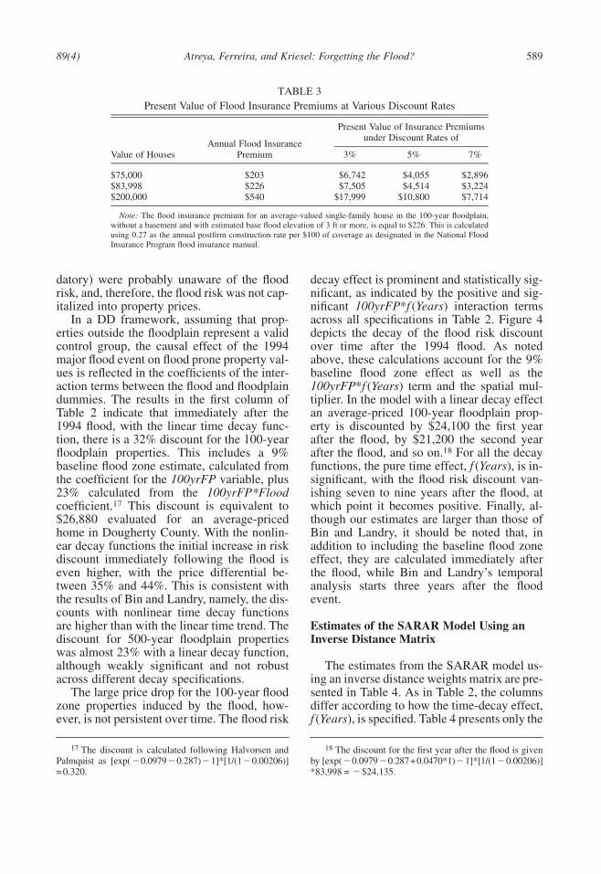
decay effect is prominent and statistically sig-nificant, as indicated by the positive and sig-nificant 100yrFP*f (Years) interaction termsacross all specifications in Table 2. Figure 4depicts the decay of the flood risk discountover time after the 1994 flood. As notedabove, these calculations account for the 9%baseline flood zone effect as well as the100yrFP*f (Years) term and the spatial mul-tiplier. In the model with a linear decay effectan average-priced 100-year floodplain prop-erty is discounted by $24,100 the first yearafter the flood, by $21,200 the second yearafter the flood, and so on.18 For all the decayfunctions, the pure time effect, f (Years), is in-significant, with the flood risk discount van-ishing seven to nine years after the flood, atwhich point it becomes positive. Finally, al-though our estimates are larger than those ofBin and Landry, it should be noted that, inaddition to including the baseline flood zoneeffect, they are calculated immediately afterthe flood, while Bin and Landry’s temporalanalysis starts three years after the floodevent.

Estimates of the SARAR Model Using anInverse Distance Matrix

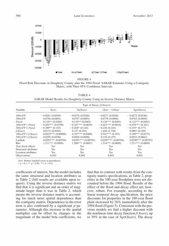
The estimates from the SARAR model us-ing an inverse distance weights matrix are pre-sented in Table 4. As in Table 2, the columnsdiffer according to how the time-decay effect,f (Years), is specified. Table 4 presents only the

18 The discount for the first year after the flood is givenby [exp(−0.0979−0.287+0.0470*1)−1]*[1/(1−0.00206)]*83,998 = −$24,135.


FIGURE 4Flood Risk Discounts in Dougherty County after the 1994 Flood: SARAR Estimates Using a Contiguity

Matrix, with Their 95% Confidence Intervals

TABLE 4SARAR Model Results for Dougherty County Using an Inverse Distance Matrix

Type of Decay (f (Years))

Variable Years ln(Years) (Year−1)/Year Sqrt(Years)

100yrFP −0.0261 (0.0549) −0.0276 (0.0548) −0.0271 (0.0548) −0.0272 (0.0548)500yrFP 0.0756 (0.0894) 0.0757 (0.0895) 0.0776 (0.0896) 0.0763 (0.0894)Flood 0.116** (0.0484) 0.119** (0.0483) 0.124*** (0.0481) 0.132*** (0.0481)100yrFP×Flood −0.292*** (0.0798) −0.347*** (0.0839) −0.423*** (0.0916) −0.470*** (0.101)500yrFP×Flood −0.289** (0.145) −0.268* (0.144) −0.230 (0.144) −0.335* (0.177)f (Years) 0.0133 (0.0305) 0.157 (0.291) 1.428 (2.758) 0.0967 (0.189)100yrFP× f (Years) 0.0425*** (0.00988) 0.197*** (0.0406) 0.541*** (0.103) 0.189*** (0.0375)500yrFP× f (Years) 0.0295 (0.0190) 0.0926 (0.0690) 0.138 (0.155) 0.0933 (0.0662)Lambda 0.0293*** (0.00794) 0.0291*** (0.00792) 0.0287*** (0.00794) 0.0290*** (0.00792)Rho 1.511*** (0.0899) 1.509*** (0.0897) 1.514*** (0.0899) 1.511*** (0.0899)Year fixed effects Yes Yes Yes YesStructural attributes Yes Yes Yes YesLocation attributes Yes Yes Yes YesObservations 8,042 8,042 8,042 8,042

Note: Robust standard errors in parentheses.* p<0.1; ** p<0.05; *** p<0.01.

coefficients of interest, but the model includesthe same structural and location attributes asin Table 2 (full results are available upon re-quest). Using the inverse distance matrix wefind that λ is significant and an order of mag-nitude larger than it was in Table 2, whichmeans the inverse distance matrix is account-ing for much more spatial dependence thanthe contiguity matrix. Dependence in the errorterm is also confirmed by a significant pa-ρrameter. Although this increase in the spatialmultiplier can be offset by changes in themagnitude of the model beta coefficients, we

find that in contrast with results from the con-tiguity matrix specifications, in Table 2, prop-erties in the 100-year floodplain were not dis-counted before the 1994 flood. Results of theeffect of the flood and decay effect are, how-ever, robust. For example, according to thelinear temporal decay specification, the pricediscounts for properties in the 100-year floodplain increased by 26% immediately after the1994 flood (Figure 5). Consistent with the pre-vious models we find a higher discount withthe nonlinear time decay function f (Years), upto 39% in the case of Sqrt(Years). The decay


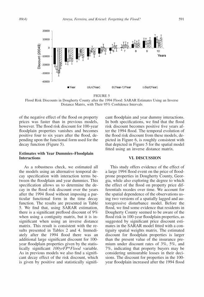
FIGURE 5Flood Risk Discounts in Dougherty County after the 1994 Flood: SARAR Estimates Using an Inverse

Distance Matrix, with Their 95% Confidence Intervals

of the negative effect of the flood on propertyprices was faster than in previous models,however. The flood risk discount for 100-yearfloodplain properties vanishes and becomespositive four to six years after the flood, de-pending upon the functional form used for thedecay function (Figure 5).

Estimates with Year Dummies–FloodplainInteractions

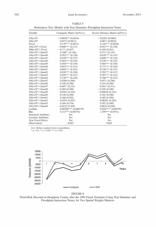
As a robustness check, we estimated allthe models using an alternative temporal de-cay specification with interaction terms be-tween the floodplain and year dummies. Thisspecification allows us to determine the de-cay in the flood risk discount over the yearsafter the 1994 flood without imposing a par-ticular functional form in the time decayfunction. The results are presented in Table5. We find that, using SARAR estimation,there is a significant preflood discount of 9%when using a contiguity matrix, but it is in-significant when using an inverse distancematrix. This result is consistent with the re-sults presented in Tables 2 and 4. Immedi-ately after the 1994 flood there was anadditional large significant discount for 100-year floodplain properties given by the statis-tically significant 100yrFP*Flood variable.As in previous models we also find a signifi-cant decay effect of the risk discount, whichis given by positive and statistically signifi-

cant floodplain and year dummy interactions.In both specifications, we find that the floodrisk discount becomes positive five years af-ter the 1994 flood. The temporal evolution ofthe flood risk discount from these models, de-picted in Figure 6, is roughly consistent withthat depicted in Figure 5 for the spatial modelfitted using an inverse distance matrix.

VI. DISCUSSION

This study offers evidence of the effect ofa large 1994 flood event on the price of flood-prone properties in Dougherty County, Geor-gia, while also exploring the degree to whichthe effect of the flood on property price dif-ferentials recedes over time. We account forthe spatial dependence of the observations us-ing two versions of a spatially lagged and au-toregressive disturbance model. Before theflood, we find some evidence that residents inDougherty County seemed to be aware of theflood risk in 100-year floodplain properties, assuggested by significant price discount esti-mates in the SARAR model fitted with a con-tiguity spatial weights matrix. The estimateddiscount for floodplain properties is largerthan the present value of the insurance pre-mium under discount rates of 3%, 5%, and7%, indicating that property buyers may beconsidering uninsurable losses in their deci-sions. The discount for properties in the 100-year floodplain increased after the 1994 flood


TABLE 5Robustness Test: Models with Year Dummies–Floodplain Interaction Terms

Variable Contiguity Matrix ln(Price) Inverse Distance Matrix ln(Price)

100yrFP −0.0936** (0.0454) −0.0202 (0.0483)500yrFP 0.0723 (0.0812) 0.0871 (0.0818)Flood 0.139*** (0.0531) 0.144*** (0.0520)100yrFP×Flood −0.660*** (0.131) −0.652*** (0.128)500yr FP×Flood −0.171 (0.267) −0.189 (0.261)100yrFP×Dum95 0.340** (0.146) 0.271* (0.143)100yrFP×Dum96 0.592*** (0.150) 0.639*** (0.147)100yrFP×Dum97 0.630*** (0.157) 0.608*** (0.154)100yrFP×Dum98 0.564*** (0.155) 0.536*** (0.152)100yrFP×Dum99 0.594*** (0.159) 0.584*** (0.156)100yrFP×Dum00 0.852*** (0.152) 0.771*** (0.149)100yrFP×Dum01 0.804*** (0.161) 0.736*** (0.157)100yrFP×Dum02 0.838*** (0.150) 0.782*** (0.147)100yrFP×Dum03 0.659*** (0.147) 0.591*** (0.143)100yrFP×Dum04 0.730*** (0.148) 0.706*** (0.145)500yrFP×Dum95 0.0280 (0.306) 0.0371 (0.298)500yrFP×Dum96 0.190 (0.298) 0.163 (0.290)500yrFP×Dum97 −0.607* (0.321) −0.561* (0.311)500yrFP×Dum98 −0.289 (0.308) −0.259 (0.300)500yrFP×Dum99 0.0101 (0.324) −0.00618 (0.316)500yrFP×Dum00 0.148 (0.298) 0.182 (0.290)500yrFP×Dum01 0.360 (0.302) 0.402 (0.296)500yrFP×Dum02 −0.0391 (0.287) 0.00281 (0.283)500yrFP×Dum03 0.368 (0.318) 0.392 (0.309)500yrFP×Dum04 −0.0232 (0.305) 0.0634 (0.298)Lambda 0.00200*** (0.000739) 0.0287*** (0.00795)Rho 0.113*** (0.00774) 1.559*** (0.0751)Structural Attributes Yes YesLocation Attributes Yes YesYear Fixed Effects Yes YesObservations 8,042 8,042

Note: Robust standard errors in parentheses.* p<0.1; ** p<0.05; *** p<0.01.

FIGURE 6Flood Risk Discount in Dougherty County after the 1994 Flood: Estimates Using Year Dummies and

Floodplain Interaction Terms, for Two Spatial Weights Matrices


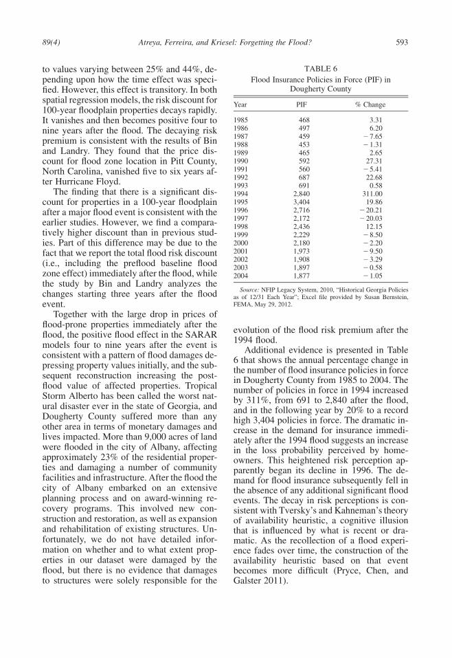
TABLE 6Flood Insurance Policies in Force (PIF) in

Dougherty County

Year PIF % Change

1985 468 3.311986 497 6.201987 459 −7.651988 453 −1.311989 465 2.651990 592 27.311991 560 −5.411992 687 22.681993 691 0.581994 2,840 311.001995 3,404 19.861996 2,716 −20.211997 2,172 −20.031998 2,436 12.151999 2,229 −8.502000 2,180 −2.202001 1,973 −9.502002 1,908 −3.292003 1,897 −0.582004 1,877 −1.05

Source: NFIP Legacy System, 2010, “Historical Georgia Policiesas of 12/31 Each Year”; Excel file provided by Susan Bernstein,FEMA, May 29, 2012.

to values varying between 25% and 44%, de-pending upon how the time effect was speci-fied. However, this effect is transitory. In bothspatial regression models, the risk discount for100-year floodplain properties decays rapidly.It vanishes and then becomes positive four tonine years after the flood. The decaying riskpremium is consistent with the results of Binand Landry. They found that the price dis-count for flood zone location in Pitt County,North Carolina, vanished five to six years af-ter Hurricane Floyd.

The finding that there is a significant dis-count for properties in a 100-year floodplainafter a major flood event is consistent with theearlier studies. However, we find a compara-tively higher discount than in previous stud-ies. Part of this difference may be due to thefact that we report the total flood risk discount(i.e., including the preflood baseline floodzone effect) immediately after the flood, whilethe study by Bin and Landry analyzes thechanges starting three years after the floodevent.

Together with the large drop in prices offlood-prone properties immediately after theflood, the positive flood effect in the SARARmodels four to nine years after the event isconsistent with a pattern of flood damages de-pressing property values initially, and the sub-sequent reconstruction increasing the post-flood value of affected properties. TropicalStorm Alberto has been called the worst nat-ural disaster ever in the state of Georgia, andDougherty County suffered more than anyother area in terms of monetary damages andlives impacted. More than 9,000 acres of landwere flooded in the city of Albany, affectingapproximately 23% of the residential proper-ties and damaging a number of communityfacilities and infrastructure. After the flood thecity of Albany embarked on an extensiveplanning process and on award-winning re-covery programs. This involved new con-struction and restoration, as well as expansionand rehabilitation of existing structures. Un-fortunately, we do not have detailed infor-mation on whether and to what extent prop-erties in our dataset were damaged by theflood, but there is no evidence that damagesto structures were solely responsible for the

evolution of the flood risk premium after the1994 flood.

Additional evidence is presented in Table6 that shows the annual percentage change inthe number of flood insurance policies in forcein Dougherty County from 1985 to 2004. Thenumber of policies in force in 1994 increasedby 311%, from 691 to 2,840 after the flood,and in the following year by 20% to a recordhigh 3,404 policies in force. The dramatic in-crease in the demand for insurance immedi-ately after the 1994 flood suggests an increasein the loss probability perceived by home-owners. This heightened risk perception ap-parently began its decline in 1996. The de-mand for flood insurance subsequently fell inthe absence of any additional significant floodevents. The decay in risk perceptions is con-sistent with Tversky’s and Kahneman’s theoryof availability heuristic, a cognitive illusionthat is influenced by what is recent or dra-matic. As the recollection of a flood experi-ence fades over time, the construction of theavailability heuristic based on that eventbecomes more difficult (Pryce, Chen, andGalster 2011).


Another potential driver of changes in theprice differential between houses inside andoutside the 100-year floodplain could bechanges in flood insurance premiums. How-ever, insurance rates are exogenous and didnot change after the 1994 flood.19 In fact, thenational average flood insurance premium perpolicy between 1994 and 1995 fell by about0.63% in real terms (FEMA 2013). The floodelevation of the first floor of the structure rela-tive to the flood depth on the floodplain de-termines property-specific flood risk data toguide construction and insurance decisions.Before FEMA began its map modernizationprograms in 2003, many flood insurance riskmaps on which the flood insurance rates arebased were 20 to 25 years old and did notaccurately reflect residual risk behind or be-low flood control structures, giving residentsliving behind them a false sense of security(King 2011). Moreover, even if the insurancerates had increased, Kriesel and Landry(2004) show that the purchase of NFIP poli-cies is inelastic with respect to price.

Acknowledgments

Financial support of the USGS/Georgia Water Re-sources Institute grant #2521RC282387 (Atreya andFerreira) is gratefully acknowledged. We thank SusanBernstein at FEMA for sharing with us the data inTable 6.

References

Anderson, Dan R. 1974. “The National Flood Insur-ance Program: Problem and Potential.” Journal ofRisk and Insurance 16 (4): 579–99.

Anselin, Luc, and Anil K. Bera. 1998. “Spatial De-pendence in Linear Regression Models with an In-troduction to Spatial Econometrics.” In Handbookof Applied Economic Statistics, Vol. 155, ed.Aman Ullah and David E. A. Giles, 237–90. NewYork: Marcel Dekker.

Anselin, Luc, and Raymond J. G. M. Florax. 1995.“Small Sample Properties of Tests for Spatial De-pendence in Regression Models: Some FurtherResults.” In New Directions in Spatial Economet-rics, ed. Luc Anselin and Raymond J. G. M.Florax, 21–74. Berlin: Springer-Verlag.

19 Susan Bernstein, FEMA, personal communication,September 2012.

Arraiz, Irani, David M. Drukker, Harry H. Kelejian,and Ingmar R. Prucha. 2010. “A Spatial Cliff-OrdType Model with Heteroskedastic Innovations:Small and Large Sample Results.” Journal of Re-gional Science 50 (2): 592–614.

Beatley, Timothy, David J. Brower, and Anna K.Schwab. 2002. An Introduction to Coastal ZoneManagement, 2nd ed. Washington, DC: IslandPress.

Bin, Okmyung, and Jamie B. Kruse. 2006. “Real Es-tate Market Response to Coastal Flood Hazards.”Natural Hazards Review 7 (4): 137–44.

Bin, Okmyung, Jamie B. Kruse, and Craig E. Landry.2008. “Flood Hazards, Insurance Rates, andAmenities: Evidence from the Coastal HousingMarket.” Journal of Risk and Insurance 75 (1):63–82.

Bin, Okmyung, and Craig E. Landry. 2012. “Changesin Implicit Flood Risk Premiums: Empirical Evi-dence from the Housing Market.” Journal of En-vironmental Economics and Management 65 (3):361–76.

Bin, Okmyung, and Stephen Polasky. 2004. “Effectsof Flood Hazards on Property Values: Evidencebefore and after Hurricane Floyd.” Land Econom-ics 80 (4): 490–500.

Burby, Raymond J. 2001. “Flood Insurance andFloodplain Management: The U.S. Experience.”Global Environmental Change Part B: Environ-mental Hazards 3 (3–4): 111–22.

Carbone, Jared C., Daniel G. Hallstrom, and V. KerrySmith. 2006. “Can Natural Experiments MeasureBehavioral Responses to Environmental Risks?”Environmental and Resource Economics 33 (3):273–97.

Center for Research of the Epidemiology of Disasters(CRED). 2010. EM-DAT: International DisasterDatabase. Brussels: Universite Catholique deLouvain. Available at www.emdat.be.

Cressie, Noel. 1993. Statistics for Spatial Data. NewYork: Wiley and Sons.

Donovan, Geoffrey H., Patricia A. Champ, and DavidT. Butry. 2007. “Wildfire Risk and Housing Prices:A Case Study from Colorado Springs.” Land Eco-nomics 83 (2): 217–33.

Drukker, David M., Peter Egger, and Ingmar R. Pru-cha. 2009. On Single Equation GMM Estimationof a Spatial Autoregressive Model with SpatiallyAutoregressive Disturbance. Technical report, De-partment of Economics, University of Maryland.

Drukker, David M., Hua Peng, Ingmar R. Prucha, andRafal Raciborski. 2011. Creating and ManagingSpatial Weighting Matrices Using the Spmat Com-mand. Available at http://econweb.umd.edu/�pru-cha/Papers/WP_spmat_2011.pdf.

Federal Emergency Management Agency (FEMA).2012. Community Status Book Report, Georgia:


Communities Participating in the National FloodProgram. Available at www.fema.gov/cis/GA.html (accessed February 20, 2012).

———. 2013. Policy and Claim Statistics for FloodInsurance. Available at http://www.fema.gov/policy-claim-statistics-flood-insurance/policy-claim-statistics-flood-insurance/policy-claim-13(accessed May 23, 2013).Fingleton, Bernard.2008. “A Generalized Method of Moments Esti-mator for a Spatial Model with Moving AverageErrors, with Application to Real Estate Prices.”Empirical Economics 34 (1): 35–57.

Fingleton, Bernard, and Julie Le Gallo. 2008. “Esti-mating Spatial Models with Endogenous Vari-ables, a Spatial Lag and Spatially Dependent Dis-turbances: Finite Sample Properties.” Papers inRegional Science 87 (3): 319–39.

Formwalt, Lee W. 1996. “A Garden of Irony and Di-versity.” In The New Georgia Guide. Athens: Uni-versity of Georgia Press.

Freeman, A. Myrick. 2003. The Measurement of En-vironmental and Resource Values: Theory andMethods. Washington, DC: Resources for the Fu-ture Press.

Griliches, Zvi. 1971. Price Indexes and QualityChange. Cambridge, MA: Harvard UniversityPress.

Halstead, John M., Rachel A. Bouvier, and Bruce E.Hansen. 1997. “On the Issue of Functional FormChoice in Hedonic Price Functions: Further Evi-dence.” Environmental Management 21 (5):759–65.

Halvorsen, Robert, and Rayond Palmquist. 1980.“The Interpretation of Dummy Variables in Sem-ilogarithmic Equations.” American Economic Re-view 70 (3): 474–75.

Harrison, David M., Greg T. Smersh, and Arthur L.Schwartz Jr. 2001. “Environmental Determinantsof Housing Prices: The Impact of Flood ZoneStatus.” Journal of Real Estate Research 21 (1–2): 3–20.

Intergovernmental Panel on Climate Change (IPCC).2001. Climate Change 2001: Impacts, Adaptationand Vulnerability. Cambridge, UK: CambridgeUniversity Press.

———. 2007. Climate Change 2007: Impacts, Ad-aptation and Vulnerability. Cambridge, UK: Cam-bridge University Press.

Kelejian, Harry H., and Ingmar R. Prucha. 1998. “AGeneralized Spatial Two-Stage Least Squares Pro-cedure for Estimating a Spatial AutoregressiveModel with Autoregressive Disturbances.” Jour-nal of Real Estate Finance and Economics. 17 (1):99–121.

———. 2010. “Specification and Estimation of Spa-tial Autoregressive Models with Autoregressiveand Heteroskedastic Disturbances.” Journal ofEconometrics 157 (1): 53–67.

Kim, Chong Won, Tim T. Phipps, and Luc Anselin.2003. “Measuring the Benefits of Air Quality Im-provement: A Spatial Hedonic Approach.” Jour-nal of Environmental Economics and Management45 (1): 24–39.

King, Rawle O. 2011. National Flood Insurance Pro-gram: Background, Challenges, and FinancialStatus. R40650, Congressional Research Service.Washington, DC: Library of Congress.

Kissling, W. Daniel, and Gudrun Carl. 2008. “SpatialAutocorrelation and the Selection of SimultaneousAutoregressive Models.” Global Ecology and Bio-geography 17 (1): 59–71.

Kousky, Carolyn. 2010. “Learning from ExtremeEvents: Risk Perceptions after the Flood.” LandEconomics 86 (3): 395–422.

Kriesel, Warren, and Craig Landry. 2004. “Participa-tion in the National Flood Insurance Program: AnEmpirical Analysis for Coastal Properties.” Jour-nal of Risk and Insurance 71 (3): 405–20.

Kunreuther, Howard C., and Erwann O. Michel-Ker-jan. 2007. “Climate Change, Insurability of Large-Scale Disasters and the Emerging Liability Chal-lenge.” NBER Working Paper 12821. Cambridge,MA: National Bureau of Economic Research.

MacDonald, Don N., James C. Murdoch, and HarryL. White. 1987. “Uncertain Hazards, Insurance,and Consumer Choice: Evidence from HousingMarkets.” Land Economics 63 (4): 361–71.

McKenzie, Russell, and John Levendis. 2010. “FloodHazards and Urban Housing Markets: The Effectsof Katrina on New Orleans.” Journal of Real Es-tate Finance and Economics 40 (1): 62–76.

Mueller, Julie M., and John B. Loomis. 2008. “SpatialDependence in Hedonic Property Models: Do Dif-ferent Corrections for Spatial Dependence Resultin Economically Significant Differences in Esti-mated Implicit Prices?” Journal of Agriculturaland Resource Economics 33 (2): 212–31.

Palmquist, Raymond B. 2005. “Property Value Mod-els.” In Handbook of Environmental Economics:Valuing Environmental Changes, Vol. 2, ed. Karl-Goran Maler and Jeffrey R. Vincent. Amsterdam:Elsevier.

Pielke, Roger A., Mary W. Downton, and J. Zoe Bar-nard Miller. 2002. Flood Damage in the UnitedStates, 1926–2000: A Reanalysis of NationalWeather Service Estimates. Boulder, CO: NationalCenter for Atmospheric Research.

Pryce, Gwilym, Yu Chen, and George Galster. 2011.“The Impact of Floods on House Prices: An Im-perfect Information Approach with Myopia andAmnesia.” Housing Studies 26 (2): 259–79.

Rosen, Sherwin. 1974. “Hedonic Prices and ImplicitMarkets: Product Differentiation in Pure Compe-tition.” Journal of Political Economy 82 (1): 34–55.


Shilling, James D., John D. Benjamin, and C. F. Sir-mans. 1985. “Adjusting Comparable Sales forFloodplain Location.” Appraisal Journal 53 (3):429–36.

Skantz, Terrance R., and Thomas H. Strickland. 1996.“House Prices and a Flood Event: An EmpiricalInvestigation of Market Efficiency.” Journal ofReal Estate Research 2 (2): 75–83.

Speyrer, Janet F., and Wade R. Ragas. 1991. “HousingPrices and Flood Risk: An Examination UsingSpline Regression.” Journal of Real Estate Fi-nance and Economics 4 (4): 395–407.

Stamey, Timothy C. 1996. Summary of Data-Collec-tion Activities and Effects of Flooding from Trop-ical Storm Alberto in Parts of Georgia, Alabama,and Florida, July 1994. U.S. Geological SurveyOpen-File Report 96-228. Atlanta, GA: U.S. Geo-logical Survey.

Swiss Re. 2006. The Effect of Climate Change: StormDamage in Europe on the Rise. Focus report. Zu-rich: Swiss Re.

Tversky, Amos, and Daniel Kahneman. 1973. “Avail-ability: A Heuristic for Judging Frequency andProbability.” Cognitive Psychology 5 (2): 207–32.

U.S. Census Bureau. 2010. State and County QuickFacts: Dougherty County, Georgia. Available athttp://quickfacts.census.gov/qfd/states/13/13095.html (accessed February 20, 2012).

U.S. Geological Survey (USGS). 2006. Flood Haz-ards: A National Threat. U.S. Geological SurveyFact Sheet 2006-3026.

Wetherald, Richard T., and Syukuro Manabe. 2002.“Simulation of Hydrologic Changes Associatedwith Global Warming.” Journal of GeophysicalResearch 107 (D19): 4379.

forgetting the flood?: an analysis of the flood risk...

Documents