formal bayesian process tracing: guidelines, opportunities, and
TRANSCRIPT
Tasha Fairfield and Andrew Charman
Formal Bayesian process tracing: guidelines, opportunities, and caveats Working paper
Original citation: Fairfield, Tasha and Charman, Andrew (2015), Formal Bayesian process tracing: guidelines, opportunities, and caveats. The London School of Economics and Political Science, London, UK.
Originally available from The London School of Economics and Political Science This version available at: http://eprints.lse.ac.uk/62368/ Available in LSE Research Online: June 2015 © 2015 The Authors LSE has developed LSE Research Online so that users may access research output of the School. Copyright © and Moral Rights for the papers on this site are retained by the individual authors and/or other copyright owners. Users may download and/or print one copy of any article(s) in LSE Research Online to facilitate their private study or for non-commercial research. You may not engage in further distribution of the material or use it for any profit-making activities or any commercial gain. You may freely distribute the URL (http://eprints.lse.ac.uk) of the LSE Research Online website.
Formal Bayesian Process Tracing: Guidelines, Opportunities, and Caveats
Version 2.3 March 2016
Tasha Fairfield* Andrew Charman Dept. of International Development Department of Physics
London School of Economics University of California, Berkeley
Abstract We apply insights from Bayesian analysis in the natural sciences to advance literature on causal inference in qualitative case research, building on and critiquing recent treatments of process tracing. Bayesian probability theory provides the uniquely consistent extension of deductive logic to situations where information is limited and uncertainty reigns. Whereas Bayesian statistical techniques have been successfully elaborated for quantitative research, applying Bayesian probability to qualitative research remains an open frontier. We provide best-practice guidelines for formal (quantified) Bayesian analysis, illustrated with the first systematic application to a case-study example. We envision important roles for formalization in pinpointing the locus of contention when scholars disagree on inferences, and in training intuition to follow Bayesian probability more systematically, thereby improving inference in qualitative research. However, quantifying qualitative data entails a substantial dose of arbitrariness that limits the utility of formally applying Bayesian analysis to complex case evidence. Formal analysis may also prove intractable beyond illustrative examples. Nevertheless, Bayesian probability is invaluable for elucidating methodological foundations and best practices for process tracing, which has contributed substantially to all realms of political science. Moreover, emphasizing the Bayesian underpinnings of qualitative case research can help to bridge between qualitative and quantitative methodological approaches to inference.
*Corresponding author.
Fairfield and Charman V.2.3
1
1. Introduction A growing movement within political science has identified Bayesianism as the
methodological foundation of process tracing, which entails making causal inferences within a single case by assessing alternative explanations in light of evidence uncovered.1 As part of an initiative to improve analytical transparency and establish process tracing as a rigorous method, the literature has moved from informal analogies to Bayesianism (McKeown 1999, Bennett 2008, Beach and Pedersen 2013) toward efforts to formally apply Bayesian analysis in qualitative research (Rohlfing 2013, Bennett 2015, Humphreys and Jacobs 2015). We view this turn to Bayesianism as a watershed in qualitative methodology that provides solid grounding for in-depth, small-N case research. However, whereas Bayesian statistical techniques have been successfully elaborated for large-N quantitative research,2 applying Bayesian probability in qualitative case research remains a frontier that has not been definitively addressed. Moreover, we have identified a number of consequential errors and misunderstandings within the literature innovating in this terrain that result from an incomplete understanding of Bayesian probability.
Our paper—a cross-disciplinary collaboration between a political scientist and a physicist—aims to advance literature on Bayesian process tracing by drawing on insights from Bayesian probability in the natural sciences.3 Physicists including Cox (1961) and Jaynes (2003) have demonstrated mathematically that Bayesian probability theory provides the uniquely consistent extension of deductive logic, where all propositions are either true or false, to more realistic situations where available information is incomplete, uncertainty reigns, and hypotheses can rarely be definitively proven or disproven. The Bayesian notion of probability—as rational degree of belief in hypotheses and other propositions of interest in light what we do in fact know—in principle provides a unified framework for inference.
We begin with a brief introduction to Bayesian probability and its advantages over the frequentist alternative (Section 2). We then introduce the fundamental elements of Bayesian analysis, with the goal of helping scholars avoid potential pitfalls when endeavoring to formally apply Bayesian analysis in case-study research (Section 3). We elaborate guidelines including comparing a hypothesis against clearly delineated rivals, rather than its unspecified logical negation ~H, and using a logarithmic scale instead of a linear scale to quantify probabilities, with an analogy to sound, which is imperative for minimizing arbitrariness and providing meaningful measures of uncertainty. Appendix 3, designed as a pedagogical resource, provides the first complete and systematic application of formal Bayesian analysis to a qualitative case study and showcases our best-practice recommendations.
Section 4 evaluates whether formal (quantified) Bayesian analysis can improve causal inference and analytic transparency in qualitative research. This question is particularly timely given debate within political science on how best to promote research transparency (DA-RT 2013, Lupia and Elman 2014). We envision important roles for formal analysis in pinpointing the locus of contention when scholars disagree on case-study inferences and in training intuition to follow Bayesian probability more systematically. However, quantification of inherently qualitative data involves a substantial dose of arbitrariness that limits the utility of formally
1Bayesianism also underpins casual analysis in qualitative research much more broadly, including assessing higher-level theories in light of multiple cases. 2 E.g. Jaynes (2003), Sivia (2006), Gregory (2005) in natural science; Jackman (2009), Gelman et. al (2013), Gill (2008) in social science. 3 By contrast, much of the current literature relies on less rigorous expositions of Bayesianism in philosophy of science.
Fairfield and Charman V.2.3
2
applying Bayesian analysis to complex case evidence. Formal analysis may also be intractable for assessing nuanced causal models and impractical beyond illustrative examples.
These caveats do not undermine the importance of Bayesian probability as the aspirational ideal of scientific inference and the methodological foundation for process tracing. Understanding the technical details of Bayesian probability that we elaborate can help discipline our reasoning and elucidate best practices for process tracing, whether formal or narrative-based.
Beyond introducing process-tracing practitioners to the fundamentals of Baysesian analysis, this paper aims to foster greater understanding of the inferential logic that underlies qualitative case research among a broader political science audience. All research, from large-N econometrics to historical analysis, draws on insights from qualitative information, and we believe that Bayesian probability can serve as an important bridge between qualitative and quantitative methodology.
2. Advantages of Bayesian Probability Bayesian inference begins by assigning “prior” probabilities to plausible competing
hypotheses that represent our degree of confidence in whether each hypothesis is correct, based on the inevitably limited information we possess. We then ask how likely we would be to observe some body of evidence if a particular hypothesis were true, and we update our beliefs in light of that evidence to derive “posterior” probabilities on our hypotheses. Bayesian inference therefore entails adjusting our degree of belief in each hypothesis based on the evidence uncovered. This approach contrasts with frequentism, which underpins orthodox statistics and mainstream correlational approaches to inference in political science.
Different conceptualizations of probability lie at the heart of the distinction between these approaches. Frequentists understand probabilities as the proportion of some particular outcome in a sequence of random trials—for example, the fraction of heads that would appear in a long or infinite series of random coin tosses. In contrast, Bayesians contend that probabilities represent rational degrees of belief in logical propositions—e.g. a prediction about the next outcome of a coin toss, or a hypothesis regarding bias in the coin—given partial or imperfect information.
Bayesian probability offers five key advantages. First, it is much closer to how we think about uncertainty in daily life and scientific inquiry. It allows us to directly ask the question that is generally of central interest: How likely is a hypothesis in light of the available evidence? By contrast, frequentistism can only assign probabilities to random variables, not hypotheses.
Second, Bayesians can assign probabilities to unique events that cannot be embedded in a random ensemble of repeated trials. Bayesianism is therefore well-suited for explaining a single case of interest—e.g. Obama’s reelection or the Permian extinction—rather than trying to infer properties of, or causal effects in, a larger population. Bayesians can simply ask: Given certain knowledge and assumptions, how likely was it that Obama would win? By contrast, frequentists would treat the actual election as a random draw from some larger set of imagined electoral play-outs—if the 2012 election could be rerun many times, how often would Obama win? Clearly we cannot rerun the election; even if we can imagine doing so, this is not the right question to ask if we want to bring to bear the information we have about the actual outcome.
Third, Bayesianism allows us to work with a small number of cases, each with variable amounts and types of evidence. Inferences can be drawn from observations whether they are quantitative or qualitative, and whether or not they can naturally be considered to arise from a
Fairfield and Charman V.2.3
3
repeatable experiment or stochastic data-generation process.4 Whenever we obtain new evidence, Bayesian analysis allows us to update our assessment regarding which explanation is most plausible. By contrast, small-N qualitative research makes little sense within a frequentist framework, where only data that can be regarded as a random sample can be analyzed, and large samples are often considered critical for accurate inference.
Fourth, whereas frequentism provides no clear rules for aggregating results from multiple tests, Bayesianism facilitates learning from accumulated knowledge. Bayes’ theorem allows us to update probabilities that reflect what we know so far, in light of new evidence, such that our probabilities reflect all relevant accumulated knowledge. Learning in the Bayesian framework occurs by virtue of the fact that all probabilities are necessarily conditional probabilities—confidence in one proposition depends on what else we know and generally changes when we make new observations.
Finally, whereas frequentism calls for data to “speak for themselves,” Bayesian analysis entails a “dialogue with the data” (astrophysicist Stephen Gull, quoted in Sivia 2006), which mirrors how process tracing is usually conducted. We build on previous information, ask new questions suggested by the data, and draw insights by analyzing the data differently, assessing how alternative assumptions alter tentative conclusions, and deciding what kinds of additional data should be collected.
3. Operationalizing Bayesian Analysis
The following sections explain the formalism of Bayesian analysis, with attention to details that have been overlooked and suggestions for moving forward in process-tracing research. After introducing the basic components of Bayes’ theorem, we elaborate desirable properties of the hypothesis set under consideration—exclusivity and completeness. We discuss challenges and recommendations for specifying priors, articulating background information, conditioning on previously-incorporated evidence, and quantifying probabilities. We explain why explicitly elaborating rival hypotheses instead of comparing H directly against ~H is critical for inference. Finally, we emphasize that the formalism of Bayesian process tracing is simple and straightforward; the fundamentals neither require nor permit modifications.
Looking forward, we stress that assessing what Bayesian analysis can do for process tracing as well as the limitations requires an understanding of the technical aspects discussed below. Many of these aspects also have implications for informal narrative-based process tracing, which will be highlighted in Section 4.3.
3.1 Bayes’ Theorem
Bayesian analysis allows us to update our assessment of the probability that a hypothesis Hk is correct, in light of the evidence E as well as any relevant background information I we possess. Bayes’ theorem is simply a rearrangement of the product rule of probability:
𝑃 𝐻! 𝐸 𝐼 =𝑃 𝐻! 𝐼) 𝑃(𝐸|𝐻! 𝐼)
𝑃 𝐸| 𝐼 , (1)
where P(Hk |E I ) is the posterior probability of hypothesis Hk—the conditional probability of the hypothesis given the evidence E and the background information I; P(Hk | I ) is the prior 4 Even in much large-N research, “We typically get a dataset that is situational in time and circumstance and will never be replicated,” (Gill and Witko 2005:459).
Fairfield and Charman V.2.3
4
probability of hypothesis Hk—the degree of belief in the hypothesis conditioned on the background information but without incorporating the additional evidence E; P(E |Hk I ) is the likelihood—the conditional probability of the evidence given the hypothesis and the background information; and P(E | I ) is the total probability of the evidence, conditioned on the background information, but regardless of whether Hk holds. Bayes’ theorem tells us that the posterior probability (the degree of belief in a hypothesis given the evidence) is proportional to the prior probability (how likely the hypothesis was before the evidence was considered) and to the likelihood (how likely the evidence would be if the hypothesis were known to be true), normalized by the total probability of the evidence.
We usually want to compare hypotheses, so we can work with relative rather than absolute degrees of belief. Applying Bayes’ theorem (1) to two different hypotheses and taking the ratio gives the posterior odds ratio: 𝑃 𝐻! 𝐸 𝐼𝑃 𝐻! 𝐸 𝐼
=𝑃 𝐻! 𝐼)𝑃 𝐻!| 𝐼
× 𝑃 𝐸 𝐻! 𝐼𝑃 𝐸 𝐻! 𝐼
, (2)
where P(Hk | I ) ⁄ P(Hl | I ) is the prior odds ratio, and the factor P(E |Hk I ) ⁄ P(E |Hl I ) is the likelihood ratio—the relative probability of observing evidence E under the different hypotheses.
Another useful formulation of Bayes’ theorem is:
𝑃 𝐻! 𝐸 𝐼) =𝑃 𝐻! 𝐼) 𝑃(𝐸|𝐻! 𝐼) ∑𝑃 𝐻!| 𝐼 𝑃(𝐸|𝐻! 𝐼)
, (3)
where we have introduced the sum over a set of hypotheses {Hn : n =1...N} which we assume as part of our background information to be mutually exclusive and exhaustive (Section 3.2). Equations (2) and (3) make Bayes’ theorem easier to use by eliminating P(E | I), which is often difficult to assess without decomposing into a set of mutually exclusive and exhaustive hypotheses (Section 3.7).
3.2 Specifying Mutually Exhaustive and Exclusive Hypotheses
Introducing a set of mutually exhaustive and exclusive (MEE) hypotheses is not always necessary; if we only wish to compare the relative probabilities of hypotheses, we can work directly with Bayes rule in form (2). However, working with MEE hypotheses is usually preferable, especially if we wish to calculate posterior probabilities. In practice, it is almost impossible to calculate or interpret probabilities if the hypotheses are not regarded as mutually exclusive and conditionally exhaustive given the background information.
Elaborating a complete (mutually exhaustive) set of hypotheses is infeasible, because the possibilities are infinite. However, Bayesian analysis entails inference to best explanation. In practice, we need not explicitly include hypotheses that we deem highly implausible—for example, HX = the Mayan civilization was destroyed by aliens. While this hypothesis is not strictly impossible, our prior would be so low that we would not include it in {Hk}. Discovering astonishing evidence might motivate us to reconsider, in which case we would go back and include HX in {Hk} and redo our analysis.5 Furthermore, Bayesian analysis entails inference to the best available explanation. Our hypothesis set may be limited by the state of the field and 5 See also Jaynes (2003:103-04). Note that exceptional claims need exceptional proof; evidence must be carefully validated, because there is always another alternative (a mistake in the experiment).
Fairfield and Charman V.2.3
5
the confines of our imagination. In practice, this is unproblematic because the assumption that our hypotheses are mutually exhaustive is included in the background information,6 and all inferences are conditioned on this assumption, which ensures that our reasoning is internally consistent. If a new explanation arises, we must again redo our analysis including the new hypothesis in {Hk}. This process has occurred throughout the history of science.
Ensuring that hypotheses are mutually exclusive can be a more difficult task that requires care. For many natural science applications, this process is straightforward; for example, a researcher might seek to ascertain whether a parameter lies within a given range (Ha) or outside of that range (Hb). In social sciences, however, we usually deal with more complex hypothesis spaces, and alternative explanations may not be mutually exclusive. Consider Stokes’ (2001) research on neoliberalism by surprise in Latin America. She assesses two hypotheses: Ha = presidents violated protectionist policy mandates in order to represent voters’ best interests; Hb = presidents violated those mandates in order to seek rents associated with neoliberal reforms (e.g. privatization). However, we could entertain the possibility that both factors motivated decisions to enact neoliberal reforms. We might delineate five rivals: H1 = primarily representation, H2 = both but mostly representation, H3 = both in relatively equal measure, H4 = both but mostly rent-seeking, H5 = primarily rent-seeking. Strictly speaking, however, ensuring that these possibilities are mutually exclusive entails greater precision—what exactly do we mean by “primarily” vs. “mostly” vs. “relatively equal”? This specification issue is one of many challenges when formalizing Bayesian process tracing. Additional complications arise if we wish to model how representation and rent-seeking contribute in H2–4. These two factors might act independently. Or they might interact; perhaps representation serves as a means to the end of long-term rent-seeking through continuity in office given sustained opportunities for corruption embedded in neoliberalism. In practice, it is important to specify hypotheses as carefully as possible and to explicitly acknowledge the assumption that they are mutually exclusive as part of the background information. If evidence is uncovered suggesting a more complex hypothesis would provide the best explanation, we should incorporate it in {Hk} and redo the analysis. 3.3 Priors
The problem of how to assign priors remains an open question in Bayesian analysis. Two polar positions exist in the literature, associated with what we call subjective vs. objective Bayesianism.7 Subjective Bayesians view priors as a matter of opinion and see no contradiction if two observers who possess identical background information espouse different priors. Objective Bayesians view priors as uniquely representing a given state of knowledge, such that two rational analysts with identical background information should necessarily assign the same priors.
In principle, we advocate an objective Bayesian approach, starting from near-ignorance.8 To approximate priors consistent with the background information I, we can start in a “pre-prior” state I0 of maximal ignorance consistent with only the most basic knowledge about the problem
6 One role of I is precisely to limit the space of possibilities under consideration. 7 Our terminology follows Jaynes (2003) and Sivia (2006), who are objectivists. Subjectivists include Howson and Urbach (2006:296-97) and Jeffrey (1893). Contrary to our usage, Bayesianism writ large is sometimes described as “subjective” and frequentism as “objective” (since probabilities are considered properties of ensembles) (Jackman 2009). 8 Objective Bayesianism does not require starting from ignorance.
Fairfield and Charman V.2.3
6
in question. We then build up via Bayes’ theorem to the actual prior state of knowledge I, which includes all prior evidence not already in I0, before incorporating newly-acquired evidence E. We can incorporate the additional prior information piece by piece, where at each step, the posterior serves as the prior for analyzing the next piece of evidence.
When considering a discrete set of mutually-exclusive hypotheses, we begin by placing equal prior probabilities on each, because we have no reason to prefer one over another in our pre-prior state of ignorance I0. This reasoning corresponds to the “principle of indifference” or “insufficient reason,” (Gregory 2005:37-38; Jaynes 2003:40-41). Starting from these “indifference priors,” we then seek to systematically incorporate all relevant additional background information using Bayes’ theorem as explained above.
Before assigning indifference priors, we must think carefully about our hypothesis space. Suppose we wish to ascertain the probability that the next person we meet will have red hair. Assigning 50% prior probabilities to the following mutually-exclusive hypotheses would not make sense: HR = red hair; ~HR = not red hair. These two hypotheses do not reflect rudimentary background information relevant to the problem—we know that there are roughly six basic hair-color types. The natural set of hypotheses for the problem is therefore something like: HR = red, HBr = brown, HBk = black, HBl = blonde, HG = grey, HW = white, and from a position of ignorance but for this basic information about hair-color types—e.g. setting aside our experience of how many people we know with various hair colors—we would assign equal prior probabilities of 1/6. The course-grained nature of ~HR compared to HR precludes application of the indifference principle until we specify the alternatives contained within ~HR. In social science, it is especially important to think carefully about the hypothesis space before using the indifference principle to assign equal priors; simply stating 50% for H and 50% for ~H is usually problematic.9
In practice, objective Bayesianism is aspirational. In many real-world cases, there is no unique definition of maximal ignorance or any clear prescription for translating background information into priors (Jaynes 2003:343-96). In the physical sciences, indifference priors or generalizations thereof (e.g. via maximum entropy) are only justified when the hypothesis space has underlying symmetries. Even if we can justify beginning from indifference, it may be impossible to systematically apply Bayes theorem to the sum total of our background knowledge in order to update from I0 to I.
Despite these problems, the ambiguities of assigning priors do not preclude Bayesian analysis. In the natural sciences, scholars employ approximations and/or carry out Bayesian sensitivity analysis—checking to what extent conclusions depend on the choice of priors. Moreover, scholars can report likelihood ratios instead of posterior probabilities and allow readers to apply their own priors. If the probative value of the evidence is strong, scholars can converge on a single hypothesis even if they start from different priors. Such convergence may not be possible if the evidence does not strongly favor a single hypothesis; however, analysts can at least agree on the direction in which their credence should be shifted.
Process tracing could adopt a similar approach where scholars focus on assessing likelihood ratios but also compare posterior probabilities derived using different priors—for example, equal prior probabilities on each hypothesis vs. subjective prior probabilities that aim to be as consistent as possible with the background information.10 We must acknowledge, however, that likelihoods for inherently qualitative evidence will be highly subjective.
9 A vast literature critiques Laplace’s principle of insufficient reason, but most criticism fails to recognize that asymmetry between H and ~H precludes its application. 10 See Gill (2008:159-75) on eliciting priors from experts.
Fairfield and Charman V.2.3
7
Therefore, focusing on likelihoods is not a guaranteed prescription for eliminating disagreements regarding how to evaluate the evidence and how to adjust relative degrees of credence in rival hypotheses, and convergence on a single preferred hypothesis may prove elusive.
Despite inevitable challenges, the guidelines outlined above may help scholars assign priors more consistently. Authors experimenting with quantification for formal Bayesian analysis have often assigned priors in ad-hoc ways. Consider Bennett’s (2015) discussion of Tannenwald’s (2007) research on the non-use of nuclear weapons in the postwar period. He focuses on Tannenwald’s three principle alternative hypotheses, which we denote HD = deterrence, HM = lack of military utility, and HT = norms, in the form of a “nuclear taboo.” Bennett (2015:277) observes that these hypotheses “at first glance seem equally plausible.” In accord with this assessment, which corresponds to the indifference principle, we should use equal prior probabilities of 1/3 for each hypothesis. However, Bennett (2015:278) instead chooses an unmotivated prior of 40% for HT and 60% for ~HT (=HD+HM). Rohlfling (2013:13-16) in contrast produces priors through a process that entails identifying a working hypothesis, assigning a preliminary prior probability of 50%, discovering a different hypotheses from exploring the literature, and then reducing the prior probability on the working hypothesis by an arbitrary amount. After two iterations corresponding to the discovery of two alternative hypotheses, he produces a prior for the working hypothesis of 30%. From a more objective Bayesian approach, if we are comparing three hypotheses assumed to be MEE, we recommend assigning each a prior probability of 1/3 according to the indifference principle. Alternatively, we should state each hypothesis from the outset and then assign subjective priors with an explanation of why we favor some hypotheses in light of our background knowledge.
Reiterating the critical points, before assigning priors, we must elaborate a mutually-exclusive and clearly articulated set of hypotheses that are assumed to be complete. If we wish to assign indifference priors rather than subjective priors, we must be sure the hypothesis set is natural to the problem, in that our preliminary information provides no reason to prefer one hypothesis over another. Whether we use indifference or subjective priors, we should assign a probability to each mutually exclusive hypothesis, rather than considering only the working hypothesis and its logical negation, which implicitly contains all of the rivals. If we discover or devise a new hypothesis later on, we must start the problem over and reassign priors. 3.4 Background Information
In each probability appearing in Bayes’ theorem, we explicitly condition on the background information I. Despite growing interest in harnessing prior knowledge for inference (Kreuzer 2010, Collier 2011:824), literature on Bayesian process tracing has neglected I. Authors have observed that findings from existing literature shape priors and that context shapes how we interpret observations (Beach and Pedersen 2013:126, Bennett and Checkel 2015:25). However, the background information has not been systematically treated in mathematical expositions or empirical applications, especially with regard to likelihoods. This problem is not unique to political science. Bayesians across disciplines are often sloppy about designating and keeping track of the background information,11 a practice that can lead to many misunderstandings.12
Strictly speaking, I includes all prior evidence from existing literature relevant to the question at hand. For qualitative case research I also includes a large body of facts about a particular country and its political system, as well as knowledge about effort expended to 11 Howson and Urbach (2007) for example do not explicitly denote the background information. 12 Identifying assumptions implicitly contained in the background information resolves many paradoxes in statistics.
Fairfield and Charman V.2.3
8
uncover particular types of evidence, trust in informants, assessments of the sources’ authority on the topic, and a wide range of contextual clues that inform interpretation of evidence. Appendix 3 gives examples of how particular elements of I inform likelihood assessments.
In practice, it is impossible to fully articulate the background information, especially in the complex world of social science. Even the most assiduous analyst attempting to catalog relevant background information will find that there is always some additional detail that s/he has used unthinkingly or automatically. If we conduct the analysis in ever more fine-grained detail, breaking the evidence into smaller and smaller pieces, we may become aware of more elements of I that we had used implicitly. Moreover, we can always think more deeply about I and identify additional elements that we did not use explicitly but that might lead to more refined inferences. Judgment must guide decisions on when to stop this potentially endless process. 3.5 Conditioning on Previously-Incorporated Evidence
In most problems, we compare hypotheses in light of a body of evidence E consisting of multiple observations, E1–EN. We can incorporate these observations one by one using Bayes’ theorem to calculate a final posterior probability for each hypothesis by decomposing P(E|Hk I) as follows: 𝑃 𝐸 𝐻! 𝐼 = 𝑃 𝐸1𝐸2…𝐸! 𝐻! 𝐼 = 𝑃 𝐸! 𝐸1𝐸2…𝐸(N-‐1) 𝐻! 𝐼 𝑃 𝐸1𝐸2…𝐸(N-‐1)|𝐻! 𝐼 = ⋯
= 𝑃 𝐸! 𝐸1…𝐸(N-‐1) 𝐻! 𝐼 𝑃 𝐸(N-‐1) 𝐸1…𝐸(N-‐2) 𝐻! 𝐼 …𝑃 𝐸1 𝐻! 𝐼 , (4) because we can always write the joint probability of A and B as the probability of A conditional on B times the probability of B: P(AB) = P(A|B)*P(B). For any piece of evidence, the likelihood must therefore be assessed conditional not only on a hypothesis and the background information, but also on all evidence from the current problem that we have previously incorporated, Eprev. In other words, we must ask if we are any more or less likely to observe a particular Ex given that we already know Eprev, beyond what the hypothesis and I imply.
Bennett and Checkel (2015:27-28) indirectly address conditioning on previously-incorporated evidence in recommending that scholars “seek diverse and independent streams of evidence” and end data collection when additional evidence becomes highly repetitive and hence does not contribute to further updating. If two pieces of evidence E1 and E2 are completely dependent under Hk, then the presence of one implies the other, such that P(E2 |E1 Hk I) =1, and observing E2 given that we already know E1 does not affect the posterior probability on Hk (from equations (1) and (4)).
However, conditioning on previously-incorporated evidence has not been treated carefully in formal expositions, partly because scholars have not attempted to aggregate inferences from multiple observations. In general, and especially in qualitative case research that draws on extensive evidence, observations may be interdependent in highly complex ways.
When conditioning on previous evidence, what matters is logical dependence between Ex and Eprev under a given hypothesis. Logical dependence may arise from causal dependence, but Eprev need not exert any causal effect on Ex. Suppose an informant interviewed in December 2005 tells a story X: evidence EInf(X), and a news article from May 2005 contains a similar story: evidence ENews(X).13 Suppose we observe EInf(X) first. Even though EInf(X) cannot have a causal effect on ENews(X) given the temporal sequencing, P(ENews(X) |EInf(X) H I) will not be the same as P(ENews(X) |H I). Whether P(ENews(X) |EInf(X) H I) will be higher or lower than P(ENews(X) |H I) may
13See E1ʹ′ and E5ʹ′, Appendix 3.
Fairfield and Charman V.2.3
9
depend on the hypothesis. The point is that EInf(X) and ENews(X) are logically dependent given possible causal connections that might have occurred in the past. For instance, the informant may have learned X from reading the article, so under many hypotheses, we would be less surprised to encounter the article after talking to the informant.
Logical dependence can even exist in the absence of direct causal links. Consider a sequence of two independent coin flips that both produce tails (E1=E2=T). If we know the coin is weighted but we lack information about the bias (H1), then E1 and E2 are logically dependent, and P(E1|H1 E2) should be higher than P(E1|H1). Knowing that the second toss produced tails gives additional information about the likelihood of getting tails on the first toss under the assumption that the coin is weighted, despite the fact that the second toss exerts no causal influence on the first toss. Likewise, since we assume throws are independent, E1 exerts no causal influence on E2, but because of the logical dependence, P(E2|H1 E1) > P(E2|H1).
In some cases, evidence can be dependent under a wide range of hypotheses. For example, we would expect close colleagues from the same political party to tell similar stories, because their views have been mutually shaped through repeated interaction and discussion, and they likely share similar instrumental motives. Regardless of whether the probability of observing this evidence under a particular hypothesis is high or low, we expect some positive correlation between the two accounts.
In general, however, evidence may be dependent under some hypotheses but not others. Revisiting the coin-flip example with E1=E2=T, and H1 = weighted coin with bias unknown, we know that E2 and E1 are logically dependent as discussed above, and P(E2|H1 E1) > P(E2|H1). But if H2 = coin weighted in favor of tails by 75%, then E1 and E2 are independent, and P(E2|H2 E1) = P(E2|H2). Since we know the coin’s bias, observing tails on the first toss does not affect the likelihood of tails on the second toss—both would be 75%.
Because dependencies in the data may change under different hypotheses, we cannot necessarily conclude that a piece of evidence E2 that is dependent on E1 under a given hypothesis will necessarily be less probative once E1 is known (Bennett 2015:292). The probative value of the evidence—whether we should adjust our views in favor of one hypothesis over another—derives from the likelihood ratio, P(E2|Hj E1) ⁄ P(E2|Hk E1), and E1 and E2 may be more dependent or less dependent under Hj compared to Hk.
This discussion highlights another important point: invoking “independent sources of evidence,” which is common in the literature,14 carries no meaning without further qualification. Independence is not an objective physical property of sources, it is a logical relationship between pieces of evidence given certain hypotheses. For any two pieces of evidence—which if properly stated should include information about the source—it is almost always possible to concoct some hypothesis under which they are dependent. Drawing on distinct sources or types of information is generally advisable, but it does not absolve us from thinking carefully about potential logical dependence among the data. The degree to which one source corroborates another depends on the hypothesis under consideration.
The rules of conditional probability imply that the order in which we incorporate evidence into the analysis does not affect our final results. The joint likelihood of observing two pieces of evidence can be written in any of the following equivalent ways: P(EA EB|H I) =P(EB EA|H I) = P(EA|EB H I) P(EB|H I) =P(EB|EA H I) P(EA|H I), using the product rule of probability. Some literature in the subjective Bayesian tradition that applies non-standard conditionalization or
14 E.g. Beach and Pedersen (2013:128), Bennett and Checkel (2015:27-28), Rohlfing (2012:170-71).
Fairfield and Charman V.2.3
10
updating rules maintains that the order of incorporation does matter,15 but we view that approach as misguided and that conclusion as contrary to the laws of probability.
Because we are free to incorporate evidence in any order, we can look for sequences that facilitate conditioning on previous evidence when assessing likelihoods. Incorporating strongly discriminating evidence last could preclude having to condition other pieces of evidence on the conjunction of a hypothesis and an observation that is extremely implausible under that hypothesis, which is a difficult mental exercise. Incorporating highly-decisive evidence last could also obviate careful conditioning on previous evidence, because the likelihood ratios will be extremely large regardless. (Of course, if the evidence is decisive enough, we could incorporate it first and be done; further evidence will contribute only marginally to our posteriors.) Nevertheless, conditioning on previous evidence is difficult in practice, regardless of how observations are sequenced (Appendix 3). 3.6 Logarithmic Scales for Probabilities
When quantifying probabilities in process tracing, authors have used essentially linear, often course-grained scales. For example, Rohlfing (2013:19) states: “the prior of the working hypothesis can take values ranging from 0.1 to 0.9” and works with increments of 0.2. Humphreys and Jacobs (2015:76-80) label 0.1 “very unlikely,” 0.3 “low-moderate,” and 0.9 “high.” Beach and Pedersen (2014:12) propose the following informal associations: very certain (70-95%), somewhat certain (50-69%), somewhat uncertain (30-49%), and uncertain (10-29%). Such approaches are problematic. Use of a linear scale fosters arbitrary quantification and precludes effective use of the full dynamic range of probabilities, in particular, values near zero or one. The difference between 25% and 95% may seem large to a casual observer, yet the probabilities we encounter in our daily lives easily vary by orders of magnitude.
Instead, we advocate a logarithmic scale for odds ratios and likelihood ratios, which is common practice in both the natural sciences and the information sciences. This approach leads to gradations that are better aligned with intuition and allows for more meaningful description of very likely or very unlikely events and propositions. Using a logarithmic scale, in conjunction with our analogy to sound, promotes consistency when working with qualitative information and facilitates intersubjective agreement on probabilities.
Our recommendation is grounded in psychophysics, which shows that sensory perception tends to be a logarithmic function of the strength of the stimulus. Stated in differential terms, a just-noticeable difference in the loudness of sound, brightness of light, or pressure on the skin is proportional to the magnitude of the stimulus. Barely-noticeable differences correspond to relative changes, not absolute changes. While this relationship—the Weber-Fechner Law—is an approximate phenomenological regularity rather than a law of nature, it works well for a wide variety of stimuli and over a large range of magnitudes. This relationship is sensible given that humans experience stimuli of highly varied intrinsic intensity—by building in a logarithmic scale, evolution has increased the dynamic range of our nervous system, allowing us to better discern and discriminate a greater scope and variety of sensory input. Given this characteristic feature of our nervous systems, a logarithmic scale is more natural than a linear scale for measuring and analyzing sensory inputs. Sound, for example, is measured in decibels, defined such that increasing the intensity of the sound wave by a factor of ten corresponds to an additive increment of ten decibels; increasing the intensity by a factor of 100 corresponds to 20 decibels.
15 See Van Fraassen (1989) on Jeffrey conditionalization.
Fairfield and Charman V.2.3
11
For similar reasons, logarithmic scales are used to assess perceptions of uncertainty in probabilistic inference. Good’s (1985) weight of evidence in favor of one hypothesis compared to a rival, measured in decibels, is proportional to the logarithm of the likelihood ratio:
𝑊!" = 10 log!"𝑃(𝐸|𝐻! 𝐼)𝑃(𝐸|𝐻! 𝐼)
, (5)
In more familiar terms, the weight of evidence describes the probative value of the evidence—how strongly it discriminates between two rival hypotheses. This formulation offers the computational advantage that we can add weights of evidence when analyzing multiples pieces of information. It is also convenient to work with the logarithm of the posterior odds ratio:
10 log!"𝑃 𝐻! 𝐸 𝐼𝑃 𝐻! 𝐸 𝐼
= 10 log!"𝑃 𝐻! 𝐼𝑃 𝐻! 𝐼
+ 10 log!"𝑃 𝐸 𝐻! 𝐼𝑃 𝐸 𝐻! 𝐼
, (6)
following directly from equation (2). Working with logarithms thus gives a particularly simple form of Bayes’ rule: the posterior log-odds equals the prior log-odds plus the weight of evidence.
Good (1985) contends that a change in weight of evidence of around one decibel, for example from even odds (1:1) to odds of around 5:4, is as fine-grained as humans can reliably quantify their degree of belief in competing hypotheses. A change in probability from 75% to 90% corresponds to an increase in log-odds of about 5 decibels, which is salient, but in the natural sciences, cogent evidence might regularly lead to swings of several tens of decibels, corresponding to orders of magnitude increase in the odds ratio. Notice that in Bennett’s (2015:281) illustration of a smoking-gun test, where P(E|H) =0.2 and P(E|~H) =0.05, the weight of evidence is only 6 decibels—salient, but not decisive enough by Good’s standards to serve as a smoking gun for H.
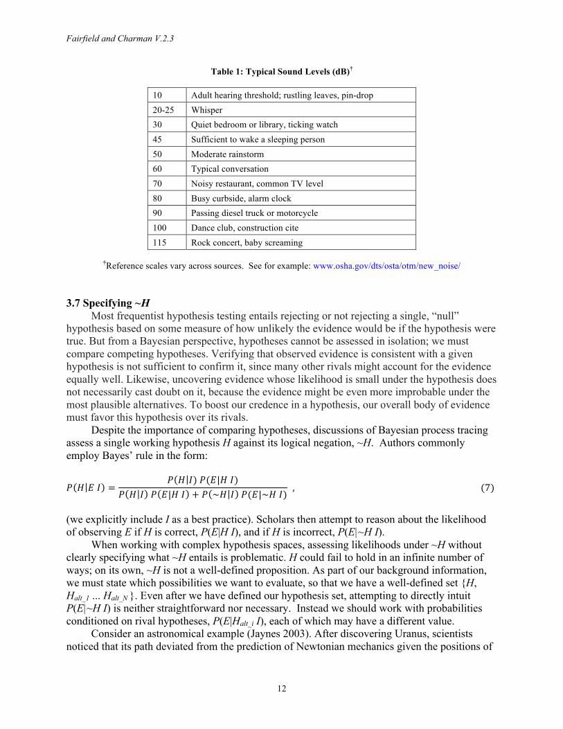
Measuring log-odds in decibels allows us to leverage our everyday experience with sound, while providing a quantitative underpinning for Gull’s metaphor of Bayesian inference as a dialogue with the data—in essence we can ask whether the evidence is whispering or shouting in favor of a particular hypothesis. In acoustics, the minimal noticeable change in ambient environments is roughly 3 decibels. A change of 5 decibels is clearly noticeable, while an increase of 10 decibels is perceived as about twice as loud; 20 decibels is roughly four times louder. Table 1 provides typical reference sounds in decibels. For example, a quiet bedroom averages 30 decibels, while an ordinary conversation is about 60 decibels.
When formalizing qualitative research, we suggest regarding decisive evidence that strongly favors one hypothesis over a rival as roughly equivalent to 30 decibels, which corresponds to the difference between a quiet bedroom and a conversation—in other words, the data are “talking clearly.” Likewise, a very low prior log-odds against a hypothesis relative to a more plausible rival could reasonably be set at –50 decibels (Jaynes 2003:99-100), the difference between a pin drop and a conversation.
In closing, we might remind readers who remain skeptical of working with decibels that use of a logarithmic scale for measuring odds ratios was a key insight that allowed Alan Turing to decode the German Enigma cypher, helping to secure an Allied victory in World War II.
Fairfield and Charman V.2.3
12
Table 1: Typical Sound Levels (dB)†
10 Adult hearing threshold; rustling leaves, pin-drop 20-25 Whisper 30 Quiet bedroom or library, ticking watch 45 Sufficient to wake a sleeping person 50 Moderate rainstorm 60 Typical conversation 70 Noisy restaurant, common TV level 80 Busy curbside, alarm clock 90 Passing diesel truck or motorcycle 100 Dance club, construction cite 115 Rock concert, baby screaming
†Reference scales vary across sources. See for example: www.osha.gov/dts/osta/otm/new_noise/
3.7 Specifying ~H
Most frequentist hypothesis testing entails rejecting or not rejecting a single, “null” hypothesis based on some measure of how unlikely the evidence would be if the hypothesis were true. But from a Bayesian perspective, hypotheses cannot be assessed in isolation; we must compare competing hypotheses. Verifying that observed evidence is consistent with a given hypothesis is not sufficient to confirm it, since many other rivals might account for the evidence equally well. Likewise, uncovering evidence whose likelihood is small under the hypothesis does not necessarily cast doubt on it, because the evidence might be even more improbable under the most plausible alternatives. To boost our credence in a hypothesis, our overall body of evidence must favor this hypothesis over its rivals.
Despite the importance of comparing hypotheses, discussions of Bayesian process tracing assess a single working hypothesis H against its logical negation, ~H. Authors commonly employ Bayes’ rule in the form:
𝑃 𝐻 𝐸 𝐼 =𝑃 𝐻 𝐼) 𝑃(𝐸|𝐻 𝐼)
𝑃 𝐻 𝐼 𝑃 𝐸|𝐻 𝐼 + 𝑃 ~𝐻 𝐼 𝑃(𝐸|~𝐻 𝐼) , (7)
(we explicitly include I as a best practice). Scholars then attempt to reason about the likelihood of observing E if H is correct, P(E|H I), and if H is incorrect, P(E|~H I).
When working with complex hypothesis spaces, assessing likelihoods under ~H without clearly specifying what ~H entails is problematic. H could fail to hold in an infinite number of ways; on its own, ~H is not a well-defined proposition. As part of our background information, we must state which possibilities we want to evaluate, so that we have a well-defined set {H, Halt_1 ... Halt_N }. Even after we have defined our hypothesis set, attempting to directly intuit P(E|~H I) is neither straightforward nor necessary. Instead we should work with probabilities conditioned on rival hypotheses, P(E|Halt_i I), each of which may have a different value.
Consider an astronomical example (Jaynes 2003). After discovering Uranus, scientists noticed that its path deviated from the prediction of Newtonian mechanics given the positions of
Fairfield and Charman V.2.3
13
the other astronomical bodies known at the time. The deviation could be reconciled by the presence of an as-yet undiscovered planet exerting a gravitation pull on Uranus. Neptune was subsequently found close to but not exactly at the predicted position. What does this discovery tell us about Newton’s theory (HN)? Jaynes (2003:135) emphasizes that we cannot assess the proposition that HN is correct against the proposition that it is incorrect, ~HN, because “the statement ‘Newton’s theory is false’ has no definite implications until we specify what alternative we have to put in place of Newton’s theory.” If the only alternative theory available at the time implied that no planets could exist beyond Uranus, then the likelihood of the evidence (Neptune’s measured location) under ~HN would be zero, and the discovery of Neptune would confirm HN, even though Neptune’s position was slightly off of the prediction. However, if the alternative theory is general relativity, the likelihood of the evidence under ~HN is the same as the likelihood under HN, since Einstein’s and Newton’s predictions do not differ detectibly in the case at hand, and we would have no cause to update our beliefs. The lesson is that:
Unless the observed facts are absolutely impossible on hypothesis H0, it is meaningless to ask how much those facts tend ‘in themselves’ to confirm or refute H0. ...we have not asked any definite, well-posed question until we specify the possible alternative to H0. Then... probability theory can tell us how our hypothesis fares relative to the alternatives we have specified. (Jaynes 2003:136)
Returning to political science, Bennett’s (2015) discussion of Tannenwald (2007) illustrates the potential problems of comparing H directly against ~H. As discussed previously, Bennett places a prior of 0.4 on Tannenwald’s taboo hypothesis, HT, regarding the non-use of nuclear weapons, and 0.6 on ~HT. Bennett (2015:279) then considers evidence E: “normative constraints were discussed” by decision-makers. Bennett reasons that P(E|HT) will be high and assigns a value of 0.9, conditional on the assumption that “we have access to evidence on the decision meetings.” In contrast, Bennett (2015:280) sets P(E|~HT) = 0.7, reasoning that decision-makers may have strategic reasons to publicly appeal to norms even if they reject use of nuclear weapons for other reasons: “A leader might cite his or her ‘principled’ restraint in not using nuclear weapons ...when in fact he or she was deterred by the threat of retaliation. Also, leaders might discuss normative constraints, but not make them the deciding factor if the military utility of nuclear weapons is in doubt.” Bennett thus calculates P(~HT) P(E|~HT) =0.6 × 0.7 =0.42, and P(HT) P(E|HT) =0.4 × 0.9 =0.36. Applying equation (5), he derives a posterior P(HT|E ) =0.46, slightly higher than his prior for the taboo hypothesis.
However, if we proceed more carefully by conditioning on a single alternative hypothesis at a time, we may arrive at a different posterior on the taboo hypothesis. Recall that Tannenwald specifies two main alternatives: HD = deterrence, and HM = military non-utility. We think the likelihood P(E|HM) should be lower than the likelihood P(E|HD). Whereas leaders may have instrumental reasons to display principled restraint rather than publicly admitting fear of retaliation and appearing weak relative to the enemy, we anticipate fewer incentives for leaders to make a show of principled restraint if they simply judge nuclear weapons to be militarily ineffective.16 We might therefore take P(E|HM) =0.3 and P(E|HD ) =0.7 (retaining Bennett’s linear probability scale to facilitate comparison). Taking Bennett’s prior of 0.4 on HT and his likelihood P(E|HT) =0.9, applying equal priors of 0.3 on HD and HM for lack of any better rationale, and substituting into Bayes theorem with each rival hypothesis specified in the denominator: 16 We are hardly experts, and I (suppressed in equations above following Bennett’s exposition) will play an important role in reasoning about these likelihoods.
Fairfield and Charman V.2.3
14
𝑃 𝐻! 𝐸 =𝑃(𝐻!) 𝑃(𝐸|𝐻!)
𝑃(𝐻!) 𝑃 𝐸|𝐻! + 𝑃(𝐻!) 𝑃 𝐸 𝐻! + 𝑃(𝐻!) 𝑃(𝐸|𝐻!) , (8)
we calculate P(HT|E) =0.54, which is higher than Bennett’s posterior of 0.46.
In sum, we must explicitly elaborate a set of mutually-exclusive alternatives to H in order to reason meaningfully about likelihoods if H does not hold. If there is more than one reasonable alternative hypothesis, this approach is especially critical. 3.8 Focusing on the Fundamentals
If we simply wish to assess explanations, formal Bayesian process tracing requires specifying nothing more than priors and likelihoods. Additional complications found in the literature—ad-hoc probability rules, extensive parameterizations, or classifications of evidence and test types—are at best unnecessary.
Several scholars introduce additional probabilities that we view as incorrect extensions of Bayesian logic. Beach and Pedersen (2013:126-29) propose assessing the probability that the “evidence” is “accurate” as an additional, distinct component of Bayesian analysis. In their approach, if a source provides information X, then X is considered to be the evidence. Instead, we advocate directly evaluating the likelihood that a particular source would make statement X, given the specific hypothesis under consideration and the background information, which includes assessments of the source’s reliability and other relevant contextual information. This approach—defining E as “source S says X”—is not only simpler, it is also analytically imperative, because in general the accuracy of information X depends on the hypothesis under consideration (Appendix 1). Kreuzer and DeFina (2015) propose the notion of “evidentiary fit” to assess how well a piece of evidence matches a theoretical prediction; they use this new probability as a “discount factor” applied to the likelihood. However, the likelihood, if correctly specified and evaluated, is precisely what tells us how well the evidence fits with the hypothesis, and likelihood ratios indicate how much the evidence discriminates between different hypotheses. The tendency to create ad hoc rules is widespread in subjective Bayesian probability literature; however, Cox’s axioms imply that any proposed additions or extensions will either reproduce the basic formalism or inevitably produce inconsistencies (Jaynes 2003).
If our goal is applying Bayesian analysis to evidence-intensive process-tracing, Humphreys and Jacobs’ (2015) innovative Bayesian model for multimethod research (BIQQ)—designed to combine correlational data with process-tracing “clues”—is also more complicated than needed. Drawing on medical testing analogies, they classify cases into types (adverse, beneficial, chronic, destined) according to the potential outcome a “treatment” would elicit. Because these types are unobservable and carry no information about causal mechanisms, we regard them as nuisance parameters. This setup becomes cumbersome if we are dealing with a single case and searching for the best explanation of an outcome that actually occurred, rather than assessing population-level parameters from a sample. Instead of conditioning on the case’s hidden type, we can directly evaluate the likelihood of observing the evidence conditional on each hypothesis we wish to compare, which is much closer to how process tracers approach inference. Although Humphreys and Jacobs outline extensions of their model that accommodate theory comparison, they do so in a way that retains the emphasis on proportions of types within a population, whereas in our more fully Bayesian approach, causal hypotheses for explaining the known outcome of a given case are the primary propositions of interest. Moreover, the number of BIQQ
Fairfield and Charman V.2.3
15
model parameters grows rapidly as competing causal hypotheses, treatments, potential outcomes, and the number and complexity of process-tracing clues increase. Specifying, let along computing, the requisite parameters would be unwieldy for in-depth case analysis.
We further emphasize that the type of evidence—however distinctions are delimited—does not matter for the fundamental logic of Bayesian analysis (although the difficulty of assigning probabilities may vary). Evidence may include “causal-process observations” about mechanisms, or “data-set observations” with scores on dependent and independent variables (Collier, Brady, and Seawright 2010); relatedly, “within-case” observations (Bennett and Checkel 2015:8), or cross-case observations. Evidence may contain information about timing and sequencing, or other aspects of causal mechanisms; obtained from archival sources, or interviews. Regardless, Bayesian analysis entails evaluating likelihoods—stated more strongly, the evidence enters our calculations only through likelihoods. Classification of evidence is beside the point unless it helps us evaluate likelihoods. We therefore suspect that categorizing types of process-tracing evidence (Beach and Pedersen 2013:99-100) may make a limited contribution to elucidating inference. In accord with this view, Collier (2011) simply focuses on “diagnostic evidence”—which we interpret to mean evidence for which the likelihood varies across hypotheses—as the key to process tracing. We add that diagnostic evidence underpins all scientific inference.
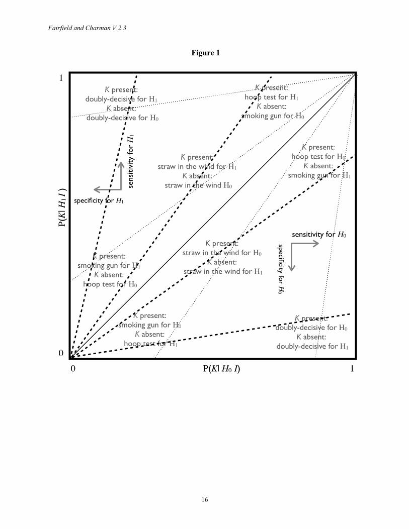
Typologies of test strength are also unnecessary, because confirmation is always a matter of degree and is always effected using Bayes’ theorem. Recent scholarship endeavors to give Van Evera’s (1997) process-tracing tests (smoking-gun, hoop, doubly-decisive, straw-in-the-wind) a Bayesian interpretation by replacing the common categorization based on uniqueness and certainty (or necessity and sufficiency) with specificity and sensitivity (Humphreys and Jacobs 2015, Bennett 2015). While probabilistic understandings were also present in earlier treatments (Van Evera 1997, Collier 2011, Mahoney 2012), specificity and sensitivity are more naturally probabilistic terms. However, when we move away from the limiting case of deductive logic, specificity and sensitivity do not yield a sensible classification of tests. Consider Figure 1, which displays Humphreys and Jacobs’ (2015:13) mapping of test types onto “probative value” space, defined by the likelihood of observing a clue K under a hypothesis H0 and under a rival H1. Notice that all points along any given line drawn from the origin correspond to evidence producing the same likelihood ratio when K is found, and hence tests of equal strength that lead to identical updating. Test strength increases as the slope of these lines diverges from the 45-degree diagonal. The dashed lines in Figure 1 show that clues located in distinct test-type regions can all have equal strength. Furthermore, small differences in location near the origin generate tests of extremely different strengths, whereas Humphreys and Jacobs’ mapping suggests that all evidence in this neighborhood is smoking-gun like. While process-tracing tests have made a major contribution to qualitative methods, we advocate focusing on likelihood ratios and simply following the universal Bayesian procedure for updating probabilities. If test types are still desired, they should be based on either weight of evidence or relative entropy (Appendix 2).
Fairfield and Charman V.2.3
16
Figure 1
K present:smoking gun for H1
K absent: hoop test for H0
K present:doubly-decisive for H1
K absent: doubly-decisive for H0
K present:straw in the wind for H1
K absent: straw in the wind H0
K present:hoop test for H1K absent:
smoking gun for H0
K present:smoking gun for H0
K absent: hoop test for H1
K present:doubly-decisive for H0
K absent: doubly-decisive for H1
K present:hoop test for H0K absent:
smoking gun for H1
K present:straw in the wind for H0
K absent: straw in the wind for H1
P(K| H0 I)
sens
itivi
ty fo
r H
1
specificity for H1
sensitivity for H0
specificity for H0
P(K
| H1 I )
0 10
1
Fairfield and Charman V.2.3
17
3.9 Empirical Example Appendix 3 applies our best practices to formalize a case study from Fairfield’s (2015)
research on tax policy change in Latin America. The case—elimination of a regressive tax benefit in Chile in 2005—was previously analyzed with both the traditional narrative approach and explicit application of process-tracing tests (Fairfield 2013) and therefore facilitates methodological comparison with Bayesian analysis. Other efforts to formalize Bayesian process tracing examine only a few illustrative pieces of evidence (Rohlfing 2013, Bennett 2015) and/or include only highly simplified process-tracing observations (Humphreys and Jacobs 2015).
We compare Fairfield’s explanation for why the tax reform was approved against three rival hypotheses in light of six key observations from the case narrative. We assign likelihoods to each piece of evidence, conditioning not only on the background information and the hypothesis under consideration, but also on previously-incorporated evidence that may be dependent. In assessing likelihoods conditional on each hypothesis, we also carefully consider potential instrumental incentives and biases among sources. We then assess the strength of the inference jointly derived from the six pieces of evidence and engage in Bayesian sensitivity analysis to ascertain how much the conclusions depend on choices of priors and values assigned to likelihood ratios. The exercise illustrates how a decibel scale in conjunction with our sound analogy facilitates intuitive assignments for the weight of evidence and ensures as much consistency as possible when quantifying inherently qualitative information.
4. Pros and Cons of Formalization In the context of efforts to establish process tracing as a rigorous methodology and growing
attention to analytical transparency, scholars have advocated formalizing Bayesian analysis to make inferences more systematic, explicit, and amenable to scrutiny (Rohlfing 2013; Bennett and Checkel 2015:267; Bennett 2015:297; Humphreys and Jacobs 2015). Formalization forces us to clearly identify and carefully consider all salient evidence. It precludes focusing exclusively on a working hypothesis by requiring us to consider states of the world characterized by rival hypotheses. Formalization may also “eliminate the considerable ambiguity in many verbal phrases used to convey probabilities” (Bennett 2015:297). Moreover, formalization holds out the possibility of allowing us to analyze and aggregate complex evidence more systematically than intuition alone would permit. However, Appendix 3 illustrates that formalization is indeed a “very tall order” (Humphreys and Jacobs 2015:42) for evidence-intensive process tracing. As such, we must assess both anticipated benefits and potential drawbacks. We begin by discussing caveats based on our experience of elaborating Appendix 3 and then consider situations where formalization can be valuable despite the challenges.
4.1 Caveats and Limitations
The foremost challenge of formalization entails assigning numerical values to all probabilities (priors and likelihoods). This task is problematic when the data are inherently qualitative. Our likelihood values required multiple rounds of revision before they became reasonably stable and mutually consistent, and there is no guarantee that we would have arrived at the same values had we initially approached the problem using a different sequencing of the evidence, or that we would produce at similar values upon redoing the analysis from scratch. We view this issue as a fundamental problem that cannot easily be resolved. Specifying a range of probabilities rather than a precise value (Humphreys and Jacobs 2015) merely relocates the
Fairfield and Charman V.2.3
18
arbitrariness of quantification.17 While words used to express probability in common parlance are certainly ambiguous, quantification may simply disguise that ambiguity with false precision.18
Although we may be inclined to view formal Bayesian analysis as more rigorous than informal inference, the arbitrariness of quantification in qualitative research must give us pause. In cases where formalization leads to conclusions that differ from informal analysis, there is no way to objectively assess whether those conclusions are better or more correct. Assigning numbers does not eliminate subjectivity and intuition; it merely changes how we use our intuition. Ultimately, we have only intuition to guide us in judging the quality of inferences, whether formal or informal.
Second, formal Bayesian analysis becomes intractable beyond very simple causal models, which are rarely adequate in social science. Recall that formal analysis usually entails specifying mutually-exclusive hypotheses, which is nontrivial and may require over-simplification. Some of the hypotheses assessed against Fairfield’s (2013) explanation in Appendix 3 involve causal mechanisms that—in the real world—could potentially operate simultaneously or in interaction. Assessing such possibilities requires carefully elaborating additional, more complex mutually-exclusive hypotheses and would aggravate the challenges of quantifying likelihoods. By contrast, in the natural sciences, Bayesian analysis is usually applied to very simple hypothesis spaces (even if the underlying theory and experiments are highly complex); for example: H1 = the Higgs boson mass is 124–126 GeV/c2, H2 = the mass is 126–128 GeV/c2, etc.
Third, practical considerations preclude widespread application of formal Bayesian analysis in process tracing research. Appendix 3 exceeds the full length of Fairfield’s (2013) article, which included three additional case studies. We cannot expect scholars to formalize all of their cases without producing heavy disincentives for process tracing.
Finally, formalization should not be equated with transparency. On the one hand, formal analysis can obscure rather than clarify inference, especially if we disaggregate the evidence too finely and unpack our analysis into too many steps—we may become lost in minutiae. Moreover, making too many steps explicit may lull readers into uncritically accepting the author’s reasoning, rather than assessing whether they can arrive at the conclusions through their own independent logical pathways, thereby undermining the scholarly scrutiny of inferences that analytical transparency is intended to promote. Even mathematicians routinely skip steps in proofs; readers must fill in and verify themselves, which provides an important cross-check. On the other hand, transparency does not require quantification for mathematical application of Bayes’ theorem. Scholars can make the assumptions and logic behind their inferences explicit without numbers. In other words, we see the issue of clarifying assumptions and explaining the rationale underpinning nuanced inferences as distinct from the question of formalization, which entails moving qualitative research into the realm of quantitative research. While these considerations do not necessarily constitute an argument against formalization, they clarify that transparency is not necessarily an argument for formalization.
17 To avoid subjective likelihood assignments, Humphreys and Jacobs (2015) include priors on the probative value of process-tracing clues; yet the problem then becomes how to translate background knowledge and theoretical expectations into an appropriate prior distribution. Moreover, if we work within a single case, only averages over priors for clue probabilities matter, so their approach reduces to specifying likelihoods. 18 Capoccia and Kelemen (2007:362) similarly note: “While historical arguments relied on assessments of the likelihood of various outcomes, it is obviously problematic to assign precise probabilities.”
Fairfield and Charman V.2.3
19
4.2 Applications Given the caveats, when might formal Bayesian analysis prove most useful? Regarding
which cases to formalize, the value will depend on the evidence. If all observations strongly favor a particular hypothesis, formalization is unlikely to improve on intuition. Scholars can explain why the evidence is decisive without quantifying probabilities, and if the evidence is indeed decisive, readers should recognize it as such on its face. Likewise, if the evidence has weak probative value, formalization may simply confirm the realization we would have obtained intuitively—the evidence is insufficient to strongly support any particular hypothesis (unless we already had strong priors or cannot think of reasonable alternatives).
The greatest potential gains for inference would arise when the evidence is complex and does not clearly favor one hypothesis. Formalization would ideally help us keep track of nuances, consistently assess the weight of evidence for each observation, and systematically aggregate inferences across individual observations. These are precisely the situations where using Bayes’ theorem to move from attempting to directly evaluate P(H |E1–N I ) to instead assessing each P(Ex |H E1–x I )—some Ex’s might fit the hypothesis better than others—would in theory be most helpful for leveraging our intuition.
However, there is a danger when evidence is ambivalent that conclusions derived via formalization may simply be driven by arbitrariness inherent in quantification of qualitative evidence. Physicists would only believe that noisy data accumulates into a significant signal if the error model is well understood; in qualitative social science, analogous situations may rarely arise. Almost by definition, if the evidence pulls in different directions, small changes in probabilities may swing the inference in favor of one hypothesis or another. Ironically then, the cases where formalization ostensibly offers the most leverage are those where it may be most vulnerable to arbitrary quantification.
Nevertheless, formalization in such cases might be merited for the sake of analytical transparency and informing future research decisions. Regarding transparency, if we must make inferential claims on the basis of ambivalent or weak evidence—if important questions are at stake19 and obtaining better evidence is infeasible—formal analysis could at least clarify the basis on which those claims rest and facilitate debate among scholars. Looking forward to future data-gathering opportunities, formalization might also help elucidate what kind of additional evidence would be most valuable for strengthening the inference.
We envision a more important role for formalization in identifying the locus of contention when scholars disagree on inferences. As Hunter (1984:88) argues, through formalization, “the sources of the disagreement can be determined much more easily than in normal verbal analysis.” Formal Bayesian analysis provides a clear framework for pinpointing disagreements: Do they arise from different background information and assumptions (e.g. a source’s motives or sincerity), different priors, or different assessments of likelihoods? If the problem lies with the probative value of evidence, which observations are most contested and why? For these purposes, numbers serve primarily to stimulate discussion about inferential logic, assumptions, and judgments, and the ad-hoc component of quantification may be less problematic.
We explore how this clarification and adjudication process might work in Appendix 3. We assign three sets of priors corresponding to different initial probabilities on Fairfield’s (2013) explanation and three rivals. For each prior, we calculate posterior probabilities across scenarios where we assign larger or smaller likelihood ratios for the evidence. This Bayesian sensitivity analysis reveals that to remain unconvinced, a skeptical reader would need to have extremely 19 Hunter (1984) explores military applications.
Fairfield and Charman V.2.3
20
strong priors against Fairfield’s explanation and/or contend that the evidence is far less discriminating than we have argued (Section A3.5).
We also foresee a valuable pedagogical role for formalization. Reading examples and conducting exercises could familiarize practitioners with Bayesian probability and train intuition to follow this inferential logic more systematically, thereby improving informal process tracing. For example, one of the most salient lessons from Appendix 3 is that the weight of evidence depends by definition on which hypotheses we compare; we cannot judge how decisive the evidence is with respect to our working hypothesis alone, without considering concrete alternatives. Thinking in these terms, even without quantifying probabilities, may help scholars identify and deploy their most discriminating observations in case narratives. Appendix 3 also demonstrates that the accuracy of a source cannot be assessed a priori. Even if we trust an informant, under some hypotheses, the statements s/he has made may necessarily be untrue.
Relatedly, elaborating a formal Bayesian appendix for an illustrative case from one’s own research might help establish process-tracing “credentials.” As much as we try to make our analysis transparent, multiple analytical steps will inevitably remain implicit. Qualitative research draws on vast amounts of data, often accumulated over multiple years of fieldwork. There is simply too much evidence and too much background information that informs how evidence is evaluated to fully articulate or catalog. Qualitative research is not replicable as per a laboratory science desideratum; at some level, we must trust that scholars have made sound judgments. To that end, scholars might use a formal illustration to demonstrate their care in reasoning about the evidence and the inferences it permits. 4.3 Informal Process-Tracing
When formal Bayesian analysis is not feasible, there is ample scope to improve inference and transparency in traditional narrative-based process tracing. Various recommendations following from points discussed in Section 3 can contribute to that end. We should begin by identifying the most plausible rival hypotheses and explaining why our background information from the outset suggests that some are more likely, or justifies disregarding relevant alternatives that are prevalent in the literature. When drawing inferences, we should identify key elements of the background information that are not common knowledge and explain how they inform our judgments. We should also include enough “thick description” of context and case details beyond the key evidence and background information for readers to evaluate alternative hypotheses that may not have occurred to us or that we deemed not plausible enough to merit explicit consideration. For example, the preference-change hypothesis evaluated in Appendix 3 appears reasonable on its face, and in retrospect the case narrative could have benefited from explicitly assessing that possibility; however, the text included sufficient information for readers to independently evaluate and discount that hypothesis. The ease of providing thick description is an advantage of narrative process tracing over formalization, where only information relevant to inferences on the designated hypothesis set would be catalogued.
These recommendations are not novel; after all, Bayesian probability “is nothing more than common sense reduced to calculation,” (Laplace, in Sivia 2006:13). Similar guidelines have been elaborated elsewhere (Bennett and Checkel 2015) and are reflected in longstanding exemplars of excellence in qualitative research (Wood 2000, Tannenwald 2007). Our point is to reiterate the importance of these recommendations, which are not always followed, and to emphasize their critical but not always appreciated methodological grounding in Bayesian probability.
Fairfield and Charman V.2.3
21
Some of the less widely-recognized points in Sections 3 also apply to informal process tracing. As in formal analysis, when working with documents, news sources, and interviews, informal process-tracers should take as evidence not the content of a statement, but the fact that a particular source made the statement; the next step is considering how the source’s potential biases and instrumental incentives might change under alternative hypotheses when assessing whether the evidence favors a particular explanation. Informal process-tracers should also be aware that contrary to conventional wisdom, distinct sources do not necessarily ensure logically independent evidence. Thinking carefully about logical dependence may be helpful for identifying the most discriminating pieces of evidence to showcase in space-constrained narratives. Perhaps most importantly, our sound analogy may aid intuition and reduce ambiguity when describing probabilities. Terms like “highly unlikely” or “plausible” may be interpreted very differently across individuals. In contrast, the sound analogy could establish better intersubjective agreement, because it is grounded in universal, concrete, everyday experience.
5. Conclusion
Bayesian analysis provides a critical methodological foundation for process tracing, a common mode of research that is incompatible with frequentistism. Bayesian probability allows us to directly ask how plausible a hypothesis is in light of the evidence, facilitates learning and knowledge accumulation, and permits inferences from a limited number of observations and/or cases. However, we have identified omissions and shortcomings in the nascent Bayesian process-tracing literature that arise from incomplete understandings of Bayesian probability.
With respect to formal Bayesian process tracing, our suggested best practices (Table 2) can help scholars proceed more consistently and more rigorously. While operationalizing Bayesian analysis is challenging, formalization may be especially valuable for pinpointing the locus of disagreements when inferences are contested and for training our reasoning to more closely approximate the Bayesian ideal.
However, we caution against a precipitous move toward quantifying qualitative research. Narrative-based process tracing has provided a wealth of knowledge and insights that have informed all realms of political science, and imposing a bar as high as formal Bayesian analysis could create strong disincentives for scholarship in this tradition, with potentially limited returns given arbitrariness in quantification. Considering that Bayesian probability is an aspirational goal for rational inference, when assessing complex evidence and explanatory hypotheses in social science, we may need to accept a more intuitive, qualitative approach. Even in the natural sciences, the most ardent advocate of Bayesian probability as extended logic maintained that “in practice, the situation faced by the scientist is so complicated that there is little hope of applying Bayes’ theorem to give quantitative results about the relative status of theories. And there is no need... common sense is quite adequate for that,” (Jaynes 2003:139).
We further emphasize that many insights from formal Bayesian analysis have implications for the informal, qualitative Bayesianism underlying narrative-based process tracing (Table 2). Whether or not scholars decide to formalize, understanding Bayesian probability can help avoid pitfalls such as failing to consider whether evidence that ostensibly supports a preferred hypothesis fits better with rivals, or assuming that distinct sources ensure independent evidence.
Investigating whether there is fruitful middle ground between informal and formal Bayesian process tracing is an important direction for future research. Thinking in terms of a continuum may be helpful. As we move from informal analysis toward what might be called “semi-formal” analysis, we would begin to use the language of probability more explicitly (but
Fairfield and Charman V.2.3
22
without using the mathematics of probability). We might make qualitative use of the sound analogy, communicating relative probabilities by asking “how loudly the data are talking.” As we progress further toward the formal end of the continuum, we might use sound reference levels (e.g. the data speak in favor of H1 over H2 at a conversational level). Moving closer toward formalization, we might specify the corresponding decibels for the most cogent evidence, particularly if it helps us think more explicitly about non-trivial assumptions and reveal background information that matters for our judgments. Numbers employed in this type of semi-formal analysis—without conducting the various internal consistency checks on probability assignments necessary for formal analysis—should be viewed only as a way to effectively communicate analytical judgments and a stimulus for thinking carefully about the evidence. Full formalization (Appendix 3) entails systematically quantifying all probabilities and applying Bayes’ theorem to derive an aggregate inference.
Moving forward, scholars will need to ascertain where the optimal point on this continuum lies. It may vary depending on characteristics of the research (e.g. quality of evidence, complexity and number of salient hypotheses), as well as how controversial the inferences prove. A logical first step, which we are currently undertaking in a related project, entails investigating how much inferences change when scholars reason formally as opposed to informally (Bennett 2015:297). In Appendix 3, we did not discover any instances where formal Bayesian analysis diverged from the original case narrative’s conclusions. This consistency could indicate that informal reasoning functioned well, or that the intuition underpinning that informal analysis also strongly shaped quantification decisions. Whether formal analysis on a case with less decisive evidence would produce different conclusions compared to informal analysis remains an open question. Beyond analyzing whether inferences differ, we also need to ask how compelling the research community finds conclusions reached from informal vs. formal or semi-informal analysis, and whether the latter approaches facilitate consensus-building.
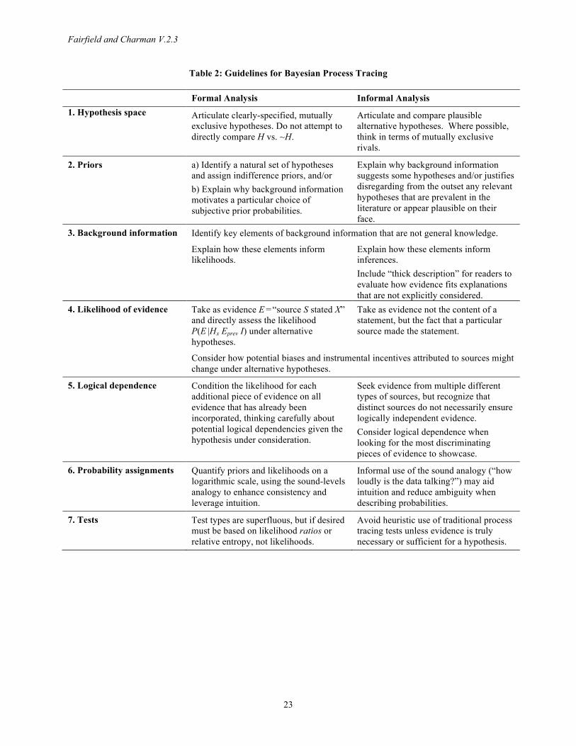
Fairfield and Charman V.2.3
23
Table 2: Guidelines for Bayesian Process Tracing
Formal Analysis Informal Analysis 1. Hypothesis space Articulate clearly-specified, mutually
exclusive hypotheses. Do not attempt to directly compare H vs. ~H.
Articulate and compare plausible alternative hypotheses. Where possible, think in terms of mutually exclusive rivals.
2. Priors a) Identify a natural set of hypotheses and assign indifference priors, and/or b) Explain why background information motivates a particular choice of subjective prior probabilities.
Explain why background information suggests some hypotheses and/or justifies disregarding from the outset any relevant hypotheses that are prevalent in the literature or appear plausible on their face.
3. Background information Identify key elements of background information that are not general knowledge.
Explain how these elements inform likelihoods.
Explain how these elements inform inferences. Include “thick description” for readers to evaluate how evidence fits explanations that are not explicitly considered.
4. Likelihood of evidence Take as evidence E =“source S stated X” and directly assess the likelihood P(E |Hx Eprev I) under alternative hypotheses.
Take as evidence not the content of a statement, but the fact that a particular source made the statement.
Consider how potential biases and instrumental incentives attributed to sources might change under alternative hypotheses.
5. Logical dependence Condition the likelihood for each additional piece of evidence on all evidence that has already been incorporated, thinking carefully about potential logical dependencies given the hypothesis under consideration.
Seek evidence from multiple different types of sources, but recognize that distinct sources do not necessarily ensure logically independent evidence. Consider logical dependence when looking for the most discriminating pieces of evidence to showcase.
6. Probability assignments Quantify priors and likelihoods on a logarithmic scale, using the sound-levels analogy to enhance consistency and leverage intuition.
Informal use of the sound analogy (“how loudly is the data talking?”) may aid intuition and reduce ambiguity when describing probabilities.
7. Tests Test types are superfluous, but if desired must be based on likelihood ratios or relative entropy, not likelihoods.
Avoid heuristic use of traditional process tracing tests unless evidence is truly necessary or sufficient for a hypothesis.
Fairfield and Charman V.2.3
24
References APSA. 2012. A Guide to Professional Ethics in Political Science, Second Edition. American
Political Science Association. Beach, Derek, and Rasmus Pedersen. 2013. Process-Tracing Methods. University of Michigan
Press. –––––. 2014. “Let the evidence speak.” Annual Conference of the American Political Science
Association, Washington, DC. Bennett, Andrew. 2008. “Process Tracing: A Bayesian Perspective.” In Janet Box-
Steffensmeier, Henry Brady, and David Collier, eds, The Oxford Handbook of Political Methodology, Oxford University Press, 702-721.
_____. 2015. “Disciplining Our Conjectures: Systematizing Process Tracing with Bayesian Analysis.” In Andrew Bennett and Jeffrey Checkel, eds, Process Tracing in the Social Sciences: From Metaphor to Analytic Tool. Cambridge University Press, 276–98.
Bennett, Andrew, and Jeffrey Checkel, eds. 2015. Process Tracing in the Social Sciences: From Metaphor to Analytic Tool. Cambridge University Press.
Capoccia, Giovanni, and R. Daniel Kelemen. 2007. “The Study of Citical Junctures.” World Politics 59 (April): 341-69.
Collier, David. 2011. “Understanding Process Tracing,” PS: Political Science and Politics 44 (4): 823–30.
Cox, Richard. 1961. The Algebra of Probable Inference. Johns Hopkins University Press. Fairfield, Tasha. 2013. “Going Where the Money Is: Strategies for Taxing Economic Elites in
Unequal Democracies.” World Development 47: 42–57. –––––. 2015. Private Wealth and Public Revenue in Latin America: Business Power and Tax
Politics. Cambridge University Press. Gelman, Andrew, John Carlin, Hal Stern, David Dunson, Aki Vehtari, and Donald Rubin. 2013.
Bayesian Data Analysis, Third Edition. CRC Press. Gill, Jeff. 2008. Bayesian Methods: A Social and Behavioral Sciences Approach. Taylor and
Francis. Gill, Jeff, and Christopher Witko. 2013. “Bayesian Analytical Methods: A Methodological
Prescription for Public Administration,” Journal of Public Administration Research and Theory 23 (2): 457-494.
Good, I.J. 1985. “Weight of Evidence: A Brief Survey.” In J.M. Bernardo, M.H. de Groot, D.V. Lindley, and A.F.M. Smith, eds., Bayesian Statistics 2. New York: Elsevier.
Gregory, Phil. 2005. Bayesian Logical Data Analaysis for the Physical Science. Cambridge University Press.
Howson, Colin, and Peter Urbach. 2006. Scientific Reasoning: The Bayesian Approach. Caris Publishing Company.
Hunter, Douglas. 1984. Political/Military Applications of Bayesian Analysis. Boulder: Westview Press.
Humphreys, Macartan, and Alan Jacobs. Forthcoming. “Mixing Methods: A Bayesian Approach.” American Political Science Review.
Jackman, Simon. 2009. Bayesian Analysis for the Social Science. Wiley. Jaynes, E.T. 2003. Probability Theory: The Logic of Science. Cambridge University Press. Jeffery, Richard. 1983. The Logic of Decision. University of Chicago Press.
Fairfield and Charman V.2.3
25
Kreuzer, Marcus. 2010. “Historical Knowledge and Quantitative Analysis: The Case of the Origins of Proportional Representation.” American Political Science Review 104 (2): 369-92.
Kreuzer, Marcus, and Robert DeFina. 2015. “Look Before You Leap: The Hidden Historical Logic of Bayesian Analysis.” Annual Meeting of the American Political Science Association, San Francisco.
Mahoney, James. 2012. “The Logic of Process Tracing Tests in the Social Sciences.” Sociological Methods and Research 41: 570-97.
McKeown, Timothy. 1999. “Case Studies and the Statistical Worldview.” International Organization 53 (1): 161-190.
Rohlfing, Ingo. 2013. Case Studies and Causal Inference. Palgrave Macmillan. –––––. “Bayesian Causal Inference in Process Tracing: The Importance of Being Probably
Wrong.” Annual Meeting of the American Political Science Association, Chicago. Sivia, D.S., 2006. “Data Analysis—A Dialogue With The Data,” in Advanced Mathematical and
Computational Tools in Metrology VII, P. Ciarlini, E. Filipe, A.B. Forbes, F. Pavese, C. Perruchet and B. Siebert (eds.), World Scientific Publishing Co., 108-118.
Sivia, D.S., with J. Skilling. 2006. Data Analysis: A Bayesian Tutorial, 2nd Ed. New York: Oxford.
Stokes, Susan. 2001. Mandates and Democracy: Neoliberalism by Surprise in Latin America. Cambridge University Press.
Tannenwald, Nina. 2007. The Nuclear Taboo: The United States and the Non-Use of Nuclear Weapons since 1945. Cambridge University Press.
Van Evera, Stephen. 1997. Guide to Methods for Students of Political Science. Cornell University Press.
Van Fraassen, Bas. 1989. Laws and Symmetry. Oxford: Clarendon Press. Wood, Elisabeth. 2000. Forging Democracy from Below: Insurgent Transitions in South Africa
and El Salvador. Cambridge University Press.
Fairfield and Charman V.2.3
26
Appendices
A1. Evidence and Accuracy
Some scholars have attempted to articulate a notion of the accuracy of evidence for Bayesian analysis that assesses the reliability of the source independently of the hypotheses under consideration (Beach and Pedersen 2013:126-28, see also Bennett and Checkel 2015: 24-25).20 While this approach may be appropriate in some situations in the physical sciences where the accuracy of a measurement device does not depend on the hypothesis being tested, it may foster errors if applied to process tracing. We do not make separate assessments of the accuracy of information X provided by source S. Instead, we should directly evaluate the likelihood that “source A stated X,” given a particular hypothesis and our background information.
To illustrate, suppose E represents the evidence that informant S made a statement X (in some context C, for example, an interview with the author). Evaluating each likelihood P(E|Hi I) will require assessing the informant’s potential motives to assert X under a given hypothesis, as well as assessing the informant’s overall sincerity, knowledgeability, and judgment using the background information (independent of the hypotheses). In general, the accuracy of the statement X—which should be understood as the probability that X is true given that that the informant asserted it—depends on the hypothesis under consideration. The motives we attribute to the informant and hence the probability that s/he is speaking the truth may vary across hypotheses. Furthermore, it may be the case that a hypothesis directly implies that X is true, and hence the statement is accurate, regardless of whether we trust the informant more generally or whether we believe s/he is in a position to have correct information. Under a different hypothesis, we may ascertain that X cannot be true, in which case the statement is not accurate, and E must have occurred because the informant was either mistaken or lying. If we expand P(X|E I) using the assumption (contained in the background information) that we are considering mutually exclusive and exhaustive hypotheses H1-HN,
𝑃 𝑋 𝐸 𝐼 = 𝑃 𝑋 (𝐻1 + 𝐻2 +⋯+ 𝐻!) 𝐸 𝐼 = 𝑃 𝑋 𝐻1 𝐸 𝐼 +⋯+ 𝑃 𝑋 𝐻!|𝐸 𝐼
= 𝑃 𝑋 𝐸 𝐻1 𝐼 𝑃 𝐻1 𝐸 𝐼 +⋯+ 𝑃 𝑋 𝐻! 𝐸 𝐼 𝑃 𝐻! 𝐸 𝐼) , (𝐴1.1) where P(X|E Hi I) can be regarded as the hypothesis-dependent accuracy—the conditional probability that X is true given both that the informant asserted the statement E and that a particular hypothesis Hi holds. But note that we now have factors P(Hi |E I) which must be calculated using Bayes’ rule: P(Hi |E I) = P(E |Hi I) P(Hi |I) ⁄ P(E |I), and we are back to the task of assessing P(E |Hi I), which we can (and in practice must) do directly, without recourse to P(X |E I).
We can only move from assessing P(E |Hi I) to considering P(X |Hi I) in special cases where (a) we judge the accuracy of a statement to be very high across hypotheses, and (b) we judge incentives for the informant to reveal X if it is in fact the truth to be nearly the same across hypotheses. Suppose we wish to calculate likelihood ratios P(E |Hi I) ⁄ P(E |Hj I). Since X and ~X are mutually exclusive and exhaustive (X is either true or false),
20 Beach and Pedersen (2013: 127) base their discussion of the “accuracy of evidence” on Howson and Urbach’s (2006: 107-113) treatment of a very different problem—how evidence affects credence in primary and auxiliary hypotheses. However, Howson and Urbach’s example is not applicable to assessing the accuracy of sources in qualitative social science.
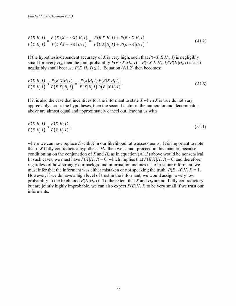
Fairfield and Charman V.2.3
27
𝑃 𝐸 𝐻! 𝐼𝑃 𝐸 𝐻! 𝐼
=𝑃 𝐸 𝑋 + ~𝑋 𝐻! 𝐼)𝑃 𝐸 𝑋 + ~𝑋 𝐻! 𝐼
= 𝑃 𝐸 𝑋 𝐻! 𝐼 + 𝑃 𝐸 ~𝑋 𝐻! 𝐼𝑃 𝐸 𝑋 𝐻! 𝐼 + 𝑃 𝐸 ~𝑋 𝐻! 𝐼
, (𝐴1.2)
If the hypothesis-dependent accuracy of X is very high, such that P(~X |E Hn, I) is negligibly small for every Hn, then the joint probability P(E ~X |Hn, I) = P(~X |E Hn, I)*P(E |Hn I) is also negligibly small because P(E |Hn I) ≤ 1. Equation (A1.2) then becomes: 𝑃 𝐸 𝐻! 𝐼𝑃 𝐸 𝐻! 𝐼
≈𝑃 𝐸 𝑋 𝐻! 𝐼)𝑃 𝐸 𝑋| 𝐻! 𝐼
= 𝑃 𝑋 𝐻! 𝐼 𝑃 𝐸 𝑋 𝐻! 𝐼𝑃 𝑋 𝐻! 𝐼 𝑃 𝐸 𝑋 𝐻! 𝐼
, (𝐴1.3)
If it is also the case that incentives for the informant to state X when X is true do not vary appreciably across the hypotheses, then the second factor in the numerator and denominator above are almost equal and approximately cancel out, leaving us with 𝑃 𝐸 𝐻! 𝐼𝑃 𝐸 𝐻! 𝐼
≈𝑃 𝑋 𝐻! 𝐼𝑃 𝑋 𝐻! 𝐼
, (𝐴1.4)
where we can now replace E with X in our likelihood ratio assessments. It is important to note that if X flatly contradicts a hypothesis Hn, then we cannot proceed in this manner, because conditioning on the conjunction of X and Hn as in equation (A1.3) above would be nonsensical. In such cases, we must have P(X |Hn I) = 0, which implies that P(E X |Hn I) = 0, and therefore, regardless of how strongly our background information inclines us to trust our informant, we must infer that the informant was either mistaken or not speaking the truth: P(E ~X |Hn I) = 1. However, if we do have a high level of trust in the informant, we would assign a very low probability to the likelihood P(E |Hn I). To the extent that X and Hn are not flatly contradictory but are jointly highly improbable, we can also expect P(E |Hn I) to be very small if we trust our informants.
Fairfield and Charman V.2.3
28
A2. Bayesian Test Types and Test Strengths
In the deterministic (deductive-logic) limit, Van Evera’s (1997) process-tracing tests can be used to compare two rival hypotheses (i.e. mutually exclusive and assumed exhaustive), H1 and H0, in light of a single clue, which can turn out to be present (K) or absent (~K).21 If the clue is certain to occur under H1, but is not unique to H1 (such that K is possible under H0),22 then searching for K entails a hoop test for H1. H1 passes the hoop test if the clue is found (lending mild support for H1) and fails if the clue is absent (refuting H1). A smoking-gun test for H1 involves a clue that is not certain under H1 but is unique to H1, such that the hypothesis passes if the clue is found (confirming H1) and fails otherwise (providing mildly disconfirming evidence for H1). A doubly-decisive test involves a clue that is both certain under and unique to H1, so that either clue outcome is decisive—the test acts simultaneously as a hoop and a smoking gun, confirming H1 and disconfirming H0. Notice that a hoop test for H1 with respect to K is a smoking gun test for H0 with respect to ~K, and vice-versa. Van Evera (1997) referred to instances where clue outcomes are neither certain nor unique as straw-in-the-wind tests that only mildly support or cast doubt on the hypotheses. In terms of informativeness, doubly-decisive tests are stronger than hoop and smoking-gun tests, which in turn are stronger than straw-in-the-wind tests. However, Van Evera did not provide a precise measure of test strength.
Van Evera and subsequent authors acknowledged that truly certain (necessary) or unique (sufficient) evidence is rare for complex hypotheses. For the test typology to be useful in practice, the notions of certainty and uniqueness must somehow be relaxed from absolute logical categories to matters of degree. Borrowing from the medical diagnostics literature, Bennett (2015:283) and Humphreys and Jacobs (2015) use the concepts of sensitivity and specificity, defined such that the test’s sensitivity to K under H1 is the likelihood P(K|H1 I), and the specificity of the test for H1 equals 1–P(K|H0 I).
However, in Section 3.8, we explained that these clue likelihoods are not a good way to generalize process-tracing tests to a fully probabilistic world where confirmation is a matter of degree. We showed that clues located in regions labeled by different test types in Humphreys and Jacobs’ probative-value space can all produce exactly the same updating. Further, while Humphreys and Jacobs (2015:68) recognize that: “a belief can gain support from data that are unlikely under that belief—as long as those data are even more unlikely under the alternatives,” their figure incorrectly suggests that all evidence in the neighborhood of the origin will be smoking-gun like, even though small differences in location near the origin actually generate tests of extremely different strengths.
Instead of likelihoods, we develop three Bayesian alternatives that are better suited for mapping process-tracing tests in “probative-value space”: (1) weights of evidence, (2) relative entropies, and (3) expected information gain. While we maintain that typologies of test strength are unnecessary, because we always update probabilities in the same way using Bayes theorem once the data are in hand, relative entropies and expected information gain may be of interest at the pre-data stage of research. However, the discussion below applies only when just two rival hypotheses are relevant to the problem and the evidence in question can sensibly be treated as binary.
21 More generally, we can work with any binary evidence that may assume one of two possible values or outcomes. 22 Instead of certainty and uniqueness, we can equivalently speak of clues that are necessary implications of or sufficient conditions for a hypothesis.
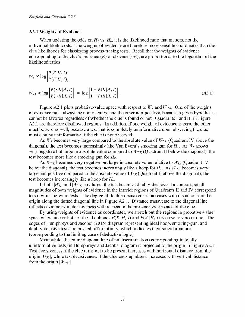
Fairfield and Charman V.2.3
29
A2.1 Weights of Evidence
When updating the odds on H1 vs. H0, it is the likelihood ratio that matters, not the individual likelihoods. The weights of evidence are therefore more sensible coordinates than the clue likelihoods for classifying process-tracing tests. Recall that the weights of evidence corresponding to the clue’s presence (K) or absence (~K), are proportional to the logarithm of the likelihood ratios:
𝑊! ∝ log𝑃 𝐾 𝐻o 𝐼𝑃(𝐾|𝐻o 𝐼)
𝑊~! ∝ log𝑃 ~𝐾 𝐻1 𝐼𝑃 ~𝐾 𝐻o 𝐼
= log1 − 𝑃 𝐾 𝐻1 𝐼1 − 𝑃 𝐾 𝐻o 𝐼
. (𝐴2.1)
Figure A2.1 plots probative-value space with respect to WK and W~K. One of the weights
of evidence must always be non-negative and the other non-positive, because a given hypotheses cannot be favored regardless of whether the clue is found or not. Quadrants I and III in Figure A2.1 are therefore disallowed regions. In addition, if one weight of evidence is zero, the other must be zero as well, because a test that is completely uninformative upon observing the clue must also be uninformative if the clue is not observed.
As WK becomes very large compared to the absolute value of W~K (Quadrant IV above the diagonal), the test becomes increasingly like Van Evera’s smoking gun for H1. As WK grows very negative but large in absolute value compared to W~K (Quadrant II below the diagonal), the test becomes more like a smoking gun for H0.
As W~K becomes very negative but large in absolute value relative to WK, (Quadrant IV below the diagonal), the test becomes increasingly like a hoop for H1. As W~K becomes very large and positive compared to the absolute value of WK (Quadrant II above the diagonal), the test becomes increasingly like a hoop for H0.
If both |WK | and |W~K | are large, the test becomes doubly-decisive. In contrast, small magnitudes of both weights of evidence in the interior regions of Quadrants II and IV correspond to straw-in-the-wind tests. The degree of double-decisiveness increases with distance from the origin along the dotted diagonal line in Figure A2.1. Distance transverse to the diagonal line reflects asymmetry in decisiveness with respect to the presence vs. absence of the clue.
By using weights of evidence as coordinates, we stretch out the regions in probative-value space where one or both of the likelihoods P(K |H1 I) and P(K |H0 I) is close to zero or one. The edges of Humphreys and Jacobs’ (2015) diagram representing ideal hoop, smoking-gun, and doubly-decisive tests are pushed off to infinity, which indicates their singular nature (corresponding to the limiting case of deductive logic).
Meanwhile, the entire diagonal line of no discrimination (corresponding to totally uninformative tests) in Humphreys and Jacobs’ diagram is projected to the origin in Figure A2.1. Test decisiveness if the clue turns out to be present increases with horizontal distance from the origin |WK |, while test decisiveness if the clue ends up absent increases with vertical distance from the origin |W~K |.
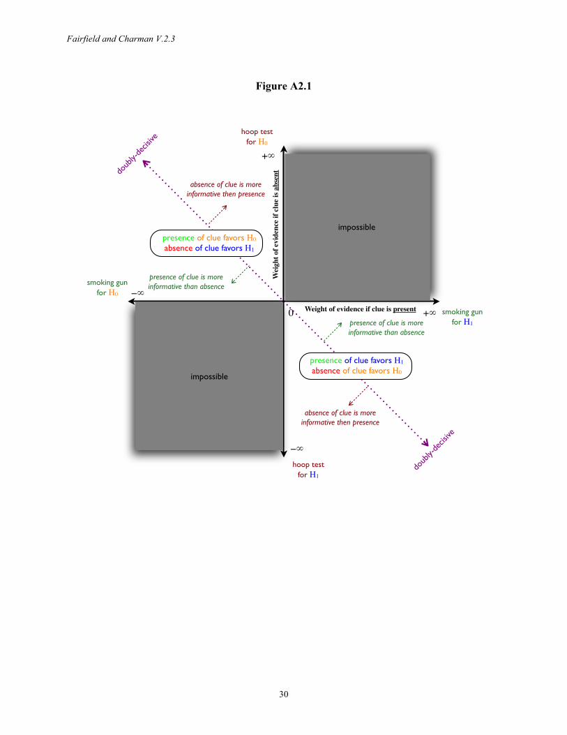
Fairfield and Charman V.2.3
30
Figure A2.1
Weight of evidence if clue is present
!"
+"0
!"
+"
impossible
impossible
presence of clue favors H1absence of clue favors H0
doub
ly-de
cisive
doub
ly-de
cisive
presence of clue is more informative than absence
absence of clue is more informative then presence
presence of clue favors H0absence of clue favors H1
smoking gunfor H1
smoking gunfor H0
hoop testfor H1
hoop testfor H0
absence of clue is more informative then presence
presence of clue is more informative than absence
Wei
ght o
f evi
denc
e if
clue
is a
bsen
t
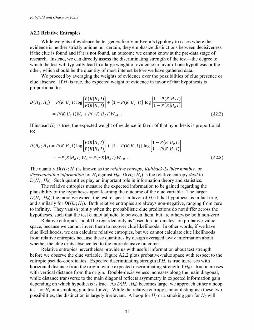
Fairfield and Charman V.2.3
31
A2.2 Relative Entropies
While weights of evidence better generalize Van Evera’s typology to cases where the evidence is neither strictly unique nor certain, they emphasize distinctions between decisiveness if the clue is found and if it is not found, an outcome we cannot know at the pre-data stage of research. Instead, we can directly assess the discriminating strength of the test—the degree to which the test will typically lead to a large weight of evidence in favor of one hypothesis or the other, which should be the quantity of most interest before we have gathered data.
We proceed by averaging the weights of evidence over the possibilities of clue presence or clue absence. If H1 is true, the expected weight of evidence in favor of that hypothesis is proportional to:
𝐷 𝐻1 ;𝐻o = 𝑃 𝐾 𝐻1 𝐼 log𝑃 𝐾 𝐻1 𝐼𝑃 𝐾 𝐻o 𝐼
+ 1 − 𝑃(𝐾|𝐻1 𝐼) log1 − 𝑃 𝐾 𝐻1 𝐼1 − 𝑃 𝐾 𝐻o 𝐼
= 𝑃 𝐾 𝐻1 𝐼 𝑊! + 𝑃 ~𝐾 𝐻1 𝐼 𝑊~! . (𝐴2.2) If instead H0 is true, the expected weight of evidence in favor of that hypothesis is proportional to:
𝐷 𝐻o ;𝐻1 = 𝑃 𝐾 𝐻o 𝐼 log𝑃 𝐾 𝐻o 𝐼𝑃 𝐾 𝐻1 𝐼
+ 1 − 𝑃(𝐾|𝐻o 𝐼) log1 − 𝑃 𝐾 𝐻o 𝐼1 − 𝑃 𝐾 𝐻1 𝐼
= −𝑃 𝐾 𝐻o 𝐼 𝑊! − 𝑃 ~𝐾 𝐻o 𝐼 𝑊~! . (𝐴2.3) The quantity D(H1 ; H0) is known as the relative entropy, Kullback-Leibler number, or discrimination information for H1 against H0. D(H0 ; H1) is the relative entropy dual to D(H1 ; H0). Such quantities play an important role in information theory and statistics.
The relative entropies measure the expected information to be gained regarding the plausibility of the hypotheses upon learning the outcome of the clue variable. The larger D(H1 ; H0), the more we expect the test to speak in favor of H1 if that hypothesis is in fact true, and similarly for D(H0 ; H1). Both relative entropies are always non-negative, ranging from zero to infinity. They vanish jointly when the probabilistic clue predictions do not differ across the hypotheses, such that the test cannot adjudicate between them, but are otherwise both non-zero.
Relative entropies should be regarded only as “pseudo-coordinates” on probative-value space, because we cannot invert them to recover clue likelihoods. In other words, if we have clue likelihoods, we can calculate relative entropies, but we cannot calculate clue likelihoods from relative entropies because these quantities by design averaged away information about whether the clue or its absence led to the more decisive outcome.
Relative entropies nevertheless provide us with useful information about test strength before we observe the clue variable. Figure A2.2 plots probative-value space with respect to the entropic pseudo-coordinates. Expected discriminating strength if H1 is true increases with horizontal distance from the origin, while expected discriminating strength if H0 is true increases with vertical distance from the origin. Double-decisiveness increases along the main diagonal, while distance transverse to the main diagonal reflects asymmetry in expected information gain depending on which hypothesis is true. As D(H1 ; H0) becomes large, we approach either a hoop test for H1 or a smoking gun test for H0. While the relative entropy cannot distinguish these two possibilities, the distinction is largely irrelevant. A hoop for H1 or a smoking gun for H0 will
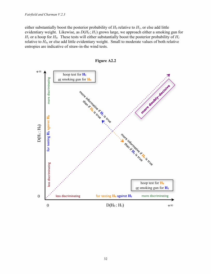
Fairfield and Charman V.2.3
32
either substantially boost the posterior probability of H0 relative to H1, or else add little evidentiary weight. Likewise, as D(H0 ; H1) grows large, we approach either a smoking gun for H1 or a hoop for H0. These tests will either substantially boost the posterior probability of H1 relative to H0, or else add little evidentiary weight. Small to moderate values of both relative entropies are indicative of straw-in-the wind tests.
Figure A2.2
D(H0 ; H1) +!0
more informative if H0 is true
than if H1 is true
more discriminating
+!
D(H
1 ; H
0)
0
more informative if H1 is true
than if H0 is true
less discriminating for testing H0 against H1
less
dis
crim
inat
ing
mor
e di
scri
min
atin
gfo
r te
stin
g H
1 ag
ains
t H
0
hoop test for H0 or smoking gun for H1
hoop test for H1 or smoking gun for H0
more
doubl
y-dec
isive
Fairfield and Charman V.2.3
33
A2.3 Test Strength as Expected Information Gain
At the pre-data stage, it makes sense not only to average over possible clue outcomes, but also to average over our prior uncertainty regarding which hypothesis is correct. In this way we can obtain the overall discrimination information, or expected information gain, from the test: 𝐷 = 𝑃 𝐻1 𝐼 𝐷 𝐻1 ;𝐻o + 𝑃 𝐻o 𝐼 𝐷 𝐻o ;𝐻1
= 𝑃 𝐻1 𝐼 𝐷 𝐻1 ;𝐻o + 1 − 𝑃 𝐻1 𝐼) 𝐷(𝐻o ;𝐻1) . (𝐴2.4)
The quantity D is the most natural pre-data measure of test strength, which tells us how loudly we expect the test to speak in favor of the best hypothesis. It ranges from zero to positive infinity. It is zero if and only if the clue probabilities under both hypotheses are the same, such that no learning can take place from the evidence. It is infinite if and only if one of the two relative entropies is infinite, meaning there must be at least one clue outcome that is impossible under one hypothesis yet possible under the other. D treats both hypotheses and both clue outcomes on equal footings, in that it is invariant under exchanging the roles of H0 and H1 and/or K and ~K. D effectively combines clue likelihoods and priors on the hypotheses into a single measure of the expected amount of information relevant to adjudicating between the hypotheses.
While no additional quantities beyond D are necessary for assessing test strength, a second, independent function is useful if we want to be able to invert back to the relative entropy pseudo-coordinates. A natural choice is some measure of the expected asymmetry of test decisiveness with respect to the two hypotheses—for example, the between-hypothesis component of the variance in the weight of evidence. The square root of this variance, ∆ 𝐻1 ;𝐻o = 𝑃(𝐻1 𝐼 𝑃(𝐻o|𝐼) × 𝐷 𝐻1 ;𝐻o − 𝐷(𝐻o ;𝐻1) , (𝐴2.5) is convenient for this purpose.
Figure A2.3 plots the asymmetry Δ versus the information gain D. Weak tests fall close to the origin; test strength increases with the value of D. Smaller values of Δ indicate greater symmetry, or more doubly-decisive tests. Strong but singly-decisive tests (hoop or smoking-gun) occur for large values of D and large values of Δ; the sign of Δ indicates the hypothesis under which the test is expected to be more decisive.
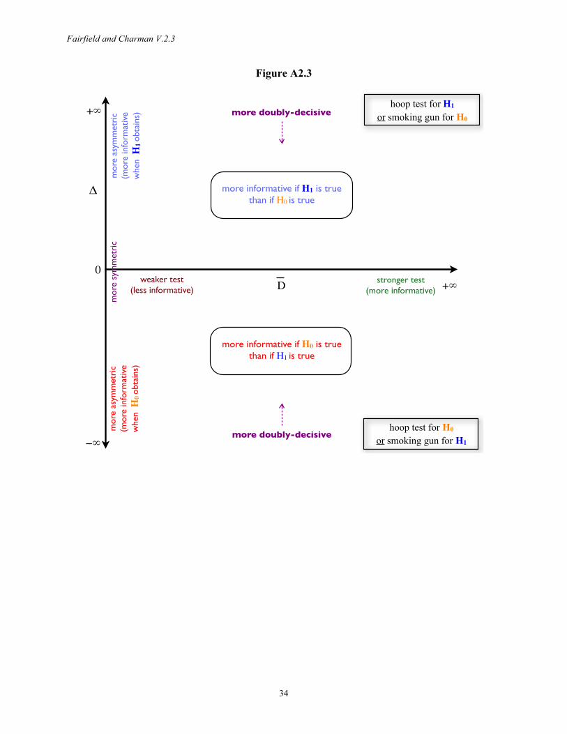
Fairfield and Charman V.2.3
34
Figure A2.3
stronger test(more informative)
+!
0weaker test
(less informative)
more informative if H1 is truethan if H0 is true
D
"
#!
+!
more informative if H0 is truethan if H1 is true
mor
e sy
mm
etri
cm
ore
asym
met
ric
(mor
e in
form
ativ
e w
hen
H0 ob
tain
s)
mor
e as
ymm
etri
c(m
ore
info
rmat
ive
whe
n H
1 ob
tain
s) more doubly-decisive
more doubly-decisive
hoop test for H1 or smoking gun for H0
hoop test for H0 or smoking gun for H1
Fairfield and Charman V.2.3
35
A3. Applying Formal Bayesian Analysis to Qualitative Case Research: An Empirical Example
To illustrate how Bayesian logic underpins qualitative research, we provide an application to Fairfield’s (2015) work on tax policy change in Latin America. Fairfield (2013) elaborated a methodological appendix that we believe is the first published account that explicitly uses process-tracing tests to elucidate causal inferences in the author’s case narratives. In the following exercise, which is also the first of its kind, we revise that appendix by replacing the language of process-tracing tests with direct applications of Bayes’ theorem. While we advocate a Bayesian approach to inference over process-tracing tests, which remain close in spirit to a frequentist approach, we wish to stress from the outset the difficulty of quantifying probabilities in the complex world of social science.
In Private Wealth and Public Revenue in Latin America, Fairfield (2015) analyzes how and when unequal democracies can tax economic elites. Fairfield explains the scope and fate of tax policy proposals by analyzing business’s instrumental (political) power and structural (investment) power. Instrumental power entails deliberate political actions like lobbying. Structural power arises from the profit-maximizing behavior of firms and investors; if policymakers anticipate that a reform will provoke disinvestment or capital flight, they may rule it out to protect growth and employment. When business actors have strong power of either type, their interests shape policy decisions. However, strategies for mobilizing public support or tempering elite opposition can facilitate incremental reforms that might not otherwise be feasible. One such strategy—a vertical equity appeal—aims to mobilize public support by emphasizing a tax increases’ congruence with the widely-accepted principle that those who earn more or own more assets should bear a larger share of the tax burden.
Fairfield’s (2013) article on tax reform strategies includes the case of a 2005 Chilean reform that eliminated a longstanding tax benefit (article “57 bis”) for owners of new-issue stocks who belonged to the richest 0.5%. During the presidential campaign, Chile’s Catholic bishops forcefully denounced the country’s extreme levels of inequality, thereby raising the salience of this issue. Right-coalition candidate Lavín responded by blaming Chile’s persistent inequality on the governing left coalition and accusing incumbent president Lagos of failing to deliver his promise of growth with equity. Lagos seized the opportunity to eliminate article 57 bis by linking the reform to the issue of inequality and thereby mobilizing public support with the following equity appeal: “The famous Article 57 bis is still in force and signifies a tremendous source of inequality. …Instead of just talking, why don’t we agree to eliminate 57 bis in less than 24 hours?”23 The right, which held a majority in the senate, accepted the challenge and voted in favor of eliminating the tax benefit, deviating from its prior position on this policy as well as the preferences of its core constituency—business owners and upper-income individuals. Before proceeding, readers may wish to read Fairfield’s (2013) original case narrative (Appendix 4).
This case was chosen for explicit consideration of process-tracing tests for both substantive and practical reasons. Substantively, the 2005 reform was an emblematic case of equity-enhancing tax reform in Chile that illustrates both the importance of strategies that mobilize public support and the limitations to how much revenue they can raise in contexts of strong business power. Practically, this is a clear-cut case in which a relatively small number of key pieces of evidence establish the causal importance of the reform strategy. As the complexity of
23Lagos, quoted in “Lagos reta a Alianza a derogar exención tributaria en 24 horas,” El Mercurio, May 10, 2005.
Fairfield and Charman V.2.3
36
the case and the quantity of evidence the analyst draws on to make inferences increase, explicit elaboration of either process tracing tests or the formal Bayesian reasoning we employ here may become infeasible.
A3.1 Specifying Hypotheses
Fairfield (2013, 2015) argues that Lagos’ equity appeal, which took place in an unusual context of strong electoral competition from the right coalition on the issue of inequality, was critical for eliminating 57 bis. The postulated causal mechanism is that in this unusual context, the equity appeal created concern within the right coalition that rejecting the tax initiative would damage its candidate’s electoral prospects.
HEA: Lagos’ equity appeal, in the context of a presidential campaign where inequality had assumed high issue-salience, drove the right to accept the 2005 reform in order to avoid electoral costs. ~HEA: The right would have accepted the 2005 reform anyway—without the equity appeal in the context of a major electoral campaign where inequality had assumed high issue-salience. In other words, those factors did not have an important causal effect on the fate of the reform initiative.
Whereas frequentists usually consider a single null hypothesis and its negation, applying Bayes’ theorem requires elaborating a complete set of mutually exclusive hypotheses. We need to explicitly state the alternatives before we can reason meaningfully about the likelihood of observing the evidence if the author’s hypothesis does not hold (see Section 3.7). To that end, we decompose ~HEA into three rival alternative hypotheses:
HI: The right accepted the reform because Chile’s institutionalized party system and stable rules of the game motivate cross-partisan cooperation in congress and consensual politics (drawing on Flores-Macías 2010). These institutions lengthen time horizons and encourage parties to moderate their policy stances in anticipation of future rounds of negotiation on other issues. HP: The right accepted the reform because the preferences of its core constituency—business and upper-income individuals—had changed. Over time, the number of individuals benefitting from 57 bis had declined as owners sold their new-issue stocks and acquired other assets,24 so the right’s core constituency no longer had a material interest in defending the tax benefit. HMV: The right accepted the 2005 reform in accord with a simple median voter model of redistributive politics, where electoral competition drives politicians to converge on policies that promote the median voters’ material interests (e.g. Meltzer and Richard 1981). In other words, Lagos’ equity appeal and the specific
24A reform in the 1990s had precluded new entrants but grandfathered in existing beneficiaries (Fairfield 2015, Chapter 4).
Fairfield and Charman V.2.3
37
context in which it took place were irrelevant for obtaining right votes in support of eliminating 57 bis.
It is important to note that we are assuming as part of our background information that
these alternative hypotheses are mutually exclusive and exhaustive—in other words, only one of the mechanisms corresponding to the four different hypotheses may operate. Otherwise we cannot maintain that ~HEA = HI + HP + HMV. In the real world, one could imagine that the equity appeal might work to create consensus between the right and the left, but that logic corresponds to a more complex causal hypothesis that blends elements of both HEA and HI. Similarly, it might be the case that changing business preferences in conjunction with the equity appeal motivated the right to accept the reform, such that a combination of both HEA and HP was critical to the outcome. Allowing for causal complexity in which multiple mechanisms operate at the same time, to varying degrees or in interaction, would require elaborating additional, more complicated mutually exclusive hypotheses, which can be challenging if we wish to be precise enough to apply formal Bayesian analysis (Section 3.2). A3.2 Assigning Priors
We consider three different prior distributions for the four hypotheses. For the first prior, we employ the indifference principle and set equal probabilities of 25% on each hypothesis, since from a position of maximal ignorance I0, we have no reason to privilege any one of the four explanations. This approach aims to approximate objective Bayesianism (Section 3.3); however, it ignores the background information we bring to the analysis for lack of any feasible way to systematically build up from I0 to incorporate our full background information I.
The second prior distribution aims to take into consideration the large body of literature questioning the logic underlying simple median-voter models. Authors have identified numerous assumptions in these models that do not hold up against empirical evidence—not only for developed countries like the US (Hacker and Pierson 2010), but also for developing countries (Kaufman 2009). For the case of Chile, Luna (2014) analyzes in detail how right parties have successfully defended the economic interests of their core upper-income constituency while still managing to win broad support among low-income voters who would stand to benefit from redistribution. Accordingly, we place a low subjective prior probability on HMV of 0.001% and equal probabilities on HEA, HI, and HP of 33.3%. These assignments correspond to a prior log-odds ratio of 45 dB against HMV relative to each of the other hypotheses. Using our sound analogy (Section 3.6), we could say that HMV is “sleeping” in the background, and it would take roughly 45 dB to “wake it up” (Table 1 below). It is worth emphasizing that from a more objective Bayesian perspective, instead of relying on our intuition to penalize HMV we should begin with our indifference priors and systematically incorporate every piece of evidence we have that bears on the hypotheses. That approach is clearly infeasible in practical terms. For example, we would need to assess every piece of qualitative and quantitative evidence that Luna (2014) provides in his extensive analysis, not to mention all other works in the large body of literature on median voter theories and redistribution.
The third prior distribution, which is also subjective in nature, draws on comments received from a reviewer on a draft of Fairfield’s 2013 article. The reviewer expressed significant skepticism that a presidential appeal could affect reform outcomes, citing examples from US
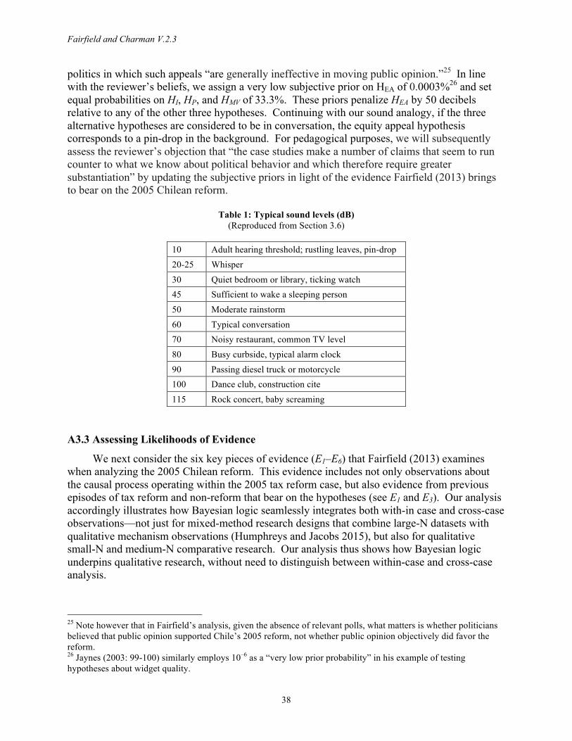
Fairfield and Charman V.2.3
38
politics in which such appeals “are generally ineffective in moving public opinion.”25 In line with the reviewer’s beliefs, we assign a very low subjective prior on HEA of 0.0003%26 and set equal probabilities on HI, HP, and HMV of 33.3%. These priors penalize HEA by 50 decibels relative to any of the other three hypotheses. Continuing with our sound analogy, if the three alternative hypotheses are considered to be in conversation, the equity appeal hypothesis corresponds to a pin-drop in the background. For pedagogical purposes, we will subsequently assess the reviewer’s objection that “the case studies make a number of claims that seem to run counter to what we know about political behavior and which therefore require greater substantiation” by updating the subjective priors in light of the evidence Fairfield (2013) brings to bear on the 2005 Chilean reform.
Table 1: Typical sound levels (dB) (Reproduced from Section 3.6)
10 Adult hearing threshold; rustling leaves, pin-drop 20-25 Whisper 30 Quiet bedroom or library, ticking watch 45 Sufficient to wake a sleeping person 50 Moderate rainstorm 60 Typical conversation 70 Noisy restaurant, common TV level 80 Busy curbside, typical alarm clock 90 Passing diesel truck or motorcycle 100 Dance club, construction cite 115 Rock concert, baby screaming
A3.3 Assessing Likelihoods of Evidence
We next consider the six key pieces of evidence (E1–E6) that Fairfield (2013) examines when analyzing the 2005 Chilean reform. This evidence includes not only observations about the causal process operating within the 2005 tax reform case, but also evidence from previous episodes of tax reform and non-reform that bear on the hypotheses (see E1 and E3). Our analysis accordingly illustrates how Bayesian logic seamlessly integrates both with-in case and cross-case observations—not just for mixed-method research designs that combine large-N datasets with qualitative mechanism observations (Humphreys and Jacobs 2015), but also for qualitative small-N and medium-N comparative research. Our analysis thus shows how Bayesian logic underpins qualitative research, without need to distinguish between within-case and cross-case analysis.
25 Note however that in Fairfield’s analysis, given the absence of relevant polls, what matters is whether politicians believed that public opinion supported Chile’s 2005 reform, not whether public opinion objectively did favor the reform. 26 Jaynes (2003: 99-100) similarly employs 10–6 as a “very low prior probability” in his example of testing hypotheses about widget quality.
Fairfield and Charman V.2.3
39
To apply Bayes’ theorem, we need to assign conditional probabilities, or likelihoods, denoted P(Ex |Hj Eprev I) to each piece of evidence Ex. In other words, we must quantify how likely a given piece of evidence Ex is to be found under each of the four hypotheses, {Hj, j = EA, I, P, MV}, conditional on the pieces of evidence that we have previously incorporated into our analysis, Eprev, and on our background information, I.
Assigning numerical values, or even rank ordering these probabilities, is challenging. Ideally, one should reason out each probability in the problem and then calculate likelihood ratios P(Ex |Hj Eprev I) ⁄ P(Ex |Hk Eprev I) to assess how much a given piece of evidence discriminates between a pair of hypotheses. In practice, however, it is very difficult to assess what absolute value a likelihood should assume when conditioning a piece of evidence on a hypothesis that simply does not fit. We know the likelihood of viewing the evidence should be very low, but our intuition gives us little traction for discerning whether that likelihood should be lower or higher than the probability of viewing some other piece of evidence that is extremely unlikely under another hypothesis. Our brains simply are not accustomed to making judgments on these scales—it is very difficult to assess differences between probabilities that are extremely small. To circumvent this problem, we opted for the following approach.
First, we set values for the likelihood of each piece of evidence under the most compatible hypothesis—this task entails handling probabilities in a range for which we feel capable of making reasonable assignments. Second, we used our intuition to assess how large the log-likelihood ratio should be for each piece of evidence relative to the rival hypotheses. This approach is natural since only the relative probabilities of observing the evidence under different hypotheses matter for assessing which explanation fits best, and because it is easier for our brains to perceive and interpret differences on a logarithmic scale (Section 3.6). For evidence that strongly discriminates between two hypotheses, we assign a likelihood ratio of 103, making the weight of evidence (ten times the log of the likelihood ratio) 30 decibels. Employing the analogy of inference as a dialog with the data, 30 decibels in acoustic terms roughly corresponds to the difference between a quiet bedroom and an ordinary conversation—in other words, the data are “talking clearly.” Very low probabilities were then determined by the baseline probability of the evidence in question under the most compatible hypothesis and the likelihood ratio relative to the rival hypotheses. We adjusted low probabilities as necessary when a clear argument could be made that a given likelihood should be higher or lower than another likelihood in the exercise. Our lowest probability assignments, for evidence that we view as exceedingly unlikely under a given hypothesis, are on the order of 10–5: extremely improbable, but a healthy order of magnitude higher than being struck by lightening over a lifetime (10–6) and several orders of magnitude larger than other relevant improbable perils such as experiencing a plane crash on a major airline (10–7) or winning a major lottery (10–8).
Readers may nevertheless object that our lowest probabilities are too small. In response, we emphasize that we are using a logarithmic scale because humans have evolved to deal with probabilities that vary over orders of magnitude. A logarithmic scale is actually better suited to human perception than a more familiar linear scale, once we become accustomed to working in decibels. Moreover, our two-step procedure for assigning improbable likelihoods minimizes—although hardly removes—the arbitrariness of quantifying inherently qualitative data. Readers should find the likelihoods we assign under the hypothesis that fits best (ranging from 3%–60%) to be reasonable. And the analogy to sound levels helps make assessments of likelihood ratios as consistent and intuitive as possible. Together, these two factors uniquely determine likelihoods under rival hypotheses that would otherwise be extremely difficult to reliably quantify. In our
Fairfield and Charman V.2.3
40
experience, the formalization exercise would have been intractable and fraught with inconsistencies had we not devised the procedure outlined above. A final critical point is that the primary objective in social science should be comparing hypotheses, rather than calculating posteriors, in which case only the likelihood ratios matter—not the absolute value of the probabilities. For readers whose skepticism persists, we assess how our conclusions would change if we were to compress our likelihood ratios—increasing our lowest probabilities by a factor of 50—in the last section of this appendix.
Assessing probabilities conditional on previously-incorporated evidence presents additional challenges, as discussed in Section 3.5. This task entails asking whether Ex and Eprev have any logical dependence under the assumption that Hj is true: what do we learn about the likelihood of Ex from observing Eprev? Beyond what Hj tells us, if we also know Eprev, are we any more or less likely to observe Ex, and by how much? Answering these questions can be very difficult. Evidence can be connected in arbitrarily complex ways that make tracing through possible logical and/or causal connections a complicated task. It could even be the case that two pieces of evidence Ex and Ey are dependent in multiple ways, some of which might lead us to raise P(Ex |Hj Ey) above P(Ex |Hj), whereas others might lead us to lower P(Ex |Hj Ey). When the data are qualitative, quantifying potentially competing effects from different linkages may be practically impossible. Even in the relatively simple example we examine here, we managed to explicitly condition on only those pieces of evidence that are most clearly dependent under a given hypothesis.
The background information, upon which all probability assignments are also conditioned, draws on extensive fieldwork in Chile that included 216 interviews, research in news and congressional archives, and observation of congressional proceedings, conferences, and public events relevant to tax policy. The background information includes knowledge about effort expended to uncover relevant evidence, persistence in seeking to obtain interviews, relative ease or difficulty of reaching particular types of informants, skill at establishing rapport with and degree of trust in informants, first-hand knowledge about Chilean politics, and a wide range of contextual clues that inform interpretation of interviews and other evidence. We also take the particular set of informants interviewed as part of the background information, to avoid reasoning about the probability of reaching a specific individual or type of informant when assessing likelihoods. For example, E2 includes a statement made by former president Lagos; we condition the likelihood of E2 on the background information that Fairfield was able to interview Lagos on multiple occasions. Otherwise, we would have to lower the likelihood of E2 under each hypothesis. We explicitly discuss specific elements of the background information that inform likelihood assignments as needed. However, much of the background information inevitably remains implicit; in practice it would be impossible to fully enumerate.
It is also important to note that although E1–E6 mention very specific pieces of evidence obtained during fieldwork, the conditional probabilities we assign below correspond to any informationally-equivalent piece of evidence that might have arisen. For example, P(E6|HEA Eprev I) refers to the likelihood of a particular right-party deputy interviewed on December 23, 2005 sharing the exact comments reported, or to any other essentially equivalent story shared by a similar informant from that party, using slightly different language, on a different day, and so forth. This point may seem like a technicality, but the probability of observing the exact piece of evidence E6 would otherwise be vanishingly small given the myriad contingencies that ultimately produced that specific conversation. Moreover, irrelevant details associated with a narrowly-defined piece of evidence would be common under each alternative
Fairfield and Charman V.2.3
41
hypothesis—they would simply lower the conditional probability of the evidence under every hypothesis, such that their effect would cancel out of the likelihood ratios.
In general, defining the equivalence class entails optimizing a tradeoff between generality and specificity. If the equivalence class is too broad and vague, we may risk circularity by essentially asserting that “the evidence is that there was evidence in favor of the hypothesis,” and there will be little basis for assessing likelihoods. If the equivalence class becomes too narrow and specific, with too many irrelevant details, the likelihoods will become vanishingly small and hence difficult to assess, since our brains are not well adapted for reasoning about small probabilities. The set of hypotheses under consideration will also guide decisions about how narrowly or broadly to define the equivalence class for the sake of effectively discriminating among the explanations.
In most cases below, the equivalence class is implicitly defined by the details that are omitted in stating the evidence. For example, if a quote is attributed to an informant of a particular type, a similar statement from an alternative informant of that same type would be assigned the same probability.
We now proceed to assess likelihoods for the six different pieces of evidence given the alternative hypotheses. In assigning each probability, we draw on the considerations discussed above, including background information and logical dependence or independence of evidence. We also pay close attention to potential instrumental incentives and/or unmotivated biases that could affect a source’s inclination to make particular statements and/or disposition to reveal or conceal information.
E1 = The governing center-left coalition discussed eliminating 57 bis in multiple prior tax reforms (1990, 1995, 1998, 2001) (E1a). However, governing-coalition informants explained that the initiative was ultimately ruled out as infeasible on every such occasion due to resistance from the right (E1b). (E1a sources: Diario de Sesiones del Senado, Legislatura 331, Sesión 14, July 6, 1995: 37, and 338, Sesión 13, July 7, 1998: 64; interviews: Aninat, Montes, and all E1b interviews. E1b sources (interviews): Bitar, Executive Advisor A, Eyzaguirre, Ffrench-Davis, Finance Ministry-A, -B, -H, Jorratt, Marcel, Marfán)
We have endeavored to describe E1 in terms that convey an appropriate and manageable
equivalence class. What matters most for discriminating among our alternative hypotheses is the existence of multiple prior discussions about eliminating the tax benefit, not the details regarding how many times it was considered or in which years. Had we considered these details as central to the definition of E1, the likelihoods would become orders of magnitude smaller, and much more difficult to assess—the chances that discussion would take place in each of these particular years under any of the hypotheses is very, very low. Even if we take as part of the background information that tax reforms were enacted in these years, discussions of 57 bis could easily have occurred in some but not all of these years, or in other years when additional reforms were proposed. We include these details parenthetically, along with several of the sources of the information, to illustrate the concrete specifics of the data uncovered.27
Notice also that for convenience, we have taken E1 to be the conjunction of two pieces of information E1a and E1b. We could assess E1a and E1b separately as distinct pieces of evidence;
27Case narratives also include extensive details that go beyond the relevant equivalence class; this allows readers to assess alternative hypotheses the author knows to be patently inconsistent and hence does not explicitly consider.
Fairfield and Charman V.2.3
42
we could even disaggregate further so that each of the sources noted above contributes one or more pieces of evidence to be considered separately. However, there would be few analytical gains. When we are dealing with qualitative data, we need to operate at a level that facilitates reasoning, rather than trying to build up systematically from extremely specific bits of evidence. If we disaggregate too finely and if we make too many analytical steps explicit, we will become lost in minutia. The mathematics of Bayesian analysis allows us to aggregate or disaggregate data at whatever level is convenient. P(E1|HEA I) = 20% This evidence is consistent with the hypothesis that Lagos’ high-profile equity appeal in the unusual context of electoral competition from the right on the issue of inequality explains the right’s acceptance of the 2005 reform, since some new factor that was not present in previous years must have changed the right’s behavior. The probability of observing E1 will depend on how likely we think it is under the equity-appeal hypothesis that: 1) center-left governments would consider eliminating 57 bis on multiple prior occasions, 2) evidence of such discussions would be uncovered, given that they may or may not have taken place publicly, 3) the right would have resisted the initiative on all such occasions, and 4) governing-coalition informants would attribute their decision not to push forward with the initiative to resistance from the right. Regarding the first proposition, we take as background information that center-left governments were interested in raising revenue and eliminating tax privileges for the wealthy; however, eliminating 57 bis may not have been discussed at all if other issues had higher priority on the reform agenda. In contrast, we view propositions 2), 3) and 4) as highly probable. Regarding 2), we judge the probability of discovering evidence if prior initiatives were discussed to be high, drawing on the (logically prior) background information that Fairfield obtained extensive access to finance ministry informants who shared ample information about policy deliberations that was not part of the public record. For proposition 3), we view the probability of right resistance as very high given background information from prior research (Luna 2014) and from Fairfield’s research on other tax reforms in Chile that the right generally opposed increasing taxes and eliminating tax benefits on principle. Strictly speaking, by treating this information as background, it should also inform our priors on the hypotheses. Specifically, this information would lower the prior probability on HMV (and possibly HI as well). However, we will nevertheless consider priors that do not penalize HMV relative to other hypotheses for the sake of being conservative, and for the sake of highlighting the impact of the six pieces of evidence from the case study. Regarding proposition 4), given that the right held a majority in the senate during this period, we see no reason under HEA that center-left informants would not identify right resistance as a major impediment to reform. Ultimately, we somewhat arbitrarily assign P(E1|HEA) a value of 20%, in light of the possibility that any number of other progressive reform initiatives could have been prioritized in the past. In reality, this probability may be overestimated; however, recall that for the purpose of comparing hypotheses, only the relative likelihoods under the four hypotheses will matter. P(E1|HI I) = .02% If stable institutions produced consensus on eliminating 57 bis in 2005, they should have produced consensus on this initiative in previous years as well, since our background information includes the fact that institutions did not change during the intervening time period. If
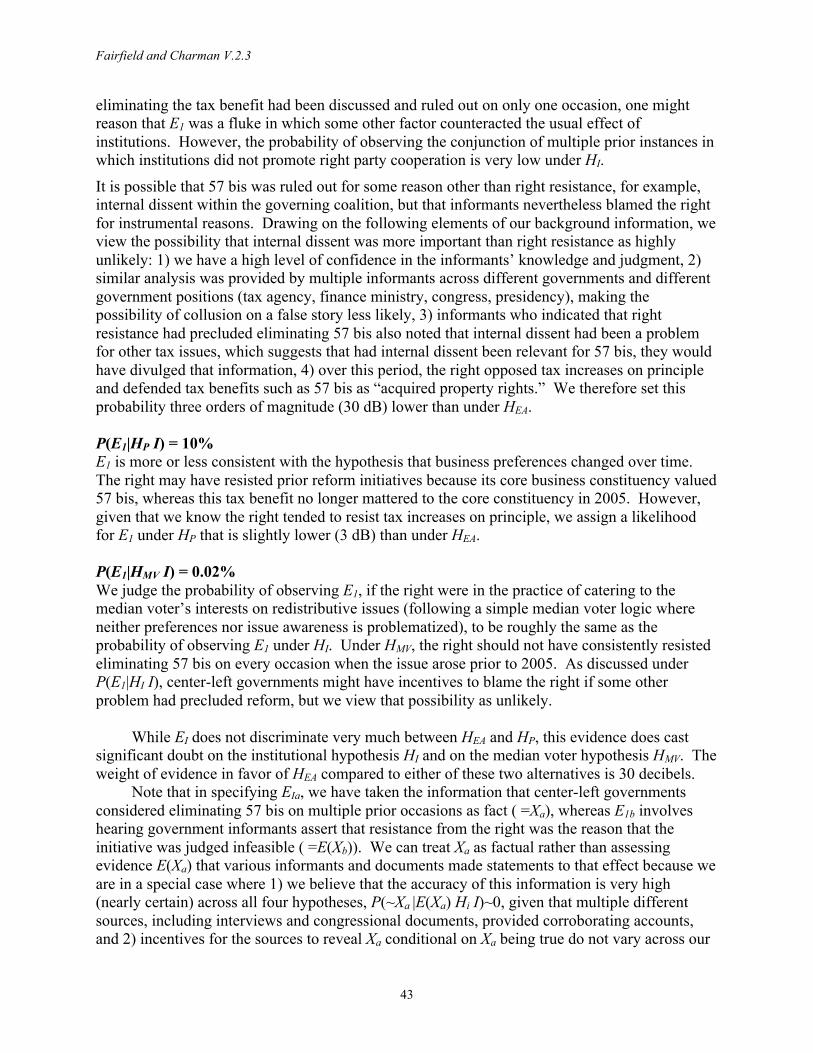
Fairfield and Charman V.2.3
43
eliminating the tax benefit had been discussed and ruled out on only one occasion, one might reason that E1 was a fluke in which some other factor counteracted the usual effect of institutions. However, the probability of observing the conjunction of multiple prior instances in which institutions did not promote right party cooperation is very low under HI.
It is possible that 57 bis was ruled out for some reason other than right resistance, for example, internal dissent within the governing coalition, but that informants nevertheless blamed the right for instrumental reasons. Drawing on the following elements of our background information, we view the possibility that internal dissent was more important than right resistance as highly unlikely: 1) we have a high level of confidence in the informants’ knowledge and judgment, 2) similar analysis was provided by multiple informants across different governments and different government positions (tax agency, finance ministry, congress, presidency), making the possibility of collusion on a false story less likely, 3) informants who indicated that right resistance had precluded eliminating 57 bis also noted that internal dissent had been a problem for other tax issues, which suggests that had internal dissent been relevant for 57 bis, they would have divulged that information, 4) over this period, the right opposed tax increases on principle and defended tax benefits such as 57 bis as “acquired property rights.” We therefore set this probability three orders of magnitude (30 dB) lower than under HEA. P(E1|HP I) = 10% E1 is more or less consistent with the hypothesis that business preferences changed over time. The right may have resisted prior reform initiatives because its core business constituency valued 57 bis, whereas this tax benefit no longer mattered to the core constituency in 2005. However, given that we know the right tended to resist tax increases on principle, we assign a likelihood for E1 under HP that is slightly lower (3 dB) than under HEA. P(E1|HMV I) = 0.02% We judge the probability of observing E1, if the right were in the practice of catering to the median voter’s interests on redistributive issues (following a simple median voter logic where neither preferences nor issue awareness is problematized), to be roughly the same as the probability of observing E1 under HI. Under HMV, the right should not have consistently resisted eliminating 57 bis on every occasion when the issue arose prior to 2005. As discussed under P(E1|HI I), center-left governments might have incentives to blame the right if some other problem had precluded reform, but we view that possibility as unlikely.
While EI does not discriminate very much between HEA and HP, this evidence does cast significant doubt on the institutional hypothesis HI and on the median voter hypothesis HMV. The weight of evidence in favor of HEA compared to either of these two alternatives is 30 decibels.
Note that in specifying EIa, we have taken the information that center-left governments considered eliminating 57 bis on multiple prior occasions as fact ( =Xa), whereas E1b involves hearing government informants assert that resistance from the right was the reason that the initiative was judged infeasible ( =E(Xb)). We can treat Xa as factual rather than assessing evidence E(Xa) that various informants and documents made statements to that effect because we are in a special case where 1) we believe that the accuracy of this information is very high (nearly certain) across all four hypotheses, P(~Xa |E(Xa) Hi I)~0, given that multiple different sources, including interviews and congressional documents, provided corroborating accounts, and 2) incentives for the sources to reveal Xa conditional on Xa being true do not vary across our
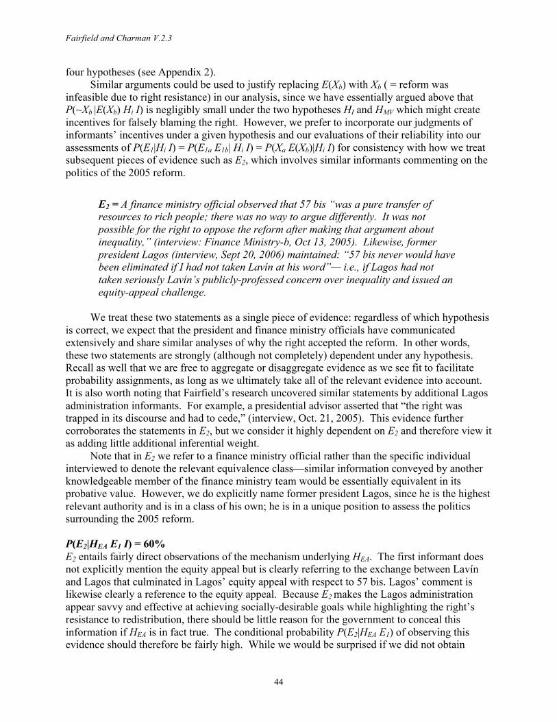
Fairfield and Charman V.2.3
44
four hypotheses (see Appendix 2). Similar arguments could be used to justify replacing E(Xb) with Xb ( = reform was
infeasible due to right resistance) in our analysis, since we have essentially argued above that P(~Xb |E(Xb) Hi I) is negligibly small under the two hypotheses HI and HMV which might create incentives for falsely blaming the right. However, we prefer to incorporate our judgments of informants’ incentives under a given hypothesis and our evaluations of their reliability into our assessments of P(E1|Hi I) = P(E1a E1b| Hi I) = P(Xa E(Xb)|Hi I) for consistency with how we treat subsequent pieces of evidence such as E2, which involves similar informants commenting on the politics of the 2005 reform.
E2 = A finance ministry official observed that 57 bis “was a pure transfer of resources to rich people; there was no way to argue differently. It was not possible for the right to oppose the reform after making that argument about inequality,” (interview: Finance Ministry-b, Oct 13, 2005). Likewise, former president Lagos (interview, Sept 20, 2006) maintained: “57 bis never would have been eliminated if I had not taken Lavín at his word”— i.e., if Lagos had not taken seriously Lavín’s publicly-professed concern over inequality and issued an equity-appeal challenge.
We treat these two statements as a single piece of evidence: regardless of which hypothesis
is correct, we expect that the president and finance ministry officials have communicated extensively and share similar analyses of why the right accepted the reform. In other words, these two statements are strongly (although not completely) dependent under any hypothesis. Recall as well that we are free to aggregate or disaggregate evidence as we see fit to facilitate probability assignments, as long as we ultimately take all of the relevant evidence into account. It is also worth noting that Fairfield’s research uncovered similar statements by additional Lagos administration informants. For example, a presidential advisor asserted that “the right was trapped in its discourse and had to cede,” (interview, Oct. 21, 2005). This evidence further corroborates the statements in E2, but we consider it highly dependent on E2 and therefore view it as adding little additional inferential weight.
Note that in E2 we refer to a finance ministry official rather than the specific individual interviewed to denote the relevant equivalence class—similar information conveyed by another knowledgeable member of the finance ministry team would be essentially equivalent in its probative value. However, we do explicitly name former president Lagos, since he is the highest relevant authority and is in a class of his own; he is in a unique position to assess the politics surrounding the 2005 reform. P(E2|HEA E1 I) = 60% E2 entails fairly direct observations of the mechanism underlying HEA. The first informant does not explicitly mention the equity appeal but is clearly referring to the exchange between Lavín and Lagos that culminated in Lagos’ equity appeal with respect to 57 bis. Lagos’ comment is likewise clearly a reference to the equity appeal. Because E2 makes the Lagos administration appear savvy and effective at achieving socially-desirable goals while highlighting the right’s resistance to redistribution, there should be little reason for the government to conceal this information if HEA is in fact true. The conditional probability P(E2|HEA E1) of observing this evidence should therefore be fairly high. While we would be surprised if we did not obtain
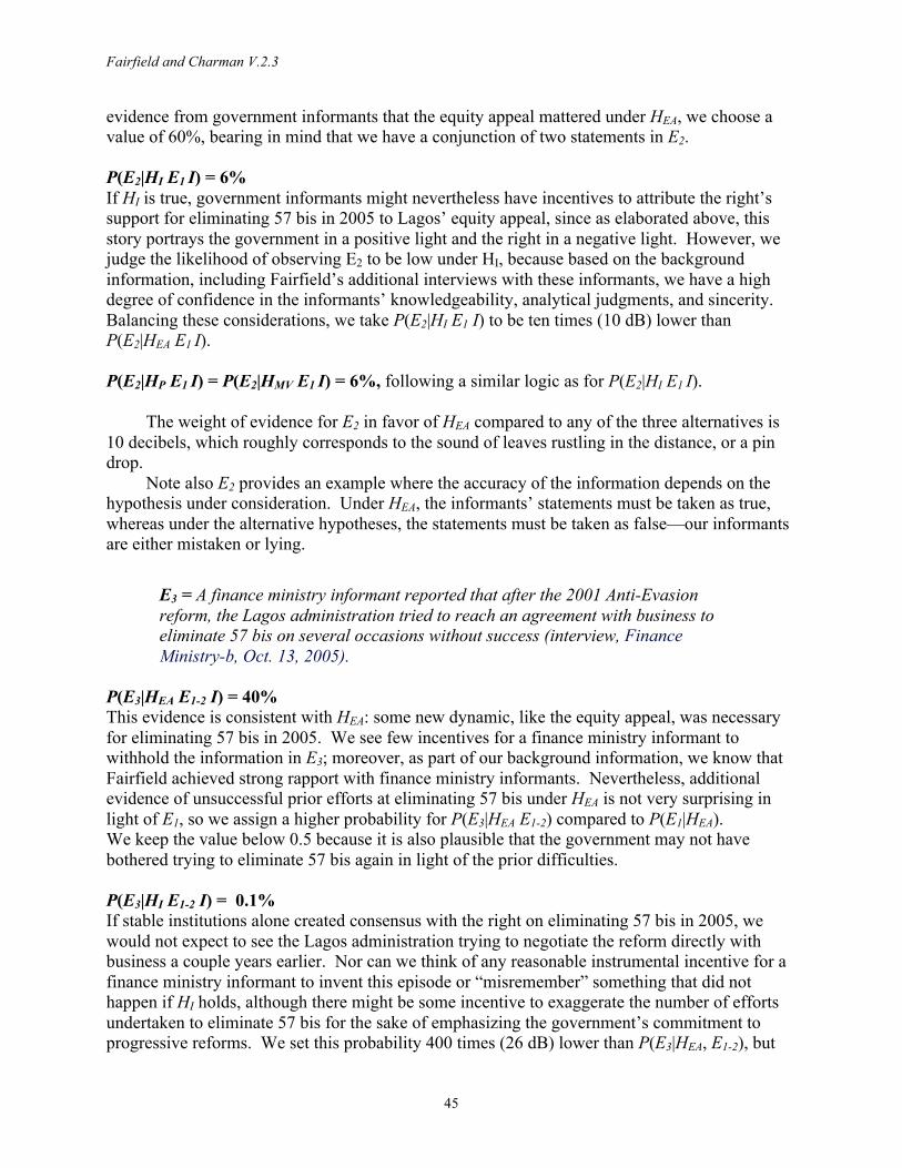
Fairfield and Charman V.2.3
45
evidence from government informants that the equity appeal mattered under HEA, we choose a value of 60%, bearing in mind that we have a conjunction of two statements in E2. P(E2|HI E1 I) = 6% If HI is true, government informants might nevertheless have incentives to attribute the right’s support for eliminating 57 bis in 2005 to Lagos’ equity appeal, since as elaborated above, this story portrays the government in a positive light and the right in a negative light. However, we judge the likelihood of observing E2 to be low under HI, because based on the background information, including Fairfield’s additional interviews with these informants, we have a high degree of confidence in the informants’ knowledgeability, analytical judgments, and sincerity. Balancing these considerations, we take P(E2|HI E1 I) to be ten times (10 dB) lower than P(E2|HEA E1 I). P(E2|HP E1 I) = P(E2|HMV E1 I) = 6%, following a similar logic as for P(E2|HI E1 I).
The weight of evidence for E2 in favor of HEA compared to any of the three alternatives is 10 decibels, which roughly corresponds to the sound of leaves rustling in the distance, or a pin drop.
Note also E2 provides an example where the accuracy of the information depends on the hypothesis under consideration. Under HEA, the informants’ statements must be taken as true, whereas under the alternative hypotheses, the statements must be taken as false—our informants are either mistaken or lying.
E3 = A finance ministry informant reported that after the 2001 Anti-Evasion reform, the Lagos administration tried to reach an agreement with business to eliminate 57 bis on several occasions without success (interview, Finance Ministry-b, Oct. 13, 2005).
P(E3|HEA E1-2 I) = 40% This evidence is consistent with HEA: some new dynamic, like the equity appeal, was necessary for eliminating 57 bis in 2005. We see few incentives for a finance ministry informant to withhold the information in E3; moreover, as part of our background information, we know that Fairfield achieved strong rapport with finance ministry informants. Nevertheless, additional evidence of unsuccessful prior efforts at eliminating 57 bis under HEA is not very surprising in light of E1, so we assign a higher probability for P(E3|HEA E1-2) compared to P(E1|HEA). We keep the value below 0.5 because it is also plausible that the government may not have bothered trying to eliminate 57 bis again in light of the prior difficulties. P(E3|HI E1-2 I) = 0.1% If stable institutions alone created consensus with the right on eliminating 57 bis in 2005, we would not expect to see the Lagos administration trying to negotiate the reform directly with business a couple years earlier. Nor can we think of any reasonable instrumental incentive for a finance ministry informant to invent this episode or “misremember” something that did not happen if HI holds, although there might be some incentive to exaggerate the number of efforts undertaken to eliminate 57 bis for the sake of emphasizing the government’s commitment to progressive reforms. We set this probability 400 times (26 dB) lower than P(E3|HEA, E1-2), but
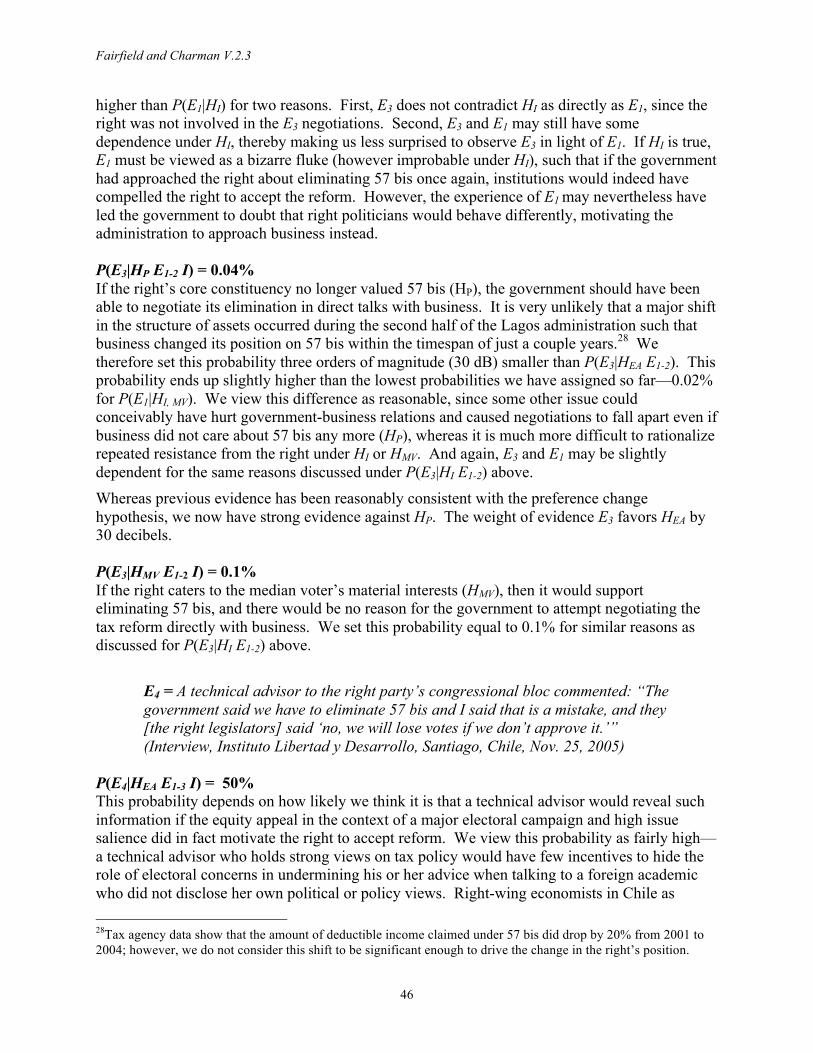
Fairfield and Charman V.2.3
46
higher than P(E1|HI) for two reasons. First, E3 does not contradict HI as directly as E1, since the right was not involved in the E3 negotiations. Second, E3 and E1 may still have some dependence under HI, thereby making us less surprised to observe E3 in light of E1. If HI is true, E1 must be viewed as a bizarre fluke (however improbable under HI), such that if the government had approached the right about eliminating 57 bis once again, institutions would indeed have compelled the right to accept the reform. However, the experience of E1 may nevertheless have led the government to doubt that right politicians would behave differently, motivating the administration to approach business instead. P(E3|HP E1-2 I) = 0.04% If the right’s core constituency no longer valued 57 bis (HP), the government should have been able to negotiate its elimination in direct talks with business. It is very unlikely that a major shift in the structure of assets occurred during the second half of the Lagos administration such that business changed its position on 57 bis within the timespan of just a couple years.28 We therefore set this probability three orders of magnitude (30 dB) smaller than P(E3|HEA E1-2). This probability ends up slightly higher than the lowest probabilities we have assigned so far—0.02% for P(E1|HI, MV). We view this difference as reasonable, since some other issue could conceivably have hurt government-business relations and caused negotiations to fall apart even if business did not care about 57 bis any more (HP), whereas it is much more difficult to rationalize repeated resistance from the right under HI or HMV. And again, E3 and E1 may be slightly dependent for the same reasons discussed under P(E3|HI E1-2) above. Whereas previous evidence has been reasonably consistent with the preference change hypothesis, we now have strong evidence against HP. The weight of evidence E3 favors HEA by 30 decibels. P(E3|HMV E1-2 I) = 0.1% If the right caters to the median voter’s material interests (HMV), then it would support eliminating 57 bis, and there would be no reason for the government to attempt negotiating the tax reform directly with business. We set this probability equal to 0.1% for similar reasons as discussed for P(E3|HI E1-2) above.
E4 = A technical advisor to the right party’s congressional bloc commented: “The government said we have to eliminate 57 bis and I said that is a mistake, and they [the right legislators] said ‘no, we will lose votes if we don’t approve it.’” (Interview, Instituto Libertad y Desarrollo, Santiago, Chile, Nov. 25, 2005)
P(E4|HEA E1-3 I) = 50% This probability depends on how likely we think it is that a technical advisor would reveal such information if the equity appeal in the context of a major electoral campaign and high issue salience did in fact motivate the right to accept reform. We view this probability as fairly high—a technical advisor who holds strong views on tax policy would have few incentives to hide the role of electoral concerns in undermining his or her advice when talking to a foreign academic who did not disclose her own political or policy views. Right-wing economists in Chile as 28Tax agency data show that the amount of deductible income claimed under 57 bis did drop by 20% from 2001 to 2004; however, we do not consider this shift to be significant enough to drive the change in the right’s position.
Fairfield and Charman V.2.3
47
elsewhere have no shortage of technical arguments in favor of inequitable tax measures and actively promote such arguments in the public sphere. Likewise, right legislators should have little incentive to hide or misrepresent their reasons for supporting the 2005 reform in conversation with their own partisan technical advisors.
Notice that the likelihood of E4, P(E4|HEA E1-3 I), is a bit lower than the likelihood of E2 (statements from government informants on the importance of the equity appeal), P(E2|HEA E1 I). We view this rank ordering as reasonable since it is less “instrumental” for a right informant to assert E4 (even though there should be few incentives to hide this information) than it is for a government informant to assert E2, and because we view E4 as largely independent from E3 and E2. P(E4|HI E1-3 I) = 0.05% We judge it highly unlikely that a technical advisor would report that legislators were concerned over losing votes if institutions were what mattered for the right’s decision to support the 2005 reform. Accordingly, we set this likelihood three orders of magnitude (30 dB) lower than under HEA. One might imagine that right legislators could have some incentive to cultivate a (false) image of responsiveness to voters in any situation where the content of conversations could be leaked to the public. However, Fairfield’s background information includes the fact that many members of the Chilean political elite eschew “populist” tendencies and openly advocate pursing “technically appropriate” policies rather than catering to public opinion on economic issues.
Notice that the weight of evidence E4 in favor of HEA relative to HI is 4 decibels higher than the corresponding weight of evidence E3, which is a noticeable difference (Figure A3.1). This makes sense intuitively because E4 is a more direct statement about the mechanism underlying HEA and is therefore less consistent with HI. P(E4|HP E1-3 I) = 0.05% Following a similar logic, this probability should be roughly the same as P(E4 |HI E1-3). P(E4|HMV E1-3 I) = 50% The informant is simply reporting concern over votes, which should be as likely if a simple median voter logic were at work as it is if the equity appeal in the context of a major campaign where inequality had become highly salient were critical for igniting that concern.
Notice that in assessing these likelihoods, we have considered E4 to be essentially independent of E1–3. There may well be some dependence with E2—the government informants’ statements about the equity appeal, but since E2 and E4 come from sources on opposite sides of the political spectrum and because the statements contain slightly different information, we judge the potential dependence to be negligible for our purposes. More specifically, under HEA, there need be no logical or causal dependence, because sources on both sides are simply stating the truth, and hearing one account does not appreciably increase or decrease our surprise in hearing a similar narrative from the other side. Under the other hypotheses, both the left and right informants somehow came to relate similar incorrect accounts. Either they were misinformed by the same rumors or news accounts, or both jumped to similar reasonable, if erroneous, conclusions. We judge the latter scenario most likely under ~HEA, so we consider any probabilistic dependence to be small.
Fairfield and Charman V.2.3
48
E5 = Lavín’s advisors attributed Lagos’s narrow victory in the 1999 presidential election to the right’s rejection of a labor-rights bill that the center-left government sent to congress during the campaign. Lavín’s advisors compared the 2005 bill eliminating 57 bis to that 1999 labor bill and commented: “The center-right is not willing to fall into the 1999 trap again.” (El Mercurio, May 13, 2005. Two additional articles from the same newspaper, which is widely recognized as having strong ties to business and the right, referred to similar points regarding the right’s comparison of the 1999 bill and the 2005 bill. (El Mercurio, May 12, 2005; El Mercurio, June 15, 2005)
It is convenient to treat E5 as a single piece of evidence because the existence of the second
and third articles is strongly dependent on the first. The May 12 and May 13 articles in particular should be considered highly correlated, meaning that the probability of observing both does not differ much from the probability of seeing the first. Although the authors are different, it is hardly surprising to see a follow up article in the same newspaper articulating similar points regarding the same policy issue. The June 15 article includes some distinct sources of information and can therefore be considered less correlated with the previous articles and hence providing more independent corroboration, but regardless of which hypothesis we are evaluating, this third article is less surprising following the appearance of the prior articles. The earlier articles may well have helped to publicly disseminate a particular perspective among readers and subsequent commentators. P(E5|HEA E1-4 I) = 3% This evidence, which stresses the timing of the reform, the difficult position it created for the right, and anticipated electoral costs—is consistent with the hypothesized mechanism underlying HEA, although it does not explicitly refer to Lagos’ equity appeal. However, we judge the conditional probability of observing E5 to be low because it is unlikely that sources on the right would openly admit that the government’s strategy put them in a tight place—E5 strikes us as quite embarrassing. We set this probability a bit lower than the likelihood of hearing Lagos administration informants instrumentally or mistakenly emphasize the importance of the equity appeal under a hypothesis where the equity appeal did not matter—we are more surprised to find the right admitting E5 in the press than we would be to learn that the government informants were being instrumental or mistaken in their analysis. P(E5|HI E1-4 I) = 0.003% Observing E5 if HI holds is much less likely than under HEA. If institutions motivated the right’s decision on 57 bis in 2005, there would be no instrumental reason for the right to state that it felt trapped and anticipated electoral costs to rejecting the reform. We set this likelihood three orders of magnitude (30 dB) less than P(E5|HEA E1-4), and slightly lower than P(E4|HI E1-3) since E5 seems much more embarrassing than E4. P(E5|HP E1-4 I) = 0.003% E5 is also highly implausible if what really mattered for the right’s decision on 57 bis in 2005 were changing preferences among its core constituency (HP). If HP holds, we would expect a right informant to state that 57 bis was simply not an important tax benefit.
Fairfield and Charman V.2.3
49
P(E5|HMV E1-4 I) = 0.03% E5 implies that the right had voted against public opinion in the past and was punished by voters (according to the right’s own reported interpretation). Under HMV, we might still except to see prior deviations from the median voter’s material interests leading to punishment at the polls and subsequently reinforcing responsiveness to the median voter, and E5 is consistent with that type of learning mechanism. However, we would not expect the right to publicly announce that it had fallen into a trap in 1999. In addition, the emphasis on timing in E5 suggests that outside of presidential campaigns, the right would not have feared electoral punishment for deviating from the median voter’s material interest. Given these considerations, we judge the probability of E5 under HMV to be two orders of magnitude lower than under HEA. This probability assignment yields a weight of evidence of 20 decibels in favor of the equity appeal hypothesis, roughly equivalent to the difference between a normal conversation and an alarm clock.
Note that under any of our hypotheses, E5 and E4 could have some dependence, since the newspaper stories could conceivably have influenced right informants’ perceptions or memories. However, observing E5 under any hypothesis seems much more surprising than E4, so we view any potential dependency between E4 and E5 as having little meaningful upward effect on the likelihoods of E5. Any conditioning on E4 will only have an effect at the margins.
E6 = When asked about the 2005 reform, a right-party deputy with long-term experience on the congressional finance committee and intimate knowledge of the party’s internal decision-making processes commented: “Our candidate made a commitment, and it was also a difficult moment for him. Therefore the political decision was made to support what the candidate said; we had to take maximum safeguards so that it would not be a disaster... the opposition demonstrated that this time it would accept things that usually it was not disposed to accept so as not to harm the presidential option—in this case it would do something popular.” (Interview: UDI, Dec. 23, 2005)29
P(E6|HEA E1-5 I) = 5% E6 evidences the causal mechanism underlying HEA—prior pieces of evidence have only illustrated parts of this causal mechanisms in action. According to the informant, the right was concerned that its presidential candidate would lose votes if right-party legislators defended 57 bis, and that concern drove the right to deviate from the decision it otherwise would have made on the measure. Given the reasonable assumption that average citizens would not have been familiar with, or at least would not have been thinking about 57 bis—an obscure tax benefit for wealthy stockowners—prior to the exchange between Lavín and Lagos, we can infer that Lagos’ equity appeal drove the right’s manifest concern over public opinion, even though the informant does not explicitly refer to that appeal.
29Note that this evidence is very similar in structure to the “smoking gun” evidence that Bennett (2015: 279) highlights in his discussion of Tannenwald’s (2007) research: a decision-maker who disagreed with the policy decision (in Tannenwald’s case, non-use of nuclear weapons; in Fairfield’s case, elimination of 57 bis) essentially articulates the author’s hypothesized explanation for why that decision was made (Tannenwald: normative constraints; Fairfield: well-timed equity appeal).
Fairfield and Charman V.2.3
50
The probability of observing E6 again depends on whether we think such a right informant would admit concern over votes in this manner if HEA holds. On the one hand, we have already observed other right sources providing similar evidence (E5), and rapport with informants is part of our background information. Nevertheless, we judge the probability of observing E6 to be low, because E6 is surprisingly candid and much more explicit than E5, in a manner that runs against the expected direction of instrumental bias. It seems strategically disadvantageous and embarrassing for a right party deputy to state that the government succeeded in driving his party to do something it otherwise would not have done, and to acknowledge that the party did not share Lavín’s purported enthusiasm for eliminating the tax benefit to promote equity. For the same reason, we view the informant’s statement as sincere. An instrumental response would have instead entailed no comment, or a denial that the government’s strategy mattered, or agreement with the government’s rationale for reform, in line with Lavín’s public statement following Lagos’ equity challenge (see E7 below). Overall, these considerations lead us to assign a low probability for P(E6|HEA E1-5), which we set to 5%, slightly higher than P(E5|HEA E1-4) because having heard E5 we are a bit less surprised to hear another right informant admitting similarly embarrassing points. P(E6|HI E1-5 I) = 0.005% We judge it far less likely that a right informant would spell out the mechanism underlying HEA if alternative hypothesis HI holds instead. The informant did not simply say that the right agreed to eliminate 57 bis because public opinion supported the reform, a plausible instrumental, socially desirable response that could make the right appear democratic and responsive to the majority interest. Instead, the informant indicated that the right was in a tough spot and felt pressured by public opinion against its will to support a reform it did not like. If institutions and consensual politics (HI) were what really motivated the right to accept reform, we would not expect an informant to tell a potentially embarrassing story about feeling forced to do something it did not want to do for the sake of protecting its candidate’s electoral prospects. We assign P(E6|HI E1-5) a value of 0.005%, three orders of magnitude (30 dB) smaller than P(E6|HEA E1-5), but a bit higher than P(E5|HI E1-4) since there is some potential dependence between E6 and E5—we are less surprised to see E6 given that we have already observed E5. We do not boost the probability very much, however, because a scenario where HI is true but an incorrect story about why the right accepted the 2005 reform emerged in the press (E5) and then diffused among the right remains highly unlikely. P(E6|HP E1-5 I) = 0.005% Our rationale follows that described above for P(E6|HP E1-5). We view E6 to be highly implausible if what really mattered for the right’s 2005 decision on 57 bis were changing preferences among its core constituency (HP). If HP holds, we would expect a right informant to state that 57 bis was simply not an important tax benefit. P(E6|HMV E1-5 I) = 0.006% While the electoral logic in the informant’s statement does not contradict a simple median voter model (HMV), the clear implication that the right would not have accepted the reform if its presidential candidate had not been in a tight place indicates that responsiveness to public opinion on this issue was a deviation from the right’s usual behavior on taxation and redistribution. However, this evidence is certainly more consistent with a median voter
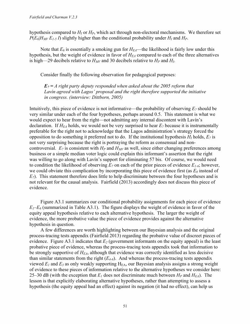
Fairfield and Charman V.2.3
51
hypothesis compared to HI or HP, which act through non-electoral mechanisms. We therefore set P(E6|HMV E1-5 I) slightly higher than the conditional probability under HI and HP.
Note that E6 is essentially a smoking gun for HEA—the likelihood is fairly low under this hypothesis, but the weight of evidence in favor of HEA compared to each of the three alternatives is high—29 decibels relative to HMV and 30 decibels relative to HP and HI.
Consider finally the following observation for pedagogical purposes:
E7 = A right party deputy responded when asked about the 2005 reform that Lavín agreed with Lagos’ proposal and the right therefore supported the initiative in congress. (interview: Dittborn, 2005)
Intuitively, this piece of evidence is not informative—the probability of observing E7 should be very similar under each of the four hypotheses, perhaps around 0.5. This statement is what we would expect to hear from the right—not admitting any internal discontent with Lavín’s declaration. If HEA holds, we would not be very surprised to hear E7 because it is instrumentally preferable for the right not to acknowledge that the Lagos administration’s strategy forced the opposition to do something it preferred not to do. If the institutional hypothesis HI holds, E7 is not very surprising because the right is portraying the reform as consensual and non-controversial. E7 is consistent with HP and HMV as well, since either changing preferences among business or a simple median voter logic could explain this informant’s assertion that the right was willing to go along with Lavín’s support for eliminating 57 bis. Of course, we would need to condition the likelihood of observing E7 on each of the prior pieces of evidence E1-6; however, we could obviate this complication by incorporating this piece of evidence first (as E0 instead of E7). This statement therefore does little to help discriminate between the four hypotheses and is not relevant for the causal analysis. Fairfield (2013) accordingly does not discuss this piece of evidence.
Figure A3.1 summarizes our conditional probability assignments for each piece of evidence E1–E6 (summarized in Table A3.1). The figure displays the weight of evidence in favor of the equity appeal hypothesis relative to each alternative hypothesis. The larger the weight of evidence, the more probative value the piece of evidence provides against the alternative hypothesis in question.
A few differences are worth highlighting between our Bayesian analysis and the original process-tracing tests appendix (Fairfield 2013) regarding the probative value of discreet pieces of evidence. Figure A3.1 indicates that E2 (government informants on the equity appeal) is the least probative piece of evidence, whereas the process-tracing tests appendix took that information to be strongly supportive of HEA, although that evidence was correctly identified as less decisive than similar statements from the right (E4-6). And whereas the process-tracing tests appendix viewed E1 and E3 as only weakly supporting HEA, our Bayesian analysis assigns a strong weight of evidence to these pieces of information relative to the alternative hypotheses we consider here: 25–30 dB (with the exception that E1 does not discriminate much between HP and HEA). The lesson is that explicitly elaborating alternative hypotheses, rather than attempting to assess a hypothesis (the equity appeal had an effect) against its negation (it had no effect), can help us
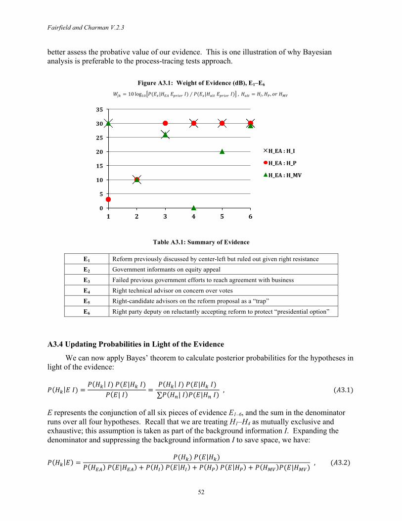
Fairfield and Charman V.2.3
52
better assess the probative value of our evidence. This is one illustration of why Bayesian analysis is preferable to the process-tracing tests approach.
Figure A3.1: Weight of Evidence (dB), E1–E6
𝑊!" = 10 log!" 𝑃(𝐸!|𝐻!" 𝐸!"#$" 𝐼) ∕ 𝑃(𝐸!|𝐻!"# 𝐸!"#$" 𝐼) , 𝐻!"# = 𝐻! ,𝐻! , 𝑜𝑟 𝐻!"
Table A3.1: Summary of Evidence
E1 Reform previously discussed by center-left but ruled out given right resistance E2 Government informants on equity appeal E3 Failed previous government efforts to reach agreement with business E4 Right technical advisor on concern over votes E5 Right-candidate advisors on the reform proposal as a “trap” E6 Right party deputy on reluctantly accepting reform to protect “presidential option”
A3.4 Updating Probabilities in Light of the Evidence
We can now apply Bayes’ theorem to calculate posterior probabilities for the hypotheses in light of the evidence:
𝑃 𝐻! 𝐸 𝐼) =𝑃 𝐻! 𝐼) 𝑃(𝐸|𝐻! 𝐼)
𝑃 𝐸| 𝐼=
𝑃 𝐻! 𝐼) 𝑃(𝐸|𝐻! 𝐼) ∑𝑃 𝐻!| 𝐼 𝑃(𝐸|𝐻! 𝐼)
, (𝐴3.1)
E represents the conjunction of all six pieces of evidence E1–6, and the sum in the denominator runs over all four hypotheses. Recall that we are treating H1–H4 as mutually exclusive and exhaustive; this assumption is taken as part of the background information I. Expanding the denominator and suppressing the background information I to save space, we have:
𝑃 𝐻! 𝐸 =𝑃(𝐻!) 𝑃(𝐸|𝐻!)
𝑃 𝐻!" 𝑃 𝐸|𝐻!" + 𝑃 𝐻! 𝑃 𝐸 𝐻! + 𝑃 𝐻! 𝑃 𝐸 𝐻! + 𝑃 𝐻!" 𝑃(𝐸|𝐻!") , (𝐴3.2)
0
5
10
15
20
25
30
35
1 2 3 4 5 6
H_EA : H_I
H_EA : H_P
H_EA : H_MV
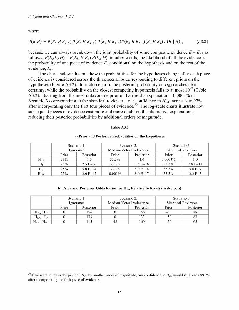
Fairfield and Charman V.2.3
53
where 𝑃 𝐸 𝐻 = 𝑃 𝐸6 𝐻 𝐸1–5 𝑃 𝐸5 𝐻 𝐸1–4 𝑃 𝐸4 𝐻 𝐸1–3 𝑃 𝐸3 𝐻 𝐸1–2 𝐸2 𝐻 𝐸1 𝑃 𝐸! 𝐻 , (𝐴3.3) because we can always break down the joint probability of some composite evidence E = Ea b as follows: P(Ea Eb|H) = P(Eb |H Ea) P(Ea |H), in other words, the likelihood of all the evidence is the probability of one piece of evidence Ea conditional on the hypothesis and on the rest of the evidence, Eb.
The charts below illustrate how the probabilities for the hypotheses change after each piece of evidence is considered across the three scenarios corresponding to different priors on the hypotheses (Figure A3.2). In each scenario, the posterior probability on HEA reaches near certainty, while the probability on the closest competing hypothesis falls to at most 10–7 (Table A3.2). Starting from the most unfavorable prior on Fairfield’s explanation—0.0003% in Scenario 3 corresponding to the skeptical reviewer—our confidence in HEA increases to 97% after incorporating only the first four pieces of evidence.30 The log-scale charts illustrate how subsequent pieces of evidence cast more and more doubt on the alternative explanations, reducing their posterior probabilities by additional orders of magnitude.
Table A3.2
a) Prior and Posterior Probabilities on the Hypotheses
Scenario 1: Ignorance
Scenario 2: Median-Voter Irrelevance
Scenario 3: Skeptical Reviewer
Prior Posterior Prior Posterior Prior Posterior HEA 25% 1.0 33.3% 1.0 0.0003% 1.0 HI 25% 2.5 E–16 33.3% 2.5 E–16 33.3% 2.8 E–11 HP 25% 5.0 E–14 33.3% 5.0 E–14 33.3% 5.6 E–9
HMV 25% 3.0 E–12 0.001% 9.0 E–17 33.3% 3.3 E–7
b) Prior and Posterior Odds Ratios for HEA Relative to Rivals (in decibels)
Scenario 1:
Ignorance Scenario 2:
Median-Voter Irrelevance Scenario 3:
Skeptical Reviewer Prior Posterior Prior Posterior Prior Posterior
HEA : HI 0 156 0 156 –50 106 HEA : HP 0 133 0 133 –50 83
HEA : HMV 0 115 45 160 –50 65
30If we were to lower the prior on HEA by another order of magnitude, our confidence in HEA would still reach 99.7% after incorporating the fifth piece of evidence.
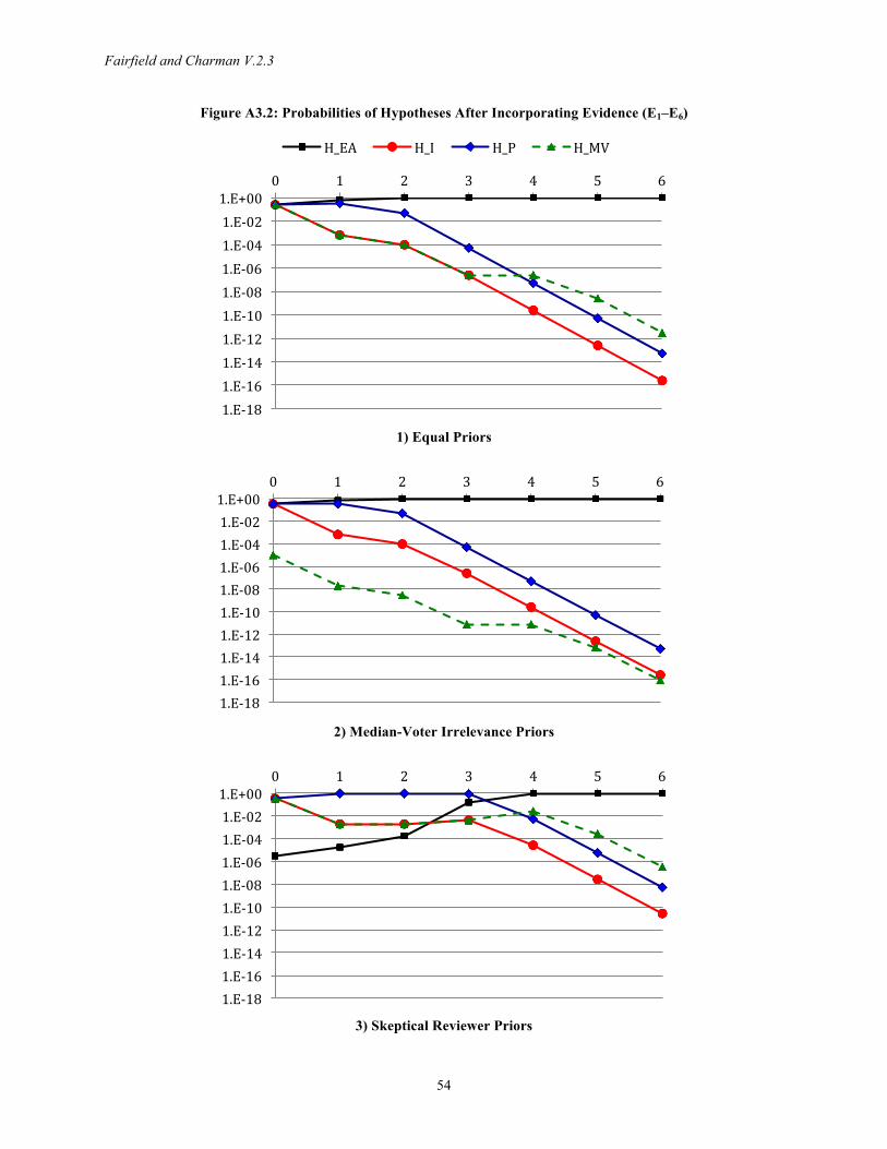
Fairfield and Charman V.2.3
54
Figure A3.2: Probabilities of Hypotheses After Incorporating Evidence (E1–E6)
1) Equal Priors
2) Median-Voter Irrelevance Priors
3) Skeptical Reviewer Priors
1.E-‐18 1.E-‐16 1.E-‐14 1.E-‐12 1.E-‐10 1.E-‐08 1.E-‐06 1.E-‐04 1.E-‐02 1.E+00
0 1 2 3 4 5 6
H_EA H_I H_P H_MV
1.E-‐18 1.E-‐16 1.E-‐14 1.E-‐12 1.E-‐10 1.E-‐08 1.E-‐06 1.E-‐04 1.E-‐02 1.E+00
0 1 2 3 4 5 6
1.E-‐18 1.E-‐16 1.E-‐14 1.E-‐12 1.E-‐10 1.E-‐08 1.E-‐06 1.E-‐04 1.E-‐02 1.E+00
0 1 2 3 4 5 6
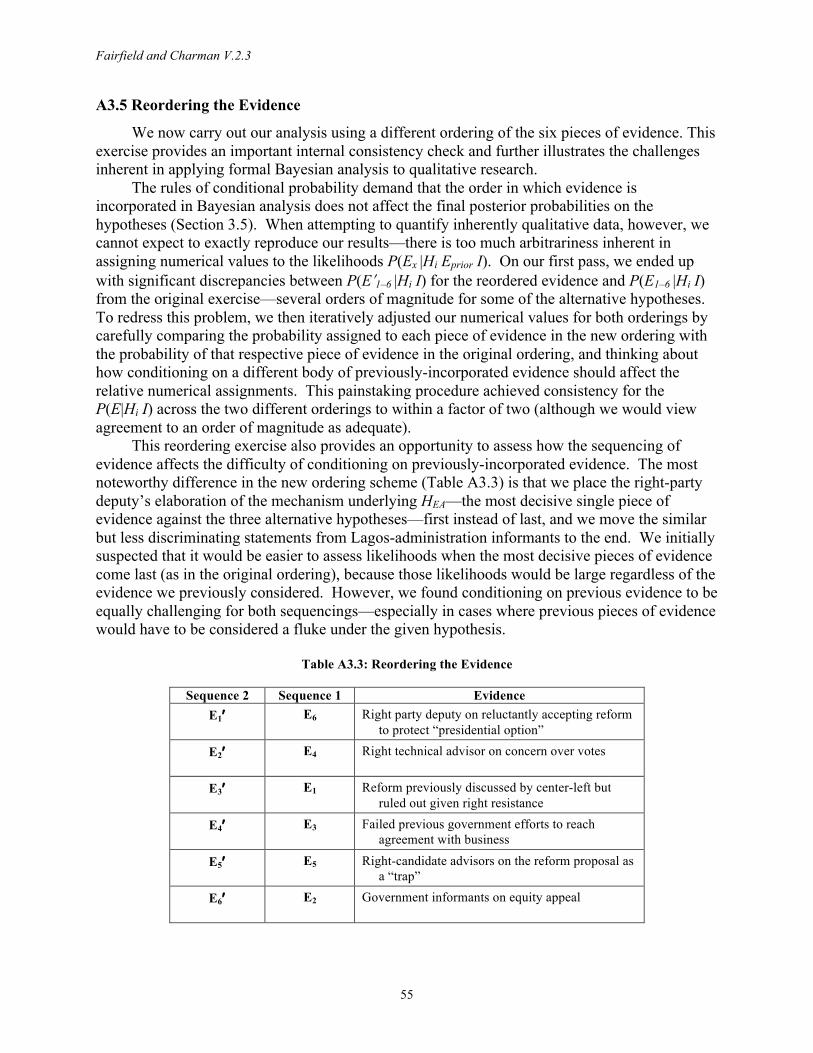
Fairfield and Charman V.2.3
55
A3.5 Reordering the Evidence
We now carry out our analysis using a different ordering of the six pieces of evidence. This exercise provides an important internal consistency check and further illustrates the challenges inherent in applying formal Bayesian analysis to qualitative research.
The rules of conditional probability demand that the order in which evidence is incorporated in Bayesian analysis does not affect the final posterior probabilities on the hypotheses (Section 3.5). When attempting to quantify inherently qualitative data, however, we cannot expect to exactly reproduce our results—there is too much arbitrariness inherent in assigning numerical values to the likelihoods P(Ex |Hi Eprior I). On our first pass, we ended up with significant discrepancies between P(Eʹ′1–6 |Hi I) for the reordered evidence and P(E1–6 |Hi I) from the original exercise—several orders of magnitude for some of the alternative hypotheses. To redress this problem, we then iteratively adjusted our numerical values for both orderings by carefully comparing the probability assigned to each piece of evidence in the new ordering with the probability of that respective piece of evidence in the original ordering, and thinking about how conditioning on a different body of previously-incorporated evidence should affect the relative numerical assignments. This painstaking procedure achieved consistency for the P(E|Hi I) across the two different orderings to within a factor of two (although we would view agreement to an order of magnitude as adequate).
This reordering exercise also provides an opportunity to assess how the sequencing of evidence affects the difficulty of conditioning on previously-incorporated evidence. The most noteworthy difference in the new ordering scheme (Table A3.3) is that we place the right-party deputy’s elaboration of the mechanism underlying HEA—the most decisive single piece of evidence against the three alternative hypotheses—first instead of last, and we move the similar but less discriminating statements from Lagos-administration informants to the end. We initially suspected that it would be easier to assess likelihoods when the most decisive pieces of evidence come last (as in the original ordering), because those likelihoods would be large regardless of the evidence we previously considered. However, we found conditioning on previous evidence to be equally challenging for both sequencings—especially in cases where previous pieces of evidence would have to be considered a fluke under the given hypothesis.
Table A3.3: Reordering the Evidence
Sequence 2 Sequence 1 Evidence E1ʹ′ E6 Right party deputy on reluctantly accepting reform
to protect “presidential option”
E2ʹ′ E4 Right technical advisor on concern over votes
E3ʹ′ E1 Reform previously discussed by center-left but ruled out given right resistance
E4ʹ′ E3 Failed previous government efforts to reach agreement with business
E5ʹ′ E5 Right-candidate advisors on the reform proposal as a “trap”
E6ʹ′ E2 Government informants on equity appeal
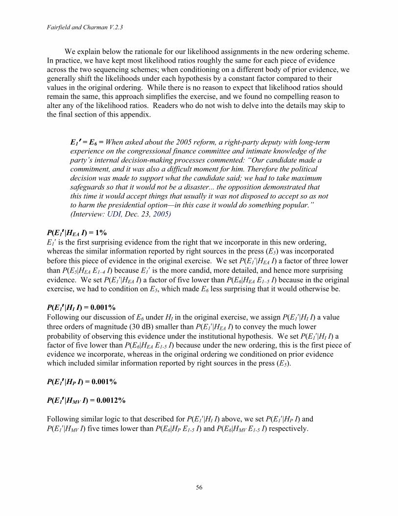
Fairfield and Charman V.2.3
56
We explain below the rationale for our likelihood assignments in the new ordering scheme. In practice, we have kept most likelihood ratios roughly the same for each piece of evidence across the two sequencing schemes; when conditioning on a different body of prior evidence, we generally shift the likelihoods under each hypothesis by a constant factor compared to their values in the original ordering. While there is no reason to expect that likelihood ratios should remain the same, this approach simplifies the exercise, and we found no compelling reason to alter any of the likelihood ratios. Readers who do not wish to delve into the details may skip to the final section of this appendix.
E1ʹ′ = E6 = When asked about the 2005 reform, a right-party deputy with long-term experience on the congressional finance committee and intimate knowledge of the party’s internal decision-making processes commented: “Our candidate made a commitment, and it was also a difficult moment for him. Therefore the political decision was made to support what the candidate said; we had to take maximum safeguards so that it would not be a disaster... the opposition demonstrated that this time it would accept things that usually it was not disposed to accept so as not to harm the presidential option—in this case it would do something popular.” (Interview: UDI, Dec. 23, 2005)
P(E1ʹ′ |HEA I) = 1% E1ʹ′ is the first surprising evidence from the right that we incorporate in this new ordering, whereas the similar information reported by right sources in the press (E5) was incorporated before this piece of evidence in the original exercise. We set P(E1ʹ′|HEA I) a factor of three lower than P(E5|HEA E1–4 I) because E1ʹ′ is the more candid, more detailed, and hence more surprising evidence. We set P(E1ʹ′|HEA I) a factor of five lower than P(E6|HEA E1–5 I) because in the original exercise, we had to condition on E5, which made E6 less surprising that it would otherwise be. P(E1ʹ′ |HI I) = 0.001% Following our discussion of E6 under HI in the original exercise, we assign P(E1ʹ′|HI I) a value three orders of magnitude (30 dB) smaller than P(E1ʹ′|HEA I) to convey the much lower probability of observing this evidence under the institutional hypothesis. We set P(E1ʹ′|HI I) a factor of five lower than P(E6|HEA E1-5 I) because under the new ordering, this is the first piece of evidence we incorporate, whereas in the original ordering we conditioned on prior evidence which included similar information reported by right sources in the press (E5). P(E1ʹ′ |HP I) = 0.001% P(E1ʹ′ |HMV I) = 0.0012% Following similar logic to that described for P(E1ʹ′|HI I) above, we set P(E1ʹ′|HP I) and P(E1ʹ′|HMV I) five times lower than P(E6|HP E1-5 I) and P(E6|HMV E1-5 I) respectively.
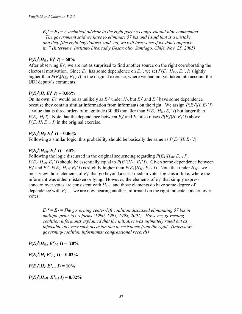
Fairfield and Charman V.2.3
57
E2ʹ′ = E4 = A technical advisor to the right party’s congressional bloc commented: “The government said we have to eliminate 57 bis and I said that is a mistake, and they [the right legislators] said ‘no, we will lose votes if we don’t approve it.’” (Interview, Instituto Libertad y Desarrollo, Santiago, Chile, Nov. 25, 2005)
P(E2ʹ′ |HEA E1ʹ′ I) = 60% After observing E1ʹ′, we are not as surprised to find another source on the right corroborating the electoral motivation. Since E2ʹ′ has some dependence on E1ʹ′, we set P(E2ʹ′|HEA, E1ʹ′, I) slightly higher than P(E4|HEA E1-3 I) in the original exercise, where we had not yet taken into account the UDI deputy’s comments. P(E2ʹ′ |HI E1ʹ′ I) = 0.06% On its own, E2ʹ′ would be as unlikely as E1ʹ′ under HI, but E2ʹ′ and E1ʹ′ have some dependence because they contain similar information from informants on the right. We assign P(E2ʹ′|HI E1ʹ′ I) a value that is three orders of magnitude (30 dB) smaller than P(E2ʹ′|HEA E1ʹ′ I) but larger than P(E1ʹ′|HI I). Note that the dependence between E2ʹ′ and E1ʹ′ also raises P(E2ʹ′|HI E1ʹ′ I) above P(E4|HI E1-3 I) in the original exercise. P(E2ʹ′ |HP E1ʹ′ I) = 0.06% Following a similar logic, this probability should be basically the same as P(E2ʹ′|HI E1ʹ′ I). P(E2ʹ′ |HMV E1ʹ′ I) = 60% Following the logic discussed in the original sequencing regarding P(E4 |HMV E1-3 I), P(E2ʹ′|HMV E1ʹ′ I) should be essentially equal to P(E2ʹ′|HEA E1ʹ′ I). Given some dependence between E2ʹ′ and E1ʹ′, P(E2ʹ′|HMV E1ʹ′ I) is slightly higher than P(E4 |HMV E1-3 I). Note that under HMV, we must view those elements of E1ʹ′ that go beyond a strict median voter logic as a fluke, where the informant was either mistaken or lying. However, the elements of E1ʹ′ that simply express concern over votes are consistent with HMV, and those elements do have some degree of dependence with E2ʹ′ —we are now hearing another informant on the right indicate concern over votes.
E3ʹ′ = E1 = The governing center-left coalition discussed eliminating 57 bis in multiple prior tax reforms (1990, 1995, 1998, 2001). However, governing-coalition informants explained that the initiative was ultimately ruled out as infeasible on every such occasion due to resistance from the right. (Interviews: governing-coalition informants; congressional records)
P(E3ʹ′ |HEA Eʹ′1-2 I) = 20% P(E3ʹ′ |HI Eʹ′1-2 I) = 0.02% P(E3ʹ′ |HP Eʹ′1-2 I) = 10% P(E3ʹ′ |HMV Eʹ′1-2 I) = 0.02%
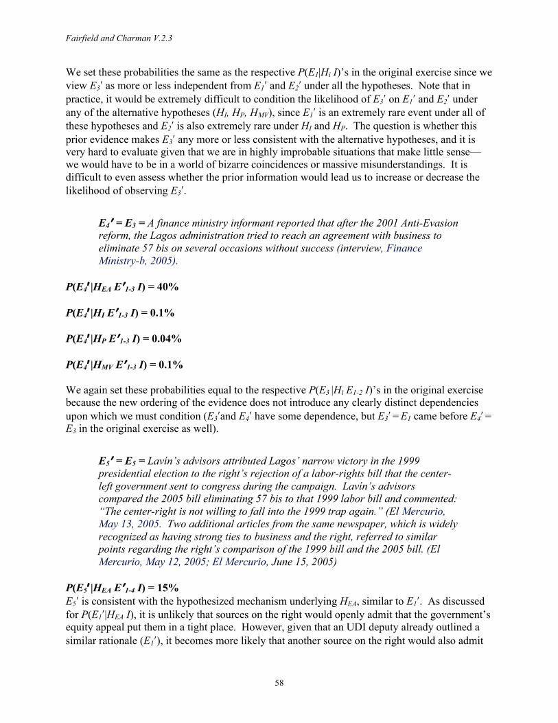
Fairfield and Charman V.2.3
58
We set these probabilities the same as the respective P(E1|Hi I)’s in the original exercise since we view E3ʹ′ as more or less independent from E1ʹ′ and E2ʹ′ under all the hypotheses. Note that in practice, it would be extremely difficult to condition the likelihood of E3ʹ′ on E1ʹ′ and E2ʹ′ under any of the alternative hypotheses (HI, HP, HMV), since E1ʹ′ is an extremely rare event under all of these hypotheses and E2ʹ′ is also extremely rare under HI and HP. The question is whether this prior evidence makes E3ʹ′ any more or less consistent with the alternative hypotheses, and it is very hard to evaluate given that we are in highly improbable situations that make little sense—we would have to be in a world of bizarre coincidences or massive misunderstandings. It is difficult to even assess whether the prior information would lead us to increase or decrease the likelihood of observing E3ʹ′.
E4ʹ′ = E3 = A finance ministry informant reported that after the 2001 Anti-Evasion reform, the Lagos administration tried to reach an agreement with business to eliminate 57 bis on several occasions without success (interview, Finance Ministry-b, 2005).
P(E4ʹ′ |HEA Eʹ′1-3 I) = 40% P(E4ʹ′ |HI Eʹ′1-3 I) = 0.1% P(E4ʹ′ |HP Eʹ′1-3 I) = 0.04% P(E4ʹ′ |HMV Eʹ′1-3 I) = 0.1% We again set these probabilities equal to the respective P(E3 |Hi E1-2 I)’s in the original exercise because the new ordering of the evidence does not introduce any clearly distinct dependencies upon which we must condition (E3ʹ′and E4ʹ′ have some dependence, but E3ʹ′ = E1 came before E4ʹ′ = E3 in the original exercise as well).
E5ʹ′ = E5 = Lavín’s advisors attributed Lagos’ narrow victory in the 1999 presidential election to the right’s rejection of a labor-rights bill that the center-left government sent to congress during the campaign. Lavín’s advisors compared the 2005 bill eliminating 57 bis to that 1999 labor bill and commented: “The center-right is not willing to fall into the 1999 trap again.” (El Mercurio, May 13, 2005. Two additional articles from the same newspaper, which is widely recognized as having strong ties to business and the right, referred to similar points regarding the right’s comparison of the 1999 bill and the 2005 bill. (El Mercurio, May 12, 2005; El Mercurio, June 15, 2005)
P(E5ʹ′ |HEA Eʹ′1-4 I) = 15% E5ʹ′ is consistent with the hypothesized mechanism underlying HEA, similar to E1ʹ′. As discussed for P(E1ʹ′|HEA I), it is unlikely that sources on the right would openly admit that the government’s equity appeal put them in a tight place. However, given that an UDI deputy already outlined a similar rationale (E1ʹ′), it becomes more likely that another source on the right would also admit
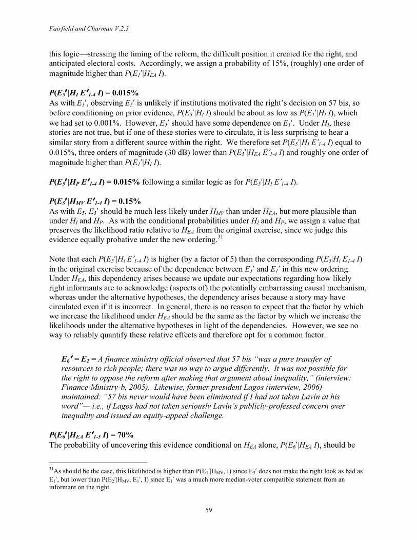
Fairfield and Charman V.2.3
59
this logic—stressing the timing of the reform, the difficult position it created for the right, and anticipated electoral costs. Accordingly, we assign a probability of 15%, (roughly) one order of magnitude higher than P(E1ʹ′|HEA I). P(E5ʹ′ |HI Eʹ′1-4 I) = 0.015% As with E1ʹ′, observing E5ʹ′ is unlikely if institutions motivated the right’s decision on 57 bis, so before conditioning on prior evidence, P(E5ʹ′|HI I) should be about as low as P(E1ʹ′|HI I), which we had set to 0.001%. However, E5ʹ′ should have some dependence on E1ʹ′. Under HI, these stories are not true, but if one of these stories were to circulate, it is less surprising to hear a similar story from a different source within the right. We therefore set P(E5ʹ′|HI Eʹ′1-4 I) equal to 0.015%, three orders of magnitude (30 dB) lower than P(E5ʹ′|HEA Eʹ′1-4 I) and roughly one order of magnitude higher than P(E1ʹ′|HI I). P(E5ʹ′ |HP Eʹ′1-4 I) = 0.015% following a similar logic as for P(E5ʹ′|HI Eʹ′1-4 I). P(E5ʹ′ |HMV Eʹ′1-4 I) = 0.15% As with E5, E5ʹ′ should be much less likely under HMV than under HEA, but more plausible than under HI and HP. As with the conditional probabilities under HI and HP, we assign a value that preserves the likelihood ratio relative to HEA from the original exercise, since we judge this evidence equally probative under the new ordering.31 Note that each P(E5ʹ′|Hi Eʹ′1-4 I) is higher (by a factor of 5) than the corresponding P(E5|Hi E1-4 I) in the original exercise because of the dependence between E5ʹ′ and E1ʹ′ in this new ordering. Under HEA, this dependency arises because we update our expectations regarding how likely right informants are to acknowledge (aspects of) the potentially embarrassing causal mechanism, whereas under the alternative hypotheses, the dependency arises because a story may have circulated even if it is incorrect. In general, there is no reason to expect that the factor by which we increase the likelihood under HEA should be the same as the factor by which we increase the likelihoods under the alternative hypotheses in light of the dependencies. However, we see no way to reliably quantify these relative effects and therefore opt for a common factor.
E6ʹ′ = E2 = A finance ministry official observed that 57 bis “was a pure transfer of resources to rich people; there was no way to argue differently. It was not possible for the right to oppose the reform after making that argument about inequality,” (interview: Finance Ministry-b, 2005). Likewise, former president Lagos (interview, 2006) maintained: “57 bis never would have been eliminated if I had not taken Lavín at his word”— i.e., if Lagos had not taken seriously Lavín’s publicly-professed concern over inequality and issued an equity-appeal challenge.
P(E6ʹ′ |HEA Eʹ′1-5 I) = 70% The probability of uncovering this evidence conditional on HEA alone, P(E6ʹ′|HEA I), should be
31As should be the case, this likelihood is higher than P(E1ʹ′|HMV, I) since E5ʹ′ does not make the right look as bad as E1ʹ′, but lower than P(E2ʹ′|HMV, E1ʹ′, I) since E1ʹ′ was a much more median-voter compatible statement from an informant on the right.
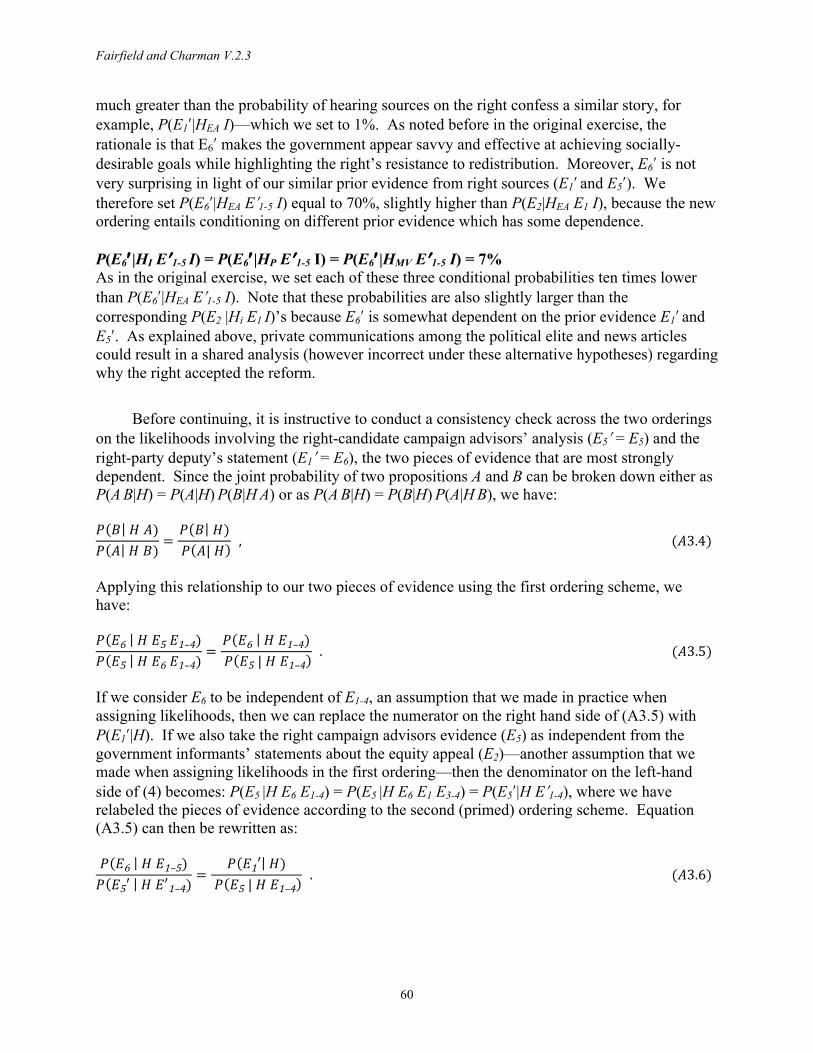
Fairfield and Charman V.2.3
60
much greater than the probability of hearing sources on the right confess a similar story, for example, P(E1ʹ′|HEA I)—which we set to 1%. As noted before in the original exercise, the rationale is that E6ʹ′ makes the government appear savvy and effective at achieving socially-desirable goals while highlighting the right’s resistance to redistribution. Moreover, E6ʹ′ is not very surprising in light of our similar prior evidence from right sources (E1ʹ′ and E5ʹ′). We therefore set P(E6ʹ′|HEA Eʹ′1-5 I) equal to 70%, slightly higher than P(E2|HEA E1 I), because the new ordering entails conditioning on different prior evidence which has some dependence. P(E6ʹ′ |HI Eʹ′1-5 I) = P(E6ʹ′ |HP Eʹ′1-5 I) = P(E6ʹ′ |HMV Eʹ′1-5 I) = 7% As in the original exercise, we set each of these three conditional probabilities ten times lower than P(E6ʹ′|HEA Eʹ′1-5 I). Note that these probabilities are also slightly larger than the corresponding P(E2 |Hi E1 I)’s because E6ʹ′ is somewhat dependent on the prior evidence E1ʹ′ and E5ʹ′. As explained above, private communications among the political elite and news articles could result in a shared analysis (however incorrect under these alternative hypotheses) regarding why the right accepted the reform.
Before continuing, it is instructive to conduct a consistency check across the two orderings on the likelihoods involving the right-candidate campaign advisors’ analysis (E5ʹ′ = E5) and the right-party deputy’s statement (E1ʹ′ = E6), the two pieces of evidence that are most strongly dependent. Since the joint probability of two propositions A and B can be broken down either as P(A B|H) = P(A|H) P(B|H A) or as P(A B|H) = P(B|H) P(A|H B), we have: 𝑃 𝐵 𝐻 𝐴)𝑃 𝐴 𝐻 𝐵)
=𝑃 𝐵 𝐻) 𝑃 𝐴| 𝐻
, (𝐴3.4)
Applying this relationship to our two pieces of evidence using the first ordering scheme, we have: 𝑃 𝐸6 𝐻 𝐸5 𝐸1–4)𝑃 𝐸5 𝐻 𝐸6 𝐸1–4)
=𝑃 𝐸6 𝐻 𝐸1–4) 𝑃 𝐸5 | 𝐻 𝐸1–4
. (𝐴3.5)
If we consider E6 to be independent of E1-4, an assumption that we made in practice when assigning likelihoods, then we can replace the numerator on the right hand side of (A3.5) with P(E1ʹ′|H). If we also take the right campaign advisors evidence (E5) as independent from the government informants’ statements about the equity appeal (E2)—another assumption that we made when assigning likelihoods in the first ordering—then the denominator on the left-hand side of (4) becomes: P(E5 |H E6 E1-4) = P(E5 |H E6 E1 E3-4) = P(E5ʹ′|H Eʹ′1-4), where we have relabeled the pieces of evidence according to the second (primed) ordering scheme. Equation (A3.5) can then be rewritten as: 𝑃 𝐸6 𝐻 𝐸1–5)𝑃 𝐸5′ 𝐻 𝐸′1–4)
=𝑃 𝐸1′ 𝐻)
𝑃 𝐸5 | 𝐻 𝐸1–4 . (𝐴3.6)
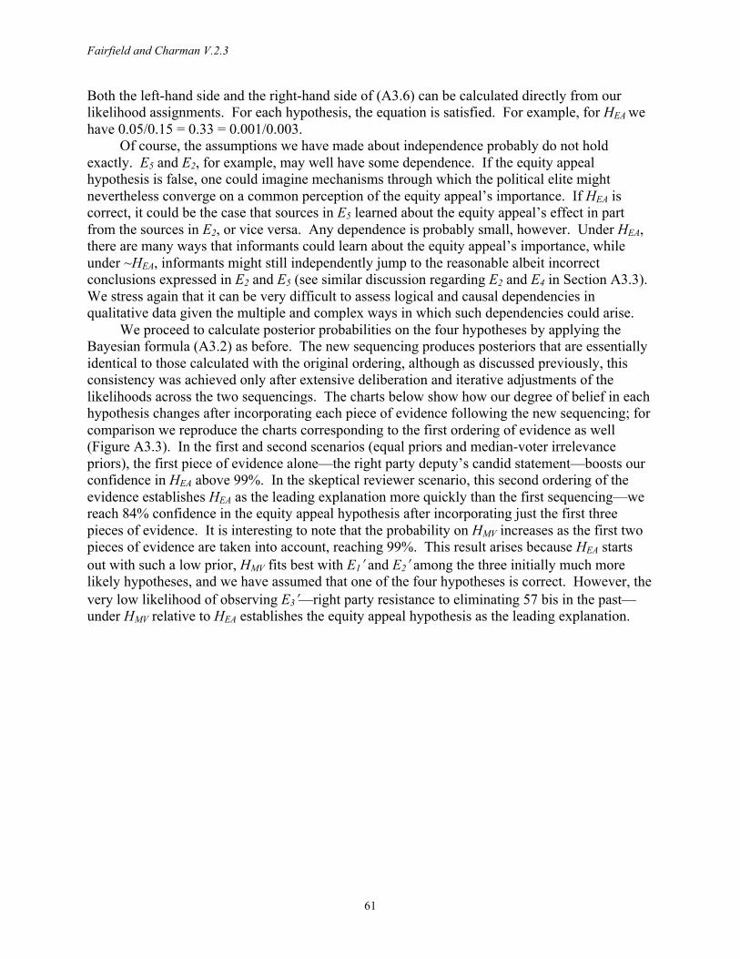
Fairfield and Charman V.2.3
61
Both the left-hand side and the right-hand side of (A3.6) can be calculated directly from our likelihood assignments. For each hypothesis, the equation is satisfied. For example, for HEA we have 0.05/0.15 = 0.33 = 0.001/0.003.
Of course, the assumptions we have made about independence probably do not hold exactly. E5 and E2, for example, may well have some dependence. If the equity appeal hypothesis is false, one could imagine mechanisms through which the political elite might nevertheless converge on a common perception of the equity appeal’s importance. If HEA is correct, it could be the case that sources in E5 learned about the equity appeal’s effect in part from the sources in E2, or vice versa. Any dependence is probably small, however. Under HEA, there are many ways that informants could learn about the equity appeal’s importance, while under ~HEA, informants might still independently jump to the reasonable albeit incorrect conclusions expressed in E2 and E5 (see similar discussion regarding E2 and E4 in Section A3.3). We stress again that it can be very difficult to assess logical and causal dependencies in qualitative data given the multiple and complex ways in which such dependencies could arise.
We proceed to calculate posterior probabilities on the four hypotheses by applying the Bayesian formula (A3.2) as before. The new sequencing produces posteriors that are essentially identical to those calculated with the original ordering, although as discussed previously, this consistency was achieved only after extensive deliberation and iterative adjustments of the likelihoods across the two sequencings. The charts below show how our degree of belief in each hypothesis changes after incorporating each piece of evidence following the new sequencing; for comparison we reproduce the charts corresponding to the first ordering of evidence as well (Figure A3.3). In the first and second scenarios (equal priors and median-voter irrelevance priors), the first piece of evidence alone—the right party deputy’s candid statement—boosts our confidence in HEA above 99%. In the skeptical reviewer scenario, this second ordering of the evidence establishes HEA as the leading explanation more quickly than the first sequencing—we reach 84% confidence in the equity appeal hypothesis after incorporating just the first three pieces of evidence. It is interesting to note that the probability on HMV increases as the first two pieces of evidence are taken into account, reaching 99%. This result arises because HEA starts out with such a low prior, HMV fits best with E1ʹ′ and E2ʹ′ among the three initially much more likely hypotheses, and we have assumed that one of the four hypotheses is correct. However, the very low likelihood of observing E3ʹ′—right party resistance to eliminating 57 bis in the past—under HMV relative to HEA establishes the equity appeal hypothesis as the leading explanation.
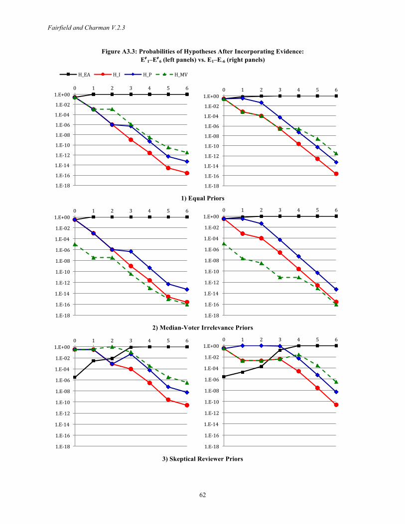
Fairfield and Charman V.2.3
62
Figure A3.3: Probabilities of Hypotheses After Incorporating Evidence: Eʹ′1–Eʹ′6 (left panels) vs. E1–E-6 (right panels)
1) Equal Priors
2) Median-Voter Irrelevance Priors
3) Skeptical Reviewer Priors
1.E-‐18
1.E-‐16
1.E-‐14
1.E-‐12
1.E-‐10
1.E-‐08
1.E-‐06
1.E-‐04
1.E-‐02
1.E+00 0 1 2 3 4 5 6
H_EA H_I H_P H_MV
1.E-‐18
1.E-‐16
1.E-‐14
1.E-‐12
1.E-‐10
1.E-‐08
1.E-‐06
1.E-‐04
1.E-‐02
1.E+00 0 1 2 3 4 5 6
1.E-‐18
1.E-‐16
1.E-‐14
1.E-‐12
1.E-‐10
1.E-‐08
1.E-‐06
1.E-‐04
1.E-‐02
1.E+00 0 1 2 3 4 5 6
1.E-‐18
1.E-‐16
1.E-‐14
1.E-‐12
1.E-‐10
1.E-‐08
1.E-‐06
1.E-‐04
1.E-‐02
1.E+00 0 1 2 3 4 5 6
1.E-‐18
1.E-‐16
1.E-‐14
1.E-‐12
1.E-‐10
1.E-‐08
1.E-‐06
1.E-‐04
1.E-‐02
1.E+00 0 1 2 3 4 5 6
1.E-‐18
1.E-‐16
1.E-‐14
1.E-‐12
1.E-‐10
1.E-‐08
1.E-‐06
1.E-‐04
1.E-‐02
1.E+00 0 1 2 3 4 5 6
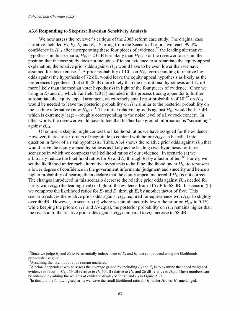
Fairfield and Charman V.2.3
63
A3.6 Responding to Skeptics: Bayesian Sensitivity Analysis
We now assess the reviewer’s critique of the 2005 reform case study. The original case narrative included E1, E2, E5 and E6. Starting from the Scenario 3 priors, we reach 99.4% confidence in HEA after incorporating these four pieces of evidence;32 the leading alternative hypothesis in this scenario, HP, is 23 dB less likely than HEA. For the reviewer to sustain the position that the case study does not include sufficient evidence to substantiate the equity-appeal explanation, the relative prior odds against HEA would have to be even lower than we have assumed for this exercise.33 A prior probability of 10–8 on HEA, corresponding to relative log-odds against the hypothesis of 72 dB, would leave the equity appeal hypothesis as likely as the preferences hypothesis (but still 28 dB more likely than the institutional hypothesis and 17 dB more likely than the median voter hypothesis) in light of the four pieces of evidence. Once we bring in E3 and E4, which Fairfield (2013) included in the process tracing appendix to further substantiate the equity appeal argument, an extremely small prior probability of 10–12 on HEA would be needed to leave the posterior probability on HEA similar to the posterior probability on the leading alternative (now HMV).34 The initial relative log-odds against HEA would be 115 dB, which is extremely large—roughly corresponding to the noise level of a live rock concert. In other words, the reviewer would have to feel that his/her background information is “screaming” against HEA.
Of course, a skeptic might contest the likelihood ratios we have assigned for the evidence. However, there are six orders of magnitude to contend with before HEA can be called into question in favor of a rival hypothesis. Table A3.4 shows the relative prior odds against HEA that would leave the equity appeal hypothesis as likely as the leading rival hypothesis for three scenarios in which we compress the likelihood ratios of our evidence. In scenario (a) we arbitrarily reduce the likelihood ratios for E1 and E3 through E6 by a factor of ten.35 For E2, we set the likelihood under each alternative hypothesis to half the likelihood under HEA to represent a lower degree of confidence in the government informants’ judgment and sincerity and hence a higher probability of hearing them declare that the equity appeal mattered if HEA is not correct. The changes introduced in this scenario decrease the relative prior odds against HEA needed for parity with HMV (the leading rival) in light of the evidence from 115 dB to 68 dB. In scenario (b) we compress the likelihood ratios for E1 and E3 through E6 by another factor of five. This scenario reduces the relative prior odds against HEA required for equivalence with HMV to slightly over 40 dB. However, in scenario (c) where we simultaneously lower the prior on HMV to 0.1% while keeping the priors on HI and HP equal, the posterior probability on HEA remains higher than the rivals until the relative prior odds against HEA compared to HP increase to 58 dB.
32Since we judge E5 and E6 to be essentially independent of E3 and E4, we can proceed using the likelihoods previously assigned. 33Assuming the likelihood ratios remain unaltered. 34A prior-independent way to assess the leverage gained by including E3 and E4 is to examine the added weight of evidence in favor of HEA: 56 dB relative to HI, 60 dB relative to HP, and 26 dB relative to HMV. These numbers can be obtained by adding the weights of evidence displayed for E3 and E4 in Figure A3.1. 35In this and the following scenarios we leave the small likelihood ratio for E1 under HEA vs. HP unchanged.
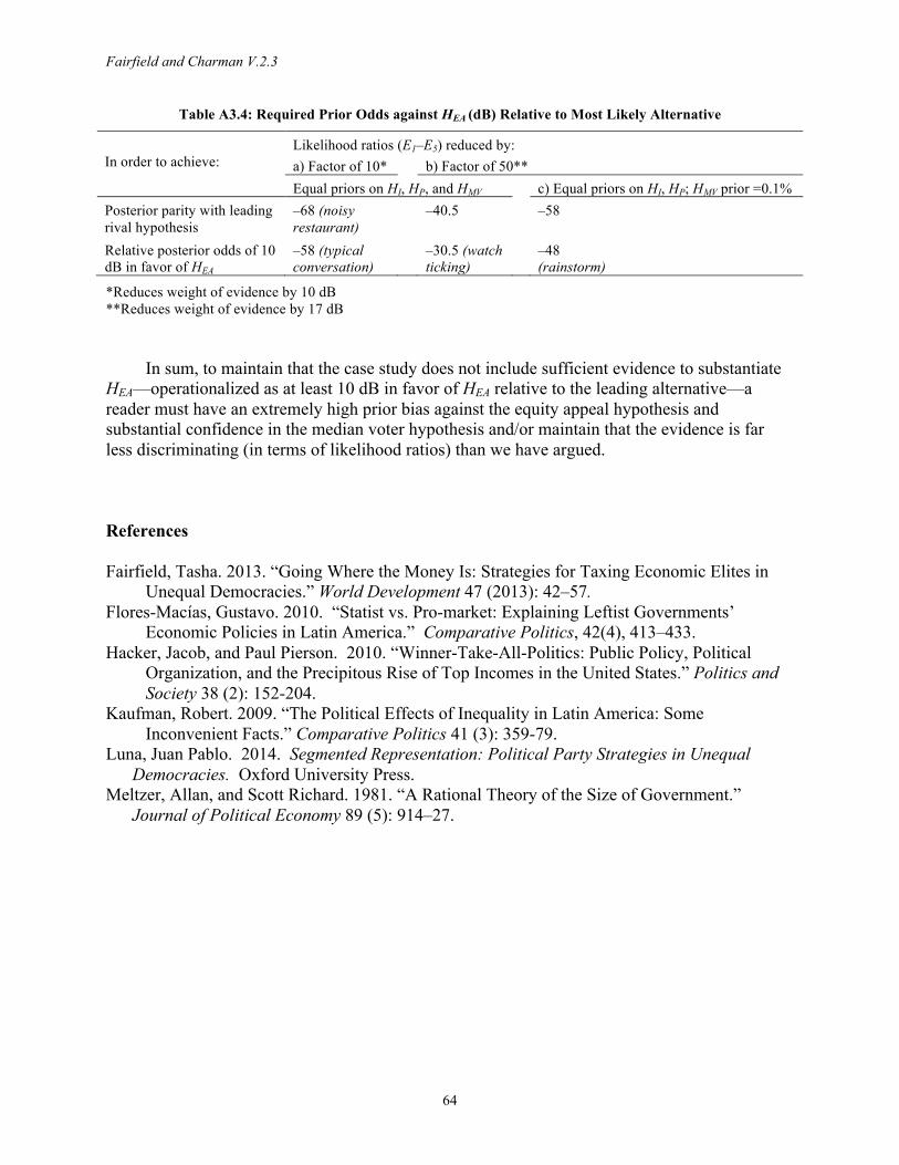
Fairfield and Charman V.2.3
64
Table A3.4: Required Prior Odds against HEA (dB) Relative to Most Likely Alternative
Likelihood ratios (E1–E5) reduced by: In order to achieve: a) Factor of 10* b) Factor of 50**
Equal priors on HI, HP, and HMV c) Equal priors on HI, HP; HMV prior =0.1% Posterior parity with leading rival hypothesis
–68 (noisy restaurant)
–40.5 –58
Relative posterior odds of 10 dB in favor of HEA
–58 (typical conversation)
–30.5 (watch ticking)
–48 (rainstorm)
*Reduces weight of evidence by 10 dB **Reduces weight of evidence by 17 dB
In sum, to maintain that the case study does not include sufficient evidence to substantiate HEA—operationalized as at least 10 dB in favor of HEA relative to the leading alternative—a reader must have an extremely high prior bias against the equity appeal hypothesis and substantial confidence in the median voter hypothesis and/or maintain that the evidence is far less discriminating (in terms of likelihood ratios) than we have argued.
References Fairfield, Tasha. 2013. “Going Where the Money Is: Strategies for Taxing Economic Elites in
Unequal Democracies.” World Development 47 (2013): 42–57. Flores-Macías, Gustavo. 2010. “Statist vs. Pro-market: Explaining Leftist Governments’
Economic Policies in Latin America.” Comparative Politics, 42(4), 413–433. Hacker, Jacob, and Paul Pierson. 2010. “Winner-Take-All-Politics: Public Policy, Political
Organization, and the Precipitous Rise of Top Incomes in the United States.” Politics and Society 38 (2): 152-204.
Kaufman, Robert. 2009. “The Political Effects of Inequality in Latin America: Some Inconvenient Facts.” Comparative Politics 41 (3): 359-79.
Luna, Juan Pablo. 2014. Segmented Representation: Political Party Strategies in Unequal Democracies. Oxford University Press.
Meltzer, Allan, and Scott Richard. 1981. “A Rational Theory of the Size of Government.” Journal of Political Economy 89 (5): 914–27.
Fairfield and Charman V.2.3
65
A4. Case Narrative: Chile’s 2005 Tax Reform Excerpt from Fairfield (2013: 47-49)
Business’s strong political power made it difficult for Chile’s center-left governments to
legislate tax increases in the 1990s and 2000s. Business power arose primarily from organization and partisan ties (Fairfield, 2010). Chile’s prestigious economy-wide business association, the CPC, coordinated lobbying across sectors on sensitive issues like taxation, which business often portrayed as confiscation of property. Further, business was a core constituency for the two right parties, especially the UDI. The UDI’s neoliberal, low-tax policy positions drew electoral and financial support from business owners (Luna, 2010). The UDI and dominant business groups were also linked through common origins in the Pinochet dictatorship; government technocrats who later joined the UDI were often board members of business groups that benefited from privatization (Schamis, 1999; Silva, 1996). The right, which was essentially tied with the center-left in the senate during Lagos’ administration (2000–05), often took instruction on tax policy directly from business, and business and the right mounted coordinated opposition (interviews: Finance Ministry-a, 2007; Tax Agency, 2005). Increasing taxes therefore en- tailed costly political battles.
When center-left governments sought to increase the low direct tax burden born by economic elites, they employed multiple strategies, among which equity appeals were often prominent. Equity appeals created political space for incremental advances despite strong business power. As the two cases illustrate, equity appeals undermined business-right opposition more effectively during electoral periods, particularly when inequality became a salient campaign issue.
…
Legitimating appeals helped the government legislate another income-tax base-broadening measure in 2005. Given the unusually high salience of inequality during a presidential campaign, vertical equity appeals generated much stronger electoral incentives for the right to deviate from its core business constituency’s preferences.
The tax benefit known as “57 bis,” inherited from the dictatorship, constituted a perpetual government subsidy for owners of new-issue stocks, most of whom belonged to the wealthiest percentile of taxpayers. The Lagos administration considered eliminating 57 bis in the Anti-Evasion reform, but it was judged infeasible given strong business-right resistance (interview, Finance Ministry-c, 2005). Efforts to eliminate the exemption in the 1990s also failed.
An opportunity for reform arose in 2005 due to unanticipated electoral competition from the right on the issue of inequality. When Chile’s Catholic bishops forcefully denounced the country’s persistent inequality, right-coalition presidential candidate Lavín blamed lack of progress on the center-left: “Inequality, Mr. President, continues. ...There is a Chile that grows, but it is for the few, and the great majority have not yet benefited,” (El Mercurio, 2005a). Inequality became the central campaign issue during the following weeks. President Lagos responded with a challenge: “The infamous article 57 bis represents a tremendous support for inequality. . . Instead of just talking, why don’t we agree to eliminate 57 bis in less than 24 hours?” (El Mercurio, 2005b).
This vertical equity appeal proved highly successful. In contrast to the Anti-Evasion reform, debate on 57 bis was minimal. Lavín accepted the government’s challenge: “…we are all for equity. Let’s do it,” (El Mercurio, 2005c), and right legislators followed his lead,
Fairfield and Charman V.2.3
66
disregarding business’s policy preferences. The bill received nearly unanimous congressional approval.
The salience of inequality during the campaign raised the anticipated political costs to the right of defending business interests. Opposing the reform would have undermined Lavín’s credibility and validated the government’s claim that the right was the main obstacle to reducing inequality in Chile. With only six months until the election and public attention focused on inequality, voters might well have remembered the coalition’s policy position and punished Lavín at the polls. Lavín ’s advisors attributed Lagos’ narrow 1999 victory to the right’s rejection of a popular labor-rights bill sent to congress during the campaign; this episode weighed heavily in the right’s analysis of the 2005 reform (El Mercurio, 2005d, 2005e). Comparing the two reforms, a Lavín advisor declared: “The center-right is not willing to fall into the 1999 trap again,” (El Mercurio, 2005e). Meanwhile, framing the tax in- crease as hurting the middle class, a tactic regularly used by the right, was not feasible because the reform patently targeted elites. Tax agency data showed that 0.5% of adults received 72% of the tax expenditure associated with 57 bis. As a government informant recalled: “it was a pure transfer of resources to rich people; there was no way to argue differently. …It was not possible for the right to oppose the reform after making that argument about inequality,” (interview, Finance Ministry-b, 2005). An UDI (interview, 2005) informant candidly acknowledged that electoral concerns motivated the right to accept the reform: “the opposition demonstrated that this time it would accept things that usually it was not disposed to accept so as not to harm the presidential option—in this case it would do something popular, perhaps populist.” The counterfactual therefore seems clear: had the government attempted to eliminate 57 bis without the high-profile equity appeal, the right would have blocked the reform as it had on multiple prior occasions.