formal reasoning about systems biology using theorem...

RESEARCH ARTICLE

Formal reasoning about systems biology

using theorem proving

Adnan Rashid1*, Osman Hasan1, Umair Siddique2, Sofiène Tahar2

1 School of Electrical Engineering and Computer Science, National University of Sciences and Technology,

Islamabad, Pakistan, 2 Department of Electrical and Computer Engineering, Concordia University, Montreal,

QC, Canada

* [email protected]

Abstract

System biology provides the basis to understand the behavioral properties of complex bio-

logical organisms at different levels of abstraction. Traditionally, analysing systems biology

based models of various diseases have been carried out by paper-and-pencil based proofs

and simulations. However, these methods cannot provide an accurate analysis, which is a

serious drawback for the safety-critical domain of human medicine. In order to overcome

these limitations, we propose a framework to formally analyze biological networks and path-

ways. In particular, we formalize the notion of reaction kinetics in higher-order logic and for-

mally verify some of the commonly used reaction based models of biological networks using

the HOL Light theorem prover. Furthermore, we have ported our earlier formalization of

Zsyntax, i.e., a deductive language for reasoning about biological networks and pathways,

from HOL4 to the HOL Light theorem prover to make it compatible with the above-men-

tioned formalization of reaction kinetics. To illustrate the usefulness of the proposed frame-

work, we present the formal analysis of three case studies, i.e., the pathway leading to TP53

Phosphorylation, the pathway leading to the death of cancer stem cells and the tumor

growth based on cancer stem cells, which is used for the prognosis and future drug designs

to treat cancer patients.

Introduction

The discovery and design of effective drugs for infectious and chronic biological diseases, like

cancer and cerebral malaria, require a deep understanding of behaviorial and structural char-

acteristics of underlying biological entities (e.g., cells, molecules and enzymes). Traditional

approaches, which rely on verbal and personal intuitions without concrete logical explanations

of biological phenomena, often fail to provide a complete understanding of the behavior of

such diseases, mainly due to the complex interactions of molecules connected through a chain

of reactions. Systems biology [1] overcomes these limitations by integrating mathematical

modeling and high-speed computing machines in the understanding of biological processes

and thus provides the ability to predict the effect of potential drugs for the treatment of chronic

diseases. System biology is widely used to model the biological processes as pathways or

PLOS ONE | https://doi.org/10.1371/journal.pone.0180179 July 3, 2017 1 / 27

a1111111111

a1111111111

a1111111111

a1111111111

a1111111111

OPENACCESS

Citation: Rashid A, Hasan O, Siddique U, Tahar S

(2017) Formal reasoning about systems biology

using theorem proving. PLoS ONE 12(7):

e0180179. https://doi.org/10.1371/journal.

pone.0180179

Editor: Andrew Adamatzky, University of the West

of England, UNITED KINGDOM

Received: December 20, 2016

Accepted: June 12, 2017

Published: July 3, 2017

Copyright: © 2017 Rashid et al. This is an open

access article distributed under the terms of the

Creative Commons Attribution License, which

permits unrestricted use, distribution, and

reproduction in any medium, provided the original

author and source are credited.

Data Availability Statement: All relevant data are

within the paper and its Supporting Information

files. http://save.seecs.nust.edu.pk/projects/

sbiology/.

Funding: The author(s) received no specific

funding for this work.

Competing interests: The authors have declared

that no competing interests exist.

https://doi.org/10.1371/journal.pone.0180179

http://crossmark.crossref.org/dialog/?doi=10.1371/journal.pone.0180179&domain=pdf&date_stamp=2017-07-03








http://creativecommons.org/licenses/by/4.0/

http://save.seecs.nust.edu.pk/projects/sbiology/


networks. Some of the examples are signaling pathways and protein-protein interaction net-

works [2]. These biological networks such as gene regulatory networks (GRNs) or biological

regulatory networks (BRNs) [3], are analysed using the principles of molecular biology. This

analysis, in turn, plays an important role for the investigation of the treatment of various

human infectious diseases as well as future drug design targets. For example, the BRNs analysis

has been recently used for the prediction of treatment decisions for sepsis patients [4].

Traditionally, biologists analyze biological organisms (or different diseases) using wet-lab

experiments [5, 6]. These experiments cannot provide reliable analysis due to their inability to

accurately characterize the complex biological processes in an experimental setting. Moreover,

the experiments take a long execution time and often require an expensive experimental setup.

One of the other techniques used for the deduction of molecular reactions is the paper-and-

pencil proof method (e.g. Boolean modeling [7] or kinetic logic [8]). But the manual proofs in

paper-and-pencil proof methods, become quite tedious for large systems, where several hun-

dred proof steps are required in order to calculate the unknown parameters, thus prone to

human error. Other alternatives for analyzing system biology problems include computer-

based techniques (e.g. Petri nets [9] and model checking [10]). Petri net is a graph based tech-

nique [11] for analyzing system properties. In model checking, a system is modeled in the

form of state-space or automata and the intended properties of the system are verified in a

model checker by a rigorous state exploration of the system model. Theorem proving [12] is

another formal methods technique that is widely used for the verification of the physical sys-

tems but has been rarely used for analyzing system biology related problems. In theorem prov-

ing, a computer-based mathematical model of the given system is constructed and then

deductive reasoning is used for the verification of its intended properties. A prerequisite for

conducting the formal analysis of a system is to formalize the mathematical or logical founda-

tions that are required to model the system in an appropriate logic.

Zsyntax [13] is a recently proposed formal language that supports the modeling of any bio-

logical process and presents an analogy between a biological process and the logical deduction.

It has some pre-defined operators and inference rules that are used for the logical deductions

about a biological process. These operators and inference rules have been designed in such a

way that they are easily understandable by the biologists, making Zsyntax a biologist-centered

formalism, which is the main strength of this language. However, Zsyntax does not support

specifying the temporal information associated with biological processes. Reaction kinetics[14], on the other hand, caters for this limitation by providing the basis to understand the time

evolution of molecular populations involved in a biological network. This approach is based

on the set of first-order ordinary differential equations (ODEs) also called reaction rate equa-tions (RREs). Most of these equations are non-linear in nature and difficult to analyze but pro-

vide very useful insights for prognosis and drug predictions. Traditionally, the manual paper-

and-pencil technique is used to reason logically about biological processes, which are

expressed in Zsyntax. Similarly, the analysis of RREs is performed by either paper-and-pencil

based proofs or numerical simulation. However, both methods suffer from the inherent

incompleteness of numerical methods and error-proneness of manual proofs. We believe that

these issues cannot be ignored considering the critical nature of this analysis due to the

involvement of human lives. Moreover, biological experiments based on erroneous parame-

ters, derived by the above-mentioned approaches may also result in the loss of time and

money, due to the slow nature of wet-lab experiments and the cost associated with the chemi-

cals and measurement equipment.

In this paper, we propose to develop a formal reasoning support for system biology to ana-

lyze complex biological systems within the sound core of a theorem prover and thus provide

accurate analysis results in this safety-critical domain. By formal reasoning support, we mean

Formal reasoning about systems biology using theorem proving



to develop a set of generic mathematical models and definitions, a process that is usually

termed as formalization, of commonly used notions of system biology using an appropriate

logic and ascertain their properties as formally verified theorems in a theorem prover, which is

a verification tool based on deductive reasoning. These formalized definitions and formally

verified theorems can then in turn be used to develop formal models of real-world system biol-

ogy problems and thus verify their corresponding properties accurately within the sound core

of a theorem prover. The use of logic in modeling and a theorem prover in the verification

leads to the accuracy of the analysis results, which cannot be ascertained by other computa-

tional approaches. In our recent work [15], we developed a formal deduction framework for

reasoning about molecular reactions by formalizing the Zsyntax language in the HOL4 theo-

rem prover [16]. In particular, we formalized the logical operators and inference rules of Zsyn-

tax in higher-order logic. We then built upon these formal definitions to verify two key

behavioral properties of Zsyntax based molecular pathways [17, 18]. However, it was not possi-

ble to reason about biological models based on reaction kinetics due to the unavailability of the

formal notions of reaction rate equations (a set of coupled differential equations) in higher-

order logic. In order to broaden the horizons of formal reasoning about system biology, this

paper presents a formalization of reaction kinetics along with the development of formal mod-

els of generic biological pathways without the restriction on the number of molecules and cor-

responding interconnections. Furthermore, we formalize the transformation, which is used to

convert biological reactions into a set of coupled differential equations. This step requires mul-

tivariate calculus (e.g., vector derivative, matrices, etc.) formalization in higher-order logic,

which is not available in HOL4 and therefore we have chosen to leverage upon the rich multi-

variable libraries of the HOL Light theorem prover [19] to formalize the above mentioned

notions and verify the reactions kinetics of some generic molecular reactions. To make the for-

malization of Zsyntax [15] consistent with the formalization of reaction kinetics in HOL Light,

as part of our current work, we ported all of the HOL4 formalization of Zsyntax to HOL Light.

In order to illustrate the usefulness and effectiveness of our formalization, we present the for-

mal analysis of a molecular reaction representing the TP53 Phosphorylation [13], a molecular

reaction of pathway leading to the death of cancer stem cells (CSC) and the analysis of tumor

growth based on the CSC [20].

Related work

In the last few decades, various modeling formalisms of computer science have been widely

used in system biology. We briefly outline here the applications of computational modeling

and analysis approaches in system biology, where the main idea is to transform a biological

model into a computer program.

Process algebra (PA) [21] provides an expressive framework to formally specify the com-

munication and interactions of concurrent processes without ambiguities. Biological systems

can be considered as concurrent processes and thus process algebra can be used to model bio-

logical entities [22]. Some recent work in this area includes the formalizations of molecular

biology based on K-Calculus [23] and π-Calculus [24]. The main tools that support PA in biol-

ogy are sCCP [25], BioShape [26] and Bio-PEPA [27]. Even though PA based biological model-

ing provides sound foundations, it may be quite difficult and cumbersome for working

biologists to understand these notations [28, 29].

Rule-based modeling offers a flexible and simple framework to model various biochemical

species in a textual or graphical format. This allows biologists to perform the quantitative anal-

ysis [30, 31] of complex biological systems and predict important underlying behaviors. Some

of the main rule-based modeling tools are BioNetGen [30], Kappa [32] and BIOCHAM [33].




These tools are mainly based on rewriting and model transformation rules along with the inte-

gration with model checking tools and numerical solvers. However, these integrations are usu-

ally not checked for correctness (for example by an independent proof assistant), which may

lead to inconsistencies [34].

Boolean networks [35] are used to characterize the dynamics of gene-regulatory networks

by limiting the behavior or genes by either a truth state or false state. Some of the major tools

that support the Boolean modeling of biological systems are BoolNet [36], BNS [37] and GIN-

sim [38]. The discrete nature of Boolean networks does not allow us to capture continuous bio-

logical evolutions, which are usually represented by differential equations.

Model checking has shown very promising results in many applications of molecular biol-

ogy [39–42]. Hybrid systems theory [43] extends the state-based discrete representation of tra-

ditional model checking with a continuous dynamics (described in terms ODEs) in each state.

Some of the recently developed tools that support the hybrid modeling of biological systems

are S-TaLiRo [44], Breach toolbox [45] and dReach [46]. Recently, Petri nets have been widely

used to model biological networks [47, 48] and some of the important associated tools include

Snoopy [49] and GreatSPN [50]. However, the graph or state based nature of the models in

these methods only allow the description of some specific areas of molecular biology [13, 51].

Moreover, the model checking technique has an inherent state-space explosion problem [52],

which makes it only applicable to the biological entities that can acquire a small set of possible

levels and thus limits its scope by restricting its usage on larger systems.

In a system analysis based on theorem proving, we need to formalize the mathematical or

logical foundations required to model and analyze that system in an appropriate logic. Several

attempts have been made to formalize the foundations of molecular biology. The first attempt

at some basic axiomatization dates back to 1937 [53]. Zanardo et al. [54] and Rizzotti et al. [55]

have also done some efforts towards the formalization of biology. But all these formalizations

are paper-and-pencil based and have not been utilized to formally reason about molecular

biology problems within a theorem prover. In our recent work [15], we developed a formal

deduction framework for reasoning about molecular reactions by formalizing the Zsyntax lan-

guage in the HOL4 theorem prover [16]. However, a major limitation of this work is that it

cannot cater for the temporal information associated with biological processes and, hence,

does not support modeling the time evolution of molecular populations involved in a biologi-

cal network, which is of a dire need when studying the dynamics of a biological system. Reac-tion kinetics [14] provide the basis to understand the time evolution of molecular populations

involved in a biological network. To overcome the limitation of the work presented by Sohaibet al. [15], we provide the formalization of reaction kinetics in higher-order logic and in turn

extend the formal reasoning about system biology.

Higher-order-logic theorem proving and HOL Light theorem prover

In this section, we provide a brief introduction to the higher-order-logic theorem proving and

HOL Light theorem prover.

Higher-order-logic theorem proving

Theorem proving involves the construction of mathematical proofs by a computer program

using axioms and hypothesis. Theorem proving systems (theorem provers) are widely used for

the verification of hardware and software systems [56, 57] and the formalization (or mathe-

matical modeling) of classical mathematics [58–60]. For example, hardware designers can

prove different properties of a digital circuit by using some predicates to model the circuits

model. Similarly, a mathematician can prove the transitivity property for real numbers using




the axioms of real number theory. These mathematical theorems are expressed in logic, which

can be a propositional, first-order or higher-order logic based on the expressibility

requirement.

Based on the decidability or undecidability of the underlying logic, theorem proving can be

done automatically or interactively. Propositional logic is decidable and thus the sentences

expressed in this logic can be automatically verified using a computer program whereas

higher-order logic is undecidable and thus theorems about sentences, expressed in higher-

order logic, have to be verified by providing user guidance in an interactive manner.

A theorem prover is a software for deductive reasoning in a sound environment. For exam-

ple, a theorem prover does not allow us to conclude that “xx ¼ 1” unless it is first proved or

assumed that x 6¼ 0. This is achieved by defining a precise syntax of the mathematical sentences

that can be input in the software. Moreover, every theorem prover comes with a set of axioms

and inference rules which are the only ways to prove a sentence correct. This purely deductive

aspect provides the guarantee that every sentence proved in the system is actually true.

HOL Light theorem prover. HOL Light [19] is an interactive theorem prover used for the

constructions of proofs in higher-order logic. The logic in HOL Light is represented in meta

language (ML), which is a strongly-typed functional programming language [61]. A theorem

is a formalized statement that may be an axiom or could be deduced from already verified the-

orems by an inference rule. Soundness is assured as every new theorem must be verified by

applying the basic axioms and primitive inference rules or any other previously verified theo-

rems/inference rules. A HOL Light theory is a collection of valid HOL Light types, axioms,

constants, definitions and theorems, and is usually stored as an ML file in computers. Users

interacting with HOL Light can reload a theory and utilize the corresponding definitions and

theorems right away. Various mathematical foundations have been formalized and stored in

HOL Light in the form of theories by the HOL Light users. HOL Light theories are organized

in a hierarchical fashion and child theories can inherit the types, constants, definitions and the-

orems of the parent theories. The HOL Light theorem prover provides an extensive support of

theorems regarding Boolean variables, arithmetics, real numbers, transcendental functions,

lists and multivariate analysis in the form of theories which are extensively used in our formal-

ization. The proofs in HOL Light are based on the concept of tactics which break proof goals

into simple subgoals. There are many automatic proof procedures and proof assistants [62]

available in HOL Light, which help the user in concluding a proof more efficiently.

Proposed framework

The proposed theorem proving based formal reasoning framework for system biology,

depicted in Fig 1, allows the formal deduction of the complete pathway from any given time

instance and model and analyze the ordinary differential equations (ODEs) corresponding to

a kinetic model for any molecular reaction. For this purpose, the framework builds upon exist-

ing higher-order-logic formalizations of Lists, Pairs, Vectors, and Calculus.

The two main rectangles in the higher-order logic block present the foundational formaliza-

tions developed to facilitate the formal reasoning about the Zsyntax based pathway deduction

and the reaction kinetics. In order to perform the Zsyntax based molecular pathway deduction,

we first formalize the functions representing the logical operators and inference rules of Zsyn-

tax in higher-order logic and verify some supporting theorems from this formalization. This

formalization can then be used along with a list of molecules and a list of Empirically Valid For-mulae (EVFs) to formally deduce the pathway for the given list of molecules and provide the

result as a formally verified theorem using HOL Light. Similarly, we have formalized the flux

vectors and stoichiometric matrices in higher-order-logic. These foundations can be used




along with a given list of species and the rate of the reactions to develop a corresponding

ODEs based kinetic reactions model. The solution to this ODE can then be formally verified as

a theorem by building upon existing formalizations of Calculus theories.

The distinguishing characteristics of the proposed framework include the usage of deduc-

tive reasoning to derive the deduced pathways and solutions of the reaction kinetic models.

Thus, all theorems are guaranteed to be correct and explicitly contain all required

assumptions.

Fig 1. Proposed framework.

https://doi.org/10.1371/journal.pone.0180179.g001





Results

Formalization of Zsyntax

Zsyntax [13] is a formal language which exploits the analogy between biological processes and

logical deduction. Some of its key features are that: 1) it enables us to represent molecular reac-

tions in a mathematical rigorous way; 2) it is of heuristic nature, i.e., if the initialization data

and the conclusion of a reaction is known, then it allows us to deduce the missing data based

on the initialization data; and 3) it possesses computer implementable semantics. Zsyntax has

three operators namely Z-Interaction, Z-Conjunction and Z-Conditional that are used to repre-

sents different phenomenon in a biological process. These are the atomic formulas residing in

the core of Zsyntax. Z-Interaction (�) represents the reaction or interaction of two molecules.

In biological reactions, the Z-interaction operation is not associative. i.e., in a reaction having

three molecules namely A, B and C, the operation (A�B)�C is not equal to A�(B�C). Z-Conjunc-tion (&) is used to form the aggregate of the molecules participating in the biological process.

These molecules can be same or different. Unlike the Z-Interaction operator, the Z-Conjunc-

tion is fully associative. Z-Conditional (!) is used to represent a path from A to B when condi-

tion C becomes true, i.e., A! B if there is a C allowing it. To apply the above-mentioned

operators on a biological process, Zsyntax provides four inference rules that are used for the

deduction of the outcomes of the biological reactions. These inference rules are given in

Table 1.

Zsyntax also utilizes the EVFs which are the empirical formulas validated in the lab and are

basically the non-logical axioms of molecular biology. A biological reaction can be mapped

and then these above-mentioned Zsyntax operators and inference rules are used to derive the

final outcome of the reaction as shown in [13].

We start our formalization of Zsyntax, by formalizing the molecule as a variable of arbitrary

data type (α) [18]. Z-Interaction is represented by a list of molecules (α list), which is a molecu-

lar reaction among the elements of the list. This (α list) may contain only a single element or it

can have multiple elements. We model the Z-Conjunction operator as a list of list of molecules

((α list) list), which represents a collection of non-reacting molecules. Using this data type, we

can apply the Z-Conjunction operator between individual molecules (a list with a single ele-

ment), or between multiple interacting molecules (a list with multiple elements). Thus, based

on our datatype, Z-Conjunction is a list of Z-interactions for both of these cases, i.e., individual

molecules or multiple interacting molecules. So, overall, Z-conjunction acts as a set of Z-inter-

action. When a new set of molecules is generated based on the EVFs available for a reaction,

the status of the molecules is updated using the Z-Conditional operator. We model each EVF

as a pair of data type (α list # α list list) where the first element of the pair is a list of the mole-

cules represented by data type (α list) and are actually the reacting molecules, whereas, the sec-

ond element is a list of list of molecules ((α list) list), which represents a set of molecules that

are obtained as a result of the reaction between the molecules of the first element of the pair

Table 1. Zsyntax inference rules.

Inference Rules Definition

Elimination of Z-conditional(!E) if C ‘ (A! B) and (D ‘ A) then (C & D ‘ B)

Introduction of Z-conditional(!I) C & A ‘ B then C ‘ (A!B)

Elimination of Z-conjunction(& E) C ‘ (A & B) then (C ‘ A) and (C ‘ B)

Introduction of Z-conjunction(& I) (C ‘ A) and (D ‘ B) then (C & D) ‘ (A & B)

https://doi.org/10.1371/journal.pone.0180179.t001





and thus act as a set of Z-Interactions. A collection of EVFs is formalized using the data type

((α list # α list list) list), which is a list of EVFs.

Next, we formalize the inference rules using higher-order logic. The inference rule named

elimination of the Z-Conditional (!E) is equivalent to the Modus Ponens (the elimination of

implication rule) law of propositional logic. Similarly, we can infer introduction of Z-Condi-

tional (!I) rule from the existing rules of the propositional logic present in a theorem prover.

Thus, both of these rules can be handled by the simplification and rewriting rules of the theo-

rem prover and we do not need to define new rules for handling these inference rules. To

check the presence of a particular molecule in an aggregate of some inferred molecules, the

elimination of the Z-Conjunction (& E) rule is used. We apply it at the end of the biological

reaction to check whether the product of the reaction is the desired molecule or not. We for-

malized this rule by a function (Table 2: zsyn_conjun_elimin), which accepts a list l and

an element x and checks if x is present in this list. If the condition is true, it returns the given

element x as a single element of that list l. Otherwise, it returns the list l as is, as shown in

Fig 2a.

The Z-Interaction and the introduction of Z-Conjunction (& I) rule jointly enable us to

perform a reaction between different molecules during the experiment. This rule is basically

the append operation of lists, based on the above data types defined in our formalization. The

function zsyn_conjun_intro, given in Table 2, represents this particular rule. It takes a

list l and two of its elements x and y, and appends the list of these two elements on its head as

shown in Fig 2b.

According to laws of stoichiometry [13], we have to delete the initial reacting molecules

from the main list, for which the Z-Conjunction operator is applied. Our formalization of this

behavior is represented by the function zsyn_delet, given in Table 2 and depicted in

Fig 2c. The function zsyn_delet accepts a list l and two numbers x and y and deletes the

xth and yth elements of the given list l. The function checks if the index x is greater than the

index y, i.e., x> y. If the condition is true, then it deletes the xth element first and then the yth

element. Similarly, if the condition x> y is false, then it deletes the yth element first and then

the xth element. In this deletion process, to make sure that the deletion of first element will not

affect the index of the other element that has to be deleted, we delete the element present at the

higher index of list before the deletion of the lower indexed element.

We aim to build a framework that takes the initial molecules of a biological experiment

along with the possible EVFs and enables us to deduce its corresponding final outcomes.

Towards this, we first write a function zsyn_EVF, given in Table 2 and depicted in Fig 2d,

that takes a list of initial molecules and compares its particular combination with the corre-

sponding EVFs and if a match is found then it adds the newly resulted molecule to initial list

after deleting the instance that have already been consumed. The function zsyn_EVF takes a

list of molecules l and a list of EVFs e and compares the head element of the list l to all of the

elements of the list e. Upon finding no match, this function returns a pair having first element

as false (F), which acts as a flag and indicates that there is no match between any of the EVFs

and the corresponding molecule, whereas the second element of the pair is the tail of the corre-

sponding list l of the initial molecules. If a match is found, then the function will return a pair

with its first element as a true (T), which indicates the confirmation of the match that have

been found, and the second element of the pair is the modified list l, whose head is removed,

and the second element of the corresponding EVF pair is added at the end of the list and the

matched elements are deleted as these have already been consumed.

Next, we have to call the function zsyn_EVF recursively, for the deduction of the final out-

come of the experiment and for each of the recursive case, we place each of the possible combi-

nations of the given molecules (elements at indices x and y of list l) at the head of l one by




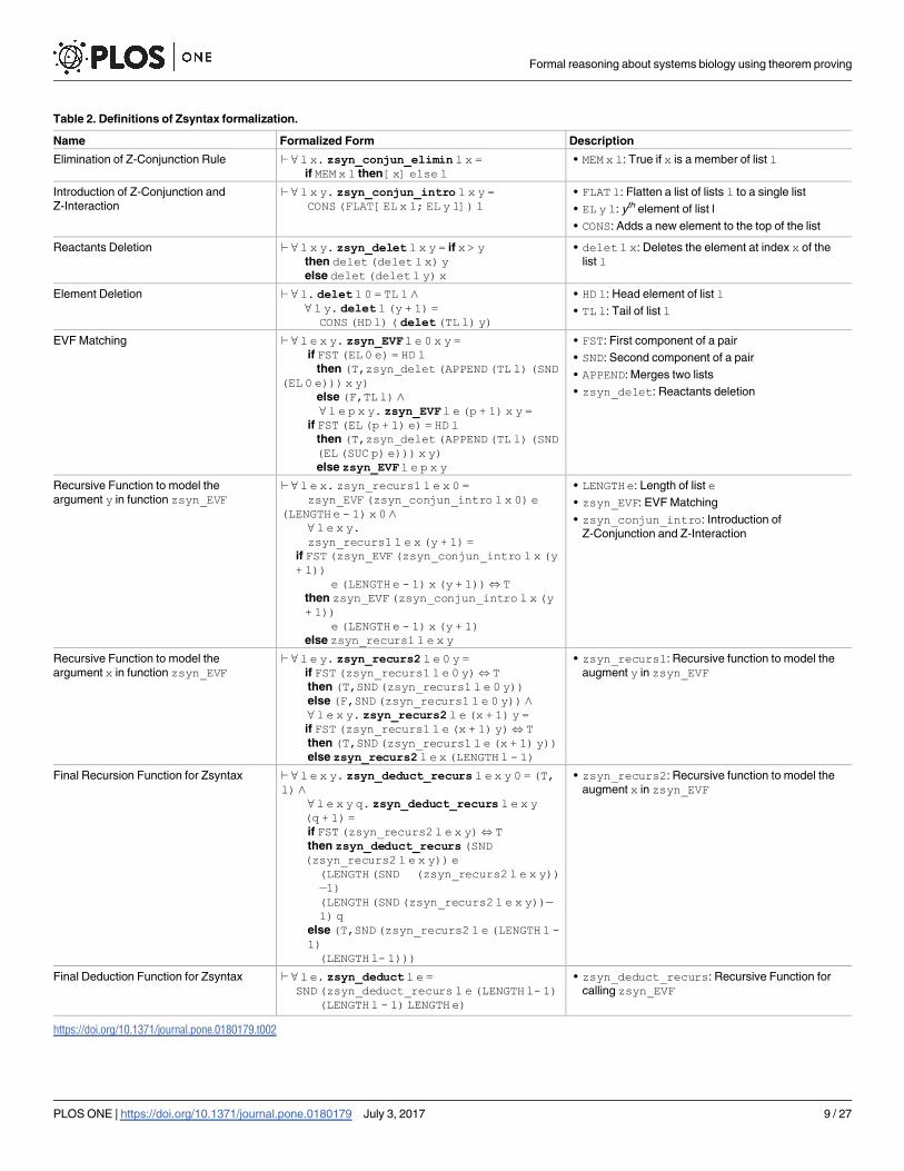
Table 2. Definitions of Zsyntax formalization.

Name Formalized Form Description

Elimination of Z-Conjunction Rule ‘ 8 l x. zsyn_conjun_elimin l x =if MEM x l then [x] else l

• MEM x l: True if x is a member of list l

Introduction of Z-Conjunction and

Z-Interaction

‘ 8 l x y. zsyn_conjun_intro l x y =CONS (FLAT [EL x l; EL y l]) l

• FLAT l: Flatten a list of lists l to a single list

• EL y l: yth element of list l

• CONS: Adds a new element to the top of the list

Reactants Deletion ‘ 8 l x y. zsyn_delet l x y = if x > ythen delet (delet l x) yelse delet (delet l y) x

• delet l x: Deletes the element at index x of the

list l

Element Deletion ‘ 8 l. delet l 0 = TL l ^8 l y. delet l (y + 1) =

CONS (HD l) ( delet (TL l) y)

• HD l: Head element of list l

• TL l: Tail of list l

EVF Matching ‘ 8 l e x y. zsyn_EVFl e 0 x y =if FST (EL 0 e) = HD l

then (T,zsyn_delet (APPEND(TL l) (SND(EL 0 e))) x y)

else (F,TL l) ^8 l e p x y. zsyn_EVFl e (p + 1) x y =

if FST (EL (p + 1) e) = HD lthen (T,zsyn_delet (APPEND(TL l) (SND(EL (SUC p) e))) x y)else zsyn_EVFl e p x y

• FST: First component of a pair

• SND: Second component of a pair

• APPEND: Merges two lists

• zsyn_delet: Reactants deletion

Recursive Function to model the

argument y in function zsyn_EVF‘ 8 l e x. zsyn_recurs1 l e x 0 =

zsyn_EVF (zsyn_conjun_intro l x 0) e(LENGTHe - 1) x 0 ^

8 l e x y.zsyn_recurs1 l e x (y + 1) =

if FST (zsyn_EVF (zsyn_conjun_intro l x (y+ 1))

e (LENGTHe - 1) x (y + 1)), Tthen zsyn_EVF(zsyn_conjun_intro l x (y+ 1))

e (LENGTHe - 1) x (y + 1)else zsyn_recurs1 l e x y

• LENGTHe: Length of list e

• zsyn_EVF: EVF Matching

• zsyn_conjun_intro: Introduction of

Z-Conjunction and Z-Interaction

Recursive Function to model the

argument x in function zsyn_EVF‘ 8 l e y. zsyn_recurs2 l e 0 y =

if FST (zsyn_recurs1 l e 0 y), Tthen (T,SND(zsyn_recurs1 l e 0 y))else (F,SND(zsyn_recurs1 l e 0 y)) ^8 l e x y. zsyn_recurs2 l e (x + 1) y =if FST (zsyn_recurs1 l e (x + 1) y), Tthen (T,SND(zsyn_recurs1 l e (x + 1) y))else zsyn_recurs2 l e x (LENGTHl - 1)

• zsyn_recurs1: Recursive function to model the

augment y in zsyn_EVF

Final Recursion Function for Zsyntax ‘ 8 l e x y. zsyn_deduct_recurs l e x y 0 = (T,l) ^

8 l e x y q. zsyn_deduct_recurs l e x y(q + 1) =if FST (zsyn_recurs2 l e x y), Tthen zsyn_deduct_recurs (SND(zsyn_recurs2 l e x y)) e

(LENGTH(SND (zsyn_recurs2 l e x y))—1)(LENGTH(SND (zsyn_recurs2 l e x y))—1) q

else (T,SND(zsyn_recurs2 l e (LENGTHl -1)(LENGTHl- 1)))

• zsyn_recurs2: Recursive function to model the

augment x in zsyn_EVF

Final Deduction Function for Zsyntax ‘ 8 l e. zsyn_deduct l e =SND (zsyn_deduct_recurs l e (LENGTHl- 1)

(LENGTHl - 1) LENGTH e)

• zsyn_deduct_recurs: Recursive Function for

calling zsyn_EVF






one. This whole process can be done using functions zsyn_recurs1 and zsyn_recurs2,

given in Table 2. In the function zsyn_recurs1, we first place the combination of molecules

indexed by variables x and y at the top of the list l using the introduction of Z-Conjunction

rule. Then, this modified list l is passed to the function zsyn_EVF, which is recursively called

by the function zsyn_recurs1. Moreover, we instantiate the variable p of the function

zsyn_EVFwith the length of the EVF list (LENGTHe - 1) so that every new combination

of the list l is compared with all the elements of the list of EVFs e. The function zsyn_re-curs1 terminates upon finding a match in the list of EVFs and returns true (T) as the first ele-

ment of its output pair, which acts as a flag for the status of this match. The second function

zsyn_recurs2 checks, if a match in the list of EVFs e is found (if the flag returns true (T))

then it terminates and returns the output list of the function zsyn_recurs1. Otherwise, it

recursively checks for the match with all of the remaining values of the variable x. In the case

of a match, these two functions zsyn_recurs1 and zsyn_recurs2have to be called all

over again with the new updated list. This iterative process continues until no match is found

in the execution of these functions. This overall behaviour can be expressed in HOL Light by

the recursive function zsyn_deduct_recurs, given in Table 2. In order to guarantee the

Fig 2. Graphical depiction of formalization of Zsyntax. (a) Elimination of the Z-Conjunction Rule (zsyn_conjun_elimin) (b) Introduction of

Z-Conjunction (zsyn_conjun_intro) (c) Reactants Deletion (zsyn_delet) (d) EVF Matching (zsyn_EVF).






correct operation of deduction, we instantiate the variable of recursion (q) with a value that is

greater than the total number of EVFs so that the application of none of the EVF is missed.

Similarly, in order to ensure that all the combinations of the list l are checked against the

entries of the EVF list e, the value LENGTH l - 1 is assigned to both of the variables x and y.

Thus, the final deduction function for Zsyntax can be modeled as the function zsyn_de-duct, given in Table 2. The function zsyn_deduct accepts the initial list of molecules land the list of valid EVFs e and returns a list of final outcomes of the experiment under the

given conditions. Next, in order to check, if the desired molecule is present in this list (the out-

put of the function zsyn_deduct), we apply the elimination of the Z-Conjunction rule pre-

sented as function zsyn_conjun_elimin, given in Table 2. More detail about the behavior

of all of these functions can be found in our proof script [63].

These formal definitions enable us to check recursively all of the possible combinations of

the molecules, present in the initial list l, against each of the first element of the list of EVFs e.

Upon finding a match, the reacting molecules are replaced by their outcome in the initial list

of molecules l by applying the corresponding EVF. This process is repeated on the current

updated list of molecules until there are no further molecules reacting with each other. The list

l at this point contains the post-reaction molecules. Finally, the elimination of the Z-Conjunc-

tion rule zsyn_conjun_elimin, given in Table 2, is applied to obtain the desired outcome

of the given biological experiment.

In order to prove the correctness of the formal definitions presented above, we verify a cou-

ple of key properties of Zsyntax involving operators depicting the vital behaviour of the molec-

ular reactions. The first verified property captures the scenario when there is no reacting

molecule present in the initial list of the experiment. As a result of this scenario, the post-

experiment molecules are the same as the pre-experiment molecules. The second property

deals with the case when there is only one set of reacting molecules in the given initial list of

molecules and in this scenario we verify that after the execution of the Zsyntax based experi-

ment, the list of post-experiment molecules contains the products of the reacting molecules

minus its reactant along with the remaining non-reacting molecules provided at the beginning

of the experiment. We formally specified both of these properties, representing the no reaction

and single reaction scenarios in higher-order logic using the formal definitions presented ear-

lier in this section. The formal verification results about these properties are given in Table 3

and more details can be found in the description of their formalization [18, 63]. The formaliza-

tion presented in this section provides an automated reasoning support for the Zsyntax based

molecular biological experiments within the sound core of HOL Light theorem prover.

Formalization of reaction kinetics

Reaction kinetics [64] is the study of rates at which biological processes interact with each

other and how the corresponding processes are affected by these reactions. The rate of a reac-

tion provides the information about the evolution of the concentration of the species (e.g.,

molecules) over time. A process is basically a chain of reactions, called pathway, and the inves-

tigation about the rate of a process implies the rate of these pathways. Generally, biological

reactions can be either irreversible (unidirectional) or reversible (bidirectional). We formally

define this fact by an inductive enumerating data-type reaction_type, given in Table 4.

In order to analyze a biological process, we need to know its kinetic reaction based model,

which comprises of a set of m species, X = {X1, X2, X3,. . ., Xm} and a set of n reactions, R = {R1,

R2, R3,. . ., Rn}. An irreversible reaction Rj, {1� j� n} can generally be written as:

Rj : s1;jX1 þ s2;jX2 þ . . .þ sm;jXm!kj

�s1;jX1 þ�s2;jX2 þ . . .þ�sm;jXm. Similarly, a reversible reaction

Rj, {1� j� n} can be described as:




Rj : s1;jX1 þ s2;jX2 þ . . .þ sm;jXm⇄kjr

kj f

�s1;jX1 þ�s2;jX2 þ . . .þ�sm;jXm. The coefficients

s1;j; s2;j; . . . ; sm;j;�s1;j;�s2;j; . . . ;�sm;j are the non-negative integers and represent the stoichiometries

of the species taking part in the reaction. The non-negative integer kj is the kinetic rate con-

stant of the irreversible reaction. The non-negative integers kjf

and kjr

are the forward and

reverse kinetic rate constants of the reversible reaction, respectively [65]. In a biological reac-

tion, we model a biological entity as a pair (N,R), where the first element represents the stoi-

chiometry and the second element is the concentration of the molecule. We formally model a

biological reaction as the type abbreviation bio_reaction [63], given in Table 4.

The dynamic behavior of the biological systems is described by a set of ordinary differential

equations (ODEs) and the evolution of the system is captured by analyzing the change in the

concentration of the species (i.e., time derivatives):d½Xi �dt ¼

Pnj¼1

ni;jvj, where ni, j is the stoichio-

metric coefficient of the molecular species Xi in reaction Rj (i.e., ni;j ¼ �si;j � si;j). The parameter

vj represents the flux of the reaction Rj, which can be computed by the law of mass action [14],

Table 3. Formal verification of Zsyntax properties.


Case:1 No

Reaction

‘ 8 e l.A1:*(NULL e) Â2:*(NULL l) Â3: (8 a x y. MEM a e ^

x < LENGTH l ^ y < LENGTH l)*MEM (FST a)[HD (zsyn_conjun_intro l xy)])

) zsyn_deduct l e = l

• e: List of EVFs

• l: List of molecules

• A1: List e is non-empty

• A2: List l is non-empty

• A3: The formalization of the no-reaction-possibility condition

• Conclusion: Both the pre and post-experiment lists of molecules are the same

Case:2 Single

Reaction

‘ 8 e l z x’ y’.A1:*(NULL e) Â2:*(NULL (SND (EL z e))) Â3: 1 < LENGTH l Â4: x’ 6¼ y’ Â5: x’ < LENGTHl Â6: y’ < LENGTHl Â7: z < LENGTH e Â8: ALL_DISTINCT (APPENDl

(SND (EL z e)))Â9: (8 a b. a 6¼ b

) FST (EL a e) 6¼ FST (EL be)) ^

A10: (8 k x y. x < LENGTHk ^y < LENGTHk ^

(8 j. MEM j k) MEM j l _(9 q. MEM q e ^ MEM j (SND q)))if (EL x k = EL x’ l) ^ (EL y k = ELy’ l)then HD (zsyn_conjun_introk x y) =

FST (EL z e)else 8 a. MEM a e) FST a 6¼ HD

(zsyn_conjun_intro k x y))) zsyn_deduct l e

= zsyn_delet (APPENDl (SND(EL z e))) x’ y’

• e: List of EVFs

• l: List of molecules

• A1-A2: The list e and the second element of the pair at index z of the list e is non-empty

• A3: List l, i.e., the list of initial molecules, contains at least two elements

• A4: The indices x’ and y’ are distinct

• A5-A7: The indices x’, y’ and z fall within the range of elements of their respective lists

of molecules l or EVFs e

• A8: All elements of the list l and the resulting molecules of the EVF at index z are distinct

• A9: All first elements of the pairs in list e are distinct

• A10: It models the scenario where there is only one pair of reactants present in the

reaction

• Conclusion: The scenario when the resulting element, available at the location z of the

EVF list, is appended to the list of molecules while the elements available at the indices

x’ and y’ of l are removed during the execution of the function zsyn_deduct on the

given lists l and e






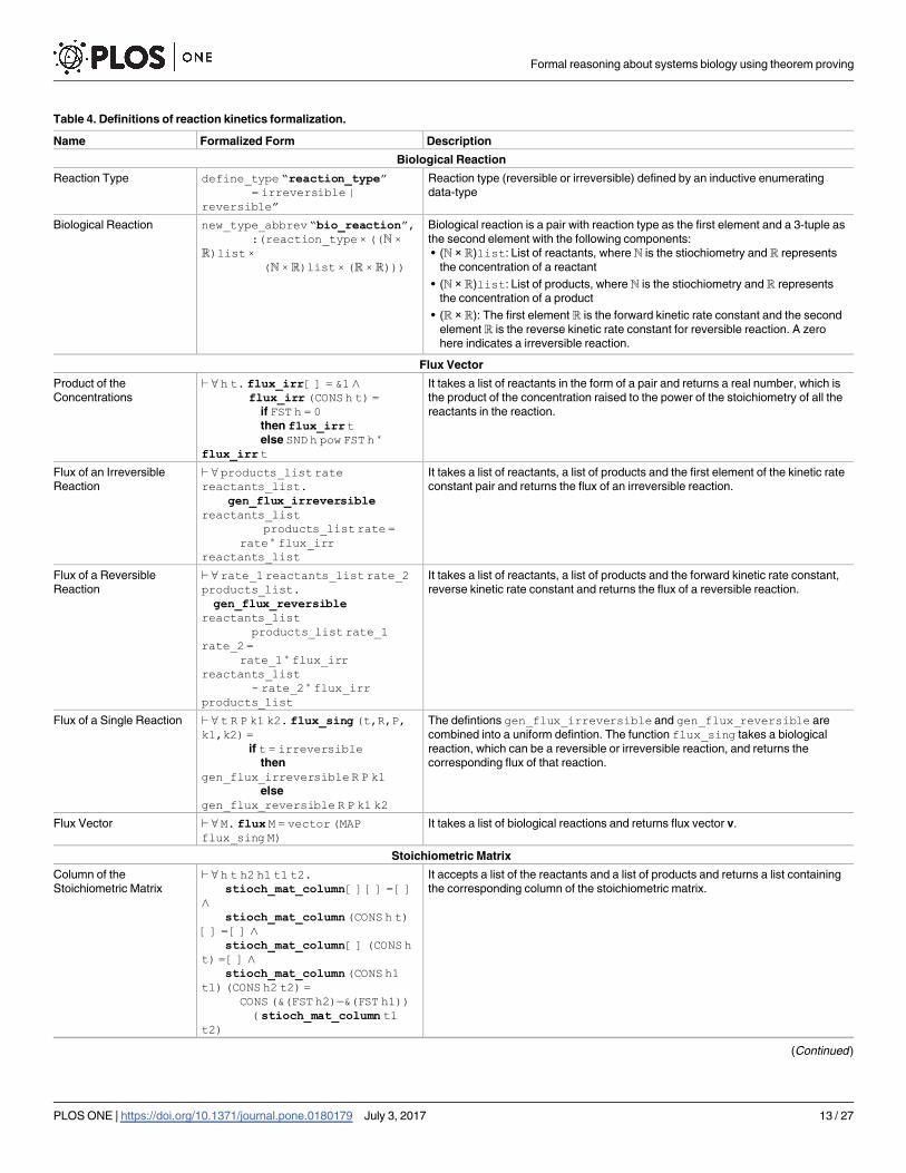
Table 4. Definitions of reaction kinetics formalization.


Biological Reaction

Reaction Type define_type “reaction_type”= irreversible |

reversible”

Reaction type (reversible or irreversible) defined by an inductive enumerating

data-type

Biological Reaction new_type_abbrev“bio_reaction”,:(reaction_type× ((N ×

R)list ×(N × R)list × (R × R)))

Biological reaction is a pair with reaction type as the first element and a 3-tuple as

the second element with the following components:

• (N × R)list: List of reactants, where N is the stiochiometry and R represents

the concentration of a reactant

• (N × R)list: List of products, where N is the stiochiometry and R represents

the concentration of a product

• (R × R): The first element R is the forward kinetic rate constant and the second

element R is the reverse kinetic rate constant for reversible reaction. A zero

here indicates a irreversible reaction.

Flux Vector

Product of the

Concentrations

‘ 8 h t. flux_irr[ ] = &1 ^flux_irr (CONS h t) =

if FST h = 0then flux_irrtelse SND h pow FST h �

flux_irrt

It takes a list of reactants in the form of a pair and returns a real number, which is

the product of the concentration raised to the power of the stoichiometry of all the

reactants in the reaction.

Flux of an Irreversible

Reaction

‘ 8 products_list ratereactants_list.

gen_flux_irreversiblereactants_list

products_list rate =rate � flux_irr

reactants_list

It takes a list of reactants, a list of products and the first element of the kinetic rate

constant pair and returns the flux of an irreversible reaction.

Flux of a Reversible

Reaction

‘ 8 rate_1reactants_list rate_2products_list.gen_flux_reversible

reactants_listproducts_list rate_1

rate_2 =rate_1 � flux_irr

reactants_list- rate_2 � flux_irr

products_list

It takes a list of reactants, a list of products and the forward kinetic rate constant,

reverse kinetic rate constant and returns the flux of a reversible reaction.

Flux of a Single Reaction ‘ 8 t R P k1 k2. flux_sing (t,R,P,k1,k2) =

if t = irreversiblethen

gen_flux_irreversible R P k1else

gen_flux_reversible R P k1 k2

The defintions gen_flux_irreversible and gen_flux_reversible are

combined into a uniform defintion. The function flux_sing takes a biological

reaction, which can be a reversible or irreversible reaction, and returns the

corresponding flux of that reaction.

Flux Vector ‘ 8 M. flux M = vector(MAPflux_sing M)

It takes a list of biological reactions and returns flux vector v.

Stoichiometric Matrix

Column of the


‘ 8 h t h2 h1 t1 t2.stioch_mat_column[ ] [ ] = [ ]

^

stioch_mat_column(CONS h t)[ ] = [ ] ^

stioch_mat_column[ ] (CONS ht) = [ ] ^

stioch_mat_column(CONS h1t1) (CONS h2 t2) =

CONS (&(FST h2)—&(FST h1))( stioch_mat_column t1

t2)

It accepts a list of the reactants and a list of products and returns a list containing

the corresponding column of the stoichiometric matrix.

(Continued )




i.e., the rate (also called flux) of a reaction is proportional to the concentration of the

reactant (c) raised to the power of its stoichiometry (s), i.e., cs. We define the function

gen_flux_irreversible,given in Table 4, to obtain the flux of an irreversible

reaction [63].

A reversible reaction can be divided into two irreversible reactions with the forward kinetic

rate constant and the reverse kinetic rate constant, respectively. The rate/flux of a reversible

reaction is obtained by taking the differences of the fluxes of the two irreversible reactions. We

formally define the flux of a reversible reaction by the function gen_flux_reversible,

given in Table 4. Next, we combine the functions gen_flux_irreversibleand

gen_flux_reversible into one uniform function flux_single (Table 4)[63] to

obtain the flux of a single reaction.

For all reactions from 1 to n of a biological system, the flux becomes a flux vector as v = (v1,

v2,. . ., vn)T and the system of ODEs can be written in the vectorial form as:d½X�dt ¼ Nv, where

[X] = (X1 X2,. . ., Xn)T is a vector of the concentration of all of the species participating in the

reaction and N is the stoichiometric matrix of order m × n. We can obtain the flux vector v for

a chain of reactions of a biological system by the function flux [63], given in Table 4.

Next, we formalize the notion of stoichiometric matrix N by the function st_matrix [63]

given in Table 4. Finally, in order to formalize the left-hand side of above vector equation, i.e.,d½X�dt , we define a function entities_deriv_vecwhich takes a list containing the concen-

trations of all species and returns a vector with each element represented in the form of a real-

valued derivative.

We can utilize this infrastructure to model arbitrary biological networks consisting of any

number of reactions. For example, a biological network consisting of a list of E biological spe-

cies and M biological reactions can be formally represented by the following general kinetic

model:

ððentitiesderivvec E tÞ : real^mÞ ¼ transpððstmatrix MÞ : real^m^nÞ � � flux M

We used the formalization of the reaction kinetics to verify some generic properties of bio-

logical reactions, such as irreversible consecutive reactions, reversible and irreversible mixed

Table 4. (Continued)


Vector of the


Column

‘ 8 t k1 k2 R P.st_matrix_sing (t,R,P,k1,k2)

= vector(stioch_mat_column R P)

It takes a single biological reaction (bio_reaction) and returns a vector (Rm), which

corresponds to the column of the stoichiometric matrix.

Stoichiometric Matrix ‘ 8 M. st_matrix M= vector (MAP

st_matrix_sing M)

It takes a list of biological reactions and returns a stiochiometric matrix (in

transposed form) using the MAP function, which applies the function

st_matrix_sing on every element of the list M.

Vector of Derivative

Derivative of a List of

Functions

‘ 8 h t x. map_real_deriv [ ] x = [ ]^

map_real_deriv (CONS h t) x =APPEND[real_derivativeh x]

( map_real_deriv t x)

It takes a list containing the concentrations of all the species taking part in the

reaction and maps a real derivative over each function of the list using the function

real_derivative, which represents the real-valued derivative of a function

Derivative of a Vector ‘ 8 L t. entities_deriv_vec L t= vector (map_real_derivL

t)

It accepts a list containing the concentrations of species and returns a vector with

each element represented in the form of a real-valued derivative, which is left-

hand side of vector equation, i.e.,d½X�dt .






reactions. The main idea is to express the given biological network as a kinetic model and ver-

ify that the given solution (mathematical expression) of each biological entity satisfies the

resulting set of coupled differential equations. This verification is quite important as such

expressions are used to predict the outcomes of various drugs and to understand the time evo-

lution of different molecules in the reactions of the biological systems.

The irreversible consecutive reactions. We consider a general irreversible consecutive

reaction scheme as shown in Fig 3a. In the first reaction, A is the reactant and B is the product

whereas k1 represents the kinetic rate constant of the reaction. Similarly, in the second reac-

tion, B is the reactant, C is the product and k2 is its kinetic rate constant. We formally model

this reaction scheme as a HOL Light function rea_sch_01, given in Table 5, and the formal-

ization details are available as a technical report [66]. We moreover verify the solution of its

kinetic model in HOL Light. The formal verification results are given in Table 6 [63].

Fig 3. Reaction schemes. (a) Irreversible Consecutive Reactions (b) Consecutive Reactions with the Second Step being Reversible (c)

Consecutive Reactions with the First Step as a Reversible Reaction (d) Consecutive Reactions with a Reversible Step.






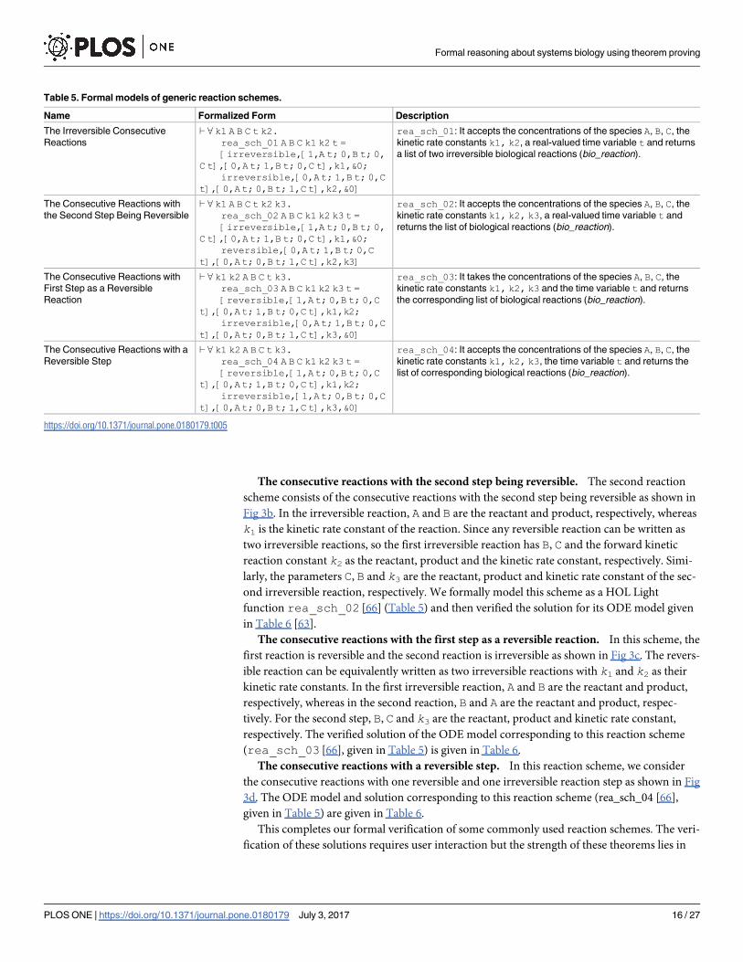
The consecutive reactions with the second step being reversible. The second reaction

scheme consists of the consecutive reactions with the second step being reversible as shown in

Fig 3b. In the irreversible reaction, A and B are the reactant and product, respectively, whereas

k1 is the kinetic rate constant of the reaction. Since any reversible reaction can be written as

two irreversible reactions, so the first irreversible reaction has B, C and the forward kinetic

reaction constant k2 as the reactant, product and the kinetic rate constant, respectively. Simi-

larly, the parameters C, B and k3 are the reactant, product and kinetic rate constant of the sec-

ond irreversible reaction, respectively. We formally model this scheme as a HOL Light

function rea_sch_02 [66] (Table 5) and then verified the solution for its ODE model given

in Table 6 [63].

The consecutive reactions with the first step as a reversible reaction. In this scheme, the

first reaction is reversible and the second reaction is irreversible as shown in Fig 3c. The revers-

ible reaction can be equivalently written as two irreversible reactions with k1 and k2 as their

kinetic rate constants. In the first irreversible reaction, A and B are the reactant and product,

respectively, whereas in the second reaction, B and A are the reactant and product, respec-

tively. For the second step, B, C and k3 are the reactant, product and kinetic rate constant,

respectively. The verified solution of the ODE model corresponding to this reaction scheme

(rea_sch_03 [66], given in Table 5) is given in Table 6.

The consecutive reactions with a reversible step. In this reaction scheme, we consider

the consecutive reactions with one reversible and one irreversible reaction step as shown in Fig

3d. The ODE model and solution corresponding to this reaction scheme (rea_sch_04 [66],

given in Table 5) are given in Table 6.

This completes our formal verification of some commonly used reaction schemes. The veri-

fication of these solutions requires user interaction but the strength of these theorems lies in

Table 5. Formal models of generic reaction schemes.


The Irreversible Consecutive

Reactions

‘ 8 k1 A B C t k2.rea_sch_01 A B C k1 k2 t =[irreversible,[1,A t; 0,B t; 0,

C t],[0,At; 1,B t; 0,C t],k1,&0;irreversible,[0,At; 1,B t; 0,C

t],[0,At; 0,B t; 1,C t],k2,&0]

rea_sch_01: It accepts the concentrations of the species A, B, C, the

kinetic rate constants k1, k2, a real-valued time variable t and returns

a list of two irreversible biological reactions (bio_reaction).

The Consecutive Reactions with

the Second Step Being Reversible

‘ 8 k1 A B C t k2 k3.rea_sch_02 A B C k1 k2 k3 t =[irreversible,[1,A t; 0,B t; 0,

C t],[0,At; 1,B t; 0,C t],k1,&0;reversible,[0,At; 1,B t; 0,C

t],[0,At; 0,B t; 1,C t],k2,k3]


kinetic rate constants k1, k2, k3, a real-valued time variable t and

returns the list of biological reactions (bio_reaction).

The Consecutive Reactions with

First Step as a Reversible

Reaction

‘ 8 k1 k2 A B C t k3.rea_sch_03 A B C k1 k2 k3 t =[reversible,[1,At; 0,B t; 0,C

t],[0,At; 1,B t; 0,C t],k1,k2;irreversible,[0,At; 1,B t; 0,C

t],[0,At; 0,B t; 1,C t],k3,&0]

rea_sch_03: It takes the concentrations of the species A, B, C, the

kinetic rate constants k1, k2, k3 and the time variable t and returns

the corresponding list of biological reactions (bio_reaction).

The Consecutive Reactions with a

Reversible Step

‘ 8 k1 k2 A B C t k3.rea_sch_04 A B C k1 k2 k3 t =[reversible,[1,At; 0,B t; 0,C

t],[0,At; 1,B t; 0,C t],k1,k2;irreversible,[1,At; 0,B t; 0,C

t],[0,At; 0,B t; 1,C t],k3,&0]


kinetic rate constants k1, k2, k3, the time variable t and returns the

list of corresponding biological reactions (bio_reaction).






Table 6. Formal verification of reaction kinetics properties.


The Irreversible

Consecutive Reactions

‘ 8 A B C t k1 k2.A1: 0 < k1 ^ A2: 0 < k2 ^ A3: (k2 −k1 6¼0) Â4: A(0) = A0 ^ A5: B(0) = 0 ^ A6: C(0) = 0 Â7: 8t. A(t) = A0 e

(−k1 t) ^

A8: 8t: BðtÞ ¼ A0

k1

ðk2 � k1Þðe� k1t � e� k2tÞ ^

A9: 8t: CðtÞ ¼ A0 1 �k2

ðk2 � k1Þe� k1t �

k1

ðk1 � k2Þe� k2t

� �

) entities_deriv_vec[A; B; C] t =transp (st_matrix(rea_sch_01A B C k1 k2 t)) ��

flux (rea_sch_01A B C k1 k2 t)

• ��: Matrix-vector multiplication

• rea_sch_01: Formal model of the given reaction

scheme

• transp: Transpose of a matrix

• A1-A2: The kinetic rate constants of all the reactions are

non-negative.

• A3: The denominators of the expressions of B t and C tare not zero in order to avoid singularities

• A4-A6: These are the initial concentrations of the

species

• A7-A9: The concentrations of the species A, B and C at

any time t (solutions of the ODE model)

• Conclusion: It describes the ODE model (Vector

Equation) for the given reaction scheme

The Consecutive Reactions

with the Second Step being

Reversible

‘ 8 A B C t k1 k2 k3.A1: 0 < k1 ^ A2: 0 < k2 ^ A3: 0 < k3 Â4: A(0) = A0 ^ A5: B(0) = 0 ^ A6: C(0) = 0 Â7: r1 = k1 ^ A8: r2 = k2 +k3 ^ A9: r1 6¼r2 Â10: 8t. A(t) = A0 e

(−k1 t) ^

A11: 8t: BðtÞ ¼ k1A0

k3

r1r2þ

r2 � k3

r1ðr1 � r2Þe� r2t þ

k3 � r1

r1ðr1 � r2Þe� r1t

� �^

A12: 8t: CðtÞ ¼

k1k2A01

r1r2þ 1

r1ðr1 � r2Þe� r1t þ 1


� �^

) entities_deriv_vec[A; B; C] t =transp (st_matrix(rea_sch_02A B C k1 k2 k3 t)) ��

flux (rea_sch_02A B C k1 k2 k3 t)


scheme


non-negative.


species

• A7-A8: These are introduced to simplify the expressions

for the concentrations of the species

• A9: It, along with the first three assumptions (A1-A3),

ensures that the denominators of the expressions for B tand C t are not zero in order to avoid singularities

• A10-A12: The concentrations of the species A, B and Cat any time t (solutions of the ODE model)

• Conclusion: It describes the ODE model for the given

reaction scheme


with the First Step being

Reversible

‘ 8 A B C t k1 k2 k3.A1: 0 < k1 ^ A2: 0 < k2 ^ A3: 0 < k3 Â4: A(0) = A0 ^ A5: B(0) = 0 ^ A6: C(0) = 0 Â7: r1 r2 = k1 k3 ^ A8: r1 +r2 = k1 +k2 +k3 Â9: r1 6¼0 ^ A10: r2 6¼0 ^ A11: r1 6¼r2 Â12: 8t: AðtÞ ¼

A0

r2 � r1ðk2 þ k3 � r1Þe

ð� r1tÞ � ðk2 þk3 � r2Þeð� r2tÞð Þ ^

A13: 8t: BðtÞ ¼A0k1

r2 � r1e� r1t � e� r2tð Þ ^

A14: 8t: CðtÞ ¼ A0 1þk1k3


k1k3


� �^




scheme


non-negative.


species



• A9-A11: The denominators of the expressions of A t, Bt and C t are not zero in order to avoid singularities



reaction scheme


with a Reversible Step

‘ 8 A B C t k1 k2 k3.A1: 0 < k1 ^ A2: 0 < k2 ^ A3: 0 < k3 Â4: A(0) = A0 ^ A5: B(0) = 0 ^ A6: C(0) = 0 Â7: r1 r2 = k2 k3 ^ A8: r1 +r2 = k1 +k2 +k3 Â9: r1 6¼0 ^ A10: r2 6¼0 ^ A11: r1 6¼r2 ^

A12: 8t: AðtÞ ¼ A0

k2 � r1

r2 � r1e� r1t �

k2 � r2

r2 � r1e� r2t

� �^

A13: 8t: BðtÞ ¼k1A0

r2 � r1e� r1t � e� r2tð Þ ^

A14: 8t: CðtÞ ¼ A0 1þk3ðk2 � r1Þ


k3ðk2 � r2Þ


� �^




scheme


non-negative.


species



• A9-A11: The denominators of the expressions of A t, Bt and C t are not zero in order to avoid singularities



reaction scheme






the fact that they have been verified for arbitrary values of parameters, such as k1 and k2, etc.

This is a unique feature of higher-order-logic theorem proving that is not possible in the case

of simulation where such continuous expressions are tested for few samples of such parame-

ters. Another important aspect is the explicit presence of all assumptions required to verify the

set of ODEs. For example, such assumptions for the above-mentioned reaction schemes are

not mentioned in Korobov et al.’s paper [67]. More details about the formalization of all above-

mentioned types and functions and the formal verification of all above properties, and its

source code can be found on our project’s webpage [63].

Case studies

In this section, we use our proposed framework to formally reason about three case studies: In

the first, we formally analyse the reaction involving the phosphorylation of TP53 using our for-

malization of Zsyntax. In the second, we formally derive the time evolution expressions of dif-

ferent tumor cell types, which are used to predict the tumor population and volume at a given

time instant, using our formalization of reaction kinetics. In the third, we take another model

for the growth of tumor cells and perform both the Zsyntax and reaction kinetic based formal

analysis using our proposed formalizations presented in the Result section of the paper.

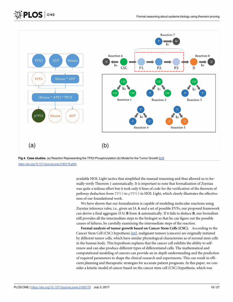
TP53 phosphorylation. TP53 gene encodes p53 protein, which plays a crucial role in reg-

ulating the cell cycle of multicellular organisms and works as a tumour suppressor for prevent-

ing cancer [13]. The pathway leading to TP53 phosphorylation (p(TP53)) is shown in Fig 4a.

The green-colored circle represents the desired product, whereas, the blued-colored circles

describe the chemical interactions in the pathway. Similarly, each rectangle in Fig 4a contains

the total number of molecules at a given time. It can be clearly seen from the figure that when-

ever a biological reaction results into a product, the reactants get consumed, which satisfies the

stoichiometry of a reaction. Now, we present the formal verification of pathway deduction

from TP53 to p(TP53) using our formalization of Zsyntax, presented in the last section.

In classical Zsyntax format, the reaction of the pathway leading from TP53 to p(TP53) [13]

can be represented by a theorem as TP53 & ATP & Kinase ‘ p(TP53). Based on our for-

malization, it can be defined as follows:

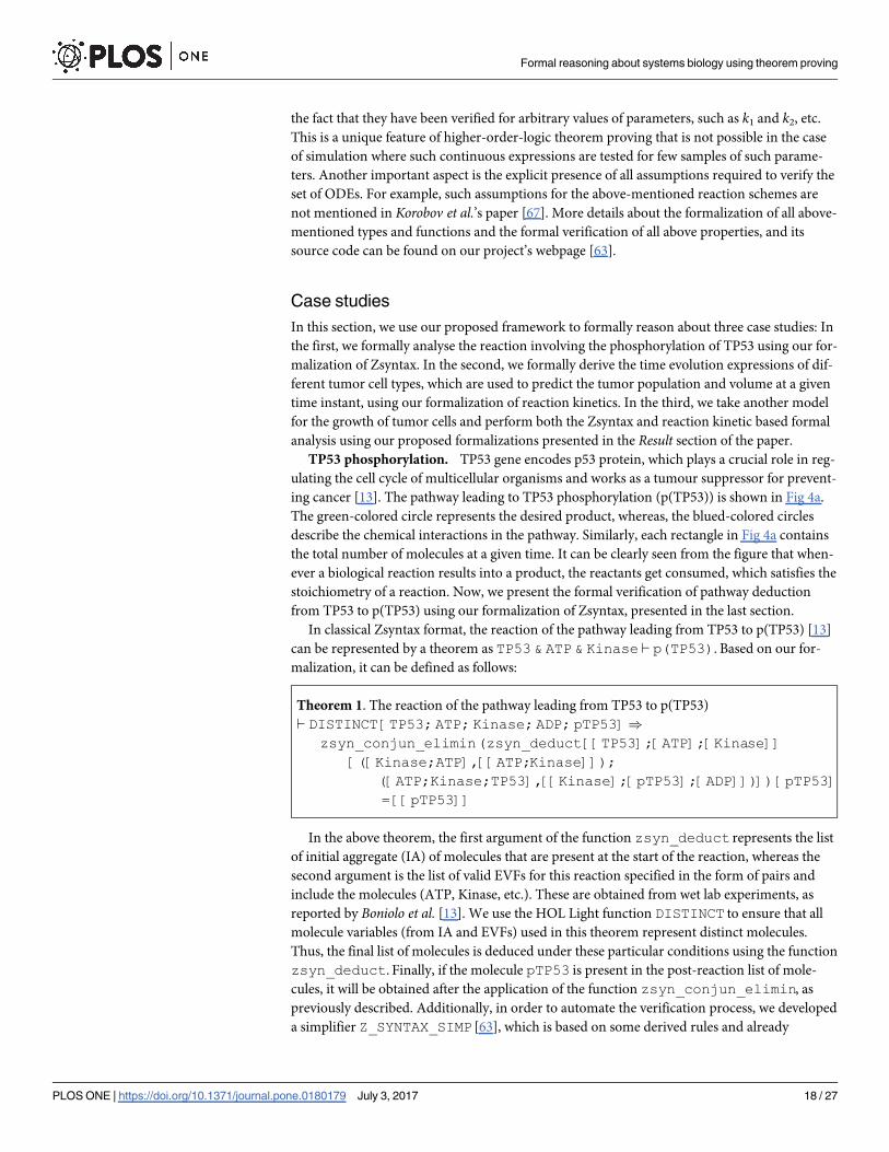
Theorem 1. The reaction of the pathway leading from TP53 to p(TP53)

‘ DISTINCT[TP53; ATP; Kinase;ADP; pTP53])zsyn_conjun_elimin(zsyn_deduct[[TP53];[ATP];[Kinase]]

[([Kinase;ATP],[[ATP;Kinase]]);([ATP;Kinase;TP53],[[Kinase];[pTP53];[ADP]])]) [pTP53]= [[pTP53]]

In the above theorem, the first argument of the function zsyn_deduct represents the list

of initial aggregate (IA) of molecules that are present at the start of the reaction, whereas the

second argument is the list of valid EVFs for this reaction specified in the form of pairs and

include the molecules (ATP, Kinase, etc.). These are obtained from wet lab experiments, as

reported by Boniolo et al. [13]. We use the HOL Light function DISTINCT to ensure that all

molecule variables (from IA and EVFs) used in this theorem represent distinct molecules.

Thus, the final list of molecules is deduced under these particular conditions using the function

zsyn_deduct. Finally, if the molecule pTP53 is present in the post-reaction list of mole-

cules, it will be obtained after the application of the function zsyn_conjun_elimin, as

previously described. Additionally, in order to automate the verification process, we developed

a simplifier Z_SYNTAX_SIMP [63], which is based on some derived rules and already




available HOL Light tactics that simplified the manual reasoning and thus allowed us to for-

mally verify Theorem 1 automatically. It is important to note that formalization of Zsyntax

was quite a tedious effort but it took only 6 lines of code for the verification of the theorem of

pathway deduction from TP53 to pTP53 in HOL Light, which clearly illustrates the effective-

ness of our foundational work.

We have shown that our formalization is capable of modeling molecular reactions using

Zsyntax inference rules, i.e., given an IA A and a set of possible EVFs, our proposed framework

can derive a final aggregate (FA) B from A automatically. If it fails to deduce B, our formalism

still provides all the intermediate steps to the biologist so that he can figure out the possible

causes of failures, by carefully examining the intermediate steps of the reaction.

Formal analysis of tumor growth based on Cancer Stem Cells (CSC). According to the

Cancer Stem Cell (CSC) hypothesis [68], malignant tumors (cancers) are originally initiated

by different tumor cells, which have similar physiological characterises as of normal stem cells

in the human body. This hypothesis explains that the cancer cell exhibits the ability to self-

renew and can also produce different types of differentiated cells. The mathematical and

computational modeling of cancers can provide an in-depth understanding and the prediction

of required parameters to shape the clinical research and experiments. This can result in effi-

cient planning and therapeutic strategies for accurate patient prognosis. In this paper, we con-

sider a kinetic model of cancer based on the cancer stem cell (CSC) hypothesis, which was

Fig 4. Case studies. (a) Reaction Representing the TP53 Phosphorylation (b) Model for the Tumor Growth [20].






recently proposed in Molina-Pena et al.’s paper [20]. In this model, four types of events are

considered: 1) CSC self-renewal; 2) maturation of CSCs into P cells; 3) differentiation to D

cells; and 4) death of all cell subtypes. All of these types of reactions are driven by different rate

constants as shown in Fig 4b.

In the following, we provide the possible reactions in the considered model of cancer [20]:

1. Expansion of CSCs can be accomplished through symmetric division, where one CSC can

produce two CSCs, i.e., CSC!k12CSC.

2. A CSC can undergo asymmetric division (whereby one CSC gives rise to another CSC and

a more differentiated progenitor (P) cell). This P cell possesses intermediate properties

between CSCs and differentiated (D) cells, i.e., CSC!k2 CSCþ P.

3. The CSCs can also differentiate to P cells by symmetric division, i.e., CSC!k32P.

4. The P cells can either self-renew, with a decreased capacity compared to CSCs, or they can

differentiate to D cells, i.e., P!k42P, P!k5

2D.

5. All cellular subtypes can undergo cell death (M), i.e., CSC!k6 M, P!k7 M, D!k8 M.

In order to reduce the complexity of the resulting model, only three subtypes of cells are

considered: CSCs, transit amplifying progenitor cells (P), and terminally differentiated cells

(D) as shown in Fig 4b. This assumption is consistent with several experimental reports [20].

Our main objective is to derive the mathematical expressions, which characterize the time evo-

lution of CSC, P and D. Concretely, the values of these cells should satisfy the set of differential

equations that arise in the kinetic model of the proposed tumor growth. Once the expressions

of all cell types are known, the total number of tumor cells (N) in the human body can be com-

puted by the formula N(t) = CSC(t) + P(t) + D(t). Furthermore, the tumor volume (V) can be

calculated by the formula V(t) = 4.18 × 106 N(t), considering that the effective volume contri-

bution of a spherically shaped cell in a spherical tumor (i.e., 4.18 × 10−6 mm3/cell).We formally model the tumor growth model and verify the time evolution expressions for

CSC, P and D that satisfy the general kinetic model. We formally represent this requirement in

the following important theorem:

Theorem 2. Time Evolution Verification of Tumor Growth Model

‘ 8 k1 k2 k3 k4 k5 k6 k7 CSC P D M t k8.

A1: ((−k1 +k3 +k4 −k5 +k6 −k7 )(−k1 +k3 +k6 −k8 )(−k4 +k5 +k7 −k8 )6¼0)^A2: (k1 −k3 −k4 +k5 −k6 +k7 6¼0) ^A3: 8t. CSC(t) = e(k1 −k3 −k6 ) ^

A4:8t: PðtÞ ¼½ðeðk1 � k3 � k6Þt� eðk4 � k5 � k7ÞtÞðk2þ2k3Þ�

ðk1� k3� k4þk5� k6þk7Þ^

A5:8t: DðtÞ ¼ð2e� k8tðk2þ2k3Þk5½ð� 1þeðk4 � k5 � k7þk8ÞtÞk1þk3þk4� k5þk6� k7�

ð� k1þk3þk4� k5þk6� k7Þð� k1þk3þk6� k8Þð� k4þk5þk7� k8Þþ

ð2e� k8tðk2þ2k3Þk5½eðk1 � k3 � k6þk8Þtð� k4þk5þk7� k8Þþeðk4 � k5 � k7þk8Þtð� k3� k6þk8Þ�

ð� k1þk3þk4� k5þk6� k7Þð� k1þk3þk6� k8Þð� k4þk5þk7� k8Þ^

A6: real_derivativeM(t) = k6 CSC(t) + k7 P(t) + k8 D(t)) entities_deriv_vec[CSC; P; D; M] t =transp(st_matrix(tumor_growth_model CSC P D M k1 k2 k3 k4 k5k6 k7 k8 t))

��flux (tumor_growth_modelCSC P D M k1 k2 k3 k4 k5 k6 k7 k8 t))




where the first two assumptions (A1-A2) ensure that the time evolution expressions of Pand D do not contain any singularity (i.e., the value at the expression becomes undefined). The

next three assumptions (A3-A5) provide the time evolution expressions for CSC, P and D,

respectively. The last assumption (A6) is provided to discharge the subgoal characterizing the

time-evolution of M (dead cells), which is of no interest and does not impact the overall analysis

as confirmed by experimental evidences [20]. Finally, the conclusion of Theorem 2 is the

equivalent reaction kinetic (ODE) model of the CSC based tumor growth model. To facilitate

the verification process of the above theorem, we developed a simplifier, called KINETICSIMP, which sufficiently reduces the manual reasoning interaction with the theorem prover.

After the application of this simplifier, it only takes some arithmetic reasoning to conclude the

proof of Theorem 2. More details about the verification process can be found on our project’s

webpage [63].

The formal verification of the time-evolution of tumor cell types CSC, P and D in Theorem

2 can be easily used to formally derive the total population and volume of tumor cells. The

derived time-evolution expression, verified in Theorem 2, can also be used to understand how

the overall tumor growth model works. Moreover, potential drugs are usually designed using

the variation of the kinetic rate constants, such as k1, k2� � �k8 in Theorem 2, to achieve the

desired behavior of the overall tumor growth model and thus Theorem 2 can be utilized to

study this behavior formally. On similar lines, the variation of these parameters is used to plan

efficient therapeutic strategies for cancer patients and thus the formally verified result of Theo-

rem 2 can aid in accurately performing this task.

Combined Zsyntax and Reaction kinetic based formal analysis of the tumor growth

model. In this section, we consider another model for the growth of tumor cells and formally

analyze it using both of our Zsyntax and Reaction kinetics formalizations, presented in the

Results section of the paper.

Pathway Leading to Death of CSC

The pathway leading to death of CSC is shown in Fig 5a. The green-colored circle repre-

sents the desired product, whereas, the blued-colored circles describe the chemical interactions

in the pathway. We use our formalization of Zsyntax to deduce this pathway. In the classical

Zsyntax format, the reaction of the pathway leading from CSC to its death can be represented

by a theorem as CSC & P ‘ M. Based on our formalization, it can be defined as follows:

Fig 5. Case studies. (a) Reaction Representing the death of CSC (b) Another Model for the Growth of Tumor

Cell.






Theorem 3. The Reaction of the Pathway Leading from CSC to its Death (M)

‘ DISTINCT[CSC; P; M])zsyn_conjun_elimin(zsyn_deduct[[CSC];[P]][([CSC],[[CSC;P]]);([CSC;P],[[M]])])[M] = [[M]]

In the above theorem, the first argument of the function zsyn_deduct represents the list

of IA of molecules that are present at the start of the reaction, whereas the second argument is

the list of valid EVFs for this reaction specified in the form of pairs and include the molecules

(CSC, P, etc.). We use the HOL Light function DISTINCT to ensure that all molecule variables

(from IA and EVFs) used in this theorem represent distinct molecules. Thus, the final list of

molecules is deduced under these particular conditions using the function zsyn_deduct.

Finally, if the molecule M is present in the post-reaction list of molecules, it will be obtained

after the application of the function zsyn_conjun_elimin. We use the simplifier Z_SYN-TAX_SIMP [63] to formally verify Theorem 3 automatically.

Reaction Kinetic based Formal Analysis of a Tumor Growth based on CSC

We perform the reaction kinetic based formal analysis of a tumor growth model, which is

shown in Fig 5b. In this model, two types of events are considered: 1) maturation of CSCs into

P cells; 2) death of all cell subtypes. All of these types of reactions are driven by different rate

constants as shown in Fig 5b.

In the following, we provide the possible reactions in the considered tumor growth model:

1. A CSC can undergo asymmetric division (whereby one CSC gives rise to another CSC and

a more differentiated P cell), i.e., CSC!k1 CSCþ P.

2. All cellular subtypes can undergo cell death (M), i.e., CSC!k2 M, P!k3 M.

In order to reduce the complexity of the resulting model, only two subtypes of cells are con-

sidered: CSCs and transit amplifying progenitor cells (P) as shown in Fig 5b. Our main objec-

tive is to derive the mathematical expressions, which characterize the time evolution of CSC

and P. Concretely, the values of these cells should satisfy the set of differential equations that

arise in the kinetic model of the proposed tumor growth. Once the expressions of all cell types

are known, the total number of tumor cells (N) in the human body can be computed by the

formula N(t) = CSC(t) + P(t). We formalize the reaction kinetic based tumor growth model

and verify the time evolution expressions for CSC and P that satisfy the general kinetic model.

We formally represent this requirement in the following HOL Light theorem:

Theorem 4. Time Evolution Verification of a Tumor Growth Model

‘ 8 k1 k2 k3 CSC P M t.A1: (k3 −k2 6¼0) ^A2: 8t. CSC(t) = e−k2

�t ^

A3:8t: PðtÞ ¼½ðk3� k2� k1Þe

� k3tþk1e� k2t�

ðk3� k2Þ^

A4: real_derivativeM(t) = k2 CSC(t) + k3 P(t)) entities_deriv_vec[CSC; P; M] t =transp(st_matrix(tumor_growth_rk_model CSC P M k1 k2 k3 t))��flux (tumor_growth_rk_model CSC P M k1 k2 k3 t))




where the first assumption (A1) ensures that the time evolution expression of P does not

contain any singularity. The next two assumptions (A2-A3) provide the time evolution expres-

sions for CSC and P, respectively. The last assumption (A4) is provided to discharge the sub-

goal characterizing the time-evolution of M (dead cells), which is of no interest and does not

impact the overall analysis as confirmed by experimental evidences [20]. Finally, the conclu-

sion of Theorem 4 is the equivalent reaction kinetic (ODE) model of the CSC based tumor

growth model. To facilitate the verification process of the above theorem, we use the

KINETIC_SIMP simplifier, which sufficiently reduces the manual reasoning interaction with

the theorem prover. After the application of this simplifier, it only takes some arithmetic rea-

soning to conclude the proof of Theorem 4. More details about the verification process can be

found at [63].

Discussion

Most of the existing research related to the formal analysis of the biological systems has been

focussed on using model checking. However, this technique suffers from the inherent state-

space explosion problem, which limits the scope of this success to systems where the biological

entities can acquire only a small set of possible levels. Moreover, the underlying differential

equations describing the reaction kinetics are solved using numerical approaches [69], which

compromises the precision of the analysis. To the best of our knowledge, our work is the first

one to leverage the distinguishing features of interactive theorem proving to reason about the

solutions to system biology problems. We consider the concentration of the species of the bio-

logical systems in reaction kinetic based formal analysis as a continuous variable. Besides for-

malizing Zsyntax and the reaction kinetics of commonly used biological pathways, we also

formally verified their classical properties. This verification guarantees the soundness and the

correctness of our formal definitions. It also enables us to conduct formal analysis of real-

world case studies. In order to illustrate the practical effectiveness of our formalization, we pre-

sented the automatic Zsyntax based formal analysis of pathway leading to TP53 Phosphoryla-

tion and a pathway leading to the death of CSCs in the tumor growth model, and reaction

kinetics based analysis of the tumor growth model. Our source code is available online [63]

and can be used by other biologists and computer scientists for further applications and

experimentation.

The distinguishing feature of our framework is the ability to deductively reason about bio-

logical systems using both Zsyntax and reaction kinetics. The soundness of interactive theorem

proving ensures the correct application of EVFs or the simplification process as there is no risk

of human error. The involvement of computers in the formal reasoning process of the pro-

posed approach makes it more scalable than the analysis presented in Boniolo et al.’s and

Molina-Pena et al.’s paper [13, 20], which is based on traditional paper-and-pencil based analy-

sis technique. Another key benefit of the reported work is the fact that the assumptions of

these formally verified theorems are guaranteed to be complete, due to the soundness of the

underlying analysis methods, and thus enables us to get a deep understanding about the condi-

tions and constraints under which a Zsyntax and reaction kinetics based analysis is performed.

Also, we have verified generic theorems with universally quantified variables and thus the anal-

ysis covers all possibilities. Similarly, in the case of reaction kinetics based analysis, the theo-

rems have been verified for arbitrary values of parameters, such as k1 and k2, which is not

possible in the case of simulation where these expressions are tested for few samples of such

parameters. A major limitation of higher-order logic theorem proving is the manual guidance

required in the formal reasoning process. But we have tried to facilitate this process by formally

verifying frequently used results, such as, simplification of vector summation manipulation




and verification of flux vectors and stoichiometric matrices for each of the reaction schemes,

and providing automation where possible. For example, we have developed two simplifiers,

namely Z_SYNTAX_SIMP and KINETIC_SIMP, that have been found to be very efficient in

automatically simplifying most of the Zsyntax or reaction kinetic related proof goals, respec-

tively. In the first case study, the simplifier Z_SYNTAX_SIMP allowed us to automatically ver-

ify the theorem representing the reaction of the pathway leading to TP53 Phosphorylation.

Similarly, in the second case study, i.e., time evolution verification of the tumor growth model,

the simplifier KINETIC_SIMP significantly reduced the manual interaction and the proof

concluded using this simplifier and some straightforward arithmetic reasoning. These simplifi-

ers are also used to automate the verification process of the third case study, i.e., the automatic

verification of the theorem representing the reaction of the pathway leading to the death of

CSC and a significant simplification of the verification of the theorem representing the time

evolution for the growth of the tumor cell.

In future, we plan to conduct the sensitivity and steady state analysis [14] of biological net-

works that is mainly based on reaction kinetics. We also plan to integrate Laplace [70] and

Fourier [71] transforms formalization in our framework that can assist in finding analytical

solutions of the complicated ODEs.

Supporting information

S1 Report. Technical report.

(PDF)

S1 Formalization. Formalization of Zsyntax.

(ML)

S2 Formalization. Formalization of reaction kinetics.

(ML)

Author Contributions

Conceptualization: OH US.

Formal analysis: AR US.

Funding acquisition: OH ST.

Investigation: AR.

Methodology: OH US AR.

Project administration: ST.

Software: AR.

Supervision: OH ST.

Validation: AR US.

Visualization: AR.

Writing – original draft: AR.

Writing – review & editing: OH ST.



http://www.plosone.org/article/fetchSingleRepresentation.action?uri=info:doi/10.1371/journal.pone.0180179.s001




References1. Alon U. An Introduction to Systems Biology: Design Principles of Biological Circuits. Chapman & Hall/

CRC Mathematical and Computational Biology. Taylor & Francis; 2006. Available from: http://books.

google.ca/books?id=pAUdPQlCZ54C

2. Wang E. Cancer Systems Biology. CRC Press; 2010.

3. Bernot G, Cassez F, Comet JP, Delaplace F, Muller C, Roux O. Semantics of Biological Regulatory Net-

works. Electronic Notes in Theoretical Computer Science. 2007; 180(3):3–14. https://doi.org/10.1016/j.

entcs.2004.01.038

4. Langmead CJ. Generalized Queries and Bayesian Statistical Model Checking in Dynamic Bayesian

Networks: Application to Personalized Medicine. In: International Conference on Computational Sys-

tems Bioinformatics; 2009. p. 201–212.

5. Hunt NH, Golenser J, Chan-Ling T, Parekh S, Rae C, Potter S, et al. Immunopathogenesis of Cerebral

Malaria. International Journal for Parasitology. 2006; 36(5):569–582. https://doi.org/10.1016/j.ijpara.

2006.02.016 PMID: 16678181

6. Hirayama K. Genetic Factors Associated with Development of Cerebral Malaria and Fibrotic Schistoso-

miasis. Korean Journal Parasitol. 2002; 40(4):165–172. https://doi.org/10.3347/kjp.2002.40.4.165

7. Thomas L, Ari Rd. Biological Feedback. CRC Press, USA; 1990.

8. Thomas R. Kinetic Logic: A Boolean Approach to the Analysis of Complex Regulatory Systems”. vol. 29

of Lecture Notes in Biomathematics. Springer; 1979.

9. Goss PJE, Peccoud J. Quantitative Modeling of Stochastic Systems in Molecular Biology by using Sto-

chastic Petri Nets. Proceedings of the National Academy of Sciences. 1998; 95(12):6750–6755. https://

doi.org/10.1073/pnas.95.12.6750

10. Baier C, Katoen J. Principles of Model Checking. MIT Press; 2008.

11. Pospıchal J, Kvasnička V. Reaction Graphs and a Construction of Reaction Networks. Theoretica Chi-

mica Acta. 1990; 76(6):423–435. https://doi.org/10.1007/BF00528881

12. Harrison J. Handbook of Practical Logic and Automated Reasoning. Cambridge University Press;

2009.

13. Boniolo G, D’Agostino M, Di Fiore P. Zsyntax: a Formal Language for Molecular Biology with Projected

Applications in Text Mining and Biological Prediction. PloS ONE. 2010; 5(3):e9511-1–e9511-12. https://

doi.org/10.1371/journal.pone.0009511

14. Ingalls BP. Mathematical Modeling in Systems Biology: An Introduction. MIT press; 2013.

15. Ahmad S, Hasan O, Siddique U, Tahar S. Formalization of Zsyntax to Reason About Molecular Path-

ways in HOL4. In: Formal Methods: Foundations and Applications. vol. 8941 of LNCS. Springer; 2015.

p. 32–47.

16. Slind K, Norrish M. A Brief Overview of HOL4. In: Theorem Proving in Higher Order Logics. Springer;

2008. p. 28–32.

17. Ahmad S, Hasan O, Siddique U. On the Formalization of Zsyntax with Applications in Molecular Biology.

Scalable Computing: Practice and Experience. 2015; 16(1).

18. Ahmad S, Hasan O, Siddique U. Towards Formal Reasoning about Molecular Pathways in HOL. In:

International Conference on Enabling Technologies: Infrastructure for Collaborative Enterprises. IEEE;

2014. p. 378–383.

19. Harrison J. HOL Light: A Tutorial Introduction. In: Formal Methods in Computer-Aided Design. vol. 1166

of LNCS. Springer; 1996. p. 265–269.

20. Molina-Pena R, Alvarez MM. A Simple Mathematical Model Based on the Cancer Stem Cell Hypothesis

Suggests Kinetic Commonalities in Solid Tumor Growth. PLoS ONE. 2010; 7(2):e26233. https://doi.org/

10.1371/journal.pone.0026233

21. Fokkink W. Introduction to Process Algebra. Springer-Verlag; 2000.

22. Priami C, Regev A, Shapiro E, Silverman W. Application of a Stochastic Name-passing Calculus to

Representation and Simulation of Molecular Processes. Information Processing Letters. 2001; 80

(1):25–31. https://doi.org/10.1016/S0020-0190(01)00214-9

23. Danos V, Laneve C. Formal Molecular Biology. Theoretical Computer Science. 2004; 325(1):69–110.

https://doi.org/10.1016/j.tcs.2004.03.065

24. Regev A, Shapiro E. The π-Calculus as an Abstraction for Biomolecular Systems. In: Modelling in

Molecular Biology. Natural Computing Series. Springer; 2004. p. 219–266.

25. Bortolussi L, Policriti A. Modeling Biological Systems in Stochastic Concurrent Constraint Programming.

Constraints. 2008; 13(1):66–90. https://doi.org/10.1007/s10601-007-9034-8



http://books.google.ca/books?id=pAUdPQlCZ54C

http://books.google.ca/books?id=pAUdPQlCZ54C

https://doi.org/10.1016/j.entcs.2004.01.038

https://doi.org/10.1016/j.entcs.2004.01.038

https://doi.org/10.1016/j.ijpara.2006.02.016

https://doi.org/10.1016/j.ijpara.2006.02.016

http://www.ncbi.nlm.nih.gov/pubmed/16678181

https://doi.org/10.3347/kjp.2002.40.4.165

https://doi.org/10.1073/pnas.95.12.6750

https://doi.org/10.1073/pnas.95.12.6750

https://doi.org/10.1007/BF00528881





https://doi.org/10.1016/S0020-0190(01)00214-9


https://doi.org/10.1007/s10601-007-9034-8


26. Bartocci E, Corradini F, Berardini MRD, Merelli E, Tesei L. Shape Calculus. A Spatial Mobile Calculus

for 3D Shapes. Scientific Annals of Computer Science. 2010; 20:1–31.

27. Ciocchetta F, Hillston J. Bio-PEPA: A Framework for the Modelling and Analysis of Biological Systems.

Theoretical Computer Science. 2009; 410(33–34):3065–3084. https://doi.org/10.1016/j.tcs.2009.02.

037

28. Fontana W. Systems Biology, Models, and Concurrency. SIGPLAN Notices. 2008; 43(1):1–2. https://

doi.org/10.1145/1328897.1328439

29. Degasperi A, Calder M. A Process Algebra Framework for Multi-scale Modelling of Biological Systems.

Theoretical Computer Science. 2013; 488:15–45. https://doi.org/10.1016/j.tcs.2013.03.018

30. Faeder JR, Blinov ML, Hlavacek WS. Rule-Based Modeling of Biochemical Systems with BioNetGen.

In: Systems Biology. Humana Press; 2009. p. 113–167.

31. John M, Lhoussaine C, Niehren J, Versari C. Biochemical Reaction Rules with Constraints. In: Pro-

gramming Languages and Systems. vol. 6602 of LNCS. Springer; 2011. p. 338–357.

32. Caires L, Vasconcelos VT. Rule-Based Modelling of Cellular Signalling. In: CONCUR. vol. 4703 of

LNCS. Springer; 2007. p. 17–41.

33. Fages F. Temporal Logic Constraints in the Biochemical Abstract Machine BIOCHAM. In: Logic Based

Program Synthesis and Transformation. vol. 3901 of LNCS. Springer; 2006. p. 1–5.

34. Fages F, Floch FM, Gay S, Jovanovska D, Rizk A, Soliman S, et al.. BIOCHAM 3.7.3 Reference Man-

ual; 2015.

35. Thomas R, Kaufman M. Multistationarity, the Basis of Cell Differentiation and Memory. I. Structural

Conditions of Multistationarity and Other Nontrivial Behavior. Chaos: An Interdisciplinary Journal of

Nonlinear Science. 2001; 11(1):170–179. https://doi.org/10.1063/1.1350439

36. Mussel C, Hopfensitz M, Kestler HA. BoolNet—an R Package for Generation, Reconstruction and Anal-

ysis of Boolean Networks. Bioinformatics. 2010; 26(10):1378–1380. https://doi.org/10.1093/

bioinformatics/btq124 PMID: 20378558

37. Dubrova E, Teslenko M. A SAT-Based Algorithm for Finding Attractors in Synchronous Boolean Net-

works. IEEE/ACM Transactions on Computational Biology and Bioinformatics. 2011; 8(5):1393–1399.

https://doi.org/10.1109/TCBB.2010.20 PMID: 21778527

38. Chaouiya C, Naldi A, Thieffry D. Logical Modelling of Gene Regulatory Networks with GINsim. In: Bac-

terial Molecular Networks: Methods and Protocols. Springer; 2012. p. 463–479.

39. Corblin F, Fanchon E, Trilling L. Applications of a Formal Approach to Decipher Discrete Genetic Net-

works. BMC Bioinformatics. 2010; 11(1):385. https://doi.org/10.1186/1471-2105-11-385 PMID:

20646302

40. L Pauleve MM, Roux O. Abstract Interpretation of Dynamics of Biological Regulatory Networks. Elec-

tronic Notes in Theoretical Computer Science. 2011; 272(0):43–56.

41. Ahmad J, Niazi U, Mansoor S, Siddique U, Bibby J. Formal Modeling and Analysis of the Mal-Associ-

ated Biological Regulatory Network: Insight into Cerebral Malaria. PloS ONE. 2012; 7(3):e33532.

https://doi.org/10.1371/journal.pone.0033532 PMID: 22479409

42. Parvu O, Gilbert D. A Novel Method to Verify Multilevel Computational Models of Biological Systems

Using Multiscale Spatio-Temporal Meta Model Checking. PloS ONE. 2016; 11(5):e0154847. https://doi.

org/10.1371/journal.pone.0154847 PMID: 27187178

43. Alur R, Courcoubetis C, Henzinger TA, Ho P. Hybrid Automata: An Algorithmic Approach to the Specifi-

cation and Verification of Hybrid Systems. In: Hybrid Systems. Springer; 1993. p. 209–229.

44. Annpureddy Y, Liu C, Fainekos G, Sankaranarayanan S. S-TaLiRo: A Tool for Temporal Logic Falsifica-

tion for Hybrid Systems. In: Tools and Algorithms for the Construction and Analysis of Systems.

Springer; 2011. p. 254–257.

45. Donze A. Breach, A Toolbox for Verification and Parameter Synthesis of Hybrid Systems. In: Computer

Aided Verification. Springer; 2010. p. 167–170.

46. Kong S, Gao S, Chen W, Clarke E. dReach: δ-Reachability Analysis for Hybrid Systems. In: Tools and

Algorithms for the Construction and Analysis of Systems. vol. 6605 of LNCS. Springer; 2015. p. 200–

205.

47. Cordero F, Horvath A, Manini D, Napione L, Pierro MD, Pavan S, et al. Simplification of a Complex Sig-

nal Transduction Model using Invariants and Flow Equivalent Servers. Theoretical Computer Science.

2011; 412(43):6036–6057. https://doi.org/10.1016/j.tcs.2011.06.013

48. Koch I, Junker BH, Heiner M. Application of Petri Net Theory for Modelling and Validation of the Sucrose

Breakdown Pathway in the Potato Tuber. Bioinformatics. 2005; 21(7):1219–1226. https://doi.org/10.

1093/bioinformatics/bti145 PMID: 15546934





https://doi.org/10.1145/1328897.1328439

https://doi.org/10.1145/1328897.1328439


https://doi.org/10.1063/1.1350439

https://doi.org/10.1093/bioinformatics/btq124

https://doi.org/10.1093/bioinformatics/btq124


https://doi.org/10.1109/TCBB.2010.20


https://doi.org/10.1186/1471-2105-11-385








https://doi.org/10.1093/bioinformatics/bti145

https://doi.org/10.1093/bioinformatics/bti145



49. Heiner M, Herajy M, Liu F, Rohr C, Schwarick M. Snoopy—A Unifying Petri Net Tool. In: Application

and Theory of Petri Nets. Springer; 2012. p. 398–407.

50. Baarir S, Beccuti M, Cerotti D, De Pierro M, Donatelli S, Franceschinis G. The GreatSPN Tool: Recent

Enhancements. SIGMETRICS Perform Eval Rev. 2009; 36(4):4–9. https://doi.org/10.1145/1530873.

1530876

51. Donze A, Fanchon E, Gattepaille LM, Maler O, Tracqui P. Robustness Analysis and Behavior Discrimi-

nation in Enzymatic Reaction Networks. PLoS ONE. 2011; 6(9):1–16.

52. Pelanek R. Fighting State Space Explosion: Review and Evaluation. In: Formal Methods for Industrial

Critical Systems. vol. 5596 of LNCS. Springer; 2008. p. 37–52.

53. Woodger JH, Tarski A, Floyd WF. The Axiomatic Method in Biology. The University Press; 1937.

54. Zanardo A, Rizzotti M. Axiomatization of Genetics 2. Formal Development. Journal of Theoretical Biol-

ogy. 1986; 118(2):145–152. https://doi.org/10.1016/S0022-5193(86)80130-8 PMID: 3713208

55. Rizzotti M, Zanardo A. Axiomatization of Genetics. 1. Biological Meaning. Journal of Theoretical Biol-

ogy. 1986; 118(1):61–71. https://doi.org/10.1016/S0022-5193(86)80008-X PMID: 3702472

56. A Camilleri MG, Melham TF. Hardware Verification Using Higher-Order Logic. University of Cambridge,

Computer Laboratory; 1986.

57. Schumann JM. Automated Theorem Proving in Software Engineering. Springer Science & Business

Media; 2001.

58. Hales TC. Introduction to the Flyspeck Project. Mathematics, Algorithms, Proofs. 2005; 5021:1–11.

59. Avigad J, Harrison J. Formally Verified Mathematics. Communications of the ACM. 2014; 57(4):66–75.

https://doi.org/10.1145/2591012

60. Harrison J. The HOL Light Theory of Euclidean Space. Journal of Automated Reasoning. 2013; 50

(2):173–190. https://doi.org/10.1007/s10817-012-9250-9

61. Paulson L. ML for the Working Programmer. Cambridge University Press; 1996.

62. Harrison J. Formalized Mathematics. Finland: Turku Centre for Computer Science; 1996. 36.

63. Rashid A. Formal Reasoning about Systems Biology using Theorem Proving - Project’s Webpage;

2017. http://save.seecs.nust.edu.pk/projects/sbiology/.

64. Pilling MJ, Seakins PW. Reaction Kinetics. Oxford University Press; 1996.

65. Azimi S, Iancu B, Petre I. Reaction System Models for the Heat Shock Response. Fundamenta Informa-

ticae. 2014; 131(3):299–312.

66. Rashid A. Formal Reasoning about Systems Biology using Theorem Proving - Technical Report; 2017.

http://save.seecs.nust.edu.pk/projects/sbiology/Report.pdf.

67. Korobov OV V. Chemical Kinetics with Mathcad and Maple. Springer; 2011.

68. Tan BT, Park CY, Ailles LE, Weissman IL. The Cancer Stem Cell Hypothesis: A work in progress. Labo-

ratory Investigation. 2006;aop(current).

69. Calder M, Vyshemirsky V, Gilbert D, Orton R. Analysis of Signalling Pathways Using the PRISM Model

Checker. In: Computational Methods in Systems Biology; 2005. p. 179–190.

70. Taqdees SH, Hasan O. Formalization of Laplace Transform Using the Multivariable Calculus Theory of

HOL-Light. In: Logic for Programming, Artificial Intelligence, and Reasoning. vol. 8312 of LNCS.

Springer; 2013. p. 744–758.

71. Rashid A, Hasan O. On the Formalization of Fourier Transform in Higher-order Logic. In: Interactive

Theorem Proving. vol. 9807 of LNCS. Springer; 2016. p. 483–490.



https://doi.org/10.1145/1530873.1530876

https://doi.org/10.1145/1530873.1530876

https://doi.org/10.1016/S0022-5193(86)80130-8


https://doi.org/10.1016/S0022-5193(86)80008-X


https://doi.org/10.1145/2591012

https://doi.org/10.1007/s10817-012-9250-9


http://save.seecs.nust.edu.pk/projects/sbiology/Report.pdf


formal reasoning about systems biology using theorem...

Documents