formal veriï¬cation of probabilistic algorithms - gilith - welcome
TRANSCRIPT
Formal Verification ofProbabilistic Algorithms
Joe Hurd
Trinity College
University of Cambridge
A dissertation submitted for the degree of
Doctor of Philosophy

2
Abstract
This thesis shows how probabilistic algorithms can be formally verified using a mechanicaltheorem prover.
We begin with an extensive foundational development of probability, creating a higher-order logic formalization of mathematical measure theory. This allows the definition of theprobability space we use to model a random bit generator, which informally is a streamof coin-flips, or technically an infinite sequence of IID Bernoulli(1
2) random variables.
Probabilistic programs are modelled using the state-transformer monad familiar fromfunctional programming, where the random bit generator is passed around in the com-putation. Functions remove random bits from the generator to perform their calculation,and then pass back the changed random bit generator with the result.
Our probability space modelling the random bit generator allows us to give preciseprobabilistic specifications of such programs, and then verify them in the theorem prover.
We also develop technical support designed to expedite verification: probabilistic quan-tifiers; a compositional property subsuming measurability and independence; a probabilis-tic while loop together with a formal concept of termination with probability 1. We alsointroduce a technique for reducing properties of a probabilistic while loop to properties ofprograms that are guaranteed to terminate: these can then be established using inductionand standard methods of program correctness.
We demonstrate the formal framework with some example probabilistic programs:sampling algorithms for four probability distributions; some optimal procedures for gen-erating dice rolls from coin flips; the symmetric simple random walk. In addition, weverify the Miller-Rabin primality test, a well-known and commercially used probabilis-tic algorithm. Our fundamental perspective allows us to define a version with strongproperties, which we can execute in the logic to prove compositeness of numbers.
3

4

Declaration
This dissertation is the result of my own work and includes nothing which is the outcomeof work done in collaboration.
The dissertation is not substantially the same as any I have submitted for a degreeor diploma or any other qualification at any other university. Further, no part of thedissertation has already been or is being concurrently submitted for any such degree,diploma or other qualification.
The dissertation does not exceed 60,000 words, including tables, footnotes and bibli-ography.
Joe Hurd, December 2001.
5

6

Contents
1 Introduction 131.1 History of Formalization . . . . . . . . . . . . . . . . . . . . . . . . . . . . 131.2 Introduction to Theorem Provers . . . . . . . . . . . . . . . . . . . . . . . 141.3 Formal Methods and Probability . . . . . . . . . . . . . . . . . . . . . . . 151.4 Formalizing Probabilistic Programs . . . . . . . . . . . . . . . . . . . . . . 161.5 Example Probabilistic Programs . . . . . . . . . . . . . . . . . . . . . . . . 191.6 The Miller-Rabin Primality Test . . . . . . . . . . . . . . . . . . . . . . . . 201.7 Automatic Proof Tools . . . . . . . . . . . . . . . . . . . . . . . . . . . . . 201.8 How to Read this Thesis . . . . . . . . . . . . . . . . . . . . . . . . . . . . 22
2 Formalized Probability Theory 252.1 Introduction . . . . . . . . . . . . . . . . . . . . . . . . . . . . . . . . . . . 25
2.1.1 The Need for Measure Theory . . . . . . . . . . . . . . . . . . . . . 252.1.2 How to Create a Measure . . . . . . . . . . . . . . . . . . . . . . . 27
2.2 Measure Theory . . . . . . . . . . . . . . . . . . . . . . . . . . . . . . . . . 282.2.1 Measure Spaces . . . . . . . . . . . . . . . . . . . . . . . . . . . . . 292.2.2 Caratheodory’s Extension Theorem . . . . . . . . . . . . . . . . . . 322.2.3 Functions between Measure Spaces . . . . . . . . . . . . . . . . . . 332.2.4 Probability Spaces . . . . . . . . . . . . . . . . . . . . . . . . . . . 35
2.3 Bernoulli(12) Sequences: Algebra . . . . . . . . . . . . . . . . . . . . . . . . 36
2.3.1 Infinite Sequence Theory . . . . . . . . . . . . . . . . . . . . . . . . 372.3.2 The Algebra Generated by Prefix Sets . . . . . . . . . . . . . . . . 382.3.3 Canonical Forms . . . . . . . . . . . . . . . . . . . . . . . . . . . . 392.3.4 Properties of (A, µ) . . . . . . . . . . . . . . . . . . . . . . . . . . . 41
2.4 Bernoulli(12) Sequences: Probability Space . . . . . . . . . . . . . . . . . . 42
2.4.1 The Need for σ-algebras . . . . . . . . . . . . . . . . . . . . . . . . 422.4.2 Definition of the Probability Space . . . . . . . . . . . . . . . . . . 432.4.3 Construction of a Non-Measurable Set . . . . . . . . . . . . . . . . 452.4.4 Probabilistic Quantifiers . . . . . . . . . . . . . . . . . . . . . . . . 46
2.5 Concluding Remarks . . . . . . . . . . . . . . . . . . . . . . . . . . . . . . 48
3 Verifying Probabilistic Algorithms 513.1 Introduction . . . . . . . . . . . . . . . . . . . . . . . . . . . . . . . . . . . 51
3.1.1 Motivating Probabilistic Algorithms . . . . . . . . . . . . . . . . . . 513.1.2 Verifying Probabilistic Algorithms in Practice . . . . . . . . . . . . 533.1.3 A Notation for Probabilistic Programs . . . . . . . . . . . . . . . . 55
7
3.1.4 Probabilistic Termination . . . . . . . . . . . . . . . . . . . . . . . 563.2 Measurability and Independence . . . . . . . . . . . . . . . . . . . . . . . . 57
3.2.1 Measurability . . . . . . . . . . . . . . . . . . . . . . . . . . . . . . 573.2.2 Function Independence . . . . . . . . . . . . . . . . . . . . . . . . . 593.2.3 Strong Function Independence . . . . . . . . . . . . . . . . . . . . . 60
3.3 Probabilistic Termination . . . . . . . . . . . . . . . . . . . . . . . . . . . 633.3.1 Probabilistic ‘While’ Loops . . . . . . . . . . . . . . . . . . . . . . 633.3.2 Probabilistic Termination Conditions . . . . . . . . . . . . . . . . . 663.3.3 Proof Techniques for Probabilistic While Loops . . . . . . . . . . . 683.3.4 Probabilistic ‘Until’ Loops . . . . . . . . . . . . . . . . . . . . . . . 70
3.4 Execution in the Logic of Probabilistic Programs . . . . . . . . . . . . . . 713.4.1 Introduction to Execution in the Logic . . . . . . . . . . . . . . . . 713.4.2 Formalizing a Pseudo-random Bit Sequence . . . . . . . . . . . . . 723.4.3 Execution as an Automatic Proof Procedure . . . . . . . . . . . . . 73
3.5 Concluding Remarks . . . . . . . . . . . . . . . . . . . . . . . . . . . . . . 74
4 Example Probabilistic Programs 774.1 Introduction . . . . . . . . . . . . . . . . . . . . . . . . . . . . . . . . . . . 774.2 The Binomial(n, 1
2) Distribution . . . . . . . . . . . . . . . . . . . . . . . . 79
4.3 The Uniform(n) Distribution . . . . . . . . . . . . . . . . . . . . . . . . . . 804.4 The Geometric(1
2) Distribution . . . . . . . . . . . . . . . . . . . . . . . . 83
4.5 The Bernoulli(p) Distribution . . . . . . . . . . . . . . . . . . . . . . . . . 844.6 Optimal Dice . . . . . . . . . . . . . . . . . . . . . . . . . . . . . . . . . . 854.7 The Symmetric Simple Random Walk . . . . . . . . . . . . . . . . . . . . . 894.8 Concluding Remarks . . . . . . . . . . . . . . . . . . . . . . . . . . . . . . 90
5 Verification of the Miller-Rabin Primality Test 935.1 Introduction . . . . . . . . . . . . . . . . . . . . . . . . . . . . . . . . . . . 93
5.1.1 The Miller-Rabin Probabilistic Primality Test . . . . . . . . . . . . 935.1.2 The HOL Verification . . . . . . . . . . . . . . . . . . . . . . . . . . 94
5.2 Computational Number Theory . . . . . . . . . . . . . . . . . . . . . . . . 955.2.1 Definitions . . . . . . . . . . . . . . . . . . . . . . . . . . . . . . . . 955.2.2 Underlying Mathematics . . . . . . . . . . . . . . . . . . . . . . . . 965.2.3 Formalization . . . . . . . . . . . . . . . . . . . . . . . . . . . . . . 97
5.3 Probability Theory . . . . . . . . . . . . . . . . . . . . . . . . . . . . . . . 1005.3.1 Guaranteed Termination . . . . . . . . . . . . . . . . . . . . . . . . 1005.3.2 Definition of the Miller-Rabin Test . . . . . . . . . . . . . . . . . . 1015.3.3 A Compositeness Prover . . . . . . . . . . . . . . . . . . . . . . . . 102
5.4 Extraction to Standard ML . . . . . . . . . . . . . . . . . . . . . . . . . . 1025.4.1 Random Bits . . . . . . . . . . . . . . . . . . . . . . . . . . . . . . 1035.4.2 Arbitrarily Large Natural Numbers . . . . . . . . . . . . . . . . . . 1045.4.3 Extracting from HOL to ML . . . . . . . . . . . . . . . . . . . . . . 1045.4.4 Testing . . . . . . . . . . . . . . . . . . . . . . . . . . . . . . . . . . 105
5.5 Concluding Remarks . . . . . . . . . . . . . . . . . . . . . . . . . . . . . . 107
6 Summary 1096.1 Future Work . . . . . . . . . . . . . . . . . . . . . . . . . . . . . . . . . . . 110
8

A Higher-order Logic and the HOL Theorem Prover 113A.1 Terms and Types . . . . . . . . . . . . . . . . . . . . . . . . . . . . . . . . 113A.2 Theorems . . . . . . . . . . . . . . . . . . . . . . . . . . . . . . . . . . . . 114
B Predicate Set Prover 117B.1 Introduction . . . . . . . . . . . . . . . . . . . . . . . . . . . . . . . . . . . 117
B.1.1 An Introduction to Predicate Subtyping . . . . . . . . . . . . . . . 117B.1.2 Simulating Predicate Subtyping in HOL . . . . . . . . . . . . . . . 118
B.2 The Formalism . . . . . . . . . . . . . . . . . . . . . . . . . . . . . . . . . 119B.2.1 Subtypes . . . . . . . . . . . . . . . . . . . . . . . . . . . . . . . . . 119B.2.2 Subtype Constructors . . . . . . . . . . . . . . . . . . . . . . . . . . 120B.2.3 Subtype Rules . . . . . . . . . . . . . . . . . . . . . . . . . . . . . . 121B.2.4 Subtypes of Constants . . . . . . . . . . . . . . . . . . . . . . . . . 122B.2.5 Subtype Judgements . . . . . . . . . . . . . . . . . . . . . . . . . . 123B.2.6 Subtype Derivation Algorithm . . . . . . . . . . . . . . . . . . . . . 124
B.3 Subtype-checking in HOL . . . . . . . . . . . . . . . . . . . . . . . . . . . 125B.3.1 Debugging Specifications . . . . . . . . . . . . . . . . . . . . . . . . 125B.3.2 Logical Limits . . . . . . . . . . . . . . . . . . . . . . . . . . . . . . 126
B.4 Predicate Set Prover and Applications . . . . . . . . . . . . . . . . . . . . 127B.4.1 Predicate Set Prover . . . . . . . . . . . . . . . . . . . . . . . . . . 127B.4.2 Proving Conditions During Rewriting . . . . . . . . . . . . . . . . . 128
B.5 Concluding Remarks . . . . . . . . . . . . . . . . . . . . . . . . . . . . . . 129
C The HOL Probability Theories (Abridged) 131C.1 measure Theory . . . . . . . . . . . . . . . . . . . . . . . . . . . . . . . . . 131C.2 probability Theory . . . . . . . . . . . . . . . . . . . . . . . . . . . . . . 136C.3 prob dice Theory . . . . . . . . . . . . . . . . . . . . . . . . . . . . . . . 139
D Miller-Rabin Primality Test Extracted to Standard ML 143D.1 HOL miller rabin ml Theory . . . . . . . . . . . . . . . . . . . . . . . . 143D.2 ML Support Modules . . . . . . . . . . . . . . . . . . . . . . . . . . . . . . 145
D.2.1 HolStream Signature . . . . . . . . . . . . . . . . . . . . . . . . . . 145D.2.2 RandomBits Signature . . . . . . . . . . . . . . . . . . . . . . . . . 145D.2.3 HolNum Signature . . . . . . . . . . . . . . . . . . . . . . . . . . . . 145
D.3 ML Miller-Rabin . . . . . . . . . . . . . . . . . . . . . . . . . . . . . . . . 146D.3.1 HolMiller.sml Structure . . . . . . . . . . . . . . . . . . . . . . . 146
9

10

Acknowledgements
I thank Mike Gordon for his critical advice and encouragement over the whole of myPh.D. His door was always open, and the quality of this work has benefitted enormouslyfrom his supervision. Konrad Slind also gave generously of his time to help me withhol98 and many other aspects of theorem proving: he has practically been a second Ph.D.supervisor.
The automated reasoning group in Cambridge has provided an intellectually stimu-lating and especially friendly climate in which to discuss research. Special mentions go toMichael Norrish for theorem proving know-how, Mark Staples for the idea of formalizingprobability theory, Ken Friis Larsen for ML advice, and Daryl Stewart for many discus-sions. John Harrison also provided much theorem proving information by email, includingspecific help with my research projects. On the mathematical front, David Preiss gaveme some valuable help with measure theory, Thomas Forster taught me many pieces oflogic and set theory over a cup of tea, and Des Sheiham has always been happy to discusswhatever mathematics was on my mind.
This research was generously funded by the EPSRC award 98318027 and a grant fromthe Isaac Newton Trust. I received additional travel money to attend conferences fromthe University of Cambridge Computer Laboratory, Trinity College and the TPHOLs2000 conference. Mike Holcombe’s Verification and Testing group at Sheffield UniversityDepartment of Computer Science kindly provided bench space and a computer accountfor my visits in the 2000–2001 academic year, and Alan Bundy’s group at the Universityof Edinburgh made me feel very welcome when I gave a talk there.
Mike Gordon, Konrad Slind, Judita Preiss, Michael Norrish and Des Sheiham carefullyproof-read versions of this thesis, and between them eliminated a large number of lurkingmistakes.
My family have all provided a great deal of encouragement over the years, and sup-ported me in my academic studies. Finally, I met Judita at the very beginning of myPh.D; she has been with me through it all and without her this thesis would not havebeen possible.
11

12

Chapter 1
Introduction
We begin by briefly surveying the history of formalization, introducing mechanical theoremprovers and showing their application to software engineering. A gap is identified in thecurrent practice of verifying programs in a theorem prover, namely the ability to modelprograms that make use of a random number generator in their operation. This introducesour formalization of probability theory in higher-order logic, which we use to prove thecorrectness of some probabilistic algorithms in the HOL theorem prover.
1.1 History of Formalization
It is a remarkable fact that reasoning can be modelled by performing purely syntacticmanipulations inside a formal language. A formal language used for this purpose is calleda logic, and over the centuries many logics have been created with the purpose of capturingone class of real-world truths or another. In Elements, Euclid (circa 300B.C.) defined alogic allowing the rigorous formalization of a large body of geometric truths, while thepropositional logic of Boole (1847) carves out a class of truths that are highly relevant toelectronic circuit design. The modal logic of Lewis (1918) has been used to reason aboutdiverse computer science properties, and more recently Burrows, Abadi, and Needham(1990) developed the BAN logic to model the beliefs of participants engaged in securityprotocols.
An intellectual motivation for modelling reasoning in logic is the desire for consistency.If a system of reasoning can be shown to reduce in principle to manipulations in a consis-tent logic, then the system of reasoning must be consistent too. It is for this reason thatHilbert’s programme aimed to create a consistent logic capturing mathematical truth,providing a solid foundation for mathematics just as Euclid had for geometry.1 Thisproject is tackled head-on in the three volumes of Principia Mathematica, a monumentalwork written over 10 years by Whitehead and Russell (1910). A logic is defined that doesnot suffer from known inconsistency traps, and (in pain-staking detail) the concepts andtheorems of mathematics are reduced to syntactic manipulation. Managing the morassof logical detail that formalization generates is no small feat, and indeed in his autobiog-raphy Russell (1968) said of the enterprise: “my intellect never quite recovered from the
1Hilbert actually wanted a consistent logic capturing the whole of mathematical truth, but this loftygoal turns out to be unobtainable. The incompleteness theorems of Godel (1931) show that no consistentformal system can capture all the truths of number theory, let alone the whole of mathematics.
13

14 CHAPTER 1. INTRODUCTION
strain.”A second intellectual motivation to model reasoning in logic is that syntactic manipu-
lation can perform “reasoning almost mechanically by the eye, which otherwise would callinto play the higher faculties of the brain”, as put by Whitehead (1911). In this respectformalization can be regarded as a novel system of mathematical notation, abstractingsophisticated reasoning steps by the shuffling of symbols written in a suitable syntax. AsWhitehead goes on to say: “Civilisation advances by extending the number of importantoperations which can be performed without thinking about them.”
1.2 Introduction to Theorem Provers
As argued by de Bruijn (1970), Trybulec and Blair (1985), Boyer et al. (1994) and manyothers (a cogent summary is given by Harrison (1996a)), computers can play an importantrole in assisting the process of formalization. Proof assistants can help with book-keepingwhen the logical details are overwhelming, and automatic theorem provers can performspeedy mechanical proof search in the logic when the problem has been sufficiently brokendown. An interactive theorem prover implements the axioms and rules of inference of alogic, and generally comes with a proof assistant and many automatic procedures forproving different types of goals.
A design philosophy of Milner (1978) developed for the Edinburgh LCF project (Gor-don, Milner, and Wadsworth, 1979) allows the creation of highly flexible theorem proversthat correctly implement any logic. The distinguishing feature of theorem provers inthe ‘LCF style’ is a small logical kernel that contains all the code that must be trustedto ensure that wrong theorems are not created. Arbitrary programs may be written toautomate common patterns of reasoning, but every theorem must eventually be createdfrom pre-existing theorems by the scrupulous logical kernel, and in this way soundness isassured.
The logical kernel defines a type containing logical terms, and an abstract type con-taining logical theorems. An abstract type may only be accessed through its interface,denying direct access to the internal representation. Terms may be constructed and de-structed at will, and similarly theorems may be destructed to give their underlying terms(i.e., hypotheses and conclusion). However, there is a strict control on the creation oftheorems, and only the following methods can do this:
• For every axiom of the logic, a theorem value that represents this axiom is available.
• For every rule of inference of the logic having the form
` φ1 ` φ2 · · · ` φn
` φ
a function is available that takes hypothesis theorems in the required form andproduces a conclusion theorem.
Since the type of theorems is abstract, a strongly typed programming language will ensurethat theorems may only be created using these methods: precisely the valid theorems ofthe logic.

1.3. FORMAL METHODS AND PROBABILITY 15
The HOL theorem prover, developed in Cambridge by Gordon (1988), continues theLCF tradition. It implements higher-order logic, extending the simple type theory ofChurch (1940) with Hindley-Milner polymorphism (Milner, 1978). Many proof assistantsand automatic proof procedures have been developed in HOL over the years, supportingthe formalization of various mathematical theories including sets, natural numbers, groupsand real numbers. An international initiative called the QED project (Anonymous, 1994)aims to formalize all of mathematics in theorem provers, and work in HOL has contributedto this endeavour.
As well as mathematics, it is also possible to formalize computer science designs inthe theorem prover, and then prove that the formalized design satisfies a mathematicalspecification. As a simple example of this, a hardware circuit may be formalized inthe logic, and a theorem may be proved of the form “for any 64-bit inputs a, b to thecircuit, the 128-bit output c will be the numerical product of a and b.” This is formalverification, and is now used in the chip design industry to spot errors before a costlyfabrication process (Colwell and Brennan, 2000). Formal verification has successfully beenapplied to many areas of design, including hardware circuits (Curzon, 1994), programminglanguages (Norrish, 1998), security protocols (Paulson, 1999) and software (Harrison,1997).
In addition to the intellectual benefits of formalizing mathematics in logic, formal veri-fication provides a practical motivation: to build up the mathematical language necessaryto express design specifications. These same mathematical theories can then be re-usedto verify that the designs satisfy their specification, a task that may require considerableeffort. For example, in Chapter 5 we shall meet a function witness that takes two nat-ural numbers and returns true or false. However, expressing the specification of witnessrequires a theory of sets, and the subsequent verification involves formalizing a significantamount of group theory.
1.3 Formal Methods and Probability
Theorem provers can be used to formalize software in logic and reason about it, evenproving that a program satisfies a mathematical specification. An early advocate ofthis was Turing (1949), and since then it has become a recognized approach to softwareengineering called formal methods. Much research effort is currently being spent ondeveloping the formalisms that are needed to apply formal methods to new classes ofprograms, such as object-oriented software (Huisman, 2001), or software distributed acrossa network (Vos, 2000; Wansbrough et al., 2001).
One such class is probabilistic programs, i.e., programs that make use of a randomnumber generator in their operation. Probabilistic programs can be very hard to testusing conventional techniques. As a simple example, consider the case of a program dicesupposed to output a sequence of standard dice throws. Suppose the first 20 observedoutputs of dice are as follows:
4, 4, 4, 5, 3, 2, 1, 5, 6, 4, 2, 4, 5, 3, 3, 4, 5, 6, 1, 1, . . .
Is dice operating correctly? On the face of it, we might answer yes, since the outputsequence certainly looks random. We can make this scientific by defining a statistic—such

16 CHAPTER 1. INTRODUCTION
as the average of the first 20 throws—and then comparing how much the given sequencediffers from the expected result. We would expect an average of 31
2from a perfect dice,
but in our example the average of these 20 values from dice is 335: a deviation of 1
10. A
numerical computation reveals that 85% of all sequences that might result from a perfectdice would have a deviation of at least 1
10, and so this single test gives us a confidence of
15% that the program dice is incorrect.This kind of statistical result is an inherent limitation of black-box testing. In theory,
with enough output either the confidence will increase to one or else decrease to zero, butthe burden of numerical computation may impose a practical limit before an acceptablelevel of certainty is reached. In contrast, formal methods promise the ability to proverigorously that the program satisfies a probabilistic specification, by reasoning directlywith the program.2 To do this, we need to be able to give a precise logical meaningto probabilistic programs—a formal semantics—so that a probabilistic program f can berepresented as a logical term f . Since specifications (probabilistic or not) are usually writ-ten as logical predicates, the problem of verifying that a program f satisfies a specificationP is reduced to finding a proof of the formula P (f).
Formalizing the semantics of probabilistic programs is a research area that has beentackled many times, beginning with a seminal paper by Kozen (1979). However, it is not astraightforward task to pick up one of these semantics and formalize it in a theorem prover(and indeed, has not been attempted). Sometimes sophisticated mathematical theories areused in semantics of probabilistic programs (e.g., Jones (1990) extends domain theory),but the formalization of such sophisticated mathematical theories in a theorem proveris a difficult research topic in itself. Other times a fresh logic is created specifically forthe task of modelling probabilistic programs (e.g., Feldman and Harel (1984) introduceprobabilistic dynamic logic), but this makes it difficult to use the theories and proof toolsthat are available in standard theorem provers.
Therefore, our philosophy is to develop the semantics of probabilistic programs withina conservative extension of higher-order, taking the opportunity wherever possible to buildupon existing work. This approach greatly speeds up our development, allowing us totake the work further than would have been possible starting from scratch. In addition,our work then becomes available to others working within higher-order logic. Since theinception of the HOL system, this kind of reciprocation has been practiced by manyusers. As a result, there are now many theories, formalizations and automatic proof toolsavailable for newcomers to use in their own projects.
1.4 Formalizing Probabilistic Programs
In Chapters 2 and 3 we present a simple modelling of probabilistic programs in higher-order logic, in which we can specify and verify any program equipped with a source ofrandom bits. In the language of probability theory, these random bits are assumed to beindependent, identically distributed (IID) Bernoulli(1
2) random variables (as defined, for
2In an interesting approach that combines both formal methods and testing, Monniaux (2001) hasrecently shown how abstract interpretation can be used to calculate the confidence bounds of black-boxtesting.

1.4. FORMALIZING PROBABILISTIC PROGRAMS 17
example, in DeGroot (1989, page 145)).3 Suppose we have a probabilistic ‘function’
f : α→ β
that takes as input an element of type α, and uses a random number generator to calculatea result of type β. Given the specification
B : α× β → B
for f as a predicate4 on pairs of elements from α and β, say a particular function applica-tion f(a) satisfies the specification if B(a, f(a)) is true. Of course, since f is probabilistic,the application f(a) may meet the specification on one instance and fail it on another.5
Our approach is to model f with a higher-order logic function6
f : α→ B∞ → β × B∞
which explicitly takes as input a sequence s : B∞ of random bits in addition to anargument a : α, uses some of the random bits in a calculation exactly mirroring f(a), andthen passes back a sequence of ‘unused’ bits with the result.
Mathematical measure theory is then used to define a probability measure function
P : P(B∞)→ [0, 1]
from sets of bit sequences to real numbers between 0 and 1. The natural question “for agiven a, with what probability does f satisfy the specification?” then becomes “for a givena, what is the probability measure of the set
s | B(a, fst (f a s))
of bit sequences?”7
Example: Consider the dice probabilistic program which is supposed to output a se-quence of fair dice throws. As a probabilistic ‘function’, it has type
dice : I→ N
where I is the ‘unit’ type containing only the element (). A sequence of dice throws is
obtained by repeatedly evaluating dice (). Using the method above, we can formalize thisprobabilistic program with a higher-order logic function of type
I→ B∞ → N× B∞
3Commonly, IID is introduced as a property of a finite collection of random variables. We extend thisto an infinite sequence by insisting that every finite prefix is IID.
4Predicates in higher-order logic are simply functions to the booleans B.5Note that the formula ∀ a. B(a, f(a)) does eliminate any non-determinism, since for each a the
application f(a) is probabilistic.6Functions in higher-order logic must be deterministic, so modelling f in this way has eliminated
probabilistic non-determinism.7The function fst picks the first component of a pair, in this case the β from β × B∞.

18 CHAPTER 1. INTRODUCTION
However, the I is redundant in this context, and so the type we actually use is
dice : B∞ → N× B∞
Each of the input bit sequences is an oracle that determines the value of dice. Theprobability that dice outputs a ‘3’ is the probability measure of the following set of bitsequences:
s | fst (dice s) = 3Assuming dice is implemented correctly, the probability measure of this set will be equalto 1
6. Informally, dice partitions the whole space of bit sequences into 6 equally-sized
pieces according to the probability measure. The result of the application dice s is thendetermined by the piece that contains the input bit sequence s. 2
Modelling probabilistic programs with higher-order logic functions in this way has anumber of advantages:
• probabilistic programs can be represented as higher-order logic functions; we do nothave to formalize another programming language in which to express the programs;
• since our modelling of probabilistic functions is the same as that used in pure func-tional programming languages, we can both borrow their monadic notation (Wadler,1992) to elegantly express our programs, and easily transfer programs to and froman execution environment;
• when applying the theory to the verification of probabilistic programs, we needprovide formal support for only one probability space: sequences of IID Bernoulli(1
2)
bits.
A central concept in our model is probabilistic independence, where two events A andB are independent if
P(A ∩B) = P(A)P(B)
Independence can be naturally lifted to probabilistic functions, and this allows us to cal-culate the probability of complicated results. Unfortunately it is difficult to show thata given probabilistic function is independent, because the natural property of functionindependence is not compositional. However, we create a compositional property of inde-pendence by strengthening the natural property, and in this way we can show that everyprobabilistic function constructible using our monadic constructors is automatically inde-pendent.
The formalization of probability theory and the compositional independence prop-erty provide the technology to address a tricky problem: how to represent and reasonabout probabilistic programs that do not necessarily terminate, but terminate with prob-ability 1. A probabilistic version of the ‘while’ loop is introduced in the form of a newmonadic operator that preserves the compositional independence property: at this pointthe monadic operators are expressive enough to construct any probabilistic program thatterminates with probability 1.8 A formalization of important probabilistic terminationresults from the literature completes the framework we need to specify and verify realprobabilistic programs.
8The set coin flip, unit, bind, prob while of monadic operators has this property.

1.5. EXAMPLE PROBABILISTIC PROGRAMS 19
1.5 Example Probabilistic Programs
In Chapter 4 we demonstrate the application of our formal framework by verifying aselection of example probabilistic programs. First to be verified are sampling algorithmsfor four probability distributions, and we then move on to the symmetric simple randomwalk and the ‘optimal dice’ programs of Knuth and Yao (1976).
For our purposes, a sampling algorithm is a converter program that takes as input asequence of Bernoulli(1
2) samples and outputs a sequence of samples from another prob-
ability distribution. It is a curious fact that sampling algorithms exist for all probabilitydistributions in the literature,9 and so it is sufficient for us to treat as primitive only theprobability space of Bernoulli(1
2) sequences: all the rest can be obtained by creating an
appropriate sampling algorithm.Sampling algorithms for the well-known probability distributions tend to be small
programs that each involve some interesting reasoning about probability to prove theircorrectness. They are thus ideal vehicles for developing the notation and proof techniquesneeded for practical verification of probabilistic programs. In addition, once a suite ofsampling algorithms has been verified for some common distributions, they can be usedas subroutines in the definition of higher-level textbook probabilistic algorithms.
Using our higher-order logic model, we formally verify sampling algorithms for theBinomial(1
2, n), Uniform(n), Geometric(1
2) and Bernoulli(p) probability distributions. The
Geometric(12) distribution poses special problems for formal treatments of probabilistic
algorithms, since the distribution is over an infinite set. The Bernoulli(p) is also tricky,since the parameter p can be any real number in the range [0, 1]. However, we implementsampling algorithms for each distribution and prove them correct.
In addition to sampling algorithms we also use our framework to formalize the DDGtree10 notation for probabilistic programs, introduced by Knuth and Yao (1976). It isdemonstrated that finite DDG trees can be naturally represented using our formal frame-work, and two examples of DDG trees from Knuth’s paper are verified. These two DDGtrees are probabilistic programs that ‘optimally’ generate dice throws and sums of twodice throws—optimal in the sense that the expected number of Bernoulli(1
2) samples that
they require is minimal among all dice generating programs.The last verification example in this chapter is the symmetric simple random walk: a
probabilistic process with a compelling intuitive interpretation. A drunk starts at point n(the pub) and is trying to get to point 0 (home). Unfortunately, every step he makes frompoint i is equally likely to take him to point i + 1 as it is to take him to point i− 1. Asevery probabilist knows, the drunk will eventually get home with probability 1, and so theprobabilistic program that simulates the drunk has the probabilistic termination property.The probabilistic program that simulates the random walk does not fit neatly into astandard program scheme that guarantees probabilistic termination. It is an advantage ofour formal framework that definition of probabilistic programs is not tied to any particularprogram scheme, and so we can define the random walk, prove that it terminates, andshow that it satisfies some characteristic properties.
9Williams (1991, page 35) puts it like this: “every experiment you will meet in this (or any other)course can be modelled via the triple ([0, 1],B[0, 1], Leb).”
10DDG stands for Discrete Distribution Generating.

20 CHAPTER 1. INTRODUCTION
1.6 The Miller-Rabin Primality Test
In Chapter 5 we verify a classic random algorithm: the Miller-Rabin primality test. Basedon a number theoretic result of Miller (1975), Rabin (1976) introduced a primality testthat produces correct results with provably high probability. It is particularly relevant tomodern cryptography, where large primes are frequently required for public key encryptionalgorithms (e.g. RSA).
Using our HOL probability theory, the primality test itself is simple to define and hasa concise probabilistic specification. However, the correctness proof is fairly advanced andrelies on some computational number theory that has not previously been formalized inany theorem prover. With the help of automatic proof tools—including our own predicateset prover described in Appendix B—we are able to formalize the required mathematicsand verify that our Miller-Rabin implementation satisfies its probabilistic specification.
The benefits of formalization are made particularly apparent here, since the specifi-cation that we prove the implementation satisfies is stronger than the specification givenin most algorithm textbooks. In fact, this extra strength allows the creation of an auto-matic proof procedure that uses the Miller-Rabin primality test to prove that numbersare composite without requiring knowledge of their factors. Using this, we can prove HOLtheorems such as
` ¬prime(228
+ 1)
showing that the 8th Fermat number is composite.To highlight the software engineering benefit of this formal methods research, the ver-
ified HOL version of the Miller-Rabin test is manually extracted to the ML programminglanguage. With some careful work designed to preserve as much as possible the context inwhich it was verified, it is possible to execute the program in ML. We extensively analysethe performance of this ‘partially-verified version’ of the Miller-Rabin primality test, anddemonstrate its efficacy on numbers up to 2000 bits long.11
1.7 Automatic Proof Tools
The formalization of a mathematical proof into logic requires it to be reduced to axiomsusing only primitive rules of inference. The difficulty of this task stems not from decidinghow each goal should be reduced to simpler subgoals (usually this is obvious from themathematical proof), but rather from managing the sheer volume of logical detail thatarises when reducing mathematical proofs to logic. Computer theorem provers provide alarge benefit in keeping track of the logical dependencies that would otherwise have to bemanually recorded, and thereby giving us confidence that our proof is valid.
However, the number of subgoals that can arise in the formalization of even a simplemathematical theorem can be overwhelming.12 To really aid the effort, the computermust do more than correctly account for each subgoal: it must automatically prove somewithout requiring any interaction with the user.
11At time of writing, an RSA modulus of 512 bits has been factored, 1024 bits is generally used, and2048 bits is considered prudent. Two primes each 2000 bits long give a 4000 bit RSA modulus, so ourMiller-Rabin implementation serves well the current security requirements.
12A tactic proof in one of our theories that 2 is a prime took 10712 primitive rules of inference, thoughthis is mainly due to the use of profligate automatic proof tools.

1.7. AUTOMATIC PROOF TOOLS 21
Though not the focus of this thesis, developing new proof procedures to speed upformalization is an integral part of our research. Improving the tools makes it possibleto formalize more challenging mathematical theories, and then actually performing theformalization highlights the limitations of the existing proof procedures and stimulates thenext cycle of tool-building. Both activities contribute to the theorem proving community,since theories can be built upon and tools can be applied by all other users of the theoremprover, whether they are interested in further formalization or using the theories to verifya particular design.
Two possible misconceptions about automatic proof tools may be clarified here. Firstly,adding a new proof tool can never result in false theorems. In fact, the LCF design of theHOL theorem prover actively encourages users to write new proof tools in the ML pro-gramming language, secure in the knowledge that the logical kernel will foil any attemptto violate soundness. Secondly, by using automatic proof search we are not saying thatwe are no longer interested in the proofs of theorems. There is an important distinctionbetween what is mathematically obvious and what is logically obvious,13 and all a baretheorem prover can do is make logically obvious steps. It is therefore necessary to createsophisticated proof tools to automatically reduce mathematically obvious steps to a stringof logically obvious steps.
There is usually a trade-off between the range of goals that can be proved and thedepth which can be searched before a combinatorial explosion occurs. With this in mind,we briefly survey how the main proof procedures used in modern theorem provers canhelp with formalization:
First-order deductive provers: These use algorithms such as resolution or modelelimination to perform general first-order proof search. In practice they are ex-tremely useful for finishing off easy goals, but are quickly swamped when confrontedwith deeper problems.
Conditional rewriters: These take theorems of the form
∀~v. C(~v)⇒ (A(~v) = B(~v))
and rewrite instances of A in the goal to the corresponding B. For each instance,the condition C must be proved before the rewrite can take place (usually by adecision procedure or by a recursive call to the conditional rewriter). These toolsare used to simplify goals, and their main failing is that the condition prover is tooweak in some situations (leading to helpful conditional rewrites never being used),and too aggressive in others (leading to unacceptable performance).
Decision Procedures: There are many classes of formula for which there exists an au-tomatic procedure that will always succeed in either proving or refuting the goal. Inour formalization work we have extensively used decision procedures for Presburgerarithmetic: this is the class of number14 formulas that include addition, subtrac-tion and comparison operators (i.e., no multiplications). As well as directly solving
13As pointed out by John McCarthy.14In HOL there are decision procedures for Presburger arithmetic over natural numbers, integers and
reals.

22 CHAPTER 1. INTRODUCTION
many subgoals, they can also be used in the middle of a complicated proof to provea lemma such as
` ∀ a, b, c, d. (a = b) ∧ (c = d)⇒ (a+ c = b+ d)
that can be immediately used to reduce the current goal. The main limitation ofdecision procedures is that most goals do not naturally fall into a decidable class,and must first be reduced using other tools.
Appendix B describes an automatic proof tool we developed to support the verificationof the Miller-Rabin primality test. It works by simulating predicate subtyping—a featurepresent in the logic of the PVS theorem prover (Owre et al., 1999)—by using HOL sets.The proof tool is able to tackle a class of ‘compositional properties’ that frequently occuras conditions of conditional rewrites, and was found to be particularly useful on problemsof group theory.
1.8 How to Read this Thesis
In the interest of easy browsing, some effort has been made to keep different chaptersas independent as possible, but inevitably some concepts are built upon as the workprogresses. Figure 1.1 suggests some reading paths through the thesis.
1↓ 2 → 3↓ ↓ 6 ← 5 ← 4
Chapter Topic1 Introduction2 Formalized Probability Theory3 Verifying Probabilistic Algorithms4 Example Probabilistic Programs5 The Miller-Rabin Primality Test6 Summary
Figure 1.1: Suggested Reading Paths Through This Thesis.
A brief introduction to higher-order logic and the HOL theorem prover is given inAppendix A. This primer explains the types, terms, theorems and rules of inference ofhigher-order logic, and their implementation in the HOL theorem prover. For more detailsthe interested reader is referred to Gordon and Melham (1993). In the following list welimit ourselves to explaining a few symbols that might not be familiar to everyone, andset out the notation conventions we use throughout the thesis:
• Theorems: Formulas proved in a theorem prover are referred to as theorems, andalways displayed with a `system prefix, where the system is the theorem prover used.A bare ` means the same as `HOL.
• Types: Examples of HOL types are: B = >,⊥ (booleans); N = 0, 1, 2, . . .(natural numbers); R (real numbers); α, β (type variables); α→ β (function spaces);α× β (pairs); α∗ (lists); and P(α) (sets).

1.8. HOW TO READ THIS THESIS 23
• Constants: HOL constants are displayed in standard mathematical notation whenpossible (e.g., +, ∗, mod , ∀ and ∈), or sans serif when not (e.g., prime, image, groupand cyclic). Note that higher-order logic is expressive enough to define as constantsboth functions (such as fst and snd which allow us to pick the first and secondcomponent of a pair) and also mathematical operators (such as and funpow whichdenote function composition and function power respectively).
• λ-Calculus: The simply typed λ-calculus of Church (1940) is the term languageof higher-order logic. Therefore, many HOL definitions have much in commonwith functional programs, and various programming-language constructs such asif . . . then . . . else have been defined in higher-order logic. In addition, the HOLfunction definition package (called TFL) aids the definition of total recursive func-tions.
• Lists: There are many list operations defined as higher-order logic constants. Thelist constructors are [ ] and cons, but note that cons 1 [ ] may also be written as1 :: [ ] or [1]. List operations include the head and tail destructors hd and tl, lengthfunction length, membership predicate mem, and the higher-order list function map.
• Sets: Sets containing elements of type α are modelled in higher-order logic byfunctions α→ B, and the notation x | P (x) stands for λx. P (x). It is possible todefine polymorphic higher-order constants representing all the usual set operationssuch as ∈, ∪, image and
⋃. In addition, for each α there exists a universe set
Uα = x : α | > that contains every element of type α.15 We sometimes write a
bare U for Uα if the type α can be deduced from context. Finally, A·→ B denotes
the set of functions between the sets A and B, and⋃
x∈s f(x) is a useful shorthandfor⋃
(image f s).
• Mathematics: When doing informal mathematics, we follow the convenient cus-tom of confusing the group G with its carrier set; in HOL we explicitly write set Gfor the carrier set (and ∗G for the operation). Also, we rely on context to disam-biguate the following cases: |S| meaning the cardinality of the set S; |g| meaningthe order of the group element g; and a | b | c meaning that both a divides b and bdivides c.
15Since the HOL logic specifies that all types are disjoint, so must be these universe sets.

24 CHAPTER 1. INTRODUCTION
Chapter 2
Formalized Probability Theory
To build our semantics of probabilistic programs upon a solid foundation, we formalize inHOL a rigorous theory of probability based on mathematical measure theory. Soundnessis ensured by constructing the probability space of Bernoulli(1
2) sequences in a purely def-
initional extension of higher-order logic. We emphasize the development of notations tosimplify our later use of this theory, and as part of this introduce probabilistic versions ofthe quantifiers into higher-order logic.
2.1 Introduction
The work described in this chapter is a combination of two technical fields: mathematicalmeasure theory and interactive theorem proving. The author appreciates that few readerswill be fluent in both disciplines.
To aid the reader who is familiar with interactive theorem proving but is perhaps rustyon the mathematics, we have tried to make the chapter self-contained by defining all theconcepts we use. Nevertheless, this is a poor substitute for a mathematical textbook thatcarefully explains the difficult ideas: two relevant ones are Probability with Martingales(Williams, 1991) and Probability and Measure (Billingsley, 1986). Also, if the main inter-est of the reader is the verification of probabilistic algorithms, then it may make sense toskip directly to Chapter 3 and refer back to this chapter as required.
For the reader who is conversant with measure theory but not with theorem proving,we have attempted to render our theorems in something close to mathematical notation,and provide in Appendix A a quick guide to the fundamental HOL concepts. The purposeof this chapter is to create a version of measure theory that can be input to a machine,and in Appendix C we give an abridged version of this end-product. Finally, for generalbackground on formalization we recommend a paper of Harrison (1996a), and for a de-tailed introduction to the HOL theorem prover refer to Gordon and Melham (1993) orthe current hol98 tutorial (Slind and Norrish, 2001).
2.1.1 The Need for Measure Theory
Recall from Section 1.4 that given a probabilistic ‘function’ f : α→ β and a specificationB : α× β → B, we model f with a higher-order logic function
f : α→ B∞ → β × B∞
25

26 CHAPTER 2. FORMALIZED PROBABILITY THEORY
that explicitly passes around an infinite sequence of random bits. The probability thatf(a) satisfies the specification B is then the ‘probability measure’ of the set of sequences
s | B(a, fst (f a s))
Thus the first goal of this chapter is make this precise, by formally defining a proba-bility measure
P : P(B∞)→ [0, 1]
from sets of infinite bit sequences to real numbers between 0 and 1, matching our intuitionthat all sequences are ‘equally likely to occur’. To begin with, we list some desirableproperties that we might expect any measure function to satisfy.
Definition 1 Properties that a Measure Function µ : P(X)→ R may satisfy.
Positivity:∀E. 0 ≤ µ(E), with µ(∅) = 0 (2.1)
Monotonicity:∀E,E ′. E ⊂ E ′ ⇒ µ(E) ≤ µ(E ′) (2.2)
Additivity:∀E,E ′. E ∩ E ′ = ∅ ⇒ µ(E ∪ E ′) = µ(E) + µ(E ′) (2.3)
Countable Additivity:
∀ (En). (∀ i 6= j. Ei ∩ Ej = ∅) ⇒ µ(⋃
n
En
)=∑
n
µ(En) (2.4)
In addition, µ is a probability measure if the measure µ(X) of the whole space is equalto 1.
Unfortunately, a celebrated result of Banach and Tarski (see Wagon, 1993) showed thatif the Axiom of Choice is assumed,1 then there can exist sets that are non-measurable.A non-measurable set has the property that whichever real number is defined to be itsmeasure, a contradiction may be derived. To illustrate this result with a classic example,it is possible to dissect the surface of a 2-dimensional sphere into five disjoint pieces, sothat by using only rigid transformations they can be re-assembled into two spheres ofexactly the same size as the original! Clearly these five pieces can have no well-defined‘area’.
The Banach-Tarski paradox also applies to bounded sets of real numbers. Supposethere existed a measure function
µ : P [0, 1]→ R
that satisfies all of the above properties, and maps open intervals2 (a, b) to their lengthb−a. Then it is possible to construct a set N ⊂ [0, 1], such that whatever value µ(N) may
1As it is in the higher-order logic we use, in common with most of mathematics.2The open interval (a, b) is defined to be the set x | a < x < b, and the closed interval [a, b] is the
set x ∈ R | a ≤ x ≤ b.
2.1. INTRODUCTION 27
take, a contradiction can be derived. In terms of our definitional extension of higher-orderlogic, the Banach-Tarski paradox effectively prevents any definition of µ from satisfyingall of the required properties.3 And since infinite sequences of bits have similar proper-ties to the real numbers between 0 and 1,4 it seems reasonable that the Banach-Tarskiparadox might also be encountered when trying to define a probability function on setsof sequences. Indeed, this caution is justified in Section 2.4.3, where we define in HOLa non-measurable set Ω of sequences, proving in the theorem prover that Ω can have nopossible measure.
2.1.2 How to Create a Measure
To develop a solid foundation upon which to stand a theory of probability, Kolmogorov(1950) and others developed mathematical measure theory: this avoids the contradic-tions of non-measurable sets by explicitly restricting the domain of measure functions.Before presenting in detail our construction of a probability measure for sets of infinitebit sequences, we will first illustrate the steps of the procedure by showing how Lebesgueintegration is defined on sets of real numbers between 0 and 1.
The first step is to choose the generating sets G of the measure, for which we selectall the open intervals in [0, 1]:
G = (a, b) | 0 ≤ a < b ≤ 1 ⊂ P [0, 1]
We also assign a real-valued measure to each of the generating sets; in our case it isnatural to assign the length b− a to the open interval (a, b). It is usually a simple matterto check that at this point our measure, when restricted to the generating sets, satisfiesthe properties of Definition 1.
We next perform two closure steps, designed to increase the number of sets that it ispossible to measure. The first step jumps to the smallest algebra containing the generatingsets.
Definition 2 An algebra F ⊂ P(U) of sets:
1. contains the empty set, i.e., ∅ ∈ F ;
2. is closed under complements, i.e., ∀A ∈ F . Ac ∈ F ;
3. is closed under finite unions, i.e., ∀A,B ∈ F . A ∪B ∈ F .
The measure µ must also be extended so that it is defined on every set in the algebra.It is usually straightforward to define an extended measure and verify that it satisfies theproperties of Definition 1 (when restricted to sets in the algebra). Often the sets of thealgebra have a finite representation, making it possible to reason about them directly. Inour example, the smallest algebra X containing the generating sets G is the set of disjoint
3The extra work involved in a definitional extension shows its worth at times like this: it would beall too easy to introduce a subtle inconsistency by adding a new constant µ and asserting as axioms thedesired properties.
4A great deal of intuition can be gained by identifying the bit sequence (x0, x1, x2, . . .) with the realnumber 0.x0x1x2 · · · (written in binary), ignoring the fact that the distinct sequences (0, 1, 1, 1, . . .) and(1, 0, 0, 0, . . .) encode the same real number.

28 CHAPTER 2. FORMALIZED PROBABILITY THEORY
finite unions of intervals, where each interval may either be open (a, b), closed [a, b] orhalf-open (a, b], [a, b).
The final step in the construction of the measure is the jump to the smallest enclosingσ-algebra.
Definition 3 A σ-algebra F ⊂ P(U) of sets:
1. is an algebra;
2. is closed under countable unions, i.e.,
∀A0, A1, A2, . . . ∈ F .(⋃
n∈N
Ai
)∈ F
We write σ(G) for the smallest σ-algebra containing G.
This last step is the important one: in our running example the smallest σ-algebracontaining G defines the Borel sets B[0, 1], and the extension of our measure µ definesLebesgue integration. Unfortunately, performing this step is complicated, and generallyrequires Caratheodory’s extension theorem to show that a measure exists with the desiredproperties. In addition, it is usually the case that sets of the σ-algebra are not finitelyrepresentable, and new proof techniques are needed to effectively reason about them. Butdespite the complications it raises, the step is necessary to ensure that the theory weformalize is comprehensive: “every subset of R which you meet in everyday use is anelement of B” (Williams, 1991, page 17). Indeed, as we shall see in Section 2.4.1, the setof sequences that we need to effectively tackle probabilistic termination appear only atthe σ-algebra step.
In Sections 2.2, 2.3 and 2.4 we formalize some general measure theory, constructthe algebra of sequence sets, and apply Caratheodory’s extension theorem to define theprobability space of Bernoulli(1
2) sequences. The end result of this is a σ-algebra E of
measurable sets, and a measure P defined on E which is positive, increasing, additive andcountably additive. In the language of probability theory, E is a set of events and P is aprobability measure.
2.2 Measure Theory
In this section we take a general theory of measure based on sets (Williams, 1991), andformalize in HOL the definitions and theorems that are needed to define a probabilitymeasure on sets of bit sequences. Some of this formalization work is not new: therehave been two versions of measure theory developed in the Mizar5 theorem prover. Thefirst version was created by Nedzusiak (1989) to support a rigorous theory of probability,and the second was a more comprehensive effort by Bia las (1990) to define Lebesgueintegration. Therefore, in this section we will concentrate on the aspects that are eithernovel to our higher-order logic development, or particularly support our later verificationof probabilistic algorithms.
5http://www.mizar.org/

2.2. MEASURE THEORY 29
2.2.1 Measure Spaces
The HOL definitions of algebras and σ-algebras correspond closely to the mathematicalversions given in Definitions 2 and 3.
Definition 4 Algebras and σ-algebras in HOL
` ∀F . (2.5)
algebra F =
∅ ∈ F ∧ (∀A. A ∈ F ⇒ Ac ∈ F) ∧∀A,B. A ∈ F ∧ B ∈ F ⇒ A ∪B ∈ F
` ∀F . (2.6)
sigma algebra F =
algebra F ∧ ∀C. countable C ∧ C ⊂ F ⇒(⋃C)∈ F
` ∀F . sigma G =⋂F | sigma algebra F ∧ G ⊂ F (2.7)
Using the HOL theory of sets we can now prove some basic results, such as the followingpropositions:
` ∀F , A,B. algebra F ∧ A ∈ F ∧ B ∈ F ⇒ A ∩B ∈ F (2.8)
` ∀F , C. algebra F ∧ finite C ∧ C ⊂ F ⇒(⋃C)∈ F (2.9)
` ∀G. sigma algebra (sigma G) (2.10)
This last proposition shows that σ(G) is well-defined: by construction there is always aunique smallest σ-algebra containing G.
Conventionally, measure theory defines measures to be functions from the set P(X)of subsets of a set X to the extended real numbers R = R∪ −∞,+∞. This is also theformalism used by Bia las (1990) in Mizar. The extended real numbers are used to createa more uniform theory, so that it is meaningful to write∫
x∈R1 dx = +∞
instead of having to say that the left hand side does not have a well-defined value, butdiverges to +∞.
Notwithstanding, in our HOL formalization we model measures with functions fromP(α) to the standard real numbers R (constructed in HOL by Harrison (1998)).6 Webriefly experimented with creating a new type R of extended real numbers, together withlifted versions of the usual field operations. However, we felt that the complications thatthis generated (transfer functions between the types, dealing with (+∞) + (−∞), etc.)more than cancelled out the gain in uniformity described above, and that a simpler theoryresulted from sticking to the standard real numbers. Thus our theory only directly applies
6It may appear to be a restriction that the domain of our measures is P(α) (where α is an entirehigher-order logic type) instead of the conventional P(X) (where X is any set). However, we can modela measure µ on X with the measure µ(A) = µ(A ∩X).
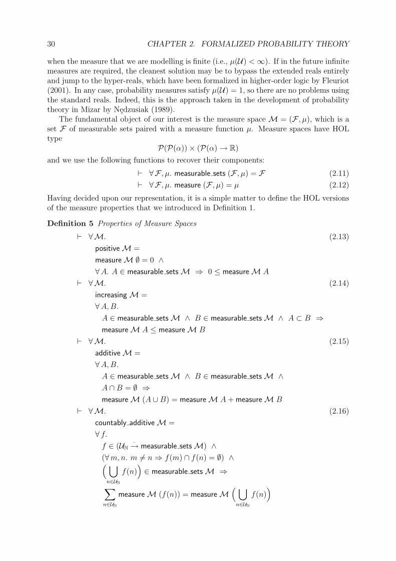
30 CHAPTER 2. FORMALIZED PROBABILITY THEORY
when the measure that we are modelling is finite (i.e., µ(U) <∞). If in the future infinitemeasures are required, the cleanest solution may be to bypass the extended reals entirelyand jump to the hyper-reals, which have been formalized in higher-order logic by Fleuriot(2001). In any case, probability measures satisfy µ(U) = 1, so there are no problems usingthe standard reals. Indeed, this is the approach taken in the development of probabilitytheory in Mizar by Nedzusiak (1989).
The fundamental object of our interest is the measure space M = (F , µ), which is aset F of measurable sets paired with a measure function µ. Measure spaces have HOLtype
P(P(α))× (P(α)→ R)
and we use the following functions to recover their components:
` ∀F , µ. measurable sets (F , µ) = F (2.11)
` ∀F , µ. measure (F , µ) = µ (2.12)
Having decided upon our representation, it is a simple matter to define the HOL versionsof the measure properties that we introduced in Definition 1.
Definition 5 Properties of Measure Spaces
` ∀M. (2.13)
positiveM =
measureM ∅ = 0 ∧∀A. A ∈ measurable setsM ⇒ 0 ≤ measureM A
` ∀M. (2.14)
increasingM =
∀A,B.A ∈ measurable setsM ∧ B ∈ measurable setsM ∧ A ⊂ B ⇒measureM A ≤ measureM B
` ∀M. (2.15)
additiveM =
∀A,B.A ∈ measurable setsM ∧ B ∈ measurable setsM ∧A ∩B = ∅ ⇒measureM (A ∪B) = measureM A+ measureM B
` ∀M. (2.16)
countably additiveM =
∀ f.f ∈ (UN
·→ measurable setsM) ∧(∀m,n. m 6= n⇒ f(m) ∩ f(n) = ∅) ∧( ⋃
n∈UN
f(n))∈ measurable setsM ⇒
∑n∈UN
measureM (f(n)) = measureM( ⋃
n∈UN
f(n))

2.2. MEASURE THEORY 31
Following Williams (1991), in the definition of countable additivity we assume thatthe countable union set is measurable.7
Some combinations of these properties imply others, and the most useful theorems ofthis kind are as follows:
` ∀M. (2.17)
algebra (measurable setsM) ∧ positiveM ∧ additiveM ⇒increasingM
` ∀M. (2.18)
algebra (measurable setsM) ∧ positiveM ∧countably additiveM ⇒additiveM
` ∀M, f. (2.19)
algebra (measurable setsM) ∧ positiveM ∧ increasingM ∧additiveM ∧ f ∈ (UN
·→ measurable setsM) ∧(∀m,n. m 6= n⇒ f(m) ∩ f(n) = ∅) ⇒summable (measureM f)
So assuming an algebra of measurable sets and a positive measure, we have that additivityimplies increasing, countable additivity implies additivity, and increasing and additiveimply that the sequence of disjoint set measures can be summed. This last result ishalfway toward showing that countable additivity holds, the only fact remaining to beshown is that the sum (which must now exist) is equal to the measure of the union ofthese disjoint sets.
We may now formalize the concept of a measure space.8
Definition 6 Measure Spaces
` ∀M. (2.20)
measure spaceM =
sigma algebra (measurable setsM) ∧ positiveM ∧countably additiveM
To speed up the development, some properties of measure spaces are also formalized,including a HOL version of the important Monotone Convergence Theorem.
7It is not necessary to assume the union set is measurable in the definition of additivity, since themeasurable sets always form an algebra whenever these properties are applied in our development.
8Using this property it would now be possible to define a new HOL type of α measure spaces (aninhabitant has measurable sets ∅ and U having measure 0 and 1 respectively—this is also a probabilityspace). This would have the positive effect of removing some side-conditions from theorems about measurespaces, but would require extra reasoning with the bijection functions for the new type. It was not clearthat a net gain in simplicity would result, and so we chose not to follow this route in the presentformalization.

32 CHAPTER 2. FORMALIZED PROBABILITY THEORY
Theorem 7 (Monotone Convergence Theorem)
` ∀M, A, f. (2.21)
measure spaceM ∧ f ∈ (UN·→ measurable setsM) ∧
(∀n. f(n) ⊂ f(suc n)) ∧ (A =⋃
n∈UN
f(n)) ⇒
limn→∞
(measureM (f(n))) = measureM A
The conditions on f in this theorem are stated as “(f(n))n monotonically convergesto A”, and often written as (f(n))n ↑ A.
2.2.2 Caratheodory’s Extension Theorem
Definition 6 tells us precisely what a measure space is, but offers little in the way ofhints on how to construct one. Since an algebra F is generally finitely representable, itis perhaps reasonable to believe that it will be possible to directly define a particularmeasure µ0 on sets in F , and prove that µ0 has the required properties of positivity andcountable additivity. However, if we cannot even write down the general form of a set inσ(F), then it is not at all clear how we can extend µ0 to a measure µ that is positive andcountably additive on σ(F). This is precisely what the celebrated extension theorem ofCaratheodory allows us to do.
Theorem 8 (Caratheodory’s Extension Theorem)
` ∀M0. (2.22)
algebra (measurable setsM0) ∧ positiveM0 ∧countably additiveM0 ⇒∃M.
(∀A.A ∈ measurable setsM0 ⇒ measureM A = measureM0 A) ∧
measurable setsM = sigma (measurable setsM0) ∧measure spaceM
Given an algebra A and a positive, countably additive measure µ0 on A, there exists ameasure space (σ(A), µ) such that µ = µ0 on A.
The proof of this theorem requires two new definitions. Firstly, given a set systemF and a measure function λ we may define the λ-system of F , which contains every setL ∈ F satisfying
∀A ∈ F . λ(L ∩ A) + λ(Lc ∩ A) = λ(A)
Secondly, we define an outer measure, which is positive, increasing and countably subad-ditive, where this last is the following property:
∀ (En). µ(⋃
n
En
)≤∑
n
µ(En)
2.2. MEASURE THEORY 33
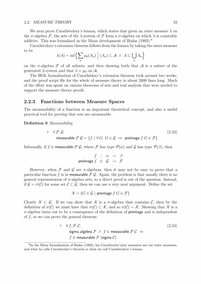
We next prove Caratheodory’s lemma, which states that given an outer measure λ onthe σ-algebra F , the sets of the λ-system of F form a σ-algebra on which λ is countablyadditive. This was formalized in the Mizar development of Bia las (1992).9
Caratheodory’s extension theorem follows from the lemma by taking the outer measureto be
λ(A) = inf∑
n
µ0(An)∣∣∣ (An) ⊂ A ∧ A ⊂
⋃n
An
on the σ-algebra F of all subsets, and then showing both that A is a subset of thegenerated λ-system and that λ = µ0 on A.
The HOL formalization of Carathedory’s extension theorem took around two weeks,and the proof script file for the whole of measure theory is about 2000 lines long. Muchof the effort was spent on various theorems of sets and real analysis that were needed tosupport the measure theory proofs.
2.2.3 Functions between Measure Spaces
The measurability of a function is an important theoretical concept, and also a usefulpractical tool for proving that sets are measurable.
Definition 9 Measurability
` ∀F ,G. (2.23)
measurable F G = f | ∀G. G ∈ G ⇒ preimage f G ∈ F
Informally, if f ∈ measurable F G, where F has type P(α) and G has type P(β), then
f : α → β
preimage f ∈ G ·→ F
However, when F and G are σ-algebras, then it may not be easy to prove that aparticular function f is in measurable F G. Again, the problem is that usually there is nogeneral representation of σ-algebra sets, so a direct proof is out of the question. Instead,if G = σ(C) for some set C ⊂ G, then we can use a very neat argument. Define the set
X = G ∈ G | preimage f G ∈ F
Clearly X ⊂ G. If we can show that X is a σ-algebra that contains C, then by thedefinition of σ(C) we must have that σ(C) ⊂ X , and so σ(C) = X . Showing that X is aσ-algebra turns out to be a consequence of the definition of preimage and is independentof f , so we can prove the general theorem:
` ∀ f,F , C. (2.24)
sigma algebra F ∧ f ∈ measurable F C ⇒f ∈ measurable F (sigma C)
9In the Mizar formalization of Bia las (1992), his Caratheodor’s[sic] measures are our outer measures,and what he calls Caratheodor’s theorem is what we call Caratheodory’s lemma.

34 CHAPTER 2. FORMALIZED PROBABILITY THEORY
In other words, instead of showing that the preimage of every set in the σ-algebra ismeasurable, we need only show this for a collection of sets that generate the σ-algebra.
We next define a useful extension of measurability, the property of a function beingmeasure-preserving.
Definition 10 Measure Preservation
` ∀M1,M2. (2.25)
measure preservingM1 M2 =
f |f ∈ measurable (measurable setsM1) (measurable setsM2) ∧∀A.A ∈ measurable setsM2 ⇒(measureM1 (preimage f A) = measureM2 A)
A function f is measure preservingM1 M2 if for each measurable set M2 of M2, thepreimage M1 under f of M2 satisfies:
• M1 is a measurable set of M1 (so f is measurable between the measurable sets ofM1 and M2);
• and the measure of M1 in M1 is the same as the measure of M2 in M2.
Analogously to the measurability property, we would like to show that
f ∈ measure preservingM (σ(C), µ)
reduces tof ∈ measure preservingM (C, µ)
by proving thatA ∈ σ(C) | measureM (preimage f A) = µ(A)
is a σ-algebra containing C.Unfortunately, whereas in the case of measurability this last step was an easy conse-
quence of the definition of preimage, for measure preservation it is not quite so straightfor-ward. The problem is showing closure under finite unions. Just because f preserves themeasure of A and B does not necessarily imply that f preserves the measure of A∪B. IfA and B are disjoint or one is a subset of the other then the result follows, but otherwiseit may not.
Thankfully, a standard result of measure theory comes to the rescue. A neat theoremgives an alternative characterization of σ(A) when A is an algebra.
Theorem 11 If A is an algebra, then σ(A) is the intersection of all sets F satisfying thefollowing conditions:
1. A ⊂ F
2. F is closed under complements.

2.2. MEASURE THEORY 35
3. F is closed under countable disjoint unions.
4. F is closed under countable increasing unions (where (En) is increasing if En ⊂ En+1
for every n).
Proof: Let G be the intersection of all F satisfying the above properties. First note thatG ⊂ σ(A), since σ(A) satisfies the properties. To show that σ(A) ⊂ G, we must showthat G is a σ-algebra containing A. Since one characterization of a σ-algebra is an algebraclosed under countable disjoint unions, the only difficulty is to show closure under unions.
Let X be the subset of G that is closed under unions with sets of the algebra A. Butthe algebra A is closed under unions, and so X satisfies the properties in the theorem,and so G ⊂ X . Therefore G = X , and so G is closed under unions with sets in the algebraA.
Now let Y be the subset of G that is closed under unions with all of the sets in G.As we have just proved, all of the sets in the algebra A are sets in Y , and so Y satisfiesthe properties of the theorem, thus G ⊂ Y . Therefore G = Y , and so G is closed underunions, as required. 2
It is easy to prove that the property of measure-preservation satisfies all of the condi-tions of Theorem 11, and so we can deduce the following theorem:
` ∀M1,M2,A, f. (2.26)
measure spaceM1 ∧ measure spaceM2 ∧ algebra A ∧(measurable setsM2 = sigma A) ∧f ∈ measure preservingM1 (A,measureM2) ⇒f ∈ measure preservingM1 M2
Therefore, instead of showing that f preserves the measure of every set in the σ-algebra,we need only show this for an algebra that generates the σ-algebra.
2.2.4 Probability Spaces
A probability space is a measure space where the measure of the whole space is 1. Ina probability space, the measurable sets are called events, and the measure is called aprobability.
Definition 12 Probability Spaces
` ∀M. (2.27)
prob spaceM = measure spaceM ∧ measureM U = 1
` events = measurable sets (2.28)
` prob = measure (2.29)
` prob preserving = measure preserving (2.30)
These definitions of events, prob and prob preserving indicate our technique for dealingwith the change in terminology between measure theory and probability theory. Ratherthan conventionally re-using the existing constants, which would lead to a rather confusing
36 CHAPTER 2. FORMALIZED PROBABILITY THEORY
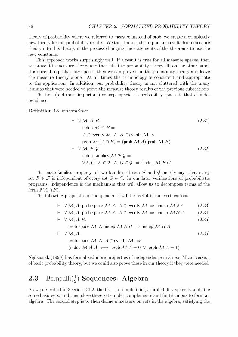
theory of probability where we referred to measure instead of prob, we create a completelynew theory for our probability results. We then import the important results from measuretheory into this theory, in the process changing the statements of the theorems to use thenew constants.
This approach works surprisingly well. If a result is true for all measure spaces, thenwe prove it in measure theory and then lift it to probability theory. If, on the other hand,it is special to probability spaces, then we can prove it in the probability theory and leavethe measure theory alone. At all times the terminology is consistent and appropriateto the application. In addition, our probability theory in not cluttered with the manylemmas that were needed to prove the measure theory results of the previous subsections.
The first (and most important) concept special to probability spaces is that of inde-pendence.
Definition 13 Independence
` ∀M, A,B. (2.31)
indepM A B =
A ∈ eventsM ∧ B ∈ eventsM ∧probM (A ∩B) = (probM A)(probM B)
` ∀M,F ,G. (2.32)
indep familiesMF G =
∀F,G. F ∈ F ∧ G ∈ G ⇒ indepM F G
The indep families property of two families of sets F and G merely says that everyset F ∈ F is independent of every set G ∈ G. In our later verifications of probabilisticprograms, independence is the mechanism that will allow us to decompose terms of theform P(A ∩B).
The following properties of independence will be useful in our verifications:
` ∀M, A. prob spaceM ∧ A ∈ eventsM ⇒ indepM ∅ A (2.33)
` ∀M, A. prob spaceM ∧ A ∈ eventsM ⇒ indepM U A (2.34)
` ∀M, A,B. (2.35)
prob spaceM ∧ indepM A B ⇒ indepM B A
` ∀M, A. (2.36)
prob spaceM ∧ A ∈ eventsM ⇒(indepM A A ⇐⇒ probM A = 0 ∨ probM A = 1)
Nedzusiak (1990) has formalized more properties of independence in a neat Mizar versionof basic probability theory, but we could also prove these in our theory if they were needed.
2.3 Bernoulli(12) Sequences: Algebra
As we described in Section 2.1.2, the first step in defining a probability space is to definesome basic sets, and then close these sets under complements and finite unions to form analgebra. The second step is to then define a measure on sets in the algebra, satisfying the
2.3. BERNOULLI(12) SEQUENCES: ALGEBRA 37
conditions of positivity and countable additivity. At this point, we are in a position toapply Caratheodory’s extension theorem to this measure and yield the final probabilityspace. In this section we develop the necessary theory to define an algebra of sets ofsequences, and a measure function on these sets that respects our intuition that “everysequence is equally likely to occur”.
However, the relationship of this theory to the eventual theory of probability is notmerely a bootstrapping one, as for example the theory of positive reals is to the theoryof reals. Rather, we intend to use the theorems of Section 2.2.3 to solve problems ofmeasurability and measure-preservation of probabilistic programs. This will involve re-ducing problems on the σ-algebra to equivalent problems on the algebra,10 and so we mustensure that our algebra theory is equipped with the useful lemmas needed for practicalverification.
Although the previous section was a direct formalization of measure theory from thetextbook of Williams (1991), at this point our formalization diverges from his treatment.In the theorem-prover we must be more concerned with the representation of sets ofinfinite bit sequences, so that later we can use this theory to directly prove propertiesof probabilistic programs. This work therefore represents a novel way to develop theprobability space of an infinite sequence of coin-flips: in textbooks this is normally madefully rigorous by defining the space as an infinite product of a single coin-flip.11
2.3.1 Infinite Sequence Theory
As usual in higher-order logic modelling, the initial decisions are concerned with choosingtypes to model our objects. In this case we represent infinite bit sequences with functionsN → B. The intuition is that if s models a bit sequence, then s(n) = > means that thenth bit in the sequence is 1, and s(n) = ⊥ means that the nth bit is 0.
Generalizing slightly, we develop a theory of infinite α-sequences modelled by the typeN → α, where α is any higher-order logic type. Our guide here is the theory of lists,and we define sequence analogues of the list functions hd, tl, cons, take and drop.12 Wealso define sdest which gives the head and tail of the sequence as a pair; this will be asurprisingly useful probabilistic program!
Definition 14 Basic Sequence Operations
` ∀ s. shd s = s 0 (2.37)
` ∀ s. stl s = s suc (2.38)
` ∀ a, s, n. scons a s 0 = a ∧ scons a s (suc n) = s n (2.39)
` ∀n, s. (2.40)
stake 0 s = [ ] ∧ stake (suc n) s = cons (shd s) (stake n (stl s))
` ∀n, s. sdrop 0 s = s ∧ sdrop (suc n) s = sdrop n (stl s) (2.41)
` ∀ s. sdest s = (shd s, stl s) (2.42)
10This is how the measurability theorems in Section 2.4.2 were proved.11We could also have used infinite products to define the probability space, but this path would have
required formalizing many more theorems of measure theory.12Of course, there is no analogue of [ ] or length, since these are infinite sequences.

38 CHAPTER 2. FORMALIZED PROBABILITY THEORY
Another useful generic construct is the following definition, which creates a sequencefrom an observation and an iteration function.
Definition 15 Constructing a Sequence from an Iteration Function
` ∀h, t, x. siter h t x = scons (h(x)) (siter h t (t(x))) (2.43)
So for example, siter I suc 0 is the sequence (0, 1, 2, 3, . . .).
We also define a mirror sequence operation specific to boolean sequences: this mapsthe sequence (x0, x1, x2, . . .) to (¬x0, x1, x2, . . .).
Definition 16 The mirror Sequence Operation
` ∀ s. mirror s = scons (¬(shd s)) (stl s) (2.44)
Finally, we prove some basic properties of sequences, to expedite proofs and to avoidusing their underlying representation as functions.
` ∀h, t. shd (scons h t) = h (2.45)
` ∀h, t. stl (scons h t) = t (2.46)
` ∀ s. ∃h, t. s = scons h t (2.47)
` ∀ s. scons (shd s) (stl s) = s (2.48)
` ∀h, h′, t, t′. scons h t = scons h′ t′ ⇐⇒ h = h′ ∧ t = t′ (2.49)
` ∀ s. mirror (mirror s) = s (2.50)
` ∀ s. stl (mirror s) = stl s (2.51)
In the succeeding theory, all of the infinite sequences we meet will be infinite booleansequences.
2.3.2 The Algebra Generated by Prefix Sets
We set the prefix sets to be the generating sets of an algebra A.
Definition 17 Prefix Sets
` ∀ l. prefix set l = s | stake (length l) s = l (2.52)
` ∀h, t. prefix seq (cons h t) = scons h (prefix seq t) (2.53)
So prefix set l is the set of all sequences that have initial segment l, and prefix seq l is thecanonical sequence of prefix set l.13
Since the prefix sets do not naturally form an algebra (for example, the empty setcannot be represented as a prefix set), it is necessary to close the prefix sets under com-plements and finite unions. For this we shall use an embedding function from boolean listlists to sets of sequences.
13Note the use of a pattern match definition to fix only the cons case, allowing the [ ] case to assumean arbitrary value.
2.3. BERNOULLI(12) SEQUENCES: ALGEBRA 39
Definition 18 An Embedding Function
` ∀ l. embed [l0, . . . , ln−1] =⋃
0≤i<n
prefix set li (2.54)
We may now define what it means to be a set in A.
Definition 19 The Bernoulli(12) Algebra
` A = A | ∃ l. embed l = A (2.55)
At the moment we do not have all the machinery we will use to prove that A isan algebra. Showing closure under complements is not trivial, and it will be the firstapplication of our induction principle on canonical forms, described in Section 2.3.3.
The second step in our probability space construction is to define a measure on thesets in A. We begin with the intuition that all sequences are equally likely, so given twolists l, l′ of the same length we would expect the measure of prefix set l to be the same asthe measure of prefix set l′. Pursuing the consequences of this, there are 2n boolean listsof length n, and each sequence falls into exactly one of the prefix sets resulting from theselists, so we therefore define the measure of prefix set l to be 2−(length l).
We can extend this to a measure µ on a general set in A.
Definition 20 A Measure on Sets in A
` ∀ l. µ0[l0, . . . , ln−1] =∑
0≤i<n
2−(length li) (2.56)
` ∀A. µ(A) = infµ0(l) | embed l = A (2.57)
We have to be rather careful in this definition, because for a given A ∈ A there maybe many l : B∗∗ with embed l = A. As an example, both [[>]] and [[>,>], [>,⊥], [>,>]]embed to the set of all sequences beginning with >. The definition works around this bypicking the infimum, and since for every l : B∗∗ we have that 0 ≤ µ0(l) this infimum isalways well-defined for sets in A.14
2.3.3 Canonical Forms
In the previous subsection we set out all the definitions for the algebra A of booleansequence sets, and the measure µ from sets in the algebra to real numbers. Followingour program for applying measure theory, the next step is to prove that A is an algebraand that (A, µ) is positive and countably additive. We will then be ready to apply theextension theorem.
Unfortunately, the definitions of A and µ do not directly lend themselves to routineproofs in the HOL theorem prover, most of which are performed using an induction schemeof one kind or another.15 In particular, the definition of µ as the infimum of a set of real
14This follows immediately from the fact that we are working in the real numbers, though it will laterturn out that for every A ∈ A there is always an l : B∗∗ with embed l = A and µ0(l) = µ(A).
15One sizeable exception to this generalization is the theory of real analysis, where there is also noinduction scheme available.

40 CHAPTER 2. FORMALIZED PROBABILITY THEORY
numbers is particularly difficult to work with, since at least at first sight we have no ideawhich boolean list lists that embed to a particular set in the algebra are resulting in thesmall measures. We cannot even easily calculate µ(U), the measure of the whole algebra.Even though embed [[ ]] = U and µ0([[ ]]) = 20 = 1, there may also be another l : B∗∗ withembed l = U and µ0(l) < 1.
To resolve this, we introduce a (computable) canonicalization function canon : B∗∗ →B∗∗.
Definition 21 Canonical Forms
` ∀ l. (2.58)
(∀ l′. embed l′ = embed l ⇐⇒ canon l′ = canon l) ∧µ0(canon l) ≤ µ0(l)
` ∀ l. canonical l ⇐⇒ canon l = l (2.59)
In other words, the canonical form canon l is a representative of all boolean list lists thatembed to embed l, and the representative chosen has minimal measure.
This gives us a more tractable characterization of the measure µ:
` ∀ l. µ(embed l) = µ0(canon l) (2.60)
So to find the probability of a set A ∈ A, it suffices to find any l : B∗∗ with embed l = A,evaluate canon l in the logic, and then deduce that µ(A) = µ0(canon l).
It is not necessary to describe in detail the HOL definition of canon and the subsequentderivation of the characterizing property (2.58), but it may provide some insight to explainthe three steps of the canonicalization function canon:
1. The input list l is sorted according to an order defined on B∗.
2. If there is an element x of l that is a prefix of another element y of l, then y is removedfrom l. This is a valid step (i.e., it preserves embed l) because embed y ⊂ embed x(as can be seen from Definition 17).
3. Elements are merged with their twins, where the lists x and y are twins with parentz if x = append z [>] and y = append z [⊥]. If elements x and y of l are twins withparent z, then x is removed and y is replaced by z. This is also a valid step, sinceembed z = embed x ∪ embed y.
The only difficulty is choosing the order function in step 1 so that the list is kept in orderafter an application of step 3.16
The canonicalization algorithm is useful not only for evaluating measures, it also givesus an induction principle on elements of the algebra A. Since elements of A correspondto the underlying list type B∗∗, the standard list induction principle17 is also applicable,but this does not fit well with the natural structure of our sequence space B∞, where wewould like to use the sequence operators shd and stl to reduce a goal to the inductionhypothesis. Here is the induction principle for lists in canonical form:
16Note that using sets instead of lists does not obviate the need for canonicalization, because elementswould still need to be merged with their twins.
17Captured by the theorem: ` ∀Q. Q([ ]) ∧ (∀h, t. Q(t)⇒ Q(cons h t)) ⇒ ∀ l. Q(l).

2.3. BERNOULLI(12) SEQUENCES: ALGEBRA 41
Theorem 22 Canonical Form Induction Principle
` ∀Q. (2.61)
Q([ ]) ∧ Q([[ ]]) ∧(∀ l, l′.
canonical l ∧ canonical l′ ∧ Q(l) ∧ Q(l′) ∧canonical (append (map (cons >) l) (map (cons ⊥) l′)) ⇒Q(append (map (cons >) l) (map (cons ⊥) l′))) ⇒∀ l. canonical l ⇒ Q(l)
The base cases are the lists [ ] (embedding to the empty set) and [[ ]] (embedding tothe whole space U); the step case builds a list in canonical form from two others l, l′. Formany goals we can prove the step case with a case split on the head of some sequence,followed by some rewriting with l or l′ as appropriate.
2.3.4 Properties of (A, µ)
The first application of the canonical form induction principle is to show that A is analgebra, satisfying the HOL definition of an algebra we made in Definition 4. The proofof this in HOL is instructive in its use of the induction principle, and so we give a sketch.
Theorem 23 A is an Algebra
` algebra A (2.62)
Proof: It is clear that ∅ ∈ A (from the embedding of [ ]), and given two sets A,B ∈ Awhich were embedded from the lists lA, lB, it is easy to see that the list append lA lB embedsto the union A ∪ B. The only difficulty is to show that A is closed under complements.Suppose we have A ∈ A which embeds from the list lA. Since A is also the embeddingof canon lA, we can assume that lA is in canonical form. If it is either [ ] or [[ ]] then theother embeds to Ac, so we may assume that there exist l, l′ with
lA = append (map (cons >) l) (map (cons ⊥) l′)
By the induction hypothesis the embedding of l has a complement in A, say it wasembedded from the list lc. Similarly there exists l′c for l′. It is now not difficult to showthat
append (map (cons >) lc) (map (cons ⊥) l′c)
embeds to Ac, as required. 2
Using similar arguments, we prove that (A, µ) is positive, additive, and even countablyadditive. This last follows from a neat property of the algebra A:
` ∀ f. (2.63)
f ∈ (UN·→ A) ∧ (∀m,n. m 6= n⇒ f(m) ∩ f(n) = ∅) ∧( ⋃
n∈UN
f(n))∈ A ⇒
∃N. ∀n. N ≤ n⇒ f(n) = ∅

42 CHAPTER 2. FORMALIZED PROBABILITY THEORY
Any countable sequence of disjoint sets in A that union to a set in A contains only a finitenumber of non-empty sets. Thus in the case of (A, µ), countable additivity collapses toadditivity.
An interesting property we prove is that the measure µ has an upper bound of 1:
` ∀A. A ∈ A ⇒ µ(A) ≤ 1 (2.64)
This is a special case of Kraft’s Inequality (Goldie and Pinch, 1991):
∀C.∑w∈C
a−(length w) ≤ 1 (2.65)
which holds for all prefix-free codes C where the alphabet has a symbols, and exactlyformulates the balance between keeping the code prefix-free and having many short codewords. In our situation we have ‘code words’ of boolean lists (so a = 2), and for thepurpose of calculating µ we can assume that our ‘code’ is in canonical form (and henceprefix-free).
2.4 Bernoulli(12) Sequences: Probability Space
2.4.1 The Need for σ-algebras
In the previous section we defined an algebra A with associated measure µ, establishedan induction principle to expedite proofs in the algebra, and proved that (A, µ) satisfiesthe basic properties of measures.
For a probabilistic program f : B∞ → α × B∞ that is guaranteed to terminate, all ofthe interesting behaviour of f can be captured using sets of A.18 In a previous versionof our probability theory (Hurd, 2000), we were able to verify some simple probabilisticprograms using only (A, µ).
However, probabilistic programs that are guaranteed to terminate are a relatively smallclass, and there are many interesting programs that cannot be expressed with this restric-tion. An example is the program f that scans the input sequence for the first occurrenceof a ⊥, and returns the index (counting from 0) of this ⊥ within the sequence.19 Althoughthe probability that f terminates is 1, termination is nevertheless not guaranteed: thesequence (>,>, . . .) results in divergence.20 Now consider the set S of input sequencesthat result in f returning an even number:
S = prefix set [⊥] ∪ prefix set [>,>,⊥] ∪ prefix set [>,>,>,>,⊥] ∪ · · ·
Although S is a countable union of sets in A, it is not itself a set in A. Therefore, sinceµ is only defined on sets in A, we cannot speak of the probability µ(S) that f returns aneven number. On the other hand, σ-algebras are closed under countable unions, so if we
18If f is guaranteed to terminate then there is a number n such that whatever sequence s is input tof , no more than the initial n bits of s will be used by f to calculate a result.
19This is the Geometric(12 ) distribution, and we study this in detail in Section 4.4.
20Using the argument of Footnote 18, the fact that the set of possible results forms an infinite set alsoproves that f cannot be guaranteed to terminate.

2.4. BERNOULLI(12) SEQUENCES: PROBABILITY SPACE 43
extend the measure µ to be defined on σ(A), then S is an event and the probability of Sbecomes meaningful.
The conclusion is that A allows us to reason about probabilistic programs that areguaranteed to terminate, but σ(A) is required to reason about programs that terminatewith probability 1.
2.4.2 Definition of the Probability Space
The properties of (A, µ) established in Section 2.3.4 are precisely the conditions requiredby Caratheodory’s extension theorem, which we formalized in Section 2.2.2. Applying thetheorem, we can define the probability space (E ,P) and prove the following characterizingtheorem.
Definition 24 The Probability Space of Bernoulli(12) Sequences
` prob space (E ,P) ∧ (E = sigma A) ∧ (2.66)
∀A. A ∈ A ⇒ P(A) = µ(A)
Now using the properties of probability spaces, some standard theorems follow, in-cluding the result that any countable set of sequences has probability 0:
` ∀A. countable A ⇒ A ∈ E ∧ P(A) = 0 (2.67)
Therefore, for any event E ∈ E , adding or taking away a countable set of sequences doesnot change the probability of E. In particular, if we start with the whole space U , and forevery list l : B∗ we remove the sequence with initial segment l and continuing (>,>, . . .),then the set Θ we are left with still has probability 1.21
This result justifies the intuition we gain by the identification of bit sequences withreal numbers via the binary expansion
(x0, x1, x2, . . .)φ−→ 0. x0 x1 x2 · · ·
even though there are some distinct sequences (such as (0, 1, 1, 1, . . .) and (1, 0, 0, 0, . . .))that map to the same real number.22 The set Θ, an event of probability 1, is in one-to-one correspondence with the real numbers in the interval [0, 1).23 Though we do notpursue the consequences of this here, it is possible to define Lebesgue integration for a setS ⊂ [0, 1] of reals by
Leb(S) = P(preimage φ S)
We now prove some important properties of the sequence operations, showing howthey map events and change their probabilities. The proof technique is always the same:
21This result is the intuitively correct one. In our previous version of probability theory (Hurd, 2000)where we were limited to (A, µ), we defined the probability of a set B to be the supremum of all µ(A)where A ∈ A and A ⊂ B. Unfortunately, the only set in A that is a subset of Θ is the empty set, and sothe probability of Θ was set to 0.
22This same complication rears its ugly head in the proof of Cantor’s theorem that the real numbersare uncountable, which is why proofs normally use decimal expansions!
23This is from (Williams, 1991, page 42): every real number in (0, 1) has one bit sequence mapping toit, except for the dyadic rationals which have two. The sequences missing from the set Θ are easily seento be in one-to-one correspondence with the dyadic rationals.
44 CHAPTER 2. FORMALIZED PROBABILITY THEORY
use the theorems of Section 2.2.3 to reduce a property over E to a property over A, andfrom there use the canonical form induction principle of Section 2.3.3.
Firstly, we tackle measurability and stronger properties of eventhood:
` ∀ b. s | shd s = b ∈ E (2.68)
` ∀E. preimage stl E ∈ E ⇐⇒ E ∈ E (2.69)
` ∀E. E ∈ E ⇒ image stl E ∈ E (2.70)
` ∀E, n. preimage (sdrop n) E ∈ E ⇐⇒ E ∈ E (2.71)
` ∀E, n. E ∈ E ⇒ image (sdrop n) E ∈ E (2.72)
` ∀ b. scons b ∈ measurable E E (2.73)
` ∀E, b. image (scons b) E ∈ E ⇐⇒ E ∈ E (2.74)
` ∀E. preimage mirror E ∈ E ⇐⇒ E ∈ E (2.75)
These theorems are all as strong as possible, counter-intuitive though this may appear.For example, the plausible-looking statement
image stl E ∈ E ⇒ E ∈ E
fails because of the counterexample
E = image (scons >) U ∪ image (scons ⊥) Ω
where Ω is any non-measurable set (we shall explicitly construct a non-measurable set inSection 2.4.3). The image of E under stl is U ∈ E , but if E were measurable then usingtheorems (2.68) and (2.74) it would be possible to show that Ω was measurable.
Note that we do not need a theorem about images of mirror, because
` image mirror = preimage mirror (2.76)
We also prove some probability preservation properties:
` ∀ b. P s | shd s = b = 12
(2.77)
` stl ∈ prob preserving E E (2.78)
` ∀n. sdrop n ∈ prob preserving E E (2.79)
` mirror ∈ prob preserving E E (2.80)
` ∀E. (2.81)
E ∈ E ∧ image mirror E = E ⇒ P(image stl E) = P(E)
Finally, once we have the basic properties of the sequence operations, we can provethe following two theorems:
` ∀n. P s | shd (sdrop n s) = 12
(2.82)
` ∀m,n. (2.83)
P s | shd (sdrop m s) = shd (sdrop n s) = if m = n then 1 else 12
These say that the probability of any random bit being 1 is 12
(2.82), and the probabilityof two distinct random bits being equal is also 1
2(2.83). Since these are the results we
would expect for a sequence of coin flips, this gives us confidence that the probabilityspace (E ,P) we have defined in this section is a good model for a random bit generator.
2.4. BERNOULLI(12) SEQUENCES: PROBABILITY SPACE 45
2.4.3 Construction of a Non-Measurable Set
The purpose of this section is to define a set Ω of sequences, and prove the theorem
` Ω /∈ E (2.84)
that Ω is not an event of our probability space.This represents a digression from the focus of this chapter, which is to formalize theory
that will support verifications of probabilistic programs. It is, however, a theoreticallyimportant result, justifying the route through measure theory that our theory has taken,and providing a tool for generating counter-examples. Ironically, since σ-algebras areso successful at capturing the events of interest to probability theory, it is not easy toconstruct a set that is provably not an event.
We adapt a construction in Williams (1991, page 192) of a non-measurable set A ⊂ S1,where S1 is the unit circle. The argument begins as follows:
. . . we use the Axiom of Choice to show that
S1 =⋃q∈Q
Aq
where the Aq are disjoint sets, each of which may be obtained from any of the othersby rotation. If the set A = A0 has a ‘length’, then it is intuitively clear that [theabove result] would force
2π =∞× length(A),
an impossibility.
The important parts of this are:
1. The Axiom of Choice is used to construct the non-measurable set A.
2. There is a mapping that deterministically changes the measure of sets (in this caserotations preserve length).
3. The whole space is written as a disjoint union of countably many rotations of A.
We now transfer these ideas to sets of boolean sequences. For step 1 of the aboveoutline we use the eventually relation between sequences.
Definition 25 The ‘Eventually’ Sequence Relation
` ∀x, y. eventually x y = ∃n. sdrop n x = sdrop n y (2.85)
The sequence x is eventually the sequence y if they disagree only on some initial segment;eventually can be shown to be an equivalence relation.
Definition 26 A Non-Measurable Set
` ∀x. ∃! y. eventually x y ∧ y ∈ Ω (2.86)

46 CHAPTER 2. FORMALIZED PROBABILITY THEORY
The set Ω consists of equivalence class representatives of the eventually relation.24
For step 2, we consider the sequence of sets
Ωn = preimage (sdrop n) (image (sdrop n) Ω)
Assuming Ω is an event, and using theorems (2.79) and (2.81), it can be shown that
P(Ωn) = 2nP(Ω)
Since probabilities are always bounded above by 1, we must have that
P(Ω) = 0
For step 3, we first prove a lemma that the sequence Ωn monotonically converges tothe whole space U , or
Ωn ⊂ Ωn+1 ∧ U =⋃
n∈UN
Ωn
Now the Monotone Convergence Theorem may be applied, allowing
0 = limn→∞
0 = limn→∞
2nP(Ω) = limn→∞
P(Ωn) = P(U) = 1
and we may conclude that Ω is not an event of the probability space.
2.4.4 Probabilistic Quantifiers
In probability textbooks, it is common to find many theorems with the qualifier ‘almostsurely’, ‘with probability 1’ or just ‘w.p. 1’. Intuitively, this means that the set of pointsfor which the theorem is true has probability 1 (the set and the probability space usuallybeing implied by context). We can define probabilistic versions of the ∀ and ∃ quantifiersthat make this notation precise.25
Definition 27 Probabilistic Quantifiers
` ∀φ. (∀∗s. φ(s)) = s | φ(s) ∈ E ∧ P s | φ(s) = 1 (2.88)
` ∀φ. (∃∗s. φ(s)) = s | φ(s) ∈ E ∧ P s | φ(s) 6= 0 (2.89)
As noted by Harrison (1996a) on the subject of variable binding in mathematics,“[formalization] really can be valuable, confronting us with awkward constructs where theeveryday notation confuses free and bound variables or a function with its value.” Herewe have an opportunity of making precise a (potentially) confusing everyday notation, butthe familiar use of quantifiers for binding avoids the necessity of an awkward construct.
24Theorem (2.86) is a characterizing theorem; the actual definition of Ω explicitly invokes the Axiomof Choice (in the form of Hilbert’s choice operator ε):
` Ω = image (λ x. ε y. eventually x y) U (2.87)
25We pronounce ∀∗ as “probably” and ∃∗ as “possibly”.
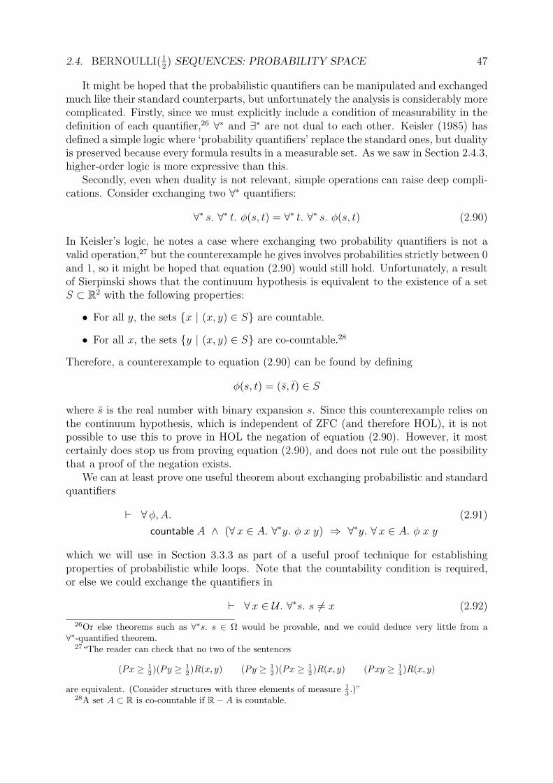
2.4. BERNOULLI(12) SEQUENCES: PROBABILITY SPACE 47
It might be hoped that the probabilistic quantifiers can be manipulated and exchangedmuch like their standard counterparts, but unfortunately the analysis is considerably morecomplicated. Firstly, since we must explicitly include a condition of measurability in thedefinition of each quantifier,26 ∀∗ and ∃∗ are not dual to each other. Keisler (1985) hasdefined a simple logic where ‘probability quantifiers’ replace the standard ones, but dualityis preserved because every formula results in a measurable set. As we saw in Section 2.4.3,higher-order logic is more expressive than this.
Secondly, even when duality is not relevant, simple operations can raise deep compli-cations. Consider exchanging two ∀∗ quantifiers:
∀∗ s. ∀∗ t. φ(s, t) = ∀∗ t. ∀∗ s. φ(s, t) (2.90)
In Keisler’s logic, he notes a case where exchanging two probability quantifiers is not avalid operation,27 but the counterexample he gives involves probabilities strictly between 0and 1, so it might be hoped that equation (2.90) would still hold. Unfortunately, a resultof Sierpinski shows that the continuum hypothesis is equivalent to the existence of a setS ⊂ R2 with the following properties:
• For all y, the sets x | (x, y) ∈ S are countable.
• For all x, the sets y | (x, y) ∈ S are co-countable.28
Therefore, a counterexample to equation (2.90) can be found by defining
φ(s, t) = (s, t) ∈ S
where s is the real number with binary expansion s. Since this counterexample relies onthe continuum hypothesis, which is independent of ZFC (and therefore HOL), it is notpossible to use this to prove in HOL the negation of equation (2.90). However, it mostcertainly does stop us from proving equation (2.90), and does not rule out the possibilitythat a proof of the negation exists.
We can at least prove one useful theorem about exchanging probabilistic and standardquantifiers
` ∀φ,A. (2.91)
countable A ∧ (∀x ∈ A. ∀∗y. φ x y) ⇒ ∀∗y. ∀x ∈ A. φ x y
which we will use in Section 3.3.3 as part of a useful proof technique for establishingproperties of probabilistic while loops. Note that the countability condition is required,or else we could exchange the quantifiers in
` ∀x ∈ U . ∀∗s. s 6= x (2.92)
26Or else theorems such as ∀∗s. s ∈ Ω would be provable, and we could deduce very little from a∀∗-quantified theorem.
27“The reader can check that no two of the sentences
(Px ≥ 12 )(Py ≥ 1
2 )R(x, y) (Py ≥ 12 )(Px ≥ 1
2 )R(x, y) (Pxy ≥ 14 )R(x, y)
are equivalent. (Consider structures with three elements of measure 13 .)”
28A set A ⊂ R is co-countable if R−A is countable.

48 CHAPTER 2. FORMALIZED PROBABILITY THEORY
to get∀∗s. ∀x. s 6= x
which is equivalent to
(∀∗s. ⊥) ⇐⇒ ∅ ∈ E ∧ (P(∅) = 1) ⇐⇒ >∧ (0 = 1) ⇐⇒ ⊥
So far we have presented these probabilistic quantifiers as a notational device, a preciseand still intuitive version of the tag ‘with probability 1’. However, we have discovered onesituation where the use of ∀∗ represents more than just a useful shorthand: it also speedsup the proof. The technique uses a lifting theorem for ∀∗-quantified properties.
Theorem 28 The ∀∗-lifting Theorem.
` ∀φ,E,E ′. (2.93)
E ∈ E ∧ E ′ ∈ E ∧ ∀∗φ ∧ (∀x. φ(x)⇒ (x ∈ E ⇐⇒ x ∈ E ′)) ⇒P(E) = P(E ′)
This says that that the probability of the set E is equal to the probability of E ′ ifwe can transform E to E ′ by regarding as universally true any probabilistic universallyquantified property φ. In this way a ∀∗-theorem gets lifted to a ∀-theorem in the argumentof a P.29
Example: Suppose we wish to prove
P s | shd s ∧ s 6= y = P s | shd s
By specializing the ∀∗-lifting theorem to the ∀∗-quantified property in theorem (2.92)above, it remains only to prove that
s | shd s ∧ s 6= y ∈ E ∧ s | shd s ∈ E ∧∀x. x 6= y ⇒ (x ∈ s | shd s ∧ s 6= y ⇐⇒ x ∈ s | shd s)
which is easily accomplished using the measurability properties of shd. 2
Before we proved the ∀∗-lifting theorem, we would have to prove these kind of resultsby explicitly constructing an event S of probability 1, and then use set operations to show
P(E) = P(E ∩ S) = P(E ′ ∩ S) = P(E ′)
In our experience, this ‘bare-hands’ approach generally results in more work.
2.5 Concluding Remarks
The main result of this chapter is the measure-theoretic construction of the probabilityspace (E ,P). Chapter 3 will use the properties of (E ,P) we have formalized to specify andverify some probabilistic algorithms.
29Another way of seeing the ∀∗-lifting theorem is as a congruence rule for P, though it can’t be givento a HOL simplifier in its current form with φ left unspecified.
2.5. CONCLUDING REMARKS 49
There have been several semantics of probabilistic programs presented in the literatureof theoretical computer science. Most of them use measure theory in a more or lessdirect way, to avoid falling into the logical inconsistencies of the Banach-Tarski paradox.Therefore, to formalize one of these semantics in a theorem prover, measure theory (ora particular specialization) must be formalized also. This is the novelty of this chapter:measure theory as a definitional extension of higher-order logic, intended to support ourown simple semantics of probabilistic programs.
Much of the technical work in this chapter was anticipated in the Mizar develop-ments of Nedzusiak (1989) and Bia las (1990), but there are many situations (such asCaratheodory’s extension theorem) in which we have had to go a little further into thetheory to extract the particular theorems that our application requires. The formal con-struction of a non-measurable set is a novelty, as is the introduction of probabilisticquantifiers into a standard logic.
Our formalized probability theory allows us to express both standard logical truths andprobabilistic statements in higher-order logic. There has been some theoretical work onthe various techniques of combining various (first-order) logics and probability to achievethis effect: papers of Halpern (1990) and Abadi and Halpern (1994) give some decidabilityand complexity results. Another approach is taken in the fuzzy logic of Zadeh (1965),where the truth values are extended from the booleans ⊥,> ∼= 0, 1 to the wholereal interval [0, 1]. The logical connectives are also extended to operate over the largerdomain: although this extension is necessarily rather arbitrary, there are neverthelessmany control systems that internally make use of fuzzy logic to operate robustly in achanging environment. There is also a probabilistic logic due to Nilsson (1986), which isa version of fuzzy logic where the truth values correspond to probabilities. In this casethe logical connectives are not simple functions of real numbers, instead the entailmentrelation must be calculated by multiplying matrices together.
We used the hol98 theorem prover to do this work, creating a purely definitionaltheory to ensure soundness (in common with most other hol98 theories). Particularlyimportant for this work were the theories of real numbers (created by Harrison (1998))and predicate sets, although of course we found invaluable the basic theories of arithmetic,lists, well-founded recursion and the like. The built-in proof tools of hol98 sped up thewhole development, which makes heavy use of the simplifier, first-order prover and realnumber decision procedure. However, although these tools make a big difference to thetask of ‘proving the current subgoal’, we should not forget the higher-level issues that alsosped up this development:
• Picking the right higher-order logic types to represent our objects. It would perhapshave been more natural to model bit sequences with number sequences instead of theboolean sequences we chose, but this would have resulted in extra well-formednessconditions guaranteeing that only the numbers ‘1’ and ‘0’ were present.
• Higher-order theorems capturing common patterns of reasoning should be activelysought. We ‘discovered’ the Canonical Form Induction Principle quite late in thedevelopment, and when we cleaned up the proofs of the earlier theorems usingthe new technique, the proof scripts shrunk dramatically and many lemmas wererendered obsolete.

50 CHAPTER 2. FORMALIZED PROBABILITY THEORY

Chapter 3
Verifying Probabilistic Algorithms
We present a simple model of probabilistic algorithms in higher-order logic, in which it ispossible to express any program with access to a source of random bits. The formalizationof probability theory allows us to make meaningful specifications of these algorithms, andwe develop the formal framework to make verification in the theorem prover more straight-forward. One novelty is a compositional property of probabilistic algorithms that impliesmeasurability and independence. Finally, we examine various schemes of probabilistictermination with reference to our own probabilistic while loop.
3.1 Introduction
3.1.1 Motivating Probabilistic Algorithms
The study of probabilistic algorithms grew out of the Monte Carlo simulation methodsused in numerical analysis and statistical physics.1 The first formal model of probabilisticcomputation was proposed in a paper of de Leeuw et al. (1955), followed by the pioneeringwork of Rabin (1963), Karp (1976) and Gill (1977). Today probabilistic algorithms arewell-established in computer science, and there are many examples of simple probabilis-tic algorithms that outperform all known deterministic alternatives. To illustrate thisphenomenon, which best conveys the advantages of probabilistic algorithms, consider thefollowing two problems:
1. Given two sets of polynomials over Q
P1, . . . , Pm and Q1, . . . , Qn
where each polynomial is represented by a list of the non-zero terms, we wish toknow if ∏
1≤i≤m
Pi 6=∏
1≤i≤n
Qi
1An early example of Monte Carlo methods used in the sciences is the classic experiment of Buffon(1777) where the value of π is approximated by repeatedly dropping a needle onto a surface marked withparallel lines. If the lines are exactly one needle’s length apart, then the probability that the needle willintersect a line is 2/π.
51

52 CHAPTER 3. VERIFYING PROBABILISTIC ALGORITHMS
2. How can the pivot be picked in quicksort so that the sorting algorithm has a fastexpected running time?
Problem 1 is known in the complexity literature as Product Polynomial Inequiv-alence. It has no known polynomial time solution,2 but it can be solved in expectedpolynomial time:
• pick an x in some appropriately random fashion;
• evaluate each Pi and Qi at x;
• multiply together the two resulting collections of rationals, giving the values of theproduct polynomials at x;
• if the values are different, then the product polynomials are different and the algo-rithm terminates;
• if the values are the same, then we repeat the procedure.
It can be shown that if the product polynomials are inequivalent, then the expectedrunning time of this algorithm is polynomial (Schwartz, 1980).
In terms of complexity theory, Product Polynomial Inequivalence falls into aclass of problems called RP for Randomized Polynomial time. The class RP is defined tobe the set of languages L for which there is a Deterministic Turing Machine M equippedwith a source of random bits, such thatM runs in worst-case polynomial time and satisfies:
x ∈ L ⇒ P(M accepts x) ≥ 12
x /∈ L ⇒ P(M accepts x) = 0
The known inclusion relations between P, RP and NP are depicted in Figure 3.1 (takenfrom Johnson, 1990). If any of these inclusions were known to be strict then it wouldprove that P 6= NP, and if P = NP then all these classes collapse to P. There are noproblems known to be complete for RP, in the manner of NP-completeness.3
Problem 2 is deceptively hard to address, as discussed by Rabin (1976). The problemis that the concept of expected running time depends on how the input data is distributed,but we may have no knowledge of this. For every O(1)4 deterministic algorithm for pickingthe pivot5 there is a small class of input permutations that result in O(n2) performance.Since the distribution of the input data is not known, for the analysis we must assumethat inputs are always chosen from this bad class, and so the expected running time isO(n2).
However, by introducing randomness into the algorithm, we can eliminate the class ofbad inputs by making the expected computation time the same for every input. In ran-domized quicksort, we introduce the randomness by picking pivots uniformly at random.
2Note that directly calculating the product polynomials does not work, since the result may haveexponentially more non-zero terms.
3Relative to a random oracle, P = RP∩ co-RP = RP, and all are properly contained in NP. However,oracles exist for which P 6= RP ∩ co-RP and RP ∩ co-RP 6= RP.
4The number of comparisons is our complexity measure, as usual for sorting algorithms.5Median-of-three falls into this category.
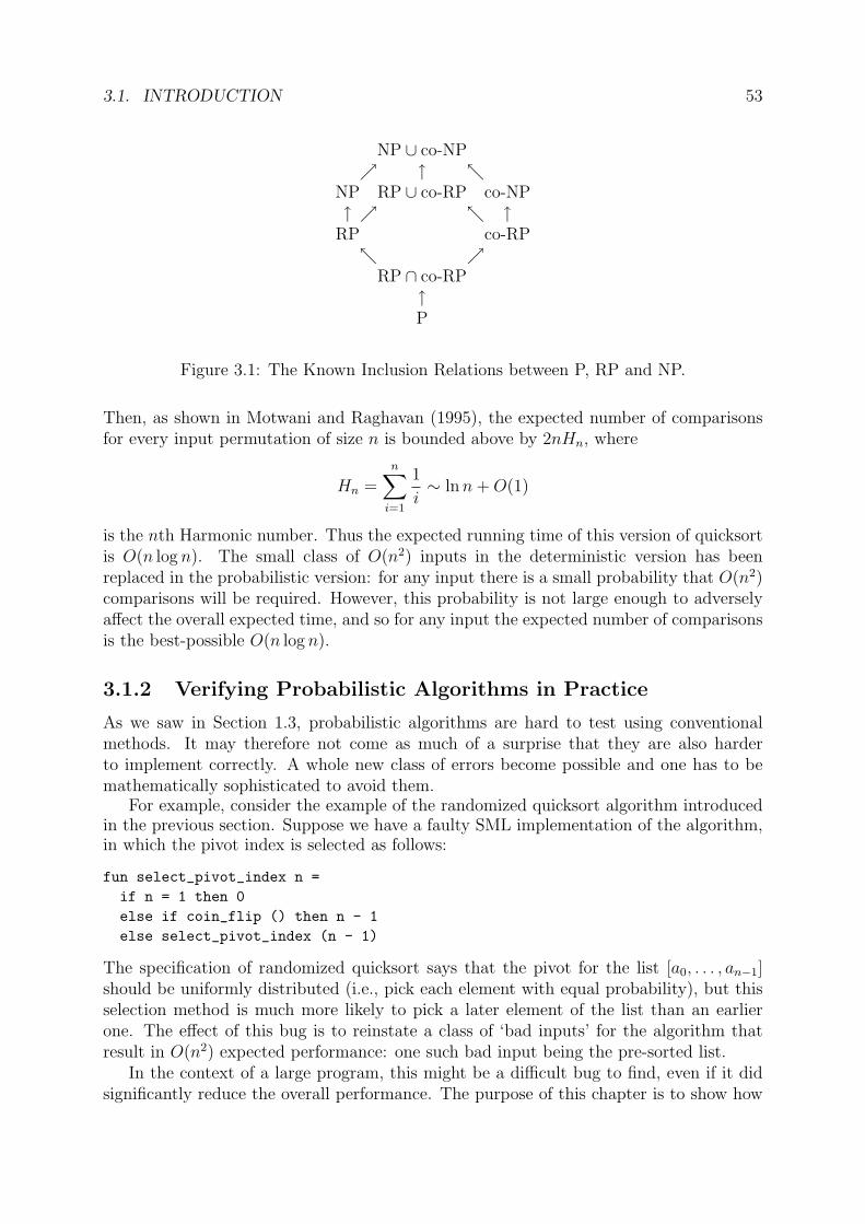
3.1. INTRODUCTION 53
NP ∪ co-NP ↑
NP RP ∪ co-RP co-NP↑ ↑
RP co-RP
RP ∩ co-RP↑P
Figure 3.1: The Known Inclusion Relations between P, RP and NP.
Then, as shown in Motwani and Raghavan (1995), the expected number of comparisonsfor every input permutation of size n is bounded above by 2nHn, where
Hn =n∑
i=1
1
i∼ lnn+O(1)
is the nth Harmonic number. Thus the expected running time of this version of quicksortis O(n log n). The small class of O(n2) inputs in the deterministic version has beenreplaced in the probabilistic version: for any input there is a small probability that O(n2)comparisons will be required. However, this probability is not large enough to adverselyaffect the overall expected time, and so for any input the expected number of comparisonsis the best-possible O(n log n).
3.1.2 Verifying Probabilistic Algorithms in Practice
As we saw in Section 1.3, probabilistic algorithms are hard to test using conventionalmethods. It may therefore not come as much of a surprise that they are also harderto implement correctly. A whole new class of errors become possible and one has to bemathematically sophisticated to avoid them.
For example, consider the example of the randomized quicksort algorithm introducedin the previous section. Suppose we have a faulty SML implementation of the algorithm,in which the pivot index is selected as follows:
fun select_pivot_index n =if n = 1 then 0else if coin_flip () then n - 1else select_pivot_index (n - 1)
The specification of randomized quicksort says that the pivot for the list [a0, . . . , an−1]should be uniformly distributed (i.e., pick each element with equal probability), but thisselection method is much more likely to pick a later element of the list than an earlierone. The effect of this bug is to reinstate a class of ‘bad inputs’ for the algorithm thatresult in O(n2) expected performance: one such bad input being the pre-sorted list.
In the context of a large program, this might be a difficult bug to find, even if it didsignificantly reduce the overall performance. The purpose of this chapter is to show how

54 CHAPTER 3. VERIFYING PROBABILISTIC ALGORITHMS
formal methods may be applied to probabilistic algorithms, so that we can verify in amechanical theorem prover that a program conforms to a probabilistic specification.
Recall from Section 1.4 that we model a probabilistic ‘function’ f : α→ β with a HOLfunction
f : α→ B∞ → β × B∞
that explicitly passes around the sequence of random bits, using some in the computationand passing back the unused bits. In Chapter 2 we defined the probability space (E ,P)which allows us write specifications for probabilistic algorithms. For example, we canformulate goals in the theorem prover such as
∀n. P s | fst (prob program n s) = failure ≤ 2−n (3.1)
to specify the operation of a certain prob program. In a certain theoretical sense, this solvesthe problem of giving semantics to our modelling of probabilistic programs in higher-orderlogic. However, we are interested in mechanically verifying real probabilistic algorithms,and what is so far missing is a collection of proof techniques to make this as smooth aspossible. Upon attempting a typical verification, two difficulties quickly emerge:
1. Since the probability measure P is only defined on events (i.e., sets in E), mucheffort is spent proving that the sets that arise in verification really are events.
2. Many verification goals reduce to the form
P(A1 ∩ A2 ∩ · · · ∩ An) = P(A1)P(A2) · · ·P(An) (3.2)
where the A1, A2, . . . , An are events produced by ‘probabilistic subroutines’. Thisresult follows from the independence of the events, and so a theory of ‘subroutineindependence’ is required.6
In addition, there is another deficiency with the theory up to this point: we havepresented no syntactic support for expressing probabilistic programs. So far we haveassumed they will be expressed directly in λ-calculus, explicitly passing around the bitsequence. To illustrate why this is not satisfactory, consider the probabilistic program dicewhich returns a number in the set 1, 2, 3, 4, 5, 6 uniformly at random. The probabilisticprogram two dice that uses dice to return the sum of two dice can be expressed in λ-calculus as7
two dice = λ s. let (x, s′)← dice s in(let (y, s′′)← dice s′ in (x+ y, s′′)
)This notation, as well as being rather unwieldy, contains opportunities for mistakes byconfusing the three different versions of the random bit sequence. The ability to expressour probabilistic programs in a cleaner way is not just an aesthetic issue of little logicalsignificance. In fact, it clarifies the theory to the point where we can provide practicalsolutions to the two main verification problems listed above.
6This boils down to ensuring that random bits are never re-used by different subroutines: the side-conditions of the theorems we prove will enforce this property.
7It is true that the definition would be shorter if we had not used the syntactic sugar let v ← x in f vfor (λ v. f v) x. However, this only strengthens our basic point that better notation is required, since theshorter version is even more difficult to comprehend.

3.1. INTRODUCTION 55
3.1.3 A Notation for Probabilistic Programs
A useful observation is that our modelling of probabilistic programs in higher-order logicby ‘passing around the random-number generator’ is how probabilistic programs areroutinely written in pure functional languages such as Haskell8 (Wadler, 1992; Launch-bury and Jones, 1994).9 In fact, probabilistic programs live in the more general state-transforming monad,10 where the state that is transformed is the sequence of randombits. Definition 29 gives the monadic operators, which can be used to combine state-transforming programs with a minimum of notational clutter.
Definition 29 The state-transformer monadic operators unit and bind
` ∀ a, s. unit a s = (a, s) (3.3)
` ∀ f, g, s. bind f g s = let (x, s′)← f(s) in g x s′ (3.4)
unit is used to lift values to the monad, and bind is the monadic analogue of functionapplication.
For example, using unit and bind, our two dice program can be expressed concisely as
two dice = bind dice (λx. bind dice (λ y. unit (x+ y)))
Note that the sequence is never referred to directly, instead the unit and bind operatorspass it around behind the scenes.
In addition to providing an elegant notation in which to express probabilistic programs,unit and bind can be used to test whether a property is compositional on probabilisticprograms.
Definition 30 A property Q : (B∞ → α × B∞) → B is compositional for probabilisticprograms if
1. For every a : α,Q(unit a)
2. For every f : B∞ → α× B∞ and g : α→ B∞ → β × B∞,
Q(f) ∧ (∀ a. Q(g(a))) ⇒ Q(bind f g)
Therefore, by writing our probabilistic programs in state-transformer notation, we canautomatically break down compositional properties on the program to properties on thecomponents. For example, if Q is a compositional property and Q(dice) holds, then sodoes Q(two dice).
In Section 3.2 we investigate the compositionality of the measurability and indepen-dence properties for probabilistic programs. Measurability allows us to deduce that sets
8http://www.haskell.org9With hindsight, it is not surprising that we developed the same model independently, since it is a
natural way to model state in an environment with no global variables.10Monads are a notion from category theory, but happily no knowledge of category theory is required
to use the notation to write probabilistic programs.

56 CHAPTER 3. VERIFYING PROBABILISTIC ALGORITHMS
of sequences defined by probabilistic programs really are events. An example of this isthe set
s | fst (prob program n s) = failurethat was part of the example specification (3.1). This set of sequences is guaranteed tobe an event if prob program is measurable. Independence allows us to decompose goalscontaining the probability of an intersection (such as (3.2) above). The end result is acompositional property of probabilistic programs called indep fn that implies measurabilityand independence.
3.1.4 Probabilistic Termination
Many probabilistic algorithms cannot be guaranteed to terminate on any input sequenceof bits. For example, as we shall see in Section 4.3, no terminating algorithm existsto generate uniform random numbers in the range 0, 1, . . . , n − 1 unless n is a powerof 2. Thus if we insist on guaranteed termination, then even the dice program cannotbe implemented. In practice then, the restriction of guaranteed termination is usuallyrelaxed to allow termination with probability 1. This means that the set of sequencesthat cause a probabilistic program to terminate is an event and has probability 1.
In Section 3.3 we define a probabilistic while operator called prob while, with charac-terizing theorem as shown in Definition 31.
Definition 31 A Probabilistic While Loop
` ∀ c, b. (3.5)
(∀ a. b(a) ∈ indep fn) ∧ prob while terminates c b ⇒∀ a.
prob while c b a ∈ indep fn ∧prob while c b a = if c(a) then bind (b(a)) (prob while c b) else unit a
The b parameter is a probabilistic program to advance the state, and has type α→ B∞ →α × B∞. The c parameter is a deterministic condition on the state that decides whetherto perform another iteration, and has type α→ B.
We also define a prob while terminates condition requiring that for every initial statea, the set of sequences that result in the condition c eventually being false is an eventof probability 1. As Definition 31 shows, this termination condition holding means thatprob while c b preserves the important indep fn property of b.
The prob while operator allows us to define in higher-order logic a large class of prob-abilistic algorithms, and the propagation of the indep fn property allows us to assumeuseful results of measurability and independence for each program in the class. However,in practice it is difficult to verify that a particular probabilistic while loop satisfies itsspecification. This is because the usual proof techniques of program correctness rely oninduction over the termination relation, but a probabilistic while loop is explicitly allowedto run forever on some input sequences (as long as the set of those input sequences hasprobability 0).
We remedy this in Section 3.3.3 by using a version of prob while c b called prob while cut c b ncontaining an extra cut-off parameter n. In the cut-off version, if the condition c is still

3.2. MEASURABILITY AND INDEPENDENCE 57
true after n iterations of b then the loop terminates anyway. It is then possible to provethe theorem that if a property holds for prob while cut c b n with probability 1 (for everyn), then it also holds for prob while c b with probability 1. The benefit of this to veri-fication is that prob while cut c b n is a program that is guaranteed to terminate (in atmost n iterations), so the standard program correctness techniques apply, most usefullyinduction on n. In this way some tricky probabilistic reasoning is reduced to a proof byinduction. An example of this reduction can be found in Section 4.4, in the verificationof a sampling algorithm for the Geometric(1
2) distribution.
3.2 Measurability and Independence
3.2.1 Measurability
Recall from Section 2.2.3 that a function f is measurable F G if preimage f maps sets in Gto sets in F . To demonstrate the practical use of measurability, suppose that f : B∞ →α× B∞ models a probabilistic function, and that
A = x | snd (f x) ∈ B
is a set that appears in the verification, where B is an event (i.e., is a member of E : theset of events of the probability space). If we have that
(snd f) ∈ measurable E E
then we can immediately deduce that A ∈ E , since
A = preimage (snd f) B
In practice, we would like to know that11
(fst f) ∈ measurable E U ∧ (snd f) ∈ measurable E E (3.6)
so that we can additionally deduce that the preimage of any set of results of (the firstcomponent of) f is an event. We extend the definition of measurability to probabilisticprograms by saying that f is measurable if it satisfies property (3.6).
It turns out that property (3.6) is compositional for probabilistic programs, in thesense of Definition 30. It is trivial that unit a is measurable for all a; the difficulty isshowing that bind f g is measurable, given that f : B∞ → α × B∞ is measurable andg(a) : B∞ → β × B∞ is measurable for every a : α.
The task is illustrated in Figure 3.2. We aim to show that
fst bind f g ∈ measurable E UP(β)
11This is the same as requiring that
f ∈ measurable E (U ⊗ E)
where U ⊗ E is the σ-algebra generated by the product sets
A×B | A ∈ U ∧B ∈ E

58 CHAPTER 3. VERIFYING PROBABILISTIC ALGORITHMS
’b’a
EVEV
a
fst o f
fst o g a
snd o f
B
F(a)E(a)
Figure 3.2: Is Measurability Compositional?
and so we take an arbitrary set B ∈ UP(β), and the goal is now to show that
preimage (fst bind f g) B
is an event (i.e., a set in E). For each a : α the set
E(a) = preimage (fst g(a)) B
is an event, by the measurability of g(a). Also, the set
F (a) = preimage (fst f) a ∩ preimage (snd f) (E(a))
is an event, by the measurability of f . Finally, the desired preimage can be written as
preimage (fst bind f g) B =⋃
a∈Uα
F (a)
Now we would like to deduce that any union of events is an event, and be done. Un-fortunately, this property of a σ-algebra is only true for countable unions. A sufficientcondition to carry the result then, is for the range of fst f to be countable, and thisfollows from f being measurable by applying a result of Hansell (1971) in the theory ofnon-separable analytic sets. However, this result would be a difficult one to formalize,and so we instead make progress by strengthening the measurability property.
Definition 32 A function f : B∞ → α× B∞ is strongly measurable if
countable (range (fst f)) ∧ (3.7)
(fst f) ∈ measurable E U ∧ (snd f) ∈ measurable E E
Since countability of range is easily shown to be a compositional property, the aboveargument shows that property (3.7) is compositional for probabilistic programs.

3.2. MEASURABILITY AND INDEPENDENCE 59
3.2.2 Function Independence
Recalling Definition 13 in Section 2.2.4 where we defined independence of both sets andfamilies of sets, we now extend this to independence of a function.
Definition 33 The set of independent functions f : B∞ → α× B∞
` indep function = (3.8)
f |indep families
(image (λA. preimage (fst f) A) UP(α))
(image (λE. preimage (snd f) E) E)
Whereas the measurability of a function f : B∞ → α×B∞ is really only a sanity check,independence corresponds to a very natural property of probabilistic programs. Consideronce more the dice probabilistic program, which returns an element of 1, 2, 3, 4, 5, 6uniformly at random. Define the function pair dice as follows:
pair dice = bind dice (λx. bind dice (λ y. unit (x, y))) (3.9)
Intuitively, we would expect that each of the 36 possible results
(1, 1), (1, 2), (1, 3), (1, 4), (1, 5), (1, 6), (2, 1), . . . , (6, 6)
of pair dice would be equally likely. But this reasoning relies on a subtle assumption ofdice that was not explicitly stated: the returned result (i.e., dice roll) is independent ofthe returned sequence. If this is true then our reasoning is valid, since the second call todice is not biased by the result of the first call. But consider this broken version of dice
broken dice = λ s. (fst (dice s), s)
that always returns the sequence that is passed in. If pair dice had called this instead ofdice, then the independence assumption is not valid, and in fact, only 6 results out of thepossible 36 can occur, namely
(1, 1), (2, 2), (3, 3), (4, 4), (5, 5), (6, 6)
each one having probability 1/6.Independence then, allows us to decompose our probabilistic program, calculate the
distribution of results for each individual subroutine, and then combine them with mul-tiplication to give the distribution of results for the whole program.
Given this intended application for independence to reasoning about probabilisticprograms, it is therefore a pity that the independence property of Definition 33 is notcompositional. It is true that unit a is independent for every a, and also the sequenceoperations12 sdest and scons b can be shown to be independent. But the following counter-example13 proves that bind does not preserve independence:
f = sdest
g = λx. if x then (λ s. (>, scons > s) else (λ s. (⊥, scons ⊥ s))
12Recall from Section 2.3.1 that shd, stl and scons are the sequence analogues of the list operations hd,tl and cons, and also sdest s = (shd s, stl s).
13Thanks to David Preiss for this counterexample.
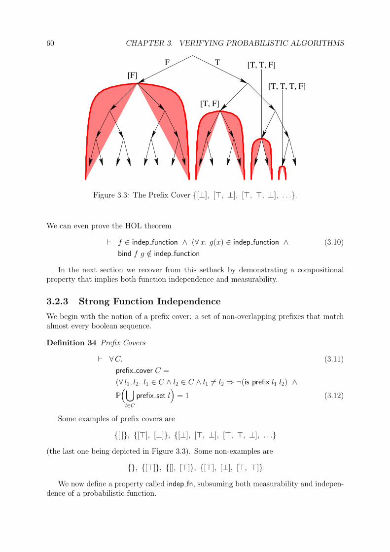
60 CHAPTER 3. VERIFYING PROBABILISTIC ALGORITHMS
[F]
[T, F]
[T, T, F]
[T, T, T, F]
TF
Figure 3.3: The Prefix Cover [⊥], [>, ⊥], [>, >, ⊥], . . ..
We can even prove the HOL theorem
` f ∈ indep function ∧ (∀x. g(x) ∈ indep function ∧ (3.10)
bind f g /∈ indep function
In the next section we recover from this setback by demonstrating a compositionalproperty that implies both function independence and measurability.
3.2.3 Strong Function Independence
We begin with the notion of a prefix cover: a set of non-overlapping prefixes that matchalmost every boolean sequence.
Definition 34 Prefix Covers
` ∀C. (3.11)
prefix cover C =
(∀ l1, l2. l1 ∈ C ∧ l2 ∈ C ∧ l1 6= l2 ⇒ ¬(is prefix l1 l2) ∧
P(⋃
l∈C
prefix set l)
= 1 (3.12)
Some examples of prefix covers are
[ ], [>], [⊥], [⊥], [>, ⊥], [>, >, ⊥], . . .
(the last one being depicted in Figure 3.3). Some non-examples are
, [>], [], [>], [>], [⊥], [>, >]
We now define a property called indep fn, subsuming both measurability and indepen-dence of a probabilistic function.

3.2. MEASURABILITY AND INDEPENDENCE 61
Definition 35 Strong Function Independence
` indep fn = (3.13)
f |countable (range (fst f)) ∧(fst f) ∈ measurable E U ∧ (snd f) ∈ measurable E E ∧∃C.
prefix cover C ∧∀ l, s.l ∈ C ∧ s ∈ prefix set l ⇒f(s) = (fst (f(prefix seq l)), sdrop (length l) s)
Since strong function independence is one of the most important concepts of the thesis,let us take some time to understand its meaning. Firstly, it incorporates the measurabilityproperty discussed in Section 3.2.1, which we showed to be compositional. In addition,it says that there exists a prefix cover C, such that for each l ∈ C the function fst f isconstant on prefix set l, and the function snd f is sdrop (length l). This has a naturalinterpretation when we consider f as a probabilistic program: if f uses some bits fromthe sequence to compute its result, then these bits must be removed from the sequence(using sdrop) before the sequence is passed back.
In an imperative language (such as C) where the random number generator is imple-mented using global state, this property is automatically enforced. Whenever a randombit is asked for, the global state in the random number generator is advanced at thesame time. However, modelling global state with state-transforming monads gives us theextra ability to roll back the state to an earlier time. For some notions of state this maybe useful. But in the case where the state is a random number generator, the abilityto roll back the state is nothing more than an opportunity to shoot oneself in the foot.Probabilistic programs are already hard to reason about, and re-using random numbersintroduces dependencies that tremendously complicate the analysis. An example of thisbad behaviour is the broken dice program of Section 3.2.2: in this case the rolling-back ofthe random number generator produced a dice that always returned the same value!
Insisting that once random bits are used they are always thrown away would seem toimply function independence, because the result sequence can never contain any informa-tion about the result value. In fact, this can be made rigorous, yielding the first propertyof strong function independence:
` indep fn ⊂ indep function (3.14)
Note there is some subtlety here: a function that is indep fn might behave badly onsequences that are not in the prefix cover. However, by the definition of prefix cover, thebad behaviour can only occur inside an event of probability 0, so does not affect the valueof any probabilities.
The second property of strong function independence is that it is not the same asfunction independence. Setting
f = λ s. (shd s = shd (stl s), stl s)

62 CHAPTER 3. VERIFYING PROBABILISTIC ALGORITHMS
we can prove the HOL theorems
` f ∈ indep function (3.15)
` f /∈ indep fn (3.16)
This f is ‘functionally equivalent’ to sdest, returning a (coin-flip) boolean and a sequencethat are independent of each other. The difference is that sdest satisfies strong functionindependence, but f uses two bits from the sequence and only throws one away, violatingthe property.
In practice, restricting ourselves to strongly independent functions does not cause anyproblems. The independent functions that we exclude (such as f) are pathological exam-ples; by definition they cannot be coded in an imperative language with a global randomnumber generator. In addition, as we showed in Section 3.2.2, function independence isnot compositional, so we should expect that some independent functions must be sacri-ficed to make the property compositional. This is the third property of strong functionindependence.
Theorem 36 Strong Function Independence is Compositional
` sdest ∈ indep fn (3.17)
` ∀ a. unit a ∈ indep fn (3.18)
` ∀ f, g. (3.19)
f ∈ indep fn ∧ (∀ a. g(a) ∈ indep fn) ⇒ bind f g ∈ indep fn
Proof: (Sketch) It is easily seen that the prefix cover [>], [⊥] provides the witness forsdest, and similarly [ ] works for every unit a.
Turning our attention to bind: by hypothesis we have a prefix cover F for f , and forevery a we have a prefix cover G(a) for g(a). It can be shown that the set⋃
l∈F
⋃l′∈G(fst (f(prefix seq l))) append l l′
is a prefix cover for bind f g. 2
This says that if we define a function f that accesses the random bit sequence usingonly the sdest, unit and bind primitives, then f is guaranteed to satisfy strong functionindependence. This already includes a significant number of real probabilistic programs,and we shall see in Chapter 5 that it is both possible and desirable to fit the Miller-Rabinprobabilistic primality test into this class.
In addition, there are many properties that are satisfied by every strongly independentfunction, and if proved at this level of abstraction then we can instantiate them to anystrongly independent function that appears in the verification. An example of such aproperty is the following theorem:
` ∀ f1, f2, g1, g2, B. (3.20)
f1 ∈ indep fn ∧ f2 ∈ indep fn ∧(∀ a. g1(a) ∈ indep fn) ∧ (∀ a. g2(a) ∈ indep fn) ∧(∀ a. P s | fst (f1(s)) = a = P s | fst (f2(s)) = a) ∧(∀ a. P s | fst (g1 a s) ∈ B = P s | fst (g2 a s) ∈ B) ⇒P s | fst (bind f1 g1 s) ∈ B = P s | fst (bind f2 g2 s) ∈ B

3.3. PROBABILISTIC TERMINATION 63
From the conditions it is plain that strong function independence is essential to apply thetheorem, which allows us to show that the probability of two bind events can be reducedto the probabilities of their component events. This came in useful during the verificationof the sampling algorithm for the Binomial(n, 1
2) distribution (described in Section 4.2).
3.3 Probabilistic Termination
3.3.1 Probabilistic ‘While’ Loops
We now have all the machinery we need to define a probabilistic ‘while’ loop, where thebody of the while loop is a probabilistic function
b : α→ B∞ → α× B∞
that non-deterministically advances a state of type α, and the condition of the while loopis a deterministic state predicate
c : α→ BWe first define a version of the probabilistic while loop with a cut-off parameter n: if
the condition is still true after n iterations, the loop terminates anyway.
Definition 37 Probabilistic While with a Cut-off
` ∀ c, b, n, a. (3.21)
prob while cut c b 0 a = unit a ∧prob while cut c b (suc n) a =
if c(a) then bind (b(a)) (prob while cut c b n) else unit a
This cut-off version of probabilistic while does not employ probabilistic recursion.Rather it uses standard recursion on the cut-off parameter n, and consequently the fol-lowing properties are easily established by induction on n:
` ∀ c, b, n, a. (3.22)
(∀ a. b(a) ∈ indep fn) ⇒ prob while cut c b n a ∈ indep fn
` ∀ c, b, n, a, p. (3.23)
(∀ a. b(a) ∈ indep fn) ∧ (∀ a. P s | c(fst (b a s)) ≤ p) ⇒P s | c(fst (prob while cut c b n a s)) ≤ pn
` ∀ c, b, n, a. (3.24)
prob while cut c b (suc n) a =
bind (prob while cut c b n a) (λ a′. if c(a′) then b(a′) else unit a′)
We now use prob while cut to make the ‘raw definition’ of prob while
` ∀ c, b, a, s. (3.25)
prob while c b a s =
if ∃n. ¬c(fst (prob while cut c b n a s)) then
prob while cut c b
(minimal (λn. ¬c(fst (prob while cut c b n a s)))) a s
else arb

64 CHAPTER 3. VERIFYING PROBABILISTIC ALGORITHMS
where arb is an arbitrary fixed value. Our goal now is to prove the characterizing theoremof prob while (given in Definition 31).
The first part of the characterizing theorem follows immediately.
Theorem 38
` ∀ c, b, a. (3.26)
prob while c b a = if c(a) then bind (b(a)) (prob while c b) else unit a
Proof: For given values of c, b, a and s, if there is some number of iterations of b(starting in state a with sequence s) that would lead to the condition c becoming false,then prob while performs the minimum number of iterations that are necessary for this tooccur, otherwise it returns arb. The proof now splits into the following cases:
• The condition eventually becomes false:
– The condition is false to start with: in this case the minimum number ofiterations for the condition to become false will be zero.
– The condition is not false to start with: in this case the minimum number ofiterations for the condition to become false will be greater than zero, and sowe can safely perform an iteration and then ask the question again.
• The condition will always be true: therefore, after performing one iteration thecondition will still always be true. So both LHS and RHS are equal to arb.
In each case theorem (3.26) follows. 2
Suppose that for every state a the function b(a) is strongly independent. Therefore,for each a there exists a prefix cover B(a) for the function b(a). Intending C(a) to be aprefix cover for prob while c b a, the family C(a) is defined to be the least fixed point ofthe following rule induction:
¬c(a)
[ ] ∈ C(a)
c(a) ∧ l ∈ B(a) ∧ l′ ∈ C(fst (b a (prefix seq l)))
append l l′ ∈ C(a)
Example: Let the parameters of a probabilistic while loop be
c(a) = a
b(a) = sdest
B(a) = [>], [⊥]
Noting that in our example we have
c(>) ∧ ¬c(⊥) ∧ fst (b a (prefix seq l)) = hd l
let us use the first rule to assign
C(>) = ∅, C(⊥) = [ ]
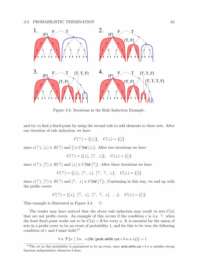
3.3. PROBABILISTIC TERMINATION 65
T T
TT
3.
1. 2.
4.[T, T, T, F]
[F] [F]
[F][T, T, F] [T, T, F]
[F]F
[T, F]
F F
F
[T, F]
[T, F]
Figure 3.4: Iterations in the Rule Induction Example.
and try to find a fixed-point by using the second rule to add elements to these sets. Afterone iteration of rule induction, we have
C(>) = [⊥], C(⊥) = [ ]
since c(>), [⊥] ∈ B(>) and [] ∈ C(hd [⊥]). After two iterations we have
C(>) = [⊥], [>, ⊥], C(⊥) = [ ]
since c(>), [>] ∈ B(>) and [⊥] ∈ C(hd [>]). After three iterations we have
C(>) = [⊥], [>, ⊥], [>, >, ⊥, C(⊥) = [ ]
since c(>), [>] ∈ B(>) and [>, ⊥] ∈ C(hd [>]). Continuing in this way, we end up withthe prefix covers
C(>) = [⊥], [>, ⊥], [>, >, ⊥], . . ., C(⊥) = [ ]
This example is illustrated in Figure 3.4. 2
The reader may have noticed that the above rule induction may result in sets C(a)that are not prefix covers. An example of this occurs if the condition c is λ a. >, whenthe least fixed point works out to be C(a) = ∅ for every a. It is essential for the union ofsets in a prefix cover to be an event of probability 1, and for this to be true the followingcondition of c and b must hold:14
∀ a. P s | ∃n. ¬c(fst (prob while cut c b n a s)) = 1
14The set in this probability is guaranteed to be an event, since prob while cut c b n a satisfies strongfunction independence whenever b does.

66 CHAPTER 3. VERIFYING PROBABILISTIC ALGORITHMS
This is plainly a (probabilistic) termination condition for the while loop, and so we wrapup the property into the following definition, which uses our probabilistic quantifiers(Section 2.4.4).
Definition 39
` ∀ c, b. (3.27)
prob while terminates c b =
∀ a. ∀∗s. ∃n. ¬c(fst (prob while cut c b n a s))
This condition ensures that a prefix cover exists, and therefore that probabilistic whileloops satisfy strong function independence:
` ∀ c, b. (3.28)
(∀ a. b(a) ∈ indep fn) ∧ prob while terminates c b ⇒∀ a. prob while c b a ∈ indep fn
and we have now justified the characterizing theorem of prob while that we gave in Defi-nition 31 (Section 3.1.4).
3.3.2 Probabilistic Termination Conditions
In the previous section we saw that a probabilistic termination condition was needed toprove that a probabilistic while loop satisfied strong function independence. In this sectionwe take a closer look at this condition, in the context of related work on termination.
First, let us consider the deterministic case. As described by Slind (1999), we can usethe HOL function definition package (called TFL) to define a while operator as follows:
while c b a = if c(a) then while c b (b(a)) else a
TFL automatically extracts the termination condition15
∃R. WF R ∧ ∀ a. c(a)⇒ R (b(a)) a
where WF R means that the relation R is well-founded. This is equivalent to16
∀ a. ∃n. ¬c(funpow b n a) (3.29)
which is a deterministic version of our prob while terminates c b condition (Definition 39).It can be easily seen that condition (3.29) is both necessary and sufficient for while c b toterminate on every input a, and a corresponding theorem is true in the probabilistic case.
Theorem 40 The condition prob while terminates c b is both necessary and sufficient foreach prob while c b a to terminate on a set of probability 1.
15Note that TFL must be told to treat this definition as schematic in c and b, or else the extractedtermination condition will be unprovable.
16To see the equivalence, the number n corresponds to the ‘height’ of a in R (well-defined since R iswell-founded).

3.3. PROBABILISTIC TERMINATION 67
Although it is proper for our definition of probabilistic termination to be necessaryand sufficient, in practice it is often easier to show the following simpler condition:
` ∀ c, b. (3.30)
(∀ a. b(a) ∈ indep fn) ∧ (∃∗s. ∀ a. ¬c(fst (b a s))) ⇒prob while terminates c b
This requires an event E with non-zero probability, such that for every state a, if theinput sequence s comes from E then the loop will terminate after one more iteration.
It may seem plausible that we could instead use the condition
∀ a. ∃∗s. ¬c(fst (b a s)))
so that for each state a we could use a different event E(a) (each with non-zero probabil-ity). Unfortunately this does not quite work. A counterexample is the probabilistic whileloop with parameters
c(n, b) = b
b(n, b) = bind (uniform 2n) (λx. (n+ 1, 0 < x))
where uniform n returns a number from the set 0, . . . , n− 1 uniformly at random (Sec-tion 4.3). From the start state (n, b), the (non-zero) probability that the loop will termi-nate after the next iteration is 2−n, but the probability that the loop will ever terminateis
if b then( ∞∑
m=n
2−m)
else 1
which works out to 12
for the start state (2,>).In the context of probabilistic concurrent systems, the following 0-1 law was proved
by Hart et al. (1983):17
Let process P be defined over a state space S, and suppose that from every statein some subset S′ of S the probability of P ’s eventual escape from S′ is at least p,for some fixed 0 < p.
Then P ’s escape from S′ is certain, occurring with probability 1.
Identifying P with prob while c b and S ′ with the set of states a for which c(a) holds, wecan formulate the 0-1 law as an equivalent condition for probabilistic termination:
Theorem 41 The 0-1 Law of Probabilistic Termination
` ∀ c, b. (3.31)
(∀ a. b(a) ∈ indep fn) ⇒(prob while terminates c b ⇐⇒∃ p. 0 < p ∧ ∀ a. p ≤ P s | ∃n. ¬c(fst (prob while cut c b n a s)))
17This paraphrasing comes from Morgan (1996).

68 CHAPTER 3. VERIFYING PROBABILISTIC ALGORITHMS
This interesting result implies that over the whole state space, the infimum of all thetermination probabilities is either 0 or 1, it cannot lie properly in between. To see this,recall that prob while cut c b means that all states terminate with probability 1, but thenegation of the RHS means that there is a state that terminates with probability 0. Anexample of its use for proving probabilistic termination can be found in our verificationof a sampling algorithm for the Bernoulli(p) distribution (Section 4.5).
Hart et al. (1983) also established a sufficient condition for probabilistic terminationcalled the probabilistic variant rule. This has been used by Morgan (1996) to showthe termination of a probabilistic self-stabilization algorithm of Herman (1990). We canformalize this as a sufficient condition for termination of our probabilistic while loops; theproof is relatively easy from the 0-1 law.
Theorem 42 The Probabilistic Variant Condition
` ∀ c, b. (3.32)
(∀ a. b(a) ∈ indep fn) ∧(∃ f,N, p.
0 < p ∧∀ a. c(a) ⇒ f(a) < N ∧ p ≤ P s | f(fst (b a s)) < f(a)) ⇒
prob while terminates c b
As its name suggests, the probabilistic variant condition is a probabilistic analogue ofthe variant method used to prove termination of deterministic while loops. If we can assignto each state a a natural number measure from a finite set, and if each iteration of theloop has probability at least p of decreasing the measure, then probabilistic terminationis assured. In addition, when a | c(a) is finite, condition (3.32) has been shown to benecessary as well as sufficient.
3.3.3 Proof Techniques for Probabilistic While Loops
In this section we consider how to prove some properties of probabilistic while loops thattypically arise in verification. From the way we defined prob while we know that it satisfiesstrong function independence when it can be shown to terminate, and the mechanics ofdoing that were covered in the previous section. However, it turns out to be difficult inpractice to show basic properties that are not immediate consequences of strong functionindependence.
Consider the following program G that lies at the heart of the Geometric(12) sampling
algorithm (Section 4.4):
C = λ (a,m). a
B = λ (a,m). bind sdest (λ a′. unit (a′,m+ 1))
G = prob while C B
The plausible property that G never decreases the second component of the state
∀ a,m, s. m ≤ snd (G (a,m) s)

3.3. PROBABILISTIC TERMINATION 69
is not provable. The reason is that there may be sequences (in this case (>,>, . . .) is theonly example) on which G does not terminate, and so nothing can be said of its result.The correct property is
∀ a,m. ∀∗s. m ≤ snd (G (a,m) s)
but even this turns out to be hard to prove. Often when showing program correctnessit is desirable to induct on the termination relation. However, this is not well-foundedfor our probabilistic while loops, which are explicitly allowed to run forever (so long asthe set of sequences on which they terminate has probability 1). Continuing this train ofthought, it sounds reasonable that we might be able to use induction on a terminationrelation to show properties that are true with probability 1, and indeed this is what thefollowing theorem allows us to do.
Theorem 43 Reduction Theorem for Probabilistic While Loops
` ∀φ, c, b, a. (3.33)
(∀ a. b(a) ∈ indep fn) ∧ prob while terminates c b ∧(∀∗s. ∀n.¬c(fst (prob while cut c b n a s))⇒φ(fst (prob while cut c b n a s))) ⇒∀∗s. φ(fst (prob while c b a s))
Proof: The proof uses the following chain of equalities:
1 = P s | ∃n. ¬c(fst (prob while cut c b n a s))
= Ps
∣∣∣∣ ∃n. ¬c(fst (prob while cut c b n a s)) ∧φ(fst (prob while cut c b n a s))
= P
s∣∣∣∣∣∣ ∃n.
φ(fst (prob while c b a s)) ∧φ(fst (prob while cut c b n a s)) ∧¬c(fst (prob while cut c b n a s))
= P
s
∣∣∣∣ ∃n. φ(fst (prob while c b a s)) ∧¬c(fst (prob while cut c b n a s))
= P s | φ(fst (prob while c b a s))
The first two and the last two probabilities are proved equal using the ∀∗ lifting theoremof Section 2.4.4. 2
Now we may complete our example by applying the above reduction theorem, sincethe generated subgoal
∀∗s. ∀n.¬c(fst (prob while cut C B n (a,m) s))⇒m ≤ (fst (prob while cut C B n (a,m) s))
is further broken down with an application of the quantifier exchange theorem (2.91) of
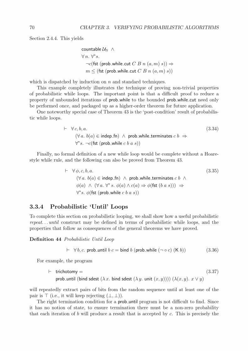
70 CHAPTER 3. VERIFYING PROBABILISTIC ALGORITHMS
Section 2.4.4. This yields
countable UN ∧∀n. ∀∗s.¬c(fst (prob while cut C B n (a,m) s))⇒m ≤ (fst (prob while cut C B n (a,m) s))
which is dispatched by induction on n and standard techniques.This example completely illustrates the technique of proving non-trivial properties
of probabilistic while loops. The important point is that a difficult proof to reduce aproperty of unbounded iterations of prob while to the bounded prob while cut need onlybe performed once, and packaged up as a higher-order theorem for future application.
One noteworthy special case of Theorem 43 is the ‘post-condition’ result of probabilis-tic while loops.
` ∀ c, b, a. (3.34)
(∀ a. b(a) ∈ indep fn) ∧ prob while terminates c b ⇒∀∗s. ¬c(fst (prob while c b a s))
Finally, no formal definition of a new while loop would be complete without a Hoare-style while rule, and the following can also be proved from Theorem 43.
` ∀φ, c, b, a. (3.35)
(∀ a. b(a) ∈ indep fn) ∧ prob while terminates c b ∧φ(a) ∧ (∀ a. ∀∗ s. φ(a) ∧ c(a)⇒ φ(fst (b a s))) ⇒∀∗s. φ(fst (prob while c b a s))
3.3.4 Probabilistic ‘Until’ Loops
To complete this section on probabilistic looping, we shall show how a useful probabilisticrepeat. . . until construct may be defined in terms of probabilistic while loops, and theproperties that follow as consequences of the general theorems we have proved.
Definition 44 Probabilistic Until Loop
` ∀ b, c. prob until b c = bind b (prob while (¬ c) (K b)) (3.36)
For example, the program
` trichotomy = (3.37)
prob until (bind sdest (λx. bind sdest (λ y. unit (x, y)))) (λ(x, y). x ∨ y)
will repeatedly extract pairs of bits from the random sequence until at least one of thepair is > (i.e., it will keep rejecting (⊥,⊥)).
The right termination condition for a prob until program is not difficult to find. Sinceit has no notion of state, to ensure termination there must be a non-zero probabilitythat each iteration of b will produce a result that is accepted by c. This is precisely the
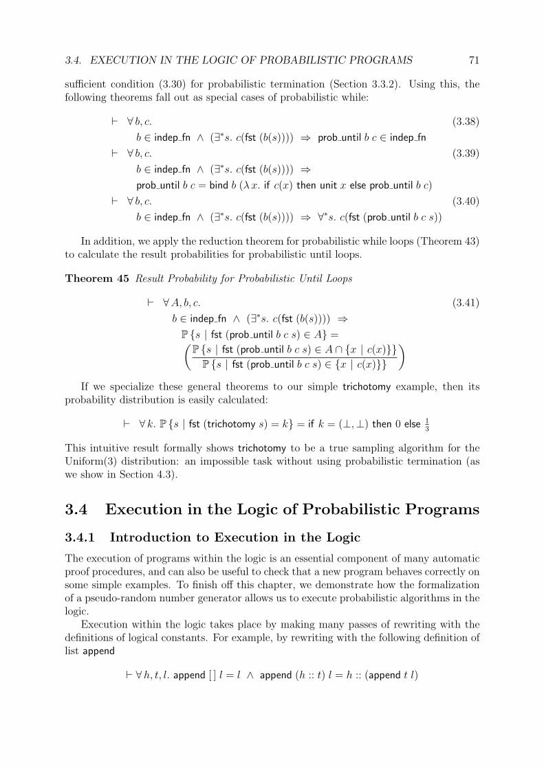
3.4. EXECUTION IN THE LOGIC OF PROBABILISTIC PROGRAMS 71
sufficient condition (3.30) for probabilistic termination (Section 3.3.2). Using this, thefollowing theorems fall out as special cases of probabilistic while:
` ∀ b, c. (3.38)
b ∈ indep fn ∧ (∃∗s. c(fst (b(s)))) ⇒ prob until b c ∈ indep fn
` ∀ b, c. (3.39)
b ∈ indep fn ∧ (∃∗s. c(fst (b(s)))) ⇒prob until b c = bind b (λx. if c(x) then unit x else prob until b c)
` ∀ b, c. (3.40)
b ∈ indep fn ∧ (∃∗s. c(fst (b(s)))) ⇒ ∀∗s. c(fst (prob until b c s))
In addition, we apply the reduction theorem for probabilistic while loops (Theorem 43)to calculate the result probabilities for probabilistic until loops.
Theorem 45 Result Probability for Probabilistic Until Loops
` ∀A, b, c. (3.41)
b ∈ indep fn ∧ (∃∗s. c(fst (b(s)))) ⇒P s | fst (prob until b c s) ∈ A =(
P s | fst (prob until b c s) ∈ A ∩ x | c(x)P s | fst (prob until b c s) ∈ x | c(x)
)If we specialize these general theorems to our simple trichotomy example, then its
probability distribution is easily calculated:
` ∀ k. P s | fst (trichotomy s) = k = if k = (⊥,⊥) then 0 else 13
This intuitive result formally shows trichotomy to be a true sampling algorithm for theUniform(3) distribution: an impossible task without using probabilistic termination (aswe show in Section 4.3).
3.4 Execution in the Logic of Probabilistic Programs
3.4.1 Introduction to Execution in the Logic
The execution of programs within the logic is an essential component of many automaticproof procedures, and can also be useful to check that a new program behaves correctly onsome simple examples. To finish off this chapter, we demonstrate how the formalizationof a pseudo-random number generator allows us to execute probabilistic algorithms in thelogic.
Execution within the logic takes place by making many passes of rewriting with thedefinitions of logical constants. For example, by rewriting with the following definition oflist append
` ∀h, t, l. append [ ] l = l ∧ append (h :: t) l = h :: (append t l)
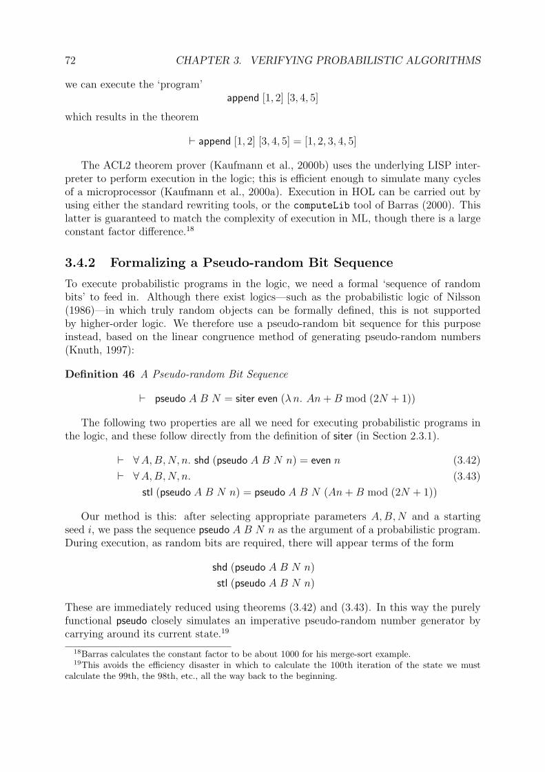
72 CHAPTER 3. VERIFYING PROBABILISTIC ALGORITHMS
we can execute the ‘program’append [1, 2] [3, 4, 5]
which results in the theorem
` append [1, 2] [3, 4, 5] = [1, 2, 3, 4, 5]
The ACL2 theorem prover (Kaufmann et al., 2000b) uses the underlying LISP inter-preter to perform execution in the logic; this is efficient enough to simulate many cyclesof a microprocessor (Kaufmann et al., 2000a). Execution in HOL can be carried out byusing either the standard rewriting tools, or the computeLib tool of Barras (2000). Thislatter is guaranteed to match the complexity of execution in ML, though there is a largeconstant factor difference.18
3.4.2 Formalizing a Pseudo-random Bit Sequence
To execute probabilistic programs in the logic, we need a formal ‘sequence of randombits’ to feed in. Although there exist logics—such as the probabilistic logic of Nilsson(1986)—in which truly random objects can be formally defined, this is not supportedby higher-order logic. We therefore use a pseudo-random bit sequence for this purposeinstead, based on the linear congruence method of generating pseudo-random numbers(Knuth, 1997):
Definition 46 A Pseudo-random Bit Sequence
` pseudo A B N = siter even (λn. An+B mod (2N + 1))
The following two properties are all we need for executing probabilistic programs inthe logic, and these follow directly from the definition of siter (in Section 2.3.1).
` ∀A,B,N, n. shd (pseudo A B N n) = even n (3.42)
` ∀A,B,N, n. (3.43)
stl (pseudo A B N n) = pseudo A B N (An+B mod (2N + 1))
Our method is this: after selecting appropriate parameters A,B,N and a startingseed i, we pass the sequence pseudo A B N n as the argument of a probabilistic program.During execution, as random bits are required, there will appear terms of the form
shd (pseudo A B N n)
stl (pseudo A B N n)
These are immediately reduced using theorems (3.42) and (3.43). In this way the purelyfunctional pseudo closely simulates an imperative pseudo-random number generator bycarrying around its current state.19
18Barras calculates the constant factor to be about 1000 for his merge-sort example.19This avoids the efficiency disaster in which to calculate the 100th iteration of the state we must
calculate the 99th, the 98th, etc., all the way back to the beginning.

3.4. EXECUTION OF PROBABILISTIC PROGRAMS 73
Example: Choosing the parameters
A = 103 B = 95 N = 79
and initial seed 0, we can execute trichotomy in the logic (defined in Section 3.3.4). Thisis performed by using computeLib to rewrite with: the definitions of bind, unit and sdest;the reduction theorems (3.42) and (3.43) above; various boolean simplifications; and thefollowing theorem for trichotomy:
` ∀ s. (3.44)
trichotomy s =
bind sdest
(λx. bind sdest (λ y. if x ∨ y then unit (x, y) else trichotomy)) s
By threading the pseudo-random sequence through many iterations of trichotomy, wecan produce the following chain of theorems:
` trichotomy (pseudo 103 95 75 0) = ((>,⊥), pseudo 103 95 75 65)` trichotomy (pseudo 103 95 75 65) = ((⊥,>), pseudo 103 95 75 33)` trichotomy (pseudo 103 95 75 33) = ((>,⊥), pseudo 103 95 75 94)` trichotomy (pseudo 103 95 75 94) = ((>,⊥), pseudo 103 95 75 107)` trichotomy (pseudo 103 95 75 107) = ((>,>), pseudo 103 95 75 2)` trichotomy (pseudo 103 95 75 2) = ((>,>), pseudo 103 95 75 143)` trichotomy (pseudo 103 95 75 143) = ((⊥,>), pseudo 103 95 75 55)` trichotomy (pseudo 103 95 75 55) = ((⊥,>), pseudo 103 95 75 96)` trichotomy (pseudo 103 95 75 96) = ((>,⊥), pseudo 103 95 75 34)` trichotomy (pseudo 103 95 75 34) = ((>,>), pseudo 103 95 75 32)
etc. . .
2
We emphasize that linear congruential pseudo-random bit sequences are merely aconvenient way to generate superficially unpredictable bits, and are of course completelydeterministic. We might equally well test our probabilistic programs on the sequencewhere every element is >, but this is not even superficially unpredictable. The point iswell made by von Neumann (1963):
Any one who considers arithmetical methods of producing random digits is, ofcourse, in a state of sin. For, as has been pointed out several times, there is no suchthing as a random number—there are only methods to produce random numbers,and a strict arithmetical procedure is of course not such a method.
3.4.3 Execution as an Automatic Proof Procedure
If a deterministic program terminates, the result of the computation will be unique.However, for non-deterministic programs—including probabilistic programs—there maybe many possible results depending on how the internal choices were resolved during thecomputation. Therefore, to get useful results from execution in the logic, we must makeuse of theorems about probabilistic programs that hold for every input sequence of bits.

74 CHAPTER 3. VERIFYING PROBABILISTIC ALGORITHMS
By inspection of the theorems we have proved about probabilistic programs, it looksto be true that programs using probabilistic termination generally have properties thatare quantified by ∀∗ instead of the stronger ∀.20 Here we see a practical effect of this: ∀-quantified theorems apply to every input sequence (and so include our pseudo-random bitsequence), but ∀∗-quantified theorems apply only to an unspecified set of sequences havingprobability 1 (and so might not include our pseudo-random bit sequence). Therefore, weare more likely to be able to deduce useful properties by executing programs in the logicthat do not use probabilistic termination.
For example, consider the following properties of a hypothetical probabilistic program:
∀n. ∀∗s. φ(n) ⇒ ψ(fst (prob program n s)) (3.45)
∀n. ∀ s. φ(n) ⇒ ψ(fst (prob program n s)) (3.46)
Property (3.45) would typically be all that we can prove if prob program employs proba-bilistic termination, whereas the stronger property (3.46) might be provable if prob programdoes not. Suppose we execute
prob program 10 pseudorandom
in the logic for some pseudo-random bit sequence pseudorandom, and in doing so discoverthat
¬ψ(fst (prob program 10 pseudorandom))
With the stronger property (3.46) we can apply the law of contrapositives to deduce thepotentially useful result ¬φ(10), but this does not follow from the weaker property (3.45).
3.5 Concluding Remarks
The main result of this chapter is the development of an infrastructure for the practicalverification of probabilistic algorithms. This builds upon our formalization of probabilitytheory in Chapter 2, and will be applied in Chapters 4 and 5 to verify some exampleprobabilistic programs.
The semantics of probabilistic programs was first tackled by Kozen (1979), and devel-oped by Jones (1990), He et al. (1997) and Morgan et al. (1995). This line of researchextends the predicate transformer idea of Dijkstra (1976) in which programs are regardedas functions: they take a set of desired end results to the set of initial states from whichthe program is guaranteed to produce one of these final states. With the addition ofprobabilistic choice, the ‘sets of states’ must be generalized to functions from states tothe real interval [0, 1]. Jones applies the semantics to proving completeness of a Hoarelogic defined on a little while language equipped with probabilistic choice. It would beinteresting to embed this language in higher-order logic, and use our probability theoryto derive the same proof rules.
The probabilistic dynamic logic of Feldman and Harel (1984) is another extensionof Kozen’s initial work. The essential concepts of their system are the same as ours;programs operate on a sequence of random variables; the analysis is measure-theoretic,
20This is observed to be the case in Section 4.3, where we compare implementations of Uniform(n)sampling algorithms with and without probabilistic termination.

3.5. CONCLUDING REMARKS 75
and cylinders (our prefix sets) play an important role. One difference from our model isthat random variables can come from arbitrary probability distributions, but we provideonly the Bernoulli(1
2) distribution as primitive (others may derived by using sampling
functions). In addition, they support reasoning about partial functions, but lack ourprobabilistic quantifiers. Their resulting logic is a two-level extension of first-order logic,with an axiomatized proof system. Our logic is simpler, by virtue of being a definitionalextension of higher-order logic.
There are many application domains in which it is natural to use continuous distri-butions, and the approach laid out in this chapter adapts very well to algorithms thataccess the continuous distributions using infinite precision real arithmetic. In this way oflooking at things, our infinite sequence of samples from Bernoulli(1
2) is a single sample
from Uniform[0, 1]. Knuth and Yao (1976) show how to use a sequence of random bits toefficiently generate bits of many more continuous distributions, and it would be interestingto verify some simple algorithms along these lines.
Finally, we examine our underlying assumption that probabilistic programs have accessto a source of Bernoulli(1
2) random bits. In terms of whether this is sufficient to model all
probabilistic programs, Gill (1977) showed that the computational power of a languagewith probabilistic choice ∨p is the same as a language with ∨ 1
2, so long as p is computable.
In the other direction, do infinite sequences of IID Bernoulli(12) random variables exist in
the real world? Leaving aside the more difficult independence issues, von Neumann (1963)gives a neat trick to obtain a precisely fair coin (sequence of IID Bernoulli(1
2) random
variables) from any biased coin (sequence of IID Bernoulli(p) random variables21). Flipthe biased coin twice, and if the result is HT then output H, if the result is TH thenoutput T , and if the result is HH or TT then output nothing. Independent of how thecoin is biased, we know that the probability of HT must be equal to the probability ofTH, so if we repeat this procedure long enough then an infinite sequence of fair coin flipswill emerge.
21We must have 0 < p < 1 for this to work.

76 CHAPTER 3. VERIFYING PROBABILISTIC ALGORITHMS

Chapter 4
Example Probabilistic Programs
To illustrate our framework for verifying probabilistic algorithms in a theorem prover, weprove the correctness of several example programs. Most of these are sampling algorithmsfor various probability distributions, which support the development of more sophisticatedprobabilistic programs. We also define the symmetric simple random walk, since it repre-sents a complicated case of probabilistic termination, and verify the ‘optimal dice’ from apaper by Knuth and Yao (1976).
4.1 Introduction
In Chapter 2 we formalized probability theory in higher-order logic, to give meaning tospecifications of probabilistic programs. In Chapter 3 we introduced a convenient notationin which to express implementations of probabilistic programs in higher-order logic. Inaddition, we defined some program constructs (such as prob while) and properties (suchas indep fn) and proved a body of theorems about them. On the strength of all this, weclaimed to have developed a framework in which it was practical to verify probabilisticprograms in a theorem prover. This chapter constitutes evidence substantiating our claim.We implement in higher-order logic several useful probabilistic programs, and formallyverify their correctness.
The probabilistic algorithms that we initially choose to verify are used to generatesamples from different probability distributions, given a source of random bits. Thesesampling algorithms are low-level probabilistic programs, useful in many programmingcontexts where a certain kind of probabilistic behaviour is required. For example, somehardware simulation software may need a particular distribution of inputs to test a circuit,but only has access to random bits from a pseudo-random number generator or from theoperating system.1 Typically, sampling algorithms can be implemented as small proba-bilistic programs, but involve some interesting reasoning about probability to prove theircorrectness. They thus represent ideal examples to test the verification framework we havelaid in place. In addition, once we have verified a suite of sampling algorithms for differ-ent distributions, we can use them as subroutines in higher-level textbook probabilisticalgorithms. Chapter 5 contains a case study where we do just this: using a Uniform(n)
1The latest Verilog standard (IEEE Standards Department, 2001) includes some continuous distribu-tion sampling algorithms for just such a purpose. To further motivate our own work, in one draft of thestandard the χ2 distribution sampling algorithm was found to be wrong!
77
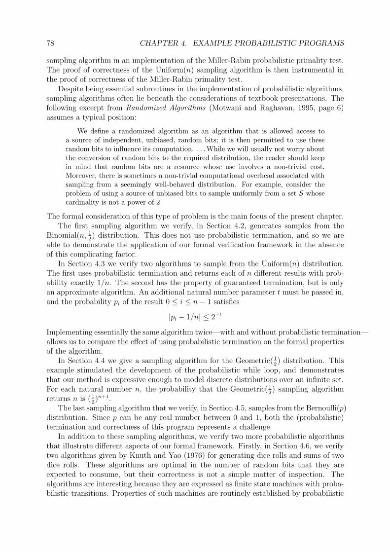
78 CHAPTER 4. EXAMPLE PROBABILISTIC PROGRAMS
sampling algorithm in an implementation of the Miller-Rabin probabilistic primality test.The proof of correctness of the Uniform(n) sampling algorithm is then instrumental inthe proof of correctness of the Miller-Rabin primality test.
Despite being essential subroutines in the implementation of probabilistic algorithms,sampling algorithms often lie beneath the considerations of textbook presentations. Thefollowing excerpt from Randomized Algorithms (Motwani and Raghavan, 1995, page 6)assumes a typical position:
We define a randomized algorithm as an algorithm that is allowed access toa source of independent, unbiased, random bits; it is then permitted to use theserandom bits to influence its computation. . . . While we will usually not worry aboutthe conversion of random bits to the required distribution, the reader should keepin mind that random bits are a resource whose use involves a non-trivial cost.Moreover, there is sometimes a non-trivial computational overhead associated withsampling from a seemingly well-behaved distribution. For example, consider theproblem of using a source of unbiased bits to sample uniformly from a set S whosecardinality is not a power of 2.
The formal consideration of this type of problem is the main focus of the present chapter.The first sampling algorithm we verify, in Section 4.2, generates samples from the
Binomial(n, 12) distribution. This does not use probabilistic termination, and so we are
able to demonstrate the application of our formal verification framework in the absenceof this complicating factor.
In Section 4.3 we verify two algorithms to sample from the Uniform(n) distribution.The first uses probabilistic termination and returns each of n different results with prob-ability exactly 1/n. The second has the property of guaranteed termination, but is onlyan approximate algorithm. An additional natural number parameter t must be passed in,and the probability pi of the result 0 ≤ i ≤ n− 1 satisfies
|pi − 1/n| ≤ 2−t
Implementing essentially the same algorithm twice—with and without probabilistic termination—allows us to compare the effect of using probabilistic termination on the formal propertiesof the algorithm.
In Section 4.4 we give a sampling algorithm for the Geometric(12) distribution. This
example stimulated the development of the probabilistic while loop, and demonstratesthat our method is expressive enough to model discrete distributions over an infinite set.For each natural number n, the probability that the Geometric(1
2) sampling algorithm
returns n is (12)n+1.
The last sampling algorithm that we verify, in Section 4.5, samples from the Bernoulli(p)distribution. Since p can be any real number between 0 and 1, both the (probabilistic)termination and correctness of this program represents a challenge.
In addition to these sampling algorithms, we verify two more probabilistic algorithmsthat illustrate different aspects of our formal framework. Firstly, in Section 4.6, we verifytwo algorithms given by Knuth and Yao (1976) for generating dice rolls and sums of twodice rolls. These algorithms are optimal in the number of random bits that they areexpected to consume, but their correctness is not a simple matter of inspection. Thealgorithms are interesting because they are expressed as finite state machines with proba-bilistic transitions. Properties of such machines are routinely established by probabilistic

4.2. THE BINOMIAL(N, 12) DISTRIBUTION 79
model checkers (such as Prism2), and showing how the verification proceeds in our frame-work sheds light on the connection between the two different methods.
Finally, in Section 4.7, we define a variant of the symmetric simple random walk.Starting at level n, at each step the random walk either moves up a level or down a levelwith probability 1
2each. If it ever hits level 0, then the random walk finishes and returns
the numbers of steps taken. This probabilistic program is interesting because the proofthat it terminates with probability 1 is not at all obvious.
4.2 The Binomial(n, 12) Distribution
The first sampling algorithm we will present samples from the Binomial(n, 12) distribution,
where a Binomial(n, p) random variable is the sum of n independent Bernoulli(p) randomvariables (DeGroot, 1989, page 100). We can thus define a simple sampling algorithm forthe Binomial(n, 1
2) distribution by counting the number of >’s in the first n bits of our
sequence.
Definition 47 The Binomial(n, 12) Sampling Algorithm
` prob binomial 0 = unit 0 ∧ (4.1)
∀n.prob binomial (suc n) =
bind (prob binomial n)
(λm. bind sdest (λ b. unit (if b then suc m else m)))
By induction on n, it is easy to show that this sampling algorithm satisfies strongfunction independence:
` ∀n. prob binomial n ∈ indep fn (4.2)
However, due to an interesting aspect of our definition of prob binomial, it is not quiteso easy to show that it has the correct probability distribution. If we had phrased thedefinition as
. . . prob binomial (suc n) = bind (sdest (λ b. bind (prob binomial n) . . .
so that we extract an element from the sequence and then make the recursive call (insteadof the other way around), then the probability distribution theorem follows by inductionon n. Therefore we proceed using the following bind commutativity theorem to show thatthe two definitions result in events of the same probability:
` ∀ f, g, h, A. (4.3)
f ∈ indep fn ∧ g ∈ indep fn ∧ (∀x, y. h x y ∈ indep fn) ⇒P(preimage (fst bind f (λx. bind g (λ y. h x y))) A) =
P(preimage (fst bind g (λ y. bind f (λx. h x y))) A)
2http://www.cs.bham.ac.uk/~dxp/prism/

80 CHAPTER 4. EXAMPLE PROBABILISTIC PROGRAMS
This is proved using the associativity of bind3 and theorem (3.20) relating the probabilityof two bind events (Section 3.2.3).
Finally, we may deduce that prob binomial has the expected distribution:
` ∀n, r. P s | fst (prob binomial n s) = r =
(n
r
)(12
)n(4.5)
Incidentally, although the Binomial(n, 12) example is particularly easy to sample with
a source of random bits, it is not without intrinsic interest. The central limit theorem(DeGroot, 1989, page 275) implies that for large n, the sampling algorithm
bind (prob binomial n)
(λm. unit
(2m− n√
n
))is a good approximation to the normal distribution with mean 0 and standard deviation 1:the most important distribution in statistics.
4.3 The Uniform(n) Distribution
In this section we are interested in sampling from the Uniform(n) distribution, whichassigns equal probability to each element in the set 0, . . . , n− 1. Supposing n− 1 hask bits, we approach the problem with an algorithm that returns the number representedby the first k random bits.
Definition 48 A Sampling Algorithm for Uniform(2k)
` ∀n. (4.6)
prob unif n =
if n = 0 then unit 0 else
bind (prob unif (n div 2))
(λm. bind sdest (λ b. unit (if b then 2m+ 1 else 2m)))
Since prob unif makes no use of probabilistic termination, the following properties maybe proved by (complete) induction on its argument.
` ∀n. prob unif n ∈ indep fn (4.7)
` ∀n, k. (4.8)
(n = 0 ∧ k = 0) ∨ 2k−1 ≤ n < 2k ⇒∀m. P s | fst (prob unif n s) = m = if m < 2k then 2−k else 0
This says that prob unif n samples from a Uniform(m) distribution, but that m can be upto twice as large as n. Before proceeding to the correct sampling algorithm for Uniform(n),
3This is one of the laws that must be satisfied by all monads:
` ∀ f, g, h. bind f (λ x. bind (g(x)) h) = bind (bind f g) h (4.4)
4.3. THE UNIFORM(N) DISTRIBUTION 81
n
P(n)
Figure 4.1: The Distribution Resulting from broken prob uniform.
it is instructive to consider the following broken version:
broken prob uniform n =
bind (prob unif (n− 1)) (λm. unit (if n ≤ m then m− n else m))
This produces the distribution as shown in Figure 4.1, whereas the ideal distribution iscompletely flat. The numbers close to zero have twice the probability of numbers closeto n− 1, because two results of prob unif n map to the smaller numbers, but only one tothe larger numbers. Now we give the correct version.
Definition 49 A Sampling Algorithm for the Uniform(n) Distribution
` ∀n. (4.9)
prob uniform (suc n) = prob until (prob unif n) (λx. x < suc n)
This prob uniform function uses a probabilistic until loop to repeatedly evaluate prob unif,stopping when prob unif returns a number in the correct range. It is deliberately left un-defined on an argument of zero, since the distribution Uniform(0) is an ill-formed concept.Showing termination is easy, since the probability that prob unif returns 0 is 2−k for somek, and so there is a non-zero probability that the loop will terminate on each iteration.We may therefore apply the general prob until theorems of Section 3.3.4 to deduce thefollowing properties of prob uniform:
` ∀n. prob uniform (suc n) ∈ indep fn (4.10)
` ∀n. ∀∗s. fst (prob uniform (suc n) s) < suc n (4.11)
` ∀n,m. (4.12)
m < n ⇒ P s | fst (prob uniform n s) = m = 1/n
We have proved that prob uniform is a correct sampling algorithm for Uniform(n). Itsuse of probabilistic termination is necessary, since an algorithm that is guaranteed toterminate within N steps can only access N random bits. Therefore if a particular resultis produced in q different configurations of these N bits, then it will have probability q/2N .Since 1/n can be written as q/2N only when n is a power of 2, a sampling algorithm forUniform(n) that is guaranteed to terminate can only exist when n is a power of 2.
However, the downside of using probabilistic termination is that the number of ran-dom bits that will be required cannot be bounded in advance. Since random bits are

82 CHAPTER 4. EXAMPLE PROBABILISTIC PROGRAMS
n
P(n)
Figure 4.2: The Distribution Resulting from prob uniform cut.
not a free resource, this may introduce unacceptable overhead into a calculation. Conse-quently, most random number libraries in programming languages do not generate com-pletely uniform random numbers (see Knuth (1997)), but instead try to reduce any biasto an acceptable level.4 For these reasons, we also give a sampling algorithm for an‘approximately-Uniform(n)’ distribution that is guaranteed to terminate.
Definition 50 An Approximately-Uniform(n) Sampling Algorithm
` ∀ t, n. (4.13)
prob uniform cut 0 (suc n) = unit 0 ∧prob uniform cut (suc t) (suc n) =
bind (prob unif n)
(λm. if n ≤ m then prob uniform cut t (suc n) else unit m)
This prob uniform cut function takes an additional parameter t, and evaluates prob unifat most t times to get a number in the correct range. If this never happens, then itreturns 0. It therefore results in an approximately-uniform distribution that slightlyfavours 0, depicted in Figure 4.2.
Noting that each of the t independent calls to prob unif gives a better than 12
probabilityof returning a number in the correct range, it is possible to prove the following theoremsabout the behaviour of prob uniform cut:
` ∀ t, n. prob uniform cut t (suc n) ∈ indep fn (4.14)
` ∀ t, n, s. fst (prob uniform cut t (suc n) s) < suc n (4.15)
` ∀ t, n,m. (4.16)
m < n ⇒ |P s | fst (prob uniform cut n s) = m − 1/n| ≤ 2−t
It is interesting to compare the two sets of theorems that we can prove about prob uniformand prob uniform cut. Both satisfy strong function independence, a basic result of proba-bilistic programs that allows them to be composed in a tractable way. As we discussed, theversion with probabilistic termination can yield precisely correct probabilities, whereasthe version without can only get arbitrarily close. Theorems (4.11) and (4.15) show the
4When the bias is significantly less than the probability of a machine error, this is certainly acceptablefor all practical purposes.
4.4. THE GEOMETRIC(12) DISTRIBUTION 83
ranges of the two algorithms, but where the ∀∗ quantifier in the theorem for prob uniformsays that the range being correct is an event of probability 1, the corresponding theoremfor prob uniform cut is much stronger: every input sequence gives a result in the correctrange.
The conclusion is that if we can implement an algorithm satisfying a specificationwithout using probabilistic termination, then we can expect it to satisfy stronger proper-ties. In Chapter 5 we exploit this logical consequence of probabilistic termination, slightlytweaking the usual textbook Miller-Rabin algorithm so that it satisfies the same speci-fication, but calls prob uniform cut instead of prob uniform. Our implementation is thenguaranteed to terminate, requires a bounded number of random bits, and satisfies strongversions of some key properties.
4.4 The Geometric(12) Distribution
In any reasonable model of computation with access to a sequence of random bits, only afinite number of bits from the sequence can be read in finite time. Thus in no reasonablemodel of computation will we be able to calculate the function: return the index of thelast > in the sequence, or 0 if there is no last >. Therefore if a distribution has non-zero probability on an infinite number of points, it cannot be modelled without usingprobabilistic termination. Such is the case with the Geometric(1
2) distribution, where a
Geometric(p) random variable is defined to be the index of the first success in an infinitesequence of Bernoulli(p) trials (DeGroot, 1989, page 260). In our model, the Geometric(1
2)
distribution may be sampled by extracting random bits from the sequence, stopping assoon as the first ⊥ is encountered, and returning the number of >’s extracted.
Definition 51 A Sampling Algorithm for the Geometric(12) Distribution
` ∀ b, n. (4.17)
prob geometric iter (b, n) = bind sdest (λ b′. unit (b′, suc n))
` prob geometric = (4.18)
bind (prob while fst prob geometric iter (>, 0)) (λ (b, n). unit (n− 1))
Here the state is a pair, the first component containing the last random bit, and thesecond the number of bits seen so far. This is initialized to (>, 0) and updated by theprobabilistic while loop until the first component becomes ⊥, at which point the result isthe second component (subtracting one because we do not count the final ⊥).
Termination again follows by using the sufficient condition (3.30) established in Sec-tion 3.3.2, and so we may deduce strong function independence:
` prob geometric ∈ indep fn (4.19)
An application of the reduction theorem for while loops (Theorem 43 in Section 3.3.3)allows us to show that prob geometric samples from the correct distribution:
` ∀n. P s | fst (prob geometric s) = n = (12)n+1 (4.20)
In contrast with the theorems we proved about prob uniform, we do not need a theoremabout the range of prob geometric, since the correct range is the entirety of N.

84 CHAPTER 4. EXAMPLE PROBABILISTIC PROGRAMS
4.5 The Bernoulli(p) Distribution
The final distribution that we sample from is the Bernoulli(p) distribution. This dis-tribution is over the boolean values >,⊥, and models a test where > is picked withprobability p and ⊥ with probability 1 − p. Our sequence of random bits each comefrom a Bernoulli(1
2) distribution, and the present goal is to use these to sample from the
Bernoulli(p) distribution, where p is any real number between 0 and 1.5
The sampling algorithm we use is based on a simple intuition. Suppose the binaryexpansion of p is 0.p0p1p2 · · ·, and consider the bits of the random sequence s as forminga binary expansion 0.s0s1s2 · · ·: in this way s can also be regarded as a real numberbetween 0 and 1. Since the ‘number’ s is uniformly distributed between 0 and 1, theprobability that s is less than p is p. Therefore, an algorithm that returns the result >if s is less than p, and ⊥ otherwise, will be sampling from the Bernoulli(p) distribution.This question can be easily decided by looking at the binary expansions, and the matteris further simplified since we can ignore awkward cases (such as s = p) that occur withprobability 0.
Definition 52 A Sampling Algorithm for the Bernoulli(p) Distribution
` ∀ p.prob bernoulli iter p =
bind sdest
(λ b.
unit
(if p < 12
then if b then inl (2p) else inr ⊥else if b then inr > else inl (2p− 1)))
` ∀ p.prob bernoulli p =
bind (prob while is inr (prob bernoulli iter outl) (inl p)) (unit outr)
So that the sampling algorithm implementation fits neatly into a probabilistic whileloop, it makes heavy use of the HOL sum type α+β, having constructors inl, inr, destruc-tors outl, outr and predicates is inl, is inr. However, the intent of the probabilistic whileloop is simply to evaluate s ≤ p by iteration on the bits of s:
• if shd s = ⊥ and 12≤ p, then return >;
• if shd s = > and p ≤ 12, then return ⊥;
• if shd s = ⊥ and p ≤ 12, then repeat with s := stl s and p := 2p;
• if shd s = > and 12≤ p, then repeat with s := stl s and p := 2p− 1.
5The problem for reals is harder than for rationals, since if p = m/n then the following samplingalgorithm trivially works:
bind (prob uniform n) (λ k. unit (k < m))

4.6. OPTIMAL DICE 85
This method of evaluation has two important properties: firstly, it is obviously correctsince the scaling operations on p just have the effect of removing its leading bit; secondly,probabilistic termination holds, since every iteration has a probability 1
2of terminating the
loop. Indeed, Hart’s 0-1 law of termination (Theorem 41) provides a convenient methodof showing probabilistic termination:
` prob while terminates isl (prob bernoulli iter outl) (4.21)
From this follows strong function independence
` ∀ p. prob bernoulli p ∈ indep fn (4.22)
and we can then formulate an alternative definition of prob bernoulli:
` ∀ p. (4.23)
prob bernoulli p =
bind sdest
(λ b.
if b then (if p ≤ 12
then unit ⊥ else prob bernoulli (2p− 1))
else (if p ≤ 12
then prob bernoulli (2p) else unit >))
This definition of prob bernoulli is more readable, closer to the intuitive version, and easierto use in proofs. We use this to prove the correctness theorem:
` ∀ p. 0 ≤ p ∧ p ≤ 1 ⇒ P s | prob bernoulli p s = p (4.24)
The proof of this is quite simple, once the right idea is found. The idea is to show thatthe probability gets within (1
2)n of p, for an arbitrary natural number n. This occurs after
n iterations, as can be shown by induction.It may be slightly counter-intuitive that for any real number 0 ≤ p ≤ 1 we can generate
an event of probability p, using a probabilistic program that with probability 1 will onlylook at a finite number of random bits. However, it might be helpful to look at this in thefollowing way: for any two real numbers 0 ≤ p, q ≤ 1, the probability that prob bernoulli pand prob bernoulli q follow the same execution path is |p− q|. Therefore, for p and q thatdiffer only after position n in their binary expansions, prob bernoulli p and prob bernoulli qwill differ with probability less (1
2)n.
Note that now we have samples from the Bernoulli(p) distribution, it would be simpleto define other standard distributions parameterized by real p. For example, just aswe based our Binomial(n, 1
2) and Geometric(1
2) sampling algorithms on samples from
a Bernoulli(12) distribution, we could similarly define Binomial(n, p) and Geometric(p)
sampling algorithms based on Bernoulli(p) samples.
4.6 Optimal Dice
A paper of Knuth and Yao (1976) shows that many probability distributions can besampled using only a sequence of random bits. One of these is a dice program thatrequires on average 32
3coin flips to produce a dice roll, and this is proved to be optimal.6
The procedure is depicted in Figure 4.3.
6This optimality is very strong: if pn is the probability that the program requires more than n rollsto produce a result, then each pn is minimal over all dice programs.

86 CHAPTER 4. EXAMPLE PROBABILISTIC PROGRAMS
1
2
3
4
5
6
0
Figure 4.3: An Optimal Way to Sample Dice Rolls Using Coin Flips.
The idea is that one starts at the root node and repeatedly tosses a coin, taking a upperbranch whenever the coin produces H, and a lower branch whenever the coin producesT . When a box is reached the procedure is finished, the result being the contents ofthe box. This way of representing probabilistic programs is called a DDG-tree,7 and anyprobabilistic program using a source of random bits can be written as a (possibly infinite)DDG-tree.
We can model finite DDG-trees as HOL probabilistic programs, and then verify thatthey produce the correct probability distribution. The procedure is illustrated on the diceDDG-tree. Starting at the root node (node 0 in Figure 4.3), we make a coin flip to decidewhether to move to node 1 or node 2. Suppose the coin produces a H and so we move tonode 1. Since there is an arrow that returns to node 1 from later in the tree, we declarethis loop with a prob repeat at this point. This means that the nodes after this pointmust return an option type, and the prob repeat construct will repeatedly try the subtreeuntil a some x is returned (it strips off the some using the to create its result). Node 1also contains a coin flip, suppose that another H is produced so that we move to node 3.There is another coin flip here: if it is a H then we return a none to force another tryfrom node 1; and if it is a T then we return some 1. This is the complete model we use,except for the following piece of notational convenience. If we have reached node 4, thenwe know we will never go back to node 1, and so we insert a mmap some so that whateverwe return will automatically be wrapped with a some before it is passed further up thetree.8 We now give the precise definitions of these constructs and the HOL version of the
7DDG stands for Discrete Distribution Generating.8It may be helpful to think of prob repeat as ‘opening a bracket’ that must be closed on every succeeding

4.6. OPTIMAL DICE 87
dice DDG-tree.
Definition 53 Constructs for Modelling DDG-Trees
` ∀ a, b. coin flip a b = bind sdest (λx. if x then a else b) (4.25)
` ∀ a. prob repeat a = mmap the (prob until a is some) (4.26)
` ∀ f,m. mmap f m = bind m (unit f) (4.27)
Definition 54 An Optimal dice Program
` dice = (4.28)
coin flip
(prob repeat
(coin flip
(coin flip (unit none) (unit (some 1)))
(mmap some (coin flip (unit 2) (unit 3))))
(coin flip
(mmap some (coin flip (unit 4) (unit 5)))
(coin flip (unit (some 6)) (unit none))))
Using the techniques we have introduced for verifying probabilistic programs, it ispossible to prove that the dice program returns the right probability distribution:
` ∀n. (4.29)
P s | fst (dice s) = n = if 1 ≤ n ∧ n ≤ 6 then 16
else 0
We now turn our attention to the problem of generating the sum of two dice. Theprobabilistic program
` two dice = bind dice (λ a. bind dice (λ b. unit (a+ b))) (4.30)
will do this, and we can even prove that it returns the right distribution:
` ∀n. (4.31)
P s | fst (two dice s) = n =
if n = 2 ∨ n = 12 then 136
else if n = 3 ∨ n = 11 then 236
else if n = 4 ∨ n = 10 then 336
else if n = 5 ∨ n = 9 then 436
else if n = 6 ∨ n = 8 then 536
else if n = 7 then 636
else 0
Since dice requires on average 323
coin flips, it follows that two dice will require 713. It
might also be thought that since dice was the optimal way to generate a single dice roll,two dice would be the best way to generate the sum of two dice. However, Knuth and Yao(1976) show that this is not so, and in fact the optimal DDG-tree depicted in Figure 4.4requires only 4 7
18coin flips on the average.
branch, either by returning an option type at a leaf node or by inserting an mmap some inside a branch.

88 CHAPTER 4. EXAMPLE PROBABILISTIC PROGRAMS
12
12
9
10
12
10
8
4
6
4
23
4
3 2
2
35
5
5
6
6
8
8
7
7
7
9
9
11
11
11
10
Figure 4.4: An Optimal Way to Sample the Sum of Two Dice Rolls.

4.7. THE SYMMETRIC SIMPLE RANDOM WALK 89
Using our constructs for modelling DDG-trees, we can formalize the optimal DDG-treefor generating the sum of two dice, and even prove that it yields the same probabilitydistribution as the straightforward version two dice we gave above:
` ∀n. (4.32)
P s | fst (optimal two dice s) = n = P s | fst (two dice s) = n
The HOL version of this theory (including the full 77-line definition of optimal two dice)can be found in Appendix C.3.
4.7 The Symmetric Simple Random Walk
For all of the probabilistic while loops we have seen so far, it was fairly easy to prove thatthey terminated with probability 1. All followed from some general scheme of probabilistictermination, such as Hart’s 0-1 law. The purpose of this section is to show an example ofa probabilistic program with a more difficult proof of probabilistic termination.
The symmetric simple random walk is a probabilistic process with a compelling in-tuitive interpretation (for a standard probability perspective, see Stirzaker (1994, page145)). A drunk starts at point n (the pub) and is trying to get to point 0 (home). Un-fortunately, every step he makes from point i is equally likely to take him to point i + 1as it is to take him to point i− 1. The following program simulates the drunk’s passagehome; returning the number of steps that were taken.
Definition 55 A Simulation of the Symmetric Simple Random Walk
` ∀n. (4.33)
random lurch n = bind sdest (λ b. unit (if b then n+ 1 else n− 1))
` ∀ f, b, a, k. (4.34)
prob cost f b (a, k) = bind (b(a)) (λ a′. unit (a′, f(k)))
` ∀n, k. (4.35)
random walk n k =
bind (prob while (λ (n, ). 0 < n) (prob cost suc random lurch) (n, k))
(λ ( , k). unit k)
Why should the random walk always terminate? Firstly, let πi,j the probability thatstarting at point i, the drunk will eventually reach point j. We first formalize the twolemmas πp+i,p = πi,0 and πi,0 = πi
1,0. Therefore if the drunk is guaranteed to reach homefrom a pub at point 1, he will be guaranteed to reach home from a pub at any point. Byexamining a single iteration of the random walk we have
π1,0 = 12π2,0 + 1
2= 1
2π2
1,0 + 12
which rewrites to(π1,0 − 1)2 = 0
90 CHAPTER 4. EXAMPLE PROBABILISTIC PROGRAMS
This completes the proof of probabilistic termination, and as usual strong independenceimmediately follows.
` ∀n, k. random walk n k ∈ indep fn (4.36)
At this point, we may formulate the definition of random walk in a more natural way:
` ∀n, k. (4.37)
random walk n k =
if n = 0 then unit k else
coin flip (random walk (n+1) (k+1)) (random walk (n−1) (k+1))
We have now finished the hard work of defining the random walk as a probabilisticallyterminating program. To demonstrate that once defined it is just as easy to reason aboutas any of our probabilistic programs, we prove a basic property of the random walk.
` ∀n, k. ∀∗ s. even (fst (random walk n k s)) = even (n+ k) (4.38)
Therefore for a pub at point 1001, the drunk is guaranteed to get home eventually, buthe must take an odd number of steps to do so!
We can extract this probabilistic program to ML, and repeatedly simulate it usinghigh-quality random bits from the operating system.9 Here is a typical sequence of resultsfrom random walks starting at level 1:
57, 1, 7, 173, 5, 49, 1, 3, 1, 11, 9, 9, 1, 1, 1547, 27, 3, 1, 1, 1, . . .
As can be seen, the number of steps that are required for the random walk to hit zerois usually less than 100. But sometimes, the number can be much larger. Continuingthe above sequence of simulations, the 34th simulation sets a new record of 2645 steps,and the next record-breakers are the 135th simulation with 603787 steps and the 664thsimulation with 1605511 steps. Such large records early on are understandable, since thetheoretical expected number of steps for the random walk is actually infinite!10
4.8 Concluding Remarks
In this chapter we have demonstrated the practical effectiveness of our framework forverifying probabilistic programs in a theorem prover, set up in Chapters 2 and 3. For this
9See Section 5.4 for more details about such extractions.10In case it is difficult to see how an algorithm could have infinite expected running time but terminate
with probability 1, consider an algorithm where the probability of termination after n steps is 6π2n2 . The
probability of termination is then∑n
6π2n2
=6π2
∑n
1n2
=6π2· π
2
6= 1
and the expected running time is ∑n
n6
π2n2=
6π2
∑n
1n
=∞
4.8. CONCLUDING REMARKS 91
purpose we verified a collection of sampling algorithms upon which more sophisticatedprobabilistic programs can be built (such as the Miller-Rabin primality test in Chapter 5),and another two interesting examples of probabilistic programs.
Following our formalization, the correct probabilities for the optimal dice exampleshave also been verified by the Prism probabilistic model checker (Kwiatkowska et al.,2001). The optimal dice programs are naturally expressed as probabilistic finite state au-tomata, and Prism automatically evaluates the final probabilities. It would be interestingto link up a theorem prover and a probabilistic model checker; perhaps some analogue ofbounded model checking could be used to find bugs in probabilistic programs?
Finally, in Section 3.5 we quoted a result of Gill (1977) that “the computational powerof a language with probabilistic choice ∨p is the same as a language with ∨ 1
2, so long as
p is computable.” From our verification of the Bernoulli(p) sampling algorithm, it mayappear that using a source of random bits we can simulate probabilistic choice ∨p for anyp. However, by inspecting the prob bernoulli algorithm, it is only possible to evaluate thealgorithm for a real p that supports the following operations: multiplying by 2; subtractingby 1; comparing with 1
2. Using these operations, we can compute each bit of p, and so
p must be a computable real. Additionally, for every computable p and non-computableq the execution paths of prob bernoulli p and prob bernoulli q will differ with probability|p − q|. Therefore—in line with the result of Gill—prob bernoulli allows us to simulateprobabilistic choice ∨p precisely when p is computable.

92 CHAPTER 4. EXAMPLE PROBABILISTIC PROGRAMS
Chapter 5
Verification of the Miller-RabinPrimality Test
We formally verify a HOL implementation of the Miller-Rabin primality test, a well-known and commercially used probabilistic algorithm. Our fundamental perspective allowsus to define a version with strong properties, which we can execute in the logic to provecompositeness of numbers. Finally, we manually extract the HOL Miller-Rabin test toStandard ML, and its performance is evaluated on a large number of candidate primes.1
5.1 Introduction
5.1.1 The Miller-Rabin Probabilistic Primality Test
In the 1970s a handful of probabilistic algorithms were introduced that demonstratedtwo practical advantages over deterministic alternatives: simplicity of expression andefficiency of execution. An algorithm of Berlekamp (1970) uses randomization to factorpolynomials; Solovay and Strassen (1977) introduced a probabilistic primality test basedon the Jacobi symbol; and Rabin (1976) presented two probabilistic algorithms: the firstfinds the nearest neighbours of a set S ⊂ Rn, and the second uses a number theory resultof Miller (1975) to test numbers for primality.
This last algorithm has subsequently become known as the Miller-Rabin probabilisticprimality test, and is the subject of the present chapter. We implement a version ofthe Miller-Rabin algorithm in HOL, and use our theory of probability to express itsprobabilistic specification. A formalization of Miller’s result is required to show that thealgorithm satisfies its specification, and the verification is completed by using some of theproof techniques for probabilistic programs we developed in Chapter 3.
In his 1976 paper, Rabin evaluated the algorithm by finding the largest prime lessthan 2400 (it took less than a minute to return the result 2400 − 593), and reports that“the algorithm was also used to find twin primes by far larger than any hitherto knownpair.” Today the Miller-Rabin algorithm is used for primality testing in computer algebrasystems such as Mathematica. It is also relevant to public key cryptography software,since the RSA algorithm uses a modulus of the form n = pq where p and q are largeprimes chosen at random. In practice p and q are found by randomly choosing large
1This chapter is a revision of Hurd (2001b).
93

94 CHAPTER 5. THE MILLER-RABIN PRIMALITY TEST
numbers, and then checking them for primality using a convenient primality test such asMiller-Rabin.2
5.1.2 The HOL Verification
The end result of this chapter is a HOL version of the Miller-Rabin probabilistic primalitytest, satisfying the following specification.
Theorem 56 Correctness of the Miller-Rabin Primality Test
` ∀n, t, s. prime n ⇒ fst (miller rabin n t s) = > (5.1)
` ∀n, t. (5.2)
¬prime n ⇒ 1− 2−t ≤ P s | fst (miller rabin n t s) = ⊥
The miller rabin test takes two natural number parameters n and t (in addition to asource s of random bits), where n is the number that we wish to test for primality and tdetermines the amount of computation that the test is allowed to perform. If n is primethen the test is guaranteed to return >; if n is composite then it will return ⊥ withprobability at least 1− 2−t and > with probability at most 2−t. Thus for a given value ofn if miller rabin n t s returns ⊥ then n is definitely composite, but if it returns > then allwe know is that n is probably prime.3 However, setting t = 50 we see that the probabilityof the algorithm returning > for an n that is actually composite is ≤ 2−50 < 10−15.
The novelty of this verification lies in the fact that this is an algorithm with a proba-bilistic specification used in commercial software. In addition, we present in Appendix D aversion of the verified algorithm that we have manually extracted to ML. This is not quiteidentical to the version commonly found in algorithm textbooks, since they assume a gen-erator for the Uniform(n) distribution, while our version works directly from a sequence ofrandom bits. Practically speaking, this makes the textbook version harder to implementproperly, because ‘genuine’ randomness from the operating system is usually presented tothe user as a sequence of random bits. To obtain numbers from a Uniform(n) distribution,a suitable sampling algorithm must be implemented, and we saw in Section 4.3 that thisis a slightly delicate matter.4 In the version we present, a bound can be made on thenumber of random bits that the algorithm will require.
Completing the proof of correctness requires a significant body of group theory andcomputational number theory to be formalized in the theorem prover, and Section 5.2shows how the classical results fit together in the verification. This formalization actuallyconstituted the bulk of the effort and provided the testing ground for a new automaticproof procedure; we briefly report on this experience. Section 5.3 describes the somewhateasier task of interfacing the number theory with the probability theory to produce the
2Surprisingly, the popular email encryption program PGP (and the Gnu version GPG) use the Fermattest to check numbers for primality, although the Miller-Rabin test is stronger and involves no extracomputation.
3Quantifying that ‘probably’ is a hard problem: the probability that n is prime given thatfst (miller rabin n t s) returned > depends on the set S from which n was chosen and the distribu-tion of primes in S.
4An inevitable consequence is the loss of guaranteed termination, replaced with probabilistic termi-nation.

5.2. COMPUTATIONAL NUMBER THEORY 95
result, and we also give an immediate application in the form of a procedure for formallyproving that numbers are composite. Finally, we highlight the software engineering benefitof this formal methods research by manually extracting our Miller-Rabin primality testto the ML programming language. In Section 5.4 we examine the correctness issues inextracting the algorithm to ML, and profile its performance.
5.2 Computational Number Theory
5.2.1 Definitions
Our HOL implementation of the Miller-Rabin algorithm is (almost) a functional trans-lation of the version presented in Cormen, Leiserson, and Rivest (1990). To prepare, wedefine functions to factor out powers of 2 and perform modular exponentiation. Here arethe correctness theorems for these functions:
` ∀n, r, s. (5.3)
0 < n ⇒ (factor twos n = (r, s) ⇐⇒ odd s ∧ 2rs = n)
` ∀n, a, b. 1 < n ⇒ modexp n a b = (ab mod n) (5.4)
Next we define a function witness a n that is completely deterministic, returning > ifthe base a can be used to provide a quick proof that n is composite, and ⊥ otherwise.We assume that a and n satisfy 0 < a < n. The witness function uses a helper functionwitness tail which is defined using pattern-matching.
Definition 57 The Miller-Rabin Witness Function
` ∀n, a, r. (5.5)
witness tail n a 0 = a 6= 1 ∧witness tail n a (suc r) =
let a′ ← a2 mod n
in if a′ = 1 then a 6= 1 ∧ a 6= n− 1 else witness tail n a′ r
` ∀n, a. (5.6)
witness n a =
let (r, s)← factor twos (n− 1) in witness tail n (modexp n a s) r
The witness function calls factor twos to find r, s such that s is odd and 2rs = n − 1,then uses modexp and witness tail to calculate the sequence
(a20s mod n, a21s mod n, . . . , a2rs mod n)
This sequence provides two primality tests for n:
1. a2rs mod n = 1.
2. If a2js mod n = 1 for some 0 < j ≤ r, then either a2j−1s mod n = 1 or a2j−1s mod n =n− 1.
96 CHAPTER 5. THE MILLER-RABIN PRIMALITY TEST
If n is a prime then we wish to show that both these tests will always be true. Test 1 isequivalent to aφ(n) mod n = 1 (since 2rs = n− 1 = φ(n) for n prime), and this is exactlyFermat’s little theorem. For this reason this test for primality is called the Fermat test.Test 2 is true since for every x, if 0 = (x2− 1) mod n = (x+ 1)(x− 1) mod n, then if n isprime we must have that either (x+ 1) mod n = 0 or (x− 1) mod n = 0. We thus obtainthe following correctness theorem for witness:
` ∀n, a. 0 < a < n ∧ witness n a ⇒ ¬prime n (5.7)
5.2.2 Underlying Mathematics
A composite number n that passes a primality test for some base a is called a pseudoprime.In the case of the Fermat test, there exist numbers n that are pseudoprimes for all basesa coprime to n. These numbers are called Carmichael numbers, and the two smallestexamples are 561 and 1729.5 Testing Carmichael numbers for primality using the Fermattest is just as hard as factorizing them, since the only bases that fail the test are multiplesof divisors. Miller’s insight was that by also performing Test 2, the number of bases thatare witnesses for any composite n will be at least (n−1)/2, as formalized in the followingtheorem.6
Theorem 58 Cardinality of Miller-Rabin Witnesses
` ∀n. (5.8)
1 < n ∧ odd n ∧ ¬(prime n) ⇒n− 1 ≤ 2 |a : 0 < a < n ∧ witness n a|
Therefore there are no Carmichael numbers for the Miller-Rabin test, and in fact justpicking bases at random will quickly find a witness. This is the basis for the Miller-Rabinprobabilistic primality test.
We now give a brief sketch of how Theorem 58 is proved, stating which classical resultsof number theory are necessary for the result.
The proof aims to find a proper subgroup B of the multiplicative group Z∗n which
contains all the nonwitnesses. This will then imply the result, since by Lagrange’s theoremthe size of a subgroup must divide the size of the group, and so |B| ≤ |Z∗
n|/2 = φ(n)/2 ≤(n− 1)/2.
Firstly, assume that there exists an x ∈ Z∗n such that xn−1 mod n 6= 1. In this case we
choose B = x ∈ Z∗n : xn−1 mod n = 1. The Fermat test ensures that all nonwitnesses
are members of B, and since B is closed under multiplication it is a proper subgroup ofZ∗
n. Therefore in this case the proof is finished.
51729 is also famous as the Hardy-Ramanujan number, explained by C. P. Snow in the foreword toA Mathematician’s Apology (Hardy, 1993): “Once, in the taxi from London, Hardy noticed its number,1729. He must have thought about it a little because he entered the room where Ramanujan lay inbed and, with scarcely a hello, blurted out his disappointment with it. It was, he declared, ‘rather adull number,’ adding that he hoped that wasn’t a bad omen. ‘No, Hardy,’ said Ramanujan, ‘it is a veryinteresting number. It is the smallest number expressible as the sum of two cubes in two different ways.’ ”(103 + 93 = 1729 = 123 + 13)
6In fact, it is possible to prove a stronger result that the number of nonwitnesses must be at mostφ(n)/4, and furthermore this bound can be attained (an example is the Carmichael number 8911).

5.2. COMPUTATIONAL NUMBER THEORY 97
Secondly, assume that for every x ∈ Z∗n we have that xn−1 mod n = 1. We next show
by contradiction that n cannot be a prime power. If n = pa (with p prime and a > 1), thenZ∗
n is cyclic, and so there exists an element g ∈ Z∗n with order φ(n) = φ(pa) = pa−1(p−1).
But gn−1 mod n = 1, and so pa−1(p−1) | pa−1. This is a contradiction, since p | pa−1(p−1)but p 6 | pa − 1.
Since n is composite but not a prime power, we can find two numbers 1 < a, b withgcd(a, b) = 1 and ab = n. At this point we require the unique r, s such that n− 1 = 2rsand s odd. Next we find a maximal j ∈ 0, . . . , r such that there exists a v ∈ Z∗
n withv2js mod n = n − 1. Such a j must exist, because since s is odd we can set j = 0 andv = n− 1. Now choose
B = x ∈ Z∗n : x2js mod n = 1 ∨ x2js mod n = n− 1
B is closed under multiplication and so is a subgroup of Z∗n; also the maximality of j
ensures that B must contain all nonwitnesses. It remains only to show that B 6= Z∗n. By
the Chinese remainder theorem there exists w ∈ Z∗n such that
w mod a = v mod a ∧ w mod b = 1
and sow2js mod a = a− 1 ∧ w2js mod b = 1
Hence by the Chinese remainder theorem w2js mod n cannot be equal to either 1 or n−1,so w /∈ B and the proof is complete.
5.2.3 Formalization
Formalizing this proof in HOL was a long but mostly routine task, resulting in the theoriesdepicted in Figure 5.1. The most time-consuming activity was a thorough developmentof group theory, from the initial axioms through to classical results such as Lagrange’stheorem (5.9), Fermat’s little theorem for groups (5.10) and the structure theorem forAbelian groups (5.11):
` ∀G ∈ finite group. ∀H ∈ subgroup G. |set H| | |set G| (5.9)
` ∀G ∈ finite group. ∀ g ∈ set G. g|set G| = e (5.10)
` ∀G ∈ finite group. (5.11)
abelian G⇒ ∃ g ∈ set G. ∀h ∈ set G. h|g| = e
This development also allowed some classical arithmetic theorems to be rendered in thelanguage of groups, including the Chinese remainder theorem (5.12) and the existence ofprimitive roots (5.13):
` ∀ p, q. (5.12)
1 < p ∧ 1 < q ∧ gcd p q = 1 ⇒(λx. (x mod p, x mod q)) ∈
group iso (mult group pq)
(prod group (mult group p) (mult group q))
` ∀ p, a. (5.13)
odd p ∧ prime p ∧ 0 < a ⇒ cyclic (mult group pa)

98 CHAPTER 5. THE MILLER-RABIN PRIMALITY TEST
predicate_sets
groups
lists
orders
natural_number_polynomials
arithmetic
finite_groups
binomials
multiplicative_groupsreals
miller_rabin
probability
fundamental_theorem_arithmetic
abelian_groups
miller_rabin_ml
Boxes indicate pre-existing HOL theories, and ellipses are theories created for this devel-opment.
Figure 5.1: The Dependency Relation between the Theories of the HOL Formalization.

5.2. COMPUTATIONAL NUMBER THEORY 99
As well as making the arithmetic theorems more concise, this rendering also allowedthe main proof to proceed entirely in the language of groups, eliminating the burdenof switching mathematical context in the middle of a mechanical proof and incidentallymirroring the informal proof in Section 5.2.2.
The most difficult part of the whole formalization was theorem (5.13), guaranteeingthe existence of primitive roots. This required creating new HOL theories of naturalnumber polynomials and Abelian groups for the a = 1 case, and a subtle argument fromBaker (1984) for the step case.
One surprising difference between the informal mathematics and the formalizationinvolved the use of the fundamental theorem of arithmetic. This states that every nat-ural number can be uniquely factorized into primes, and many informal mathematicalproofs begin by applying this to some variable mentioned in the goal (e.g., by saying “letpa1
1 · · · pakk be the prime factorization of n.”) However, although we had previously formal-
ized the fundamental theorem and it was ready to be applied, in the mechanical proofswe always chose what seemed to be an easier proof direction and so never needed it. Twoexamples of this phenomenon occur in the structure theorem for Abelian groups (5.11),and the cardinality of the witness set (Theorem 58): the former theorem we formalizedusing least common multiples which proves the goal more directly; and in the latter allwe needed was a case split between n being a prime power or being a product of coprimep, q, so we separately proved this lemma.
Finally, this development provided a testing ground for our predicate set prover de-scribed in Appendix B. This automatic proof procedure takes a term t, and derives par-ticular sets S such that t ∈ S can be proved in the current logical context. The procedureworks by first recursively deriving sets for the subterms ti of t, and then using this infor-mation to derive sets for the term t. For example, consider the set P = m : N | 0 < m,where the following theorems allow membership t ∈ P to be deduced from knowledge ofti ∈ P :
` t1 ∈ P ∨ t2 ∈ P ⇒ t1 + t2 ∈ P` t1 ∈ P ∧ t2 ∈ P ⇒ t1t2 ∈ P
So, for instance,
m ∈ P ∨ n ∈ P ∨ p ∈ P ⇒ m+mn+mnp ∈ P
The set membership t ∈ P is clearly equivalent to the property 0 < t, and thereare many more properties that can be phrased more or less directly as set memberships.These include group membership (e.g., g ∗G h ∈ set G) and nonemptiness properties oflists and sets (e.g., l 6= [ ]). The predicate set prover can be used to robustly prove all ofthese simple properties, and these come up time and again as side-conditions that mustbe proved during term rewriting. As a consequence, this new automatic proof procedurelent itself to more efficient development of the theories that needed to be formalized inthis verification, particularly the group theory where almost every theorem has one ormore group membership side-conditions.
If the predicate set prover had not been available, it would have been possible to usethe first-order prover to show most of the side-conditions, but there are three reasonswhy this is a less attractive proposition: firstly it would have required effort to find the
100 CHAPTER 5. THE MILLER-RABIN PRIMALITY TEST
right ‘property propagation’ theorems needed for the each goal; secondly the explicitinvocations would have led to more complicated tactics; and thirdly some of the goalsthat can be proved using our specialized tool would simply have been out of range of amore general first-order prover.
5.3 Probability Theory
5.3.1 Guaranteed Termination
In most algorithm textbooks this is how the Miller-Rabin test is defined:
Given an odd integer n greater than 1, we pick a base a at random from the set1, . . . , n− 1 and call witness n a. Suppose n is composite: since at least (n− 1)/2of the bases in the set are guaranteed to be witnesses, the probability that theprocedure errs is at most ((n− 1)/2) / (n− 1) = 1/2.
This abstract view implicitly assumes a generator of uniform random numbers in therange 0, . . . , n − 1, and would appear to be a natural application for our prob uniformsampling algorithm for the Uniform(n) distribution that we verified in Section 4.3. How-ever, since prob uniform employs probabilistic termination, it is prudent to first considerthe implications of this decision. When input a prime the Miller-Rabin test is alwaysmeant to return > (the only error that is permitted is the return of > for a composite). Ifan implementation of Miller-Rabin employs probabilistic termination then this propertymay be shown to hold with probability 1, but if not then we can prove it for every inputsequence of random bits: a much stronger statement. As well as being a more satisfyingsolution for theoretical reasons, it also confers a practical benefit. We can use our formal-ization of a pseudo-random number generator (Section 3.4) to execute our Miller-Rabintest in the logic: if it returns ⊥ then we can immediately deduce the HOL theorem thatthe input number is composite.
In fact, we can use a single observation to relax the requirement from perfectly uniformrandom numbers to approximately-uniform random numbers, and we may then use thesampling algorithm prob uniform cut that is guaranteed to terminate. The observation isthat the base 1 is always going to be a nonwitness for every n, so to find witnesses we canpick bases from the subset 2, . . . , n − 1. Now if we can guarantee that the probabilityof picking each element from this subset is at least 1/(n − 1), then the probability thatwe pick a witness is still at least (1/(n− 1))((n− 1)/2) = 1/2.
Recall from Chapter 3 that we model probabilistic algorithms as state-transformingfunctions B∞ → α × B∞, where the state models the generator of random bits and hasthe type B∞ of infinite boolean sequences. The probabilistic algorithm prob uniform cuthas an extra parameter t which allows us to specify how close the resulting distributionshould be to the ideal Uniform(n). Its correctness theorem is as follows:
` ∀ t, n, k.k < n ⇒ |P s | fst (prob uniform cut t n s) = k − 1/n| ≤ 2−t
Thus if we use the natural number function log2 that is related to calculating logarithmsto the base 2
` ∀n. log2 n = if n = 0 then 0 else suc (log2 (n div 2)) (5.14)
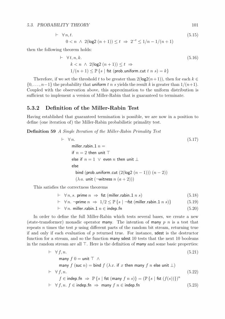
5.3. PROBABILITY THEORY 101
` ∀n, t. (5.15)
0 < n ∧ 2(log2 (n+ 1)) ≤ t ⇒ 2−t ≤ 1/n− 1/(n+ 1)
then the following theorem holds:
` ∀ t, n, k. (5.16)
k < n ∧ 2(log2 (n+ 1)) ≤ t ⇒1/(n+ 1) ≤ P s | fst (prob uniform cut t n s) = k
Therefore, if we set the threshold t to be greater than 2(log2(n+1)), then for each k ∈0, . . . , n−1 the probability that uniform t n s yields the result k is greater than 1/(n+1).Coupled with the observation above, this approximation to the uniform distribution issufficient to implement a version of Miller-Rabin that is guaranteed to terminate.
5.3.2 Definition of the Miller-Rabin Test
Having established that guaranteed termination is possible, we are now in a position todefine (one iteration of) the Miller-Rabin probabilistic primality test.
Definition 59 A Single Iteration of the Miller-Rabin Primality Test
` ∀n. (5.17)
miller rabin 1 n =
if n = 2 then unit >else if n = 1 ∨ even n then unit ⊥else
bind (prob uniform cut (2(log2 (n− 1))) (n− 2))
(λ a. unit (¬witness n (a+ 2)))
This satisfies the correctness theorems
` ∀n, s. prime n ⇒ fst (miller rabin 1 n s) (5.18)
` ∀n. ¬prime n ⇒ 1/2 ≤ P s | ¬fst (miller rabin 1 n s) (5.19)
` ∀n. miller rabin 1 n ∈ indep fn (5.20)
In order to define the full Miller-Rabin which tests several bases, we create a new(state-transformer) monadic operator many. The intention of many p n is a test thatrepeats n times the test p using different parts of the random bit stream, returning trueif and only if each evaluation of p returned true. For instance, sdest is the destructorfunction for a stream, and so the function many sdest 10 tests that the next 10 booleansin the random stream are all >. Here is the definition of many and some basic properties:
` ∀ f, n. (5.21)
many f 0 = unit > ∧many f (suc n) = bind f (λx. if x then many f n else unit ⊥)
` ∀ f, n. (5.22)
f ∈ indep fn ⇒ P s | fst (many f n s) = (P s | fst (f(s)))n
` ∀ f, n. f ∈ indep fn ⇒ many f n ∈ indep fn (5.23)

102 CHAPTER 5. THE MILLER-RABIN PRIMALITY TEST
n Run time GC time
225+ 1 53.080 7.170
226+ 1 370.210 53.530
227+ 1 2842.920 409.620
228+ 1 22095.770 3170.780
Table 5.1: Testing the Composite Prover
Using the new many operator it is simple to define the multiple iteration Miller-Rabintest miller rabin.
Definition 60 The Miller-Rabin Primality Test
` ∀n, t. miller rabin n t = many (miller rabin 1 n) t (5.24)
Finally, the correctness of the Miller-Rabin primality test (Theorem 56) follows from(5.18)–(5.24).
5.3.3 A Compositeness Prover
For any input prime p, Theorem 56 gives us a very strong guarantee: for any t and anysequence s, our implementation of the Miller-Rabin test will always output >. Therefore,given a number n and a sequence s, if execution of miller rabin n 1 s gives the result ⊥,then we can immediately deduce the HOL theorem ` ¬prime n.
Section 3.4 gives us all the machinery we need to execute the Miller-Rabin test insidethe HOL logic.7 Table 5.1 gives the run times in seconds (including garbage collection(GC) time) that was taken to prove the compositeness of some Fermat numbers.
The last number in this table has 78 digits, and demonstrates the possibility of formallyproving numbers to be composite with no knowledge of their factors. Since this proofprocedure is not the main focus of this chapter (rather an interesting digression), we shallnot do any more profiling than this. However, one point that can be made from theexisting results is that from each line of the table to the next, the number of digits in nroughly doubles while the run time increases by a factor of 8. This cubic growth is indeedwhat we would expect if we executed the algorithm in ML, contributing more empiricalevidence to the theoretical result that the efficiency of computeLib is a constant factoraway from ML.
5.4 Extraction to Standard ML
The advantage of extracting the algorithm to a standard programming language such asML is twofold: firstly execution is more efficient, and so the algorithm can be applied tousefully large numbers; and secondly it can be packaged up as a module and used as areliable component of larger programs.
7We use the linear congruence pseudo-random bit generator, with parameters A = 103, B = 95 andN = 79.

5.4. EXTRACTION TO STANDARD ML 103
However, there is a danger that the properties that have been verified in the theo-rem prover are no longer true in the new context. In this section we make a detailedexamination of the following places where the change in context might potentially leadto problems: the source of random bits, the arbitrarily large natural numbers, and themanual translation of the Miller-Rabin functions to ML. Finally we test the algorithm onsome examples, to check again that nothing has gone amiss and also to get some idea ofthe performance and computational complexity of the code.
5.4.1 Random Bits
Our theorems are founded on the assumption that our algorithms have access to a gen-erator of perfectly random bits: each bit has probability of exactly 1
2of being either 1
or 0, and is completely independent of every other bit. In the real world this idealizedgenerator cannot exist, and we must necessarily select an approximation.
The first idea that might be considered is to use a pseudo-random number genera-tor, such as the linear congruence method we used to execute the Miller-Rabin test in thelogic. These have been extensively analysed (for example by Knuth (1997)) and pass manystatistical tests for randomness, but their determinism makes them unsuitable for applica-tions that require genuine unpredictability. For instance, when generating cryptographickeys it is not sufficient that the bits appear random, they must be truly unpredictableeven by an adversary intent on exploiting the random number generator used.
Rejecting determinism, we must turn to the operating system for help. Many modernoperating systems can utilize genuine non-determinism in the hardware to provide a higherquality of random bits. For example, here is a description of how random bits are derivedand made available in Linux, excerpted from the relevant man page:
“The random number generator gathers environmental noise from device driversand other sources into an entropy pool. The generator also keeps an estimate of thenumber of bit[s] of the noise in the entropy pool. From this entropy pool randomnumbers are created.
When read, the /dev/random device will only return random bytes within theestimated number of bits of noise in the entropy pool. /dev/random should besuitable for uses that need very high quality randomness such as one-time pad orkey generation. When the entropy pool is empty, reads to /dev/random will blockuntil additional environmental noise is gathered.
When read, /dev/urandom device will return as many bytes as are requested.As a result, if there is not sufficient entropy in the entropy pool, the returned valuesare theoretically vulnerable to a cryptographic attack on the algorithms used by thedriver. Knowledge of how to do this is not available in the current non-classifiedliterature, but it is theoretically possible that such an attack may exist. If this is aconcern in your application, use /dev/random instead.”
These devices represent the highest quality source of randomness to which we have easyaccess, and so we have packaged them up as ML boolean streams for use in our extractedprogram.

104 CHAPTER 5. THE MILLER-RABIN PRIMALITY TEST
5.4.2 Arbitrarily Large Natural Numbers
Another place where there is a potential disparity between HOL and ML regards theirtreatment of numbers. The HOL algorithm operates on the natural numbers 0, 1, 2, . . .,while in ML the primitive type int contains signed numbers in a range depending on themachine architecture.
We resolved this incompatibility by creating the ML module HolNum, which implementsan equality type num of arbitrarily large natural numbers. The Miller-Rabin functions maythen use this type of numbers, and the arithmetic operations will behave exactly as inHOL.
We first implemented our own large number module, written in the purely functionalsubset of ML (and using a word vector representation of numbers). However, this wasfound to be about 100 times slower than the Moscow ML interface to the GNU Multi-Precision library,8 so we switched to this instead.
5.4.3 Extracting from HOL to ML
A further place where errors could creep in is the manual extraction of the Miller-Rabinfunctions from HOL to ML. Consequently we did this in two steps, the first of which wascreating a new HOL theory containing a version of all the functions we wish to extract.For example, in theorem (5.21) the monadic operator many was defined like so
` ∀ f, n.many f 0 = unit > ∧many f (suc n) = bind f (λx. if x then many f n else unit ⊥)
and in this new HOL theory we prove it is equivalent to
` ∀ f, n.many f n =
if n = 0 then unit >else bind f (λx. if x then many f (n− 1) else unit ⊥)
so that we may export it to ML as
fun MANY f n =if n = ZERO then UNIT trueelseBIND f (fn x => if x then MANY f (n -- ONE) else UNIT false);
As can be seen here the ML version involves some lexical changes,9 but has preciselythe same parse tree as the intermediate HOL version. This reduces the chance of er-rors introduced by the cut-and-paste operation. To compare the two versions of all thefunctions we use, refer to the HOL theory miller rabin ml and the ML program fileMiller.sml in Appendix D.
8http://www.swox.com/gmp/9For example, ZERO, true and -- are the ML versions of the HOL terms 0, > and −.
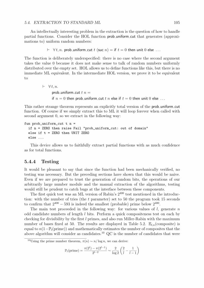
5.4. EXTRACTION TO STANDARD ML 105
An intellectually interesting problem in the extraction is the question of how to handlepartial functions. Consider the HOL function prob uniform cut that generates (approxi-mations to) uniform random numbers:
` ∀ t, n. prob uniform cut t (suc n) = if t = 0 then unit 0 else . . .
The function is deliberately underspecified: there is no case where the second argumenttakes the value 0 because it does not make sense to talk of random numbers uniformlydistributed over the empty set. HOL allows us to define functions like this, but there is noimmediate ML equivalent. In the intermediate HOL version, we prove it to be equivalentto
` ∀ t, n.prob uniform cut t n =
if n = 0 then prob uniform cut t n else if t = 0 then unit 0 else . . .
This rather strange theorem represents an explicitly total version of the prob uniform cutfunction. Of course if we simply extract this to ML it will loop forever when called withsecond argument 0, so we extract in the following way:
fun prob_uniform_cut t n =if n = ZERO then raise Fail "prob_uniform_cut: out of domain"else if t = ZERO then UNIT ZEROelse ...
This device allows us to faithfully extract partial functions with as much confidenceas for total functions.
5.4.4 Testing
It would be pleasant to say that since the function had been mechanically verified, notesting was necessary. But the preceding sections have shown that this would be naive.Even if we are prepared to trust the generation of random bits, the operations of ourarbitrarily large number module and the manual extraction of the algorithms, testingwould still be prudent to catch bugs at the interface between these components.
The first quick test was an ML version of Rabin’s 2400 test mentioned in the introduc-tion: with the number of tries (the t parameter) set to 50 the program took 15 secondsto confirm that 2400 − 593 is indeed the smallest (probable) prime below 2400.
The main test proceeded in the following way: for various values of l, generate nodd candidate numbers of length l bits. Perform a quick compositeness test on each bychecking for divisibility by the first l primes, and also run Miller-Rabin with the maximumnumber of bases fixed at 50. The results are displayed in Table 5.2. El,n(composite) isequal to n(1−Pl(prime)) and mathematically estimates the number of composites that theabove algorithm will consider as candidates.10 QC is the number of candidates that were
10Using the prime number theorem, π(n) ∼ n/ log n, we can derive:
Pl(prime) =π(2l)− π(2l−1)
2l−2∼ 2
log 2
(2l− 1
l − 1
)
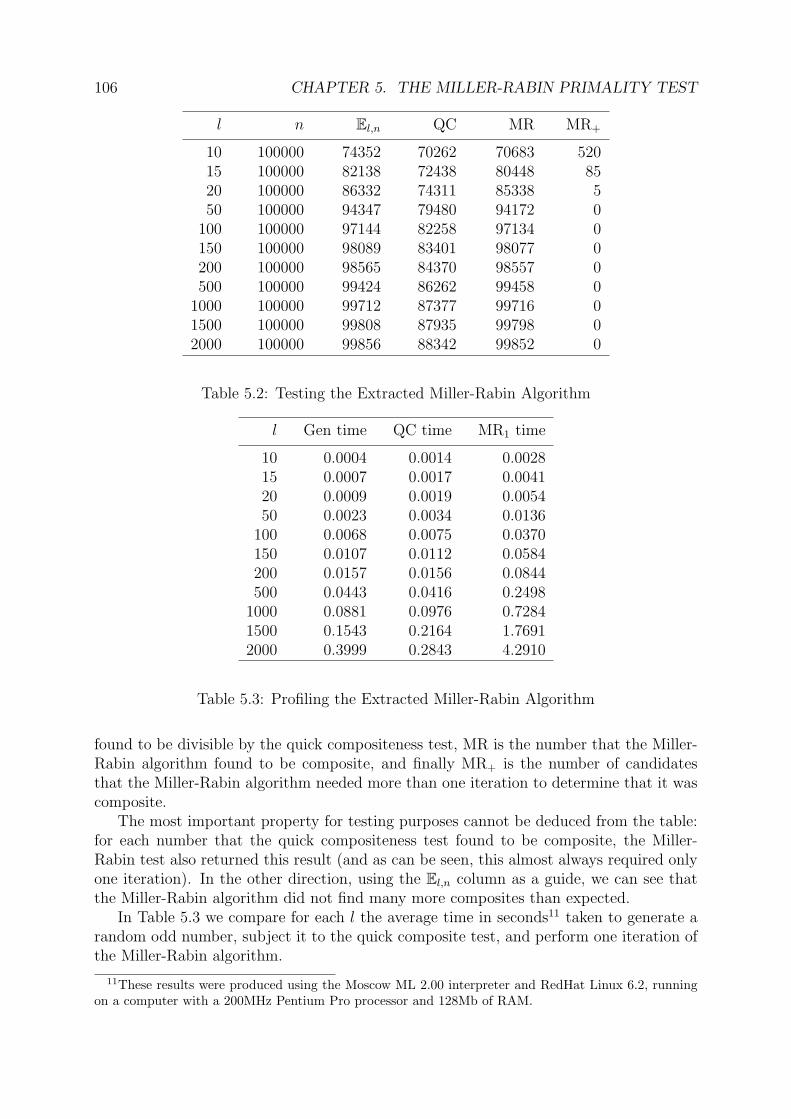
106 CHAPTER 5. THE MILLER-RABIN PRIMALITY TEST
l n El,n QC MR MR+
10 100000 74352 70262 70683 52015 100000 82138 72438 80448 8520 100000 86332 74311 85338 550 100000 94347 79480 94172 0
100 100000 97144 82258 97134 0150 100000 98089 83401 98077 0200 100000 98565 84370 98557 0500 100000 99424 86262 99458 0
1000 100000 99712 87377 99716 01500 100000 99808 87935 99798 02000 100000 99856 88342 99852 0
Table 5.2: Testing the Extracted Miller-Rabin Algorithm
l Gen time QC time MR1 time
10 0.0004 0.0014 0.002815 0.0007 0.0017 0.004120 0.0009 0.0019 0.005450 0.0023 0.0034 0.0136
100 0.0068 0.0075 0.0370150 0.0107 0.0112 0.0584200 0.0157 0.0156 0.0844500 0.0443 0.0416 0.2498
1000 0.0881 0.0976 0.72841500 0.1543 0.2164 1.76912000 0.3999 0.2843 4.2910
Table 5.3: Profiling the Extracted Miller-Rabin Algorithm
found to be divisible by the quick compositeness test, MR is the number that the Miller-Rabin algorithm found to be composite, and finally MR+ is the number of candidatesthat the Miller-Rabin algorithm needed more than one iteration to determine that it wascomposite.
The most important property for testing purposes cannot be deduced from the table:for each number that the quick compositeness test found to be composite, the Miller-Rabin test also returned this result (and as can be seen, this almost always required onlyone iteration). In the other direction, using the El,n column as a guide, we can see thatthe Miller-Rabin algorithm did not find many more composites than expected.
In Table 5.3 we compare for each l the average time in seconds11 taken to generate arandom odd number, subject it to the quick composite test, and perform one iteration ofthe Miller-Rabin algorithm.
11These results were produced using the Moscow ML 2.00 interpreter and RedHat Linux 6.2, runningon a computer with a 200MHz Pentium Pro processor and 128Mb of RAM.

5.5. CONCLUDING REMARKS 107
Figure 5.2: Graph of log(MR1 time) against log l.
The complexity of (one iteration of) the Miller-Rabin algorithm is around O(l2 log l),since it uses asymptotically the same number of operations as modular exponentiation(Cormen et al., 1990). However, performing linear regression on the log-log graph inFigure 5.2 gives a good fit with degree 1.32, implying a complexity of O(l1.32). We canonly conclude that the GNU Multi-Precision library is heavily optimized for the ‘small’numbers in the range we were using, and so we cannot expect an asymptotically validresult.12
5.5 Concluding Remarks
The main result of this chapter is that our framework for verifying probabilistic programsis powerful enough to formally verify the Miller-Rabin primality test in the HOL theoremprover, a well-known and commercially used probabilistic algorithm.
The predicate set prover helped to make the proof development more efficient; it wasparticularly useful for proving group membership conditions and simple but ubiquitousarithmetic conditions. Our evaluation is that it is a useful tool for reasoning about termproperties that naturally propagate up terms, and a useful condition prover for contextualrewriters.
The difference between formal and informal proofs in their use of the fundamental
12Contrast this with the same experiment performed using our own purely functional implementationof arbitrarily large numbers. Linear regression on the log-log graph now gives a good fit with degree 2.98,confirming the theoretical result since we used the simple O(l2) algorithm for multiplication. Incidentally,garbage collection was not the bottleneck in this implementation, typically accounting for less than 5%of the time taken.
108 CHAPTER 5. THE MILLER-RABIN PRIMALITY TEST
theorem of arithmetic was pointed out in Section 5.2.3. This is the most striking exampleof many small differences in the style of informal and formal proofs, stemming from thedifferent proof consumers in each case. Machines make it easier to formalize principlesof induction such as dividing out a prime or prime power factor of a number, whereashumans would seem to be better at reasoning with the multisets that contain the primefactors.
There has been a long history of number theory formalizations, most relevantly forus: a proof of Wilson’s theorem in the Boyer-Moore theorem prover by Russinoff (1985);a correctness proof of the RSA algorithm in ACL2 by Boyer and Moore (1984); and acorrectness proof of RSA in three different theorem provers by Thery (1999). This lastwork was especially useful, since one of the theorem provers was hol98, and we were ableto use his proof of the binomial theorem in our own development.
Though lacking any probabilistic algorithms, the closest work in spirit to this chapteris some recent work on primality proving in Coq by Caprotti and Oostdijk (2001). Theyformalize a similar computational number theory development, and utilize a computeralgebra system to prove numbers prime. Seeing this work improved the organization oftheories in our own formalism. Harrison has also implemented a primality prover in HOL(Light), using Pratt’s criterion instead of Pocklington’s.
Our own development of group theory benefitted from the developments of Gunter(1989), Kammuller and Paulson (1999) and Zammit (1999); the theory of groups hasbeen formalized in many other theorem provers as well.

Chapter 6
Summary
The aim of this thesis has been to show that probabilistic algorithms can be formallyverified using a mechanical theorem prover, ‘just like deterministic algorithms.’
We began in Chapter 2 with an extensive foundational development of probability,creating a higher-order logic formalization of mathematical measure theory. This allowedthe definition of the probability space we use to model a random bit generator, whichinformally is a stream of coin-flips, or technically an infinite sequence of IID Bernoulli(1
2)
random variables. In Chapter 3 we introduced a simple higher-order logic formalismof probabilistic programs, and introduced a probabilistic while loop that allowed us todefine probabilistic programs that terminate with probability 1. Using our formalizedtheory of probability we were able to write specifications for our probabilistic programs,and special emphasis was placed on developing technical support to expedite practicalverification in a mechanical theorem prover. Finally, in Chapter 4 we demonstrated theformal framework with some example probabilistic programs: sampling algorithms forfour probability distributions; some optimal procedures for generating dice rolls from coinflips; the symmetric simple random walk; and in Chapter 5 the Miller-Rabin primalitytest.
This work has made a number of original contributions to knowledge; these werepointed out throughout the text, and here we collect them together in categories andsummarize them:
Probabilistic Algorithms: Our formal framework has allowed us to connect work onsampling probability distributions to textbook presentations of random algorithms.In addition to the theoretical benefits of seeing how the underlying reliance on asource of random bits manifests itself at the level of the random algorithm, we alsoextracted some practical mileage from this connection. Seeing that strong propertiescan be proved of probabilistic programs that avoid probabilistic termination, wedeliberately created a version of the Miller-Rabin primality test that is guaranteedto terminate, and thus for each input an upper bound exists on how many randombits it will require.
Formal Methods: This work has demonstrated that probabilistic algorithms can beverified in a standard theorem prover, and since we have developed our theory as adefinitional extension of higher-order logic, we can have complete confidence in theproperties we prove. Our most significant contributions in this area are: the com-positional property indep fn, showing that all probabilistic programs we construct
109

110 CHAPTER 6. SUMMARY
using our primitives satisfy useful properties of measurability and independence;and the probabilistic while reduction theorem, showing how potentially difficultproofs about probabilistic termination reduce to standard induction techniques. Inaddition, our extraction of the Miller-Rabin primality test gave an example of soft-ware engineering of probabilistic algorithms when a high assurance of correctness isrequired.
Formalized Mathematics: The formalization of mathematics into logic with the aidof mechanical theorem provers is already well-established; indeed the process is vir-tually industrialized in the Mizar theorem prover. In this thesis we have focussed onshowing the utility of such endeavours, by applying formalized theories to the practi-cal task of verifying probabilistic algorithms. Nevertheless, this has necessitated theformalization of some mathematics that has not been previously attempted, suchas Caratheodory’s extension theorem and the construction of a non-measurable setin probability theory, and the existence of primitive roots and the cardinality of theMiller-Rabin witness set in computational number theory. For interest, we presenthere some approximate values for the ‘de Bruijn factor’ (dB)
dB (theorem) =size of textbook proof
size of machine proof
of three textbooks we used:
dB(
Caratheodory’s extension theoremassuming real analysis
)=
4 12 pages of Williams (1991)
1200 proof script lines
dB(
Miller-Rabin witness theoremassuming number theory
)=
1 12 pages of Cormen et al. (1990)
600 proof script lines
dB(
Multiplicative group of pa is cyclicassuming group theory
)=
12 page of Baker (1984)400 proof script lines
Theorem Proving: The investigation (in Appendix B) of PVS predicate subtyping—and showing the extent to which it can be simulated in HOL with predicate sets—provides an interesting comparison of the two theorem provers. One advantage ofworking in an LCF theorem prover is that the ML programming language is providedfor the user to create new proof tools in a secure fashion. Our predicate set proveris a typical example of developing such a tool: automating a particular pattern ofreasoning and then immediately deploying it in our formalization proofs; withoutneeding to worry that soundness may have been violated in some way.
6.1 Future Work
The concluding remarks of each chapter suggested possible improvements and extensionsthat could be made, and so here we consider larger additions to this work.
• Now that we have developed a verification infrastructure, we intend to deploy itin application areas that rely on probabilistic algorithms. Examples include webanonymizing services (such as Crowds (Reiter and Rubin, 1999)) which use prob-abilistic algorithms to prevent web servers from learning information that could

6.1. FUTURE WORK 111
identify their visitors; financial applications which calculate prices of complex bondsusing Monte Carlo integration algorithms (Fishman, 1996); and hardware simula-tors which generate test vectors probabilistically to avoid any bias that may lead tomissing a fault (Bardell et al., 1987).
• Currently the probabilistic programs we verify are expressed as higher-order logicfunctions. It would be possible to formalize in HOL a little while-language contain-ing a probabilistic primitive for obtaining a random bit, and use this to express ourprobabilistic programs. Such a deep embedding would even allow us to capture aclass of strongly independent probabilistic programs in a new HOL type, removingmany side-conditions of theorems.
• Verifying more examples of probabilistic algorithms will inevitably necessitate moreformalization; in particular we already can see that a theory of expectation will berequired to prove the correctness of probabilistic quicksort. If we can continue ourpolicy of formalizing standard theorems of mathematics to aid verifications, thenthis will provide long-term benefits to many users of the HOL theorem prover.
• Proof tools to aid formalization can never be too powerful, and we certainly hadthe impression during our work so far that more could be done to help the user.Although it is difficult to predict exactly where the real benefits will lie in this area,we consider the development of general proof tools to be an important complementto the development of theories.
• Finally, the extraction to ML was an interesting part of the Miller-Rabin verification,and we built from scratch the infrastructure that enabled us to do this. It wouldbe interesting to push this further, perhaps aiming for a whole library of verifiedfunctions built upon some trusted primitives.

112 CHAPTER 6. SUMMARY
Appendix A
Higher-order Logic and the HOLTheorem Prover
This appendix contains a very brief introduction to higher-order logic and its implemen-tation in the HOL theorem prover, containing no more than is necessary for a readerwishing to understand the basis on which this thesis is built. A detailed introduction isgiven by Gordon and Melham (1993) in the canonical reference: Introduction to HOL (Atheorem proving environment for higher order logic).
A.1 Terms and Types
Terms in higher-order logic are typed, and we write t : τ to mean that term t has typeτ . It is helpful to identify types with the set of their elements, so for example the type ofbooleans is B = >,⊥, while the type of natural numbers is N = 0, 1, 2, . . .. Compoundtypes may be created by using type operators; an important example is the function spacetype operator · → ·, so the type N→ B is the set of functions mapping natural numbersto either > or ⊥. Another example is the list type operator ·∗, allowing us to create typessuch as
B∗ = [ ], [>], [⊥], [>,>], . . .Finally, we allow an infinite set α, β, . . . of type variables, which may instantiate toany higher-order logic type. An example of this is the type α∗ of lists containing elementsof type α. This mechanism of polymorphism allows us to prove theorems once about thetype α∗ of lists containing elements of type α, and then instantiate α multiple times togive us the same theorems about B∗, (N→ B)∗, β∗∗ etc.
The terms of higher-order logic are terms of λ-calculus (Church, 1940), where thesyntax λx. t[x] should be read as ‘the function that takes an x and returns t[x].’ The λbinds x, so for example the application of λx. λ x. x to y yields the result λx. x (andnot λx. y). The restriction to typed terms of λ-calculus means that every term must bewell-typed (or inconsistencies emerge in the form of the Russell paradox), where the typerelation is calculated as follows:
Variables: All variables v : τ are well-typed.
Constants: Constants are given a type when they are defined, for example > : B,[ ] : α∗, = : α → α → B and prime : N → B. Any type variables that they contain
113

114 APPENDIX A. HIGHER-ORDER LOGIC AND HOL
may be specialized when they are used in terms, so for example the term [ ] : N∗ iswell-typed.
Function applications: A function term f : α→ β is well-typed when applied to anyargument term x : α, and the result is f(x) : β.
λ-abstractions: Given a variable v : α and a term t[v] : β, the λ-abstraction (λ v. t[v]) :α→ β is well-typed.
Using a type-inference algorithm of Milner (1978), it is possible to take a term t that doesnot contain any type information at all, and deduce a most general type for the term (orraise an error if it is not well-typed). Therefore, when we write terms t : τ of higher-order logic we can safely leave off the type annotation : τ without causing ambiguity. Wegenerally only include type annotations to make things clearer to the reader.
A.2 Theorems
Theorems in higher-order logic are sequents Γ ` t where the term t is the conclusion ofthe theorem, and the set of terms Γ are the hypotheses of the theorem. Typically of LCFtheorem provers, HOL allows the creation of theorems only in the logical kernel, whichfaithfully executes the primitive rules of inference of higher-order logic. For example:
` t = tREFL
Γ ` s = t ∆ ` t = u
Γ ∪∆ ` s = uTRANS
Γ[α] ` t[α]
Γ[σ] ` t[σ]INST TYPE
` (λx. t[x]) u = t[u]BETA CONV
These are four of the primitive rules of inference, asserting that the equality relation isboth reflexive and transitive, that type variables in a theorem may be instantiated to anyhigher-order logic type, and that the usual β-conversion of λ-calculus is valid in higher-order logic. These primitive rules of inference appear in the ML signature of the logicalkernel as follows:
REFL : term→ thm
TRANS : thm→ thm→ thm
INST TYPE : hol type× hol type→ thm→ thm
BETA CONV : term→ thm
Since the ML type thm is abstract, the type security of ML ensures that the functions inthe logical kernel represent the only way that theorems may be created.
A principle of definition implemented as a function in the logical kernel allows newconstants to be defined. Given a theorem1 ` ∃ c : α. P (c), it makes a new constant c : αand returns the characterizing theorem ` P (c). Standard definitions of the form ` c = tare covered in this scheme, since the theorem ` ∃ c. c = t follows trivially by taking thewitness to be t.
To help the reader with the HOL theories in Appendices C and D, in Table A.1 wetabulate the HOL versions of some mathematical symbols we have used.
1For this to be valid, we must insist that P (c) contains no free variables other than c and no typevariables other than those in α.
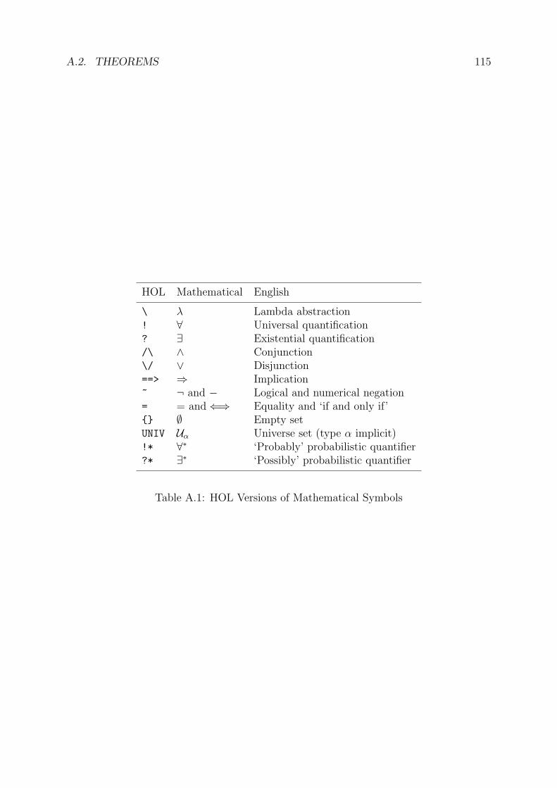
A.2. THEOREMS 115
HOL Mathematical English
\ λ Lambda abstraction! ∀ Universal quantification? ∃ Existential quantification/\ ∧ Conjunction\/ ∨ Disjunction==> ⇒ Implication~ ¬ and − Logical and numerical negation= = and⇐⇒ Equality and ‘if and only if’ ∅ Empty setUNIV Uα Universe set (type α implicit)!* ∀∗ ‘Probably’ probabilistic quantifier?* ∃∗ ‘Possibly’ probabilistic quantifier
Table A.1: HOL Versions of Mathematical Symbols
116 APPENDIX A. HIGHER-ORDER LOGIC AND HOL

Appendix B
Predicate Set Prover
This appendix contains an investigation of predicate subtyping available in the PVS theo-rem prover, and show how it may be simulated in HOL using predicate sets. This leads tothe development of a new proof procedure called the predicate set prover, which employsthis reasoning to prove a class of theorems that frequently appear as side-conditions.1
B.1 Introduction
B.1.1 An Introduction to Predicate Subtyping
PVS (Owre et al., 1999) is an interactive theorem prover implementing a similar logic toHOL; both logics are extensions of the simple type theory of Church (1940). In HOL theextension is Hindley-Milner polymorphism (Milner, 1978), and in PVS it is parametrictheories2 and predicate subtyping (Owre and Shankar, 1997).
Predicate subtyping allows the creation of a new type corresponding to an arbitrarypredicate, where elements of the new type are also elements of the containing type. Asa simple illustration of this, the type of real division (/) in HOL is R → R → R, andin PVS is R → R 6=0 → R, where R is the type of real numbers and R 6=0 is the predicatesubtype of non-zero real numbers, expressed by the predicate λx. x 6= 0.
This extension of the type system allows more information to be encoded in types,leading to benefits for specification and verification such as:
• The ability to express dependent types, for example a type for natural numbersubtraction that prevents the second argument from being larger than the firstargument, or a type representing lists of a fixed length in order to model arrays.
• Greater use of types to express side-conditions of theorems, for example the PVSrewrite rule
`PVS ∀x : R 6=0. x/x = 1 (B.1)
In HOL this would have to be expressed
` ∀x : R. (x 6= 0)⇒ (x/x = 1) (B.2)
1This appendix is a revision of Hurd (2001a).2Parametric theories allow polymorphism at the granularity of the theory (think C++ templates),
whereas Hindley-Milner polymorphism operates at the granularity of the formula (think ML functions).
117
118 APPENDIX B. PREDICATE SET PROVER
and the extra condition must be proved each time the rule is applied.3
• More errors can be found in specifications during type-checking, giving greater con-fidence that the goal is correct before a verification is embarked upon. Mokkedemand Leonard (2000) observed this to be very effective in a large network protocolverification performed in PVS. Many specifications are not verified at all, and inthat case the extra confidence is especially valuable.
However, there are also some costs:
• Type-checking becomes undecidable, so (potentially human) effort must be ex-pended to allow terms to be accepted into the system.
• Type-correctness depends on the current logical context, imposing an extra burdenon term operations to keep careful track of what can be assumed at each subterm.In the case of users wishing to program their own tactics this merely steepens thelearning curve; for term operations in the logical kernel faulty implementations haveproduced a string of soundness bugs.4
In the literature there are papers arguing for and against predicate subtyping. Onthe one hand Shankar and Owre (1999) give many examples of their utility, while on theother Lamport and Paulson (1999) give an example where the costs must be paid withoutmuch benefit, in this case because predicate subtypes cannot naturally encode the desiredinvariant.
B.1.2 Simulating Predicate Subtyping in HOL
In Section B.2 we describe an approach to gain the functionality of predicate subtypes inHOL, without altering the logic in any way. Instead of creating a first-class type associatedwith a particular predicate P , we reason with the subset of elements that satisfy P . Forexample, the PVS predicate subtype R 6=0 can be modelled with the HOL predicate set
nzreal = x : R | x 6= 0
With this substitution, it is possible to assign subtypes to HOL constants, where the PVSsubtype judgement is modelling with a HOL theorem. For example, we assign a subtypeto the real multiplicative inverse (reciprocal) function inv by proving the theorem
` inv ∈ nzreal·→ nzreal
We can even extend this technique to simulate PVS predicate subtype-checking, andpresent an algorithm to derive subtypes for HOL terms. If a term contains violations ofthe subtypes we have assigned, then the algorithm will not be able to derive any subtypesfor the term, and the user is issued a warning about the potential problem. Thus by
3Analogously, typed logics such as HOL and PVS enjoy this advantage over an untyped logic such asZF set theory, in which the theorem ` ∀n : N. n + 0 = n must be expressed ` ∀n. n ∈ N⇒ (n + 0 = n).
4Shankar and Owre (1999) write “these bugs stem largely from minor coding errors rather thanfoundational issues or complexities”. However, the extra complexity generated by predicate subtypingdoes play a part in this: there have been very few soundness bugs found in HOL over the years.
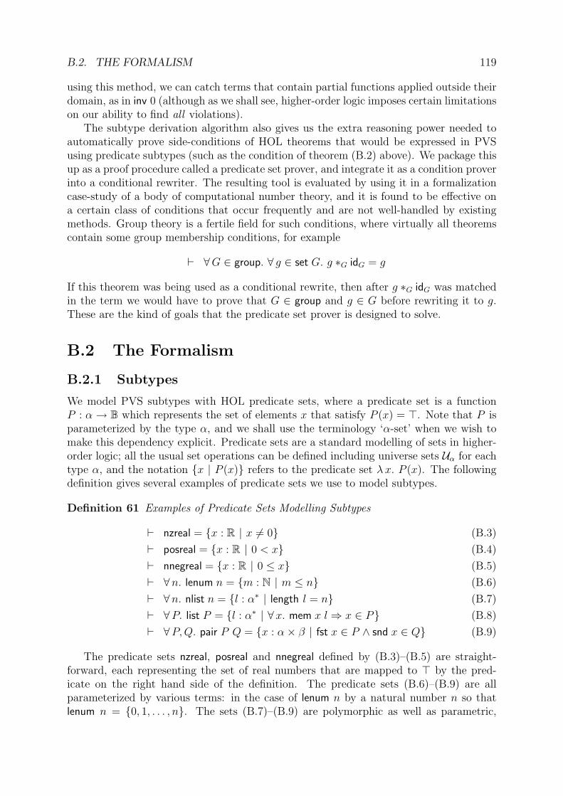
B.2. THE FORMALISM 119
using this method, we can catch terms that contain partial functions applied outside theirdomain, as in inv 0 (although as we shall see, higher-order logic imposes certain limitationson our ability to find all violations).
The subtype derivation algorithm also gives us the extra reasoning power needed toautomatically prove side-conditions of HOL theorems that would be expressed in PVSusing predicate subtypes (such as the condition of theorem (B.2) above). We package thisup as a proof procedure called a predicate set prover, and integrate it as a condition proverinto a conditional rewriter. The resulting tool is evaluated by using it in a formalizationcase-study of a body of computational number theory, and it is found to be effective ona certain class of conditions that occur frequently and are not well-handled by existingmethods. Group theory is a fertile field for such conditions, where virtually all theoremscontain some group membership conditions, for example
` ∀G ∈ group. ∀ g ∈ set G. g ∗G idG = g
If this theorem was being used as a conditional rewrite, then after g ∗G idG was matchedin the term we would have to prove that G ∈ group and g ∈ G before rewriting it to g.These are the kind of goals that the predicate set prover is designed to solve.
B.2 The Formalism
B.2.1 Subtypes
We model PVS subtypes with HOL predicate sets, where a predicate set is a functionP : α→ B which represents the set of elements x that satisfy P (x) = >. Note that P isparameterized by the type α, and we shall use the terminology ‘α-set’ when we wish tomake this dependency explicit. Predicate sets are a standard modelling of sets in higher-order logic; all the usual set operations can be defined including universe sets Uα for eachtype α, and the notation x | P (x) refers to the predicate set λx. P (x). The followingdefinition gives several examples of predicate sets we use to model subtypes.
Definition 61 Examples of Predicate Sets Modelling Subtypes
` nzreal = x : R | x 6= 0 (B.3)
` posreal = x : R | 0 < x (B.4)
` nnegreal = x : R | 0 ≤ x (B.5)
` ∀n. lenum n = m : N | m ≤ n (B.6)
` ∀n. nlist n = l : α∗ | length l = n (B.7)
` ∀P. list P = l : α∗ | ∀x. mem x l⇒ x ∈ P (B.8)
` ∀P,Q. pair P Q = x : α× β | fst x ∈ P ∧ snd x ∈ Q (B.9)
The predicate sets nzreal, posreal and nnegreal defined by (B.3)–(B.5) are straight-forward, each representing the set of real numbers that are mapped to > by the pred-icate on the right hand side of the definition. The predicate sets (B.6)–(B.9) are allparameterized by various terms: in the case of lenum n by a natural number n so thatlenum n = 0, 1, . . . , n. The sets (B.7)–(B.9) are polymorphic as well as parametric,
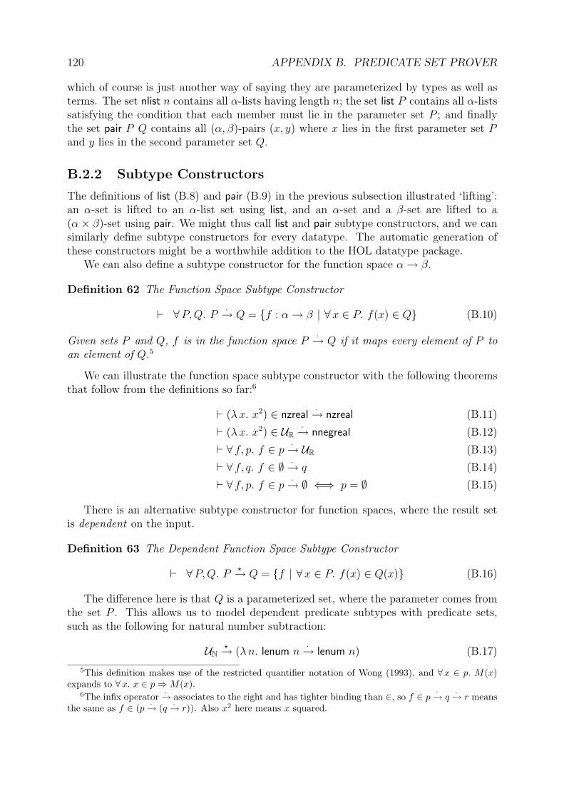
120 APPENDIX B. PREDICATE SET PROVER
which of course is just another way of saying they are parameterized by types as well asterms. The set nlist n contains all α-lists having length n; the set list P contains all α-listssatisfying the condition that each member must lie in the parameter set P ; and finallythe set pair P Q contains all (α, β)-pairs (x, y) where x lies in the first parameter set Pand y lies in the second parameter set Q.
B.2.2 Subtype Constructors
The definitions of list (B.8) and pair (B.9) in the previous subsection illustrated ‘lifting’:an α-set is lifted to an α-list set using list, and an α-set and a β-set are lifted to a(α× β)-set using pair. We might thus call list and pair subtype constructors, and we cansimilarly define subtype constructors for every datatype. The automatic generation ofthese constructors might be a worthwhile addition to the HOL datatype package.
We can also define a subtype constructor for the function space α→ β.
Definition 62 The Function Space Subtype Constructor
` ∀P,Q. P ·→ Q = f : α→ β | ∀x ∈ P. f(x) ∈ Q (B.10)
Given sets P and Q, f is in the function space P·→ Q if it maps every element of P to
an element of Q.5
We can illustrate the function space subtype constructor with the following theoremsthat follow from the definitions so far:6
` (λx. x2) ∈ nzreal·→ nzreal (B.11)
` (λx. x2) ∈ UR·→ nnegreal (B.12)
` ∀ f, p. f ∈ p ·→ UR (B.13)
` ∀ f, q. f ∈ ∅ ·→ q (B.14)
` ∀ f, p. f ∈ p ·→ ∅ ⇐⇒ p = ∅ (B.15)
There is an alternative subtype constructor for function spaces, where the result setis dependent on the input.
Definition 63 The Dependent Function Space Subtype Constructor
` ∀P,Q. P ?→ Q = f | ∀x ∈ P. f(x) ∈ Q(x) (B.16)
The difference here is that Q is a parameterized set, where the parameter comes fromthe set P . This allows us to model dependent predicate subtypes with predicate sets,such as the following for natural number subtraction:
UN?→ (λn. lenum n
·→ lenum n) (B.17)
5This definition makes use of the restricted quantifier notation of Wong (1993), and ∀x ∈ p. M(x)expands to ∀x. x ∈ p⇒M(x).
6The infix operator ·→ associates to the right and has tighter binding than ∈, so f ∈ p·→ q
·→ r meansthe same as f ∈ (p ·→ (q ·→ r)). Also x2 here means x squared.

B.2. THE FORMALISM 121
Recall that UN is the universe set for the type N of natural numbers. We should thereforeread subtype (B.17) above as the set of functions that: given any natural number n returna function from 0, . . . , n to 0, . . . , n. One point to note: if the parameterized set Qhas the form λx. Q′ where Q′ does not contain any occurrences of the bound variable x,then P
?→ Q = P·→ Q′: this shows that Definition 63 is more general than Definition 62.
Dependent types are familiar from type theory, and are incorporated into the LEGOtheorem prover.7
PVS also has two function space subtypes, covering the dependent and non-dependentcases. It also allows dependent products, which we do not use. However, analogouslyto
?→ it is simple to define a dependent pair constructor dpair, taking a set P and aparameterized set Q:
` ∀P,Q. dpair P Q = (x, y) | x ∈ P ∧ y ∈ Q(x) (B.18)
B.2.3 Subtype Rules
Now that we have defined the form of subtype sets, we shall show how to derive subtypesof a HOL term. Given a term t, we say that P is a subtype of t if we can prove thetheorem ` t ∈ P . In our model, these HOL theorems are analogous to PVS subtypejudgements.
The type inference algorithm of Milner (1978) for simply-typed λ-calculus is structural:a single bottom-up pass of a well-formed term suffices to establish its most general type.8
Subtype inference also proceeds by making a single bottom-up pass to derive subtypes,though the new situation is complicated by two factors:
• two rules to break down terms (covering function applications and λ-abstractions)are no longer sufficient, since we also need to keep track of logical context;
• there is no concept of a ‘most general set of subtype theorems’,9 so instead weperform proof search up to some fixed depth and return all the subtype theoremsthat we can prove.
Given a term t, the subtype inference algorithm finds sets P that satisfy t ∈ P . Notethat like the simply-typed λ-calculus, there is essentially no computational differencebetween type inference (i.e., finding P such that t ∈ P holds) and type checking (i.e.,proving t ∈ P for a given P ).
To keep track of logical context, we create subtype rules similar to the congruencerules of a contextual rewriter. Here are some examples:
` ∀ c, a, b, P. (B.19)
(c ∈ UB) ∧ (c⇒ a ∈ P ) ∧ (¬c⇒ b ∈ P )⇒ (if c then a else b) ∈ P` ∀ a, b. (b⇒ a ∈ UB) ∧ (a⇒ b ∈ UB)⇒ (a ∧ b) ∈ UB (B.20)
` ∀ f, a, P,Q. (f ∈ P ?→ Q) ∧ (a ∈ P )⇒ f(a) ∈ Q(a) (B.21)
` ∀ f, P. (∀x. f(x) ∈ P (x))⇒ (λx. f(x)) ∈ (Uα?→ P ) (B.22)
7http://www.dcs.ed.ac.uk/home/lego/8Though not completely avoiding all difficulty: Mairson (1990) has shown that the most general simple
type of a term can be exponentially large in the size of the term.9Theoretically we could intersect all subtypes that a term t satisfies, but then we would just end up
with t if the logical context was consistent, or ∅ if it was not!

122 APPENDIX B. PREDICATE SET PROVER
These rules are rather long, but can be read easily from left to right. For example theconditional subtype rule (B.19) reads: “if we can show c to be in UB; and assuming cwe can show a to be in a subtype P ; and assuming ¬c we can show b to be in the samesubtype P ; then the combined term if c then a else b must also be an element of P .” Inthis way we can build up logical context. Note that c is trivially in the universe set UB,the only purpose of retaining this condition is to force the subtype checker to recurse intoc and check all its subterms. The conjunction rule (B.20) similarly ensures that subtermsare covered by the subtype checker, while building the correct logical context.10 Alsoshown are the subtype rules for function application (B.21) and abstraction (B.22), the
main point to note is that they both use the more general dependent version?→ of the
subtype constructor for function spaces.For each boolean constant , we need a subtype rule of the above form. Therefore the
set of subtype rules used is not fixed; we allow the user to add rules for new constants.Subtype rules tell us how to derive subtypes for a term by combining the subtypes of
smaller terms, but they leave two questions unanswered: how to calculate the subtypesof base terms (variables and constants); and how to unify the (possibly higher-order)subtypes of the smaller terms, for example to match the two occurrences of P in theantecedent of the conditional subtype rule (B.19). These questions are addressed in thenext two sections.
B.2.4 Subtypes of Constants
To calculate subtypes of a base term t : α, we maintain a dictionary of constant subtypes.11
If the term we are focussed on is a constant that appears in the dictionary, we return thesubtype theorem listed there. If the term is a variable or a constant that is not in thedictionary, we return the default subtype theorem ` t ∈ Uα.12
Here are some miscellaneous entries in the dictionary:
` sqrt ∈ (nnegreal·→ nnegreal ∩ posreal
·→ posreal) (B.23)
` (B.24)
inv ∈ (nzreal·→ nzreal ∩ posreal
·→ posreal ∩ negreal·→ negreal)
` ∀n. − ∈ UN?→ (λn. lenum n
·→ lenum n) (B.25)
` ∀P. funpow ∈ (P·→ P )
·→ UN·→ P
·→ P (B.26)
` ∀P. [ ] ∈ (list P ∩ nlist 0) (B.27)
` ∀P, n. cons ∈ P ·→ (list P ∩ nlist n)·→ (list P ∩ nlist (suc n)) (B.28)
10A version of the conjunction rule that does not always return the universe set UB is as follows:
` ∀ a, b, P, Q. (b⇒ a ∈ P ) ∧ (a⇒ b ∈ Q)⇒ (a ∧ b) ∈ (⊥ ∪ (P·∧ Q))
where·∧ is a lifted version of ∧ that operates on sets of booleans instead of booleans. However, the version
we present is much simpler to work with and usually all that is required in practice.11It is up to the user to add constant subtypes to the dictionary: as yet there is no mechanism to
automatically generate these for newly defined constants, though this further work is briefly discussed inSection B.5.
12Note that when we come to use the subtype of t later on, other subtypes may also be deduced fromthe logical context.

B.2. THE FORMALISM 123
` ∀ f, P,Q, n. (B.29)
map ∈ (P·→ Q)
·→ (list P ∩ nlist n)·→ (list Q ∩ nlist n)
` ∀P,Q, n. (B.30)
zip ∈(nlist n ∩ list P )
·→ (nlist n ∩ list Q)·→ (nlist n ∩ list (pair P Q))
The universal quantification allows variables in the types of constants, and exactly like‘forall types’ in functional programming these generate fresh variables at every instanceof the constant. The intersections that occur in the subtypes are a crude mechanism tomodel full intersection types in type theory (Compagnoni, 1995).
This dictionary corresponds to the constant judgement mechanism of PVS, wherebythe type-checker can be told that for the purpose of calculating type correctness condi-tions, particular constants are also elements of more specific subtypes than their principalsubtype.13
B.2.5 Subtype Judgements
Suppose we have a subtype rule that we are committed to using, and we have recursivelyderived subtype theorems for the terms in the antecedent of the rule. We must nowdeduce14 from these subtype theorems, aiming to find a consistent set of subtype theoremsthat is matched by the antecedent of the rule.
Example: Suppose our term is f(a) (where f has simple type R → R); we are usingthe function application subtype rule (B.21); and we have recursively shown that ` f ∈nzreal
·→ nzreal and ` a ∈ posreal. However, in order to apply the rule we must findinstantiations of the variables P and Q such that
(f ∈ P ?→ Q) ∧ (a ∈ P )
is a theorem. We present this goal to our prover, which performs bounded proof searchand returns some instantiations, one of which corresponds to the following theorem:
` (f ∈ nzreal?→ (λx. nzreal)) ∧ (a ∈ nzreal)
Now we can apply the rule to conclude that ` f(a) ∈ (λx. nzreal) a, which can in turnbe simplified to ` f(a) ∈ nzreal. 2
In this example, the prover needed to show a ∈ posreal ⇒ a ∈ nzreal. Steps likethese are achieved using subtype judgements:15 theorems that are manually added to the
13The principal subtype is the one asserted when the constant is defined.14Deciding the logical context in which we should perform this deduction is quite delicate. It is sound to
use the current logical context, but not complete. A more careful approach is to use the (possibly larger)logical context of a subterm whenever we manipulate the subtypes of that subterm. In this way if we candeduce ` 1 ∈ nzreal and ` ¬> ⇒ 0 ∈ nzreal then we will be able to deduce ` (if > then 1 else 0) ∈ nzrealusing the conditional rule.
15The name ‘subtype judgements’ was borrowed from PVS, which contains declarations used for exactlythe same purpose.

124 APPENDIX B. PREDICATE SET PROVER
top-level logical context, and are available for use in deriving subtypes. These will betheory specific, and can be extended by the user at any time. Examples are:
` posreal ⊂ nzreal (B.31)
` ∀P,Q. P ⊂ Q ⇒ list P ⊂ list Q (B.32)
From the example we can see that a suitable prover must be: higher-order to dealwith parameterized types; able to find multiple instantiations of a goal (‘prolog-style’);and able to perform bounded proof search. Any prover that satisfies these criteria will beable to plug in at this point and enable subtype derivation.
However, since there are not many provers available that can satisfy all these require-ments, we have implemented one to test our subtype derivation algorithm. Robinson(1970) presents an approach to higher-order proving by converting all terms to combina-tory form.16 Together with translation to CNF this conversion leaves terms in a normalform that simplifies the writing of automatic proof search tools. For our application weimplement a version of model elimination (mostly following the presentation of Harrison(1996b), with some higher-order extensions), since that is able to return multiple instan-tiations of goals and we can use a simple depth-bound to limit the search. More powerfulnormalization means that it can compete with the HOL first-order prover MESON_TAC onsome first-order problems, and results on higher-order problems are basic but promising.
B.2.6 Subtype Derivation Algorithm
To summarize this section, we present the complete algorithm to derive subtypes of aterm.
Inputs: A term t having simple type α; a logical context C initialized with a setof assumptions and the current subtype judgements; a set R of subtype rules; and adictionary D of constant subtypes.
Outputs: A set S of subtype theorems.
1. If t is a variable, return S = ` t ∈ Uα.
2. If t is a constant, look in the dictionary D to see if there is an entry for t. If so,return the entry S = ` t ∈ P, otherwise return S = ` t ∈ Uα.
3. Otherwise find a subtype rule in R matching t.17 The rule will have the form
` ∀~v.
( ∧1≤i≤n
∀~vi. ai[~vi]⇒ ti[~vi] ∈ Pi[~vi, ~v]
)⇒ t ∈ P [~v] (B.33)
4. For each 1 ≤ i ≤ n, create the logical context Ci by adding the assumption ai[~vi] toC and recursively apply the algorithm using Ci to ti to find a set of subtypes
Si = ` ti[~vi] ∈ Pi0[~vi], . . . , ` ti[~vi] ∈ Pini[~vi]
16Many thanks to John Harrison for drawing my attention to this paper.17If there is more than one rule that matches, return the rule that was most recently added to R: this
is almost always the most specific rule too.
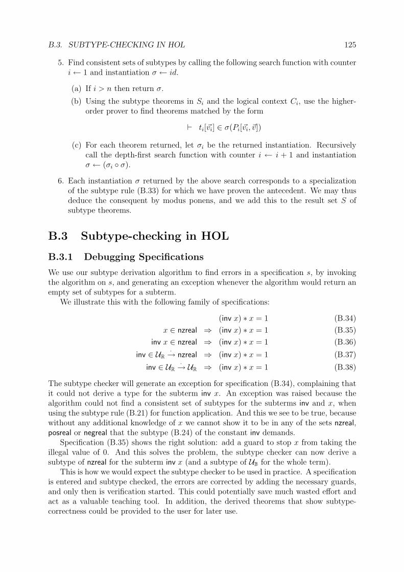
B.3. SUBTYPE-CHECKING IN HOL 125
5. Find consistent sets of subtypes by calling the following search function with counteri← 1 and instantiation σ ← id.
(a) If i > n then return σ.
(b) Using the subtype theorems in Si and the logical context Ci, use the higher-order prover to find theorems matched by the form
` ti[~vi] ∈ σ(Pi[~vi, ~v])
(c) For each theorem returned, let σi be the returned instantiation. Recursivelycall the depth-first search function with counter i ← i + 1 and instantiationσ ← (σi σ).
6. Each instantiation σ returned by the above search corresponds to a specializationof the subtype rule (B.33) for which we have proven the antecedent. We may thusdeduce the consequent by modus ponens, and we add this to the result set S ofsubtype theorems.
B.3 Subtype-checking in HOL
B.3.1 Debugging Specifications
We use our subtype derivation algorithm to find errors in a specification s, by invokingthe algorithm on s, and generating an exception whenever the algorithm would return anempty set of subtypes for a subterm.
We illustrate this with the following family of specifications:
(inv x) ∗ x = 1 (B.34)
x ∈ nzreal ⇒ (inv x) ∗ x = 1 (B.35)
inv x ∈ nzreal ⇒ (inv x) ∗ x = 1 (B.36)
inv ∈ UR·→ nzreal ⇒ (inv x) ∗ x = 1 (B.37)
inv ∈ UR·→ UR ⇒ (inv x) ∗ x = 1 (B.38)
The subtype checker will generate an exception for specification (B.34), complaining thatit could not derive a type for the subterm inv x. An exception was raised because thealgorithm could not find a consistent set of subtypes for the subterms inv and x, whenusing the subtype rule (B.21) for function application. And this we see to be true, becausewithout any additional knowledge of x we cannot show it to be in any of the sets nzreal,posreal or negreal that the subtype (B.24) of the constant inv demands.
Specification (B.35) shows the right solution: add a guard to stop x from taking theillegal value of 0. And this solves the problem, the subtype checker can now derive asubtype of nzreal for the subterm inv x (and a subtype of UB for the whole term).
This is how we would expect the subtype checker to be used in practice. A specificationis entered and subtype checked, the errors are corrected by adding the necessary guards,and only then is verification started. This could potentially save much wasted effort andact as a valuable teaching tool. In addition, the derived theorems that show subtype-correctness could be provided to the user for later use.

126 APPENDIX B. PREDICATE SET PROVER
Specifications (B.36)–(B.38) represent various attempts to subvert the subtype checker.Specification (B.36) is a silly attempt: now the inv x in the antecedent fails to subtypecheck! However, even if the antecedent were added unchecked to the logical context, theconsequent would still not subtype check: an extra subtype for inv x does not help at all inthe search to find consistent subtypes for inv and x using the rule for function application.Specification (B.37) steps up a level in the arms race by assuming a subtype for inv, andnow this term does subtype check since the higher-order prover just needs to show thatx ∈ UR: a triviality. However, we may take consolation in the fact that this antecedent isunprovable. Finally Specification (B.38) is the most worrying attack: the term subtypechecks, and we can use theorem (B.13) to prove the condition.
B.3.2 Logical Limits
In the previous section we showed by example how the subtype checker that we implementmay be duped into passing a term that contains a violation of subtype constraints. Unfor-tunately, this is not just an inadequacy of the subtype checker, but rather an inescapableconsequence of reasoning with predicate sets in the HOL logic. Since HOL is a logic oftotal functions, given any function f : α→ β we can prove the theorem
` f ∈ Uα·→ Uβ (B.39)
since this just expands to` ∀x ∈ Uα. f(x) ∈ Uβ
which is true by the definition of the universal set Uβ.In particular, theorem (B.39) is true for all function constants f that we would like to
have a restricted domain (such as inv). But the subtype Uα → Uβ allows f to be applied toany element of type α. This means that enforceable predicate subtyping using predicatesets cannot exist as a layer on top of the existing HOL kernel.
Example: Even if the user is not trying to subvert the system, it might happen acciden-tally. If we are subtype checking the specification
P ⇒ Q (inv 0)
then when we subtype check the consequent Q (inv 0) we add the antecedent P to thelogical context, and it might transpire that P somehow causes the higher-order prover todeduce inv ∈ UR
·→ UR,18 which then allows Q (inv 0) to be successfully subtype checked.2
To summarize the situation, if a specification fails to subtype-check19 then there’sdefinitely a problem with it, if subtype-checking succeeds then there could be a hiddenproblem with it. It’s like testing: subtype-checking in this context can only show thepresence of errors.
PVS is also a logic of total functions, but the ability to make a first-class type of non-zero reals means that if inv is declared to have type R 6=0 → R 6=0 then the type-system can
18After all, it is a theorem!19with sufficiently generous search bounds

B.4. PREDICATE SET PROVER AND APPLICATIONS 127
stop the function from being ‘lifted’ to a larger type. Essentially the PVS logic implementsa logic of partial functions, but by insisting that a type is available for every function’sdomain can avoid awkward questions of definedness.
B.4 Predicate Set Prover and Applications
B.4.1 Predicate Set Prover
An obvious application for the subtype derivation algorithm is to prove set membershipgoals. Supposing the current goal is t ∈ P , we can derive a set S of subtype theorems fort, and then invoke the higher-order prover once again with the top-level context and theset S to tackle the goal directly. We package up this proof procedure into a HOL tacticcalled the predicate set prover.
Example: To illustrate the two steps of the predicate set prover, consider the goal3 ∈ nzreal.20 Subtypes are derived for the term 3 (of type R), and the following set ofsubtype theorems are returned:
` 3 ∈ K posreal 3, ` 3 ∈ K nnegreal 3
(where K = λx. λ y. x). Next these two theorems are passed to the higher-order proveralong with the top-level logical context containing type-judgements, and it quickly provesthe goal ` 3 ∈ nzreal. 2
We can prove some interesting goals with the predicate set prover:
` map inv (cons (−1) (map sqrt [3, 1])) ∈ list nzreal
` (λx ∈ negreal. funpow inv n x) ∈ negreal·→ negreal
One optimization that is effective with this tactic is to maintain a cache of the subtypesthat have already been derived for HOL constants.21 For example, the innocuous-lookingterm ‘3’ used in the above example is actually composed of 4 nested function applications!Re-deriving subtypes for constants is unnecessary and inefficient.
Another optimization arises naturally from certain subtype rules, such as the conjunc-tion rule (B.20), repeated here:
∀ a, b. (b⇒ a ∈ UB) ∧ (a⇒ b ∈ UB)⇒ (a ∧ b) ∈ UB
The set UB is the universe set UB of booleans, so we can immediately prove ` b⇒ a ∈ UBand ` a ⇒ b ∈ UB without recursing into the structure of the subterms a and b. Notethat if we were deriving subtypes in order to check the term for subtype correctness thenwe would be obliged to carry out this recursion step to check a and b, but if our goal isproving set membership then we can safely skip this.
20This is not quite as trivial as it looks, since the real number ‘3’ in HOL is really the complex termreal of num (numeral (bit1 (bit1 0))).
21Here ‘constant’ means any term having no free variables.

128 APPENDIX B. PREDICATE SET PROVER
The predicate set prover allows us to gain much of the proving benefit that PVS pred-icate subtyping provides,22 and in some ways it does even better: the subtype derivationalgorithm is not restricted to calculating with principal subtypes, but rather with anysubtype that the term can be shown to satisfy using the derivation rules.
B.4.2 Proving Conditions During Rewriting
We can use the predicate set prover as a condition prover in a contextual rewriter, andthere are several reasons why it is useful to integrate these tools:
• There is a trend to incorporate tools into contextual rewriters because of the au-tomatic subterm traversal and context accumulation. The logical context built upby the contextual rewriter is easily transferred to the predicate set prover, and thesubterm traversal allows us to attempt a proof of all occurrences of t ∈ P in thegoal term.23
• Many rewrites have side conditions that can be expressed very naturally using re-stricted quantifiers, and these generate goals for the predicate set prover when therewrite is applied.
• Subtype judgements, rules and constants can be stored with the simplification setof a theory, thus reducing the administration burden of theory-specific rules.
Here are some miscellaneous rewrite rules that make use of subtype conditions:
` ∀x ∈ nzreal. x/x = 1 (B.40)
` ∀n. ∀m ∈ lenum n. m+ (n−m) = n (B.41)
` ∀n ∈ nznum. n mod n = 0 (B.42)
` ∀ s ∈ finite. ∀ f ∈ injection s. |image f s| = |s| (B.43)
` ∀G ∈ group. ∀ g ∈ set G. idG ∗G g = g (B.44)
` ∀G ∈ group. ∀ g, h ∈ set G. (g ∗G h = h) = (g = idG) (B.45)
Using rule (B.40), a term like 5/5 = 3/3 is straightforwardly rewritten to >. The lasttwo examples come from a body of computational number theory that we formalized toverify the Miller-Rabin probabilistic primality test (Chapter 5).
An effective optimization for this tool is to make adding assumptions into the subtypelogical context a lazy operation. This delays their conversion to combinatory form andCNF normalization until the predicate set prover is invoked on a goal, which might nothappen at all.
In theory, the architecture laid out in this chapter can establish much more exoticproperties than these, but the predicate subtype prover was found to be most useful
22Although almost certainly the performance using our model is worse than implementing predicatesubtyping as part of the logic: keeping subtypes with the terms so they never have to be re-derivedmust provide a boost. We also experimented with this kind of architecture, but eventually dropped it tosimplify the design and increase interoperability with existing tools.
23When subtype derivation is applied to a subterm it accumulates context in much the same wayas a contextual rewriter. However, despite this similarity, the two tools are orthogonal and are bestimplemented separately: we tried both approaches.

B.5. CONCLUDING REMARKS 129
and robust on these relatively simple properties that come up again and again duringconditional rewriting. These properties naturally propagate upwards through a term,being preserved by most of the basic operations, and in such situations the predicate setprover can be relied upon to show the desired condition (albeit sometimes rather slowly).This tool lent itself to more efficient development of the required theories, particularlythe group theory where almost every theorem has one or more group membership side-conditions. Our evaluation is that it is a useful tool for reasoning about term propertiesthat naturally propagate up terms.
B.5 Concluding Remarks
We have demonstrated that predicate subtyping can be simulated in HOL using predicatesets, and presented a new automatic proof procedure that takes advantage of this newstyle of reasoning. This proved to be an effective proof tool on a case study of formalizedcomputational number theory.
A comparison of HOL and PVS was made by Gordon (1996) from the perspectives oflogic, automatic proof and usability. The model of predicate subtyping using predicatesets builds upon HOL88 restricted quantifier library of Wong (1993), and the exact detailsof the predicate subtyping in our model attempts to follow the PVS architecture. For thefull details of the semantics and implementation of subtyping in PVS, refer to Owre andShankar (1997).
Previous work in this area has been done by Jones (1997), who built a tool in HOL tospecify the subtype of constants and subtype check terms with respect to the subtypes.Given a term t, the tool sets up HOL goals that, if proved, would correspond to theterm being subtype-correct. The user is then free to use these extra theorems duringverification. Our model extends Jones’ by the introduction of subtype rules for generatingtype-correctness conditions, the higher-order prover to automatically prove conditions,and the integration of the tool into a rewriter to aid interactive proof.
ACL2 uses guards (Kaufmann and Moore, 1997) to stop functions from being appliedoutside their domain; these generate proof obligations when new functions are definedin terms of guarded functions. When the proof obligations have been satisfied the newfunction is given a ‘gold’ status, and can be safely executed without causing run-time typeerrors. This is very similar to the way PVS type-checks terms before admitting them intothe system.
A system of guard formulas in Z/EVES has also been implemented by Saaltink (1997);similarly to our work these guards are used to aid formal Z proofs and find errors inZ specifications. The Z logic allows terms to be ‘undefined’, but the system of guardformulas imposed will flag the situations that can result in undefinedness, allowing classicalreasoning on the partial logic. Since Z is based on set theory, this use of guards does notsuffer from the logical limitations we outlined in Section B.3.2, and can provide strongguarantees about a checked specification. However, whereas our subtype rules propagateall available logical information around the term, Saaltink chooses a “left-to-right systemof interpretation” that is not complete, but works well in most practical situations andsimplifies guard conditions.
There has also been a huge amount of work on subtyping and polymorphism in variousλ-calculi, used to model object-oriented programming languages. Some concepts from this

130 APPENDIX B. PREDICATE SET PROVER
field are related to our work, in particular the notion of intersection types corresponds tofinding multiple subtypes of a term. The thesis of Compagnoni (1995) provides a goodintroduction to this area.
Since we now have a preliminary evaluation of the predicate subtype prover, we mustdecide the direction in which to advance it. On the one hand it may be possible to widenits effective scope by including rules for building up more complicated predicate sets, oron the other hand it may be most useful to speed up the performance and make it morerobust on the scope we have identified here. The path we take may depend on how farwe can push the underlying higher-order prover.
Another interesting extension to this research would be to use subtype checking toperform subtype inference of new constants. This would be extremely useful: currentlyfor each constant which we would like to add to the constant subtype dictionary, we mustprove a result of the form of theorems (B.24)–(B.30). One way to approach this taskwould be to initially set the type of the new constant c to be c ∈ P where P is a variable;during subtype checking collect constraints on P ; and finally at the top-level try to solvethese constraints: the solutions being subtypes for c.
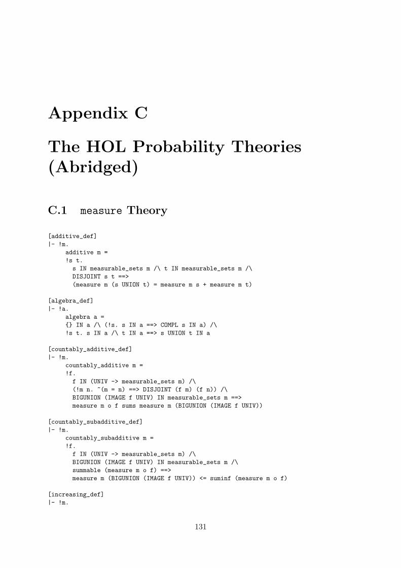
Appendix C
The HOL Probability Theories(Abridged)
C.1 measure Theory
[additive_def]|- !m.
additive m =!s t.s IN measurable_sets m /\ t IN measurable_sets m /\DISJOINT s t ==>(measure m (s UNION t) = measure m s + measure m t)
[algebra_def]|- !a.
algebra a = IN a /\ (!s. s IN a ==> COMPL s IN a) /\!s t. s IN a /\ t IN a ==> s UNION t IN a
[countably_additive_def]|- !m.
countably_additive m =!f.f IN (UNIV -> measurable_sets m) /\(!m n. ~(m = n) ==> DISJOINT (f m) (f n)) /\BIGUNION (IMAGE f UNIV) IN measurable_sets m ==>measure m o f sums measure m (BIGUNION (IMAGE f UNIV))
[countably_subadditive_def]|- !m.
countably_subadditive m =!f.f IN (UNIV -> measurable_sets m) /\BIGUNION (IMAGE f UNIV) IN measurable_sets m /\summable (measure m o f) ==>measure m (BIGUNION (IMAGE f UNIV)) <= suminf (measure m o f)
[increasing_def]|- !m.
131

132 APPENDIX C. THE HOL PROBABILITY THEORIES
increasing m =!s t.s IN measurable_sets m /\ t IN measurable_sets m /\s SUBSET t ==>measure m s <= measure m t
[inf_measure_def]|- !m s.
inf_measure m s =infr|?f.
f IN (UNIV -> measurable_sets m) /\(!m n. ~(m = n) ==> DISJOINT (f m) (f n)) /\s SUBSET BIGUNION (IMAGE f UNIV) /\ measure m o f sums r
[lambda_system_def]|- !g0 lam.
lambda_system g0 lam =l|l IN g0 /\!g. g IN g0 ==> (lam (l INTER g) + lam (COMPL l INTER g) = lam g)
[measurable_def]|- !a b. measurable a b = f | !s. s IN b ==> PREIMAGE f s IN a
[measurable_sets_def]|- !a mu. measurable_sets (a,mu) = a
[measure_def]!a mu. measure (a,mu) = mu
[measure_preserving_def]|- !m1 m2.
measure_preserving m1 m2 =f|f IN measurable (measurable_sets m1) (measurable_sets m2) /\!s.
s IN measurable_sets m2 ==>(measure m1 (PREIMAGE f s) = measure m2 s)
[measure_space_def]|- !m.
measure_space m =sigma_algebra (measurable_sets m) /\ positive m /\countably_additive m
[outer_measure_space_def]|- !m.
outer_measure_space m =positive m /\ increasing m /\ countably_subadditive m
[positive_def]

C.1. MEASURE THEORY 133
|- !m.positive m =(measure m = 0) /\!s. s IN measurable_sets m ==> 0 <= measure m s
[sigma_algebra_def]|- !a.
sigma_algebra a =algebra a /\ !c. countable c /\ c SUBSET a ==> BIGUNION c IN a
[sigma_def]|- !b. sigma b = BIGINTER a | b SUBSET a /\ sigma_algebra a
[subadditive_def]|- !m.
subadditive m =!s t.s IN measurable_sets m /\ t IN measurable_sets m ==>measure m (s UNION t) <= measure m s + measure m t
[ADDITIVE_INCREASING]|- !m.
algebra (measurable_sets m) /\ positive m /\ additive m ==>increasing m
[ALGEBRA_COMPL]|- !a s. algebra a /\ s IN a ==> COMPL s IN a
[ALGEBRA_DIFF]|- !a s t. algebra a /\ s IN a /\ t IN a ==> s DIFF t IN a
[ALGEBRA_EMPTY]|- !a. algebra a ==> IN a
[ALGEBRA_FINITE_UNION]|- !a c. algebra a /\ FINITE c /\ c SUBSET a ==> BIGUNION c IN a
[ALGEBRA_INTER]|- !a s t. algebra a /\ s IN a /\ t IN a ==> s INTER t IN a
[ALGEBRA_SUBSET_LAMBDA_SYSTEM]|- !m.
algebra (measurable_sets m) /\ positive m /\ increasing m /\additive m ==>measurable_sets m SUBSET lambda_system UNIV (inf_measure m)
[ALGEBRA_UNION]|- !a s t. algebra a /\ s IN a /\ t IN a ==> s UNION t IN a
[ALGEBRA_UNIV]|- !a. algebra a ==> UNIV IN a
[CARATHEODORY]|- !m0.
algebra (measurable_sets m0) /\ positive m0 /\countably_additive m0 ==>

134 APPENDIX C. THE HOL PROBABILITY THEORIES
?m.(!s. s IN measurable_sets m0 ==> (measure m s = measure m0 s)) /\(measurable_sets m = sigma (measurable_sets m0)) /\measure_space m
[CARATHEODORY_LEMMA]|- !gsig lam.
sigma_algebra gsig /\ outer_measure_space (gsig,lam) ==>measure_space (lambda_system gsig lam,lam)
[COUNTABLY_ADDITIVE_ADDITIVE]|- !m.
algebra (measurable_sets m) /\ positive m /\countably_additive m ==>additive m
[COUNTABLY_SUBADDITIVE_SUBADDITIVE]|- !m.
algebra (measurable_sets m) /\ positive m /\countably_subadditive m ==>subadditive m
[INCREASING_ADDITIVE_SUMMABLE]|- !m f.
algebra (measurable_sets m) /\ positive m /\ increasing m /\additive m /\ f IN (UNIV -> measurable_sets m) /\(!m n. ~(m = n) ==> DISJOINT (f m) (f n)) ==>summable (measure m o f)
[INF_MEASURE_AGREES]|- !m s.
algebra (measurable_sets m) /\ positive m /\countably_additive m /\ s IN measurable_sets m ==>(inf_measure m s = measure m s)
[INF_MEASURE_OUTER]|- !m.
algebra (measurable_sets m) /\ positive m /\ increasing m ==>outer_measure_space (UNIV,inf_measure m)
[IN_SIGMA]|- !a x. x IN a ==> x IN sigma a
[LAMBDA_SYSTEM_ADDITIVE]|- !g0 lam l1 l2.
algebra g0 /\ positive (g0,lam) ==>additive (lambda_system g0 lam,lam)
[LAMBDA_SYSTEM_ALGEBRA]|- !g0 lam.
algebra g0 /\ positive (g0,lam) ==> algebra (lambda_system g0 lam)
[LAMBDA_SYSTEM_CARATHEODORY]|- !gsig lam.
sigma_algebra gsig /\ outer_measure_space (gsig,lam) ==>!f.

C.1. MEASURE THEORY 135
f IN (UNIV -> lambda_system gsig lam) /\(!m n. ~(m = n) ==> DISJOINT (f m) (f n)) ==>BIGUNION (IMAGE f UNIV) IN lambda_system gsig lam /\lam o f sums lam (BIGUNION (IMAGE f UNIV))
[LAMBDA_SYSTEM_INCREASING]|- !g0 lam.
increasing (g0,lam) ==> increasing (lambda_system g0 lam,lam)
[LAMBDA_SYSTEM_POSITIVE]|- !g0 lam. positive (g0,lam) ==> positive (lambda_system g0 lam,lam)
[MEASURABLE_COMP]|- !f g a b c.
f IN measurable a b /\ g IN measurable b c ==>g o f IN measurable a c
[MEASURABLE_I]|- !a. I IN measurable a a
[MEASURABLE_LIFT]|- !f a b.
sigma_algebra a /\ f IN measurable a b ==>f IN measurable a (sigma b)
[MEASURABLE_PROD_SIGMA]|- !a a1 a2 f.
sigma_algebra a /\ FST o f IN measurable a a1 /\SND o f IN measurable a a2 ==>f IN measurable a (sigma (prod_sets a1 a2))
[MEASURABLE_UP_LIFT]|- !a b c f. f IN measurable a c /\ a SUBSET b ==> f IN measurable b c
[MEASURE_PRESERVING_LIFT]|- !m1 m2 a f.
measure_space m1 /\ measure_space m2 /\ algebra a /\(measurable_sets m2 = sigma a) /\f IN measure_preserving m1 (a,measure m2) ==>f IN measure_preserving m1 m2
[MEASURE_PRESERVING_UP_LIFT]|- !m1 m2 f.
f IN measure_preserving (a,measure m1) m2 /\a SUBSET measurable_sets m1 ==>f IN measure_preserving m1 m2
[MEASURE_SPACE_REDUCE]|- !m. (measurable_sets m,measure m) = m
[MONOTONE_CONVERGENCE]|- !m s f.
measure_space m /\ f IN (UNIV -> measurable_sets m) /\(!n. f n SUBSET f (SUC n)) /\ (s = BIGUNION (IMAGE f UNIV)) ==>measure m o f --> measure m s

136 APPENDIX C. THE HOL PROBABILITY THEORIES
[SIGMA_ALGEBRA]|- !p.
sigma_algebra p = IN p /\ (!s. s IN p ==> COMPL s IN p) /\!c. countable c /\ c SUBSET p ==> BIGUNION c IN p
[SIGMA_ALGEBRA_SIGMA]|- !b. sigma_algebra (sigma b)
[SIGMA_PROPERTY]|- !p a.
IN p /\ a SUBSET p /\(!s. s IN p INTER sigma a ==> COMPL s IN p) /\(!c.
countable c /\ c SUBSET p INTER sigma a ==> BIGUNION c IN p) ==>sigma a SUBSET p
[SIGMA_PROPERTY_DISJOINT]|- !p a.
algebra a /\ a SUBSET p /\(!s. s IN p INTER sigma a ==> COMPL s IN p) /\(!f.
f IN (UNIV -> p INTER sigma a) /\ (f 0 = ) /\(!n. f n SUBSET f (SUC n)) ==>BIGUNION (IMAGE f UNIV) IN p) /\
(!f.f IN (UNIV -> p INTER sigma a) /\(!m n. ~(m = n) ==> DISJOINT (f m) (f n)) ==>BIGUNION (IMAGE f UNIV) IN p) ==>
sigma a SUBSET p
[UNIV_SIGMA_ALGEBRA]|- sigma_algebra UNIV
C.2 probability Theory
[events_def]|- events = measurable_sets
[indep_def]|- !p a b.
indep p a b =a IN events p /\ b IN events p /\(prob p (a INTER b) = prob p a * prob p b)
[indep_families_def]|- !p q r. indep_families p q r = !s t. s IN q /\ t IN r ==> indep p s t
[indep_function_def]|- !p.
indep_function p =f |

C.2. PROBABILITY THEORY 137
indep_families p (IMAGE (PREIMAGE (FST o f)) UNIV)(IMAGE (PREIMAGE (SND o f)) (events p))
[possibly_def]|- !p e. possibly p e = e IN events p /\ ~(prob p e = 0)
[prob_def]|- prob = measure
[prob_preserving_def]|- prob_preserving = measure_preserving
[prob_space_def]|- !p. prob_space p = measure_space p /\ (measure p UNIV = 1)
[probably_def]|- !p e. probably p e = e IN events p /\ (prob p e = 1)
[EVENTS]|- !a b. events (a,b) = a
[EVENTS_SIGMA_ALGEBRA]|- !p. prob_space p ==> sigma_algebra (events p)
[INDEP_EMPTY]|- !p s. prob_space p /\ s IN events p ==> indep p s
[INDEP_REFL]|- !p a.
prob_space p /\ a IN events p ==>(indep p a a = (prob p a = 0) \/ (prob p a = 1))
[INDEP_SYM]|- !p a b. prob_space p /\ indep p a b ==> indep p b a
[INDEP_UNIV]|- !p s. prob_space p /\ s IN events p ==> indep p UNIV s
[PROB]|- !a b. prob (a,b) = b
[PROB_ADDITIVE]|- !p s t u.
prob_space p /\ s IN events p /\ t IN events p /\ DISJOINT s t /\(u = s UNION t) ==>(prob p u = prob p s + prob p t)
[PROB_COMPL]|- !p s.
prob_space p /\ s IN events p ==> (prob p (COMPL s) = 1 - prob p s)
[PROB_COUNTABLY_ADDITIVE]|- !p s f.
prob_space p /\ f IN (UNIV -> events p) /\(!m n. ~(m = n) ==> DISJOINT (f m) (f n)) /\(s = BIGUNION (IMAGE f UNIV)) ==>

138 APPENDIX C. THE HOL PROBABILITY THEORIES
prob p o f sums prob p s
[PROB_EMPTY]|- !p. prob_space p ==> (prob p = 0)
[PROB_FINITELY_ADDITIVE]|- !p s f n.
prob_space p /\ f IN (count n -> events p) /\(!a b. a < n /\ b < n /\ ~(a = b) ==> DISJOINT (f a) (f b)) /\(s = BIGUNION (IMAGE f (count n))) ==>(sum (0,n) (prob p o f) = prob p s)
[PROB_INCREASING]|- !p s t.
prob_space p /\ s IN events p /\ t IN events p /\ s SUBSET t ==>prob p s <= prob p t
[PROB_INCREASING_UNION]|- !p s f.
prob_space p /\ f IN (UNIV -> events p) /\(!n. f n SUBSET f (SUC n)) /\ (s = BIGUNION (IMAGE f UNIV)) ==>prob p o f --> prob p s
[PROB_LE_1]|- !p s. prob_space p /\ s IN events p ==> prob p s <= 1
[PROB_ONE_INTER]|- !p s t.
prob_space p /\ s IN events p /\ t IN events p /\(prob p t = 1) ==>(prob p (s INTER t) = prob p s)
[PROB_POSITIVE]|- !p s. prob_space p /\ s IN events p ==> 0 <= prob p s
[PROB_PRESERVING]|- !p1 p2.
prob_preserving p1 p2 =f |f IN measurable (events p1) (events p2) /\!s. s IN events p2 ==> (prob p1 (PREIMAGE f s) = prob p2 s)
[PROB_PRESERVING_LIFT]|- !p1 p2 a f.
prob_space p1 /\ prob_space p2 /\ algebra a /\(events p2 = sigma a) /\ f IN prob_preserving p1 (a,prob p2) ==>f IN prob_preserving p1 p2
[PROB_PRESERVING_UP_LIFT]|- !p1 p2 f.
f IN prob_preserving (a,prob p1) p2 /\ a SUBSET events p1 ==>f IN prob_preserving p1 p2
[PROB_SPACE]|- !p.
prob_space p =
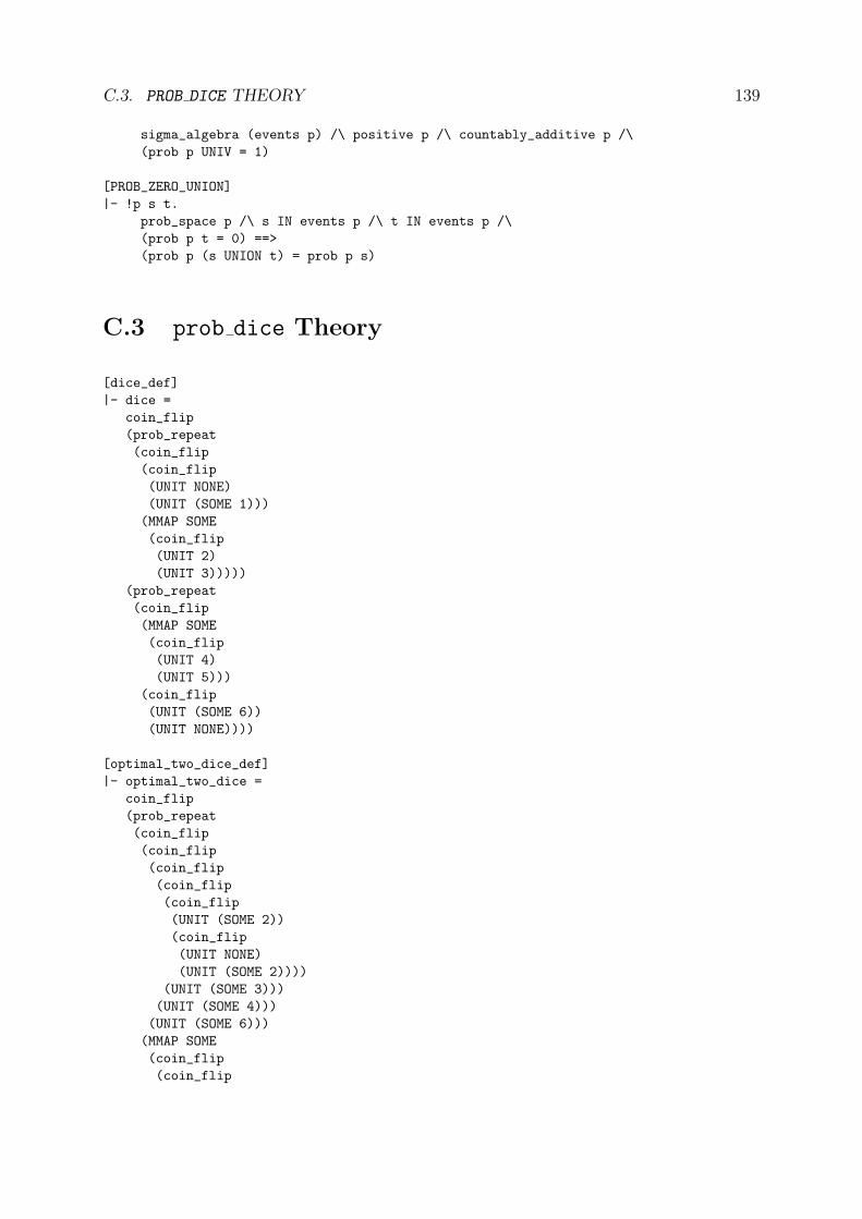
C.3. PROB DICE THEORY 139
sigma_algebra (events p) /\ positive p /\ countably_additive p /\(prob p UNIV = 1)
[PROB_ZERO_UNION]|- !p s t.
prob_space p /\ s IN events p /\ t IN events p /\(prob p t = 0) ==>(prob p (s UNION t) = prob p s)
C.3 prob dice Theory
[dice_def]|- dice =
coin_flip(prob_repeat(coin_flip(coin_flip(UNIT NONE)(UNIT (SOME 1)))(MMAP SOME(coin_flip(UNIT 2)(UNIT 3)))))
(prob_repeat(coin_flip(MMAP SOME(coin_flip(UNIT 4)(UNIT 5)))
(coin_flip(UNIT (SOME 6))(UNIT NONE))))
[optimal_two_dice_def]|- optimal_two_dice =
coin_flip(prob_repeat(coin_flip(coin_flip(coin_flip(coin_flip(coin_flip(UNIT (SOME 2))(coin_flip(UNIT NONE)(UNIT (SOME 2))))
(UNIT (SOME 3)))(UNIT (SOME 4)))(UNIT (SOME 6)))(MMAP SOME(coin_flip(coin_flip

140 APPENDIX C. THE HOL PROBABILITY THEORIES
(coin_flip(coin_flip(UNIT 3)(coin_flip(coin_flip(UNIT 2)(UNIT 4))(UNIT 3)))
(UNIT 5))(UNIT 5))(UNIT 7)))))
(prob_repeat(coin_flip(MMAP SOME(coin_flip(coin_flip(coin_flip(coin_flip(UNIT 4)(coin_flip(UNIT 6)(coin_flip(UNIT 6)(UNIT 8))))
(UNIT 7))(UNIT 9))(UNIT 8)))
(coin_flip(MMAP SOME(coin_flip(coin_flip(coin_flip(UNIT 5)(UNIT 9))
(UNIT 9))(UNIT 10)))
(coin_flip(MMAP SOME(coin_flip(coin_flip(coin_flip(UNIT 7)(UNIT 8))(UNIT 10))
(UNIT 11)))(coin_flip(MMAP SOME(coin_flip(coin_flip(coin_flip(UNIT 10)(UNIT 12))(UNIT 11))(UNIT 11)))
(coin_flip(coin_flip

C.3. PROB DICE THEORY 141
(UNIT (SOME 12))(UNIT NONE))
(UNIT (SOME 12))))))))
[two_dice_def]|- two_dice = BIND dice (\a. BIND dice (\b. UNIT (a + b)))
[INDEP_FN_DICE]|- dice IN indep_fn
[INDEP_FN_OPTIMAL_TWO_DICE]|- optimal_two_dice IN indep_fn
[INDEP_FN_TWO_DICE]|- two_dice IN indep_fn
[OPTIMAL_TWO_DICE_CORRECT]|- !n.
prob bern s | FST (optimal_two_dice s) = n =prob bern s | FST (two_dice s) = n
[PROB_BERN_DICE]|- !n.
prob bern s | FST (dice s) = n =(if 1 <= n /\ n <= 6 then 1 / 6 else 0)
[PROB_BERN_TWO_DICE]|- !n.
prob bern s | FST (two_dice s) = n =(if (n = 2) \/ (n = 12) then 1 / 36else if (n = 3) \/ (n = 11) then 2 / 36else if (n = 4) \/ (n = 10) then 3 / 36else if (n = 5) \/ (n = 9) then 4 / 36else if (n = 6) \/ (n = 8) then 5 / 36else if n = 7 then 6 / 36else 0)

142 APPENDIX C. THE HOL PROBABILITY THEORIES

Appendix D
Miller-Rabin Primality TestExtracted to Standard ML
D.1 HOL miller rabin ml Theory
[BIND_ML]|- !f g. BIND f g = UNCURRY g o f
[EVEN_ML]|- !n. EVEN n = (n MOD 2 = 0)
[FACTOR_TWOS_ML]|- factor_twos n =
(if 0 < n /\ EVEN n then(let (r,s) = factor_twos (n DIV 2) in (SUC r,s))
else(0,n))
[LOG2_ML]|- !n. log2 n = (if n = 0 then 0 else SUC (log2 (n DIV 2)))
[MANY_ML]|- !f n.
MANY f n =(if n = 0 then
UNIT TelseBIND f (\x. (if x then MANY f (n - 1) else UNIT F)))
[MILLER_RABIN_1_ML]|- !n.
miller_rabin_1 n =(if n = 2 then
UNIT Telse(if (n = 1) \/ EVEN n then
UNIT FelseBIND (prob_uniform_cut (2 * log2 (n - 1)) (n - 2))
143

144 APPENDIX D. MILLER-RABIN PRIMALITY TEST IN ML
(\a. ~witness n (a + 2))))
[MILLER_RABIN_ML]|- !n t. miller_rabin n t = MANY (miller_rabin_1 n) t
[MODEXP_ML]|- modexp n a b =
(if b = 0 then1
else(let r = modexp n a (b DIV 2) in
let r2 = (r * r) MOD n in(if EVEN b then r2 else (r2 * a) MOD n)))
[ODD_ML]|- ODD = $~ o EVEN
[PROB_UNIFORM_CUT_ML]|- !t n.
prob_uniform_cut t n =(if n = 0 then
prob_uniform_cut t nelse(if t = 0 then
UNIT 0elseBIND (prob_unif (n - 1))(\m. if m < n then UNIT m else prob_uniform_cut (t - 1) n)))
[PROB_UNIF_ML]|- !n.
prob_unif n =(if n = 0 then
UNIT 0elseBIND (prob_unif (n DIV 2))(\m. BIND sdest (\b. if b then 2 * m + 1 else 2 * m)))
[UNCURRY_ML]|- !f x y. UNCURRY f (x,y) = f x y
[UNIT_ML]|- !x. UNIT x = (\s. (x,s))
[WITNESS_ML]|- !n a.
witness n a =(let (r,s) = factor_twos (n - 1) in
witness_tail n (modexp n a s) r)
[WITNESS_TAIL_ML]|- !n a r.
witness_tail n a r =(if r = 0 then
~(a = 1)else

D.2. ML SUPPORT MODULES 145
(let a2 = (a * a) MOD n in(if a2 = 1 then
~(a = 1) /\ ~(a = n - 1)elsewitness_tail n a2 (r - 1))))
D.2 ML Support Modules
D.2.1 HolStream Signature
signature HolStream =sigtype ’a stream = ’a Stream.stream
val shd : ’a stream -> ’aval stl : ’a stream -> ’a streamval sdest : ’a stream -> ’a * ’a stream
end
This module provides a HOL wrapper to a more comprehensive Stream module.
D.2.2 RandomBits Signature
signature RandomBits =sigval random : unit -> bool Stream.streamval urandom : unit -> bool Stream.stream
end
In this module, the values random and urandom provide an interface to the Linux devices/dev/random and /dev/urandom.
D.2.3 HolNum Signature
signature HolNum =sigtype num
val num_to_bits : num -> bool listval bits_to_num : bool list -> num
val Num : string -> numval num_to_string : num -> stringval pp_num : ppstream -> num -> unit
val ZERO : numval ONE : num

146 APPENDIX D. MILLER-RABIN PRIMALITY TEST IN ML
val TWO : num
val SUC : num -> numval ++ : num * num -> numval -- : num * num -> numval ** : num * num -> numval DIV : num * num -> numval MOD : num * num -> num
val == : num * num -> boolval <<= : num * num -> boolval >>= : num * num -> boolval << : num * num -> boolval >> : num * num -> bool
end
This module provides support for a type num of arbitrarily large natural numbers.
D.3 ML Miller-Rabin
D.3.1 HolMiller.sml Structure
structure HolMiller :> HolMiller =struct
open HolNum HolStream;
infix 7 ** MOD DIV;infix 6 ++ --;infix 4 == <<= << >>= >>;
(* pair *)
fun UNCURRY f (x, y) = f x y;
(* state_transformer *)
fun UNIT x = fn s => (x, s);
fun BIND f g = UNCURRY g o f;
(* num *)
fun EVEN n = (n MOD TWO == ZERO);
val ODD = not o EVEN;
(* prob *)
fun MANY f n =if n == ZERO then UNIT trueelse BIND f (fn x => if x then MANY f (n -- ONE) else UNIT false);
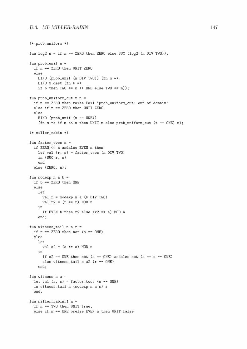
D.3. ML MILLER-RABIN 147
(* prob_uniform *)
fun log2 n = if n == ZERO then ZERO else SUC (log2 (n DIV TWO));
fun prob_unif n =if n == ZERO then UNIT ZEROelseBIND (prob_unif (n DIV TWO)) (fn m =>BIND S.dest (fn b =>if b then TWO ** m ++ ONE else TWO ** m));
fun prob_uniform_cut t n =if n == ZERO then raise Fail "prob_uniform_cut: out of domain"else if t == ZERO then UNIT ZEROelseBIND (prob_unif (n -- ONE))(fn m => if m << n then UNIT m else prob_uniform_cut (t -- ONE) n);
(* miller_rabin *)
fun factor_twos n =if ZERO << n andalso EVEN n thenlet val (r, s) = factor_twos (n DIV TWO)in (SUC r, s)end
else (ZERO, n);
fun modexp n a b =if b == ZERO then ONEelseletval r = modexp n a (b DIV TWO)val r2 = (r ** r) MOD n
inif EVEN b then r2 else (r2 ** a) MOD n
end;
fun witness_tail n a r =if r == ZERO then not (a == ONE)elseletval a2 = (a ** a) MOD n
inif a2 == ONE then not (a == ONE) andalso not (a == n -- ONE)else witness_tail n a2 (r -- ONE)
end;
fun witness n a =let val (r, s) = factor_twos (n -- ONE)in witness_tail n (modexp n a s) rend;
fun miller_rabin_1 n =if n == TWO then UNIT true,else if n == ONE orelse EVEN n then UNIT false
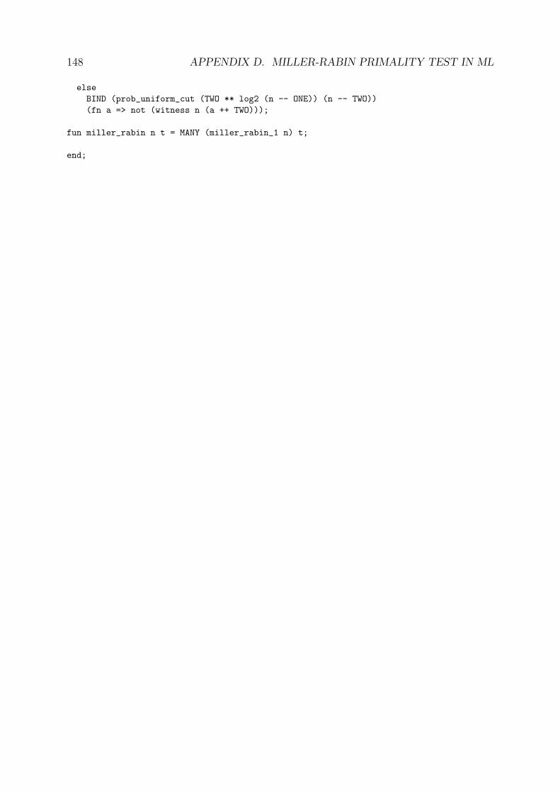
148 APPENDIX D. MILLER-RABIN PRIMALITY TEST IN ML
elseBIND (prob_uniform_cut (TWO ** log2 (n -- ONE)) (n -- TWO))(fn a => not (witness n (a ++ TWO)));
fun miller_rabin n t = MANY (miller_rabin_1 n) t;
end;

Bibliography
Mark Aagaard and John Harrison, editors. Theorem Proving in Higher Order Logics, 13thInternational Conference: TPHOLs 2000, volume 1869 of Lecture Notes in ComputerScience, Portland, OR, USA, August 2000. Springer.
Martin Abadi and Joseph Y. Halpern. Decidability and expressiveness for first-order logicsof probability. Information and Computation, 1994.
Anonymous. The QED manifesto. In Bundy (1994).
Alan Baker. A Concise Introduction to the Theory of Numbers. Cambridge UniversityPress, 1984.
Paul H. Bardell, W. H. McAnney, and J. Savir. Built In Test for VLSI: PseudorandomTechniques. John Wiley, October 1987. URL http://www.wiley.com/Corporate/
Website/Objects/Products/0,9049,65654,00%.html.
Bruno Barras. Programming and computing in HOL. In Aagaard and Harrison (2000),pages 17–37.
E. R. Berlekamp. Factoring polynomials over large finite fields. Math. Comput., 24, 1970.
Jozef Bia las. The σ-additive measure theory. Journal of Formalized Mathematics, 1990.URL http://mizar.uwb.edu.pl/JFM/Vol2/measure1.html.
Jozef Bia las. Properties of Caratheodor’s measure. Journal of Formalized Mathematics,1992. URL http://mizar.uwb.edu.pl/JFM/Vol4/measure4.html.
P. Billingsley. Probability and Measure. John Wiley & Sons, Inc., New York, 2nd edition,1986.
George Boole. The Mathematical Analysis of Logic, Being an Essay Toward a Calculusof Deductive Reasoning. Macmillan, Cambridge, 1847.
Robert S. Boyer, N. G. de Bruijn, Gerard Huet, and Andrzej Trybulec. A mechanicallyproof-checked encyclopedia of mathematics: Should we build one? can we? In Bundy(1994), pages 237–251.
Robert S. Boyer and J Strother Moore. Proof checking the RSA public key encryptionalgorithm. American Mathematical Monthly, 91(3):181–189, 1984. URL http://www.
cs.utexas.edu/users/boyer/rsa.ps.Z.
149

150 BIBLIOGRAPHY
G. Buffon. Essai d’arithmetique morale. Supplement a l’Histoire Naturelle, 4, 1777.
Alan Bundy, editor. 12th International Conference on Automated Deduction (CADE-12), volume 814 of Lecture Notes in Artificial Intelligence, Nancy, France, June 1994.Springer.
Michael Burrows, Martın Abadi, and Roger Needham. A logic of authentication. ACMTransactions on Computer Systems, 8(1):18–36, February 1990. URL http://www.acm.
org/pubs/articles/journals/tocs/1990-8-1/p18-burrows/p18%-burrows.pdf.
O. Caprotti and M. Oostdijk. Formal and efficient primality proofs by use of computeralgebra oracles. Journal of Symbolic Computation, 32(1–2):55–70, 2001. Special Issueon Computer Algebra and Mechanized Reasoning.
Alonzo Church. A formulation of the simple theory of types. Journal of Symbolic Logic,5:56–68, 1940.
Bob Colwell and Bob Brennan. Intel’s formal verification experience on the Willamettedevelopment. In Aagaard and Harrison (2000), pages 106–107.
Adriana B. Compagnoni. Higher-Order Subtyping with Intersection Types. PhD thesis,Catholic University, Nigmegen, January 1995.
Thomas H. Cormen, Charles Eric Leiserson, and Ronald L. Rivest. Introduction to Algo-rithms. MIT Press/McGraw-Hill, Cambridge, Massachusetts, 1990.
Paul Curzon. The formal verification of the Fairisle ATM switching element: an overview.Technical Report 328, University of Cambridge Computer Laboratory, March 1994.
N. de Bruijn. The mathematical language AUTOMATH, its usage, and some of itsextensions. In Symposium on Automatic Demonstration, pages 29–61. Lecture Notes inMathematics, 125, Springer, 1970.
K. de Leeuw, E. F. Moore, C. E. Shannon, and N. Shapiro. Computability by probabilisticmachines. In C. E. Shannon and J. McCarthy, editors, Automata Studies, pages 183–212. Princeton University Press, Princeton, NJ, 1955.
Morris DeGroot. Probability and Statistics. Addison-Wesley, 2nd edition, 1989.
E. W. Dijkstra. A Discipline of Programming. Prentice Hall, 1976.
Euclid. Elements, 300B.C. URL http://www-groups.dcs.st-andrews.ac.uk/
~history/Mathematicians/Euclid.h%tml.
V. A. Feldman and D. Harel. A probabilistic dynamic logic. Journal of Computer andSystem Sciences, 28(2):193–215, 1984.
George S. Fishman. Monte Carlo: Concepts, Algorithms and Applications. Springer, 1996.
J. D. Fleuriot. A Combination of Geometry Theorem Proving and Nonstandard Analysis,with Application to Newton’s Principia. Distinguished Dissertations. Springer, 2001.
BIBLIOGRAPHY 151
J. T. Gill. Computational complexity of probabilistic Turing machines. SIAM Journal onComputing, 6(4):675–695, December 1977.
K. Godel. Uber formal unentscheidbare Satze der Principia Mathematica und verwandterSysteme. Monatshefte fur Mathematik und Physik, 38:173–198, 1931.
Charles M. Goldie and Richard G. E. Pinch. Communication theory, volume 20 of LMSStudent Texts. Cambridge University Press, 1991.
M. Gordon, R. Milner, and C. Wadsworth. Edinburgh LCF, volume 78 of Lecture Notesin Computer Science. Springer, 1979.
M. J. C. Gordon. HOL: A proof generating system for higher-order logic. In G. M.Birtwistle and P. A. Subrahmanyam, editors, VLSI Specification, Verification and Syn-thesis, pages 73–128. Kluwer Academic Publishers, Boston, 1988.
M. J. C. Gordon. Notes on PVS from a HOL perspective. URL http://www.cl.cam.ac.
uk/~mjcg/PVS.html. Available from the author’s web page, 1996.
M. J. C. Gordon and T. F. Melham. Introduction to HOL (A theorem-proving environmentfor higher order logic). Cambridge University Press, 1993.
Elsa Gunter. Doing algebra in simple type theory. Technical Report MS-CIS-89-38, Logic& Computation 09, Department of Computer and Information Science, University ofPennsylvania, 1989.
Joseph Y. Halpern. An analysis of first-order logics of probability. Artificial Intelligence,1990. URL http://www.cs.cornell.edu/home/halpern/abstract.html#journal25.
R. W. Hansell. Borel measurable mappings for nonseparable metric spaces. Transactionsof the American Mathematical Society, 161:145–169, November 1971. URL http://
uk.jstor.org/cgi-bin/jstor/listjournal/00029947/di970179.
G. H. Hardy. A Mathematician’s Apology, reprinted with a foreword by C. P. Snow.Cambridge University Press, 1993.
John Harrison. Formalized mathematics. Technical Report 36, Turku Centre for ComputerScience (TUCS), Lemminkaisenkatu 14 A, FIN-20520 Turku, Finland, 1996a. URLhttp://www.cl.cam.ac.uk/users/jrh/papers/form-math3.html.
John Harrison. Optimizing proof search in model elimination. In Michael A. McRobbieand John K. Slaney, editors, 13th International Conference on Automated Deduction(CADE-13), volume 1104 of Lecture Notes in Artificial Intelligence, pages 313–327,New Brunswick, NJ, USA, July 1996b. Springer. URL http://www.cl.cam.ac.uk/
users/jrh/papers/me.html.
John Harrison. Floating point verification in HOL light: the exponential function.Technical Report 428, University of Cambridge Computer Laboratory, 1997. URLhttp://www.cl.cam.ac.uk/users/jrh/papers/tang.html.

152 BIBLIOGRAPHY
John Harrison. Theorem Proving with the Real Numbers (Distinguished dissertations).Springer, 1998.
Sergiu Hart, Micha Sharir, and Amir Pnueli. Termination of probabilistic concurrentprograms. ACM Transactions on Programming Languages and Systems (TOPLAS), 5(3):356–380, July 1983.
Jifeng He, K. Seidel, and A. McIver. Probabilistic models for the guarded commandlanguage. Science of Computer Programming, 28(2–3):171–192, April 1997.
Ted Herman. Probabilistic self-stabilization. Information Processing Letters, 35(2):63–67,June 1990.
Marieke Huisman. Reasoning about Java Programs in higher order logic with PVS andIsabelle. PhD thesis, University of Nijmegen, Holland, February 2001.
Joe Hurd. Lightweight probability theory for verification. In Mark Aagaard, John Har-rison, and Tom Schubert, editors, TPHOLs 2000: Supplemental Proceedings, numberCSE-00-009 in Oregon Graduate Institute Technical Reports, pages 103–113, August2000. URL http://www.cl.cam.ac.uk/~jeh1004/research/papers/probability.
html.
Joe Hurd. Predicate subtyping with predicate sets. In Richard J. Boulton and Paul B.Jackson, editors, 14th International Conference on Theorem Proving in Higher OrderLogics: TPHOLs 2001, volume 2152 of Lecture Notes in Computer Science, pages 265–280, Edinburgh, Scotland, September 2001a. Springer. URL http://www.cl.cam.ac.
uk/~jeh1004/research/papers/subtypes.html.
Joe Hurd. Verification of the Miller-Rabin probabilistic primality test. In Richard J.Boulton and Paul B. Jackson, editors, TPHOLs 2001: Supplemental Proceedings, num-ber EDI-INF-RR-0046 in University of Edinburgh Informatics Report Series, pages223–238, September 2001b. URL http://www.cl.cam.ac.uk/~jeh1004/research/
papers/miller.html.
IEEE Standards Department. IEEE Standard for Verilog Hardware Description Language.Number 1364-2001 in IEEE Standards. IEEE, 2001.
D. S. Johnson. A catalog of complexity classes. In J. van Leeuwen, editor, Handbook ofTheoretical Computer Science, Volume A: Algorithms and Complexity, chapter 9, pages67–161. Elsevier and The MIT Press (co-publishers), 1990.
Claire Jones. Probabilistic Non-Determinism. PhD thesis, University of Edinburgh, 1990.URL http://www.lfcs.informatics.ed.ac.uk/reports/90/ECS-LFCS-90-105/.
Michael D. Jones. Restricted types for HOL. In Elsa L. Gunter, editor, SupplementalProceedings of the 10th International Conference on Theorem Proving in Higher OrderLogics, TPHOLs ’97, Murray Hill, NJ, USA, August 1997. URL http://www.cs.utah.
edu/~mjones/my.papers.html.

BIBLIOGRAPHY 153
F. Kammuller and L. C. Paulson. A formal proof of Sylow’s first theorem – an experimentin abstract algebra with Isabelle HOL. Journal of Automated Reasoning, 23(3-4):235–264, 1999.
R. M. Karp. The probabilistic analysis of some combinatorial search algorithms. In Traub(1976), pages 1–20.
Matt Kaufmann, Panagiotis Manolios, and J Strother Moore, editors. Computer-AidedReasoning: ACL2 Case Studies. Kluwer Academic Publishers, June 2000a.
Matt Kaufmann, Panagiotis Manolios, and J Strother Moore. Computer-Aided Reasoning:An Approach. Kluwer Academic Publishers, June 2000b.
Matt Kaufmann and J Strother Moore. An industrial strength theorem prover for alogic based on Common Lisp. IEEE Transactions on Software Engineering, 23(4):203–213, April 1997. URL http://www.cs.utexas.edu/users/moore/publications/
acl2-papers.html#Over%views.
H. J. Keisler. Probability quantifiers. In J. Barwise and S. Feferman, editors, Model-Theoretic Logics, pages 509–556. Springer, New York, 1985.
Donald E. Knuth. The Art of Computer Programming: Seminumerical Algorithms.Addison-Wesley, 1997. Third edition.
Donald E. Knuth and Andrew C. Yao. The complexity of nonuniform random numbergeneration. In Traub (1976).
Andrei N. Kolmogorov. Foundations of the Theory of Probability. Chelsea, New York,1950.
Dexter Kozen. Semantics of probabilistic programs. In 20th Annual Symposium on Foun-dations of Computer Science, pages 101–114, Long Beach, Ca., USA, October 1979.IEEE Computer Society Press.
M. Kwiatkowska, G. Norman, and D. Parker. Prism: Probabilistic symbolic modelchecker. In Proceedings of PAPM/PROBMIV 2001 Tools Session, September 2001.URL http://www.cs.bham.ac.uk/~dxp/prism/papers/PROBMIV01Tool.ps.gz.
Leslie Lamport and Lawrence C. Paulson. Should your specification language be typed?ACM Transactions on Programming Languages and Systems, 21(3):502–526, May1999. URL http://www.research.compaq.com/SRC/personal/lamport/pubs/pubs.
html#lamp%ort-types.
John Launchbury and Simon L. Peyton Jones. Lazy functional state threads. In SIG-PLAN Symposium on Programming Language Design and Implementation (PLDI’94),Orlando, pages 24–35, June 1994.
Clarence Irving Lewis. A Survey of Symbolic Logic. Univ. of California Press, Berkeley,Berkeley, 1918. Reprint of Chapters I–IV by Dover Publications, 1960, New York.
154 BIBLIOGRAPHY
Harry G. Mairson. Deciding ML typability is complete for deterministic exponentialtime. In Conference Record of the Seventeenth Annual ACM Symposium on Principlesof Programming Languages, pages 382–401. ACM SIGACT and SIGPLAN, ACM Press,1990.
Gary L. Miller. Riemann’s hypothesis and tests for primality. In Conference Record ofSeventh Annual ACM Symposium on Theory of Computation, pages 234–239, Albu-querque, New Mexico, May 1975.
R. Milner. A theory of type polymorphism in programming. Journal of Computer andSystem Sciences, 17:348–375, December 1978.
Abdel Mokkedem and Tim Leonard. Formal verification of the Alpha 21364 networkprotocol. In Aagaard and Harrison (2000), pages 443–461.
David Monniaux. An abstract Monte-Carlo method for the analysis of probabilis-tic programs (extended abstract). In 28th Symposium on Principles of Program-ming Languages (POPL ’01). Association for Computer Machinery, 2001. URLhttp://www.di.ens.fr/~monniaux/biblio/David_Monniaux.html.
Carroll Morgan. Proof rules for probabilistic loops. In Proceedings of the BCS-FACS 7th Refinement Workshop, 1996. URL http://web.comlab.ox.ac.uk/oucl/
publications/tr/tr-25-95.html.
Carroll Morgan, Annabelle McIver, Karen Seidel, and J. W. Sanders. Probabilistic pred-icate transformers. Technical Report TR-4-95, Oxford University Computing Labora-tory Programming Research Group, February 1995. URL http://web.comlab.ox.ac.
uk/oucl/publications/tr/tr-4-95.html.
Rajeev Motwani and Prabhakar Raghavan. Randomized Algorithms. Cambridge Univer-sity Press, Cambridge, England, June 1995.
Andrzej Nedzusiak. σ-fields and probability. Journal of Formalized Mathematics, 1989.URL http://mizar.uwb.edu.pl/JFM/Vol1/prob_1.html.
Andrzej Nedzusiak. Probability. Journal of Formalized Mathematics, 1990. URL http:
//mizar.uwb.edu.pl/JFM/Vol2/prob_2.html.
Nils J. Nilsson. Probabilistic logic. Artificial Intelligence, 28(1):71–87, 1986.
Michael Norrish. C formalised in HOL. PhD thesis, University of Cambridge ComputerLaboratory, 1998.
S. Owre, N. Shankar, J. M. Rushby, and D. W. J. Stringer-Calvert. PVS System Guide.Computer Science Laboratory, SRI International, Menlo Park, CA, September 1999.
Sam Owre and Natarajan Shankar. The formal semantics of PVS. Technical Report SRI-CSL-97-2, Computer Science Laboratory, SRI International, Menlo Park, CA, August1997. URL http://pvs.csl.sri.com/manuals.html.
BIBLIOGRAPHY 155
Lawrence C. Paulson. Inductive analysis of the Internet protocol TLS. TISSEC, 2(3):332–351, August 1999.
M. O. Rabin. Probabilistic automata. Information and Control, 6:230–245, 1963.
M. O. Rabin. Probabilistic algorithms. In Traub (1976), pages 21–39.
M. K. Reiter and A. D. Rubin. Anonymous web transactions with crowds. Communica-tions of the ACM, 42(2):32–38, February 1999.
J. A. Robinson. A note on mechanizing higher order logic. Machine Intelligence, 5:121–135, 1970.
Bertrand Russell. The Autobiography of Bertrand Russell. George Allen & Unwin, London,1968. 3 volumes.
David M. Russinoff. An experiment with the Boyer-Moore theorem prover: A proof ofWilson’s theorem. Journal of Automated Reasoning, 1:121–139, 1985.
Mark Saaltink. Domain checking Z specifications. In C. Michael Holloway and Kelly J.Hayhurst, editors, LFM’ 97: Fourth NASA Langley Formal Methods Workshop, pages185–192, Hampton, VA, September 1997. URL http://atb-www.larc.nasa.gov/
Lfm97/proceedings.
J. T. Schwartz. Fast probabilistic algorithms for verification of polynomial identities.Journal of the ACM, 27(4):701–717, October 1980. URL http://www.acm.org/pubs/
articles/journals/jacm/1980-27-4/p701-schwartz/%p701-schwartz.pdf.
Natarajan Shankar and Sam Owre. Principles and pragmatics of subtyping in PVS. InD. Bert, C. Choppy, and P. D. Mosses, editors, Recent Trends in Algebraic DevelopmentTechniques, WADT ’99, volume 1827 of Lecture Notes in Computer Science, pages37–52, Toulouse, France, September 1999. Springer. URL http://www.csl.sri.com/
reports/html/wadt99.html.
Konrad Slind. Reasoning about Terminating Functional Programs. PhD thesis, TU Mu-nich, 1999.
Konrad Slind and Michael Norrish. The HOL System Tutorial, February 2001. Part ofthe documentation included with the hol98 theorem-prover.
R. Solovay and V. Strassen. A fast Monte-Carlo test for primality. SIAM Journal onComputing, 6(1):84–85, March 1977.
David Stirzaker. Elementary Probability. Cambridge University Press, 1994.
Laurent Thery. A quick overview of HOL and PVS, August 1999. URL http:
//www-sop.inria.fr/types-project/lnotes/types99-lnotes.html. Lecture Notesfrom the Types Summer School ’99: Theory and Practice of Formal Proofs, held inGiens, France.
J. F. Traub, editor. Algorithms and Complexity: New Directions and Recent Results.Academic Press, New York, 1976.

156 BIBLIOGRAPHY
A. Trybulec and H. A. Blair. Computer aided reasoning. In Rohit Parikh, editor, Proceed-ings of the Conference on Logic of Programs, volume 193 of Lecture Notes in ComputerScience, pages 406–412, Brooklyn, NY, June 1985. Springer.
Alan M. Turing. Checking a large routine. In Report of a Conference on High Speed Auto-matic Calculating Machines, pages 67–69, Cambridge, England, June 1949. UniversityMathematical Laboratory.
John von Neumann. Various techniques for use in connection with random digits. In vonNeumann’s Collected Works, volume 5, pages 768–770. Pergamon, 1963.
Tanja E. J. Vos. UNITY in Diversity: A Stratified Approach to the Verification of Dis-tributed Algorithms. PhD thesis, Utrecht University, 2000.
Philip Wadler. The essence of functional programming. In 19th Symposium on Principlesof Programming Languages. ACM Press, January 1992.
Stan Wagon. The Banach-Tarski Paradox. Cambridge University Press, 1993.
Keith Wansbrough, Michael Norrish, Peter Sewell, and Andrei Serjantov. Timing UDP:mechanized semantics for sockets, threads and failures. URL http://www.cl.cam.ac.
uk/users/pes20/Netsem/. Draft, 2001.
A. N. Whitehead. An Introduction to Mathematics. Williams and Northgate, London,1911.
Alfred North Whitehead and Bertrand Russell. Principia Mathematica. Cambridge Uni-versity Press, Cambridge, 1910.
David Williams. Probability with Martingales. Cambridge University Press, 1991.
Wai Wong. The HOL res_quan library, 1993. URL http://www.ftp.cl.cam.ac.uk/
ftp/hvg/hol98/libraries/library-docs.html. HOL88 documentation.
Lotfi A. Zadeh. Fuzzy sets. Information and Control, 8:338–353, 1965.
Vincent Zammit. On the Readability of Machine Checkable Formal Proofs. PhD thesis,University of Kent at Canterbury, March 1999.