formation evaluation using wireline log data of …
TRANSCRIPT

i
FORMATION EVALUATION USING WIRELINE LOG DATA
OF BAKHRABAD GAS FIELD
Mohammad Islam Miah
DEPARTMENT OF PETROLEUM & MINERAL RESOURCES ENGINEERING
BANGLADESH UNIVERSITY OF ENGINEERING AND TECHNOLOGY
DHAKA, BANGLADESH
NOVEMBER, 2014

ii
FORMATION EVALUATION USING WIRELINE LOG DATA
OF BAKHRABAD GAS FIELD
A project
Submitted to the Department of Petroleum and Mineral Resources Engineering
In partial fulfillment of the requirements for the
Degree of Master of Engineering in Petroleum Engineering
By
Mohammad Islam Miah
DEPARTMENT OF PETROLEUM & MINERAL RESOURCES ENGINEERING
BANGLADESH UNIVERSITY OF ENGINEERING AND TECHNOLOGY
DHAKA, BANGLADESH
NOVEMBER, 2014

iii
CANDIDATE’S DECLARATION
It is hereby declared that this project or any part of it has been submitted
elsewhere for the award of any degree or diploma
Signature of the Candidate
……………………………
(Mohammad Islam Miah)

iv
RECOMMENDATION OF THE BOARD OF EXAMINERS
The undersigned certify that they have read and recommended to the Department
of Petroleum & Mineral Resources Engineering, for acceptance, a project entitled
“FORMATION EVALUATION USING WIRELINE LOG DATA OF
BAKHRABAD GAS FIELD” submitted by MOHAMMAD ISLAM MIAH in
partial fulfillment of the requirements for the degree of Master of Engineering in
Petroleum Engineering.
Chairman (Supervisor):
……………………………… Dr. Mohammad Tamim Professor Dept. of Petroleum & Mineral Resources Engineering
Bangladesh University of Engineering and Technology
Member:
…………………………….. Afifa Tabassum Tinni Assistant Professor Dept. of Petroleum & Mineral Resources Engineering
Bangladesh University of Engineering and Technology Member:
…………………………… Farhana Akter Lecturer Dept. of Petroleum & Mineral Resources Engineering
Bangladesh University of Engineering and Technology
Date: 29 November, 2014

v
This Research Is Dedicated To
My beloved Mother and Father

vi
ACKNOWLEDGEMENT
At first, I am very much grateful to the most powerful, the gracious almighty Allah
for giving me knowledge, energy and patience for completing the research work
successfully.
I would like to express my deepest indebtedness and gratitude to my thesis supervisor
Dr. Mohammad Tamim, Professor, Department of Petroleum & Mineral Resources
Engineering (PMRE), Bangladesh University of Engineering and Technology
(BUET), for his continuous guidance, valuable suggestions, constructive comments
and endless encouragement throughout the research work and the preparation of this
thesis paper.
I acknowledge my heartfelt gratitude to Md. Abdus Sultan (General Manager-In
charge, Reservoir and Data Management Division, Petrobangla) for his valuable
suggestions to interpret the log data and formation evaluation.
It is my pleasure to express my gratitude to all teachers of PMRE department, BUET
to complete this thesis.
I would like to express my enormous gratitude to Sheik Muktadir and Engr. Ashraf,
Bangladesh Gas Fields Company Limited (BGFCL) for their loyal support in
conducting different task associated with the thesis.
In addition, thanks are due to those who helped me directly and indirectly during the
different stages of this thesis work.
Finally, I record with deep appreciation the patience, understanding and
encouragement shown by my wife and parents throughout the period of my study.

vii
ABSTRACT
Formation evaluation can be performed in several stages such as during drilling, after
logging as detailed log interpretation, and core analysis in the laboratory, etc. This
study shows the formation evaluation using wireline log data of Bakhrabad Gas Field
(BK#9). Lithology has been identified from Spectral and Natural Gamma Ray logs
where hydrocarbon bearing zones are detected by resistivity and lithology logs
including cross checking of porosity logs. The shale volume is estimated from
Gamma Ray and True resistivity methods, respectively. Porosity has been estimated
from single log methods as well as from Neutron-Density combination formula.
Formation water resistivity is estimated from Inverse Archie’s, Rwa analysis. The
Archie’s, Indonesia and Simandoux models have been used for water saturation
estimation. According to log data analysis, there are six sands present in this well
where small mud cake is present within gas bearing sand zones depth interval.
Lithology is laminated shale. The average gamma ray value and resistivity ranges are
96-111 API and 13-23 ohm-m of reservoir sands. The shale volume is about 11 and
18 percent from Natural Gamma Ray and True resistivity methods of thick sand with
18 meter reservoir thickness. Average formation water resistivity for virgin zone is
0.10 ohm meter. These gas bearing reservoir sands porosity and permeability quality
is good. The average water saturation is 14-40 percent using aforementioned models,
which is close to estimation by Interkomp Kanata Management Limited, 1991 and
RPS Energy, 2009. This water saturation is more reliable for estimating reserve
estimation and future reservoir analysis of this formation.

viii
TABLE OF CONTENTS Page
CHAPTER ONE
INTRODUCTION 1
1.1 Introduction 1
1.2 Objectives of the Study 3
1.3 Methodology 3
1.3.1 Lithology identification and hydrocarbon bearing zone detection 3
1.3.2 Estimation of shale volume and reservoir thickness 3
1.3.3 Assessment of porosity 4
1.3.4 Geothermal gradient and formation temperature 4
1.3.5 Formation water resistivity 4
1.3.6 Water saturation 4
1.3.7 Moveable hydrocarbon index and bulk volume water 4
1.3.8 Log derived permeability 4
CHAPTER TWO
OVERVIEW OF BAKHRABAD GAS FIELD 6
2.1 Structure 7
2.2 Stratigraphy 9
2.3 Petroleum System 9
2.3.1 Trap 10
2.3.2 Source rock 10
2.3.3 Vertical seal 10
2.3.4 Timing and migration 10
2.4 History of Field Development and Production 11
2.4.1 First stage of development drilling 11
2.4.2 Second stage of development drilling 11
2.4.3 The latest round of development drilling 11
2.4.4 Gas reserves 12
2.4.5 Production data 13

ix
CHAPTER THREE
LITERATURE REVIEW 15
3.1 Theory of Well Logs and Formation Evaluation 15
3.1.1 Lithology logs 15
3.1.2 Porosity logs 18
3.1.3 Resistivity logs 22
3.1.4 Geothermal gradient and formation temperature 28
3.1.5 Formation water resistivity 28
3.1.6 Moveable hydrocarbon index 29
3.1.7 Bulk volume water 29
3.1.8 Log derived permeability 31
CHAPTER FOUR
RESULTS AND DISCUSSIONS 32
4.1 Lithology and Hydrocarbon Bearing Zones 32
4.2 Estimation of Shale Volume and Reservoir Thickness 35
4.3 Assessment of Porosity 37
4.4 Geothermal Gradient and Formation Temperature 39
4.5 Formation Water Resistivity 39
4.6 Determination of Water Saturation 40
4.7 Moveable Hydrocarbon Index and Bulk Volume Water 41
4.8 Log Derived Permeability 41
4.9 Comparison of Petrophysical Properties 42
4.10 Justification and Uncertainty of the Results 43
CHAPTER FIVE
CONCLUSIONS AND RECOMMENDATIONS 44
5.1 Conclusions 44
5.2 Recommendations 45
REFERENCES 46

x
Appendix-A1: Lithology and Resistivity logs of BK#9 49
Appendix-A2: Spectral and natural GR logs of thin sand-1 reservoir 50
Appendix-A3: Spectral density, Dual spaced neutron and GR logs 51
Appendix-A4: Borehole compensated sonic array log of BK#9 52
Appendix-A5: Raw data from different logs for formation evaluation 53
Appendix- B1: Shale volume estimation from GR and TR methods 54
Appendix- B2: Shale volume estimation from spectral Gamma Ray method 55
Appendix-C1: Porosity assessment from neutron and density logs 56
Appendix-C2: Porosity assessment of reservoir from sonic log 58
Appendix-D: Estimation of minimum formation water resistivity 59
Appendix-E1: Estimation of Rw and Rmf at formation temperature 60
Appendix-E2: Gen-9 chart for salinity (NaCl) estimation 61
Appendix-F1: Water saturation estimation from Archie's formula 62
Appendix-F2: Water saturation estimation by Indonesia model 63
Appendix-F3: Water Saturation estimation by Simandoux model 64
Appendix-G: Log derived permeability from Wyllie and Rose method 65

xi
LIST OF TABLES
Page
Table 2.1 Sand free production test results 13
Table 2.2 Production and pressure history of Bakhrabad gas field 14
Table 3.1 Petrophysical properties of common clay minerals 16
Table 3.2 Field appraisal of porosity quality based on porosity range 19
Table 3.3 Relationship between BVW and grain size in sandstone reservoirs 30
Table 4.1 Available log data of BK#9 32
Table 4.2 Logging parameters of BK#9 33
Table 4.3 Values of formation radioactive minerals, bulk density, resistivity and
others
35
Table 4.4 Estimated shale volume using spectral, normal GR and TR Methods 36
Table 4.5 Estimated porosity from Neutron, Density and Sonic logs 38
Table 4.6 Estimated water saturation from different models 40
Table 4.7 A comparison of petrophysical properties of different wells (thick sand) 42

xii
LIST OF FIGURES
Page
Figure 1.1 Flow chart for log interpretation and formation evaluation 5
Figure 2.1 Subsurface reservoir structural map of the Bakhrabad gas field 6
Figure 2.2 Structural cross-section through this field anticline 7
Figure 2.3 Depth structure map of G sand 8
Figure 2.4 Depth of 8 drilled wells of Bakhrabad gas field 12
Figure 3.1 Schematic of down hole measurement environment for several zones 23
Figure 3.2 Resistivity profile for a transition-style invasion of a hydrocarbon bearing
formation
24
Figure 4.1 Resistivity log including lithology logs of hydrocarbon bearing thick sand 33
Figure 4.2 Cross-over of thick sand between compensated density and neutron logs 34
Figure 4.3 Radioactive properties with formation depth of thick sand reservoir 35
Figure 4.4 Shale volume versus formation depth of thick sand 37
Figure 4.5 Depth vs. average porosity of thick sand reservoir 38
Figure 4.6 Average water saturation of thick sand of different models 40

xiii
NOMENCLATURE
a Tortousity exponent
CEC Cation Exchange Capacity
Gg Geothermal gradient
h Reservoir thickness
Ish Shale Index
K Potassium (percentage)
KL Log derived permeability (mD)
m Cementation exponent
mD mili Darcy
N/A Not Available
n Saturation exponent
ppm Parts per million
psi Pound per square inch
ρb Bulk density (g/cc)
Rmf Mud filtrate resistivity (ohm-m)
Rt True resistivity (ohm-m)
Rw Formation water resistivity (ohm-m)
Rxo Flushed zone resistivity (ohm-m)
Sw Water saturation for un-invaded zone (fraction)
Swb Saturation of physically bound water in total Pore Volume, PV (fraction)
Sxo Water saturation for flushed zone (fraction)
Swt Water saturation of the total porosity (fraction)
Tcf Trillion cubic feet
Tf Formation Temperature

xiv
Th Thorium (ppm)
Ts Surface Temperature
U Uranium (ppm)
Vsh Shale volume (fraction)
Vcl Clay content (fraction)
2D Two dimensional
0F Degree Fahrenheit
% Percentage
Ω-m Ohm meter
α Shale effect
β Coefficient
ρf Fluid density (g/cc)
ρma Matrix density (g/cc)
Φe Effective porosity (fraction)
∆T Sonic travel time (µs/ft)
Elaborations/Abbreviations
API American Petroleum Institute
BGFCL Bangladesh Gas Fields Company Ltd.
BHTV Borehole Tele-viewer
BK Bakhrabad
BVW Bulk Volume Water (fraction)
DD Driller Depth
DELT Sonic interval transit time (µs/ft)
FMS Formation Micro-Scanner
GIIP Gas Initiaaly In Place

xv
GR Gamma Ray log
GRM Gamma Ray Method for shale volume estimation
HCU Hydrocarbon Unit
IKM Intercomp Management Ltd.
KB Kelly Bushing
MHI Moveable Hydrocarbon Index (fraction)
MMSCFD Million standard cubic feet per day
NPHI Neutron porosity (percentage)
NMR Nuclear Magnetic Resonance Imaging log
OBM Oil Based Mud
PHID Density porosity (fraction)
PSOC Pakistan Shell Oil Company
PMRE Petroleum & Mineral Resources Engineering
RDMD Reservoir and Data Management Division
TD Total Depth
TOC Total Organic Content
TVD True Vertical Depth
WBM Water Based Mud
WHP Well Head Pressure (psi)

1 | P a g e
CHAPTER ONE INTRODUCTION
1.1 Introduction
Formation evaluation is the practice of determining both the physical and chemical
properties of rocks and the fluids they contain. The objectives of formation evaluation
are to evaluate the presence or absence of commercial quantities of hydrocarbons in
formations penetrated by the wellbore, to determine the static and dynamic
characteristics of productive reservoirs, detect small quantities of hydrocarbon which
nevertheless may be very significant from an exploration standpoint, and to provide a
comparison of an interval in one well to the correlative interval in another well. It can be
performed in several stages such as during drilling by mud logging, logging while
drilling, during logging (quick look log interpretation) and after logging (detailed log
interpretation), by core analysis in the laboratory, etc. Wireline logs are one of the many
different sources of data used in formation evaluation. Due to accurate depth
determination and near proximity of receiver to formation, wireline logs (both
conventional and special logs which include Formation Micro-Scanner (FMS), Borehole
Tele-viewer (BHTV), Deep-meter logging, Nuclear Magnetic Resonance (NMR)
Imaging logs, etc.) play an important role in formation evaluation (HLS Asia Limited,
2008). From log data analysis, estimated petrophysical properties give the significant
information about formation, and help to make the decision of whether to set pipe and
perforate or consider abandonment still hangs. These properties are shale volume,
porosity, permeability, formation resistivity and water saturation. Calculated values of
water saturation only provide the analyst with information about fluids are present in the
formation of interest. In many cases, water saturation is not a reflection of the relative
proportions of fluids that may be produced. Therefore, when making the decision to set

2 | P a g e
pipe or abandon, all available information should be taken into account. Water saturation
should be the basis for that important decision, but other factors also enter into the
decision making process such as irreducible water saturation, bulk volume water and
moveable hydrocarbons, etc. The petrophysical properties such as porosity, sand
thickness and hydrocarbon saturation is important for estimating of hydrocarbon reserve
and reservoir performance analysis. Also the gas recovery efficiencies depend on number
of factors including porosity and permeability of the reservoir, fluid properties, reservoir
drive mechanism, abandonment pressure etc. The estimation of hydrocarbon reserves
using petrophysical and production data, is a fundamental aspect of reservoir engineering
and is conducted throughout the life of a reservoir. The validation of new data can be
achieved from subsurface geological log and production data that can be found by
several development wells drilled within a field. In July 2013, Bakhrabad gas field
drilled a development well named as BK#9. Using wireline log data, formation
evaluation and petrophysical analysis gives reservoir data that can be used for future
reserve estimation and reservoir analysis.

3 | P a g e
1.2 Objectives of the Study
The main objective of the present study is formation evaluation of BK#9 that is to
ascertain the followed parts:
i) Lithology identification and detection of hydrocarbon bearing zone
ii) Estimation of shale volume and reservoir thickness
iii) Assessment of effective porosity
iv) Determination of water saturation and
v) Estimation of log derived permeability
vi) Comparison of petrophysical properties of this reservoir with different studies
1.3 Methodology
In manual interpretation of the available wireline log data and formation evaluation,
some standard rules and practices used in the current study which mentioned as below:
1.3.1 Lithology identification and hydrocarbon bearing zone detection
Lithology has been identified from spectral and natural gamma ray (GR) log response.
Hydrocarbon bearing zone is detected by resistivity log and porosity log comparing with
GR log response (Darling, T., 2005; HLS Asia Ltd., 2007).
1.3.2 Estimation of shale volume and reservoir thickness
Shale volume (Vsh) has been calculated individually from Spectral and Natural Gamma
Ray log, and True resistivity methods, respectively (Schlumberger, 1998; Hamada, 1996;
Asquith, G. and Krygowski, D., 2004). Sand thickness has been calculated from Gamma
Ray comparing with Resistivity and Porosity logs.
1.3.3 Assessment of porosity
Porosity has been calculated from Neutron log, Density log and Sonic log individually.
Then Neutron-Density combined formula has been applied with clay corrected (HLS
Asia Limited, 2008) and the arithmetic average porosity is estimated for further
interpretation.

4 | P a g e
1.3.4 Geothermal gradient and formation temperature
These have been calculated from Arps’formula (HLS Asia Limited, 2008).
1.3.5 Formation water resistivity
Formation water resistivity (Rw) has been calculated from Inverse Archie’s method (Rwa
analysis). Then estimated Rw is corrected for formation depth which is used for
estimating water saturation (HLS Asia Limited, 2008; Miah, M. I. and Howlader, M. F.,
2012).
1.3.6 Determination of water saturation
Water saturation has been estimated from Archie’s formula (Archie, 1942), Indonesia
model (Hamada, 1996) and Simandoux model (1963) individually and the values are
compared with each other.
1.3.7 Moveable hydrocarbon index and bulk volume water
Moveable hydrocarbon index (MHI) is the ratio of Sw (water saturation of un-invaded
zone) and Sxo (Water saturation of flushed zone). Hydrocarbon Bulk Volume Water
(BVW) has been estimated from Archie’s formula, Indonesia and Simandoux model by
taking the product of porosity and water saturation of un-invaded zones. Then sand grain
sizes have been estimated from BVW ranges (Asquith, G. and Krygowski, D., 2004).
1.2.8 Log derived permeability
It has been calculated using Wyllie & Rose equation (Crain, 1986).
The summarized methodology of formation evaluation has been shown in the flow chart
in Figure 1.1 (Asquith, G. and Krygowski D., 2004; Hamada, 1996).

5 | P a g e
Figure 1.1 Flow chart for log interpretation and formation evaluation
Checking the depth shift of wireline logs
Lithology identification using Spectral & Natural GR logs
Identifying the depth of mud cake and cavings zone
Detect of the water/hydrocarbon bearing zones response
Select of the zone of interest for estimating the petrophysical properties
Assessment of porosity
Decision making for next exploration work
Determination of water saturation
Calculate of MHI and BVW
Estimate shale volume

6 | P a g e
CHAPTER TWO
OVERVIEW OF THE BAKHRABAD GAS FIELD
The Bakhrabad gas field is one of the onshore gas fields in Bangladesh for which RPS Energy
has conducted series of reservoir studies for Petrobangla (RPS Energy, 2009a). This field is
located in the Bengal (Surma) Basin, which is a Miocene gas producing province in the North
Eastern part of Bangladesh located south of Narshingdi town about 50 km southeast of Dhaka.
The structural map of the thick reservoir sand of this field is shown in Figure 2.1.
Figure 2.1 Subsurface reservoir structural map of the Bakhrabad gas field (After BGFCL, 2008).

7 | P a g e
2.1 Structure
The greater Bakhrabad (BK) structure was delineated by Shell who divided the structure
into three separate culminations. They are Bakhrabad Main ('A' closure), Marichakandi
('B' closure) and Narshingdi Field which is corresponding to the 'C’ closure, immediately
to the north of the 'B' closure. The structure was first mapped by Shell in 1966 with a
single fold seismic grid. The structure lies 47 km SE of Kamta and 50 km SSW of the
Titas gas field. The structural trend main axis lie NNW-SSE, curving slightly NNE
toward the northern end. The structure lies on the southern fringes of the Surma Basin
which is located at the western margin of the north-south trending Chittagong-Tripura
folded belt. The structural dip at the Bakhrabad closure is quite steep (Figure 2.2),
estimated to be about 15 degrees and indicates stronger compression and uplift than its
northern counterparts (RPS Energy, 2009a).
Figure 2.2 Structural cross-section through this field anticline (RPS Energy, 2009a)
The depth structure map of G sand is shown in Figure 2.3. A few minor faults were
observed from the 2D seismic data at the Bakhrabad structure and vicinity. This is
probably due to the low resolution of the variable quality 2D seismic data and probably

8 | P a g e
more faults can be expected to be seen in a higher resolution 3D seismic dataset (RPS
Energy, 2009a).
Figure 2.3 Depth structure map of G sand (RPS Energy, 2009c)

9 | P a g e
2.2 Stratigraphy
Stratigraphically, the Bakhrabad area is part of Surma Basin located in the southern part
of the basin. The Bakhrabad field is in a N-S trending anticline trap with the gas bearing
zones in the Lower Miocene sands. As with most fields in this trend, the depositional
environment is stated to vary from proximal-distal fluvio-marine to delta plain type
deposits resulting in barrier bar, delta fringe and channel sand complexes. The
accumulations are in multiple stacked sands with individual fluid contacts and with
inconsistent continuity of individual lenses. This lenticular nature is a more likely
reservoir barrier limit in the area than the less-well defined fault interpretation proposed
by Interkomp Kanata Management Ltd. (IKM), 1990. As the results of drilling activities,
the following sedimentary cycles are confirmed:
Sequence I: from the surface to the upper marine shale, about 500 m thick.
Sequence II: from the upper marine shale to the top of “A” Gas Sand, about 1200 m
thick.
Sequence III: from top of “A” Gas Sand to the base of “L” Gas Sand, about 650 m thick.
Sequence III is subdivided into “A”, “B”, “C”, “D Upper”, “D Lower”, “F”, “G”, “J”,
“K”, “L” Sands and the main reservoirs are in “B”, “D Upper”, “D Lower”, “G”, and “J”.
The sediments making up the reservoirs are composed of sandstone and shale, and
considered to have deposited in the delta or delta front environment (RPS Energy,
2009a).
2.3 Petroleum System
Regionally, Bakhrabad area is a part of the Hatia Petroleum System that is located in the
south of the Tangail-Tripura High. The hydrocarbon system is characterized by Plio-
Pleistocene traps in sandstone reservoirs of upper Miocene to Pliocene age. Gas with
little or no condensate is produced. The hydrocarbon source is probably from Miocene
Bhuban shales, which have generated primarily natural gas with minimal condensate
(RPS Energy, 2009a).

10 | P a g e
2.3.1 Trap
A large elongated anticline structure with trending NNW-SSE is the trap type for the
Bakhrabad Gas Field. This compressional structuring took place from Miocene to Recent
age (RPS Energy, 2009a).
2.3.2 Source rock
It has been mentioned that all the Bakhrabad wells penetrated the Bhuban shale. The
Miocene Bhuban Shale is widely developed over the Bengal Basin, including the Eastern
Fold belt, and is probably the youngest source rock unit capable of generating gas. The
formation, deposited under a wide range of environmental regimes, from shallow marine
deltaic to fluvio-deltaic, has been characterized by different proportions of alternating
shales, silts and sands, with an overall increase of shale content southwards. The
sequence is poor to lean in terms of source rock potential, with total organic content
(TOC) values averaging from 0.2 to 0.7 % (RPS Energy, 2009a).
2.3.3 Vertical seal
The Upper Marine Shale (late Miocene-early Pliocene) is clearly recognized from
seismic and is supposed to be a regional vertical seal in the Bakhrabad area.
Intraformational seals are also recognized both from well and seismic sections (RPS
Energy, 2009a).
2.3.4 Timing and migration
Bakhrabad is part of Hatia area, the rapid sedimentation rates during the Miocene pushed
the Oligocene and earlier source rocks through the oil and gas windows well before the
formation of the structural traps in the Pliocene to Recent. The most likely gas source is
in the shaly sections of the middle to lower Miocene. The migration pathway is probably
a combination of vertical migration from earlier Miocene through flanking faults and
lateral migration form upper Miocene in basinal, "kitchen" areas (RPS Energy, 2009a).

11 | P a g e
2.4 History of Field Development and Production
This field was the last gas discovery in the Bengal folded belt by Shell in 1968. The
discovery well was targeted to 12,000 ft Kelly Bushing (KB) but as over pressures were
encountered at 9070 ft KB, the well was terminated at 9310 ft KB, the deepest and the
only vertical well of this field during this time. The J sands proved to be the best pay
sands in the area of present development drilling, that production tested 54 MMSCFD
between 7035 and 7360 ft KB. The other two tests in the discovery well were
unsuccessful. The test in the deepest L sands in the interval between 8150 and 8206 ft
KB did not flow, obviously because it is tight, being clay plugged and finer grained. The
shallowest test between 624 and 6255 ft KB produced 1200 bbls of water. No connate
salinity data from the water reported. In fact, this sand was not a part of the B sand, being
separated from its base at 7040 ft KB, by a 175 ft thickness of shale and virtually water-
wet sands. The well was suspended as a potential producer (IKM, 1990a).
2.4.1 First stage of development drilling
It involved drilling four deviated wells BK-2, BK-3, BK-4 and BK-5 in 1981-1982 from
the same pad as BK-1. Four comprehensive tests of the thick sands were undertaken in
BK-2 through 1/64 inch choke with different flow rate with respective sand depth. The
well BK-2 was completed in D-L sands where BK-3 was completed the G sands, that
production tested 40.22 MMSCFD between 8720 and 8910 ft Driller depth (DD). BK-4
and BK-5 were completed in the D-U (7110-7200 ft DD) and B that production tested 40
and 29 MMSCFD, respectively (IKM, 1990a; Choudhury, Z., 1999; Choudhury, Z. and
Gomes, E., 2000).
2.4.2 Second stage of development drilling
It was successfully achieved by the drilling and completion of the three gas wells, BK-6,
BK-7 and BK-8 under the auspices of ADM in 1989. BK-6 was drilled from a separate
pad and the J sand production tested 35.72 MMSCFD. BK-7 and 8 were drilled from a
separate pad, 1500 ft to the ENE of pad no. 1 (Figure 2.4). The J sand of BK-8
production tested 43.0 MMSCFD (IKM, 1991a; Choudhury, Z., 1999).
2.4.3 The latest round of development drilling

12 | P a g e
The last development well was drilled by BAPEX in July, 2013.
Figure 2.4 Depth of eight drilled wells of Bakhrabad gas field (BGFCL, 2008).
2.4.4 Gas reserves
Several studies of reserve estimation have been done at different stages of this field.
Reserve estimations of the Bakhrabad gas field were initially done by Shell Oil in late
sixties and also by DeGolyer and McNaughton in 1975. These studies suggested that Gas
Initially In Place (GIIP) in the field is in the range of 2.78 to 2.90 Tcf. Proved gas in
place was calculated as 1.578 Tcf by Natural Gas Reserves and Deliverability Study,
Bangladesh by JALECO (1980). However reappraisal of the gas reserve of the field by
IKM in 1992 estimated the GIIP at 1.432. In 1999, Choudhury, Z. estimated of total gas
in place value of this field as 1.122 and 1.127 Tcf by flowing well method and
conventional material balance, respectively. Petrobangla published a re-estimated GIIP
of 1.70 Tcf for the gas field based on the evaluation by RPS Energy, 2009.

13 | P a g e
2.4.5 Production data
Gas production from this field started in 1984. By 1989 there were eight wells and a
steady increase of production. At the end of 1992, gas production rate reached its peak
with average of 195MMSCFD. Some historical production test results and production
status till December, 2012 of this field are shown in Table 2.1 and Table 2.2.
Table 2.1 Sand free production test results (Choudhury, Z., 1999)
Well Perf.
(MD), feet
Choke
size,
Inc.
WHP,
psia
Gas
production
rate,
MMSCFD
Condensate
production
rate,
bbls/day
Water
rate,
bbls per
MMSCF
Sand
productio
n rate,
Gram/day
BK 1
(J)
7035-7360 47 1040 14 0.6 1.6 6.3
BK 2
(DL)
7290-7360 74 920 16 0.0 0.9 13.7
BK 3
(G)
8720-8910 45 1265 15.7 0.3 0.2 9.6
BK 4
(G)
7694-7838 36 790 6 0.1 57 Trace
BK 5
(DL)
7592-7704 32 870 5.5 0.0 69.2 264
BK 6
(J)
8194-8450 96 825 16 1.8 17.5 Trace
BK 7
(J)
8143-8450 50 1080 16 0.9 0.3 14.4
BK 8
(J)
8209-8559 56 960 14.8 1.8 9.8 57.0
However, two of the wells had to be shut down because of excessive pressure drop and
water production in 1994. This was accompanied by sanding problem (production of
loose sand with the gas flow). Production continued to decrease as more wells were shut
down. The gas production rate decreased to 50 MMSCFD by 1999 and to 35 MMSCFD

14 | P a g e
by January, 2000. In September 2012, the gas field was producing 31 MMSCFD. Some
experts opine that the sanding problem and pressure drop in this field resulted due to
excessive production rate at some points in time. Till December 2011, cumulative
production of gas from this field stood at 0.736 Tcf (Imam, B., 2013).
Table 2.2 Production and pressure history of Bakhrabad gas field (Petrobangla, 2012)
BK
well
name
Well
completion
date
Initial flow rate
(MMSCFD) &
FWHP (psi)
Gas rate
(MMSCFD)
& FWHP (psi)
Cumulative gas
production, Bcf
till December,
2012
Present
Status
1 09.06.1969 14.150 & 2780
(Aug., 85)
5.303 & 418 140.203
(J)
Producing
2 13.10.1981 6.301 & 2500 2.533 & 561 83.922
(DL & G)
Producing
3 16.04.1982 13.276 & 2600
(Nov., 86)
7.532 & 549 151.177
(G)
Producing
4 06.06.1982 19.823 & 2420
(Nov., 86)
1.934 & 819
(June, 98)
56.850
(DU & G)
Suspended
5 21.08.1982 8.476 & 2120
(Nov., 84)
0.067 & 966
(B sand-June, 97)
51.983
(B & DL)
Suspended
6 05.02.1989 5.531 & 2400
(Jan., 90)
2.257 & 808
(Aug., 98)
50.949
(J)
Suspended
7 15.06.1989 14.470 & 2300
(Dec., 89)
4.729 & 430 105.288
(J)
Producing
8 06.09.1989 8.117 & 2300
(Jan., 90)
11.484 & 566 107.888
(J)
Producing

15 | P a g e
CHAPTER THREE
LITERATURE REVIEW
Several studies have been conducted for different purposes at different development stages of
this gas field. The presence of a potential gas bearing structure at Bakhrabad was first
recognized from the results of the gravity survey made by Pakistan Petroleum Company in 1953
(Welldrill, 1989). Pakistan Shell Oil Company (PSOC) took over the relinquished lease and
conducted at extensive single fold seismic program during 1960-1966. Bakhrabad seismic
mapping was prepared by Hydrocarbon Habitat Study (HHS) in 1986. Before May 2013, there
were eight wells penetrated within this structure. The first well, BK-1 was spudded by Shell in
September 1968 with a target depth of 3657 m. The deviated wells as BK-2 to BK-5 were drilled
during the first phase of development in 1981-1982. The deviated wells of BK-6 to BK-8 were
drilled later during the next round of development drilling in 1989. In 1990, IKM studied about
“Gas Field Appraisal Project-Geological, Geophysical, Petrophysical and Reservoir Engineering
report of the BK Gas Field” for BK-1 to BK-8. A report on production problem of Bakhrabad
Gas Field by Huq et al. (1993), made an elaborate coverage on the production history of the
field. In this report it was pointed out that in Bakhrabad, produced gas and liquid from all the
wells were separated centrally and through a common header, the separated liquid flows further
downstream for separation of water and condensate. Reservoir Engineering report based on 1992
and 1993 Pressure Surveys of BK field was compiled by Reservoir Study Unit of Petrobangla,
1993. Several reservoir engineering studies on BK field have been done based on IKM findings
(Choudhury, Z., 1999; RPS Energy, 2009d). In October 2009, RPS Energy and Petrobangla
studied “Petrophysical Analysis of BK Gas Field” for BK 1 to BK 8. The formation evaluation
of BK#9 has not been done yet. So this new data can be used for future reservoir analysis.
3.1 Theory of Well Logs and Formation Evaluation
3.1.1 Lithology logs
The first goal of formation evaluation is to attempt to identify the lithology down hole
and its depth of occurrence. The spontaneous potential (SP) curve and the natural gamma
ray (GR) log are recordings of naturally occurring physical phenomena in in-situ rocks.
The SP curve records the electrical potential (voltage) produced by the interaction of

16 | P a g e
formation connate water, conductive drilling fluid and certain ion-selective rocks (shale).
The GR log measures the strength of the natural radioactivity present in the formation.
Nearly all rocks exhibit some natural radioactivity and the amount depends on the
concentration of potassium, thorium, and uranium. Both the SP curve and GR log are
generally recorded in left track of the log. They are usually recorded in conjunction with
some other log such as the resistivity or porosity log. Indeed, nearly every log now
includes a recording of GR log. The Spectral Gamma Ray tool works on the same
principal as the gamma ray, although it separates the gamma ray counts into three energy
windows to determine the relative contributions arising from Potassium (K), Uranium
(U) and Thorium (Th) in the formation. The presence of clay minerals or shale (Table
3.1) in a reservoir may either be good or bad in terms of reservoir quality. Small amounts
of clay minerals (high cation exchange capacity, CEC result in higher conductivity and
lower resistivity) within the pore space of a reservoir may, because of the increased
surface adhesion and capillary pressures associated with such small particle sizes, trap
interstitial water. The result can be virtually water-free hydrocarbon production from
reservoirs of relatively high calculated water saturation. On the other hand, the presence
of a large amount of clay may result in the porosity (PHI) and permeability of the
reservoir being reduced to the point where the reservoir becomes non-productive. All
lithologies are includes limestone and dolomite which may potentially contain some
amount of clay minerals. More commonly, however, clay minerals are found associated
with sandstone reservoirs. Because of this, log analysts typically make reference to the
“shaly sand problem” (HLS Asia Ltd., 2008).
Table 3.1 Petrophysical properties of common clay minerals (HLS Asia, 2008)
Clay type CEC Bulk
density
, g/cc
PHI Minor
Constituents
Spectral GR components
K (%) U (ppm) Th (ppm)
Mont-
morillonite
0.8-1.5 2.45 0.24 Ca, Mg, Fe 0.16 2-5 14-24
Illite 0.1-0.4 2.65 0.24 K, Mg, Fe, Ti 4.50 1.5 <2
Kaolinite 0.03-
0.06
2.65 0.36 ……. 0.42 1.5-3 6-19

17 | P a g e
Shale can be classified as the following three types. Laminated shale refers to thin layers
of clay minerals--from a fraction of an inch to several inches in thickness--that are
interbedded with thin intervals of sandstone. Structural clay refers to detrital clay
minerals that exist as individual grains, clasts, or particles along with the framework
grains of a reservoir. This type of clay typically has little impact upon reservoir quality
because it does not restrict or block pore throats. Dispersed clay refers to very fine
grained particles that exist within the pore space space of a reservoir and actually replace
fluid volume. These types of clays, because of their disseminated fibrous and plate-like
morphologies, may be very damaging to reservoir quality. The presence of clay minerals
in a reservoir may seriously affect some log responses, particularly resistivity and
porosity. The end result is an erroneously high value of water saturation, and in some
cases a productive reservoir may appear to be wet. Field engineers and log analysts
should be able to recognize the effects of clay minerals and be able to correct for their
presence to yield more accurate values of water saturation. This emphasizes the need for
“shaly sand analysis”. Shale Index (Ish) is calculated from GR logs as the following
equations:
Shale Content (Ish) or Shale Volume,
YVsh = X log −Xmin
Xmax −Xmin
where Y= GR/K/Th
Xlog = GR/K/Th response in the formation of zone interest,
Xmin = GR/K/Th response in clean shale free formation and
Xmax = GR/K/Th response in clean shale zone over the entire log.
Using Gamma Ray Method (GRM), Ish as a linear expression of Shale volume, Vsh is
most suitable for laminated shales. In this case, the resulting ratio reflects the percentage
of clay minerals contained in the reservoir. Again, when this ratio exceeds 15%, then it
should be assumed that the formation is indeed a shaly sand and that the Archie equation
should be abandoned for a technique that will yield better results of water saturation (Sw)
in the presence of clay minerals. Some analysts prefer to use Gamma Ray Index, Ish as a
shale indicator in all types of shales. However, the relationship between Ish and Shale
volume (Vsh) becomes non-liner for both structural clays and dispersed clays. There is a
wide variety of non linear relationships can be between Ish and Vsh, but none of these is
universally accepted (Schlumberger, 1998a).

18 | P a g e
Shale volume (Vsh) can be calculated from non- linear relationships are listed below
(Bassiouni, Z., 1994):
For tertiary rocks, the Larionov equation is 𝑉𝑠ℎ = 0.083(23.7Ish -1)
Shale volume can be calculated from true resistivity method, TRM (Hamada, 1996):
𝑉𝑠ℎ =[ Rcl
Rt × { Rtmax − Rt
Rtmax − Rcl}
1
1.5 ]
Where Rcl = resistivity of clay or shale zone,
Rtmax = the maximum true resistivity over the entire log and
Rt = true resistivity of the zone of interest.
3.1.2 Porosity logs
Rock porosity can be obtained from the sonic log, the density log, or the neutron log. For
all these devices, the tool response is affected by the formation porosity, fluid, and
matrix. If the fluid and matrix effects are known or can be determined, the tool response
can be related to porosity. Therefore, these devices are often referred to as porosity logs.
All three logging techniques respond to the characteristics of the rock immediately
adjacent to the borehole. Their depth of investigation is very shallow only a few inches
or less and therefore generally within the flushed zone (Schlumberger, 1998a). Porosity
may be defined as the measure of void space in the reservoir material which is available
for the accumulation and storage of fluids. In general, naturally occurring rocks are
permeated with water, oil, gas or combination of these fluids. Absolute or total porosity
is defined as the ratio of pore space to the total volume of reservoir rock and is
commonly expressed as a percentage. Two measurements, pore volume and bulk volume
are required to obtain the percentage porosity in accordance with the equation. Porosity
varies greatly both laterally and vertically within most reservoirs. The porosity
measurements ordinarily used in reservoir studies is the ratio of the interconnected pore
space to the total bulk volume of the rock and is termed effective porosity. The effective
porosity is commonly 5 to 10 percent less than the total porosity. It may also be termed
as the available pore space, since oil and gas to be recovered must pass through
interconnected voids. Porosity in sandstone varies primarily with grain size distribution
and grain shapes, packing arrangement, cementation and clay content. A reservoir having
a porosity of less than 5 percent is generally considered noncommercial. A rough field
appraisal of porosities is included in below Table 3.2.

19 | P a g e
Table 3.2 Field appraisal of porosity quality based on porosity range (Akhanda, A. R.
and Islam, Q., 1994)
Porosity range (%) Porosity quality
0-5 Negligible
5-10 Poor
10-15 Fair
15-20 Good
20-25 Very good
Neutron logs are porosity logs that measure the hydrogen concentration in a formation.
In clean formations (shale free) where porosity is filled with water, oil or gas, the neutron
log measures liquid filed porosity (NPHI). Neutrons are created from a chemical source
in the neutron logging tool. When these neutrons collide with the nuclei of the formation
the neutron loses some of its energy. With enough collisions, the neutron is absorbed by
a nucleus and a gamma ray is emitted. Because the hydrogen atom is almost equal in
mass to the neutron, maximum energy loss occurs when the neutron collides with a
hydrogen atom. Therefore, the energy loss is dominated by the formation’s hydrogen
concentration. Because hydrogen in a porous formation is concentrated in the fluid-filled
pores, energy loss can be related to the formation’s porosity. The most commonly used
neutron log is the compensated neutron log which has a neutron source and two
detectors. The advantages of compensated neutron logs over sidewall neutron logs are
that they are less affected by borehole irregularities. When the lithology of a formation is
sandstone or dolomite, apparent limestone porosity from compensated neutron log must
be corrected to the true porosity using appropriate chart or about 4 porosity unit.
Whenever pores are filled with gas rather than oil or water, the reported neutron porosity
is less than the actual formation porosity. This occurs because there is a lower
concentration of hydrogen in gas than oil or water. This lower concentration is not
accounted for by the processing software of the logging toll, and thus is interpreted as a
low porosity. A decrease in neutron porosity by the presence of gas is called gas effect.
Also an increase in neutron porosity by the presence of clays is called shale effect
(Asquith, G. and Krygowski, D., 2004). Neutron porosity actually increases when clay
minerals are added to the reservoir. This result from the fact that clay minerals are
hydrated and contain structurally bound hydroxyl ions (OH-) within their crystalline

20 | P a g e
structure. The neutron tool reflects this additional hydrogen as an increase in porosity
even through the structurally bound water is not a part of the pore space of the reservoir.
It must be remembered that neutron logs sense all of the hydrogen in the formation that
includes the hydrogen in the oil, the gas, the water, and the crystalline water. This means
it will sense the 48 percent water of crystallinity bound in gypsum crystals and, thus, will
calculate out porosity too high. This is also true for other hydrous minerals such as opal,
shale or clays in general. Because gas is not very dense, it has a low hydrogen count
which yields too low of a porosity. In clay-bearing gas productive zones, the presence of
crystalline water causes porosities too high and will mask the presence of the gas (HLS
Asia Ltd., 2008). The clay corrected porosity of neutron log can be calculated as the
following equation (Asquith, G. and Krygowski, D., 2004):
Ф N,corr = ФN -V sh × Ф N,sh + lithology correction
where Ф N,sh is the neutron porosity of nearby shale and lithology correction is 0.04 %.
The density logging tool has a relatively shallow depth of investigation, and as a result, is
held against the side of the borehole during logging to maximize its response to the
formation. The tool is comprised of a medium-energy gamma ray source (cobalt, cesium
137 and others). Two gamma ray detectors provide some measure of compensation for
borehole conditions as like sonic tool. When the gamma rays collide with electrons in the
formation, the collisions result in a loss of energy from the gamma ray particle. The
scattered gamma rays that return to the detectors in the tool are measured in two energy
ranges. The number of returning gamma rays in the higher energy range, affected by
Compton scattering, is proportional to the electron density of the formation. Gamma ray
interactions in the lower energy range are governed by the photoelectric effect. The
response from this energy range is strongly dependent on lithology and only very slightly
dependent on porosity. Formation bulk density is a function of the amount of matrix and
the amount of fluid in the formation (hydrocarbons, salt or fresh water mud, as well as
their respective densities (Beaumont, A. E. et a., 1999; Asquith, G. and Krygowski, D.,
2004). It can be expressed as the following equations (Bateman, R. M., 1985; Bassiouni,
Z., 1994):
Formation bulk density (gram per cubic centimeter), ρb= [Ф× ρf +(1- Ф) ρma].
So, density porosity, ΦD = ρma −ρb
ρma −ρf
Shale volume or clay corrected density porosity, ΦD,corr = ΦD -Vsh × ΦD,sh

21 | P a g e
where ΦD,sh is the adjacent clay zone density porosity.
ΦD,corr = ρma −ρb ,corr
ρma −ρf and ρb,corr = ρb+Vsh (ρma - ρcl )
where ΦD,corr is the clay corrected density porosity.
Effective porosity is that porosity available to free fluids in the reservoir. The values of
neutron and density porosity corrected for the presence of clays are then used in the
equation below to determine the effective porosity, Фe of the formation of interest for gas
(Asquith, G. and Krygowski, D., 2004; HLS Asia Ltd., 2008):
Φe = ФN ,corr
2+ ФD ,corr2
2
The sonic log is a porosity log that measures interval transit time (DELT) of a
compressional sound wave traveling through the formation along the axis of the
borehole. The sonic log device consists of one or more ultrasonic transmitters and tow or
more receivers. Modern sonic logs are borehole compensated (BHC) devices are
designed to greatly reduce the spurious effects of borehole size variations (Kobesh and
Blizard, 1959) as well as errors due to tilt of the tool with respect to the borehole axis by
averaging signals from different transmitter-receiver combinations over the same length
borehole (Asquith, G. and Krygowski, D., 2004). Interval transit time (DELT) in
microseconds per foot is the reciprocal of the velocity of a compressional sound wave in
feet per second. A good correlation often exists between porosity and acoustic interval
travel time (ΔT). According to Wyllie time-average equation (Wyllie et al., 1958):
Total travel time = travel time in liquid fraction + travel time in matrix fraction.
ΔT = ΔTf × Ф + ΔTma (1-Ф).
So, total porosity by sonic log, ΦS = ΔTma −ΔTlog
ΔTma −ΔTf
This equation applicable only for calculation in clean, compacted, and consolidated
sandstones. Lack of compaction is usually indicated when the interval transit time of
adjacent shales, ΔTsh , exceeds 100 µsec/ft.
The interval transit time of a formation is increased due to the presence of hydrocarbons
(i.e. hydrocarbon effect). If the effect of hydrocarbons is not corrected, the sonic derived
porosity will be too high.
Hilchie (1978) suggests the following empirical corrections for hydrocarbon effect:
Ф = ФS × 0.7 for gas, and Ф = ФS × 0.9 for oil.

22 | P a g e
3.1.3 Resistivity logs
The resistivity of a formation is a key parameter in determining hydrocarbon saturation.
Electricity can pass through a formation only because of the conductive water it contains.
With a few rare exceptions, such as metallic sulfide and graphite, dry rock is a good
electrical insulator. Moreover, perfectly dry rocks are very seldom encountered.
Therefore, subsurface formations have finite, measurable resistivities because of the
water in their pores or absorbed in their interstitial clay. The resistivity of a formation
depends on resistivity of the formation water, amount of water present and pore structure
geometry. The units of resistivity are ohm-meters squared per meter (ohm-m). Resistivity
tools fall into two main categories such as laterolog and induction type. Laterolog tools
use low-frequency currents (hence requiring water-based mud-WBM) to measure the
potential caused by a current source over an array of detectors. Induction-type tools use
primary coils to induce eddy currents in the formation and then a secondary array of coils
to measure the magnetic fields caused by these currents. Since they operate at high
frequencies, they can be used in oil-based mud (OBM) systems. Tools are designed to
see a range of depths of investigation into the formation. The shallower readings have a
better vertical resolution than the deep readings. Micro-resistivity tools are designed to
measure the formation resistivity in the invaded zone close to the borehole wall. They
operate using low-frequency current, so are not suitable for OBM. They are used to
estimate the invaded-zone saturation and to pick up bedding features too small to be
resolved by the deeper reading tools (HLS Asia Ltd., 2008; Darling, T., 2005). Invasion
and resistivity profiles are diagrammatic and theoretical, cross sectional views moving
away from the borehole and into a formation. They illustrate the horizontal distribution
of the invaded and uninvaded zones and their corresponding relative resistivities. These
corresponding resistivities and down hole measurement, and resistivity profile are
illustrated, respectively in Figure 3.1 and 3.2.

23 | P a g e
Figure 3.1 Schematic of down hole measurement environment for several zones
(Schlumberger, 1998a)
Determining water and hydrocarbon saturation is one of the basic objectives of well
logging. Hydrocarbon saturation is the fraction (or percentage) of the pore volume of the
reservoir rock that is filled with oil or gas. It is generally assumed, unless otherwise
known that the pore volume not filled with water is filled with hydrocarbons. Water
saturation is defined as the ratio of the volume of water in pore space to the volume of
the total pore space (Schlumberger, 1998a).

24 | P a g e
Figure 3.2 Resistivity profile for a transition-style invasion of a hydrocarbon bearing
formation (Asquith, G. and Krygowski, D., 2004).
Shaly sand corrections all tend to reduce the water saturation when calculated ignoring
the shale effect is ignored in the evaluation processes. Over the years, for shaly sands a
large number of models relating fluid saturation to resistivity have been developed
according to the geometric form of existing shales (laminated, dispersed and structural).
All these models are composed of a shale term and a sand term. All models can be
interpreted by clean sand model when the volume of shale is insignificant. For relatively
small shale volumes, most shale models might yield quite similar results (Waxman and
Smits, 1968; Poupon et al, 1970 and Schlumberger, 1987a). The comparison of the
various water saturation equations in shaly sand shows that: a) The clean sand equation
does not compensate for clay conductivity, the water saturation it computes is too high;

25 | P a g e
b) Simandoux or Indonesia equation (Dresser, 1982) is essentially applicable to
laminated clay models, with some adaptation for non linear behavior of shale electrical
properties and c) Waxman-Smits or Dual Water model (Clavier et al, 1977) is essentially
designed for the case of dispersed or structural clay models and as they account for the
effects occurring in the pore space, they provide lower water saturation than laminated
models (Simandoux, 1963; Waxman and Smits, 1968; Fertl and Hammack, 1971;
Clavier et al, 1977; Dresser, 1982, Hamada, G. M., 1996). Some equations of water
saturation estimation are mentioned below:
1) The Archie’s water saturation equation for clean sands (Archie, 1942):
Sw = F.Rw
Rt
n for un-invaded zone and
Sxo = F.Rmf
Rxo
n for flushed zone where
n is the saturation exponent which is obtained through lithology assumption or data
manipulation and core analysis (i.e. for clean, consolidated sands, n=2),
Rt is the true formation resistivity for un-invaded zone,
Rw is the formation water resistivity and
Formation resistivity factor, F= a
Фm where m and n are the tortuosity factor and
cementation exponent, respectively (i.e. a=1.0 and m=2.0 for carbonates, (Asquith, G.,
and Krygowski, D., 2004).
2) Simandoux model for shaly sand reservoir (Simandoux, 1963):
For a shaly sand partially saturated with hydrocarbons, de Witte (1957) suggested
empirical equation: 1
Rt = α × Rt+ β Sw
2
Rt
In above equation, the values of the coefficients α and β are unique to a single sample or
zone. They depend on several factors especially in clay distribution. α and β must be
determined from direct measurement. Several investigators have attempted to define α
and β to develop a general equation. From Simandoux’s laboratory investigation
(Simandoux, 1963), it has been found that α and β can be expressed
α = Vsh
Rsh and β= 1
F where Vsh = bulk volume fraction of the shale and Rsh = shale
resistivity.
26 | P a g e
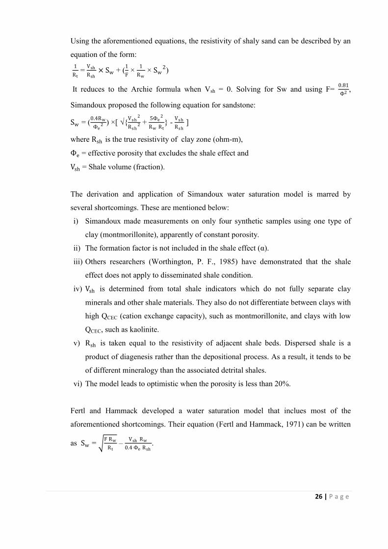
Using the aforementioned equations, the resistivity of shaly sand can be described by an
equation of the form:
1
Rt = Vsh
Rsh× Sw + (1
F × 1
Rw × Sw
2)
It reduces to the Archie formula when Vsh = 0. Solving for Sw and using F= 0.81
Ф2 ,
Simandoux proposed the following equation for sandstone:
Sw = (0.4Rw
Фe2 ) ×[ √{Vsh
2
Rsh2 + 5Фe
2
Rw Rt} - Vsh
Rsh ]
where Rsh is the true resistivity of clay zone (ohm-m), Фe = effective porosity that excludes the shale effect and
Vsh = Shale volume (fraction).
The derivation and application of Simandoux water saturation model is marred by
several shortcomings. These are mentioned below:
i) Simandoux made measurements on only four synthetic samples using one type of
clay (montmorillonite), apparently of constant porosity.
ii) The formation factor is not included in the shale effect (α).
iii) Others researchers (Worthington, P. F., 1985) have demonstrated that the shale
effect does not apply to disseminated shale condition.
iv) Vsh is determined from total shale indicators which do not fully separate clay
minerals and other shale materials. They also do not differentiate between clays with
high QCEC (cation exchange capacity), such as montmorillonite, and clays with low
QCEC, such as kaolinite.
v) Rsh is taken equal to the resistivity of adjacent shale beds. Dispersed shale is a
product of diagenesis rather than the depositional process. As a result, it tends to be
of different mineralogy than the associated detrital shales.
vi) The model leads to optimistic when the porosity is less than 20%.
Fertl and Hammack developed a water saturation model that inclues most of the
aforementioned shortcomings. Their equation (Fertl and Hammack, 1971) can be written
as Sw = F Rw
Rt – Vsh Rw
0.4 Фe Rsh.

27 | P a g e
3) The Indonesia model was developed by field observation in Indonesia rather than by
laboratory experimental measurement support. It remains useful because it is based on
readily available standard log-analysis parameters and gives reasonably reliable results.
The formula was empirically modeled with field data in water-bearing shaly sands, but
the detailed functionality for hydrocarbon-bearing sands is unsupported, except by
common sense and long-standing use. Sw results from the formula are comparatively
easy to calculate and, because it is not a quadratic equation, it gives results that are
always greater than zero. Several of the other quadratic and iterative-solution models can
calculate unreasonable negative Sw results. The Indonesia model (Poupon, and Leveaux,
1971) and other similar models are often used when field-specific SCAL (special core
analysis laboratory) rock electrical-properties data are unavailable but are also sometimes
used where the SCAL exponents do not measure the full range of shale volumes.
Although it was initially modeled on the basis of Indonesian data, the Indonesia model
can be applied everywhere. The inputs are the effective porosity (Фe), shale volume and
resistivity (Vsh and Rsh), formation water and deep resistivities (Rw and Rt). The Sw
output is usually taken to be the water saturation of the effective porosity, but it has been
recently suggested that the output is likely to estimate water saturation of the total
porosity, Swt (Woodhouse, and Warner, 2005). Local experience in the Gulf of Suez for
Wells 1 and 2 showed that the geometric form of the existing shale is a laminated one.
Consequently, the Indonesia equation was used to calculate water saturation in this shaly
sand case. Indonesia equation for water saturation estimation (Poupon et al, 1970;
Hamada, G. M., 1996) is defined as
For un-invaded zones, Sw = ( 1
Rt)[{Vcl
(1−0.5V cl )
Rcl0.5 }+{ Фe
(0.5m )
aR w0.5 }] and
For flushed zone saturation, Sxo = ( 1
Rxo)[{Vcl
(1−0.5V cl )
Rcl0.5 }+{ Фe
(0.5m )
aR mf0.5 }]
4) Waxman-Smits-Thomas and Dual-Water models:
The water saturation of the total porosity (Swt), is calculated at each reservoir data point
by iterative solution of the complex multi parameter Waxman-Smits-Thomas (WST) and
dual-water (DW) equations. The WST and DW models are total-porosity, Sw system
models. The WST model is based on laboratory measurements of resistivity, porosity,
and saturation of real rocks (Waxman and Smits, 1968; Waxman and Thomas, 974). This
equation is expressed as

28 | P a g e
1
Rt = Фt
m∗ SWtn∗ { 1
Rw + BQv
Swt }
where Qv is the cation-exchange capacity (CEC) per unit PV, B = specific cation
conductance in (1/ohm.m)/(meq/mL), and Qv = CEC in meq/mL of total PV. The
exponents m* and n* apply to the total PV. The DW model (Clavier et al., 1984) is also
based on the WST data. It uses clay-bound-water conductivity instead of WST’s BQv
factor and an alternative shale-volume descriptor, Swb (The saturation of physically
bound water in the total PV). When Vsh is zero, Swb is zero; and when Vsh is 100% BV,
Swb and Swt are also 100% PV.
DW model gives the following equation: 1
Rt = Фt
m0 . SWtn0 [ 1
Rwf + Sw h
Swt { 1
Rw h - 1
Rwf }]
where Rwh = resistivity of clay-bound water (RtФtm) in the shales, and Rwf = resistivity
of free formation water in the shale-free water zones. Because of the different model
assumptions, Dual Water exponent mo and no must always be smaller than the WST
exponents (Clavier et al., 1984) and may be values similar to "clean" sand exponents.
3.1.4 Geothermal gradient and formation temperature
Geothermal gradient (Gg) may also be determined by taking pertinent information from
the header and using the following equation (HLS Asia Ltd., 2008):
Gg = [{BHT− Ts
TD}×100] where BHT is the Bottom Hole Temperature in degree Fahrenheit,
Ts is the surface (ambient) temperature in degree Fahrenheit and TD is the Total Depth.
Once the geothermal gradient (Gg) has been established, it is possible to determine the
temperature for a particular depth. This is often referred to as formation temperature (Tf).
As with geothermal gradient, Tf may be determined through the use of charts GEN- 2a or
GEN-2b (HLS Asia Ltd., 2008). It may also be calculated using the following equation:
Tf = [Ts + ( Gs
100× Formation depth].
3.1.5 Formation water resistivity
Formation water (connate water) is the water, uncontaminated by drilling mud that
saturates the porous formation rock. The resistivity of this formation water (Rw) is
important interpretation parameters since it is required for the calculation of saturation
(water or hydrocarbon) from basic resistivity logs by Inverse Archie’s method (Miah and
Howlader, 2012; HLS Asia Ltd., 2008) as below equation: .

29 | P a g e
Formation water resistivity, Rwa = [Rt .ФNDm
a] for un-invaded zone and
Formation mud filtrate resistivity, Rmf = [Rxo .ФNDm
a] for flushed zone.
A more straightforward method of correcting resistivity (ohm-m) for temperature is
through the use of Arp's equation (Asquith, G. and Krygowski, D., 2004):
R2= R1 × (T1+ k
T2+ k)
Where
R2= resistivity value corrected for temperature, T2
R1= resistivity value at known reference temperature, T1
T2= temperature to which resistivity is to be corrected
k= constant value (6.66 for measured temperature in degree Fahrenheit).
3.1.6 Moveable hydrocarbon index
Hydrocarbon movability equation is derived from a comparison of Sw and Sxo. The
greater the difference between Sw and Sxo, the movability is greater (Serra, O., 2007). If
the value for Sxo is much greater than the value for Sw then hydrocarbons were likely
moved during invasion, and the reservoir will produce. An easy way of quantifying this
relationship is through the moveable hydrocarbon index, MHI (= Sw
Sxo). Once flushed zone
water saturation is calculated, it may be compared with the value for water saturation of
the un-invaded zone at the same depth to determine whether or not hydrocarbons were
moved from the flushed zone during invasion. If the value for Sxo is much greater than
the value for Sw, then hydrocarbons were likely moved during invasion, and the reservoir
will produce. When MHI is equal to 1.0 or greater, then this is an indication that
hydrocarbons were not moved from the flushed zone during invasion of mud filtrate
(Asquith, G. and Krygowski, D., 2004; HLS Asia Ltd., 2008).
3.1.7 Bulk volume water
Bulk volume water (BVW) is the product of porosity and water saturation which
represents the percentage of rock volume that is water. Water saturation simply
represents the fraction of porosity in a reservoir that is occupied by water. In some
instances, it may be beneficial to know the fraction of rock volume that is occupied by
water. Bulk volume water has several important applications. Within a particular

30 | P a g e
reservoir, BVW may be calculated at several depths. Where values for BVW remain
constant or very close to constant throughout a reservoir, this may be taken as an
indication that the reservoir is at or near irreducible water saturation (Swirr). Irreducible
water saturation is the value of water saturation at which all water within the reservoir is
either adsorbed onto grain surfaces or bound within the pore network by capillary
pressure. If a reservoir is at irreducible water saturation, then the water present within
that formation will be immovable and production will theoretically be water free
hydrocarbons. Reservoirs that exhibit variation in values for BVW are typically not at
irreducible water saturation and, therefore, at least some water production can be
expected. Swirr is related to the grain size of a reservoir. As grain size decreases, the
diameters of pore throats within the reservoir will decrease, resulting in higher capillary
pressures. This condition implies a reservoir in which a substantial amount of water may
be trapped and unable to move. Therefore, when a reservoir is determined to be at
irreducible water saturation, values for BVW may be used to estimate the average grain
size of that reservoir (Table 3.3). Realizing the potential for error, this approximation
may also be used in reservoirs that are not at irreducible water saturation. The presence
of clay minerals in a reservoir also has an impact on values of irreducible water
saturation and bulk volume water. As the volume of clay minerals in a reservoir
increases, both Swirr and BVW will increase because of the inclination of clay to trap
interstitial formation water. If a reservoir is deemed to be at Swirr, then a log derived
estimate of permeability can be made. Constant to near-constant values of bulk volume
water within a reservoir indicate that reservoir is at (or at least near) irreducible water
saturation (HLS Asia Ltd., 2008).
Table 3.3 Relationship between BVW and grain size in sandstone reservoirs
(Asquith, G. and Krygowski, D., 2004)
Lithology Grain Size (mm) BVW
Coarse 1.0-0.5 0.02-0.025
Medium 0.5-0.25 0.025-0.035
Fine 0.25-0.125 0.035-0.05
Very Fine 0.125-0.062 0.05-0.07
Silt <0.0625 0.07-0.09

31 | P a g e
3.1.8 Log derived permeability
Permeability is the property of a rock that permits the passage of a fluid through the
interconnected pores without damage to or displacement of the rock particles Therefore,
permeability is the measure of the ability of a porous material to transmit fluids. A rock
is termed permeable if an appreciable quantity of fluid can pass through it in a short time
and it is termed impermeable if the rate of passage is negligible. Many rocks are
impervious to movement of water, oil or gas even though they may actually be quite
porous. For example, shales, chalks, clays and some highly cemented sandstones. The
unit of measurement of the permeability of a rock is normally expressed in millidarcys,
or units of one thousandth of a Darcy. A rock has a permeability of 1 Darcy when 1 cm3
per sec of fluid of unit viscosity in centipoises will flow through a section of 1 cm in
length and 1 cm2 in cross section when the difference in pressure on opposite faces is 1
atmosphere. The permeabilities of average reservoir rocks generally range between 5 and
1000 millidarcys (mD). Permeability along with the porosity varies greatly both laterally
and vertically in the average reservoir rock. A reservoir rock whose permeability is 5 md
or less is called a tight sand or dense limestone according to its composition. The
permeability of a reservoir can be measured in three ways as drill stem or production test,
permeameter (laboratory test) and wireline logs (Shelly, 1987). If a reservoir is deemed
to be at irreducible water saturation, then a log derived estimate of permeability (KL) can
be made. Wyllie and Rose method (Crain, E. R., 1986) of permeability determination as
KL = [ (CPERM × ФDPERM )
(SwirrEPERM )
2
] in mD for dry gas
Where
Ф = Porosity and
Sw,irr is the water saturation (Sw) of zone assumed to be at an irreducible.

32 | P a g e
CHAPTER FOUR
RESULTS AND DISCUSSIONS
Bakhrabad well no. 9 (BK#9) has been selected for the current research purpose where available
log data is listed in Table 4.1. The quality of all log data is good except SP log. SP log has not
been used in this study. In the studied well, no depth shift has been found in the logs. No
environmental corrections are applied to the aforementioned logs. The potassium (percentage),
thorium and uranium (ppm) have been taken from spectral gamma ray log. The Gamma Ray API
value is taken from natural Gamma Ray log.
Table 4.1 Available log data of BK#9
Log type Log Name
Borehole measurement log Caliper log with Bit size
Lithology logs Spectral and Natural Gamma Ray log
Self-Potential (SP) log
Porosity logs Spectral density, Dual spaced Neutron, and Sonic Log
Resistivity logs Array compensated true resistivity
(Shallow and Deep Resistivity logs)
4.1 Lithology and Hydrocarbon Bearing Zones
Logging parameters have been taken from log header of the studied well that is shown in
Table 4.2. Log reading on each available log curve has been taken with respect to depth
and then analyzed. The true resistivity of virgin zone is higher than the shallow zone’s
resistivity in the sand zone in Figure 4.1. The caliper curve shows mud-cake in the sand
zone. This mud-cake indicates that the sand zone is porous and permeable. Cross over is
showing between Neutron and density logs through the hydrocarbon bearing sand zone
in Figure 4.2. There are six hydrocarbon (gas) bearing sand zones found from 2042 m to
2500.5 m (True Vertical Depth-TVD) based on GR log, resistivity log and porosity logs.
Among them, one is thick sand from 2120 m to 2138 meter depth.

33 | P a g e
Table 4.2 Logging parameters of BK#9
Mud Parameters Value
Location (m) Lat.: 23036´53.31´´ N, Long.: 90052´45.26´´ E
Drillers depth (TVD) 3535 m
Logger depth (TVD) 2532.7 m
Logged Interval (Top & Bottom) 1707.5 m and 2532.06 m
Casing-Diller 9.625 in @ 1709 m
Kelly Bushing Elevation (m) 7.32
Bit Size (Inch) 8.5
Type of Fluid LSND Polymer
Density & PH 1.14 g/cc and 9.50
Rm and Rmf (Ω-m) 0.80 and 0.75 @800F
BHT & Depth 280 0F @ 2532.7 m
Figure 4.1 Resistivity log including lithology log of hydrocarbon bearing thick sand
Hydrocarbon bearing sand
SP Log
GR Log
Shale (Cap rock)
Shale
Rt
Rxo
1.0 Ω-m 10 100 100 0 API

34 | P a g e
Figure 4.2 Cross-over of thick sand between spectral density and neutron porosity logs
The raw data of different well logs of hydrocarbon bearing zones of BK#9 is shown in
Appendix-A1 through A5. The radioactive properties, formation resistivity with bulk
density and neutron porosity of six sands are shown in Table 4.3 for BK#9. The true
formation resistivity (Rt) and flushed zone resistivity, Rxo (ohm-m) have been taken from
deep and shallow resistivity logs of this well. The bulk density (RHOb), photoelectric
absorption cross section (Pe) and neutron porosity (NPHI) are taken from litho-density
and neutron porosity logs, respectively. According to log data analysis of drilled well, the
lithology is mainly sand and shale where sand is the dominant fraction. Clay type is
Kaolinite (Pe=3.17 from litho-density log) and Shales are laminated. The average bulk
density of the six gas bearing sands are found from the litho-density log as 2.37-2.46
gm/cc. The Thorium and Uranium minerals of six sands are 10.761-13.843 ppm and
1.702-2.7 ppm, respectively. Total thickness of thick gas bearing sand reservoir is 18 m
which is located at the depth of 2120 m to 2138 m. The depth of all hydrocarbon bearing
zones are located in Bokabil Formation of Bengal Basin (RPS Energy, 2009a; IKM,
1990a). A graphical representation of depth versus radioactive properties minerals of
thick sand is shown in Figure 4.3.
ρb φN
CALI

35 | P a g e
Table 4.3 Values of formation radioactive minerals, bulk density, resistivity and others
Parameters Thin
sand-1
Thin
sand-2
Thick
sand-1
Thin
sand-3
Thin
sand-4
Thin
sand-5
Top-Base (TVD),
meter
2042-
2045
2100-
2102
2120-2138 2150.5-
2156.5
2363-
2368
2498.5-
2500.5
Normal GR (API) 96.00 102.00 99.00 105.00 103.00 111.00
Th (ppm) 11.407 12.786 12.340 13.843 12.833 10.761
U (ppm) 2.287 2.298 2.248 1.990 2.459 2.700
K (%) 1.506 1.532 1.702 1.855 1.657 1.413
Rt (ohm-m) 14.00 17.00 16.00 22.80 12.90 17.00
RHOb (g/cc) 2.35 2.35 2.39 2.42 2.33 2.46
NPHI (%) 24.50 19.00 17.33 16.47 16.50 12.55
Pe (barns/electron) 3.12 3.23 3.17 3.34 2.92 3.53
DELT (μs/ft) 96.39 86.33 92.90 85.26 70.05 83.68
Figure 4.3 Radioactive properties with formation depth of thick sand reservoir
4.2 Estimation of Shale Volume and Reservoir Thickness
The maximum abundance of radioactive minerals as Thorium (Thmax) and Potassium
(Kmax) from spectral natural gamma ray log within the formation is 19.231 ppm and
2.818%, respectively at 2405 m (TVD). On the other hand, Kmin and Thmin are 1.315
0.52.54.56.58.5
10.512.514.516.518.5
21
20
21
21
21
22
21
23
21
24
21
25
21
26
21
27
21
28
21
29
21
30
21
31
21
32
21
33
21
34
21
35
21
36
21
37
21
38
Rad
ioac
tive
prop
ertie
s (pp
m)
Formation Depth (meter)
URAN THOR
36 | P a g e
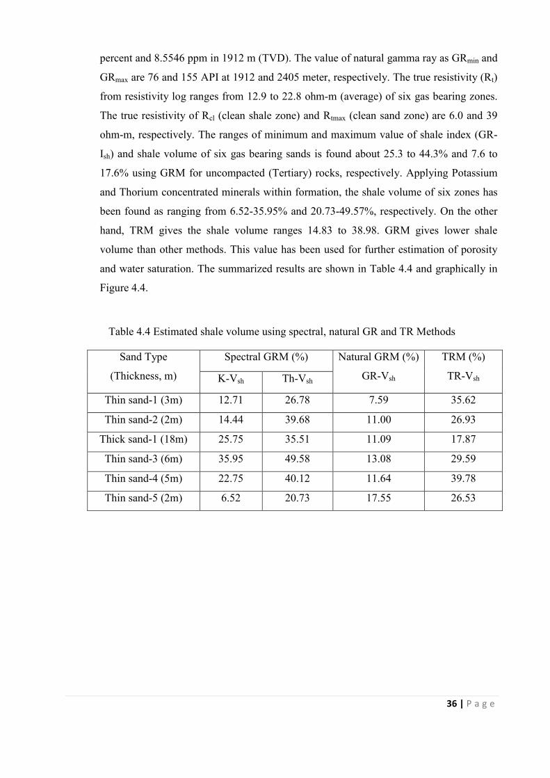
percent and 8.5546 ppm in 1912 m (TVD). The value of natural gamma ray as GRmin and
GRmax are 76 and 155 API at 1912 and 2405 meter, respectively. The true resistivity (Rt)
from resistivity log ranges from 12.9 to 22.8 ohm-m (average) of six gas bearing zones.
The true resistivity of Rcl (clean shale zone) and Rtmax (clean sand zone) are 6.0 and 39
ohm-m, respectively. The ranges of minimum and maximum value of shale index (GR-
Ish) and shale volume of six gas bearing sands is found about 25.3 to 44.3% and 7.6 to
17.6% using GRM for uncompacted (Tertiary) rocks, respectively. Applying Potassium
and Thorium concentrated minerals within formation, the shale volume of six zones has
been found as ranging from 6.52-35.95% and 20.73-49.57%, respectively. On the other
hand, TRM gives the shale volume ranges 14.83 to 38.98. GRM gives lower shale
volume than other methods. This value has been used for further estimation of porosity
and water saturation. The summarized results are shown in Table 4.4 and graphically in
Figure 4.4.
Table 4.4 Estimated shale volume using spectral, natural GR and TR Methods
Sand Type
(Thickness, m)
Spectral GRM (%) Natural GRM (%)
GR-Vsh
TRM (%)
TR-Vsh K-Vsh Th-Vsh
Thin sand-1 (3m) 12.71 26.78 7.59 35.62
Thin sand-2 (2m) 14.44 39.68 11.00 26.93
Thick sand-1 (18m) 25.75 35.51 11.09 17.87
Thin sand-3 (6m) 35.95 49.58 13.08 29.59
Thin sand-4 (5m) 22.75 40.12 11.64 39.78
Thin sand-5 (2m) 6.52 20.73 17.55 26.53

37 | P a g e
Figure 4.4 Shale volume versus formation depth of thick sand
The aforementioned result shows that the shale volume changed causes for changing the
radioactive minerals (Thorium Uranium and Potassium concentration) within formation
(Total GR value) with respect to depth. From GR method, estimated arithmetic average
shale volume of thick sand is found about 11.09 percent which is almost close to
estimated shale volume (8%) by IKM, 1991 (G sand: 2084-2140m TVD, BK#3). The
gross thickness of thick sand is 18m (2120-2138m) where net thickness is 17m. The Net
to Gross ratio has been estimated to be 0.94 based on spectral and natural GR log.
4.3 Assessment of Porosity
Porosity has been estimated from single log methods as well as from Neutron-Density
combination formula. In this method, individual porosity from Neutron, Density and
Sonic logs have been calculated and compared with each other. In order to interpret and
analyse the log data, matrix travel time (∆Tma) of 55.5µs/ft and matrix density (ρma) of
2.65gm/cc (Schlumberger, 1998a) has been used for porosity assessment in sandstone
reservoir. The fluid density (ρf) of 1.0 gm/cc and fluid travel time (∆Tf) of 189µsec/ft
(Schlumberger, 1998a) has been used for porosity estimation. On the other hand,
adjacent shale neutron porosity of 16% is used for porosity estimation. The estimated
porosity results are shown in Appendix-C1 and C2. The summarized results of porosity
are shown in Table 4.5 and graphically represented in Figure 4.5. Formation evaluation is
0.00
10.00
20.00
30.00
40.00
50.00
60.00
70.00
80.00
90.00
2120 2122 2124 2126 2128 2130 2132 2134 2136 2138
Shal
e V
olum
e, V
sh (%
)
Formation Depth (meter)
Potassium Thorium NGR TRM

38 | P a g e
made by using cutoff shale volume (GRM-Vsh), effective porosity and water saturation
of 40%, 8%, and 60%, respectively. The aforementioned cut off values is taken from the
previous log interpretation report (RPS Energy, 2009c).
Table 4.5 Estimated porosity from Neutron, Density and Sonic logs
Sand Name Thin
sand-1
Thin
sand-2
Thick
sand-1
Thin
sand-3
Thin
sand-4
Thin
sand-5
NPH (%) 24.50 19.00 17.33 16.47 16.50 12.55
PHID (%) 19.09 18.18 17.22 14.10 19.39 11.52
PHIN-D (%) 21.96 18.60 17.36 15.33 11.52 12.04
PHIN-De (%) 20.79 16.87 15.64 13.28 16.18 9.28
PHIs 30.63 23.09 28.02 22.29 10.90 21.11
Φsonic , gas (%) 21.44 16.16 19.61 15.60 7.63 14.78
Figure 4.5 Depth versus average porosity of thick sand reservoir
The sonic log generally gives higher porosity because of gas effects. The total porosity
from sonic log is 28.02% but corrected sonic porosity for gas effect is 19.61% by Hilchie
formula in thick sand reservoir. Among gas sands, the arithmetic average neutron and
density porosity ranges are 12.55-24.50% and 11.52-19.39% respectively, but neutron
7.00
9.00
11.00
13.00
15.00
17.00
19.00
21.00
23.00
25.00
21
20
21
21
21
22
21
23
21
24
21
25
21
26
21
27
21
28
21
29
21
30
21
31
21
32
21
33
21
34
21
35
21
36
21
37
21
38
Po
rosi
ty (
%)
Formation Depth (meter)
NPHI PHID PHI_NDe

39 | P a g e
and density combination formula gives 12.04 to 21.96 % porosity. The estimated
porosity using clay corrected neutron-density combination formula is 9.28 to 20.79 % for
gas bearing reservoir. This porosity quality is good for this gas pools.
4.4 Geothermal Gradient and Formation Temperature
The determined geothermal gradient and formation temperature of the studied well is
shown in Appendix-E1. From the log data analysis, it is found that the geothermal
gradient is 3.948 0F per 100 meter of BK#9 with average formation temperature of thick
sand depth interval of 163.71 to 164.42 0F. From the analysis, it is found that this (2120-
2138m TVD) well shows lower geothermal gradient compared with 5.91 0F per 100m of
G sand (IKM, 1990a). The geothermal gradient and formation temperature are varied
with respect to depth of the formation.
4.5 Formation Water Resistivity
As stated earlier that formation water resistivity (Rw) has been calculated from Inverse
Archie’s method (Rwa analysis) where tortousity factor (a) of 1.00 and cementation
exponent (m) of 2.25 (IKM, 1990a) has been used. The data has been taken from several
water bearing sands of the well for Rwa analysis (Appendix-D). The minimum value of
Rw is 0.104 and mud-filtrate resistivity (Rmf) is 0.157 ohm-m has been found in interval
from 1960 to 1969 meter (TVD). Finally considering this interval, Rw and Rmf have been
calculated for others gas bearing sands and then corrected for formation temperature with
respect to depth. Thus a profile of Rw and Rmf are prepared and water saturation is
estimated for each thin and thick gas sands level (Appendix-E1). Salinity of thick sand
interval has been estimated using Chart Gen-9 (Schlumberger, 1998b). The average
formation water resistivity has been found as 0.10 ohm-m by Rwa analysis and formation
salinity is about 29000 ppm of NaCl at 164 0F. The surface salinity is 32000 ppm of
NaCl with respect to Rw of 0.197 ohm-m at 80 0F using Chart Gen-9 in Appendix-E2.
The field measured resistivity is 0.38 ohm-meter at 760F with a NaCl content of 15,000
ppm and 0.2 ohm-m at 175 0F by IKM, 1990a. The mud filtrate resistivity (Rmf) has also
been estimated in the same way for studied well and shown in Appendix-E1.

40 | P a g e
4.6 Determination of Water Saturation
The tortousity (a), saturation (n) and cementation exponent (m) value of 1.00, 2.00 and
2.00 has been used for water saturation estimation for both thick and thin sands of this
well, respectively (Schlumberger, 1998a). Estimated water saturation is shown in Table
4.6 for gas bearing sands, and graphical representation is also shown in Figure 4.6. The
detailed results are shown in Appendix-F1, F2 and F3.
Table 4.6 Estimated water saturation from different models
Sand type
Thickness
(meter)
Archie’s formula
(average, %)
Indonesia model
(average, %)
Simandoux model
(average, %)
Swa Sxoa Swi Sxoi Sws
Thin sand-1 3 13.12 22.34 39.02 56.92 36.71
Thin sand-2 2 14.47 25.98 41.64 64.09 40.77
Thick sand-1 18 14.26 27.60 39.18 70.96 40.30
Thin sand-3 6 18.74 30.15 51.84 77.83 53.05
Thin sand-4 5 16.31 24.63 48.05 65.09 47.36
Thin sand-5 2 24.08 37.12 62.31 99.54 71.21
Figure 4.6 Average water saturation of thick sand of different models
10.0015.0020.0025.0030.0035.0040.0045.0050.0055.0060.00
2120
2121
2122
2123
2124
2125
2126
2127
2128
2129
2130
2131
2132
2133
2134
2135
2136
2137
2138
Wat
er S
atur
atio
n, S
w (%
)
Formation Depth (meter) of thick reservoir sand
Archie's Indonesia Simandoux

41 | P a g e
From the Archie’s equation, it is found that highest water saturation is about 29.3% at a
depth of 2128m and the lowest value is about 9.8% at 2136m of thick sand. These
highest and lowest saturation values are also confirmed by Indonesia and Simandoux
model as shown in Figure 4.6. From Simandoux model, estimated water saturation is
found about 89% in Figure 4.6 at 2128m depth because of shale effect. The maximum to
minimum value of hydrocarbon (gas) saturation from Archie’s formula, Simandoux and
Indonesia models are 86.88-75.92, 63.29-28.79 and 60.98-37.69 percent, respectively.
Indonesia equation and Simandoux model give more reliable saturation value than
Archie’s formula because this reservoir is almost shaly sand reservoir. On the other hand,
Archie’s formula gives better estimation of water saturation for clean sand reservoirs of
any formation. This fluid saturation is most important for reserve estimation and
reservoir data analysis of this well.
4.7 Moveable Hydrocarbon Index and Bulk Volume Water
The average moveable hydrocarbon index (MHI) of six reservoir sands ranges are 0.52 to
0.66 by Archie’s formula and 0.57 to 0.74 from Indonesia equation which is an
indication that hydrocarbons were moved from the flushed zone during invasion of mud
filtrate. So, hydrocarbon is moveable within thick and thin sands reservoir of this
formation. The BVW (Product of porosity and water saturation) has been estimated from
Archie’s formula, and Indonesia - Simandoux model’s water saturation of gas sands
which ranges from 0.021 to 0.027, 0.058 to 0.081 and 0.063-0.077, respectively. Detailed
results of MHI and BVW are shown in Appendix- F1, F2 and F3. These values are
indicating that the grain size of this reservoir sand is coarse to medium and very fine,
respectively (After Asquith, G. and Krygowski, D., 2004).
4.8 Log Derived Permeability
The permeability of the reservoir sand has been calculated using Wyllie & Rose equation
assuming irreducible water saturation, Swirr of 18%, permeability constant (CPERM) of
8581 (RPS Energy, 2010), irreducible saturation exponent (EPERM) of 2.00, and
porosity constant (DPERM) of 4.40, respectively (IKM, 1990a). Using the above
parameters, the average log derived permeability ranges from 7.59 to 263.90 mD by
Wyllie and Rose method of six reservoir sands. Among gas bearing sands, the minimum,
maximum and average values of permeability are 5.07, 85.45 and 221.99 mD,

42 | P a g e
respectively for thick sand reservoir. Detailed result of gas bearing reservoir permeability
is shown in Appendix-G.
4.9 Comparison of Petrophysical Properties with Different Studies
The petrophysical properties of thick gas bearing reservoir (local named as G sand) of
BK Field (BK#1 to BK#9) including the current studied well in a tabular form is shown
in Table 4.7.
Table 4.7 A comparison of petrophysical properties of different wells (thick sand)
Parameters/
Properties
IKM, 1991
RPS
Energy,
2009
(P10 to
P90)
Current
Study
Well No. BK#
1
BK#
2
BK#
3
BK#
4
BK#
5
BK#
6
BK#
7
BK#
8
BK#
1-8
BK#9
G or Thick
sand
interval, ft
(TVD)
6850
-
7030
6920
-
7000
6840
-
7020
6920
-
7000
6960
-
7103
6920
-
7100
6820
-
7000
6912
-
7028
7813 –
8826
(MD)
6953
-
7013
Net Pay, ft 49.5 74.5 81.5 58.0 100 59.5 89.0 61.5 32.5- 144 63
Vsh (%) 18.0 23.0 11.0 17.0 - 19 20.0 18.0 8.5-32.0 11.0
Фe (%) 19.8 16.8 21.6 20.0 - 15.7 16.7 19.0 13.6 -21.2 15.6
Sw (%) 26.8 26.2 37.5 27.9 - 35.5 31.0 25.9 18.4 - 37.8 39.1
Rw (Ω-m) 0.2 at 1750F 0.2 at
1750F
0.1 at
1640F
Rt (Ω-m) 30-70 N/A 17-38
KL (mD) 109.4 (BK#2) and 98.8 mD (BK#3) from Production
Test Data
61.3
-
219.3
34.2
-
222.0
MHI N/A N/A 0.57
BVW N/A N/A 0.06

43 | P a g e
4.10 Justification and Uncertainty of the Results
The available logs are interpreted and analyzed using different methods and different
approaches. Each method has some limitations in their applicability. Some uncertainties
are also there in assumption and application for formation evaluation of this well. Some
error may also be there in picking the correct log values. However, uncertainty on logs as
well as on the analytical procedure has been described under the following headings:
Shale volume: This may be changed due to heterogeneity of radioactive minerals
within the formation.
Porosity assessment: Single log porosity method and Neutron-Density combination
formula have been used for porosity estimation. Individual porosity logs give big
differences of porosity values. Cross-Plot method (gives best result other than core)
could not be followed as pure water bearing zones are uncommon in the studied well.
The assumed values of both fluid and matrix density, and travel time may be changed
due to inhomogeneity of the lithology. Porosity from core analysis is more reliable
than the aforementioned methods.
Formation water resistivity and selection of exponents: The water bearing clean
sands are uncommon in the studied well. As a result, the estimation of corrected Rw
may be wrong due to changing of cementation exponent (m) and actual sub-surface
formation temperature. This is an important parameter for estimation of formation
water saturation. These exponents (a=1, m=2 and n=2) are critical in calculating
porosity, formation water resistivity and water saturation of flushed zones as well as
un-invaded zones.

44 | P a g e
CHAPTER FIVE
CONCLUSIONS AND RECOMMENDATIONS
5.1 Conclusions
Based on the log interpretation and formation evaluation using available wireline log
data for BK#9 well, the conclusions are as follows:
Thick gas bearing sand (G sand) is the main reservoir of this well where lithology is
mainly medium to coarse grained sand with subordinate shale of laminar type. The
average Gamma Ray and resistivity ranges are 96-111 API and 13-23 ohm-m of
reservoir sands where shale content is about 11 and 18 % from Natural Gamma Ray
and True resistivity methods of thick sand, respectively.
Neutron-Density combination formula gives better effective porosity value of shaly
sand reservoirs which is about 9.28-20.79 % as compared to the single log method.
This is good quality porosity of this formation.
Log analysis shows that the average formation water resistivity (Rw) of thick gas
bearing sand is 0.10 ohm-m from Rwa analysis and formation salinity is about 29000
ppm of NaCl and surface salinity is about 32000 ppm (NaCl) with Rw of 0.197 ohm-
m.
Simandoux and Indonesian model give a pessimistic value of water saturation of
virgin zone in thick sand as 40 and 39%, respectively compared with the Archie’s
formula (14%). The first two saturation methods are more reliable for shaly sand
reservoir and they also match with earlier interpretations. Thus, average gas
saturation of thick sand is found to be about 60% at depth interval 2120-2138m
(TVD). Gas is also moveable within thick and thin sands reservoir of this reservoirs
or formation. The estimated log derived average permeability from Wylie-Rose
method has been estimated as 34-222 mD which is a good permeability for sand
reservoirs. So the gas pools of this formation are potential for production gas.

45 | P a g e
5.2 Recommendations
Bakhrabad field is one of the onshore gas fields of Bangladesh. From the current study of
the available log data of this gas field, the following recommendations may be drawn:
In order to assess the quality of the reservoir sands of variable thickness, whether it is
thick or thin, this field should be given careful attention in the light of formation
evaluation with data from new drilled wells.
To estimate the water saturation of a reservoir, the special or routine core analysis is
required. The estimated reservoir thickness, porosity and hydrocarbon saturation can
be used for future reserve estimation and reservoir properties analysis of this
formation.
To assess the quality of the gas reservoirs of Bangladesh accurately, special logging
tools such as Nuclear Magnetic Resonance (NMR) and Formation Micro-Scanner
(FMS) logs can be run with conventional wire line logs.
All the nine wells drilled so far in this structure are mainly located to the northern part
of the structure. To date, no wells has been drilled in the flank of the structure that
could tell the extension and quality of the reservoir as well as its gas saturation,
presence of fluid contact (GWC), and minimize the uncertainty of estimation of
hydrocarbon reserve. Additional wells may be drilled in the southern end part of the
structure for better picture of the lithology of this gas field.

46 | P a g e
REFERENCES
Akhanda, A. R., and Islam, Q., 1994, Introduction to Petroleum Geology and Drilling,
Publication-cum-Information Office, Bangladesh, p. 78.
Archie, G. E., 1942, The Electrical Resistivity Log as an Aid in Determining Some
Reservoir Characteristics, Trans. of AIME Transactions, V. 146 (1), p. 54-67.
http://dx.doi.org/10.2118/942054-G.
Asquith, G., and Krygowski, D., 2004, Basic well log analysis, American Association of
Petroleum Geologists, Second Edition, Tulsa, Oklahoma, p. 216.
Bakhrabad Gas Field, 1993, Reservoir Engineering Report Based on 1992 and 1993 Pressure
Surveys-Reservoir Study Unit, PIU & BAPEX, Petrobangla, Bangladesh Gas Fields
Company Limited (BGFCL) Library.
BGFCL, 2009, Main Gas Reserves of Different Gas Fields Under BGFCL, Reservoir
Engineering Section, Bangladesh
Bassiouni, Z., 1994, Theory, Measurement and Interpretation of Well Logs, First Printing,
Henry L. Doherty Memorial Fund of AIME, SPE, Richardson, TX, p. 372.
Bateman, R. M., 1985, Open Hole Log Analysis and Formation Evaluation: IHRDC
Publishers, Boston MA, p. 647.
Beaumont A. E. and Foster H. N., 1999, Hand Book of Petroleum Geology, American
Association of Petroleum Geologists, Tulsa, Oklahoma, p. 45-63.
Choudhury, Z., 1999, Reservoir Engineering Study of Bakhrabad Gas Field, M. Sc. Thesis,
PMRE Dept., Bangladesh University of Engineering and Technology (BUET).
Choudhury, Z. and Gomes, E., 2000, Material Balance Study of Gas Reservoirs by Flowing
Wellhead Method: A Case Study of Bakhrabad Gas Field, SPE Asia Pacific Oil and Gas
Conference and Exhibition in Brisbane, Australia, SPE 64456, October 2000, pp. 16-18.
Clavier, C., Coates, G., and Dumanoir, J., 1984, Theoretical and Experimental Bases for the
Dual-Water Model for Interpretation of Shaly Sands, SPE Journal- 24 (2), pp. 153-168,
http://dx.doi.org/10.2118/6859-PA. SPE-6859-PA.
Crain, E. R., 1986, The Log Analysis Handbook, Volume-1, Quantitative Log Analysis
Methods, PennWell Publishing Company, Tulsa, Oklahoma, USA, p. 328.
De Witte, A. j., 1957, Saturation and Porosity From Electric Logs in Shaly Sands, Oil & Gas
Journal, March 1957, pp. 89-93.
Dresser Atlass, 1982, Well Logging and Interpretation Techniques, Dresser Ind. Inc.

47 | P a g e
Darling, T., (2005), Well Logging and Formation Evaluation, Gulf Professional Publishing,
p.326.
Fertl, W.H. and Hammack, C.W., 1971, A Comparative Look at Water Saturation in Shaly
Pay Sand, in 12th Annual Logging Symposium Transaction: Society of Professional
Logging Analysts.
Hamada, G. M., 1996, An integrated Approach to determine shale volume and hydrocarbon
potential in shaly sand, 1996 SCA Conference Ppaer Number 9641. pp. 1-16.
Hilchie, D. S., 1982, Applied Open Hole Log Interpretation for Geologist and Engineers:
Douglas W. Hilchie Inc., Golden Colorado.
HLS Asia Limited, 2008, Basic Log Interpretation, p. 106.
Kobesh, F. P. and Blizard, R. B., 1959, Geometric Factors in Sonic Logging: Geophysics,
v.24, pp. 64-76.
Poupon,A., Clavier, C, Dumanoir,J., Gaymard,R. and Misk, A., 1970, Log Analyses of
Sand-Shale Sequences-A Systematic Approach, Journal of Petroleum Technology, July
1970, p. 867-881.
Poupon, A. and Leveaux, J., 1971, Evaluation of Water Saturations in Shaly Formations,
The Log Analyst-12 (4).
Interkomp Kanata Management (IKM), 1991a, Geological, Geophysical and Petrophysical
Report of Bakhrabad Gas Field, Petrobangla, Bangladesh, p. 88.
IKM, 1991b, Reservoir Engineering Report of Bakhrabad Gas Field, Petrobangla
Bangladesh, p. 92.
Imam, B., 2013, Energy Resources of Bangladesh, Second Edition, University Grants
Commission Publication No. 151, Bangladesh, 2013, p. 324.
Miah, M. Islam and Howlader, M. F., 2012, Prediction of Formation Water Resistivity from
Rwa Analysis of Titas Gas Field Using Wireline Log Data, Journal of Petroleum and Gas
Exploration Research (JPGER), Vol. 2(4), p. 57-60.
RPS Energy, 2009a, Bakhrabad Geological Study, Petrobangla, Dhaka, Bangladesh, p. 50.
RPS Energy, 2009b, Bakhrabad Geophysics Report, Petrobangla, Dhaka, Bangladesh, p. 81.
RPS Energy, 2009c, Bakhrabad Petrophysical Report, Petrobangla, Dhaka, Bangladesh, p.
109.
RPS Energy, 2009d, Bakhrabad Petroleum Engineering Report, Dhaka, Bangladesh, p. 61.
Schlumberger, 1998a, Log Interpretation Principles/Applications, 7th printing, Houston, p.
235.

48 | P a g e
Schlumberger, 1998b, Log Interpretation Charts, Schlumberger Well Services, Houston, p.
65.
Shelly, R.C., 1998, Elements of Petroleum Geology, Academic Press. London, p. 470.
Serra, O., 2007, Well Logging and Reservoir Evaluation, ISBN: 978-2-7108-0881-7, p. 250.
Simandoux, P., 1963, Measures dielectrique en milieu poreus, application a measure de
saturation en eau, etude des massifs argileaux, Revue de I’ ins. Francais du Petrole,
(Supplementary Issue, 1963), p. 193-215.
Waxman, M. H., and Smits, L. J. M., 1968, Electrical Conductivities in Oil-Bearing Shaly
Sands, SPE Journal- 8 (2), pp. 107–122, SPE-1863-PA. http://dx.doi.org/10.2118/1863-PA.
Waxman, M. H. and Thomas, E. C., 1974, Electrical Conductivities in Shaly Sands-I, The
Relation Between Hydrocarbon Saturation and Resistivity Index-II. The Temperature
Coefficient of Electrical Conductivity, Journal of Petroleum Technology, 26 (2), pp. 213-
225. http://dx.doi.org/10.2118/4094-PA.
Welldrill (UK) Ltd., 1983, Final Well Report, Bakhrabad Wells (BK-1, 2, 3 4 and 5).
Woodhouse, R. and Warner, H. R., 2005, Sw and Hydrocarbon Pore Volume Estimates in
Shaly Sands- Routine Oil-Based-Mud Core Measurements Compared With Several Log
Analysis Models, Presented at the SPE Annual Technical Conference and Exhibition,
Dallas, Texas, 9-12 October 2005. http://dx.doi.org/10.2118/96618-MS.
Worthington, P. F., 1985, The Evaluation of Shaly Sand Concepts in Reservoir Evaluation,
The Log Analyst-24, No. 1.
Wyllie, M. R. J, Gregory, A. R., and Gardner, G. H.F, 1956, Elastic Wave Velocity in
Heterogeneous and Porous Media, Geophysics-21, January 1956, pp. 41-70.

49 | P a g e
Appendix-A1: Lithology and Resistivity logs of BK#9
Thin sand-1 (2042-2045 m

50 | P a g e
Appendix-A2: Spectral and natural GR logs of thin sand-1 reservoir
Thin sand-1 (2042-2045 m

51 | P a g e
Appendix-A3: Spectral density, Dual spaced neutron and GR logs
Thin sand-1 (2042-2045 m

52 | P a g e
Appendix-A4: Borehole compensated sonic array log of BK#9
Thin sand-1 (2042-2045 m

53 | P a g e
Appendix-A5: Raw data from different logs for formation evaluation
Thick sand reservoir (BK#9)
Depth interval Lithology Logs Resistivity logs Porosity logs CALI Top Bottom THOR POTA URAN GR Rt Rxo 𝛒𝐛 NPHI Pe DET Hole, d
meter meter ppm % ppm API ohm-meter g/cc % b/elec. µs/ft inc. 2119 2120 13.444 1.672 3.193 110.0 23.0 15.0 2.38 15.68 3.26 87.55 8.35 2120 2121 12.444 1.542 2.806 100.0 20.0 12.0 2.39 18.02 3.29 92.80 8.33 2121 2122 12.887 1.689 2.688 107.0 24.0 12.5 2.33 16.67 3.07 93.28 8.31 2122 2123 12.490 1.716 1.682 97.0 22.5 12.0 2.33 16.66 2.91 93.38 8.32 2123 2124 11.698 1.680 1.425 87.0 24.5 14.0 2.40 24.56 3.13 92.58 8.32 2124 2125 13.030 1.968 1.891 103.0 17.0 11.0 2.39 17.85 3.11 93.68 8.33 2125 2126 15.038 2.066 2.536 118.0 16.5 11.0 2.41 18.99 3.26 90.85 8.34 2126 2127 14.476 1.783 1.250 103.0 20.5 12.5 2.38 17.04 3.10 91.73 8.33 2127 2128 17.429 2.092 2.827 135.0 14.0 9.5 2.46 18.87 3.67 85.84 8.34 2128 2129 12.746 1.601 1.747 97.0 18.5 12.0 2.36 17.31 3.18 93.86 8.33 2129 2130 11.252 1.552 1.849 88.0 20.5 12.0 2.88 17.25 3.34 96.80 8.32 2130 2131 12.821 1.736 2.182 95.0 28.0 15.0 2.38 17.37 3.51 97.15 8.31 2131 2132 12.057 1.709 2.246 103.0 27.5 13.5 2.35 15.96 3.13 93.70 8.31 2132 2133 9.602 1.485 1.942 80.0 25.0 13.5 2.34 15.65 3.11 97.14 8.32 2133 2134 9.208 1.618 2.105 86.0 24.5 13.5 2.33 16.17 3.21 96.05 8.32 2134 2135 9.760 1.620 2.399 87.0 27.5 14.0 2.36 16.19 3.15 92.83 8.32 2135 2136 11.016 1.608 2.522 95.0 38.0 18.0 2.32 16.06 2.90 91.63 8.33 2136 2137 11.966 1.670 2.868 103.0 24.0 24.5 2.34 16.15 3.06 91.46 8.33 2137 2138 11.105 1.530 2.546 91.0 17.0 13.0 2.35 16.74 2.90 92.85 8.34 Arith. Average 12.340 1.702 2.248 99.2 22.8 13.6 2.39 17.33 3.17 92.90 8.33
Thin sand reservoir (meter) TVD
Top Bottom THOR POTA URAN GR Rt Rxo 𝛒𝐛 NPHI Pe DET Hole, d 2042 2045 11.407 1.506 2.287 96.0 14.0 11.0 2.35 24.50 3.12 96.39 8.29 2100 2102 12.786 1.532 2.298 102.0 17.0 13.0 2.35 19.00 3.23 86.33 8.25
2150.5 2156.5 13.843 1.855 1.990 105.1 16.0 14.0 2.42 16.47 3.34 85.26 8.35 2363 2368 12.833 1.657 2.459 103.0 12.9 12.9 2.33 16.50 2.92 70.05 8.33
2498.5 2500.5 10.761 1.413 2.700 111.0 17.0 16.3 2.46 12.55 3.53 83.68 8.45

54 | P a g e
Appendix-B1: Shale volume estimation from Gamma Ray and True Resistivity methods
Thick sand Vsh from Gamma Ray log Vsh from True resistivity method
Depth, m GRlog Calculated Log values (ohm-m) Shale Volume API Ish Vsh (%) Rtmax Rt Rclay Vsh (%)
2120 110 0.430 16.73 39 23 6 16.10 2121 100 0.304 9.79 39 20 6 20.76 2122 107 0.392 14.41 39 24 6 14.78 2123 97 0.266 8.11 39 22.5 6 16.80 2124 87 0.139 3.56 39 24.5 6 14.15 2125 103 0.342 11.64 39 17 6 26.93 2126 118 0.532 24.15 39 16.5 6 28.17 2127 103 0.342 11.64 39 20.5 6 19.90 2128 135 0.747 48.05 39 14 6 35.62 2129 97 0.266 8.11 39 18.5 6 23.61 2130 88 0.152 3.95 39 20.5 6 19.90 2131 95 0.241 7.08 39 28 6 10.30 2132 103 0.342 11.64 39 27.5 6 10.80 2133 80 0.051 1.15 39 25 6 13.55 2134 86 0.127 3.18 39 24.5 6 14.15 2135 87 0.139 3.56 39 27.5 6 10.80 2136 95 0.241 7.08 39 38 6 1.53 2137 103 0.342 11.64 39 24 6 14.78 2138 91 0.190 5.21 39 17 6 26.93
Average 99.21 0.294 11.09 39 22.76 6 17.87
Thin sands reservoir (BK#9)
Depth, m Vsh from Gamma Ray log Vsh from True resistivity method
Top GRlog Calculated Log values (ohm-m) Shale volume
API Ish Vsh (%) Rtmax Rt Rclay Vsh (%) 2042 96.0 0.253 7.59 39 14.0 6 35.62 2100 102.0 0.329 11.00 39 17.0 6 26.93
2150.5 105.1 0.369 13.08 39 16.0 6 29.59 2363 103.0 0.342 11.64 39 12.9 6 39.78
2498.5 111.0 0.443 17.55 39 17.0 6 26.93
Calculation for 2042m depth (Top):
GRIsh = GR log −GR min
GR max −GR min = 90−76
155−76 = 0.253; Vsh = 0.083(23.7Ish -1) = 0.083(23.7*0.253 -1) = 7.59 %
True Resistivity Method, Vsh =[ 𝑅𝑐𝑙𝑅𝑡
× { Rtmax − Rt
Rtmax − Rcl}
1
1.5 ] =[ 6
14 × {39−14
39−6}
1
1.5 ] = 35.62%

55 | P a g e
Appendix-B2: Shale volume estimation from Spectral Gamma Ray method
Thick sand reservoir (BK#9)
Depth (Top) m
Log values (%) Calculated Log value (ppm) Calculated Klog Kmax Kmin K-Vsh (%) Thlog Th-Vsh (%)
2120 1.672 2.818 1.315 23.752 13.444 45.840 2121 1.542 2.818 1.315 15.103 12.444 36.481 2122 1.689 2.818 1.315 24.884 12.887 40.627 2123 1.716 2.818 1.315 26.680 12.49 36.912 2124 1.680 2.818 1.315 24.285 11.698 29.499 2125 1.968 2.818 1.315 43.446 13.03 41.965 2126 2.066 2.818 1.315 49.967 15.038 60.758 2127 1.783 2.818 1.315 31.138 14.476 55.498 2128 2.092 2.818 1.315 51.697 17.429 83.135 2129 1.601 2.818 1.315 19.029 12.746 39.307 2130 1.552 2.818 1.315 15.768 11.252 25.325 2131 1.736 2.818 1.315 28.011 12.821 40.009 2132 1.709 2.818 1.315 26.214 12.057 32.859 2133 1.485 2.818 1.315 11.311 9.602 9.883 2134 1.618 2.818 1.315 20.160 9.208 6.196 2135 1.620 2.818 1.315 20.293 9.76 11.362 2136 1.608 2.818 1.315 19.494 11.016 23.117 2137 1.670 2.818 1.315 23.619 11.966 32.007 2138 1.530 2.818 1.315 14.305 11.105 23.949
Average 1.70 2.818 1.315 25.75 12.34 35.51
Thin sands reservoir (BK#9)
Depth, m
Log values (%) Calculated Log value (ppm) Calculated Klog Kmax Kmin K-Vsh (%) Thlog Th-Vsh (%)
2042 1.506 2.818 1.315 12.708 11.407 26.776 2100 1.532 2.818 1.315 14.438 12.786 39.682
2150.5 1.855 2.818 1.315 35.947 13.843 49.576 2363 1.657 2.818 1.315 22.754 12.833 40.122
2498.5 1.413 2.818 1.315 6.520 10.761 20.730
Calculation for 2042m (Top):
K Vsh = K log −Kmin
Kmax −Kmin = 1.506−1.315
2.818−1.315 = 0.12708 = 12.708%
Th Vsh =
Th log −Th min
Th max −Th min = 11.407−8.546
19.231−8.546 = 0.26776 = 26.776%

56 | P a g e
Appendix-C1: Porosity assessment from neutron and density logs
Thick sand reservoir (BK#9)
Depth, m
Shale Neutron Porosity Bulk Density Porosity Vol. (Percent) (gm/cc) (Porosity)
TVD Vsh 𝚽𝐍 *ΦNcorr 𝛒𝐛 𝛒𝐛,𝐜𝐨𝐫𝐫 ФD ΦDcor 𝚽𝐍𝐃𝐞 2120 16.73 15.7 13.04 2.383 2.43 16.18 13.55 13.30 2121 9.79 18.0 16.49 2.388 2.41 15.88 14.34 15.45 2122 14.41 16.7 14.41 2.327 2.36 19.58 17.31 15.92 2123 8.11 16.7 15.40 2.326 2.35 19.64 18.36 16.94 2124 3.56 24.6 24.03 2.395 2.40 15.45 14.89 19.99 2125 11.64 17.8 16.02 2.386 2.42 16 14.17 15.12 2126 24.15 19.0 15.17 2.413 2.48 14.36 10.56 13.07 2127 11.64 17.0 15.22 2.377 2.41 16.55 14.71 14.97 2128 48.05 18.9 11.22 2.456 2.58 11.76 4.186 8.47 2129 8.11 17.3 16.05 2.355 2.38 17.88 16.6 16.33 2130 3.95 17.3 16.66 2.376 2.39 16.61 15.98 16.32 2131 7.08 17.4 16.28 2.381 2.40 16.3 15.19 15.74 2132 11.64 16.0 14.14 2.350 2.38 18.18 16.35 15.28 2133 1.15 15.7 15.51 2.340 2.34 18.79 18.61 17.13 2134 3.18 16.2 15.70 2.334 2.34 19.15 18.65 17.24 2135 3.56 16.2 15.66 2.356 2.37 17.82 17.26 16.48 2136 7.08 16.1 14.97 2.319 2.34 20.06 18.94 17.07 2137 11.64 16.2 14.33 2.338 2.37 18.91 17.07 15.76 2138 5.21 16.7 15.95 2.353 2.37 18.00 17.18 16.57
Average 11.09 17.33 15.59 2.37 2.39 17.22 15.47 15.64
Thin sands reservoir (BK#9)
Depth, m
Shale Neutron Porosity Bulk Density Porosity Vol. (Percent) (gm/cc) (Percent)
TVD Vsh 𝚽𝐍 *ΦNcorr 𝛒𝐛 𝛒𝐛,𝐜𝐨𝐫𝐫 ФD ΦDcor 𝚽𝐍𝐃𝐞 2045 7.59 24.50 23.33 2.335 2.35 19.09 17.09 20.79 2103 11.00 19.00 17.28 2.35 2.38 18.18 16.45 16.87
2156.5 13.08 16.47 14.42 2.417 2.45 14.10 12.04 13.28 2369 11.64 16.50 14.68 2.33 2.36 19.39 17.56 16.18
2500.5 17.55 12.55 9.78 2.46 2.51 11.52 8.75 9.28

57 | P a g e
Calculation for 2045 m (Base):
Clay corrected bulk density, ρb,corr = ρb+Vsh (ρma - ρcl ) = 2.335+0.167(2.65-2.39) = 2.35 gm/cc
Density porosity, ΦD = ρma −ρb
ρma −ρf
= 2.65−2.335
2.65−1.00 = 19.09%
Corrected density porosity, ΦD,corr = 2.65−2.35
2.65−1.00
= 17.09%
*Corrected neutron porosity, Ф N,corr = ФN -V sh × Ф N,sh + lithology correction
= (24.50-0.076*16) + 0.04
= 23.33%
Clay corrected Neutron-Density combination formula, Φe = ФN ,corr
2+ ФD ,corr2
2 = 23.332+ 17.092
2
= 20.79%

58 | P a g e
Appendix-C2: Porosity assessment of reservoir from sonic log
Thick sand reservoir (BK#9)
Depth, m
Shale Sonic Porosity (μs/ft) Volm. Transit time (μs/ft) Calculated (%)
TVD Vsh ∆Tlog ∆Tf ∆Tma 𝚽𝐬 𝚽𝐬,𝐜𝐨𝐫𝐫 2120 16.73 87.547 189 55.5 24.01 16.80 2121 9.79 92.801 189 55.5 27.94 19.56 2122 14.41 93.282 189 55.5 28.30 19.81 2123 8.11 93.376 189 55.5 28.37 19.86 2124 3.56 92.575 189 55.5 27.77 19.44 2125 11.64 93.684 189 55.5 28.60 20.02 2126 24.15 90.848 189 55.5 26.48 18.53 2127 11.64 91.726 189 55.5 27.14 18.99 2128 48.05 85.844 189 55.5 22.73 15.91 2129 8.11 93.856 189 55.5 28.73 20.11 2130 3.95 96.798 189 55.5 30.93 21.65 2131 7.08 97.15 189 55.5 31.20 21.84 2132 11.64 93.696 189 55.5 28.61 20.03 2133 1.15 97.142 189 55.5 31.19 21.83 2134 3.18 96.049 189 55.5 30.37 21.26 2135 3.56 92.825 189 55.5 27.96 19.57 2136 7.08 91.63 189 55.5 27.06 18.94 2137 11.64 91.459 189 55.5 26.94 18.85 2138 5.21 92.85 189 55.5 27.98 19.58
Average 11.09 92.90 28.02 19.61
Thin sands reservoir (BK#9)
Depth Vsh ∆Tlog Sonic log (μs/ft) Calculated (%)
m, TVD ∆Tf ∆Tma 𝚽𝐬 𝚽𝐬,𝐜𝐨𝐫𝐫 2045 7.59 96.386 189 55.5 30.63 21.44 2103 11.00 86.327 189 55.5 23.09 16.16
2156.5 13.08 85.2567 189 55.5 22.29 15.60 2369 11.64 70.048 189 55.5 10.90 7.63
2500.5 17.55 83.68 189 55.5 21.11 14.78
Calculation for 2045 m (Base):
Sonic porosity, Φs = ΔTma −ΔTlog
ΔTma −ΔTf = 55.50−96.386
55.50−189 = 30.63%
Corrected sonic porosity, Фe = Фs × 0.7 for gas = 30.63 × 0.7 = 21.44

59 | P a g e
Appendix-D: Estimation of minimum formation water resistivity (Rw)
Wet sand interval (BK#9)
TVD (m) Log values Porosity (fraction) Resistivity (Ω-m) Top Base GR Rt Rxo 𝚽𝐍 𝛒𝐛 𝚽𝐍,𝐜𝐨𝐫𝐫 𝚽𝐃 𝚽𝐍𝐃 Rwa Rmf 1960 1969 90 3.2 4.8 24 2.33 0.24 0.19 0.22 0.104 0.157 2165 2169 85 6.2 13 17 2.34 0.17 0.19 0.18 0.130 0.272 2176 2180 84 5.5 11 18.5 2.37 0.19 0.17 0.18 0.113 0.226 2191 2201 80 6 14 17 2.36 0.17 0.18 0.17 0.116 0.271 2249 2255 92 8 15 16 2.38 0.16 0.16 0.16 0.133 0.250 2321 2327 102 7.5 10 17.5 2.38 0.18 0.16 0.17 0.138 0.185 2485 2488 95 9 16 18.5 2.4 0.19 0.15 0.17 0.165 0.294
Wet Depth Interval: 1960-1969 m
Density porosity, ΦD = ρma −ρb
ρma −ρf
= 2.65−2.33
2.65−1.00 = 19.39%
Neutron porosity, Ф N,corr = ФN + lithology correction = 24 + 0.04 = 24.04%
Neutron-Density combination formula, ΦND = Ф𝑁2+ Ф𝐷2
2
= 24.042+ 19.392
2
= 21.84%
Formation water resistivity, Rwa = [Rt × ФNDm
a] for un-invaded zone
= [3.2× 0.2184 2.25
1]
= 0.104 Ω-m by Inverse Archie's formula
Formation mud filtrate resistivity, Rmf = [Rxo × ФNDm
a] for flushed zone.
= [4.8× 0.2184 2.25
1]
= 0.104 Ω-m

60 | P a g e
Appendix-E1: Estimation of Rw and Rmf at formation temperature
Top Base Average Log header values Gg Calculated value
TVD, m (meter) TD, m BHT Ts 0F/100 Tf (0F) Rw
(Ω-m) Rmf
(Ω-m) Reference
Zone 1964 2533 180 80 3.948 157.5 0.104 0.157
2042 2045 2043.5 2533 180 80 3.948 160.68 0.102 0.154 2100 2103 2101.5 2533 180 80 3.948 162.97 0.101 0.152 2120 2138 2129 2533 180 80 3.948 164.06 0.100 0.151 2151 2157 2153.5 2533 180 80 3.948 165.03 0.099 0.150 2363 2369 2366 2533 180 80 3.948 173.42 0.095 0.143 2499 2501 2499.5 2533 180 80 3.948 178.69 0.092 0.139
Calculation for 2042-2045 m interval:
Geothermal gradient, Gg = BHT− TS
TD ×100 = 180−80
2533 ×100 = 3.948 0F per 100m
Formation temperature at 2043.5 meter, Tf = [Ts+ ( Gg
100 × Formation Depth]
= 80 + 3.948
100 × 2043.5
= 160.68 0F
Formation water resistivity, Rw2 = Rw1 × 6.66+ T1
6.66+ T2
Rw at 2043.5 meter depth = 0.104 × 6.66+ 157.50
6.66+ 160.68
= 0.102 Ω-m
Rmf at 2043.5 meter depth = 0.157 × 6.66+ 157.50
6.66+ 160.68
= 0.154 Ω-m

61 | P a g e
Appendix-E2: Gen-9 Chart for salinity (NaCl) estimation

62 | P a g e
Appendix-F1: Water saturation estimation from Archie's formula
Thick sand reservoir (BK#9)
Depth, m Rt Rxo Φ Rw Rmf Sw Sxo BVW MHI 2120 23.0 15.0 13.30 0.100 0.151 0.157 0.293 0.021 0.535 2121 20.0 12.0 15.45 0.100 0.151 0.145 0.282 0.022 0.513 2122 24.0 12.5 15.92 0.100 0.151 0.128 0.268 0.020 0.478 2123 22.5 12.0 16.94 0.100 0.151 0.124 0.257 0.021 0.484 2124 24.5 14.0 19.99 0.100 0.151 0.101 0.202 0.020 0.501 2125 17.0 11.0 15.12 0.100 0.151 0.160 0.301 0.024 0.533 2126 16.5 11.0 13.07 0.100 0.151 0.188 0.348 0.025 0.541 2127 20.5 12.5 14.97 0.100 0.151 0.148 0.285 0.022 0.517 2128 14.0 9.5 8.47 0.100 0.151 0.316 0.578 0.027 0.546 2129 18.5 12.0 16.33 0.100 0.151 0.142 0.267 0.023 0.533 2130 20.5 12.0 16.32 0.100 0.151 0.135 0.267 0.022 0.507 2131 28.0 15.0 15.74 0.100 0.151 0.120 0.248 0.019 0.485 2132 27.5 13.5 15.28 0.100 0.151 0.125 0.269 0.019 0.464 2133 25.0 13.5 17.13 0.100 0.151 0.117 0.240 0.020 0.487 2134 24.5 13.5 17.24 0.100 0.151 0.117 0.238 0.020 0.492 2135 27.5 14.0 16.48 0.100 0.151 0.116 0.245 0.019 0.473 2136 38.0 18.0 17.07 0.100 0.151 0.095 0.208 0.016 0.456 2137 24.0 24.5 15.76 0.100 0.151 0.130 0.194 0.020 0.669 2138 17.0 13.0 16.57 0.100 0.151 0.146 0.253 0.024 0.579
Average 22.76 13.6 15.64 0.100 0.151 0.143 0.276 0.021 0.515
Thin sands interval (BK#9)
Top Base Rt Rxo Φ Rw Rmf Sw Sxo BVW MHI 2042 2045 14.0 11.0 20.79 0.102 0.154 0.131 0.223 0.027 0.587 2100 2103 17.0 13.0 16.87 0.101 0.152 0.145 0.250 0.024 0.579 2151 2156.5 16.0 14.0 13.28 0.099 0.150 0.187 0.302 0.025 0.621 2363 2369 12.9 12.9 16.18 0.095 0.143 0.163 0.246 0.026 0.662 2499 2500.5 17.0 16.3 9.28 0.092 0.139 0.241 0.371 0.022 0.649
Calculation for 2042-2045 m interval:
Water saturation, Sw = a×Rw
Фm × Rt
n = 1 × 0.102
0.2082 × 14
2 = 0.13 =13%
Sxo = a×Rmf
Фm × Rxo
n = 1 × 0.154
0.2082 × 11
2 = 0.223 =22.3%
BVW = Sw × Ф = 0.131×0.208 = 0.027, and MHI = 𝑆𝑤𝑆𝑥𝑜
= 0.131
0.223 = 0.587
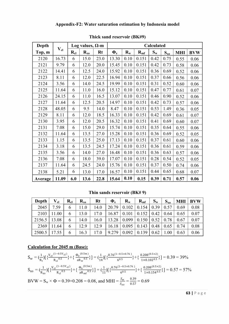
63 | P a g e
Appendix-F2: Water saturation estimation by Indonesia model
Thick sand reservoir (BK#9)
Depth Vcl
Log values, Ω-m Calculated Top, m Rcl Rxo Rt Φe Rw Rmf Sw Sxo MHI BVW
2120 16.73 6 15.0 23.0 13.30 0.10 0.151 0.42 0.75 0.55 0.06 2121 9.79 6 12.0 20.0 15.45 0.10 0.151 0.42 0.73 0.58 0.06 2122 14.41 6 12.5 24.0 15.92 0.10 0.151 0.36 0.69 0.52 0.06 2123 8.11 6 12.0 22.5 16.94 0.10 0.151 0.37 0.66 0.56 0.06 2124 3.56 6 14.0 24.5 19.99 0.10 0.151 0.31 0.52 0.60 0.06 2125 11.64 6 11.0 16.0 15.12 0.10 0.151 0.47 0.77 0.61 0.07 2126 24.15 6 11.0 16.5 13.07 0.10 0.151 0.46 0.90 0.52 0.06 2127 11.64 6 12.5 20.5 14.97 0.10 0.151 0.42 0.73 0.57 0.06 2128 48.05 6 9.5 14.0 8.47 0.10 0.151 0.53 1.49 0.36 0.05 2129 8.11 6 12.0 18.5 16.33 0.10 0.151 0.42 0.69 0.61 0.07 2130 3.95 6 12.0 20.5 16.32 0.10 0.151 0.41 0.69 0.60 0.07 2131 7.08 6 15.0 29.0 15.74 0.10 0.151 0.35 0.64 0.55 0.06 2132 11.64 6 13.5 27.0 15.28 0.10 0.151 0.36 0.69 0.52 0.05 2133 1.15 6 13.5 25.0 17.13 0.10 0.151 0.37 0.61 0.60 0.06 2134 3.18 6 13.5 24.5 17.24 0.10 0.151 0.36 0.61 0.59 0.06 2135 3.56 6 14.0 27.0 16.48 0.10 0.151 0.36 0.63 0.57 0.06 2136 7.08 6 18.0 39.0 17.07 0.10 0.151 0.28 0.54 0.52 0.05 2137 11.64 6 24.5 24.0 15.76 0.10 0.151 0.37 0.50 0.74 0.06 2138 5.21 6 13.0 17.0 16.57 0.10 0.151 0.44 0.65 0.68 0.07
Average 11.09 6.0 13.6 22.8 15.64 0.10 0.15 0.39 0.71 0.57 0.06
Thin sands reservoir (BK# 9)
Depth Vcl Rcl Rxo Rt Φe Rw Rmf Sw Sxo MHI BVW 2045 7.59 6 11.0 14.0 20.79 0.102 0.154 0.39 0.57 0.69 0.08 2103 11.00 6 13.0 17.0 16.87 0.101 0.152 0.42 0.64 0.65 0.07
2156.5 13.08 6 14.0 16.0 13.28 0.099 0.150 0.52 0.78 0.67 0.07 2369 11.64 6 12.9 12.9 16.18 0.095 0.143 0.48 0.65 0.74 0.08
2500.5 17.55 6 16.3 17.0 9.279 0.092 0.139 0.62 1.00 0.63 0.06
Calculation for 2045 m (Base):
Sw = ( 1
Rt)[{Vcl
(1−0.5V cl )
Rcl0.5 }+{ Фe
(0.5m )
aR w0.5 }] = ( 1
14)[{0.76(1−0.5×0.76 )
60.5 }+{ 0.208(0.5×2)
1×0.1020.5 }] = 0.39 = 39%
Sxo = ( 1
Rxo)[{Vcl
(1−0.5V cl )
Rcl0.5 }+{ Фe
(0.5m )
aR mf0.5 }] = ( 1
11)[{0.76(1−0.5×0.76 )
60.5 }+{ 0.208(0.5×2)
1×0.154 0.5 }] = 0.57 = 57%
BVW = Sw × Ф = 0.39×0.208 = 0.08, and MHI = 𝑆𝑤𝑆𝑥𝑜
= 0.39
0.57 = 0.69

64 | P a g e
Appendix-F3: Water Saturation estimation by Simandoux model
Thick sand reservoir (BK#9)
Sand Zone TVD Resistivity, Ω-m Calculated (%) meter Rt Rsh Rw Vsh Φe Sw BVW
Sub-zone:1 2120 23.0 6.0 0.10 16.73 13.30 44.29 0.059 Sub-zone:2 2121 20.0 6.0 0.10 9.79 15.45 40.90 0.063 Sub-zone:3 2122 24.0 6.0 0.10 14.41 15.92 36.22 0.058 Sub-zone:4 2123 22.5 6.0 0.10 8.11 16.94 35.17 0.060 Sub-zone:5 2124 24.5 6.0 0.10 3.56 19.99 28.58 0.057 Sub-zone:6 2125 17.0 6.0 0.10 11.64 15.12 45.33 0.069 Sub-zone:7 2126 16.5 6.0 0.10 24.15 13.07 53.20 0.070 Sub-zone:8 2127 20.5 6.0 0.10 11.64 14.97 41.71 0.062 Sub-zone:9 2128 14.0 6.0 0.10 48.05 8.47 88.81 0.075 Sub-zone:10 2129 18.5 6.0 0.10 8.11 16.33 40.25 0.066 Sub-zone:11 2130 20.5 6.0 0.10 3.95 16.32 38.26 0.062 Sub-zone:12 2131 28.0 6.0 0.10 7.08 15.74 33.94 0.053 Sub-zone:13 2132 27.5 6.0 0.10 11.64 15.28 35.26 0.054 Sub-zone:14 2133 25.0 6.0 0.10 1.15 17.13 33.03 0.057 Sub-zone:15 2134 24.5 6.0 0.10 3.18 17.24 33.14 0.057 Sub-zone:16 2135 27.5 6.0 0.10 3.56 16.48 32.72 0.054 Sub-zone:17 2136 38.0 6.0 0.10 7.08 17.07 26.86 0.046 Sub-zone:18 2137 24.0 6.0 0.10 11.64 15.76 36.60 0.058 Sub-zone:19 2138 17.0 6.0 0.10 5.21 16.57 41.38 0.069
Average 0.10 11.09 15.64 40.30 0.063
Thin sands reservoir (BK#9)
TVD (meter) Resistivity, ohm-m Calculated (%) Top Base Rt Rsh Rw Vsh Φe Sw BVW 2042 2045 14.0 6.0 0.102 7.59 20.79 36.71 0.076 2100 2103 17.0 6.0 0.101 11.00 16.87 40.77 0.069
2150.5 2156.5 16.0 6.0 0.099 13.08 13.28 53.05 0.070 2363 2369 12.9 6.0 0.095 11.64 16.18 47.36 0.077
2498.5 2500.5 17.0 6.0 0.092 17.55 9.28 70.78 0.066
Calculation for 2042-2045 m interval:
Sw = (0.4Rw
Фe2 ) ×[ √{Vsh
2
Rsh2 + 5Фe
2
Rw Rt} - Vsh
Rsh ] = (0.4 ×0.102
0.2082 ) × [ √{0.0762
62 + 5 × 0.2082
0.102 × 14} – 0.076
6 ] = 36.71%
Gas saturation, Sg= 1-0.367=0.633 = 63.3% and BVW = Sw × Фe = 0.3673×0.208 = 0.076

65 | P a g e
Appendix-G: Log derived permeability from Wyllie-Rose method
Thick sand reservoir (BK#9)
Zone name Depth, TVD Porosity (%) Wylie-Rose Method (mD) Sub-zone:1 2120 13.30 36.94 Sub-zone:2 2121 15.45 71.55 Sub-zone:3 2122 15.92 81.61 Sub-zone:4 2123 16.94 107.34 Sub-zone:5 2124 19.99 221.99 Sub-zone:6 2125 15.12 65.06 Sub-zone:7 2126 13.07 34.21 Sub-zone:8 2127 14.97 62.16 Sub-zone:9 2128 8.47 5.07 Sub-zone:10 2129 16.33 91.20 Sub-zone:11 2130 16.32 91.07 Sub-zone:12 2131 15.74 77.63 Sub-zone:13 2132 15.28 68.15 Sub-zone:14 2133 17.13 112.50 Sub-zone:15 2134 17.24 115.81 Sub-zone:16 2135 16.48 94.92 Sub-zone:17 2136 17.07 110.94 Sub-zone:18 2137 15.76 78.05 Sub-zone:19 2138 16.57 97.40 Average
85.45
Thin sands reservoir (BK#9)
Thin sand, TVD (m) Porosity (Фe)
Wylie-Rose Method Top Base mD 2042 2045 20.7887 263.90 2100 2103 16.8687 105.23
2150.5 2156.5 13.2849 36.79 2363 2369 16.1828 87.67
2498.5 2500.5 9.27948 7.59
Calculation for 2042-2045 m depth interval:
Log derived permeability, KL = [ (CPERM × ФDPERM )
(SwirrEPERM )
2
] = (8581 × 0.2084.4 )
0.182
2
] = 263.90 mD

Presentation on
“FORMATION EVALUATION USING WIRELINE LOG DATA OF BAKHRABAD GAS FIELD”
Presented byMohammad Islam Miah
Project Supervisor: Prof. Dr. Mohammad Tamim
Date : 29 November, 2014

Presentation Outline
IntroductionObjectives
Location of the StudyMethodologyResults and Discussions
Uncertainty Conclusions
Recommendations

Introduction
Formation evaluation is the practice of determining both the physical and
chemical properties of rocks and the fluids they contain.
Wireline log data generally more used for formation evaluation (porosityassessment, water saturation and permeability estimation etc.)
Reservoir thickness, shale volume, Porosity and Fluid saturation areimportant parameters for reserve estimation,GIIP and reservoircharacterization.

Objectives ■ The main objective of the present study is formationevaluation of BK#9 that is to ascertain the followed parts:
Lithology identification
Detection of hydrocarbon bearing zone
Estimation of shale volume and reservoir thickness
Assessment of effective porosity
Determination of water saturation and
Estimation of log derived permeability

Previous Study of BK Field
This gas field is one of the onshore gas fields in Bangladesh
The presence of a potential gas bearing structure at Bakhrabad was first
recognized from the results of the gravity survey made by Pakistan
Petroleum Company in 1953 (Welldrill, 1989).
BK seismic mapping was prepared by (HHS) in 1986.
In 1990, IKM studied about “Gas Field Appraisal Project- Geological,
Geophysical, Petrophysical & Reservoir Engineering report of the BK Gas
Field” for BK-1 to BK-8.

Several reservoir engineering studies on BK field have been done
based on IKM findings (Z. Choudhury, 1999 and so on).
In October 2009, RPS Energy & Petrobangla studied “Petrophysical
Analysis of BK Gas Field” for BK 1 to BK 8.
After May 2013, BK#9 has been penetrated within this structure.
The formation evaluation of BK#9 has not been done yet. So this
new data can be used for future reservoir analysis.
Previous Study of BK Field-Cont’d

Location of Study Area
Figure 1: Location of BK Gas Field (Source: RDMD, Petrobangla)
Figure 2: Bakhrabad gas field (drilled) well locations (Sourse: BGFCL)
BK

Figure 3 Flow chart for log interpretation and formation evaluation
Log Interpretation Methodology

Lithology Identification
Shale or Clay zone: High concentration of radioactive minerals (K40, U & Th) High Gamma Ray reading/response
Sand or Shaly sand zone:
Low concentration of radioactive minerals (K, Th, U) Generally low GR reading/response

Figure 4: A typical example of resistivity log including lithology logs of hydrocarbon bearing thick sand (BK#9)

HC Bearing Zone Detection
Figure 5: Cross-over of major sand between compensated density and neutron logs

YVsh= [(Xlog-Xmin)/(Xmax-Xmin)] where Y= GR/K/Th
Xlog= GR/K/Th response in the formation of zone interest,
Xmin= GR/K/Th response in clean shale free formation and
Xmax= GR/K/Th response in clean shale zone over the entire log.
Larionov equation , Shale volume (Vsh) = 0.083(23.7 *Ish -1) for tertiary rocks
True resistivity method: Vsh=[{(Rcl/Rt)*(Rtmax-Rt)/ (Rtmax-Rcl)}^(1/1.5)]
Rcl = Resistivity of clay, Rtmax =maximum value from deep resistivityover the entire log andRt = from the zone of interest.
Vsh is the ratio of clay fraction to the bulk volume of reservoir rocks
Shale Content/Volume (Ish/Vsh)

Total porosity is defined as the ratio of pore space to the total volume of reservoir rock
The effective porosity (Фe) is the ratio of interconnected pore space volume to the total bulk volume of the rock.
Clay corrected Neutron porosity , Ф N,corr = ФN -V sh * Ф N,sh + Lithology correction (=0.04%).
Clay corrected bulk density, ρb,corr = ρb+Vcl(ρma- ρcl) Density porosity, ФD,corr = [(ρma- ρb,corr)/( ρma- ρf)] Neutron-Density combination Formula, Фe = [{(Ф N,corr) 2
+( Ф D,corr)2 }/2]0.5
Sonic porosity, ФS = [(ΔT log- ΔTma)/ (ΔTf- ΔTma)] where
Hilchie (1978) formula [3] for hydrocarbon effect: Фe = ФS × 0.7 for gas
Porosity Assessment

Geothermal gradient, Gg and Formation Water Resistivity, Rw
Gg = [{(BHT-Ts)/TD}×100]
Tf = [Ts+ (Gg/100)]
BHT=Bottom Hole Temperature in degree Fahrenheit, Tf= Formation Temperature Ts =the surface (ambient) temperature in degree Fahrenheit and TD is the Total Depth.
Rw = [(ФN-Dm
* Rt)/a] by Inverse Archie’s Formula
Wyllie and Rose method,KL = [CPERM*(Ф^DPERM /Sw,irr ^ EPERM]
2 in mD for dry gas

Sw is water fraction within the pore space of reservoir rock.
Indoonesia equation :For un-invaded zones, Sw = (1/Rt)[{Vcl (1-0.5Vcl) /( Rcl) 0.5}+{ Ф 0.5m/(aRw)0.5}]
Simandoux method for shaly sand reservoir :Sw = {(0.4Rw/ Фe2)}*[√ {(Vsh/Rsh)2 + (5Фe2)/ (Rw*Rt)} - Vsh/Rsh ] for sandstones where
Фe = clay corrected porosity, Rcl or Rsh = Clay resistivity from virgin zone Rt = True resistivity, m = Cementation exponent,a = Tortousity factor, n = Saturation exponent and Rsh = Shale resistivity.
Water Saturation (Sw) Estimation
Archie’s water saturation formula for clean sands (Archie, 1942):Sw =[(FRw/Rt)] (1/n) for un-invaded zone & Sxo=[{(F*Rxo)/Rmf}] (1/n) for
flushed zone where n is the saturation exponent, F =(a/Фm)

Results and Discussions

Log Availability & Quality
The quality of log data of the studied well is good except SP log In studied wells:
No depth shift has been found in the logs. No borehole caving ( Bite size=Caliper log, shows in sands interval) Mud cake developed (Bite size>Caliper log)
No environmental corrections were applied to the logs.
Log type Log Name
Borehole measurement log Caliper log with Bit size
Lithology logs Spectral and Natural Gamma Ray logSelf-Potential (SP) log
Resistivity Logs Array compensated true resistivity (Shallow and Deep Resistivity logs)
Porosity logs Spectral Density, Dual spaced Neutron logand BHC Sonic Array log

Lithology Identification
Lithology is mainly sand and shale where sand is the dominant fraction
GRmax & GRmin: 155API @2405m & 76 API@1912m
True resistivity: 12.9-22 ohm-m (Rt) for gas bearing sand
Average sand bulk density: about 2.37 gm/cc (Thick Sand-2120-2138m)
Average adj. shale density: about 2.39 gm/cc

Fig 6. Spectral and natural GR logs of thin sand-1 reservoir
Thin sand-1 (2042-2045 m

Fig. 7: Lithology and
Resistivity logs of BK#9 of thin sand-1
reservoir
Thin sand-1 (2042-2045 m
Thin sand-1 (2042-2045 m

Figure 8: Spectral density & Dual spaced neutron with GR logs

Figure 9:Boreholecompensatedsonic arraylog of BK#9
Thin sand-1 (2042-2045 m

Hydrocarbon Bearing Zone Detection& Reservoir Thickness
Hydrocarbon
bearing sand
zone:
6 zones
(2042 m to 2500.5
m TVD)

Shale Volume (Vsh)
Figure 10: Shale volume vs. formation depth of thick sand reservoir

Porosity Assessment
Table 5 Estimated porosity from neutron, density and sonic logs
Figure 11: Depth versus average porosity of thick sand reservoir
Rock matrix density(ρma)= 2.65& Fluid density= 1.0 gram/cc(fresh water based mud)

Geothermal Gradient, Gg and Formation Temperature, Tf
Gg: 3.948 0F/100 meter with of BKB#9
Tf of thick (major) sand depth interval: 163.71 to 164.42 0F.
It is found that this (2120-2138m TVD) well shows lower Gg
comparing with 5.91 0F/100m of G sand (IKM, 1991).
The Gg and Tf are varied with respect to depth of the formation.

Formation Water Resistivity, Rw
Sand type TVD, m Tf (deg F) Rw (ohm-m) Rmf (ohm-m)
Reference(Wet sand)
1964.5 - 0.104 0.157
Thin-1 2043.5 160.68 0.102 0.154Thin-2 2101.5 162.97 0.102 0.154
(Thick -1) 2129 164.06 0.100 0.151Thin-4 2153.5 165.03 0.099 0.150Thin-5 2366 173.42 0.095 0.143Thin-6 2499.5 178.69 0.092 0.139
Rw=0.2 @ 175 deg. F & Rws= 0.38@ 76 deg. F (IKM,1991)
Table Estimated Rw by Inverse Archie’s Formula

Estimation of Sw
Table 6 Estimated water saturation from different methodsFigure 12: Average water saturation of reservoir (thick sand-1)
The tortousity (a), saturation (n) andcementation exponent (m) value of 1, 2and 2.25 have been used for saturationestimation.

Log Derived Permeability, KL
Swirr of 18%, and CPERM= 8581 (RPS Energy, 2010)
Irreducible saturation exponent (EPERM) of 2.0, and porosity
constant (DPERM) of 4.4 (IKM, 1991)

Discussions Sand interval, sand and shaly sand appeared as alternating units
Vsh is 7.6 – 17.6 % from Gamma Ray log for 18m thick sand-1 From Gama Ray method, estimated shale volume is optimistic (than TRM and
others) and more reliable for calculating effective porosity for shaly sand gasreservoir
Neutron-density combination formula gives better results of porosity for shalysand (thick) gas reservoir of this field as 15.64%
For Sw estimation, Indonesian/Simdoux formula is more reliable for this well
Log derived permeability KL (7.59 to 263.90 mD) of this reservoirs

Comparison of Petrophysical Properties

Uncertainty Manual interpreted log readings may be slightly change
Matrix density and transit time can be changed for the heterogeneity of the
studied gas reservoir
Clean wet sand zones are uncommon in the studied well. As a result, the
estimation of corrected Rw may be wrong due to changing of cementation
exponent (m) and actual sub-surface formation temperature.
Exponents (a=1, m=2 and n=2) are critical in calculating porosity, formation
water resistivity and water saturation of flushed zones as well as un-invaded
zones.
Reservoir porosity and fluid saturation in sandstone may be changed
causes for grain size distribution and grain shapes, packing arrangement,
cementation and clay volume changes.

ConclusionsBased on the log interpretation and analyzed results:
The shales are laminated & gross reservoir thickness: 18m for thick sand
Estimated average Vsh is 7.59-17.55 % (GR Method)
porosity quality is good
Reservoir is productive (Sw=39.18-40.30 % (Thick sand)
Gas is also moveable within major and thin sands reservoir of this reservoirs
or formation.
KL from Wylie-Rose method has been estimated as 34-222 mD which is a
good permeability for sand reservoirs.
So the gas pools of this formation are potential for producing gas.

Recommendations To estimate the water saturation for a reservoir, the special or routine core
analysis is required.
The estimated reservoir thickness, porosity and hydrocarbon saturation can beused for future reserve estimation and reservoir properties analysis of thisformation.
To assess the quality of the gas reservoirs accurately, special logging toolssuch as NMR and BHI logs can be run with conventional wire line logs.
To date, no wells has been drilled in the flank of the structure that could tellthe extension and quality of the reservoir as well as its gas saturation,presence of fluid contact (GWC) and minimizes the uncertainty of estimationof hydrocarbon reserve.

AcknowledgementI would like to express my deepest gratitude to:
Professor Dr. Mohammad Tamim (Research Supervisor, PMRE depth, BUET)
Md. Abdus Sultan (GM-In charge, RDMD, Petrobangla)
Mr. Mijanur Rahman (GM-In charge, Geological Division, BAPEX)
Mr. Sheik Muktadir and Engr. Ashraf, BGFCL.
All Teachers, PMRE Dept., BUET.
THANKS TO ALL