formation pressures 05 - king petroleum service ltd 1. introduction 3 2. formation pore pressures 4...

Formation Pressures! 05An Overview!

Introduction to Well Engineering - 05 - Formation Pressures 1

1. Introduction 3

2. Formation Pore Pressures 4

3. Overburden Pressures 7

4. Abnormal Pressures 9

4.1 Origin of Subnormal Formation Pressures 12

4.2 Origin of Overpressured Formations 14

5. Drilling Problems: Abnormal Formation Pressures 18

6. Transition Zone 19

7. Prediction And Detection Of Abnormal Pressures 21

7.1 Predictive Techniques 21

7.2 Detection Techniques 21

7.2.1 Detection Based on Drilling Parameters 23

7.2.2 Drilling Mud Parameters 27

7.2.3 Drilled Cuttings 29

7.3 Con!rmation Techniques 32

8. Formation Fracture Gradient 33

8.1 Mechanism of Formation Breakdown 33

8.2 e Leak-Off Test, Limit Test and Formation Breakdown Test 34

8.2.1 Leak-Off Test Calculations 40

8.2.2 e Equivalent Circulating Density (ECD) of a $uid 42

8.2.3 MAASP 42

8.3 Calculating the Fracture Pressure of a Formation 42

8.4 Summary of Procedures 46

Contents


1. Introduction

The magnitude of the pressure in the pores of a formation, known as the formation pore pressure (or simply formation pressure), is an important consideration in many aspects of well planning and operations. It will influence the casing design and mud-weight selection, and will increase the chances of stuck pipe and well control problems. It is particularly important to be able to predict and detect high pressure zones, where there is the risk of a blow-out.

In addition to predicting the pore pressure in a formation it is also very important to be able to predict the pressure at which the rocks will fracture. These fractures can result in losses of large volumes of drilling fluids and, in the case of an influx from a shallow formation, fluids flowing along the fractures all the way to surface, potentially causing a blowout.

When the pore pressure and fracture pressure for all of the formations to be penetrated have been predicted the well will be designed, and the operation conducted, such that the pressures in the borehole neither exceed the fracture pressure, nor fall below the pore pressure in the formations being drilled.


2. Formation Pore Pressures

During a period of erosion and sedimentation, grains of sediment are continuously building up on top of each other, generally in a water filled environment. As the thickness of the layer of sediment increases, the grains of the sediment are packed closer together, and some of the water is expelled from the pore spaces. However, if the pore throats through the sediment are interconnecting all the way to surface the pressure of the fluid at any depth in the sediment will be same as that which would be found in a simple column of fluid. The pressure in the fluid in the pores of the sediment will only be dependent on the density of the fluid in the pore space, and the depth of the pressure measurement (equal to the height of the column of liquid). It will be independent of the pore size or pore throat geometry. The pressure of the fluid in the pore space (the pore pressure) can be measured and plotted against depth as shown in Figure 1. This type of diagram is known as a P-Z diagram.

Figure 1 - P-Z Diagram representing pore pressures

The pressure in the formations to be drilled is often expressed in terms of a pressure gradient. This gradient is derived from a line passing through a particular formation pore pressure, and a datum point at surface, and is known as the pore pressure gradient. The reasons for this will become apparent subsequently. The datum which is generally used during drilling operations is the drill floor elevation, but a more general datum level, used almost universally, is Mean Sea Level (MSL). When the pore throats through the sediment are interconnecting, the pressure of the fluid at any depth in the sediment will be same as that which would be found in a simple column of fluid, and therefore the pore pressure gradient is a straight line as shown in Figure 1. The gradient of the line is a representation of the density of the fluid. Hence the density of the fluid in the pore space is often expressed in units of psi/ft.

Depth, ft.

OperationOperation

Pore PressureGeological

Section

Pressure, psi

Pore Pressure Profile

Pore Pressure Gradient, psi/ft

Pressure Gauge


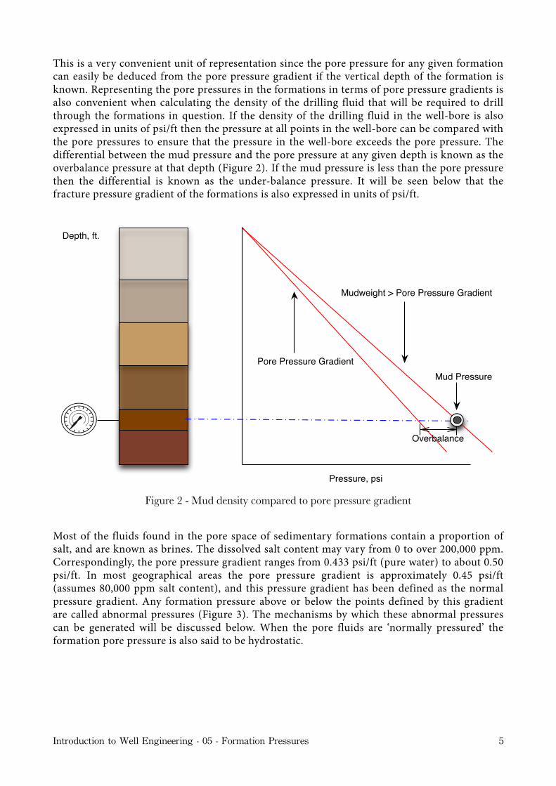
This is a very convenient unit of representation since the pore pressure for any given formation can easily be deduced from the pore pressure gradient if the vertical depth of the formation is known. Representing the pore pressures in the formations in terms of pore pressure gradients is also convenient when calculating the density of the drilling fluid that will be required to drill through the formations in question. If the density of the drilling fluid in the well-bore is also expressed in units of psi/ft then the pressure at all points in the well-bore can be compared with the pore pressures to ensure that the pressure in the well-bore exceeds the pore pressure. The differential between the mud pressure and the pore pressure at any given depth is known as the overbalance pressure at that depth (Figure 2). If the mud pressure is less than the pore pressure then the differential is known as the under-balance pressure. It will be seen below that the fracture pressure gradient of the formations is also expressed in units of psi/ft.

Depth, ft.

OperationOperation

Pressure, psi

Pore Pressure Gradient

Mudweight > Pore Pressure Gradient

Mud Pressure

Overbalance

Figure 2 - Mud density compared to pore pressure gradient

Most of the fluids found in the pore space of sedimentary formations contain a proportion of salt, and are known as brines. The dissolved salt content may vary from 0 to over 200,000 ppm. Correspondingly, the pore pressure gradient ranges from 0.433 psi/ft (pure water) to about 0.50 psi/ft. In most geographical areas the pore pressure gradient is approximately 0.45 psi/ft (assumes 80,000 ppm salt content), and this pressure gradient has been defined as the normal pressure gradient. Any formation pressure above or below the points defined by this gradient are called abnormal pressures (Figure 3). The mechanisms by which these abnormal pressures can be generated will be discussed below. When the pore fluids are ‘normally pressured’ the formation pore pressure is also said to be hydrostatic.


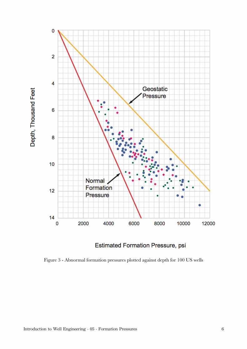
Figure 3 - Abnormal formation pressures plotted against depth for 100 US wells


3. Overburden Pressures

The pressures discussed above relate exclusively to the pressure in the pore space of the formations. It is however also important to be able to quantify the vertical stress at any depth, since this pressure will have a significant impact on the pressure at which the borehole will fracture when exposed to high pressures. The vertical pressure at any point in the earth is known as the overburden pressure, or geostatic pressure. The overburden gradient is derived from a cross plot of overburden pressure versus depth (Figure 4). The overburden pressure at any point is a function of the mass of rock and fluid above the point of interest. In order to calculate the overburden pressure at any point, the average density of the material (rock and fluids) above the point of interest must be determined.

Figure 4 - Pore pressure, fracture pressure, overburden pressures & gradients for a particular formation

The average density of the rock and fluid in the pore space is known as the bulk density of the rock:

or

Depth, ft.

OperationOperation

Pressure, psi

'Normal' Pore Pressure Gradient = 0.45 psi/ft

Geostatic Pressure (Overburden) Gradient

Fracture Pressure Gradient

ρb = ρ f x φ + ρm (1−φ)

ρb = ρm − (ρm − ρ f )φ


where;ρb = Bulk density of porous sedimentρm = Density of rock matrixρ f = Density of fluid in pore spaceφ = Porosity

Since the matrix material (rock type), porosity, and fluid content vary with depth, the bulk density will also vary with depth. The overburden pressure at any point is therefore the integral of the bulk density from surface down to the point of interest.

The specific gravity of the rock matrix may vary from 2.1 (sandstone) to 2.4 (limestone). Therefore, using an average of 2.3 and converting to units of psi/ft, it can be seen that the overburden pressure gradient exerted by a typical rock, with zero porosity would be:

This figure is normally rounded up to 1 psi/ft, and is commonly quoted as the maximum possible overburden pressure gradient, from which the maximum overburden pressure, at any depth, can be calculated. It is unlikely that the pore pressure could exceed the overburden pressure. However, it should be remembered that the overburden pressure may vary with depth, due to compaction and changing lithology, and so the gradient cannot be assumed to be constant.

2.3 x 0.433 psi/ft = 0.9959 psi/ft


ρbρmρ f

4. Abnormal Pressures

Pore pressures which are found to lie above or below the ‘normal’ pore pressure gradient line are called abnormal pore pressures (Figure 5 and 6). These formation pressures may be either Subnormal (i.e. less than 0.45 psi/ft), or Overpressured (i.e. greater than 0.45 psi/ft). The mechanisms which generate these abnormal pore pressures can be quite complex, and vary from region to region. However, the most common mechanism for generating overpressures is called ‘under compaction’, and can be best described by the under compaction model.

Figure 5 - Overpressure formation

Figure 6 - Under pressured (subnormal pressured) formation

Depth, ft.

OperationOperation

Pressure, psi


'Abnormal' Pressure Gradient > 0.465 psi/ft

Overpressured (Abnormally Pressured)

Formation

Overpressure

Depth, ft.

OperationOperation

Pressure, psi

'Abnormal' Pressure Gradient < 0.45 psi/ft

'Normal' Pressure Gradient > 0.465 psi/ft

Underpressured (Abnormally Pressured)

Formation

Underpressure


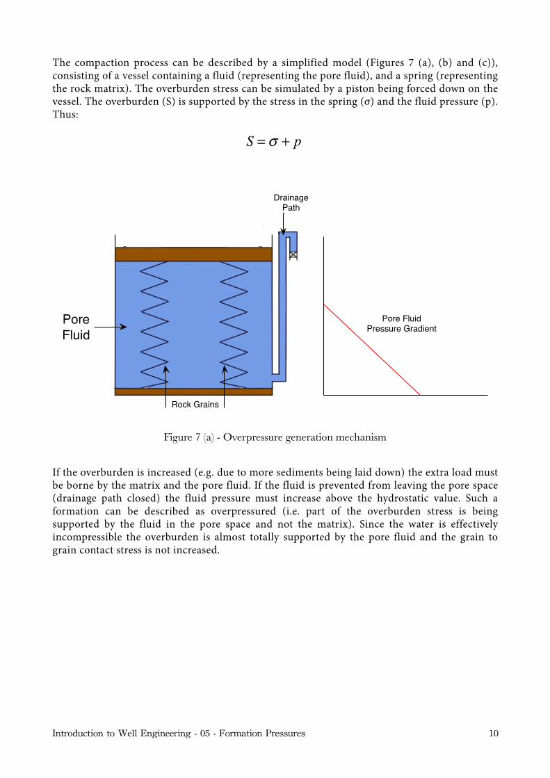
The compaction process can be described by a simplified model (Figures 7 (a), (b) and (c)), consisting of a vessel containing a fluid (representing the pore fluid), and a spring (representing the rock matrix). The overburden stress can be simulated by a piston being forced down on the vessel. The overburden (S) is supported by the stress in the spring (σ) and the fluid pressure (p). Thus:

Figure 7 (a) - Overpressure generation mechanism

If the overburden is increased (e.g. due to more sediments being laid down) the extra load must be borne by the matrix and the pore fluid. If the fluid is prevented from leaving the pore space (drainage path closed) the fluid pressure must increase above the hydrostatic value. Such a formation can be described as overpressured (i.e. part of the overburden stress is being supported by the fluid in the pore space and not the matrix). Since the water is effectively incompressible the overburden is almost totally supported by the pore fluid and the grain to grain contact stress is not increased.

S =σ + p

Pore Fluid

Pore FluidPressure Gradient

Rock Grains

DrainagePath


Figure 7(b) - Overpressure generation mechanism

In a formation where Th.e fluids are free to move (drainage path open), the increased load must be taken by the matrix, while the fluid pressure remains constant. Under such circumstances the pore pressure can be described as Normal, and is proportional to depth and fluid density.

Pore Fluid

Pore FluidPressure GradientRemains Constant

Rock Grains

Overburden

DrainagePath Open

Figure 7(c) - Overpressure generation mechanism

Pore Fluid Pore Fluid

Pressure Increases

Rock Grains

Overburden DrainagePath

Closed


In order for abnormal pressures to exist the pressure in the pores of a rock must be sealed in place i.e. the pores are not interconnecting. The seal prevents equalization of the pressures which occur within the geological sequence. The seal is formed by an impermeable barrier, generated from physical or chemical action. A physical seal may be formed by gravity faulting during deposition or the deposition of a fine grained material. The chemical seal may be due to Calcium Carbonate being deposited, thus restricting permeability. Another example might be chemical diagenesis during compaction of organic material. Both physical and chemical action may occur simultaneously to form a seal (e.g. gypsum-evaporite action).

4.1 Origin of Subnormal Formation Pressures

The major mechanisms by which subnormal (less than hydrostatic) pressures occur may be summarized as follows:

(a) Thermal Expansion

As sediments and pore fluids are buried the temperature rises. If the fluid is allowed to expand the density will decrease, and the pressure will reduce.

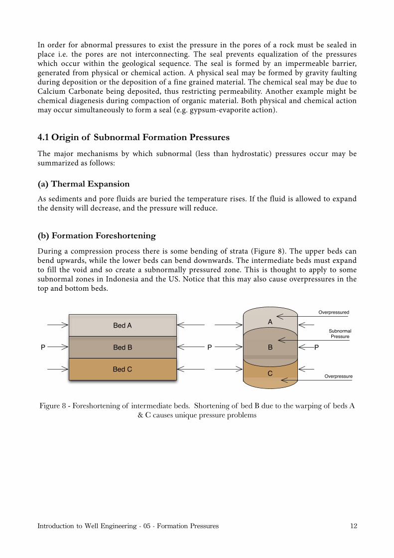
(b) Formation Foreshortening

During a compression process there is some bending of strata (Figure 8). The upper beds can bend upwards, while the lower beds can bend downwards. The intermediate beds must expand to fill the void and so create a subnormally pressured zone. This is thought to apply to some subnormal zones in Indonesia and the US. Notice that this may also cause overpressures in the top and bottom beds.

Figure 8 - Foreshortening of intermediate beds. Shortening of bed B due to the warping of beds A & C causes unique pressure problems

Bed A

Bed B

Bed C

P P

A

B

C

P

Overpressured

Subnormal Pressure

Overpressure


(c) Depletion

When hydrocarbons or water are produced from a competent formation in which no subsidence occurs, a subnormally pressured zone may result. This will be important when drilling development wells through a reservoir which has already been producing for some time. This is particularly relevant in some High Pressure High Temperature (HPHT) gas depletion drive reservoirs in the North Sea.

(d) Precipitation

In arid areas (e.g. Middle East) the water table may be located hundreds of feet below surface, thereby reducing the hydrostatic pressures.

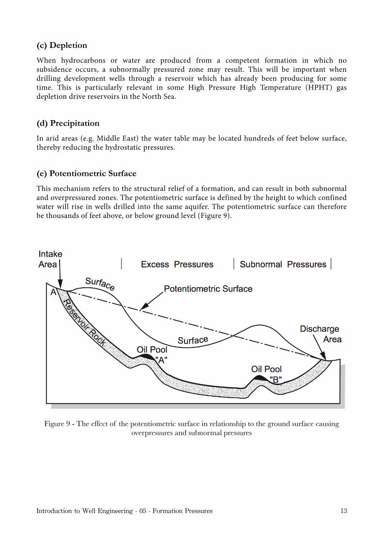
(e) Potentiometric Surface

This mechanism refers to the structural relief of a formation, and can result in both subnormal and overpressured zones. The potentiometric surface is defined by the height to which confined water will rise in wells drilled into the same aquifer. The potentiometric surface can therefore be thousands of feet above, or below ground level (Figure 9).

Figure 9 - The effect of the potentiometric surface in relationship to the ground surface causing overpressures and subnormal pressures


(f) Epeirogenic Movements

A change in elevation can cause abnormal pressures in formations open to the surface laterally, but otherwise sealed. If the outcrop is raised this will cause overpressures, if lowered it will cause subnormal pressures (Figure 10).

Figure 10 - Section through a sedimentary basin showing two potentiometric surfaces relating to the two reservoirs A and B

Pressure changes are seldom caused by changes in elevation alone since associated erosion and deposition are also significant. Loss or gain of water-saturated sediments is also important. The level of underpressuring is usually so slight it is not of any practical concern. By far the largest number of abnormal pressures reported have been overpressures, and not subnormal pressures.

4.2 Origin of Overpressured Formations

These are formations whose pore pressure is greater than that corresponding to the normal gradient of 0.45 psi/ft. As shown in Figure 11 these pressures can be plotted between the hydrostatic gradient, and the overburden gradient (1 psi/ft). The following examples of overpressures have been reported:

Gulf Coast 0.8 - 0.9 psi/

Iran 0.71 - 0.98 psi/

North Sea 0.5 - 0.9 psi/

Carpathian Basin 0.8 - 1.1 psi/


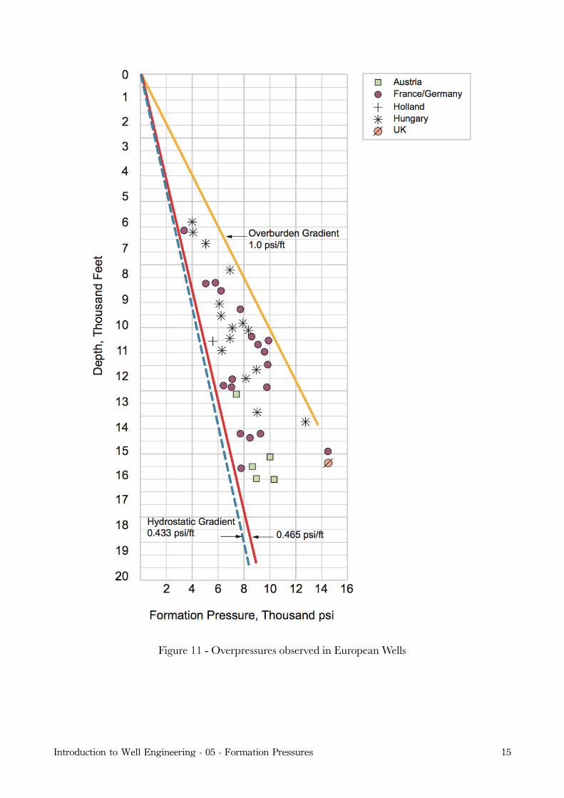
Figure 11 - Overpressures observed in European Wells


From the list it can be seen that overpressures occur worldwide. Some results from European fields are given in Figure 11. There are numerous mechanisms which cause such pressures to develop. Some, such as potentiometric surface, and formation foreshortening, have already been mentioned under subnormal pressures since both effects can occur as a result of these mechanisms. The other major mechanisms are summarized below:

(a) Incomplete Sediment Compaction

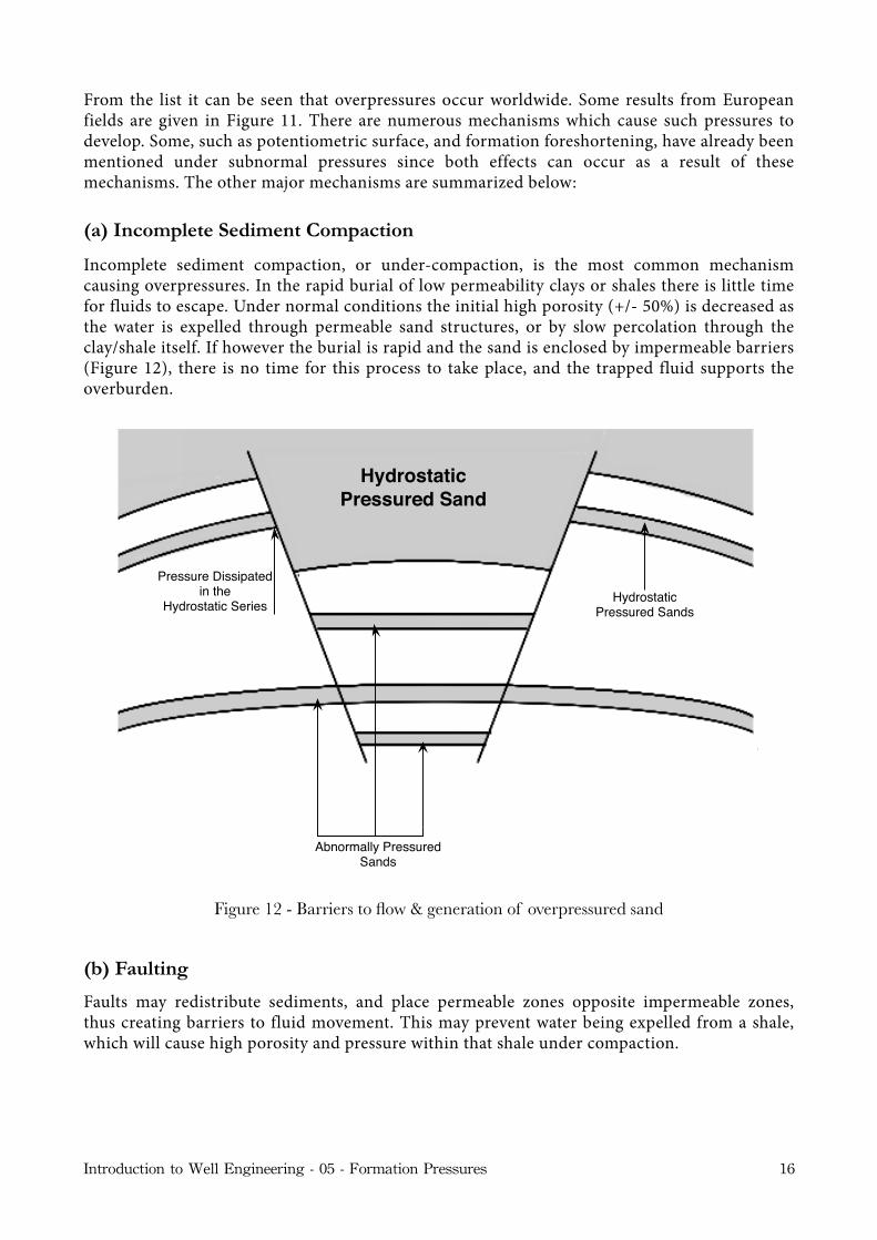
Incomplete sediment compaction, or under-compaction, is the most common mechanism causing overpressures. In the rapid burial of low permeability clays or shales there is little time for fluids to escape. Under normal conditions the initial high porosity (+/- 50%) is decreased as the water is expelled through permeable sand structures, or by slow percolation through the clay/shale itself. If however the burial is rapid and the sand is enclosed by impermeable barriers (Figure 12), there is no time for this process to take place, and the trapped fluid supports the overburden.

Figure 12 - Barriers to flow & generation of overpressured sand

(b) Faulting

Faults may redistribute sediments, and place permeable zones opposite impermeable zones, thus creating barriers to fluid movement. This may prevent water being expelled from a shale, which will cause high porosity and pressure within that shale under compaction.

Abnormally Pressured Sands

Pressure Dissipated in the

Hydrostatic Series Hydrostatic Pressured Sands

HydrostaticPressured Sand


(c) Phase Changes during Compaction

Minerals may change phase under increasing pressure, e.g. gypsum converts to anhydrite plus free water. It has been demonstrated that a phase change in gypsum will result in the release of water. The volume of water released is approximately 40% of the volume of the gypsum. If the water cannot escape then overpressures will be generated. Conversely, when anhydrite is hydrated at depth it will yield gypsum and result in a 40% increase in rock volume. The transformation of Montmorillonite to Illite also releases large amounts of water.

(d) Massive Rock Salt Deposition

Deposition of salt can occur over wide areas. Since salt is impermeable to fluids the underlying formations become overpressured. Abnormal pressures are frequently found in zones directly below a salt layer.

(e) Salt Diaperism

This is the upwards movement of a low density salt dome due to buoyancy which disturbs the normal layering of sediments, and produces pressure anomalies. The salt may also act as an impermeable seal to lateral dewatering of clays.

(f) Tectonic Compression

The lateral compression of sediments may result either in uplifting weathered sediments or, fracturing/faulting of stronger sediments. Thus formations normally compacted at depth can be raised to a higher level. If the original pressure is maintained the uplifted formation becomes overpressured.

(g) Repressuring from Deeper Levels

This is caused by the migration of fluid from a high to a low presssure zone at shallower depth. This may be due to faulting or from a poor casing/cement job. The unexpectedly high pressure could cause a kick, since no lithology change would be apparent. High pressures can occur in shallow sands if they are charged by gas from lower formations.

(h) Generation of Hydrocarbons

Shales which are deposited with a large content of organic material will produce gas as the organic material degrades under compaction. If it is not allowed to escape the gas will cause overpressures to develop. The organic by-products will also form salts which will be precipitated into the pore space, thus helping to reduce porosity and create a seal.


5. Drilling Problems: Abnormal Formation Pressures

When drilling through a formation sufficient hydrostatic mud pressure must be maintained to:

Prevent the borehole collapsing.

Prevent the in$ux of formation $uids.

To meet these 2 requirements the mud pressure is kept slightly higher than formation pressure. This is known as overbalance. If, however, the overbalance is too great this may lead to:

Reduced penetration rates (due to chip hold down effect).

Breakdown of formation (exceeding the fracture gradient) and subsequent lost circulation ($ow of mud into formation).

Excessive differential pressure causing stuck pipe.

The formation pressure will also influence the design of casing strings. If there is a zone of high pressure above a low pressure zone the same mud-weight cannot be used to drill through both formations, otherwise the lower zone may be fractured. The upper zone must be ‘cased off ’, allowing the mud-weight to be reduced for drilling the lower zone. A common problem is where the surface casing is set too high, so that when an overpressured zone is encountered and an influx is experienced, the influx cannot be circulated out with heavier mud without breaking down the upper zone. Each casing string should be set to the maximum depth allowed by the fracture gradient of the exposed formations. If this is not done an extra string of protective casing may be required. This will not only prove expensive, but will also reduce the well-bore diameter. This may have implications when the well is to be completed, since the production tubing size may have to be restricted.

Having considered some of these problems it should be clear that any abnormally pressured zone must be identified, and the drilling programme designed to accommodate it.


6. Transition Zone

It is clear from the descriptions of the ways in which overpressures are generated that the pore pressure profile in a region where overpressures exist will look something like the P-Z diagram shown in Figure 13. It can be seen that the pore pressures in the shallower formations are ‘normal’. That is that they correspond to a hydrostatic fluid gradient. There is then an increase in pressure with depth until the ‘overpressured’ formation is entered. The zone between the normally pressured zone and the overpressured zone is known as the transition zone.

The pressures in both the transition and overpressured zones are quite clearly above the hydrostatic pressure gradient line. The transition zone is therefore the seal or caprock on the overpressured formation. It is important to note that the transition zone shown in Figure 13 is representative of a thick shale sequence. This shale will have some low level of porosity and the fluids in the pore space can therefore be overpressured. However, the permeability of the shale is so low that the fluid in the shale, and in the overpressured zone below the shale, cannot flow through the shale, and is therefore effectively trapped. Hence the caprock of a reservoir is not necessarily a totally impermeable formation, but is generally simply a very low permeability formation.

If the seal is a thick shale, the increase in pressure will be gradual and there are techniques for detecting the increasing pore pressure. However, if the seal is a hard, crystalline rock (with no permeability at all) the transition will be abrupt, and it will not be possible to detect the increase in pore pressure across the seal.

When drilling in a region which is known to have overpressured zones the drilling crew will therefore be monitoring various drilling parameters, the mud, and the drilled cuttings in an attempt to detect this increase in pressure in the transition zone. It is the transition zone which provides the opportunity for the drilling crew to realise that they are entering an overpressured zone. The key to understanding this operation is to understand that although the pressure in the transition zone may be quite high, the fluid in the pore space cannot flow into the well-bore. When however the drill-bit enters the high permeability, overpressured zone below the transition zone, the fluids will flow into the well-bore. In some areas operating companies have adopted the policy of deliberately reducing the overbalance so as to detect the transition zone more easily, even if this means taking a kick.

It should be noted that the overpressures in a transition zone cannot result in an influx of fluid into the well since the seal has, by definition, an extremely low permeability. The overpressures must therefore be detected in some other way.


Figure 13 - Transition from normal pressures to overpressures


7. Prediction And Detection Of Abnormal Pressures

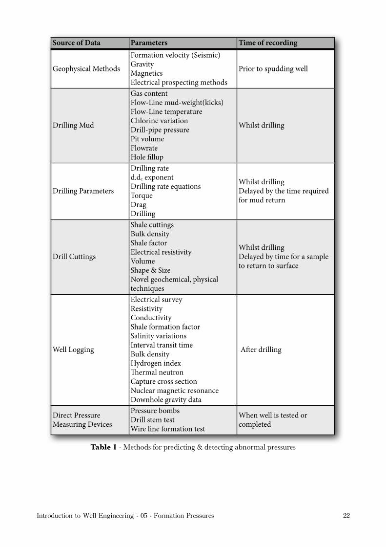
The techniques which are used to predict (before drilling), detect (whilst drilling) and confirm (after drilling) overpressures are summarised in Table 1.

7.1 Predictive Techniques

The predictive techniques are based on measurements that can be made at surface, such as geophysical measurements, or by analyzing data from wells that have been drilled in nearby locations (offset wells). Geophysical measurements are generally used to identify geological conditions which might indicate the potential for overpressures, such as salt domes which may have associated overpressured zones. Seismic data has been used successfully to identify transition zones, and fluid content such as the presence of gas. Offset well histories may contain information on mud-weights used, problems with stuck pipe, lost circulation or kicks. Any wireline logs or mud-logging information is also valuable when attempting to predict overpressures.

7.2 Detection Techniques

Detection techniques are used whilst drilling the well. They are basically used to detect an increase in pressure in the transition zone. They are based on three forms of data:

Drilling parameters - observing drilling parameters (e.g. ROP) and applying empirical equations to produce a term which is dependent on pore pressure.

Drilling mud - monitoring the effect of an overpressured zone on the mud (e.g. in temperature, in$ux of oil or gas).

Drilled cuttings - examining cuttings, trying to identify cuttings from the sealing zone.


Source of Data Parameters Time of recording

Geophysical Methods

Formation velocity (Seismic)GravityMagneticsElectrical prospecting methods

Prior to spudding well

Drilling Mud

Gas contentFlow-Line mud-weight(kicks)Flow-Line temperatureChlorine variationDrill-pipe pressurePit volumeFlowrateHole !llup

Whilst drilling

Drilling Parameters

Drilling rated.dc exponentDrilling rate equationsTorqueDragDrilling

Whilst drillingDelayed by the time required for mud return

Drill Cuttings

Shale cuttingsBulk densityShale factorElectrical resistivityVolumeShape & SizeNovel geochemical, physical techniques

Whilst drillingDelayed by time for a sample to return to surface

Well Logging

Electrical surveyResistivityConductivityShale formation factorSalinity variationsInterval transit timeBulk densityHydrogen indexermal neutronCapture cross sectionNuclear magnetic resonanceDownhole gravity data

Aer drilling

Direct Pressure Measuring Devices

Pressure bombsDrill stem testWire line formation test

When well is tested or completed

Table 1 - Methods for predicting & detecting abnormal pressures


7.2.1 Detection Based on Drilling Parameters

The theory behind using drilling parameters to detect overpressured zones is based on the fact that:

Compaction of formations increases with depth. ROP will therefore, all other things being constant, decrease with depth.

In the transition zone the rock will be more porous (less compacted) than that in a normally compacted formation, and this will result in an increase in ROP. Also, as drilling proceeds, the differential pressure between the mud hydrostatic and formation pore pressure in the transition zone will reduce, resulting in a much greater ROP.

The use of the ROP to detect transition and therefore overpressured zones is a simple concept, but difficult to apply in practice. This is due to the fact that many factors affect the ROP, apart from formation pressure (e.g. rotary speed and WOB). Since these other effects cannot be held constant, they must be considered so that a direct relationship between ROP and formation pressure can be established. This is achieved by applying empirical equations to produce a ‘normalised’ ROP, which can then be used as a detection tool.

(a) The ‘d’ exponent

The ‘d’ exponent technique for detection of overpressures is based on a normalised drilling rate equation developed by Bingham (1964). Bingham proposed the following generalised drilling rate equation:

where;R = Penetration rate (ft/hr)N = Rotary speed (rpm)W = WOB (lb)B = Bit diameter (in.)a = Matrix strength constantd = Formation drillabilitye = Rotary speed exponent

Jordan and Shirley (1966) re-organised this equation to be explicit in ‘d’. This equation was then simplified by assuming that the rock which was being drilled did not change (a = 1), and that the rotary speed exponent (e) was equal to one. The rotary speed exponent has been found experimentally to be very close to one. This removed the variables which were dependent on lithology and rotary speed. This means however that the resulting equation can only be applied to one type of lithology, and theoretically at a single rotary speed.

R = aN e WB

⎛⎝⎜

⎞⎠⎟d


The latter is not too restrictive since the value of e is generally close to 1 (one). On the basis of these assumptions, and accepting these limitations, the following equation was produced:

This equation is known as the ‘d-exponent’ equation. Since the values of R, N, W and B are either known, or can be measured at surface, the value of the d-exponent can be determined, and plotted against depth for the entire well. Values of ‘d’ can be found by using the nomograph in Figure 14. Notice that the value of the d-exponent varies inversely with the drilling rate. As the bit drills into an overpressured zone the compaction and differential pressure will decrease, the ROP will increase, and so the d-exponent should decrease. An overpressured zone will therefore be identified by plotting d-exponent against depth, and seeing where the d-exponent reduces (Figure 15).

Figure 14 - Nomogram for calculating ‘d’ exponent

d =log R

60N⎛⎝⎜

⎞⎠⎟

log 12W106B

⎛⎝⎜

⎞⎠⎟


30,000

It should be noted that this equation takes into account variations in the major drilling parameters, but for accurate results the following conditions should be maintained:

No abrupt changes in WOB or RPM should occur, i.e. keep WOB and RPM as constant as possible.

To reduce the dependence on lithology the equation should be applied over small depth increments only (plot every 10 ).

A good thick shale is required to establish a reliable ‘trend’ line.

It can be seen that the d-exponent equation takes no account of mud-weight. Since mud-weight determines the pressure on the bottom of the hole the greater the mud-weight the greater the chip hold-down effect, and therefore the lower the ROP. A modified d-exponent (dc) which accounts for variations in mud-weight has therefore been derived:

where;MWn = "Normal" mud weightMWa = Actual mud weight

The dc exponent trend gives a better definition of the transition (Figure 15).

dc = dMWn

MWa

⎛⎝⎜

⎞⎠⎟


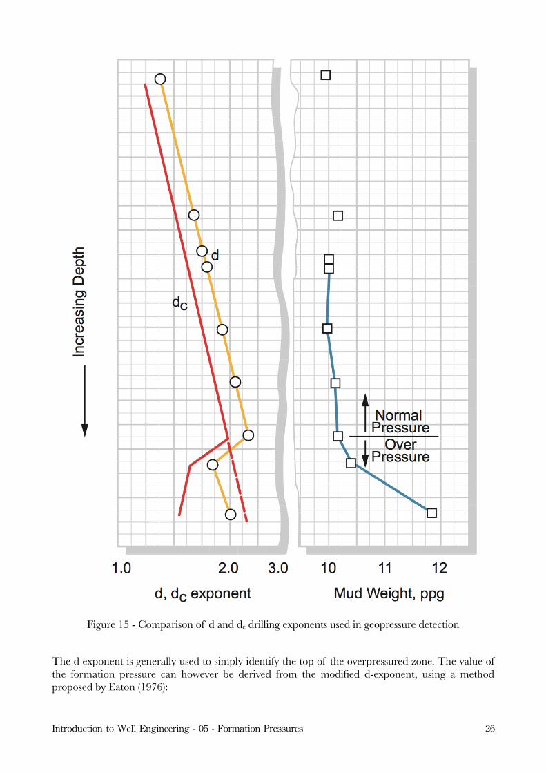
Figure 15 - Comparison of d and dc drilling exponents used in geopressure detection

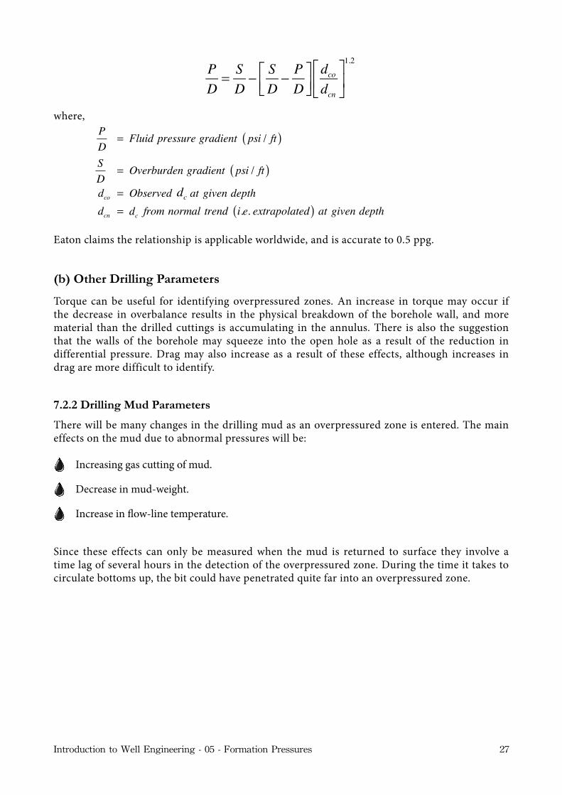
The d exponent is generally used to simply identify the top of the overpressured zone. The value of the formation pressure can however be derived from the modified d-exponent, using a method proposed by Eaton (1976):


where,PD

= Fluid pressure gradient psi / ft( )

SD

= Overburden gradient psi / ft( )dco = Observed dc at given depthdcn = dc from normal trend i.e. extrapolated( ) at given depth

Eaton claims the relationship is applicable worldwide, and is accurate to 0.5 ppg.

(b) Other Drilling Parameters

Torque can be useful for identifying overpressured zones. An increase in torque may occur if the decrease in overbalance results in the physical breakdown of the borehole wall, and more material than the drilled cuttings is accumulating in the annulus. There is also the suggestion that the walls of the borehole may squeeze into the open hole as a result of the reduction in differential pressure. Drag may also increase as a result of these effects, although increases in drag are more difficult to identify.

7.2.2 Drilling Mud Parameters

There will be many changes in the drilling mud as an overpressured zone is entered. The main effects on the mud due to abnormal pressures will be:

Increasing gas cutting of mud.

Decrease in mud-weight.

Increase in $ow-line temperature.

Since these effects can only be measured when the mud is returned to surface they involve a time lag of several hours in the detection of the overpressured zone. During the time it takes to circulate bottoms up, the bit could have penetrated quite far into an overpressured zone.

PD

= SD− S

D− PD

⎡⎣⎢

⎤⎦⎥dcodcn

⎡

⎣⎢

⎤

⎦⎥

1.2


dcdc

(a) Gas Cutting of Mud

Gas cutting of mud may happen in two ways:

From shale cuttings - if gas is present in the shale being drilled the gas may be released into the annulus from the cuttings.

Direct in!ux - this can happen if the overbalance is reduced too much.

or due to:

Swabbing when pulling back the drill-string at connections.

Continuous gas monitoring of the mud is done by the mud-logger using gas chromatography. A degasser is usually installed as part of the mud processing equipment so that entrained gas is not re-cycled downhole, or allowed to build up in the mud-pits.

(b) Mud-Weight

The mud-weight measured at the flow-line will be influenced by an influx of formation fluids. The presence of gas is readily identified due to the large decrease in density, but a water influx is more difficult to identify. Continuous measurement of mud-weight may be done by using a radioactive densometer.

(c) Flow-line Temperature

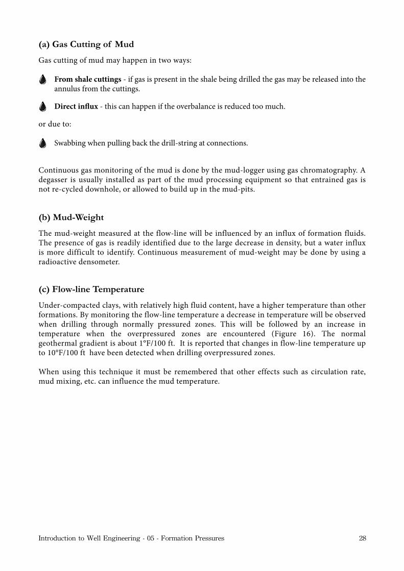
Under-compacted clays, with relatively high fluid content, have a higher temperature than other formations. By monitoring the flow-line temperature a decrease in temperature will be observed when drilling through normally pressured zones. This will be followed by an increase in temperature when the overpressured zones are encountered (Figure 16). The normal geothermal gradient is about 1°F/100 ft. It is reported that changes in flow-line temperature up to 10°F/100 ft have been detected when drilling overpressured zones.

When using this technique it must be remembered that other effects such as circulation rate, mud mixing, etc. can influence the mud temperature.


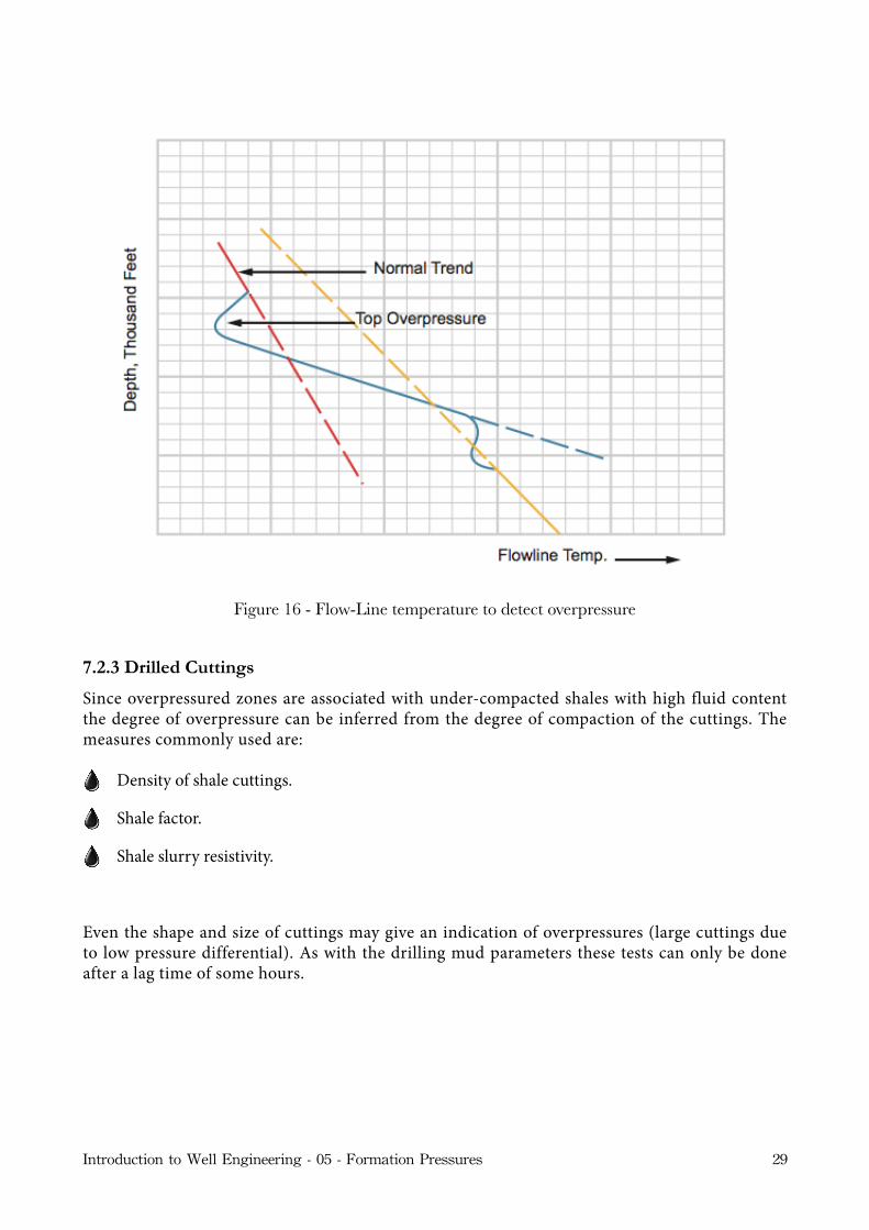
Figure 16 - Flow-Line temperature to detect overpressure

7.2.3 Drilled Cuttings

Since overpressured zones are associated with under-compacted shales with high fluid content the degree of overpressure can be inferred from the degree of compaction of the cuttings. The measures commonly used are:

Density of shale cuttings.

Shale factor.

Shale slurry resistivity.

Even the shape and size of cuttings may give an indication of overpressures (large cuttings due to low pressure differential). As with the drilling mud parameters these tests can only be done after a lag time of some hours.


(a) Density of Shale Cuttings

In normally pressured formations the compaction, and therefore the bulk density of shales, should increase uniformly with depth (given constant lithology). If the bulk density decreases, this may indicate an under-compacted zone which may be an overpressured zone. The bulk density of shale cuttings can be determined by using a mud balance. A sample of shale cuttings must first be washed and sieved (to remove cavings). These cuttings are then placed in the cup so that it balances at 8.3 ppg (equivalent to a full cup of water). At this point therefore:

where;ρs = Bulk density of shalerρw = Density of waterVs = Volume of shale cuttings Vt = Total volume of cup

The cup is then filled up to the top with water, and the reading is taken at the balance point (ρ). At this point:

Substituting for Vs from the first equation gives:

A number of such samples should be taken at each depth to check the density calculated as above and so improve the accuracy. The density at each depth can then be plotted (Figure 17).

ρsVs = ρwVt

ρVt = ρsVs + ρw (Vt −Vs )

ρs = ρw2

2ρw − ρ


ρs

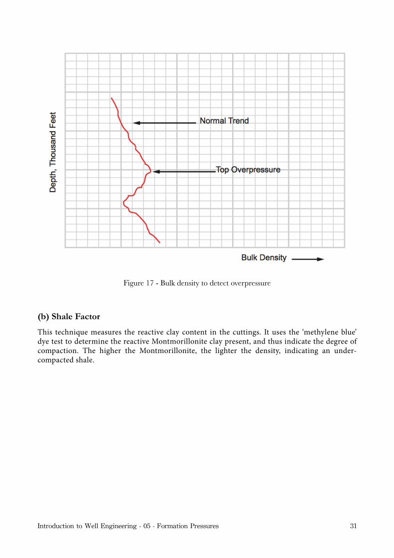
Figure 17 - Bulk density to detect overpressure

(b) Shale Factor

This technique measures the reactive clay content in the cuttings. It uses the ‘methylene blue’ dye test to determine the reactive Montmorillonite clay present, and thus indicate the degree of compaction. The higher the Montmorillonite, the lighter the density, indicating an under- compacted shale.


(c) Shale Slurry Resistivity

As compaction increases with depth, water is expelled and so conductivity is reduced. A plot of resistivity against depth should show a uniform increase in resistivity, unless an under compacted zone occurs, where the resistivity will reduce. To measure the resistivity of shale cuttings a known quantity of dried shale is mixed with a known volume of distilled water. The resistivity can then be measured and plotted (Figure 18).

Figure 18 - Resistivity to detect overpressure

7.3 Confirmation Techniques

After the hole has been successfully drilled certain electric wireline logs, and pressure surveys, may be run to confirm the presence of overpressures. The logs which are particularly sensitive to under-compaction are: the sonic, density and neutron logs. If an overpressured sand interval has been penetrated then the pressure in the sand can be measured directly with a repeat formation tester, or by conducting a well test.


8. Formation Fracture Gradient

When planning the well, both the formation pore pressure, and the formation fracture pressure, for all of the formations to be penetrated must be estimated (Figure 19). Well operations can then be designed such that the pressures in the borehole will always lie between the formation pore pressure, and the fracture pressure. If the pressure in the borehole falls below the pore pressure then an influx of formation fluids into the well-bore may occur. If the pressure in the borehole exceeds the fracture pressure then the formations will fracture, and losses of drilling fluid will occur.

Depth, ft.

OperationOperation

Pressure, psi


Geostatic Pressure (Overburden) Gradient

Fracture Pressure Gradient

Figure 19 - Pore pressure, fracture pressure and overburden pressures and gradients for a particular formation

8.1 Mechanism of Formation Breakdown

The stress within a rock can be resolved into three principal stresses (Figure 20). A formation will fracture when the pressure in the borehole exceeds the least of the stresses within the rock structure. Normally, these fractures will propagate in a direction perpendicular to the least principal stress (Figure 20). The direction of the least principal stress in any particular region can be predicted by investigating the fault activity in the area (Figure 21).

To initiate a fracture in the wall of the borehole, the pressure in the borehole must be greater than the least principal stress in the formation. To propagate the fracture the pressure must be maintained at a level greater than the least principal stress.


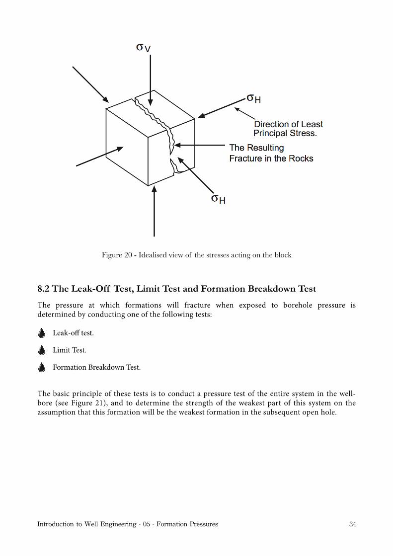
Figure 20 - Idealised view of the stresses acting on the block

8.2 The Leak-Off Test, Limit Test and Formation Breakdown Test

The pressure at which formations will fracture when exposed to borehole pressure is determined by conducting one of the following tests:

Leak-off test.

Limit Test.

Formation Breakdown Test.

The basic principle of these tests is to conduct a pressure test of the entire system in the well-bore (see Figure 21), and to determine the strength of the weakest part of this system on the assumption that this formation will be the weakest formation in the subsequent open hole.


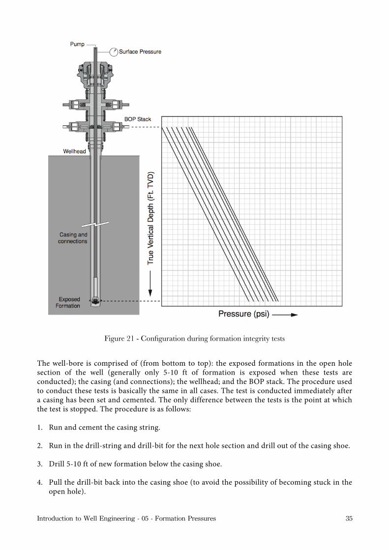
Figure 21 - Configuration during formation integrity tests

The well-bore is comprised of (from bottom to top): the exposed formations in the open hole section of the well (generally only 5-10 ft of formation is exposed when these tests are conducted); the casing (and connections); the wellhead; and the BOP stack. The procedure used to conduct these tests is basically the same in all cases. The test is conducted immediately after a casing has been set and cemented. The only difference between the tests is the point at which the test is stopped. The procedure is as follows:

1. Run and cement the casing string.

2. Run in the drill-string and drill-bit for the next hole section and drill out of the casing shoe.

3. Drill 5-10 ft of new formation below the casing shoe.

4. Pull the drill-bit back into the casing shoe (to avoid the possibility of becoming stuck in the open hole).


5. Close the BOP’s (generally the pipe ram) at surface.

6. Apply pressure to the well by pumping a small amount of mud (generally ½ bbl) into the well at surface. Stop pumping and record the pressure in the well. Pump a second, equal amount of mud into the well, and record the pressure at surface. Continue this operation, stopping after each increment in volume, and recording the corresponding pressure at surface. Plot the volume of mud pumped and the corresponding pressure at each increment in volume (Figure 22).

(Note: the graph shown in Figure 21 represents the pressure all along the well-bore at each increment. This shows that the pressure at the formation at leak-off is the sum of the pressure at surface plus the hydrostatic pressure of the mud).

7. When the test is complete, bleed off the pressure at surface, open the BOP rams and drill ahead.

It is assumed in these tests that the weakest part of the well-bore is the formations which are exposed just below the casing shoe. It can be seen in Figure 21, that when these tests are conducted, the pressure at surface, and throughout the well-bore, initially increases linearly with respect to pressure. At some pressure the exposed formations start to fracture, and the pressure no longer increases linearly for each increment in the volume of mud pumped into the well (see point A in Figure 22). If the test is conducted until the formations fracture completely (see point B in Figure 22) the pressure at surface will often drop dramatically, in a similar manner to that shown in Figure 22.

Figure 22 - Behaviour of a ductile rock


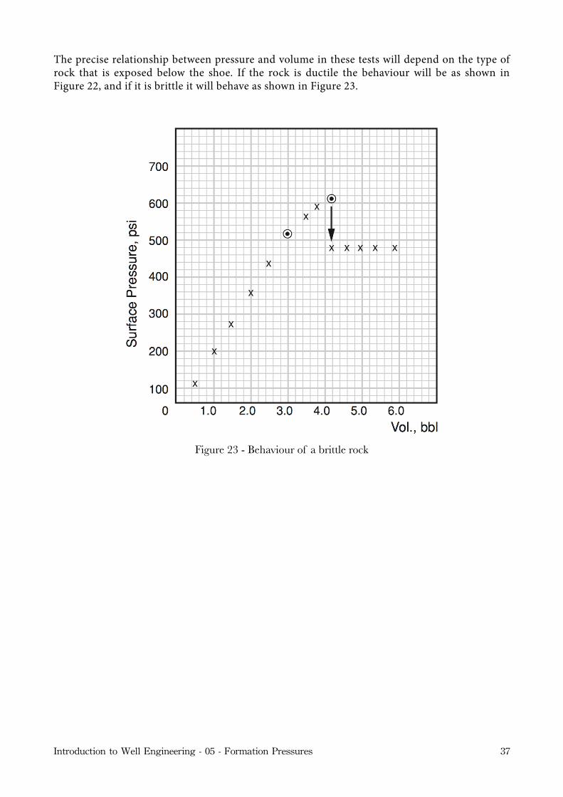
The precise relationship between pressure and volume in these tests will depend on the type of rock that is exposed below the shoe. If the rock is ductile the behaviour will be as shown in Figure 22, and if it is brittle it will behave as shown in Figure 23.

Figure 23 - Behaviour of a brittle rock


The ‘leak-off test’ is used to determine the pressure at which the rock in the open hole section of the well just starts to break down (or ‘leak-off ’). In this type of test the operation is terminated when the pressure no longer continues to increase linearly as the mud is pumped into the well (See Figure 24). In practice the pressure and volume pumped is plotted in real time, as the fluid is pumped into the well. When it is seen that the pressure no longer increases linearly with an increase in volume pumped (Point C) it is assumed that the formation is starting to breakdown. When this happens a second, smaller amount of mud (generally ¼ bbl) is pumped into the well just to check that the deviation from the line is not simply an error (Point D). If it is confirmed that the formation has started to ‘leak-off ’ then the test is stopped.

Figure 24 - P-V behaviour during a leak-off test


The ‘Limit Test’ is used to determine whether the rock in the open hole section of the well will withstand a specific, predetermined pressure. This pressure represents the maximum pressure that the formation will be exposed to whilst drilling the next well-bore section. The pressure to volume relationship during this test is shown in Figure 25. This test is effectively a limited version of the leak-off test.

Figure 25 - P-V behaviour in a limit test


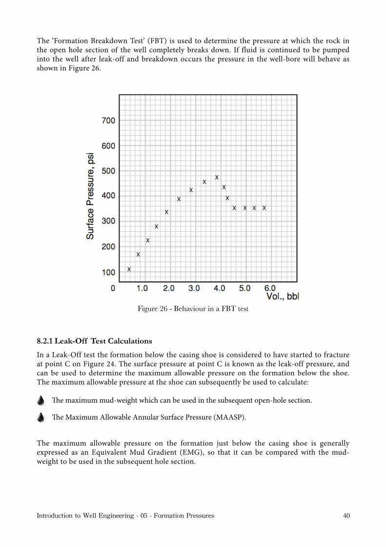
The ‘Formation Breakdown Test’ (FBT) is used to determine the pressure at which the rock in the open hole section of the well completely breaks down. If fluid is continued to be pumped into the well after leak-off and breakdown occurs the pressure in the well-bore will behave as shown in Figure 26.

Figure 26 - Behaviour in a FBT test

8.2.1 Leak-Off Test Calculations

In a Leak-Off test the formation below the casing shoe is considered to have started to fracture at point C on Figure 24. The surface pressure at point C is known as the leak-off pressure, and can be used to determine the maximum allowable pressure on the formation below the shoe. The maximum allowable pressure at the shoe can subsequently be used to calculate:

e maximum mud-weight which can be used in the subsequent open-hole section.

e Maximum Allowable Annular Surface Pressure (MAASP).

The maximum allowable pressure on the formation just below the casing shoe is generally expressed as an Equivalent Mud Gradient (EMG), so that it can be compared with the mud-weight to be used in the subsequent hole section.


Given the pressure at surface when leak-off occurs (point C in Figure 24) just below the casing shoe, the maximum mud-weight that can be used at that depth, and below, can be calculated from:

Usually a safety factor of 0.5 ppg (0.026 psi/ft) is subtracted from the allowable mud-weight.

It should be noted that the leak-off test is usually done just after drilling out of the casing shoe, but when drilling the next hole section other, weaker formations may be encountered.

Example:

While performing a leak-off test the surface pressure at leak-off was 940 psi. The casing shoe was at a true vertical depth of 5010 ft and a mud-weight of 10.2 ppg was used to conduct the test.

The Maximum bottom hole pressure during the leak-off test can be calculated from:

Hydrostatic pressure of column of mud + leak-off pressure at surface;

=3597 psi

The maximum allowable mud-weight at this depth is therefore:

= 3597 psi5010 ft

= 0.718 psi/ft = 13.8 ppg

Allowing a safety factor of 0.5 ppg, the maximum allowable mud-weight:

13.8 − 0.5 = 13.3 ppg

Maximum Mud −weight (psi / ft)

= Pressure at the shoe when Leak − off occursTrue Vertical Depth of the shoe

= Pressure at the surface and hydrostatic pressure of mud in wellTrue Vertical Depth of the shoe

= (0.052 x 10.2 x 5010) + 940


Maximum Mud weight (psi / ft)

8.2.2 The Equivalent Circulating Density (ECD) of a fluid

It is clear from all of the preceding discussion that the pressure at the bottom of the borehole must be accurately determined if the leak-off, or fracture pressure, of the formation is not to be exceeded. When the drilling fluid is circulating through the drill-string, the borehole pressure at the bottom of the annulus will be greater than the hydrostatic pressure of the mud. The extra pressure is due to the frictional pressure required to pump the fluid up the annulus. This frictional pressure must be added to the pressure due to the hydrostatic pressure from the column of mud, to get a true representation of the pressure acting against the formation a the bottom of the well. An Equivalent Circulating Density (ECD) can then be calculated from the sum of the hydrostatic and frictional pressure, divided by the true vertical depth of the well. The ECD for a system can be calculated from:

where;

ECD = Effective circulating density ppg( )MW = Mud weight ppg( )Pd = Annulus frictional pressure drop at a given circulation rate psi( ) D = Depth ft( )

The ECD of the fluid should be continuously monitored to ensure that the pressure at the formation below the shoe, due to the ECD of the fluid and system, does not exceed the leak-off test pressure.

8.2.3 MAASP

The Maximum Allowable Annular Surface Pressure (MAASP) when drilling ahead is the maximum closed in (not circulating) pressure that can be applied to the annulus (drill-pipe x BOP) at surface before the formation just below the casing shoe will start to fracture (leak-off). The MAASP can be determined from the following equation:

MAASP = Maximum allowable pressure at the formation just below the shoe minus the Hydrostatic Pressure of mud at the formation just below the shoe.

8.3 Calculating the Fracture Pressure of a Formation

The leak-off test pressure described above can only be determined after the formations to be considered have been penetrated. It is however necessary, in order to ensure a safe operation and to optimise the design of the well, to have an estimate of the fracture pressure of the formations to be drilled before the drilling operation has been commenced. In practice the fracture pressure of the formations are estimated from leak-off tests on nearby (offset) wells.

ECD = MW + Pd0.052 x D


Many attempts have been made to predict fracture pressures. If the conservative assumption that the formation is already fractured is made then, the equations used to calculate the fracture pressure of the formations are simplified significantly. The fracture pressure of a well drilled through a normally pressured formation can be determined from the following equations:

Vertical well and σ 2 =σ 3

Vertical well and σ 2 >σ 3

Deviated well and σ 2 =σ 3

Deviated well in the direction of σ 2 and σ 2 >σ 3

where;

FBP = Formation Breakdown Pressuresσ 1 = Overburden Stress psi( )σ 2 = Horizontal stress psi( )σ 3 = Horizontal stress psi( )Po = Pore Pressure psi( )θ z = Hole Deviation

Eaton proposed the following equation for fracture gradients:

FBP = 2σ 3 − Po

FBP = 3σ 3 −σ 2 − Po

FBP = 2σ 3 − (σ 1 −σ 3)sin2θ z − Po

FBP = 3σ 3 −σ 2 − (σ 1 −σ 3)sin2θ z − Po

Gf = Go −Gp⎡⎣ ⎤⎦v1− v⎡⎣⎢

⎤⎦⎥+Gp


where;

Gf = Fracture gradient psi / ft( )Go = Overburden gradient psi / ft( )Gp = Pore pressure gradient observed or predicted( ) psi / ft( )v = Poisson’s ratio

Poisson’s ratio is a rock property that describes the behaviour of rock stresses (σl) in one direction (least principal stress) when pressure (σp) is applied in another direction (principal stress):

Laboratory tests on unconsolidated rock have shown that generally:

Field tests however show that v may range from 0.25 to 0.5 at which point the rock becomes plastic (stresses equal in all directions). Poisson’s ratio varies with depth and degree of compaction (Figure 27).

σ 1

σ p

= v1− v

σ 1

σ p

= 13


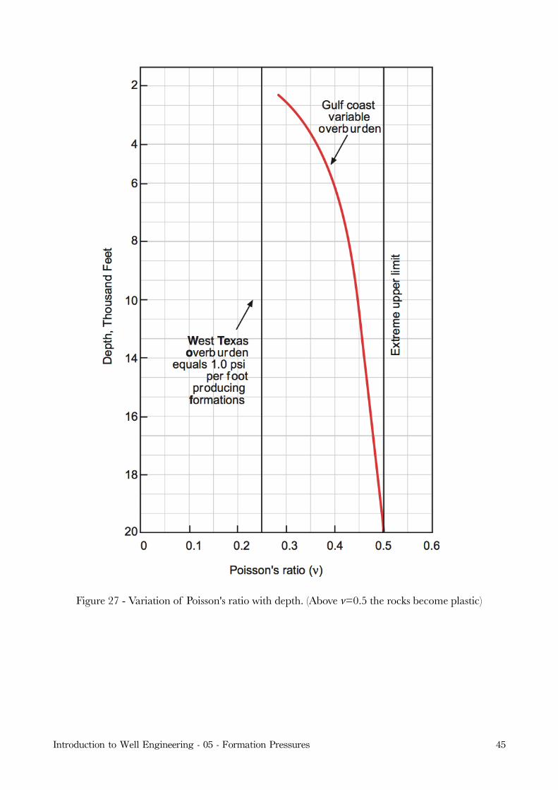
Figure 27 - Variation of Poisson's ratio with depth. (Above v=0.5 the rocks become plastic)


Matthews and Kelly proposed the following method for determination of fracture pressures in sedimentary rocks:

where;

Gf = Fracture gradient psi / ft( )Gp = Pore pressure gradient psi / ftKi = Matrix stress coefficientsσ = Matrix stress psi( )D = Depth of interest ft( )

The matrix stress (σ) can be calculated as the difference between overburden pressure, S, and pore pressure, P; i.e.

The coefficient Ki relates the actual matrix stress to the ‘normal’ matrix stress and can be obtained from charts.

8.4 Summary of Procedures

When planning a well the formation pore pressures, and fracture pressures, can be predicted from the following procedure:

1. Analyse and plot log data, or d-exponent data, from an offset (nearby) well.

2. Draw in the normal trend line, and extrapolate below the transition zone.

3. Calculate a typical overburden gradient using density logs from offset wells.

4. Calculate formation pore pressure gradients from equations (e.g. Eaton).

5. Use known formation and fracture gradients, and overburden data, to calculate a typical Poisson’s ratio plot.

6. Calculate the fracture gradient at any depth.

Gf = Gp +σKi

D

σ = S − P


( psi / ft)

formation pressures 05 - king petroleum service ltd 1. introduction 3 2. formation pore pressures 4...

Documents