formcalc 8 user’s guide - f-theory · in a way well suited for further numerical or analytical...
TRANSCRIPT

FormCalc 8 User’s GuideFebruary 12, 2015 Thomas Hahn
Abstract: FormCalc is a Mathematica package which calculates
and simplifies tree-level and one-loop Feynman diagrams. It ac-
cepts diagrams generated with FeynArts 3 and returns the results
in a way well suited for further numerical or analytical evalua-
tion.
2
The dreadful legal stuff: FormCalc is free software, but is not in the public domain. Instead it is covered by the GNU library
general public license. In plain English this means:
1) We don’t promise that this software works. (But if you find any bugs, please let us know!)
2) You can use this software for whatever you want. You don’t have to pay us.
3) You may not pretend that you wrote this software. If you use it in a program, you must acknowledge somewhere in your
publication that you’ve used our code.
If you’re a lawyer, you will rejoice at the exact wording of the license at http://gnu.org/licenses/lgpl.html.
FormCalc is available from http://feynarts.de/formcalc.
FeynArts is available from http://feynarts.de.
FORM is available from http://nikhef.nl/~form.
LoopTools is available from http://feynarts.de/looptools.
If you make this software available to others please provide them with this manual, too. There exists a low-traffic mailing list
where updates will be announced. Contact [email protected] to be added to this list.
If you find any bugs, or want to make suggestions, or just write fan mail, address it to:
Thomas Hahn
Max-Planck-Institut fur Physik
(Werner-Heisenberg-Institut)
Fohringer Ring 6
D–80805 Munich, Germany
e-mail: [email protected]

CONTENTS 3
Contents
1 General Considerations 5
2 Installation 7
3 Generating the Diagrams 7
4 Algebraically Simplifying Diagrams 8
4.1 CalcFeynAmp . . . . . . . . . . . . . . . . . . . . . . . . . . . . . . . . . . . . . . 8
4.2 DeclareProcess . . . . . . . . . . . . . . . . . . . . . . . . . . . . . . . . . . . . 14
4.3 Clearing, Combining, Selecting . . . . . . . . . . . . . . . . . . . . . . . . . . . 16
4.4 Ingredients of Feynman amplitudes . . . . . . . . . . . . . . . . . . . . . . . . 18
4.5 Handling Abbreviations . . . . . . . . . . . . . . . . . . . . . . . . . . . . . . . 23
4.6 More Abbreviations . . . . . . . . . . . . . . . . . . . . . . . . . . . . . . . . . . 25
4.7 Resuming Previous Sessions . . . . . . . . . . . . . . . . . . . . . . . . . . . . . 27
4.8 Fermionic Matrix Elements . . . . . . . . . . . . . . . . . . . . . . . . . . . . . 28
4.9 Colour Matrix Elements . . . . . . . . . . . . . . . . . . . . . . . . . . . . . . . 31
4.10 Putting together the Squared Amplitude . . . . . . . . . . . . . . . . . . . . . . 33
4.11 Polarization Sums . . . . . . . . . . . . . . . . . . . . . . . . . . . . . . . . . . . 34
4.12 Analytic Unsquared Amplitudes . . . . . . . . . . . . . . . . . . . . . . . . . . 36
4.13 Checking Ultraviolet Finiteness . . . . . . . . . . . . . . . . . . . . . . . . . . . 37
4.14 Useful Functions . . . . . . . . . . . . . . . . . . . . . . . . . . . . . . . . . . . 38
5 Tools for the Numerical Evaluation 39
5.1 Generating code . . . . . . . . . . . . . . . . . . . . . . . . . . . . . . . . . . . . 41
5.2 Running the Generated Code . . . . . . . . . . . . . . . . . . . . . . . . . . . . 50
5.2.1 Process definition . . . . . . . . . . . . . . . . . . . . . . . . . . . . . . . 51
5.2.2 Building up phase space . . . . . . . . . . . . . . . . . . . . . . . . . . . 52
5.2.3 Variables . . . . . . . . . . . . . . . . . . . . . . . . . . . . . . . . . . . . 54
5.2.4 Cuts . . . . . . . . . . . . . . . . . . . . . . . . . . . . . . . . . . . . . . 54
5.2.5 Convolution . . . . . . . . . . . . . . . . . . . . . . . . . . . . . . . . . . 56
5.2.6 Integration parameters . . . . . . . . . . . . . . . . . . . . . . . . . . . . 56
5.2.7 Compiling and running the code . . . . . . . . . . . . . . . . . . . . . . 57

4 CONTENTS
5.2.8 Parallelization and Vectorization . . . . . . . . . . . . . . . . . . . . . . 58
5.2.9 Scans over parameter space . . . . . . . . . . . . . . . . . . . . . . . . . 60
5.2.10 Log files, Data files, and Resume . . . . . . . . . . . . . . . . . . . . . . 62
5.2.11 Shell scripts . . . . . . . . . . . . . . . . . . . . . . . . . . . . . . . . . . 63
5.3 The Mathematica Interface . . . . . . . . . . . . . . . . . . . . . . . . . . . . . . 64
5.3.1 Setting up the Interface . . . . . . . . . . . . . . . . . . . . . . . . . . . 64
5.3.2 The Interface Function in Mathematica . . . . . . . . . . . . . . . . . . 65
5.3.3 Return values, Storage of Data . . . . . . . . . . . . . . . . . . . . . . . 66
5.3.4 Using the Generated Mathematica Function . . . . . . . . . . . . . . . 68
5.4 Renormalization Constants . . . . . . . . . . . . . . . . . . . . . . . . . . . . . 69
5.4.1 Definition of renormalization constants . . . . . . . . . . . . . . . . . . 69
5.4.2 Calculation of renormalization constants . . . . . . . . . . . . . . . . . 71
5.5 Infrared Divergences and the Soft-photon Factor . . . . . . . . . . . . . . . . . 73
6 Post-processing of the Results 74
6.1 Reading the data files into Mathematica . . . . . . . . . . . . . . . . . . . . . . . 74
6.2 Special graphics functions for Parameter Scans . . . . . . . . . . . . . . . . . . 77
7 Low-level functions for code output 78
7.1 File handling, Type conversion . . . . . . . . . . . . . . . . . . . . . . . . . . . 78
7.2 Writing Expressions . . . . . . . . . . . . . . . . . . . . . . . . . . . . . . . . . . 79
7.3 Variable lists and Abbreviations . . . . . . . . . . . . . . . . . . . . . . . . . . . 83
7.4 Declarations . . . . . . . . . . . . . . . . . . . . . . . . . . . . . . . . . . . . . . 86
7.5 Compatibility Functions . . . . . . . . . . . . . . . . . . . . . . . . . . . . . . . 87
5
1 General Considerations
With the increasing accuracy of experimental data, one-loop calculations have in many cases
come to be regarded as the lowest approximation acceptable to publish the results in a re-
spected journal. FormCalc goes a big step towards automating these calculations.
FormCalc is a Mathematica package which calculates and simplifies tree-level and one-loop
Feynman diagrams. It accepts diagrams generated with FeynArts 3 [Ha00] and returns the
results in a way well suited for further numerical (or analytical) evaluation.
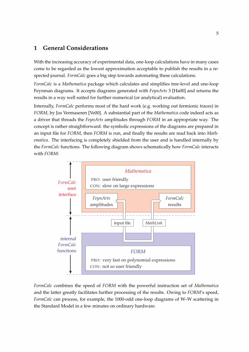
Internally, FormCalc performs most of the hard work (e.g. working out fermionic traces) in
FORM, by Jos Vermaseren [Ve00]. A substantial part of the Mathematica code indeed acts as
a driver that threads the FeynArts amplitudes through FORM in an appropriate way. The
concept is rather straightforward: the symbolic expressions of the diagrams are prepared in
an input file for FORM, then FORM is run, and finally the results are read back into Math-
ematica. The interfacing is completely shielded from the user and is handled internally by
the FormCalc functions. The following diagram shows schematically how FormCalc interacts
with FORM:
Mathematica
PRO: user friendly
CON: slow on large expressions
FeynArts
amplitudes
FormCalc
results
FORM
PRO: very fast on polynomial expressions
CON: not so user friendly
input file MathLink
FormCalc
user
interface
internal
FormCalc
functions
FormCalc combines the speed of FORM with the powerful instruction set of Mathematica
and the latter greatly facilitates further processing of the results. Owing to FORM’s speed,
FormCalc can process, for example, the 1000-odd one-loop diagrams of W–W scattering in
the Standard Model in a few minutes on ordinary hardware.

6 1 GENERAL CONSIDERATIONS
One important aspect of FormCalc is that it automatically gathers spinor chains, scalar prod-
ucts of vectors, and antisymmetric tensors contracted with vectors, and introduces abbre-
viations for them. In calculations with non-scalar external particles where such objects are
ubiquitous, code produced from the FormCalc output (say, in Fortran) can be significantly
shorter and faster than without the abbreviations.
FormCalc can work in D and 4 dimensions. In D dimensions it uses standard dimensional
regularization to treat ultraviolet divergences, in 4 dimensions it uses the method of con-
strained differential renormalization, which at the one-loop level is equivalent to dimen-
sional reduction. Details on these methods can be found in [Ha98].
A one-loop calculation generally includes three steps:
• Create the topologies
Diagram • Insert fields
generation • Apply the Feynman rules
• Paint the diagrams
FeynArts
↓• Contract indices
Algebraic • Calculate traces
simplification • Reduce tensor integrals
• Introduce abbreviations
FormCalc↓
• Convert Mathematica output
Numerical to Fortran/C code
evaluation • Supply a driver program
• Implementation of the integrals LoopTools
The automation of the calculation is fairly complete in FormCalc, i.e. FormCalc can eventually
produce a complete program to calculate the squared matrix element for a given process. The
only thing the user has to supply is a driver program which calls the generated subroutines.
The FormCalc distribution includes a directory of tools and sample programs which can be
modified and/or extended for a particular application. To demonstrate how a full process is
calculated, several non-trivial one-loop calculations in the electroweak Standard Model are
included in the FormCalc package.
It is nevertheless important to realize that the code is generated only at the very end of
the calculation (if at all), i.e. the calculation proceeds analytically as far as possible. At all
intermediate stages, the results are Mathematica expressions which are considerably easier to
modify than Fortran or C code.
7
2 Installation
To run FormCalc you need Mathematica 5 or above, a Fortran compiler, and gcc, the GNU C
compiler. FormCalc comes in a compressed tar archive FormCalc-n.m.tar.gz. To install it,
create a directory for FormCalc and unpack the archive there, e.g.
gunzip -c FormCalc-n.m.tar.gz | tar xvf -
cd FormCalc-n.m
./compile
The last line compiles the C programs that come with FormCalc. The compile script puts the
binaries in a system-dependent directory, e.g. Linux. A single FormCalc installation can thus
be NFS-mounted on different systems once compile has been run on each.
FormCalc by default invokes the executable form to run FORM. If FORM is installed under a
different name on your system, edit FormCalc.m and change the following line:
$FormCmd = "form"
3 Generating the Diagrams
FormCalc calculates diagrams generated by FeynArts Version 3 or above. Do not use the Feyn-
Arts function ToFA1Conventions to convert the output of CreateFeynAmp to the old conven-
tions of FeynArts 1.
FormCalc can be loaded together with FeynArts into one Mathematica session. The FeynArts
results thus need not be saved in a file before calculating them with FormCalc.
FormCalc can deal with any mixture of fully inserted diagrams and generic diagrams
with insertions. The former are produced by FeynArts if only one level is requested (via
InsertionLevel, AmplitudeLevel, or PickLevel; see the FeynArts manual). While both
types of input eventually produce the same results, it is important to understand that it
is the generic amplitude which is the most costly part to simplify, so using the latter type of
diagrams, where many insertions are derived from one generic amplitude, can significantly
speed up the calculation.
Usually it is also helpful to organize the diagrams into classes like self-energies, vertex cor-
rections and box corrections; it will also make the amplitudes easier to handle since it reduces
their size.
8 4 ALGEBRAICALLY SIMPLIFYING DIAGRAMS
4 Algebraically Simplifying Diagrams
4.1 CalcFeynAmp
FeynArts always produces purely symbolic amplitudes and refrains from simplifying them
in any way so as not to be restricted to a certain class of theories. Needless to say, the
resulting expressions cannot be used directly e.g. in a Fortran program, but must first be
simplified algebraically. The function for this is CalcFeynAmp.
CalcFeynAmp[a1, a2, . . . ] calculate the sum of amplitudes a1 + a2 + . . .
CalcFeynAmp performs the following simplifications:
• indices are contracted as far as possible,
• fermion traces are evaluated,
• open fermion chains are simplified using the Dirac equation,
• colour structures are simplified using the SU(N) algebra,
• the tensor reduction is performed,
• local terms are added∗,
• the results are partially factored,
• abbreviations are introduced.
The output of CreateFeynAmp can be fed directly into CalcFeynAmp. Technically, this means
that the arguments of CalcFeynAmp must be FeynAmpList objects. CalcFeynAmp is invoked
as
amps = CreateFeynAmp[...];
result = CalcFeynAmp[amps]
The results are returned in the form
Amp[in -> out][r1, r2, . . .]
∗In D dimensions, the divergent integrals are expanded in ε = (4 − D)/2 up to order ε0 and the 1ε poles are
subtracted. The 1ε poles give rise to local terms when multiplied with D’s from outside the integral (e.g. from
a gµµ). In 4 dimensions, local terms are added depending on the contractions of indices of the tensor integrals
according to the prescription of constrained differential renormalization [dA98].

4.1 CalcFeynAmp 9
The lists in and out in the head of Amp specify the the external particles to which the result
belongs. The presence of a particle’s mass in the header does not imply that the amplitudes
were calculated for on-shell particles.
The actual result is split into parts r1, r2, . . . , such that index sums (marked by SumOver)
always apply to the whole of each part. It is possible to extend this splitting also to powers
of coupling constants, such that part ri has a definite coupling order. To this end one needs
to wrap the coupling constants of interest in PowerOf, for example
CalcFeynAmp[amp /. g -> g PowerOf[g]]
The function PowerOf is there only to keep track of the coupling order and can be replaced
by 1 at the end of the calculation.
The full result – the sum of the parts – can trivially be recovered by applying Plus to the
outcome of CalcFeynAmp, i.e. Plus@@ CalcFeynAmp[amps].
CalcFeynAmp has the following options:
option default value
CalcLevel Automatic which level of the amplitude to select
(Automatic selects Particles level, if
available, otherwise Classes level)
Dimension D the space-time dimension in which the
calculation is performed (D, 4, or 0)
MomElim Automatic how to apply momentum conservation
DotExpand False whether to expand terms collected for
momentum elimination
NoCostly False whether to turn off potentially
time-consuming simplifications in
FORM
FermionChains Weyl how to treat external fermion chains
(Weyl, Chiral, or VA)
FermionOrder Automatic the preferred ordering of external
spinors in Dirac chains
Evanescent False whether to keep track of fermionic
operators across Fierz transformations
InsertionPolicy Default how the level insertions are processed

10 4 ALGEBRAICALLY SIMPLIFYING DIAGRAMS
option default value
SortDen True whether to sort the denominators of the
loop integrals
PaVeReduce False whether to reduce tensor to scalar
integrals
SimplifyQ2 True whether to simplify q2 in the numerator
OPP 100 the N in N-point function above which
OPP loop integrals are emitted
OPPQSlash False whether to introduce µ also on /q
Gamma5Test False whether to substitute
γ5 → γ5(1 + Gamma5Test(D − 4))
Gamma5ToEps False whether to substitute
γ5 → 14!εµνρσγ
µγνγργσ in fermion
traces
NoExpand sums containing any of the symbols in
the list are not expanded
NoBracket symbols not to be included in the
bracketing in FORM
MomRules extra rules for transforming momenta
PreFunction Identity a function applied to the amplitudes
before any simplification
PostFunction Identity a function applied to the amplitudes
after all simplifications
FileTag "amp" the middle part of the temporary FORM
file’s name
RetainFile False whether to retain the temporary FORM
input file
EditCode False whether to display the FORM code in
an editor before sending it to FORM
CalcLevel is used to select the desired level in the calculation. In general a diagram can have
both Classes and Particles insertions. The default value Automatic selects the deepest
level available, i.e. Particles level, if available, otherwise Classes level.
Dimension specifies the space-time dimension in which to perform the calculation. It can
take the values D and 4. This is a question of how UV-divergent expressions are treated.
The essential points of both methods are outlined in the following. For a more thorough

4.1 CalcFeynAmp 11
discussion see [Ha98].
• Dimension -> D corresponds to dimensional regularization [tH72]. Dimensionally
regularizing an expression involves actually two things: analytic continuation of the
momenta (and other four-vectors) in the number of dimensions, D, and an extension
to D dimensions of the Lorentz covariants (γµ, gµν, etc.). The second part is achieved
by treating the covariants as formal objects obeying certain algebraic relations. Prob-
lems only appear for identities that depend on the 4-dimensional nature of the objects
involved. In particular, the extension of γ5 to D dimensions is problematic. FormCalc
employs a naive scheme [Ch79] and works with an anticommuting γ5 in all dimen-
sions.
• Dimension -> 4 selects constrained differential renormalization (CDR) [dA98]. This
technique cures UV divergences by substituting badly-behaved expressions by deriva-
tives of well-behaved ones in coordinate space. The regularized coordinate-space ex-
pressions are then Fourier-transformed back to momentum space. CDR works com-
pletely in 4 dimensions. At one-loop level it has been shown [Ha98] to be equivalent
to regularization by dimensional reduction [Si79], which is a modified version of di-
mensional regularization: while the integration momenta are still D-dimensional as in
dimensional regularization, all other tensors and spinors are kept 4-dimensional. Al-
though the results are the same, it should be stressed that the conceptual approach in
CDR is quite different from dimensional reduction.
• Dimension -> 0 keeps the whole amplitude D-dimensional. No rational terms are
added and the D-dependency is expressed through Dminus4.
MomElim controls in which way momentum conservation is used to eliminate momenta.
False performs no elimination, an integer between 1 and the number of legs eliminates
the specified momentum in favour of the others, and Automatic tries all substitutions and
chooses the one resulting in the fewest terms.
DotExpand determines whether the terms collected for momentum elimination are expanded
again. This prevents kinematical invariants from appearing in the abbreviations but typi-
cally leads to poorer simplification of the amplitude.
NoCostly switches off simplifications in the FORM code which are typically fast but can
cause ‘endless’ computations on certain amplitudes.
FermionChains determines how fermion chains are returned. Weyl, the default, selects Weyl
chains. Chiral and VA select Dirac chains in the chiral (PL/PR) and vector/axial-vector
(1l/γ5) decomposition, respectively. Note that to fully evaluate amplitudes containing Dirac
chains, helicity matrix elements must be computed with HelicityME. For more details on
the conceptual treatment of external fermions in FormCalc, see [Ha02, Ha04a].

12 4 ALGEBRAICALLY SIMPLIFYING DIAGRAMS
FermionOrder specifies an ordering for the external spinors in Dirac chains, i.e. makes sense
only in combination with FermionChains -> Chiral or VA. Possible values are None, Fierz,
Automatic, Colour, or an explicit ordering, e.g. 2, 1, 4, 3 (corresponding to fermion
chains of the form 〈2| Γ |1〉 〈4| Γ ′ |3〉). None applies no reordering. Fierz applies the Fierz
identities [Ni05] twice, thus simplifying the chains but keeping the original order. Colour
applies the ordering of the external colour indices (after simplification) to the spinors.
Automatic chooses a lexicographical ordering (small numbers before large numbers).
The Evanescent option toggles whether fermionic operators are tracked across Fierz trans-
formations by emitting terms of the form Evanescent[original operator, Fierzed operator].
InsertionPolicy specifies how the level insertions are applied and can take the values
Begin, Default, or an integer. Begin applies the insertions at the beginning of the FORM
code (this ensures that all loop integrals are fully symmetrized). Default applies them af-
ter simplifying the generic amplitudes (this is fastest). An integer does the same, except
that insertions with a LeafCount larger than that integer are inserted only after the ampli-
tude comes back from FORM (this is a workaround for the rare cases where the FORM code
aborts due to very long insertions).
SortDen determines whether the denominators of loop integrals shall be sorted. This is
usually done to reduce the number of loop integrals appearing in an amplitude. Sorting
may be turned off for testing and in few cases may even lead to shorter amplitudes.
PaVeReduce governs the tensor reduction. False retains the one-loop tensor-coefficient func-
tions. Raw reduces them to scalar integrals but keeps the Gram determinants in the denomi-
nator in terms of dot products. True simplifies the Gram determinants using invariants.
SimplifyQ2 controls simplification of terms involving the integration momentum q squared.
If set to True, powers of q2 in the numerator are cancelled by a denominator, except for
OPP integrals, where conversely lower-N integrals are put on a common denominator with
higher-N integrals to reduce OPP calls, as in: N2/(D0D1) + N3/(D0D1D2) → (N2D2 +
N3)/(D0D1D2).
OPP specifies an integer N starting from which an N-point function is treated with OPP
methods. For example, OPP → 4 means that A, B, C functions are reduced with Passarino–
Veltman and D and up with OPP. A negative N indicates that the rational terms for the OPP
integrals shall be added analytically whereas otherwise their computation is left to the OPP
package (CutTools or Samurai).
The integration momentum q starts life as a D-dimensional object. In OPP, any q2 surviving
SimplifyQ2 is substituted by q2 − µ2, after which q is considered 4-dimensional. The di-
mensionful scale µ enables the OPP libraries to reconstruct the R2 rational terms. OPPQSlash
extends this treatment to the /q on external fermion chains, i.e. also substitutes /q → /q + iγ5µ,
where odd powers of µ are eventually set to zero.

4.1 CalcFeynAmp 13
Gamma5Test → True substitutes each γ5 by γ5(1 + Gamma5Test(D − 4)) and it can be tested
whether the final result depends on the variable Gamma5Test (which it shouldn’t).
Gamma5ToEps → True substitutes all γ5 in fermion traces by 14!εµνρσγ
µγνγργσ . This effec-
tively implements the ’t Hooft–Veltman–Breitenlohner–Maisonγ5-scheme. External fermion
chains are intentionally exempt since at least the Weyl formalism needs chiral chains. Take
care that due to the larger number of Lorentz indices the computation time may increase
significantly.
NoExpand prohibits the expansion of sums containing certain symbols. In certain cases, ex-
pressions can become unnecessarily bloated if all terms are fully expanded, as FORM always
does. For example, if gauge eigenstates are rotated into mass eigenstates, the couplings typ-
ically contain linear combinations of the form Ui1c1 + Ui2c2. It is not difficult to see that the
number of terms generated by the full expansion of such couplings can be considerable, in
particular if several of them appear in a diagram. NoExpand turns off the automatic expan-
sion, in this example one would select NoExpand -> U.
NoBracket prevents the given symbols to be included in the internal ‘multiplication brackets’
in FORM. This bracketing is done for performance but prevents the symbols from partaking
in further evaluation.
MomRules specifies a set of rules for transforming momenta. The notation is that of the final
amplitude, i.e. k1, . . . , kn for the momenta, e1, . . . , en for the polarization vectors.
PreFunction and PostFunction specify functions to be applied to the amplitude before and
after all simplifcations have been made. These options are typically used to apply a function
to all amplitudes in a calculation, even in indirect calls to CalcFeynAmp, such as through
CalcRenConst.
RetainFile and EditCode are options used for debugging purposes. The temporary file
to which the input for FORM is written is not removed when RetainFile -> True is set.
The name of this file is typically something like fc-amp-1.frm. The middle part, amp, can
be chosen with the FileTag option, to disambiguate files from different CalcFeynAmp calls.
EditCode is more comfortable in that it places the temporary file in an editor window before
sending it to FORM. The command line for the editor is specified in the variable $Editor.
EditCode -> Modal invokes the $EditorModal command, which is supposed to be modal
(non-detached), i.e. continues only after the editor is closed, thus continuing with possibly
modified FORM code.
In truly obnoxious cases the function ReadFormDebug[bits] can be used to enable debug-
ging output on stderr for subsequent CalcFeynAmp calls according to the bits bit pattern.
ReadFormDebug[bits, file] writes the output to file instead. For currently defined bit patterns
and their meaning please see the header of ReadForm.tm.

14 4 ALGEBRAICALLY SIMPLIFYING DIAGRAMS
FormPre[amp] a function to set up the following Form*
simplification functions, amp is the raw amplitude
FormSub[subexpr] a function applied to subexpressions extracted by
FORM
FormDot[dotprods] a function applied to combinations of dot products
by FORM
FormMat[matcoeff] a function applied to the coefficients of matrix
elements (Mat[...]) in the FORM output
FormNum[numfunc] a function applied to numerator functions in the
FORM output (OPP only)
FormQC[qcoeff] a function applied to loop-momentum-independent
parts of the OPP numerator in the FORM output
FormQF[qfunc] a function applied to loop-momentum-dependent
parts of the OPP numerator in the FORM output
$FormAbbrDepth minimum depth an expression has to have to be
abbreviated
CalcFeynAmp wraps the above functions around various parts of the FORM output for sim-
plification upon return to Mathematica. These are typically relatively short expressions
which can be simplified efficiently in Mathematica. The default settings try to balance exe-
cution time against simplification efficiency. Occasionally, though, Mathematica will spend
excessive time on simplification and in this case one or several of the above should be rede-
fined, e.g. set to Identity.
4.2 DeclareProcess
For the calculation of an amplitude, many definitions have to be set up internally. This
happens in the DeclareProcess function.
DeclareProcess[a1, a2, . . . ] set up internal definitions for the calculation of the
amplitudes a1, a2, . . .
Usually it is not necessary to invoke this function explicitly, as CalcFeynAmp does so. All
DeclareProcess options can be specified with CalcFeynAmp and are passed on.
Functions that need the internal definitions set up by DeclareProcess are CalcFeynAmp,
HelicityME, and PolarizationSum. Invoking DeclareProcess directly could be useful e.g.
if one needs to change the options between calls to CalcFeynAmp and HelicityME, or if one
wants to call HelicityME in a new session without a previous CalcFeynAmp.
4.2 DeclareProcess 15
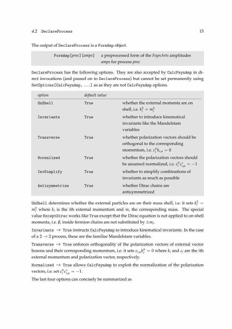
The output of DeclareProcess is a FormAmp object.
FormAmp[proc][amps] a preprocessed form of the FeynArts amplitudes
amps for process proc
DeclareProcess has the following options. They are also accepted by CalcFeynAmp in di-
rect invocations (and passed on to DeclareProcess) but cannot be set permanently using
SetOptions[CalcFeynAmp, ...] as as they are not CalcFeynAmp options.
option default value
OnShell True whether the external momenta are on
shell, i.e. k2i = m2
i
Invariants True whether to introduce kinematical
invariants like the Mandelstam
variables
Transverse True whether polarization vectors should be
orthogonal to the corresponding
momentum, i.e. εµi ki,µ = 0
Normalized True whether the polarization vectors should
be assumed normalized, i.e. εµi ε∗i,µ = −1
InvSimplify True whether to simplify combinations of
invariants as much as possible
Antisymmetrize True whether Dirac chains are
antisymmetrized
OnShell determines whether the external particles are on their mass shell, i.e. it sets k2i =
m2i where ki is the ith external momentum and mi the corresponding mass. The special
value ExceptDirac works like True except that the Dirac equation is not applied to on-shell
momenta, i.e. /ki inside fermion chains are not substituted by ±mi.
Invariants -> True instructs CalcFeynAmp to introduce kinematical invariants. In the case
of a 2 → 2 process, these are the familiar Mandelstam variables.
Transverse -> True enforces orthogonality of the polarization vectors of external vector
bosons and their corresponding momentum, i.e. it sets εi,µkµi = 0 where ki and εi are the ith
external momentum and polarization vector, respectively.
Normalized -> True allows CalcFeynAmp to exploit the normalization of the polarization
vectors, i.e. set εµi ε∗i,µ = −1.
The last four options can concisely be summarized as

16 4 ALGEBRAICALLY SIMPLIFYING DIAGRAMS
Option Action
OnShell -> True ki · ki = m2i
Mandelstam -> True ki · k j = ± 12
[(s|t)i j − m2
i − m2j
]
Transverse -> True εi · ki = 0
Normalized -> True εi ·ε∗i = −1
InvSimplify controls whether CalcFeynAmp should try to simplify combinations of invari-
ants as much as possible.
Antisymmetrize determines whether Dirac chains are antisymmetrized. Note that this does
not affect Weyl chains, i.e. has an effect only if FermionChains -> Chiral or VA is chosen in
CalcFeynAmp. Take care that antisymmetrized and non-antisymmetrized Dirac chains have
an indistinguishable notation. Needless to say, one should not change the antisymmetriza-
tion flag between CalcFeynAmp and HelicityME.
4.3 Clearing, Combining, Selecting
CalcFeynAmp needs no declarations of the kinematics of the underlying process; it uses the
information FeynArts hands down. This is convenient, but it also requires certain care on
the side of the user because of the abbreviations FormCalc automatically introduces in the
result (see Sect. 4.5). Owing to the presence of momenta and polarization vectors, abbrevi-
ations introduced for different processes will in general have different values, even if they
have the same analytical form. To ensure that processes with different kinematics cannot
be mixed accidentally, CalcFeynAmp refuses to calculate amplitudes belonging to a process
whose kinematics differ from those of the last calculation unless ClearProcess[] is invoked
in between.
ClearProcess[] removes internal definitions before calculating a
new process
The Combine function combines amplitudes. It works before and after CalcFeynAmp, i.e.
on either FeynAmpList or Amp objects. When trying to combine amplitudes from different
processes, Combine issues a warning only, but does not refuse to work as CalcFeynAmp.
Combine[amp1, amp2, . . . ] combines amp1, amp2, . . .
The following two functions are helpful to select diagrams.

4.3 Clearing, Combining, Selecting 17
FermionicQ[d] True if diagram d contains fermions
DiagramType[d] returns the number of propagators in diagram d not
belonging to the loop
FermionicQ is used for selecting diagrams that contain fermions, i.e.
ferm = CalcFeynAmp[ Select[amps, FermionicQ] ]
DiagramType returns the number of propagators not containing the integration momentum.
To see how this classifies diagrams, imagine a 2 → 2 process without self-energy insertions
on external legs (i.e. in an on-shell renormalization scheme). There, DiagramType gives 2 for
a self-energy diagram, 1 for a vertex-correction diagram, and 0 for a box diagram, so that for
instance
vert = CalcFeynAmp[ Select[amps, DiagramType[#] == 1 &] ]
calculates all vertex corrections. DiagramType is of course only a very crude way of clas-
sifying diagrams and not nearly as powerful as the options available in FeynArts, like
ExcludeTopologies.
Individual legs can be taken off-shell with the function OffShell.
OffShell[amp, i -> µi, . . . ] enforce the relation p2i = µ2
i on the amplitudes amp.
OffShell[amp, i -> µi, j -> µ j, . . . ] takes legs i, j, . . . off-shell by substituting the rela-
tion p2i = µ2
i for the true on-shell relation p2i = m2
i . This is unlike the CalcFeynAmp option
OnShell -> False which takes all legs off-shell by not using p2i = m2
i at all.
Finally, the following two functions serve to add factors to particular diagrams.
MultiplyDiagrams[f][amps] multiply the diagrams in amps with the factor
returned by the function f
TagDiagrams[amp] multiply each diagram in amp with the identifier
Diagram[n], where n is the diagram’s number
MultiplyDiagrams[f][amp] multiplies the diagrams in amp with factors depending on their
contents. The factor is determined by the function f which is applied to each diagram either
as f [amplitude], for fully inserted diagrams, or f [generic amplitude, insertion]. For example,
to add a QCD enhancement factor to all diagrams containing a quark mass, the following
function could be used as MultiplyDiagrams[QCDfactor][amps]:
QCDfactor[args__] := QCDenh /; !FreeQ[args, Mf[3|4, __]]
_QCDfactor = 1
18 4 ALGEBRAICALLY SIMPLIFYING DIAGRAMS
TagDiagrams is a special case of MultiplyDiagrams and multiplies each diagram with an
identifier of the form Diagram[n], where n is the diagram’s running number. This provides
is very simple mechanism to identify the origin of terms in the final amplitude.
4.4 Ingredients of Feynman amplitudes
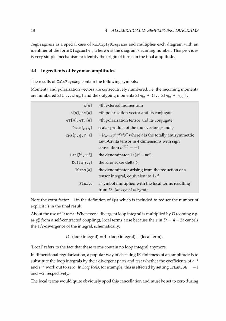
The results of CalcFeynAmp contain the following symbols:
Momenta and polarization vectors are consecutively numbered, i.e. the incoming momenta
are numbered k[1]. . . k[nin] and the outgoing momenta k[nin + 1]. . . k[nin + nout].
k[n] nth external momentum
e[n], ec[n] nth polarization vector and its conjugate
eT[n], eTc[n] nth polarization tensor and its conjugate
Pair[p, q] scalar product of the four-vectors p and q
Eps[p, q, r, s] −iεµνρσpµqνrρsσ where ε is the totally antisymmetric
Levi-Civita tensor in 4 dimensions with sign
convention ε0123 = +1
Den[k2,m2] the denominator 1/(k2 − m2)
Delta[i, j] the Kronecker delta δij
IGram[d] the denominator arising from the reduction of a
tensor integral, equivalent to 1/d
Finite a symbol multiplied with the local terms resulting
from D · (divergent integral)
Note the extra factor −i in the definition of Eps which is included to reduce the number of
explicit i’s in the final result.
About the use of Finite: Whenever a divergent loop integral is multiplied by D (coming e.g.
as gµµ from a self-contracted coupling), local terms arise because the ε in D = 4 − 2ε cancels
the 1/ε-divergence of the integral, schematically:
D · (loop integral) = 4 · (loop integral) + (local term) .
‘Local’ refers to the fact that these terms contain no loop integral anymore.
In dimensional regularization, a popular way of checking IR-finiteness of an amplitude is to
substitute the loop integrals by their divergent parts and test whether the coefficients of ε−1
andε−2 work out to zero. In LoopTools, for example, this is effected by setting LTLAMBDA = −1
and −2, respectively.
The local terms would quite obviously spoil this cancellation and must be set to zero during
4.4 Ingredients of Feynman amplitudes 19
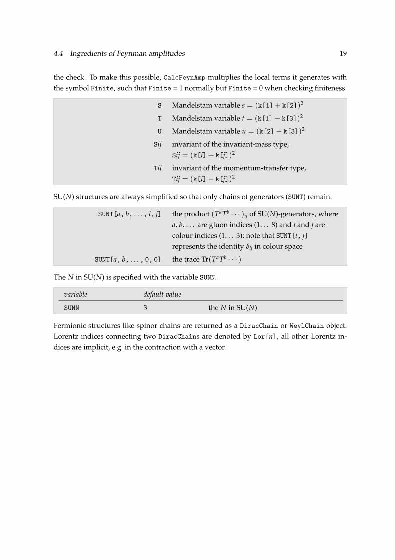
the check. To make this possible, CalcFeynAmp multiplies the local terms it generates with
the symbol Finite, such that Finite = 1 normally but Finite = 0 when checking finiteness.
S Mandelstam variable s = (k[1]+ k[2])2
T Mandelstam variable t = (k[1]− k[3])2
U Mandelstam variable u = (k[2]− k[3])2
Sij invariant of the invariant-mass type,
Sij = (k[i]+ k[j])2
Tij invariant of the momentum-transfer type,
Tij = (k[i]− k[j])2
SU(N) structures are always simplified so that only chains of generators (SUNT) remain.
SUNT[a, b, . . . , i, j] the product (TaTb · · · )ij of SU(N)-generators, where
a, b, . . . are gluon indices (1. . . 8) and i and j are
colour indices (1. . . 3); note that SUNT[i, j]
represents the identity δij in colour space
SUNT[a, b, . . . , 0, 0] the trace Tr(TaTb · · · )
The N in SU(N) is specified with the variable SUNN.
variable default value
SUNN 3 the N in SU(N)
Fermionic structures like spinor chains are returned as a DiracChain or WeylChain object.
Lorentz indices connecting two DiracChains are denoted by Lor[n], all other Lorentz in-
dices are implicit, e.g. in the contraction with a vector.
20 4 ALGEBRAICALLY SIMPLIFYING DIAGRAMS
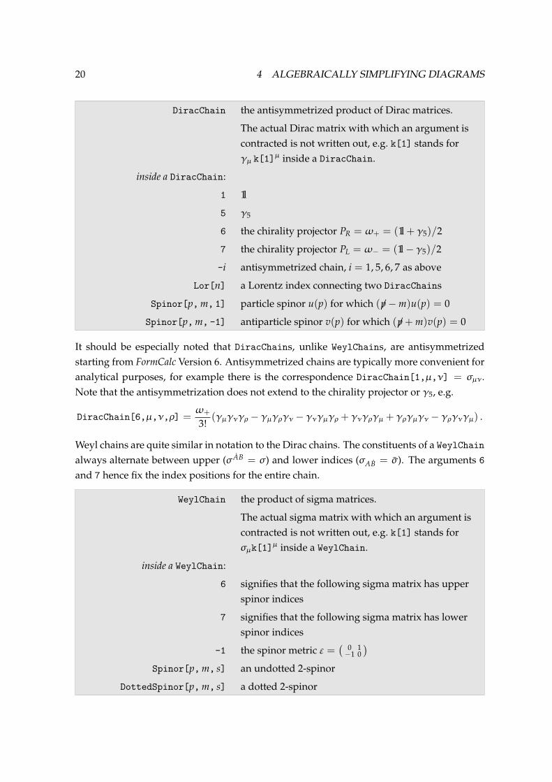
DiracChain the antisymmetrized product of Dirac matrices.
The actual Dirac matrix with which an argument is
contracted is not written out, e.g. k[1] stands for
γµ k[1]µ inside a DiracChain.
inside a DiracChain:
1 1l
5 γ5
6 the chirality projector PR = ω+ = (1l + γ5)/2
7 the chirality projector PL = ω− = (1l −γ5)/2
-i antisymmetrized chain, i = 1, 5, 6, 7 as above
Lor[n] a Lorentz index connecting two DiracChains
Spinor[p, m, 1] particle spinor u(p) for which (/p − m)u(p) = 0
Spinor[p,m, -1] antiparticle spinor v(p) for which (/p + m)v(p) = 0
It should be especially noted that DiracChains, unlike WeylChains, are antisymmetrized
starting from FormCalc Version 6. Antisymmetrized chains are typically more convenient for
analytical purposes, for example there is the correspondence DiracChain[1,µ,ν] = σµν .
Note that the antisymmetrization does not extend to the chirality projector or γ5, e.g.
DiracChain[6,µ,ν,ρ] =ω+
3!(γµγνγρ − γµγργν − γνγµγρ + γνγργµ + γργµγν − γργνγµ) .
Weyl chains are quite similar in notation to the Dirac chains. The constituents of a WeylChain
always alternate between upper (σ AB = σ) and lower indices (σAB = σ). The arguments 6
and 7 hence fix the index positions for the entire chain.
WeylChain the product of sigma matrices.
The actual sigma matrix with which an argument is
contracted is not written out, e.g. k[1] stands for
σµk[1]µ inside a WeylChain.
inside a WeylChain:
6 signifies that the following sigma matrix has upper
spinor indices
7 signifies that the following sigma matrix has lower
spinor indices
-1 the spinor metric ε =(
0 1−1 0
)
Spinor[p,m, s] an undotted 2-spinor
DottedSpinor[p, m, s] a dotted 2-spinor
4.4 Ingredients of Feynman amplitudes 21
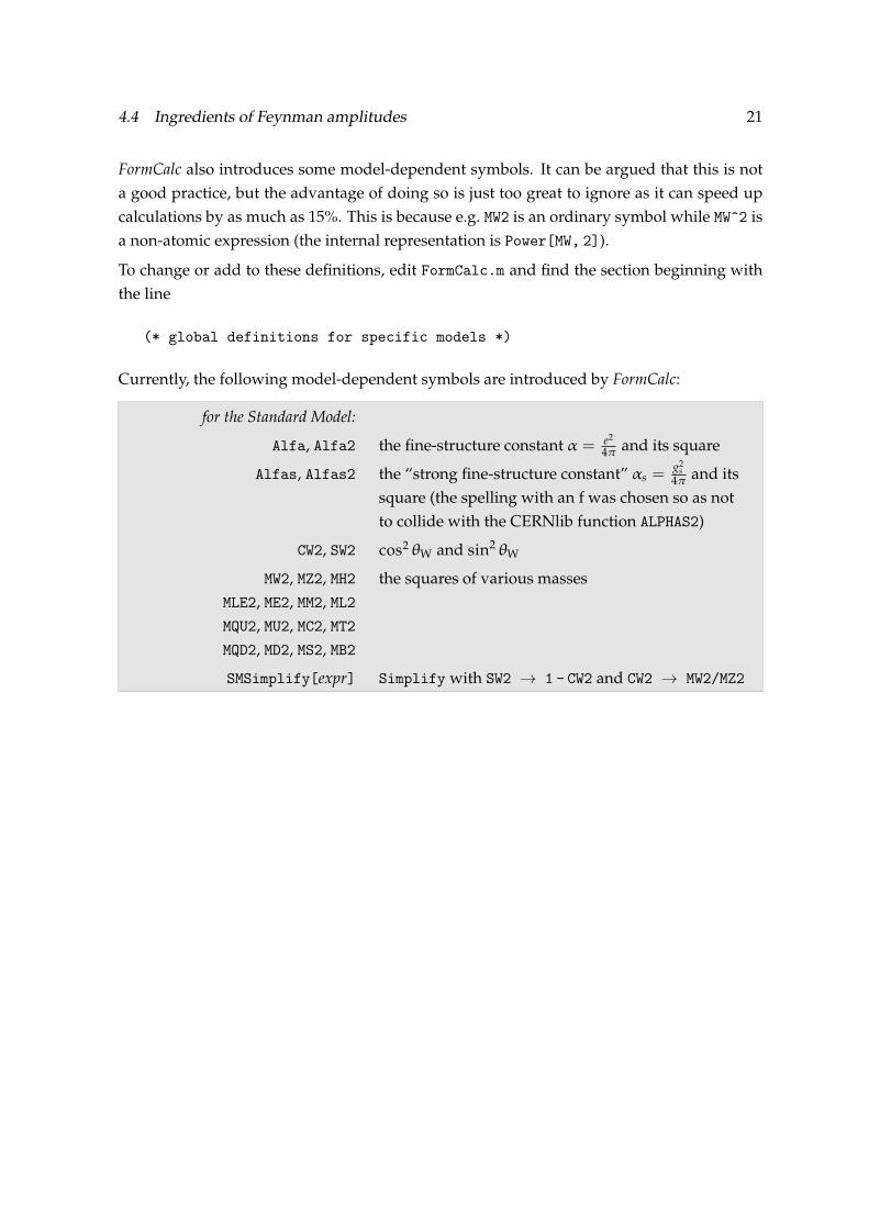
FormCalc also introduces some model-dependent symbols. It can be argued that this is not
a good practice, but the advantage of doing so is just too great to ignore as it can speed up
calculations by as much as 15%. This is because e.g. MW2 is an ordinary symbol while MW^2 is
a non-atomic expression (the internal representation is Power[MW, 2]).
To change or add to these definitions, edit FormCalc.m and find the section beginning with
the line
(* global definitions for specific models *)
Currently, the following model-dependent symbols are introduced by FormCalc:
for the Standard Model:
Alfa, Alfa2 the fine-structure constantα = e2
4π and its square
Alfas, Alfas2 the “strong fine-structure constant”αs =g2
s4π and its
square (the spelling with an f was chosen so as not
to collide with the CERNlib function ALPHAS2)
CW2, SW2 cos2θW and sin2θW
MW2, MZ2, MH2
MLE2, ME2, MM2, ML2
MQU2, MU2, MC2, MT2
MQD2, MD2, MS2, MB2
the squares of various masses
SMSimplify[expr] Simplify with SW2 → 1 - CW2 and CW2 → MW2/MZ2

22 4 ALGEBRAICALLY SIMPLIFYING DIAGRAMS
for the MSSM:
CA2, SA2, CB2, SB2, TB2 cos2α, sin2α, cos2 β, sin2 β, and tan2 β
CBA2, SBA2 cos2(β−α), sin2(β−α)
USfC, UChaC, VChaC, ZNeuC the complex conjugates of various mixing matrix
elements
MGl2, MSf2, MCha2, MNeu2
Mh02, MHH2, MA02
MG02, MHp2, MGp2
the squares of various masses
MSSMSimplify[expr] Simplify with SUSY trigonometric identities
(e.g. SBA2 → 1 - CBA2)
SUSYTrigExpand[expr] express various trigonometric symbols
(SB2, S2B, etc.) through ca, sa, cb, sb
SUSYTrigReduce[expr] substitute back ca, sa, cb, sb
SUSYTrigSimplify[expr] perform trigonometric simplifications by applying
SUSYTrigExpand, Simplify, and SUSYTrigReduce in
sequence
Often one wants to neglect certain variables, typically masses. Directly defining, say, ME = 0
may lead to problems, however, for instance if ME appears in a negative power, or in loop
integrals where neglecting it may cause singularities. A better way is to assign values to
the function Neglect, e.g. Neglect[ME] = 0, which allows FormCalc to replace ME by zero
whenever this is safe. Watch out for the built-in definitions mentioned above: since e.g. ME^2
is automatically replaced by ME2, one has to assign Neglect[ME] = Neglect[ME2] = 0 in
order to have also the even powers of the electron mass neglected.
Neglect[s] = 0 replace s by 0 except when it appears in negative
powers or in loop integrals
To a certain extent it is also possible to use patterns in the argument of Neglect. Simple
patterns like _ and __ work always. Since FORM’s pattern matching is far inferior to Mathe-
matica’s, though, it is not at all difficult to come up with patterns which are not accepted by
FORM.
Determining the mass dimension is an easy way of checking consistency of an expression.
The function MassDim substitutes all symbols in the list MassDim0 by a random number, all
symbols in MassDim1 by Mass times a random number, and all symbols in MassDim2 by Mass2
times a random number. Symbols not in MassDim0,1,2 are not replaced. The random
numbers are supposed to guard against accidental cancellations. An expression consistent
in the mass dimension should end up with just one term of the form (number) · Massn.

4.5 Handling Abbreviations 23
MassDim[expr] replace the MassDimn-symbols in expr by
(random number) · Massn
MassDim0 a list of symbols of mass dimension 0
MassDim1 a list of symbols of mass dimension 1
MassDim2 a list of symbols of mass dimension 2
Mass a symbol representing the mass dimension
4.5 Handling Abbreviations
CalcFeynAmp returns expressions where spinor chains, dot products of vectors, and Levi-
Civita tensors contracted with vectors have been collected and abbreviated. A term in such
an expression may look like
C0i[cc12, MW2, MW2, S, MW2, MZ2, MW2] *
( -4 AbbSum16 Alfa2 CW2 MW2 S/SW2 + 32 AbbSum28 Alfa2 CW2 S^2/SW2 +
4 AbbSum30 Alfa2 CW2 S^2/SW2 - 8 AbbSum7 Alfa2 CW2 S^2/SW2 +
Abb1 Alfa2 CW2 S (T - U)/SW2 + 8 AbbSum29 Alfa2 CW2 S (T - U)/SW2 )
The first line stands for the tensor-coefficient function C12(M2W, M2
W, s, M2W , M2
Z, M2W) which
is multiplied with a linear combination of abbreviations like Abb1 or AbbSum28 with certain
coefficients. The coefficients of the abbreviations contain kinematical variables, in this case
the Mandelstam variables S, T, and U, and parameters of the model, here e.g. Alfa2 or MW2.
This particular excerpt of code happens to be from a process without external fermions;
otherwise spinor chains, abbreviated as Fn, would appear, too.
The abbreviations like Abb1 or AbbSum29 can drastically reduce the size of an amplitude,
particularly so because they are nested in three levels. Consider AbbSum29 from the example
above, which is an abbreviation of about average length:
AbbSum29 = Abb2 + Abb22 + Abb23 + Abb3
Abb22 = Pair1 Pair3 Pair6
Pair3 = Pair[e[3], k[1]]
Without abbreviations, the result would for each AbbSum29 contain
Pair[e[1], e[2]] Pair[e[3], k[1]] Pair[e[4], k[1]] +
Pair[e[1], e[2]] Pair[e[3], k[2]] Pair[e[4], k[1]] +
Pair[e[1], e[2]] Pair[e[3], k[1]] Pair[e[4], k[2]] +
Pair[e[1], e[2]] Pair[e[3], k[2]] Pair[e[4], k[2]]
24 4 ALGEBRAICALLY SIMPLIFYING DIAGRAMS
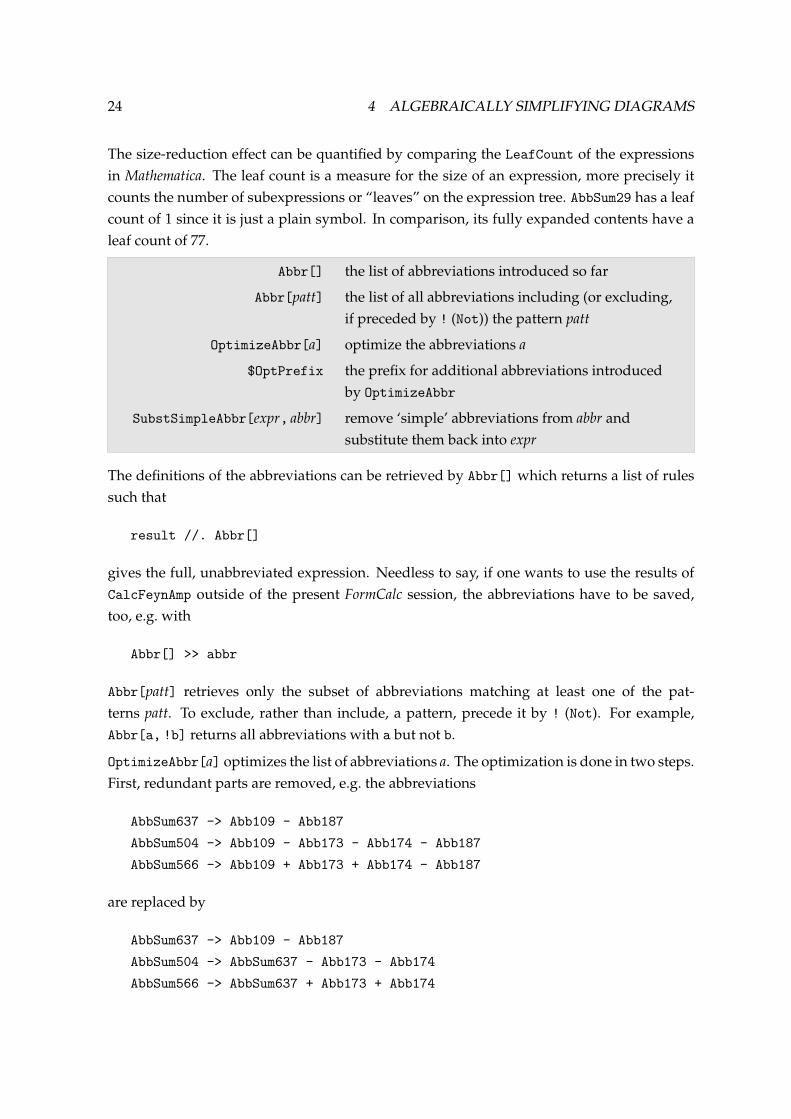
The size-reduction effect can be quantified by comparing the LeafCount of the expressions
in Mathematica. The leaf count is a measure for the size of an expression, more precisely it
counts the number of subexpressions or “leaves” on the expression tree. AbbSum29 has a leaf
count of 1 since it is just a plain symbol. In comparison, its fully expanded contents have a
leaf count of 77.
Abbr[] the list of abbreviations introduced so far
Abbr[patt] the list of all abbreviations including (or excluding,
if preceded by ! (Not)) the pattern patt
OptimizeAbbr[a] optimize the abbreviations a
$OptPrefix the prefix for additional abbreviations introduced
by OptimizeAbbr
SubstSimpleAbbr[expr, abbr] remove ‘simple’ abbreviations from abbr and
substitute them back into expr
The definitions of the abbreviations can be retrieved by Abbr[] which returns a list of rules
such that
result //. Abbr[]
gives the full, unabbreviated expression. Needless to say, if one wants to use the results of
CalcFeynAmp outside of the present FormCalc session, the abbreviations have to be saved,
too, e.g. with
Abbr[] >> abbr
Abbr[patt] retrieves only the subset of abbreviations matching at least one of the pat-
terns patt. To exclude, rather than include, a pattern, precede it by ! (Not). For example,
Abbr[a, !b] returns all abbreviations with a but not b.
OptimizeAbbr[a] optimizes the list of abbreviations a. The optimization is done in two steps.
First, redundant parts are removed, e.g. the abbreviations
AbbSum637 -> Abb109 - Abb187
AbbSum504 -> Abb109 - Abb173 - Abb174 - Abb187
AbbSum566 -> Abb109 + Abb173 + Abb174 - Abb187
are replaced by
AbbSum637 -> Abb109 - Abb187
AbbSum504 -> AbbSum637 - Abb173 - Abb174
AbbSum566 -> AbbSum637 + Abb173 + Abb174
4.6 More Abbreviations 25
Then, in a second step, common subexpressions are eliminated, thereby simplifying the last
lines further to
AbbSum637 -> Abb109 - Abb187
Opt1 -> Abb173 + Abb174
AbbSum504 -> AbbSum637 - Opt1
AbbSum566 -> AbbSum637 + Opt1
Optimizing the abbreviations may take some time but can also speed up numerical com-
putations considerably. The prefix for the new abbreviations introduced by OptimizeAbbr,
i.e. the Opt in the OptN in the example above, can be chosen through the global variable
$OptPrefix.
SubstSimpleAbbr[expr, abbr] removes ‘simple’ abbreviations the list of abbreviations abbr
and substitutes them back into expr. Abbreviations of the form (number) and (number) ·(symbol) are considered simple. Such expressions may show up in the abbreviation list e.g.
after further simplification.
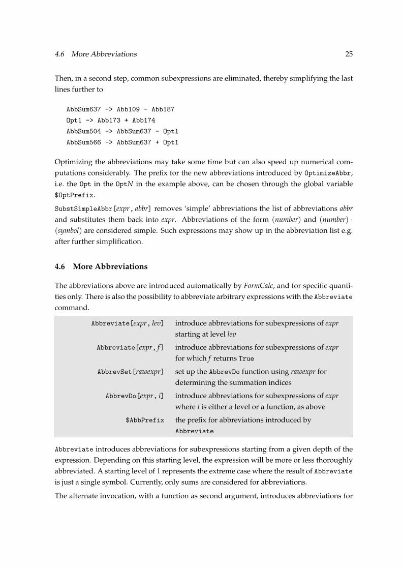
4.6 More Abbreviations
The abbreviations above are introduced automatically by FormCalc, and for specific quanti-
ties only. There is also the possibility to abbreviate arbitrary expressions with the Abbreviate
command.
Abbreviate[expr, lev] introduce abbreviations for subexpressions of expr
starting at level lev
Abbreviate[expr, f] introduce abbreviations for subexpressions of expr
for which f returns True
AbbrevSet[rawexpr] set up the AbbrevDo function using rawexpr for
determining the summation indices
AbbrevDo[expr, i] introduce abbreviations for subexpressions of expr
where i is either a level or a function, as above
$AbbPrefix the prefix for abbreviations introduced by
Abbreviate
Abbreviate introduces abbreviations for subexpressions starting from a given depth of the
expression. Depending on this starting level, the expression will be more or less thoroughly
abbreviated. A starting level of 1 represents the extreme case where the result of Abbreviate
is just a single symbol. Currently, only sums are considered for abbreviations.
The alternate invocation, with a function as second argument, introduces abbreviations for

26 4 ALGEBRAICALLY SIMPLIFYING DIAGRAMS
all subexpressions for which this function yields True, like Select. This is useful, for ex-
ample, to get a picture of the structure of an expression with respect to a certain object, as
in
Abbreviate[a + b + c + (d + e) x, FreeQ[#, x]&, MinLeafCount -> 0]
which gives Sub2 + Sub1 x, thus indicating that the original expression is linear in x.
The functionality of Abbreviate is actually separated into a pair of functions AbbrevSet and
AbbrevDo, i.e. Abbreviate internally runs AbbrevSet to define AbbrevDo and then executes
AbbrevDo. The expression given to AbbrevSet is not itself abbreviated but used for determin-
ing the summation indices; it could be e.g. a raw amplitude. This is particularly important
in cases where partial expressions will be given to AbbrevDo and where the summation in-
dices may not be correctly inferred because AbbrevDo does not see the full expression. The
definition of AbbrevDo is not automatically removed, so be careful not to execute AbbrevDo
with an expression that is not a subexpression of the one given to AbbrevSet!
The prefix of the abbreviations are given by the global variable $AbbPrefix.
option default value
MinLeafCount 10 the mininum leaf count above which a
subexpression becomes eligible for
abbreviationing
Deny k, q1 symbols which must not occur in
abbreviations
Fuse True whether to fuse adjacent items for
which the selection function is True into
one abbreviation
Preprocess Identity a function applied to subexpressions
before abbreviationing
MinLeafCount determines the minimum leaf count a common subexpression must have in
order that a variable is introduced for it.
Deny specifies an exclusion list of symbols which must not occur in abbreviations.
Fuse specifies whether adjacent items for which the selection function returns True should
be fused into one abbreviation. It has no effect when Abbreviate is invoked with a depth.
For example,
Abbreviate[a Pair[1, 2] Pair[3, 4], MatchQ[#, _Pair]&,
Fuse -> False, MinLeafCount -> 0]
introduces two abbreviations, one for Pair[1, 2] and one for Pair[3, 4], whereas with
4.7 Resuming Previous Sessions 27
Fuse -> True only one abbreviation for the product is introduced.
Preprocess specifies a function to be applied to all subexpressions before introducing ab-
breviations for them.
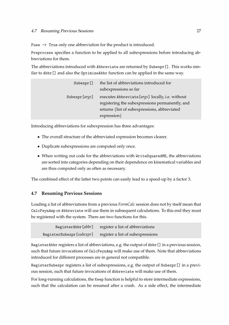
The abbreviations introduced with Abbreviate are returned by Subexpr[]. This works sim-
ilar to Abbr[] and also the OptimizeAbbr function can be applied in the same way.
Subexpr[] the list of abbreviations introduced for
subexpressions so far
Subexpr[args] executes Abbreviate[args] locally, i.e. without
registering the subexpressions permanently, and
returns list of subexpressions, abbreviated
expression
Introducing abbreviations for subexpression has three advantages:
• The overall structure of the abbreviated expression becomes clearer.
• Duplicate subexpressions are computed only once.
• When writing out code for the abbreviations with WriteSquaredME, the abbreviations
are sorted into categories depending on their dependence on kinematical variables and
are thus computed only as often as necessary.
The combined effect of the latter two points can easily lead to a speed-up by a factor 3.
4.7 Resuming Previous Sessions
Loading a list of abbreviations from a previous FormCalc session does not by itself mean that
CalcFeynAmp or Abbreviate will use them in subsequent calculations. To this end they must
be registered with the system. There are two functions for this.
RegisterAbbr[abbr] register a list of abbreviations
RegisterSubexpr[subexpr] register a list of subexpressions
RegisterAbbr registers a list of abbreviations, e.g. the output of Abbr[] in a previous session,
such that future invocations of CalcFeynAmp will make use of them. Note that abbreviations
introduced for different processes are in general not compatible.
RegisterSubexpr registers a list of subexpressions, e.g. the output of Subexpr[] in a previ-
ous session, such that future invocations of Abbreviate will make use of them.
For long-running calculations, the Keep function is helpful to store intermediate expressions,
such that the calculation can be resumed after a crash. As a side effect, the intermediate
28 4 ALGEBRAICALLY SIMPLIFYING DIAGRAMS
results can be inspected easily, even while a batch job is in progress.
Keep[expr, name, path] loads path/name.m if it exists, otherwise evaluates
expr and stores the result (together with the output
of Abbr[] and Subexpr[]) in that file. path is
optional and defaults to $KeepDir
Keep[expr, name] same as Keep[expr, name, $KeepDir]
Keep[lhs = rhs] same as lhs = Keep[rhs, "lhs"]
$KeepDir the default directory for storing intermediate
expressions
Keep has two basic arguments: a file (path and name) and an expression. If the file exists, it
is loaded. If not, the expression is evaluated and the results stored in the file, thus creating
a checkpoint. If the calculation crashes, it suffices to restart the very same program, which
will then load all parts of the calculation that have been completed and resume at the point
it left off.
The syntax of Keep is constructed so as to make adding it to existing programs is as painless
as possible. For example, a statement like
amps = CalcFeynAmp[...]
simply becomes
Keep[amps = CalcFeynAmp[...]]
Needless to say, this logic fails to work if symbols are being re-assigned, i.e. appear more
than once on the left-hand side, as in
Keep[amps = CalcFeynAmp[virt]]
Keep[amps = Join[amps, CalcFeynAmp[counter]]
Due to the first Keep statement, the second will always find the file keep/amps.m and never
execute the computation of the counter terms.
And there are other ways to confuse the system: mixing intermediate results from different
calculations, changing flags out of sync with the intermediate results, etc. In case of doubt,
i.e. if results seem suspicious, remove all intermediate files and re-do the calculation from
scratch.
4.8 Fermionic Matrix Elements
When FermionChains -> Chiral or VA is chosen, an amplitude involving external fermions
will contain DiracChains, abbreviated as Fi, e.g.
4.8 Fermionic Matrix Elements 29
F1 -> DiracChain[Spinor[k[2], ME, -1], 6, Lor[1], Spinor[k[1], ME, 1]] *
DiracChain[Spinor[k[3], MT, 1], 6, Lor[1], Spinor[k[4], MT, -1]]
In physical observables such as the cross-section, where only the square of the amplitude
or interference terms can enter, these spinor chains can be evaluated without reference to a
concrete representation for the spinors. The point is that in terms like |M|2 or 2 Re(M1M∗2)
only products (Fi Fj) of spinor chains appear and these can be calculated using the density
matrix for spinors
uλ(p)uλ(p), vλ(p)vλ(p) =
12 (1 ± λγ5)/p for massless fermions†
12 (1 + λγ5/s)(/p ± m) for massive fermions
where λ = ± and s is the helicity reference vector corresponding to the momentum p. s
is the unit vector in the direction of the spin axis in the particle’s rest frame, boosted into
the CMS. It is identical to the longitudinal polarization vector of a vector boson, and fulfills
s · p = 0 and s2 = −1.
In the unpolarized case the λ-dependent part adds up to zero, so the projectors become
∑λ=±
uλ(p)uλ(p) = /p + m , ∑λ=±
vλ(p)vλ(p) = /p − m .
Technically, one can use the same formula as in the polarized case by putting λ = 0 and
multiplying the result by 2 for each external fermion.
FormCalc supplies the function HelicityME to calculate these so-called helicity matrix ele-
ments (Fi Fj).
†In the limit E ≫ m the vector s becomes increasingly parallel to p, i.e. s ∼ p/m, hence
/p(/p + m) = p2 + m/p = m(/p + m)
/p(/p − m) = p2 − m/p = −m(/p − m)
⇒ (1 + λγ5/s)(/p ± m)
E≫m−→(
1 + λγ5/p
m
)(/p ± m) = (1 ± λγ5)/p .

30 4 ALGEBRAICALLY SIMPLIFYING DIAGRAMS
HelicityME[M1,M∗2] calculate the helicity matrix elements for all
combinations of Fn appearing in M1 and M∗2,
where, as the ∗ indicates, M2 is the part to be
complex conjugated
All (used as an argument of HelicityME:) instead of
selecting the Fs which appear in an expression,
simply take all Fs currently in the abbreviations
Mat[Fi, Fj] the helicity matrix element resulting from the
spinor chains in Fi and Fj
Hel[n] the helicity λn of the nth external particle
s[n] the helicity reference vector of the nth external
particle
Note that HelicityME does not calculate the full expression M1M∗2, but only the combina-
tions of Fs that appear in this product. These are then called Mat[Fi, Fj] and depend on the
helicities and helicity reference vectors of the external particles, Hel[n] and s[n]. See Sect.
4.10 on how to put together the complete expression M1M∗2.
If possible, specific values for the Hel[n] should be fixed in advance, since that can dramat-
ically speed up the calculation and also lead to (much) more compact results. For example,
as mentioned before, unpolarized matrix elements can be obtained by putting the helicities
λn = 0 and multiplying by 2 for each external fermion. Therefore, for calculating only the
unpolarized amplitude, one could use
_Hel = 0;
mat = HelicityME[...]
which is generally much faster than HelicityME[...] /. Hel[_] -> 0. (Don’t forget that
the matrix elements obtained in this way have yet to be multiplied by 2 for each external
fermion.)
Note: HelicityME uses internal definitions set up by CalcFeynAmp. It is therefore not ad-
visable to mix the evaluation of different processes. For instance, wrong results can be
expected if one uses HelicityME on results from process A after having computed am-
plitudes from process B with CalcFeynAmp. Since this requires at least one invocation of
ClearProcess, though, it is unlikely to happen accidentally.
4.9 Colour Matrix Elements 31
option default value
Dimension 4 the dimension to compute in
MomElim (taken from
CalcFeynAmp)
how to apply momentum conservation
DotExpand (taken from
CalcFeynAmp)
whether to expand terms collected for
momentum elimination
RetainFile False whether to retain the temporary FORM
command file
EditCode False whether to display the FORM code in
an editor before sending it to FORM
Dimension is used as in CalcFeynAmp. Only the value 0 has the effect of actually computing
in D dimensions, however, since for D and 4 the limit D → 4 has already been taken in
CalcFeynAmp. The dimensional dependence of the result is expressed through Dminus4 and
Dminus4Eps, where the latter represents the Dminus4 arising from the contraction of Levi-
Civita tensors. For testing and comparison, the default equivalence Dminus4Eps = Dminus4
can be unset.
The options MomElim, DotExpand, RetainFile, and EditCode are used in the same way as
for CalcFeynAmp, see page 13.
4.9 Colour Matrix Elements
Diagrams involving quarks or gluons usually‡ contain objects from the SU(N) algebra. These
are simplified by CalcFeynAmp using the Cvitanovic algorithm [Cv76] in an extended version
of the implementation in [Ve96]. The idea is to transform all SU(N) objects to products of
generators Tai j which are generically denoted by SUNT in FormCalc. In the output, only two
types of objects can appear:
• Chains (products) of generators with external colour indices; these are denoted by
SUNT[a, b, . . . , i, j] = (TaTb · · · )ij where i and j are the external colour indices and
the a, b, . . . are the indices of external gluons. This notation includes also the identity
in colour space as the special case with no external gluons: δij = SUNT[i, j].
• Traces over products of generators; these are denoted by SUNT[a, b, . . . , 0, 0] =
Tr(TaTb · · · ).‡Diagrams generated with the SM.mod model file contain no SU(N) objects since in the electroweak sector
colour can be taken care of by a trivial factor 3 for each quark loop.

32 4 ALGEBRAICALLY SIMPLIFYING DIAGRAMS
The situation is much the same as with fermionic structures: just as an amplitude contains
open spinor chains if external fermions are involved, it also contains SUNTs if external quarks
or gluons are involved.
For the SUNT objects in the output, FormCalc introduces abbreviations of the type SUNn. These
abbreviations can easily be evaluated further if one computes the squared amplitude, be-
cause then the external lines close and the Cvitanovic algorithm yields a simple number for
each combination of SUNi and SUNj. (One can think of the squared amplitude being decom-
posed into parts, each of which is multiplied by a different colour factor.) But this is precisely
the idea of helicity matrix elements applied to the SU(N) case!
Because of this close analogy, the combinations of SUNi and SUNj are called colour matrix
elements in FormCalc and are written accordingly as Mat[SUNi, SUNj]. The function which
computes them is ColourME. It is invoked just like HelicityME.
ColourME[M1,M∗2] calculate the colour matrix elements for all
combinations of SUNn appearing in M1 and M∗2,
where, as the ∗ indicates, M2 is the part to be
complex conjugated
All (used as an argument of ColourME:) instead of
selecting the SUNs which appear in an expression,
simply take all SUNs currently in abbreviations
Mat[SUNi, SUNj] the colour matrix element resulting from the SU(N)
objects SUNi and SUNj
The core function behind ColourME can also be used directly to simplify colour structures.
ColourSimplify[expr] simplify colour objects in expr
ColourSimplify[expr, conj] simplifies the colour objects in (expr conj∗)
Furthermore, FormCalc implements a special case of FeynArts’s DiagramGrouping function
in ColourGrouping, which groups Feynman diagrams according to their colour structures.
The correct grouping can only be done with fully simplified colour structures, which is why
this function is part of FormCalc, not FeynArts.
ColourGrouping[ins] group the inserted topologies (output of
InsertFields) according to their colour structures
4.10 Putting together the Squared Amplitude 33
4.10 Putting together the Squared Amplitude
Now that CalcFeynAmp has calculated the amplitudes and HelicityME and ColourME have
produced the helicity and colour matrix elements, the remaining step is to piece together the
squared matrix element |M|2, or more generally products like M1M∗2. For example, M1
could be the sum of the one-loop diagrams and M2 the sum of the tree diagrams.
This is non-trivial only if there are helicity or colour matrix elements Mat[i, j] which have to
be put in the right places. Specifically, if M1 and M2 are written in the form
M1 = a11 F1 SUN1+ a21 F2 SUN1+ . . . = ∑i j
ai j Fi SUN j and
M2 = b11 F1 SUN1+ b21 F2 SUN1+ . . . = ∑i j
bi j Fi SUN j ,
M1M∗2 becomes
M1M∗2 = a11b∗11 Mat[F1, F1] Mat[SUN1, SUN1]+
a21b∗11 Mat[F2, F1] Mat[SUN1, SUN1]+ . . .
= ∑i jkℓ
aikb∗jℓ Mat[Fi, Fj] Mat[SUNk, SUNℓ] .
The coefficients aik and b jℓ are known as form factors. For efficiency, they are usually com-
puted separately in the numerical evaluation, so that the final expression for the squared
matrix element is easily summed up e.g. in Fortran as
do 1 i = 1, (# of Fs in M1)
do 1 j = 1, (# of Fs in M2)
do 1 k = 1, (# of SUNs in M1)
do 1 l = 1, (# of SUNs in M2)
result = result + a(i,k)*DCONJG(b(j,l))*MatF(i,j)*MatSUN(k,l)
1 continue
While this is arguably the most economic way to evaluate a squared amplitude numerically,
it is also possible to directly obtain the squared matrix element as a Mathematica expression.
The function which does this is SquaredME.
SquaredME[M1,M∗2] calculates M1M∗
2 , taking care to put the Mat[i, j] in
the right places
SquaredME is called in much the same way as HelicityME. Because of the number of terms
that are generated, this function is most useful only for rather small amplitudes.
SquaredME does not insert the actual values for the Mat[i, j]. This can easily be done later by
applying the output of HelicityME and ColourME, which are lists of rules substituting the

34 4 ALGEBRAICALLY SIMPLIFYING DIAGRAMS
Mat[i, j] by their values. That is to say, SquaredME and HelicityME or ColourME perform
complementary tasks: SquaredME builds up the squared amplitude in terms of the Mat[i, j]
whereas HelicityME and ColourME calculate the Mat[i, j].
4.11 Polarization Sums
In the presence of external gauge bosons, the output of SquaredME will still contain polar-
ization vectors (in general implicitly, i.e. through the abbreviations). For unpolarized gauge
bosons, the latter can be eliminated by means of the identities
3
∑λ=1
ε∗µ(k, λ)εν(k, λ) = −gµν +kµkνm2
for massive particles,
2
∑λ=1
ε∗µ(k, λ)εν(k, λ) = −gµν −η2kµkν(η · k)2
+ηµkν + ηνkµ
η · kfor massless particles.
In the massless case the polarization sum is gauge dependent and η is an external four-vector
which fulfills η · ε = 0 and η · k 6= 0. For a gauge-invariant quantity, the η-dependence
should ultimately cancel.
FormCalc provides the function PolarizationSum to apply the above identities.
PolarizationSum[expr] sums expr over the polarizations of external gauge
bosons
It is assumed that expr is the squared amplitude into which the helicity matrix elements have
already been inserted. Alternatively, expr may also be given as an amplitude directly, in
which case PolarizationSum will first invoke SquaredME and HelicityME (with _Hel = 0)
to obtain the squared amplitude. PolarizationSum cannot simplify Weyl chains, such as
CalcFeynAmp introduces with FermionChains -> Weyl (the default).

4.11 Polarization Sums 35
option default value
SumLegs All which external legs to include in the
polarization sum
Dimension 4 the dimension to compute in
GaugeTerms True whether to drop the η-dependent terms
MomElim (taken from
CalcFeynAmp)
how to apply momentum conservation
DotExpand (taken from
CalcFeynAmp)
whether to expand terms collected for
momentum elimination
NoBracket (taken from
CalcFeynAmp)
symbols not to be included in the
bracketing in FORM
RetainFile False whether to retain the temporary FORM
command file
EditCode False whether to display the FORM code in
an editor before sending it to FORM
SumLegs allows to restrict the polarization sum to fewer than all external vector bosons. For
example, SumLegs -> 3,4 sums only vector bosons on legs 3 and 4.
Dimension is used as in CalcFeynAmp. Only the value 0 has the effect of actually computing
in D dimensions, however, since for D and 4 the limit D → 4 has already been taken in
CalcFeynAmp. The dimensional dependence of the result is expressed through Dminus4 and
Dminus4Eps, where the latter represents the Dminus4 arising from the contraction of Levi-
Civita tensors. For testing and comparison, the default equivalence Dminus4Eps = Dminus4
can be unset.
GaugeTerms drops terms containing the gauge-dependent auxiliary vector η. More precisely,
the η-terms are actually introduced at first, to let potential cancellations of η’s in the numer-
ator against the denominator occur, but set to zero later.
The options MomElim, DotExpand, NoBracket, RetainFile, and EditCode are used in the
same way as for CalcFeynAmp, see page 13.
Note: PolarizationSum uses internal definitions set up by CalcFeynAmp. It is therefore not
advisable to mix the evaluation of different processes. For instance, wrong results can be
expected if one uses PolarizationSum on results from process A after having computed
amplitudes from process B with CalcFeynAmp. Since this requires at least one invocation of
ClearProcess, though, it is unlikely to happen accidentally.

36 4 ALGEBRAICALLY SIMPLIFYING DIAGRAMS
4.12 Analytic Unsquared Amplitudes
The ‘smallest’ object appearing in the output of CalcFeynAmp is a four-vector, i.e. FormCalc
does not normally go into components. Those are usually inserted only in the numerical
part. This has advantages: for example, the analytical expression does not reflect a particular
phase-space parameterization.
One can also obtain an analytic expression in terms of kinematic invariants (but no four-
vectors) by squaring the amplitude and computing the polarization sums, as outlined above.
This has the advantage of being independent of the representation of the spinors and vectors,
but of course the size of the expression is roughly doubled by squaring.
As a third alternative, one can obtain an analytical expression for the unsquared amplitude.
This requires to go into components, however.
To this end one has to load the extra package VecSet:
<< FormCalc‘tools‘VecSet‘
and for each external vector invoke the function VecSet, which has the same syntax as its
Fortran namesake, e.g.
VecSet[1, m1, p1, 0, 0, 1]
VecSet[n,m, p, ex,ey,ez] set the momentum, polarization vectors, and
spinors for particle n with mass m and
three-momentum p = p ex, ey, ez
The amplitude is then evaluated with the function ToComponents, e.g.
ToComponents[amp, "+-+-"]
This delivers an expression in terms of the phase-space parameters used in VecSet.
ToComponents[amp, "p1p2. . . pn"]
ToComponents[amp, p1, p2,. . . , pn]
evaluate amp by substituting four-vectors by their
component-wise representation using external
polarizations p1, . . . , pn
ToComponents[amp, pol] actually plugs the components of the four-vectors and spinors into
the amplitude amp. The external polarizations pol can be given either as a string with el-
ements +, -, 0 for right-handed, left-handed, and longitudinal polarization, or as a list of
integers +1, -1, 0.
4.13 Checking Ultraviolet Finiteness 37
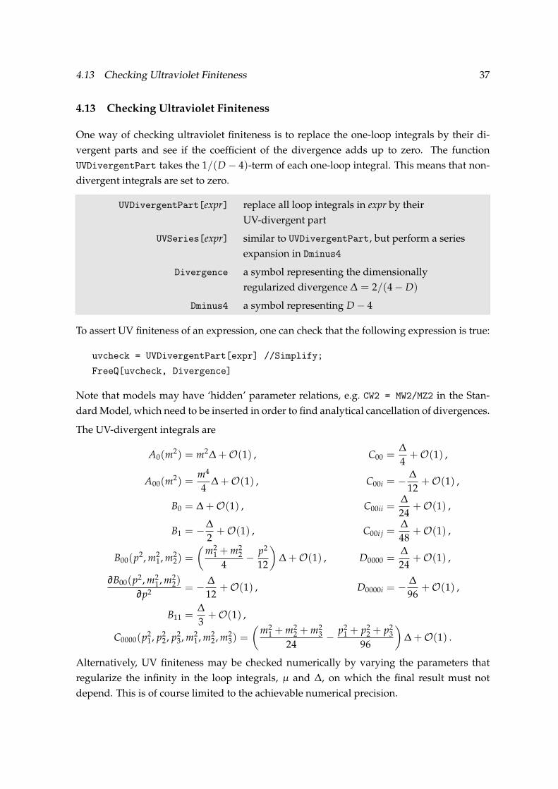
4.13 Checking Ultraviolet Finiteness
One way of checking ultraviolet finiteness is to replace the one-loop integrals by their di-
vergent parts and see if the coefficient of the divergence adds up to zero. The function
UVDivergentPart takes the 1/(D − 4)-term of each one-loop integral. This means that non-
divergent integrals are set to zero.
UVDivergentPart[expr] replace all loop integrals in expr by their
UV-divergent part
UVSeries[expr] similar to UVDivergentPart, but perform a series
expansion in Dminus4
Divergence a symbol representing the dimensionally
regularized divergence ∆ = 2/(4 − D)
Dminus4 a symbol representing D − 4
To assert UV finiteness of an expression, one can check that the following expression is true:
uvcheck = UVDivergentPart[expr] //Simplify;
FreeQ[uvcheck, Divergence]
Note that models may have ‘hidden’ parameter relations, e.g. CW2 = MW2/MZ2 in the Stan-
dard Model, which need to be inserted in order to find analytical cancellation of divergences.
The UV-divergent integrals are
A0(m2) = m2∆+O(1) , C00 =
∆
4+O(1) ,
A00(m2) =
m4
4∆+O(1) , C00i = − ∆
12+O(1) ,
B0 = ∆+O(1) , C00ii =∆
24+O(1) ,
B1 = −∆
2+O(1) , C00i j =
∆
48+O(1) ,
B00(p2, m21, m2
2) =
(m2
1 + m22
4− p2
12
)∆+O(1) , D0000 =
∆
24+O(1) ,
∂B00(p2, m21, m2
2)
∂p2= − ∆
12+O(1) , D0000i = − ∆
96+O(1) ,
B11 =∆
3+O(1) ,
C0000(p21, p2
2, p23, m2
1, m22, m2
3) =
(m2
1 + m22 + m2
3
24− p2
1 + p22 + p2
3
96
)∆+O(1) .
Alternatively, UV finiteness may be checked numerically by varying the parameters that
regularize the infinity in the loop integrals, µ and ∆, on which the final result must not
depend. This is of course limited to the achievable numerical precision.
38 4 ALGEBRAICALLY SIMPLIFYING DIAGRAMS
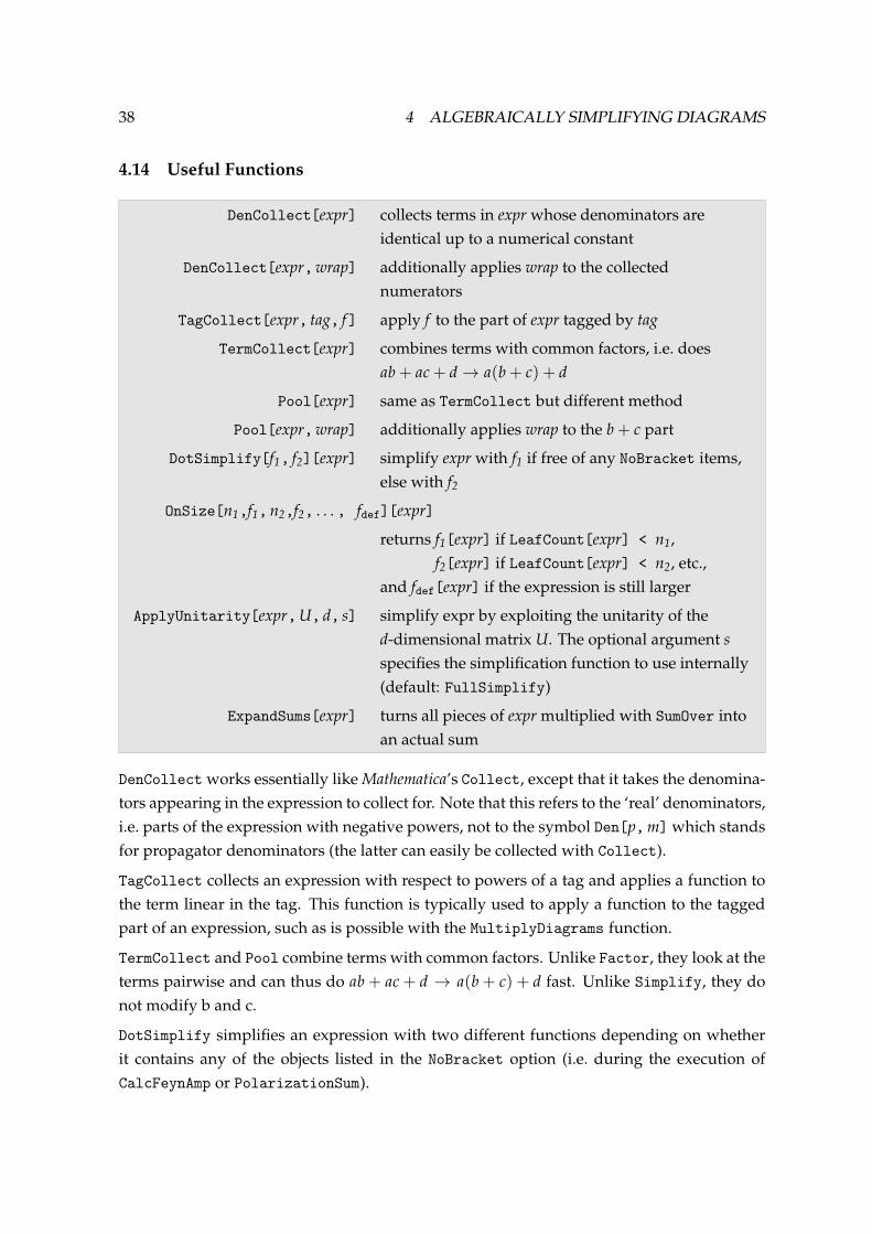
4.14 Useful Functions
DenCollect[expr] collects terms in expr whose denominators are
identical up to a numerical constant
DenCollect[expr,wrap] additionally applies wrap to the collected
numerators
TagCollect[expr, tag, f] apply f to the part of expr tagged by tag
TermCollect[expr] combines terms with common factors, i.e. does
ab + ac + d → a(b + c) + d
Pool[expr] same as TermCollect but different method
Pool[expr,wrap] additionally applies wrap to the b + c part
DotSimplify[f1, f2][expr] simplify expr with f1 if free of any NoBracket items,
else with f2
OnSize[n1,f1, n2,f2, . . . , fdef][expr]
returns f1[expr] if LeafCount[expr] < n1,
f2[expr] if LeafCount[expr] < n2, etc.,
and fdef[expr] if the expression is still larger
ApplyUnitarity[expr,U, d, s] simplify expr by exploiting the unitarity of the
d-dimensional matrix U. The optional argument s
specifies the simplification function to use internally
(default: FullSimplify)
ExpandSums[expr] turns all pieces of expr multiplied with SumOver into
an actual sum
DenCollect works essentially like Mathematica’s Collect, except that it takes the denomina-
tors appearing in the expression to collect for. Note that this refers to the ‘real’ denominators,
i.e. parts of the expression with negative powers, not to the symbol Den[p,m] which stands
for propagator denominators (the latter can easily be collected with Collect).
TagCollect collects an expression with respect to powers of a tag and applies a function to
the term linear in the tag. This function is typically used to apply a function to the tagged
part of an expression, such as is possible with the MultiplyDiagrams function.
TermCollect and Pool combine terms with common factors. Unlike Factor, they look at the
terms pairwise and can thus do ab + ac + d → a(b + c) + d fast. Unlike Simplify, they do
not modify b and c.
DotSimplify simplifies an expression with two different functions depending on whether
it contains any of the objects listed in the NoBracket option (i.e. during the execution of
CalcFeynAmp or PolarizationSum).

39
The OnSize function is similar to the Switch statement, but for the size of the expression.
This can be useful when simplifying expressions because Simplify (even FullSimplify) is
fast and efficient on short expressions, but tends to be slow on large ones. For example,
OnSize[100, FullSimplify, 500, Simplify, DenCollect]
would apply FullSimplify if the expression’s leaf count is less than 100, Simplify if it is
between 100 and 500, and DenCollect above.
ApplyUnitarity uses unitarity of a given matrix to simplify an expression. The two uni-
tarity relations UU† = 1l or ∑di=1 Ui jU
∗k j = δik and U†U = 1l or ∑d
i=1 U jkU∗ji = δik are
used to substitute sums of UU∗ elements with more than ⌈d/2⌉ terms. For example,
ApplyUnitarity[expr, CKM, 3] might replace CKM12CKM∗13 + CKM22CKM
∗23 by −CKM32CKM
∗33.
ExpandSums turns expressions where index summations are denoted by a SumOver[i, r] mul-
tiplied with the part of the expression to be summed over index i, such as delivered by
CalcFeynAmp, into ordinary Mathematica sums. ExpandSums[expr, h] uses head h instead of
Plus.
5 Tools for the Numerical Evaluation
The numerical evaluation has to take care of two important issues, and therefore resolves
into two conceptual steps:
1. Almost invariably, the numerical evaluation in Mathematica itself is too slow. Even
though the speed of numerical computations has been improved greatly in Mathemat-
ica 4, the sheer amount of number crunching e.g. in a scan over parameter space places
the numerical evaluation safely in the domain of a compiled language. This makes
it necessary to translate the Mathematica expressions resulting from CalcFeynAmp,
HelicityME, etc. into a high-level language program.
For FormCalc, Fortran has been chosen because of its proven track record for fast and
reliable number crunching, the availability of good compilers on all platforms, and the
possibility to link with existing code.
This first step of writing out a subroutine from the calculated amplitudes can be im-
plemented in a reasonably general way and is handled by FormCalc itself, see Sect.
5.1.
2. What FormCalc generates is just the subroutine for computing the squared matrix el-
ement. Of course, this subroutine has to be provided with the proper kinematics, the
model parameters have to be initialized, etc. In other words, a driver program is re-
quired to invoke the generated subroutine. Unfortunately, it is not really possible to
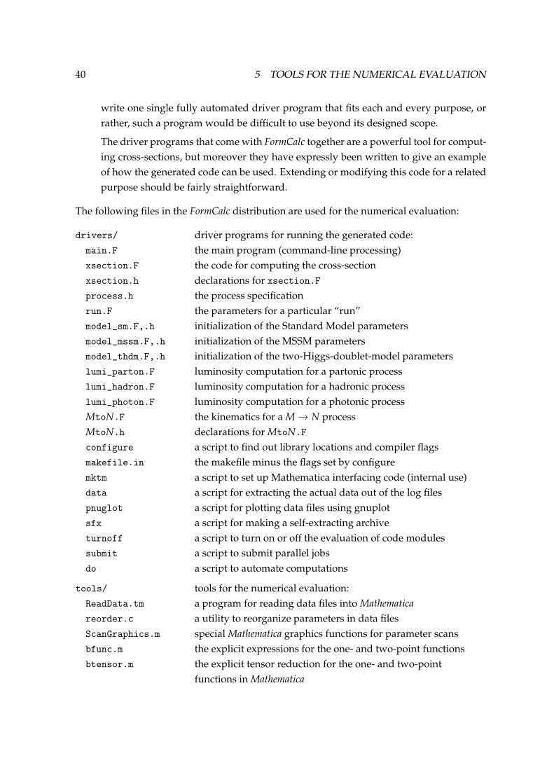
40 5 TOOLS FOR THE NUMERICAL EVALUATION
write one single fully automated driver program that fits each and every purpose, or
rather, such a program would be difficult to use beyond its designed scope.
The driver programs that come with FormCalc together are a powerful tool for comput-
ing cross-sections, but moreover they have expressly been written to give an example
of how the generated code can be used. Extending or modifying this code for a related
purpose should be fairly straightforward.
The following files in the FormCalc distribution are used for the numerical evaluation:
drivers/ driver programs for running the generated code:
main.F the main program (command-line processing)
xsection.F the code for computing the cross-section
xsection.h declarations for xsection.F
process.h the process specification
run.F the parameters for a particular “run”
model_sm.F,.h initialization of the Standard Model parameters
model_mssm.F,.h initialization of the MSSM parameters
model_thdm.F,.h initialization of the two-Higgs-doublet-model parameters
lumi_parton.F luminosity computation for a partonic process
lumi_hadron.F luminosity computation for a hadronic process
lumi_photon.F luminosity computation for a photonic process
MtoN.F the kinematics for a M → N process
MtoN.h declarations for MtoN.F
configure a script to find out library locations and compiler flags
makefile.in the makefile minus the flags set by configure
mktm a script to set up Mathematica interfacing code (internal use)
data a script for extracting the actual data out of the log files
pnuglot a script for plotting data files using gnuplot
sfx a script for making a self-extracting archive
turnoff a script to turn on or off the evaluation of code modules
submit a script to submit parallel jobs
do a script to automate computations
tools/ tools for the numerical evaluation:
ReadData.tm a program for reading data files into Mathematica
reorder.c a utility to reorganize parameters in data files
ScanGraphics.m special Mathematica graphics functions for parameter scans
bfunc.m the explicit expressions for the one- and two-point functions
btensor.m the explicit tensor reduction for the one- and two-point
functions in Mathematica

5.1 Generating code 41
5.1 Generating code
In most cases, the numerical evaluation of an amplitude directly in Mathematica is too slow,
so the FormCalc results need to be converted to a Fortran or C program. The simplest way to
do this in Mathematica is something like FortranForm[result] >> file.f. Unfortunately,
this leaves a lot to be done manually.
FormCalc contains two much more sophisticated functions for generating code,
WriteSquaredME and WriteRenConst. The philosophy is that the user should not have to
modify the generated code. This eliminates the source of many errors, but of course goes
well beyond simple translation to code: the code has to be encapsulated (i.e. no loose ends
the user has to bother with), and all necessary subsidiary files, such as include files and a
makefile, have to be produced. Also, the code has to be chopped into pieces small enough
that the compiler will accept them.
Before using WriteSquaredME or WriteRenConst, a directory must be created for the code
and the driver programs copied into this directory. This is done with SetupCodeDir:
SetupCodeDir[dir] create a directory dir and install the driver programs
necessary to compile the generated code in this
directory
Note that SetupCodeDir never removes or overwrites the directory or the driver programs,
so a code directory, once created, stays put. The Drivers option can be used to load cus-
tomized driver programs from a local directory.
Option default value
Drivers "drivers" a directory containing customized
versions of the driver programs which
take precedence over the default ones in
$DriversDir
To illustrate the concept, consider generating code for a particular scattering process. The
first time, no customized drivers exist and hence FormCalc copies the default drivers into
the code directory. The user then modifies, say, process.h. To preserve the changes, he
copies the file to a local directory, e.g. drivers, and specifies this directory with the Drivers
option. Now even if the code directory is deleted, generating the code anew will recover
all modifications because the customized version of process.h in drivers supersedes the
default process.h in $DriversDir.
The function WriteSquaredME assumes that there is a tree-level amplitude Mtree and a one-
loop amplitude M1-loop and writes out a subroutine called SquaredME which computes the
two expressions |Mtree|2 and 2 Re M∗treeM1-loop. When there is no tree-level contribution, 0

42 5 TOOLS FOR THE NUMERICAL EVALUATION
and |M1-loop|2 are returned, and when there is no one-loop contribution, |Mtree|2 and 0 are
returned.
WriteSquaredME[tree, loop,mat, abbr, . . . , dir]
generate code for a subroutine SquaredME in the
directory dir; this subroutine computes the squared
matrix element composed of the amplitudes tree (for
the tree-level part) and loop (for the one-loop part)
The tree and loop arguments are results of CalcFeynAmp and are trailed by all other objects
necessary for the computation of the squared matrix element, like helicity matrix elements,
colour matrix elements, and the abbreviations. An empty list, , is used to indicate that the
tree or loop argument is missing. Since WriteSquaredME has a rather complicated invocation,
it is perhaps best to give an example:
born = CalcFeynAmp[bornamps];
self = CalcFeynAmp[selfamps];
vert = CalcFeynAmp[vertamps];
box = CalcFeynAmp[boxamps];
col = ColourME[All, born];
dir = SetupCodeDir["fortran"];
WriteSquaredME[born, self, vert, box, col, Abbr[], dir]
The tree and loop arguments of WriteSquaredME have the somewhat unorthodox feature that
the naming of the code modules depends on the variable names chosen for the components
of the amplitude (like born, self, etc., in the example above). That is, WriteSquaredME tries
to name the code modules like the variables, e.g. the amplitude contained in the variable
self will be written to files of the form self*.F. This is only possible if the variable names
are plain symbols; in all other cases, the modules are named Tree1.F, Tree2.F, or Loop1.F,
Loop2.F, etc.
The following options can be used with WriteSquaredME.
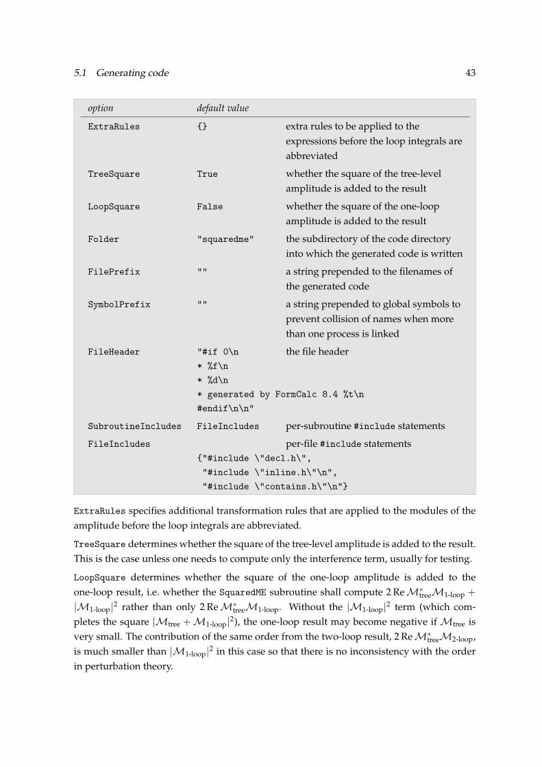
5.1 Generating code 43
option default value
ExtraRules extra rules to be applied to the
expressions before the loop integrals are
abbreviated
TreeSquare True whether the square of the tree-level
amplitude is added to the result
LoopSquare False whether the square of the one-loop
amplitude is added to the result
Folder "squaredme" the subdirectory of the code directory
into which the generated code is written
FilePrefix "" a string prepended to the filenames of
the generated code
SymbolPrefix "" a string prepended to global symbols to
prevent collision of names when more
than one process is linked
FileHeader "#if 0\n the file header
* %f\n
* %d\n
* generated by FormCalc 8.4 %t\n
#endif\n\n"
SubroutineIncludes FileIncludes per-subroutine #include statements
FileIncludes per-file #include statements
"#include \"decl.h\",
"#include \"inline.h\"\n",
"#include \"contains.h\"\n"
ExtraRules specifies additional transformation rules that are applied to the modules of the
amplitude before the loop integrals are abbreviated.
TreeSquare determines whether the square of the tree-level amplitude is added to the result.
This is the case unless one needs to compute only the interference term, usually for testing.
LoopSquare determines whether the square of the one-loop amplitude is added to the
one-loop result, i.e. whether the SquaredME subroutine shall compute 2 Re M∗treeM1-loop +
|M1-loop|2 rather than only 2 Re M∗treeM1-loop. Without the |M1-loop|2 term (which com-
pletes the square |Mtree +M1-loop|2), the one-loop result may become negative if Mtree is
very small. The contribution of the same order from the two-loop result, 2 Re M∗treeM2-loop,
is much smaller than |M1-loop|2 in this case so that there is no inconsistency with the order
in perturbation theory.
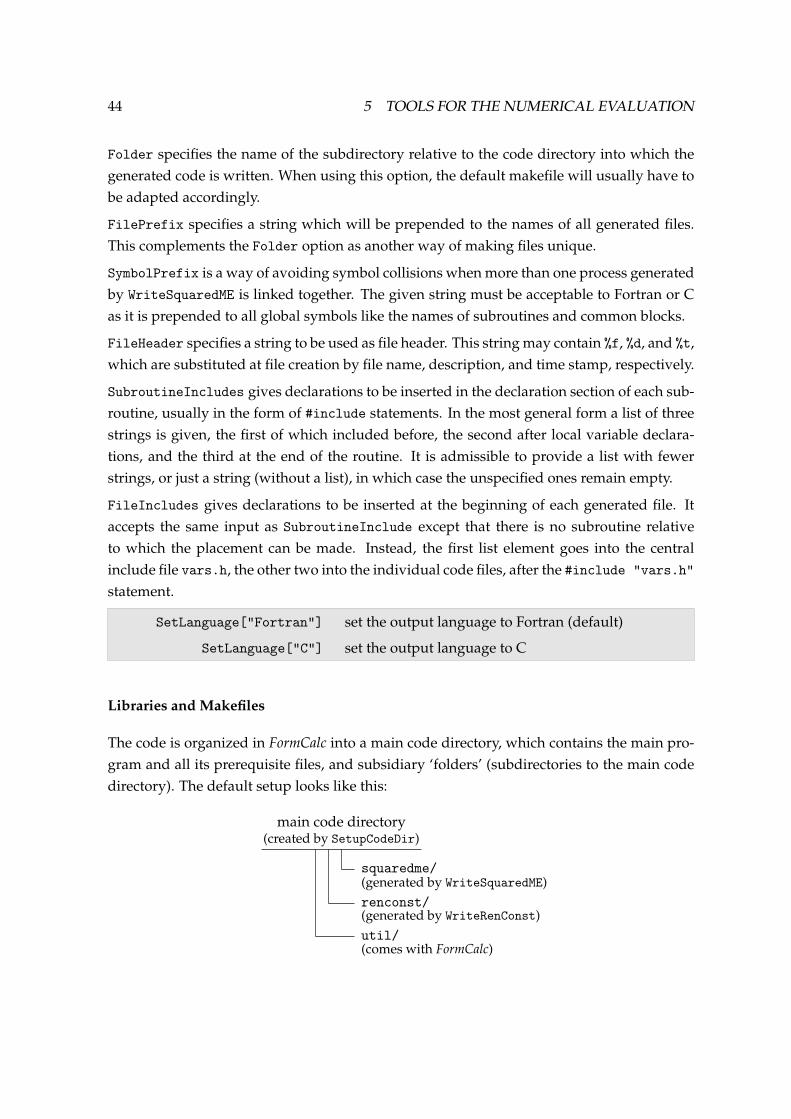
44 5 TOOLS FOR THE NUMERICAL EVALUATION
Folder specifies the name of the subdirectory relative to the code directory into which the
generated code is written. When using this option, the default makefile will usually have to
be adapted accordingly.
FilePrefix specifies a string which will be prepended to the names of all generated files.
This complements the Folder option as another way of making files unique.
SymbolPrefix is a way of avoiding symbol collisions when more than one process generated
by WriteSquaredME is linked together. The given string must be acceptable to Fortran or C
as it is prepended to all global symbols like the names of subroutines and common blocks.
FileHeader specifies a string to be used as file header. This string may contain %f, %d, and %t,
which are substituted at file creation by file name, description, and time stamp, respectively.
SubroutineIncludes gives declarations to be inserted in the declaration section of each sub-
routine, usually in the form of #include statements. In the most general form a list of three
strings is given, the first of which included before, the second after local variable declara-
tions, and the third at the end of the routine. It is admissible to provide a list with fewer
strings, or just a string (without a list), in which case the unspecified ones remain empty.
FileIncludes gives declarations to be inserted at the beginning of each generated file. It
accepts the same input as SubroutineInclude except that there is no subroutine relative
to which the placement can be made. Instead, the first list element goes into the central
include file vars.h, the other two into the individual code files, after the #include "vars.h"
statement.
SetLanguage["Fortran"] set the output language to Fortran (default)
SetLanguage["C"] set the output language to C
Libraries and Makefiles
The code is organized in FormCalc into a main code directory, which contains the main pro-
gram and all its prerequisite files, and subsidiary ‘folders’ (subdirectories to the main code
directory). The default setup looks like this:
main code directory(created by SetupCodeDir)
squaredme/(generated by WriteSquaredME)
renconst/(generated by WriteRenConst)
util/(comes with FormCalc)

5.1 Generating code 45
Each folder is equipped with its own makefile which makes a library of the same name, e.g.
the makefile in util/ makes the library util.a.
These sub-makefiles are orchestrated by the master makefile. Libraries required for the
main program are listed in the LIBS variable and built automatically by invoking the sub-
makefiles:
LIBS = squaredme.a renconst.a util.a
The master makefile is no longer overwritten in the code-generation process and is treated
like the other driver programs, i.e. a customized copy can be saved in the local drivers direc-
tory.
Occasionally it is useful to have more than one instance of squaredme (or renconst), e.g.
when computing an hadronic cross-section to which several partonic processes contribute.
Both WriteSquaredME and WriteRenConst have the Folder option, with which a unique
folder name can be chosen, and the SymbolPrefix option, with which the symbols visible to
the linker can be prefixed with a unique identifier. This identifier is inserted only at compile
time and can easily be changed in the sub-makefile at any time.
The util library is a collection of ancillary routines which currently includes:
• System utilities (log file management),
• Kinematic functions (Pair, Eps, . . . ),
• Diagonalization routines (DIAG library [Ha06]),
• Univariate integrators (Gauss, Patterson),
• Multivariate integrators (CUBA library [Ha04]).
Older versions of FormCalc used to include these directly into the main program. The library
version has the advantage that the linker selects only the routines that are actually needed,
and furthermore it is straightforward to add new code. The util.a library is compiled
once when FormCalc is installed and then copied to the main code directory, thus avoiding
unnecessary compiles.
Specifying numerical parameters
Numerical parameters are specified in the model initialization file, e.g. model_sm.F, with
declarations in model_sm.h. Each such initialization file must implement the following three
subroutines:
subroutine ModelDefaults

46 5 TOOLS FOR THE NUMERICAL EVALUATION
sets all model parameters to their initial values. This subroutine is invoked before the user
gets to set the input parameters.
subroutine ModelConstIni(fail)
integer fail
initializes the constant model parameters, i.e. the ones that do not depend on√
s, the centre-
of-mass energy. If the routine determines that the input parameters yield unphysical or
otherwise unacceptable model parameters, it must return a non-zero value in fail.
subroutine ModelVarIni(fail, sqrtS)
integer fail
double precision sqrtS
is called after ModelConstIni to initialize the model parameters that depend on√
s, typically
αs and derived quantities. Finally, the
subroutine ModelDigest
is invoked to print a digest of the model parameters.
Note one detail: some model constants are declared in model_x.h with parameter state-
ments, i.e. as numerical constants. WriteSquaredME can optimize the generated code based
on the information which symbols are numerical constants to the compiler and which are
variables.
The trick is to move the numerical constants to the front of each product so that the compiler
can combine these constants into one number, thus reducing the number of multiplications at
run time. For example, if WriteSquaredME knows Alfa2 and SW2 to be numerical constants,
it will write (3*Alfa2)/(8.D0*SW2**2)*(Abb1*cint44*MH2) instead of Mathematica’s de-
fault ordering (3*Abb1*Alfa2*cint44*MH2)/(8.D0*SW2**2). While this may seem a minor
rearrangement, the increase in execution speed can be 30%!
To tell WriteSquaredME which symbols are numerical constants to the compiler, simply as-
sign the symbol a numerical value like in (this statement is near the end of FormCalc.m)
Scan[ (N[#] = Random[])&, Alfa, Alfa2, MW, MW2, ... ]
Details of the code generation
The following excerpt is from a Fortran code generated by WriteSquaredME:
subroutine self

5.1 Generating code 47
implicit none
#include "vars.h"
Cloop(1) = Cloop(1) +
& ((3*Alfa2)/(8.D0*SW2**2)*(Abb1*cint44*MH2) +
& (9*Alfa2)/(8.D0*SW2**2)*(Abb1*cint5*MH2**2) +
& Alfa2/(4.D0*SW2**2)*(Abb1*cint41*(MH2 + 6*MW2)) +
& (Alfa2*MW2)/SW2**2*(Abb1*cint43*S) +
& (Alfa2*MW2)/(2.D0*CW2*SW2**2)*(Abb1*cint46*S) +
& Alfa2/(8.D0*CW2*SW2**2)*
& (Abb1*cint45*(6*MW2 + CW2*MH2)) ...
Note the use of the C preprocessor in statements like #include. Because of this, the code
files have the extension .F which is recognized by almost all Fortran compilers.
WriteSquaredME pulls the calculation of several kinds of objects out of the actual computa-
tion of the amplitude. That is, these objects are calculated first and stored in variables, and
then the amplitude is computed. Because the replacement of more complex objects by scalar
variables shortens the expressions, these objects are referred to as abbreviations.
The following objects are treated as abbreviations:
1. variables replacing some function call: Pairn (dot products), Epsn (contracted epsilon
tensors), cintn, iintn (loop integrals),
2. products or sums of variables of type 1: Abbn, AbbSumn,
3. matrix elements: MatType(i, j).
All of these abbreviations except the cintn and iintn are in fact the ones already introduced
by FormCalc. These abbreviations share the general feature of being costly in CPU time (in
particular the loop integrals), which means that for optimal performance they should be
calculated as few times as possible. WriteSquaredME splits them into 2 × 3 categories:
• abbr0_cat.F – tree-level, and
• abbr1_cat.F – one-loop,
• abbri_s.F – abbreviations which depend only on√
s,
• abbri_angle.F – abbreviations which depend also on other phase-space variables, but
not on the helicities, nad
• abbri_hel.F – helicity-dependent abbreviations.
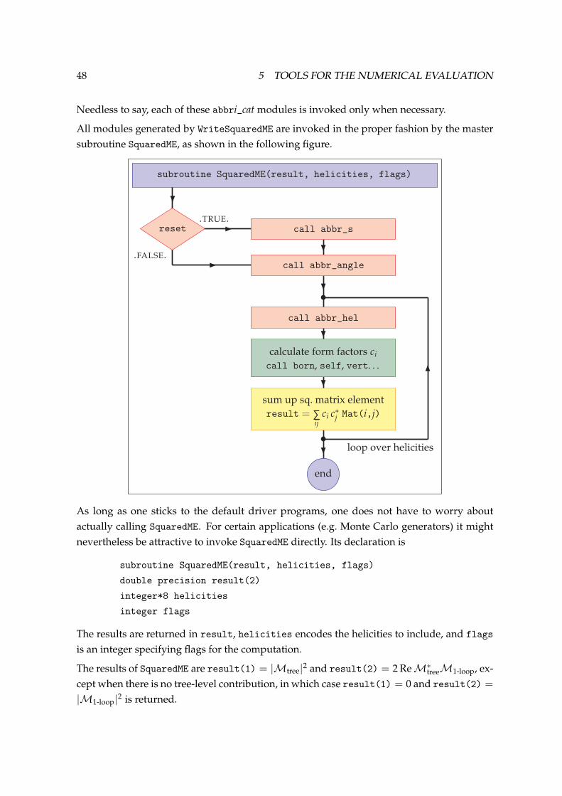
48 5 TOOLS FOR THE NUMERICAL EVALUATION
Needless to say, each of these abbri_cat modules is invoked only when necessary.
All modules generated by WriteSquaredME are invoked in the proper fashion by the master
subroutine SquaredME, as shown in the following figure.
.TRUE.
.FALSE.
reset
subroutine SquaredME(result, helicities, flags)
loop over helicities
call abbr_s
call abbr_angle
call abbr_hel
calculate form factors ci
call born, self, vert. . .
sum up sq. matrix element
result = ∑ij
ci c∗j Mat(i,j)
end
As long as one sticks to the default driver programs, one does not have to worry about
actually calling SquaredME. For certain applications (e.g. Monte Carlo generators) it might
nevertheless be attractive to invoke SquaredME directly. Its declaration is
subroutine SquaredME(result, helicities, flags)
double precision result(2)
integer*8 helicities
integer flags
The results are returned in result, helicities encodes the helicities to include, and flags
is an integer specifying flags for the computation.
The results of SquaredME are result(1) = |Mtree|2 and result(2) = 2 Re M∗treeM1-loop, ex-
cept when there is no tree-level contribution, in which case result(1) = 0 and result(2) =
|M1-loop|2 is returned.
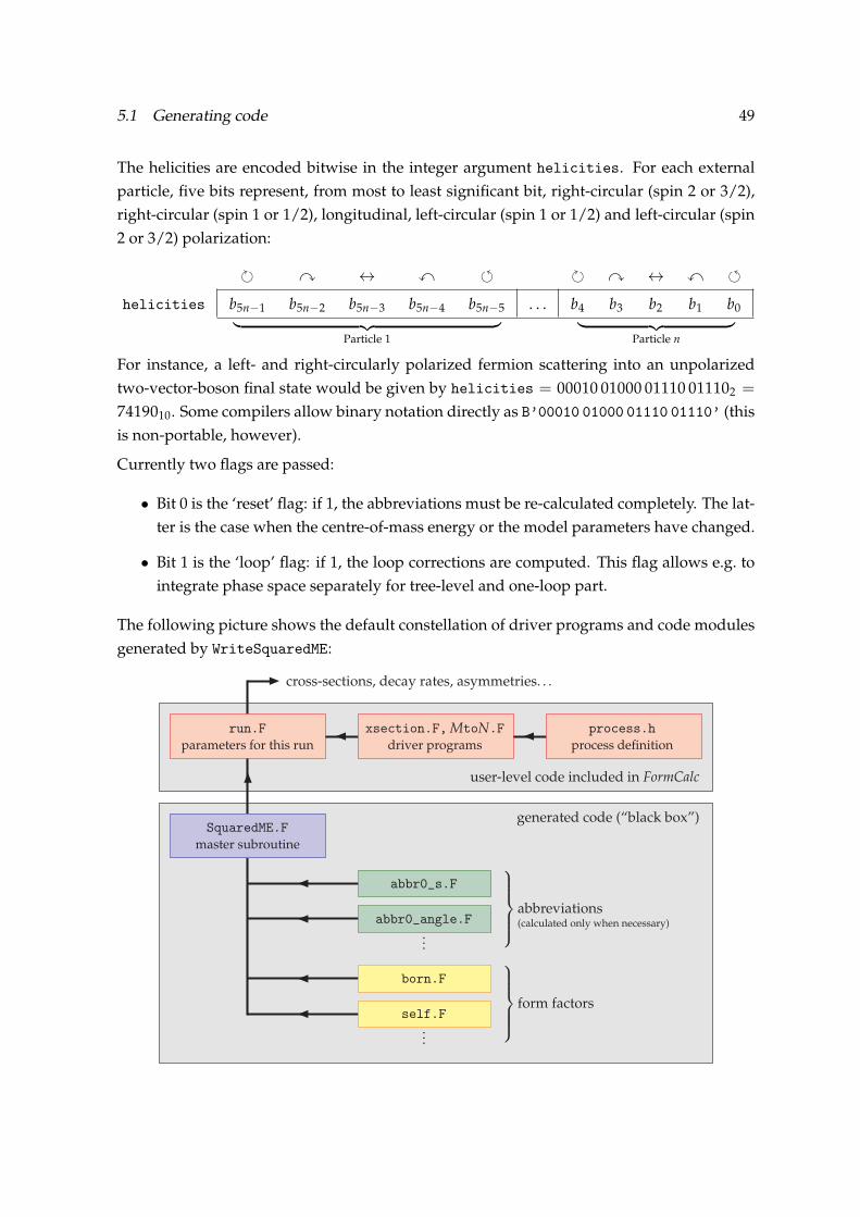
5.1 Generating code 49
The helicities are encoded bitwise in the integer argument helicities. For each external
particle, five bits represent, from most to least significant bit, right-circular (spin 2 or 3/2),
right-circular (spin 1 or 1/2), longitudinal, left-circular (spin 1 or 1/2) and left-circular (spin
2 or 3/2) polarization:
y ↔ x y ↔ x
helicities b5n−1 b5n−2 b5n−3 b5n−4 b5n−5 . . . b4 b3 b2 b1 b0
︸ ︷︷ ︸Particle 1
︸ ︷︷ ︸Particle n
For instance, a left- and right-circularly polarized fermion scattering into an unpolarized
two-vector-boson final state would be given by helicities = 00010 01000 01110 011102 =
7419010. Some compilers allow binary notation directly as B’00010 01000 01110 01110’ (this
is non-portable, however).
Currently two flags are passed:
• Bit 0 is the ‘reset’ flag: if 1, the abbreviations must be re-calculated completely. The lat-
ter is the case when the centre-of-mass energy or the model parameters have changed.
• Bit 1 is the ‘loop’ flag: if 1, the loop corrections are computed. This flag allows e.g. to
integrate phase space separately for tree-level and one-loop part.
The following picture shows the default constellation of driver programs and code modules
generated by WriteSquaredME:
user-level code included in FormCalc
generated code (“black box”)
cross-sections, decay rates, asymmetries. . .
SquaredME.F
master subroutine
abbr0_s.F
abbr0_angle.F
...
abbreviations(calculated only when necessary)
born.F
self.F
...
form factors
run.F
parameters for this run
xsection.F, MtoN.F
driver programs
process.h
process definition
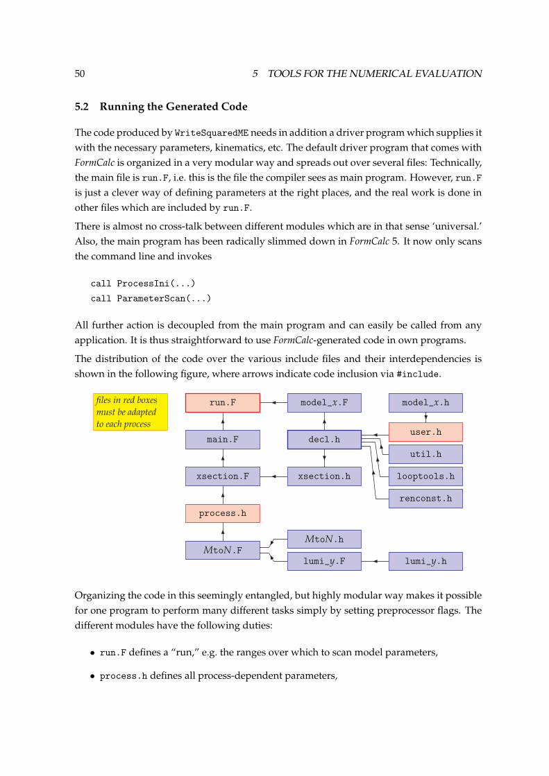
50 5 TOOLS FOR THE NUMERICAL EVALUATION
5.2 Running the Generated Code
The code produced by WriteSquaredME needs in addition a driver program which supplies it
with the necessary parameters, kinematics, etc. The default driver program that comes with
FormCalc is organized in a very modular way and spreads out over several files: Technically,
the main file is run.F, i.e. this is the file the compiler sees as main program. However, run.F
is just a clever way of defining parameters at the right places, and the real work is done in
other files which are included by run.F.
There is almost no cross-talk between different modules which are in that sense ‘universal.’
Also, the main program has been radically slimmed down in FormCalc 5. It now only scans
the command line and invokes
call ProcessIni(...)
call ParameterScan(...)
All further action is decoupled from the main program and can easily be called from any
application. It is thus straightforward to use FormCalc-generated code in own programs.
The distribution of the code over the various include files and their interdependencies is
shown in the following figure, where arrows indicate code inclusion via #include.
main.F
xsection.F
process.h
MtoN.F
xsection.h
model_x.F
user.h
util.h
looptools.h
renconst.h
MtoN.h
lumi_y.F
model_x.h
lumi_y.h
files in red boxes
must be adapted
to each process
run.F
decl.h
Organizing the code in this seemingly entangled, but highly modular way makes it possible
for one program to perform many different tasks simply by setting preprocessor flags. The
different modules have the following duties:
• run.F defines a “run,” e.g. the ranges over which to scan model parameters,
• process.h defines all process-dependent parameters,

5.2 Running the Generated Code 51
• main.F does the command-line parsing,
• xsection.F contains the kinematics-independent code,
xsection.h contains the declarations for xsection.F,
• MtoN.F contains the kinematics-dependent code for a M → N process,
MtoN.h contains the declarations for MtoN.F,
• model_x.F (currently one of model_sm.F, model_mssm.F, model_thdm.F) initializes the
model parameters,
model_x.h contains the declarations for model_x.F,
• lumi_y.F (currently one of lumi_parton.F, lumi_hadron.F, lumi_photon.F) calcu-
lates the parton luminosity,
lumi_y.h contains the declarations for lumi_y.F,
• util.h contains the declarations for the functions in the util library,
• looptools.h is the LoopTools include file,
• renconst.h declares the renormalization constants (see Sect. 5.4).
In this setup, the choice of parameters is directed by the two files process.h and run.F,
which include one each of
• Kinematics definitions:
1to2.F,
2to2.F,
2to3.F,
• Convolution with PDFs:
lumi_parton.F,
lumi_hadron.F,
lumi_photon.F,
• Model initialization:
model_sm.F,
model_mssm.F,
model_thdm.F.
5.2.1 Process definition
All process-specific definitions are given in process.h. The external particles are declared
in the lines

52 5 TOOLS FOR THE NUMERICAL EVALUATION
#define TYPEi ti
#define MASSi mi
#define CHARGEi ci
where each ti is one of the symbols SCALAR, FERMION, VECTOR, PHOTON, or GLUON. PHOTON is
the same as VECTOR except that longitudinal polarization states are not allowed and GLUON is
just an alias for PHOTON.
As in FormCalc, the momenta, masses, and polarization vectors are numbered sequentially
like in the following figure.
k1, m1, ε1
k2, m2, ε2
k3, m3, ε3
k4, m4, ε4...
In addition to the external particles, the following items are defined in process.h:
• a colour factor (COLOURFACTOR), to account for coloured particles in the initial state,
• a combinatorial factor (IDENTICALFACTOR), to account for identical particles in the final
state,
• a wave-function renormalization (WF_RENORMALIZATION), if a non-onshell renormaliza-
tion scheme is used,
• whether soft bremsstrahlung shall be added (BREMSSTRAHLUNG), and the maximum en-
ergy a soft photon may have (ESOFTMAX) (see Sect. 5.5 for details).
5.2.2 Building up phase space
FormCalc builds up the n-particle phase space iteratively by nested integrations over the
invariant mass Mi and solid angle Ωi of each outgoing particle i. This procedure is encoded
in the subroutine Split:

5.2 Running the Generated Code 53
call Split
√
sm1Ω1
M1
m2
Ω2
M2. . .
mn−1
Ωn−1
Ωn
mn
Counting the degrees of freedom, there are (n − 1) M-integrations and n Ω-integrations.
The corresponding phase-space parameterization is
1
2√
s
∫ √s−m1
m2+···+mn
dM1 dΩ1k1
2
×∫ M1−m2
m3+···+mn
dM2 dΩ2k2
2
× · · ·
×∫ Mn−2−mn−1
mn
dMn−1 dΩn−1kn−1
2
×∫
dΩnkn
2
where dΩi = d cosθi dϕi. The particle’s momentum ki and cosθi are given in the respective
decay’s rest frame. The ϕ1-integration is trivial because of axial symmetry. From the prac-
tical point of view this looks as follows (this code is taken almost verbatim from FormCalc’s
2to3.F):
p = 0
ex = 0
ey = 0
ez = 1
minv = sqrtS
msum = MASS3 + MASS4 + MASS5
call Split(5, dble(MASS5),
& p, ex,ey,ez, minv, msum, fac, 0,
& Var(XMREM5), Var(XCOSTH5), Var(TRIVIAL))
call Split(4, dble(MASS4),
& p, ex,ey,ez, minv, msum, fac, 0,
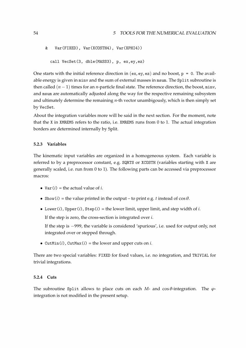
54 5 TOOLS FOR THE NUMERICAL EVALUATION
& Var(FIXED), Var(XCOSTH4), Var(XPHI4))
call VecSet(3, dble(MASS3), p, ex,ey,ez)
One starts with the initial reference direction in (ex, ey, ez) and no boost, p = 0. The avail-
able energy is given in minv and the sum of external masses in msum. The Split subroutine is
then called (n− 1) times for an n-particle final state. The reference direction, the boost, minv,
and msum are automatically adjusted along the way for the respective remaining subsystem
and ultimately determine the remaining n-th vector unambigously, which is then simply set
by VecSet.
About the integration variables more will be said in the next section. For the moment, note
that the X in XMREM5 refers to the ratio, i.e. XMREM5 runs from 0 to 1. The actual integration
borders are determined internally by Split.
5.2.3 Variables
The kinematic input variables are organized in a homogeneous system. Each variable is
referred to by a preprocessor constant, e.g. SQRTS or XCOSTH (variables starting with X are
generally scaled, i.e. run from 0 to 1). The following parts can be accessed via preprocessor
macros:
• Var(i) = the actual value of i.
• Show(i) = the value printed in the output – to print e.g. t instead of cosθ.
• Lower(i), Upper(i), Step(i) = the lower limit, upper limit, and step width of i.
If the step is zero, the cross-section is integrated over i.
If the step is −999, the variable is considered ‘spurious’, i.e. used for output only, not
integrated over or stepped through.
• CutMin(i), CutMax(i) = the lower and upper cuts on i.
There are two special variables: FIXED for fixed values, i.e. no integration, and TRIVIAL for
trivial integrations.
5.2.4 Cuts
The subroutine Split allows to place cuts on each M- and cosθ-integration. The ϕ-
integration is not modified in the present setup.

5.2 Running the Generated Code 55
Cuts restricting Mi Cuts restricting cosθi
Cut on Key Cut on Key
Mi CUT_MREM cosθi CUT_COSTH
Ei CUT_MREM_E cos θi CUT_COSTHCMS
ki CUT_MREM_K Ei CUT_COSTH_E
ET,i CUT_MREM_ET ki CUT_COSTH_K
kT,i CUT_MREM_KT
yi CUT_MREM_RAP
ηi CUT_MREM_PRAP
In practice, the application of cuts works as follows:
key = 0
CutMin(XMREM5) = E5MIN
key = key + Cut(CUT_MREM_E, CUT_MIN)
CutMin(XCOSTH5) = -(1 - COSTH5CUT)
CutMax(XCOSTH5) = +(1 - COSTH5CUT)
key = key + Cut(CUT_COSTH, CUT_MIN + CUT_MAX)
call Split(5, dble(MASS5),
& p, ex,ey,ez, minv, msum, fac, key,
& Var(XMREM5), Var(XCOSTH5), Var(TRIVIAL))
...
The value of the cut is deposited in CutMin or CutMax and the cut registered by adding an
identifier for the cut to the integer key, e.g. Cut(CUT_MREM_E, CUT_MIN) specifies a cut on
the energy (CUT_MREM_E) from below (CUT_MIN) which is used to restrict the invariant-mass
integration (CUT_MREM_E).
Note that these cuts really restrict the integration limits. They do not introduce veto func-
tions (1 in wanted, 0 in unwanted areas) into the integrand, which can severely hamper
convergence.
In addition, for each external particle i several kinematical quantities are available:
• momspec(SPEC_M,i) – mass m,
• momspec(SPEC_E,i) – energy E,

56 5 TOOLS FOR THE NUMERICAL EVALUATION
• momspec(SPEC_K,i) – momentum k,
• momspec(SPEC_ET,i) – transverse energy ET,
• momspec(SPEC_KT,i) – transverse momentum kT,
• momspec(SPEC_RAP,i) – rapidity y,
• momspec(SPEC_PRAP,i) – pseudo-rapidity η,
• momspec(SPEC_DELTAK,i) – the difference E − k.
5.2.5 Convolution
With the new variable system, the convolution with arbitrary parton distribution functions
can easily be achieved. Three modules are already included in FormCalc 5:
• lumi_parton.F = initial-state partons, no convolution.
• lumi_hadron.F = initial-state hadrons, convolution with hadronic PDFs from the
LHAPDF library [WhBG05].
• lumi_photon.F = initial-state photons, convolution with CompAZ spectrum [Za03].
5.2.6 Integration parameters
Depending on the integrand, the actual integration can be fairly tricky to carry out numeri-
cally. 2to3.F employs the CUBA library [Ha04] which offers four integration routines. The
CUBA parameters are chosen in run.F as preprocessor variables:
#define METHOD DIVONNE
#define RELACCURACY 1D-3
#define ABSACCURACY 1D-7
#define VERBOSE 1
#define MINEVAL 0
#define MAXEVAL 50000
* for Vegas:
#define NSTART 1000
#define NINCREASE 500
* for Suave:
#define NNEW 1000

5.2 Running the Generated Code 57
#define FLATNESS 50
* for Divonne:
#define KEY1 47
#define KEY2 1
#define KEY3 1
#define MAXPASS 5
#define BORDER 1D-6
#define MAXCHISQ 10
#define MINDEVIATION .25D0
* for Cuhre:
#define KEY 0
The integration algorithm is selected with METHOD, which can take the values VEGAS, SUAVE,
DIVONNE, and CUHRE. The other preprocessor variables determine parameters of the integra-
tors and may/should be tuned for a particular integrand, for details see [Ha04].
5.2.7 Compiling and running the code
The code produced by WriteSquaredME is compiled with the commands
./configure
make
The configure script searches for the compilers and necessary libraries and writes out a
makefile by adding the appropriate locations and flags to makefile.in. The ‘usual’ envi-
ronment variables like FC (Fortran compiler) and FFLAGS (Fortran flags) can be used to force
particular choices.
Based on the makefile, the make command then builds the executable. Its default name is
run, which is quite natural because the Fortran compiler sees run.F as the main program, as
mentioned before. The advantage is that for a different run, one can make a copy of run.F,
say run1.F, with different parameters. This new run is compiled with “make run1” and
results in the executable run1. Thus, one can have several executables for different runs in
one directory.
The way the makefile compiles the code is also convenient if one wants to use the generated
subroutine SquaredME alone, i.e. without the surrounding driver programs. The necessary
object files are all placed in the library squaredme.a so that only a single file needs to be
linked. It is possible to build just this library with

58 5 TOOLS FOR THE NUMERICAL EVALUATION
make squaredme.a
The executables (run, run1, etc.) are able to calculate differential and integrated cross-
sections for particles of arbitrary polarization depending on the command line.
run p1 . . . pn sqrtS [serialfrom[,serialto[,serialstep]]]
compute the differential cross-section at a
centre-of-mass energy sqrtS with the external
particles polarized according to p1 . . . pn.
run p1 . . . pn sqrtSfrom,sqrtSto[,sqrtSstep] [serialfrom[,serialto[,serialstep]]]
compute the integrated cross-section in the energy
range sqrtSfrom–sqrtSto in steps of sqrtSstep, p1 . . . pn
being the polarizations of the external particles.
The pi can take the following values:
u for an unpolarized particle,
t for a transversely polarized particle,
+ for right-circular polarization,
- for left-circular polarization, and
0 for longitudinal polarization.
For a scalar particle, the polarization parameter must be present on the command line al-
though its value is ignored. The energies are specified in GeV. If an energy is below thresh-
old, run issues a warning and sets the energy to the threshold + 0.01 GeV.
A serial number range may optionally be added as a third argument, restricting the param-
eter scans. This is normally used only internally by the submit script (see below).
Important: If a particular polarization was already fixed during the algebraic simplification,
e.g. if _Hel = 0 was set in FormCalc to calculate with unpolarized external fermions, the
code thus produced can never compute a cross-section for a different polarization, no mat-
ter how the executable is invoked. Running such code with an incompatible polarization
will in general only result in a wrong averaging factor.
5.2.8 Parallelization and Vectorization
The assembly of the squared matrix element in code generated by FormCalc can be sketched
as in the following figure, where the helicity loop sits at the center of the calculation:

5.2 Running the Generated Code 59
Loop(s) over√
s & model parameters
Loop(s) over angular variables
Loop over helicities λ1, . . . , λn
σ += ∑c Cc M0c (λ1, . . . , λn)∗
M1c (λ1, . . . , λn)
The helicity loop is not only strategically the most desirable but also the most obvious candi-
date for concurrent execution. FormCalc can distribute the helicity loop in two ways: paral-
lel execution via fork/wait on the cores of the local CPU (i.e. SMP), and vectorization using
the CPU’s SIMD instructions (that is, the squared matrix element is computed for several
helicity combinations at once), or both. The include file distrib.h chooses the distribution
properties of the compiled code. Distribution of scans over parameter space is described in
Sect. 5.2.9.
Parallel execution with fork/wait is switched on by setting the preprocessor variable
PARALLEL in distrib.h to 1. The drawback of this method is that it competes for compute
cores in particular with Cuba. In the usual settings of few (e.g. 4 or 8) cores per system the
cores should be assigned to Cuba since it computes entire phase-space points in parallel,
not just the helicity loop. The number of cores is determined from the environment variable
FCCORES, or if that is not set, from the number of cores reported by the system minus the
current load average.
Vectorization is turned on automatically by the configure script if it detects that the CPU and
compiler are capable of it. If this is in conflict with plans to send the executable on a cluster
of computers with heterogeneous SIMD capabilities, run configure with the --generic op-
tion. Then again, SIMD instructions are typically available on recent computers: SSE3 since
2004, AVX since 2011. To control vectorization ‘by hand’ one needs to specify the preproces-
sor variable SIMD in distrib.h rather than including the file simd.h generated by configure.
SIMD specifies the length of the vector, sensible values are 2 for AVX, 1 for SSE3, and 0 other-
wise. In Fortran the vector length can in principle been chosen arbitrarily though a speedup
is expected only for the mentioned values commensurate with the hardware.
On top of this, the calculation automatically detects and omits helicity combinations con-
tributing negligibly. This feature is controlled by the two environment variables FCHSELN
and FCHSELEPS in the following way: for the first FCHSELN phase-space points, the compu-
tation runs over all helicity combinations h and the absolute value of the squared matrix
element is added up in an array t(h). For subsequent phase-space points, then, only helicity
combinations with a t-value larger than(FCHSELEPS ·maxh t(h)
)are actually computed. Un-
less one intentionally begins sampling e.g. on the borders of phase-space, the default values

60 5 TOOLS FOR THE NUMERICAL EVALUATION
FCHSELN = 10 and FCHSELEPS = 10−7 should be sufficient. In case of doubt about the valid-
ity of the result, the value of FCHSELN should be increased, or set to zero (which turns the
detection off).
If algebraic relations between helicities are known from analytic considerations, these can
be specified in Mathematica before calling WriteSquaredME and will restrict the sum over
helicities accordingly. For example:
Hel[2] = -Hel[1];
WriteSquaredME[...]
5.2.9 Scans over parameter space
To perform a scan, the actual calculation needs to be enclosed in a number of do-loops in
which the values of the scanned parameters are changed, i.e. a structure of the form
do 1 para1 = . . .
do 1 para2 = . . . etc.
calculate the cross-section
1 continue
run.F provides several preprocessor variables, LOOP1. . . LOOP15, which may be defined to
contain the do-statements that initiate the loops. Each loop must terminate on statement 1,
just as above. For example, the lines
#define LOOP1 do 1 MT = 160, 180, 5
#define LOOP2 do 1 MH = 100, 300, 100
result in a scan of the form
do 1 MT = 160, 180, 5
do 1 MH = 100, 300, 100
calculate the cross-section
1 continue
The loops are nested inside each other with LOOP1 being the outermost loop. It is not manda-
tory to declare a loop with each LOOPn, also a fixed value may be given as in the following
definition:
#define LOOP1 MH = 115
When scanning over parameter space, it is further necessary to keep track of the parameter
values for each data set. This is done by defining PRINT commands in the preprocessor
5.2 Running the Generated Code 61
variables PRINT1. . . PRINT5 in run.F. The PRINT command takes pairs of arguments, first a
string identifying the variable and then the variable itself. Defining, for example,
#define PRINT1 PRINT "MT=", MT, "MH=", MH
causes each data set to be preceded by two lines of the form
# MT= 160.00
# MH= 100.00
Such a scan can be a real CPU hog, but on the other hand, the calculation can be performed
completely independently for each parameter set and is thus an ideal candidate for par-
allelization. The real question is thus not how to parallelize the calculation, but how to
automate the parallelization.
The obstacle to automatic parallelization is that the loops are user-defined and in general
nested. A serial number is introduced to unroll the loops:
serial = 0
LOOP1
LOOP2...
serial = serial + 1
if( serial not in allowed range ) goto 1
calculate cross-section
1 continue
As mentioned before, the serial number range can be specified on the command line so that it
is quite straightforward to distribute patches of serial numbers on different machines. Most
easily this is done in an interleaved manner, since one then does not need to know to which
upper limit the serial number runs, i.e. if there are N machines available, send serial numbers
1, N + 1, 2N + 1, . . . on machine 1, send serial numbers 2, N + 2, 2N + 2, . . . on machine 2,
etc.
This procedure is automated in FormCalc: The user once creates a .submitrc file in his home
directory and lists there all machines that may be used, one on each line. The only require-
ment is that the machines are binary compatible because the same executable will be started
on each. In the case of multi-processor machines the number of processors is given after the
host name. Empty lines and lines beginning with # are treated as comments. Furthermore,
a line of the form nice n determines the nice value at which the remote jobs are started. For
example:
# .submitrc for FormCalc for the institute cluster
62 5 TOOLS FOR THE NUMERICAL EVALUATION
# start jobs with nice 10:
nice 10
pcxeon1 8
pcxeon2 8
pcjoe
pcath6
pcath7
The executable compiled from FormCalc code, typically called run, is then simply prefixed
with submit. For instance, instead of
run uuuu 500,1000
the user invokes
submit run uuuu 500,1000
The submit script uses ruptime to determine the load of the machines and ssh to log in.
Handling of the serial number is invisible to the user.
5.2.10 Log files, Data files, and Resume
Due to the parallelization mechanism, a single output file is not sufficient. Instead, FormCalc
creates a directory for each invocation of run, e.g. run.UUUU.00200 for a differential cross-
section or run.UUUU.00200-00500:00010 for an integrated cross-section (where 00010 is the
step width in the loop over the energy), opens one log file for each serial number in this
directory, and redirects console output to this file.
Each log file contains both the ‘real’ data and the ‘chatter’ (progress, warning, and error mes-
sages). This has the advantage that no unit numbers must be passed between subroutines
– every bit of output is simply written to the console (unit * in Fortran). It also makes it
easier to pinpoint errors, since the error message appears right next to the corrupted data.
The ‘real’ data are marked by a “|” in column 1 and there exists a simple shell script, data,
to extract the real data from the log file. For example,
data run.UUUU.00200
creates a data file run.UUUU.00200.data containing only the ‘real’ data arranged in three
columns, where the first column is the scattering angle in radians, the second column is the
tree-level cross-section, and the third column is the one-loop correction. For an integrated
5.2 Running the Generated Code 63
cross-section, there are five columns:√
s, the tree-level cross-section, the one-loop correction,
and the integration errors for the tree-level and one-loop cross-sections. Cross-sections are
computed in picobarn.
The log-file management also provides an easy way to resume an aborted calculation. This
works as follows: when running through the loops of a parameter scan, the log file for a
particular serial number
• may not exist: then it is created with execute permissions,
• may exist, but have execute permissions: then it is overwritten,
• may exist and have read-write permissions: then this serial number is skipped.
The execute permissions, which serve here merely as a flag to indicate an ongoing calcula-
tion, are reduced to ordinary read-write permissions when the log file is closed.
In other words, the program skips over the parts of the calculation that are already finished,
so all the user has to do to resume an aborted calculation is start the program again with the
same parameters.
5.2.11 Shell scripts
turnoff switches off (and on) the evaluation of certain parts of the amplitude, which is a
handy thing for testing. For example, “./turnoff box” switches off all parts of the ampli-
tude with ‘box’ in their name. Invoking turnoff without any argument restores all modules.
sfx packs all source files (but not object, executable, or log files) in the directory it is invoked
in into a mail-safe self-extracting archive. For example, if sfx is invoked in the directory
myprocess, it produces myprocess.sfx. This file can e.g. be mailed to a collaborator, who
needs to say “./myprocess.sfx x” to unpack the contents.
pnuglot produces a high-quality plot in Encapsulated PostScript format from a data file in
just one line. In fact, pnuglot does not even make the plot itself, it writes out a shell script to
do that, thus “./pnuglot mydata” creates mydata.gpl which then runs gnuplot, LATEX, and
dvips to create mydata.eps. The advantage of this indirect method is that the default gnuplot
commands in mydata.gpl can subsequently be edited to suit the user’s taste. Adding a label
or choosing a different line width is, for example, a pretty trivial matter. Needless to say, all
labels are in LATEX and Type 1 fonts are selected to make the EPS file nicely scalable.
pnuglot by default uses commands only available in gnuplot version 3.7 or higher. This
version can be obtained from http://www.gnuplot.info.

64 5 TOOLS FOR THE NUMERICAL EVALUATION
pnuglot [opts] file1 file2 . . . make a plot of the data files file1, file2, . . .
options:
-o outfile how to name the output file: the plotting script will
be called outfile.gpl and the actual plot outfile.eps.
The default is outfile = file1.
-2 use only columns 1:2 (usually the tree-level
cross-section) for plotting
-3 use only columns 1:(2+3) (usually the one-loop
corrected cross-section) for plotting
5.3 The Mathematica Interface
The Mathematica interface turns the stand-alone code into a Mathematica function for eval-
uating the cross-section or decay rate as a function of user-selected model parameters. The
benefits of such a function are obvious, as the whole instrumentarium of Mathematica com-
mands can be applied to them. For example, it is quite straightforward, using Mathematica’s
FindMinimum, to determine the minimum (or maximum) of the cross-section over a piece of
parameter space.
Interfacing is done using the MathLink protocol. The changes necessary to produce a Math-
Link executable are quite superficial and affect only the file run.F, where the user has to
choose which model parameters are interfaced from Mathematica.
To make the obvious even clearer, the cross-section is not evaluated in Mathematica, but in
Fortran or C, and only the numerical results are transferred back to Mathematica. One thing
one cannot do thus is to increase the numerical precision of the calculation using Mathemat-
ica commands like SetPrecision.
5.3.1 Setting up the Interface
The model parameters are specified in the file run.F. Typical definitions for stand-alone
code look like (here from an MSSM calculation with TB = tanβ and MA0 = MA0):
#define LOOP1 do 1 TB = 5, 50, 5
#define LOOP2 MA0 = 500
...
These lines declare TB to be scanned from 5 to 50 in steps of 5 and set MA0 to 500 GeV. To be
able to specify TB in Mathematica instead, the only change is

5.3 The Mathematica Interface 65
#define LOOP1 call MmaGetReal(TB)
Such invocations of MmaGetReal and its companion subroutines serve two purposes. At
compile time they determine with which arguments the Mathematica function is generated
(for details see below), and at run time they actually transfer the function’s arguments to the
specified variables.
MmaGetInteger(i) read the integer/real/complex parameter i/r/c
MmaGetReal(r) from Mathematica
MmaGetComplex(c)
MmaGetIntegerList(i, n) read the integer/real/complex parameter list i/r/c
MmaGetRealList(r, n) of length n from Mathematica
MmaGetComplexList(c, n)
Note that without a separate MmaGetReal call, MA0 would still be fixed by the Fortran state-
ment, i.e. not be accessible from Mathematica.
Once the makefile detects the presence of these subroutines, it automatically generates inter-
facing code and compiles a MathLink executable. For a file run.F the corresponding Math-
Link executable is also called run, as in the stand-alone case. This file is not started from the
command-line, but used in Mathematica as
Install["run"]
5.3.2 The Interface Function in Mathematica
After loading the MathLink executable with Install, a Mathematica function of the same
name is available. For definiteness, we will call this function ‘run’ in the following since
‘run.F’ is the default parameter file. This function has the arguments
run[sqrtS, arg1, arg2, ..., options]
run[sqrtSfrom, sqrtSto[, sqrtSstep], arg1, arg2, ..., options]
The first form computes a differential cross-section at√
s = sqrtS. The second form computes
a total cross-section for energies√
s varying from sqrtSfrom to sqrtSto in steps of sqrtSstep.
This is in one-to-one correspondence with the command-line invocation of the stand-alone
executable.
The arg1, arg2, . . . , are the model parameters declared automatically by the presence of their
MmaGetReal,Complex calls (see above). They appear in the argument list in the same order
as the corresponding MmaGetReal,Complex calls.
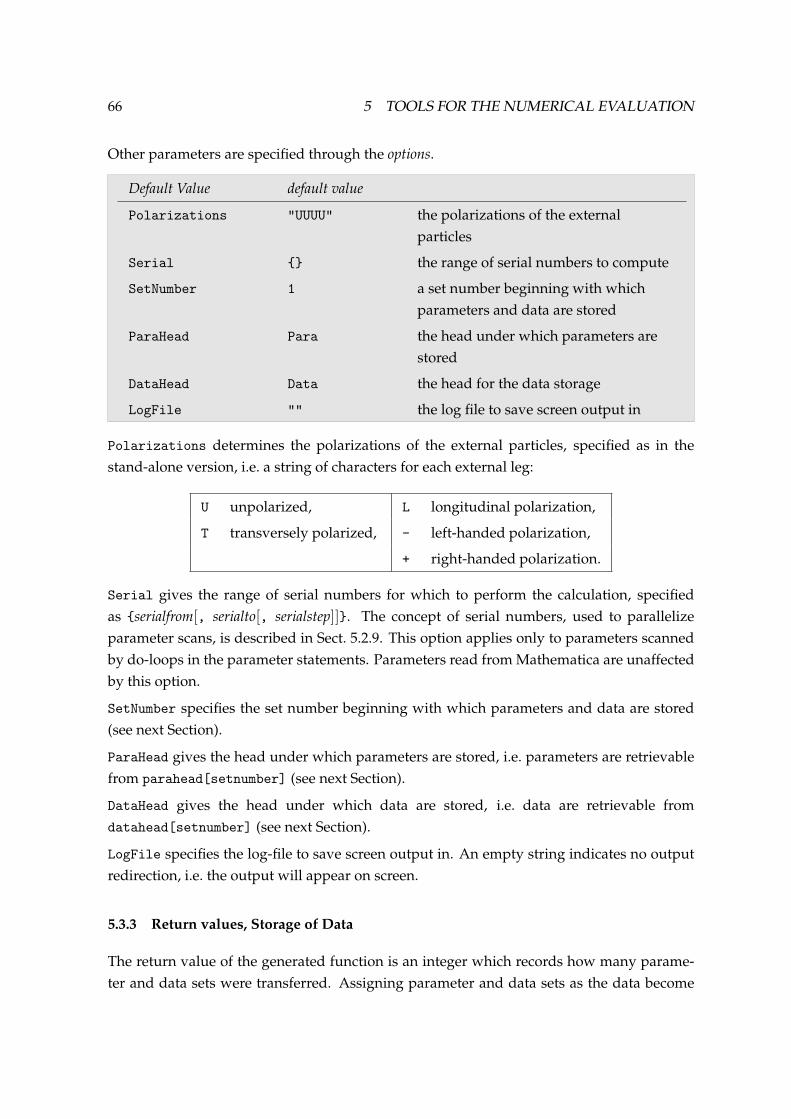
66 5 TOOLS FOR THE NUMERICAL EVALUATION
Other parameters are specified through the options.
Default Value default value
Polarizations "UUUU" the polarizations of the external
particles
Serial the range of serial numbers to compute
SetNumber 1 a set number beginning with which
parameters and data are stored
ParaHead Para the head under which parameters are
stored
DataHead Data the head for the data storage
LogFile "" the log file to save screen output in
Polarizations determines the polarizations of the external particles, specified as in the
stand-alone version, i.e. a string of characters for each external leg:
U unpolarized, L longitudinal polarization,
T transversely polarized, - left-handed polarization,
+ right-handed polarization.
Serial gives the range of serial numbers for which to perform the calculation, specified
as serialfrom[, serialto[, serialstep]]. The concept of serial numbers, used to parallelize
parameter scans, is described in Sect. 5.2.9. This option applies only to parameters scanned
by do-loops in the parameter statements. Parameters read from Mathematica are unaffected
by this option.
SetNumber specifies the set number beginning with which parameters and data are stored
(see next Section).
ParaHead gives the head under which parameters are stored, i.e. parameters are retrievable
from parahead[setnumber] (see next Section).
DataHead gives the head under which data are stored, i.e. data are retrievable from
datahead[setnumber] (see next Section).
LogFile specifies the log-file to save screen output in. An empty string indicates no output
redirection, i.e. the output will appear on screen.
5.3.3 Return values, Storage of Data
The return value of the generated function is an integer which records how many parame-
ter and data sets were transferred. Assigning parameter and data sets as the data become

5.3 The Mathematica Interface 67
available has several advantages:
• the return value of run is an integer rather than a large, bulky list,
• the parameters corresponding to a particular data set are easy to identify, e.g.
Para[4711] contains the parameters corresponding to Data[4711],
• most importantly, if the calculation is prematurely aborted, the parameters and data
transferred so far are still accessible.
Both, the starting set number and the heads of the parameter and data assignments can be
chosen with the options SetNumber, ParaHead, and DataHead, respectively.
The parameters which are actually returned are chosen by the user in the PRINTn statements
in run.F in much the same way as parameters are selected for printout in the stand-alone
code. To specify that TB and MA0 be returned, one needs the definitions
#define PRINT1 call MmaPutReal("TB", TB)
#define PRINT2 call MmaPutReal("MA0", MA0)
Notwithstanding, parameters can still be printed out, in which case they end up in the log
file (or on screen, if no log file is chosen). To transfer e.g. TB to Mathematica and print it out,
one would use
#define PRINT1 call MmaPutReal("TB", TB)
#define PRINT2 SHOW "TB", TB
An analogous subroutine exists of course for integer and complex parameters, too.
MmaPutInteger(s, i) transfer the integer/real/complex parameter i/r/c
MmaPutReal(s, r) to Mathematica under the name s
MmaPutComplex(s, c)
MmaPutIntegerList(s, i, n) transfer the integer/real/complex parameter list
MmaPutRealList(s, r, n) i/r/c of length n to Mathematica under the name s
MmaPutComplexList(s, c, n)
The parameters are stored in the form of rules in Mathematica, i.e. as name -> value. The first
argument specifies the left-hand side of this rule. It need not be a symbol in the strict sense,
but can be an arbitrary Mathematica expression. But note that in particular the underscore
has a special meaning in Mathematica and may not be used in symbol names. The second
argument is then the right-hand side of the rule and can be an arbitrary Fortran expression
containing model parameters, kinematic variables, etc.

68 5 TOOLS FOR THE NUMERICAL EVALUATION
The following example demonstrates the form of the parameter and data assignments.
Shown are results of a differential cross-section for a 2 → 2 reaction at one point in MSSM
parameter space. Within the data the varied parameter is cosθ, the scattering angle.
Para[1] = TB -> 1.5, MUE -> -1000., MSusy -> 1000.,
MA0 -> 700., M2 -> 100.
Data[1] = DataRow[500., -0.99,
0.10592302458950732, 0.016577997941111422,
0., 0.],
DataRow[500., -0.33,
0.16495552191438356, 0.014989931149150608,
0., 0.],
DataRow[500., 0.33,
0.2986891221231292, 0.015013326141014818,
0., 0.],
DataRow[500., 0.99,
0.5071238252157443, 0.012260927614082411,
0., 0.]
DataRow[v, r, e] a row of data with kinematic variables v,
cross-section or decay-rate results r, and integration
error e
The DataRow[v, r, e] function has three arguments:
• the unintegrated kinematic variables (v = √s, cosθ above),
• the cross-section or decay-rate results (r = tree-level result, one-loop correctionabove), and
• the respective integration errors (e = 0, 0 above, as this example originates from the
computation of a differential cross-section where no integration is performed).
5.3.4 Using the Generated Mathematica Function
To the Mathematica novice it may not be obvious how to use the function described above
to analyse data, produce plots, etc.
As an example, let us produce a contour plot of the cross-section in the MA0–tanβ plane. It
is assumed that the function run has the two parameters MA0 and TB in its argument list:

5.4 Renormalization Constants 69
Install["run"]
xs[sqrtS_, MA0_, TB_] := (
run[sqrtS, sqrtS, MA0, TB];
Data[1][[1, 2]] )
ContourPlot[xs[500, MA0, TB], MA0, 100, 500, TB, 5, 50]
The function xs runs the code and selects the data to plot. The first argument of run,
sqrtS, sqrtS, instructs the code to compute the total cross-section for just one point in
energy. We then select the first (and only) DataRow in the output and choose its second argu-
ment, the cross-section results: Data[1][[1, 2]].
This example can be extended a little to produce a one-dimensional plot where e.g. for
each value of tanβ the minimum and maximum of the cross-section with respect to MA0
is recorded:
<< Graphics‘FilledPlot‘
xsmin[sqrtS_, TB_] :=
FindMinimum[xs[sqrtS, MA0, TB], MA0, 100][[1]]
xsmax[sqrtS_, TB_] :=
-FindMinimum[-xs[sqrtS, MA0, TB], MA0, 100][[1]]
FilledPlot[xsmin[500, TB], xsmax[500, TB], TB, 5, 50]
5.4 Renormalization Constants
FormCalc provides a number of functions to facilitate the computation of renormalization
constants (RCs). FormCalc makes a conceptual distinction between the definition and the
calculation of RCs.
5.4.1 Definition of renormalization constants
FormCalc regards those symbols as RCs for which a definition of the form
RenConst[ rc ] := ...
exists. The purpose of the definition is to provide the functional relationship between the
RC and the self-energy from which it is calculated, for example
RenConst[ dMHsq1 ] := ReTilde[SelfEnergy[S[1] -> S[1], MH]]

70 5 TOOLS FOR THE NUMERICAL EVALUATION
Note that this definition is quite generic, in particular it contains no details about the selec-
tion of diagrams. It is intentional that the specifics of the diagram generation and calculation
are chosen only when the RCs are actually calculated because this allows the user to make se-
lections on a process-by-process basis. For example, one can calculate the main process and
the RCs in one program such that the options chosen for the former (e.g. for InsertFields)
automatically apply to the latter.
The definitions of the RCs can be made anywhere before one of the functions that calculates
them is invoked. A particularly convenient location is in the model file to which the RCs
belong. This is the case for the model files that come with the current versions of FeynArts,
where the definitions of the RCs are implemented according to the on-shell scheme of [De93].
The definition of an RC may make use of the following functions. They may be used in the
model file or anywhere else, even if FormCalc is not loaded.
SelfEnergy[i -> f,m] the self-energy Σif (k2 = m2)
DSelfEnergy[i -> f,m] the derivative ∂Σif (k2)/∂k2
∣∣k2=m2
TreeCoupling[i -> f] the tree-level contribution to i → f without external
spinors
LVectorCoeff[expr] the coefficient of /kω− in expr
RVectorCoeff[expr] the coefficient of /kω+ in expr
LScalarCoeff[expr] the coefficient of ω− in expr
RScalarCoeff[expr] the coefficient of ω+ in expr
ReTilde[expr] takes the real part of loop integrals in expr
ImTilde[expr] takes the imaginary part of loop integrals in expr
Most RCs fall into one of the following categories, for which special functions exist to save
typing and reduce errors. (The width is of course not an RC, but is also listed here as its
computation is very similar to that of an RC.)
MassRC[f] the mass RC δMf
MassRC[f1, f2] the mass RC δMf1f2
FieldRC[f] the field RC δZf
FieldRC[f1, f2] the field RC δZf1f2
TadpoleRC[f] the tadpole RC δTf
WidthRC[f] the width Γ f
The explicit formulas for computing the RCs are given in the following. For compact-
ness of notation, f refers to a fermion and B to a boson field and ∂Σ(m2) is short for

5.4 Renormalization Constants 71
∂Σ(k2)/∂k2∣∣k2=m2 .
δM f = Re ΣFf f (m f , 1
2 , 12 ) , δMB = Re ΣBB(m
2B) ,
δMB1B2=
1
2Re
(ΣB2B1
(m2B1) + ΣB2B1
(m2B2))
,
δZ f = − Re
Σ
VLf f + ∂ΣF
f f (m f , m f , m f )
ΣVRf f + ∂ΣF
f f (m f , m f , m f )
, δZB = − Re ∂ΣBB(m
2B) ,
δZ f1 f2=
2
m2f1− m2
f2
Re
Σ
Ff2 f1
(m f2, m f2
, m f1)
ΣFf2 f1
(m f2, m f1
, m f2)
, δZB1B2
=2
m2B1− m2
B2
Re ΣB2B1(m2
B2) ,
δTB = −ΣB(m2B) ,
Γ f = Im ΣFf f (m f , 1, 1) , ΓB =
1
mBIm ΣBB(m
2B) ,
where
ΣF(m,α,β) = m[α ΣVL(m2) +βΣVR(m2)
]+βΣSL(m2) +α ΣSR(m2) .
5.4.2 Calculation of renormalization constants
For the actual calculation of the RCs, FormCalc provides the two functions CalcRenConst
and WriteRenConst. Both functions search the expressions they receive as arguments for
symbols which are RCs. CalcRenConst returns the calculated RCs as a list of rules whereas
WriteRenConst writes them to a program file.
CalcRenConst[expr] calculate the RCs appearing in expr and return the
results as a list of rules
WriteRenConst[expr, dir] the same, but write the results to a program in the
code directory dir
WriteRenConst writes out the subroutine CalcRenConst as well as the declarations of the
RCs in renconst.h. It shares a number of options regarding the technicalities of code gen-
eration with WriteSquaredME. In the following table, if the default value coincides with the
option name this means that the value is taken from the WriteSquaredME options.

72 5 TOOLS FOR THE NUMERICAL EVALUATION
option default value
Folder "renconst" the subdirectory of the code directory
into which the generated code is written
FilePrefix FilePrefix a string prepended to the filenames of
the generated code
SymbolPrefix SymbolPrefix a string prepended to global symbols to
prevent collision of names when more
than one process is linked
FileHeader FileHeader the file header
FileIncludes FileIncludes per-file #include statements
SubroutineIncludes Subroutine\ per-subroutine #include statements
Includes
At this point it is necessary to discuss how selections of diagrams can be made for the self-
energies. The functions SelfEnergy and DSelfEnergy, which are used in the definitions
of the RCs, are invoked when the RCs are calculated. They generally use what options of
InsertFields, CreateFeynAmp, and CalcFeynAmp are in place at that time. Additionally, they
provide a hook for the user to customize the exact use of InsertFields. That is, SelfEnergy
and DSelfEnergy do not call InsertFields directly, but a function called InsertFieldsHook
whose default definition is
InsertFieldsHook[tops_, proc_] := InsertFields[tops, proc]
which simply inserts fields into the topologies tops for the process proc. The function
InsertFieldsHook can be redefined either generally or for a specific process, e.g.
InsertFieldsHook[tops_, f1_F -> f2_F] :=
InsertFields[tops, f1 -> f2, ExcludeParticles -> V[1]]
would exclude photons in fermion self-energies. One could also imagine more complicated
definitions, e.g. involving DiagramSelect.
Furthermore, it is possible to have the diagrams painted by setting the variable $PaintSE.
$PaintSE can be True, False, or a string which indicates that the output should be saved in
a PostScript file instead of being displayed on screen. If a string is given, it is used as a prefix
for the name of the PostScript file, hence it is possible to specify e.g. a path.
Finally, it is possible to specify options for individual RCs, as in
Options[ dMWsq1 ] = Restrictions -> NoSUSYParticles
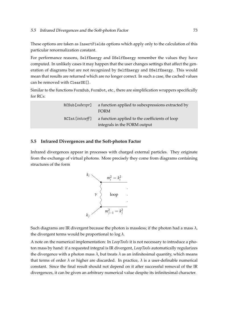
5.5 Infrared Divergences and the Soft-photon Factor 73
These options are taken as InsertFields options which apply only to the calculation of this
particular renormalization constant.
For performance reasons, SelfEnergy and DSelfEnergy remember the values they have
computed. In unlikely cases it may happen that the user changes settings that affect the gen-
eration of diagrams but are not recognized by SelfEnergy and DSelfEnergy. This would
mean that results are returned which are no longer correct. In such a case, the cached values
can be removed with ClearSE[].
Similar to the functions FormSub, FormDot, etc., there are simplification wrappers specifically
for RCs:
RCSub[subexpr] a function applied to subexpressions extracted by
FORM
RCInt[intcoeff] a function applied to the coefficients of loop
integrals in the FORM output
5.5 Infrared Divergences and the Soft-photon Factor
Infrared divergences appear in processes with charged external particles. They originate
from the exchange of virtual photons. More precisely they come from diagrams containing
structures of the form
.
.
.
ki
k j
γ loop
m2j−1 = k2
j
m2i = k2
i
Such diagrams are IR divergent because the photon is massless; if the photon had a mass λ,
the divergent terms would be proportional to log λ.
A note on the numerical implementation: In LoopTools it is not necessary to introduce a pho-
ton mass by hand: if a requested integral is IR divergent, LoopTools automatically regularizes
the divergence with a photon mass λ, but treats λ as an infinitesimal quantity, which means
that terms of order λ or higher are discarded. In practice, λ is a user-definable numerical
constant. Since the final result should not depend on it after successful removal of the IR
divergences, it can be given an arbitrary numerical value despite its infinitesimal character.
74 6 POST-PROCESSING OF THE RESULTS
The divergences in the diagrams with virtual photon exchange exactly cancel those in the
emission amplitude of soft (i.e. low-energetic) photons off the external legs. Soft-photon ra-
diation is always present experimentally: because photons are massless, they can have arbi-
trarily low energies and therefore escape undetected. So while the unphysical λ-dependence
cancels, the final result depends instead on a detector-dependent quantity Emaxsoft , the maxi-
mum energy a soft photon may have without being detected.
In a one-loop calculation one needs to take into account the bremsstrahlung off the Born
diagrams to be consistent in the order ofα. Dealing with soft photons is relatively easy since
the soft-photon cross-section is always proportional to the Born cross-section:
[dσ
dΩ
]
SB
= δSB
[dσ
dΩ
]
Born
where “SB” stands for soft bremsstrahlung.
The soft-photon factor δSB is implemented in main.F using the formulas of [De93]. It is
controlled by the following two preprocessor statements in process.h.
c#define BREMSSTRAHLUNG
#define ESOFTMAX .1D0*sqrtS
The first flag, BREMSSTRAHLUNG, is commented out by default. To switch on soft-photon cor-
rections, take out the c before the #define. The second line determines the energy cutoff
Emaxsoft .
6 Post-processing of the Results
6.1 Reading the data files into Mathematica
The format in which data are written out by main.F is directly practical only for making
plots of the cross-section over the energy or some phase-space variable. In many circum-
stances one needs to make more sophisticated figures in which the data are either arranged
differently, or are run through some filter or calculation. Consider, for example, performing
a scan over some region in parameter space and then wanting to plot the band of allowed
values of the cross-section, i.e. the minimum and maximum with respect to the parameter
variations for each point in phase space.
Given the variety of operations one could conceivably perform on the data, a Fortran or
C program would sooner or later prove too inflexible. Instead, there is a utility program
with which it is possible to read the data into Mathematica, where it is much easier to further
process the data sets and eventually produce plots of whatever function of whatever data
set one is interested in.

6.1 Reading the data files into Mathematica 75
The data files are read into Mathematica with the MathLink program ReadData, which is used
in the following way:
In[1]:= Install["ReadData"];
In[2]:= ReadData["run.UUUU.00300-01000.data"]
Out[2]= 24
The data are stored in Mathematica as separate data and parameter sets. These sets are ac-
cessed through an integer argument, e.g. Data[1] and Para[1]. ReadData returns the num-
ber of sets read (24 in this example).
The data files have to be roughly in the format used by main.F, i.e. a number of lines begin-
ning by # in which the parameters are given, followed by columns of data. The following
example shows this format:
# TB= 1.50
# MUE=-1000.00
# MSusy= 1000.00
# MA0= 700.00
# M_2= 100.00
160.790000000000 0.264226254743272 0.502096473139054
190.482475649966 10.7918866098049 9.58435238790029
211.567524166608 11.8170727823835 10.3862900941921
# TB= 1.50
# MUE=-1000.00
# MSusy= 1000.00
# MA0= 700.00
# M_2= 400.00
160.790000000000 0.264226254743272 0.502510502734037
190.482475649966 10.7918866098049 9.60119470492217
211.567524166608 11.8170727823835 10.4047052203442
The output of ReadData for this file is 2, hence there are then two data and two parameter
sets defined,
Para[1] = TB -> 1.5, MUE -> -1000., MSusy -> 1000.,
MA0 -> 700., M$2 -> 100.

76 6 POST-PROCESSING OF THE RESULTS
Data[1] = 160.79, 0.264226, 0.502096,
190.482, 10.7919, 9.58435,
211.568, 11.8171, 10.3863
Para[2] = TB -> 1.5, MUE -> -1000., MSusy -> 1000.,
MA0 -> 700., M$2 -> 400.
Data[2] = 160.79, 0.264226, 0.502511,
190.482, 10.7919, 9.60119,
211.568, 11.8171, 10.4047
Note that the numbers have not suffered in accuracy; it is a peculiarity of Mathematica to
display real numbers with no more than six digits by default. Note also that the underscore
in M_2 which is not allowed in symbol names in Mathematica has been replaced by a $.
ReadData[f, n, hpara, hdata] read the data file f into parameter and data sets in
Mathematica; with the optional parameters n, hpara,
and hdata one can choose to start numbering the sets
with n, use head hpara instead of Para, and use head
hdata instead of Data
Data[n] the nth data set
Para[n] the nth parameter set
In addition, ReadData has a handy way of applying operations to each line of data: it does
not, in fact, put each line of numbers in a list, but in a function called DataRow. By default,
DataRow is equal to List. Now consider that instead of the absolute values of the cross-
section, which is what main.F calculates by default, you want e.g. the relative deviation of
the one-loop and the tree-level cross-section. All it needs to achieve this is to redefine the
DataRow function as follows:
Clear[DataRow];
DataRow[x_, tree_, loop_] := x, loop/tree
(This works because main.F puts the tree-level result in the second column and the one-loop
correction in the third column.)
function default value
DataRow List the function which is applied to each
row of data in a file read by ReadData
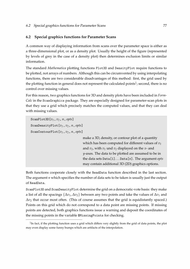
6.2 Special graphics functions for Parameter Scans 77
6.2 Special graphics functions for Parameter Scans
A common way of displaying information from scans over the parameter space is either as
a three-dimensional plot, or as a density plot. Usually the height of the figure (represented
by levels of grey in the case of a density plot) then determines exclusion limits or similar
information.
The standard Mathematica plotting functions Plot3D and DensityPlot require functions to
be plotted, not arrays of numbers. Although this can be circumvented by using interpolating
functions, there are two considerable disadvantages of this method: first, the grid used by
the plotting function in general does not represent the calculated points§; second, there is no
control over missing values.
For this reason, two graphics functions for 3D and density plots have been included in Form-
Calc in the ScanGraphics package. They are especially designed for parameter-scan plots in
that they use a grid which precisely matches the computed values, and that they can deal
with missing values.
ScanPlot3D[v1, v2, n, opts]
ScanDensityPlot[v1, v2, n, opts]
ScanContourPlot[v1, v2, n, opts]
make a 3D, density, or contour plot of a quantity
which has been computed for different values of v1
and v2, with v1 und v2 displayed on the x- and
y-axes. The data to be plotted are assumed to be in
the data sets Data[1]. . . Data[n]. The argument opts
may contain additional 3D (2D) graphics options.
Both functions cooperate closely with the ReadData function described in the last section.
The argument n which specifies the number of data sets to be taken is usually just the output
of ReadData.
ScanPlot3D and ScanDensityPlot determine the grid on a democratic-vote basis: they make
a list of all the spacings ∆v1,∆v2 between any two points and take the values of ∆v1 and
∆v2 that occur most often. (This of course assumes that the grid is equidistantly spaced.)
Points on this grid which do not correspond to a data point are missing points. If missing
points are detected, both graphics functions issue a warning and deposit the coordinates of
the missing points in the variable $MissingPoints for checking.
§In fact, if the plotting function uses a grid which differs very slightly from the grid of data points, the plot
may even display some funny bumps which are artifacts of the interpolation.
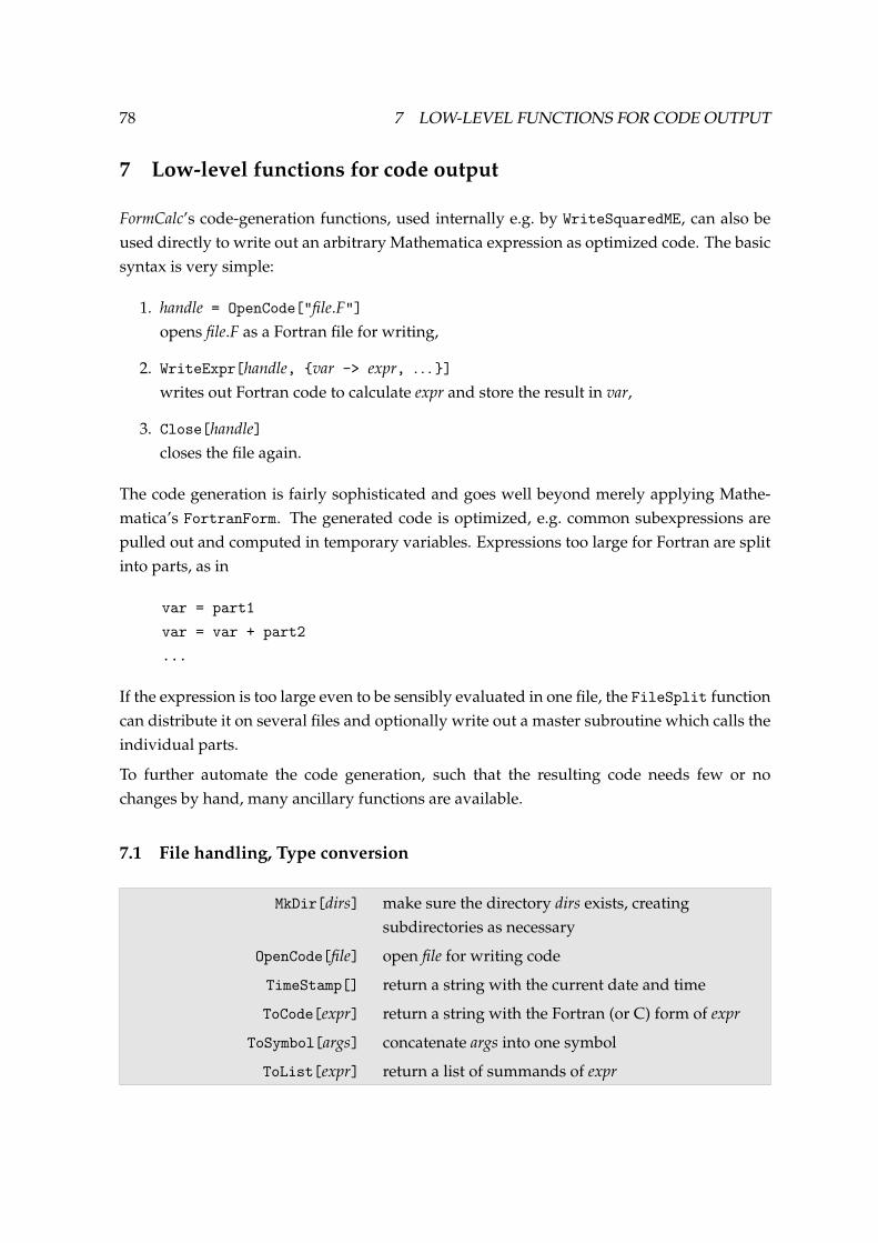
78 7 LOW-LEVEL FUNCTIONS FOR CODE OUTPUT
7 Low-level functions for code output
FormCalc’s code-generation functions, used internally e.g. by WriteSquaredME, can also be
used directly to write out an arbitrary Mathematica expression as optimized code. The basic
syntax is very simple:
1. handle = OpenCode["file.F"]
opens file.F as a Fortran file for writing,
2. WriteExpr[handle, var -> expr, . . . ]
writes out Fortran code to calculate expr and store the result in var,
3. Close[handle]
closes the file again.
The code generation is fairly sophisticated and goes well beyond merely applying Mathe-
matica’s FortranForm. The generated code is optimized, e.g. common subexpressions are
pulled out and computed in temporary variables. Expressions too large for Fortran are split
into parts, as in
var = part1
var = var + part2
...
If the expression is too large even to be sensibly evaluated in one file, the FileSplit function
can distribute it on several files and optionally write out a master subroutine which calls the
individual parts.
To further automate the code generation, such that the resulting code needs few or no
changes by hand, many ancillary functions are available.
7.1 File handling, Type conversion
MkDir[dirs] make sure the directory dirs exists, creating
subdirectories as necessary
OpenCode[file] open file for writing code
TimeStamp[] return a string with the current date and time
ToCode[expr] return a string with the Fortran (or C) form of expr
ToSymbol[args] concatenate args into one symbol
ToList[expr] return a list of summands of expr

7.2 Writing Expressions 79
MkDir["dir1", "dir2", . . . ] makes sure the directory dir1/dir2/. . . exists, creating the indi-
vidual subdirectories dir1, dir2, . . . as necessary. It works roughly as mkdir -p in Unix.
OpenCode[file] opens file for writing code.
TimeStamp[] returns a string with the current date and time.
ToCode[expr] returns the Fortran (or C) form of expr as a string.
ToSymbol[args] concatenates its arguments into a new symbol, e.g. ToSymbol[a, 1, x, y]
gives a1xy.
ToList[expr] returns a list of summands of expr, i.e. turns a sum of items into a list of items.
7.2 Writing Expressions
PrepareExpr[exprs] prepare exprs for write-out to code
WriteExpr[file, exprs] write exprs to file
CodeExpr[v, t, exprs] the expressions exprs with variables v and
temporary variables t in a form ready for write-out
by WriteExpr
RuleAdd[a,b] same as a -> a + b
DebugLine[s] a debugging statement for variable s
$SymbolPrefix a string prepended to all externally visible symbols
to avoid symbol conflicts
PrepareExpr[var1 -> expr1, var2 -> expr2, . . . ] prepares a list of variable assignments
for write-out to a code file. Expressions with a leaf count larger than $BlockSize are split
into several pieces, as in
var = part1
var = var + part2
...
thereby possibly introducing temporary variables for subexpressions. SumOver, DoLoop, and
IndexIf objects are properly taken into account as do-loops and if-statements. The output is
a CodeExpr[vars, tmpvars, exprlist] object, where vars are the original and tmpvars the tem-
porary variables introduced by PrepareExpr.
WriteExpr[file, exprlist] writes a list of variable assignments to file. The exprlist can either
be a CodeExpr object, i.e. the output of PrepareExpr, or a list of expressions of the form
var1 -> expr1, var2 -> expr2, . . . , which is first converted to a CodeExpr object using
PrepareExpr. WriteExpr returns a list of the subexpressions that were actually written.

80 7 LOW-LEVEL FUNCTIONS FOR CODE OUTPUT
CodeExpr[vars, tmpvars, exprlist] is the output of PrepareExpr and contains a list of expres-
sions ready to be written to a file, where vars are the original variables and tmpvars are tem-
porary variables introduced in order to shrink individual expressions to a size small enough
for Fortran.
RuleAdd[var, expr] is equivalent to var -> var + expr.
DebugLine[s] translates to a debugging statement for variable s (print-out of variable s) in
the code.
$SymbolPrefix is a string prepended to all externally visible symbols in the generated code
to avoid symbol collisions.
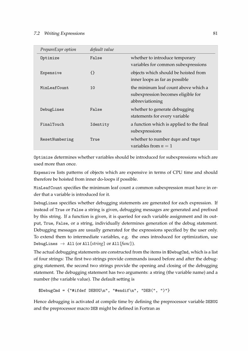
7.2 Writing Expressions 81
PrepareExpr option default value
Optimize False whether to introduce temporary
variables for common subexpressions
Expensive objects which should be hoisted from
inner loops as far as possible
MinLeafCount 10 the mininum leaf count above which a
subexpression becomes eligible for
abbreviationing
DebugLines False whether to generate debugging
statements for every variable
FinalTouch Identity a function which is applied to the final
subexpressions
ResetNumbering True whether to number dupn and tmpn
variables from n = 1
Optimize determines whether variables should be introduced for subexpressions which are
used more than once.
Expensive lists patterns of objects which are expensive in terms of CPU time and should
therefore be hoisted from inner do-loops if possible.
MinLeafCount specifies the minimum leaf count a common subexpression must have in or-
der that a variable is introduced for it.
DebugLines specifies whether debugging statements are generated for each expression. If
instead of True or False a string is given, debugging messages are generated and prefixed
by this string. If a function is given, it is queried for each variable assignment and its out-
put, True, False, or a string, individually determines generation of the debug statement.
Debugging messages are usually generated for the expressions specified by the user only.
To extend them to intermediate variables, e.g. the ones introduced for optimization, use
DebugLines → All (or All[string] or All[func]).
The actual debugging statements are constructed from the items in $DebugCmd, which is a list
of four strings: The first two strings provide commands issued before and after the debug-
ging statement, the second two strings provide the opening and closing of the debugging
statement. The debugging statement has two arguments: a string (the variable name) and a
number (the variable value). The default setting is
$DebugCmd = "#ifdef DEBUG\n", "#endif\n", "DEB(", ")"
Hence debugging is activated at compile time by defining the preprocessor variable DEBUG
and the preprocessor macro DEB might be defined in Fortran as

82 7 LOW-LEVEL FUNCTIONS FOR CODE OUTPUT
#define DEB(a,x) print *, a, x
FinalTouch gives a function which is applied to each final subexpression, just before write-
out to file.
ResetNumbering resets the internal numbering of variable names created by PrepareExpr,
i.e. variables of the form dupn (from Optimize) and tmpn (from Expensive) start at n = 1. It
may be necessary to disable this reset e.g. if more than one generated expression shall be put
in the same program unit.
Note: these options may also be given to WriteExpr which simply hands them down to
PrepareExpr. They cannot be set using SetOptions[WriteExpr, ...], however.
WriteExpr option default value
HornerStyle True whether to order expressions according
in Horner form
FinalCollect False whether to collect factors in the final
expression
FinalFunction Identity a function to apply to the final
expression before write-out
Type False the type of the expressions, False to
omit declarations
TmpType "ComplexType" the type of temporary variables
IndexType False the type of indices
RealArgs A0,A00,B0,B1, functions whose arguments must be
B00,B11,B001, of a guaranteed type (default: real)
B111,DB0,DB1,
DB00,DB11,
B0i,C0i,D0i,
E0i,F0i,Bget,
Cget,Dget,Eget,
Log,Sqrt
Newline "" a string to be printed after each
expression
HornerStyle specifies whether expressions are ordered in Horner form before writing them
out as code.
FinalCollect chooses a final collecting of common factors, after going over to Horner form,
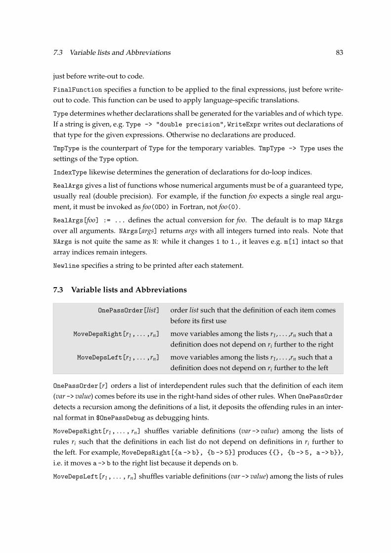
7.3 Variable lists and Abbreviations 83
just before write-out to code.
FinalFunction specifies a function to be applied to the final expressions, just before write-
out to code. This function can be used to apply language-specific translations.
Type determines whether declarations shall be generated for the variables and of which type.
If a string is given, e.g. Type -> "double precision", WriteExpr writes out declarations of
that type for the given expressions. Otherwise no declarations are produced.
TmpType is the counterpart of Type for the temporary variables. TmpType -> Type uses the
settings of the Type option.
IndexType likewise determines the generation of declarations for do-loop indices.
RealArgs gives a list of functions whose numerical arguments must be of a guaranteed type,
usually real (double precision). For example, if the function foo expects a single real argu-
ment, it must be invoked as foo(0D0) in Fortran, not foo(0).
RealArgs[foo] := ... defines the actual conversion for foo. The default is to map NArgs
over all arguments. NArgs[args] returns args with all integers turned into reals. Note that
NArgs is not quite the same as N: while it changes 1 to 1., it leaves e.g. m[1] intact so that
array indices remain integers.
Newline specifies a string to be printed after each statement.
7.3 Variable lists and Abbreviations
OnePassOrder[list] order list such that the definition of each item comes
before its first use
MoveDepsRight[r1, . . . ,rn] move variables among the lists r1, . . . ,rn such that a
definition does not depend on ri further to the right
MoveDepsLeft[r1, . . . ,rn] move variables among the lists r1, . . . ,rn such that a
definition does not depend on ri further to the left
OnePassOrder[r] orders a list of interdependent rules such that the definition of each item
(var -> value) comes before its use in the right-hand sides of other rules. When OnePassOrder
detects a recursion among the definitions of a list, it deposits the offending rules in an inter-
nal format in $OnePassDebug as debugging hints.
MoveDepsRight[r1, . . . , rn] shuffles variable definitions (var -> value) among the lists of
rules ri such that the definitions in each list do not depend on definitions in ri further to
the left. For example, MoveDepsRight[a -> b, b -> 5] produces , b -> 5, a -> b,
i.e. it moves a -> b to the right list because it depends on b.
MoveDepsLeft[r1, . . . , rn] shuffles variable definitions (var -> value) among the lists of rules

84 7 LOW-LEVEL FUNCTIONS FOR CODE OUTPUT
ri such that the definitions in each list do not depend on definitions in ri further to the
right. For example, MoveDepsLeft[a -> b, b -> 5] produces b -> 5, a -> b, , i.e.
it moves b -> 5 to the left list because that depends on b.
SplitSums[expr] split expr into a list of expressions such that index
summations apply to the whole of each part
ToDoLoops[list] categorize list into patches that must be summed
over the same set of indices
DoLoop[expr, ind] a do-loop of expr over the indices ind
SplitSums[expr] splits expr into a list of expressions such that index sums (marked by
SumOver) always apply to the whole of each part. SplitSums[expr,wrap] applies wrap to
the coefficients of the SumOver.
ToDoLoops[list, ifunc] splits list into patches which must be summed over the same set of
indices. ifunc is an optional argument: ifunc[expr] must return the indices occurring in expr.
DoLoop[ind, expr] is a symbol introduced by ToDoLoops indicating that expr is to be summed
over the set of indices ind.
ToIndexIf[expr] turn the IndexDelta and IndexDiff in expr into
IndexIf
IndexIf[cond, a, b] same as If[cond, a, b] except that the expressions a
and b are not held unevaluated
IndexDelta[i, j] Kronecker’s δij
IndexDiff[i, j] 1 − δij
MapIf[f, expr] maps f over the expr except for the conditional parts
of an IndexIf
ToIndexIf[expr] converts all IndexDelta and IndexDiff objects in expr to IndexIf, which
will be written out as if-statements in the generated code. ToIndexIf[expr, patt] operates
only on indices matching patt.
IndexIf[cond, a, b] is the same as If[cond, a, b] except that expressions a and b are not
held unevaluated. IndexIf[cond, a] is equivalent to IndexIf[cond, a, 0], i.e. the “else” part
defaults to 0. Several conditions can be combined as IndexIf[cond1, a1, cond2, a2, . . . ],
which is equivalent to IndexIf[cond1, a1, IndexIf[cond2, a2, . . . ]]. Despite its name, the
statement is not restricted to index nor to integer comparisons. It is furthermore written out
as a regular if statement, i.e.
if( cond ) then
a
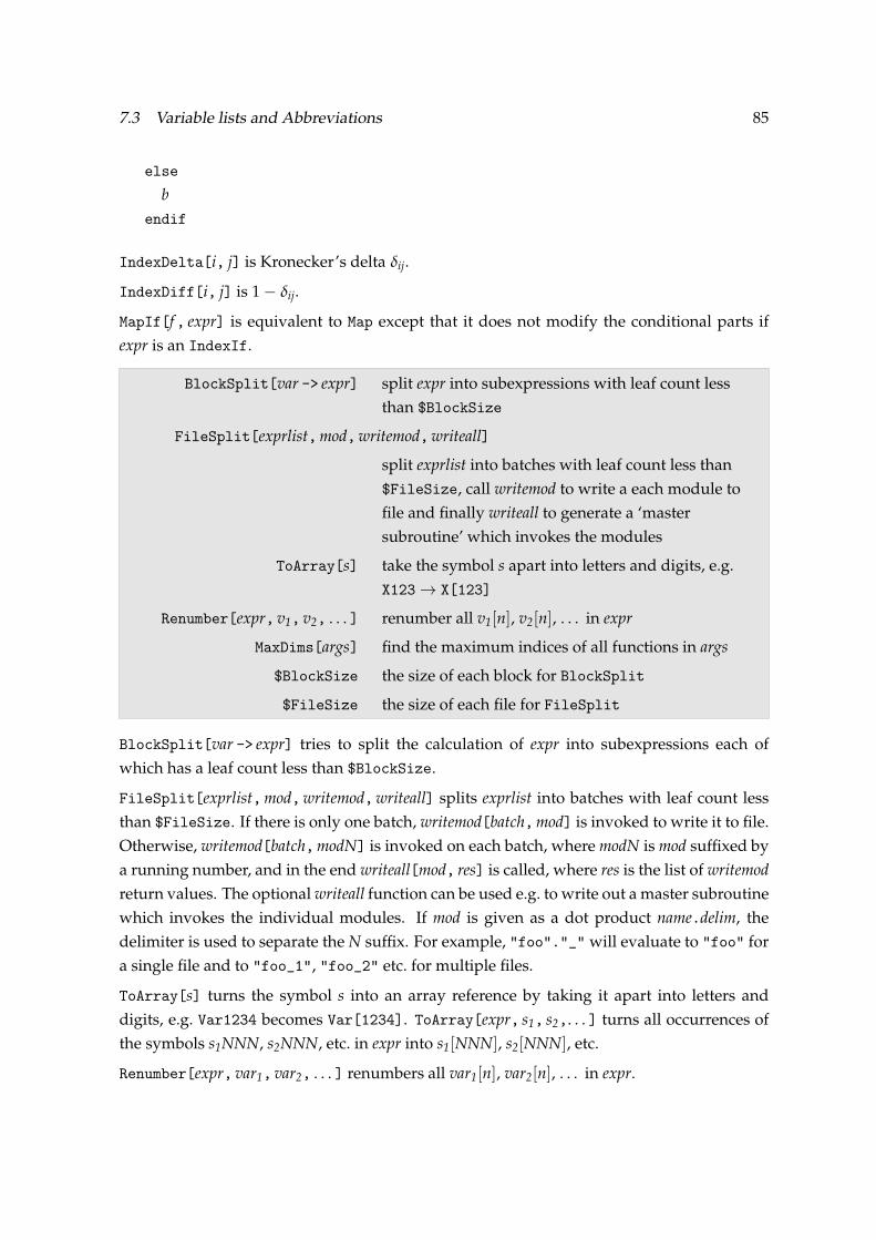
7.3 Variable lists and Abbreviations 85
else
b
endif
IndexDelta[i, j] is Kronecker’s delta δij.
IndexDiff[i, j] is 1 − δij.
MapIf[f, expr] is equivalent to Map except that it does not modify the conditional parts if
expr is an IndexIf.
BlockSplit[var -> expr] split expr into subexpressions with leaf count less
than $BlockSize
FileSplit[exprlist,mod,writemod,writeall]
split exprlist into batches with leaf count less than
$FileSize, call writemod to write a each module to
file and finally writeall to generate a ‘master
subroutine’ which invokes the modules
ToArray[s] take the symbol s apart into letters and digits, e.g.
X123 → X[123]
Renumber[expr, v1, v2, . . . ] renumber all v1[n], v2[n], . . . in expr
MaxDims[args] find the maximum indices of all functions in args
$BlockSize the size of each block for BlockSplit
$FileSize the size of each file for FileSplit
BlockSplit[var -> expr] tries to split the calculation of expr into subexpressions each of
which has a leaf count less than $BlockSize.
FileSplit[exprlist,mod,writemod,writeall] splits exprlist into batches with leaf count less
than $FileSize. If there is only one batch, writemod[batch,mod] is invoked to write it to file.
Otherwise, writemod[batch,modN] is invoked on each batch, where modN is mod suffixed by
a running number, and in the end writeall[mod, res] is called, where res is the list of writemod
return values. The optional writeall function can be used e.g. to write out a master subroutine
which invokes the individual modules. If mod is given as a dot product name.delim, the
delimiter is used to separate the N suffix. For example, "foo"."_" will evaluate to "foo" for
a single file and to "foo_1", "foo_2" etc. for multiple files.
ToArray[s] turns the symbol s into an array reference by taking it apart into letters and
digits, e.g. Var1234 becomes Var[1234]. ToArray[expr, s1, s2,. . . ] turns all occurrences of
the symbols s1NNN, s2NNN, etc. in expr into s1[NNN], s2[NNN], etc.
Renumber[expr, var1, var2, . . . ] renumbers all var1[n], var2[n], . . . in expr.

86 7 LOW-LEVEL FUNCTIONS FOR CODE OUTPUT
MaxDims[args] returns a list of all distinct functions in args with the highest indices that
appear, e.g. MaxDims[foo[1, 2], foo[2, 1]] returns foo[2, 2].
7.4 Declarations
SubroutineDecl[name] the declaration for the subroutine name
VarDecl[vars, type︸ ︷︷ ︸a
] the declaration of vars as variables of type type
VarDecl[Common[com][a]] the declaration of common block com with
individual variables a (a as above)
VarDecl[NameMap[com][a]] the declaration of common block com with an array
plus a preprocessor map of the a onto array
elements (a as above)
VarDecl[NotEmpty[a]] output only if at least one variable list in a is
non-empty
DoDecl[i, range] the declaration of a do-loop of i over range
CallDecl[subs] the invocations of subroutines subs
Dim[i] the highest value the index i takes on
SubroutineDecl[name] returns a string with the declaration of the subroutine name.
VarDecl[v1 , v2, . . ., t] returns a string with the declaration of v1, v2, . . . as variables of type
t. Any other strings are output verbatim, e.g. "#ifdef COND\n", "#endif\n".
VarDecl[Common[c][v1 , v2, . . ., t]] declares v1, v2, . . . to be members of common block c.
VarDecl[NameMap[c][v1 , v2, . . ., t]] works much like Common but puts only arrays into the
common block (one for each data type), together with preprocessor statements mapping the
v1, v2, . . . onto array elements.
VarDecl arguments wrapped in NotEmpty are output only if at least one of its variable lists
is non-empty.
DoDecl[i,m] returns a string with the declaration of a loop over i from 1 to m.
DoDecl[i, a, b] returns the same for a loop from a to b. DoDecl[i] invokes Dim[i] to de-
termine the upper bound on i.
CallDecl[sub1, sub2, ...] returns a string with the invocations of the subroutines sub1,
sub2, . . . , taking into account possible loops indicated by DoLoop.
Dim[i] returns the highest value the index i takes on, as determined from the amplitude
currently being processed.

7.5 Compatibility Functions 87
7.5 Compatibility Functions
ToOldBRules rules to convert to the conventions for two-point
functions of LoopTools 2.2 and before
ToNewBRules rules to convert to the conventions for two-point
functions of LoopTools 2.3 or later
ToOldBRules and ToNewBRules are two sets of transformation rules that convert between the
old (B0, B1, . . . ) and new (B0i[b0,b1,. . . ]) conventions for two-point functions in LoopTools.

88 REFERENCES
References
[Ch79] M. Chanowitz, M. Furman, and I. Hinchliffe, Nucl. Phys. B159 (1979) 225.
[Cv76] P. Cvitanovic, Phys. Rev. D14 (1976) 1536.
[dA98] F. del Aguila, A. Culatti, R. Munoz Tapia, and M. Perez-Victoria, Nucl. Phys. B537
(1999) 561 [hep-ph/9806451].
[De93] A. Denner, Fortschr. Phys. 41 (1993) 307.
[Ha98] T. Hahn and M. Perez-Victoria, Comp. Phys. Commun. 118 (1999) 153
[hep-ph/9807565].
[Ha00] T. Hahn, Comp. Phys. Commun. 140 (2001) 418 [hep-ph/0012260].
[Ha02] T. Hahn, Nucl. Phys. Proc. Suppl. 116 (2003) 363 [hep-ph/0210220].
[Ha04] T. Hahn, Comp. Phys. Commun. 168 (2005) 78 [hep-ph/0404043].
[Ha04a] T. Hahn, Nucl. Phys. Proc. Suppl. 135 (2004) 333 [hep-ph/0406288].
[Ha06] T. Hahn, physics/0607103.
[Ni05] C.C. Nishi, Am. J. Phys. 73 (2005) 1160 [hep-ph/0412245].
[Si79] W. Siegel, Phys. Lett. B84 (1979) 193.
[tH72] G. ’t Hooft and M. Veltman, Nucl. Phys. B44 (1972) 189.
[Ve00] J.A.M. Vermaseren, math-ph/0010025. See also http://www.nikhef.nl/~form.
[Ve96] J.A.M. Vermaseren, The use of computer algebra in QCD, in: H. Latal, W. Schweiger,
Proceedings Schladming 1996, Springer Verlag, ISBN 3-540-62478-3.
[WhBG05] M.R. Whalley, D. Bourilkov, R.C. Group, hep-ph/0508110.
http://hepforge.cedar.ac.uk/lhapdf/.
[Za03] A.F. Zarnecki, Acta Phys. Polon. B34 (2003) 2741 [hep-ex/0207021].
Acknowledgements
FormCalc would not be able to calculate in four dimensions without the hard work of Manuel
Perez-Victoria and his deep understanding of constrained differential renormalization.
The fermionic matrix elements would not be half as well implemented without the relentless
testing of Christian Schappacher.

Index
’t Hooft–Veltman scheme, 13
$AbbPrefix, 25
$DriversDir, 41
$Editor, 13
$EditorModal, 13
$FormAbbrDepth, 14
$FormCmd, 7
$OptPrefix, 24
1to2.F,.h, 40
2to2.F,.h, 40
2to3.F,.h, 40
Abbr, 24
AbbrevDo, 25
Abbreviate, 25
abbreviations, 6, 23, 30
registering, 27
AbbrevSet, 25
Alfa, 21
Alfa2, 21
Alfas, 21
Alfas2, 21
All, 30, 32
analytic amplitudes, 36
antisymmetrization, 16
Antisymmetrize, 15
ApplyUnitarity, 38
Automatic, 10
bfunc.m, 40
Breitenlohner–Maison scheme, 13
btensor.m, 40
C code, 41
CA2, 22
CalcFeynAmp, 8, 14
CalcLevel, 10
cancellation of terms, 11
CB2, 22
CBA2, 22
Chiral, 11
chirality projector, 20
Classes, 10
ClearProcess, 16
code generation, 41
colour indices, 19, 32
ColourGrouping, 32
ColourME, 32
ColourSimplify, 32
Combine, 16
compiling, 7
components, 36
configure, 40
constrained differential
renormalization, 6, 10
CutTools, 12
Cvitanovic algorithm, 32
CW2, 21
data, 40
debugging options, 13
DeclareProcess, 14
demo programs, 6
Den, 18
DenCollect, 38
denominator, 18
density matrix, 29
Deny, 26
diagram generation, 7
DiagramType, 17
Dimension, 10, 31, 35
dimension, 22
dimensional
reduction, 6, 10
regularization, 6, 10
89

90 INDEX
Dirac equation, 8
Dirac matrix, 20
DiracChain, 20
Divergence, 37
Dminus4, 11, 31, 35, 37
Dminus4Eps, 31, 35
dot product, 18
DotExpand, 10, 31, 35
DottedSpinor, 21
Drivers, 41
drivers, 40
e[n], 18
EditCode, 10, 31, 35
Eps, 18
Evanescent, 10
ExceptDirac, 15
ExpandSums, 38
expansion, 13
external fermions, 28
external spinors, 11
fermion chain, 11
fermion traces, 8
FermionChains, 10
fermionic matrix elements, 28
FermionicQ, 17
FermionOrder, 10
FeynArts, 7
Fierz transformation, 11
FileTag, 10
Finite, 18
FormAmp, 15
FormDot, 14
FormMat, 14
FormPre, 14
FormQC, 14
FormQF, 14
FormSub, 14
Fortran code, 41
four-vector, 36
Fuse, 26
Gamma5Test, 10
Gamma5ToEps, 10
GaugeTerms, 35
generators of SU(N), 19
generic amplitude, 7
gluon indices, 32
Gram determinant, 18
Hel[n], 30
helicity, 29
helicity matrix elements, 29
helicity reference vector, 29
HelicityME, 11, 14, 30
IGram, 18
index contractions, 8
InsertionPolicy, 10
insertions, 12
installation, 7
internal definitions, 16
Invariants, 15
invariants, 15
simplification, 16
inverse Gram, 18
InvSimplify, 15
k[n], 18
Keep, 28
kinematical simplification, 12
kinematics, 16, 18
leaf count, 24
levels in diagrams, 7, 10
Levi-Civita tensor, 18
local terms, 8
loop integral
symmetrized, 12
Lor[n], 20
INDEX 91
Lorentz index, 20
lumi_hadron.F, 40
lumi_parton.F, 40
lumi_photon.F, 40
MA02, 22
main.F,.h, 40
makefile.in, 40
Mandelstam variables, 15, 19, 23
mass shell, 15
MassDim, 22
MassDim0, 22
MassDim1, 22
MassDim2, 22
Mat, 30, 32, 33
MB2, 21
MC2, 21
MCha2, 22
MD2, 21
ME2, 21
MG02, 22
MGl2, 22
MGp2, 22
Mh02, 22
MH2, 21
MHH2, 22
MHp2, 22
MinLeafCount, 26
mktm, 40
ML2, 21
MLE2, 21
MM2, 21
MNeu2, 22
model parameters, 21
model-dependent symbols, 23
model_mssm.F, 40
model_sm.F, 40
model_thdm.F, 40
MomElim, 10, 31, 35
momenta, 18
momentum conservation, 11
MomRules, 10
MQD2, 21
MQU2, 21
MS2, 21
MSf2, 22
MSSMSimplify, 22
MT2, 21
MU2, 21
MultiplyDiagrams, 17
MW2, 21
MZ2, 21
Neglect, 22
neglecting masses, 22
NoBracket, 10, 35
NoCostly, 10
NoExpand, 10
non-expansion of terms, 13
normalization, 15
Normalized, 15
numbering of momenta, 18
numerator function, 12
numerical evaluation, 6, 39
OffShell, 17
on-shell particles, 15
OnShell, 15
OnSize, 38
open fermion chains, 8
OPP, 12
OPP, 10
OPPQSlash, 10
OptimizeAbbr, 24
ordering, 11
Pair, 18
Particles, 10
PaVeReduce, 10
92 INDEX
pnuglot, 40
polarization sum, 34
polarization vector, 15, 18
PolarizationSum, 14, 34
Pool, 38
PostFunction, 10
PreFunction, 10
Preprocess, 26
process.h, 40
propagator denominator, 18
rational terms, 12
ReadData.tm, 40
ReadFormDebug, 13
RegisterAbbr, 27
registering abbreviations, 27
RegisterSubexpr, 27
regularization method, 10
reorder.c, 40
RetainFile, 10, 31, 35
run.F, 40
S, 19
s[n], 18, 30
SA2, 22
Samurai, 12
SB2, 22
SBA2, 22
ScanGraphics.m, 40
selecting diagrams, 17
SetupCodeDir, 41
sfx, 40
short-hands, 23
Sij, 19
SimplifyQ2, 10
size of the amplitude, 24
SMSimplify, 21
SortDen, 10
spin, 29
Spinor, 20, 21
spinor chain, 11, 28
squared matrix element, 33
SquaredME, 33
SU(N) objects, 19, 32
SubExpr, 27
subexpressions
registering, 27
submit, 40
SumLegs, 35
SUNN, 19
SUNT, 19, 32
SUSYTrigExpand, 22
SUSYTrigReduce, 22
SUSYTrigSimplify, 22
SW2, 21
T, 19
TagCollect, 38
TagDiagrams, 17
TB2, 22
tensor coefficients, 12
tensor reduction, 8
test, γ5, 12
Tij, 19
ToComponents, 36
tools, 40
transversality, 15
Transverse, 15
turnoff, 40
U, 19
UChaC, 22
ultraviolet divergences, 37
unpolarized case, 29
unsquared, 36
useful functions, 38
USfC, 22
UV divergences, 10
UVDivergentPart, 37
UVSeries, 37
INDEX 93
VA, 11
VChaC, 22
VecSet, 36
vector, 36
Weyl, 11
WeylChain, 21
WriteRenConst, 41
WriteSquaredME, 41
xsection.F,.h, 40
ZNeuC, 22