formulation of optimal semi-active feedback by...

GSC’17 - Graduate Students in Control

Formulation of Optimal Semi-Active Feedback byKrotov’s Method

I. Halperin, G. Agranovich, Y. Ribakov

May 8 2017,Haifa, Israel

1 Introduction

2 Aims and Scope

3 Optimal Control Problem - CBQR

4 Optimal Control Theory

5 Main Results

6 Numerical Example

7 Conclusions

2 / 38

Introduction

Vibration control.Structural control - a branch of vibration control. Exploits controltheory to enhance dynamic response of structures. Mostly thoseinduced by winds, earthquakes and man.

Ji-Ji earthquakeTaiwan, 1999

Man induced vibration

Common structural control realization consists of mechanicalactuators which apply forces to the vibrating structure.

3 / 38

fig/Eintracht Frankfurt fans moving stands while jumping-5z5mbCWThZ8.mp4

Introduction

A simplified block diagram of a controlled structure:

Plant

Actuator

Controller Sensors

x(t)g(t), x(0)

w(t)

g

x(0)

4 / 38

Introduction

Semi-active dampers are type of actuators which are characterized bylow energy consumption, dissipativity and inherent stability.

Variable Orifice MR

PneumaticVariable Viscous

5 / 38

Introduction

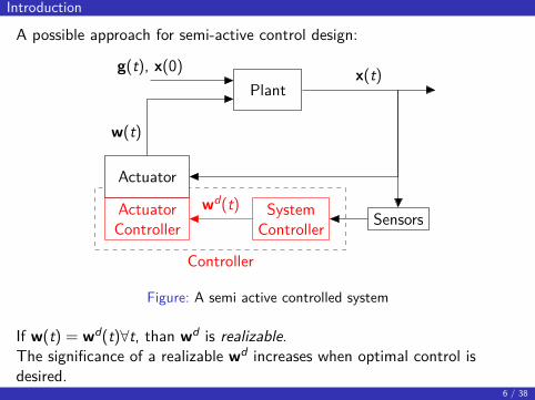
A possible approach for semi-active control design:

Controller

Plant

Actuator

ActuatorController

SystemController Sensors

x(t)g(t), x(0)

w(t)

wd(t)

Figure: A semi active controlled system

If w(t) = wd(t)∀t, than wd is realizable.The significance of a realizable wd increases when optimal control isdesired.

6 / 38

Introduction

In order to compute a realizable wd, the system controller must considerthe actuator constraints.For semi-active controlled plants, it must consider a fundamentalsemi-active constraint.

z(t)

w(t): compressive force

Definition 1 (Semi-Active Constraint).

w(t)z(t) ≤ 0orw(t)cx(t) ≤ 0

7 / 38

1 Introduction

2 Aims and Scope



5 Main Results

6 Numerical Example

7 Conclusions

8 / 38

Aims and Scope

To compute a realizable optimal feedback for mechanical plant, which iscontrolled by a single semi-active damper.The solution consists of two key stages:

1 Reformulation of the problem by writing the linear state equation asan equivalent bilinear one.

2 Using Krotov’s method to derive an algorithm for the computation ofan optimal semi-active feedback.

9 / 38

1 Introduction

2 Aims and Scope



5 Main Results

6 Numerical Example

7 Conclusions

10 / 38

Optimal Control Problem - Plant Model

The DOF model for free vibrating linear structure, equipped with a singleactuator:

Mz(t) + Cdz(t) + Kz(t) = ϕw(t); z(0), z(0) ∈ Rnz , ∀t ∈ (0, tf) (1)

where M > 0, Cd ≥ 0 and K > 0 are nz × nz; nz is the number of dynamicdegrees of freedom (DOF); z : [0, tf ] → Rnz is a smooth vector function ofthe DOF displacements; w : [0, tf ] → R is a control force signal andϕ ∈ Rnz is an input vector that describes how the control force affects thestructure’s DOF. The state space model:

x(t) =Ax(t) + bw(t); x(0); x(t) =[z(t)z(t)

](2a)

A ≜[

0 I−M−1K −M−1Cd

]∈ Rn×n (2b)

b ≜[

0M−1ϕ

]∈ Rn (2c)

11 / 38

Optimal Control Problem - CBQR

By writing w in the bilinear form:

w(t) = w(t, x(t)) = −u(t)cx(t); u(t) ≥ 0

we are assured that the semi-active constraint is intrinsically satisfied.

Definition 2 (CBQR).A constrained bilinear quadratic regulator refers to the minimization of

J(x, u) =12

tf∫0

x(t)TQx(t) + ru(t)2d t; Q ≥ 0, r > 0

subjected to

x(t) = [A − u(t)bc]x(t), x(0); u(t) ≥ 0

12 / 38

1 Introduction

2 Aims and Scope



5 Main Results

6 Numerical Example

7 Conclusions

13 / 38

Optimal Control Theory

V. F. Krotov(1932-2015)

Starting in the sixties, sufficient conditions for global optimum ofoptimal control problems were published by V. F. Krotov 1 .It enabled the computation of a global optimum by an algorithmwhich is known as global method of successive improvements ofcontrol or Krotov’s method.

1V. F. Krotov, Global Methods in Optimal Control Theory, 1995.14 / 38

Optimal Control Theory

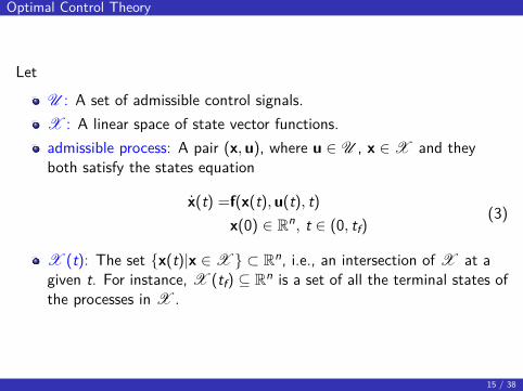
LetU : A set of admissible control signals.X : A linear space of state vector functions.admissible process: A pair (x,u), where u ∈ U , x ∈ X and theyboth satisfy the states equation

x(t) =f(x(t),u(t), t)x(0) ∈ Rn, t ∈ (0, tf)

(3)

X (t): The set {x(t)|x ∈ X } ⊂ Rn, i.e., an intersection of X at agiven t. For instance, X (tf) ⊆ Rn is a set of all the terminal states ofthe processes in X .

15 / 38

Optimal Control Theory - Krotov’s Sufficient Condition

q: A piecewise smooth function Rn × R → R, denoted as Krotovfunction or solving function. Its partial derivatives are denoted by qtand qx.J: A performance index. It is a functional

J(x,u) =lf (x(tf)) +

tf∫0

l(x(t),u(t), t)d t

where lf : Rn → R and l : Rn × Rnu × R → R are continuous.Each q is related with an equivalent formulation of performance index, asfollows.

16 / 38


Theorem 3.Let (x,u) be an admissible process. For each q there is an equivalentrepresentation of J(x,u):

Jeq(x,u) =sf (x(tf)) + q(x(0), 0) +tf∫

0

s(x(t),u(t), t)d t ≡ J(x,u) (4)

s(x(t),u(t), t) ≜qt(x(t), t) + qx(x(t), t)f(x(t),u(t), t)+ l(x(t),u(t), t)

(5a)

sf (x(tf)) ≜lf (x(tf))− q(x(tf), tf) (5b)

Proof.Substitute s and sf in Jeq, and then use Newton-Leibniz formula.

17 / 38


It should be stressed that J(x,u) = Jeq(x,u) holds if x and u satisfythe state equation (Eq. (3)).As q is not unique, the equivalent representation Jeq, s and sf, arealso non-unique.In many publications, s is written with an opposite sign before l,Though, there is no intrinsic difference between these twoformulations.

18 / 38


Sufficient condition for a global optimal admissible process, by means ofJeq, is given by:

Theorem 4.Let s and sf be related with some q. Let (x∗,u∗) be an admissible process.If:

s(x∗(t),u∗(t), t) = minx(t)∈X (t)u(t)∈U (t)

s(x(t),u(t), t) ∀t ∈ [0, tf)

sf (x∗(tf)) = minx(tf)∈X (tf)

sf (x(tf))(6)

then (x∗,u∗) is an optimal process.

Proof.Assume that Eq. (6) holds and expand the differenceJeq(x,u)− Jeq(x∗,u∗).

19 / 38


An optimum derived by theorem 4 is global since the minimizationproblem defined in Eq. (6) is global.Theorems 4 and 3 provide a hint for finding a global optimum. Thatis, one should formulate q such that it will be possible to compute(x∗,u∗) from:

s(x∗(t),u∗(t), t) = minx(t)∈X (t)u(t)∈U (t)

s(x(t),u(t), t) ∀t ∈ [0, tf)

sf (x∗(tf)) = minx(tf)∈X (tf)

sf (x(tf))

However, the main problem remains - the existence and formulationof such q. Note that a similar approach is used in Lyapunov’s methodof stability.

20 / 38

Optimal Control Theory - Krotov’s Method

Krotov’s sufficient condition lays the foundation for novel algorithmsfor the solution of optimal control problems. Krotov’s method is oneof them.According to this method, the solution is not direct but a sequentialone. It yields a sequence of admissible processes which convergesmonotonically to an optimum (x∗,u∗). Such a sequence of processesis called an optimizing sequence:

(xk,uk) → (x∗,u∗); J(xk,uk) ≥ J(xk+1,uk+1)

s.t.x∗(t) = f(x∗(t),u∗(t), t); u∗ = argmin

x,uJ(x,u)

The use of Krotov’s method relies on the solution of another keyproblem which is the formulation of a sequence of solving functions -{qk}.

21 / 38


u: A control signal, i.e. a mapping R → Rnu .u: A control law, i.e. a mapping Rn × R → Rnu .

Let (x0,u0) be some initial admissible process. An improved process(x1,u1) is computed in the following manner:

1 Formulate q0 such that s0 and sf 0 will satisfy:

s0(x0(t),u0(t), t) = maxx∈X (t)

s0(x,u0(t), t) ∀t ∈ [0, tf)

sf 0(x0(tf)) = maxx∈X (tf)

sf 0(x)

2 Formulate a control law u0 such that

u0(x(t), t) = arg minu∈U (t)

s0(x(t),u, t) ∀x ∈ X , t ∈ [0, tf ]

3 Solve x1(t) = f(x1(t), u0(x1(t), t), t), for the given x(0), and setu1(t) = u0(x1(t), t) for all t ∈ [0, tf ].

(x2,u2) is computed by starting over from (x1,u1), formulation of q1 andu1, and so on.

22 / 38


The use of Krotov’s method is not straightforward. It requires theformulation of a suitable sequence {qk}, such that sk and sfk willsatisfy the aforementioned min/max problem.The search for such a sequence is a significant challenge. There is noknown unified approach for formulating Krotov functions and theyusually differ from one optimal control problem to another.In this work, a suitable sequence of Krotov functions was found forthe defined CBQR problem.

23 / 38

1 Introduction

2 Aims and Scope



5 Main Results

6 Numerical Example

7 Conclusions

24 / 38

Main Results

The next theorem defines the CBQR control law (step 2 in Krotov’smethod).

Theorem 5.

Let the Krotov function be

q(x(t), t) = 0.5x(t)TP(t)x(t); P(tf) = 0 (7)

where P : R → Rn×n is a symmetric matrix function, smooth above (0, tf);and let x be a given process. There exists a unique control law thatminimizes s(x(t), u(t), t) and sf(x(tf)). It is defined by:

u(x(t), t) = max

{x(t)TP(t)bcx(t)

r , 0}

(8)

Proof.By substitution of Eq. (7) in Eq. (5a) and (5b); completing the squareand minimizing with relation to an admissible u(t).

25 / 38

Main Results

The next theorem defines qk that corresponds (xk,uk) (step 1 in Krotov’smethod).

Theorem 6.

Let (xk, uk) be a given admissible process and let Pk be the solution of:

Pk(t) =− Pk(t)[A − uk(t)bc]− [AT − uk(t)cTbT]Pk(t)− QPk(tf) =0; t ∈ (0, tf)

(9)

The Krotov function qk(x(t), t) = 0.5x(t)TPk(t)x(t) satisfies

sk(xk(t), uk(t), t) = maxx∈X (t)

sk(x, uk(t), t) (10)

Proof.By substitution of qk,f,l in Eq. (5a) and using Eq. (9).

26 / 38

Main Results

The dependency of Krotov’s method on a Krotov function makes itsomewhat abstract. Theorems 5 and 6 turn it into a concrete solutionmethod for the addressed CBQR problem.As J has a lower bound, we are assured that the sequence {(xk, uk)}gets arbitrary close to some admissible process (x∗, u∗), which is theoptimal one.

27 / 38

Main Results - Successive improvement of control process.

Input: A,b, c,Q, r, x(0).Initialization:

1 Define a convergence tolerance - ϵ > 0.2 Set u0 = 0 and solve:

x0(t) =Ax0(t); x(0)P0(t) =− P0(t)A − ATP0(t)− Q; P0(tf) = 0

3 Compute:

J0(x0, u0) =12

tf∫0

x0(t)TQx0(t)d t

28 / 38


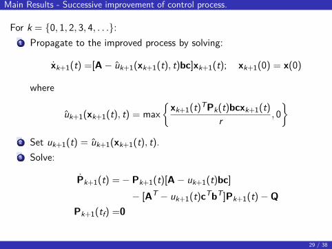
For k = {0, 1, 2, 3, 4, . . .}:1 Propagate to the improved process by solving:

xk+1(t) =[A − uk+1(xk+1(t), t)bc]xk+1(t); xk+1(0) = x(0)

where

uk+1(xk+1(t), t) = max

{xk+1(t)TPk(t)bcxk+1(t)

r , 0}

2 Set uk+1(t) = uk+1(xk+1(t), t).3 Solve:

Pk+1(t) =− Pk+1(t)[A − uk+1(t)bc]− [AT − uk+1(t)cTbT]Pk+1(t)− Q

Pk+1(tf) =0

29 / 38


4 Compute:

J(xk+1, uk+1) =12

tf∫0

xk+1(t)TQxk+1(t) + ruk+1(t)2d t

5 If |J(xk, uk)− J(xk+1, uk+1)| < ϵ, stop iterating, otherwise - continue.Return: Pk+1.

30 / 38

1 Introduction

2 Aims and Scope



5 Main Results

6 Numerical Example

7 Conclusions

31 / 38

Numerical Example

z1(t)

z2(t)

z3(t)

3×3[

m]

4 [m]

Figure: Dynamic scheme of the evaluated model.

32 / 38

Numerical Example

1 2 3 4 51.41.61.8

·1011

Iteration

J i

0 0.5 1 1.5 2 2.50

0.5

1

t, sec

u(t)

,kN

sec/

mm

33 / 38

Numerical Example

0 0.2 0.4 0.6 0.8 1 1.2 1.4

0

t, sec

LQR

w(t)zd(t)

0 0.2 0.4 0.6 0.8 1 1.2 1.4

0

t, sec

CBQ

R

w(t)zd(t)

34 / 38

Numerical Example

0 0.5 1 1.5 2 2.5

−2

0

2

t, sec

z roof(t),

cm

Uncont.LQR

CBQR

35 / 38

1 Introduction

2 Aims and Scope



5 Main Results

6 Numerical Example

7 Conclusions

36 / 38

Conclusions

In this study a semi-active control design problem was formulated asan optimal control problem for a free vibrating bilinear system with aconstrained single control signal and a quadratic performance index.The problem was solved by Krotov’s method and a Krotov functionsequence that suites the CBQR problem was found.The solution was organized as an algorithm, which requires thesolution of the states equation and a differential Lyapunov equation ineach iteration.The algorithm convergence is guaranteed by virtue of Krotov’smethod properties.The method efficiency is demonstrated in a numerical example.

37 / 38

Thank You!

38 / 38

formulation of optimal semi-active feedback by...

Documents