Fortgeschrittene Praktikum III

Phase transitions in nanomaterials

Part 1

Applications of Differential Scanning

Calorimetry

Dr. Radu Nicula

Physics Dept., Rostock University e-mail : nicula@physik1.uni-rostock.de

Eileen Otterstein

Physics Dept., Rostock University e-mail : otterstein@physik1.uni-rostock.de

Phase Transitions in Nanomaterials Summary

The main aim of this FP3 experimental module is to investigate thermally-induced phase transitions in metallic alloys and/or ceramic nanomaterials using differential scanning calorimetry (DSC) and powder X-ray diffraction (XRD).

The students will become familiar with operating modern DSC (Netzsch Pegasus 404C) and XRD (Bruker AXS D8 diffractometer) equipment and with software packages and databases needed to collect and interpret the thermal and structural data.

Amorphous materials will be made available at the beginning of the experiments. From the high-temperature calorimetry traces of these materials the students will become able to quantitatively describe endothermal/exothermal phase transitions (nanocrystallization, solid state transformations, melting) in terms of transition temperatures, transformation enthalpy, reversibility. On this basis the students decide upon thermal treatment procedures needed to obtain different crystalline structures. The crystal phases formed by heating isothermally at different temperatures will further be investigated by X-ray diffraction to obtain information on the crystal structure, number and relative fraction of phases, average crystallite size. Finally, the results will be compared with the phase diagrams of conventional materials of similar chemical composition.

Tasks

1. Perform a differential scanning calorimetry measurement on the sample provided. Get familiar with the NETZSCH Pegasus 404C high-temperature calorimeter and the operation procedures.

2. Perform an X-ray measurement on the as-received sample using the Bruker Axs D8 diffractometer. Verify the amorphous or nanocrystalline structure of the specimen in the as-prepared state.

3. Perform an analysis of the DSC trace using the Proteus thermal analysis software. Identify the transition temperatures and transition enthaply.

4. (if necessary) perform a thermal treatment of the specimen at a temperature chosen from the DSC trace, to obtained the transformed sample.

5. Perform an X-ray diffraction measurement and analysis of the X-ray pattern to identify the structure of the transformed sample.

6. Protocol : should include (a) a 1-page summary containing general information concerning the sample investigated and (b) the procedures followed and the results obtained in steps 1-5.

Thermoanalytical Methods

1. Overview

2. Differential Thermal Analysis (DTA)

2.1. Introduction

2.2. DTA Instruments

2.3. Data analysis

3. Differential Scanning Calorimetry (DSC)

3.1. Introduction

3.2. Heat-flux DSC Instruments

3.3. Calibration of Differential Scanning Calorimeters

Enthalpy Calibration

Temperature Calibration

3.4. Applications of Differential Scanning Calorimetry

3.4.1. Heat Capacity

3.4.2. First Order Phase Transitions

3.4.3. Second Order Transitions.

3.4.4. Enthalpy Changes

3.5. The NETZSCH 404C Pegasus DSC/DTA/Cp Instrument

3.5.1. Basic components, technical features & specimen environment.

3.5.2. Operation Instructions.

Appendices

Temperature calibration

Gases

1. Overview

Thermal analysis (TA) comprises a group of techniques in which a physical sample property is measured as a function of temperature, while the sample is subjected to a predefined heating or cooling programme.

In differential thermal analysis (DTA), the temperature difference between a sample and an inert reference material is measured, when both are subjected to identical heat treatments. The related technique of differential scanning calorimetry (DSC) relies on differences in energy required to maintain the sample and reference at an identical temperature. Both DTA and DSC are concerned with the measurement of energy changes in materials. They are thus the most generally applicable of all TA methods, since every physical or chemical change involves a change in energy.

Both thermogravimetry (TGA) and evolved gas analysis (EGA) are techniques which rely on samples which decompose at elevated temperatures. The former monitors changes in the mass of the specimen on heating, whereas the latter is based on the gases evolved on heating the sample. Electrical conductivity measurements can be related to changes in the defect density of materials or to study phase transitions.

Length or volume changes that occur on subjecting materials to heat treatment are detected in dilatometry (DIL). X-ray or neutron diffraction can also be used to measure dimensional changes.

2. Differential Thermal Analysis (DTA)

2.1 Introduction

DTA is the older technique. The principle of the "classical" DTA setup is explained in Fig. 1 (§ 2.2). The principle of the DTA technique resumes to heating (or cooling) a test sample (S) and an inert reference (R) under identical conditions while measuring the temperature difference ∆T between S and R. S and R are containers holding the Sample (S) and an inert Reference (R) material. Thermocouples measure their respective temperatures. By connecting the thermocouples in opposition, the difference in temperature (∆T) is also measured. The differential temperature ∆T is then plotted against time or against temperature. Chemical, physical, structural and microstructural changes in the sample S lead to the absorption (endothermal event) or evolution of heat (exothermal event) relative to R. If the response of two inert samples submitted to an applied heat-treatment programme is not identical, differential temperatures ∆T arise as well. Therefore, DTA can also be used to study thermal properties and phase changes which do not necessarily lead to a change in enthalpy.

The baseline of the DTA curve exhibits discontinuities at transition temperatures and the slope of the curve at any point will depend on the microstructural constitution at that temperature. The area under a (endo- or exothermic) DTA peak can be related to the enthalpy change and is not affected by the heat capacity of the sample. The area A on the curve is proportional to the heat of the reaction:

∫∆⋅=⋅=∆ TdtAH αα

The constant αααα comprises many factors, including the thermal properties of the sample, and varies with temperature. The generation of quantitative data using the "classical" arrangement above is laborious.

Nowadays the thermocouples are rarely, if ever in the sample itself, but are placed below the container, which has the effect of reducing the influence of sample properties on the area of the DTA peak. With such designs, it is easier to determine the variation in αααα with temperature, and quantitative data are more readily obtained. This approach led to the development of heat-flux DSC (see § 3). DTA instruments are still valuable, particularly at higher temperatures (>1000°C), or in aggressive environments, where true heat-flux DSC instruments may not be able to operate.

2.2 DTA Instruments

The basic components of a DTA cell are shown in Fig.1. The sample environment consists of a ceramic (or metallic) block to ensure an uniform heat distribution, specimen crucibles and thermocouples (for the sample and reference). Metallic blocks are less likely to cause baseline drifts compared with porous ceramics, but the DTA signal is smaller, due to the higher thermal conductivity of metals.

Fig. 1 Schematic illustration of a DTA cell.

The samples are placed in Pyrex, silica, Ni or Pt crucibles (according to the temperature programme and purpose of the experiment). Thermocouples should not be placed in direct contact with the sample to avoid contamination and degradation, even though sensitivity may be compromised. The sample assembly is isolated against electrical interference with the wiring of the oven with an earthed metallic or Pt-coated ceramic sheath.

Notes ( experimental details, sources of error )

For heating experiments up to about 500°C, an uniform transfer of heat away from the sample may be difficult. Disc-shaped thermocouples must then be used to ensure optimum thermal contact with the bottom-side of the sample container (Al or Pt foil). The furnace should provide a stable, large enough hot-area and a fast response to the temperature-controller commands. Data acquisition and/or the real-time display is handled by a computer system or an analog device (plotter).

Experimental parameters such as specimen environment, chemical composition, size, surface-to-volume ratio must carefully be selected, since they might modify for example the thermal decomposition of powder materials even though their solid-state phase transitions are not affected. The packing state of powder samples is important in these thermal decomposition reactions and may lead to significant differences in thermal behaviour between otherwise identical samples. Moreover, DTA measurements on powder materials do not always correctly illustrate the thermal behaviour of bulk specimens, for which most phase transitions will also exhibit the influence of built-in strain energy.

The heat flow rate may sometimes saturate the response capability of the DTA system. It is then advisable to dilute the specimen with a thermally-inert material. For the detection of phase transition temperatures, one must also check that the peak temperature Tp does not vary with sample size. The shape of DTA peaks depends on sample weight and on the heating rate employed. Low heating rates or small sample weights lead to better resolved (sharper) DTA peaks, but the signal-to-noise ratio might however be compromised. Reducing the specimen size or the heating rate is also important in kinetic analysis (isothermal) experiments, where thermal gradients should be minimized.

2.3 Data Analysis

The heat capacity and thermal conductivity of the test specimen (S) and reference sample (R) are usually not identical. This gives rise to a certain displacement between their response in the linear regions of the DTA trace. The DTA peaks correspond to evolution or absorption of heat following physical or chemical changes in the specimen (S) under analysis.

The detection of phase transition temperatures using DTA is not very accurate. The onset of the DTA peak indicates the start of the phase transition, but temperature shifts from the true values are likely to occur depending on the location of the thermocouples with respect to the specimen, reference or to the heating block. Therefore, the temperature calibration of the DTA instrument using standard materials with known melting points is necessary.

The area (A) enclosed between the DTA peak and the baseline is related to the enthalpy change (Q) of the specimen during the phase transition. When the thermocouples are in thermal (but not in physical) contact with the specimen and reference materials, it can be shown that the peak area A is given by

where

m = sample mass (weight) Q = enthalpy change of the specimen q = enthalpy change per unit mass g = (measured) geometrical shape factor k = thermal conductivity of sample

Errors in estimating the correct DTA peak areas are likely to occur for powder materials and compacted samples which retain some degree of porosity. The gas filling the pores or which eventually evolves from the specimen itself, alters the thermal conductivity of the DTA cell environment (compared to calibration experiments), leading to rather large errors in the DTA peak areas.

Enthalpy (energy) calibration : the energy scale of the DTA instrument must also be calibrated to absolute enthalpy values by measuring peak areas on standard samples over specified temperature ranges. The enthalpy calibration implies measuring at least 2 different samples for which both heating and cooling experiments must be performed. It is then possible to measure the constant pressure heat capacity (CP) using the DTA method :

where R is the heating rate employed, c is the enthalpy calibration constant and T1 and T2 are the differential temperatures generated during an initial 'empty' run (without sample) and during the actual DTA measurement (with sample), respectively.

Literature Standards : DIN 51007, DIN 53765, ASTM E 474, ASTM D 3418.

3. Differential Scanning Calorimetry

3.1 Introduction

Differential scanning calorimetry (DSC) is an experimental technique for measuring the energy necessary to establish a nearly-zero temperature difference between a test substance S (and/or its reaction products) and an inert reference material R, while the two samples are subjected to an identical (heating, cooling or constant) temperature programme.

Most DSC instruments are of the heat-flux design (Fig.3, § 3.2.1). There is another type of instrument, "power-compensated DSC" (Fig.2, § 3.1). Small, flat samples are contained in shallow pans, with the aim of making a good thermal contact between sample, pan and heat flux plate. Symmetrical heating of the cell, and therefore S and R, is achieved by constructing the furnace from a metal of high thermal conductivity. Note the provision for establishing a gas flow through the cell, to sweep away volatiles, provide the required atmosphere, and to assist in heat transfer. The control of the furnace, signal acquisition, and data storage and analysis are handled by a computer. The primary signals from the cell are of the order of mV for the temperature, and µV for ∆T. Low-noise high-gain amplifiers are necessary to boost these signals before data-logging. Reproducible construction results on a known variation in sensitivity to heat flow with temperature, and software correction results in an effectively constant sensitivity over the working range, which is typically up to 700°C, and down to ca. -140°C with a liquid nitrogen cooling system.

Power-compensation DSC : the specimen (TS) and reference (TR) temperatures are controlled independently using separate (identical) ovens. The temperature difference between the sample and reference is maintained to zero by varying the power input to the two furnaces. This energy is then a measure of the enthalpy or heat capacity changes in the test specimen S (relative to the reference R).

kg

qm

kg

QA

⋅

⋅=

⋅=

Rm

TTcCP

⋅

−⋅=

12

Fig. 2 Power-compensation DSC.

Heat-flux DSC : the test specimen S and reference material R (usually an empty sample pan+lid) are enclosed in the same furnace together with a metallic block with high thermal conductivity that ensures a good heat-flow path between S and R. The enthalpy or heat capacity changes in the specimen S lead to temperature differences relative to R. This results in a certain heat-flow between S and R, however small compared to those in DTA, because of the good thermal contact between S and R. The temperature difference ∆T between S and R is recorded and further related to the enthalpy change in the specimen using calibration experiments.

The heat-flux DSC system is thus a slightly-modified DTA system : the only important difference is the good heat-flow path between the specimen and reference crucibles. The DSC instrument used in the present experiment is a heat-flux type NETZSCH 404C Pegasus calorimeter. Therefore special attention will be given to this type of instruments.

3.2 Heat-Flux DSC instruments.

The main assembly of a typical heat-flux DSC cell is enclosed in a heating block (for example Ag), which dissipates heat to the specimens (S and R) via a constantan disc attached to the Ag block. The constantan disc has two platforms on which the S (specimen) and R (reference) pans are placed. A chromel disc and connecting wire are attached to the underside of each platform: the resulting chromel-constantan thermocouples are used to determine the differential temperatures of interest. Alumel wires are also attached to the chromel discs to provide chromel-alumel junctions which measure the sample and reference temperatures separately. Another thermocouple is embedded in the Ag block and serves as temperature controller for the programmed heating/cooling cycle.

Fig. 3 Main components of a typical heat-flux DSC cell.

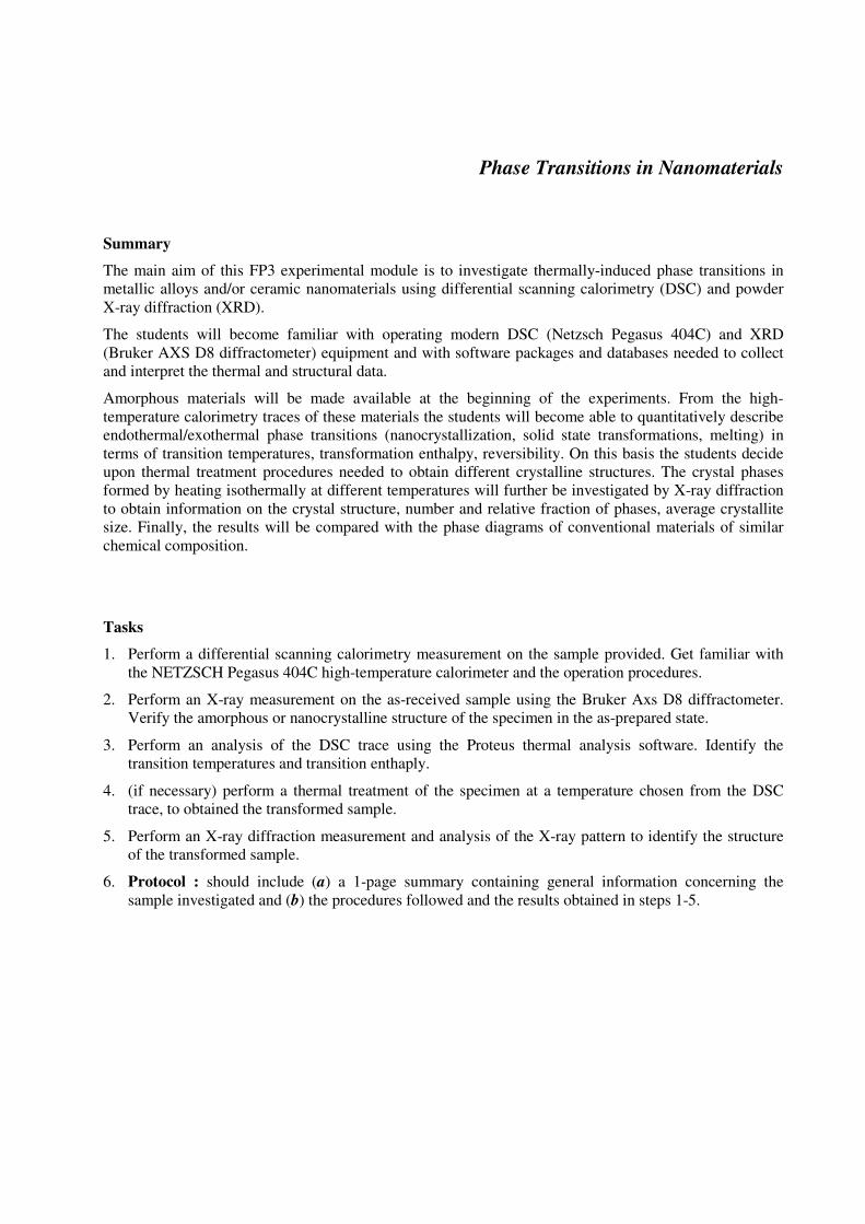
In heat-flux DSC instruments, the difference in energy required to maintain both S and R at the same temperature is a measure of the energy changes in the test specimen S (relative to the inert reference R). The thermocouples are usually not embedded in neither S or R materials. The temperature difference ∆T that develops between S and R is proportional to the heat-flow between the two. In order to detect such small temperature differences, it is essential to ensure that both S and R are exposed to the same temperature programme. The measurements are usually performed under vacuum or inert-gas flow : the flow rate (typically around 40 ml/min.) is maintained contant throughout the experiment.

Notes ( analysis of heat-flow in heat-flux DSC )

The assembly of thermal resistances of the heat-flux DSC system changes with temperature. Nevertheless, DSC instruments may be used in the so-called 'calibrated' mode : the amplification of the DSC signal is then also automatically varied with temperature to maintain a constant calorimetric sensitivity with temperature.

Temperature shifts may occur between the samples (S and R) and thermocouples, since these are not in direct physical contact with the samples. The measured temperature difference ∆Texp is not equal to (TS-TR) where TS and TR are the sample and reference temperatures, respectively. The temperature difference of interest (TS-TR) may be deduced by considering the heat-flow paths in the DSC system (Fig.4).

Fig. 4 Thermal-resistance diagram for a typical heat-flux DSC system.

Greer and Baxter notation :

TSP, TRP = temperature of the sample (SP) and reference (RP) platforms as measured by the thermocouples. TSP is plotted as the abscissa of the measured DSC curve. TF = temperature of the heating block (furnace). RD = thermal resistance between the furnace wall and the SP or RP platforms [C⋅min/J]. RS, RR = thermal resistance between the SP (or reference RP) platform and the sample S (or reference R). CS, CR = heat capacity of the sample S (or reference R) and its container. H = external (imposed) heating rate. ∆TR = temperature difference of the reference platform RP relative to the furnace. ∆TS = temperature difference of the sample platform SP relative to the furnace. ∆TL = temperature difference of the sample S relative to the sample thermocouple.

Then the following equations hold:

∆TR = H⋅RDCR (1)

∆TS = H⋅RDCS (2)

∆T = H⋅RD (CS - CR) (3)

∆TL = H⋅RSCS (4)

∆TS = ∆TR + ∆T (5)

∆TL = RS / RD∆TS (6)

The temperature shift (∆TL) occurs because the thermocouple is not in physical contact with the sample. If a certain phase transition temperature Tx does not vary with the external heating rate H, equation (4) indicates that the plot of the apparent Tx vs. H (with all other parameters fixed), extrapolates to the true transition temperature value Tx0 of Tx at H=0. Therefore, the apparent Tx is the true value Tx0 plus the temperature difference. Note that the plot of apparent Tx versus CS also extrapolates to Tx0 at CS = 0, when H and RS are constant.

Greer procedure: is based on equation (6) and involves the evaluation of RS=RD. (∆TR) is measured for a particular reference (usually an empty pan and lid). An 'empty' heating run is first performed with an empty pan on both the sample and reference platforms. This provides a baseline, from which measurements of ∆T can be carried out. A second run is then performed, with 2 pans on the sample platform and one on the reference platform. The difference between the first and second DSC curves is a measure of (∆TR) as a function of temperature.

This results directly from equations (1) and (3) : for the first 'empty' run, CS=CR and therefore ∆T = 0 (eqn.3), while for the second run CS=2CR, so that ∆T=∆TR (eqn.1). By repeating this procedure for different heating rates, ∆TR can be obtained as a function of heating rate H. To obtain the sample-to-thermocouple temperature difference (∆TL) we use the fact that :

∆TR + ∆T = ∆TS

A series of test measurements is conducted for different heating rates H with a standard sample with known transition temperature Tx (which does not depend on H) mounted in the sample pan and an empty pan mounted on the reference platform. These measurements will provide ∆T(H). Since ∆TR(H) was previously obtained, the above equation will give ∆TS(H). The gradient g1 of the ∆TS vs. H plot equals RDCS (eqn.2).

Another set of experiments (see eqn.4) finally gives a plot of the apparent transition temperature Tx(H) and its extrapolation at H=0 yields the true transition temperature Tx0. The dependence TL vs. H can now be plotted, and its gradient g2 = RSCS (eqn.4) can be obtained. Then :

and the temperature shift ∆TL may be calculated (RS/RD and ∆TR known) using equation (6) for any given reference R and at any heating rate H or CS.

3.3. Calibration of Differential Scanning Calorimeters

Temperature calibration is carried out by running standard materials, usually very pure metals with accurately known melting points. Energy calibration may be carried out by using either known heats of fusion for metals, commonly indium, or known heat capacities. Synthetic sapphire (corundum, or aluminium oxide) is readily available as a heat capacity standard, and the values for this have been accurately determined over a wide temperature range. The absolute accuracy for measurements of heat capacity and transformation enthalpies are more often limited by the lack of appropriate standards, and difficulties in assigning a baseline construction, than by limitations of the instrument itself. DSCs are almost universally calibrated for temperature and enthalpy using the melting temperatures of highly pure metals. Recommended values for the melting temperature (Tm) and heat of fusion (Hf) are given below. Many of these substances will react with standard aluminium crucibles. This may be overcomes by annealing the empty crucible (and lid) air above 400°C in order to build up a protective layer of alumina.

Material Tm (°C) Hf (J/g) Mercury -38.8344 11.469 Gallium 29.7646 79.88 Indium 156.5985 28.62 Tin 231.298 7.170 Bismuth 271.40 53.83 Lead 327.462 23.00 Zinc 419.527 108.6 Aluminium 660.323 398.1

S

D

R

R

g

g=

2

1

References :

G. W. H. Höhne, H. K. Cammenga, W. Eysel, E. Gmelin, W. Hemminger; "The Temperature Calibration of Scanning Calorimeters", Thermochimica Acta, 160 (1990) 1-12

S. M. Sarge, E. Gmelin, G. W. H. Höhne, H. K. Cammenga, W. Hemminger, W. Eysel; "The Caloric Calibration of Scanning Calorimeters", Thermochimica Acta, 247 (1994) 129-168

M. L. Richardson, E. L. Charsley; "Calibration and Standardisation in DSC", in Handbook of Thermal

Analysis and Calorimetry. Vol. 1: Principles and Practice, M. E. Brown (editor), Elsevier Science B.V. (1998)

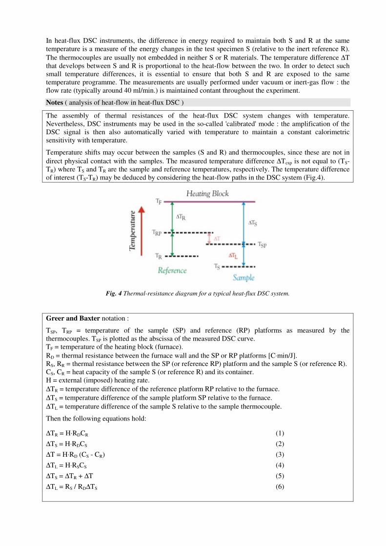
Special choices of the lids (sample holders) must be met for working with calibration substances.

Temperature Calibration

A number of other materials have well defined transition temperatures which make them useful calibration materials (particularly at low temperatures)1

Material Tm (°C)

Toluene -95.01 Cyclohexane (solid-solid) -56.8 Octane -56.8 Decane -29.6 Dodecane -9.6 Water 0.00 Cyclohexane (solid-liquid) 6.7 Diphenyl Ether 26.87 4-Nitrotoluene 51.61

1 D. M. Price; "Temperature Calibration of Differential Scanning Calorimeters", Journal of Thermal Analysis, 45 (1995) 1285-1296

Biphenyl 68.93 Napthalene 80.23 Acetanilide 114.34 Benzoic Acid 122.34 Anisic Acid 183.28 2-Chloroanthraquinone 209.83 Caffeine 236.1 Carbazole 284.52

Organic substances which are liquids at room temperature may be volatile and thus difficult to handle. The solid-solid transitions of ammonium sulphate (-48.8°C) and of ammonium di-hydrogen phosphate (-121.4°C) are particularly useful for low temperature calibration.

Enthalpy Calibration

The energy calibration is carried out by measuring changes in specific heat or in enthalpy of standard specimens for which these quantities are known. The heat balance equation for the heat-flux DSC system can be shown to be as follows (eqn.7) :

dH'/dt refers to the heat evolution of an exothermic transition; the first term on the right side is the area under the DSC peak, after the baseline correction. The second term refers to the actual baseline (this is used in specific heat determinations). The last term takes into account the fact that the evolved heat partially will be consumed by the specimen to heat itself. It does not affect the DSC peak area, but may distort the peak shape.

When dH'/dt = 0, the second term of equation 7 can be used to determine specific heat. The method involves a comparison of the thermal shift (difference) between sample and reference. The system is first calibrated with a sapphire specimen, so that

mH

YqECsapphire

⋅

⋅⋅=

where

m = mass of the specimen E = calibration constant Csapphire = specific heat capacity of sapphire qY = axis range (Js/mm) H = heating rate and Y = difference in Y-axis deflection between sample (or sapphire) and ‘empty’ runs (blank curves) at the temperature of interest.

Enthalpy changes can be determined by measuring the areas under peaks on the DSC curve ∆T vs. time.

Standard method : synthethic sapphire (carborundum, aluminium oxide) is widely used as a calibrant for heat capacity determination. Values of the Cp (in J K-1g-1) at temperature T (in K) of this material are accurately given by the polynomial:

Cp(T) = A + B * T + C * T 2 + D * T 3 + E * T 4 + F * T 5 + G * T 6 + H * T 7

dt

TTd

R

RRCHCC

R

TT

dt

dH RPSP

D

SD

SRS

D

RPSP )()(

' −⋅

+⋅+⋅−+

−=

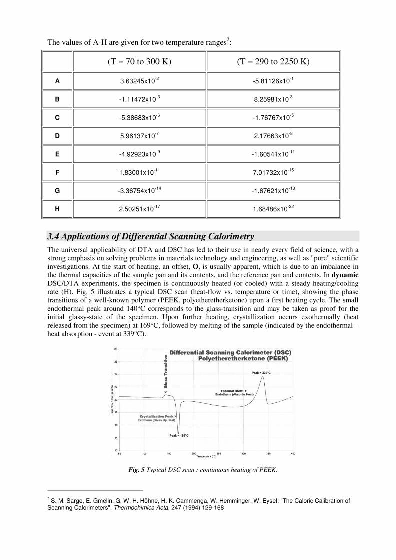
The values of A-H are given for two temperature ranges2:

(T = 70 to 300 K) (T = 290 to 2250 K)

A 3.63245x10-2

-5.81126x10-1

B -1.11472x10-3

8.25981x10-3

C -5.38683x10-6

-1.76767x10-5

D 5.96137x10-7

2.17663x10-8

E -4.92923x10-9

-1.60541x10-11

F 1.83001x10-11

7.01732x10-15

G -3.36754x10-14

-1.67621x10-18

H 2.50251x10-17

1.68486x10-22

3.4 Applications of Differential Scanning Calorimetry

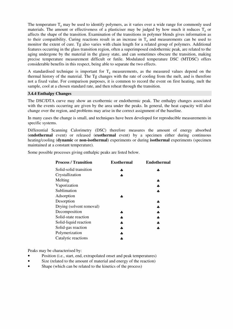
The universal applicability of DTA and DSC has led to their use in nearly every field of science, with a strong emphasis on solving problems in materials technology and engineering, as well as "pure" scientific investigations. At the start of heating, an offset, O, is usually apparent, which is due to an imbalance in the thermal capacities of the sample pan and its contents, and the reference pan and contents. In dynamic DSC/DTA experiments, the specimen is continuously heated (or cooled) with a steady heating/cooling rate (H). Fig. 5 illustrates a typical DSC scan (heat-flow vs. temperature or time), showing the phase transitions of a well-known polymer (PEEK, polyetheretherketone) upon a first heating cycle. The small endothermal peak around 140°C corresponds to the glass-transition and may be taken as proof for the initial glassy-state of the specimen. Upon further heating, crystallization occurs exothermally (heat released from the specimen) at 169°C, followed by melting of the sample (indicated by the endothermal – heat absorption - event at 339°C).

Fig. 5 Typical DSC scan : continuous heating of PEEK.

2 S. M. Sarge, E. Gmelin, G. W. H. Höhne, H. K. Cammenga, W. Hemminger, W. Eysel; "The Caloric Calibration of Scanning Calorimeters", Thermochimica Acta, 247 (1994) 129-168

3.4.1 Heat Capacity Measurements

In the absence of any discrete physical or chemical transformations, the baseline signal is related to the heat capacity of the sample. DSC allows this parameter to be determined with good accuracy over a wide temperature range. The conventional approach is to compare the signal obtained for the sample above that given by an empty pan, with the signal obtained for a standard material, usually sapphire, under the same conditions. Careful experimental technique is required to obtain accurate results, but heat capacities can be routinely measured to accuracies better than ±1%.

The instrument is programmed to heat between the initial and final isothermal stages at Ti and Tf, first with empty pans. A perfect instrument would show no deflection from the isothermal baseline, but this is never the case, and a small signal is given which can be used to correctly measure the deflections given by the sample and sapphire standard when run under precisely the same conditions. The deflections obtained are directly dependent on the heating rate; linearity and reproducibility of the temperature programme are therefore essential for accurate work. The ratio of the deflections is equal to the ratios of the heat capacities of the sample and sapphire.

Other techniques are available for heat capacity measurement by DSC. Accurate data can be obtained in narrow temperature intervals by using a non-equilibrium pulse technique, which is particularly useful when measurements need to be made in a region constrained by adjacent complicating transitions. Less time-consuming experiments than those described above can generate data more rapidly, but at the expense of accuracy and precision, which may be adequate for a given purpose. MTDSC, a recent enhancement of DSC, routinely generates Cp data from a standard experiment, and can in fact measure this in a nominally isothermal condition. The classical method above however is recommended for the best quality results.

3.4.2 First Order Phase Transitions

Thermal analysis techniques have the advantage that only a small amount of material is necessary. This ensures uniform temperature distribution and high resolution. The sample can be encapsulated in an inert atmosphere to prevent oxidation, and low heating rates lead to higher accuracies. The reproducibility of the transition temperature can be checked by heating and cooling through the critical temperature range.

During a first order transformation, a latent heat is evolved, and the transformation obeys the classical Clausius-Clapeyron equation. Second order transitions do not have accompanying latent heats, but like first order changes, can be detected by abrupt variations in compressibility, heat capacity, thermal expansion coefficients and the like. It is these variations that reveal phase transformations using thermal analysis techniques. Because of the sensitivity of liquid-vapour transitions to pressure, additional precautions are called for when testing for boiling points or enthalpy changes. The ambient pressure is required; the peak area no longer corresponds to the latent heat of vaporisation in any simple way. The transition temperature T' is related to the pressure P by the Clausius-Clapeyron equation

ln(P) = L/RT' + C

where L is the molar heat of vaporisation and C is an integration constant. L can be obtained using the Clausius-Clapeyron equation and a set of measured P,T' values, assuming L is independent of temperature, that the volume of the vapour phase far exceeds that of the liquid, and that the vapour behaves as an ideal gas.

Greater care is needed when studying solid-solid transitions where the enthalpy changes are much smaller than those associated with vaporisation. Stored energy in the form of elastic strains and defects can contribute to the energy balance, so that the physical state of the initial solid, and the final state of the product, become important. This stored energy reduces the observed enthalpy change.

3.4.3 Second Order Transitions

The DSC/DTA curve may show a step change, reflecting a change in heat capacity not accompanied by a discrete enthalpy change. The most common example, and a major application area of DSC, is the glass transition (Tg) seen in amorphous polymers. This important region, in which the material changes from a rigid glassy state to a rubber, or very viscous liquid state, may be analysed to give a wealth of information about the material.

The temperature Tg may be used to identify polymers, as it varies over a wide range for commonly used materials. The amount or effectiveness of a plasticiser may be judged by how much it reduces Tg or affects the shape of the transition. Examination of the transitions in polymer blends gives information as to their compatibility. Curing reactions result in an increase in Tg and measurements can be used to monitor the extent of cure. Tg also varies with chain length for a related group of polymers. Additional features occurring in the glass transition region, often a superimposed endothermic peak, are related to the aging undergone by the material in the glassy state, and can sometimes obscure the transition, making precise temperature measurement difficult or futile. Modulated temperature DSC (MTDSC) offers considerable benefits in this respect, being able to separate the two effects.

A standardised technique is important for Tg measurements, as the measured values depend on the thermal history of the material. The Tg changes with the rate of cooling from the melt, and is therefore not a fixed value. For comparison purposes, it is common to record the event on first heating, melt the sample, cool at a chosen standard rate, and then reheat through the transition.

3.4.4 Enthalpy Changes

The DSC/DTA curve may show an exothermic or endothermic peak. The enthalpy changes associated with the events occurring are given by the area under the peaks. In general, the heat capacity will also change over the region, and problems may arise in the correct assignment of the baseline.

In many cases the change is small, and techniques have been developed for reproducible measurements in specific systems.

Differential Scanning Calorimetry (DSC) therefore measures the amount of energy absorbed (endothermal event) or released (exothermal event) by a specimen either during continuous heating/cooling (dynamic or non-isothermal) experiments or during isothermal experiments (specimen maintained at a constant temperature).

Some possible processes giving enthalpic peaks are listed below.

Process / Transition Exothermal Endothermal

Solid-solid transition ♣ ♣ Crystallization ♣ Melting ♣ Vaporization ♣ Sublimation ♣ Adsorption ♣ Desorption ♣ Drying (solvent removal) ♣ Decomposition ♣ ♣ Solid-state reaction ♣ ♣ Solid-liquid reaction ♣ ♣ Solid-gas reaction ♣ ♣ Polymerization ♣ Catalytic reactions ♣

Peaks may be characterised by: • Position (i.e., start, end, extrapolated onset and peak temperatures) • Size (related to the amount of material and energy of the reaction) • Shape (which can be related to the kinetics of the process)

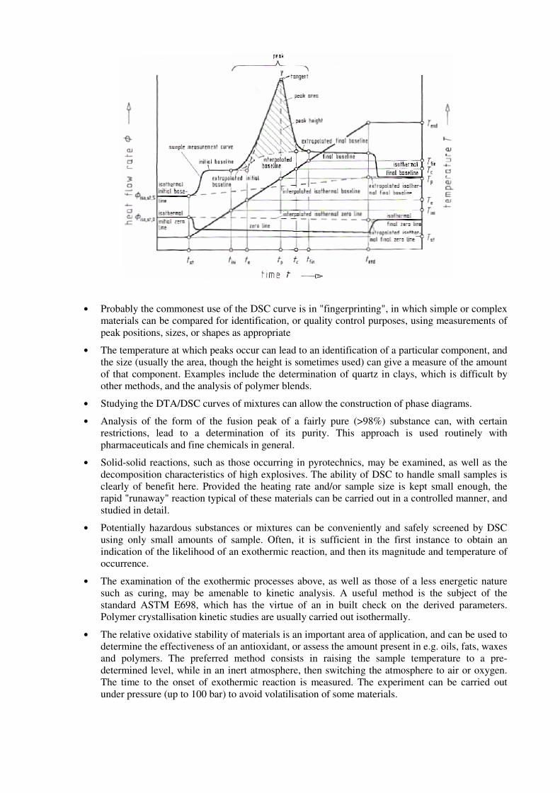
• Probably the commonest use of the DSC curve is in "fingerprinting", in which simple or complex materials can be compared for identification, or quality control purposes, using measurements of peak positions, sizes, or shapes as appropriate

• The temperature at which peaks occur can lead to an identification of a particular component, and the size (usually the area, though the height is sometimes used) can give a measure of the amount of that component. Examples include the determination of quartz in clays, which is difficult by other methods, and the analysis of polymer blends.

• Studying the DTA/DSC curves of mixtures can allow the construction of phase diagrams.

• Analysis of the form of the fusion peak of a fairly pure (>98%) substance can, with certain restrictions, lead to a determination of its purity. This approach is used routinely with pharmaceuticals and fine chemicals in general.

• Solid-solid reactions, such as those occurring in pyrotechnics, may be examined, as well as the decomposition characteristics of high explosives. The ability of DSC to handle small samples is clearly of benefit here. Provided the heating rate and/or sample size is kept small enough, the rapid "runaway" reaction typical of these materials can be carried out in a controlled manner, and studied in detail.

• Potentially hazardous substances or mixtures can be conveniently and safely screened by DSC using only small amounts of sample. Often, it is sufficient in the first instance to obtain an indication of the likelihood of an exothermic reaction, and then its magnitude and temperature of occurrence.

• The examination of the exothermic processes above, as well as those of a less energetic nature such as curing, may be amenable to kinetic analysis. A useful method is the subject of the standard ASTM E698, which has the virtue of an in built check on the derived parameters. Polymer crystallisation kinetic studies are usually carried out isothermally.

• The relative oxidative stability of materials is an important area of application, and can be used to determine the effectiveness of an antioxidant, or assess the amount present in e.g. oils, fats, waxes and polymers. The preferred method consists in raising the sample temperature to a pre-determined level, while in an inert atmosphere, then switching the atmosphere to air or oxygen. The time to the onset of exothermic reaction is measured. The experiment can be carried out under pressure (up to 100 bar) to avoid volatilisation of some materials.

3.5 The NETZSCH 404C Pegasus DSC Instrument 3.4.1 Basic components, technical features & specimen environment

The experiments will be performed using a NETZSCH 404C heat-flux DSC instrument with the following components : • measuring unit : including the high-temperature

SiC oven, sample & reference holders, vacuum and/or inert gas connections

• specimen crucibles : corundum Al2O3 for which Tmax : 1650°C (0.085 cm3).

• thermocouples: type S (Pt10%Rh-Pt).

• NETZSCH TASC/414 T-controller

• furnace power supply

• computer system running the control interface and the Proteus data acquisition and analysis software (Windows NT).

Sample environment : O (oxidizing), R (reducing), I (inert), V (vacuum). The DSC unit operates under vacuum conditions better than 0.0001 mbar, in air or under an inert-gas flow. Allowed gases : nitrogen, argon, helium and oxygen (please note that special rules apply for other gases or gas-mixtures). Temperature range: [30°C (RT) ÷ 1650°C] The accessible temperature range depends also on the thermocouples used, namely :

Type E : (-120° ... 700°C), Chromel-Constantan. Type K : (RT ... 800°C), Chromel-Alumel. Type S : (RT ... 1650°C), Pt10%Rh-Pt. Type B : (150° ...1650°C), Pt30%Rh-Pt6%Rh.

Pans: a variety of sample pans can be used for different purposes. The best quantitative results for polymers are obtained from thin samples crimped flat between the pan and a lid. Hermetically-sealed pans capable of holding a few atmospheres pressure are used for liquids, or when it is necessary to retain volatiles. Very high-pressure seals can be achieved using O-ring or screw-threaded seals. For materials that react with aluminium, or for higher temperatures, pans may be made from stainless steel, inconel, gold, alumina, graphite, silica or platinum.

DSC 404 C Pegasus: List of crucibles Material Tmax/°C Ø Capacity (µl) Remark

Al2O3 1650 6,8 85 pan

Al2O3 1650 6,8 85 high-density material pan

Quartz glass 1100 6,7 85 pan

Duran glass 550 85 pan

Duran glass 550 65 sample tubes, 25 pcs.

Pt/Rh 1600 6,8 85 pan

Pt/Rh 1400 85 pan with Al2O3 liner for reactive material

Al 600 6,0 25/40 set pans / lids, cold-weldable, 100 pcs.

Al 600 6,0 25/40 set pans / lids, cold-weldable, 500 pcs.

Al (99.99) 550 6,7 85 pan

Au 900 6,7 85 pan

Ag 750 6,7 85 pan

ZrO2 1600 6,7 85 pan

Graphite 2000 6,7 85 pan inert atmosphere required!

Cu 700 6,0 40 pan for OIT measurements

Pt/Rh 1500 6,8 85 sample pan

Pressure-tight crucibles with AuCu sealing discs:

Material Tmax/°C Capacity (µl) Remark

CrNi steel gold-plated 500 27 re-usable, max. 100bar, set: 1 crucible / 5 sealings

CrNi steel, gold-plated 500 27 re-usable, max. 100bar, set: 10 crucible/50 sealings

CrNi steel, gold plated 500 100 re-usable, max. 100bar, set: 1 crucible / 5 sealings

Titanium 500 27 re-usable, max. 100bar, set: 1 crucible / 5 sealings

Titanium 500 90 re-usable, max. 100bar, set: 1 crucible / 5 sealings

Crucibles for DTA applications:

Material Tmax/°C Capacity / µl Remark

Al2O3 1650 200 crucible, thin-walled

Al2O3 165 200 crucible, thick-walled

Al2O3 1650 280 crucible

Al2O3 1650 300 crucible

Pt-Ir 1650 300 crucible

Tantalum 1650 300 crucible

Graphite 1650 300 crucible, inert atmosphere required!

Nickel 1300 300 crucible

Stainless steel 1000 300 crucible

Pt-Ir 1650 100 crucible

Al2O3 1650 100 crucible, for mini sample holder

Al (99.5) 550 100 crucible, for mini sample holder

Quartz glass 1000 1300 ampoule

Duran glass 600 1300 ampoule

Gases : typical purge gases are air and nitrogen, though helium is useful for efficient heat transfer and removal of volatiles. Argon is preferred as an inert purge when examining samples that can react with nitrogen. The experiment can also be carried out under vacuum or under high pressure using instruments of the appropriate design. (For more information see Appendix).

3.5.2 Operation Instructions

The goal of a curve correction is the increase of the measurement accuracy by subtracting from the real measurement with sample a measurement without sample that has been carried out under identic measurement conditions (“empty measurement”, “zero line”, “blind measurement”, ”baseline”,

“correction”) to eliminate the behaviour of the empty system. The combinations of sample and correction measurements are provided within the scope of Good laboratory practice (GLP). Sample and correction measurements are permanently stored in the combined “sample + correction”- files, and therefore cannot later be assigned to the analysis of other correction files.

Correction measurement (Baseline)

A correction measurement is defined to determine the instrument behaviour without sample, i.e. with empty crucibles (DSC, TG, STA) or with a length standard (DIL). How to perform a correction (baseline) measurement

1. Open the Measurement Menu by double-clicking the icon. 2. Select in main menu file the sub menu ‘new’ 3. Define your measurement parameters to carry out a sample measurement. Click in the dialog into

‘correction’ to mark the check box. 4. Open a temperature calibration file which fits to your experiment or tcalzero.TMX or

tcalero.TCX. 5. Open a sensitivity calibration file which fits to your experiment or senszero.EXX.

Measurement conditions: The baseline should be carried out under exactly the same conditions as the further sample or calibration measurements Please observe the recommendations for purge gases.

6. Temperature Program: For recording the baseline an acquisition rate is proposed by the software which we experienced in the application labs at NETZSCH-Gerätebau GmbH.

7. Start the measurement This correction measurement can be later opened in order to perform a pure sample measurement or a new correction. A correction measurement can also be used afterwards to add a sample measurement (‘Correction + Sample’). Conversely, it is possible to open a sample measurement in order to add a correction measurement (‘Sample + Correction’). When using the option ‘Sample + Correction’, at the regular end of measurement one obtains the triplet from the sample, correction and combined “sample + correction” measurement, which contains the sample and correction data in one file. Creation of these calibration measurements is subject to several rules for input of the temperature program. The software checks for compliance with these rules during input of the temperature program and prevents errors with appropriate messages. The temperature programs for the correction and sample measurements show the same regime. Sample and baseline data are linked during correction of the combined “sample + correction”- files. Therefore, with respect to time, a correction measurement must never be shorter than the sample measurement planned for the calibration. Only correction measurements with “normal end” may be used for combined “sample + correction”- files. In addition, the sample and correction measurement must have the same, appropriate acquisition rate in every segment.

Correction data file TA measurement system data recorded by a measurement without sample (DSC,TG) or with a calibration standard (DIL/TMA). The actual data on the behaviour of the TA system are stored in a correction data file after the measurement has been completed. In addition, this file contains all information on correction/calibration parameters and the temperature program. Correction data files can be used to execute the next correction measurement, next sample measurement or to create a sample measurement with correction.

Sample measurement

A sample data file is defined to save a measurement without correction. The measurement data are stored in a sample data file after the measurement has been completed. This file contains all information about the sample parameters and the temperature program. How to perform a sample measurement

1. Open the Measurement Menu by double-clicking the icon. 2. Select in main menu file the sub menu ‘new’ 3. Define your measurement parameters to carry out a sample measurement. Click in the dialog into

‘sample’ to mark the check box. 4. Open a temperature calibration file which fits to your experiment or tcalzero.TMX or

tcalero.TCX. 5. Open a sensitivity calibration file which fits to your experiment or senszero.EXX.

Measurement conditions: The baseline should be carried out under exactly the same conditions as the further sample or calibration measurements Please observe the recommendations for purge gases.

6. Temperature Program:

For recording the baseline an acquisition rate is proposed by the software which we experienced in the application labs at NETZSCH-Gerätebau GmbH.

7. Start the measurement

Sample + correction measurement It generates a combined sample + correction data file (suffix D), i.e. that baseline (suffix C, B) and sample (suffix S) data are stored together in one file (suffix D). With such a file, baseline correction (DSC, DTA), buoyancy corrections (TG) or calibrations for dilatometers can be carried out How to link a sample file with an already existing correction data file:

• Double click on the measurement icon in the NETZSCH-TA4 group. • Open a correction data file (suffix C, B). • Select measurement type “sample + correction”. • Define the measurement parameters. • Define the temperature program.

For measurements with one segment one can select lower final temperature for the sample compared with the selected correction measurement. The acquisition rates in both must be identically. Measurements with more than one segment (“multi-segmental”) must have identical temperature limits and acquisition rates for correction and sample measurement. Only the last segment may be shortened if necessary.

• Define the prefix name of the sample data file. Suffix is added according to instrument code.

• Start your measurement. A combined “Sample + correction” file (suffix D) is generated. • Check the selected files in the menu, View Active Files…

How to link measurement data with correction file

• Open a correction data file. • Select measurement type “sample+correction”. • Define the measurement parameters • Define the temperature program. • Define the name of the measurement data file. • Start your measurement. • Check the selected files in the menu, View Active File…

How to link a correction file with an already existing sample data file

• Open a sample data file. • Select measurement type “sample+correction”. • Define the measurement parameters.

Operation Instructions

The instrument operation instructions are provided below as a stepwise check-list :

1. SWITCH-ON [ 60 min. before measurement ] the components in the following order :

- TASC 414/4 Controller - DSC (measuring unit) - PC (start the Proteus software, data-acquisition module) - Thermostat (if available)

2. Verify/Check purge gas supply / Vacuum : • Allowed environment (gases) :

Air N2 Ar (Argon) O2 (Oxygen)

• Vacuum (≤ 10-4 mbar) : measurements under vacuum are also possible, whenever oxidation or the formation of unwanted secondary phases must be avoided.

3. Move furnace into PARK position. 4. Place 2 empty crucibles (with lid) onto the sample carrier. 5. Move furnace a few mm above the sample carrier head & check if sample carrier is centered with

respect to the furnace opening; adjust if necessary (use the front screws; maintain the factory position if possible).

6. Move furnace into the MEASUREMENT position. 7. Adjust expt. conditions (gas, vacuum) : 8. Start the Proteus software package (measurement program). 9. Start the Correction procedure :

- File / New - Test parameters / Measurement Type : Correction (Sample Mass = 0) - Open Temperature Recalibration - Open Sensitivity - Set Temperature Program {link} - Define Filename (*.bdc).

10. Adjustment window : - set threshold values - if necessary, switch the initial conditions ON - START the Correction measurement

11. Sample preparation. 12. After the furnace did cool down, open the furnace. 13. Remove the empty sample-crucible (i.e. in the front of the operator). 14. Weigh the sample using a balance. 15. Fill-in the sample & Insert the sample crucible into the holder. 16. Move the furnace into the MEASUREMENT position. 17. Adjust measuring conditions (gas or vacuum; see Step.10). 18. Start the Sample+Correction measurement :

- Open previously mesured correction file (see Step.9) - Sample Mass = X [mg] (see Step.15) - Test Parameters / Measurement Type : Sample + Correction - Open Temperature Recalibration (confirm presetting) - Open Sensitivity (confirm presetting) - Accept temperature program - Define filename (*.ddc)

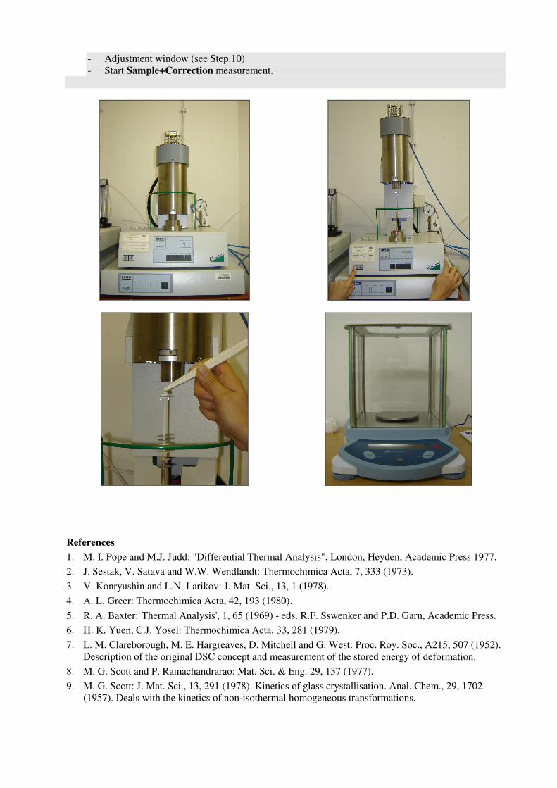
- Adjustment window (see Step.10) - Start Sample+Correction measurement.

References

1. M. I. Pope and M.J. Judd: "Differential Thermal Analysis", London, Heyden, Academic Press 1977.

2. J. Sestak, V. Satava and W.W. Wendlandt: Thermochimica Acta, 7, 333 (1973).

3. V. Konryushin and L.N. Larikov: J. Mat. Sci., 13, 1 (1978).

4. A. L. Greer: Thermochimica Acta, 42, 193 (1980).

5. R. A. Baxter:`Thermal Analysis', 1, 65 (1969) - eds. R.F. Sswenker and P.D. Garn, Academic Press.

6. H. K. Yuen, C.J. Yosel: Thermochimica Acta, 33, 281 (1979).

7. L. M. Clareborough, M. E. Hargreaves, D. Mitchell and G. West: Proc. Roy. Soc., A215, 507 (1952). Description of the original DSC concept and measurement of the stored energy of deformation.

8. M. G. Scott and P. Ramachandrarao: Mat. Sci. & Eng. 29, 137 (1977).

9. M. G. Scott: J. Mat. Sci., 13, 291 (1978). Kinetics of glass crystallisation. Anal. Chem., 29, 1702 (1957). Deals with the kinetics of non-isothermal homogeneous transformations.

Appendix : Temperature calibration

The accuracy of temperature measurements of made with thermal analysis instruments can be affected by changes in the apparatus. Some of the reasons for these deviations are long-time drift of electronic amplifiers and the aging process of thermocouples. The dynamics of these changes are primarily dependent on the number of measurements and the measurement conditions.

For this, calibration materials for which the transformation temperatures are known with sufficient accuracy must be measured in an experimental run independent of the actual measurement and then saved as the calibration curve.

The magnetic features of some substances (for example Ni, Fe) change reproducibly their magnetic features at defined temperatures and due to this fact they can therefore be used for temperature calibration. We would like to point out that the transition temperature of ICTA and NBS materials are experimental mean values. This means that even a temperature calibration of a thermo balance, rundone by the using of magnetic reference substances, may not be completely reliable and can be afflicted with some uncertainties.

In accordance with DIN 51 006 and ASTM E 914, the changes in the magnetic characteristics of selected substances at defined temperatures (Curie point) are used for the temperature calibration of thermo balances. The extrapolated end temperatures of the TG steps which occur are characteristic.

The sections Measurement and Analysis require the input of temperature calibration data.

The ZERO calibration curve TCALZERO is stored prior to delivery of before the instrument is shipped.

ZERO calibration curve = the known transformation temperatures and the measured values are equal, the three coefficients are zero. The temperature calibration is inactive. TCALZERO.TMX Use this file to record and save not recalibrated raw data. or TCALZERO.TCX The file is write-protected and therefore cannot be edited. How to perform measurements of temperature calibrations

1. Prepare the necessary calibration substances (select a calibration set). The materials contained I the calibration sets

-50°C…750°C: 6.223.5-91.1

Room temp. … 900°C: 6.223.5-91.2

Room temp. …1500°C: 6.22.3.5-91.3 are intended solely for use the laboratory. Please use that calibration set which is applicable for the temperature range of your measurement.

2. Open the Measurement Menu by double-clicking the icon. 3. Select in main menu file the sub menu ‘new’. 4. Define your measurement parameters to carry out a sample measurement. 5. Open the temperature calibration file tcalzero.TCX and nothing else. 6. Temperature Program:

Each calibration material must be heated two or three times over the effect to be observed (melting). The two or three required heatings are to be carried out with the same sample either within the temperature program (with appropriate cooling phase) or in separate heating phases. For recording the melting peaks a data acquisition rate of at least 6 to 8 points/K should be used. In general, the end temperature of the heating phase should not exceed the corresponding melting peak by more than 10 to 20 K. In the cooling phases, a temperature of approx. 100°C below the corresponding transition point should be achieved in order to guarantee complete crystallization. The measurement curves for the second and the third heating are always evaluated. (The first heating represents the first melting of the material and cannot always be used!).

7. In the Diagnosis Menu (Adjustment Test) the temperature calibration is inactive in the status line. (no point display!)

8. Start the measurement Repeat steps 2 to 8 with all materials of the calibration set. Measurement conditions: The temperature calibration should be carried out under exactly the same conditions as the corresponding sample measurements. This is valid for temperature calibration carried out using TCALZERO to start the calibration measurement. Please observe the recommendations for purge gases. The temperature data saved during the measurement is then the uncalibrated, raw data. The physical or chemical reaction of the sample material must be analyzed with the onset temperature in program part analysis. How to proceed in analysis

1. Start the Proteus evaluation 2. Open the measurement that calibration substance you will use for the temperature calibration. 3. Carry out a separation of a multisegment measurement under Segment Selection 4. Change to temperature scaling. 5. Click on the measuring curve and define the onset as characteristic result. 6. Average the onset values of one run indifferent segments. 7. Note down the averaged values of the different calibration substances. 8. Start the tool temperature calibration in the Menu | Extra : Temp.calib.

8.1 Select File | New 8.2 Enter the found values in the column Temp.exp/°C of the table. 8.3 If all calibration substances are entered, get the new calibration curve calculation. 8.4 Clicking on the button get displayed the graphic. 8.5 If you quit the range of temperature calibration with OK and exit, you are asked to store

with a name you like. 8.6 With these measured, calculated, noted and entered mean values a temperature calibration

curve is created and stored for the selected measurement conditions, which you can use in future baseline and sample measurement instead of TCALZERO or an old calibration

curve until a new curve is created.

In connection with the calibration of your instrument, please observe the appropriate safety regulations when handling chemicals. These are listed in the corresponding safety specification sheets. In general, suitable protection should be on hand for skin (gloves) and eyes (safety glasses).

Please always observe the maximum operating temperatures of your system components (furnace,

sample carrier, thermocouple, etc.).

Metal cannot be used in Pt crucibles due to the formation of alloys. Therefore, the calibration set 6.223.5-

91.2 includes eight organic and inorganic substances, recognized of calibration purposes, which cover the temperature range from room temperature to approx. 900°C.

The calibration should be carried out on a routine basis. The temperature calibration serves to check the measured temperature signal. It should be carried out at least once a year for each sample thermocouple (i.e. for each sample carrier) and is dependent on the measurement conditions (crucible, atmosphere, flow rate, heating rate, sample weight). In between the completely new calibration, it is recommended that the valid calibration curve be checked with one or two selected substances at least every two months. Additional checks are necessary if there are any indications of sample carrier contamination. Attention: Nickel displays a marked tendency to oxidize at higher temperatures. Therefore, in order to obtain reproducible temperature values, it is advisable that the nickel be melted in a gas atmosphere totally absent of air. A sufficiently high weight should also be selected, such that the surface area of the sample is small in comparison to the volume. In the presence (of traces) of oxygen, the melting temperature is reduced by up to 15 K. The melting point of silver shifts to lower temperature values with the increase of oxygen partial pressure. As a result, the extrapolated onset temperature in static air

atmosphere is lower than that given in the literature. Therefore, two temperatures are listed for silver. In inert gas atmosphere, Zinc starts to evaporate at 500°C. Therefore it is recommended that the material be cooled down immediately after passing the melting peak. Due to the fact, that Zinc starts to oxidize above 225°C, the sample can be used only for one calibration run (two or three heatings). Please be extremely careful when handling Mercury because it is poisonous when inhaled (even at room temperature). Mercury should not be heated above room temperature. Please be careful when handling inorganic salts. Concerning biphenyl and benzoic acid, the melting is used for calibration; all other materials show polymorphous transformations in the temperature ranges of interest. Benzoic acid begins to sublimate after melting. Therefore it is recommended that the material be cooled down immediately after passing the melting peak. Cesium chloride should be weighed prior to each measurement (i.e. for every heating).

Appendix : Spülgase Informationen über die Möglichkeiten der Anwendung von Gasen können der einschlägigen Fachliteratur entnommen oder bei den Herstellern und Vertreibern von Gasen angefordert werden. Nachfolgend ist eine Auswahl von Spülgasen einschließlich der ihre Verwendung einschränkenden Eigenschaften aufgeführt. Die Liste erhebt keinen Anspruch auf Vollständigkeit. Helium (He) chemisch inert (Edelgas) keine sicherheitstechnischen Einschränkungen Argon (Ar) chemisch inert (Edelgas) erstickend wirkend keine sicherheitstechnischen Einschränkungen bei Tieftemperaturversuchen sollte Argon nicht verwendet werden Stickstoff (N2) weitgehend inert erstickend wirkend keine sicherheitstechnischen Einschränkungen, jedoch sind Reaktionen mit der Probe im Hochtemperaturbereich möglich Luft oxidierend keine sicherheitstechnischen Einschränkungen, jedoch sind Reaktionen mit der Probe möglich Einsatzbereich oberhalb Raumtemperatur, maximale Einsatztemperatur wird festgelegt durch Ofenmaterial, Probentyp, Tiegelmaterial bei Einsatz im Tieftemperaturbereich (LN2) kann es zur Verflüssigung des Sauerstoffs kommen Sauerstoff brandfördernd (darf nicht mit Fetten oder Ölen in Kontakt kommen!) keine sicherheitstechnischen Einschränkungen, jedoch sind Reaktionen mit der Probe möglich

Einsatzbereich oberhalb Raumtemperatur, maximale Einsatztemperatur wird festgelegt durch Ofenmaterial, Probentyp, Tiegelmaterial bei Einsatz im Tieftemperaturbereich (LN2) kann es zur Verflüssigung des Sauerstoffs kommen Kohlendioxid (CO2) ungiftig (MAK-Wert 5000vpm) nicht brennbar Verwendung oberhalb Raumtemperatur möglich Wasserstoff (H2) brennbar Das Gerät ist nicht zur Benutzung unter Wasserstoffatmosphäre bestimmt und geeignet. Bei der Durchführung entsprechender Experimente kann es zur Bildung von explosionsfähigen Gemischen im Inneren des Systems kommen Ammoniak (NH3) giftig (MAK-Wert 50 vpm)

brennbar bei Sauerstoffzutritt Explosionsgefahr! Das Gerät ist nicht zur Benutzung unter Ammoniakatmosphäre bestimmt und geeignet. Bei der Durchführung entsprechender Experimente kann es zur Bildung von explosionsfähigen Gemischen im Inneren des Systems kommen. Korrosive Wirkung auf Dichtungen möglich! Kohlenmonoxid giftig (CO) (MAK-Wert- 30vpm) bei Sauerstoffzutritt Explosionsgefahr! Das Gerät ist nicht zur Benutzung unter Kohlenmonoxidatmosphäre bestimmt und geeignet. Bei der Durchführung entsprechender Experimente kann es zur Bildung von explosionsfähigen Gemischen im Inneren des Systems kommen. Schwefelwasserstoff giftig (H2S) (MAK-Wert 10vpm) brennbar korrosiv Verwendung von Schwefelwasserstoff aus sicherheitstechnischen Gründen verboten! Andere Das Gerät ist nicht zur Benutzung unter Atmosphären reduzierende reduzierender Gase oder Gasgemische bestimmt und geeignet. Gase oder Bei der Durchführung entsprechender Experimente kann Gasgemische es zur Bildung von explosionsfähigen Gemischen im Inneren des Systems kommen. Chlor (Cl2) sehr giftig (MAK-Wert 0,5 vpm) nicht brennbar, brandfördend, korrosiv, ätzend Verwendung von Chlor ist aus sicherheitstechnischen Gründen verboten! Chlorwasserstoff giftig (HCl) (MAK-Wert 5vpm) nicht brennbar, korrosiv, ätzend Verwendung von Chlorwasserstoff aus sicherheitstechnischen Gründen verboten! Schwefeldioxid giftig (SO2) (MAK-Wert 2vpm) nicht brennbar, korrosiv Verwendung von Schwefeldioxid aus sicherheitstechnischen Gründen verboten! Schwefelwasserstoff giftig (H2S) (MAK-Wert 10vpm) brennbar, korrosiv Verwendung von Schwefelwasserstoff aus sicherheitstechnischen Gründen verboten! Fluor (F2) sehr giftig (MAK-Wert 0,1 vpm) brandfördernd, korrosiv, ätzend Verwendung von Fluor aus sicherheitstechnischen Gründen verboten! Fluorwasserstoff sehr giftig (HF) (MAK-Wert 3 vpm)

stark ätzend, korrosiv Verwendung von Fluorwasserstoff aus sicherheitstechnischen Gründen verboten!

Gasförmige Verwendung gasförmiger Kohlenwasserstoffe aus Kohlenwasserstoffe sicherheitstechnischen Gründen verboten! Gase oder Gasgemische müssen nach dem Austritt aus dem Messteil unbedingt über einen Abzug abgeleitet werden. Das Messteil muss nach Beendigung der Messung ausreichend mit Inertgas gespült werden.