fortran - background · 2.3 gnu compiler (gfortran) 3. a simple program 4. basic elements of...

Fortran Part I - 1 - David Apsley

FORTRAN Last revision 13/12/2018

PART I – INTRODUCTION TO FORTRAN

1. Fortran Background 1.1 Fortran history and standards

1.2 Source code and executable code

1.3 Fortran Compilers

2. Creating and Compiling Fortran Code

2.1 NAG compiler – using the FBuilder IDE

2.2 NAG compiler – using the command window

2.3 Gnu compiler (gfortran)

3. A Simple Program

4. Basic Elements of Fortran 4.1 Variable names

4.2 Data types

4.3 Declaration of variables

4.4 Numeric operators and expressions

4.5 Character operators

4.6 Logical operators and expressions

4.7 Line discipline

4.8 Miscellaneous remarks

5. Repetition: do and do while

5.1 Types of do loop

5.2 Deterministic do loops

5.3 Non-deterministic do loops

5.4 Cycle and exit

5.5 Nested do loops

5.6 Non-integer steps

5.7 Implied do loops

6. Decision-Making: if and select

6.1 The if construct

6.2 The select construct

7. Arrays 7.1 One-dimensional arrays (vectors)

7.2 Array declaration

7.3 Dynamic arrays

7.4 Array input/output and implied do loops

7.5 Element-by-element operations

7.6 Matrices and higher-dimension arrays

7.7 Terminology

7.8 Array initialisation

7.9 Array expressions

7.10 Array sections

7.11 The where construct

7.12 Array-handling functions

8. Text Handling 8.1 Character constants and variables

8.2 Character assignment

8.3 Character operators

8.4 Character substrings

8.5 Comparing and ordering

8.6 Character-handling functions

9. Functions and Subroutines

9.1 Intrinsic procedures

9.2 Program units

9.3 Subprogram arguments

9.4 The save attribute

9.5 Array arguments

9.6 Character arguments

10. Input and Output

10.1 read and write

10.2 Input/output with files

10.3 Formatted write

10.4 The read statement

10.5 Repositioning input files

10.6 Additional specifiers

10.7 Internal files – characters

11. Modules 11.1 Sharing variables

11.2 Internal functions

11.3 Compiling programs with modules

Recommended Books

Hahn, B.D., 1994, Fortran 90 For Scientists and Engineers, Arnold

Chapman, S.J., 2007, Fortran 95/2003 For Scientists and Engineers (3rd Ed.), McGraw-Hill

Chapman, S.J., 2017, Fortran For Scientists and Engineers (4th Ed.), McGraw-Hill – updated version, very expensive.

Metcalf, M., Reid, J. and Cohen, M., 2018, Modern Fortran Explained, OUP, outstanding and up-to-date definitive text, but not

for beginners.

Fortran - 2 - David Apsley

1. FORTRAN BACKGROUND

1.1 Fortran History and Standards

Fortran (FORmula TRANslation) was the first high-level programming language. It was devised by John Bachus in 1953. The

first Fortran compiler was produced in 1957.

Fortran is highly standardised, making it extremely portable (able to run on a wide range of platforms). It has passed through a

sequence of international standards, those in bold below being the most important:

Fortran 66 – original ANSI standard (accepted 1972!);

Fortran 77 – ANSI X3.9-1978 – structured programming;

Fortran 90 – ISO/IEC 1539:1991 – array operations, dynamic arrays, modules, derived data types;

Fortran 95 – ISO/IEC 1539-1: 1997 – minor revision;

Fortran 2003 – ISO/IEC 1539-1:2004(E) –object-oriented programming; interoperability with C;

Fortran 2008 – ISO/IEC 1539-1:2010 – coarrays (parallel programming)

Fortran “2018” – imminent! See https://wg5-fortran.org/f2018.html

Fortran is widely-used in high-performance computing (HPC), where its ability to run code in parallel on a large number of

processors make it popular for computationally-demanding tasks in science and engineering.

1.2 Source Code and Executable Code

In all high-level languages (Fortran, C++, Java, Python, …) programmes are written in source code. This is a human-readable set

of instructions that can be created or modified on any computer with any text editor. Filetypes identify the programming

language; e.g.

Fortran files typically have filetypes .f90 or .f95

C++ files typically have filetype .cpp

The job of the compiler is to turn this into machine-readable executable code.

Under Windows, executable files have filetype .exe

In this course the programs are very simple and most will be contained in a single file. However:

in real engineering problems, code is often contained in many separate source files;

producing executable code is actually a two-stage process:

– compiling converts each individual source file into intermediate object code;

– linking combines all the object files with additional library routines to create an executable program.

Most Fortran code consist of multiple subprograms or procedures, all performing specific, independent tasks. These may be in

one file or in separate files. The latter arrangement allows related routines to be collected together and used in different

applications. Modern Fortran makes extensive use of modules for this.

1.3 Fortran Compilers

The primary Fortran compiler in the University teaching clusters is the NAG fortran compiler (nagfor), which has an

associated integrated development environment (Fortran Builder). However, many other Fortran compilers exist and your

programs should be able to use any of them. The Intel Fortran compiler (ifort) is also available within the University, but

there are only a small number of licences for PCs.

Other compilers are available to researchers on the Manchester Computational Shared Facility (CSF).

There are many other Fortran compilers. Free Fortran compilers for PCs include:

Gnu Fortran (gfortran) http://gcc.gnu.org/wiki/GFortran

Silverfrost FTN95 http://www.silverfrost.com/ (Fortran 95, on Windows only)

The web page for this course includes a list of Fortran compilers, including some online.

https://wg5-fortran.org/f2018.html

http://gcc.gnu.org/wiki/GFortran

http://www.silverfrost.com/32/ftn95/ftn95_personal_edition.asp


2. Creating and Compiling Fortran Code

You may create, edit, compile and run a Fortran program either:

from the command line;

in an Integrated Development Environment (IDE).

You can create Fortran source code with any text editor: e.g. notepad in Windows, vim in linux, or any more advanced editor.

Many people (but not I) like the bells and whistles that come with their favourite IDE.

The traditional way to start programming in a new language is to create, compile and run a simple program to write “Hello,

world!”. Use an editor or an IDE to create the following file and call it prog1.f90.

program hello

print *, "Hello, world!"

end program hello

Compile and run this code using any of the methods below. Note that all compilers will have their own particular set of options

regarding the naming of files, syntax restrictions and checking, optimisation, linking run-time libraries etc. For these you must

consult individual compiler documentation.

2.1 NAG Fortran – Using the FBuilder IDE

Start the FBuilder IDE from the NAG program group on the Windows Start menu.

Either type in the Fortran source code using the built-in editor (File > New), or open a previously-created source file (File

> Open). Whichever you do, make sure that it is saved with a .f90 or .f95 extension.

Run it from the “Execute” icon on the toolbar. This will automatically save and compile (if necessary), then run your program.

An executable file called prog1.exe will appear in the same folder as the source file.

FBuilder does many things that facilitate code development, like colour-coding syntax and allowing you to save, compile or

run at the press of a button. It also creates many unnecessary files in the process and makes setting compiler options complicated,

so I personally prefer the command-line approach below.

Within FBuilder, help (for both Fortran language and compiler) is available from a pull-down menu.

2.2 NAG Fortran – Using the Command Line

Open a command window. (In the University clusters, to set the PATH environment variable to find the compiler you may have

to launch the command window from the NAG program group on the Start menu).

Navigate to any suitable folder; e.g. cd \work

Create (and then save) the source code: notepad prog1.f90

Compile the code by entering

nagfor prog1.f90 (which creates an executable a.exe)

or:

nagfor –o prog1.exe prog1.f90 (to create an executable prog1.exe)

Run the executable (assuming you have called it prog1.exe as above) by typing its name:

prog1.exe

or, since the system runs .exe files automatically, just:

prog1

Help (on compiler options only) is available from the command line: nagfor –help

You may like to experiment with some of the non-default options: for example, those that assist with debugging or doing run-

time checks.


2.3 Gnu Compiler (gfortran)

This is actually my favourite compiler. It is part of the wider Gnu compiler collection (GCC), which also includes compilers for

C++ and other languages. It can be downloaded either as a stand-alone, as part of the MinGW collection (see the link from this

course’s website), or bundled with an IDE like Code::Blocks (downloadable from http://www.codeblocks.org/).

To compile a single file from the Windows command line just type

gfortran prog1.f90 (which creates an executable a.exe)

More advanced options include:

gfortran -o prog1.exe prog1.f90 (to create an executable prog1.exe)

gfortran –Wall -pedantic prog1.f90 (to increase the error-checking and warnings)

The executable program can be run in the command window simply by typing its name (with or without the .exe extension).

Alternatively, you can edit, compile and run files all from the comfort of an IDE such as Code::Blocks.

http://www.codeblocks.org/


3. A SIMPLE PROGRAM

Example. Quadratic-equation solver (real roots).

The well-known solutions of the quadratic equation

𝐴𝑥2 + 𝐵𝑥 + 𝐶 = 0 are

𝑥 =−𝐵 ± √𝐵2 − 4𝐴𝐶

2𝐴

The roots are real if and only if the discriminant 𝐵2 − 4𝐴𝐶 is greater than or equal to zero.

A program which asks for the coefficients and then outputs the real roots might look like the following.

program roots

! Program solves the quadratic equation ax**2+bx+c=0

implicit none

real a, b, c ! Declare variables

real discriminant, root1, root2

print *, "Input a, b, c" ! Request coefficients

read *, a, b, c

discriminant = b ** 2 - 4.0 * a * c ! Calculate discriminant

if ( discriminant < 0.0 ) then

print *, "No real roots"

else

! calculate roots

root1 = ( -b + sqrt( discriminant ) ) / ( 2.0 * a )

root2 = ( -b - sqrt( discriminant ) ) / ( 2.0 * a )

print *, "Roots are ", root1, root2 ! output roots

end if

end program roots

This example illustrates many of the features of Fortran (or, indeed, other programming languages).

(1) Statements

Fortran source code consists of a series of statements. The usual use is one per line (interspersed with blank lines for clarity).

However, we shall see later that it is possible to have more than one statement per line and for one statement to run over several

lines.

Lines may be up to 132 characters long.

(2) Comments

The exclamation mark (!) signifies that everything after it on that line is a comment (i.e. ignored by the compiler, but there for

your information). Use your common sense.

(3) Constants

Elements whose values don’t change are termed constants. Here, 2.0 and 4.0 are numerical constants. The presence of the

decimal point indicates that they are of real type. We shall discuss the difference between real and integer types later.

(4) Variables

Entities whose values can change are termed variables. Each has a name that is, basically, a symbolic label associated with a

specific location in memory. To make the code more readable, names should be descriptive and meaningful; e.g.

discriminant in the above example.


All the variables in the above example have been declared of type real (i.e. floating-point numbers). Other types (integer,

complex, character, logical, …) will be introduced later, where we will also explain the implicit none statement.

Variables are declared when memory is set aside for them by specifying their type, and defined when some value is assigned to

them.

(5) Operators

Fortran makes use of the usual binary numerical operators +, -, * and / for addition, subtraction, multiplication and division,

respectively. ** indicates exponentiation (“to the power of”).

Note that “=” is an assignment operation, not a mathematical equality. Read it as “becomes”. It is perfectly legitimate (and,

indeed, common practice) to write statements like n = n + 1

meaning, effectively, “add 1 to variable n”.

(6) Intrinsic Functions

The Fortran standard provides some intrinsic (that is, built-in) functions to perform important mathematical functions. The

square-root function sqrt is used in the example above. Others mathematical ones include cos, sin, log, exp, tanh. A list

of useful mathematical intrinsic functions is given in Appendix A4.

Note that, in common with all other serious programming languages, the trigonometric functions sin, cos, etc. expect their

arguments to be in radians.

(7) Simple Input/Output

Simple list-directed input and output is achieved by the statements

read *, list

print *, list

respectively. The contents are determined by what is in list and the *’s indicate that the input is from the keyboard and that the

computer should decide how to format the output. Data is read from the standard input device (usually the keyboard) and output

to the standard output device (usually the screen). In Section 10 it will be shown how to read from and write to files and how to

produce formatted output.

(8) Decision-making

All programming languages have some facility for decision-making: doing one thing if some condition is true and (optionally)

doing something else if it is not. The particular form used here is

if ( some condition ) then

[ do something ] else

[ do something else ] end if

We shall encounter various other forms of the if construct in Section 6.

(9) The program and end program statements

Every Fortran program has one and only one main program. We shall see later that it can have many subprograms (subroutines

or functions). The main program has the structure

program name

[ declaration statements ]

[ executable statements ]

end program name


(10) Cases and Spaces

Except within character contexts, Fortran is completely case-insensitive. Everything may be written in upper case, lower case or

a combination of both, and we can refer to the same variable as ROOT1 and root1 within the same program unit. Warning: this

is a very bad habit to get into, however, because it is not true in major programming languages like C, C++ and Java.

Very old versions of Fortran required you to write programs in upper case, start comments with a c in column 1, and start

executable statements in column 6. These ceased to be requirements many decades ago (although many ill-informed denigrators

of Fortran seem to be living in the prehistoric era when they were! They can probably tell you about punched cards, too!)

Spaces are generally valid everywhere except in the middle of names and keywords. As with comments, they should be used to

aid clarity.

Indentation is optional but highly recommended, because it makes it much easier to understand a program’s structure. It is

common to indent a program’s contents by 3 or 4 spaces from its header and end statements, and to further indent the statements

contained within, for example, if constructs or do loops by a similar amount. Be consistent with the amount of indentation.

(Because different editors have different tab settings – and they are often ridiculously large – I firmly recommend that you use

spaces rather than tabs.)

(11) Running the Program.

Follow the instructions in Section 2 to compile and link the program.

Run it by entering its name at the command prompt or from within an IDE. It will ask you for the three coefficients a, b and c.

Try a = 1, b = 3, c = 2 (i.e. 0232 xx ). The roots should be –1 and –2. You can input the numbers as

1 3 2 [enter]

or

1,3,2 [enter]

or even

1 [enter]

3 [enter]

2 [enter]

Now try the combinations

a = 1, b = –5, c = 6

a = 1, b = –5, c = 10 (What are the roots of the quadratic equation in this case?)


4. BASIC ELEMENTS OF FORTRAN

4.1 Variable Names

A name is a symbolic link to a location in memory. A variable is a memory location whose value may be changed during

execution. Names must:

have between 1 and 63 alphanumeric characters (alphabet, digits and underscore);

start with a letter.

It is possible – but unwise – to use a Fortran keyword or standard intrinsic function as a variable name. However, this will then

prevent you from using the corresponding intrinsic function. Tempting names that should be avoided in this respect include:

count, len, product, range, scale, size, sum, tiny.

The following are valid (if unlikely) variable names: Manchester_United

as_easy_as_123

The following are not:

Romeo+Juliet (+ is not allowed)

999help (starts with a number)

Hello! (! would be treated as a comment, not part of the variable name)

4.2 Data Types

In Fortran there are 5 intrinsic (i.e. built-in) data types:

integer

real

complex

character

logical

The first three are the numeric types. The last two are non-numeric types.

It is also possible to have derived types and pointers. Both of these are highly desirable in a modern programming language (and

are similar to features in C++). These are described in the advanced section of the course.

Integer constants are whole numbers, without a decimal point, e.g.

100 +17 –444 0 666

They are stored exactly, but their range is limited: typically –2n-1 to 2n-1–1, where n is either 16 (for 2-byte integers) or 32 (for 4-

byte integers – the default for most compilers). It is possible to change the default range using the kind type parameter (see

later).

Real constants have a decimal point and may be entered as either

fixed point, e.g. 412.2

floating point, e.g. 4.122e+02

Real constants are stored in exponential form in memory, no matter how they are entered. They are accurate only to a finite

machine precision (which, again, can be changed using the kind type parameter).

Complex constants consist of paired real numbers, corresponding to real and imaginary parts. e.g. (2.0,3.0) corresponds to

2 + 3i.

Character constants consist of strings of characters enclosed by a pair of delimiters, which may be either single (') or double

(") quotes; e.g.

'This is a string'

"School of Mechanical, Aerospace and Civil Engineering"

The delimiters themselves are not part of the string.

Logical constants may be either .true. or .false.


4.3 Declaration of Variables

Type

Variables should be declared (that is, have their data type defined and memory set aside for them) before any executable

statements. This is achieved by a type declaration statement of the form, e.g., integer num

real x

complex z

logical answer

character letter

More than one variable can be declared in each statement. e.g. integer i, j, k

Initialisation

If desired, variables can be initialised in their type-declaration statement. In this case a double colon (::) separator must be used.

Thus, the above examples might become: integer :: num = 20

real :: x = 0.05

complex :: z = ( 0.0, 1.0 )

logical :: answer = .true.

character :: letter = 'A'

Variables can also be initialised with a data statement; e.g.

data num, x, z, answer, letter / 20, 0.05, ( 0.0, 1.0 ), .true., 'A' /

The data statement must be placed before any executable statements.

Attributes

Various attributes may be specified for variables in their type-declaration statements. One such is parameter. A variable

declared with this attribute may not have its value changed within the program unit. It is often used to emphasise key physical or

mathematical constants; e.g. real, parameter :: gravity = 9.81

Other attributes will be encountered later and there is a list of them in the Appendix. Note that the double colon separator (::)

must be used when attributes are specified or variables are initialised – it is optional otherwise.

Precision and “Kind”

By default, in the particular Fortran implementation in the University clusters a variable declared by, e.g., real x

will occupy 4 bytes of computer memory and will be inaccurate in the sixth significant figure. The accuracy can be increased by

replacing this type statement by the often-used, but now deprecated, double precision x

with the floating-point variable now requiring twice as many bytes of memory.

Unfortunately, the number of bytes with which real and double precision floating-point numbers are stored is not

standard and varies between implementations. Similarly, whether an integer is stored using 4 or 8 bytes affects the largest

number that can be represented exactly. Sometimes these issues of accuracy and range may lead to different results on different

computers. Better portability can be assured using kind parameters

Although it doesn’t solve the portability problem, I avoid the double precision statement by using:

integer, parameter :: rkind = kind( 1.0d0 )

followed by declarations for all floating-point variables like: real(kind=rkind) x

To switch to single precision for all floating-point variables just replace 1.0d0 by 1.0 in the first statement.

Intrinsic functions which allow you to determine the kind parameter for different types are


selected_char_kind( name )

selected_int_kind( range )

selected_real_kind( precision, range )

Look them up if you need them.

Historical Baggage – Implicit Typing.

Unless a variable was explicitly typed (integer, real etc.), older versions of Fortran implicitly assumed a type for a variable

depending on the first letter of its name. If not explicitly declared, a variable whose name started with one of the letters i-o was

assumed to be an integer; otherwise it was assumed to be real. (Hence the appalling Fortran joke: “God is real, unless declared

integer”!).

To allow older code to run, Fortran has to permit implicit typing. However, it is very bad programming practice (leading to major

errors if you mis-type a variable: e.g. angel instead of angle), and it is highly advisable to:

use a type declaration for all variables;

put the implicit none statement at the start of all program units (this turns off implied typing and the compilation

will fail with an error warning if you have forgotten to declare the type of a variable).

4.4 Numeric Operators and Expressions

A numeric expression is a formula combining constants, variables and functions using the numeric intrinsic operators given in

the following table. The precedence is exactly the same as the normal rules of algebra.

operator meaning precedence (1 = highest)

** exponentiation (xy) 1

* multiplication (xy) 2

/ division (x/y) 2

+ addition (x+y) or unary plus (+x) 3

- subtraction (x–y) or unary minus (–x) 3

Operators with two operands are called binary operators. Those with one operand are called unary operators.

Precedence

Expressions are evaluated in exactly the same order as in normal mathematics: highest precedence first, then (usually) left to

right. Brackets ( ), which have highest precedence of all, can be used to override this. e.g.

1 + 2 * 3 evaluates as 1 + (2 3) or 7

10.0 / 2.0 * 5.0 evaluates as (10.0 / 2.0) 5.0 or 25.0

5.0 * 2.0 ** 3 evaluates as 5.0 (2.03) or 40.0

Repeated exponentiation is the single exception to the left-to-right rule for equal precedence:

a ** b ** c evaluates as cba

Type Coercion

When a binary operator has operands of different type, the weaker (usually integer) type is coerced (i.e. converted) to the

stronger (usually real) type and the result is of the stronger type. e.g.

3 / 10.0 3.0 / 10.0 0.3

*** WARNING *** A common source of difficulty to beginners is integer division. This is not unique to Fortran: it works

exactly the same in many programming languages, including C, C++ and Java. If an integer is divided by an integer then the

result must be an integer and is obtained by truncation towards zero. Thus, in the above example, if we had written 3/10

(without any decimal point) the result would have been 0.

Integer division is fraught with dangers to the unwary. Be careful when mixing reals and integers. If you intend a constant to be a

floating-point number, use a decimal point!

Integer division can, however, sometimes be useful. For example,


x = 25 – 4 * ( 25 / 4 )

gives the remainder (here, 1) when 25 is divided by 4. However, the intention is probably made clearer by x = modulo( 25, 4 )

Type coercion also occurs in assignment. (= is formally an operator, albeit one with the lowest precedence of all.) In this case,

however, the conversion is to the type of the variable being assigned. Suppose i has been declared as an integer. Then it is only

permitted to hold whole-number values and the statement i = –25.0 / 4.0

will first evaluate the RHS (as –6.25) and then truncate it towards zero, assigning the value –6 to i.

4.5 Character Operators

There is only one character operator, concatenation, //; e.g.

"Man" // "chester" gives "Manchester"

4.6 Logical Operators and Expressions

A logical expression is either:

a combination of numerical expressions and the relational operators

< less than

<= less than or equal

> greater than

>= greater than or equal

== equal

/= not equal

a combination of other logical expressions, variables and the logical operators given below.

operator meaning precedence (1=highest)

.not. logical negation (.true. .false. and vice-versa) 1

.and. logical intersection (both are .true.) 2

.or. logical union (at least one is .true.) 3

.eqv. logical equivalence (both .true. or both .false.) 4

.neqv. logical non-equivalence (one is .true. and the other .false.) 4

As with numerical expressions, brackets can be used to override precedence.

A logical variable can be assigned to directly; e.g. ans = .true.

or by using a logical expression; e.g. ans = a > 0.0 .and. c > 0.0

Logical expressions are most widely encountered in decision making; e.g. if ( discriminant < 0.0 ) print *, "Roots are complex"

Older forms .lt., .le., .gt., .ge., .eq., .ne. may be used instead of <, <=, >, >=, ==, /= if desired, but I can’t

imagine why you would want to.

Character strings can also be compared, according to the character-collating sequence used by the compiler; this is often, but not

always, ASCII. The Fortran standard requires that for all-upper-case, all-lower-case or all-numeric expressions, normal

dictionary order is preserved, working character-by-character from the left. Thus, for example, both the logical expressions "abcd" < "ef"

"0123" < "3210"

are true, but "Dr" < "Apsley"

is false. However, upper case may or may not come before lower case in the character-collating sequence and letters may or may

not come before numbers, so that mixed-case expressions or mixed alphabetic-numeric expressions should not be compared with

the <, <=, >, >= operators, as they could conceivably give different answers on different platforms. A more portable method is to

use the intrinsic functions llt, lle, lgt, lge, which guarantee to compare according to the ASCII collating sequence,

irrespective of whether that is the native one for the platform.


4.7 Line Discipline

The usual layout of statements is one-per-line. This is the recommended form in most instances. However,

There may be more than one statement per line, separated by a semicolon; e.g. a = 1; b = 10; c = 100

I only recommend this for simple initialisation of related variables.

Having empty lines between naturally grouped statements achieves much the same effect as in written text: it makes it

more readable.

Each statement may run onto one or more continuation lines if there is an ampersand (&) at the end of the line to be

continued. e.g. radians = degrees * PI &

/ 180.0

is the same as the single-line statement radians = degrees * PI / 180.0

Lines may be up to 132 characters long.

4.8 Miscellaneous Remarks

Pi

The constant π appears a lot in mathematical programming, e.g. when converting between degrees and radians. If a real

variable PI is declared then its value can be set within the program: PI = 3.14159

but it is neater to declare it as a parameter in its type statement:

real, parameter :: PI = 3.14159

Alternatively, a popular method to obtain an accurate value is to invert the result tan(π/4) = 1: PI = 4.0 * atan( 1.0 )

This requires an expensive function evaluation, so should be done only once in a program.

Exponents

If an exponent (“power”) is coded as an integer (i.e. without a decimal point) it will be worked out by repeated multiplication;

e.g.

a ** 3 will be worked out as a * a * a

a ** (–3) will be worked out as 1 / ( a * a * a )

For non-integer powers (including whole numbers if a decimal point is used) the result will be worked out by:

ab = (eln a)b = eb ln a

(Actually, the base may not be e, but the premise is the same; e.g.

a ** 3.0 will be worked out as something akin to e3.0 ln A)

However, logarithms of negative numbers don’t exist, so the following Fortran statement is legitimate: x = (–1) ** 2

but the next one isn’t: x = (–1) ** 2.0

The bottom line is that:

if the exponent is genuinely a whole number, then don’t use a decimal point, or, for small powers, simply write it

explicitly as a repeated multiple: e.g. a * a * a;

take special care with odd roots of negative numbers; e.g. (–1)1/3; you should work out the fractional power of the

magnitude, then adjust the sign; e.g. write (–8)1/3 as – (8)1/3.

Remember: because of integer arithmetic, the Fortran statement

x ** ( 1 / 3 )

actually evaluates as x ** 0 (= 1.0; presumably not intended). To ensure real arithmetic, code as

x ** (1.0 / 3.0)

A useful intrinsic function for setting the sign of an expression is

sign( x, y ) → absolute value of x times the sign of y


5. REPETITION: do AND do while

See Sample Programs B

5.1 Types of do Loop

One advantage of computers is that they never get bored by repeating the same action many times.

If a block of code is to be performed repeatedly it is put inside a do loop, the basic structure of which is:

do ...

repeated section

end do

(Indentation helps to clarify the logical structure of the code – it is easy to see which section is being repeated.)

There are two basic types of do loops:

(a) Deterministic do loops – the number of times the section is repeated is stated explicitly; e.g.,

do i = 1, 10

repeated section

end do

This will perform the repeated section once for each value of the counter i = 1, 2, 3, …, 10. The value of i itself may or may not

actually be used in the repeated section.

(b) Non-deterministic do loops – the number of repetitions is not stated in advance. The enclosed section is repeated until some

condition is or is not met. This may be done in two alternative ways. The first requires a logical reason for stopping looping,

whilst the second requires a logical reason for continuing looping.

do

...

if ( logical expression ) exit

...

end do

or

do while ( logical expression )

repeated section

end do

5.2 Deterministic do Loops

The general form of the do statement in this case is:

do variable = value1, value2 [, value3]

Note that:

the loop will execute for each value of the variable from value1 to value2 in steps of value3.

value3 is the stride; it may be negative or positive; if omitted (a common case) it is assumed to be 1;

the counter variable must be of integer type; (there could be round-off errors if using real variables);

value1, value2 and value3 may be constants (e.g. 100) or expressions evaluating to integers (e.g. 6 * (2 + j)


The counter (n in the program below) may, as in this program, simply count the number of loops.

program lines

! Illustration of do loops

implicit none

integer n ! a counter

do n = 1, 100 ! start of repeated section

print *, "I must not talk in class"

end do ! end of repeated section

end program lines

Alternatively, the counter (i in the program below) may actually be used in the repeated section.

program doloops

implicit none

integer i

do i = 1, 20

print *, i, i * i

end do

end program doloops

Observe the effect of changing the do statement to, for example,

do i = 10, 20, 3

or do i = 20, -20, -5

5.3 Non-Deterministic do Loops

The if ( ... ) exit

form continues until some logical expression evaluates as .true.. Then it jumps out of the loop and continues with the code

after the loop. In this form a .true. result tells you when to stop looping. This can actually be used to exit from any form of

loop.

The do while ( ... )

form continues until some logical expression evaluates as .false.. Then it stops looping and continues with the code after the

loop. In this form a .true. result tells you when to continue looping.

Most problems involving non-deterministic loops can be written in either form, although some programmers express a

preference for the latter because it makes clear in an easily identified place (the top of the loop) the criterion for looping.

Non-deterministic do loops are particularly good for

summing power series (looping stops when the absolute value of a term is less than some given tolerance);

single-point iteration (looping stops when the change is less than a given tolerance).

As an example of the latter consider the following code for solving the Colebrook-White equation for the friction factor λ in flow

through a pipe:

1

√λ= −2.0 log10 (

𝑘𝑠

3.7𝐷+

2.51

Re√λ)

The user inputs values of the relative roughness (ks / D) and Reynolds number Re. For simplicity, the program actually iterates

for 𝑥 = 1/√λ:

𝑥 = −2.0 log10 (𝑘𝑠

3.7𝐷+

2.51

Re𝑥)

Note that:


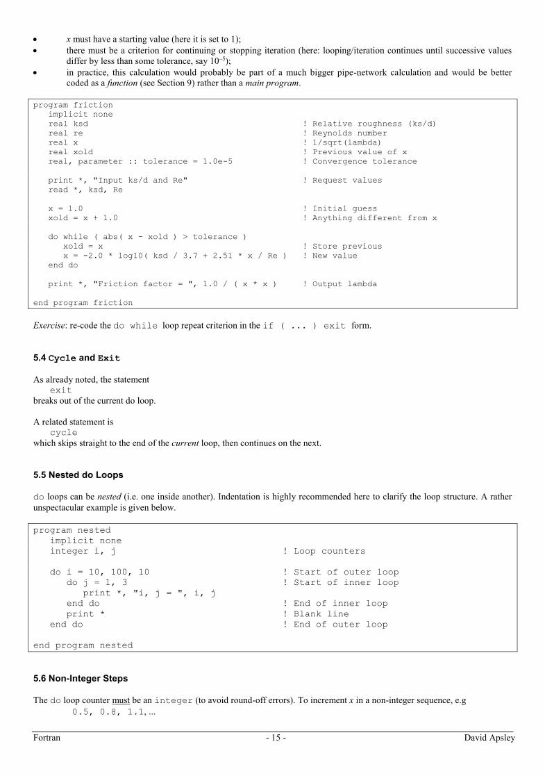
x must have a starting value (here it is set to 1);

there must be a criterion for continuing or stopping iteration (here: looping/iteration continues until successive values

differ by less than some tolerance, say 10–5);

in practice, this calculation would probably be part of a much bigger pipe-network calculation and would be better

coded as a function (see Section 9) rather than a main program.

program friction

implicit none

real ksd ! Relative roughness (ks/d)

real re ! Reynolds number

real x ! 1/sqrt(lambda)

real xold ! Previous value of x

real, parameter :: tolerance = 1.0e-5 ! Convergence tolerance

print *, "Input ks/d and Re" ! Request values

read *, ksd, Re

x = 1.0 ! Initial guess

xold = x + 1.0 ! Anything different from x

do while ( abs( x - xold ) > tolerance )

xold = x ! Store previous

x = -2.0 * log10( ksd / 3.7 + 2.51 * x / Re ) ! New value

end do

print *, "Friction factor = ", 1.0 / ( x * x ) ! Output lambda

end program friction

Exercise: re-code the do while loop repeat criterion in the if ( ... ) exit form.

5.4 Cycle and Exit

As already noted, the statement exit

breaks out of the current do loop.

A related statement is cycle

which skips straight to the end of the current loop, then continues on the next.

5.5 Nested do Loops

do loops can be nested (i.e. one inside another). Indentation is highly recommended here to clarify the loop structure. A rather

unspectacular example is given below.

program nested

implicit none

integer i, j ! Loop counters

do i = 10, 100, 10 ! Start of outer loop

do j = 1, 3 ! Start of inner loop

print *, "i, j = ", i, j

end do ! End of inner loop

print * ! Blank line

end do ! End of outer loop

end program nested

5.6 Non-Integer Steps

The do loop counter must be an integer (to avoid round-off errors). To increment x in a non-integer sequence, e.g

0.5, 0.8, 1.1, ...


you should work out successive values in terms of a separate integral counter by specifying:

an initial value (x0);

a step size (Δx)

the number of values to be output (Nx).

The successive values are:

x0, x0 +Δx, x0 +2Δx, … , x0 +(Nx-1)Δx.

The ith value is

x0 + (i – 1)Δx for i = 1, … , Nx.

program xloop

implicit none

real x ! Value to be output

real x0 ! Initial value of x

real dx ! Increment in x

integer nx ! Number of values

integer i ! Loop counter

print *, "Input x0, dx, nx" ! Request values

read *, x0, dx, nx

do i = 1, nx ! Start of repeated section

x = x0 + ( i - 1 ) * dx ! Value to be output

print *, x

end do ! End of repeated section

end program xloop

If one only uses the variable x once for each of its values (as above) one could simply combine the lines

x = x0 + ( i – 1 ) * dx

print *, x

as print *, x0 + ( i – 1 ) * dx

There is then no need for a separate variable x.

5.7 Implied Do Loops

This highly-compact syntax is often used to initialise arrays (see later) or for input/output of sequential data.

The general form is

( expression, index = start, end [, stride] )

and, like any other do-loop, it may be nested.

For example, the above lines do i = 1, nx

x = x0 + ( i - 1 ) * dx

print *, x

end do

can be condensed to the single line print *, ( x0 + ( i - 1 ) * dx, i = 1, nx )

(but note that, unless print * is replaced by a suitable formatted write - see later – then output will all be on one line).


6. DECISION-MAKING: if AND select

See Sample Programs B

Often a computer is called upon to perform one set of actions if some condition is met, and (optionally) some other set if it is not.

This branching or conditional action can be achieved by the use of IF or CASE constructs. A very simple use of if ...

else was given in the quadratic-equation program of Section 3.

6.1 The if Construct

There are several forms of if construct.

(i) Single statement.

if ( logical expression ) statement

(ii) Single block of statements.

if ( logical expression ) then

things to be done if true

end if

(iii) Alternative actions.

if ( logical expression ) then

things to be done if true

else

things to be done if false

end if

(iv) Several alternatives (there may be several else ifs, and there may or may not be an else).

if ( logical expression-1 ) then

.........

else if ( logical expression-2 ) then

.........

[else

.........

]

end if

As with do loops, if constructs can be nested. (Again, indentation is very helpful for identifying code structure).


6.2 The select Construct1

The select construct is a convenient (and sometimes more readable and/or efficient) alternative to an if ... else if

... else construct. It allows different actions to be performed depending on the set of outcomes (selector) of a particular

expression.

The general form is:

select case ( expression )

case ( selector-1 )

block-1

case ( selector-2 )

block-2

[case default

default block

]

end select

expression is an integer, character or logical expression. It is often just a simple variable.

selector-n is a set of values that expression might take.

block-n is the set of statements to be executed if expression lies in selector-n.

case default is used if expression does not lie in any other category. It is optional.

Selectors are lists of non-overlapping integer or character outcomes, separated by commas. Outcomes can be individual values

(e.g. 3, 4, 5, 6) or ranges (e.g. 3:6). These are illustrated below and in the week’s examples.

Example. What type of key have I pressed?

program keypress

implicit none

character letter

print *, "Press a key"

read *, letter

select case ( letter )

case ( 'A', 'E', 'I', 'O', 'U', 'a', 'e', 'i', 'o', 'u' )

print *, "Vowel"

case ( 'B':'D', 'F':'H', 'J':'N', 'P':'T', 'V':'Z', &

'b':'d', 'f':'h', 'j':'n', 'p':'t', 'v':'z' )

print *, "Consonant"

case ( '0':'9' )

print *, "Number"

case default

print *, "Something else"

end select

end program keypress

1 Similar to, but considerably more flexible than, the switch construct in C or C++.


7. ARRAYS

See Sample Programs C

In geometry it is common to denote coordinates by x1, x2, x3 or {xi}. The elements of matrices are written as a11, a12, ..., amn or

{aij}. These are examples of subscripted variables or arrays.

Mathematically, we often denote the whole array by its unsubscripted name; e.g. x for {xi} or a for {aij}. Whilst subscripted

variables are important in any programming language, it is the ability to refer to an array as a whole, without subscripts, which

makes Fortran particularly valuable in engineering. The ability to refer to just segments of it, e.g. the array section x(4:10) is

just the icing on the cake.

When referring to individual elements, subscripts are enclosed in parentheses; e.g. x(1), a(1,2), etc.2

7.1 One-Dimensional Arrays (Vectors)

Example. Consider the following program to fit a straight line to the set of points (x1,y1), (x2,y2), … , (xn,yn) and

then print them out, together with the best-fit straight line. The data file is assumed to be of the form shown

right and the best-fit straight line is cmxy where

𝑚 =

∑ 𝑥𝑦𝑛

− �̅��̅�

∑ 𝑥2

𝑛− �̅�2

, 𝑐 = �̅� − 𝑚�̅� where �̅� =∑ 𝑥

𝑛 , �̅� =

∑ 𝑦

𝑛

(Input/output using files will be covered more fully in Section 10. Just accept the read() and write() statements for now.)

program regression

implicit none

integer n ! Number of points

integer i ! A counter

real x(100), y(100) ! Arrays to hold the points

real sumx, sumy, sumxy, sumxx ! Various intermediate sums

real m, c ! Line slope and intercept

real xbar, ybar ! Mean x and y

sumx = 0.0; sumy = 0.0; sumxy = 0.0; sumxx = 0.0

! Initialise sums

open( 10, file = "pts.dat" ) ! Open the data file; attach to unit 10

read( 10, * ) n ! Read number of points

! Read the rest of the marks, one per line, and add to sums

do i = 1, n

read( 10, * ) x(i), y(i)

sumx = sumx + x(i)

sumy = sumy + y(i)

sumxy = sumxy + x(i) * y(i)

sumxx = sumxx + x(i) ** 2

end do

close( 10 ) ! Finished with the data file

! Calculate best-fit straight line

xbar = sumx / n

ybar = sumy / n

m = ( sumxy / n - xbar * ybar ) / ( sumxx / n - xbar ** 2 )

c = ybar - m * xbar

print *, "Slope = ", m

print *, "Intercept = ", c

print "( 3( 1x, a10 ) )", "x", "y", "mx+c"

do i = 1, n

print "( 3( 1x, es10.3 ) )", x(i), y(i), m * x(i) + c

end do

end program regression

2 Note that languages like C or C++ use (separate) square brackets for subscripts; e.g. x[1], a[1][2].

n

x1 y1

x2 y2

...

xn yn


Many basic features of arrays are illustrated by this example. We will then use modern Fortran to improve it.

7.2 Array Declaration

Like any other variables, arrays need to be declared at the start of a program unit and memory space assigned to them. However,

unlike scalar variables, array declarations require both a type (integer, real, complex, character, logical, or a

derived type) and a size or dimension (number of elements).

In this case the two one-dimensional (rank-1) arrays x and y can be declared as of real type with 100 elements by the type-

declaration statement real x(100), y(100)

or using the dimension attribute:

real, dimension(100) :: x, y

Actually, since “100” is a “magic number” that we might need to change consistently in many places if we wished to change

array size, then it is safer practice to declare array size as a single parameter, e.g.: integer, parameter :: MAXSIZE = 100

real x(MAXSIZE), y(MAXSIZE)

By default, the first element of an array has subscript 1. It is possible to make the array start from subscript 0 (or any other

positive or negative integer) by declaring the lower array bound as well. For example, to start at 0 instead of 1: real x(0:99)

Warning: in the C, C++ and Java programming languages the lowest subscript is 0 and you can’t change that!

7.3 Dynamic Arrays

An obvious problem arises. What if the number of points n is greater than the declared size of the array (here, 100)? Well,

different compilers will do different and unpredicatable things – most resulting in crashes.

One not-very-satisfactory solution is to check for adequate space, prompting the user to recompile if necessary with a larger

array size: read( 10, * ) n

if ( n > MAXSIZE ) then

print *, "Sorry, n > MAXSIZE. Please recompile with larger array"

stop

end if

It is probably better to keep out of the way of administrative staff if they encounter this error message!

A far better solution is to use dynamic memory allocation: that is, the array size is determined (and computer memory allocated)

at run-time, not in advance during compilation. To do this one must use allocatable arrays as follows.

(i) In the declaration statement, use the allocatable attribute; e.g.

real, allocatable :: x(:), y(:)

Note that the shape, but not size, is indicated at compile-time by a single colon (:).

(ii) Once the size of the arrays has been identified at run-time, allocate them the required amount of memory: read( 10, * ) n

allocate( x(n), y(n) )

(iii) When the arrays are no longer needed, recover memory by de-allocating them: deallocate( x, y )

(Additional comments about automatic allocation and deallocation are given later.)


7.4 Array Input/Output and Implied do Loops

In the example, the lines do i = 1, n

read( 10, * ) x(i), y(i)

...

end do

mean that at most one pair of points can be input per line. With an implied do loop: read( 10, * ) ( x(i), y(i), i = 1, n )

the program will simply read the first n data pairs (separated by spaces, commas or line breaks) that it encounters. As all the

points are read in one go, they no longer need to be on separate lines, but are taken in order of availability.

A similar statement can be used for output. However, note that write( 11, * ) ( x(i), y(i), i = 1, n )

will write successive pairs out on the same line, unless told to do otherwise by a formatted record; e.g. write( 11, "( 2( 1x, es10.3 )" ) ( x(i), y(i), i = 1, n )

If we are to read or write a single array to its full capacity, then even the implied do loop is unnecessary; e.g. read( 10, * ) x

will read enough values to populate x fully.

7.5 Elemental Operations

Sometimes we want to do the same thing to every element of an array. In the above example, for each mark we form the square

of that mark and add to a sum. The array expression x * x

is a new array with elements {xi2} The expression

sum( x * x )

therefore produces xi2. (See the sum function later.)

Using many of these array features a shorter version of the program is given below. Note that use of the intrinsic function sum

obviates the need for extra variables to hold intermediate sums and there is a one-line implied do loop for both input and output.

program regression

implicit none

integer n ! Number of points

integer i ! A counter

real, allocatable :: x(:), y(:) ! Arrays to hold the points

real m, c ! Line slope and intercept

real xbar, ybar ! Mean x and y

open( 10, file = "pts.dat" ) ! Open data file; attach to unit 10

read( 10, * ) n ! Read number of points

allocate( x(n), y(n) ) ! Allocate memory to x and y

read( 10, * ) ( x(i), y(i), i = 1, n ) ! Read the rest of the marks

close( 10 ) ! Finished with the data file

! Calculate best-fit straight line

xbar = sum( x ) / n ! Use intrinsic function sum()

ybar = sum( y ) / n

m = ( sum( x * y ) / n - xbar * ybar ) & ! Use array operations x * y and x * x

/ ( sum( x * x ) / n - xbar ** 2 )

c = ybar - m * xbar

print *, "Slope = ", m

print *, "Intercept = ", c

print "( 3( 1x, a10 ) )", "x", "y", "mx+c"

print "( 3( 1x, es10.3 ) )", ( x(i), y(i), m * x(i) + c, i = 1, n )

deallocate( x, y ) ! Recover memory space (unnecessary here)

end program regression

Note that here the value n is assumed to be given as the first line of the file. If this is not given then a reasonable approach is

simply to read the file twice: the first time to count data pairs, the second to read them into an array allocated to the required size.


7.6 Matrices and Higher-Dimension Arrays

An mn array of numbers of the form

mnm

n

aa

aa

1

111

is called a matrix (or rank-2 array). The typical element is denoted aij. It has two subscripts.

Fortran allows matrices (two-dimensional arrays) and, in fact, arrays of up to 7 dimensions. (However, entities of the form aijklmno

have never found much application in engineering!)

In Fortran the declaration and use of a real 33 matrix might look like

real A(3,3)

A(1,1) = 1.0; A(1,2) = 2.0; A(1,3) = 3.0

A(2,1) = 4.0

etc.

Other (better) methods of initialisation will be discussed below.

Matrix Multiplication

Suppose A, B and C are 33 matrices declared by

real, dimension(3,3) :: A, B, C

The statement C = A * B

does element-by-element multiplication; i.e. each element of C is the product of the corresponding elements in A and B.

To do “proper” matrix multiplication use the standard matmul function:

C = matmul( A, B )

Obviously matrix multiplication is not restricted to 33 matrices. However, for matrix multiplication to be legitimate, matrices

must be conformable; i.e. the number of columns of A must equal the number of rows of B.

A similarly useful function is that computing the transpose of a matrix: C = transpose( A )

7.7 Terminology

The rank of an array is the number of dimensions.

The extents of an array are the number of elements in each dimension.

The shape of an array is the collection of extents.

The size of an array is the total number of elements (i.e. the product of the extents).

7.8 Array Initialisation

One-dimensional arrays

The oldest forms of initialisation are:

separate statements; e.g, A(1) = 2.0; A(2) = 4.0; A(3) = 6.0; A(4) = 8.0; A(5) = 10.0

data statement:

data A / 2.0, 4.0, 6.0, 8.0, 10.0 /

loop and formula (if there is one): do i = 1, 5

A(i) = 2 * i

end do


reading from file

With modern Fortran we can do whole-array assignments or array operations:

whole-array assignment (see Section 7.10 below) to a constant: A = 2.0

or in terms of other arrays: A = B + C

array constructor: either(/ .... /)or the more modern form [ .... ]

A = (/ 2.0, 4.0, 6.0, 8.0, 10.0 /)

or A = [ 2.0, 4.0, 6.0, 8.0, 10.0 ]

Array constructors can be combined with a whole-array operation: A = 2 * [ 1.0, 2.0, 3.0, 4.0, 5.0 ]

or a combination of array constructor and implied do loop: A = [ ( 2 * i, i = 1, 5 ) ]

(With an up-to-date compiler) an allocatable array can be automatically allocated and assigned (or reallocated and

reassigned) without a separate allocate (or deallocate) statement. Thus:

real, allocatable :: A(:)

A = [ 2.0, 4.0, 6.0, 8.0, 10.0 ]

will allocate the array as size 5, with no need for allocate( A(5) )

in between. Moreover, if we subsequently write, for example, A = [ ( 2 * i, i = 1, 10 ]

then the array will be reallocated with a new size of 10.

If we simply want to add more elements to an allocatable array then we can write, e.g., A = [ A, 12.0, 14.0 ]

This quietly forms a temporary array constructor from array A plus the new elements, then reallocates and reassigns A.

In addition, locally allocated arrays (only existing within a single subroutine or function – see later) are automatically deallocated

at the end of that procedure, without a need for a deallocate statement.

Multi-Dimensional Arrays

Similar statements can also be used to initialise multi-dimensional arrays. However, the storage order of elements is important.

In Fortran, column-major storage is used; i.e. the first subscript varies fastest. For example, the storage order of a 33 matrix is A(1,1), A(2,1), A(3,1), A(1,2), A(2,2), A(3,2), A(1,3), A(2,3), A(3,3)

Warning: this storage order is the opposite convention to the C or C++ programming languages.

As an example, suppose we wish to create the array

1 2 34 5 67 8 9

with the usual matrix(row,column) indexing convention.

If we try

program main

implicit none

character(len=*), parameter :: fmt = "( 3( i2, 1x ) )"

integer row, col

integer A(3,3)

data A / 1, 2, 3, 4, 5, 6, 7, 8, 9 /

do row = 1, 3

write( *, fmt ) ( A(row,col), col = 1, 3 )

end do

end program main


then we obtain, rather disconcertingly, 1 4 7

2 5 8

3 6 9

We can compensate for the column-major order either by adjusting the order in the data statement: data A / 1, 4, 7, 2, 5, 8, 3, 6, 9 /

which is error-prone rather hard work. Alternatively, we could retain the original data statement but simply transpose A as our

first executable statement: data A / 1, 2, 3, 4, 5, 6, 7, 8, 9 /

A = transpose( A )

In modern usage one can use an array constructor instead of a data statement. Since, however, an array constructor is 1-

dimensional it must be combined with a call to the reshape function to put it in the correct shape (here, 33):

A = reshape( [ 1, 2, 3, 4, 5, 6, 7, 8, 9 ], [ 3, 3 ] )

A = transpose( A )

The first argument to the reshape function is the 1-d array, the second is the shape (set of extents) of the intended output.

These approaches all lead to the desired output 1 2 3

4 5 6

7 8 9

7.9 Array Expressions

Arrays are used where large numbers of data elements are to be treated in similar fashion. Fortran allows a very powerful

syntactic shorthand to be used whereby, if the array name is used in a numeric expression without subscripts, then the operation

is assumed to be performed on every element of an array. This is far more concise than older versions of Fortran, where it was

necessary to use do loops, and, indeed many other computer languages.

For example, suppose that arrays x, y and z are declared with, say, 10 elements:

real, dimension(10) :: x, y, z

Assignment

x = 5.0

sets every element of x to the value 5.0.

Array Expressions

y = -3 * x

Sets yi to –3xi for each element of the respective arrays.

y = x + 3

Although 3 is only a scalar, yi is set to xi + 3 for each element of the arrays.

z = x * y

Sets zi to xiyi for each element of the respective arrays. Remember: this is “element-by-element” multiplication.

Array Arguments to Intrinsic Functions

y = sin( x )

Sets yi to sin(xi) for each element of the respective arrays. sin is said to be an elemental function, as are most of Fortran’s

intrinsic functions. In the Advanced course we shall see how to make our own functions do this.

7.10 Array Sections

An array section is a subset of an array and is denoted by a range operator

lower : upper : stride


for one particular dimension of the array. One or more of these may be omitted If lower is omitted it defaults to the lower bound

of that dimension; if upper is omitted then it defaults to the upper bound. If stride is omitted then it defaults to 1.

For example, if A is a rank-1 array with dimension 9 and elements 10, 20, 30, 40, 50, 60, 70, 80, 90 then

A(3:5) is [ 30, 40, 50 ]

A(:4) is [ 10, 20, 30, 40 ]

A(2::2) is [ 20, 40, 60, 80 ]

Note that array sections are themselves arrays and can be used in whole-array and elemental operations.

An important use is in reduction of rank for higher-rank arrays. For example, if A, B and C are rank-2 arrays (matrices) then

A(i,:) is the ith row of A

B(:,j) is the jth row of B

Thus, C(i,j) = sum( A(i,:) * B(:,j) )

forms the scalar product of the ith row of A and jth row of B, giving the(i,j) component of the matrix C = AB.

7.11 The where Construct

where is like an if construct applied to every element of an array. For example, to turn every non-zero element of an array a

into its reciprocal, one could write where ( A /= 0.0 )

A = 1.0 / A

end where

The element ( A /= 0.0 ) actually yields a mask, or logical array of the same shape as A, but whose elements are simply

true or false. A similar logical mask is used in the array functions ALL and ANY in the next subsection.

Note that the individual elements of a are never mentioned. {where, else, else where, end where} can be used

whenever one wants to use a corresponding {if, else, else if, end if} for each element of an array.

7.12 Array-handling Functions

Fortran’s use of arrays is extremely powerful, and many intrinsic routines are built into the language to facilitate array handling.

For example, a do-loop summation can be replaced by a single statement; e.g. sumx = sum( x )

This uses the intrinsic function sum, which adds together all elements of its array argument.

Most mathematical intrinsic routines are actually elemental, which means that they can be applied equally to scalar variables and

arrays.

For a full set of array-related functions please consult the recommended textbooks. However, subset that you may find useful are

given below.

A number of intrinsic routines exist to query the shape of arrays. Assume A is an array with 1 or more dimensions. Its rank is the

number of dimensions; its extents are the number of elements in each dimension; its shape is the collection of extents.

lbound( A ) returns a rank-1 array holding the lower bound in each dimension.

lbound( A, i ) returns an integer holding the lower bound in the ith dimension.

shape( A ) returns a rank-1 array giving the extents in each direction

size( A ) returns an integer holding the complete size of the array (product of its extents)

size( A, i ) returns an integer holding the extent in the ith dimension.

ubound( A ) returns a rank-1 array holding the upper bound in each dimension.

ubound( A, i ) returns an integer holding the upper bound in the ith dimension.

Algebra of vectors (rank-1 arrays)

dot_product( U, V ) returns the scalar product of U and V

Algebra of matrices (rank-2 arrays):

matmul( A, B ) returns the matrix multiple (rather than elemental multiple) of arrays A and B

transpose( A ) returns the transpose of matrix A


Reshaping arrays:

reshape( A, S ) A is a source array, S is the 1-d array of extents to which to reshape it

Scalar results:

sum( A ) returns the sum of all elements of A

product( A ) returns the product of all elements of A

minval( A ) returns the minimum value in A

maxval( A ) returns the maximum value in A

count( logical expr ) returns the number of elements of A fulfilling the logical condition

all ( logical expr ) returns .true. or .false. according as all elements of A fulfil the condition or not

any( logical expr ) returns .true. or .false. according as any elements of A fulfil the condition or not

An example of some of these for a rank-1 array is given below.

program test

implicit none

integer :: A(10) = [ 2, 3, 3, 6, 2, 8, 5, 5, 1, 12 ]

integer :: value = 5

print *, "A: ", A

print *, "Size of A: ", size( A )

print *, "Lower bound of A is ", lbound( A )

print *, "Upper bound of A is ", ubound( A )

print *, "Sum of the elements of A is ", sum( A )

print *, "Product of the elements of A is ", product( A )

print *, "Maximum value in A is ", maxval( A )

print *, "Minimum value in A is ", minval( A )

print *, count( A == value ), " values of A are equal to ", value

print *, "Any value of A > 10? ", any( A > 10 )

print *, "All value of A > 10? ", all( A > 10 )

end program test

A: 2 3 3 6 2 8 5 5 1 12

Size of A: 10

Lower bound of A is 1

Upper bound of A is 10

Sum of the elements of A is 47

Product of the elements of A is 518400

Maximum value in A is 12

Minimum value in A is 1

2 values of A are equal to 5

Any value of A > 10? T

All value of A > 10? F


8. TEXT HANDLING


Fortran (FORmula TRANslation) was originally developed for scientific and engineering calculations, not word-processing.

However, modern versions now have extensive text-handling capabilities.

8.1 Character Constants and Variables

A character constant (or string) is a series of characters enclosed in delimiters, which may be either single (') or double (")

quotes; e.g.

'This is a string' or "This is a string"

The delimiters themselves are not part of the string.

Delimiters of the opposite type can be used within a string with impunity; e.g. print *, "This isn't a problem"

However, if the bounding delimiter is to be included in the string then it must be doubled up; e.g. print *, 'This isn''t a problem.'

Character variables must have their length – i.e. number of characters – declared in order to set aside memory. The following

will declare a character variable word of length 10:

character(len=10) word

To save counting characters, an assumed length (indicated by len=* or, simply, *) may be used for character variables with the

parameter attribute; i.e. those whose value is fixed. e.g.

character(len=*), parameter :: UNIVERSITY = "Manchester"

If len is not specified for a character variable then it defaults to 1; e.g.

character letter

Character arrays are simply subscripted character variables. Their declaration requires a dimension statement in addition to

length; e.g. character(len=3), dimension(12) :: months

or, equivalently, character(len=3) months(12)

This array might then be initialised by, for example, data months / "Jan", "Feb", "Mar", "Apr", "May", "Jun", &

"Jul", "Aug", "Sep", "Oct", "Nov", "Dec" /

or declared and initialised together: character(len=3) :: months(12) = [ "Jan", "Feb", "Mar", "Apr", "May", "Jun",&

"Jul", "Aug", "Sep", "Oct", "Nov", "Dec" ]

8.2 Character Assignment

When character variables are assigned they are filled from the left and padded with blanks if necessary. For example, if

university is a character variable of length 7 then

university = "UMIST" fills university with "UMIST "

university = "Manchester" fills university with "Manches"

8.3 Character Operators

The only character operator is // (concatenation) which simply sticks two strings together; e.g.

"Man" // "chester" "Manchester"


8.4 Character Substrings

Character substrings may be extended in a similar fashion to sub-arrays; (in a sense, a character string is an array of single

characters). e.g. if city is "Manchester" then

city(2:5) is "anch"

city (:3) is "Man"

city (7:) is "ster"

city(5:5) is "h"

city( : ) is "Manchester"

Note: if we want the ith letter then we cannot write city(i) as for arrays, but instead city(i:i).

8.5 Comparing and Ordering

Each computer system has a character-collating sequence that specifies the intrinsic ordering of the character set. The most

common is ASCII (shown below). ‘Less than’ (<) and ‘greater than’ (>) strictly refer to the position of the characters in this

collating sequence.

0 1 2 3 4 5 6 7 8 9

30 space ! " # $ % & '

40 ( ) * + , - . / 0 1

50 2 3 4 5 6 7 8 9 : ;

60 < = > ? @ A B C D E

70 F G H I J K L M N O

80 P Q R S T U V W X Y

90 Z [ \ ] ^ _ ` a b c

100 d e f g h i j k l m

110 n o p q r s t u v w

120 x y z { | } ~ del

The ASCII character set. Characters 0-31 are control characters like [TAB] or [ESC] and are not shown.

The Fortran standard requires that upper-case letters A-Z and lower-case letters a-z are separately in alphabetical order, that the

numerals 0-9 are in numerical order, and that a blank space comes before both. It does not, however, specify whether numbers

come before or after letters in the collating sequence, or lower case comes before or after upper case. Provided there is consistent

case, strings can be compared on the basis of dictionary order. However, the standard gives no guidance when comparing letters

with numerals or upper with lower case using < and >. Instead, we can use the llt (logically-less-than) and lgt (logically-

greater-than) functions, which ensure comparisons according to the ASCII ordering. Similarly there are lle (logically-less-than-

or-equal) and lge (logically-greater-than-or-equal) functions.

Examples. The following logical expressions are all “true” (which may cause some controversy!): "Manchester City" < "Manchester United"

"Mickey Mouse" > "Donald Trump"

"First year" < "Second year"

Examples.

100 < 20 gives .false. as a numeric comparison

"100" < "20" gives .true. as a string comparison (comparison based on the first character)

and

LLT( "1st", "First" ) gives .true. by ASCII ordering according to first character.


8.6 Intrinsic Subprograms With Character Arguments

The more common character-handling routines are given in Appendix A4. A full set is given in the recommended textbooks.

Position in the Collating Sequence

char( i ) character in position i of the system collating sequence;

ichar( c ) position of character c in the system collating sequence.

The system may or may not use ASCII as a collating system, but the following routines are always available:

achar( i ) character in position i of the ASCII collating sequence;

iachar( c ) position of character c in the ASCII collating sequence.

The collating sequence may be used, for example, to sort names into alphabetical order or convert between upper and lower case,

as in the following example.

Example. Since the separation of ‘b’ and ‘B’, ‘c’ and ‘C’ etc. in the collating sequence is the same as that between ‘a’ and ‘A’,

the following subroutine may be used successively for each character to convert lower to upper case. If letter has lower case

it will:

convert to its number using ichar( )

add the numerical difference between upper and lower case: ichar('A')-ichar('a')

convert back to a character using char( )

subroutine uc( letter )

implicit none

character (len=1) letter

if ( letter >= 'a' .and. letter <= 'z' ) then

letter = char( ichar( letter ) + ichar( 'A' ) - ichar( 'a' ) )

end if

end subroutine uc

Length of String

len( string ) declared length of string, even if it contains trailing blanks;

trim( string ) same as string but without any trailing blanks;

len_trim( string ) length of string with any trailing blanks removed.

Justification

adjustl( string ) left-justified string

adjustr( string ) right-justified string

Finding Text Within Strings

index( string, substring ) position of first (i.e. leftmost) occurrence of substring in string

scan( string, set ) position of first occurrence of any character from set in string

verify( string, set ) position of first character in string that is not in set

Each of these functions returns 0 if no such position is found.

To search for the last (i.e. rightmost) rather than first occurrence, add a third argument .true., e.g.:

index( string, substring, .true. )

Other

repeat( string, ncopies ) produces a character made up of ncopies concatenations of string.

e.g. character(len=*), parameter :: base = repeat( "ABC", 4 )

produces base = "ABCABCABCABC"


9. FUNCTIONS AND SUBROUTINES


All major computing languages allow complex and/or repetitive programs to be broken down into simpler procedures or

subprograms, each carrying out particular well-defined tasks, often with different values of their arguments. In Fortran these

procedures are called subroutines and functions. Examples of the action carried out by a single procedure might be:

calculate the distance 22 yxr of a point (x,y) from the origin;

calculate 1.2)...1(! nnn for a positive integer n

As these are likely to be needed several times, it is appropriate to code them as a distinct procedure.

9.1 Intrinsic Procedures

Certain intrinsic procedures are defined by the Fortran standard and must be provided by an implementation’s libraries. For

example, the statement y = x * sqrt( x )

invokes an intrinsic function sqrt, with argument x, and returns a value (in this case, the square root of its argument) which is

then employed to evaluate the numeric expression.

Useful mathematical intrinsic procedures are listed in Appendix A4. The complete set required by the standard is given in the

recommended textbooks. Particular Fortran implementations may also supply additional procedures, but you would then be tied

to that particular compiler.

9.2 Program Units

There are four types of program unit:

main programs

subroutines

functions

modules

Each source file may contain one or more program units and is compiled separately. (This is why one requires a link stage after

compilation.) The advantage of separating program units between source files is that other programs can make use of a particular

subset of the routines.

Main Programs

Every Fortran program must contain exactly one main program which should start with a program statement. This may invoke

functions or subroutines which may, in turn, invoke other procedures.

Subroutines

A subroutine is invoked by

call subroutine-name ( argument list )

The subroutine carries out some action according to the value of the arguments. It may or may not change the values of these

arguments. There may be no arguments (in which case the brackets are optional).

Functions

A function is invoked simply by using its name (and argument list) in a numeric expression; e.g. a function radius:

distance = radius( x, y )

Within the function’s source code its name (without arguments) is treated as a variable and should be assigned a value, which is

the value of the function on exit – see the example below3. A function should be used when a single variable is to be returned. It

is permissible, but not usual practice, for a function to change its arguments – a better vehicle in that case would be a subroutine.

3 An alternative version, using the name in a result clause, is given in the Advanced part of the course.


Functions and subroutines are collectively called procedures. A subroutine is like a void function, and a function like a type-

returning function in C or C++.

Modules (see Section 11)

Functions and subroutines may be internal (i.e. contain-ed within and only accessible to one particular program unit) or

external (and accessible to all). Related internal routines are better gathered together in special program units called modules.

Their contents are then made available collectively to other program units by the initial statement

use module-name

Modules have many other uses and are increasingly “the way that Fortran is evolving”; we will examine some of them in later

sections.

The basic forms of main program, subroutines and functions with no internal subprograms are very similar and are given below.

As usual, [ ] denotes something optional but, in these cases, it is strongly recommended.

The first statement defines the type of program unit, its name and its arguments. function procedures must also have a return

type. This must be declared either in the initial statement (as here) or in a separate type declaration within the routine itself.

Procedures pass control back to the calling program when they reach the end statement. Sometimes it is required to pass control

back before this. This is effected by the return statement. An early death to the program as a whole can be achieved by a

stop statement.

Many actions could be coded as either a function or a subroutine. For example, consider a program which calculates distance

from the origin, 2/122 )( yxr :

In the first example, the calling program must declare the type of the function (here, real) amongst its other type declarations.

It is optional, but good practice, to identify external procedures by using either an external attribute in the type statement

(first example) or a separate external statement (second example). This makes clear what external routines are being used and

Main program

[program [name]]

use statements [implicit none]

type declarations

executable statements

end [program [name]]

Subroutines

subroutine name (argument-list)


type declarations


end [subroutine [name]]

Functions

[type] function name (argument-list)


type declarations


end [function [name]]

(Using a function)

program example

implicit none

real x, y

real, external :: radius

print *, "Input x, y"

read *, x, y

print *, "Distance = ", radius( x, y )

end program example

!===============================

real function radius( a, b )

implicit none

real a, b

radius = sqrt( a ** 2 + b ** 2 )

end function radius

(Using a subroutine)

program example

implicit none

real x, y

real radius

external distance

print *, "Input x, y"

read *, x, y

call distance( x, y, radius )

print *, "Distance = ", radius

end program example

!===============================

subroutine distance( a, b, r )

implicit none

real a, b, r

r = sqrt( a ** 2 + b ** 2 )

end subroutine distance


ensures that if the Fortran implementation supplied an intrinsic routine of the same name then the external routine would

override it. (Function names can themselves be passed as arguments; in that case the external is obligatory for a user

procedure unless an explicit interface is supplied – see the Advanced course).

Note that all variables in the functions or subroutines above have scope the program unit in which they are declared; that is, they

have no connection with any variables of the same name in any other program unit.

9.3 Subprogram Arguments

The arguments in the function or subroutine statement are called dummy arguments: they exist only for the purpose of

defining that procedure and have no connection to other variables of the same name in other program units. The arguments used

when the procedure is actually invoked are called the actual arguments. They may be variables (e.g. x, y), constants (e.g. 1.0,

2.0) or expressions (e.g. 3.0 + x, or 2.0 / y), but they must be of the same type and number as the dummy arguments.

For example, the radius function above could not be invoked as radius( x ) (too few arguments) or as

radius( 1, 2 ) (arguments of the wrong type: integer rather than real). Even if they are variables there is no reason why

actual arguments have to have the same name as the dummy arguments (though that is quite common). On occasion there may be

no arguments.

You may wonder how it is, then, that many intrinsic subprograms can be invoked with different types of argument. For example,

in the statement y = exp( x )

x may be real or complex, scalar or array. This is achieved by a process known as overloading and exp is called a generic,

elemental function. These properties are dealt with in the Advanced course.

Passing by Name/Passing by Reference

In Fortran, if the actual arguments are variables, they are passed by reference, and their values will change if the values of the

dummy arguments change in the subprogram. If, however, the actual arguments are either constants or expressions, then the

arguments are passed by value; i.e. the values are copied into the subprogram’s dummy arguments.

Warning: in C, all arguments are, by default, passed by value – a feature that necessitates the use of pointers to change values.

C++ has extended this to include “implied pointers” or “references”.

Declaration of Intent

Because input variables passed as arguments may be changed unwittingly if the dummy arguments change within a subprogram,

or, conversely, because a particular argument is intended as output and so must be assigned to a variable (not a constant or

expression), it is good practice to declare whether dummy arguments are intended as input or output by using the intent

attribute. e.g. in the above example: subroutine distance( a, b, r )

real, intent(in) :: a, b

real, intent(out) :: r

This signifies that dummy arguments a and b must not be changed within the subroutine and that the third actual argument must

be a variable. There is also an intent(inout) attribute.

9.4 The save Attribute

By default, variables declared within a subprogram do not retain their values between successive calls to the same subprogram.

This behaviour can be overridden by the save attribute; e.g. real, save :: x

which will store the value of x for the next time the routine is used. Variables initialised by data statements are automatically

saved, as are variables in modules.

save with a list of variables can also be used as a separate statement to save those variables:

real x, y, z

save x, y

If save is used without any list then all variables in that program unit are saved.


9.5 Array Arguments

Arrays can be passed as arguments in much the same way as scalars, except that the procedure must know the dimensions of the

array. In this section we assume that they are passed as explicit-shape arrays; that is, array dimensions are known at compile

time. (The Advanced course will look at other ways of specifying array size for a procedure argument.)

Fixed array size – usually for smaller arrays such as coordinate vectors; e.g. subroutine geometry( x )

real x(3)

Pass the array size as an argument; e.g. subroutine geometry( ndim, x )

real x(ndim)

9.6 Character Arguments

Dummy arguments of character type behave in a similar manner to arrays – their length must be made known to the subprogram.

However, a character dummy argument may always be declared with assumed length (determined by the length of the actual

argument); e.g. call example( "David" )

... subroutine example( person )

character(len=*) person ! Determines the length from the actual argument


10. INPUT/OUTPUT

See Sample Programs D

Hitherto we have used simple list-directed input/output (i/o) with the standard input/output devices (keyboard and screen):

read *, list

print *, list

This section describes how to:

use formatted output to control the layout of results;

read from and write to files;

use additional specifiers to provide advanced i/o control.

10.1 READ and WRITE

General list-directed i/o is performed by the statements

read( unit, format ) list

write( unit, format ) list

unit can be one of:

an asterisk *, meaning the standard i/o device (usually the keyboard/screen);

a unit number in the range 1 to 99 which has been associated with an external file (see below);

a character variable (internal file): this is the simplest way of interconverting numbers and strings.

format can be one of:

an asterisk *, meaning list-directed i/o;

a label associated with a format statement containing a format specification;

a character constant or expression evaluating to a format specification.

list is a set of variables or expressions to be input or output.

In terms of the simpler i/o statements used before:

read( *, * ) is equivalent to read *

write( *, * ) is equivalent to print *

10.2 Input/Output With Files

Before an external file can be read from or written to, it must be associated with a unit number by an open statement. e.g. to

associate the external file input.dat (in the current working directory) with the unit number 10:

open( 10, file="input.dat" )

One can then read from the file using

read( 10, ... ) ...

or write to the file using

write( 10, ... ) ...

Although units are automatically disconnected at program end it is good practice (and it frees the unit number for re-use) if it is

explicitly closed when no longer needed. For the above example, this means: close( 10 )

In general the unit number (10 in the above example) may be any number in the range 1-99. Historically, however, 5 and 6 have

been preconnected to the standard input and standard output devices, respectively.

The example above shows open used to attach a file for sequential (i.e. beginning-to-end), formatted (i.e. human-readable)

access. This is the default and is all we shall have time to cover in this course. However, Fortran can be far more flexible – see

for example the recommended textbooks.


10.3 Formatted WRITE

In the output statement

write( unit, format ) list

list is a comma-separated set of constants or variables to be output, unit indicates where the output is to go, whilst format

indicates the way in which the output is to be set out. If format is an asterisk * then the computer will choose how to set it out.

However, if you wish to display output in a particular way, for example in neat columns, then you must specify the format more

carefully.

Alternative Formatting Methods

The following code fragments are equivalent means of specifying the same output format. They show how i, f and e edit

specifiers display the number 55 in integer, fixed-point and floating-point formats.

(i) Using a format statement with a label (here 150):

write( *, 150 ) 55, 55.0, 55.0

... 150 format( 1x, i3, 1x, f5.2, 1x, e8.2 )

The format statement can be put anywhere within the executable statements of that program unit.

(ii) Putting the format directly into the write statement:

write( *, "( 1x, i3, 1x, f5.2, 1x, e8.2 )" ) 55, 55.0, 55.0

(iii) Putting the format in a character variable C (either in its declaration as here, or a subsequent assignment):

character(len=*), parameter :: fmt = "( 1x, i3, 1x, f5.2, 1x, e8.2 )"

... write( *, fmt ) 55, 55.0, 55.0

Any of these will output (to the screen): 55 55.00 0.55e+02

Terminology

A record is an individual line of input/output.

A format specification describes how data is laid out in (one or more) records.

A label is a number in the range 1-99999 preceding a statement on the same line. The commonest uses are in conjunction with

format statements and to indicate where control should pass following an i/o error.

Edit Descriptors

A format specification consists of a series of edit descriptors (e.g. i4, f7.3) separated by commas and enclosed by brackets.

The commonest edit descriptors are:

iw integer in a field of width w; note that i0 in output means “whatever length is necessary”;

fw.d real, fixed-point format, in a field of width w with d decimal places;

ew.d real, floating-point (exponential) format in a field of width w with d decimal places;

gw.d real format in whichever of fw.d or gw.d is more appropriate to the output;

npew.d floating point format as above with n significant figures in front of the decimal point;

esw.d “scientific” notation; i.e. 1 significant figure in front of the decimal point;

enw.d “engineering” notation; i.e. multiples of 3 significant figures in front of the decimal point;

lw logical value (T or F) in a field of width w;

aw character string in a field of width w;

a character string of length determined by the output list; for input: a whole line of data;

"text" a character string actually placed in the format specification;

nx n spaces

tn move to position n of the current record;

/ start a new record;

* repeat the following bracketed subformat as often as needed;

: finish the record here if there is no further data to be read/written.


This is only a fraction of the available edit descriptors – see the recommended textbooks.

Notes:

(1) If the required number of characters is less than the specified width then the output will be right-justified in its field.

(2) (For numerical output) if the required number of characters exceeds the specified width then the field will be filled with

asterisks. E.g, attempting to write 999 with edit descriptor i2 will result in **.

(3) Attempting to write output using an edit specifier of the wrong type (e.g. 3.14 in integer specifier i4) will result in a

run-time – but not compile-time error; try it so that you can recognise the error message.

(4) The format specifier will be used repeatedly until the output list is exhausted. Each use will start a new record. For

example, write( *, "( 1x, i2, 1x, i2, 1x, i2 )" ) ( i, i = 1, 5 )

will produce the following lines of output: 1 2 3

4 5

(5) If the whole format specifier isn’t required (as in the last line above) the rest is simply ignored.

Repeat Counts

Format specifications can be simplified by collecting repeated sequences together in brackets with a repeat factor. For example,

the code example above could also be written write( *, "( 3( 1x, i2 ) )" ) ( i, i = 1, 5 )

Because the format string allows 3 integers per record, the line breaks after records result in two lines of output: 1 2 3

4 5

However, the repeat count can also be *, which means “as often as necessary”: write( *, "( *( 1x, i2 ) )" ) ( i, i = 1, 5 )

This produces 1 2 3 4 5

Colon Editing

CSV (comma-separated values) files – with data fields separated by commas – are widely used for tabular data, and can be easily

read or written by Microsoft Excel. If we try to output a comma after every item, by, e.g., write( *, "( *( i2, ’,’ ) )" ) ( i, i = 1, 5 )

then we obtain 1, 2, 3, 4, 5,

with a trailing comma. The fix for this is to precede what we don’t want (just a comma in this instance) by :, which means “stop

here if there is no more data”. So write( *, "( *( i2, :, ’,’ ) )" ) ( i, i = 1, 5 )

produces 1, 2, 3, 4, 5

without the trailing comma.

Historical Baggage: Carriage Control

It is recommended that the first character of an output record be a blank. This is best achieved by making the first edit specifier

either 1x (one blank space) or t2 (start at the second character of the record). In the earliest versions of Fortran the first

character effected line control on a line printer. A blank meant ‘start a new record’. Although such carriage control is long gone,

a few i/o devices may still ignore the first character of a record.


10.4 The read Statement

In the input statement

read( unit, format ) list

list is a set of variables to receive the data. unit and format are as for the corresponding write statement.

Although formatted reads are possible (an example is given in the example programs D), it is uncommon for format to be

anything other than * (i.e. list-directed input). If there is more than one variable in list then the input items can be separated by

blank spaces, commas or simply new lines.

Notes.

(1) Each read statement will keep reading values from the input until the variables in list are assigned to, even if this

means going on to the next record.

(2) Each read statement will, by default, start reading from a new line, even if there is input data unread on the previous

line. In particular, the statement read( *, * )

(with no list) will simply skip a line of unwanted data.

(3) The variables in list must correspond in type to the input data – there will be a run-time error if you try to read a number

with a decimal point into an integer variable, or some text into a real variable, for example.

Example. The following program reads the first two items from each line of an input file input.dat and writes their sum to a

file output.dat.

program io

implicit none

integer i

integer a, b

open( 10, file="input.dat" )

open( 20, file="output.dat" )

do i = 1, 4

read( 10, * ) a, b

write( 20, * ) a + b

end do

close( 10 )

close( 20 )

end program io

A sample input file (input.dat) is:

10 3

-2 33

3 -6

40 15

Exercise:

(1) Type the source code into file io.f90 (say) and the input data into input.dat (saving it in the same folder).

Compile and run the program and check the output file.

(2) Modify the program to write the output to screen instead of to file.

(3) Modify the program to format the output in a tidy column.

(4) Try changing the input file and predicting/observing what happens. Note any run-time error messages.

(i) Change the first data item from 10 to 10.0 – why does this fail at run-time?

(ii) Add an extra number to the end of the first line – does this make any difference to output?

(iii) Split the last line with a line break – does this make any difference to output?

(iv) Change the loop to run 3 times (without changing the input data).

(v) Change the loop to run 5 times (without changing the input data).


10.5 Repositioning Input Files

rewind unit repositions the file attached to unit at the first record.

backspace unit repositions the file attached to unit at the start of the previous record.

Obviously, neither will work if unit is attached to the keyboard!

10.6 Additional Specifiers

The general form of the read statement is

read ( unit, format[, specifiers] )

Some useful specifiers are:

iostat = integer-variable assigns integer-variable with a number indicating status

err = label jump to label on an error (e.g. missing data or data of the wrong type);

end = label jump to label when the end-of-file marker is reached.

iostat returns zero if the read is successful, implementation-dependent negative integers for end-of-file (EOF) or end-of-

record (EOR), and positive integers for other errors.

Non-Advancing Input/Output

By default, each read or write statement automatically concludes with a carriage return/line feed. This can be prevented with

an advance="no" specifier; e.g. write( *, "( a )", advance="NO" ) "Enter a number: "

read( *, * ) i

Note that a format specifier (here, just "( a )" for any number of characters) must be used for non-advancing i/o, even for a

simple output string. The following statement won’t work: write( *, *, advance="no" ) "Enter a number: "

Assuming ch has been declared as a character of length 1 then one character at a time can be read from a text file attached to

unit 10 by: read( 10, "( a1 )", iostat=io, advance="no" ) ch By testing the state of variable io after the end of each read (it will be 0 if the read is successful, non-zero otherwise), we can

determine when we have reached the end of file.

10.7 Internal Files – Characters

Input and output can be redirected to character variables rather than input files. (The usage is very close to the use of a

stringstream in C++.) This can be very useful for a number of applications, including:

assembling format strings when their form isn’t known until run-time;

creating text snippets to use in graphical output;

hard-coding input and output for testing or demonstration, to avoid the need for input files (e.g. for online compilers).

program example

implicit none

integer i, n

character(len=100) input

real, allocatable :: x(:)

input = "5 2.3 1.8 0.9 0.1 -2.4" ! Input data

read( input, * ) n ! Number of points

allocate( x(n) )

read( input, * ) n, ( x(i), i = 1, n ) ! Reread number, then all data

write( *, "( a, *( 1x, f6.2 ) )" ) "Data is ", x

end program example

Data is 2.30 1.80 0.90 0.10 -2.40


11. MODULES

See Sample Programs D

Modules are the fourth type of program unit (after main programs, subroutines and functions). They were new in Fortran 90 and

typify modern programming practice. Modules will be used much more in the Advanced course.

A module has the form:

module module-name

type declarations [contains

internal subprograms]

end module [module-name]

The main uses of a module are:

to allow sharing of variables between multiple program units;

to collect together related internal subprograms (functions or subroutines);

to provide explicit interfaces to user-defined types, advanced procedures etc.;

to define a class in object-oriented programming.

Other program units have access to these module variables and internal subprograms via the statement

use modulename

which should be placed at the start of the program unit (before any implicit none or type statements).

Modules make redundant older elements of Fortran such as common blocks (used to share variables), statement functions (one-

line internal functions) and the (never-actually-standardised) include statement.

By having a single place to collect shared variables, they avoid long argument lists and the need to modify code in many separate

places if the variables to be shared change. Thus, they make it much easier to upgrade or modify complex code.

11.1 Sharing Variables

Variables are passed between one program unit and another via argument lists. For example a program may call a subroutine

polars by

call subroutine polars( x, y, r, theta )

The program passes x and y to the subroutine and receives r and theta in return. Any other variables declared in one program

unit are completely unknown to the other, even if they have the same name. Other routines may also call polars in the same

way.

Communication by argument list alone is OK provided the argument list is (a) short; and (b) unlikely to change with code

development. Problems arise if:

a large number of variables need to be shared between program units; (the argument list becomes long and unwieldy);

code is under active development; (the variables being shared may need to be changed, and will have to be changed

consistently in every program unit making that subroutine call).

Modules solve these problems by maintaining a central collection of variables which can be modified when required. Any

changes need only be made in the module. A use statement makes this available to each subprogram that needs it.

11.2 Internal Functions

Subroutines and functions can be external or can be internal to bigger program units. Internal subprograms are accessible only to

the program unit in which they are defined (which is a bit selfish!) and are only of use for short, simple functions specific to that

program unit. The best vehicle for an internal function is a module, because its internal functions or subroutines are accessible to

all the subprograms that use that module.

The following (somewhat trite) example illustrates how program cone uses a routine from module geom to find the volume of a

cone. Note the use statement in the main program and the structure of the module. The arrangement is convenient because if we

later decide to add a new global variable or geometry-related function (say, a function volume_cylinder) it is easy to do so

within the module.


module Geom

! Functions to compute areas and volumes

implicit none

! Shared variables

real, parameter :: PI = 3.14159

contains

! Internal subprograms

real function area_circle( r )

real r

area_circle = PI * r ** 2

end function area_circle

real function area_triangle( b, h )

real b, h

area_triangle = 0.5 * b * h

end function area_triangle

real function area_rectangle( w, l )

real w, l

area_rectangle = w * l

end function area_rectangle

real function volume_sphere( r )

real r

volume_sphere = ( 4.0 / 3.0 ) * PI * r ** 3

end function volume_sphere

real function volume_cuboid( w, l, h )

real w, l, h

volume_cuboid = w * l * h

end function volume_cuboid

real function volume_cone( r, h )

real r, h

volume_cone = PI * r ** 2 * h / 3.0

end function volume_cone

end module Geom

program cone

use Geom ! Declare use of module

implicit none

real radius, height

print *, "Input radius and height"

read *, radius, height

print *, "Volume: ", volume_cone( radius, height )

end program cone

Note that the internal functions of the module (as well as any program units using the module) automatically have access to any

module variables above the contains statement (here, just PI).

11.3 Compiling Programs With Modules

The module may be in the same source file as other program units or it may be in a different file. To enable the compiler to

operate correctly, however, the module must be compiled before any program units that use it. Hence,

if it is in a different file then the module file should be compiled first;

if it is in the same file then the module should come before any program units that use it.

Compilation results in a special file with the same root name but the filename extension .mod, and, if there are internal

subprograms, an accompanying object code file (filetype .o with the NAG compiler).

Assuming that the program is in file cone.f90 and the module in file geom.f90, compilation and linking commands for the


above example (with the NAG compiler) could be nagfor –c geom.f90

nagfor –c cone.f90

nagfor cone.o geom.o

Done this way there are separate compile and link stages. ‘–c’ means “compile only” and forces creation of an intermediate

object file with filetype .o. The third command invokes the linker and creates an executable file with the default name a.exe.

Alternatively, you may combine these commands and name the executable as cone.exe by: nagfor –o cone.exe geom.f90 cone.f90

If running from the command window then, rather than typing them repeatedly, sequences of commands like these can

conveniently be put in a batch file (which has a filetype .bat).


APPENDICES

A1. Order of Statements in a Program Unit

If a program unit contains no internal subprograms then the structure of a program unit is as follows.

program, function, subroutine or module statement

use statements

format

statements

implicit none statement

Specification statements

type declarations and attributes

interfaces

data statements

interfaces

Executable statements

end statement

Where internal subprograms are to be used, a more general form would look like:

program, function, subroutine or module statement

use statements

format

statements

implicit none statement

Specification statements

type declarations and attributes

interfaces

data statements

interfaces

Executable statements

contains

internal subprograms – each of form similar to the above

end statement


A2. Fortran Statements

The following list is of the more common statements and is not exhaustive. A more complete list may be found in the

recommended textbooks. To dissuade you from using them, the table does not include elements of earlier versions of Fortran –

e.g. common blocks, double precision type, equivalence statements, include statements, continue and (the

truly awful!) goto – whose functionality has been replaced by better elements.

allocate Allocates dynamic storage.

associate Form alias for a variable or expression

backspace Positions a file before the preceding record.

call Invokes a subroutine.

case Allows a selection of options.

character Declares character data type.

class Declares a polymorphic entity

close Disconnects a file from a unit.

complex Declares complex data type.

contains Indicates presence of internal subprograms.

cycle Go immediately to next pass of a loop

data Used to initialise variables at compile time.

deallocate Releases dynamic storage.

dimension Specifies the size of an array.

do Start of a repeat block.

do while Start of a block to be repeated while some condition is true.

else, else if, else where Conditional transfer of control.

end program unit Final statement in a program unit

end construct End of relevant construct (do, if, case, where, type, etc.)

exit Allows exit from within a do construct.

external Specifies that a name is that of an external procedure.

format Specifies format for input or output.

function Names a function subprogram.

if Conditional transfer of control.

implicit none Suspends implicit typing (by first letter).

import Import variables from host scope.

inquire Inquiries about input/output settings.

integer Declares integer type.

interface Interface defining procedure prototypes, operators, generic names etc.

intrinsic Specifies that a name is that of an intrinsic procedure.

logical Declares logical type.

module Names a module.

namelist Declares groups of variables (mainly for input/output)

open Connects a file to an input/output unit.

nullify Put a pointer in a disassociated state.

print Send output to the standard output device.

procedure Declares features of a procedure (subroutine or function)

program Names a program.

read Transfer data from input device.

real Declares real type.

return Returns control from a subprogram before hitting the END statement.

rewind Repositions a sequential input file at its first record.

save Save values of variables between invocations of a procedure.

select Transfer of control depending on the value of some expression.

stop Stops a program before reaching the end statement.

subroutine Names a subroutine.

type Defines a derived type.

use Enables access to entities in a module.

where if-like construct for array elements.

write Sends output to a specified unit.


A3. Type Declarations

Type statements: integer

real

complex

logical

character

type( typename ) (user-defined, derived types)

The following attributes may be specified. allocatable

asynchronous

deferred

dimension

elemental

external

intent

intrinsic

optional

parameter

pass, nopass

pointer

private

protected

public

pure, impure

recursive

save

target

volatile

Variables may also have a kind, which will affect the numerical precision with which they are stored.

A4. Intrinsic Routines

A comprehensive list can be found in the recommended textbooks or in the compiler’s help files.

Mathematical Functions

(Arguments x, y etc. can be real or complex, scalar or array unless specified otherwise)

cos( x ), sin( x ), tan( x ) – trigonometric functions (arguments are in radians)

acos( x ), asin( x ), atan( x ) – inverse trigonometric functions

atan2( y, x ) - inverse tangent of y/x in the range - to (real arguments)

cosh( x ), sinh( x ), tanh( x ) – hyperbolic functions

acosh( x ), asinh( x ), atanh( x ) – inverse hyperbolic functions (only from F2008)

exp( x ), log( x ), log10( x ) – exponential, natural log, base-10 log functions

sqrt( x ) – square root

abs( x ) – absolute value (integer, real or complex)

max( x1, x2, ... ), min( x1, x2, ... ) – maximum and minimum (integer or real)

modulo( x, y ) – x modulo y (integer or real) – i.e. pure mathematical idea of modulus

mod( x, y ) – remainder when x is divided by y – i.e. truncates toward zero

sign( x, y ) – absolute value of x with sign of y (integer or real)

(A number of other special functions are available; e.g. Bessel functions, gamma function, error function)

Type Conversions

int( x ) – converts real to integer type, truncating towards zero

nint( x ) – nearest integer

ceiling( x ), floor( x ) – nearest integer greater than or equal, less than or equal

real( x ) – convert to real

cmplx( x ) or cmplx( x, y ) – real to complex

conjg( z ) – complex conjugate (complex z)

aimag( z ) – imaginary part (complex z)

sign( x, y ) – absolute value of x times sign of y


Character-Handling Routines

char( i ) – character in position i of the system collating sequence;

ichar( c ) – position of character c in the system collating sequence.

achar( i ) – character in position i of the ASCII collating sequence;

iachar( c ) – position of character c in the ASCII collating sequence.

llt( stringA, stringB ), lle( stringA, stringB ),

lgt( stringA, stringB ), lge( stringA, stringB )

– lexical comparison according to ASCII collating sequence.

len( string ) – declared length of string, even if it contains trailing blanks;

trim( string ) – same as string but without any trailing blanks;

len_trim( string ) – length of string with any trailing blanks removed;

repeat( string, ncopies ) – multiple copies of string.

adjustl(string ) – left-justified string

adjustr(string ) – right-justified string

index( string, substring ) – position of first occurrence of substring in string

scan( string, set ) – position of first occurrence of any character from set in string

verify(string, set ) – position of first character in string that is not in set

Array Functions

dot_product( vector_A, vector_B ) – scalar product (integer or real)

matmul( matrix_A, matrix_B ) – matrix multiplication (integer or real)

transpose( matrix ) – transpose of a matrix

maxval( arra y ), minval( array ) – maximum and minimum values (integer or real)

product( arra y ) – product of values (integer, real or complex)

sum( arra y ) – sum of values (integer, real or complex)

norm2( array ) – Euclidean norm

count( array logical expr ) – number satisfying condition

all( array logical expr ), any( array logical expr )– all or any satisfying condition?

lbound( array ) – lower bound in each dimension.

lbound( array, i ) – lower bound in the ith dimension.

shape( array ) – extents in each direction

size( array ) – complete size of the array (product of its extents)

size( array, i ) – extent in the ith dimension.

ubound( array ) – upper bound in each dimension.

ubound( array, i ) – upper bound in the ith dimension.

Bit Operations

bit_size( i ) – number of bits in integer i

btest( i, pos ) – test if bit in position pos is set

ibclr( i, pos ), ibset( i, pos ) – clears or sets bit in position pos

iand( i, j ), ior( i, j ), ieor( i, j ) – bitwise and, or, exclusive or

not( i ) – bitwise not

ishft( i, shift ) – bitwise left-shift (or right-shift if shift is negative)

ishftc( i, shift ) – bitwise circular left-shift (or right-shift if shift is negative)

ishftl( i, shift ), ishftr( i, shift ) – bitwise left-shift, right-shift

ble( i, j ), blt( i, j ), bge( i, j ), bgt( i, j ) – bitwise comparisons

popcnt( i ) – number of non-zero bits in i

Inquiry Functions

allocated( array )

associated( pointer )

present( argument )


Time call date_and_time( [date] [,time] [,zone] [,values] )

call system_clock( [count] [,count_rate] [,count_max] )

call cpu_time( time )

Random Numbers

call random_number( x ) – x is scalar or array; output is random in [0,1) call random_seed( [size] [put] [get] )

Invocation command_argument_count()

call get_command( [command] [,length] [status ] )

call get command_argument( number [,value] [length] [,status]

Operating System call execute_command_line( command [,wait] [,exitstat] [,cmdstat] )

call get_environment_variable( name [,value] [length] [,status] [,trim_name] )

A5. Operators

Numeric Intrinsic Operators

Operator Action Precedence (1 is highest)

** Exponentiation 1

* Multiplication 2

/ Division 2

+ Addition or unary plus 3

- Subtraction or unary minus 3

Relational Operators

Operator Operation

< or .lt. less than

<= or .le. less than or equal

== or .eq. equal

/= or .ne. not equal

> or .gt. greater than

>= or .ge. greater than or equal

Logical Operators

Operator Action Precedence (1 is highest)

.not. logical negation 1

.and. logical intersection 2

.or. logical union 3

.eqv. logical equivalence 4

.neqv. logical non-equivalence 4

Character Operators

// concatenation

In the Advanced course it is shown how the user can define their own types and operators.

fortran - background · 2.3 gnu compiler (gfortran) 3. a simple program 4. basic elements of...

Documents