forward euler method - paola gervasiopaola-gervasio.unibs.it/nummeth/ode.pdf · forward euler...

FORWARD EULER METHOD

{

u0 givenun+1 = un + hf (tn, un) 0 ≤ n ≤ Nh − 1

(1)

Download the function feuler.m

[tn,un]=feuler(odefun,tspan,y0,Nh)

INPUT:odefun: function f (function handle)tspan=[t0,T]: 2-components array, t0= initial time, T=final timey0: initial conditionNh: integer number of time steps (Nh is s.t. T = tNh).OUTPUT:tn: column array holding all discrete times since t0 up tu tNh.un: column array holding the numerical solution at times tn

c©Paola Gervasio - Numerical Methods - 2012 1

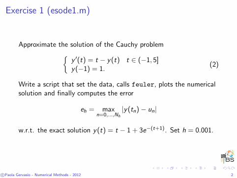
Exercise 1 (esode1.m)

Approximate the solution of the Cauchy problem

{

y ′(t) = t − y(t) t ∈ (−1, 5]y(−1) = 1.

(2)

Write a script that set the data, calls feuler, plots the numericalsolution and finally computes the error

eh = maxn=0,...,Nh

|y(tn) − un|

w.r.t. the exact solution y(t) = t − 1 + 3e−(t+1). Set h = 0.001.


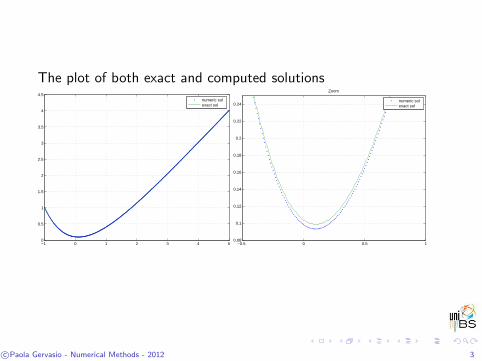
The plot of both exact and computed solutions

−1 0 1 2 3 4 50

0.5

1

1.5

2

2.5

3

3.5

4

4.5

numeric solexact sol

−0.5 0 0.5 10.08

0.1

0.12

0.14

0.16

0.18

0.2

0.22

0.24

Zoom

numeric solexact sol


Exercise 2 (esode2.m)Write a script that solves the Cauchy problem of Ex.1, withh = 1, .8, .5, .1, .05, .01, .001.For each value of h:- call the function feuler to compute [tn,un],- plot both numerical and exact solution,- compute the error

eh = maxn=0,...,Nh

|y(tn) − un|

and store these errors inside an array.

Recall that the exact solution is: y(t) = t − 1 + 3e−(t+1).Once the loop on h is terminated, plot the errors eh in logarithmicscale and verify that Forward Euler is 1st-order accurate, i.e.

∃C > 0 s.t. eh = C · h when h → 0.


Exact and numerical solutions for some values of h:

−1 0 1 2 3 4 5−1

0

1

2

3

4

5h=0.1

exact solh=1h=0.8h=0.5h=0.1

The smaller h is, the closer the numerical solution is to the exactone.The numerical solution CONVERGES to the exact one.When h → 0, maxn |un − y(tn)| → 0.


The error as a function on h is:

10−3

10−2

10−1

100

10−4

10−3

10−2

10−1

100

101

h

erro

re

Euler errorh

The two lines are parallel, then the error behaves like h whenh → 0.


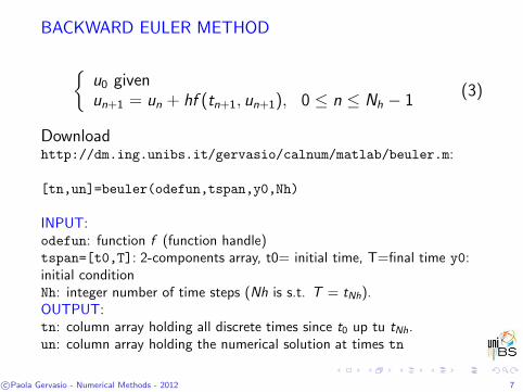
BACKWARD EULER METHOD

{

u0 givenun+1 = un + hf (tn+1, un+1), 0 ≤ n ≤ Nh − 1

(3)

Downloadhttp://dm.ing.unibs.it/gervasio/calnum/matlab/beuler.m:

[tn,un]=beuler(odefun,tspan,y0,Nh)

INPUT:odefun: function f (function handle)tspan=[t0,T]: 2-components array, t0= initial time, T=final time y0:initial conditionNh: integer number of time steps (Nh is s.t. T = tNh).OUTPUT:tn: column array holding all discrete times since t0 up tu tNh.un: column array holding the numerical solution at times tn


CRANK-NICOLSON METHOD

{

u0 givenun+1 = un + h

2[f (tn, un) + f (tn+1, un+1)], 0 ≤ n ≤ Nh − 1

(4)

Downloadhttp://dm.ing.unibs.it/gervasio/calnum/matlab/cranknic.m:

[tn,un]=cranknic(odefun,tspan,y0,Nh)

INPUT:odefun: function f (function handle)tspan=[t0,T]: 2-components array, t0= initial time, T=final time y0:initial conditionNh: integer number of time steps (Nh is s.t. T = tNh).OUTPUT:tn: column array holding all discrete times since t0 up tu tNh.

un: column array holding the numerical solution at times tn


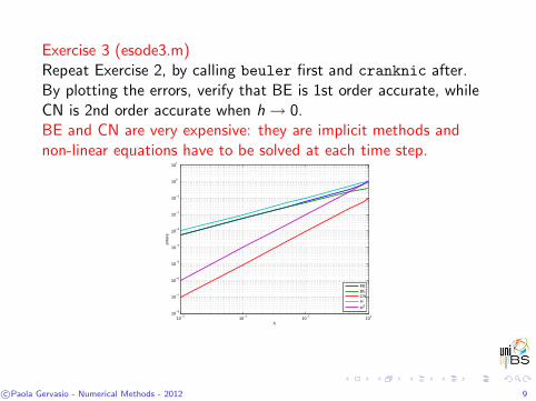
Exercise 3 (esode3.m)Repeat Exercise 2, by calling beuler first and cranknic after.By plotting the errors, verify that BE is 1st order accurate, whileCN is 2nd order accurate when h → 0.BE and CN are very expensive: they are implicit methods andnon-linear equations have to be solved at each time step.

10−3

10−2

10−1

100

10−8

10−7

10−6

10−5

10−4

10−3

10−2

10−1

100

101

h

erro

re

FEBECNH

H2


Vector Cauchy problem

{

y′(t) = F(t, y(t)) t ∈ (t0,T ]y(t0) = y0

with

y(t) =

[

y1(t)y2(t)

]

, y′(t) =

[

y ′1(t)

y ′2(t)

]

,

y0 =

[

y0,1

y0,2

]

, F(t, y(t)) =

[

F1(t, y1(t), y2(t))F2(t, y1(t), y2(t))

]

Example. Look for y1(t), y2(t) solutions of

y ′1(t) = −3y1(t) − y2(t) + sin(t) t ∈ (0, 10]

y ′2(t) = y1(t) − 5y2(t) − 2 t ∈ (0, 10]

y1(0) = y0,1 = 1, y2(0) = y0,2 = 1


Vector form of FE, BE, CNForward Euler

{

un+1 = un + hF(tn,un) n ≥ 0u0 = y0

Backward Euler{

un+1 = un + hF(tn+1,un+1) n ≥ 0u0 = y0

Crank-Nicolson{

un+1 = un + h

2 (F(tn,un) + F(tn+1,un+1)) n ≥ 0u0 = y0


All the functions work on vector problems.The initial datum y0 now must be a vector (either row or column).un is a two column arrays:

un=

y0,1 y0,2

u1,1 u2,1u1,2 u2,2

u1,Nhu2,Nh

The fucntion f=odefun(t,y) has two inputs: t (scalar) and y

(vector) and it yields the vector f with the same dimension as y.


Exercise (esodesys1) Solve the system

y ′1(t) = −3y1(t) − y2(t) + sin(t) t ∈ (0, 10]

y ′2(t) = y1(t) − 5y2(t) − 2 t ∈ (0, 10]

y1(0) = y0,1 = 1, y2(0) = y0,2 = 1

with FE and h = 1.e − 3.

0 1 2 3 4 5 6 7 8 9 10−0.5

0

0.5

1

y

1(t)

y2(t)


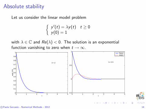
Absolute stability

Let us consider the linear model problem

{

y ′(t) = λy(t) t ≥ 0y(0) = 1

with λ ∈ C and Re(λ) < 0. The solution is an exponentialfunction vanishing to zero when t → ∞.

0 1 2 3 4 50

0.1

0.2

0.3

0.4

0.5

0.6

0.7

0.8

0.9

1

t

exp(

−2*

t)

λ=−2

0 1 2 3 4 5−0.5

0

0.5

1

t

Re(y)Im(y)

λ=−2+i


We ask that the nuemrical solution reflects the same behavior ofthe exact solution, that is it vanishes when tn → ∞.FE for the problem y ′(t) = f (t, y(t)) = λy(t) reads:

un+1 = un + hf (tn, un) = un + hλun = (1 + hλ)un

In order that un → 0 when tn → ∞.

un+1 = (1 + hλ)un

= (1 + hλ)2un−1

= .... = (1 + hλ)n+1u0

(5)


Therefore,

|un| → 0 per tn → ∞ ⇐⇒ |1 + hλ| < 1

Se λ ∈ R,

|1 + hλ| < 1 ⇐⇒ 0 < h <−2

λ

Se λ ∈ C,

|1 + hλ| < 1 ⇐⇒ 0 < h <−2Re(λ)

|λ|2.


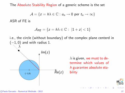
The Absolute Stability Region of a generic scheme is the set

A = {z = hλ ∈ C : un → 0 per tn → ∞}

ASR of FE is

AFE = {z = hλ ∈ C : |1 + z | < 1}

i.e., the circle (without boundary) of the complex plane centerd in(−1, 0) and with radius 1.

(−1,0) Re(z)

Im(z)

λ

λ is given, we must to de-termine which values ofh guarantee absolute sta-bility


Exercise 4 (esode4.m)

Let us consider the linear problem

{

y ′(t) = −2y(t) t ∈ [0, 10]y(0) = 1

1. Look for bounds on h such that FE is absolutely stable.2. Compute and plot the numerical solution by FE with h = 0.01,h = 0.1, h = 1, h = 2. Set h0 = −2Re(λ)

|λ|2, verify that when h < h0

the numerical scheme is absolutely stable, i.e. un → 0 whenn → ∞, while when h ≥ h0 the numerical solution providesoscillations that do not vanish when tn → ∞.3. Compute and plot the numerical solution by both BE and CNwith h = 0.01, h = 0.1, h = 1, h = 2.


FE solution: absolutely stable ∀h ∈ (0, 1)

0 2 4 6 8 100

0.2

0.4

0.6

0.8

1h=0.01

0 2 4 6 8 100

0.2

0.4

0.6

0.8

1h=0.1

0 2 4 6 8 10−1

−0.5

0

0.5

1h=1

0 2 4 6 8 10−250

−200

−150

−100

−50

0

50

100h=2


BE solution: absolutely stable ∀h > 0

0 2 4 6 8 100

0.2

0.4

0.6

0.8

1h=0.01

0 2 4 6 8 100

0.2

0.4

0.6

0.8

1h=0.1

0 2 4 6 8 100

0.2

0.4

0.6

0.8

1h=1

0 2 4 6 8 100

0.2

0.4

0.6

0.8

1h=2


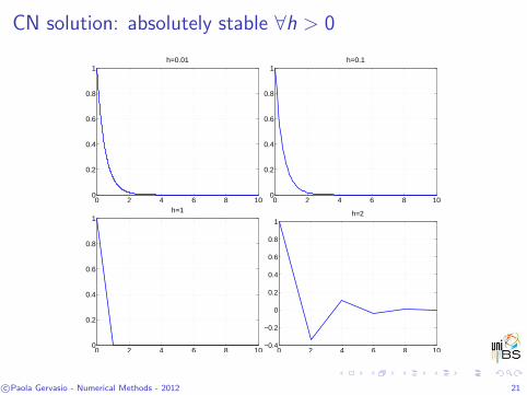
CN solution: absolutely stable ∀h > 0

0 2 4 6 8 100

0.2

0.4

0.6

0.8

1h=0.01

0 2 4 6 8 100

0.2

0.4

0.6

0.8

1h=0.1

0 2 4 6 8 100

0.2

0.4

0.6

0.8

1h=1

0 2 4 6 8 10−0.4

−0.2

0

0.2

0.4

0.6

0.8

1h=2


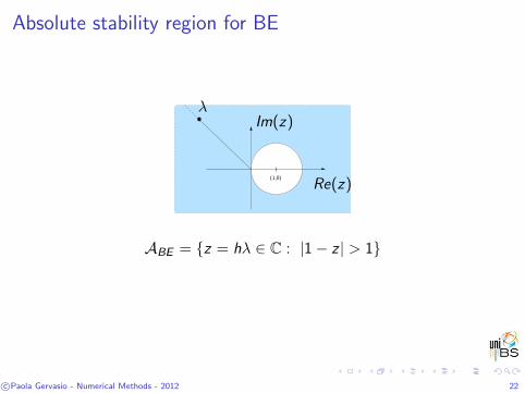
Absolute stability region for BE

(1,0)

Re(z)

Im(z)λ

ABE = {z = hλ ∈ C : |1 − z | > 1}


Absolute stability region for CN

Re(z)

Im(z)

λ

ACN = {z = hλ ∈ C : |2 + z |/|2 − z | < 1}


forward euler method - paola gervasiopaola-gervasio.unibs.it/nummeth/ode.pdf · forward euler...

Documents