Forward Motion Deblurring

Shicheng Zheng Li Xu Jiaya JiaThe Chinese University of Hong Kong

http://www.cse.cuhk.edu.hk/leojia/projects/forwarddeblur/

Abstract

We handle a special type of motion blur considering thatcameras move primarily forward or backward. Solving thistype of blur is of unique practical importance since nearlyall car, traffic and bike-mounted cameras follow out-of-plane translational motion. We start with the study of geo-metric models and analyze the difficulty of existing methodsto deal with them. We also propose a solution accountingfor depth variation. Homographies associated with differ-ent 3D planes are considered and solved for in an optimiza-tion framework. Our method is verified on several naturalimage examples that cannot be satisfyingly dealt with byprevious methods.

1. IntroductionMotion blur is one ubiquitous problem in photo taking.

Previous deblurring approaches model the degradation indifferent ways. For example, it is common to assume uni-form blur with only in-plane translation or take into accountcamera rotation. While prior models are effective on imagesproduced under their respectively defined conditions, thereare still a bunch of blurred images that find no solution inrestoration using existing techniques. Motion blur causedby out-of-plane translation falls into this set.

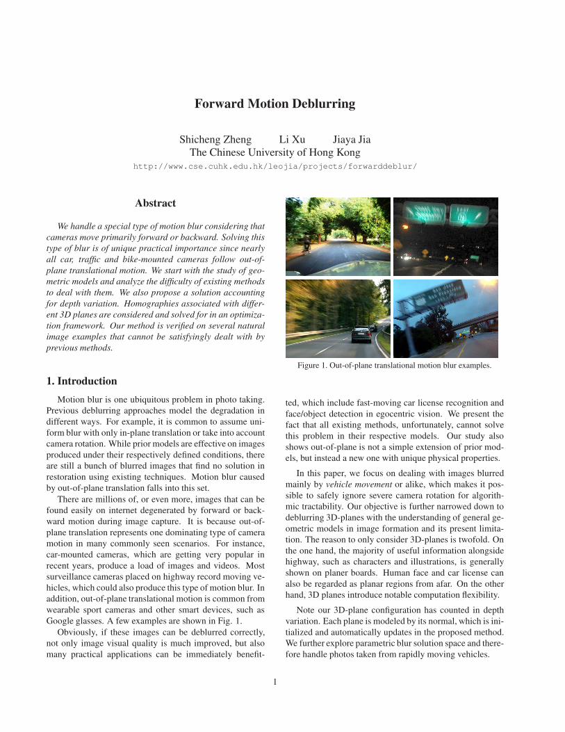
There are millions of, or even more, images that can befound easily on internet degenerated by forward or back-ward motion during image capture. It is because out-of-plane translation represents one dominating type of cameramotion in many commonly seen scenarios. For instance,car-mounted cameras, which are getting very popular inrecent years, produce a load of images and videos. Mostsurveillance cameras placed on highway record moving ve-hicles, which could also produce this type of motion blur. Inaddition, out-of-plane translational motion is common fromwearable sport cameras and other smart devices, such asGoogle glasses. A few examples are shown in Fig. 1.

Obviously, if these images can be deblurred correctly,not only image visual quality is much improved, but alsomany practical applications can be immediately benefit-

Figure 1. Out-of-plane translational motion blur examples.

ted, which include fast-moving car license recognition andface/object detection in egocentric vision. We present thefact that all existing methods, unfortunately, cannot solvethis problem in their respective models. Our study alsoshows out-of-plane is not a simple extension of prior mod-els, but instead a new one with unique physical properties.

In this paper, we focus on dealing with images blurredmainly by vehicle movement or alike, which makes it pos-sible to safely ignore severe camera rotation for algorith-mic tractability. Our objective is further narrowed down todeblurring 3D-planes with the understanding of general ge-ometric models in image formation and its present limita-tion. The reason to only consider 3D-planes is twofold. Onthe one hand, the majority of useful information alongsidehighway, such as characters and illustrations, is generallyshown on planer boards. Human face and car license canalso be regarded as planar regions from afar. On the otherhand, 3D planes introduce notable computation flexibility.

Note our 3D-plane configuration has counted in depthvariation. Each plane is modeled by its normal, which is ini-tialized and automatically updates in the proposed method.We further explore parametric blur solution space and there-fore handle photos taken from rapidly moving vehicles.

1

2. Related WorkImage deblurring finds many previous methods. State-

of-the-arts are roughly categorized to spatially-invariant andspatially-variant configurations, based on different assump-tions of the underlying blur model.

2.1. Uniform Blind Deconvolution

In uniform deblurring, Fergus et al. [2] proposed a blinddeconvolution scheme applicable to natural images. It em-ploys a variational Bayesian approach to estimate the blurkernel through marginal probability maximization. Effi-cient marginalization was later introduced in [15]. Anotherline of work is by extending the MAP framework to esti-mate latent images and blur kernels iteratively. Shan et al.[18] used adaptive regularization weights to avoid trivial so-lutions. Cho and Lee [1] predicted edges to guide kerneloptimization, which shortens running time in kernel esti-mation. Levin et al. [14] analyzed the MAP frameworkwith regard to its limitation and extensibility. Xu and Jia[24] found small structures in images could be detrimentalto kernel estimation and proposed a method to remedy thisproblem. Krishnan et al. [13] used normalized sparsity intheir MAP framework to estimate kernels. Xu et al. [26]sought an unnatural representation for blur kernel estima-tion and proposed a fast solver for restoration.

2.2. Non-Uniform Blind Deblurring

The fact that blur caused by camera shake in images areusually non-uniform motivates a series of work with methodgeneralization to model spatially variant blur. Shan et al.[19] first addressed blur caused by in-plane rotation. Tai etal. [21] used a projective model to handle spatially vari-ant blur. Whyte et al. [23, 22] used 3D rotation to modelcamera shake. In [4], the motion density function was in-troduced. In-plane translation and orthogonal rotation areused to model camera shake in another way. Hirsch et al.[6] assumed that blur is locally invariant and proposed afast non-uniform framework based on efficient filter flow[7]. Joshi et al. [8] developed a hardware solution to recordcamera shake and restore blurred images. Xu and Jia [25]used stereo images and incorporated depth into the deblur-ring framework. In addition, they proposed a hierarchicalframework for non-uniform deblurring.

2.3. Other Work

Optical aberration can be regarded as a special case ofnon-uniform blur caused by imperfection of lens. Joshi etal. [9] estimated PSFs with calibration sheets and recoveredsharp images. In [10, 16], optical blur was estimated for thelens. Schuler et al. [17] designed a set of bases to describeoptical blur and proposed a blind deconvolution method toaddress optical aberration.

3. BackgroundImage capture is the process that each element with co-

ordinate x in the camera sensor receives light from thescene X. Under homogeneous coordinates, x is denotedas (x, y, 1)T and X = (x, y, z, 1)T , where T is the trans-pose operator. Image blur typically stems from two sourcesduring exposure, i.e., camera shake and object motion. Bothtypes make the sensor element x receive light from a seriesof scene points during exposure.

In modeling the geometric formation process of camera-caused motion blur, nearly all prior methods assume con-stant scene depth z under the condition that the scene is dis-tant or front-parallel. Xu and Jia [25] took depth into con-sideration; but they need stereo images to tackle the depthproblem, which may not be applicable to single image de-blurring. Under the constant z assumption, blur image cap-ture can be regarded as a sharp image l, which is formed ina very short time interval, moves in a longer duration. Theoutput image is the weighted sum of all these transformedsharp images expressed as [23]

b =∑

i

wiPil + ε, (1)

where b denotes the blurred image and i indexes the trans-formed sharp image. All images are in the vector form inthis paper. Pi is a N ×N coefficient matrix that transformsthe latent sharp image l to li in status i, – that is, Pil = li.ε is additive noise. wi is a weight corresponding to the du-ration that the latent image stays in status i.

Actually, li and l, which are images captured with twodifferent poses, are related by a projection matrix accordingto two-view geometry [5]. Then any pixel x in l relates tothe corresponding x′ in another view as

x′ = KRK−1x + Kt/z = Hx, (2)

where R and t denote the pose of camera with a total ofsix degrees of freedom. R represents rotation around thex, y, and z axes with angles θx, θy , and θz respectively; tis translation in three directions. K is the camera intrinsicmatrix, which has focal length f measured in pixels andimage center (cx, cy) as parameters. During one shot, K isfixed due to generally constant focal length.

Eq. (2) indicates that a view can be modeled as a ho-mography warping of the latent sharp image l. By assum-ing small rotation angles as that in [23], the transformationmatrix H is written as

H = K

⎛⎝

1 −θz θy + tx/zθz 1 −θx + ty/z−θy θx 1 + tz/z

⎞⎠K−1. (3)

The problem of deblurring is actually to compute weight wi

for each pose Hi, physically corresponding to duration of

each pose. There is a mapping between homography Hi

and warping matrix Pi, where Pi is the N × N matrix andeach row is formed by the coefficient of bilinear interpola-tion. The blur kernel corresponds to w = (w1, w2, ..., wn)T

in Eq. (1), weights for each camera pose. n is the total num-ber of poses. Only the ratio of tx/z, ty/z, tz/z is requiredto parameterize homography H. Under constant depth z,the family of homography in the above blur process formsa 6D parameter space.

H and Uniform Deblurring In the uniform blur model,θx, θy , θz and tz are all set to zeros. The remaining param-eters are tx/z and ty/z in estimation. The solution spaceis thus in 2D, corresponding to shift horizontally and verti-cally in image plane.

H and Non-uniform Deblurring The full six-parametermodel is excessively complex even for non-uniform deblur-ring. Previous methods, such as those of [23, 4], tackledthis problem in 3D subspaces with only rotation or in-planerotation plus translation. Effectiveness of these methodsin approximating blur caused by typical hand-held camerashake was verified [11]. Specifically, a full homography-based model was adopted in [20] for non-blind deconvolu-tion. It is however unknown how to blindly estimate theblur kernel and latent image simultaneously, given the largesolution space.

Importance of Out-of-Plane Translation In nearly allprior deblurring methods, out-of-plane translation is ig-nored, assuming no movement orthogonal to the imageplane. As noted in Section 1, this type of translation, how-ever, is dominant in ubiquitous forward motion situations.In what follows, we discuss if motion caused by out-of-plane translation can be modeled by previous methods.

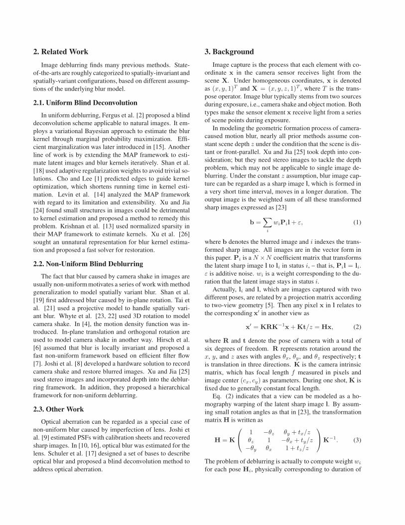
We create an image δ, which contains a few regularlyplaced dots, as shown in Fig. 2(a). This image is blurredwith forward motion only, i.e. the homography in Eq. (3) bysetting all elements to 0s except for tz . The blurred imageis shown in Fig. 2(b), visually indicating that the blur isspatially variant in a radial shape. At image center, there isalmost no blur; along the boundary, moving the camera 1cmcauses a pixel shifting 30 pixels in the 2000 × 2000 imagewhen setting scene depth z = 1 meter.

Note this is a special example used only for illustration.Our method actually handles a more general problem whereblur occurs by translation with components existing alongall axes and the motion is not necessarily perpendicular tothe image plane.

Inherent Difficulty Existing non-uniform methods, suchas those of [23, 4], cannot tackle this problem. Another fun-damental issue is on the depth value assumption. Almostall practical single-image motion deblurring methods with

(a) Dotted pattern (b) Forward blurFigure 2. Simple out-of-plane translational blur illustration.

implementation available online assume distant or front-parallel scene, which is actually not appropriate for gen-eral forward motion. It is because requiring objects com-pletely undergo translational motion perpendicular to thecamera sensor plane is overly restrictive. For example, traf-fic surveillance cameras are normally placed higher than ve-hicles or beside highway. Their viewing planes are slantedand pixels are not moving strictly forward.

In our method, we allow for varying depth and mod-eling them in a parametric form, related to 3D plane nor-mals. This strategy balances system practicality and prob-lem tractability, making the method a reasonable one forforward motion deblurring.

4. Our ModelIn our framework, points on various 3D planes are mod-

eled. Their projection on the blurred image is constrained,availing following optimization.

For a 3D plane denoted as π = (n, d), where n is thenormal vector and d is the offset to the camera center, anypoint X on the plane satisfies XT π = 0. By convention,the latent sharp image l is captured by a camera with pro-jection center at the origin. The projection matrix betweenthe world and image plane coordinates is K[I|0]. Two im-ages produced by varying camera positions are linked by ahomography as

H = K(R +tnT

d)K−1, (4)

where R refers to rotational motion and t denotes transla-tion. This representation is different from Eq. (3) for itsconsideration of varying depth. Generally, points lying on a3D plane can be with different depth values.

Because we aim to deal with images primarily producedby car or traffic surveillance cameras, the rotation matrix isset to an identity I. In addition, plane points make t/d inEq. (4) a three-variable vector, which is still represented as[tx ty tz ]T . The homography representation similar to Eq.(4) is thus

H = K

⎛⎝

1 + txn1 txn2 txn3

tyn1 1 + tyn2 tyn3

tzn1 tzn2 1 + tzn3

⎞⎠K−1 (5)

(a)

(b) (c) (d)

=+w3

++w2w1

x

y

z(1,0,0)

x

y

z

x

y

z (0,0,1)

(0,1,0)

l1 l2 l3

=+w3

++w2w1

l1 l2 l3

=+w3

++w2w1

l1 l2 l3

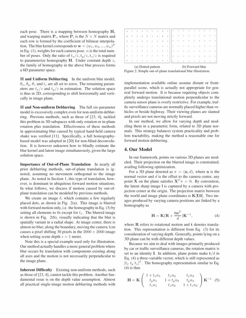
Figure 3. Demonstration of homography bases considering three special normals. (a) Natural images generally contain planar surfaces. (b)Corresponding forward motion blurred image to (a). (c) Three special cases. Each blurred surface is a weighed sum of a few transformedplanes li defined in Eq. (1). (d) Resulting blurred planes.

where n = (n1, n2, n3)T in 3D space. Given tx, ty , tz andn, we can uniquely determine a homography, which alsocorresponds to a N ×N warping matrix P described in Eq.(1) – one P maps to one homography H. In this regard, wetransform originally very difficult whole-image deblurringto a plane-wise tractable problem, counting in non-frontal3D planes.

Homography Space Eq. (5) indicates that one ho-mography, or the corresponding camera pose, is deter-mined uniquely by vectors t = (tx, ty, tz)T and n =(n1, n2, n3)T with a total of 6 variables (or 5 of them ifn is normalized). We thus propose constructing 3D homog-raphy space t = (tx, ty, tz)T and sample each tx, ty , andtz discretely to predefine a few camera poses. The normaln, contrarily, is set as another parameter updated in passes.Put differently, our method uses a series of discrete Hn

i topresent the original continuous homography space, each ho-mography or status is determined by a corresponding n andby a pose ti indexed by i.

Fig. 3 shows an example for demonstrating the specialtyof forward motion blur. We use the dotted pattern to visu-alize point trajectories and homography basis, which makethis kind of blur formation easy to comprehend. (a) is toshow that forward motion blurred images, such as that in(b), can generally find a few planes.

We then consider three special cases with plane normalsn being respectively (1, 0, 0), (0, 1, 0), and (0, 0, 1), as il-lustrated in the three rows in Fig. 3(c). Previous methods,even for non-uniform deblurring, mostly consider the casen = (0, 0, 1), whereas our method handles all of them aswell as planes with all non-zero elements in normal n.

+ + =

b

l

w1 1l...w2 2l w3 3l

...

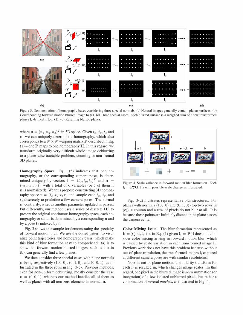
Figure 4. Scale variance in forward motion blur formation. Eachli = Pn

i Gil is with possible scale change as illustrated.

Fig. 3(d) illustrates representative blur structures. Forplanes with normals (1, 0, 0) and (0, 1, 0) (top two rows in(c)), a column and a row of pixels do not blur at all. It isbecause these points are infinitely distant or the plane passesthe camera center.

Color Mixing Issue The blur formation represented asb =

∑i wili + ε in Eq. (1) given li = Pn

i l does not con-sider color mixing arising in forward motion blur, whichis caused by scale variation in each transformed image li.Previous work does not have this problem because withoutout-of-plane translation, the transformed images li capturedat different camera poses are with similar resolutions.

Note in out-of-plane motion, a similarity transform foreach li is resulted in, which changes image scales. In thisregard, one pixel in the blurred image is not a summation (orintegration) of a few isolated unblurred pixels, but rather acombination of several patches, as illustrated in Fig. 4.

We generally take the reference image l as the one withthe highest resolution among all. It is with tz = 0 and allother li are with tz < 0, corresponding to down-scaled ver-sions of l. To practically model the resulting blurred imageb and avoid aliasing, we regard b as the sum of latent im-ages li blurred by Gaussian filter, whose standard deviationis determined by tz corresponding to each li. Typically,we set the standard deviation of Gaussian in [0.1, 0.5] andlinearly interpolate pixels according to tz . This process issimilar to image sampling, but with different convolutionkernels. The final blur model is finely expressed as

b =∑

i

wiPni Gil + ε, (6)

where Gi is a BTTB (block-Toeplitz with Toeplitz-block)matrix representing the Gaussian blur kernel in a matrixform. Our final li is expressed as Pn

i Gil. We describein the next section our deblurring algorithm based on thismodel.

5. Forward Motion DeblurringThe model in Eq. (6) depends on three sets of variables,

namely w, l, and normal n. Solving for w and l with a fixedn corresponds to a non-uniform deblurring problem. We re-sort to alternating minimization to estimate them iteratively.

5.1. Kernel and Image Restoration

The first sub-problem is to fix n and estimate w and l,which is referred to as blind deconvolution. w is knownas blur kernel, since it records the duration of each camerapose, conceptually similar to 2D uniform blur PSFs.

One nice property of Eq. (6) is the bilinear form it takes,since Gi is a linear translation-invariant operator. We thuswrite ∑

i

wiPni Gil = Bnl = Anw, (7)

where Bn =∑

i wiPni Gi and coli(An) = Pn

i Gil. coli(·)returns the i-th column of matrix An. w is the vec-tor (w1, w2, ...)T . We define the quadratic data cost term‖b− ∑

i wiPni Gil‖2 following tradition.

Kernel Update We update w by solving energy function

E(w) = ‖Anw − b‖2 + γ‖w‖2,

s.t.∑

i wi = 1 (8)

where γ controls the smoothing strength. The constraint∑i wi = 1 is for energy conservation. The objective func-

tion is quadratic with respect to w. However, directly solv-ing Eq. (8) involves inversion of An, which is computation-ally expensive and unstable. We use the local uniform as-sumption [6] for acceleration considering smoothly chang-ing blur kernels under depth variation on 3D planes.

Conjugate gradient (CG) is employed to update w in thisstep. Normalization to make

∑i wi = 1 is applied after the

result of w is obtained.

Image Update In uniform deblurring, extra steps withshock filter [1] are generally employed to help kernel es-timation. Recent development [13, 26] shows that sparsity-pursuit regularization can replace these ad-hoc steps andgenerate similar or better representations in a unified energyminimization framework. Speed of convergence and resultquality can both be enhanced [26]. Our method follows thisline and similarly adopts the high-sparsity form as

E(l) = ‖Bnl − b‖2 + λφ(∇l), (9)

where φ(∇l) is the high-sparsity regularization term on im-age gradients, approximating L0-norm (defined in [26]). λis a weight. The scale-invariant property of L0-sparsity isvital to guide blur kernel estimation. We do not performshock filtering and instead use the efficient solver in [26]for optimization.

The image and kernel estimates are updated iteratively ina multi-scale scheme [23]. It converges quickly. The finallyrestored image, based on the kernel result, is produced byoptimization incorporating a natural image hyper-Laplacian[12] prior. Other image priors, such as that in [27], can alsobe adopted.

5.2. Normal Refinement

The above method depends on a specified normal n. Wewill discuss in Section 6 the way to initialize it. In whatfollows, we parameterize n for its refinement.

A plane normal is parameterized in the spherical coordi-nate system as

n = (n1, n2, n3)T = (cosα sinβ, sin α sin β, cosβ)T , (10)

where α and β are polar and azimuthal angles respectively.With the constraint that each n is normalized, the number ofparameters is actually 2. The energy function with respectto n is

E(n) = ‖∑

i

wiPni Gil − b‖2. (11)

The derivatives of E(n) are non-linear. Gradient descent[3], such as Matlab fminunc function, fails to produce rea-sonable results in practice.

Our strategy to update the normal estimate is samplingand testing. Given the input normal specified by angles α0

and β0, we update them within α0±15◦ and β0±15◦, witheach interval 5◦. We have therefore a total of 49 candidates,which are fed into Eq. (11) for evaluation. The one withthe smallest energy is kept as the new normal in the currentpass. This process guarantees energy decreasing.

After the normal is updated, we solve for w and l again.Only 3 passes are enough to obtain a reasonable result inour experiments.

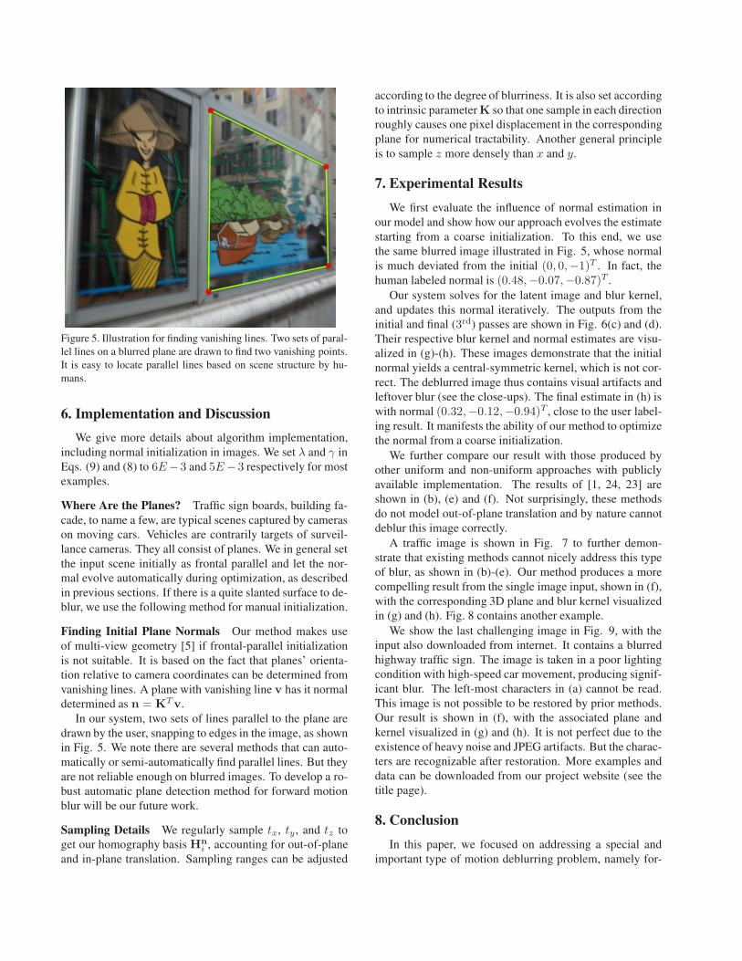
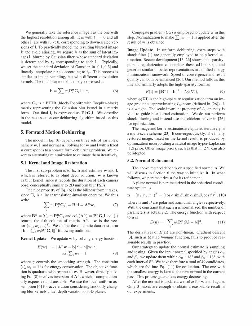
Figure 5. Illustration for finding vanishing lines. Two sets of paral-lel lines on a blurred plane are drawn to find two vanishing points.It is easy to locate parallel lines based on scene structure by hu-mans.

6. Implementation and DiscussionWe give more details about algorithm implementation,

including normal initialization in images. We set λ and γ inEqs. (9) and (8) to 6E−3 and 5E−3 respectively for mostexamples.

Where Are the Planes? Traffic sign boards, building fa-cade, to name a few, are typical scenes captured by camerason moving cars. Vehicles are contrarily targets of surveil-lance cameras. They all consist of planes. We in general setthe input scene initially as frontal parallel and let the nor-mal evolve automatically during optimization, as describedin previous sections. If there is a quite slanted surface to de-blur, we use the following method for manual initialization.

Finding Initial Plane Normals Our method makes useof multi-view geometry [5] if frontal-parallel initializationis not suitable. It is based on the fact that planes’ orienta-tion relative to camera coordinates can be determined fromvanishing lines. A plane with vanishing line v has it normaldetermined as n = KTv.

In our system, two sets of lines parallel to the plane aredrawn by the user, snapping to edges in the image, as shownin Fig. 5. We note there are several methods that can auto-matically or semi-automatically find parallel lines. But theyare not reliable enough on blurred images. To develop a ro-bust automatic plane detection method for forward motionblur will be our future work.

Sampling Details We regularly sample tx, ty , and tz toget our homography basis Hn

i , accounting for out-of-planeand in-plane translation. Sampling ranges can be adjusted

according to the degree of blurriness. It is also set accordingto intrinsic parameter K so that one sample in each directionroughly causes one pixel displacement in the correspondingplane for numerical tractability. Another general principleis to sample z more densely than x and y.

7. Experimental ResultsWe first evaluate the influence of normal estimation in

our model and show how our approach evolves the estimatestarting from a coarse initialization. To this end, we usethe same blurred image illustrated in Fig. 5, whose normalis much deviated from the initial (0, 0,−1)T . In fact, thehuman labeled normal is (0.48,−0.07,−0.87)T .

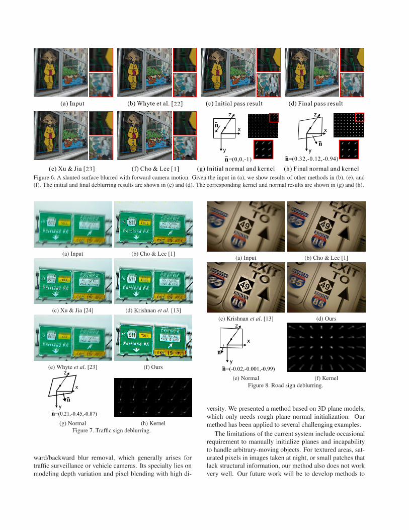
Our system solves for the latent image and blur kernel,and updates this normal iteratively. The outputs from theinitial and final (3rd) passes are shown in Fig. 6(c) and (d).Their respective blur kernel and normal estimates are visu-alized in (g)-(h). These images demonstrate that the initialnormal yields a central-symmetric kernel, which is not cor-rect. The deblurred image thus contains visual artifacts andleftover blur (see the close-ups). The final estimate in (h) iswith normal (0.32,−0.12,−0.94)T , close to the user label-ing result. It manifests the ability of our method to optimizethe normal from a coarse initialization.

We further compare our result with those produced byother uniform and non-uniform approaches with publiclyavailable implementation. The results of [1, 24, 23] areshown in (b), (e) and (f). Not surprisingly, these methodsdo not model out-of-plane translation and by nature cannotdeblur this image correctly.

A traffic image is shown in Fig. 7 to further demon-strate that existing methods cannot nicely address this typeof blur, as shown in (b)-(e). Our method produces a morecompelling result from the single image input, shown in (f),with the corresponding 3D plane and blur kernel visualizedin (g) and (h). Fig. 8 contains another example.

We show the last challenging image in Fig. 9, with theinput also downloaded from internet. It contains a blurredhighway traffic sign. The image is taken in a poor lightingcondition with high-speed car movement, producing signif-icant blur. The left-most characters in (a) cannot be read.This image is not possible to be restored by prior methods.Our result is shown in (f), with the associated plane andkernel visualized in (g) and (h). It is not perfect due to theexistence of heavy noise and JPEG artifacts. But the charac-ters are recognizable after restoration. More examples anddata can be downloaded from our project website (see thetitle page).

8. ConclusionIn this paper, we focused on addressing a special and

important type of motion deblurring problem, namely for-

(a) Input

(e) Xu & Jia [ ]23

(b) Whyte et al. [ ]22

(f) Cho & Lee [ ]1

n

=(0,0,-1)n =(0.32,-0.12,-0.94)

n

x

y

z

x

y

z

n

(g) Initial normal and kernel

(c) Initial pass result (d) Final pass result

(h) Final normal and kernel

Figure 6. A slanted surface blurred with forward camera motion. Given the input in (a), we show results of other methods in (b), (e), and(f). The initial and final deblurring results are shown in (c) and (d). The corresponding kernel and normal results are shown in (g) and (h).

(a) Input (b) Cho & Lee [1]

(c) Xu & Jia [24] (d) Krishnan et al. [13]

(e) Whyte et al. [23] (f) Oursz

n=(0 21,-0.45,-0.87).

n

y

x

(g) Normal (h) KernelFigure 7. Traffic sign deblurring.

ward/backward blur removal, which generally arises fortraffic surveillance or vehicle cameras. Its specialty lies onmodeling depth variation and pixel blending with high di-

(a) Input (b) Cho & Lee [1]

(c) Krishnan et al. [13] (d) Oursz

n=(-0 02,-0.001,-0.99).

n

y

x

(e) Normal (f) KernelFigure 8. Road sign deblurring.

versity. We presented a method based on 3D plane models,which only needs rough plane normal initialization. Ourmethod has been applied to several challenging examples.

The limitations of the current system include occasionalrequirement to manually initialize planes and incapabilityto handle arbitrary-moving objects. For textured areas, sat-urated pixels in images taken at night, or small patches thatlack structural information, our method also does not workvery well. Our future work will be to develop methods to

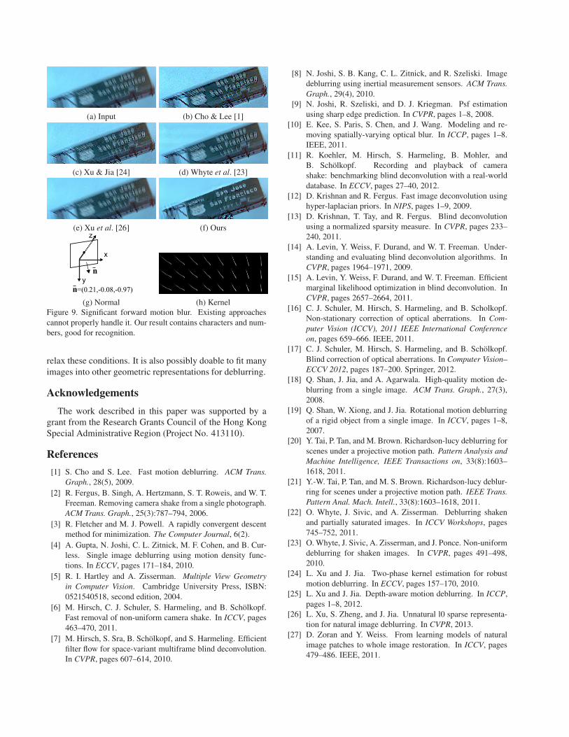
(a) Input (b) Cho & Lee [1]

(c) Xu & Jia [24] (d) Whyte et al. [23]

(e) Xu et al. [26] (f) Oursz

n=(0 21,-0.08,-0.97).

n

y

x

(g) Normal (h) KernelFigure 9. Significant forward motion blur. Existing approachescannot properly handle it. Our result contains characters and num-bers, good for recognition.

relax these conditions. It is also possibly doable to fit manyimages into other geometric representations for deblurring.

AcknowledgementsThe work described in this paper was supported by a

grant from the Research Grants Council of the Hong KongSpecial Administrative Region (Project No. 413110).

References[1] S. Cho and S. Lee. Fast motion deblurring. ACM Trans.

Graph., 28(5), 2009.[2] R. Fergus, B. Singh, A. Hertzmann, S. T. Roweis, and W. T.

Freeman. Removing camera shake from a single photograph.ACM Trans. Graph., 25(3):787–794, 2006.

[3] R. Fletcher and M. J. Powell. A rapidly convergent descentmethod for minimization. The Computer Journal, 6(2).

[4] A. Gupta, N. Joshi, C. L. Zitnick, M. F. Cohen, and B. Cur-less. Single image deblurring using motion density func-tions. In ECCV, pages 171–184, 2010.

[5] R. I. Hartley and A. Zisserman. Multiple View Geometryin Computer Vision. Cambridge University Press, ISBN:0521540518, second edition, 2004.

[6] M. Hirsch, C. J. Schuler, S. Harmeling, and B. Scholkopf.Fast removal of non-uniform camera shake. In ICCV, pages463–470, 2011.

[7] M. Hirsch, S. Sra, B. Scholkopf, and S. Harmeling. Efficientfilter flow for space-variant multiframe blind deconvolution.In CVPR, pages 607–614, 2010.

[8] N. Joshi, S. B. Kang, C. L. Zitnick, and R. Szeliski. Imagedeblurring using inertial measurement sensors. ACM Trans.Graph., 29(4), 2010.

[9] N. Joshi, R. Szeliski, and D. J. Kriegman. Psf estimationusing sharp edge prediction. In CVPR, pages 1–8, 2008.

[10] E. Kee, S. Paris, S. Chen, and J. Wang. Modeling and re-moving spatially-varying optical blur. In ICCP, pages 1–8.IEEE, 2011.

[11] R. Koehler, M. Hirsch, S. Harmeling, B. Mohler, andB. Scholkopf. Recording and playback of camerashake: benchmarking blind deconvolution with a real-worlddatabase. In ECCV, pages 27–40, 2012.

[12] D. Krishnan and R. Fergus. Fast image deconvolution usinghyper-laplacian priors. In NIPS, pages 1–9, 2009.

[13] D. Krishnan, T. Tay, and R. Fergus. Blind deconvolutionusing a normalized sparsity measure. In CVPR, pages 233–240, 2011.

[14] A. Levin, Y. Weiss, F. Durand, and W. T. Freeman. Under-standing and evaluating blind deconvolution algorithms. InCVPR, pages 1964–1971, 2009.

[15] A. Levin, Y. Weiss, F. Durand, and W. T. Freeman. Efficientmarginal likelihood optimization in blind deconvolution. InCVPR, pages 2657–2664, 2011.

[16] C. J. Schuler, M. Hirsch, S. Harmeling, and B. Scholkopf.Non-stationary correction of optical aberrations. In Com-puter Vision (ICCV), 2011 IEEE International Conferenceon, pages 659–666. IEEE, 2011.

[17] C. J. Schuler, M. Hirsch, S. Harmeling, and B. Scholkopf.Blind correction of optical aberrations. In Computer Vision–ECCV 2012, pages 187–200. Springer, 2012.

[18] Q. Shan, J. Jia, and A. Agarwala. High-quality motion de-blurring from a single image. ACM Trans. Graph., 27(3),2008.

[19] Q. Shan, W. Xiong, and J. Jia. Rotational motion deblurringof a rigid object from a single image. In ICCV, pages 1–8,2007.

[20] Y. Tai, P. Tan, and M. Brown. Richardson-lucy deblurring forscenes under a projective motion path. Pattern Analysis andMachine Intelligence, IEEE Transactions on, 33(8):1603–1618, 2011.

[21] Y.-W. Tai, P. Tan, and M. S. Brown. Richardson-lucy deblur-ring for scenes under a projective motion path. IEEE Trans.Pattern Anal. Mach. Intell., 33(8):1603–1618, 2011.

[22] O. Whyte, J. Sivic, and A. Zisserman. Deblurring shakenand partially saturated images. In ICCV Workshops, pages745–752, 2011.

[23] O. Whyte, J. Sivic, A. Zisserman, and J. Ponce. Non-uniformdeblurring for shaken images. In CVPR, pages 491–498,2010.

[24] L. Xu and J. Jia. Two-phase kernel estimation for robustmotion deblurring. In ECCV, pages 157–170, 2010.

[25] L. Xu and J. Jia. Depth-aware motion deblurring. In ICCP,pages 1–8, 2012.

[26] L. Xu, S. Zheng, and J. Jia. Unnatural l0 sparse representa-tion for natural image deblurring. In CVPR, 2013.

[27] D. Zoran and Y. Weiss. From learning models of naturalimage patches to whole image restoration. In ICCV, pages479–486. IEEE, 2011.