foundations of cryptography 89-856 - biuu.cs.biu.ac.il/~lindell/89-856/complete-89-856.pdf · the...
TRANSCRIPT
Foundations of Cryptography89-856
Yehuda Lindell
Dept. of Computer Science
Bar-Ilan University, Israel.
April 26, 2010

c© Copyright 2005 by Yehuda Lindell.Permission to make copies of part or all of this work for personal or classroom use is grantedwithout fee provided that copies are not made or distributed for profit or commercial advantageand that new copies bear this notice and the full citation on the first page. Abstracting with creditis permitted.
Abstract and Course Syllabus
Abstract
In this course, we will study the theoretical foundations of modern cryptography. Thefocus of the course is to understand what cryptographic problems can be solved, andunder what assumptions. Most of the course will follow the presentation of the relevantmaterial in Oded Goldreich’s books on the foundations of cryptography [5, 6]. Thecourse obligations include exercises and a final exam. In addition, there will be readingassignments on important material that we will not have time to cover in class.
Course Syllabus
1. (a) Introduction and background: a rigorous approach to cryptography, the focus ofthe foundations of cryptography, background on the computational model
(b) One-way functions I: definitions of strong and weak one-way functions, candidates
2. One-way functions II: strong versus weak one-way functions, definitions of collections ofone-way functions and trapdoor permutations, definition of hard-core predicates, preliminariesfor Goldreich-Levin
3. Hard-core predicates: proof of existence (the Goldreich-Levin hardcore predicate).
4. Computational indistinguishability and pseudorandomness: definition of computa-tional indistinguishability, multiple sample theorem, definition of pseudorandomness, defini-tion and construction of pseudorandom generators, extending the expansion factor of pseu-dorandom generators
5. Pseudorandomness II: definition of pseudorandom functions, construction of pseudoran-dom functions from pseudorandom generators
6. Zero knowledge I: motivation, interactive proofs - definitions, perfect zero-knowledge prooffor Diffie-Hellman tuples
7. Zero knowledge II: commitment schemes, zero-knowledge proofs for all languages in NP
8. Zero knowledge III: proofs of knowledge, non-interactive zero-knowledge (may be skipped)
9. Encryption schemes I: definitions – indistinguishability, semantic security and their equiv-alence, security under multiple encryptions.
10. Encryption schemes II: constructions of secure private-key and public-key encryptionschemes; definitions of security for more powerful adversaries
1
2
11. Digital signatures I: definitions, constructions
12. Digital signatures II: constructions, constructions of hash functions
13. Secure multiparty computation: motivation, definitions, semi-honest oblivious transfer,the GMW construction
A word about references. We do not provide full references for all of the material that wepresent. To make things worse, our choice of what to cite and what not to cite is arbitrary. Morecomplete citations can be found in [5] and [6] in the “historical notes” section at the end of eachchapter.
Course Text Books
1. O. Goldreich. Foundations of Cryptography: Volume 1 – Basic Tools. Cambridge UniversityPress, 2001.
2. O. Goldreich. Foundations of Cryptography: Volume 2 – Basic Applications. CambridgeUniversity Press, 2004.
Contents
1 Introduction and One-Way Functions 5
1.1 Introduction . . . . . . . . . . . . . . . . . . . . . . . . . . . . . . . . . . . . . . . . . 5
1.1.1 Preliminaries . . . . . . . . . . . . . . . . . . . . . . . . . . . . . . . . . . . . 6
1.2 Computational Difficulty – One-Way Functions . . . . . . . . . . . . . . . . . . . . . 8
1.2.1 One-Way Functions – Definition . . . . . . . . . . . . . . . . . . . . . . . . . 8
1.2.2 Weak One-Way Functions . . . . . . . . . . . . . . . . . . . . . . . . . . . . . 9
1.2.3 Candidates . . . . . . . . . . . . . . . . . . . . . . . . . . . . . . . . . . . . . 10
1.3 Strong Versus Weak One-Way Functions . . . . . . . . . . . . . . . . . . . . . . . . . 10
1.3.1 Weak One-Way Functions Are Not Necessarily Strong . . . . . . . . . . . . . 10
2 One-Way Functions (continued) 13
2.1 Strong Versus Weak One-Way Functions . . . . . . . . . . . . . . . . . . . . . . . . . 13
2.1.1 Equivalence of Weak and Strong One-Way Functions . . . . . . . . . . . . . . 13
2.2 Collections of One-Way Functions . . . . . . . . . . . . . . . . . . . . . . . . . . . . 13
2.3 Trapdoor One-Way Permutations . . . . . . . . . . . . . . . . . . . . . . . . . . . . . 14
2.4 Hard-Core Predicates . . . . . . . . . . . . . . . . . . . . . . . . . . . . . . . . . . . 15
2.5 Hard-Core Predicates for Any One-Way Function . . . . . . . . . . . . . . . . . . . . 16
2.5.1 Preliminaries – Markov and Chebyshev Inequalities . . . . . . . . . . . . . . . 16
3 Hard-Core Predicates for Any One-Way Function 19
3.1 Proof of the Goldreich-Levin Hard-Core Predicate [8] . . . . . . . . . . . . . . . . . . 19
4 Computational Indistinguishability & Pseudorandomness 23
4.1 Computational Indistinguishability . . . . . . . . . . . . . . . . . . . . . . . . . . . . 23
4.1.1 Multiple Samples . . . . . . . . . . . . . . . . . . . . . . . . . . . . . . . . . . 24
4.1.2 Pseudorandomness . . . . . . . . . . . . . . . . . . . . . . . . . . . . . . . . . 27
4.2 Pseudorandom Generators . . . . . . . . . . . . . . . . . . . . . . . . . . . . . . . . . 27
4.2.1 Pseudorandom Generators from One-Way Permutations . . . . . . . . . . . . 28
4.2.2 Increasing the Expansion Factor . . . . . . . . . . . . . . . . . . . . . . . . . 29
4.2.3 Pseudorandom Generators and One-Way Functions . . . . . . . . . . . . . . . 30
5 Pseudorandom Functions and Zero Knowledge 31
5.1 Pseudorandom Functions . . . . . . . . . . . . . . . . . . . . . . . . . . . . . . . . . 31
5.1.1 Definitions . . . . . . . . . . . . . . . . . . . . . . . . . . . . . . . . . . . . . 31
5.2 Constructions of Pseudorandom Functions . . . . . . . . . . . . . . . . . . . . . . . . 32
5.2.1 Applications . . . . . . . . . . . . . . . . . . . . . . . . . . . . . . . . . . . . 34
5.3 Zero-Knowledge Interactive Proof Systems . . . . . . . . . . . . . . . . . . . . . . . . 34
3
4 CONTENTS
5.3.1 Interactive Proofs . . . . . . . . . . . . . . . . . . . . . . . . . . . . . . . . . 36
6 Zero-Knowledge Proofs and Perfect Zero-Knowledge 39
6.1 Zero Knowledge Proofs – Definitions . . . . . . . . . . . . . . . . . . . . . . . . . . . 39
6.2 Perfect Zero-Knowledge for Diffie-Hellman Tuples . . . . . . . . . . . . . . . . . . . . 40
7 Zero-Knowledge for all NP 45
7.1 Commitment Schemes . . . . . . . . . . . . . . . . . . . . . . . . . . . . . . . . . . . 45
7.2 Zero-Knowledge for the Language 3COL . . . . . . . . . . . . . . . . . . . . . . . . . 47
7.3 Zero-Knowledge for every Language L ∈ NP . . . . . . . . . . . . . . . . . . . . . . 51
7.4 More on Zero-Knowledge . . . . . . . . . . . . . . . . . . . . . . . . . . . . . . . . . 52
8 Proofs of Knowledge and Non-Interactive Zero Knowledge 53
9 Encryption Schemes I 55
9.1 Definitions of Security . . . . . . . . . . . . . . . . . . . . . . . . . . . . . . . . . . . 55
9.1.1 Semantic Security . . . . . . . . . . . . . . . . . . . . . . . . . . . . . . . . . 56
9.1.2 Indistinguishability . . . . . . . . . . . . . . . . . . . . . . . . . . . . . . . . . 57
9.1.3 Equivalence of the Definitions . . . . . . . . . . . . . . . . . . . . . . . . . . . 58
9.2 Security Under Multiple Encryptions . . . . . . . . . . . . . . . . . . . . . . . . . . . 59
9.2.1 Multiple Encryptions in the Public-Key Setting . . . . . . . . . . . . . . . . . 60
9.2.2 Multiple Encryptions in the Private-Key Setting . . . . . . . . . . . . . . . . 61
10 Encryption Schemes II 63
10.1 Constructing Secure Encryption Schemes . . . . . . . . . . . . . . . . . . . . . . . . 63
10.1.1 Private-Key Encryption Schemes . . . . . . . . . . . . . . . . . . . . . . . . . 63
10.1.2 Public-Key Encryption Schemes . . . . . . . . . . . . . . . . . . . . . . . . . 64
10.2 Secure Encryption for Active Adversaries . . . . . . . . . . . . . . . . . . . . . . . . 66
10.2.1 Definitions . . . . . . . . . . . . . . . . . . . . . . . . . . . . . . . . . . . . . 66
10.2.2 Constructions . . . . . . . . . . . . . . . . . . . . . . . . . . . . . . . . . . . . 68
11 Digital Signatures I 69
11.1 Defining Security for Signature Schemes . . . . . . . . . . . . . . . . . . . . . . . . . 69
11.2 Length-Restricted Signatures . . . . . . . . . . . . . . . . . . . . . . . . . . . . . . . 70
11.2.1 From Length-Restricted to Full-Fledged Signature Schemes . . . . . . . . . . 70
11.2.2 Collision-Resistant Hash Functions and Extending Signatures . . . . . . . . . 72
11.2.3 Constructing Collision-Resistant Hash Functions . . . . . . . . . . . . . . . . 74
12 Digital Signatures II 75
12.1 Minimal Assumptions for Digital Signatures . . . . . . . . . . . . . . . . . . . . . . . 75
12.2 Secure One-Time Signature Schemes . . . . . . . . . . . . . . . . . . . . . . . . . . . 75
12.2.1 Length-Restricted One-Time Signature Schemes . . . . . . . . . . . . . . . . 76
12.2.2 General One-Time Signature Schemes . . . . . . . . . . . . . . . . . . . . . . 76
12.3 Secure Memory-Dependent Signature Schemes . . . . . . . . . . . . . . . . . . . . . . 77
12.4 Secure Memoryless Signature Schemes . . . . . . . . . . . . . . . . . . . . . . . . . . 79
12.5 Removing the Need for Collision-Resistant Hash Functions . . . . . . . . . . . . . . . 80
CONTENTS 5
13 Secure Multiparty Computation 8313.1 Motivation . . . . . . . . . . . . . . . . . . . . . . . . . . . . . . . . . . . . . . . . . 8313.2 Definition of Security . . . . . . . . . . . . . . . . . . . . . . . . . . . . . . . . . . . . 8713.3 Oblivious Transfer . . . . . . . . . . . . . . . . . . . . . . . . . . . . . . . . . . . . . 8913.4 Constructions of Secure Protocols . . . . . . . . . . . . . . . . . . . . . . . . . . . . . 90
13.4.1 Security Against Semi-Honest Adversaries . . . . . . . . . . . . . . . . . . . . 9013.4.2 The GMW Compiler . . . . . . . . . . . . . . . . . . . . . . . . . . . . . . . . 91
References 93

6 CONTENTS
Lecture 1
Introduction and One-Way Functions
1.1 Introduction
In this course, we will study the theoretical foundations of cryptography. The main questionswe will ask are what cryptographic problems can be solved and under what assumptions. Thusthe main focus of the course is the presentation of “feasibility results” (i.e., proofs that a certaincryptographic task can be realized under certain assumptions). We will typically not relate to issuesof efficiency (beyond equating efficiency with polynomial-time). There are a number of significantdifferences between this course and its prerequisite “Introduction to Cryptography” (89-656) givenlast semester:
1. First, our presentation here will be rigorous, and so we will only present constructions thathave been proven secure.
2. Second, we will not begin with cryptographic applications like encryption and signatures,but will rather conclude with them. Rather, we start by studying one-way functions andtheir variants, and then show how different cryptographic primitives can be built from these.(Continuing the analogy of “foundations”, we begin by building from the foundations and up,rather than starting with applications and working down to show how they can be securelyrealized.)
3. Third, the aim of the course is to provide the students with a deep understanding of howsecure cryptographic solutions are achieved, rather than with a basic understanding of theimportant concepts and constructions.1 Thus, we will cover far fewer topics in this course.
We note that the need for a rigorous approach in cryptography is especially strong. First, intuitiveand heuristic arguments of security have been known to fail dismally when it comes to cryptography.Personally, my intuition has failed me many times. (I therefore do not believe anything until I havea full proof, and then I start thinking that it may be correct.) Second, in contrast to many otherfields, the security of a cryptographic construction cannot be tested empirically. (By running aseries of tests, you can see if something works under “many” conditions. However, such testsare of no help in seeing if a protocol can or cannot be maliciously attacked.) Finally, we note
* Lecture notes for a graduate course in the theory of cryptography. Yehuda Lindell, Bar-Ilan University, Israel, 2005.My intention here is not at all to belittle the importance and place of the introductory course. Rather, the aimis different. I view the aim of the introductory course to provide students with an understanding of cryptographicproblems and solutions that will guide them as consumers of cryptography. In contrast, the aim of this course is tobe a first step on the way to learning how to build cryptographic solutions and prove them secure.
7
8 LECTURE 1. INTRODUCTION AND ONE-WAY FUNCTIONS
that the potential damage of implementing an insecure solution is often too great to warrant thechance. (In this way, cryptography differs from algorithms. A rigorous approach to algorithmsis also important. However, heuristic solutions that almost always provide optimal solutions areoften what is needed. In contrast, a cryptographic protocol that prevents most attacks is worthless,because an adversary can maliciously direct its attack at the weakest link.)
1.1.1 Preliminaries
We assume familiarity with complexity classes like P, NP, BPP and P/poly. In general, weequate the notion of “efficient computation” with probabilistic polynomial-time. Thus, adversariesare assumed to be probabilistic polynomial-time Turing machines. (Recall that a Turing machineM runs in polynomial-time if there exists a single polynomial p(·) such that for every input x,the computation of M(x) halts within p(|x|) steps.) We will sometimes also consider non-uniformadversaries. Such an adversary can be modelled in one of two equivalent ways:
1. Turing machine with advice: In this formalization, a non-uniform machine is a pair (M,a)where M is a two-input polynomial-time Turing machine and a is an infinite sequence ofstrings such that for every n ∈ N, |an| = poly(n).2 The string an is the advice that Mreceives upon inputs of length n (note that for all inputs of length n, M receives the sameadvice).
2. Families of polynomial-size circuits: In this formalization, a non-uniform “machine” is repre-sented by an infinite sequence (or family) of Boolean circuits C = (C1, C2, . . .) such that forevery n ∈ N, |Cn| = poly(n). Then, the computation upon input x is given by C|x|(x). Wenote that the size of a circuit is given by the number of edges that it has, and that there is asingle polynomial that bounds the size of all circuits in the family.
Recall that BPP ⊆ P/poly. Therefore, for many tasks (like deciding a language or carrying out awell-defined adversarial attack), it holds that anything that a probabilistic polynomial-time machinecan do, a non-uniform polynomial-time machine can also do. Thus, non-uniform adversaries arestronger than probabilistic polynomial-time ones. It is not clear whether adversaries should bemodelled as probabilistic polynomial-time or non-uniform polynomial-time (or whether this makesany difference). The tradeoff between them, however, is clear: security guarantees against non-uniform adversaries are stronger, but almost always rely on stronger hardness assumptions (see“intractability assumptions” below). Another important point to make is that proofs of securityfor probabilistic polynomial-time adversaries hold also for non-uniform polynomial-time adversaries.Therefore, “uniform” proofs of security are preferable (where they are known).
Negligible functions. We will almost always allow “bad events” to happen with small proba-bility. Since our approach here is asymptotic, we say that an event happens with small probabilityif for all sufficiently large n’s, it occurs with probability that is smaller than 1/p(n) for everypolynomial p(·). Formally:
Definition 1.1 (negligible functions): A function µ : N → R is negligible in n (or just negligible)if for every positive polynomial p(·) there exists an N such that for every n > N , µ(n) < 1/p(n).
We will repeatedly use the notation poly(n) during the course. It is important to understand the quantification thatis intended here. What we mean is that there exists a single polynomial p(·) such that for every n, |an| ≤ p(n).
1.1. INTRODUCTION 9
We will abuse notation with respect to negligible functions and will often just write f(n) < µ(n)when analyzing the function f . Our intention here is to say that there exists a negligible function µsuch that f(n) < µ(n). When being more explicit, we will also often write that for every polynomialp(·) and all sufficiently large n’s f(n) < 1/p(n). Our intention here is the same as in Definition 1.1.
We note that a function f is non-negligible if there exists a polynomial p(·) such that for infinitelymany n’s it holds that f(n) ≥ 1/p(n). This is not to be confused with a noticeable function f forwhich it holds that there exists a polynomial p(·) such that for all n, f(n) ≥ 1/p(n). Notice thatthere exist non-negligible functions that are not noticeable. For example, consider the functionf(n) defined by f(n) = 1/n for even n, and f(n) = 2−n for odd n.
Intractability assumptions. We will consider a task as intractable or infeasible if it cannot becarried out by a probabilistic polynomial-time machine (except with negligible probability). Thus,an encryption scheme will be secure if the task of “breaking it” is intractable in this sense. We notethat in the non-uniform model, a task will be considered intractable if it cannot be carried out bea non-uniform polynomial-time machine (except with negligible probability).
As we discussed in the course “Introduction to Cryptography”, most of the cryptographic tasksthat we consider are impossible if P = NP. Therefore, almost all theorems that we prove willrely on an initial hardness assumption. We note that today, it is unknown whether cryptographycan be based on NP-hardness. There are a number of reasons for this. On the most simple level,NP-completeness only provides for worst-case hardness, whereas we are interested in average-casehardness. (In particular, it does not suffice for us to construct an encryption scheme that cannotalways be broken. Rather, we need it to be unbreakable almost all the time.) In addition, we willneed a hardness assumption that provides efficiently samplable hard instances. However, we do notknow how to efficiently sample hard instances of NP-complete problems.
Shorthand and notation:
• PPT: probabilistic polynomial-time
• µ(n): an arbitrary negligible function (interpret f(n) < µ(n) as that there exists a negligiblefunction µ(n) such that f(n) < µ(n)).
• poly(n): an arbitrary polynomial (interpret f(n) = poly(n) as that there exists a polynomialp(n) such that f(n) ≤ p(n)).
• Un denotes a random variable that is uniformly distributed over 0, 1n. We note that if wewrite Un twice in the same equation, then we mean the same random variable. (When we
wish to refer to two independent instances of the random variable, we will write U(1)n and
U(2)n .)
• Negligible, non-negligible, noticeable and overwhelming probability: we say that an event oc-curs with negligible, non-negligible or noticeable probability if there exists a negligible, non-negligible or noticeable function (respectively), such that the event occurs with the probabilitygiven by the function. We say that an event occurs with overwhelming probability, if it occursexcept with negligible probability.
10 LECTURE 1. INTRODUCTION AND ONE-WAY FUNCTIONS
1.2 Computational Difficulty – One-Way Functions
As we have mentioned, it is currently not known whether it is possible to base cryptography on theassumption that P 6= NP . Rather, the most basic assumption used in cryptography is that of theexistence of a one-way function. Loosely speaking, such a function has the property that it is easyto compute, but (almost always) hard to invert. One may wonder why we choose such a primitive asan assumption. On a very simplistic and informal level we argue that given the tasks that we wishto carry out, it is a natural choice. Cryptographic tasks often involve the honest parties carrying outsome computation (that must be efficient), with the result being that some “information” is hiddenfrom the adversary. Thus, the “easy” direction of computing the one-way function is carried out bythe honest parties. Furthermore, the desired information is hidden so that it can only be revealedby inverting the one-way function. Since the function is hard to invert, no adversary can obtainthis information. A theoretically more sound answer to the question “Why one-way functions?” isdue to the fact that the existence of many of the secure cryptographic primitives that we wouldlike to construct (like pseudorandom generators, encryption schemes, signatures schemes and soon) actually implies the existence of one-way functions. Thus, the existence of one-way functionsis a minimal assumption when it comes to constructing these primitives.
1.2.1 One-Way Functions – Definition
One-way functions (or strong one-way functions) have the property that they are easy to compute,but hard to invert. Since we are interested in a computational task that is almost always hard tosolve, the hard-to-invert requirement is formalized by saying that an adversary will fail to invertthe function (i.e., find some preimage), except with negligible probability. (Note that it is alwayspossible to succeed with negligible probability, by just guessing a preimage of the appropriatelength.)
Definition 1.2 (one-way functions): A function f : 0, 1∗ → 0, 1∗ is called (strongly) one-wayif the following two conditions hold:
1. Easy to compute: There exists a polynomial-time algorithm A such that on input x, A outputsf(x); i.e., A(x) = f(x).
2. Hard to invert: For every probabilistic polynomial-time algorithm A, every positive polynomialp(·) and all sufficiently large n’s
Pr[
A(f(Un), 1n) ∈ f−1(f(Un))
]
<1
p(n)(1.1)
We note that when we say one-way functions, by default we mean strong one-way functions. Thequalifier “strong” is only used to differentiate them from weak one-way functions, as defined below.Note also that a function that is not one-way is not necessarily easy to invert all the time (oreven “often”). Rather, the converse of Definition 1.2 is that there exists a PPT algorithm A and apositive polynomial q(·) such that for infinitely many n’s, Pr
[
A(f(Un), 1n) ∈ f−1(f(Un))
]
≥ 1q(n) .
Comments on the definition. First, notice that the quantification in the hard-to-invert re-quirement is over all PPT algorithms. Thus, we have assumed something about the power of theadversary, but nothing about its strategy. This distinction is of prime importance when it comes
1.2. COMPUTATIONAL DIFFICULTY – ONE-WAY FUNCTIONS 11
to defining security. Next, notice that the adversary A is not required to output the same x usedin computing f(x); rather any preimage (any value in the set f−1(f(x))) suffices.
On a different note, we remark that the probability in Eq. (1.1), although not explicitly stated,is over the choice of Un and the uniformly distributed coins on A’s random tape. It is important toalways understand the probability space being considered (and therefore to explicitly state it whereit is not clear). Finally, we explain why the algorithm A is also given an auxiliary input 1n. Thisis provided in order to rule out trivial one-way functions that shrink their input to such an extent,that A simply doesn’t have time to write a preimage. For example, consider the length functionflen(x) = |x|, where |x| is the binary representation of the number of bits in x (i.e., flen appliedto any string of length n is the binary representation of the integer n, which is a string of length⌈log n⌉). Such a function is easy to invert, as long as the inverting algorithm is allowed to run forn steps. However, since the running-time of algorithms is measured as a function of the length oftheir input, an inverting algorithm for flen must run in exponential-time. Providing A with theauxiliary input 1n rules out such functions. This technicality is a good example of the difficulty ofproperly defining cryptographic primitives.
1.2.2 Weak One-Way Functions
An important goal of the theory of cryptography is to understand the minimal requirements neces-sary for obtaining security. A natural question to ask is therefore whether it is possible to weakenthe requirement that a one-way function be almost always hard to invert. In particular, what aboutfunctions that are just hard to invert with some noticeable probability?
Loosely speaking, a weak one-way function is one that is sometimes hard to invert. Moreexactly, there exists a polynomial p(·) such that every adversary fails to invert the function withprobability at least 1/p(n). This seems much weaker than the notion of (strong) one-way functionsabove, and it is natural to ask what such a function can be used for. The good news here is thatit turns out that the existence of weak one-way functions is equivalent to the existence of strongone-way functions. Therefore, it suffices to demonstrate (or assume) that some function is weaklyone-way, and we automatically obtain strong one-wayness.
Definition 1.3 (weak one-way functions): A function f : 0, 1∗ → 0, 1∗ is called weakly one-wayif the following two conditions hold:
1. Easy to compute: As in Definition 1.2.
2. Hard to invert: There exists a polynomial p(·) such that for every probabilistic polynomial-timealgorithm A and all sufficiently large n’s
Pr[
A(f(Un), 1n) /∈ f−1(f(Un))
]
>1
p(n)
Thus, if f is weakly one-way, it follows that every algorithm A will fail to invert with noticeableprobability. Note that there is a single polynomial p(·) that bounds the success of all adversaries.(This order of quantification is crucial in the proof that the existence of weak one-way functionsimplies the existence of strong one-way functions.)
12 LECTURE 1. INTRODUCTION AND ONE-WAY FUNCTIONS
1.2.3 Candidates
One-way functions are only of interest if they actually exist. Since we cannot prove that theyexist, we conjecture or assume their existence. This conjecture (assumption) is based on somevery natural problems that have received much attention, and have yet to yield polynomial-timealgorithms. Perhaps the most famous of these problems is that of integer factorization. This problemrelates to the difficult of finding the prime factors of a number that is the product of long (andequal-length) uniformly distributed primes. This leads us to define the function fmult(x, y) = x · y,where |x| = |y|. That is, fmult takes its random input, divides it into two equal parts and multipliesthem together.
How hard is it to invert fmult? First, note that there are many numbers for which it is easyto find their prime factors. For example, these include prime numbers themselves, numbers thathave only small prime factors, and numbers p for which p− 1 has only small prime factors. Next,note that if x and y are prime (i.e., the input happens to be two primes), then by the hardnessof the integer factorization problem, the output of the function will be hard to invert. However,x and y are uniformly distributed. Nevertheless, it is easy to show that fmult is weakly one-way.In order to see this, recall the density-of-primes theorem that guarantees that at least N/ log2Nintegers smaller than N are primes. Taking N = 2n, where 2n is the length of the input, we havethat the probability that x is prime equals at least (2n/n)/2n = 1/n, and so the probability of bothx and y being prime equals 1/n2. It follows that fmult is weakly one-way. Applying the hardnessamplification of Theorem 2.1 below, we obtain the existence of (strong) one-way functions, basedon the hardness of integer factorization problem. We note that it is actually possible to show thatfmult as it is, without any amplification, is strongly one-way (but this is more involved).
1.3 Strong Versus Weak One-Way Functions
In this section, we study the relation between weak and strong one-way functions.
1.3.1 Weak One-Way Functions Are Not Necessarily Strong
Although it seems intuitively clear that there should exist weak one-way functions that are notstrong, we are going to prove this fact. This demonstrates that the notions of weak and strongone-way function are different. This will be our first formal proof, so even though it is intuitivelyclear, we will go through it slowly.
Proposition 1.4 Assuming the existence of one-way functions, there exists a weakly one-way func-tion that is not strongly one-way.
Proof: The idea is to take a one-way function f and construct a function g from f , such that gis only weakly one-way. Intuitively, we do this by making g hard-to-invert only sometimes.
Let f be a strong one-way function. Then, define3
g(σ, x) =
σf(x) if σ = 0log2 |x|,σx otherwise.
In our analysis below, we always assume that the input length equals n+ log2 n for some integer n. This is justifiedby the fact that it is possible to define g(x) = f(x) for x that is not of the required length, and otherwise it is asdefined here. In this way, we will obtain that g is not a strong one-way function (because for infinitely many n’s it ispossible to invert it with high probability). Furthermore, g will clearly be weak for n’s that are not of the requiredlength, because in this case g(x) = f(x). It therefore suffices to analyze g for inputs of length n+ log2 n and we canignore this technicality from now on.
1.3. STRONG VERSUS WEAK ONE-WAY FUNCTIONS 13
Clearly, g is not (strongly) one-way, because with probability 1− 1/|x| it is easy to invert (in fact,with this probability it is just the identity function). It remains to show that g is weakly one-way.It may be tempting to just say that in the case that σ = 0log2 |x|, g is hard to invert because f ishard to invert. However, this is not a formal proof. Rather, we need to show that there exists apolynomial p(·) such that if g can be inverted with probability greater than 1− 1/p(n), then f canbe inverted with non-negligible probability. This is called a proof by reduction and almost all ofthe proofs that we will see follow this line of reasoning.
We prove that for inputs of length n+ logn, the function g is hard to invert for p(n) = 2n. Thatis, we show that for every algorithm A and all sufficiently large n’s
Pr[
A(g(Un+log n), 1n+log n) /∈ g−1(g(Un+log n))
]
>1
2n
Assume, by contradiction, that there exists an algorithm A′ such that for infinitely many n’s
Pr[
A′(g(Un+log n), 1n+log n) ∈ g−1(g(Un+log n))
]
≥ 1−1
2n
We use A′ to construct an algorithm A′′ that inverts f on infinitely many n’s. Upon input (y, 1n),algorithm A′′ invokes A′ with input (0log2 ny, 1n+logn) and outputs the last n bits of A′’s output.Intuitively, if A′ fails with probability less than 1/(2n) over uniformly distributed strings, then itshould fail with probability at most 1/2 over strings that start with 0log n (because these occur withprobability 1/n). We therefore have that A′′ will succeed to invert with probability at least 1/2.
Let Sn denote the subset of all strings of length n + log n that start with log n zeroes (i.e.,Sn = 0log2 nα | α ∈ 0, 1n). Noting that Pr[Un+logn ∈ Sn] = 1/n, we have that
Pr[A′′(f(Un), 1n) ∈ f−1(f(Un))] = Pr[A′(0log2 nf(Un), 1
n+logn) ∈ (0log2 nf−1(f(Un)))]
= Pr[A′(g(Un+log n), 1n+logn) ∈ g−1(g(Un+log n)) | Un+logn ∈ Sn]
≥Pr[A′(g(Un+log n), 1
n+logn) ∈ g−1(g(Un+log n))]− Pr[Un+logn /∈ Sn]
Pr[Un+logn ∈ Sn]
where the inequality follows from the fact that Pr[A|B] = Pr[A ∧ B]/Pr[B] and Pr[A ∧ B] ≥Pr[A]− Pr[¬B].
By our contradicting assumption on A′, we have that the last value in the equation is greaterthan or equal to:
(
1− 12n
)
−(
1− 1n
)
1n
=1/2n
1/n=
1
2
and so for infinitely many n’s, the algorithm A′′ inverts f with probability at least 1/2. Thiscontradicts the fact that f is a one-way function.
We note that the reduction that we have shown here is similar in spirit to the classic NP-reductionsthat you have all seen. However, it also differs in a fundamental way. Specifically, an NP-reductionstates that if there is an algorithm that always solves one problem, then it can be used to alwayssolve another problem. In contrast, in cryptography, reductions state that if there is an algorithmthat solves one problem with some probability ǫ, there exists an algorithm that solves anotherproblem with some probability δ. This makes quite a difference (as we will especially see in theproof of the Goldreich-Levin hardcore bit next week).
14 LECTURE 1. INTRODUCTION AND ONE-WAY FUNCTIONS
Lecture 2
One-Way Functions (continued)
2.1 Strong Versus Weak One-Way Functions
We continue to study the relation between weak and strong one-way functions.
2.1.1 Equivalence of Weak and Strong One-Way Functions
In this section, we state an important (and very non-trivial) theorem stating that strong one-way functions exist if and only if weak one-way functions exist. The interesting direction involvesshowing how a strong one-way function can be constructed from a weak one. This technique iscalled hardness amplification. The proof of this theorem is left as a reading assignment.
Theorem 2.1 Strong one-way functions exists if and only if weak one-way functions exist.
We will not present the proof, but just provide some intuition into the construction and why itworks. Let f be a weak one-way function and let p(·) be such that all PPT algorithms fail to invertf(Un) with probability at least p(n). Then, a strong one-way function g can be constructed fromf as follows. Let the input of g be a string of length n2p(n) and denote it x1, . . . , xnp(n) where forevery i, xi ∈ 0, 1
n. Then, define g(x) = (f(x1), . . . , f(xnp(n))).The intuition behind this construction is that if f is hard to invert with probability 1/p(n), then
at least some of the f(xi)’s should be hard to invert. (The function f is applied many times in orderto lower the success probability to be negligible in n.) We note that it is easy to show that anyalgorithm that inverts g by inverting each f(xi) independently contradicts the weak one-waynessof f . This is due to the fact that each f(xi) can be inverted with probability at most 1 − 1/p(n).Therefore, the probability of succeeding on all f(xi)’s is at most (1 − 1
p(n))np(n) < e−n. However,
such an argument assumes something about the strategy of the inverting algorithm, whereas wecan only assume something about its computational power. Therefore, the proof must work byreduction, showing that any algorithm that can invert g with non-negligible probability can invertf with probability greater than 1/p(n). This then contradicts the weak one-wayness of f withrespect to p(·).
2.2 Collections of One-Way Functions
The formulation of one-way functions in Definition 1.2 is very useful due to its simplicity. However,most candidates that we know are not actually functions from 0, 1∗ to 0, 1∗. This motivates
* Lecture notes for a graduate course in the theory of cryptography. Yehuda Lindell, Bar-Ilan University, Israel, 2005.
15
16 LECTURE 2. ONE-WAY FUNCTIONS (CONTINUED)
the definition of collections of one-way functions. Such functions can be defined over an arbitrary(polynomial-time samplable) domain, and there may be a different function for each domain. Inorder to make this more clear, think about the RSA one-way function fe,N(x) = xe modN . Inorder to define the function, one first needs to choose e and N . Then, both the computation of thefunction and the domain of the function depend on these values. Indeed, there is no single RSAfunction that works over an infinite domain. Rather, the RSA family is an infinite set of finitefunctions.
Definition 2.2 (collections of one-way functions): A collection of functions consists of an infiniteset of indices I, a corresponding set of functions fii∈I , and a set of finite domains Dii∈I , wherethe domain of fi is Di.
A collection of functions (I, fi, Di) is called one-way if there exist three probabilistic polynomial-time algorithms I, D and F such that the following conditions hold:
1. Easy to sample and compute: The output distribution of algorithm I on input 1n is a randomvariable assigned values in the set I ∩ 0, 1n. The output distribution of algorithm D oninput i ∈ I is a random variable assigned values in the set Di. On input i ∈ I and x ∈ Di,algorithm F always outputs fi(x); i.e., F (i, x) = fi(x).
2. Hard to invert: For every probabilistic polynomial-time algorithm A′, every positive polynomialp(·) and all sufficiently large n’s,
Pr[
A′(In, fIn(Xn)) ∈ f−1In
(fIn(Xn))]
<1
p(n)
where In is a random variable denoting the output distribution of I(1n) and Xn is a randomvariable denoting the output distribution of D on input (random variable) In.
We denote a collection of one-way functions by its algorithms (I,D, F ).
Note that the probability in the equation is over the coin-tosses of A′, I and D. There are afew relaxations of this definition that are usually considered. First, we allow I to output indicesof length poly(n) rather than of length strictly n. Second, we allow all algorithms to fail withnegligible probability (this is especially important for algorithm I).
Variants: There are a number of variants of one-way functions that are very useful. These includelength-preserving one-way functions where |f(x)| = |x|, length-regular one-way functions where forevery x, y such that |x| = |y| it holds that |f(x)| = |f(y)|, 1–1 one-way functions, and one-waypermutations that are bijections (i.e., 1–1 and onto).
We note that if one-way functions exists, then length-preserving and length-regular one-wayfunctions exist. (We can therefore assume these properties without loss of generality.) In contrast,there is evidence that proving the existence of one-way functions does not suffice for proving theexistence of one-way permutations [16].
2.3 Trapdoor One-Way Permutations
A collection of trapdoor one-way permutations, usually just called trapdoor permutations, are col-lections of one-way permutations with an addition “trapdoor” property. Informally speaking, thetrapdoor t is an additional piece of information that is output by the index sampler I such that
2.4. HARD-CORE PREDICATES 17
given t, it is possible to invert the function. Of course, without knowing t, the function shouldbe hard to invert, since it is one-way. Recall that the RSA family is defined by (e,N), but givend = e−1 mod ϕ(n), it is possible to invert fe,N . Thus, d is the RSA trapdoor.
Definition 2.3 (collection of trapdoor permutations): Let I : 1∗ → 0, 1∗ × 0, 1∗ be a proba-bilistic algorithm, and let I1(1
n) denote the first element of the pair output by I(1n). A triple ofalgorithms (I,D, F ) is called a collection of trapdoor permutations if the following two conditionshold:
1. The algorithms induce a collection of one-way permutations: The triple (I1,D, F ) constitutesa collection of one-way permutations, as in Definition 2.2.
2. Easy to invert with trapdoor: There exists a (deterministic) polynomial-time algorithm, de-noted F−1 such that for every (i, t) in the range of I and for every x ∈ Di, it holds thatF−1(t, fi(x)) = x.
As with collections of one-way functions, it is possible to relax the requirements and allow F−1 tofail with probability that is negligible in n.
Recommended Exercises for Sections 2.2 and 2.3
1. Show that under the RSA assumption, the RSA family is a collection of one-way functions.(That is, fully define and analyze each of the (I,D, F ) algorithms.) It is easier to use theabove relaxations for this.
Do the same for other candidates that we saw in the course “Introduction to Cryptography”.
2. Show that the RSA family is actually a collection of trapdoor one-way permutations.
3. Show that if there exist collections of one-way functions as in Definition 2.2, then there existone-way functions as in Definition 1.2.
2.4 Hard-Core Predicates
Intuitively, a one-way functions hides information about its preimage; otherwise, it would be possi-ble to invert the function. However, it does not necessarily hide its entire preimage. For example,let f be a one-way function and define g(x1, x2) = x1, f(x2), where |x1| = |x2|. Then, it is easy toshow that g is also a one-way function (exercise: prove this). However, g reveals half of its input.We therefore need to define a notion of information that is guaranteed to be hidden by the function;this is exactly the purpose of a hard-core predicate.
Loosely speaking, a hard-core predicate b of a function f is a function outputting a single bitwith the following property: If f is one-way, then upon input f(x) it is infeasible to correctly guessb(x) with any non-negligible advantage above 1/2. (Note that it is always possible to guess b(x)correctly with probability 1/2.)
We note that some functions have “trivial” hard-core predicates. For example, let f be afunction and define g(σ, x) = f(x) where σ ∈ 0, 1 and x ∈ 0, 1n. Then, g clearly “hides” σ.In contrast, a 1–1 function g has a hard-core predicate only if it is one-way. Intuitively, this is thecase because when a function is 1–1, all the “information” about the preimage x is found in f(x).Therefore, it can only be hard to compute b(x) if f cannot be inverted. We will be interested inhard-core predicates, where the hardness is due to the difficulty of inverting f .
18 LECTURE 2. ONE-WAY FUNCTIONS (CONTINUED)
Definition 2.4 (hard-core predicate): A polynomial-time computable predicate b : 0, 1∗ → 0, 1is called a hard-core of a function f if for every probabilistic polynomial-time algorithm A′, everypositive polynomial p(·) and all sufficiently large n’s
Pr[
A′(f(Un), 1n) = b(Un)
]
<1
2+
1
p(n)
We remark that hard-core predicates of collections of functions are defined in an analogous way,except that b is also given the index i of the function.
2.5 Hard-Core Predicates for Any One-Way Function
In this section, we will present the Goldreich-Levin construction of a hard-core predicate for anyone-way function [8]. We note that the Goldreich-Levin construction does not actually work forany one-way function. Rather, it works for a specific type of one-way function with the propertythat any one-way function can be transformed into one of this type, without any loss of efficiency.Furthermore, if the initial one-way function was 1–1 or a bijection, then so is the resulting one-wayfunction. We will present the full proof of this theorem.
Theorem 2.5 (Goldreich-Levin hard-core predicate): Let f be a one-way function and let g bedefined by g(x, r) = ((f(x), r)), where |x| = |r|. Let b(x, r) =
∑ni=1 xi · ri mod 2 be the inner
product function, where x = x1 · · · xn and r = r1 · · · rn. Then, the predicate b is a hard-core of thefunction g.
In order to motivate the construction, notice that if there exists a procedure A that always succeedsin computing b(x, r) from g(x, r) = (f(x), r), then it is possible to invert f . Specifically, upon input(y, r) where y = f(x), it is possible to invoke A on (f(x), r) and (f(x), r⊕ ei) where ei is the vectorwith a 1 in the ith place, and zeroes in all other places. Then, since A always succeeds, we obtainback b(x, r) and b(x, r ⊕ ei) and can compute
b(x, r)⊕ b(x, r ⊕ ei) =n∑
j=1
xj · rj +n∑
j=1
xj · (rj ⊕ ei) = xi · ri + xi · (ri ⊕ 1) = xi
Repeating the procedure for every i = 1, . . . , n we obtain x = x1, . . . , xn and so have inverted f(x).Unfortunately, however, the negation of b being a hard-core predicate is only that there exists analgorithm that correctly computes b(x, r) with probability 1/2+poly(n). This case is much harderto deal with; in particular, the above naive approach fails because the chance of obtaining thecorrect xi for every i is very small.
2.5.1 Preliminaries – Markov and Chebyshev Inequalities
Before proceeding to the proof of Theorem 3.1, we prove two important inequalities that we willuse. These inequalities are used to measure the probability that a random variable will significantlydeviate from its expectation.
2.5. HARD-CORE PREDICATES FOR ANY ONE-WAY FUNCTION 19
Markov Inequality: Let X be a non-negative random variable and v a real number. Then:
Pr[X ≥ v · Exp[X]] ≤1
v
Equivalently: Pr[X ≥ v] ≤ Exp[X]/v.
Proof:
Exp[X] =∑
x
Pr[X = x] · x
≥∑
x<v
Pr[X = x] · 0 +∑
x≥v
Pr[X = x] · v
= Pr[X ≥ v] · v
The Markov inequality is extremely simple, and is useful when very little information about X isgiven. However, when an upper-bound on its variance is known, better bounds exist. Recall that
Var(X)def= Exp[(X−Exp[X])2], that Var(X) = Exp[X2]−Exp[X]2, and that Var[aX+b] = a2Var[X].
Chebyshev’s Inequality: Let X be a random variable and δ > 0. Then:
Pr[|X − Exp[X]| ≥ δ] ≤Var(X)
δ2
Proof: We define a random variable Ydef= (X − Exp[X])2 and then apply the Markov inequality.
Pr[|X − Exp[X]| ≥ δ] = Pr[(X − Exp[X])2 ≥ δ2]
≤Exp[(X − Exp[X])2]
δ2
An important corollary of Chebyshev’s inequality relates to pairwise independent random variables.A series of random variables X1, . . . ,Xm are called pairwise independent if for every i 6= j and everya and b it holds that
Pr[Xi = a & Xj = b] = Pr[Xi = a] · Pr[Xj = b]
We note that for pairwise independent random variables X1, . . . ,Xm it holds that Var[∑m
i=1 Xi] =∑m
i=1 Var[Xi] (this is due to the fact that every pair of variables are independent and so theircovariance equals 0). (Recall that cov(X,Y ) = Exp[XY ]−Exp[X]Exp[Y ] and Var[X+Y ] = Var[X]+Var[Y ]− 2cov(X,Y ). This can be extended to any number of random variables.)
Corollary 2.6 (pairwise-independent sampling): Let X1, . . . ,Xm be pairwise-independent randomvariables with the same expectation µ and the same variance σ2. Then, for every ǫ > 0,
Pr
[∣
∣
∣
∣
∑mi=1 Xi
m− µ
∣
∣
∣
∣
≥ ǫ
]
≤σ2
ǫ2m
20 LECTURE 2. ONE-WAY FUNCTIONS (CONTINUED)
Proof: By the linearity of expectations, Exp[∑m
i=1 Xi/m] = µ. Applying Chebyshev’s inequality,we have
Pr
[∣
∣
∣
∣
∑mi=1 Xi
m− µ
∣
∣
∣
∣
≥ ǫ
]
≤Var
(
∑mi=1
Xi
m
)
ǫ2
By pairwise independence, it follows that
Var
(
m∑
i=1
Xi
m
)
=m∑
i=1
Var
(
Xi
m
)
=1
m2
m∑
i=1
Var(Xi) =1
m2
m∑
i=1
σ2 =σ2
m
The inequality is obtained by combining the above two equations.

Lecture 3
Hard-Core Predicates for AnyOne-Way Function
3.1 Proof of the Goldreich-Levin Hard-Core Predicate [8]
We now prove that the Goldreich-Levin construction indeed constitute a hard-core predicate forany one-way function of the defined type.
Theorem 3.1 (Goldreich-Levin hard-core predicate – restated): Let f be a one-way function andlet g be defined by g(x, r) = ((f(x), r)), where |x| = |r|. Let b(x, r) =
∑ni=1 xi ·ri mod 2 be the inner
product function, where x = x1 · · · xn and r = r1 · · · rn. Then, the predicate b is a hard-core of thefunction g.
Proof: Assume by contradiction, that there exists a probabilistic polynomial-time algorithm Aand a polynomial p(·) such that for infinitely many n’s
Pr [A(f(Xn), Rn) = b(Xn, Rn)] ≥1
2+
1
p(n)
where Xn and Rn are independent random variables that are uniformly distributed over 0, 1n.We denote ǫ(n) = Pr[A(f(Xn), Rn) = b(Xn, Rn)]−
12 and so ǫ(n) ≥ 1/p(n). By the assumption, A
succeeds for infinitely many n’s; denote this (infinite) set by N . From now on, we restrict ourselvesto n ∈ N .
We first prove that there exists a noticeable fraction of inputs x for which A correctly computesb(x,Rn) upon input (f(x), Rn) with noticeable probability. Notice that this claim enables us tofocus on a set of concrete “good inputs” upon which A often succeeds, and so we reduce theprobability distribution to be over Rn (and not over Xn and Rn), which makes things easier. Theclaim below (and the rest of the proof) holds for n ∈ N .
Claim 3.2 There exists a set Sn ⊆ 0, 1n of size at least ǫ(n)
2 · 2n such that for every x ∈ Sn it
holds that
s(x)def= Pr[A(f(x), Rn) = b(x,Rn)] ≥
1
2+ǫ(n)
2
* Lecture notes for a graduate course in the theory of cryptography. Yehuda Lindell, Bar-Ilan University, Israel, 2005.
21
22 LECTURE 3. HARD-CORE PREDICATES FOR ANY ONE-WAY FUNCTION
Proof: Denote by Sn the set of all x’s for which s(x) ≥ 1/2+ǫ(n)/2. We show that |Sn| ≥ǫ(n)2 ·2
n.This follows from a simple averaging argument. (That is, if A inverts with probability 1/2 + ǫ(n),then there must be at least an ǫ(n)/2 fraction of inputs for which it succeeds with probability1/2 + ǫ(n)/2.) We have:
Pr[A(f(Xn), Rn) = b(Xn, Rn)] = Pr[A(f(Xn), Rn) = b(Xn, Rn) | Xn ∈ Sn] · Pr[Xn ∈ Sn]
+Pr[A(f(Xn), Rn) = b(Xn, Rn) | Xn /∈ Sn] · Pr[Xn /∈ Sn]
≤ Pr[Xn ∈ Sn] + Pr[A(f(Xn), Rn) = b(Xn, Rn) | Xn /∈ Sn]
and so
Pr[Xn ∈ Sn] ≥ Pr[A(f(Xn), Rn) = b(Xn, Rn)]− Pr[A(f(Xn), Rn) = b(Xn, Rn) | Xn /∈ Sn]
By the definition of Sn, it holds that for every x /∈ Sn, Pr[A(f(x), Rn) = b(x,Rn)] < 1/2 + ǫ(n)/2.Therefore, Pr[A(f(Xn), Rn) = b(Xn, Rn) | Xn /∈ Sn] < 1/2 + ǫ(n)/2, and we have that
Pr[Xn ∈ Sn] ≥1
2+ ǫ(n)−
1
2−ǫ(n)
2=ǫ(n)
2
This implies that Sn must be at least of size ǫ(n)2 ·2
n (because Xn is uniformly distributed in 0, 1n).
From now on, we will consider only “good inputs” from Sn (this suffices because a random inputis from Sn with noticeable probability).
A motivating discussion. For a moment, we will consider a simplified scenario where it holdsthat for every x ∈ Sn, s(x) ≥ 3/4 + ǫ(n)/2. This mental experiment is only for the purposeof demonstrating the proof technique. In such a case, notice that Pr[A(f(x), Rn) 6= b(x,Rn)] <1/4− ǫ(n)/2 and Pr[A(f(x), Rn⊕e
i) 6= b(x,Rn⊕ei)] < 1/4− ǫ(n)/2 (since Rn⊕e
i is also uniformlydistributed. Therefore, the probability that A fails on at least one of (f(x), Rn) is less than1/2− ǫ(n) (by using the union bound). Therefore, A correctly computes b(x,Rn) and b(x,Rn ⊕ e
i)with probability at least 1/2 + ǫ(n). Recall that b(x,Rn) ⊕ b(x,Rn ⊕ e
i) = xi. Now, if we repeatthis procedure many times, we have that the majority result will equal xi with high probability.(Specifically, repeating ln 4n/(2ǫ2) times and using the Chernoff bound, we obtain that the majorityresult is xi with probability at least 1− 1/2n.)
The problem with this procedure when we move to the case that s(x) ≥ 1/2 + ǫ(n)/2 is thatthe probability of getting a correct answer will not be greater than 1/2 (in fact, using the unionbound, we will only guarantee a success probability of ǫ(n)). Therefore, the majority result will notnecessarily be the correct one.1 We therefore must somehow compute b(x,Rn) and b(x,Rn ⊕ e
i)without invoking A twice. The way we do this is to invoke A on b(x,Rn) and “guess” the valueb(x,Rn ⊕ ei) ourselves. This guess is generated in a special way so that the probability of theguess being correct (for all i) is noticeable. (Of course, a naive way of guessing would be correctwith only negligible probability, because we need to guess b(x, r) for a polynomial number of r’s.)The strategy for generating the guesses is via pairwise independent sampling. As we have alreadyseen, Chebyshev’s inequality can be applied to this case in order to bound the deviation from theexpected.
Note that the events of successfully guessing b(x,Rn) and b(x,Rn ⊕ ei) are not independent. Furthermore, we don’tknow that the minority guess will be correct; rather, we know nothing at all.
3.1. PROOF OF THE GOLDREICH-LEVIN HARD-CORE PREDICATE [?] 23
Continuing with this discussion, we show how the pairwise independent r’s are generated.In order to generate m = poly(n) many r’s, we select l = log2(m + 1) independent uniformlydistributed strings in 0, 1n; denote them by s1, . . . , sl. Then, for every possible non-empty subsetI ⊆ 1, . . . , l, we define rI = ⊕i∈I s
i. Notice that there are 2l−1 non-empty subsets, and thereforewe have defined 2log2(m+1) − 1 = m different strings. We now claim that all of the strings rI arepairwise independent. In order to see this, notice that for every two subsets I 6= J , there exists anindex j such that j /∈ I∩J . Without loss of generality, assume that j ∈ J . Then, given rI , it is clearthat rJ is uniformly distributed because it contains a uniformly distributed string sj that does notappear in rI . Likewise, rI is uniformly distributed given rJ because sj “hides” rI . (A formal proof ofpairwise independence is left as an exercise.) Finally, we note that the values b(x, s1), . . . , b(x, sl) canbe correctly guessed with probability 1/2l which is noticeable. In addition, given b(x, s1), . . . , b(x, sl)and any non-empty subset I, it is possible to compute b(x, rI) = b(x,⊕i∈I s
i) = ⊕i∈I b(x, si).
(We note that an alternative strategy to guessing all the b(x, si) values is to try all possibilities,checking if we have succeeded in inverting y = f(x). Since there are only m+1 = poly(n) differentpossibilities, we have enough time to do this.)
The inversion algorithm B. We now provide a full description of the algorithm B that receivesan input y and uses algorithm A in order to find f−1(y). Upon input y, B computes n (recall thatwe assume that n is implicit in y) and l = ⌈log2(2n/ǫ(n)
2 + 1)⌉, and proceeds as follows:
1. Uniformly choose s1, . . . , sl ∈R 0, 1n and σ1 . . . , σl ∈R 0, 1 (σ
i is a guess for b(x, si)).
2. For every non-empty subset I ⊆ 1, . . . , l, define rI = ⊕i∈I si and compute τ I = ⊕i∈I σ
i.
3. For every i ∈ 1, . . . , n, obtain a guess for xi as follows:
(a) For every non-empty subset I ⊆ 1, . . . , l, set vIi = τ I ⊕A(y, rI ⊕ ei).
(b) Guess xi = majorityIvIi
4. Output x = x1 · · · xn.
Analyzing B’s success probability. It remains to compute the probability that B successfullyoutputs x ∈ f−1(y). Before proceeding with the formal analysis, we provide an intuitive explana-tion. First, consider the case that the τ I ’s are all correct (recall that this occurs with noticeableprobability). In such a case, we have that vIi = xi with probability at least 1/2 + ǫ(n)/2 (this isdue to the fact that A is invoked only once in computing vIi ; the τ
I factor is already assumed to becorrect). It therefore follows that a majority of the vIi values will equal the real value of xi. Ouranalysis will rely on Chebyshev’s inequality for the case of pairwise independent variables, becausewe need to compute the probability that the majority equals the correct xi, where this majority isdue to all the pairwise independent rI ’s. We now present the formal proof.
Claim 3.3 Assume that for every I, it holds that τ I = b(x, rI). Then for every x ∈ Sn and every1 ≤ i ≤ n, the probability that the majority of the vIi values equal xi is at least 1− 1/2n. That is,
Pr
[
∣
∣
∣
J : b(x, rJ)⊕A(f(x), rJ ⊕ ei) = xi∣
∣
∣ >1
2·(
2l − 1)
]
> 1−1
2n

24 LECTURE 3. HARD-CORE PREDICATES FOR ANY ONE-WAY FUNCTION
Proof: For every I, define a 0-1 random variable XI such that XI = 1 if and only if A(y, rI⊕ei) =b(x, rI ⊕ ei). Notice that if XI = 1, then b(x, rI)⊕A(y, rI ⊕ ei) = xi. Since each r
I and rI ⊕ ei areuniformly distributed in 0, 1n (when considered in isolation), we have that Pr[XI = 1] = s(x),and so for x ∈ Sn, we have that Pr[XI = 1] ≥ 1/2 + ǫ(n)/2 implying that Exp[XI ] ≥ 1/2 + ǫ(n)/2.Furthermore, we claim that all the XI random variables are pairwise independent. This followsfrom the fact that the rI values are pairwise independent. (Notice that if rI and rJ are trulyindependent, then clearly so are XI and XJ . Thus, the same is true of pairwise independence.)
Let m = 2l − 1 and let X be a random variable that is distributed the same as all of the XI ’s.Then, using Chebyshev’s inequality, we have:
Pr
[
∑
I
XI ≤1
2·m
]
≤ Pr
[∣
∣
∣
∣
∣
∑
I mXI
m−
(
1
2+ǫ(n)
2
)
·m
∣
∣
∣
∣
∣
≥ m ·ǫ(n)
2
]
≤Var[mX]
(m · ǫ(n)/2)2 ·m
=m2Var[X]
(ǫ(n)/2)2 ·m3
Since m = 2l − 1 = 2n/ǫ(n)2, it follows from the above that:
Pr
[
∑
I
XI ≤1
2·m
]
=Var[X]
(ǫ(n)/2)2 · 2n/ǫ(n)2
=Var[X]
n/2
<1/4
n/2=
1
2n
where Var[X] < 1/4 because Var[X] = E[X2] − E[X]2 = E[X] − E[X]2 = E[X](1 − E[X]) =(1/2+s(x))(1/2−s(x)) = 1/4−s(x)2 < 1/4. This completes the proof of the claim because
∑
I XI
is exactly the number of correct vIi values.
By Claim 3.3, we have that if all of the τ I values are correct, then each xi computed by B iscorrect with probability at least 1− 1/2n. By the union bound over the failure probability of 1/2nfor each i, we have that if all the τ I values are correct, then the entire x = x1 · · · xn is correctwith probability at least 1/2. Notice now that the probability of the τ I values being correct isindependent of the analysis of Claim 3.3 and that this event happens with probability
1
2l=
1
2n/ǫ(n)2 + 1>
1
2np(n)2 + 1>
1
4np(n)2
Therefore, for x ∈ Sn, algorithm B succeeds in inverting y = f(x) with probability at least
1/8np(n)2. Recalling that |Sn| >ǫ(n)2 · 2
n, we have that x ∈ Sn with probability ǫ(n)/2 > 1/2p(n)and so the overall probability that B succeeds in inverting f(Un) is greater than or equal to1/16np(n)3 = 1/poly(n). Finally, noting that B runs in polynomial-time, we obtain a contradictionto the (strong) one-wayness of f .
Lecture 4
Computational Indistinguishability &Pseudorandomness
4.1 Computational Indistinguishability
We introduce the notion of computational indistinguishability [11, 17]. Informally speaking, twodistributions are computationally indistinguishable if no efficient algorithm can tell them apart (ordistinguish them). This is formalized as follows. Let D be some PPT algorithm, or distinguisher.Then, D is provided either a sample from the first distribution or the second one. We say that thedistributions are computationally indistinguishable if every such PPT D outputs 1 with (almost)the same probability upon receiving a sample from the first or second distribution.
The actual definition refers to probability ensembles. These are infinite series of finite proba-bility distributions (similar to the notion of “collections of one-way functions”). This formalism isnecessary because distinguishing two finite distributions is easy (an algorithm can just have bothdistributions explicitly hardwired into its code).
Definition 4.1 (probability ensemble): Let I be a countable index set. A probability ensembleindexed by I is a sequence of random variables indexed by I.
Typically, the set I will either be N or an efficiently computable subset of 0, 1∗. Furthermore, wewill typically refer to an ensemble X = Xnn∈N, where Xn ranges over strings of length poly(n).(Recall, this means that there is a single polynomial p(·) such that Xn ranges over strings of lengthp(n), for every n.) We present the definition for the case that I = N.
Definition 4.2 (computational indistinguishability): Two probability ensembles X = Xnn∈Nand Y = Ynn∈N are computationally indistinguishable, denoted X
c≡ Y , if for every probabilistic
polynomial-time distinguisher D, every positive polynomial p(·) and all sufficiently large n’s
|Pr[D(Xn, 1n) = 1]− Pr[D(Yn, 1
n) = 1]| <1
p(n)
We note that in the usual case where |Xn| = Ω(n) and the length n can be derived from a sampleof Xn, it is possible to omit the auxiliary input 1n.
* Lecture notes for a graduate course in the theory of cryptography. Yehuda Lindell, Bar-Ilan University, Israel, 2005.
25

26 LECTURE 4. COMPUTATIONAL INDISTINGUISHABILITY & PSEUDORANDOMNESS
4.1.1 Multiple Samples
We say that an ensemble X = Xnn∈N is efficiently samplable if there exists a PPT algorithm Ssuch that for every n, the random variables S(1n) and Xn are identically distributed.
In this section, we prove that if two efficiently samplable ensemblesX and Y are computationallyindistinguishable, then a polynomial number of (independent) samples of X are computationallyindistinguishable from a polynomial number of (independent) samples of Y . We stress that thistheorem does not hold in the case that X and Y are not efficiently samplable. We present twodifferent proofs; the first for the non-uniform case and the second for the uniform case. (We presentboth because the first is more simple.)
Theorem 4.3 (multiple samples – non-uniform version): Let X and Y be efficiently samplable
ensembles such that Xc≡ Y for non-uniform distinguishers. Then, for every polynomial p(·), the
ensembles X = (X(1)n , . . . ,X
(p(n))n )n∈N and Y = (Y
(1)n , . . . , Y
(p(n))n )n∈N are computationally
indistinguishable for non-uniform distinguishers.
Proof: The proof is by reduction. We show that if there exists a (non-uniform) PPT distinguisherD that distinguishes X from Y with non-negligible success, then there exists a non-uniform PPTdistinguisher D′ that distinguishes a single sample of X from a single sample of Y with non-negligible success. Our proof uses a very important proof technique, called a hybrid argument, firstused in [11].
Assume by contradiction that there exists a (non-uniform) PPT distinguisher D and a polyno-mial q(·) such that for infinitely many n’s
∣
∣
∣Pr[
D(X(1)n , . . . ,X(p(n))
n ) = 1]
− Pr[
D(Y (1)n , . . . , Y (p(n))
n ) = 1]∣
∣
∣ ≥1
q(n)
For every i, we define a hybrid random variable H in as a sequence containing i independent copies
of Xn followed by p(n)− i independent copies of Yn. That is:
H in =
(
X(1)n , . . . ,X(i)
n , Y (i+1)n , . . . , Y (p(n))
n
)
Notice that H0n = Y n and H
p(n)n = Xn. The main idea behind the hybrid argument is that if D can
distinguish these extreme hybrids, then it can also distinguish neighbouring hybrids (even thoughit was not “designed” to do so). In order to see this, and before we proceed to the formal argument,
we present the basic hybrid analysis. Denote Xn = (X(1)n , . . . ,X
(p(n))n ) and likewise for Y n. Then,
we have:
∣
∣
∣Pr[D(Xn) = 1]− Pr[D(Y n) = 1]∣
∣
∣ =
∣
∣
∣
∣
∣
∣
p(n)−1∑
i=0
Pr[D(H in) = 1]−
p(n)−1∑
i=0
Pr[D(H i+1n ) = 1]
∣
∣
∣
∣
∣
∣
This follows from the fact that the only remaining terms in this telescopic sum are Pr[D(H0n) = 1]
and Pr[D(Hp(n)n ) = 1]. By our contradicting assumption, for infinitely many n’s we have that:
1
q(n)≤
∣
∣
∣Pr[D(Xn) = 1]− Pr[D(Y n) = 1]∣
∣
∣
=
∣
∣
∣
∣
∣
∣
p(n)−1∑
i=0
Pr[D(H in) = 1]−
p(n)−1∑
i=0
Pr[D(H i+1n ) = 1]
∣
∣
∣
∣
∣
∣
≤p(n)−1∑
i=0
∣
∣
∣Pr[D(H in) = 1]− Pr[D(H i+1
n ) = 1]∣
∣
∣
4.1. COMPUTATIONAL INDISTINGUISHABILITY 27
Therefore, there must exist neighbouring hybrids for which D distinguishes with non-negligibleprobability (or the entire sum would be negligible which is not the case). This fact will be usedto construct a D′ that will distinguish a single sample. Indeed, the only difference between neigh-bouring hybrids is a single sample.
Formally, as we have already seen above,
p(n)−1∑
i=0
∣
∣
∣Pr[D(H in) = 1]− Pr[D(H i+1
n ) = 1]∣
∣
∣ ≥1
q(n)
Thus, there exists a value k (0 ≤ k < q(n)) such thatD distinguishesHkn fromHk+1
n with probabilityat least 1/p(n)q(n). Otherwise, the sum above would not reach 1/q(n). That is, we have that forsome k,
∣
∣
∣Pr[D(Hkn) = 1]− Pr[D(Hk+1
n ) = 1]∣
∣
∣ ≥1
p(n)q(n)
Once again, note thatD was not “designed” to work on such hybrids and may not “intend” to receivesuch inputs. The argument here has nothing to do with what D “means” to do. What is importantis that if D distinguishes the extreme hybrids, then for some k it distinguishes the kth hybrid fromthe k+1th hybrid. Now, since we are considered the non-uniform setting here, we can assume thatthe distinguisherD′ has the value of k as part of its advice tape (note that this k may be different for
every k). Thus, upon input α, D′ generates the vector Hn = (X(1)n , . . . ,X
(k)n , α, Y
(k+2)n , . . . , Y
(p(n))n ),
invokes D on the vector Hn, and outputs whatever D does.1 Now, if α is distributed according toXn, then Hn is distributed exactly like Hk+1
n . In contrast, if α is distributed according to Yn, thenHn is distributed exactly like Hk
n. We therefore have that
∣
∣Pr[D′(Xn) = 1]− Pr[D′(Yn) = 1]∣
∣ =∣
∣
∣Pr[D(Hkn) = 1]− Pr[D(Hk+1
n ) = 1]∣
∣
∣ ≥1
p(n)q(n)
in contradiction to the computational indistinguishability of a single sample of X from a singlesample of Y with respect to non-uniform PPT distinguishers.
We stress that the above proof is inherently non-uniform because for every n, the distinguisherD′ must know the value of k for which D distinguishes well between Hk
n and Hk+1n . We now present
a proof of the same theorem for the uniform case.
Theorem 4.4 (multiple samples – uniform version): Let X and Y be efficiently samplable ensem-
bles such that Xc≡ Y . Then, for every polynomial p(·), the ensembles X = (X
(1)n , . . . ,X
(p(n))n )n∈N
and Y = (Y(1)n , . . . , Y
(p(n))n )n∈N are computationally indistinguishable.
Proof: The proof begins exactly as above. That is, based on a contradicting assumption thatthere exists a PPT distinguisher D that distinguishes X from Y with non-negligible probability,we have that for some polynomial q and infinitely many n’s
∣
∣
∣
∣
∣
∣
p(n)−1∑
i=0
Pr[D(H in) = 1]− Pr[D(H i+1
n ) = 1]
∣
∣
∣
∣
∣
∣
≥1
q(n)
where the hybrid variable are as defined above. We now construct a PPT distinguisher D′ for asingle sample of Xn and Yn. Upon input α, D′ chooses a random i ∈R 0, . . . , p(n)− 1, generates
The efficient samplability of X and Y is needed for constructing the vector Hn.
28 LECTURE 4. COMPUTATIONAL INDISTINGUISHABILITY & PSEUDORANDOMNESS
the vector Hn = (X(1)n , . . . ,X
(i)n , α, Y
(i+2)n , . . . , Y
(p(n))n ), invokes D on the vector Hn, and outputs
whatever D does. Now, if α is distributed according to Xn, then Hn is distributed exactly likeH i+1
n . In contrast, if α is distributed according to Yn, then Hn is distributed exactly like H in.
(Note that we use the independence of the samples in making this argument.) Furthermore, eachi is chosen with probability exactly 1/p(n). Therefore,
Pr[D′(Xn) = 1] =1
p(n)·p(n)−1∑
i=0
Pr[D(H i+1n ) = 1]
and
Pr[D′(Yn) = 1] =1
p(n)·p(n)−1∑
i=0
Pr[D(H in) = 1]
It therefore follows that:
∣
∣Pr[D′(Xn) = 1]− Pr[D′(Yn) = 1]∣
∣ =1
p(n)·
∣
∣
∣
∣
∣
∣
p(n)−1∑
i=0
Pr[D(H i+1n ) = 1]−
p(n)−1∑
i=0
Pr[D(H in) = 1]
∣
∣
∣
∣
∣
∣
=1
p(n)·∣
∣
∣Pr[D(Hp(n)n ) = 1]− Pr[D(H0
n) = 1]∣
∣
∣
=1
p(n)·∣
∣
∣Pr[D(Xn) = 1]− Pr[D(Y n) = 1]∣
∣
∣
≥1
p(n)q(n)
in contradiction to the indistinguishability of a single sample.
The hybrid technique. The hybrid proof technique is used in many proofs of cryptographicconstructions and is considered a basic technique. Note that there are three conditions for using it.First, the extreme hybrids are the same as the original distributions (for the multiple sample case).Second, the capability of distinguishing neighbouring hybrids can be translated into the capabilityof distinguishing single samples of the distribution. Finally, the number of hybrids is polynomial(and so the degradation of distinguishing success is only polynomial).
On the danger of induction arguments. A natural way to prove Theorem 4.4 is by induction.
Namely, the base case is Xc≡ Y . Now, for every i, denote by Zi the prefix of vector Z of length
i. Then, by the indistinguishability of single samples of X and Y , it follows that Xic≡ Y i implies
that Xi+1c≡ Y i+1. In order to prove this inductive step, note that Xi can be efficiently constructed
(using efficient samplability). The proof that this suffices follows from a similar argument to ourproof above.
We note that the above argument, as such, may fail. In particular, what we obtain is that forevery distinguisher of X i+1 from Y i+1 there exists a distinguisher of Xi from Y i. Applying this p(n)times, we obtain a distinguisher for X and Y , from a distinguisher for X and Y , thereby providingthe necessary contradiction. The problem is that the resulting distinguisher for the single-samplecase of X and Y may not run in polynomial-time. For example, consider the case that the inductionis such that the distinguisher for X i and Y i runs twice as long as the distinguisher for X i+1 fromY i+1. Then, if the original distinguisher for X and Y runs in time q(n), the final distinguisher forthe single-sample case would run in time 2p(n)q(n). Thus, no contradiction to the single-sample
4.2. PSEUDORANDOM GENERATORS 29
case is obtained. The same problem arises with the distinguishing probability. That is, considerthe case that the induction is such that the distinguisher for Xi and Y i succeeds with half theprobability that the distinguisher for X i+1 from Y i+1 succeeds. Then, if the original distinguishersucceeds with probability 1/2, the single-sample distinguisher still only succeeds with probability1/2 · 1/2p(n). For the above reasons, induction arguments are typically not used. If they are used,then these issues must be explicitly dealt with.
Uniform versus non-uniform reductions. We remark that the above two theorems are in-comparable. The first makes a stronger assumption (namely, indistinguishability for non-uniformdistinguishers for a single sample), but also has a stronger conclusion (again, indistinguishability fornon-uniform distinguishers for multiple samples). In contrast, the second theorem makes a weakerassumption (requiring indistinguishability only for uniform distinguishers) but reaches a weakerconclusion. Despite this, it is important to note that a uniform reduction is always preferable overa non-uniform one. This is because the proof that we supplied for the uniform version proves boththeorems simultaneously. Thus, we also prefer uniform proofs, when we have them. Having saidthis, we don’t always know how to provide uniform reductions, and in some cases (as we will seelater in the course) it is actually impossible as the non-uniformity is inherent.
4.1.2 Pseudorandomness
Given the definition of computational indistinguishability, it is easy to define pseudorandomness:
Definition 4.5 (pseudorandom ensembles): An ensemble X = Xnn∈N is called pseudorandomif there exists a polynomial l(n) such that X is computationally indistinguishable from the uniformensemble U = Ul(n)n∈N.The reason that we don’t just define Xn
c≡ Un is because Xn may range over strings of length
poly(n) and not just n.We stress that pseudorandom ensembles may be very far from random. The point is that they
cannot be distinguished in polynomial-time. In the next lecture, we will construct pseudorandomgenerators from one-way permutations. Such generators yield pseudorandom distributions that areclearly far from random. However, the construction relies on the existence of one-way functions.We remark that the existence of pseudorandom ensembles that are far from random can be provedunconditionally; see [5, Section 3.2.2].
Further Reading
There is much to be said about computational indistinguishability and pseudorandomness that wewill not have time to cover in class. It is highly recommended to read Sections 3.1 and 3.2 in [5].(Much of this material is covered in class, but there is other important material that we skip, likestatistical closeness and its relation to computational indistinguishability. Also, more motivation isprovided in [5] than we have time to cover here.)
4.2 Pseudorandom Generators
Intuitively speaking, a pseudorandom generator is an efficient deterministic algorithm G thatstretches a short random seed into a long pseudorandom string. Pseudorandom generators werefirst defined in [3].
30 LECTURE 4. COMPUTATIONAL INDISTINGUISHABILITY & PSEUDORANDOMNESS
Definition 4.6 (pseudorandom generators): A pseudorandom generator is a deterministic polynomial-time algorithm G satisfying the following two conditions:
1. Expansion: There exists a function l : N → N such that l(n) > n for all n ∈ N, and|G(s)| = l(|s|) for all s.
2. Pseudorandomness: The ensemble G(Un)n∈N is pseudorandom.
We note that constructing a pseudorandom generator even for the case of l(n) = n+1 is non-trivial.Specifically, in this case, there are 2n possible pseudorandom strings of length n + 1, in contrastto 2 · 2n possible random strings. Thus, the pseudorandom strings make up only half the possiblespace. This implies that “with enough time”, it is trivial to distinguish G(Un) from Un+1. Wewill also see later that the existence of such a pseudorandom generator (with l(n) = n+1) alreadyimplies the existence of one-way functions.
4.2.1 Pseudorandom Generators from One-Way Permutations
In this section we will show how to construct pseudorandom generators that stretch the seed byone bit, under the assumption that one-way permutations exist (this result was proven in [17]). Inthe next section, we will show how to then expand this to any polynomial expansion factor.
Let f be a one-way permutation and let b be a hard-core predicate of f . The idea behind theconstruction is that given f(Un), it is hard to guess the value of b(Un) with probability that isnon-negligibly higher than 1/2. Thus, intuitively, b(Un) is indistinguishable from U1. Since f is apermutation, f(Un) is uniformly distributed. Therefore, (f(Un), b(Un)) is indistinguishable fromUn+1 and so constitutes a pseudorandom generator.
Theorem 4.7 Let f be a one-way permutation, and let b be a hard-core predicate of f . Then, thealgorithm G(s) = (f(s), b(s)) is a pseudorandom generator with l(n) = n+ 1.
Proof: We have already seen the intuition and therefore begin directly with the proof. Assume, bycontradiction, that there exists a PPT distinguisher D and a polynomial p(·) such that for infinitelymany n’s
|Pr[D(f(Un), b(Un)) = 1]− Pr[D(Un+1) = 1]| ≥1
p(n)
As a first step to constructing an algorithm A to guess b(x) from f(x), we show that D candistinguish (f(x), b(x)) from (f(x), b(x)) where b(x) = 1− b(x). In order to see this, first note that
Pr[D(f(Un), U1) = 1] =1
2· Pr[D(f(Un), b(Un)) = 1] +
1
2· Pr[D(f(Un), b(Un)) = 1]
because with probability 1/2 the bit U1 equals b(Un), and with probability 1/2 it equals b(Un).Given this, we have:
|Pr[D(f(Un), b(Un)) = 1]− Pr[D(f(Un), U1) = 1]|
= |Pr[D(f(Un), b(Un)) = 1]−1
2· Pr[D(f(Un), b(Un)) = 1]−
1
2· Pr[D(f(Un), b(Un)) = 1]|
=1
2|Pr[D(f(Un), b(Un)) = 1]− Pr[D(f(Un), b(Un)) = 1]|
By our contradicting assumption, and noting that (f(Un), U1) ≡ Un+1, we have that for in-finitely many n’s
4.2. PSEUDORANDOM GENERATORS 31
∣
∣
∣Pr[D(f(Un), b(Un)) = 1]− Pr[D(f(Un), b(Un)) = 1]∣
∣
∣ ≥2
p(n)
Without loss of generality, assume that for infinitely many n’s it holds that
Pr[D(f(Un), b(Un)) = 1]− Pr[D(f(Un), b(Un)) = 1] ≥2
p(n).
We now use D to construct an algorithm A that guesses b(x). Upon input y = f(x) for some x,algorithm A works as follows:
1. Uniformly choose σ ∈R 0, 1
2. Invoke D upon (y, σ).
3. If D returns 1, then output σ. Otherwise, output σ.
It remains to analyze the success probability of A. Intuitively, A succeeds because D outputs 1when σ = b(x) with probability 2/p(n) higher than it outputs 1 when σ = b(x). Formally,
Pr[A(f(Un))=b(Un)] =1
2Pr[A(f(Un)) = b(Un) | σ = b(Un)] +
1
2Pr[A(f(Un)) = b(Un) | σ = b(Un)]
=1
2· Pr[D(f(Un), b(Un)) = 1] +
1
2· Pr[D(f(Un), b(Un)) = 0]
=1
2· Pr[D(f(Un), b(Un)) = 1] +
1
2
(
1− Pr[D(f(Un), b(Un)) = 1])
=1
2+
1
2· Pr[D(f(Un), b(Un)) = 1]−
1
2· Pr[D(f(Un), b(Un)) = 1]
≥1
2+
1
2·
2
p(n)=
1
2+
1
p(n)
in contradiction to the assumption that b is a hard-core predicate of f .
4.2.2 Increasing the Expansion Factor
In this section, we show that the expansion factor of any pseudorandom generator can be increasedby any polynomial amount. We do not prove this theorem and provide only an outline of the ideabehind the proof. See [5, Section 3.3.2] for more details.
Theorem 4.8 If there exists a pseudorandom generator G1 with l1(n) = n + 1, then for anypolynomial p(n) > n, there exists a pseudorandom generator G with l(n) = p(n).
Proof Idea: The construction of G from G1 works as follows:
1. Let s ∈ 0, 1n be the seed, and denote s0 = s.
2. For every i = 1, . . . , p(n), compute G1(si−1) = (σi, si), where σi ∈ 0, 1 and si ∈ 0, 1n.
3. Output σ1, . . . , σp(n)
32 LECTURE 4. COMPUTATIONAL INDISTINGUISHABILITY & PSEUDORANDOMNESS
In other words, G works by extracting a single bit σ1 from G1(s) and using the remaining n bitsin G1’s output as the seed in the next iteration. By the pseudorandomness of G1, it follows thatone cannot distinguish the case that G1’s input seed is truly random from the case that it ispseudorandom. Thus, the output of G1(s1) is also pseudorandom, and so on for any polynomialnumber of iterations.
The actual proof is by a hybrid argument, where we define H in to be a string with a length
i prefix that is truly random, and a length p(n) − i suffix that is pseudorandom. Note that ifneighbouring hybrids can be distinguished, then this can be reduced to distinguishing G1(Un)from Un+1.
4.2.3 Pseudorandom Generators and One-Way Functions
We note, without proof, that the existence of pseudorandom generators implies the existence of one-way functions. (Here, we see the “minimality” of one-way functions as an assumption.) Intuitively,given a pseudorandom generator with l(n) = 2n, the function f(x) = G(x) is one-way. (Notethat by Section 4.2.2, this implies that the existence of a generator that stretches by even onebit implies the existence of one-way functions.) The idea behind this construction is that if it ispossible to invert f(Un) with probability 1/poly(n), then this advantage can be used to distinguishG(Un) from U2n with non-negligible advantage. Namely, construct a distinguisher D that uponinput y, runs the inverter for f upon y. Then, if the inverter for f succeeds in finding a “seed”x such that y = G(x), then it is almost certain that y is pseudorandom and so D outputs 1. Inevery other case, D outputs 0. It follows that D outputs 1 upon input G(Un) with probability thatis non-negligibly higher than when it receives input U2n (because in such a case, there is almostcertainly no preimage seed). More details can be found in [5, Section 3.3.6].
We also note that pseudorandom generators can be constructed from any one-way function [13].(Unfortunately, this is a very complex construction and so we will not see it here.) We thereforeobtain the following theorem:
Theorem 4.9 Pseudorandom generators exist if and only if one-way functions exist.
Lecture 5
Pseudorandom Functions and ZeroKnowledge
In this lecture, we introduce the notion of pseudorandom functions and show how to construct themfrom pseudorandom generators (which can in turn be constructed from any one-way function). Thenotion of pseudorandom functions, and the construction that we will see here, were presented in [7].
5.1 Pseudorandom Functions
5.1.1 Definitions
Intuitively, a pseudorandom function is one that cannot be distinguished from a random one.Defining this notion, however, is non-trivial because it is not possible to hand a distinguisher adescription of the function and ask it to decide whether or not it is random. This is due to thefact that the description of a random function from n input bits to a single output bit is of size 2n.We therefore provide the distinguisher with oracle access to a function that is either random orthe one that we have constructed. An efficient function f is said to be pseudorandom if no efficientoracle-machine/distinguisher can tell whether its oracle computes a truly random function or thefunction f . For simplicity, we present the definition for the case of functions that map n bit inputsto n bit outputs (modifying it to map n bit inputs to l(n) bit outputs, for any polynomial l(n) isstraightforward).
Preliminaries. We begin by defining the notion of a function ensemble. A function ensemble isa sequence F = Fnn∈N of random variables such that the random variable Fn assumes values inthe set of functions mapping n-bit inputs to n-bit outputs. We denote the uniform function ensembleby H = Hnn∈N.
A function ensemble is called efficiently computable, if it has a succinct representation, and if itcan be efficiently evaluated. More formally, we require that there exists a PPT algorithm I anda mapping φ from strings to functions so that φ(I(1n)) and Fn are identically distributed. Here,I is the description of the function, and we denote by fi the function φ(i) for i in the range ofI. In addition to the above, we require the existence of a polynomial-time algorithm V such thatV (i, x) = fi(x) for every i in the range of I(1n) and for every x ∈ 0, 1n. Thus, V is an efficientevaluation algorithm.
We are now ready to present the definition:
* Lecture notes for a graduate course in the theory of cryptography. Yehuda Lindell, Bar-Ilan University, Israel, 2005.
33
34 LECTURE 5. PSEUDORANDOM FUNCTIONS AND ZERO KNOWLEDGE
Definition 5.1 (pseudorandom function ensembles): A function ensemble F = Fnn∈N is pseu-dorandom if for every probabilistic polynomial-time oracle machine D, every polynomial p(·) andall sufficiently large n’s
∣
∣
∣Pr[
DFn(1n) = 1]
− Pr[
DHn(1n) = 1]∣
∣
∣ <1
p(n)
We will always consider efficiently computable pseudorandom ensembles in this course. For short-hand, when we refer to pseudorandom functions, we really mean efficiently computable pseudorandomfunction ensembles. We will also refer to the key of the function, which is just the succinct repre-sentation as output by I(1n).
For simplicity, we have presented the definition for the case that the key-length, input-lengthand output-length are all the same. We remark that this can be easily generalized so that the inputand output lengths are allowed to be different polynomials in the length of the key.
5.2 Constructions of Pseudorandom Functions
We now show how to construct pseudorandom functions from pseudorandom generators. In order tomotivate the construction, consider the following toy example. Let G be a pseudorandom generatorwith l(n) = 2n (i.e., G is length doubling), and denote G(s) = (G0(s), G1(s)), where |s| = |G0(s)| =|G1(s)| = n. Then, the four strings G0(G0(s)), G0(G1(s)), G1(G0(s)), and G1(G1(s)) are allpseudorandom, even when viewed all together. In order to see this, consider a hybrid distribution
of G0(U(0)n ), G0(U
(1)n ), G1(U
(0)n ), and G1(U
(1)n ). In this hybrid distribution, the random variable
U(b)n takes the place of Gb(s). Therefore, if it is possible to distinguish the hybrid distribution
from the original distribution, then we would be able to distinguish between (G0(s), G1(s)) andU2n (in contradiction to the pseudorandomness of G). Likewise, if we could distinguish the hybrid
distribution from U4n, then we would distinguish either G(U(0)n ) = G0(U
(0)n ), G1(U
(0)n ) from U2n, or
G(U(1)n ) = G0(U
(1)n ), G1(U
(1)n ) from U2n. Once again, this contradicts the pseudorandomness of G.
Looking at this differently, it follows that we have obtained a pseudorandom function mappingtwo bits to n bits. Specifically, let s be the key. Then, define fs(b1, b2) = Gb2(Gb1(s)). By our aboveargument, this constitutes a pseudorandom function. (In order to be convinced of this, notice thata random function is just a long random string, where a different part of the string is allocatedfor every possible input.) The full construction below works in the same way, except that thepseudorandom generator is applied n times, once for each input bit.
Construction 5.2 (pseudorandom functions): Let G be a deterministic function that maps inputsof length n into outputs of length 2n. Denote by G0(s) the first n bits of G’s output, and by G1(s)the second n bits of G’s output. For every s ∈ 0, 1n, define the function fs : 0, 1
n → 0, 1n as:
fs(σ1σ2 · · · σn) = Gσn (· · · (Gσ2(Gσ1(s))) · · ·)
Let Fn be the random variable defined by uniformly selecting s ∈R 0, 1n and setting Fn = fs. Let
F = Fnn∈N be the resulting function ensemble.
This construction can be viewed as a full binary tree of depth n, defined as follows. The value atthe root equals the key/seed s. For any node of value s′, the left son of s′ has value G0(s
′) andthe right son of s′ has value G1(s
′). The function on an input value x = x1 · · · xn is then equal to
5.2. CONSTRUCTIONS OF PSEUDORANDOM FUNCTIONS 35
the value at the leaf that is reached by traversing the tree according to x (that is, xi = 0 means“go left in the tree”, and xi = 1 means “go right”). We stress that the function has a fixed inputlength, and only values in the leaves are output. (Exercise: show that if the internal nodes of thetree are also output, then the construction is no longer secure.) Notice also that the size of the treeis exponential in n; in particular, there are 2n leaves. Nevertheless, we never need to construct andhold the tree explicitly. Rather, the values on the path (and so the value of the appropriate leaf)can be efficiently obtained given the key s.
We now claim that the above construction yields a pseudorandom function when G is “properly”instantiated.
Theorem 5.3 If the function G is a pseudorandom generator with l(n) = 2n, then Construc-tion 5.2 is an efficiently computable pseudorandom function ensemble.
Proof Sketch: The proof of this theorem works by a hybrid argument. Let H in be a full binary
tree of depth n where the nodes of levels 0 to i are labelled with truly random values, and thenodes of levels i + 1 to n are constructed as in Construction 5.2 (given the labels of level i). Wenote that in H i
n, the labels in nodes 0 to i− 1 are actually irrelevant. The function associated withthis tree is obtained as in Construction 5.2 by outputting the appropriate values in the leaves.
Notice that Hnn equals the truly random function Hn, because all the leaves are given truly
random values. On the other hand, H0n equals Construction 5.2 exactly (because only the key
is random). Using a hybrid argument, we obtain that if Construction 5.2 can be distinguishedfrom a truly random function with non-negligible probability, then there must be a k such Hk
n
can be distinguished from Hk+1n with non-negligible probability. We use this to distinguish the
pseudorandom generator from random. Intuitively this follows because the only difference betweenthe distributions is that in Hk+1
n the pseudorandom generator G is applied one more time on theway from the root to the leaves of the tree. The actual proof is more tricky than this because wecannot hold the entire (k + 1)th level of the tree (it may be exponential in size). Rather, let t(n)be the maximum running-time of the distinguisher D who manages to distinguish Construction 5.2from a random function. It follows that D makes at most t(n) oracle queries. Now, let D′ be adistinguisher for G that receives an input of length 2n · t(n) that is either truly random or t(n)independent samples of G(Un). (Recall that by Theorem 4.4, all of these samples together shouldbe indistinguishable from U2n·t(n).) Then, D′ answers D’s oracle queries as follows, initially holdingan empty binary tree. Upon receiving a query x = x1 · · · xn from D, distinguisher D′ uses x1 · · · xkto reach a node on the kth level (filling all values to that point with arbitrary values – they are of noconsequence). Then, D′ takes one of its input samples (of length 2n) and labels the left son of thereached node with the first half of the sample and the right son with the second half of the sample.D′ then continues to compute the output as in Construction 5.2. Note that in future queries, ifthe input x brings D′ to a node that has already been filled, then D′ answers consistently to thevalue that already exists. Otherwise, D′ uses a new sample from its input. (Notice that D′ worksby filling the tree “on the fly” and depending on D’s queries. It does this because the full tree istoo large to hold.)
Now, if D′ receives random input, then it answers D′ exactly according to the distributionHk+1
n . This holds because all the values in level k + 1 in the tree (dynamically) constructed by D′
are random. On the other hand, if D′ receives pseudorandom input, then it answers D′ exactlyaccording to Hk
n because the values in level k + 1 are pseudorandom. (Notice that the seeds tothese pseudorandom values are not known to D′ but this makes no difference to the result.) Weconclude that D′ distinguishes multiple samples of G from random, in contradiction.

36 LECTURE 5. PSEUDORANDOM FUNCTIONS AND ZERO KNOWLEDGE
Combining Theorem 5.3 with Theorem 4.9, (and noting trivially that one-way functions can beconstructed from pseudorandom functions), we obtain the following:
Corollary 5.4 Pseudorandom functions exist if and only if one-way functions exist.
Variations. We note that a number of variations of pseudorandom functions have been consideredand are very useful. First, it is possible to construct pseudorandom functions that have variableinput length. Loosely speaking, this is obtained by following Construction 5.2, and then outputtingthe output of a pseudorandom generator G′ applied to the label in the reached node. Pseudorandompermutations are also of importance (e.g., as so-called block ciphers), and can be constructed frompseudorandom functions. We refer the reader to [5, Sections 3.6 and 3.7] for details (as well as fora full proof of Theorem 5.3).
5.2.1 Applications
Pseudorandom functions have many applications. We have already seen in the course “Introductionto Cryptography” (89-656) that pseudorandom functions can be used to obtain secure private-keyencryption (under CPA or even CCA-security), and secure message authenticate codes. Thus,relying on this prior knowledge, we already have that the basic tasks of private-key cryptographycan be achieved assuming only theminimal assumption of the existence of (weak) one-way functions.
Another interesting application of pseudorandom functions is in challenge/response protocolsfor entity authentication. Specifically, in order to prove the identity of a user, it is possible to firstshare the key k of a pseudorandom function between the user and the server. Then, upon a loginrequest, the server can send a random challenge c and allow access if and only if it receives theresponse r = fk(c) back. Due to the pseudorandom property of the function fk(·), the probabilitythat an adversary can guess r without knowing k is negligible.
Using pseudorandom functions – a general paradigm. The above example regarding chal-lenge/response protocols brings us to a general paradigm regarding the use of pseudorandom func-tions. In the first step of designing a system, a truly random function is used. The security ofthe system is proven in this case. Next, the truly random function is replaced by a pseudorandomone, and it is proved that this can make at most a negligible difference. This paradigm is a verypowerful and useful one for designing secure protocols.
5.3 Zero-Knowledge Interactive Proof Systems
General remark: The notions of interactive proofs and zero-knowledge are very strange at first,and they require a significant amount of motivating discussion. I have decided to keep this discussionshort in the lecture notes, and rely on motivation that will be provided in class. The notes here aretherefore not fully self-contained and should be considered together with what is taught in class.
Classically, proofs are “strings” that demonstrate the validity of some statement. This is clearly thecase in the world of mathematics, but is also true in computer science. For example, consider thenotion of NP-proofs. Informally speaking, let L be an NP-language and let RL be an appropriateNP-relation for L. Then, by the definition of NP , there exists a polynomial-time algorithm Athat outputs 1 upon receiving (x,w) ∈ RL, and for x /∈ L outputs 0 when receiving (x, v) forevery possible v. Essentially, the string x is a statement, and the string w is a proof that x ∈
5.3. ZERO-KNOWLEDGE INTERACTIVE PROOF SYSTEMS 37
L. Furthermore, the behaviour of the algorithm A ensures that these proofs have the followingproperties (that are essential for proofs to have meaning):
1. Completeness: A proof system is complete if every valid statement x ∈ L has a proof ofthis fact. By the definition of NP , every x ∈ L has a w such that (x,w) ∈ RL. Therefore, itindeed holds that for every x ∈ L, there exists a proof causing A to output 1 (and so to “beconvinced”).
2. Soundness: A proof system is sound if invalid statements x /∈ L do not have false proofs.Notice that A never outputs 1 when x /∈ L (irrespective of the value of v). Therefore, A isnever convinced of false claims, and so soundness holds.
This above view of proofs (as strings) is actually rather limiting. In particular, a more generaldefinition of a proof is any method of verifying the validity of a statement, while preserving theproperties of completeness and soundness. Such a view would allow, for example, an interactiveprocess between the prover and verifier (rather than forcing the prover to write a static string thatis later checked by the verifier). A further relaxation would allow the completeness and soundnessproperties to hold except with negligible probability (instead of always). These relaxations of thenotion of a proof system turn out to be very useful. Beyond increasing the power of what canbe proven and efficiently verified (this is not our topic here), it enables us to consider additionalproperties of the proof system.
Zero-knowledge proof systems. In the cryptographic context, we are interested in constructingproofs that reveal nothing beyond the validity of the statement being proved. For example, assumethat Alice and Bob communicate with each other via encrypted email, using a shared secret keyK. Furthermore, assume that at some stage they are ordered (say, by a court order) to reveal oneof the encrypted messages. This order causes the following problem. If Alice and Bob just producethe message, then how can the court know that the produced message was the one encrypted. Onthe other hand, if Alice and Bob present their secret key K, then all of their encrypted email can beread (whereas the court only required the revealing of a single message). A solution to this problemis therefore for Alice and Bob to present the plaintext message, and prove that this message wasindeed the encrypted one. Notice that in order to protect the other encrypted messages, this proofmust have the property that it reveals nothing about the encryption key (or the other encryptedmessages).
This motivating discussion leads us to another question of how to define what it means for aproof to reveal nothing beyond the validity of the statement being proved. The definition of thisnotion follows what is known as the simulation paradigm. Loosely speaking, this states that averifier learns nothing from a proof if it can efficiently generate everything that it saw in the proof,by itself. In other words, the verifier’s view in the protocol can be simulated, given only its input.Notice that this implies that if the verifier learned something from the proof (e.g., something abouta different encrypted message), then it could have learned this by itself (without seeing the proof).In our above example, it is therefore possible to conclude that the verifier could not have learnedanything about a different encrypted message from the proof (or this would contradict the securityof the encryption scheme).
This notion seems strange initially, but will become clearer after we see some examples. See [5,Section 4.1] for more motivating discussion. The notion of zero-knowledge interactive proofs wasintroduced by [12] (at the same time, interactive proofs were independently studied by [1]). Thesepapers have had far-reaching ramifications on both cryptography and complexity.

38 LECTURE 5. PSEUDORANDOM FUNCTIONS AND ZERO KNOWLEDGE
5.3.1 Interactive Proofs
In the subsequent sections, we will refer to interactive Turing machines. Intuitively, these are Turingmachines that have communication tapes, in addition to their input, random, work and outputtapes. More specifically, a Turing machine has a read-only input tape, a write-only output tape,a read-only random tape (modelling its random coin tosses), and a read-and-write work tape. Aninteractive Turing machine is a Turing machine with two additional tapes:
1. A write-only outgoing communication tape
2. A read-only incoming communication tape
An interaction between a pair of interactive Turing machines is defined by making the outgoingcommunication tape of one machine equal the incoming communication tape of the other (and viceversa). Thus, the machines can communicate via these communication tapes. We note that in aninteraction between these machines, only one machine is active at any one time. There are a numberof ways of modelling this and we have decided to leave it at an intuitive level here. It suffices tothink that one machine is designated to start the computation, and when it enters a special waitstate (typically, after writing on its outgoing communication tape or halting after writing output),the other machine is activated. For formal definitions of interactive machines, see [5, Section 4.2.1].
We now introduce notation that will be used later. Let A and B be interactive machines. Then,we denote by 〈A,B〉(x) the output of B after interacting with A upon common input x (i.e., bothparties have x written on their input tape).
Interactive proofs. An interactive proof is a protocol between two parties (i.e., interactiveTuring machines). One party is known as the prover, and the other as the verifier. The verifier isalways required to be efficient (i.e., polynomial-time), whereas the prover is sometimes allowed torun in superpolynomial-time. This is consistent with the notion of proofs that are efficient to check(like in NP), even though they may be hard to generate. We note that in cryptographic contexts,we will typically only really be interested in the case that all parties run in polynomial-time. Wewill call a protocol an interactive proof system if it has completeness (meaning that an honestprover will successfully convince an honest verifier of a true statement with “high” probability) andsoundness (meaning that a dishonest prover will only be able to convince an honest verifier of afalse statement with “low” probability). We note that the output of the (honest) verifier is always1 (meaning accept) or 0 (meaning reject).
Definition 5.5 (interactive proof system): A pair of interactive machines (P, V ) is called an in-teractive proof system for a language L if machine V runs in probabilistic polynomial-time and thefollowing two conditions hold:
• Completeness: For every x ∈ L, Pr[〈P, V 〉(x) = 1] ≥ 2/3
• Soundness: For every x /∈ L and every interactive machine P ∗, Pr[〈P ∗, V 〉(x) = 1] ≤ 1/3
Proof systems come in many variants and with many different properties. Some of the moreimportant variants and properties (for our purposes) are defined as follows:
1. A proof system is said to have perfect completeness if for every x ∈ L, Pr[〈P, V 〉(x) = 1] = 1.
2. A proof system is said to have negligible soundness error if for every x /∈ L and every interactivemachine P ∗, Pr[〈P ∗, V 〉(x) = 1] < µ(|x|), for some negligible function µ(·).
5.3. ZERO-KNOWLEDGE INTERACTIVE PROOF SYSTEMS 39
3. A proof system is said to have computational soundness if the soundness condition is onlyguaranteed to hold for probabilistic polynomial-time interactive machines P ∗. A system withcomputational soundness is called an argument system.
4. A proof system is said to have an efficient prover if there exists some auxiliary input w suchthat the honest prover P can be implemented in probabilistic polynomial-time, given x and w.
In this course, we will only see proofs with perfect completeness. Regarding soundness, we aretypically only interested in proofs with negligible soundness. However, in the exercise, you areasked to show that the soundness error can be reduced to negligible (you are asked to prove thisonly in the more simple case where there is perfect completeness; however, the claim also holds inthe general case). Finally, we remark that in cryptography efficient provers are typically requiredand computational soundness typically suffices.
We note that interactive proofs within themselves are fascinating, and one could easily spend anumber of lectures studying them. Due to lack of time, we restrict our attention to the cryptographiccontext only.

40 LECTURE 5. PSEUDORANDOM FUNCTIONS AND ZERO KNOWLEDGE
Lecture 6
Zero-Knowledge Proofs and PerfectZero-Knowledge
6.1 Zero Knowledge Proofs – Definitions
As we have described, zero-knowledge proofs are proof systems with the additional property that theverifier learns nothing from the proof, except for being convinced that the statement being provedin indeed true. This is formalized by showing that for every (possibly adversarial) polynomial-time verifier V ∗, there exists a non-interactive simulator that is given only the common input andoutputs a string that is very close to the view of V ∗ in a real proof with P .1 The requirement onhow close the output of the simulator must be to the real view of V ∗ depends on whether we areinterested in perfect zero-knowledge (where the output must be identically distributed), statisticalzero-knowledge (where the output must be statistically close), or computational zero-knowledge(where the output must be computationally indistinguishable). We present the definition here forthe case of computational zero-knowledge.
Definition 6.1 (computational zero-knowledge): Let (P, V ) be an interactive proof system forsome language L. We say that (P, V ) is computational zero-knowledge if for every probabilisticpolynomial-time interactive machine V ∗ there exists a probabilistic polynomial-time simulator S∗
such that〈P, V ∗〉(x)x∈L
c≡ S∗(x)x∈L .
If the above ensembles are identically distributed then we say that (P, V ) is perfect zero-knowledge,and if they are statistically close then we say that (P, V ) is statistical zero-knowledge.
Note that the probability ensembles in the above definition are indexed over true statements only(i.e., over x ∈ L).
There are many important variants of this definition. For example, the simulator is often allowedto run in expected polynomial-time (rather than strict polynomial-time). Also, auxiliary-input istypically considered. This means that the prover and verifier are provided auxiliary input, and thezero-knowledge property must be preserved for every common input x and every auxiliary input z
* Lecture notes for a graduate course in the theory of cryptography. Yehuda Lindell, Bar-Ilan University, Israel, 2005.Formally, the view of the verifier includes its input, random coins and the messages that it receives during theexecution. Our formal definition below will require that the simulator generates output that is close to the outputof V ∗. Since V ∗ could just output its view (and since its output can be efficiently computed from its view), theseformalizations are actually equivalent.
41
42 LECTURE 6. ZERO-KNOWLEDGE PROOFS AND PERFECT ZERO-KNOWLEDGE
that the verifier V ∗ receives. We remark that auxiliary-input zero-knowledge is the default, as it isneeded for obtaining properties like closure under sequential composition.
One more variant that is often considered is black-box zero-knowledge. This considers the casethat the simulator receives only black-box (or oracle) access to the adversarial verifier. Furthermore,a single simulator works for all verifiers. We note that black-box zero-knowledge implies auxiliary-input zero-knowledge, and until recently, all zero-knowledge protocols were black-box. Nonblack-box constructions of zero-knowledge protocols are beyond the scope of this course, and all theproofs that we will see are black-box zero-knowledge. Formally,
Definition 6.2 (black-box zero-knowledge): Let (P, V ) be an interactive proof system for somelanguage L. We say that (P, V ) is black-box zero-knowledge if there exists a probabilistic polynomial-time simulator S such that for every probabilistic polynomial-time interactive machine V ∗ it holdsthat
〈P (x, y), V ∗(x, z, r)〉
x∈L,y∈RL(x),z,r∈0,1∗
c≡
SV∗(x,z,r;·)(x)
x∈L,y∈RL(x),z,r∈0,1∗
where V ∗(x, z, r; ·) denotes the next-message function of the interactive machine V ∗ with commoninput x, auxiliary input z and random-tape r (i.e., the next message function of V ∗ receives amessage history h and outputs V ∗(x, z, r;h)).
Trivial zero-knowledge proofs. We note that any language L ∈ BPP has a zero-knowledgeproof in which the verifier just runs the BPP-decision machine and outputs its answer. We willtherefore be interested only in zero-knowledge proofs for languages that are not in BPP .
6.2 Perfect Zero-Knowledge for Diffie-Hellman Tuples
We begin by recalling the decisional Diffie-Hellman problem. Let G be a probabilistic polynomial-time generation algorithm that on input 1n outputs the description of a group G of prime order q,with |q| = n, and a generator g of G. Then, the decisional Diffie-Hellman assumption relative to Gstates that:
(G(1n), ga, gb, gab)n∈N;a,b∈RZq
c≡ (G(1n), ga, gb, gc)n∈N,a,b,c∈RZq
Recall that under this assumption, it is possible to carry out secure key exchange, as follows. Letga and gb be A and B’s respective public keys, and let a and b be their respective secret keys.Then, in order to communicate, A and B simply locally compute K = gab. In the case that A andB do not already know each other’s public-keys, certificates can be used to first exchange ga andgb.
An interesting problem that we will consider now is how to prove that a given tuple (G(1n), ga, gb, gc)is a Diffie-Hellman tuple. In other words, the aim is to prove that c = ab. The reason why sucha proof may be required is the same as in our motivating discussion from the previous lecture.Assume, that by court order, A and B are required to reveal the secret key K that they use tocommunicate with each other. Essentially, this requires proving that K = gab, or in other words,that (G(1n), ga, gb,K) is a Diffie-Hellman tuple. As we have already discussed, A and B do notwant to reveal their secret keys a and b, because this would actually reveal the keys that they havegenerated with all other parties as well. Therefore, they want to prove that K is their generatedkey, and nothing else.
For simplicity from now on we will denote a Diffie-Hellman tuple by (g, ga, gb, gab) and willassume that the order q and the description of the group are known. Furthermore, we will denote a
6.2. PERFECT ZERO-KNOWLEDGE FOR DIFFIE-HELLMAN TUPLES 43
tuple by (g, h, y1, y2) and say that it is of the Diffie-Hellman type if there exists a value x such thaty1 = gx and y2 = hx. (In order to see that this is equivalent to the above formulation, note thatfor every h ∈ G, there exists a value a such that ga = h. Thus, the existence of an x as requiredis equivalent to saying that h = ga, y1 = gx and y2 = hx = gax, as above.) Finally we assumethat given any value h and a description of the group G it is possible to efficiently determine ifh ∈ G. Let DH denote the set of all Diffie-Hellman tuples. We now present the protocol for thelanguage DH:
Protocol 6.3 (perfect zero-knowledge for Diffie-Hellman tuples):
• Common input: a tuple (g, h, y1, y2) ∈ DH.
• Prover’s auxiliary input: a value x such that y1 = gx and y2 = hx.
• The protocol:
1. The prover P chooses a random value r ∈ Zq, computes A = gr and B = hr, and sends(A,B) to the verifier V .
2. V chooses a random bit σ ∈R 0, 1 and sends σ to P .
3. P sends s = σ · x+ r mod q to V . (That is, if σ = 0 then P sends r to V , and if σ = 1then P sends x+ r mod q to V .)
4. V accepts if and only if A = gs/yσ1 and B = hs/yσ2 . (That is, if σ = 0 then V accepts ifand only if A = gs and B = hs; if σ = 1 then V accepts if and only if A = gs/y1 andB = hs/y2.)
Before proceeding to prove the above protocol, we motivate the construction. First, notice that itis an interactive proof. In order to see this, we explain the meaning behind the “challenge” bit σfrom the verifier. When V sends σ = 0, this should be interpreted as a check that P constructedA and B properly (in particular, that logg A = loghB = r for some r). On the other hand, whenV sends σ = 1, this is the actual proof. That is, assume that A and B are properly constructed(which is checked in the case that σ = 0), and that A = gs/y1 and B = hs/y2 (which holds ifV accepts). Then, it follows that for some r, gr = gs/y1 and hr = hs/y2. Thus, y1 = gs−r andy2 = hs−r. Taking x = s − r, we have that (g, h, y1, y2) is indeed a Diffie-Hellman tuple. In otherwords, if the prover attempts to cheat by sending an improperly formed first message, then V willdetect this with probability 1/2. In contrast, if the prover sends a properly formed first message,then it will only be able to answer in the case of σ = 1 if the input is really a Diffie-Hellman tuple.This implies a soundness error of 1/2 that can be lowered by sequentially repeating the proof manytimes.
We will discuss the zero-knowledge property after we see the proof. Intuitively, the verifierlearns nothing because it either sees a random value r (in the case of σ = 0), or the value x+ r (inthe case of σ = 1), which is also random. Since it only sees one of these values, it learns nothingabout x from the proof.
Proposition 6.4 Protocol 6.3 is a black-box perfect zero-knowledge proof system for the languageof Diffie-Hellman tuples, with an efficient prover, perfect completeness and soundness error 1
2 .
Proof Sketch: The fact that P is an efficient prover (when given b) is immediate from the protocoldescription. Likewise, when P is honest, it can always convince the honest verifier V . Thus, theprotocol has perfect completeness.
44 LECTURE 6. ZERO-KNOWLEDGE PROOFS AND PERFECT ZERO-KNOWLEDGE
In order to prove soundness, we show that if (g, h, y1, y2) /∈ DH, then a cheating prover P ∗ cancorrectly answer for at most one choice of σ. Let (g, h, y1, y2) /∈ DH and let (A,B) be the provermessage from P ∗ to V . There are two cases:
1. There exists an r ∈ Zq such that A = gr and B = hr: In this case, if V chooses σ = 1,then it always rejects. In order to see this, note that if V accepts, then there exists an ssuch that A = gs/y1 and B = hs/y2. Since in this case, A = gr and B = hr, it follows thatgr = gs/y1 and hr = hs/y2 and so y1 = gs−r and y2 = hs−r. This contradicts the assumptionthat (g, h, y1, y2) /∈ DH.
2. There exist r, r′ ∈ Zq, r 6= r′, such that A = gr and B = hr′
: In this case, if V chooses σ = 0,then it always rejects. This is due to the fact that there does not exist any value s ∈ Zq forwhich it holds that A = gs and B = hs.
Since V chooses σ uniformly at random after receiving (A,B), it follows that for every possiblepair (A,B), the verifier V will reject with probability 1/2. Thus, soundness holds.
It remains to prove that the protocol is zero-knowledge. We construct a black-box simulatorS that is given input (g, h, y1, y2) ∈ DH (recall that simulators only need to work for “correct”statements), oracle access to a verifier V ∗((g, h, y1, y2), r, z; ·) and works as follows:
1. S chooses τ ∈R 0, 1 and a random value r ∈R Zq.
(a) If τ = 0, then S computes A = gr and B = hr.
(b) If τ = 1, then S computes A = gr/y1 and B = hr/y2.
S queries its oracle V ∗ with the pair (A,B).
2. Let σ be the oracle reply from V ∗.
3. If σ = τ , then S sends its oracle V ∗ the value r, and outputs whatever V ∗ does (V ∗’s outputis its oracle reply given a full transcript).
4. If σ 6= τ , then S returns to Step 1 and starts again with independent coin tosses.
We first claim that if σ = τ , then the view of V ∗ in the simulation with S is identical to its view ina real execution with P . We start with the distribution over the message (A,B). The real proveralways sends (A = gr, B = hr). In contrast, S sometimes sends (A = gr, B = hr) and sometimessends (A = gr/y1, B = hr/y2). However, both of these distributions are identical in the case thatthe input is a Diffie-Hellman tuple. Namely, since for some x, y1 = gx and y2 = hx, it follows thateither S sends (A = gr, B = hr) or it sends (A = gr−x, B = hr−x). Since r is chosen uniformly andindependently of x, these distributions are the same. The same argument implies that in the casethat σ = τ , the view of V ∗ of the last message is also the same as when interacting with the realprover. Specifically, if σ = τ = 0, then S works exactly like the honest prover, and so the resultis identical. However, even if σ = τ = 1, we have that V ∗ receives (A = gr−x, B = hr−x) andafterwards r. Setting r′ = r − x we have that V ∗ receives s = r′ + x as it expects to receive wheninteracting with P . We conclude that
SV ∗((g,h,y1,y2),r,z;·)1 (g, h, y1, y2) | σ = τ
≡
〈P ((g, h, y1, y2), x), V∗((g, h, y1, y2), z, r)〉
6.2. PERFECT ZERO-KNOWLEDGE FOR DIFFIE-HELLMAN TUPLES 45
when (g, h, y1, y2) ∈ DH and S1 is a simulator that works as S but runs only a single iteration.Since S continues until σ = τ , and uses independent coin tosses each time, we have that its outputis exactly a uniform sample from the distribution defined by
SV ∗((g,h,y1,y2),r,z;·)1 (g, h, y1, y2) | σ = τ
and so is distributed exactly like 〈P ((g, h, y1, y2), x), V∗((g, h, y1, y2), z, r)〉, as required.
It remains to show that S halts in (expected) polynomial-time. In order to see this, recall thatthe message (A,B) generated by S in the case that τ = 0 is identically distributed to the firstmessage generated in the case that τ = 1. Thus, the message σ generated by V ∗ after receiving(A,B) is independent of the value τ . Thus, the probability that σ = τ is at most 1/2. It followsthat S expects to halt after two attempts, and so its expected running-time is polynomial.
Reducing the soundness error. As we have mentioned, the soundness error can be reducedby repeating the proof many times sequentially. However, we must prove that the zero-knowledgeproperty is preserved in such a case. Fortunately, it has been shown that any auxiliary-inputzero-knowledge protocol remains zero-knowledge under sequential composition. Without relyingon this general theorem, it is easy to see that the simulation strategy above can be generalized in astraightforward way to the case of many sequential executions. Specifically, the above strategy fora single execution is carried out until it succeeds. Once this happens, the simulator fixes this partof the transcript and continues with the same strategy for the second execution. As before, theexpected number of attempts is two, following which the simulator proceeds to the third executionand so on.
Discussion. We note that the simulation by S∗ is somewhat counterintuitive. In particular, S∗
works without ever knowing if (g, x, y, z) is really a Diffie-Hellman tuple, and would “succeed” inproving even if it is not. This is in stark contrast to the soundness requirement of the proof. Thiscontradiction is reconciled by the fact that soundness must hold in the setting of a real interactionbetween a verifier and prover. In contrast, the simulator is given additional power due to the factthat it can rewind the verifier. This power is not given to a real prover, and so it could not followa similar strategy in order to cheat.
On the power of perfect zero-knowledge proofs. It has been shown that every languagethat has a perfect zero-knowledge proof is contained in AM∩ co-AM (where AM is the class ofall languages having two-round public-coin proof systems). We note that AM is conjectured to benot much larger than NP. Furthermore, if an NP-complete language is contained in AM∩co-AM,then the polynomial-hierarchy collapses. An interesting by-product of this result is that it can beused to declare that a given language (that is not known to be in P) is unlikely to be NP-complete.For example, the graph isomorphism language is not known to be in P, and is also not known tobe NP-complete. However, there exists a perfect zero-knowledge proof for this language (see [5,Section 4.3.2]). Therefore, graph isomorphism is unlikely to be NP-complete, because this wouldcause the polynomial hierarchy to collapse. This is a good example of where cryptography andcomplexity meet, and benefit from each other.
46 LECTURE 6. ZERO-KNOWLEDGE PROOFS AND PERFECT ZERO-KNOWLEDGE

Lecture 7
Zero-Knowledge for all NP
In this lecture, we present one of the most fundamental and amazing theorems in the theory ofcryptography. The theorem states that any NP-language has a zero-knowledge proof, and wasproved in [9]. The importance of this theorem is that it means that zero-knowledge proofs have awide use, and are not just specific to some peculiar languages.
The theorem is also the first positive use of the notion of NP-completeness. That is, ratherthan using NP-completeness to show that something cannot be done, here it is used to accomplishsomething positive; namely, the existence of zero-knowledge proofs for all NP . This is achievedby presenting a zero-knowledge proof for an NP-complete language (namely, 3-colouring). Then,any NP-language can be proven in zero-knowledge by first applying a Cook reduction to the input(obtaining an instance of 3-colouring), and then proving that the resulting instance is indeed 3-colourable. (There are some subtleties that must be addressed here, which will be discussed later.)We note that the proof that we will present is computational zero-knowledge (and not perfect orstatistical). As we have mentioned, perfect or statistical zero-knowledge proofs do not exist forNP-complete languages, unless the polynomial-hierarchy collapses.
7.1 Commitment Schemes
The construction of zero-knowledge proofs for 3COL uses a (perfectly binding) commitment scheme.Commitment schemes are a basic ingredient in many cryptographic protocols. They are used toenable a party, known as the sender, to commit itself to a value while keeping it secret from thereceiver (this property is called hiding). Furthermore, the commitment is binding, and thus in a laterstage when the commitment is opened, it is guaranteed that the “opening” or “decommitment”can yield only a single value determined in the committing phase. One can think of a commitmentscheme as a digital envelope. Placing a value in an envelope and sealing it binds the sender tothe value. However, in addition, the receiver learns nothing about the value until the envelope isopened.
In a perfectly binding commitment scheme, the binding property holds even for an all-powerfulsender, while the hiding property is only guaranteed with respect to a polynomial-time boundedreceiver. Note that to some extent, the hiding and binding requirements contradict each other. Thatis, if a scheme is hiding, then no “information” about the committed value should be contained inthe commitment value. However, in such a case, it should be possible to reveal any value in thedecommitment stage. This contradiction is overcome by the use of computational assumptions, aswe will see below.
* Lecture notes for a graduate course in the theory of cryptography. Yehuda Lindell, Bar-Ilan University, Israel, 2005.
47
48 LECTURE 7. ZERO-KNOWLEDGE FOR ALL NP
For simplicity, we begin by presenting the definition for a non-interactive, perfectly-bindingcommitment scheme for a single bit. String commitment can be obtained by separately committingto each bit in the string. We denote by C(σ; r) the output of the commitment scheme C uponinput σ ∈ 0, 1 and using the random string r ∈R 0, 1
n (for simplicity, we assume that C usesn random bits where n is the security parameter).
Definition 7.1 (non-interactive perfectly-binding bit commitment): A non-interactive perfectlybinding commitment scheme is a probabilistic polynomial-time algorithm C satisfying the follow-ing two conditions:
1. Perfect Binding: C(0; r) 6= C(1; s) for every r, s ∈ 0, 1n and for every n ∈ N. (Equivalently,it is required that C(0; r)r∈0,1∗ ∩ C(1; r)r∈0,1∗ = φ.)
2. Computational Hiding: The probability ensembles C(0;Un)n∈N and C(1;Un)n∈N arecomputationally indistinguishable to non-uniform polynomial-time distinguishers.
A decommitment to a commitment value c is a pair (b, r) such that c = C(b; r).
Constructing bit commitment. We now show how to construct non-interactive perfectly-binding commitment schemes.
Proposition 7.2 Assuming the existence of 1–1 one-way functions, there exist non-interactiveperfectly-binding commitment schemes.
Proof: Let f be a 1–1 one-way function and let b be a hard-core predicate of f (such a predicateexists, as we have seen in Theorem 3.1). Then, define
C(σ; r) = (f(r), b(r)⊕ σ)
The binding property of C follows immediately from the 1–1 property of f . In particular, for everyr 6= s, it holds that f(r) 6= f(s) and so C(0; r) 6= C(1; s). Furthermore, f(r) fully defines b(r),and so C(0; r) = (f(r), b(r)) 6= (f(r), b(r)⊕ 1) = C(1; r). We conclude that for every r, s ∈ 0, 1n
(both in the case that r 6= s and in the case that r = s), it holds that C(0; r) 6= C(1; s).The hiding property follows immediately from the fact that b is a hard-core predicate of f . In
particular, if it is possible to distinguish f(r), b(r)) from f(r), b(r), then it is possible to guessb(r) given f(r). In fact, in the proof of Theorem 4.7 we have already formally proven this fact.This completes the proof.
We note that allowing some minimal interaction (in which the receiver first sends a single mes-sage), it is possible to construct almost perfectly-binding commitment schemes from any one-wayfunction [14].
String commitment. As we have mentioned, it is possible to construct secure commitmentschemes by concatenating bit commitments. However, in order to prove this, we need a definitionof security for string commitment. In the homework, you are asked to formulate the notion ofperfect binding for string commitment. Here, we will present a definition of hiding through a“game” between the distinguisher and a commitment oracle. For a commitment scheme C, anadversary A, a security parameter n and a bit b ∈ 0, 1, consider the following experiment:

7.2. ZERO-KNOWLEDGE FOR THE LANGUAGE 3COL 49
The commitment experiment ComExpbA,C(n):
1. Upon input 1n, the adversary A outputs a pair of messages m0,m1 that are of thesame length.
2. The commitment c = C(mb; r) is computed, where r is uniformly chosen, and isgiven to A.
3. A outputs a bit b′ and this is the output of the experiment.
We now have the following definition:
Definition 7.3 A string commitment scheme C is computationally hiding if for every probabilisticpolynomial-time machine A, every polynomial p(·) and all sufficiently large n’s
∣
∣
∣Pr[
ComExp0A,C(n) = 1]
− Pr[
ComExp1A,C(n) = 1]∣
∣
∣ <1
p(n)
If the above holds for every non-uniform polynomial-time machine A, then the scheme is computa-tionally hiding for non-uniform adversaries.
In the homework, you are asked to prove the following proposition:
Proposition 7.4 Let C be a bit commitment scheme that fulfills Definition 7.1. Then, the stringcommitment scheme C ′ that is defined by C ′(x) = C(x1), . . . , C(xn) where x = x1, . . . , xn fulfillsDefinition 7.3.
A further extension to Definition 7.3 is to consider the case that A outputs a pair of vectors ofcommitments m0 and m1 where each vector contains the same number of elements and for every i,the length of the message mi
0 equals the length of the message mi1. This definition is equivalent to
Definition 7.3 as can be shown via a standard hybrid argument.
Applications. Commitment schemes are used in many places in cryptography. One famous useis in secure coin-tossing [2]. Specifically, in order to toss a coin, the first party commits to arandom bit σ1 and sends the commitment value c to the second party. The second party thensends a random value σ2 to the first party. Finally, the first party decommits, revealing σ1, and theresult is σ1 ⊕ σ2. The idea behind this protocol is that the second party cannot make σ2 dependon σ1 because of the hiding property of the commitment scheme. Likewise, the first party cannotmake its revealed value depend on σ2 because it chose σ1 first, and is bound to this value by thecommitment scheme. Thus, the result of the protocol is essentially the XOR of two independentlychosen coins, yielding the desired result.
7.2 Zero-Knowledge for the Language 3COL
Let G = (V,E) be a graph. We say that G ∈ 3COL (or G is 3-colourable) if there exists a functionφ : V → 1, 2, 3 such that for every (u, v) ∈ E it holds that φ(u) 6= φ(v). The function φ is calleda colouring of G. It is well known that 3COL is NP-complete.
The idea behind the zero-knowledge proof for 3COL is as follows. The prover commits to arandom 3-colouring of the graph G; more specifically, it commits to ψ(v) for every v ∈ V , whereψ is a random permutation of the colours in φ. Next, the verifier asks to see the colours of the
50 LECTURE 7. ZERO-KNOWLEDGE FOR ALL NP
endpoints of a randomly chosen edge (u, v) ∈ E. Finally, the prover opens the commitments ofψ(u) and ψ(v) and the verifier accepts if and only if ψ(u) 6= ψ(v).
In order to see that this is an interactive proof, notice that if the graph is not 3-colourable,then for any commitment to a function ψ, there must be at least one edge (u, v) ∈ E for whichψ(u) = ψ(v). It follows that the verifier will detect a cheating prover with probability at least1/|E|. By repeating the proof many times with different random colourings each time (say, n · |E|times), the soundness error can be made negligible. Regarding zero-knowledge, notice that in eachexecution, the only thing that the verifier sees is a pair of numbers that are different. Since thecolouring is random and different in each execution, we have that the verifier learns nothing (inparticular, the verifier cannot create a picture of how the colouring looks in the graph).
Protocol 7.5 (computational zero-knowledge for 3COL):
• Common input: a graph G = (V,E) ∈ 3COL where |V | = n. Denote V = v1, . . . , vn.
• Prover’s auxiliary input: a colouring φ of G.
• The protocol:
1. The prover P chooses a random permutation π over the set 1, 2, 3 and defines a colour-ing ψ = π φ of G (i.e., ψ(v) = π(φ(v))).
For every i = 1, . . . , n, the prover P computes ci = C(ψ(vi);Un). P then sends thevector (c1, . . . , cn) to the verifier V . (Formally, each commitment value is two bits longand so by our above construction of commitment schemes, 2n random bits are actuallyneeded. For simplicity, however, we will assume that only n bits are used.)
2. The verifier V chooses a random edge e = (vi, vj) ∈R E and sends e to P .
3. Let e = (vi, vj) be the edge received by P .1 Then, it opens ci and cj , revealing ψ(vi) andψ(vj) to the verifier V .
4. The verifier V accepts if and only if it received valid decommitments to ci and cj , and itholds that ψ(vi), ψ(vj) ∈ 1, 2, 3 and ψ(vi) 6= ψ(vj).
Proposition 7.6 Assume that C used in Protocol 7.5 is a perfectly-binding commitment scheme.Then, Protocol 7.5 is a computational zero-knowledge proof system for the language 3COL, withan efficient prover, perfect completeness and soundness error 1− 1/|E|.
Proof Sketch: We first prove that Protocol 7.5 is an efficient-prover interactive proof. Theefficient-prover and perfect completeness properties are immediate. Regarding soundness, noticethat if G /∈ 3COL, then for every series of commitments (c1, . . . , cn) there exists at least onee = (vi, vj) ∈ E such that ci and cj are either commitments to values that are not in 1, 2, 3or they are commitments to the same value. Otherwise, CG defines a valid 3-colouring of G, incontradiction to the assumption that G /∈ 3COL.
We now sketch the proof that Protocol 7.5 is zero-knowledge (the proof is rather complete,but some details are left out). We construct a probabilistic polynomial-time S who receives inputG ∈ 3COL, oracle access to a possibly adversarial probabilistic polynomial-time V ∗, and works asfollows:
If the reply of the verify is not a valid edge, then P interprets it to be a pre-specified default edge.
7.2. ZERO-KNOWLEDGE FOR THE LANGUAGE 3COL 51
1. S attempts the following at most 2n|E| times (using independent random coin tosses eachtime):
(a) S chooses a random edge e′ = (vi, vj) ∈R E. Simulator S then chooses ψ(vi) ∈R 1, 2, 3and ψ(vj) ∈R 1, 2, 3 \ ψ(vi), and defines ψ(vk) = 1 for every k 6= i, j.
For every i = 1, . . . , n, simulator S computes ci = C(ψ(vi);Un) and hands the verifierV ∗ the commitments (c1, . . . , cn).
(b) Let e be the edge that V ∗ sends as a reply.
i. If e = e′, then S decommits to ψ(vi) and ψ(vj) and outputs whatever V ∗ outputs.
ii. If e 6= e′, then S returns back to Step 1 for another attempt (using independent andrandom coin tosses).
2. If all 2n|E| attempts fail, then S outputs fail and halts.
It is clear that S runs in (strict) polynomial time: there are 2n|E| iterations in the simulation andeach iteration involves a polynomial amount of work.
We begin by showing that S outputs fail with at most negligible probability. We prove this bydemonstrating that S succeeds in each iteration with “good enough” probability. This argument issimilar to the case of Diffie-Hellman tuples above, but is computational (rather than information-theoretic). Specifically, if the probability that V ∗ replies with e = e′ is lower than 1/2|E|, then thisfact can be used to contradict the hiding property of the commitment scheme.2 Formally, assumethat for infinitely many graphs G, it holds that V ∗ upon input G outputs e = e′ with probabilityless than 1/2|E| when interacting with the simulator. We show how this contradicts the hidingproperty of the commitment scheme. We begin by constructing a modified simulator S′ who choosesa random edge e like S. However, S′ sets ψ(v) = 1 for all v ∈ V (including the endpoints of e).When V ∗ interacts with S′, we have that in V ∗’s view the chosen edge e is uniformly distributed inE (even given the commitments). Therefore, V ∗ replies with e = e′ with probability exactly 1/|E|.It remains to show that if V ∗ replies with e = e′ with probability that is less than 1/2|E| wheninteracting with S, then this can be used to distinguish commitments. This can be demonstratedusing Definition 7.3 of hiding (with the extension to vectors of messages). Informally speaking, adistinguisher D for the commitment scheme works in the same way as S and S′, except that itgenerates the vector m0 to contain two 1’s and the vector m1 to contain the colours ψ(vi) and ψ(vj).Then, D hands V ∗ the commitments it received from its oracle along with n− 2 commitments to 1that it generates itself (the commitments are placed in the appropriate order). Finally, D outputs1 if and only if V ∗ replies with e = e′. Now, if D received back a commitment to two ones, thenthe distribution is exactly that generated by S′ and so e = e′ with probability exactly 1/|E|. Thatis,
Pr[ComExp0D,C(n) = 1] =1
|E|
In contrast, if D received back a commitment to the colours ψ(vi) and ψ(vj), then the view of V ∗
is exactly as in an interaction with S. Thus, if V ∗ sends e = e′ with probability less than 1/2|E| itfollows that
Pr[ComExp1D,C(n) = 1] <1
2|E|
Combining the above we have that for infinitely many G’s (and thus infinitely many n’s, thedistinguisher D distinguishes between the commitments, in contradiction to the hiding property
In fact it can be shown that e must equal e′ with probability that is at most negligibly far from 1/|E| but it is easierto take the concrete 1/2|E|.
52 LECTURE 7. ZERO-KNOWLEDGE FOR ALL NP
of the commitment scheme. Thus, e = e′ with probability at least 1/2|E|. This implies that theprobability that S fails in all of these attempts is at most (1−1/2|E|)2n|E| < e−n and so is negligible.That is, S outputs fail with negligible probability.
Next, we prove that S’s output is computationally indistinguishable from the output of V ∗ in areal execution with the honest prover P . In order to see this, we first consider a modified simulatorS who receives a real 3-colouring φ of the input graph. Then, S works in exactly the same way asS except that it commits to a random permutation of the valid 3-colouring. (Of course, S is not avalid simulator, but this is just a mental experiment.) It is clear that the output distribution of S,given that it doesn’t output fail is identical to that of a real transcript between the honest proverand V ∗ (the rewinding until e = e′ makes no difference). That is, we have:
〈P, V ∗〉(G)G∈3COL ≡
S(G) | ¬fail
G∈3COL
However, since S and S output fail with at most negligible probability (where the latter is shown inthe same way as for S), we have that there can be at most a negligible difference between the twodistributions. Thus they are computationally indistinguishable (in fact, even statistically close).That is:
〈P, V ∗〉(G)G∈3COL
c≡
S(G)
G∈3COL
We proceed to show that the output distribution of S is computationally indistinguishable fromthe output distribution of S. We use Definition 7.3 in order to prove this, or actually, its extensionto the case that the adversary outputs a pair of vectors of messages. Assume by contradictionthat there exists a (non-uniform) polynomial-time distinguisher D and a polynomial p such thatfor infinitely many graphs G ∈ 3COL (where n denotes the number of nodes in each such graph)it holds that
∣
∣
∣Pr[D(S(G)) = 1]− Pr[D(S(G)) = 1]∣
∣
∣ ≥1
p(n)
We now use D to construct a non-uniform probabilistic polynomial-time distinguisher D′ for thecommitment scheme C. Distinguisher D′ is given a graph G ∈ 3COL along with its colouring asauxiliary input and works as follows:
1. D′ fixes the random-tape of V ∗ to a uniformly distributed string R.
2. D′ prepares 2n|E| vectors of commitments as follows. For each vector it chooses an indepen-dent random edge e′ = (vi, vj) ∈R E. It then constructs vectors of messages as follows. Thefirst vector consists of n−2 messages of value 1. In contrast, the second vector is constructedby first choosing a random colouring ψ of G (like the honest prover) and setting the messagesto be the colours of all nodes except for vi and vj ; the colours are given in the order of thenodes from v1 to vn excluding vi, vj . Note that there are n − 2 values in this vector as well.The vectors m0,m1 are constructed by concatenating all of the above. That is, m0 consistsof all of the vectors of the first type, and m1 consists of all of the vectors of the second type.
D′ hands m0,m1 to its commitment oracle and receives back a vector of commitments c.
Denote the mdef= 2n|E| vectors of commitments inside c by c1, . . . , cm, and denote the com-
mitments in the vector cℓ by cℓk for k = 1, . . . , n, k 6= i, j. Our intention here is that cℓk is the“message” associated with node vk inside cℓ.
3. For ℓ = 1, . . . , 2n|E|, distinguisher D′ works as follows:
7.3. ZERO-KNOWLEDGE FOR EVERY LANGUAGE L ∈ NP 53
(a) Given cℓ with random edge e′ℓ = (vi, vj) that was chosen for this ℓth part, distinguisherD′ computes commitments cℓi = ψ(vi) and c
ℓj = ψ(vj). D
′ then hands the commitments
cℓ1, . . . , cℓn to V ∗.
(b) Let e be the edge that V ∗ sends as a reply.
i. If e = e′ℓ, then D′ decommits to cℓi and c
ℓj to V
∗ (D′ can do this because it generatedthe commitments ci and cj itself). Then, D′ receives the output generated by V ∗
and outputs whatever D outputs on this.
ii. If e 6= e′ℓ, then D′ returns back to the beginning of the loop.
4. If D′ “fails” on all attempts, then it invokes D on the string fail and outputs whatever Doutputs.
It is not difficult to ascertain that when D′ is interacting in experiment ComExp0A,C(n) and so itreceives commitments to m0, the distribution generated by D′ is exactly the same as S. Thus,
Pr[ComExp0D′(1n,G,φ),C(n) = 1] = Pr[D(S(G)) = 1]
On the other hand, when D′ interacts in experiment ComExp1A,C(n) and so it receives commitmentsto m1 that constitute a correct colouring, the distribution generated by D′ is exactly the same asS. That is,
Pr[ComExp1D′(1n,G,φ),C(n) = 1] = Pr[D(S(G)) = 1]
Combining the above, we have that for infinitely many G ∈ 3COL it holds that
∣
∣
∣Pr[ComExp0D′(1n,G,φ),C(n) = 1]− Pr[ComExp1D′(1n,G,φ),C(n) = 1]∣
∣
∣ ≥1
p(n)
in contradiction to the extended hiding property of the commitment scheme. We conclude thatthe output distribution of S is computationally indistinguishable from the output of V ∗ in a realexecution of the protocol. This completes the proof.
We remark that by repeating the proof many times sequentially, the soundness error can bemade negligible.
7.3 Zero-Knowledge for every Language L ∈ NP
A protocol for any NP-language L is obtained as follows. Let x ∈ L. Then, both the prover andverifier first compute a Cook reduction of x to G, via the reduction to 3-colouring. Next, they runthe 3COL protocol described above. (In order for the prover to be efficient, the witness to x ∈ Lmust also be “translated” into a witness for G ∈ 3COL.)
We note that there is a subtlety here that needs to be addressed. Specifically, the verifier nowhas additional information about G that is not provided to the verifier in the setting of 3COL. Thisadditional information is a value x ∈ L such that the Cook reduction of L to 3COL transformsthe value x to the input graph G. Now, if the protocol used is zero-knowledge also for the case ofauxiliary inputs (as indeed Protocol 7.5 is), then the protocol for L is also zero-knowledge. Thiscan be seen by just defining the auxiliary input of V ∗ to be such an x. An alternative approach tosolving this problem is to notice that 3-colouring has a Levin reduction, meaning that given G it ispossible to efficiently go “back” and find x. In such a case, x can be efficiently computed from Gand so this information can be obtained by V ∗ itself. Thus, the original verifier actually does nothave any additional information beyond the input G itself.
54 LECTURE 7. ZERO-KNOWLEDGE FOR ALL NP
Recalling that commitment schemes can be constructed from any one-way function [14], weconclude with the following theorem:
Theorem 7.7 Assume the existence of one-way functions. Then, every language L ∈ NP hasa computational zero-knowledge proof system with an efficient prover, perfect completeness, andnegligible soundness error.
7.4 More on Zero-Knowledge
In the material presented in class, we have barely touched the tip of the iceberg with respect to zero-knowledge. Two topics of utmost importance that we did not relate to at all are zero-knowledgeproofs of knowledge and non-interactive zero-knowledge proofs. We refer students to [5,Section 4.7] and [5, Section 4.10], respectively, for material. It is also recommended to read [5,Sections 4.5,4.6,4.8] regarding negative results on zero-knowledge, witness indistinguishable proofs,and zero-knowledge arguments.
Lecture 8
Proofs of Knowledge andNon-Interactive Zero Knowledge
* Lecture notes for a graduate course in the theory of cryptography. Yehuda Lindell, Bar-Ilan University, Israel, 2005.
55

56LECTURE 8. PROOFS OFKNOWLEDGE AND NON-INTERACTIVE ZEROKNOWLEDGE
Lecture 9
Encryption Schemes I
In this lecture, we will consider the problem of secure encryption. This lecture will be mainlydefinitional in nature, and will present the definitions for private-key and public-key encryption inparallel. We will consider two definitions, semantic security and indistinguishability, and will provetheir equivalence. Finally, we will prove that any public-key encryption scheme that is secure fora single message is also secure under multiple encryptions. An analogous claim does not hold forprivate-key encryption schemes. We note that since the course “Introduction to Cryptography”(89-656) is a prerequisite to this one, we assume that all students are familiar with the basic notionsand settings of private-key and public-key encryption.
9.1 Definitions of Security
Before defining the notion of security for encryption schemes, we present the syntax of what con-stitutes an encryption scheme to begin with.
Definition 9.1 An encryption scheme consists of a triple of probabilistic polynomial-time algo-rithms (G,E,D) satisfying the following conditions:
1. On input 1n, the key-generator algorithm G outputs a pair of keys (e, d).
2. For every pair (e, d) in the range of G(1n) and for every α ∈ 0, 1∗, the encryption anddecryption algorithms E and D satisfy
Pr[D(d,E(e, α)) = α] = 1
where the probability is taken over the internal coin tosses of algorithms E and D.
The integer n serves as the security parameter of the scheme. The key e is called the encryption keyand the key d is called the decryption key. The string α is the plaintext and E(e, α) is the ciphertext.For shorthand, we will denote Ee(α) = E(e, α) and Dd(β) = D(d, β).
We note that the above definition does not differentiate between public and private key encryptionschemes; this difference will come into the definition of security. We also note that the definitioncan be relaxed to allow for a negligible failure error in decryption, and/or that correct decryptiononly needs to hold for all but a negligible fraction of key pairs.
* Lecture notes for a graduate course in the theory of cryptography. Yehuda Lindell, Bar-Ilan University, Israel, 2005.
57
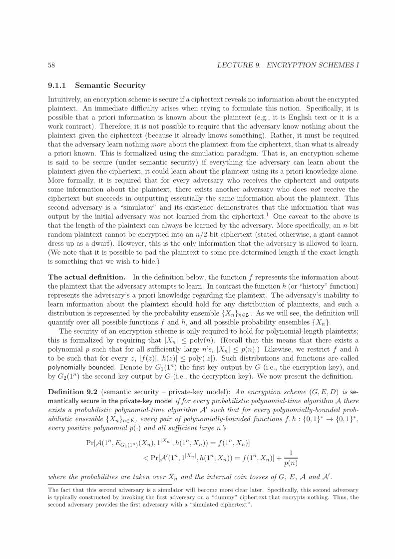
58 LECTURE 9. ENCRYPTION SCHEMES I
9.1.1 Semantic Security
Intuitively, an encryption scheme is secure if a ciphertext reveals no information about the encryptedplaintext. An immediate difficulty arises when trying to formulate this notion. Specifically, it ispossible that a priori information is known about the plaintext (e.g., it is English text or it is awork contract). Therefore, it is not possible to require that the adversary know nothing about theplaintext given the ciphertext (because it already knows something). Rather, it must be requiredthat the adversary learn nothingmore about the plaintext from the ciphertext, than what is alreadya priori known. This is formalized using the simulation paradigm. That is, an encryption schemeis said to be secure (under semantic security) if everything the adversary can learn about theplaintext given the ciphertext, it could learn about the plaintext using its a priori knowledge alone.More formally, it is required that for every adversary who receives the ciphertext and outputssome information about the plaintext, there exists another adversary who does not receive theciphertext but succeeds in outputting essentially the same information about the plaintext. Thissecond adversary is a “simulator” and its existence demonstrates that the information that wasoutput by the initial adversary was not learned from the ciphertext.1 One caveat to the above isthat the length of the plaintext can always be learned by the adversary. More specifically, an n-bitrandom plaintext cannot be encrypted into an n/2-bit ciphertext (stated otherwise, a giant cannotdress up as a dwarf). However, this is the only information that the adversary is allowed to learn.(We note that it is possible to pad the plaintext to some pre-determined length if the exact lengthis something that we wish to hide.)
The actual definition. In the definition below, the function f represents the information aboutthe plaintext that the adversary attempts to learn. In contrast the function h (or “history” function)represents the adversary’s a priori knowledge regarding the plaintext. The adversary’s inability tolearn information about the plaintext should hold for any distribution of plaintexts, and such adistribution is represented by the probability ensemble Xnn∈N. As we will see, the definition willquantify over all possible functions f and h, and all possible probability ensembles Xn.
The security of an encryption scheme is only required to hold for polynomial-length plaintexts;this is formalized by requiring that |Xn| ≤ poly(n). (Recall that this means that there exists apolynomial p such that for all sufficiently large n’s, |Xn| ≤ p(n).) Likewise, we restrict f and hto be such that for every z, |f(z)|, |h(z)| ≤ poly(|z|). Such distributions and functions are calledpolynomially bounded. Denote by G1(1
n) the first key output by G (i.e., the encryption key), andby G2(1
n) the second key output by G (i.e., the decryption key). We now present the definition.
Definition 9.2 (semantic security – private-key model): An encryption scheme (G,E,D) is se-mantically secure in the private-key model if for every probabilistic polynomial-time algorithm A thereexists a probabilistic polynomial-time algorithm A′ such that for every polynomially-bounded prob-abilistic ensemble Xnn∈N, every pair of polynomially-bounded functions f, h : 0, 1∗ → 0, 1∗,every positive polynomial p(·) and all sufficient large n’s
Pr[A(1n, EG1(1n)(Xn), 1|Xn|, h(1n,Xn)) = f(1n,Xn)]
< Pr[A′(1n, 1|Xn|, h(1n,Xn)) = f(1n,Xn)] +1
p(n)
where the probabilities are taken over Xn and the internal coin tosses of G, E, A and A′.
The fact that this second adversary is a simulator will become more clear later. Specifically, this second adversaryis typically constructed by invoking the first adversary on a “dummy” ciphertext that encrypts nothing. Thus, thesecond adversary provides the first adversary with a “simulated ciphertext”.
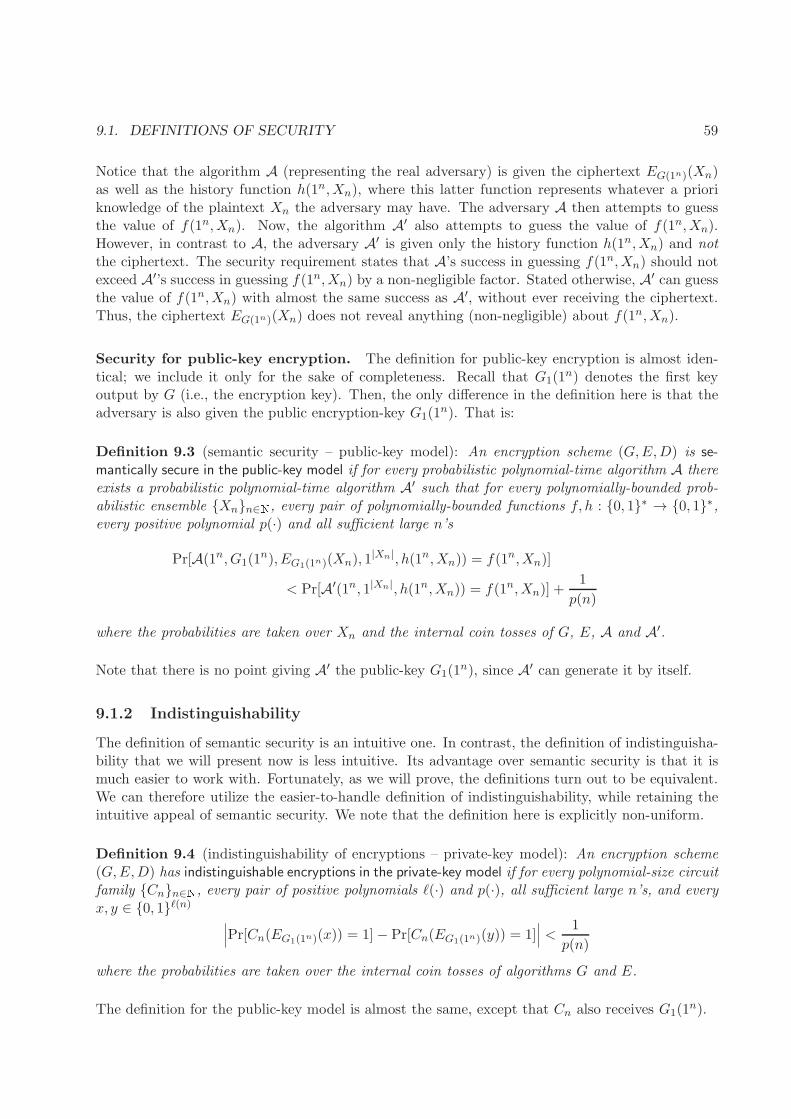
9.1. DEFINITIONS OF SECURITY 59
Notice that the algorithm A (representing the real adversary) is given the ciphertext EG(1n)(Xn)as well as the history function h(1n,Xn), where this latter function represents whatever a prioriknowledge of the plaintext Xn the adversary may have. The adversary A then attempts to guessthe value of f(1n,Xn). Now, the algorithm A′ also attempts to guess the value of f(1n,Xn).However, in contrast to A, the adversary A′ is given only the history function h(1n,Xn) and notthe ciphertext. The security requirement states that A’s success in guessing f(1n,Xn) should notexceed A′’s success in guessing f(1n,Xn) by a non-negligible factor. Stated otherwise, A′ can guessthe value of f(1n,Xn) with almost the same success as A′, without ever receiving the ciphertext.Thus, the ciphertext EG(1n)(Xn) does not reveal anything (non-negligible) about f(1n,Xn).
Security for public-key encryption. The definition for public-key encryption is almost iden-tical; we include it only for the sake of completeness. Recall that G1(1
n) denotes the first keyoutput by G (i.e., the encryption key). Then, the only difference in the definition here is that theadversary is also given the public encryption-key G1(1
n). That is:
Definition 9.3 (semantic security – public-key model): An encryption scheme (G,E,D) is se-mantically secure in the public-key model if for every probabilistic polynomial-time algorithm A thereexists a probabilistic polynomial-time algorithm A′ such that for every polynomially-bounded prob-abilistic ensemble Xnn∈N, every pair of polynomially-bounded functions f, h : 0, 1∗ → 0, 1∗,every positive polynomial p(·) and all sufficient large n’s
Pr[A(1n, G1(1n), EG1(1n)(Xn), 1
|Xn|, h(1n,Xn)) = f(1n,Xn)]
< Pr[A′(1n, 1|Xn|, h(1n,Xn)) = f(1n,Xn)] +1
p(n)
where the probabilities are taken over Xn and the internal coin tosses of G, E, A and A′.
Note that there is no point giving A′ the public-key G1(1n), since A′ can generate it by itself.
9.1.2 Indistinguishability
The definition of semantic security is an intuitive one. In contrast, the definition of indistinguisha-bility that we will present now is less intuitive. Its advantage over semantic security is that it ismuch easier to work with. Fortunately, as we will prove, the definitions turn out to be equivalent.We can therefore utilize the easier-to-handle definition of indistinguishability, while retaining theintuitive appeal of semantic security. We note that the definition here is explicitly non-uniform.
Definition 9.4 (indistinguishability of encryptions – private-key model): An encryption scheme(G,E,D) has indistinguishable encryptions in the private-key model if for every polynomial-size circuitfamily Cnn∈N, every pair of positive polynomials ℓ(·) and p(·), all sufficient large n’s, and everyx, y ∈ 0, 1ℓ(n)
∣
∣
∣Pr[Cn(EG1(1n)(x)) = 1]− Pr[Cn(EG1(1n)(y)) = 1]∣
∣
∣ <1
p(n)
where the probabilities are taken over the internal coin tosses of algorithms G and E.
The definition for the public-key model is almost the same, except that Cn also receives G1(1n).
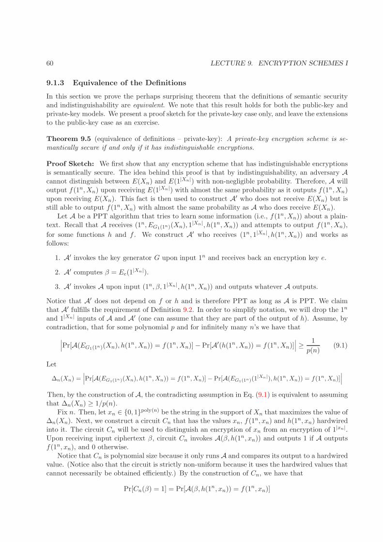
60 LECTURE 9. ENCRYPTION SCHEMES I
9.1.3 Equivalence of the Definitions
In this section we prove the perhaps surprising theorem that the definitions of semantic securityand indistinguishability are equivalent. We note that this result holds for both the public-key andprivate-key models. We present a proof sketch for the private-key case only, and leave the extensionsto the public-key case as an exercise.
Theorem 9.5 (equivalence of definitions – private-key): A private-key encryption scheme is se-mantically secure if and only if it has indistinguishable encryptions.
Proof Sketch: We first show that any encryption scheme that has indistinguishable encryptionsis semantically secure. The idea behind this proof is that by indistinguishability, an adversary Acannot distinguish between E(Xn) and E(1|Xn|) with non-negligible probability. Therefore, A willoutput f(1n,Xn) upon receiving E(1|Xn|) with almost the same probability as it outputs f(1n,Xn)upon receiving E(Xn). This fact is then used to construct A′ who does not receive E(Xn) but isstill able to output f(1n,Xn) with almost the same probability as A who does receive E(Xn).
Let A be a PPT algorithm that tries to learn some information (i.e., f(1n,Xn)) about a plain-text. Recall that A receives (1n, EG1(1n)(Xn), 1
|Xn|, h(1n,Xn)) and attempts to output f(1n,Xn),
for some functions h and f . We construct A′ who receives (1n, 1|Xn|, h(1n,Xn)) and works asfollows:
1. A′ invokes the key generator G upon input 1n and receives back an encryption key e.
2. A′ computes β = Ee(1|Xn|).
3. A′ invokes A upon input (1n, β, 1|Xn|, h(1n,Xn)) and outputs whatever A outputs.
Notice that A′ does not depend on f or h and is therefore PPT as long as A is PPT. We claimthat A′ fulfills the requirement of Definition 9.2. In order to simplify notation, we will drop the 1n
and 1|Xn| inputs of A and A′ (one can assume that they are part of the output of h). Assume, bycontradiction, that for some polynomial p and for infinitely many n’s we have that
∣
∣
∣Pr[A(EG1(1n)(Xn), h(1n,Xn)) = f(1n,Xn)]− Pr[A′(h(1n,Xn)) = f(1n,Xn)]
∣
∣
∣ ≥1
p(n)(9.1)
Let
∆n(Xn) =∣
∣
∣Pr[A(EG1(1n)(Xn), h(1
n, Xn)) = f(1n, Xn)]− Pr[A(EG1(1n)(1|Xn|), h(1n, Xn)) = f(1n, Xn)]
∣
∣
∣
Then, by the construction of A, the contradicting assumption in Eq. (9.1) is equivalent to assumingthat ∆n(Xn) ≥ 1/p(n).
Fix n. Then, let xn ∈ 0, 1poly(n) be the string in the support of Xn that maximizes the value of
∆n(Xn). Next, we construct a circuit Cn that has the values xn, f(1n, xn) and h(1
n, xn) hardwiredinto it. The circuit Cn will be used to distinguish an encryption of xn from an encryption of 1|xn|.Upon receiving input ciphertext β, circuit Cn invokes A(β, h(1n, xn)) and outputs 1 if A outputsf(1n, xn), and 0 otherwise.
Notice that Cn is polynomial size because it only runs A and compares its output to a hardwiredvalue. (Notice also that the circuit is strictly non-uniform because it uses the hardwired values thatcannot necessarily be obtained efficiently.) By the construction of Cn, we have that
Pr[Cn(β) = 1] = Pr[A(β, h(1n, xn)) = f(1n, xn)]
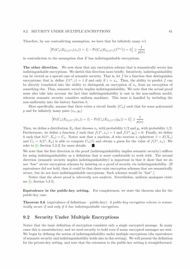
9.2. SECURITY UNDER MULTIPLE ENCRYPTIONS 61
Therefore, by our contradicting assumption, we have that for infinitely many n’s
∣
∣
∣Pr[Cn(EG1(1n)(xn)) = 1]− Pr[Cn(EG1(1n)(1|xn|)) = 1]
∣
∣
∣ ≥1
p(n)
in contradiction to the assumption that E has indistinguishable encryptions.
The other direction. We now show that any encryption scheme that is semantically secure hasindistinguishable encryptions. We sketch this direction more briefly. Intuitively, indistinguishabilitycan be viewed as a special case of semantic security. That is, let f be a function that distinguishesencryptions; that is, define f(1n, z) = 1 if and only if z = xn. Then, the ability to predict f canbe directly translated into the ability to distinguish an encryption of xn from an encryption ofsomething else. Thus, semantic security implies indistinguishability. We note that the actual proofmust also take into account the fact that indistinguishability is cast in the non-uniform model,whereas semantic security considers uniform machines. This issue is handled by including thenon-uniformity into the history function h.
More specifically, assume that there exists a circuit family Cn such that for some polynomialp and for infinitely many pairs (xn, yn)
∣
∣
∣Pr[Cn(EG1(1n)(xn)) = 1]− Pr[Cn(EG1(1n)(yn)) = 1]∣
∣
∣ ≥1
p(n)
Then, we define a distribution Xn that chooses xn with probability 1/2 and yn with probability 1/2.Furthermore, we define a function f such that f(1n, xn) = 1 and f(1n, yn) = 0. Finally, we defineh such that h(1n,Xn) = Cn. Notice now that a machine A who receives a ciphertext β = E(Xn)and Cn = h(1n,Xn) is able to compute Cn(β) and obtain a guess for the value of f(1n, xn). Werefer to [6, Section 5.2.3] for more details.
We note that the first direction in the proof (indistinguishability implies semantic security) sufficesfor using indistinguishability as a definition that is more comfortable to work with. The seconddirection (semantic security implies indistinguishability) is important in that it show that we donot “lose” secure encryption schemes by insisting on a proof of security via indistinguishability. (Ifequivalence did not hold, then it could be that there exist encryption schemes that are semanticallysecure, but do not have indistinguishable encryptions. Such schemes would be “lost”.)
Notice that the above proof is inherently non-uniform. Nevertheless, uniform analogues exist;see [6, Section 5.2.5].
Equivalence in the public-key setting. For completeness, we state the theorem also for thepublic-key case:
Theorem 9.6 (equivalence of definitions – public-key): A public-key encryption scheme is seman-tically secure if and only if it has indistinguishable encryptions.
9.2 Security Under Multiple Encryptions
Notice that the basic definition of encryption considers only a single encrypted message. In manycases this is unsatisfactory, and we need security to hold even if many encrypted messages are sent.We begin by defining the notion of indistinguishability under multiple encryptions (the equivalenceof semantic security and indistinguishability holds also in this setting). We will present the definitionfor the private-key setting, and note that the extension to the public-key setting is straightforward.
62 LECTURE 9. ENCRYPTION SCHEMES I
Definition 9.7 (indistinguishability under multiple encryptions – private key): An encryptionscheme (G,E,D) has indistinguishable encryptions for multiple messages in the private-key model iffor every polynomial-size circuit family, all positive polynomials ℓ(·), t(·) and p(·), all sufficientlylarge n’s, and every x1, . . . , xt(n), y1, . . . , yt(n) ∈ 0, 1
ℓ(n), it holds that∣
∣
∣Pr[Cn(EG1(1n)(x1), . . . , EG1(1n)(xt(n))) = 1]− Pr[Cn(EG1(1n)(y1), . . . , EG1(1n)(yt(n))) = 1]∣
∣
∣ <1
p(n)
We now show that in the public-key setting, indistinguishability for a single message implies in-distinguishability for multiple messages. Unfortunately, the same is not true for the private-keysetting.
9.2.1 Multiple Encryptions in the Public-Key Setting
Theorem 9.8 A public-key encryption scheme has indistinguishable encryptions for multiple mes-sages if and only if it has indistinguishable encryptions for a single message.
Proof: The implication from multiple messages to a single message is trivial. The other direction isproven using a hybrid argument. That is, assume that (G,E,D) has indistinguishable encryptionsfor a single message. Furthermore, assume by contradiction, that there exists a circuit family Cnand polynomials ℓ, t and p such that for infinitely many n’s there exist x1, . . . , xt(n), y1, . . . , yt(n)such that
∣
∣
∣Pr[Cn(G1(1n), EG1(1n)(x1), . . . , EG1(1n)(xt(n))) = 1]
− Pr[Cn(G1(1n), EG1(1n)(y1), . . . , EG1(1n)(yt(n))) = 1]
∣
∣
∣ ≥1
p(n)
We define a hybrid sequence hi = (x1, . . . , xi, yi+1, . . . , yt(n)), and a hybrid distribution H in =
(G1(1n), EG1(1n)(x1), . . . , EG1(1n)(xi), EG1(1n)(yi+1), . . . , EG1(1n)(yt(n))). Then, by the contradicting
assumption we have that
∣
∣
∣Pr[Cn(Ht(n)n ) = 1]− Pr[Cn(H
0n) = 1]
∣
∣
∣ ≥1
p(n)
Using a standard hybrid argument it follows that there exists an i ∈ 0, . . . , t(n)−1 such that
∣
∣
∣Pr[Cn(Hin) = 1]− Pr[Cn(H
i+1n ) = 1]
∣
∣
∣ ≥1
t(n) · p(n)
By hardwiring all of the xj and yk values into a circuit C ′n, we obtain a polynomial-size circuit
family that will distinguish single encryptions. In particular, circuit C ′n receives an encryption β
that is either of xi+1 or yi+1. It then encrypts (by itself) the values x1, . . . , xi and yi+2, . . . , yt(n),
and invokes Cn upon the vector of ciphertexts in which β is placed in the (i+1)th position. If β isan encryption of xi+1, then it follows that C ′
n invoked Cn upon input H i+1n . In contrast, if β is an
encryption of yi+1, then C′n invoked Cn upon input H i
n. It follows that Cn’s ability to distinguishH i
n from H i+1n can be translated into C ′
n’s ability to distinguish xi+1 from yi+1. We stress that thisreduction works only because C ′
n is able to encrypt by itself, since it is given the public-key.

9.2. SECURITY UNDER MULTIPLE ENCRYPTIONS 63
9.2.2 Multiple Encryptions in the Private-Key Setting
Theorem 9.9 Assuming the existence of one-way functions (that are hard to invert for polynomial-size circuits), there exists an encryption scheme that has indistinguishable encryptions for a singlemessage, but does not satisfy Definition 9.7.
The idea behind the proof of this theorem is as follows. Let PRG be a pseudorandom generator(such a PRG exists assuming the existence of one-way functions). Then, define e = G(1n) = Un,Ee(x) = PRG(e)⊕x andDe(y) = PRG(e)⊕y. (We note that in order for this to work, the generatorPRG must stretch e to a length that is any polynomial in n, and not just to a predeterminedpolynomial length.) It is not difficult to prove that Theorem 9.9 holds for this encryption scheme.We leave the details as an exercise.
Conclusion: When constructing encryption schemes in the private-key setting, the security ofthe encryption scheme must be explicitly proven for multiple encryptions.

64 LECTURE 9. ENCRYPTION SCHEMES I
Lecture 10
Encryption Schemes II
In this lecture, we will show how to construct secure encryption schemes in both the private andpublic-key models. We will also extend the definitions of secure encryption to deal with activeadversaries that can carry out chosen-plaintext and chosen-ciphertext attacks.
10.1 Constructing Secure Encryption Schemes
10.1.1 Private-Key Encryption Schemes
In this section, we will show how to construct private-key encryption schemes that are securefor multiple messages. The construction uses pseudorandom functions (recall that these can beconstructed from any one-way function). We will construct a scheme that encrypts plaintexts oflength exactly n (and we assume that the pseudorandom function has input and output of exactlyn bits). In order to obtain a general encryption scheme, where plaintexts can be of any polynomiallength, it is possible to just parse the plaintext into blocks of at most n (with appropriate paddingfor the last block), and encrypt each block separately. This “multiple-encryption” approach isfacilitated by the fact that we prove the security of the basic scheme for multiple encryptions.
Construction 10.1 (private-key encryption – block ciphers): Let F = Fn be an efficiently com-putable function ensemble, and let I and V be the sampling and evaluation functions, respectively,as in Definition 5.1. Then, define (G,E,D) as follows:
• Key generation: G(1n) = (k, k), where k ← I(1n).
• Encryption of x ∈ 0, 1n using key k: Ek(x) = (r, V (k, r)⊕ x) where r ∈R 0, 1n.
• Decryption of (r, y) using key k: Dk(r, y) = V (k, r)⊕ y.
We proceed to prove the security of the above construction:
Theorem 10.2 Assume that F is a family of functions that is pseudorandom to polynomial-sizecircuits. Then, (G,E,D) described in Construction 10.1 is a private-key encryption scheme withindistinguishable encryptions for multiple messages.
* Lecture notes for a graduate course in the theory of cryptography. Yehuda Lindell, Bar-Ilan University, Israel, 2005.
65
66 LECTURE 10. ENCRYPTION SCHEMES II
Proof Sketch: Assume first that F is a truly random function family. Let x1, . . . , xt(n) andy1, . . . , yt(n) be two vectors of plaintexts. Now, assume that the r values appearing in all theciphertexts are distinct. (That is, let ci = (ri, fi). Then, assume that for all i 6= j it holds thatri 6= rj .) Then, it follows that Ek(xi) is distributed identically to Ek(yi). This is due to thefact that F is truly random and so if all ri’s are distinct, then all F (ri)’s are independently anduniformly distributed in 0, 1n. The probability of distinguishing a vector of encryptions of thex values from a vector of encryptions of the y values therefore equals at most t(n)2 · 2−n (whichupper bounds the probability that at least one pair i and j are such that ri = rj).
Next, we replace the random function by a pseudorandom one and claim that if the scheme nowbecomes “distinguishable”, then this yields a distinguisher for the pseudorandom function.
We note the use of random coin tosses in the encryption process. We will not elaborate on this, asit was discussed at length in the course “Introduction to Cryptography” (89-656).
10.1.2 Public-Key Encryption Schemes
In this section, we will show how to construct public-key encryption schemes. In contrast to private-key encryption, our constructions here require the use of trapdoor one-way permutations (ratherthan one-way functions). We will first show how to encrypt a single bit; encryption of arbitrary-length messages can be obtained by encrypting each bit separately. (Recall that in the public-keysetting, the extension from the single-message to the multiple-message setting is automatic.)
Encrypting a single bit. Let (I, S, F, F−1) be a collection of trapdoor one-way permutations,as in Definition 2.3 (we denote the domain sampling algorithm by S so as not to confuse it withthe decryption algorithm D). The idea behind this construction is to encrypt a bit σ by outputting(f(Un), b(Un)⊕ σ), where f is the sampled permutation and b is a hard-core predicate of f . Recallthat this output is pseudorandom (as proven earlier in the course), and so intuitively σ will be“hidden” as required. Furthermore, notice that decryption can be carried out using the trapdoor.In particular, given (f(r), τ) where τ = b(r)⊕ σ, it is possible to use the trapdoor to obtain r andthen compute b(r) and σ = τ ⊕ b(r).
Construction 10.3 (public-key encryption): Let (I, S, F, F−1) be a collection of trapdoor permu-tations and let B be a predicate. Then, define (G,E,D) as follows:
• Key generation: G(1n) = (i, t), where i = I1(1n) is the first element of the output of I(1n)
and t is the second element of the output of I(1n), or the “trapdoor”.
• Encryption of σ ∈ 0, 1 using key i: Sample a random element x according to S(i) andcompute y = F (i, x). Output (y, τ) where τ = B(i, x)⊕ σ.
• Decryption of (y, τ) using key (i, t): Compute x = F−1(t, y) and output σ = B(i, x)⊕ τ .
We now prove the security of the above construction:
Theorem 10.4 Assume that (I, S, F, F−1) is a collection of trapdoor one-way permutations andthat B is a hard-core predicate of (I, S, F ), where hardness holds for non-uniform adversaries. Then,(G,E,D) described in Construction 10.3 is a public-key encryption scheme with indistinguishableencryptions.
10.1. CONSTRUCTING SECURE ENCRYPTION SCHEMES 67
Proof Sketch: The fact that (G,E,D) constitutes an encryption scheme is immediate. Regardingits security, it suffices to show that for i← I(1n), it is hard to distinguish between the distributionsi, Ei(0) ≡ i, (F (i, x), B(i, x)) and i, Ei(1) ≡ i, (F (i, x), B(i, x)), where i ← I(1n) andx ← S(i). In the proof of Theorem 4.7 we proved an almost identical fact. (The only differencehere is that we are using a collection of permutations, instead of a single one-way permutation.However, this makes no difference to the specific fact being referred to.) We thus conclude that theconstructed encryption scheme is secure.
The encryption scheme of Construction 10.3 is very inefficient. In particular, for every bit of theplaintext, the ciphertext contains n + 1 bits. Thus, the size of the ciphertext is n times the sizeof the plaintext. We will now present a construction that is more efficient with respect to thebandwidth. (Unfortunately, it still requires an application of F (i, ·) for every bit of the plaintextand so is still computationally very heavy.)
Construction 10.5 (public-key encryption – efficient construction): Let (I, S, F, F−1) be a collec-tion of trapdoor permutations and let B be a predicate. Then, define (G,E,D) as follows:
• Key generation: G(1n) = (i, t), where i = I1(1n) is the first element of the output of I(1n)
and t is the second element of the output of I(1n), or the “trapdoor”.
• Encryption of σ ∈ 0, 1ℓ using key i: Let σ = σ0 · · · σℓ−1 where for every j, σj ∈ 0, 1.Sample a random element x according to S(i) and set x0 = x. Then, for j = 1, . . . , ℓ, set xj =F (i, xj−1). Finally, for j = 0, . . . , ℓ− 1, set τj = B(i, xj)⊕ σj and output (xℓ, τ0, . . . , τℓ−1).
• Decryption of (xℓ, τ0, . . . , τℓ−1) using key (i, t): Compute x0 = F−ℓ(t, xℓ) and then reconstructthe series B(i, x0), . . . , B(i, xℓ−1) and output σ = σ0 · · · σℓ−1 by computing σj = τj ⊕B(i, xj)for every j.
We prove the security of the above construction:
Theorem 10.6 Assume that (I, S, F, F−1) is a collection of trapdoor one-way permutations andthat B is a hard-core predicate of (I, S, F ), where hardness holds for non-uniform adversaries. Then,(G,E,D) described in Construction 10.5 is a public-key encryption scheme with indistinguishableencryptions.
Proof Sketch: The fact that (G,E,D) constitutes an encryption scheme is straightforward.Denote by Gℓ
i(x0) the series B(i, x0), . . . , B(i, xℓ−1). Then, in order to prove security, we need toprove that for every polynomial ℓ and every σ, σ′ ∈ 0, 1ℓ(n), it holds that
i, F ℓ(i, x0), Gℓi(x0)⊕ σ
n∈N c≡
i, F ℓ(i, x0), Gℓi(x0)⊕ σ
′
n∈N (10.1)
where i ← I(1n) and x0 ← S(i), and where indistinguishability holds with respect to polynomial-size circuits. We show that
i, F ℓ(i, x0), Gℓi(x0)
n∈N c≡
i, F ℓ(i, x0), Uℓ
n∈N (10.2)
which clearly implies Eq. (10.1). (We note that the entire distribution is not necessarily pseudo-random because F ℓ(i, x0) may not be pseudorandom. This is due to the fact that the domain of Fis not necessarily 0, 1n.) In order to prove Eq. (10.2) we rely on the fact that
i, F (i, x), B(i, x)n∈N c≡ i, F (i, x), U1n∈N (10.3)
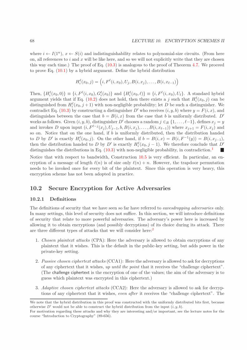
68 LECTURE 10. ENCRYPTION SCHEMES II
where i← I(1n), x← S(i) and indistinguishability relates to polynomial-size circuits. (From hereon, all references to i and x will be like here, and so we will not explicitly write that they are chosenthis way each time.) The proof of Eq. (10.3) is analogous to the proof of Theorem 4.7. We proceedto prove Eq. (10.1) by a hybrid argument. Define the hybrid distribution
Hℓi (x0, j) =
(
i, F ℓ(i, x0), Uj , B(i, xj), . . . , B(i, xℓ−1))
Then, Hℓi (x0, 0) ≡ i, F
ℓ(i, x0), Gℓi(x0) and H
ℓi (x0, ℓ) ≡ i, F
ℓ(i, x0), Uℓ. A standard hybridargument yields that if Eq. (10.2) does not hold, then there exists a j such that Hℓ
i (x0, j) can bedistinguished from Hℓ
i (x0, j +1) with non-negligible probability; let D be such a distinguisher. Wecontradict Eq. (10.3) by constructing a distinguisher D′ who receives (i, y, b) where y = F (i, x), anddistinguishes between the case that b = B(i, x) from the case that b is uniformly distributed. D′
works as follows. Given (i, y, b), distinguisherD′ chooses a random j ∈R 1, . . . , ℓ−1, defines xj = yand invokes D upon input (i, F ℓ−j(xj), Uj−1, b, B(i, xj), . . . , B(i, xℓ−1)) where xj+1 = F (i, xj) andso on. Notice that on the one hand, if b is uniformly distributed, then the distribution handedto D by D′ is exactly Hℓ
i (x0, j). On the other hand, if b = B(i, x) = B(i, F−1(y)) = B(i, xj−1),then the distribution handed to D by D′ is exactly Hℓ
i (x0, j − 1). We therefore conclude that D′
distinguishes the distributions in Eq. (10.3) with non-negligible probability, in contradiction.1
Notice that with respect to bandwidth, Construction 10.5 is very efficient. In particular, an en-cryption of a message of length ℓ(n) is of size only ℓ(n) + n. However, the trapdoor permutationneeds to be invoked once for every bit of the plaintext. Since this operation is very heavy, thisencryption scheme has not been adopted in practice.
10.2 Secure Encryption for Active Adversaries
10.2.1 Definitions
The definitions of security that we have seen so far have referred to eavesdropping adversaries only.In many settings, this level of security does not suffice. In this section, we will introduce definitionsof security that relate to more powerful adversaries. The adversary’s power here is increased byallowing it to obtain encryptions (and possibly decryptions) of its choice during its attack. Thereare three different types of attacks that we will consider here:2
1. Chosen plaintext attacks (CPA): Here the adversary is allowed to obtain encryptions of anyplaintext that it wishes. This is the default in the public-key setting, but adds power in theprivate-key setting.
2. Passive chosen ciphertext attacks (CCA1): Here the adversary is allowed to ask for decryptionsof any ciphertext that it wishes, up until the point that it receives the “challenge ciphertext”.(The challenge ciphertext is the encryption of one of the values; the aim of the adversary is toguess which plaintext was encrypted in this ciphertext.)
3. Adaptive chosen ciphertext attacks (CCA2): Here the adversary is allowed to ask for decryp-tions of any ciphertext that it wishes, even after it receives the “challenge ciphertext”. The
We note that the hybrid distribution in this proof was constructed with the uniformly distributed bits first, becauseotherwise D′ would not be able to construct the hybrid distribution from the input (i, y, b).For motivation regarding these attacks and why they are interesting and/or important, see the lecture notes for thecourse “Introduction to Cryptography” (89-656).
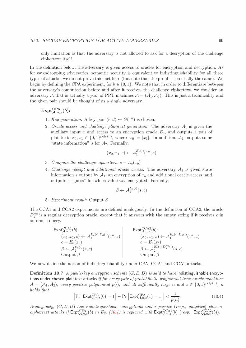
10.2. SECURE ENCRYPTION FOR ACTIVE ADVERSARIES 69
only limitation is that the adversary is not allowed to ask for a decryption of the challengeciphertext itself.
In the definition below, the adversary is given access to oracles for encryption and decryption. Asfor eavesdropping adversaries, semantic security is equivalent to indistinguishability for all threetypes of attacks; we do not prove this fact here (but note that the proof is essentially the same). Webegin by defining the CPA experiment, for b ∈ 0, 1. We note that in order to differentiate betweenthe adversary’s computation before and after it receives the challenge ciphertext, we consider anadversary A that is actually a pair of PPT machines A = (A1,A2). This is just a technicality andthe given pair should be thought of as a single adversary.
ExptCPA
A,n,z(b):
1. Key generation: A key-pair (e, d)← G(1n) is chosen.
2. Oracle access and challenge plaintext generation: The adversary A1 is given theauxiliary input z and access to an encryption oracle Ee, and outputs a pair ofplaintexts x0, x1 ∈ 0, 1
poly(n), where |x0| = |x1|. In addition, A1 outputs some“state information” s for A2. Formally,
(x0, x1, s)← AEe(·)1 (1n, z)
3. Compute the challenge ciphertext: c = Ee(xb)
4. Challenge receipt and additional oracle access: The adversary A2 is given stateinformation s output by A1, an encryption of xb and additional oracle access, andoutputs a “guess” for which value was encrypted. Formally,
β ← AEe(·)2 (s, c)
5. Experiment result: Output β
The CCA1 and CCA2 experiments are defined analogously. In the definition of CCA2, the oracleD¬c
d is a regular decryption oracle, except that it answers with the empty string if it receives c inan oracle query.
ExptCCA1A,n,z (b): ExptCCA2
A,n,z (b):
(x0, x1, s)← AEe(·),Dd(·)1 (1n, z) (x0, x1, s)← A
Ee(·),Dd(·)1 (1n, z)
c = Ee(xb) c = Ee(xb)
β ← AEe(·)2 (s, c) β ← A
Ee(·),D¬cd
(·)2 (s, c)
Output β Output β
We now define the notion of indistinguishability under CPA, CCA1 and CCA2 attacks.
Definition 10.7 A public-key encryption scheme (G,E,D) is said to have indistinguishable encryp-tions under chosen plaintext attacks if for every pair of probabilistic polynomial-time oracle machinesA = (A1,A2), every positive polynomial p(·), and all sufficiently large n and z ∈ 0, 1poly(n), itholds that
∣
∣
∣Pr[
ExptCPAA,n,z(0) = 1
]
− Pr[
ExptCPAA,n,z(1) = 1
]∣
∣
∣ <1
p(n)(10.4)
Analogously, (G,E,D) has indistinguishable encryptions under passive (resp., adaptive) chosen-ciphertext attacks if ExptCPA
A,n,z(b) in Eq. (10.4) is replaced with ExptCCA1A,n,z (b) (resp., Expt
CCA2A,n,z (b)).

70 LECTURE 10. ENCRYPTION SCHEMES II
10.2.2 Constructions
We first note that the public-key encryption schemes described in Constructions 10.3 and 10.5 aresecure under chosen-plaintext attacks. Intuitively, this follows from the fact that in the public-keysetting, the adversary is anyway given the encryption key (and so can encrypt by itself). Technically,the definitions are actually not equivalent because the challenge plaintexts in a chosen-plaintextattack may depend on the public-key, which is not the case in the eavesdropping case. Nevertheless,it is not hard to see that the same proof goes through also for the case of CPA-attacks.
Next, we note that the private-key encryption scheme described in Construction 10.1 is alsosecure under chosen-plaintext attacks. This does not follow from the definitions, because theadversary’s power in the eavesdropping setting is strictly weaker than in a CPA attack (even if itreceives multiple encryptions). Nevertheless, this is also easily demonstrated and we leave it as anexercise.
CCA2-security in the private-key setting. In the course “Introduction to Cryptography”,we stated that CCA2-secure private-key encryption can be obtained by first encrypting the messageusing a private-key encryption scheme that is CPA-secure, and then applying a message authenti-cation code (MAC) to the result. We leave the formal definition and proof of this construction asan exercise.
CCA1 and CCA2 security in the public-key setting. Unfortunately, constructions for thesesettings are far more complicated than in the private-key setting. We leave these (specifically CCA2)as a reading assignment. This also involves learning non-interactive zero-knowledge which we willdescribe on a high-level in class. The reading material will be placed on the course website. Startwith the material on non-interactive zero-knowledge, taken from the fragments of a book preceding[5], and focus on understanding the model and definitions. (It is also important to understandthe constructions, but the definitions are crucial for the next stage.) Then, read the paper thatpresents a construction of a public-key encryption scheme that is CCA2-secure (read the appendixas well). Focus on the main ideas (and not technicalities that you may not be familiar with).

Lecture 11
Digital Signatures I
In this lecture, we will present definitions of digital signatures and show how to construct full-fledged digital signatures from length-restricted ones. As regarding encryption schemes, we willnot present motivation to the notion of digital signatures, and will not discuss applications. Thismaterial can be found in the lecture notes for the course “Introduction to Cryptography” (89-656).
11.1 Defining Security for Signature Schemes
We begin by presenting the syntax of digital signature schemes.
Definition 11.1 A digital signature scheme consists of a triple of probabilistic polynomial-timealgorithms (G,S, V ) satisfying the following conditions:
1. On input 1n, the key-generator algorithm G outputs a pair of keys (s, v).
2. For every pair (s, v) in the range of G(1n) and for every α ∈ 0, 1∗, the signing and verificationalgorithms S and V satisfy
Pr[V (v, α, S(s, α)) = 1] = 1
where the probability is taken over the internal coin tosses of algorithms S and V .
The integer n serves as the security parameter of the scheme. The key s is called the signing key,the key v is called the verification key, and a string σ = S(s, α) is called a digital signature. Forshorthand, we will often denote Ss(α) = S(s, α) and Vv(α, σ) = V (v, α, σ).
As with encryption, the requirement that verification always succeeds can be relaxed to allow failurewith negligible probability.
Defining security for signature schemes. The security requirement for a signature schemestates that a PPT adversary A should succeed in generating a valid “forgery” with at most negligibleprobability. In order to model the fact that the adversary A may see signatures generated by thereal signer, A is given access to a signing oracle. Such an attack is called a chosen message attack(because A chooses the messages to be signed). In addition, the adversary A is said to succeed ingenerating an existential forgery if it generates a pair (α, σ) where V (v, α, σ) = 1 and where α wasnot queried to the signing oracle. (The forgery is “existential” because there are no constraints onthe message α.) More formally, the following experiment is defined:
* Lecture notes for a graduate course in the theory of cryptography. Yehuda Lindell, Bar-Ilan University, Israel, 2005.
71
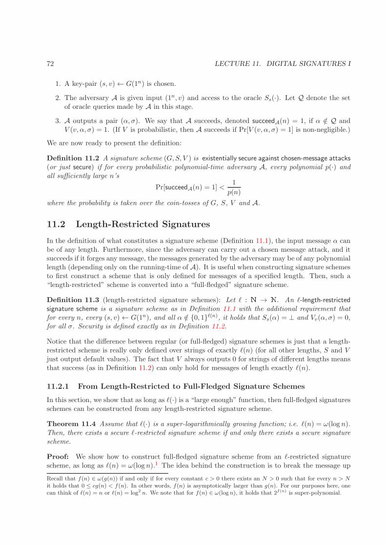
72 LECTURE 11. DIGITAL SIGNATURES I
1. A key-pair (s, v)← G(1n) is chosen.
2. The adversary A is given input (1n, v) and access to the oracle Ss(·). Let Q denote the setof oracle queries made by A in this stage.
3. A outputs a pair (α, σ). We say that A succeeds, denoted succeedA(n) = 1, if α /∈ Q andV (v, α, σ) = 1. (If V is probabilistic, then A succeeds if Pr[V (v, α, σ) = 1] is non-negligible.)
We are now ready to present the definition:
Definition 11.2 A signature scheme (G,S, V ) is existentially secure against chosen-message attacks(or just secure) if for every probabilistic polynomial-time adversary A, every polynomial p(·) andall sufficiently large n’s
Pr[succeedA(n) = 1] <1
p(n)
where the probability is taken over the coin-tosses of G, S, V and A.
11.2 Length-Restricted Signatures
In the definition of what constitutes a signature scheme (Definition 11.1), the input message α canbe of any length. Furthermore, since the adversary can carry out a chosen message attack, and itsucceeds if it forges any message, the messages generated by the adversary may be of any polynomiallength (depending only on the running-time of A). It is useful when constructing signature schemesto first construct a scheme that is only defined for messages of a specified length. Then, such a“length-restricted” scheme is converted into a “full-fledged” signature scheme.
Definition 11.3 (length-restricted signature schemes): Let ℓ : N → N. An ℓ-length-restrictedsignature scheme is a signature scheme as in Definition 11.1 with the additional requirement thatfor every n, every (s, v)← G(1n), and all α /∈ 0, 1ℓ(n), it holds that Ss(α) = ⊥ and Vv(α, σ) = 0,for all σ. Security is defined exactly as in Definition 11.2.
Notice that the difference between regular (or full-fledged) signature schemes is just that a length-restricted scheme is really only defined over strings of exactly ℓ(n) (for all other lengths, S and Vjust output default values). The fact that V always outputs 0 for strings of different lengths meansthat success (as in Definition 11.2) can only hold for messages of length exactly ℓ(n).
11.2.1 From Length-Restricted to Full-Fledged Signature Schemes
In this section, we show that as long as ℓ(·) is a “large enough” function, then full-fledged signaturesschemes can be constructed from any length-restricted signature scheme.
Theorem 11.4 Assume that ℓ(·) is a super-logarithmically growing function; i.e. ℓ(n) = ω(log n).Then, there exists a secure ℓ-restricted signature scheme if and only there exists a secure signaturescheme.
Proof: We show how to construct full-fledged signature scheme from an ℓ-restricted signaturescheme, as long as ℓ(n) = ω(log n).1 The idea behind the construction is to break the message up
Recall that f(n) ∈ ω(g(n)) if and only if for every constant c > 0 there exists an N > 0 such that for every n > Nit holds that 0 ≤ cg(n) < f(n). In other words, f(n) is asymptotically larger than g(n). For our purposes here, onecan think of ℓ(n) = n or ℓ(n) = log2 n. We note that for f(n) ∈ ω(logn), it holds that 2f(n) is super-polynomial.
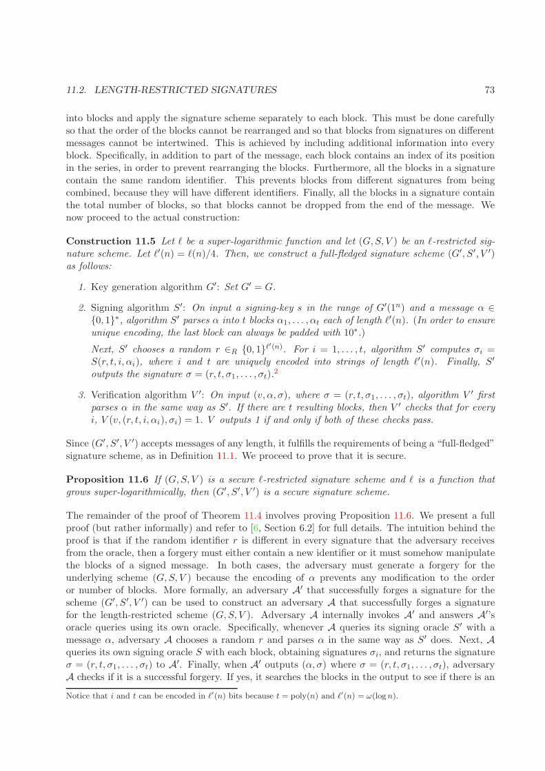
11.2. LENGTH-RESTRICTED SIGNATURES 73
into blocks and apply the signature scheme separately to each block. This must be done carefullyso that the order of the blocks cannot be rearranged and so that blocks from signatures on differentmessages cannot be intertwined. This is achieved by including additional information into everyblock. Specifically, in addition to part of the message, each block contains an index of its positionin the series, in order to prevent rearranging the blocks. Furthermore, all the blocks in a signaturecontain the same random identifier. This prevents blocks from different signatures from beingcombined, because they will have different identifiers. Finally, all the blocks in a signature containthe total number of blocks, so that blocks cannot be dropped from the end of the message. Wenow proceed to the actual construction:
Construction 11.5 Let ℓ be a super-logarithmic function and let (G,S, V ) be an ℓ-restricted sig-nature scheme. Let ℓ′(n) = ℓ(n)/4. Then, we construct a full-fledged signature scheme (G′, S′, V ′)as follows:
1. Key generation algorithm G′: Set G′ = G.
2. Signing algorithm S′: On input a signing-key s in the range of G′(1n) and a message α ∈0, 1∗, algorithm S′ parses α into t blocks α1, . . . , αt each of length ℓ′(n). (In order to ensureunique encoding, the last block can always be padded with 10∗.)
Next, S′ chooses a random r ∈R 0, 1ℓ′(n). For i = 1, . . . , t, algorithm S′ computes σi =
S(r, t, i, αi), where i and t are uniquely encoded into strings of length ℓ′(n). Finally, S′
outputs the signature σ = (r, t, σ1, . . . , σt).2
3. Verification algorithm V ′: On input (v, α, σ), where σ = (r, t, σ1, . . . , σt), algorithm V ′ firstparses α in the same way as S′. If there are t resulting blocks, then V ′ checks that for everyi, V (v, (r, t, i, αi), σi) = 1. V outputs 1 if and only if both of these checks pass.
Since (G′, S′, V ′) accepts messages of any length, it fulfills the requirements of being a “full-fledged”signature scheme, as in Definition 11.1. We proceed to prove that it is secure.
Proposition 11.6 If (G,S, V ) is a secure ℓ-restricted signature scheme and ℓ is a function thatgrows super-logarithmically, then (G′, S′, V ′) is a secure signature scheme.
The remainder of the proof of Theorem 11.4 involves proving Proposition 11.6. We present a fullproof (but rather informally) and refer to [6, Section 6.2] for full details. The intuition behind theproof is that if the random identifier r is different in every signature that the adversary receivesfrom the oracle, then a forgery must either contain a new identifier or it must somehow manipulatethe blocks of a signed message. In both cases, the adversary must generate a forgery for theunderlying scheme (G,S, V ) because the encoding of α prevents any modification to the orderor number of blocks. More formally, an adversary A′ that successfully forges a signature for thescheme (G′, S′, V ′) can be used to construct an adversary A that successfully forges a signaturefor the length-restricted scheme (G,S, V ). Adversary A internally invokes A′ and answers A′’soracle queries using its own oracle. Specifically, whenever A queries its signing oracle S′ with amessage α, adversary A chooses a random r and parses α in the same way as S′ does. Next, Aqueries its own signing oracle S with each block, obtaining signatures σi, and returns the signatureσ = (r, t, σ1, . . . , σt) to A′. Finally, when A′ outputs (α, σ) where σ = (r, t, σ1, . . . , σt), adversaryA checks if it is a successful forgery. If yes, it searches the blocks in the output to see if there is an
Notice that i and t can be encoded in ℓ′(n) bits because t = poly(n) and ℓ′(n) = ω(logn).
74 LECTURE 11. DIGITAL SIGNATURES I
i such that A did not query (αi, i, t, r) with its oracle, where αi is constructed in the usual way. Ifyes, it outputs ((r, t, i, αi), σi) and halts. If not, it output fail and halts.
It remains to show that if A′ generated a successful forgery, then with overwhelming probability,so did A. Let (α, σ) where σ = (r, t, σ1, . . . , σt) be a successful forgery for A′ in the “game” withA. We have the following cases:
1. The identifier in the forged signature of A′ is different from all identifiers generated by A: Inthis case, it is clear that every block of the signature constitutes a successful forgery for A.
2. The identifier in the forged signature equals the identifier in exactly one of the signaturessupplied to A′: Let σ′ be the signature received by A′ with the same identifier as in the forgery,and let α′ be the corresponding signed message. If the output of A′ is a successful forgery,then the message α must be different to all previously signed messages, and in particularmust be different to α′. Let t and t′ be the number of blocks in the parsing of α and α′,respectively. There are two subcases here:
(a) Case 1 – t = t′: In this case, the α-content of one of the blocks must be different (i.e., forsome i it must be that (αi, i) 6= (α′
i, i)). This block constitutes a successful forgery forA. In order to see this, note that A queried its oracle with (α′
i, i, t, r), and furthermorethat there was only a single query of the form (∗, i, ∗, r). (This is due to the fact that rwas only used once.) Since (α′
i, i) 6= (αi, i), we have that this block constitutes a forgeryfor A.
(b) Case 2 – t 6= t′: In this case, each block constitutes a successful forgery for A. Thisfollows from the following two facts. First, in this case, the only signature generated byA for A′ that has the identifier r is the signature on the message α′. Second, t′ 6= t.Combining these facts we have that A never queried its oracle with a message of theform (r, t, ∗, ∗). However all of the blocks in A′’s forgery are of this form. They thereforeall constitute a successful forgery for A.
3. The identifier in the forged signature equals the identifier in at least two signatures suppliedto A′: We rule out this case by showing the two signatures (generated legally) have the thesame identifier with at most negligible probability. Now, the length of a random identifieris ℓ′(n) = ℓ(n)/4 and ℓ(n) is super-logarithmic. Therefore 2−ℓ′(n) is a negligible function.Now, for m signatures, the probability that at least two signatures have the same identifier
is
(
m2
)
· 2−ℓ′(n) = poly(n) · µ(n) which is negligible.
This completes the proof.
Notice that Theorem 11.4 is very strong in that it requires no additional assumptions for con-structing a full-fledge signature scheme from an ℓ-restricted one. It is therefore useful for provingfeasibility results.
11.2.2 Collision-Resistant Hash Functions and Extending Signatures
In this section, we present an alternative way of constructing full-fledged signature schemes fromlength-restricted ones. Specifically, the message is first hashed with a collision-resistant hash func-tion, and the result is then signed. This methodology requires additional complexity assumptions(namely, the existence of collision-resistant hash functions), but is more efficient, at least withrespect to bandwidth. Another advantage of the hash-based extension is that it is also applicable
11.2. LENGTH-RESTRICTED SIGNATURES 75
to one-time signatures schemes (these are signature schemes that can be used to sign only a singlemessage). We will study one-time signatures schemes in Section 12.2.
We begin by defining the notion of collision-resistant hash functions. (Once again, we referstudents to the lecture notes for the course “Introduction to Cryptography” (89-656) for backgroundmaterial and motivation.)
Definition 11.7 (collision-resistant hash functions): Let ℓ : N → N. A collection of functionsH = hr : 0, 1∗ → 0, 1ℓ(|r|) is called a family of collision-resistant hash functions if there existsa probabilistic polynomial-time sampling algorithm I such that the following holds:
1. There exists a polynomial-time algorithm that, given r and x, returns hr(x).
2. For every probabilistic polynomial-time algorithm A, every positive polynomial p(·) and allsufficiently large n’s
Pr[
A(I(1n), 1n) = (x, x′) & x 6= x′ & hI(1n)(x) = hI(1n)(x′)]
<1
p(n)
where the probability is taken over the coin tosses of I and A.3
The function ℓ(·) is called the range-length of H.
We note that any family of collision-resistant hash functions is a collection of one-way functions.We leave the proof of this as an exercise.
The hash-and-sign construction for signatures is simple: In order to sign on an arbitrary-lengthmessage α, first compute hr(α) in order to obtain a message of length ℓ and then apply an ℓ-restricted signature scheme. In order to simplify the description, we assume that |r| = n and thusthe output of the hash function is exactly ℓ(n) for all r ← I(1n). A more formal description of theconstruction is as follows:
Construction 11.8 Let (G,S, V ) be an ℓ-restricted signature scheme and let H be a family ofhash functions with range-length ℓ. Then, define (G′, S′, V ′) as follows:
1. Key generation G′: Upon input 1n, compute (s, v) ← G(1n) and r ← I(1n). Let s′ = (s, r)and v′ = (v, r); output (s′, v′).
2. Signature algorithm S′: Given key (s, r) and message α, output σ = Ss(hr(α)).
3. Verification algorithm V ′: Given key (v, r), message α and signature σ, output Vv(hr(α), σ).
We have the following proposition:
Proposition 11.9 Let ℓ : N→ N. Assume that (G,S, V ) is a secure ℓ-restricted signature schemeand that H is a family of collision-resistant hash functions with range-length ℓ. Then, (G′, S′, V ′)from Construction 11.8 is a secure signature scheme.
Note that the “and” in the probability is not between two random variables, because the right-hand side has noprobability. Rather it should be interpreted as “such that”.

76 LECTURE 11. DIGITAL SIGNATURES I
Proof Sketch: We present only a very brief overview of the proof. Given an adversary A′ whofinds a collision in (G′, S′, V ′) we construct A who either finds a collision in H or computes aforgery in (G,S, V ). Adversary A invokes A′ and upon receiving an oracle query α, it queries itsown oracle with hr(α). Assume that A′ outputs a successful forgery (α′, σ′). Then there are twocases:
1. There exists a message α that was previously queried such that hr(α) = hr(α′): In this case,
A′ found a collision in H.
2. There does not exist such a message α: In this case, A′ obtained a forgery in (G,S, V ).
The full proof works by constructing two adversaries: one corresponding to each case. Then, if A′
succeeds in generating a forgery with non-negligible probability, one of the two adversaries mustalso succeed with non-negligible probability.
11.2.3 Constructing Collision-Resistant Hash Functions
Unfortunately, due to lack of time, we do not have time to show how to construct collision-resistanthash functions (with proven security). The construction is not complicated and is well-worthreading. This material can be found in [6, Section 6.2.3]; it refers to claw-free permutations thatare presented in [5, Section 2.4.5]. We note that claw-free permutations, and thus collision-resistanthash functions, can be constructed assuming that the factoring or discrete log problems are hard.
Lecture 12
Digital Signatures II
In this lecture, we will show how to construct secure digital signatures.
12.1 Minimal Assumptions for Digital Signatures
Until now, we have seen that “private-key cryptography” can be obtained assuming only the ex-istence of one-way functions. This is true of primitives, such as pseudorandom generators andfunctions, as well as applications such as private-key encryption and message authentication codes.In contrast, it is not known how to construct public-key encryption from one-way functions (andblack-box constructions of public-key encryption from one-way functions have been proven to notexist). Rather, known (general) constructions of public-key encryption schemes require the exis-tence of trapdoor one-way permutations. Intuitively, this is due to the fact that decryption involvesinverting something, and so some trapdoor information is needed.
In contrast to encryption, the “public-key” problem of digital signatures can be solved relyingonly on the existence of one-way functions. That is, we have the following theorem:
Theorem 12.1 Secure digital signature schemes exists if and only if one-way functions exist.
We will not prove the above result, but will rather present a simpler construction that relies oncollision-resistant hash functions. Due to lack of time will also only present a memory-dependentsignature scheme, meaning that the signing algorithm must record the history of all previoussignatures. This actually suffices for many applications, although it is clearly undesirable. Wewill also outline the construction of a full memoryless signature scheme, and refer to [6, Section6.4] for a full description.
12.2 Secure One-Time Signature Schemes
We begin by constructing signature schemes that are secure as long as only a single message issigned. These are of independent interest, but also form the basis of our general construction. Weomit a formal definition of security for one-time signature schemes, but note that it suffices to limitthe adversary to a single oracle query, and everything else remains the same.
* Lecture notes for a graduate course in the theory of cryptography. Yehuda Lindell, Bar-Ilan University, Israel, 2005.
77
78 LECTURE 12. DIGITAL SIGNATURES II
12.2.1 Length-Restricted One-Time Signature Schemes
Construction 12.2 (an ℓ-restricted one-time signature scheme): Let ℓ : N → N be polynomi-ally bounded and polynomial-time computable, and let f : 0, 1∗ → 0, 1∗ be a polynomial-timecomputable function. The scheme (G,S, V ) is defined as follows:
1. Key generation G: On input 1n, G uniformly chooses strings s01, s11, . . . , s
0ℓ(n), s
1ℓ(n) ∈R 0, 1
n,
and computes vbi = f(sbi), for every 1 ≤ i ≤ ℓ(n) and b ∈ 0, 1. G outputs the keys (s, v)where s = ((s01, s
11), . . . , (s
0ℓ(n), s
1ℓ(n))) and v = ((v01 , v
11), . . . , (v
0ℓ(n), v
1ℓ(n))).
2. Signing algorithm S: Upon input s and α ∈ 0, 1ℓ(n), algorithm S outputs σ = (sα11 , . . . , s
αℓ(n)
ℓ(n) )where α = α1 · · ·αℓ(n).
3. Verification algorithm V : Upon input v, α ∈ 0, 1ℓ(n) and σ, check that for every i =1, . . . , ℓ(n) it holds that f(sαi
i ) = vαi
i .
Proposition 12.3 If f is a one-way function, then Construction 12.2 constitutes a secure ℓ-restricted one-time signature scheme.
Proof Sketch: The intuition behind the security of Construction 12.2 is that a forgery can onlybe obtained by inverting the one-way function f . Specifically, recall that the adversary can onlysee a single signature before it outputs its forgery; let α be this message and let α′ be the messageof the forgery. Now, if the adversary succeeds, it must be that α′ 6= α and so for some i it holdsthat α′
i 6= αi. The signature that the adversary received for α contained the pre-image sαi
i and not
the pre-image s1−αi
i = sα′
i
i . Thus, if the adversary presented a valid forgery for α′, it follows that it
must have inverted the value vα′
i
i . This contradicts the assumption that f is one-way.
The actual proof works as follows. An adversary Aowf who wishes to invert the one-way functionreceives some image y and attempts to output x ∈ f−1(y). Adversary Aowf chooses a randomposition (j, β) for y and 2ℓ(n) − 1 random values sbi (here we need ℓ to be polynomially boundedand computable). Then, for every i 6= j, adversary Aowf defines vbi = f(sbi). In addition, Aowf
defines vβj = y and v1−βj = f(s1−β
j ). The adversary Asig is then invoked with the public-key defined
by the strings ((v01 , v11), . . . , (v
0ℓ(n), v
1ℓ(n))). Now, with probability 1/2, the message α that Asig
queries to its oracle can be signed by Aowf (specifically, Aowf can sign as long as αj 6= β). Followingthis, Asig outputs a pair (α′, σ′). If the forgery is “good”, and α′
j = β, then the signature mustcontain f−1(y). In such a case, we have that Aowf has succeeded in inverting f , as required. Sinceα′ must differ from α in at least one position, and since j is randomly chosen (and the choice isindependent of Asig’s view), we have that α
′j = β with probability at least 1/ℓ(n). We conclude that
Aowf succeeds in inverting f with 1/2ℓ(n) times the probability that Asig succeeds in generating aforgery. This completes the proof sketch.
12.2.2 General One-Time Signature Schemes
We have already seen that by first hashing an arbitrary-length message and then applying a securelength-restricted signature scheme, we obtain a secure signature scheme. The same holds for one-time signatures (observe that the proof of Proposition 11.9 goes through also for one-time signatureschemes). Recalling that any family of collision-resistant hash functions is one-way, we concludewith the following theorem:
12.3. SECURE MEMORY-DEPENDENT SIGNATURE SCHEMES 79
Theorem 12.4 If there exist collision-resistant hash functions, then there exist secure one-timesignature schemes.
12.3 Secure Memory-Dependent Signature Schemes
In this section, we will construct a secure memory-dependent signature scheme from any one-timesignature scheme. A memory-dependent scheme has the property that the signing algorithm Smaintains internal state between generating signatures. Stated otherwise, S maintains a record ofall the previously generated signatures. We stress that the signing oracle provided to the adversarymaintains state in the same way. We omit a formal definition of memory-dependent signatureschemes.
Memory-dependent signature schemes are clearly weaker than memoryless ones. Nevertheless,in many applications (like, where a smartcard generates the signatures and the signing key residesonly there), memory-dependent schemes suffice. We present only a memory-dependent scheme dueto lack of time (and not because we really think that such schemes suffice). We will also presentthe high-level idea behind the construction of a memoryless scheme.
Motivation for the construction. The idea behind the construction is to essentially use theone-time signature in order to sign on the first message and a new (fresh) key of the one-timesignature scheme. The second message is then signed by choosing another fresh key, and thensigning on the new message/key pair with the key from the previous signature. The signing processcontinues in this way, and so we actually obtain chains of signatures. Signatures are verified by firstchecking that the chain of keys to the current one were all validly signed (i.e., check that the firstfresh key was signed with the original key, that the second fresh key was signed with the first freshkey, and so on). Such a valid chain should convince us that the original signer signed all messages.This methodology is called the refreshing paradigm. We now present the actual construction.
Construction 12.5 Let (G,S, V ) be a one-time signature scheme. Then, define (G′, S′, V ′) asfollows:
1. Key generation G′: Set G′ = G.
2. Signing algorithm S′: Upon input signing key s and message α:
(a) If α is the first message to be signed, thus denoted α1, then S′ runs G(1n) and obtains(s1, v1). Next, S′ computes σ1 = Ss(α1, v1) and outputs σ′1 = (α1, v1, σ1). (Note that thesignature here contains the message as well; this is needed below.)
(b) Let (α1, σ′1), . . . , (αj , σ
′j) be the series of previously generated signatures, where each σ′j =
(αj , vj , σj). The current message is therefore the (j + 1)th in the series and is denotedαj+1. The signing algorithm S′ first runs G(1n) and obtains (sj+1, vj+1). Then, S′
computes σj+1 = Ssj(αj+1, vj+1) and outputs σ′j+1 = (σ′j , αj+1, vj+1, σj+1).1
3. Verification algorithm V ′: Upon input a key v and a pair (α, σ′), algorithm V ′ first parsesσ′ into a series of triples (α1, v1, σ1), . . . , (αj , vj , σj). Then, V ′ outputs 1 if and only ifVv((α1, v1), σ1) = 1 and for every i = 2, . . . , j it holds that Vvi−1((αi, vi), σi) = 1.
Note that σ′
j = (σ′
j−1, αj , vj , σj) and so recursively we obtain the entire chain back to σ′
1.
80 LECTURE 12. DIGITAL SIGNATURES II
We note that this scheme is horribly inefficient. In particular, the size of the signature growslinearly with the number of messages signed. Nevertheless, its relative simplicity is useful for usingit to demonstrate a feasibility result regarding memory-dependent signature schemes. We provethe following theorem:
Theorem 12.6 Assume that (G,S, V ) is a secure one-time signature scheme. Then, Construc-tion 12.5 constitutes a secure memory-dependent signature scheme.
Proof: Let A′ be an adversary that generates a forgery for (G′, S′, V ′) with non-negligible prob-ability. We construct a forger A for the one-time signature scheme (G,S, V ) as follows. Let v bethe input of A, where v is in the range of G(1n). Let t(n) be an upper-bound on the number oforacle queries made by A′ (for example, take t(n) to be the running time of A′). Then, A choosesa random index i ∈R 0, . . . , t(n) and works as follows. If i = 0, then A invokes A′ with v asits public verification-key. Otherwise, A computes (v0, s0) ← G(1n) and invokes A′ with v0 as itspublic verification-key. Recall that by the construction, the key-pair (sj, vj) is used to sign on the(j + 1)th message. The index i chosen randomly is the position in the chain that A places the keyv that it received as input. Thus, if i = 0, adversary A places v as the public-key (since it is usedto sign on the first message). For general i, the key v is placed together with the (i− 1)th message(signed by si−1), and so the ith message is to be signed by the signing key s associated with v.(Of course, A does not know s, but can use its oracle to generate this signature.) We differentiatebetween the first i− 1 oracle queries, the ith query, the (i+ 1)th query, and the remaining queries:
1. In order to answer the first i − 1 oracle queries (if i > 0), A behaves exactly like the honestsigner. It can do this because it chose (v0, s0).
2. In order to answer the ith oracle query αi, adversary A sets vi = v (where v is its inputverification-key) and continues like the honest signer. That is, A computes σi = Ssi−1(αi, v)and outputs σ′i = (σ′i−1, αi, v, σi). A knows si−1 so this is no problem.
3. In order to answer the (i + 1)th oracle query αi+1 (if i < t(n)), adversary A computes(vi+1, si+1) ← G(1n) and queries its oracle with the message (αi+1, vi+1) obtaining σi+1.
2
Then A replies with σ′i+1 = (σ′i, αi+1, vi+1, σi+1).
4. In order to answer the remaining oracle queries, A′ works in the same way as for the firsti− 1 queries. It can do this because it knows si+1 and all subsequent signing keys.
We stress that the distribution of all the signatures generated by A is the same. The only differenceis if the verification-key and signature is generated by A, or obtained externally.
Let (α, σ′) be the output of A′ and assume that V ′(v, α, σ′) = 1 and α /∈ Q (by the assumption,this event occurs with non-negligible probability). Parse σ′ into triples (α1, v1, σ1), . . . , (αj , vj , σj),where αj = α. If j = 1, then it follows that A′ output a pair (α, σ′) such that σ′ = (α, v1, σ1)and Vv((α, v1), σ) = 1. It follows that if i = 0 in the simulation by A, then A′ generated a forgeryfor verification-key v0 = v that constitutes a forgery for A (because v is its input verification-key).Since i = 0 with probability 1/(t(n) + 1), we have that A succeeds with non-negligible probability(note that if α is a forgery then it must be that A′ never queried its signing oracle with α and soA did not query its signing oracle with (α, v1) for any v1). So far, we have dealt with the case thatj = 1. In case j > 1, we have the following two cases:
Note that that vi = v and that A’s oracle answers using the signing-key corresponding to v.
12.4. SECURE MEMORYLESS SIGNATURE SCHEMES 81
1. The keys v1, . . . , vj are exactly the same verification keys appearing in the signatures generatedby A in the above game with A′ (and they appear in the same order). Since α /∈ Q, we havethat A′ has forged a signature with respect to vj−1 (note that the forgery is with respect tovj−1 and not vj because vj is the “new key” to be used for the next signature). Since A chosei randomly, it follows that i = j−1 with probability 1/(t(n)+1). Thus, A succeeds in forginga signature with respect to v with non-negligible probability. (Note that this argument relieson the fact that the view of A′ is independent of A’s choice of i.)
2. The keys v1, . . . , vj are not the same as those appearing in the sequence generated by A.Let l ≥ 1 be such that v1, . . . , vl−1 are the same keys as generated by A, and vl is different.It follows then that A did not give A′ a signature σ′ containing a sub-signature σ on themessage (αl, vl). Now, if i = l − 1 (which occurs with probability 1/(t(n) + 1)), it followsthat A′ generated a forgery with respect to the verification-key vl−1 = vi = v. Once again,this implies that A succeeds in generating a forgery with respect to v with non-negligibleprobability.
This completes the proof.
The above yields the following corollary:
Corollary 12.7 If there exist one-time signature schemes, then there exist secure memory-dependentsignature schemes.
Note that since we need a one-time signature scheme that is capable of signing on a message aswell as another key for the one-time signature scheme, our original construction based on one-wayfunctions only cannot be used. Rather, we have to use the generalized scheme that uses collision-resistant hash functions.
12.4 Secure Memoryless Signature Schemes
We only sketch the main idea behind the construction. The first step in this construction is tochange the memory-dependent scheme of the previous section. Specifically, instead of generating alinear chain of signatures, we construct a tree of signatures. The construction below is presentedfor the case of fixed-length messages. A full-fledged signature scheme can either be obtained byapplying Theorem 11.4, or by making relatively small modifications to the construction.
The construction of the tree is as follows. We consider a full binary tree of depth n. Each nodein the tree is labelled by a binary string τ1, . . . , τi according to the following structure. The rootis labelled the empty string λ. Let τ be the label of some internal node. Then, the left son ofthis node is labelled τ0 and the right son is labelled τ1. Each node is assigned a pair of keys fromthe underlying one-time signature scheme; the keys for a node labelled τ are denoted (sτ , vτ ). Theverification-key of the entire signature scheme is vλ and the signing-key is sλ. We note that theonly keys that are chosen at the onset are sλ and vλ; the rest are generated on the fly during thesigning process.
Now, in order to sign on a document α ∈ 0, 1n, we go to the node that has label α. We thenchoose key-pairs for all the nodes on the path from α to the root, and for the all the siblings ofthese nodes. Next, we use sλ to sign on the verification-keys of both of its sons. Similarly, thesigning-key of the son of λ that is on the path to α is used to sign on the verification-keys of bothof its sons. This procedure continues until we reach α, at which time the message α itself is signedwith the key sα. The chain of these signatures constitutes the signature on α.
82 LECTURE 12. DIGITAL SIGNATURES II
In order to maintain consistency, all of the chosen key-pairs must be recorded by the sign-ing algorithm. For the next signature, only new nodes are assigned new key-pairs. This ensuresthat every signing-key is used to generate only one signature. The proof that the above consti-tutes a memory-dependent signature scheme uses similar ideas to our above construction, but issignificantly more involved.
Before proceeding further, we remark that the above construction is already an improvementover that of Section 12.3 because the length of the signature does not grow over time.
Obtaining memoryless signature schemes. Unlike the linear-chain construction, the tree-based construction lends itself to a memoryless transformation. Specifically, we use a pseudorandomfunction Fk (where k is part of the signing key) and define the key-pair associated with a node τ tobe the result of running G(1n) with random-tape Fk(key, τ). Furthermore, the random-coins usedby S to generate a signature with sτ are set to be Fk(sign, τ) (note, key and sign can be any distinctsymbols). Notice that the scheme may now be memoryless because the key-pairs can be reproducedfrom scratch for each signature. Furthermore, because Fk is a fixed function, the key-pair for anode τ , and the coins used by S in computing a signature with sτ , are always the same. Thus,we are guaranteed that each signing-key is only used to generate a single signature. We concludethat if a truly random function is used, the construction would be identical to above. Securitywhen using a pseudorandom function follows using standard arguments. We obtain the followingtheorem:
Theorem 12.8 If there exist secure one-time signature schemes, then there exist secure (memo-ryless) signature schemes.
12.5 Removing the Need for Collision-Resistant Hash Functions
We have proven that the existence of one-time signature schemes (that are not length restricted)implies the existence of general memoryless secure signature schemes. However, our constructionof a not length-restricted one-time signature scheme relied on the existence of collision-resistanthash functions (which seems to be a much stronger assumption than just one-way functions). Weprovide a very brief sketch showing how this assumption can be removed. Consider a weak type ofhash function, called a universal one-way hash function which provides the following level of collision-resistance. An adversary A outputs a value x and is then given the index r of a hash function thatis randomly sampled from the family. A is said to have succeeded if it then outputs y such thathr(x) = hr(y).
Consider now the following one-time signature scheme that is based on a length-restricted one-time signature scheme: Upon input signing-key s and message α, first choose an index r for a hashfunction and compute σ = Ss(r, hr(α)) and define the signature to be (r, σ). The intuition behindthe security of this construction is as follows. Let A′ be an adversary that generates a successfulforgery (α′, σ′) where σ′ = (r′, Ss(r
′, hr′(α′))), and let α denote the single message that it queried
its signing oracle. Then, we have the following cases:
1. With non-negligible probability, the forgery contains r′ that is different to the r that it receivedin the signature it received from its oracle: In this case, A′ can be used to generate a forgeryin the original one-time signature scheme (take A that invokes A′ and simulates the gameabove – the forgery generated by A′ is good for A because A never queried its oracle with(r′, x) for any x).

12.5. REMOVING THE NEED FOR COLLISION-RESISTANT HASH FUNCTIONS 83
2. With non-negligible probability, the forgery contains the same r that it received in the signa-ture from its oracle, but hr(α) 6= hr(α
′): In this case, once again A′ can be used to obtain aforgery in the original scheme.
3. With non-negligible probability, the forgery contains the same r as that generated by A duringthe simulation game and hr(α) = hr(α
′): In this case, A′ can be used to find a collision inh. Specifically, invoke A′ and take the message α to be x for the hash function experiment.Then, upon receiving r, give (r, σ) to A′ where σ = Ss(r, hr(α)). If A′ outputs a forgerywith the same r, then we have found α′ 6= α such that hr(α) = hr(α
′) in contradiction to theweaker notion of collision resistance described above.
The important point here is that universal one-way hash functions can be constructed from one-wayfunctions alone. This therefore yields the desired result.

84 LECTURE 12. DIGITAL SIGNATURES II
Lecture 13
Secure Multiparty Computation
In this lecture, we will present a very high-level overview of the secure multiparty computation.(The notes of this lecture have been cut-and-paste from other places, and so the style is a littledifferent from the rest of the course.)
13.1 Motivation
Distributed computing considers the scenario where a number of distinct, yet connected, computingdevices (or parties) wish to carry out a joint computation of some function. For example, thesedevices may be servers who hold a distributed database system, and the function to be computedmay be a database update of some kind. The aim of secure multi-party computation is to enableparties to carry out such distributed computing tasks in a secure manner. Whereas distributedcomputing classically deals with questions of computing under the threat of machine crashes andother inadvertent faults, secure multi-party computation is concerned with the possibility of de-liberately malicious behaviour by some adversarial entity. That is, it is assumed that a protocolexecution may come under “attack” by an external entity, or even by a subset of the participatingparties. The aim of this attack may be to learn private information or cause the result of the com-putation to be incorrect. Thus, two important requirements on any secure computation protocolare privacy and correctness. The privacy requirement states that nothing should be learned beyondwhat is absolutely necessary; more exactly, parties should learn their output and nothing else. Thecorrectness requirement states that each party should receive its correct output. Therefore, theadversary must not be able to cause the result of the computation to deviate from the functionthat the parties had set out to compute.
The setting of secure multi-party computation encompasses tasks as simple as coin-tossing andbroadcast, and as complex as electronic voting, electronic auctions, electronic cash schemes, contractsigning, anonymous transactions, and private information retrieval schemes. Consider for a momentthe tasks of voting and auctions. The privacy requirement for an election protocol ensures that noparties learn anything about the individual votes of other parties, and the correctness requirementensures that no coalition of parties can influence the outcome of the election beyond just voting fortheir preferred candidate. Likewise, in an auction protocol, the privacy requirement ensures thatonly the winning bid is revealed (this may be desired), and the correctness requirement ensuresthat the highest bidder is indeed the party to win (and so the auctioneer, or any other party, cannotbias the outcome).
Due to its generality, the setting of secure multi-party computation can model almost every,
* Lecture notes for a graduate course in the theory of cryptography. Yehuda Lindell, Bar-Ilan University, Israel, 2005.
85
86 LECTURE 13. SECURE MULTIPARTY COMPUTATION
if not every, cryptographic problem (including the classic tasks of encryption and authentication).Therefore, questions of feasibility and infeasibility for secure multi-party computation are funda-mental to the theory and practice of cryptography.
Security in multi-party computation. As we have mentioned above, the model that we con-sider is one where an adversarial entity controls some subset of the parties and wishes to attack theprotocol execution. The parties under the control of the adversary are called corrupted, and followthe adversary’s instructions. Secure protocols should withstand any adversarial attack (where theexact power of the adversary will be discussed later). In order to formally claim and prove thata protocol is secure, a precise definition of security for multi-party computation is required. Anumber of different definitions have been proposed and these definitions aim to ensure a numberof important security properties that are general enough to capture most (if not all) multi-partycomputation tasks. We now describe the most central of these properties:
• Privacy: No party should learn anything more than its prescribed output. In particular, theonly information that should be learned about other parties’ inputs is what can be derivedfrom the output itself. For example, in an auction where the only bid revealed is that of thehighest bidder, it is clearly possible to derive that all other bids were lower than the winningbid. However, this should be the only information revealed about the losing bids.
• Correctness: Each party is guaranteed that the output that it receives is correct. To continuewith the example of an auction, this implies that the party with the highest bid is guaranteedto win, and no party including the auctioneer can influence this.
• Independence of Inputs: Corrupted parties must choose their inputs independently of thehonest parties’ inputs. This property is crucial in a sealed auction, where bids are keptsecret and parties must fix their bids independently of others. We note that independence ofinputs is not implied by privacy. For example, it may be possible to generate a higher bid,without knowing the value of the original one. Such an attack can actually be carried out onsome encryption schemes (i.e., given an encryption of $100, it is possible to generate a validencryption of $101, without knowing the original encrypted value).
• Guaranteed Output Delivery: Corrupted parties should not be able to prevent honest partiesfrom receiving their output. In other words, the adversary should not be able to disrupt thecomputation by carrying out a “denial of service” attack.
• Fairness: Corrupted parties should receive their outputs if and only if the honest parties alsoreceive their outputs. The scenario where a corrupted party obtains output and an honestparty does not should not be allowed to occur. This property can be crucial, for example, inthe case of contract signing. Specifically, it would be very problematic if the corrupted partyreceived the signed contract and the honest party did not.
We stress that the above list does not constitute a definition of security, but rather a set of require-ments that should hold for any secure protocol. Indeed, one possible approach to defining securityis to just generate a list of separate requirements (as above) and then say that a protocol is secureif all of these requirements are fulfilled. However, this approach is not satisfactory for the followingreasons. First, it may be possible that an important requirement was missed. This is especiallytrue because different applications have different requirements, and we would like a definition thatis general enough to capture all applications. Second, the definition should be simple enough sothat it is trivial to see that all possible adversarial attacks are prevented by the proposed definition.
13.1. MOTIVATION 87
The standard definition today therefore formalizes security in the following general way. Asa mental experiment, consider an “ideal world” in which an external trusted (and incorruptible)party is willing to help the parties carry out their computation. In such a world, the parties cansimply send their inputs to the trusted party, who then computes the desired function and passeseach party its prescribed output. Since the only action carried out by a party is that of sendingits input to the trusted party, the only freedom given to the adversary is in choosing the corruptedparties’ inputs. Notice that all of the above-described security properties (and more) hold in thisideal computation. For example, privacy holds because the only message ever received by a partyis its output (and so it cannot learn any more than this). Likewise, correctness holds since thetrusted party cannot be corrupted and so will always compute the function correctly.
Of course, in the “real world”, there is no external party that can be trusted by all parties.Rather, the parties run some protocol amongst themselves without any help. Despite this, a secureprotocol should emulate the so-called “ideal world”. That is, a real protocol that is run by theparties (in a world where no trusted party exists) is said to be secure, if no adversary can do moreharm in a real execution that in an execution that takes place in the ideal world. This can beformulated by saying that for any adversary carrying out a successful attack in the real world,there exists an adversary that successfully carries out the same attack in the ideal world. However,successful adversarial attacks cannot be carried out in the ideal world. We therefore conclude thatall adversarial attacks on protocol executions in the real world must also fail.
More formally, the security of a protocol is established by comparing the outcome of a realprotocol execution to the outcome of an ideal computation. That is, for any adversary attackinga real protocol execution, there exists an adversary attacking an ideal execution (with a trustedparty) such that the input/output distributions of the adversary and the participating parties inthe real and ideal executions are essentially the same. Thus a real protocol execution “emulates”the ideal world. This formulation of security is called the ideal/real simulation paradigm. In orderto motivate the usefulness of this definition, we describe why all the properties described aboveare implied. Privacy follows from the fact that the adversary’s output is the same in the realand ideal executions. Since the adversary learns nothing beyond the corrupted party’s outputsin an ideal execution, the same must be true for a real execution. Correctness follows from thefact that the honest parties’ outputs are the same in the real and ideal executions, and from thefact that in an ideal execution, the honest parties all receive correct outputs as computed by thetrusted party. Regarding independence of inputs, notice that in an ideal execution, all inputs aresent to the trusted party before any output is received. Therefore, the corrupted parties knownothing of the honest parties’ inputs at the time that they send their inputs. In other words,the corrupted parties’ inputs are chosen independently of the honest parties’ inputs, as required.Finally, guaranteed output delivery and fairness hold in the ideal world because the trusted partyalways returns all outputs. The fact that it also holds in the real world again follows from the factthat the honest parties’ outputs are the same in the real and ideal executions.
We remark that the above informal definition is actually “overly ideal” and needs to be relaxedin settings where the adversary controls a half or more of the participating parties (that is, in thecase that there is no honest majority). When this number of parties is corrupted, it is known that itis impossible to obtain general protocols for secure multi-party computation that guarantee outputdelivery and fairness. Therefore, the definition is relaxed and the adversary is allowed to abort thecomputation (i.e., cause it to halt before termination), meaning that “guaranteed output delivery”is not fulfilled. Furthermore, the adversary can cause this abort to take place after it has alreadyobtained its output, but before all the honest parties receive their outputs. Thus “fairness” is notachieved. Loosely speaking, the relaxed definition is obtained by modifying the ideal execution and

88 LECTURE 13. SECURE MULTIPARTY COMPUTATION
giving the adversary the additional capability of instructing the trusted party to not send outputsto some of the honest parties. Otherwise, the definition remains identical and thus all the otherproperties are still preserved.
Adversarial power. The above informal definition of security omits one very important issue:the power of the adversary that attacks a protocol execution. As we have mentioned, the adversarycontrols a subset of the participating parties in the protocol. However, we have not described thecorruption strategy (i.e., when or how parties come under the “control” of the adversary), theallowed adversarial behaviour (i.e., does the adversary just passively gather information or can itinstruct the corrupted parties to act maliciously), and what complexity the adversary is assumedto be (i.e., is it polynomial-time or computationally unbounded). We now describe the main typesof adversaries that have been considered:
1. Corruption strategy: The corruption strategy deals with the question of when and howparties are corrupted. There are two main models:
(a) Static corruption model: In this model, the adversary is given a fixed set of parties whomit controls. Honest parties remain honest throughout and corrupted parties remaincorrupted.
(b) Adaptive corruption model: Rather than having a fixed set of corrupted parties, adaptiveadversaries are given the capability of corrupting parties during the computation. Thechoice of who to corrupt, and when, can be arbitrarily decided by the adversary and maydepend on its view of the execution (for this reason it is called adaptive). This strategymodels the threat of an external “hacker” breaking into a machine during an execution.We note that in this model, once a party is corrupted, it remains corrupted from thatpoint on.
2. Allowed adversarial behaviour: Another parameter that must be defined relates to theactions that corrupted parties are allowed to take. Once again, there are two main types ofadversaries:
(a) Semi-honest adversaries: In the semi-honest adversarial model, even corrupted partiescorrectly follow the protocol specification. However, the adversary obtains the internalstate of all the corrupted parties (including the transcript of all the messages received),and attempts to use this to learn information that should remain private. This is a ratherweak adversarial model. However, there are some settings where it can realistically modelthe threats to the system. Semi-honest adversaries are also called “honest-but-curious”and “passive”.
(b) Malicious adversaries: In this adversarial model, the corrupted parties can arbitrarilydeviate from the protocol specification, according to the adversary’s instructions. Ingeneral, providing security in the presence of malicious adversaries is preferred, as itensures that no adversarial attack can succeed. Malicious adversaries are also called“active”.
3. Complexity: Finally, we consider the assumed computational complexity of the adversary.As above, there are two categories here:
(a) Polynomial-time: The adversary is allowed to run in (probabilistic) polynomial-time (andsometimes, expected polynomial-time). The specific computational model used differs,
13.2. DEFINITION OF SECURITY 89
depending on whether the adversary is uniform (in which case, it is a probabilisticpolynomial-time Turing machine) or non-uniform (in which case, it is modelled by apolynomial-size family of circuits).
(b) Computationally unbounded: In this model, the adversary has no computational limitswhatsoever.
The above distinction regarding the complexity of the adversary yields two very different mod-els for secure computation: the information-theoretic model and the computational model. Inthe information-theoretic setting, the adversary is not bound to any complexity class (and inparticular, is not assumed to run in polynomial-time). Therefore, results in this model holdunconditionally and do not rely on any complexity or cryptographic assumptions. The onlyassumption used is that parties are connected via ideally private channels (i.e., it is assumedthat the adversary cannot eavesdrop or interfere with the communication between honestparties).
In contrast, in the computational setting the adversary is assumed to be polynomial-time.Results in this model typically assume cryptographic assumptions like the existence of trap-door permutations. We note that it is not necessary here to assume that the parties haveaccess to ideally private channels, because such channels can be implemented using public-keyencryption. However, it is assumed that the communication channels between parties are au-thenticated; that is, if two honest parties communicate, then the adversary can eavesdrop butcannot modify any message that is sent. Such authentication can be achieved using digitalsignatures and a public-key infrastructure.
We remark that all possible combinations of the above types of adversaries have been consideredin the literature.
13.2 Definition of Security
In this section we present the definition for secure two-party computation. We present the two-party, and not multiparty, case for the sake of simplicity.
Two-party computation. A two-party protocol problem is cast by specifying a random processthat maps pairs of inputs to pairs of outputs (one for each party). We refer to such a process as afunctionality and denote it f : 0, 1∗ × 0, 1∗ → 0, 1∗ × 0, 1∗, where f = (f1, f2). That is, forevery pair of inputs (x, y), the output-pair is a random variable (f1(x, y), f2(x, y)) ranging over pairsof strings. The first party (with input x) wishes to obtain f1(x, y) and the second party (with inputy) wishes to obtain f2(x, y). We often denote such a functionality by (x, y) 7→ (f1(x, y), f2(x, y)).Thus, for example, the basic coin-tossing functionality is denoted by (1n, 1n) 7→ (Un, Un).
Adversarial behavior. Loosely speaking, the aim of a secure two-party protocol is to protect anhonest party against dishonest behavior by the other party. The definition we present here considersthe case of a probabilistic polynomial-time malicious adversary with static corruptions. Whenconsidering malicious adversaries, there are certain undesirable actions that cannot be prevented.Specifically, a party may refuse to participate in the protocol, may substitute its local input (andenter with a different input) and may abort the protocol prematurely. One ramification of theadversary’s ability to abort, is that it is impossible to achieve “fairness”. That is, the adversarymay obtain its output while the honest party does not.
90 LECTURE 13. SECURE MULTIPARTY COMPUTATION
Execution in the ideal model. We now describe the ideal model for malicious adversaries. Aswe have mentioned, the ability of the adversary to abort early is built into the ideal model sincethis cannot be prevented. An ideal execution proceeds as follows:
Inputs: Each party obtains an input, denoted z.
Send inputs to trusted party: An honest party always sends z to the trusted party. A maliciousparty may, depending on z, either abort or sends some z′ ∈ 0, 1|z| to the trusted party.
Trusted party answers first party: In case it has obtained an input pair, (x, y), the trustedparty (for computing f), first replies to the first party with f1(x, y). Otherwise (i.e., in caseit receives only one valid input), the trusted party replies to both parties with a specialsymbol ⊥.
Trusted party answers second party: In case the first party is malicious it may, depending onits input and the trusted party’s answer, decide to stop the trusted party. In this case thetrusted party sends ⊥ to the second party. Otherwise (i.e., if not stopped), the trusted partysends f2(x, y) to the second party.
Outputs: An honest party always outputs the message it has obtained from the trusted party. Amalicious party may output an arbitrary (probabilistic polynomial-time computable) functionof its initial input and the message obtained from the trusted party.
Let f : 0, 1∗ × 0, 1∗ 7→ 0, 1∗ × 0, 1∗ be a functionality, where f = (f1, f2), and let M =(M1,M2) be a pair of non-uniform probabilistic polynomial-time machines (representing parties inthe ideal model). Such a pair is admissible if for at least one i ∈ 1, 2 we have that Mi is honest(i.e., follows the honest party instructions in the above-described ideal execution). Then, the jointexecution of f under M in the ideal model (on input pair (x, y)), denoted ideal
f,M(x, y), is defined
as the output pair of M1 and M2 from the above ideal execution. For example, in the case thatM1 is malicious and always aborts at the outset, the joint execution is defined as (M1(x,⊥),⊥).Whereas, in caseM1 never aborts, the joint execution is defined as (M1(x, f1(x
′, y)), f2(x′, y)) where
x′ =M1(x) is the input that M1 gives to the trusted party.
Execution in the real model. We next consider the real model in which a real (two-party)protocol is executed (and there exists no trusted third party). In this case, a malicious party mayfollow an arbitrary feasible strategy; that is, any strategy implementable by non-uniform expectedpolynomial-time machines.
Let f be as above and let Π be a two-party protocol for computing f . Furthermore, let M =(M1,M2) be a pair of non-uniform probabilistic polynomial-time machines (representing parties inthe real model). Such a pair is admissible if for at least one i ∈ 1, 2 we have that Mi is honest(i.e., follows the strategy specified by Π). Then, the joint execution of Π under M in the real model(on input pair (x, y)), denoted realΠ,M(x, y), is defined as the output pair of M1 and M2 resultingfrom the protocol interaction.
Security as emulation of a real execution in the ideal model. Having defined the idealand real models, we can now define security of protocols. Loosely speaking, the definition assertsthat a secure two-party protocol (in the real model) emulates the ideal model (in which a trustedparty exists). This is formulated by saying that admissible pairs in the ideal model are able tosimulate admissible pairs in an execution of a secure real-model protocol.

13.3. OBLIVIOUS TRANSFER 91
Definition 13.1 (security in the malicious model): Let f and Π be as above. Protocol Π is said tosecurely compute f (in the malicious model) if for every pair of admissible non-uniform probabilisticpolynomial-time machines A = (A1, A2) for the real model, there exists a pair of admissible non-uniform probabilistic polynomial-time machines B = (B1, B2) for the ideal model, such that
idealf,B(x, y)
x,y s.t. |x|=|y|
c≡
realΠ,A(x, y)
x,y s.t. |x|=|y|
We note that the above definition assumes that the parties know the input lengths (this can beseen from the requirement that |x| = |y|). Some restriction on the input lengths is unavoidable,see [6, Section 7.1] for discussion.
13.3 Oblivious Transfer
Oblivious transfer was introduced by Rabin [15] and is a central tool in constructions of secureprotocols. The variant of oblivious transfer that we will see here is called 1-out-of-2 oblivioustransfer, and was introduced by [4]. The 1-out-of-2 oblivious transfer functionality is defined by((x0, x1), σ) 7→ (λ, xσ) where λ denotes the empty string. We will briefly describe the oblivioustransfer protocol of [4], that is secure in the presence of semi-honest adversaries. Our descriptionwill be for the case that x0, x1 ∈ 0, 1; when considering semi-honest adversaries, the general casecan be obtained by running the single-bit protocol many times in parallel.
Protocol 13.2 (oblivious transfer [4]):
• Inputs: P1 has x0, x1 ∈ 0, 1 and P2 has σ ∈ 0, 1.
• The protocol:
1. P1 randomly chooses a permutation-trapdoor pair (f, t) from a family of enhanced trap-door permutations.1 P1 sends f (but not the trapdoor t) to P2.
2. P2 chooses a random vσ in the domain of f and computes wσ = f(vσ). In addition, P2
chooses a random w1−σ in the domain of f , using the “enhanced” sampling algorithm(see Footnote 1). P2 sends (w0, w1) to P1.
3. P1 uses the trapdoor t and computes v0 = f−1(w0) and v1 = f−1(w1). Then, it computesb0 = B(v0)⊕x0 and b1 = B(v1)⊕ x1, where B is a hard-core bit of f . Finally, P1 sends(b0, b1) to P2.
4. P1 computes xσ = B(vσ)⊕ bσ and outputs xσ.
We have the following theorem:
Theorem 13.3 Assuming that (f, t) are chosen from a family of enhanced trapdoor permutations,Protocol 13.2 securely computes the 1-out-of-2 oblivious transfer functionality in the presence ofstatic semi-honest adversaries.
Informally speaking, an enhanced trapdoor permutation has the property that it is possible to sample from the range,so that given the coins used for sampling it is still hard to invert the value. See [6, Appendix C.1] for more details.
92 LECTURE 13. SECURE MULTIPARTY COMPUTATION
Proof Sketch: We present a very brief proof sketch here only. Consider first the case that P1
is corrupted. In this case, we construct a simulator S1 (given no output) that internally invokesP1 and receives f as sent by P1 to P2. Simulator S1 then hands P1 two random values w0 andw1 in the domain of f . Simulator S1 then obtains P1’s reply and outputs whatever P1 outputs.Notice that the view of P1 in this simulation is identical to its view in a real execution because thedistribution of a randomly chosen w0 is equivalent to the distribution generated by first choosing arandom v0 and then computing w0 = f(v0). We therefore conclude that S1’s output is distributedidentically to P1’s output in a real execution.
Next, consider the case that P2 is corrupted. In this case, we construct a simulator S2 whoreceives a value xσ as output and works as follows. S2 chooses (f, t), internally invokes P2 and handsf to P2 as if it was sent from P1. Then, after receiving (w0, w1) from P2, simulator S2 computesb0 = B(v0) ⊕ xσ and b1 = B(v1) ⊕ xσ, and hands (b0, b1) to P2. Finally, S2 outputs whatever P2
outputs. We claim that P2’s view in this simulation is computationally indistinguishable from itsview in a real execution (and thus S2’s output in an ideal execution is indistinguishable from P2’soutput in a real execution). In order to see this, recall that P2 is semi-honest and so it only knowsone of the preimages of (w0, w1); namely it only knows wσ. By the hard-core property of B, itfollows that B(v1−σ) is indistinguishable from U1. Therefore, the fact that S2 handed P2 the valuesb0 = B(v0)⊕ xσ and b1 = B(v1)⊕ xσ, rather than the values b0 = B(v0)⊕ x0 and b1 = B(v1)⊕ x1,cannot be detected in polynomial-time. This completes the proof sketch.
Extensions. We note that Protocol 13.2 can be easily extended to 1-out-of-k oblivious transferby having the receiver choose k values but where it still only knows a single preimage.
13.4 Constructions of Secure Protocols
Goldreich, Micali and Wigderson [10] showed that assuming the existence of (enhanced) trapdoorpermutations, there are secure protocols (in the malicious model) for any multi-party functionality.Their methodology works by first presenting a protocol secure against semi-honest adversaries.Next, a compiler is applied that transforms any protocol secure against semi-honest adversariesinto a protocol secure against malicious adversaries. In this section, we describe the constructionof [10] for the case of semi-honest adversaries, and their compiler for transforming it into a protocolthat is secure in the presence of malicious adversaries.
13.4.1 Security Against Semi-Honest Adversaries
Recall that in the case of semi-honest adversaries, even the corrupted parties follow the protocolspecification. However, the adversary may attempt to learn more information than intended byexamining the transcript of messages that it received during the protocol execution. Despite theseemingly weak nature of the adversarial model, obtaining protocols secure against semi-honestadversaries is a non-trivial task.
We now briefly describe the construction of [10] for secure two-party computation in the semi-honest adversarial model. Let f be the two-party functionality that is to be securely computed.Then, the parties are given an arithmetic circuit over GF (2) that computes the function f . Theprotocol starts with the parties sharing their inputs with each other using simple bitwise-xor secretsharing, and thus following this stage, they both hold shares of the input lines of the circuit. Thatis, for each input line l, party A holds a value al and party B holds a value bl, such that both aland bl are random under the constraint that al + bl equals the value of the input into this line.
13.4. CONSTRUCTIONS OF SECURE PROTOCOLS 93
Next, the parties evaluate the circuit gate-by-gate, computing random shares of the output line ofthe gate from the random shares of the input lines to the gate. There are two types of gates in thecircuit: addition gates and multiplication gates:
• Addition gates are evaluated by each party locally adding its shares of the input values. Notethat this is fine because if A holds al and al′ and B holds bl and bl′ , then (al+al′)+(bl+bl′) =(al + bl) + (al′ + bl′) where the latter is exactly what the output wire of the addition gateshould hold. Furthermore, neither party learns anything more than it knew already, becauseno information is transferred in evaluating this gate.
• Multiplication gates are evaluated using 1-out-of-4 oblivious transfer. Here the parties wishto compute random shares c1 and c2 such that c1 + c2 = a · b = (al + bl)(al′ + bl′). For thispurpose, A chooses a random bit σ ∈R 0, 1, sets its share c1 of the output line of the gateto σ, and defines the following table:
Value of (bl, bl′) Receiver input i Receiver output c2(0,0) 1 o1 = σ + (al + 0) · (al′ + 0)(0,1) 2 o2 = σ + (al + 0) · (al′ + 1)(1,0) 3 o3 = σ + (al + 1) · (al′ + 0)(1,1) 4 o4 = σ + (al + 1) · (al′ + 1)
Having prepared this table, A and B use the 1-out-of-4 oblivious transfer functionality. PartyA plays the sender and inputs the values (o1, o2, o3, o4) defined above, and party B plays thereceiver and sets its input i appropriately as defined in the above table (e.g., for bl = 1 andbl′ = 0, party B sets i = 3). Upon receiving its output o from the oblivious transfer, P2 setsc2 = o to be its share of the output line of the gate. Notice that c1 + c2 = (al + bl)(al′ + bl′)and the parties hold random shares of the output line of the gate.
In the above way, the parties jointly compute the circuit and obtain shares of the output gates.The protocol concludes with each party revealing the prescribed shares of the output gates to theother party (i.e, if a certain output gate provides a bit of A’s input, then B will reveal its share ofthis output line to A).
13.4.2 The GMW Compiler
The GMW compiler takes for input a protocol secure against semi-honest adversaries; from hereon we refer to this as the “basic protocol”. Recall that this protocol is secure in the case thateach party follows the protocol specification exactly, using its input and uniformly chosen randomtape. Thus, in order to obtain a protocol secure against malicious adversaries, we need to enforcepotentially malicious parties to behave in a semi-honest manner. First and foremost, this involvesforcing the parties to follow the prescribed protocol. However, this only makes sense relative to agiven input and random tape. Furthermore, a malicious party must be forced into using a uniformlychosen random tape. This is because the security of the basic protocol may depend on the factthat the party has no freedom in setting its own randomness.
An informal description of the GMW compiler. In light of the above discussion, the com-piler begins by having each party commit to its input. Next, the parties run a coin-tossing protocolin order to fix their random tapes (clearly, this protocol must be secure against malicious adver-saries). A regular coin-tossing protocol in which both parties receive the same uniformly distributed

94 LECTURE 13. SECURE MULTIPARTY COMPUTATION
string is not sufficient here. This is because the parties’ random tapes must remain secret. This issolved by augmenting the coin-tossing protocol so that one party receives a uniformly distributedstring (to be used as its random tape) and the other party receives a commitment to that string.Now, following these two steps, each party holds its own uniformly distributed random-tape and acommitment to the other party’s input and random-tape. Therefore, each party can be “forced”into working consistently with the committed input and random-tape.
We now describe how this behavior is enforced. A protocol specification is a deterministicfunction of a party’s view consisting of its input, random tape and messages received so far. Aswe have seen, each party holds a commitment to the input and random tape of the other party.Furthermore, the messages sent so far are public. Therefore, the assertion that a new message iscomputed according to the protocol is of the NP type (and the party sending the message knowsan adequate NP-witness to it). Thus, the parties can use zero-knowledge proofs to show that theirsteps are indeed according to the protocol specification. As the proofs used are zero-knowledge,they reveal nothing. On the other hand, due to the soundness of the proofs, even a maliciousadversary cannot deviate from the protocol specification without being detected. We thus obtaina reduction of the security in the malicious case to the given security of the basic protocol againstsemi-honest adversaries.
In summary, the components of the compiler are as follows (where “secure” refers to securityagainst malicious adversaries):
1. Input Commitment: In this phase the parties execute a secure protocol for the followingfunctionality:
((x, r), 1n) 7→ (λ,C(x; r))
where x is the party’s input string (and r is the randomness chosen by the committing party).
A secure protocol for this functionality involves the committing party sending C(x; r) tothe other party followed by a zero-knowledge proof of knowledge of (x, r). Informally, thisfunctionality ensures that the committing party “knows” the value being committed to.
2. Coin Generation: The parties generate t-bit long random tapes (and corresponding com-mitments) by executing a secure protocol in which one party receives a commitment to auniform string of length t and the other party receives the string itself (to be used as itsrandom tape) and the decommitment (to be used later for proving “proper behavior”). Thatis, the parties compute the functionality:
(1n, 1n) 7→ ((Ut, Ut·n), C(Ut;Ut·n))
(where we assume that to commit to a t-bit string, C requires t · n random bits).
3. Protocol Emulation: In this phase, the parties run the basic protocol whilst proving (inzero-knowledge) that their steps are consistent with their input string, random tape and priormessages received.
Since a malicious party running in the “compiled protocol” must prove that every message thatit sends is according to the protocol specification, it has only two strategies: it can either behavesemi-honestly, or it can abort. (Note that cheating in a zero-knowledge proof is also consideredaborting, since the adversary will be caught except with negligible probability.) The security of thebasic protocol in the presence of semi-honest adversaries thus implies that the compiled protocol issecure even in the presence of malicious adversaries.
Bibliography
[1] L. Babai and S. Moran. Arthur-Merlin Games: a Randomized Proof System and a Hierar-chy of Complexity Classes. In the Journal of Computer and System Sciences, 36(2):254–276, 1988.
[2] M. Blum. Coin Flipping by Phone. IEEE Spring COMPCOM, pages 133–137, 1982.
[3] M. Blum and S. Micali. How to Generate Cryptographically Strong Sequences of Pseudo-Random Bits. SIAM Journal on Computing, 13(4):850–864, 1984.
[4] S. Even, O. Goldreich and A. Lempel. A Randomized Protocol for Signing Contracts. InCommunications of the ACM, 28(6):637–647, 1985.
[5] O. Goldreich. Foundations of Cryptography: Volume 1 – Basic Tools. Cambridge Univer-sity Press, 2001.
[6] O. Goldreich. Foundations of Cryptography: Volume 2 – Basic Applications. CambridgeUniversity Press, 2004.
[7] O. Goldreich, S. Goldwasser and S. Micali. How to Construct Random Functions. Journalof the ACM, 33(4):792–807, 1986.
[8] O. Goldreich and L.A. Levin. Hard-Core Predicates for Any One-Way Function. In 21stSTOC, pages 25–32, 1989.
[9] O. Goldreich, S. Micali and A. Wigderson. Proofs that Yield Nothing but their Validityor All Languages in NP Have Zero-Knowledge Proof Systems. Journal of the ACM,38(1):691–729, 1991.
[10] O. Goldreich, S. Micali and A. Wigderson. How to Play any Mental Game – A Complete-ness Theorem for Protocols with Honest Majority. In 19th STOC, pages 218–229, 1987.For details see [6, Chapter 7].
[11] S. Goldwasser and S. Micali. Probabilistic Encryption. JCSS, 28(2):270–299, 1984.
[12] S. Goldwasser, S. Micali and C. Rackoff The Knowledge Complexity of Interactive ProofSystems. SIAM Journal on Computing, 18(1):186–208, 1989.
[13] J. Hastad, R. Impagliazzo, L.A. Levin and M. Luby. A Pseudorandom Generator fromany One-way Function. SIAM Journal on Computing, 28(4):1364–1396, 1999.
[14] M. Naor. Bit Commitment using Pseudorandom Generators. Journal of Cryptology,4(2):151–158, 1991.
95

96 BIBLIOGRAPHY
[15] M. Rabin. How to Exchange Secrets by Oblivious Transfer. Tech. Memo TR-81, AikenComputation Laboratory, Harvard U., 1981.
[16] S. Rudich. Limits on the Provable Consequences of One-way Functions. Ph.D. thesis, UCBerkeley, 1988.
[17] A.C. Yao. Theory and Application of Trapdoor Functions. In 23rd FOCS, pages 80–91,1982.
[18] A. Yao. How to Generate and Exchange Secrets. In 27th FOCS, pages 162–167, 1986.