HAL Id: tel-01864283https://tel.archives-ouvertes.fr/tel-01864283

Submitted on 29 Aug 2018

HAL is a multi-disciplinary open accessarchive for the deposit and dissemination of sci-entific research documents, whether they are pub-lished or not. The documents may come fromteaching and research institutions in France orabroad, or from public or private research centers.

L’archive ouverte pluridisciplinaire HAL, estdestinée au dépôt et à la diffusion de documentsscientifiques de niveau recherche, publiés ou non,émanant des établissements d’enseignement et derecherche français ou étrangers, des laboratoirespublics ou privés.

Four Essays on Financing for DevelopmentMarin Ferry

To cite this version:Marin Ferry. Four Essays on Financing for Development. Economics and Finance. Université Parissciences et lettres, 2017. English. �NNT : 2017PSLED065�. �tel-01864283�

THÈSE DE DOCTORAT

de l’Université de recherche Paris Sciences et Lettres 

PSL Research University

Préparée à l’Université Paris-Dauphine

COMPOSITION DU JURY :

Soutenue lepar

�cole Doctorale de Dauphine — ED 543

Spécialité

Dirigée par

Four Essays on Financing for Development

03.07.2017Marin Ferry

Marc Raffinot

Université Paris-Dauphine

Marc Raffinot

IRD, DIAL

Lisa Chauvet

Silvia Marchesi

Université de Milan-Bicocca

Oliver Morrissey

Université de Nottingham

Jérôme Héricourt

Université de Lille 1

Andrea F. Presbitero

Fonds Monétaire International

Sciences économiques

Co-Directeur de thèse

Co-Directrice de thèse

Présidente du jury

Rapporteur

Rapporteur

Membre du juryLisa Chauvet

L’UNIVERSITE PARIS-DAUPHINE n’entend donner aucune approbation ni improbationaux opinions emises dans les theses ; ces opinions doivent etre considerees comme propres aleurs auteurs.

Remerciements

Bon, m’y voila. DIAL (base Enghien), dimanche 14 mai 2017, 16h46, bureau du fond, 21degres, belles eclaircies (d’apres l’Iphone, mais nous sommes rarement d’accord), vent force 0.51.Apres multiples relectures, “trackage” de guillemets, recherches d’espaces en trop, en moins, etverifications bibliographiques, je me retrouve enfin a faire l’ultime sauvegarde du ficher these27que je considere comme —allez n’ayons pas peur des mots— “pas trop mal”. Je m’attaque donc ala partie qui “sur le papier” (la seule et unique2 reference footballistique que vous trouverez dansces 227 pages) semble etre la plus facile a rediger mais qui s’avere en fait etre plus compliqueeque prevue (deja 5 minutes pour rediger ces quelques phrases, je vais surement rater le film dudimanche soir). J’avoue avoir vaguement envisage un “Merci a tous” puis m’etre ravise en medisant que je vous devais quand meme plus. En realite, je vous dois enormement.

Par ou commencer? Le commencement sans doute. Je crois que mon desir de faire unethese a d’abord ete precede d’une volonte de me pencher serieusement sur les problematiques dedeveloppement. Une volonte qui s’est vite transformee en passion (le lien de causalite restantdifficilement idientifiable) lors de mes annees de licence-master et surtout, surtout, au contactde Marc Raffinot. Marc, en relisant les introductions et remerciements des theses de dialiens(selection non-exhaustive), je me suis vite rendu compte qu’aucun de ces ouvrages n’omettait dementionner votre nom. C’est assez frappant de voir a quel point vous avez reussi a susciter chezchacun d’entre nous la passion du developpement (celui avec un grand “D”) et cette envie decontribuer a ce champ d’etude. Alors forcement, comme tous les autres, je me suis fait prendreau piege... mais pour mon plus grand plaisir.

Neanmoins, avant d’entreprendre une these —comme tout bon homo-economicus averse aurisque— on sonde un peu autour de soi pour savoir si les quatre prochaines annees vont etreun calvaire, une longue traversee du desert (un peu comme celle de Renaud, de laquelle on estmeme pas sur de sortir en tres bon etat) ou au contraire une promenade stimulante au paradisdes curieux qu’on se felicitera d’avoir empruntee. Alors sans langue de bois (necessaire apres cesderniers mois), je dois dire que les retours penchaient plus pour le chemin de croix que pourle super road-trip scientifique. Mais j’y suis alle... et j’ai adore. Si la chance a avoir quelquechose la-dedans, je dirais que j’ai eu la chance de vous avoir. Ces annees a votre contact ontete extremement enrichissantes et m’ont permis de reflechir aux questions qui me passionnentdans le meilleur des cadres. Je vous remercie de m’avoir fait confiance en acceptant de dirigercette these. Je vous remercie pour votre accompagnement, votre bienveillance, vos interrogationsqui m’ont permis de me remettre en question et de faire progresser mes recherches, d’avancer,toujours (j’ai failli ecrire d’etre “En Marche” mais d’autres m’auraient qualifie de plagiat). Mercipour ces annees de collaboration qui, je l’espere, laisseront place a de nombreuses autres.

Si je ne pouvais rever de meilleur encadrement, c’etait sans compter l’apparition de LisaChauvet dans ce duo. Apres mes trois annees de formation a Toulouse et Ajaccio (deuxiemereference footballistique, j’ai menti un peu plus haut mais promis c’etait la derniere fois) je ne

1cf. Nico Mear.2Les tautologies c’est la vie.

i

pensais pas retrouver un endroit ou l’on apprend autant de choses en si peu de temps. Une fois deplus je m’etais trompe. Lisa, nos collaborations m’ont permis d’acquerir cette rigueur necessaireau metier de chercheur qui se doit de remettre en question ses intuitions economiques et dechallenger continuellement ses resultats. Je te remercie de m’avoir transmis tous ces outils (cf.Kit de survie du chercheur - section advanced robustness checks) qui m’ont conduit a ameliorersignificativement (at the 1% level) la qualite de mes travaux (et accessoirement d’accroıtre lalongueur de mes papiers). J’espere sincerement que ce quatrieme chapitre ne sera que le debutd’une longue serie de co-ecritures. Merci pour ta generosite et ton accompagnement, qui toutcomme celui de Marc, m’ont permis de realiser cette these, et d’en etre fier...

Merci a Silvia Marchesi, Jerome Hericourt, Olivier Morrissey, et Andrea Presbitero qui mefont l’honneur de constituer mon jury de these. Je vous suis tout particulierement reconnaissantdes retours faits en amont de cette version finale qui, je pense, ont grandement contribue aameliorer la qualite de cette these et ont egalement souleve des questions auxquelles je n’avaisinitialement pas songe, bien qu’essentielles.

Je remercie aussi mes co-auteurs Danny Cassimon, Bjorn Van Campenhout, Baptiste Venet,et Marine de Talance (cas particulier, cf. plus bas) avec qui j’ai adore travailler et sortir demes sentiers battus. Je suis egalement tres reconnaissant envers l’Universite Paris-Dauphine quim’a permis d’effectuer ma these dans les meilleures conditions en financant ces quatre anneesde doctorat. Merci aussi a Helene Lenoble et Baptiste Venet de m’avoir donne la possibilited’animer l’UE45 a l’Universite Paris-Dauphine. Enseigner ce cours etait un reel plaisir et d’unefluidite sans pareil grace a vos conseils et precieux materiaux de cours.

Merci a l’ecole doctorale de Dauphine et a Eve Caroli ainsi qu’aux differents directeurs del’UMR DIAL qui se sont succedes lors de ces quatre dernieres annees (Sandrine Mesple-Somps,Flore Gubert, Phillipe De Vreyer). Merci a vous quatre de m’avoir donne la possibilite depresenter mes travaux dans de multiples conferences et de m’ouvrir au monde internationalde la recherche. Ces experiences ont fortement contribue a la progression de mes travaux.Merci a tous les autres membres de l’UMR DIAL (Enghien comme Dauphine — plus emojicoeur-coeur pour Danielle Delmas). Ces annees a vos cotes ont ete d’une grande richesse. Bienque m’interessant davantage a des problematiques macroeconomiques —et etant donc en minoriteau 4 rue d’Enghien— avoir evolue parmi vous m’a permis d’apprehender mes questions derecherche sous un autre angle et de facons differentes de celles traditionnellement employees enmacroeconomie. La diversite a DIAL est un atout pour le present et le futur, qui je l’espere verraDIAL grandir encore et toujours. Pour moi, DIAL est un peu comme une grande famille avecses periodes de tensions et ses moments plus fraternels qui nous permettent de nous retrouversur les passions qui nous animent —l’utilite marginale de ces moments supplantant largement lades-utilite engendree par les premiers—. Malgre nos divergences —necessaires; que c’est tristeune population parfaitement homogene—, l’unite de DIAL reste sa plus grande force, et commedirait Desmond Tutu “we are family, and in a family there are no outsiders, all... all are insidersbound together”3 (cf. aussi Sister Sledge4)

Je remercie ensuite mes compagnons de route, les doctorants de DIAL et des autres poles duLEDa. Merci a Pierre, Marion, Homero, Lexane, Sandra, Charlotte, Etienne, Muhammad, ettant d’autres pour votre acceuil chaleureux a chacune de mes visites a Dauphine (et pour votregenerosite qui m’autorise toujours a grignoter ce qu’il reste sur la table basse avant d’aller encours).

Je remercie egalement les anciens doctorants de Dauphine et de la rue d’Enghien que j’ai

3https://www.youtube.com/watch?v=lpClvLlYI8E4https://www.youtube.com/watch?v=eBpYgpF1bqQ

ii

eu la chance de cotoyer en debut et milieu de these (pour ceux partis plus tard) et qui m’ontmontre la voie a suivre. Merci donc a Cathoche, Estelle, Karine, Jojo, Thao, Fatma, Jaime,Jean-Noel (hop! promo sur la jeunesse), Anne (cf. Jean-Noel), Nathalie (cf. Anne), et Axel(avec qui ma seule collaboration se resume a une reprise de la Bamba (cf. Los Lobos) dansun karaoke de Saıgon). Je remercie aussi chaleureusement les doc. to be de DIAL pour lesmoments partages ces quatre dernieres annees. Attention, tentative de liste exhaustive: Merci aRaphael, Esther, Marlon, Quynh, Linh, Dat, Theophile, Linda, Etienne, Arnold, Leslie, Sarah,Zied, Quentin, Anne, Brice, Charlie, Yeganeh et Oscar ainsi qu’aux nouveaux venus a qui revientla lourde tache de garder le bureau du fond aussi cool; Syiavash, Thomas, Ana, vous savezce qu’il vous reste a faire (attention repliquer nos comportements peut nuire gravement a la sante).

Je remercie ensuite tout particulierement Marine Le Mau de Talance —tu m’excuseras pourles majuscules, trop de particules, je m’y perds ;)— amie, collegue, co-auteur, amatrice de vinrouge et j’en passe. Beaucoup trop de qualites dans une personne de si petite taille. Speaking ofpetite taille mais grandes qualites, je remercie Virigine Comblon sans qui cette these ne seraitqu’une succession de captures d’ecran. Merci pour tes precieux conseils, qu’ils soient en LaTeXou en gastronomie senegalaise (merci aussi de m’avoir montre qu’on peut manger des langoustestout en restant “roots”). J’aimerais ensuite re-Mercier Marion (ok elle etait facile) pour m’avoirheberge dans son penthouse de Bxl et surtout pour m’avoir passe le relais aupres de Lisa. Ravide savoir que Bruxelles est enfin de retour (cf. Romeo Elvis (2016) - Bruxelles arrive). Un mercisans egal aux reines du labo (attention biais de subjectivite monstrueux) Anda et Claire, quim’ont fait sentir comme chez moi des mes premieres minutes au 4 rue d’Enghien. Merci Andade m’avoir prouve que les licornes existent... et qu’elles sont d’origine roumaine. Merci Claire dem’avoir montre que le port du jogging a pressions est en fait assez style (mais qu’il ne s’accordequ’avec une barbe de trois mois et des cheveux gras). Enfin bien que ces annees de these m’aientpleinement satisfait, je ne pourrais nier que la route a souvent ete tumultueuse et que face auxvagues de stress et de doutes, le Ferry a parfois tangue. N’ayant pas vraiment le pied Marin, j’aieu l’immense chance de croiser tres tot sur ma route un valeureux Viking qui plus d’une fois m’aoffert de rejoindre son Drakkard pour traverser ces moments d’incertitude a deux. Snubbe, jene saurais que trop te remercier d’avoir ete la ces quatre dernieres annees et notamment cesderniers mois. Du fond du coeur: tack. Merci egalement a ta Lathgertha5 qui a ete d’un soutientmajeur ces derniers jours.

Merci au GX, mes freres et soeurs d’une autre mere (cf. Nekfeu (2016), Reuf - 1er couplet).Merci de m’avoir sans cesse pousse a vous expliquer clairement ce que je faisais de mes journees(le job d’un chercheur consiste aussi a restituer de la facon la moins abstraite possible son travail).Merci a Abla, merci okhti pour ta luminosite (apparemment c’est ton deuxieme prenom depuispeu) et ton enthousiasme a toute epreuve. Merci a Fafe, bro j’espere que cette these sera pour toiune “Cool Story”. Merci a Fabien pour m’avoir distille un flux de GIFs et d’articles de qualitesuperieure au cours de ces dernieres annees. Merci a Juju pour m’avoir montre qu’il n’y a pasque la these dans la vie; il y a les marseillais aussi. Merci a Mart’ d’avoir tant valorise cettethese (encore hier soir tu m’as dit “Bon allez, tu l’as bientot fini ce memoire”). J’espere queces 227 pages te permettront enfin de comprendre la difference entre these et memoire. Mercia la Ung, pour cette grimace que je n’oublierai plus jamais et ces concerts douteux ou tu vasarreter de m’emmener (merci). Merci aussi a Arnaud et Camille. Arnaud, tu as pris un peu deretard sur le premier article, je t’offre ci-dessous les trois autres qui suivent (enjoy). Merci atous les autres qui m’ont accompagne et soutenu —parfois a l’aide de quelques Mai Tai— toutau long de ce periple (pour certains pas plus tard qu’hier soir rue Saint-sauveur, notamment lesFerret-Capiens, des Patrick Swayze en puissance). Merci enfin aux divas et a Guillaume, mes

5D’apres Saxo Grammaticus, (moine danois, a la toute fin du 12e siecle) Lathgertha possedait le caractere d’unhomme dans le corps d’une femme, et allait a la bataille en premiere ligne devant les guerriers les plus courageux.

iii

amis de Master qui aujourd’hui sont beaucoup plus que cela.

Je remercie egalement la famille Bensoussan (difficilement denombrable, donc dans son plusgrand ensemble) et tout particulierement Cath et Dan pour leur soutien sans faille et leur mentalde competiteur qui m’ont pousse a ne jamais baisser les bras.

Quant a ma famille au sens strict du terme (du moins c’est ce qu’ils m’ont dit), ces quelqueslignes ne suffiraient pas pour vous dire a quel point je suis heureux de vous avoir dans ma vie etreconnaissant de l’education que vous m’avez inculquee. Merci donc a mes oncles et tantes; Yves,Daniel, Vero, Danielle. Je remercie egalement ma ptite mamie de me montrer encore a plus de90 ans qu’il suffit de vouloir pour pouvoir. Une dedicace toute particuliere a ma Kouz, pierreangulaire de cette famille en or. Merci d’etre toujours la pour moi, de me proposer de boire unebiere a deux jours du depot final, ou de sortir jusqu’a pas d’heure la veille d’une presentationimportante, bref d’etre toi.

Si les moments de concentration sont nombreux au cours d’une these et que les plages dedetente se font rares, il faut alors savoir en profiter au maximum. Je remercie donc mon double,mon frere, mon “Sensei” en la matiere, qui m’a permis de maximiser ces moments de paused’une main de maıtre (avec, il faut dire, l’aide de la douce et brutale a la fois, Lulu). Enfin, j’aiune pensee emue pour mes parents. Cette these est avant tout le resultat de votre education etde cette culture de la curiosite que vous m’avez insufflee des mon plus jeune age. Cette theseparle d’economie, mais elle aurait tout aussi bien pu parler d’ornithologie, ou de je ne sais quelautre sujet. Je vous suis infiniment reconnaissant de m’avoir fait ce cadeau, inestimable. Mercia vous deux, pour tout.

J’espere n’avoir oublie personne. Si tel est le cas, n’hesitez pas a me le faire savoir, j’aijusqu’a Decembre pour faire mes modifications, et il y a toujours de la place pour les copains.

DIAL (base Enghien), dimanche 14 mai 2017, 23h15 (oui je suis assez lent), bureaudu fond, 17 degres, degage (enfin nuit).

iv

a Laura

Contents

0.1 Filling up the (double) resource gap . . . . . . . . . . . . . . . . . . . . . . . . . xii0.2 Debt relief: the unwanted child . . . . . . . . . . . . . . . . . . . . . . . . . . . . xiv

0.2.1 How did we get there? . . . . . . . . . . . . . . . . . . . . . . . . . . . . . xiv0.2.2 The multilateral debt relief initiatives: design and expected effects . . . . xv0.2.3 What can we expect from debt relief? . . . . . . . . . . . . . . . . . . . . xvi

0.3 Taxation: the cherished son . . . . . . . . . . . . . . . . . . . . . . . . . . . . . . xix0.3.1 Taxation and development . . . . . . . . . . . . . . . . . . . . . . . . . . . xix0.3.2 Taxation in the Financing for Development agenda . . . . . . . . . . . . . xx

0.4 Chapters’ summaries . . . . . . . . . . . . . . . . . . . . . . . . . . . . . . . . . . xxi

1 Africa: Out of debt, into fiscal space?Dynamic fiscal impact of the debt relief initiatives on African Heavily In-debted Poor Countries (HIPCs) 11.1 Introduction . . . . . . . . . . . . . . . . . . . . . . . . . . . . . . . . . . . . . . . 11.2 What should we expect from the HIPC and MDRI initiatives? . . . . . . . . . . 3

1.2.1 The debt overhang predictions . . . . . . . . . . . . . . . . . . . . . . . . 31.2.2 Fiscal space: potential and real . . . . . . . . . . . . . . . . . . . . . . . . 41.2.3 Fungibility and potential conditionality effects . . . . . . . . . . . . . . . 51.2.4 Credit constraints and government’s impatience rate . . . . . . . . . . . . 5

1.3 Sample, data and empirical framework . . . . . . . . . . . . . . . . . . . . . . . . 61.3.1 HIPCs selection . . . . . . . . . . . . . . . . . . . . . . . . . . . . . . . . . 71.3.2 Data . . . . . . . . . . . . . . . . . . . . . . . . . . . . . . . . . . . . . . . 91.3.3 Empirical framework: dealing with heterogeneity . . . . . . . . . . . . . . 12

1.4 Results, discussion and further analysis . . . . . . . . . . . . . . . . . . . . . . . 141.4.1 Dynamic fiscal effects of debt relief on government investment and current

primary expenditures . . . . . . . . . . . . . . . . . . . . . . . . . . . . . 141.4.2 Dynamic fiscal effects of debt relief on tax mobilization . . . . . . . . . . 171.4.3 Bad payers versus good payers: does being a good payer increase relative

impact? . . . . . . . . . . . . . . . . . . . . . . . . . . . . . . . . . . . . . 19

2 The Carrot and Stick Approach to Debt Relief: Overcoming Moral Hazard 312.1 Introduction . . . . . . . . . . . . . . . . . . . . . . . . . . . . . . . . . . . . . . . 312.2 International debt relief and tax effort . . . . . . . . . . . . . . . . . . . . . . . . 34

2.2.1 The debt relief initiatives . . . . . . . . . . . . . . . . . . . . . . . . . . . 342.2.2 Reform incentives and design of the debt relief initiatives . . . . . . . . . 362.2.3 Theoretical considerations . . . . . . . . . . . . . . . . . . . . . . . . . . . 36

2.3 Empirical approach and data . . . . . . . . . . . . . . . . . . . . . . . . . . . . . 382.3.1 Identification strategy . . . . . . . . . . . . . . . . . . . . . . . . . . . . . 382.3.2 What is tax effort and how can we measure it? . . . . . . . . . . . . . . . 432.3.3 Visual examination . . . . . . . . . . . . . . . . . . . . . . . . . . . . . . . 442.3.4 Control groups suitability . . . . . . . . . . . . . . . . . . . . . . . . . . . 44

2.4 Impacts of debt relief on government tax effort . . . . . . . . . . . . . . . . . . . 46

vi

2.4.1 Main results . . . . . . . . . . . . . . . . . . . . . . . . . . . . . . . . . . . 462.4.2 Validity of control groups and selection issues . . . . . . . . . . . . . . . . 492.4.3 Validity of the tax effort’s measure . . . . . . . . . . . . . . . . . . . . . . 53

2.5 What drives moral hazard after the MDRI? . . . . . . . . . . . . . . . . . . . . . 562.5.1 Preference for present . . . . . . . . . . . . . . . . . . . . . . . . . . . . . 562.5.2 Government effectiveness . . . . . . . . . . . . . . . . . . . . . . . . . . . 592.5.3 New financing opportunities . . . . . . . . . . . . . . . . . . . . . . . . . . 61

2.6 Conclusion . . . . . . . . . . . . . . . . . . . . . . . . . . . . . . . . . . . . . . . 63

3 Low Income Countries and External Public Financing: Does Debt ReliefChange Anything? 893.1 Introduction . . . . . . . . . . . . . . . . . . . . . . . . . . . . . . . . . . . . . . . 893.2 LIC financing and the impact of debt relief . . . . . . . . . . . . . . . . . . . . . 923.3 HIPCs samples and Data . . . . . . . . . . . . . . . . . . . . . . . . . . . . . . . 95

3.3.1 Temporal depth and HIPCs sample . . . . . . . . . . . . . . . . . . . . . . 953.3.2 Outcomes of interest and their determinants . . . . . . . . . . . . . . . . . 97

3.4 Empirical Strategy . . . . . . . . . . . . . . . . . . . . . . . . . . . . . . . . . . . 1003.4.1 Reasons for the Difference-in-Differences approach . . . . . . . . . . . . . 1003.4.2 Searching for relevant counterfactuals . . . . . . . . . . . . . . . . . . . . 1013.4.3 Counterfactual suitability . . . . . . . . . . . . . . . . . . . . . . . . . . . 102

3.5 Results and Robustness Checks . . . . . . . . . . . . . . . . . . . . . . . . . . . . 1063.5.1 Main Findings . . . . . . . . . . . . . . . . . . . . . . . . . . . . . . . . . 1063.5.2 Sensitivity to selection criteria . . . . . . . . . . . . . . . . . . . . . . . . 1093.5.3 Falsification tests . . . . . . . . . . . . . . . . . . . . . . . . . . . . . . . . 1103.5.4 Sensitivity to sample composition and outliers . . . . . . . . . . . . . . . 111

3.6 What determine market access after the completion point? . . . . . . . . . . . . 1113.6.1 Ultimate debt relief under the MDRI . . . . . . . . . . . . . . . . . . . . . 1113.6.2 Financial environment in high-income countries . . . . . . . . . . . . . . . 1153.6.3 Flows substitutability . . . . . . . . . . . . . . . . . . . . . . . . . . . . . 118

3.7 Conclusion . . . . . . . . . . . . . . . . . . . . . . . . . . . . . . . . . . . . . . . 121

4 Taxation, Infrastructure, and Firm Performance in Developing Countries 1414.1 Introduction . . . . . . . . . . . . . . . . . . . . . . . . . . . . . . . . . . . . . . . 1414.2 Model and Data . . . . . . . . . . . . . . . . . . . . . . . . . . . . . . . . . . . . 1454.3 Baseline results . . . . . . . . . . . . . . . . . . . . . . . . . . . . . . . . . . . . . 147

4.3.1 Endogeneity concerns . . . . . . . . . . . . . . . . . . . . . . . . . . . . . 1504.3.2 Further robustness checks . . . . . . . . . . . . . . . . . . . . . . . . . . . 157

4.4 Taxation and Corruption Nexus . . . . . . . . . . . . . . . . . . . . . . . . . . . . 1584.5 The Missing Link: Public Goods Provision . . . . . . . . . . . . . . . . . . . . . . 1634.6 Conclusion . . . . . . . . . . . . . . . . . . . . . . . . . . . . . . . . . . . . . . . 169

vii

List of Figures

1.1 Evolution of average indebtedness (in face value) for 24 African HIPCs. . . . . . 21.2 Debt relief flows derived from the Enhanced HIPC initiative and the MDRI. . . . 101.3 Evolution of fiscal variables around the HIPCs’ decision point. . . . . . . . . . . 111.A1 Impulse response function to debt relief flows. . . . . . . . . . . . . . . . . . . . . 261.A2 Impulse response function to debt relief flows. . . . . . . . . . . . . . . . . . . . . 271.A3 Impulse response function to debt relief flows. . . . . . . . . . . . . . . . . . . . . 27

2.1 Debt treatments and debt stockpiling in 39 HIPCs. . . . . . . . . . . . . . . . . . 352.2 Timing in Debt Relief - subperiods’ description. . . . . . . . . . . . . . . . . . . . 402.3 Average evolution of tax-to-GDP ratios around debt relief. . . . . . . . . . . . . . 452.4 Average evolution of tax effort around debt relief. . . . . . . . . . . . . . . . . . . 462.A1 Tax revenue persistence. . . . . . . . . . . . . . . . . . . . . . . . . . . . . . . . . 662.B1 Average evolution of tax effort around debt relief (continued). . . . . . . . . . . . 712.E1 Graphical representation. . . . . . . . . . . . . . . . . . . . . . . . . . . . . . . . 88

3.1 Evolution of external public debt in LICs. . . . . . . . . . . . . . . . . . . . . . . 903.2 Looking for a valid control group. . . . . . . . . . . . . . . . . . . . . . . . . . . . 1033.3 Parallel trend - Visual examination before the HIPC process. . . . . . . . . . . . 1053.4 Debt to private creditors - Scenario 1. . . . . . . . . . . . . . . . . . . . . . . . . 1133.5 Debt to private creditors - Scenario 2 . . . . . . . . . . . . . . . . . . . . . . . . . 1133.6 Financial volatility and market returns in high-income countries. . . . . . . . . . 115

4.1 Raw correlation between countries’ tax revenue and instruments. . . . . . . . . . 1544.2 Infrastructures provision and level of taxation. . . . . . . . . . . . . . . . . . . . 1664.A1 Infrastructures provision and level of development. . . . . . . . . . . . . . . . . . 1704.A2 Corruption and tax revenue by income group. . . . . . . . . . . . . . . . . . . . . 171

viii

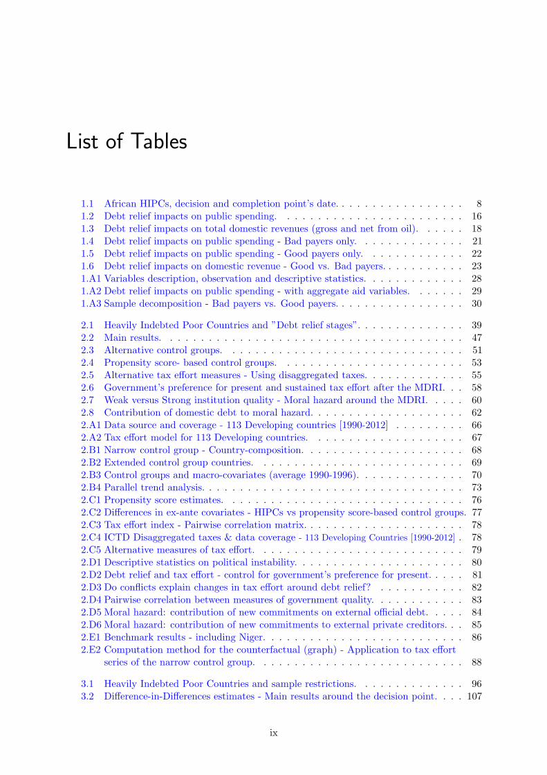
List of Tables

1.1 African HIPCs, decision and completion point’s date. . . . . . . . . . . . . . . . . 81.2 Debt relief impacts on public spending. . . . . . . . . . . . . . . . . . . . . . . . 161.3 Debt relief impacts on total domestic revenues (gross and net from oil). . . . . . 181.4 Debt relief impacts on public spending - Bad payers only. . . . . . . . . . . . . . 211.5 Debt relief impacts on public spending - Good payers only. . . . . . . . . . . . . 221.6 Debt relief impacts on domestic revenue - Good vs. Bad payers. . . . . . . . . . . 231.A1 Variables description, observation and descriptive statistics. . . . . . . . . . . . . 281.A2 Debt relief impacts on public spending - with aggregate aid variables. . . . . . . 291.A3 Sample decomposition - Bad payers vs. Good payers. . . . . . . . . . . . . . . . . 30

2.1 Heavily Indebted Poor Countries and ”Debt relief stages”. . . . . . . . . . . . . . 392.2 Main results. . . . . . . . . . . . . . . . . . . . . . . . . . . . . . . . . . . . . . . 472.3 Alternative control groups. . . . . . . . . . . . . . . . . . . . . . . . . . . . . . . 512.4 Propensity score- based control groups. . . . . . . . . . . . . . . . . . . . . . . . 532.5 Alternative tax effort measures - Using disaggregated taxes. . . . . . . . . . . . . 552.6 Government’s preference for present and sustained tax effort after the MDRI. . . 582.7 Weak versus Strong institution quality - Moral hazard around the MDRI. . . . . 602.8 Contribution of domestic debt to moral hazard. . . . . . . . . . . . . . . . . . . . 622.A1 Data source and coverage - 113 Developing countries [1990-2012] . . . . . . . . . 662.A2 Tax effort model for 113 Developing countries. . . . . . . . . . . . . . . . . . . . 672.B1 Narrow control group - Country-composition. . . . . . . . . . . . . . . . . . . . . 682.B2 Extended control group countries. . . . . . . . . . . . . . . . . . . . . . . . . . . 692.B3 Control groups and macro-covariates (average 1990-1996). . . . . . . . . . . . . . 702.B4 Parallel trend analysis. . . . . . . . . . . . . . . . . . . . . . . . . . . . . . . . . . 732.C1 Propensity score estimates. . . . . . . . . . . . . . . . . . . . . . . . . . . . . . . 762.C2 Differences in ex-ante covariates - HIPCs vs propensity score-based control groups. 772.C3 Tax effort index - Pairwise correlation matrix. . . . . . . . . . . . . . . . . . . . . 782.C4 ICTD Disaggregated taxes & data coverage - 113 Developing Countries [1990-2012] . 782.C5 Alternative measures of tax effort. . . . . . . . . . . . . . . . . . . . . . . . . . . 792.D1 Descriptive statistics on political instability. . . . . . . . . . . . . . . . . . . . . . 802.D2 Debt relief and tax effort - control for government’s preference for present. . . . . 812.D3 Do conflicts explain changes in tax effort around debt relief? . . . . . . . . . . . 822.D4 Pairwise correlation between measures of government quality. . . . . . . . . . . . 832.D5 Moral hazard: contribution of new commitments on external official debt. . . . . 842.D6 Moral hazard: contribution of new commitments to external private creditors. . . 852.E1 Benchmark results - including Niger. . . . . . . . . . . . . . . . . . . . . . . . . . 862.E2 Computation method for the counterfactual (graph) - Application to tax effort

series of the narrow control group. . . . . . . . . . . . . . . . . . . . . . . . . . . 88

3.1 Heavily Indebted Poor Countries and sample restrictions. . . . . . . . . . . . . . 963.2 Difference-in-Differences estimates - Main results around the decision point. . . . 107

ix

3.3 Difference-in-Differences estimates - Main results around the interim period. . . . 1083.4 Difference-in-Differences estimates - Gradual effect of debt relief. . . . . . . . . . 1143.5 Did financial environment in HICs trigger private capital flows to HIPCs? . . . . 1173.6 Debt relief additionality and changes in traditional official flows. . . . . . . . . . 1193.7 Debt relief additionality - bilateral vs. multilateral donors. . . . . . . . . . . . . . 1203.A1 Descriptive Statistics - Whole sample (112 DCs) [1992-2015] . . . . . . . . . . . . 1223.A2 Explanatory variables: expected effects on official financing conditions (and related

literature). . . . . . . . . . . . . . . . . . . . . . . . . . . . . . . . . . . . . . . . . 1233.A3 Explanatory variables: expected effects on financing to private creditors (and

related literature). . . . . . . . . . . . . . . . . . . . . . . . . . . . . . . . . . . . 1243.A4 Descriptive statistics on official financing flows. . . . . . . . . . . . . . . . . . . . 1253.B1 ”Extended” control group countries. . . . . . . . . . . . . . . . . . . . . . . . . . 1263.B2 Pre-Debt relief period: Descriptive statistics on covariates. . . . . . . . . . . . . . 1273.B3 Pre-Debt relief period: Descriptive statistics on outcome variables. . . . . . . . . 1283.B4 Event-Study - Test for parallel trends prior debt relief. . . . . . . . . . . . . . . . 1293.C1 Alternative selection criteria, alternative control groups. . . . . . . . . . . . . . . 1303.C2 DID estimates - Sensitivity to the narrow control group. . . . . . . . . . . . . . . 1313.C3 DID estimates - Sensitivity to the narrow control group (continued). . . . . . . . 1323.C4 Falsification tests. . . . . . . . . . . . . . . . . . . . . . . . . . . . . . . . . . . . . 1333.C5 DID estimates w/r to the extended control group. . . . . . . . . . . . . . . . . . 1343.C6 DID estimates w/r to the extended control group (continued). . . . . . . . . . . . 1353.C7 DID estimates - Outliers and sample sensitivity. . . . . . . . . . . . . . . . . . . . 1363.C8 DID estimates w/r to the extended control group - Bilat. donors. . . . . . . . . . 1373.C9 DID estimates w/r to the extended control group - Multi. donors. . . . . . . . . 1383.C10Investigating heterogeneity in HIPCs’ market access. . . . . . . . . . . . . . . . . 139

4.1 Summary statistics. . . . . . . . . . . . . . . . . . . . . . . . . . . . . . . . . . . 1474.2 Baseline estimations of the impact of tax on firm growth. . . . . . . . . . . . . . 1494.3 Investigating the ”granular hypothesis” in developing countries. . . . . . . . . . . 1514.4 Additional macroeconomic covariates and TSLS estimations. . . . . . . . . . . . 1554.5 Summary statistics on disaggregated taxes. . . . . . . . . . . . . . . . . . . . . . 1594.6 Impact on growth of resource and non-resources taxes. . . . . . . . . . . . . . . . 1604.7 Impact of taxation on growth depending on corruption. . . . . . . . . . . . . . . 1624.8 Prevalence of corruption by income groupa. . . . . . . . . . . . . . . . . . . . . . 1634.9 Effect of taxation according to firm-level characteristics. . . . . . . . . . . . . . . 1654.10 Channel of public good provision. . . . . . . . . . . . . . . . . . . . . . . . . . . . 1684.A1 Baseline estimations of the impact of tax on firm productivity growth. . . . . . . 1724.A2 Additional firm covariates and TSLS estimations. . . . . . . . . . . . . . . . . . . 1734.A3 Firm fixed effect estimations. . . . . . . . . . . . . . . . . . . . . . . . . . . . . . 1744.A4 Intensities by sectors. . . . . . . . . . . . . . . . . . . . . . . . . . . . . . . . . . . 1754.A5 Channel of public good provision. . . . . . . . . . . . . . . . . . . . . . . . . . . . 1764.B1 Sample of study. . . . . . . . . . . . . . . . . . . . . . . . . . . . . . . . . . . . . 1784.D1 Estimations with alternative fixed effects specifications and clusters. . . . . . . . 1804.D2 Estimations on regional sub-samples. . . . . . . . . . . . . . . . . . . . . . . . . . 1814.D3 Dropping one country at a time. . . . . . . . . . . . . . . . . . . . . . . . . . . . 1824.D4 Dropping one sector at a time. . . . . . . . . . . . . . . . . . . . . . . . . . . . . 1834.D5 Sensitivity to firms’ characteristics. . . . . . . . . . . . . . . . . . . . . . . . . . . 1844.D6 Random draw of firms. . . . . . . . . . . . . . . . . . . . . . . . . . . . . . . . . . 185

x

General Introduction

Development is costly. Whether it is domestically or externally financed, economic develop-

ment has always required the mobilization of large amounts of money. Yet the necessity to satisfy

basic needs of most vulnerable people and the MDGs’ achievement have drastically accentuated

financing needs of low-income countries (LICs) over the past decades. Unfortunately this is not

about to change. Climate change —already under way— and its dramatic consequences have

led the international community to reshape the way we thought about economic development

until then, and define new paths towards a more sustainable development.

The 2015 conference on Financing for Development (FfD) in Addis Ababa hence stressed the

need for additional financing intended to help developing countries in facing these new challenges.

The Sustainable Development Goals (SDGs) agenda, adopted few months later, now call both

developed and developing countries to step in and raise massive amounts of resources in order

to finance these goals. As stated by World bank’s president Jim Yong Kim in Addis Ababa,

SDGs will only be achieved by “substantially increasing funds for the world’s poor, moving from

billions to trillions of dollars in development spending”.6

The Addis Ababa Action Agenda (AAAA) —derived from this conference— lists several

areas where substantial improvements would help reaching such financing objectives. First,

focusing on domestic resources, the AAAA put taxation back to the center stage, highlighting

the necessity for developing countries to base their development process on fair and performing

tax systems. Second, and alongside domestic revenue mobilization, private sector development

is expected to take up an active role throughout the coming years, and to be supported with

international private capital flows such as foreign direct investment, particularly in key sectors

for sustainable development. Third, the AAAA has confirmed international aid and other

official flows as crucial factors in helping poor countries to strengthen domestic environment

and build essential infrastructures. Last, both domestic and external borrowing are encouraged

to significantly increase but without threatening the debt sustainability of poor countries in

order to prevent further episodes of debt distress. As a result, the AAAA restated the pivotal

role of the international community in assisting developing countries to attain long-term debt

sustainability through coordinated policies such as debt relief, restructuring and sound debt

management.

These four essays fall within this debate about financing for development and seek to provide

understandings about the effectiveness and consequences of two major financing sources for

6http://www.worldbank.org/en/news/speech/2015/07/13/third-international-conference-financing-development

xi

LICs: debt relief and taxation. While one might think that these two financing instruments are

fundamentally different, they are intrinsically related, as chapter 1 and 2 try to show. Chapter

1 investigates the effects of debt relief on beneficiary government’s budget. Using time series

analysis, we try to identify the impact of debt service savings stemming from debt relief on various

budget components such as public investment, current expenditures, and domestic revenues.

Chapter 2 builds on chapter 1 findings and takes a close eye to the relationship between debt

relief and taxation by focusing on tax effort evolution throughout the debt relief process. The

analysis also aims at understanding the role of recipient governments in this connection and

how their peculiarities affect outcomes of the debt relief programs. The third chapter reviews

challenges and opportunities that beneficiary governments face as regards external financing once

they have been granted debt relief. Lastly, after having exposed the importance of debt relief for

domestic revenue mobilization, chapter 4 proposes to go one step further by investigating the

effect of taxation on economic growth. Adopting a macro-micro approach, this essay intends to

revisit the taxation-growth nexus using firm-level observations in developing countries.

This general introduction starts with a brief overview of historical and recent evolutions in

development financing. Section 2 builds on these evolutions to narrow the discussion on the Third

World debt crisis of the 1980s-90s and the resulting multilateral debt relief initiatives of the early

2000s. After a short discussion about the expected effects of such initiatives, section 3 slightly

departs from debt relief to provide some element of context about the taxation-development

nexus and the related literature. The last section exposes the motivations of this thesis and its

structure.

0.1 Filling up the (double) resource gap

How to finance development? LICs can resort to various strategies which can be differentiated

according to their external or domestic feature. Domestically, countries can first seek to increase

savings, making funds available to support domestic investment and capital accumulation.

However, LICs are often characterized by quite narrow and unbalanced domestic capital markets

where most of the financial sector’s liquidities are absorbed by the public sector, thus leaving

limited opportunities for the financing of small and medium private activities. In addition, the lack

of strong value-added processes make it hard to redistribute wealth through the credit channel.

Therefore, in spite of the recent development of LICs’ financial sector and the mushrooming of

banking activities, most of the households and small enterprises still resort to informal financing

instruments with limited scope as regards development financing. As a result, domestic savings

have been hardly solicited to finance development of poorer economies over the past decades,

although recent trends suggest that it is about to change.

Taxation hence appeared as the sole alternative for domestic financing. Historically, taxation

has always been advocated as a stepping-stone for economic development (Burgess and Stern

(1993), Besley and Persson (2007)). As underlined by Kaldor (1962) in the early 1960s “The

importance of public revenue to the underdeveloped countries can hardly be exaggerated if they

are to achieve their hopes of accelerated economic progress”. Fifty years later, the OECD (2010)

restated his argument, claiming that “development success stories go hand in hand with better

xii

mobilization of a country’s own resources and less dependence on foreign finance”. Yet taxation

hardly took off in developing countries due to many structural constraints such as narrow tax base

and weak fiscal capacity that hampered the establishment of efficient and fruitful tax systems.

Alongside these issues, bad design of fiscal policies and governments’ misuse of public resources

prevented to set up a strong “fiscal contract” with taxpayers and to foster tax compliance

which consists in one of the main impediments to domestic resource mobilization in developing

countries. Despite the efforts deployed by LICs’ governments —coupled with those of the IFIs’

to improve taxation—, most of these countries painfully managed to levy more than 15 percent

of their GDP as fiscal resources, and still experience low tax ratios (Besley and Persson, 2014).

LICs thus logically turned towards external sources. Given their need in foreign currency

—necessary to finance imported goods that most of the LICs are unable to produce domestically—

trade consisted in a promising solution for developing countries. Regarding LICs openness rates

—which are often larger than those observed for high-income countries—, it seems fair to say that

LICs, and developing countries to a larger extent, have succeeded in inserting the globalization

process. International trade thus partly contributed to fill this foreign currency gap. In addition,

imports significantly contributed to increase domestic resource mobilization by facilitating tax

collection at the borders, which is however doomed to reduce in a today’s context of greater

regional and global integration. However, although beneficial for their development, exports

were —and for some countries still remain— not enough to help rapidly grow, mostly because

of the low diversification of their economic base. Besides trade, foreign direct investment also

consisted in an interesting solution for developing countries’ financing. Marginal in the late 1980s,

foreign capital inflows substantially increased starting from the 1990s, and helped in providing

substantial amounts of foreign currency but also technology and skills to recipient countries

(Dabla-Norris et al., 2010). Yet despite a recent broadening in FDI destinations —reflecting the

growing economic globalization and the proliferation of market-oriented reforms in LICs—, the

first waves of foreign capital inflows were more often targeted to countries with large mining and

extractive sectors, rather than resource-poor countries. Although the recent trends coupled with

the AAAA recommendations let us think that FDI might be of crucial importance for LICs’

financing in the coming years, such inflows were historically not sufficient to close the financing

gap of these countries, which was potentially compensated —but most often incompletely and

for some LICs only— by large inflows of remittances. In overall the lack of foreign currency

remained substantial for most of developing countries before the 1990s.

Therefore, from the independences on, LICs facing this double gap had no other solution

than turning towards external borrowing. Initiating their take-off, most of the LICs in the late

1960s were however de facto excluded from international financial markets. External support

thus mainly came from Bretton Woods Institutions and high-income countries’ governments,

most of which were keeping strong ties with their former colonies. Moreover, having realized the

particular needs and borrowing constraints of LICs —and the lending risk associated with it

(Humphrey, 2016)—, the international financial institutions (IFIs) created special subsidiaries

intended to provide concessional financing for LICs’ development. The World bank thus created

the International Development Association (IDA) in 1960, which was followed by the Structural

Fund Adjustment set up by the IMF in 1986. From the mid-1970s onwards, financial flows from

xiii

multilateral and bilateral donors towards LICs rapidly increased, except between 1992 and 2000

which corresponded with the “aid-fatigue” period.

At the end of the 1980s, most of the LICs’ financing was thus supported by IFIs, bilateral

donors, and in a lesser extent international commercial banks for countries exposing sufficient

guarantees to make banks lend them. Yet, despite all these efforts, many were still stuck in what

Sachs labeled a ”poverty trap”. All the more detrimental, and without being able to say whether

the billions of USD provided as foreign aid had been effective in achieving sustained higher

economic growth and lifting people out of the poverty, the public finance situation of recipient

countries became genuinely worrisome at the end of the 1980s, thus calling for substantial debt

relief.

0.2 Debt relief: the unwanted child

“What Africa needs to do is to grow, to grow out of debt.”

Dr. George Ayittey, President of the Free Africa Foundation.

0.2.1 How did we get there?

Debt issues in low income countries began in the early 1970s and spread over almost three

decades. The reasons for the impressive debt accumulation in LICs have been investigated quite

extensively by the literature of the 1980s which identifies three main developments over the 1970s

and the 1980s that initiated the third world’s debt crisis (Krumm, 1985; Lancaster et al., 1986;

Greene, 1989): i) the sharp increase in commodity prices during the 1970s which inflated exports

revenue and enabled LICs’ governments to contract loans intended to finance massive domestic

projects; ii) the subsequent burst of the commodity bubble which called for additional borrowing

in order to sustain development projects started up few years before, and iii) bad decisions from

debtor governments as regards the use of external financing and the design of these projects,

for the most part ill-conceived. Among the peripheral and exogenous factors that also fueled

this crisis, the rise in FED interest rates after the second oil-shock was often put forward, but

only concerned the few LICs that had succeeded to borrow from commercial banks during the

commodity boom. Simultaneously, the early 1980s severe drought encountered by sub-Sahara

African countries yielded most of these countries to increase grain imports financed by external

debt (Krumm, 1985; Greene, 1989). Yet, according to Mistry (1991), although debtors failed to

profit from these financial inflows, official creditors were also to blame given their irresponsible

financing policy during the 1970s that consisted in over-lending to LICs. Underlining the lenders’

impressive passivity, Mistry (1991) argues that their inaction helped arrears to accumulate up to

the point where repaying them would have been too costly for debtors, letting thus debt relief as

the only conceivable solution.

By the end of the 1980s, the sole debt of sub-Saharan African countries amounted to USD

136 billion while it was only USD 6 billion in 1970, thus consisting in an increase by around

630% (in constant USD) (Greene, 1989). While UNCTAD diagnosed the debt distress of the

LICs in the late 1970s, it took ten years for debt relief to be granted. The first moves were

purely bilateral and quite disorganized until the Paris Club stepped in to coordinate. Yet, the

xiv

initial debt treatments failed to halt the LICs’ increasing debt burden. Indeed, debt treatments

under the “classic terms”, the first wave of treatments granted in the Paris Club, only aimed at

rescheduling debts contracted prior a given cut-off date and at non-concessional interest rates,

which just postponed payment issues. Consequently, Paris Club treatments became increasingly

favorable by providing up to 33% and 50% reduction in bilateral debt service respectively under

the Toronto terms in 1988 and the London terms in 1991.

Despite these first two waves of coordinated debt treatments, the average stock of external

public debt for the heavily indebted and poor countries (HIPCs) reached frightening levels in the

mid-1990s. The Paris Club thus decided to go further and raise the reduction up to 67% under

the Naples terms, extending it to the entire stock of bilateral debt claims. This —combined with

ad hoc strategies such as fresh-money for LICs allowing them to buy their debt back to private

creditors— finally succeeded in reversing the indebtedness dynamics.

0.2.2 The multilateral debt relief initiatives: design and expected effects

However, the various actions of the Paris Club still left multilateral debt weighing on LICs’

public finance. Furthermore, alongside these bilateral treatments, multilateral organizations

continued to grant concessional loans for development projects (Leo, 2009) and for sums far

greater than the canceled debts (Easterly, 2002) such as that HIPCs’ net transfers were still

positive in 1995 (Thugge and Boote, 1997), hampering thus their deleveraging process (Leo,

2009).

Therefore, in 1996, the G7 decided to expand bilateral debt relief up to 80% under the

Lyon terms and most importantly, broke with the principle of untouchable multilateral debts by

setting up a debt relief programme known as the Heavily Indebted Poor Countries Initiative

(HIPC). Under the first HIPC initiative, launched in 1996, eligibility criteria allowing countries

to benefit from debt relief were relatively precluding. Besides being ranked as a LIC by the

World bank, and having implemented an macro-stabilizing program (PRGF), countries had to

record a debt-to-exports ratio superior to 250% in present value (PV) to be eligible for the debt

relief program. Yet this ratio prevented some countries to benefit from the initiative although

facing significant difficulties in meeting their heavy debt service payments. The international

community therefore decided in 1999 to raise bilateral debt cancellation up to 90% (under the

Cologne terms), reduce the debt threshold down to 150% of the exports (250% of domestic

revenue for really open economies), speed up debt relief provision, and thus renamed the original

HIPC initiative, the “Enhanced” HIPC initiative.

The Enhanced HIPC initiative is designed as a stepwise process. Once eligible, the country

reaches the decision point where the government benefits from debt service cancellations and,

according to the conditionality attached to the initiative, starts implementing (alongside the

PRGF undertaken for being eligibility to the program) a poverty-reduction program (PRSP)

entailing specific goals to meet over the medium-run. As long as the country is considered on

track in regard to poverty reduction, program’s stakeholders continue to grant debt service

relief. The resulting debt service savings thus fuel a specific public account entirely (in theory)

dedicated to the financing of development projects lined up on the goals defined within the

PRSP. Once the country has met these goals, the completion point marks the end of the HIPC

xv

process and grants irrevocable debt stock cancellations on which the debtor government and

program’s stakeholders previously agreed on.

Yet, although debt relief provided under the Enhanced HIPC initiative was substantial

(especially for bilateral donors), multilateral liabilities, though being reduced, were still weighing

on governments’ budget, slowing down the race toward the MDGs. Consequently, Bretton

Woods institutions and the regional development banks (AfDB, IADB) decided in 2005 at the

G8 summit of Gleneagles, to cancel the entire remaining multilateral debt stock of HIPCs that

have completed the initiative. This ultimate debt relief program known as the Multilateral

Debt Relief Initiative (MDRI) therefore involves, since 2005, the full cancellation of outstanding

multilateral debt for countries that have reached their completion point under the Enhanced

HIPC initiative.

To date, the HIPC and MDRI initiatives have written off a total of nearly USD 76 billion.

These cancellations of the external debt of 39 LICs may seem a pittance compared with relief in

middle- and high-income countries, but are huge in relative terms. They represent just over all

the subsidies granted to all the HIPCs in constant dollars from 2009 to 2011.

0.2.3 What can we expect from debt relief?

What have been the motivations to cancel such amounts of debt? Obviously, these initiatives

have not only been implemented for the simple purpose of restoring debt sustainability among

LICs and writing off bilateral and multilateral claims that were —for some of them— already

forgot by their sharer. The goal of these programs aimed to go beyond the simple cleaning

process by providing development opportunities which were until now restrained because of the

heavy debt burden. Indeed, from a theoretical standpoint, it is relatively accepted that too

much government debt undermines economic growth. This idea, which owes its paternity to the

seminal work of Krugman (1988) and Sachs (1989) in the late 1980s, is currently known as the

“Debt Overhang” theory (DOT).

In his paper of 1988, Krugman (1988) posits that a debt overhang situation arises when the

indebtedness level is such that it becomes beneficial for both the debtor and its creditors to

cancel a share of the debt. He underlines that, in the presence of large indebtedness, incentives

of the debtor to reimburse might be distorted, resulting in lower capacity to pay, increase in the

likelihood of partial default, and thus in reduction of debt market value.

Incentive and liquidity effects

Using a two-period model, Krugman (1988) shows that temporary concessional financing

can solve liquidity as well as solvency issues of the debtor, leading creditors to be better off as

compared with a full default situation. He argues that such concessional financing would help

debtor countries to face their short-term debt payments and undertake substantial investment

efforts yielding additional revenue in the next period, and hence making debt easier to service.

However, this argument relies on the assumption that the debtor gives away to its creditors all

the resources it can generate in order to repay its debt. Yet, as underlined by Krugman (1988)

and Sachs (1989), if the debt burden is such that repayments equal the maximum the country can

pay with the largest adjustment effort “there is no reason for the country to make the adjustment

xvi

effort, since the reward goes only to its creditors” (Krugman (1988), pp.14). In such situation,

debt relief can solve the problem. Sachs (1989) shows that creditors can partially cancel the

claims they have on the debtor down to the level where the resulting debt repayments would be

inferior to the stream of revenue stemming from the adjustment effort undertaken by the debtor.

It would then allow the debtor to partially benefit from the outcomes of its adjustment efforts,

and would secure a non-zero payment for creditors as compared with a situation of full default.

Other detrimental effects stemming from a debt overhang have been emphasized by Boren-

sztein (1990) and Claessens and Diwan (1990) for which large stock of debt can discourage

national and foreign investors since it suggests further rise in taxation intended to service the

debt, thus pushing future production costs upward. In addition, Borensztein (1990) states

that credit rationing induced by unsustainable levels of public debt can also be detrimental for

domestic investment. Debt relief should thus be accompanied with extra lending, and thus be

additional, in order to maximize the impact on the investment-to-GDP ratio. Therefore, since

large debts depress investment by creating negative incentives to undertake pro-growth reforms

for public entities and to invest for private agents, debt relief should foster both public and

private capital accumulation, yielding in fine to larger economic growth rates.

Besides these potential incentive effects, Claessens and Diwan (1990) underline that in LICs,

where consumption and investment intended to basic needs can hardly be reduced, large debt

burden let the adjustment weighs on debt service repayments which can be only partial. But

considering a worst scenario for the debtor, Sachs (1989) argues that debt reschedulings and

pressures from donors can force the debtor to service its debt, leading to crowd public funds

(initially intended to domestic development projects) out. In this case, debt relief enables debtors

to free up sums previously spent on debt service and thus generates “fiscal space” (Heller,

2005), which materializes only if government was repaying its debt (at least partially) prior debt

cancellations (Cohen, 2001).

Disincentive effects

Yet while these studies support the idea that debt relief can foster government and private

investors to undertake significant investment efforts, some authors support that debt relief could

also create disincentives to invest. For instance, Corden (1989) first defines a three-period model

where if the debtor cannot pay in period 2 its inherited debt from period 1, concessional financing

provided by the creditor in period 2 to service this debt, must be repaid in period 3. Under these

settings, he explains that debtor country would deploy significant investment effort in period

1 and 2 to generate revenue in order to pay the difference between debt service and defensive

lending in period 2, and to reimburse liabilities contracted in period 2 and due for period 3. In

presence of debt relief, Corden (1989) shows that investment effort in period 2 would be lower

since there is nothing to service anymore. In addition, although this reduction in investment

leads to lower output in period 3, resource transfers abroad fall so much after debt relief that the

debtor’s consumption actually raises as compared with the situation where the country would

have paid its debt. But as for the illustration of Krugman (1988), this example assumes the

debtor’s willingness to pay to be maximal, which remains hardly debatable.

xvii

Debt relief and conditionality

Others authors thus argue that debt relief can result in higher growth and repayment

equilibrium only if both parties commit themselves to necessary future actions (Claessens and

Diwan, 1990). On the one hand, creditors must commit that they will not ask for too much

resource transfers from the debtor in the future, which can be achieved by combining concessional

loans with debt relief. One the other hand, debtor must ensure to invest revenue stemming from

debt cancellations in an efficient way by prioritizing profitable and resource-creating projects.

Such actions can be achieved through conditionality and adjustment programs imposed by the

IFIs, which in the context of LICs, often represent their creditors.

The authors also state that in a “weak debt overhang” scenario, situation can improve

with a simple commitment mechanism ensuring that new loans will be efficiently used and will

generate enough revenue to service this new debt. However, if the debtor cannot commit to

these adjustment efforts, creditors will have no other choice than resorting to debt relief. Indeed,

in a context of “strong debt overhang”, new loans will not be enough to convince the debtor to

undertake resource-creating investment for future debt servicing. It will consider adjustment

efforts only if creditors agree to partially cancel their claims, since in this case, only a fraction of

the gains derived from this effort will go to the creditors.

Sachs (2002) accentuates this idea and suggests debt relief to be always associated with

conditionality and new IFIs lending since it yields debtor countries to a better equilibrium

(depending on its discount rate), leading them to always comply with conditionality. Lastly,

Koeda (2008), supports the idea that highly indebted countries lying below a certain income

cutoff (the one that graduates from low-income to lower-middle income country) have strong

incentives in favoring short-term consumption over investment to stay below this cutoff and

continue borrowing at concessional terms. According to Koeda (2008) debt relief should consist

in a one-shot strategy in order to prevent moral hazard in LICs which would be disposed

to postpone pro-growth reforms, consume inefficiently and accumulate debt again since they

anticipate future debt cancellations on the same eligibility criteria.

∗

In overall, theoretical papers addressing the debt-growth nexus seem to converge towards

the same idea that high level of debt is detrimental to economic growth, making thus debt relief

an efficient development strategy for countries stuck in poverty trap. Yet, while some authors

strongly stand in favor of conditional debt relief in order to ensure that incentives and liquidity

effects result in sustained higher growth, others also stress the potential moral hazard that such

actions could generate. Adopting various empirical approaches, the first three essays of this

thesis try to modestly shed some lights on these effects which, among the existing literature,

have either not been clearly set yet or even investigated.

xviii

0.3 Taxation: the cherished son

“The real spelling of aid is t.a.x.”

Jeffrey Owens, former head of tax at the OECD (2001-2012).

Vice-president of Seychelles Danny Faure stated at the 2015 Addis-Abbaba conference,

that given the former developments as regards debt in sub-Sahara Africa and small island

countries, “debt restructuring and cancellations coupled with sound fiscal and monetary policies,

is an essential tool for financing for development”.7 Though debt relief is expected to improve

taxation through its incentives effects or conditionality, one could however wonder whether the

AAAA’s top priority (taxation) does not conflict with other objectives such as private sector

development.

0.3.1 Taxation and development

Since the early 60s, taxation has been increasingly accepted as a fundamental pillar of

the economic development process (Kaldor and Kaldor, 1965; Tanzi, 1983, 1992; Burgess and

Stern, 1993). Most of development actors have acknowledged that although growing financial

needs of LICs could not be entirely fulfilled with domestic resources and that foreign financing

was strongly needed, taxation was essential to the state building process (Besley and Persson,

2007, 2010, 2013). Consequently, for decades, LICs and international institutions have deployed

increasing endeavors to design, set up and foster tax systems across the developing world.

Yet, first theoretical works have shown that taxation could negatively affect the way in

which the economy converges towards its long-run equilibrium (Feldstein, 1974; Chamley, 1986;

Judd, 1985). In particular, an important theoretical body building on the neoclassical models

of investment (Jorgenson, 1963; Tobin, 1969; Hayashi, 1982) shows that taxation influence the

global economic activity mainly through its micro effects on firm investment decisions (Hall

and Jorgenson, 1967; Summers et al., 1981; Auerbach et al., 1983), identified as detrimental for

investment behavior and business incentives.

However, departing from a benchmark situation similar to a high income economy, such

conclusions cannot be taken for granted when it comes to developing countries. Indeed, as

demonstrated by Barro (1990) in a growth model with a balanced government budget, the

contribution of public spending (hence of taxation) to capital accumulation mostly depends

on government’s size and the marginal returns of such expenditures. In keeping with Barro’s

intuitions, while tax raise reduces economic growth, extra public spending derived from higher

tax effort, should help the country to grow faster if its marginal returns are substantial, which

is likely to be the case in the context of developing countries where there is a significant lack

in infrastructure. Yet, as underlined by (Aghion et al., 2016), such positive effect of taxation

are only possible if domestic revenue efficiently translate in efficient public spending such as

infrastructures, which also depends on the institutional environment and government’s political

accountability in particular.

7http://www.un.org/esa/ffd/ffd3/wp-content/uploads/sites/2/2015/07/seychelles.pdf

xix

0.3.2 Taxation in the Financing for Development agenda

Historically, the first involvement of the international community into developing countries’

tax system occurred with the repeated expert assessments of Edwin Kemmerer in Latin America

between 1917 and 1931 who mainly advised reorganization of the financial sector and reforms of

public finance (Alacevich and Asso, 2009). This then took another step with the Shoup mission

of 1949 which sent seven US economists to the post-World War II Japan in order to get the tax

system back on a solid ground. The success of this intervention led for the next two decades

the IFIs to send influential economists in developing countries to improve existing tax systems.

However, starting from the 1980s, Bretton Woods institutions stopped relying on small groups of

leading individuals and started to promote the development of tax systems in recipient countries

by tying their disbursements to structural reform programs. As a matter of fact, 1980s’ SAF

programs mainly targeted public deficit reduction by promoting increases in domestic revenues

and wise control over public spending (Ghosh et al. (2005)). These efforts slowed down during

the “aid fatigue” period, but started again in the early 2000s with increasing involvements from

bilateral donors which also began to develop tax-related official assistance (Fjeldstad, 2013).

Nowadays, given the increasing financial needs stemming from the MDGs and now the SDGs,

the international community is fully committed to support taxation in developing countries

which also contributes to improve the well-functioning of the state (Kaldor (1981)), to reinforce

its legitimacy and power (Di John (2009)) and, in a larger extent, fosters institutions quality and

democracy (Fjeldstad (2013), Besley and Persson (2013)) when external assistance is provided

in the right way.

Yet, and as exposed above, despite all this assistance, tax ratios in developing countries and

especially in Sub-Sahara Africa has remained significantly low over the past decades. Causes

are numerous and range from the insufficient tax base to the replication of tax systems in

countries where the economic environment was not appropriate to make such systems work

(Fjeldstad, 2013). Corrupted elites and weak public goods provision also contributed to maintain

low tax compliance since citizens cannot touch or even catch sight of benefits derived from

tax payments (Fjeldstad and Therkildsen, 2008). Indeed, in many developing countries, public

finance mismanagement and rent-seeking behaviors fueled extractive institutions, supporting

high reliance on exports taxes, and thus monopolizing domestic resources for elites self-interest

which were more often directed to shady foreign bank accounts rather than to the local economy

(Boyce and Ndikumana (2011)).

Consequently, since July 2015 and the AAAA, many initiatives have been undertaken in

order to efficiently raise tax revenue in developing countries. These have focused on two kinds

of actions; expanding the tax base and fighting international tax evasion. As regards the first

objective, many efforts are currently deployed on the inclusion of informal activities into the

formal sector. In addition, specific strategies are directly addressed to resource-rich countries

which are encouraged to invest in value-addition within the processing of natural resource in order

to secure a pool of domestic revenue that does not depend upon international price fluctuations.

Tax base expansion for developing countries is thus considered as a necessity by the international

community, especially in a context of wider regional integration and diminishing custom duties

which represent, by far for some countries, a significant share of their domestic revenue. Besides

xx

tax base enlargement, lot of actions have also been undertaken in order to fight capital flights and

international tax evasion. International initiatives such as “Tax Inspectors Without Borders”,

the “Extractive Industries Transparency Initiative” (for resource-rich countries), the “Stolen

Asset Recovery Initiative” as well as supra-national-level committees or forums on tax issues

have multiplied in the recent years, underlining the need to address both sides of evasion; evaders

and host institutions. This has been set in order to drastically limit capital flights which dry the

tax base of developing countries up, keeping most of them aid-dependent and hampering the

implementation of enduring and efficient tax systems.

∗

The last essay of this thesis falls within this debate about the pivotal role of taxation for

economic development. Although stressed as a necessary mean for the attainment of the SDGs

by 2030, one may wonder if, in view of the theoretical literature exposed above, significant

raise in taxation might conflict with other AAAA’s recommendations such as the expansion

of the private sector. Still, only few studies have tried to observe the impact of taxation on

firm performance in the particular context of developing countries (Easterly and Rebelo, 1993;

Djankov et al., 2010; Fisman and Svensson, 2007). The essay thus aims at filling this gap in the

literature by empirically investigating this relationship.

0.4 Chapters’ summaries

As highlighted throughout the introduction, the debt overhang theory and the conditionality

associated with the multilateral debt relief initiatives suggest that debt cancellations might affect

public finance of recipient countries. Chapter 18, co-written with Marc Raffinot (University

Paris-Dauphine), Danny Cassimon (University of Antwerp, IOB), and Bjorn Van Campenhout

(IFPRI), thus focuses on the fiscal effects of debt relief in beneficiary countries. Considering

a sample of 24 HIPCs for which the post-debt relief period is long enough, we use time-series

analysis and panel VAR specifications to estimate the effects of debt service savings stemming

from debt relief on various fiscal outcomes such as public investment, current expenditures, and

taxation. Our empirical specification follows a basic government budget representation and then

investigates how components react to shock on one specific variable. Moreover, thanks to the

temporal depth of our sample, we are able to differentiate debt relief effects according to the

initiative under which cancellations have been granted. Results show that debt relief provided

under the Enhanced HIPC initiative fosters public investment while additional cancellations

under the MDRI increase public current expenditures.

We explain the positive contribution of the Enhanced HIPC initiative by the conditionality

attached to debt service relief where proceeds must be used to finance development-oriented

expenditures such as infrastructures in social sectors. However, the positive effect of debt relief

stemming from the MDRI is more difficult to interpret. On the one hand, such effect can simply

translate the increase in running costs of public investment undertaken through the Enhanced

8Published in International Economics in 2015, vol. 144.

xxi

HIPC initiative. On the other hand, this increase could also come out as a return to old policies

once full debt relief has been granted, leading beneficiary governments to reallocate public funds

toward sectors of political interests, which do not necessitate capital spending. Panel VAR

results then also underline a positive effect of debt relief granted under the Enhanced HIPC

initiative on domestic revenue mobilization which ties in with the debt overhang theory stating

that debtors are more prone to collect taxes once they are freed from their debt burden, since

tax effort benefits do not go to the creditors anymore. This transmission channel is considered

alongside the potential effect of conditionality under the Enhanced HIPC initiative, which clearly

requires improvements as regards domestic revenue mobilization.

The last section of chapter 1 investigates heterogeneity in beneficiary countries’ fiscal response

by differentiating HIPCs that were paying most of their debt prior the initiatives from those

that did not. Following Cohen (2001), one should expect to observe no or less fiscal space for

countries that were not fully repaying their debt prior debt relief. Using the ex-ante amounts

of debt stock arrears to distinguish bad payers from good payers, we find (in line with Cohen

(2001)) that bad payers experience no change in tax-to-GDP ratio but most importantly record

a lower fiscal space once they have been granted debt relief.

Chapter 2 builds on these findings to narrow the analysis to the relationship between debt

relief and tax effort. First computing tax effort index, which aim at representing the government’s

performance in collecting its potential taxes, I then investigate how government’s tax effort

evolve throughout the entire debt relief process (from the decision point to the MDRI). Using a

difference-in-differences approach, I start by identifying various groups of countries which, at the

macro-level, might represent a satisfactory counterfactual. After having carefully check for the

control groups’ suitability, I estimate tax effort changes around different stages of the debt relief

process and with respect to these various counterfactuals.

Results suggest that HIPCs deploy substantial tax effort beforehand in order to become

eligible for the Enhanced HIPC initiative. Such result is expected given the design of this

initiative which requires candidate countries to report satisfactory implementation of their

macro-stabilizing program before being able to reach the decision point. Findings then show

that higher tax effort is sustained throughout the period running from the decision point to the

MDRI (which corresponds to the completion point for most of the HIPCs considered in this

study). However, tax effort seems to reduce once full and irrevocable debt relief is provided

under the MDRI. Given that the completion point marks the end of the HIPC process and

therefore of its associated conditionality, HIPCs’ governments are then free to shape their fiscal

policy the way they want. Under such design, moral hazard is thus likely to materialized.

Regarding this suspicion of moral hazard, the analysis takes one step further and then tries

to identify the reasons for such easing off in tax effort after the MDRI. Results suggest that

governments are more prone to moral hazard when they highly value the present, here proxied by

political instability. Findings also show that inefficient governments as regards public finance and

economic policies management are those experiencing a significant drop in tax effort after the

MDRI. Lastly, additional results suggest that new financing opportunities stemming from debt

relief, such as the expansion of local debt markets, also tend to reduce tax effort for recipient

xxii

governments after the MDRI. This second chapter thus emphasizes moral hazard induced by the

carrot-and-stick design of these initiatives which leads some beneficiary countries to lose part of

the effort they gained throughout the debt relief process. However, despite such behavior, HIPCs

still managed to secure levels of tax effort that remain higher as compared with a situation

where they would not have benefited from such initiatives.

Chapter 3 then reviews changes in external public financing following debt relief programs.

This paper, co-written with Marc Raffinot (University of Paris-Dauphine) and Baptiste Venet

(University Paris-Dauphine) adopts a similar empirical approach as the one used for chapter

2, and seeks to estimate the evolution of borrowing conditions to official creditors as well as

access to international financial markets around different stages of the debt relief process, still

with respect to various control groups. We find that having benefited from debt relief under the

Enhanced HIPC initiative leads official creditors to tighten their lending conditions. In particular,

we observe that HIPCs experience a significant reduction in the average grace and maturity

periods on new official loans, yielding to a substantial fall in the grant element associated with

such financing. Simultaneously, results suggest that beneficiary countries managed to contract

loans to private creditors such as foreign commercial banks, hence gaining access to international

financial markets from which they were historically excluded.9

Going further, the last part of this paper investigates under which circumstances HIPCs

succeed in accessing financial markets. Findings suggest that HIPCs are more likely to con-

tract this kind of debts once they have received additional and irrevocable debt relief under

the MDRI, highlighting the private creditors’ appetite for countries without debt. Additional

analyses tend to show that private banks and other creditors are more disposed to lend during

financial bust in developed economies, hence suggesting as a potential transmission channel

the willingness of private investors to seek for higher market returns in developing countries;

among which those with a renewed borrowing capacity seem to be favored. Departing from

the “push factors”, last findings highlight that such resort to external private investors might

be motivated by substantial reductions in gross aid transfers from official creditors (in ad-

dition to the lending conditions’ tightening). This final result suggests that debt relief has

not been additional (at least as compared with control group countries), and that given the

financing needs of HIPCs, beneficiary countries had no other choice than finding new financing

sources, on average more costly, resulting in uncertainty as regards their future debt sustainability.

Lastly, chapter 4, co-written with Lisa Chauvet (IRD-DIAL), revisits the taxation-growth

nexus using a macro-micro approach. To this end, we match country-level data about taxation

from the Government Revenue Dataset (International Center for Taxation and Development)

which provides reliable information on taxation in developing countries, with firm-level data re-

trieved from the World Bank Enterprise Surveys (WBES). Using repeated cross-section estimates,

our findings support a non-linear relationship between taxation and firm growth, as predicted by

the theoretical literature and Barro (1990) in particular. However, although taxation benefit to

firms’ activity in developing countries, we find that a significant prevalence of corruption leads

9Although some of them managed to borrow from private creditors in the early 1980s.

xxiii

to reduce this positive effect, especially in low-income countries where the economic environment

remains unstable and domestic revenue mobilization is low. Lastly, making use of the firms

heterogeneity, and adopting a empirical approach similar to Rajan and Zingales (1998), we find

fragile evidence that the positive contribution of taxation to firm performance goes through the

provision of public goods since enterprises operating in sectors highly dependent on infrastructure,

benefit more from taxation.

∗ ∗ ∗

The purpose of this thesis is thus to provide new empirical evidences about the effect

of two financing strategies —debt relief and taxation— intended to support economic and

social development of poorer and most vulnerable countries. The four essays investigate some

relationships regarding these financing instruments —seperately or bridging the two— that

have not been extensively addressed by the existing literature or that did not led to consensus

among the scientific community. Each essay highlights new findings involving clear policy

recommendations that line up with the Addis Ababa Action Agenda and call for greater

coordination between all stakeholders of the development process.

xxiv

Chapter 1

Africa: Out of debt, into fiscal space?

Dynamic fiscal impact of the debt relief

initiatives on African Heavily Indebted Poor

Countries (HIPCs)

with Danny Cassimon, Marc Raffinot, and Bjorn Van Campenhout

Published in International Economics, 2015, vol. 144, p. 29-52.

1.1 Introduction

Low Income Countries (LICs) have been granted debt relief by bilateral creditors and later

by multilateral creditors under the Heavily Indebted Poor Countries (HIPC) Initiative for debt

reduction in 1996 and 1999, and from 2005 on under the Multilateral Debt Relief initiative

(MDRI). By December 2014, 36 countries have benefited from the HIPC initiative (IMF, 2000).

The HIPC initiative’s first goal was to cancel debt down to a level that would restore debt

sustainability. This was also supposed to eliminate the debt overhang. According to this theory,

a high debt burden depresses investment, reform willingness and, hence, future economic growth.

Furthermore, debt relief should allow some public resources, otherwise being used for debt

service, to be liberated for alternative use, which is the so-called ‘fiscal space’; donors were

to monitor the use of this money freed in order to make sure that this money was used to

increase poverty-reducing public spending. To be more specific, in the late 90s, donors insisted

that this money should be invested only in basic health care and primary education. Moreover,

conditionality attached to receiving the debt relief (and in particular at the completion point of

the HIPC initiative) should strengthen the probability of reaching the desired goals.

The rationale behind the MDRI is different, as it amounts to a full cancellation of the

remaining debt after HIPC due to the International Monetary Fund, The World Bank, the

African Development Bank and later also the Inter-American Development Bank. Nevertheless,

IDA and IMF made it compulsory to reach the HIPC completion point before benefiting from the

MDRI. By end-October 2013, 35 countries have benefited from the MDRI (Chad being the only

1

one that did not yet reach the completion point). For equity reasons, IMF also provided debt

relief under MDRI for Cambodia and Tajikistan, which did not previously benefit from HIPC

debt relief. These initiatives resulted in a dramatic decrease of the debt ratios of the benefiting

countries (cf. Figure 1.1 below). Even if IDA and IMF insist on an ongoing commitment to fight

poverty after HIPC completion point and MDRI, their monitoring is much weaker. As the debt

relief is irrevocable after this point (and because of the fiscal space thus created), the means of

pressure on the benefiting governments are limited.

While the fiscal space effects were of secondary importance in the HIPC Initiative, they

became central when donors decided to provide debt relief that went beyond HIPC, as through

the MDRI. Here, rather than aiming at restoring debt sustainability, the focus shifted more

towards providing recipient countries with additional resources to increase spending targeted

at realizing internationally-agreed poverty reduction targets such as the MDGs. However, the

resources freed by debt relief are a one- shot intervention. As such, improvements of tax collection

are needed in order to make this increase in public expenditure sustainable.

Figure 1.1: Evolution of average indebtedness (in face value) for 24 African HIPCs.

Notes: Data sources: International Debt Statistics (IDS), World Bank, downloaded the 03/06/2014.

Did this combination of debt overhang elimination, fiscal space and conditionality effects

led to positive effects on the fiscal situation of the recipient countries, in terms of higher

revenue, higher public investment or other public spending? The paper draws on earlier analysis

focusing on the ‘fiscal response’ effects of (HIPC) debt relief, and more notably on Cassimon

and Campenhout (2007); Cassimon and Van Campenhout (2008), and tries to complement the

preliminary findings of these studies by extending the time frame and using alternative estimation

2

techniques. Moreover, the extended time frame provides an opportunity to complement the

earlier studies by explicitly focusing for the very first time on the relative fiscal response effects

of the additional debt relief provided through the MDRI.

The reminder of this paper is structured as follows. In Section 2, we describe the channels

through which debt relief could affect fiscal variables, both in theory as in practice, referring to

the existing literature that links debt relief, economic growth and fiscal variables. The Section 3

deals with the data and the empirical specification we used for this study. Finally, Section 4

presents our empirical results. Section 5 concludes.

1.2 What should we expect from the HIPC and MDRI initiatives?

The main goal of debt relief granted by the donor community through the HIPC initiative

was canceling the debt down to a sustainable level, as defined by specific threshold indicators

of capacity-to-pay. This sustainable level was usually defined in balance of payments terms (a

present value of foreign debt to exports threshold), or in fiscal terms (a present value of debt

to fiscal revenue threshold) for very open economies. In order to be eligible (i.e. becoming an

HIPC), the country had to be IDA-eligible, and hold an unsustainable external debt. In 1999, the

initiative was enhanced by deepening debt relief and lowering the balance of payments and fiscal

thresholds to 150% and 250%, respectively. Implementation of the (Enhanced) Initiative followed

a two-phased approach: after some initial conditions met (e.g. a track record of successful IMF

program implementation), a country reached the so-called decision point, where creditors fixed

the amount of debt relief granted to the recipient HIPC ‘in principle’, after which the country

entered a second phase in which it had to fulfill a number of other country-specific conditions

(the so-called ‘triggers’, including the execution of a poverty reduction strategy), that would

ultimately lead to reaching completion point status, when the envisaged debt relief was granted

irrevocably. In between decision and completion point, the country already received (so-called

‘intermediary’) debt relief in the form of debt service relief on comparable terms as the debt

cancellation to be received at completion point.

1.2.1 The debt overhang predictions

The idea to cancel debt down to the sustainability level was not only to formally acknowledge

that these countries were not capable of (fully) servicing their debt and engaged in repeated

debt rescheduling that resulted in further stockpiling debt. It was also inspired by the so-called

‘debt overhang theory’ developed by Krugman (1988) and Sachs (1989). This theory states

that a high debt burden has a strong negative effect on the debtor country’s creditworthiness,

on investment behavior and on the capacity and willingness of these debtor governments to

undertake necessary but painful economic and institutional reforms (most of the benefits accruing

to external creditors). As such, canceling debt could have positive impacts on investment and

potentially on growth. The consequences of the debt overhang theory for debt relief programs

and their expected fiscal implications become then quite intuitive: eliminating debt overhang

would have a positive effect on public investment and could thus lead to larger fiscal revenue

stemming from the higher growth fueled by these additional investment. Moreover, according

3

to the debt overhang approach, it might also result in an increasing willingness for tax policies

implementation as it will directly benefit to the recipient country and no longer to the creditors.

Yet, the debt-growth nexus evidence so far is mixed. From an empirical perspective, many

studies (Elbadawi et al., 1997; Pattillo et al., 2011; Clements et al., 2003; Clemens et al., 2012;

Chowdhury, 2001; Presbitero, 2009, 2012) tried to test this debt overhang hypothesis and its

underlying non-linear relationship between debt, investment and growth.1 Results widely differ

according to the samples, the indicators (e.g. referring to stocks versus flows measures) and

the methodology used. Most papers dealing with this issue and finding significant nonlinear

relationships conclude that the negative impact of debt on national investment level (private and

public) remains negligible. Moreover, most studies rely on panel data mixing LICs and Middle

Income countries. However, by making specific assessments, Cordella et al. (2010) showed that

no impact of debt relief is to be observed on HIPCs.

1.2.2 Fiscal space: potential and real

Next to curing debt overhang, debt relief was supposed to provide debtor governments with

fiscal space resulting from money freed by debt relief. According to Heller (2005) definition,

there is fiscal space when a government experiences budgetary room which enables it to allocate

extra resources to specific purposes without threatening the sustainability of public finances. It

is however not straightforward that debt relief allows for direct fiscal space, and it is not easy to

measure it. First of all, a decision to cancel a given nominal stock of debt results in cash flow

gains distributed over a period of time, depending on the original debt service schedule. Second,

if the debt service due would not have been paid in the absence of debt relief, no cash flow

savings materialize (Addison, 2008). As in practice debt forgiven often would have been serviced

only in part, debt relief is more correctly measured as the gap between the new debt service and

the one that would have been serviced in the absence of debt relief (Cohen, 2001). In some cases,

the direct cash flow effect on recipient government resources may be close to zero; in others it

may be substantial. Third, when granting debt relief, donors may decide to cut back on their

other aid interventions, which may lead to no net fiscal space effects for the recipient countries.

For these reasons, we make a distinction in this paper between countries that were repaying

a significant part of their debt and countries that were not before debt relief. In the second

case, no fiscal space is likely to materialize. However, this distinction is not really easy to

implement as most HIPCs were running at least some arrears to some creditors. In particular,

some HIPCs were indebted to USSR, China, or even other African countries without being

pressed for repayment (a kind of de facto moratorium). In order to build our two sub-samples of

”good payers” and ”bad payers”, we use the ratio of arrears on external debt stock to the long

term debt stock (using the World Bank data) in 1995 (one year before debt relief under HIPC

initiative was made public - see Table 1.A3 in the Appendix).

1Following the ‘debt overhang’ theory, debt positively affects economic growth up to a particular threshold inthe debt-to-GDP ratio. After that, if this debt-to-GDP ratio increases further (and debt becomes unsustainable),debt would impact negatively on economic growth as described above. This indebtedness threshold would representthe turning point of a Laffer curve-type relationship between debt and growth (Krugman, 1988).

4

1.2.3 Fungibility and potential conditionality effects

Moreover, as is well known from the aid fungibility approach (Heller, 2005; Feyzioglu et al.,

1998; Van de Sijpe, 2013), benefiting governments could also try to optimally allocate the

resources saved, e.g. by cutting down domestic revenues (tax burden), or reducing the fiscal

deficit. All this means that it is not always granted that (HIPC) debt relief leads to more

resources available, and that they are being spent according to the donors’ objectives. It is

important to note the difference, at least in principle, between HIPC and MDRI debt relief.

HIPC debt relief might be considered partly fictitious, leading to little fiscal space effects. In

contrast MDRI debt relief should in principle be considered real resource savings that would

otherwise have been fully spent as actual debt service, because the pre-MDRI debt was supposed

to be sustainable. This is one specific feature that we want to test in this paper, complementing

existing research on this issue.

Moreover, according to the design of these debt relief initiatives, a conditionality effect

may be at play. Debt relief comes with some strings attached by donors. Enhanced HIPC

debt relief was granted after the successful completion of donor-imposed conditionality, some

comparable to an IMF program, others related to the elaboration and implementation of a

broadly-owned recipient country development and poverty reduction strategy. On top of this,

some country-specific ‘triggers’ were included on, say, the quality of public management and

public service delivery (cf. General introduction). The IMF indeed tried to monitor the relation

between actual cash flow savings from debt relief and increases in poverty reduction-targeted

as well as in capital spending. Looking at decision point documents produced by the IMF

and the IDA, one can indeed clearly see that money freed up thanks to debt relief under the

Enhanced HIPC initiative was also planned to be partially spent on capital expenditures. For

instance, this document exposes for Cameroon that “the substantial debt service savings from

HIPC Initiative assistance will be used to overcome the severe structural obstacles to social

development” by financing the education sector “[...] school construction, construction of school

catering facilities and health rooms, [...]”, or for the rural development by supporting “[...]

investments in increasing agricultural productivity, [...], construction and maintenance of rural

roads, [,..]” (IMF (2000) p.22-23). Similar examples can easily be found for other HIPCs. In

addition, we often observe within the governments’ financial operations tables that part of future

capital spending is directly financed by HIPC proceeds.

However, one might not expect to find such conditionality effect at play under the MDRI

since this ultimate debt relief initiative differs from the Enhanced HIPC by its one-off nature.2

1.2.4 Credit constraints and government’s impatience rate

Lastly, another interesting approach that could provide some intuitions about the expected

fiscal effects of the debt relief initiatives would be to model recipient governments as rational

economic agents receiving a future stream of revenue such as the debt service savings from debt

2In fact, for those countries that already reached the HIPC decision or completion point before 2005, additionalMDRI relief in 2005/2006 was granted after a slight conditionality check by donors; in the end, all then-eligiblecountries received the additional MDRI relief. For those countries that only received (completion point) HIPCdebt relief after 2005, there was no additional conditionality effect stemming from the MDRI, as both the HIPCand MDRI relief was granted at the same time.

5

relief and using them parsimoniously in order to maximize their utility, which can be defined as a

positive function of present and future government spending. Under this framework, the expected

correlation between debt relief flows and public spending would thus depend on governments’

choices in terms of consumption path and savings, themselves determined by state’s impatience

rate and credit constraints.

For instance if we first consider the (presumed unlikely) case of an HIPC’s government

which is not credit-constrained and indifferent between consuming today or tomorrow, one

would not expect to see any correlation between debt relief flows and public spending. Such

government, in the prospect of future debt service savings, would indeed initially borrow to

finance its current level of public spending using the expected future debt relief flows to finance

future public spending and to repay the initially contracted loan. Under such assumptions, the

path of government spending would be flat and the correlation with debt relief flows equal to zero.

However, if this government is now initially credit constrained, one might expect to find positive

and strong correlation between these flows, at least for the first periods following the initial debt

reduction. This government, which cannot initially borrow, would indeed spend revenue from

debt relief for the first few periods but would then reduce its level of public spending since it

prefers a flat path of consumption (given that it equally values present and future consumption).

Considering finally a most likely credit-constrained and impatient government with a high

discount rate would lead to observe a large and positive correlation between debt relief flows and

public spending since, given its inability to borrow, such a government would be more willing to

immediately consume the debt relief proceeds. Under this assumption an even larger discount

rate would lead to an almost perfect correlation between debt relief flows and public spending.

Nevertheless, numerous reasons, of a political economy nature for instance, suggest that the

relevance of these assumptions of rationality or credit constraints (and therefore this approach)

should be considered with caution in the context of Heavily Indebted Poor Countries. Moreover,

as we explained above, the conditionality attached to the Enhanced HIPC initiative and the

absence of it associated with the MDRI would probably blur these theoretical fiscal impacts of

debt relief savings on public expenditures.

1.3 Sample, data and empirical framework

Consecutively to these expected effects of debt relief suggested by the existing literature, our

study aims to test the realized impact of debt relief on a small set of fiscal variables, namely

taxes and both capital and current expenditures. In order to observe debt relief’s impact on the

main public budget components of the recipient countries, we based our empirical approach on a

theoretical framework of fiscal behavior introduced by Heller (1975), known as a fiscal response

model, and widely used within the literature that looks at the fiscal effects of (traditional)

foreign aid (Franco-Rodriguez et al., 1998; Franco-Rodriguez, 2000; Mavrotas, 2002; McGillivray

and Ouattara, 2005). This model of structural equations allows us to look at the recipient

government’s response to specific aid flows such as debt relief flows. We therefore used a

vector autoregressive approach (VAR) as developed in Osei et al. (2005) and in Cassimon and

Van Campenhout (2008), since this approach fully matches the theoretical foundations of the

6

fiscal response model. Moreover, as in Cassimon and Van Campenhout (2008), we attempt

to identify these fiscal responses over a range of African HIPCs. We thus applied the vector

autoregressive specification to a panel data set considering 24 African HIPCs observed over 27

years (1986-2012).

1.3.1 HIPCs selection

A necessary condition to correctly observe the debt relief’s impacts on public finances is to

consider a sample of HIPCs that received substantial debt relief over the period of study and

that experienced a sufficient “post-debt relief period” to benefit from potential fiscal space. To

date, over the thirty-nine countries eligible for the HIPC initiative, thirty-five have reached the

completion point which grants full and irrevocable debt relief. One country (Chad) has reached

the decision point which also allows of benefiting from substantial (‘interim’) debt relief. The

three remaining countries (Eritrea, Somalia and Sudan) are still stuck in the pre-decision phase

where no debt relief is granted (IMF, 2013). Therefore, as they did not receive debt relief yet,

we definitively cannot include them into our sample. Furthermore, the aim of our study is to

identify an average debt relief impact over a set of African HIPCs. By consequence, in order to

keep the African dimension we decided to restrict our sample to African HIPCs only. Our final

sample thus consists in thirty African countries which have at least reached the decision point.

The vector autoregressive approach identifies the government’s responses to debt relief flows.

In order to observe these fiscal responses over the short/medium term (and according to the

Akaike and Schwarz criterion), we use a VAR specification with two periods lagged. We then

need sufficient temporal step back (the so called “post-debt relief period”) to correctly identify

the impact of debt relief granted under the HIPC and MDRI initiatives. We thus chose to not

include in the study countries that entered late into the HIPC initiative (see. Table 1.1 below).

Therefore we remove from our sample the six latest African HIPCs having reached the decision

point, since they do not have long enough post-debt relief period (Togo, Cote d’Ivoire, Comoros,

Liberia, Central African Republic and the Republic of Congo3 entered into the HIPC initiative

between 2006 and 2010).

Finally, the sample we consider for this analysis contains twenty-four African HIPCs that

have at least reached the decision point and that have been granted from HIPC and MDRI

soon enough to experience dynamic fiscal impacts from these initiatives (Benin, Burkina Faso,

Burundi, Cameroon, Chad, Democratic Republic of Congo, Ethiopia, The Gambia, Ghana,

Guinea, Guinea Bissau, Madagascar, Malawi, Mali, Mauritania, Mozambique, Niger, Rwanda,

Sao-Tome-and-Principe, Senegal, Sierra Leone, Tanzania, Uganda, and Zambia).

In this way, the panel dimension (24 countries4 and a 27 years time span [1986-2012])

solves the principal issues that existing studies about debt relief face. Indeed, some empirical

assessments of debt relief’s impacts (and especially of debt relief’s fiscal effects) tried to estimate

the effects of debt relief granted on several budgetary outcomes around the early 2000s when just

3Republic of Congo and Central African Republic entered in the HIPC initiative respectively in 2006 and 2007which is not that late. But for serious data issues about debt relief variables (too low level of debt relief flows forthe Republic of Congo and numerous missing values for Central African Republic), we preferred not to includethem into our sample.

4Of which 23 have reached the completion point.

7

few countries had fully benefited from the Enhanced HIPC initiative (Chauvin and Kraay, 2005;

Johansson, 2010; Presbitero, 2009). The latest observation points of these analyses often refer to

2001-2003 when around twenty countries had passed the decision point but less than ten had

reached the completion point and benefited from full and irrevocable debt relief. These previous

studies consider therefore too few post-completion point countries, too little debt relief amounts

and above all does not have sufficient temporal depth to correctly assess the impact of the debt

relief initiatives, and especially those related to the MDRI (Cassimon and Van Campenhout,

2008), on public finance aggregates.

Thanks to our specific panel data sample, we are now able to consider numerous post-

completion point countries over a period of study long enough for observing dynamic debt relief

effects and implementing the VAR approach (which also needs long time series).

Table 1.1: African HIPCs, decision and completion point’s date.

Countries Decision point reached the : Completion point reached the :

Benin July 07th 2000 March 24th 2003Burkina Faso July 10th 2000 April 11th 2002Burundi July 29th 2005 January 29th 2009Cameroon October 11th 2000 April 28th 2006Central African Republic September 09th 2007 June 30th 2009Chad May 05th 2001 -Comoros June 29th 2010 December 20th 2012Cote d’Ivoire March 27th 2009 June 26th 2012Democratic Republic of Congo July 28th 2003 July 07th 2010Ethiopia November 12th 2001 April 20th 2004Ghana February 22th 2002 July 13th 2004Guinea December 22th 2000 September 26th 2012Guinea Bissau December 15th 2000 December 12th 2010Liberia March 18th 2008 June 26th 2010Madagascar December 21th 2000 October 21th 2004Mali September 06th 2000 March 06th 2003Malawi December 21th 2000 August 31th 2006Mauritania February 02nd 2000 June 06th 2002Mozambique June 02nd 1999 September 25th 2001Niger December 13th 2000 April 08th 2004Republic of Congo March 09th 2006 January 27th 2010Rwanda December 22th 2000 April 13th 2005Sao Tome & Principe December 20th 2000 March 15th 2003Senegal June 20th 2000 April 19th 2004Sierra Leone March 19th 2002 December 15th 2006Tanzania April 04th 2000 November 27th 2001The Gambia December 11th 2000 December 12th 2007Togo November 11th 2008 December 14th 2010Uganda April 08th 1998 September 09th 2000Zambia December 08th 2000 April 04th 2005

included in the sampleexcluded from the sample

8

1.3.2 Data

Complete and reliable time series on public finance for low income countries are somewhat

rare in existing datasets. Even though the IMF Government Finance Statistics (GFS) dataset

tries to gather data from existing country reports and from IMF country offices, GFS time

series are rather short for HIPCs, are not sufficiently detailed (e.g. in terms of the accounting

for debt relief) and contain many missing values which would prevent a correct assessment of

HIPCs fiscal responses. Therefore the principal data sources used for this study are Articles IV

and Staff Reports from the International Monetary Fund (IMF, 2013) which provide detailed

data on public sector financial operations. Data have been gathered for the whole sample over

twenty-seven years (from 1986 to 2012) using for each data point entry the most recent country

report (making sure that this entry was stable and consistent with older staff reports). Following

the standard fiscal responses model we collected data for both revenue and expenditures in order

to constitute a classic public budget framework.

On the revenue side, we gathered data for total revenue, oil related revenue and grants. We

then construct our main revenue variable, the total domestic revenue (TTREV) which is net

from external grants but includes oil related revenue. Yet, debt relief mostly occurred in the

mid-2000s when oil prices experienced continuous increases. In addition, some countries of our

sample like Guinea also enjoy significant non-oil natural resources such as minerals. Therefore,

in order to properly identify the domestic tax mobilization response to debt relief flows, we also

consider a more restricted revenue variable; the domestic revenue net from external grants and

oil revenue (REVNFO).

On the expenditure side, we collected data on current primary expenditures (CRPREXP) (net

from interest payments) which basically contain wages and salaries of civil servants, public goods

and services provision, and public transfers and subsidies. In addition, we also gathered data

for government investment (GINVT) defined as capital expenditures within IMF Government

Financial Operations tables.

The (budget) financing variables are both external and domestic. For the domestic financing

sources, we used the net domestic financing (DFINA) which represents financing from the

domestic banking system (central bank and commercial banks) and from other sources such as

government bonds issuances. For the external financing sources (also referred as aid variables

below), we collected data for total external grants (net from debt relief grants) (TTGRANT) and

for total external loans (TTLOAN), both financing development programs as well as budgetary

support.

Finally, our variables of interest are the debt service savings from debt relief. These measures

have been computed thanks to the annual ‘Status of Implementation’ reports of HIPC/MDRI,

provided jointly by the IMF and the IDA. We used the discrepancy between the debt service due

without the Enhanced HIPC and the debt service due after the Enhanced HIPC to measure the

debt service savings derived from the Enhanced HIPC. In the same vein, we computed the debt

service savings stemming from the MDRI by subtracting the debt service due after the Enhanced

HIPC and the MDRI to the debt service due only after the Enhanced HIPC (see Figure 1.2

below). The aggregate measure of debt relief (DEBT RELIEF) is simply the sum of debt service

savings from the Enhanced HIPC (HIPC RELIEF) and from the MDRI (MDRI RELIEF). We

9

will use alternately the two disaggregated measures and the aggregate one in order to see which

program drives the debt relief effects on fiscal variables.

Yet, our measures of debt relief flows might be seen as misleading because we do not take

into account the debt service savings from the first HIPC initiative (1996). However, we believe

this does not represent a limit to our analysis because of the low level of debt forgiveness granted

under HIPC I and the small number of countries concerned by this initiative between 1996 and

1999.5 Moreover, the HIPC I initiative did not require recipient countries to earmark any debt

relief savings into increased fiscal spending.6 Indeed, most of the HIPCs reached the decision

point after 1999 and the launch of the second version of the HIPC initiative, i.e. the Enhanced

HIPC initiative (cf. Table 1.1 above).

Figure 1.2: Debt relief flows derived from the Enhanced HIPC initiative and the MDRI.

Notes: Data sources: Decision Point and Completion Point Documents, IMF, IDA

All variables are expressed in percentage of GDP to avoid comparison issues between

countries due to exchange rates and inflation problems (see Table 1.A1 in the Appendix, p.28,

for descriptive statistics and data sources). In a nutshell, our panel dataset is almost perfectly

balanced7, covers 24 countries over 27 years (from 1986 to 2012) and contains 10 variables:

two domestic revenue variables (TTREV and REVNFO which will be alternately used), two

expenditure variables (CRPREXP and GINVT), three financing variables (one domestic; DFINA,

5Only seven countries had benefited from the first HIPC version before 1999, but on relatively small amounts:Bolivia, Burkina Faso, Cote d’Ivoire, Guyana, Mali, Mozambique, and Uganda (Bougouin and Raffinot, 2003).

6As such, the IMF does not provide sufficient data to compute the debt service savings from HIPC I, as itstime series for debt service before and after HIPC only start in 1999. This might reflect our belief about the lowlevel of debt relief granted before 1999.

7We only have five missing values.

10

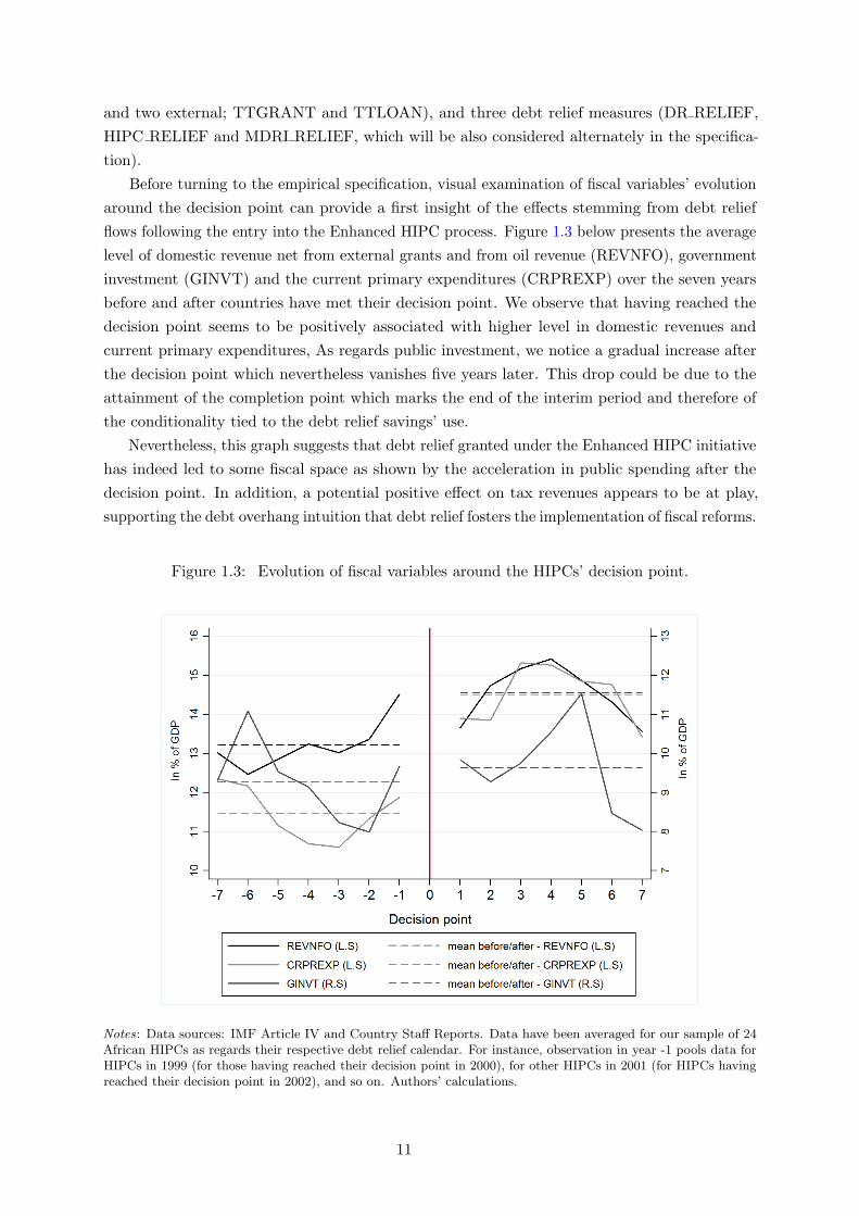
and two external; TTGRANT and TTLOAN), and three debt relief measures (DR RELIEF,

HIPC RELIEF and MDRI RELIEF, which will be also considered alternately in the specifica-

tion).

Before turning to the empirical specification, visual examination of fiscal variables’ evolution

around the decision point can provide a first insight of the effects stemming from debt relief

flows following the entry into the Enhanced HIPC process. Figure 1.3 below presents the average

level of domestic revenue net from external grants and from oil revenue (REVNFO), government

investment (GINVT) and the current primary expenditures (CRPREXP) over the seven years

before and after countries have met their decision point. We observe that having reached the

decision point seems to be positively associated with higher level in domestic revenues and

current primary expenditures, As regards public investment, we notice a gradual increase after

the decision point which nevertheless vanishes five years later. This drop could be due to the

attainment of the completion point which marks the end of the interim period and therefore of

the conditionality tied to the debt relief savings’ use.

Nevertheless, this graph suggests that debt relief granted under the Enhanced HIPC initiative

has indeed led to some fiscal space as shown by the acceleration in public spending after the

decision point. In addition, a potential positive effect on tax revenues appears to be at play,

supporting the debt overhang intuition that debt relief fosters the implementation of fiscal reforms.

Figure 1.3: Evolution of fiscal variables around the HIPCs’ decision point.

Notes: Data sources: IMF Article IV and Country Staff Reports. Data have been averaged for our sample of 24African HIPCs as regards their respective debt relief calendar. For instance, observation in year -1 pools data forHIPCs in 1999 (for those having reached their decision point in 2000), for other HIPCs in 2001 (for HIPCs havingreached their decision point in 2002), and so on. Authors’ calculations.

11

1.3.3 Empirical framework: dealing with heterogeneity

As argued above, we consider the vector autoregressive approach (VAR) as the most suited

specification to observe how budgetary variables react to debt relief provision. Indeed, Heller

(1975) built his fiscal response model as a set of structural equations within which budgetary

variables are successively the dependent and the explanatory variable. Therefore, in keeping

with the theoretical fiscal response model of Heller (1975), the VAR specification represents

an appropriate method for investigating empirically of the nature of the interactions between

budgetary components.

Once the reduced form of the VAR specification is set, the VAR estimator basically applies

the classic OLS estimator on each equation of the system. However our VAR specification, has

to consider the panel dimension of our dataset. As we now work with several HIPC countries,

the OLS estimator cannot be used anymore. If used, OLS estimators will be definitively biased

because of potential correlation between explanatory variables and the error term, since estimate

residuals will surely contain omitted but potentially important country-specific factors. Therefore

we decide to pool observations and include country and time fixed effects in our VAR specification

(now called “panel VAR”) in order to account for the sample heterogeneity and for potential

common trends that might occur on such long period of study. The use of the panel VAR

approach is also motivated by the possibility of observing an average effect of the debt relief

initiatives within our sample. However, it would be misleading to claim that HIPCs are perfectly

identical to justify the use of such methodology, but we reasonably think that these countries

present enough similar features to use a common specification.

As alternative methodology —necessitating longer time series— Juselius et al. (2014) test

the impact of aid on long term growth using one VAR/VECM model for each country of their

sample. Such method allows to get individual coefficients and to observe the effect of aid on

GDP growth for the considered country. However, two things lead us to believe that the panel

VAR approach is more suited to our research question.

First, Juselius et al. (2014) are able to run individual VAR models thanks to long time

series on aid data and GDP growth (more than 40 years). We do not have such temporal depth

which therefore prevents us to apply similar models. Second, their motivations for estimating

individual specifications is also justified by the heterogeneity of their sample which contains

thirty-six sub-Saharan African countries exposing really different income level (Botswana, Gabon,

DRC and Somalia) and contrasting access to external financing. However, in our case, we argue

that our sample of 24 African HIPCs is much more homogenous since HIPCs were all classified

as low-income country (LIC) by the World Bank and were all IDA eligible (only, not blend8)

prior the Enhanced HIPC initiative.

Lastly, and as explained in Lof et al. (2015), another argument in favor of the panel VAR

methodology is that pooled panel VAR allows to significantly increase the number of observations

since instead of estimating individual VAR with country-level observations (for one country), we

are now able to run one VAR with many observations (over several countries). Our empirical

specification therefore takes the following form:

8The ‘blend’ label refers to countries which can either borrow from the IDA or the IBRD.

12

ri,t

vi,t

hi,t

Xi,t

=

c0r

c0v

c0hc0X

+

2∑

j=1

αrr,j αv

r,j αhr,j AX

r,j

αrv,j αv

v,j αhv,j AX

v,j

αrh,j αv

h,j αhh,j AX

h,j

αrX,j αv

X,j αhX,j AX

X,j

×

ri,t−j

vi,t−j

hi,t−j

Xi,t−j

+ τt + δi +

ǫri,tǫvi,tǫhi,tǫXi,t

(1.1)

where ri,t denotes the total domestic revenue for country i in year t, vi,t the government investment

for country i in year t, and hi,t the current primary expenditures for country i in year t. Xi,t is

vector that collects financing and debt relief variables. More specifically, we have X′

i,t = [fi,t; li,t;

gi,t; di,t], where fi,t is domestic financing for country i in year t, li,t represents loans for country

i in year t, gi,t denotes grants (net from debt relief grants) for country i in year t, and lastly

di,t is our variable of interest which corresponds to debt service savings derived from debt relief

for country i in year t, but can be a vector of two variables when disaggregated (d′

i,t =[hipci,t;

mdrii,t]). The number of lags in our VAR system is represented by j and is equal to 2 (according

to Akaike and Schwarz criterion). αj are all VAR parameters to be estimated for each equation

of our system (Aj being the vector of VAR parameters for the rest of variables). c0 is a constant

for each equation (c0X being the constant vector for the remaining variables of the system). δi

represents N-1 country fixed effects in each equation and τt represents T-1 time fixed effects in

each equation of the system. ǫri,t, ǫvi,t and ǫhi,t are classic error terms and ǫXi,t a vector of the error

terms of our set of financing and debt relief variables.

From our panel VAR estimates, we will only report results for three equations out of seven

(or eight when debt relief variable is disaggregated). These are the ones that show the effect

of debt relief on total domestic revenue (and alternately on revenue net from oil receipts), on

government investment and on current primary expenditures. More in particular, we report

results for the three following equations:

ri,t = c0r+δi+τt+2

∑

j=1

αrr,jri,t−j+

2∑

j=1

αvr,jvi,t−j+

2∑

j=1

αhr,jhi,t−j+

2∑

j=1

AX−1

r,j X−1,i,t−j+2

∑

j=1

αdr,jdi,t−j+ǫri,t

vi,t = c0v+δi+τt+2

∑

j=1

αrv,jri,t−j+

2∑

j=1

αvv,jvi,t−j+

2∑

j=1

αhv,jhi,t−j+

2∑

j=1

AX−1

v,j X−1,i,t−j+2

∑

j=1

αdv,jdi,t−j+ǫvi,t

hi,t = c0h+δi+τt+

2∑

j=1

αrh,jri,t−j+

2∑

j=1

αvh,jvi,t−j+

2∑

j=1

αhh,jhi,t−j+

2∑

j=1

AX−1

h,j X−1,i,t−j+

2∑

j=1

αdh,jdi,t−j+ǫhi,t

Another interesting feature of our empirical specification (related to the VAR approach) is

the ability to compute impulse response functions (IRFs) using the Sims’ approach popularized

in 1980 and which requires Cholesky decomposition to orthogonalize the shocks. IRFs represent

graphically how a budgetary variable reacts (holding everything else constant) over the short- and

the medium-term to a shock on an explanatory variable (such as debt relief flows for instance).

The use of IRFs thus provides additional information on the fiscal response’ length to debt relief

as well as information about the validity of our model since convergence in IRFs attests the

13

stability of the VAR model. Lastly, when using disaggregated measures of debt relief, the risk

that the model becomes over-parametrized increases, which is why, as a robustness check, we

also estimate our panel VAR with an aggregated measure of aid (loans and grants considered as

a sole aid flow).

1.4 Results, discussion and further analysis

In this section, we present the results of our panel vector autoregressive model. We only

report results for three equations out of the system of seven (eight in the case of disaggregated

debt relief) in the interest of space. We first focus on government investment since it is often

thought to be a particular sign of structural investment in social services, as favored by donors.

This type of government expenditure is also assumed to have a positive impact on future growth

as compared with current primary expenditures (that we also review). We then investigate the

effect of debt relief on future tax collection. This is because, as debt relief is not sustainable in

itself, the fiscal space created by debt relief can only be preserved in the future if debt relief also

leads to improve domestic revenue mobilization. Lastly, following the fiscal space predictions,

we try to go further by differentiating the debt relief impact over two sub-samples, the HIPCs

defined as “bad payers” and those considered as “good payers”.

1.4.1 Dynamic fiscal effects of debt relief on government investment and current primary

expenditures

Table 1.2 below shows results derived from the public investment and current primary

expenditures equations as estimated by the panel VAR model. Columns I and III report results

for aggregate debt relief effects on government investment using alternately total domestic

revenue and revenue net from oil. Columns II and IV present results for disaggregated debt relief

impacts on public investment using also the two measures of domestic revenue. Government

investment seems to be persistent, with an increase in the past period being associated with an

increase in the future. For the aid variables, as we might expect, past increases in loans seem to

have important effect. Indeed, government investment in developing countries and especially

in sub-Saharan African countries is mostly externally financed. This financing mainly occurs

through concessional borrowing from international financial institutions since these countries

are excluded from international financial markets. For total grants, the results suggest a strong

positive effect in the following year, although this effect seems to be slightly offset the year after.

As regards our variables of interest, we find a statistically significant effect of aggregate

debt relief on public investment. According to our results, the debt relief impact occurs after

one year and is around 0.35 suggesting that an increase in debt service savings from debt relief

initiative by 10% in T is associated with a 3.5% increase in public investment in T+1. More

interesting, when differentiating debt relief between the two initiatives, it appears that the bulk

of this effect is due to the Enhanced HIPC initiative. In particular, an increase in debt service

savings of 10% under the Enhanced HIPC initiative in the previous year is associated with an

increase of around 4.6% in public investment as a share of GDP the year after. The effect is

14

similar and even higher in magnitude than those of total grants and total loans.9 The absence

of result for debt service savings from the MDRI however suggests that the fiscal space created

by MDRI does not result in investment increase. This may be explained by the fact that, unlike

HIPC debt reduction, MDRI is much less able to let the conditionality effect work due to its

one-off nature. The Enhanced HIPC initiative was indeed accompanied by a close follow-up of

expenditures financed by money freed by debt relief (which had to be transferred to a special

banking account), that aimed at promoting public investment, mostly in social sectors, over the

short- and medium-term as its impulse response attests in Figure 1.A1 in the Appendix (p.26).10

Achieving the completion point of the HIPC initiative was indeed subject to a precise set of

conditions. Conversely, after the completion point, debt relief under HIPC becomes irrevocable

and MDRI is granted without further conditions.

The debt relief impacts on current primary expenditures seem to support this explanation.

Indeed, although columns V and VII from Table 1.2 expose an absence of effect from debt

relief granted as a whole, results with disaggregated debt relief expose a strong and positive

effect of debt service savings from the MDRI on current primary expenditures. These results

provide therefore empirical support to what we argue in introduction and in the Section 1.2.3.

Debt relief under MDRI seems to significantly free-up resources that would have been otherwise

spent on debt service payments (since the post-Enhanced HIPC initiative debt should have been

sustainable). Moreover, looking at coefficients magnitude, results could suggest that HIPCs’

governments are close to the most extreme picture we depict in Section 1.2.4 where they are

considered as both credit-constrained and highly impatient (which is, according to us, the most

likely case out of the four presented). In addition, the MDRI savings allocation toward current

primary expenditures rather than capital spending also appears quite intuitive if one look at the

design of the debt relief initiatives. Since, under the HIPC initiative, government was biased to

target money freed up by debt relief predominantly to public investment, positive impacts of

debt relief flows from the MDRI could simply reflect the combination of fiscal space with the

absence of conditionality which leads beneficiary governments to go back to old policies where

current expenditures were preferred to structural ones.

However, we could also imagine a more positive picture where the increase in current primary

expenditures stemming from the MDRI will aim at financing running costs associated with the

initial investment undertaken thanks to debt relief granted under the Enhanced HIPC initiative.

The increase in current primary expenditures would therefore suggest that investment stemming

from debt relief are not doomed to transform in “white elephants”, but are intended to be

perennial. Note that replacing loans and grants by the aggregate measure of aid flows (AID)

does not alter the results (see Table 1.A2 in the Appendix, p.29).

9Moreover, we do not find significant crowding-out effects of the debt relief initiatives on other aid flows (totalgrants and loans) which confirms the realization of a net fiscal space induced by these initiatives.

10Note that convergence in the IRFs attests the absence of unit root in our panel VAR (stable necessarycondition). IRF are only interpreted for significant results.

15

Table 1.2: Debt relief impacts on public spending.

(I) (II) (III) (IV) (V) (VI) (VII) (VIII)

Dep. var.: GINVT CRPREXP

TTREV t-1 0.069 0.068 0.294*** 0.298***(0.067) (0.067) (0.043) (0.043)

TTREV t-2 0.068 0.064 -0.040 -0.037(0.069) (0.069) (0.044) (0.044)

REVNFO t-1 -0.050 -0.049 0.357*** 0.368***(0.081) (0.081) (0.053) (0.053)

REVNFO t-2 0.113 0.105 -0.214*** -0.215***(0.081) (0.081) (0.053) (0.052)

CRPREXP t-1 0.012 0.013 0.069 0.070 0.403*** 0.394*** 0.449*** 0.439***(0.066) (0.066) (0.065) (0.065) (0.042) (0.042) (0.042) (0.042)

CRPREXP t-2 -0.027 -0.024 -0.030 -0.027 0.045 0.047 0.116*** 0.120***(0.063) (0.063) (0.063) (0.063) (0.041) (0.040) (0.041) (0.041)

GINVT t-1 0.174*** 0.171*** 0.193*** 0.190*** -0.076*** -0.075*** -0.045 -0.044(0.044) (0.044) (0.043) (0.043) (0.028) (0.028) (0.028) (0.028)

GINVT t-2 0.061 0.065 0.075* 0.079* 0.030 0.030 0.056** 0.057**(0.043) (0.044) (0.042) (0.042) (0.028) (0.028) (0.028) (0.027)

DFINA t-1 0.009 0.009 0.006 0.006 0.016 0.016 0.007 0.007(0.018) (0.018) (0.018) (0.018) (0.012) (0.011) (0.012) (0.012)

DFINA t-2 -0.025 -0.025 -0.029 -0.029 -0.008 -0.008 -0.008 -0.008(0.018) (0.018) (0.018) (0.018) (0.011) (0.011) (0.012) (0.011)

TTGRANT t-1 0.226*** 0.218*** 0.215*** 0.208*** 0.011 0.013 -0.047 -0.048(0.072) (0.072) (0.072) (0.072) (0.046) (0.046) (0.047) (0.046)

TTGRANT t-2 -0.134* -0.138* -0.154** -0.158** 0.082* 0.092** 0.058 0.067(0.071) (0.071) (0.070) (0.070) (0.046) (0.045) (0.046) (0.045)

TTLOAN t-1 0.142** 0.145** 0.142** 0.146** 0.104*** 0.100** 0.106*** 0.103***(0.061) (0.061) (0.061) (0.061) (0.039) (0.039) (0.040) (0.040)

TTLOAN t-2 0.182*** 0.186*** 0.179*** 0.183*** -0.048 -0.052 -0.049 -0.053(0.060) (0.060) (0.060) (0.060) (0.039) (0.039) (0.039) (0.039)

DEBT RELIEF t-1 0.353** 0.351* -0.095 -0.112(0.180) (0.180) (0.116) (0.117)

DEBT RELIEF t-2 0.022 0.003 0.160 0.147(0.176) (0.176) (0.113) (0.114)

HIPC RELIEF t-1 0.469** 0.466** -0.086 -0.077(0.199) (0.200) (0.128) (0.129)

HIPC RELIEF t-2 0.003 -0.004 0.018 -0.011(0.197) (0.198) (0.126) (0.128)

MDRI RELIEF t-1 -0.357 -0.341 -0.225 -0.414(0.572) (0.574) (0.367) (0.371)

MDRI RELIEF t-2 0.324 0.257 0.875** 0.979***(0.559) (0.562) (0.359) (0.363)

Constant -0.677 -0.186 -0.084 0.457 0.920 0.335 1.144 0.574(1.684) (1.731) (1.800) (1.848) (1.085) (1.109) (1.168) (1.194)

Country/time FE Yes Yes Yes Yes Yes Yes Yes YesR-Squared 0.665 0.666 0.664 0.665 0.673 0.677 0.667 0.671

χ2 test (p-value) 0.000 0.000 0.000 0.000 0.000 0.000 0.000 0.000Observations 637 637 637 637 637 637 637 637

Notes: The table reports VAR equations only for government investment and current primary expenditures. Coefficients areexposed with, in brackets, their associated standard errors. t-1 and t-2 reflects variables with respectively one and two periodlags. Country and time fixed effects (FE) are included as exogenous block. ***, ** and * denote significance at 10%, 5% and 1%.

16

1.4.2 Dynamic fiscal effects of debt relief on tax mobilization

Table 1.3 presents the results from the equations of our panel VAR that model the effect

of different fiscal variables on total domestic revenue. We expose results for our two revenue

variables (total domestic revenue and revenue net from natural resources receipts) and using

alternately aggregate and disaggregated debt relief variables. As for public investment and

current primary expenditures equations, domestic revenue seem to be persistent over time, with

an increase in the past period also being associated with a current increase.

Columns I—IV expose results for our broader measure of domestic revenue. Column I and II

show a positive debt relief impact on the total domestic revenue. When we differentiate between

HIPC and MDRI, we find that this positive impact seems to be essentially due to debt relief

granted under the MDRI.

Nevertheless, as explained in the previous section, there is a risk that positive correlation

between debt relief and total domestic revenue might be due to the spike in oil prices that

occurred in the mid-2000s. Some countries of our sample rely significantly on oil-related revenue

(Chad, Cameroon) and received debt relief around the spame period. In order to identify the

debt relief effects on genuine domestic effort in terms of tax collection, it would be therefore

preferable to look at the effects on revenue net from oil and other natural resources receipts.

Columns V-VI in Table 1.3 thus report estimates where revenue net from natural resources

receipts is the dependent variable. Once again, tax revenue are positively associated with their

past values. Moreover, debt service savings from debt relief taken as a whole is still positively

and significantly associated with tax revenue. However, conversely to results in column (II), it

now seems more difficult to identify the initiative responsible for such effect.

Lastly, since resource rich countries have a larger share of their revenue derived from natural

resources related activites which can impact both revenue and the GDP, we also run panel

VAR models excluding three countries of our sample that have (on average and over the period

considered) at least 25% of their domestic revenue stemming from the natural resources sector.

This leads us to remove from the sample Cameroon (with 32% of its domestic revenue derived

from the oil sector), Chad (with 25% of total domestic revenue as oil revenue) and Guinea (with

36% of revenue related to the mining sector). Columns (III), (IV), (VII) and (VIII) expose the

results. Excluding these resource-rich countries does not distort the results. Debt service savings

from debt relief are significant at the 5% level with the aggregate measure of domestic revenue

and significant at almost 5% (the associated p-value is equal to 0.051) with the revenue net from

natural resources receipts.Using this last measure, we also notice that as before, the effect from

the overall debt relief seems to be driven by the MDRI. As a result, and although not obvious in

the impulse response function (see Figure 1.A1 in the Appendix, p.26), it is likely that debt relief

under the MDRI is the key driver of the positive reaction of domestic revenues to debt relief. So

to conclude, if we consider debt relief as a whole (which is more intuitive when looking at the

impact on domestic revenue), results suggest that an increase in debt service savings of 10% in

the previous year is associated with an increase between 1.5 and 1.9% in domestic revenue (net

from natural resources receipts and grants) as a share of GDP two years after.

17

Table 1.3: Debt relief impacts on total domestic revenues (gross and net from oil).

(I) (II) (III) (IV) (V) (VI) (VII) (VIII)

Dep. var.: TTREV REV NFO

TTREV t-1 0.663*** 0.664*** 0.516*** 0.516***(0.043) (0.043) (0.045) (0.045)

TTREV t-2 0.007 0.006 -0.024 -0.022(0.044) (0.044) (0.043) (0.043)

REVNFO t-1 0.588*** 0.590*** 0.578*** 0.579***(0.042) (0.042) (0.045) (0.045)

REVNFO t-2 -0.043 -0.048 -0.019 -0.020(0.042) (0.042) (0.046) (0.046)

CRPREXP t-1 -0.017 -0.021 -0.009 -0.012 -0.029 -0.030 -0.037 -0.039(0.042) (0.042) (0.038) (0.038) (0.034) (0.034) (0.037) (0.037)

CRPREXP t-2 0.007 0.010 0.016 0.015 0.026 0.028 0.024 0.025(0.040) (0.040) (0.036) (0.036) (0.033) (0.033) (0.036) (0.036)

GINVT t-1 -0.018 -0.019 -0.021 -0.021 -0.004 -0.005 -0.009 -0.010(0.028) (0.028) (0.025) (0.025) (0.022) (0.022) (0.024) (0.024)

GINVT t-2 0.004 0.007 -0.004 -0.004 -0.000 0.002 -0.006 -0.005(0.028) (0.028) (0.025) (0.025) (0.022) (0.022) (0.024) (0.024)

DFINA t-1 -0.004 -0.004 -0.010 -0.010 -0.020** -0.019** -0.018* -0.018*(0.011) (0.011) (0.010) (0.010) (0.009) (0.009) (0.010) (0.010)

DFINA t-2 -0.008 -0.008 -0.012 -0.012 -0.006 -0.006 -0.004 -0.004(0.011) (0.011) (0.010) (0.010) (0.009) (0.009) (0.010) (0.010)

TTGRANT t-1 0.002 -0.003 0.060 0.062 0.044 0.040 0.066 0.063(0.046) (0.046) (0.049) (0.049) (0.037) (0.037) (0.048) (0.049)

TTGRANT t-2 0.021 0.023 0.015 0.019 0.020 0.019 0.012 0.014(0.045) (0.045) (0.048) (0.048) (0.037) (0.037) (0.047) (0.047)

TTLOAN t-1 0.052 0.053 0.047 0.047 0.038 0.039 0.040 0.041(0.039) (0.039) (0.035) (0.035) (0.032) (0.032) (0.035) (0.035)

TTLOAN t-2 -0.015 -0.014 -0.004 -0.007 -0.017 -0.015 -0.021 -0.021(0.038) (0.038) (0.035) (0.035) (0.031) (0.031) (0.034) (0.034)

DEBT RELIEF t-1 -0.064 0.039 -0.033 -0.001(0.115) (0.102) (0.094) (0.100)

DEBT RELIEF t-2 0.187* 0.215** 0.152* 0.192*(0.113) (0.100) (0.092) (0.098)

HIPC RELIEF t-1 0.013 0.046 0.032 0.046(0.127) (0.111) (0.104) (0.109)

HIPC RELIEF t-2 0.106 0.160 0.123 0.139(0.126) (0.110) (0.103) (0.108)

MDRI RELIEF t-1 -0.571 -0.055 -0.436 -0.357(0.366) (0.333) (0.299) (0.328)

MDRI RELIEF t-2 0.724** 0.535 0.414 0.594*(0.358) (0.328) (0.293) (0.323)

Constant 2.375** 2.397** 5.324*** 5.126*** 5.372*** 5.561*** 5.964*** 5.939***(1.077) (1.107) (1.015) (1.032) (0.938) (0.963) (0.994) (1.018)

Country/time FE Yes Yes Yes Yes Yes Yes Yes YesResource-rich countries Yes Yes No No Yes Yes No No

R-Squared 0.740 0.741 0.765 0.765 0.795 0.795 0.773 0.774χ2 test (p-value) 0.000 0.000 0.000 0.000 0.000 0.000 0.000 0.000

Observations 637 637 588 588 637 637 558 558

Notes: The table reports VAR equations only for total domestic revenue and total domestic revenue net from oil. Coefficients areexposed with, in brackets, their associated standard errors. t-1 and t-2 reflects variables with respectively one and two periodlags. Country and time fixed effects (FE) are included as exogenous block. ***, ** and * denote significance at 10%, 5% and 1%.

18

1.4.3 Bad payers versus good payers: does being a good payer increase relative impact?

As exposed above, our measure of debt relief might be subject to the criticism that, in the

absence of debt relief, debt would not have been serviced (at least fully). In such a case, cash flow

gains from debt relief would be closed to zero. In order to consider that debt relief’s benefits are

not as high for bad payers as for good payers, we then split our sample in two sub-samples; the

bad and good payers. This distinction is based on the share of long-term debt arrears of HIPCs

countries the year before the HIPC initiative was made public, so in 1995. We decided to focus

on 1995 because once the initiative made public (in 1996), some HIPCs would have been tempted

to not reimburse their debt and accumulate arrears in order to breach the insolvency threshold

and get debt relief from international financial institutions. This differentiation leads the bad

payers’ sub-sample to include eleven countries for which the share of long-term debt arrears

over the external debt was higher than 10% in 1995. The good payers’ sub-sample contains the

remaining thirteen countries for which this share was below 10% the same year.

However this proxy for the government’s willingness to pay should be taken cautiously since

Table 1.A3 (p.30 in the Appendix) exposes level of arrears that are relatively low as compared

with what one would have expected. Explanations for such low stock of arrears can be found

in the ever greening practice from international financial institutions which, over the 1990s,

continued to provide loans (Geginat and Kraay, 2012) (and even grants11) to these countries

in order to make them able to repay the old ones. Therefore, since the stock of arrears does

not take this potential defensive lending into account, one could consider that our proxy reflects

more potential disagreements between governments and IFIs in debt repaying procedures rather

than the exact measure of willingness to pay. That said, to our knowledge, building a proxy for

the state’s willingness to pay that accounts for defensive lending would require a loan-by-loan

approach which, as regards sub-Saharan African HIPCs, seems quite unrealistic given the data

availability and the blurred boundary between what could be considered as defensive lending

and what cannot. That is why we finally decided to keep the stock of arrears as our proxy for

the government’s willingness to pay, although we acknowledge this proxy has some limits.

Table 1.4 shows the results on public spending for bad payers only. The impact of debt relief

on capital expenditures is positive and significant at the 10% level though we do not know which

program (HIPC or MDRI) fuels this effect. But the magnitude of the debt relief coefficient now

ranges between 0.30 and 0.26 which is less than when we considered the entire sample. This

is seems consistent with the fiscal space prediction suggesting that fiscal space created by the

Enhanced HIPC initiative should be less important for countries which were not fully servicing

their debt prior cancellations. Conversely, the impact of debt relief on public investment for

countries that did honor their debt service is quite interesting. Table 1.5 indeed exposes a

positive and significant (though only at the 10% level) impact for HIPC debt relief that is almost

three times larger than the one found for bad payers and for the whole sample, although maybe

less perennial according to the IRFs.12 This also supports the fiscal space intuition arguing

that, conversely to the situation for bad payers, countries which were previously repaying their

11Cf. Marchesi and Missale (2013).12See Figure 1.A2 (p.27) and 1.A3 (p.27) the Appendix. Convergence in IRFs for the two sub-samples also

verifies the stable condition of the corresponding panel VAR.

19

debt should have benefited from a significant fiscal space when international creditors decided

to cancel their debt down to sustainable levels. Broadly speaking, it basically means that debt

relief has been more effective in terms of public investment for countries which were meeting

their liabilities prior to the HIPC initiative (and that maybe also had better institutions).

Furthermore, columns (V) and (VII) show that this larger fiscal space perceived by good

payers also helped to increase current primary expenditures two years after the debt relief

provision (and according to column (VI) after debt relief provided under the Enhanced HIPC

initiative). This is quite consistent with Table 1.2 (p.16) findings, where increase in current

primary expenditures due to debt relief was probably intended to finance running costs associ-

ated with investment initially undertaken thanks to the first wave of resources freed up by the

Enhanced HIPC initiative (in the case of good payers).

Lastly, looking at Table 1.6 which presents results for good and bad payers on domestic

revenue, we find that debt relief provided under the Enhanced HIPC initiative has had a positive

and significant impact on revenue net from natural resources for good payers.

Following the debt overhang theory developed by Krugman (1988), such fiscal reaction might

be motivated by the fact that, before benefiting from debt relief, external creditors were putting

substantial pressure on highly indebted countries’ governments as regards debt repayments.

Therefore, the additional tax receipts that indebted countries might have collected would have

been immediately grabbed by creditors. Then, it would have been more interesting for those

indebted countries not to engage in such tax collection effort, not reimburse debt service and to

await debt relief before implementing such policy which could then favor directly the domestic

public administration and not be “expropriated” by external creditors.

In addition other conditionality effects might be at play since eligible criteria prior to the

Enhanced HIPC initiative also required to implement macroeconomic reforms such as tax base

improvements and better tax collection. The reason for larger impacts on domestic revenue

for good payers could be thus explained by the fact that good payers probably have better

institutions and therefore strongly stuck to IMF and IDA recommendations in order to get

debt relief, which in fine might have helped to improve domestic revenue mobilization. In

contrast with the domestic revenue response for bad payers, we see that the magnitude of

the debt relief effect on domestic revenue is less important and less robust for good payers,

which does not go in favor of this conditionality argument, even though one can be dubious

about the real impact of debt relief on taxation for bad payers since the coefficient becomes

not statistically significant when we use our preferred measure of domestic revenue (column (VII)).

20

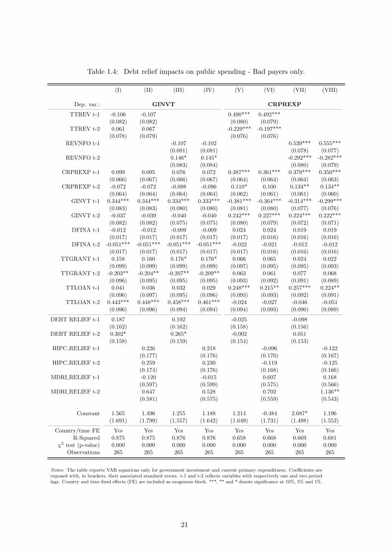
Table 1.4: Debt relief impacts on public spending - Bad payers only.

(I) (II) (III) (IV) (V) (VI) (VII) (VIII)

Dep. var.: GINVT CRPREXP

TTREV t-1 -0.106 -0.107 0.490*** 0.492***(0.082) (0.082) (0.080) (0.079)

TTREV t-2 0.061 0.067 -0.229*** -0.197***(0.078) (0.079) (0.076) (0.076)

REVNFO t-1 -0.107 -0.102 0.539*** 0.555***(0.081) (0.081) (0.078) (0.077)

REVNFO t-2 0.146* 0.145* -0.292*** -0.282***(0.083) (0.084) (0.080) (0.079)

CRPREXP t-1 0.099 0.095 0.076 0.072 0.387*** 0.361*** 0.379*** 0.350***(0.066) (0.067) (0.066) (0.067) (0.064) (0.064) (0.064) (0.063)

CRPREXP t-2 -0.072 -0.072 -0.098 -0.096 0.110* 0.100 0.134** 0.134**(0.064) (0.064) (0.064) (0.064) (0.062) (0.061) (0.061) (0.060)

GINVT t-1 0.344*** 0.344*** 0.334*** 0.333*** -0.381*** -0.364*** -0.314*** -0.299***(0.083) (0.083) (0.080) (0.080) (0.081) (0.080) (0.077) (0.076)

GINVT t-2 -0.037 -0.039 -0.040 -0.040 0.242*** 0.227*** 0.224*** 0.222***(0.082) (0.082) (0.075) (0.075) (0.080) (0.079) (0.072) (0.071)

DFINA t-1 -0.012 -0.012 -0.009 -0.009 0.024 0.024 0.019 0.019(0.017) (0.017) (0.017) (0.017) (0.017) (0.016) (0.016) (0.016)

DFINA t-2 -0.051*** -0.051*** -0.051*** -0.051*** -0.022 -0.021 -0.012 -0.012(0.017) (0.017) (0.017) (0.017) (0.017) (0.016) (0.016) (0.016)

TTGRANT t-1 0.158 0.160 0.176* 0.176* 0.066 0.065 0.024 0.022(0.099) (0.099) (0.099) (0.099) (0.097) (0.095) (0.095) (0.093)

TTGRANT t-2 -0.203** -0.204** -0.207** -0.209** 0.063 0.061 0.077 0.068(0.096) (0.095) (0.095) (0.095) (0.093) (0.092) (0.091) (0.089)

TTLOAN t-1 0.041 0.036 0.032 0.029 0.248*** 0.215** 0.257*** 0.224**(0.096) (0.097) (0.095) (0.096) (0.093) (0.093) (0.092) (0.091)

TTLOAN t-2 0.443*** 0.448*** 0.458*** 0.461*** -0.024 -0.027 -0.046 -0.051(0.096) (0.096) (0.094) (0.094) (0.094) (0.093) (0.090) (0.089)

DEBT RELIEF t-1 0.187 0.192 -0.025 -0.098(0.162) (0.162) (0.158) (0.156)

DEBT RELIEF t-2 0.302* 0.265* -0.002 0.051(0.158) (0.159) (0.154) (0.153)

HIPC RELIEF t-1 0.226 0.218 -0.096 -0.122(0.177) (0.176) (0.170) (0.167)

HIPC RELIEF t-2 0.259 0.230 -0.119 -0.125(0.174) (0.176) (0.168) (0.166)

MDRI RELIEF t-1 -0.120 -0.015 0.607 0.168(0.597) (0.599) (0.575) (0.566)

MDRI RELIEF t-2 0.647 0.528 0.702 1.136**(0.581) (0.575) (0.559) (0.543)

Constant 1.565 1.496 1.255 1.188 1.214 -0.484 2.687* 1.196(1.691) (1.799) (1.557) (1.642) (1.649) (1.731) (1.498) (1.552)

Country/time FE Yes Yes Yes Yes Yes Yes Yes YesR-Squared 0.875 0.875 0.876 0.876 0.658 0.668 0.669 0.681

χ2 test (p-value) 0.000 0.000 0.000 0.000 0.000 0.000 0.000 0.000Observations 265 265 265 265 265 265 265 265

Notes: The table reports VAR equations only for government investment and current primary expenditures. Coefficients areexposed with, in brackets, their associated standard errors. t-1 and t-2 reflects variables with respectively one and two periodlags. Country and time fixed effects (FE) are included as exogenous block. ***, ** and * denote significance at 10%, 5% and 1%.

21

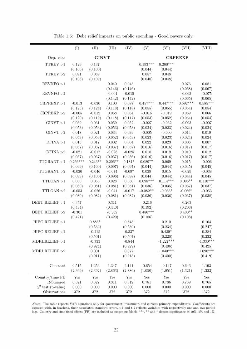
Table 1.5: Debt relief impacts on public spending - Good payers only.

(I) (II) (III) (IV) (V) (VI) (VII) (VIII)

Dep. var.: GINVT CRPREXP

TTREV t-1 0.129 0.137 0.193*** 0.200***(0.100) (0.100) (0.044) (0.044)

TTREV t-2 0.091 0.089 0.057 0.048(0.108) (0.109) (0.048) (0.048)

REVNFO t-1 0.040 0.045 0.076 0.081(0.146) (0.146) (0.068) (0.067)

REVNFO t-2 -0.004 -0.015 -0.063 -0.075(0.142) (0.142) (0.065) (0.065)

CRPREXP t-1 -0.013 -0.030 0.100 0.087 0.457*** 0.447*** 0.592*** 0.585***(0.125) (0.124) (0.118) (0.118) (0.055) (0.055) (0.054) (0.054)

CRPREXP t-2 -0.005 -0.012 0.068 0.064 -0.016 -0.019 0.069 0.066(0.120) (0.119) (0.118) (0.117) (0.053) (0.052) (0.054) (0.054)

GINVT t-1 0.039 0.031 0.059 0.052 -0.027 -0.032 -0.003 -0.007(0.053) (0.053) (0.053) (0.053) (0.024) (0.023) (0.024) (0.024)

GINVT t-2 0.018 0.021 0.034 0.039 -0.005 -0.000 0.014 0.019(0.053) (0.053) (0.052) (0.053) (0.023) (0.023) (0.024) (0.024)

DFINA t-1 0.015 0.017 0.002 0.004 0.022 0.023 0.006 0.007(0.037) (0.037) (0.037) (0.037) (0.016) (0.016) (0.017) (0.017)

DFINA t-2 -0.021 -0.017 -0.028 -0.025 0.018 0.019 0.010 0.012(0.037) (0.037) (0.037) (0.036) (0.016) (0.016) (0.017) (0.017)

TTGRANT t-1 0.266*** 0.243** 0.206** 0.181* 0.089** 0.069 0.015 -0.006(0.099) (0.100) (0.097) (0.097) (0.044) (0.044) (0.045) (0.045)

TTGRANT t-2 -0.020 -0.046 -0.074 -0.097 0.029 0.015 -0.029 -0.038(0.099) (0.100) (0.096) (0.098) (0.044) (0.044) (0.044) (0.045)

TTLOAN t-1 0.030 0.053 0.028 0.050 0.098*** 0.114*** 0.096** 0.110***(0.080) (0.081) (0.081) (0.081) (0.036) (0.035) (0.037) (0.037)

TTLOAN t-2 -0.053 -0.026 -0.041 -0.017 -0.082** -0.066* -0.066* -0.053(0.080) (0.082) (0.081) (0.082) (0.036) (0.036) (0.037) (0.038)

DEBT RELIEF t-1 0.357 0.311 -0.216 -0.263(0.434) (0.440) (0.192) (0.203)

DEBT RELIEF t-2 -0.301 -0.362 0.486*** 0.400**(0.421) (0.429) (0.186) (0.198)

HIPC RELIEF t-1 0.886* 0.843 0.210 0.164(0.532) (0.539) (0.234) (0.247)

HIPC RELIEF t-2 -0.215 -0.337 0.429* 0.284(0.501) (0.507) (0.220) (0.232)

MDRI RELIEF t-1 -0.733 -0.844 -1.227*** -1.330***(0.924) (0.929) (0.406) (0.425)

MDRI RELIEF t-2 0.001 0.077 1.040*** 1.090***(0.911) (0.915) (0.400) (0.419)

Constant 0.515 1.256 1.347 2.141 -0.654 -0.147 0.646 1.193(2.369) (2.392) (2.863) (2.886) (1.050) (1.051) (1.321) (1.322)

Country/time FE Yes Yes Yes Yes Yes Yes Yes YesR-Squared 0.321 0.327 0.311 0.312 0.781 0.786 0.759 0.765

χ2 test (p-value) 0.000 0.000 0.000 0.000 0.000 0.000 0.000 0.000Observations 372 372 372 372 372 372 372 372

Notes: The table reports VAR equations only for government investment and current primary expenditures. Coefficients areexposed with, in brackets, their associated standard errors. t-1 and t-2 reflects variables with respectively one and two periodlags. Country and time fixed effects (FE) are included as exogenous block. ***, ** and * denote significance at 10%, 5% and 1%.

22

Table 1.6: Debt relief impacts on domestic revenue - Good vs. Bad payers.

(I) (II) (III) (IV) (V) (VI) (VII) (VIII)

Good Payers only Bad Payers only

Dep. var.: TTREV REVNFO TTREV REVNFO

TTREV T-1 0.709*** 0.724*** 0.496*** 0.498***(0.056) (0.055) (0.068) (0.067)

TTREV T-2 0.048 0.020 -0.056 -0.047(0.061) (0.060) (0.064) (0.065)

REVNFO T-1 0.576*** 0.582*** 0.577*** 0.575***(0.053) (0.052) (0.068) (0.068)

REVNFO T-2 -0.050 -0.066 -0.038 -0.039(0.052) (0.051) (0.070) (0.070)

CRPREXP T-1 0.144** 0.140** 0.081* 0.075* -0.010 -0.017 -0.058 -0.055(0.070) (0.069) (0.043) (0.042) (0.055) (0.055) (0.055) (0.056)

CRPREXP T-2 -0.102 -0.101 -0.070 -0.072* 0.063 0.058 0.064 0.063(0.067) (0.066) (0.043) (0.042) (0.053) (0.053) (0.053) (0.053)

GINVT T-1 0.021 0.018 0.016 0.013 -0.111 -0.103 -0.044 -0.045(0.030) (0.029) (0.019) (0.019) (0.069) (0.069) (0.067) (0.067)

GINVT T-2 0.007 0.020 0.007 0.015 0.052 0.047 0.041 0.041(0.029) (0.029) (0.019) (0.019) (0.068) (0.067) (0.063) (0.063)

DFINA T-1 0.037* 0.038* 0.023* 0.024* -0.019 -0.019 -0.035** -0.035**(0.021) (0.020) (0.013) (0.013) (0.014) (0.014) (0.014) (0.014)

DFINA T-2 0.025 0.025 0.023* 0.024* -0.026* -0.025* -0.015 -0.015(0.020) (0.020) (0.013) (0.013) (0.014) (0.014) (0.014) (0.014)

TTGRANT T-1 -0.013 -0.046 0.054 0.032 0.083 0.081 0.060 0.060(0.055) (0.055) (0.035) (0.035) (0.082) (0.082) (0.083) (0.083)

TTGRANT T-2 -0.007 -0.010 -0.009 -0.011 0.025 0.024 0.026 0.027(0.055) (0.055) (0.035) (0.035) (0.079) (0.079) (0.079) (0.079)

TTLOAN T-1 0.102** 0.119*** 0.070** 0.083*** 0.068 0.058 0.047 0.050(0.045) (0.044) (0.029) (0.029) (0.079) (0.080) (0.080) (0.080)

TTLOAN T-2 -0.020 -0.013 0.005 0.013 -0.025 -0.032 -0.046 -0.046(0.045) (0.045) (0.029) (0.029) (0.080) (0.079) (0.078) (0.079)

DEBT RELIEF T-1 -0.193 0.014 0.076 0.017(0.243) (0.160) (0.135) (0.136)

DEBT RELIEF T-2 0.081 0.058 0.243* 0.145(0.235) (0.156) (0.131) (0.133)

HIPC RELIEF T-1 0.411 0.441** 0.005 0.013(0.293) (0.193) (0.146) (0.148)

HIPC RELIEF T-2 -0.313 -0.170 0.234 0.166(0.276) (0.182) (0.144) (0.147)

MDRI RELIEF T-1 -1.960*** -1.174*** 0.678 0.043(0.509) (0.333) (0.494) (0.501)

MDRI RELIEF T-2 1.643*** 1.028*** 0.211 0.000(0.502) (0.328) (0.480) (0.481)

Constant 0.398 0.894 4.857*** 5.331*** 3.900*** 3.198** 2.142* 2.274*(1.327) (1.318) (1.043) (1.034) (1.402) (1.486) (1.302) (1.373)

Country/time FE Yes Yes Yes Yes Yes Yes Yes YesR-Squared 0.791 0.800 0.859 0.865 0.732 0.735 0.763 0.764

χ2 test (p-value) 0.000 0.000 0.000 0.000 0.000 0.000 0.000 0.000Observations 372 372 372 372 265 265 265 265

Notes: The table reports VAR equations only for total domestic revenue and total domestic revenue net from oil.Coefficients are exposed with, in brackets, their associated standard errors. t-1 and t-2 reflects variables with respectivelyone and two period lags. Country and time fixed effects (FE) are included as exogenous block. ***, ** and * denotesignificance at 10%, 5% and 1%.

23

Conclusion

Over the last 20 years, debt relief has been added to the tools of development interventions

used by bilateral donors at the macro level as well as multilateral development organizations as

the World Bank, the International Monetary Fund, African Development Bank, and the Inter-

American Development Bank. As with other development interventions such as (concessional)

loans and grants, there is a substantial body of literature describing how, in theory, debt relief

could lead to growth and poverty reduction. Now that over USD 76 billion worth of debt relief

(in present value terms) has been given through HIPC and MDRI, the question emerges if these

benefits can also be established empirically.

In this paper, we use a standard Vector Auto Regressive fiscal response model. Unlike the

standard ”aid-growth” literature, these models explicitly acknowledge that aid is given primarily

to the government, and that any impact of aid on the economy will hence depend on government

behavior, in particular how fiscal decisions on taxation and expenditure are affected by aid

revenues (Franco-Rodriguez et al., 1998; Franco-Rodriguez, 2000). Throughout this study, we

focus on the fiscal response effects of debt relief as an alternative instrument of aid delivery on

three important fiscal variables. We make a distinction between HIPC and MDRI, as the logic

behind these two debt relief initiatives is quite different. In addition we also differentiate the

fiscal response of debt relief according to the credit history of beneficiary countries.

Using appropriate panel vector autoregressive models, we do find positive and substantial

effects for aggregate debt relief on public investment. Moreover, when we differentiate debt relief

between HIPC and MDRI, we observe that debt relief under HIPC fosters capital expenditures

with a stronger effect for countries that were repaying their debt, providing empirical support

to the fiscal space predictions. According to our result, debt relief under the MDRI also favors

fiscal space creation which seems more targeted to current primary expenditures than capital

spending. We feel this may be because HIPC came with a close follow-up of public spending

financed by debt relief and strong conditionality at completion point. Threats of not meeting

donors’ expectations leading to less debt reduction in the future were credible. Debt relief after

completion point and MDRI is different, as it consists in irrevocable debt relief granted to HIPCs’

governments. Nevertheless, MDRI impacts on current primary expenses can be either considered

as a “back to normal” behavior from government or an increasing financial support (operating

costs) for public investment achieved through the HIPC initiative.

Lastly, although this study shows that debt relief generates fiscal space, one might wonder

whether this fiscal space is expected to be perennial and serve economic growth in the short- and

medium-run. Hence, for fiscal space created by debt relief to be sustainable and effective, other

types of fiscal revenue should respond positively as well (Addison, 2008). We find that aggregate

debt relief has this sort of crowding in effect on domestic revenue mobilization, although we do

not know exactly through which initiative this effect might be fueled. Furthermore, the response

of tax revenue following the decomposition between good and bad payers brings additional

support to the debt overhang theory and also emphasizes potential conditionality effects related

to eligible criteria which would deserve to be investigated in depth.

24

In overall, it seems that the Enhanced HIPC initiative had led to significant fiscal space

that fostered public investment in the benefiting countries. However, the lack of conditionality

attached to MDRI did not result in similar increase in capital expenditures, although positive

effects on current primary expenditures might be seen as supplementary financing for running

costs associated with investment undertaken under the Enhanced HIPC. Moreover, a robust

positive effect of MDRI on domestic revenue mobilization is lacking, casting doubt about the

sustainability of the fiscal space created by these debt relief initiatives.

25

Appendix

Figure 1.A1: Impulse response function to debt relief flows.

26

Figure 1.A2: Impulse response function to debt relief flows.

Figure 1.A3: Impulse response function to debt relief flows.

27

Table 1.A1: Variables description, observation and descriptive statistics.

Variables Description and Sources Observations Mean Std. Dev.

TTREV

Total domestic revenue (tax and non-tax revenue,

643 15.332 5.601including oil revenue) net of externalgrants (in percentage of GDP).Article IV and Staff Report (IMF documents)

REVNFO

Total domestic revenue (tax and non-tax revenue,

643 14.026 5.145excluding oil revenue) net of externalgrants (in percentage of GDP).Article IV and Staff Report (IMF documents)

CRPREXPCurrent primary government expenditures,

643 13.504 5.024net of interest payments (in percentage of GDP).Article IV and Staff Report (IMF documents)

GINVTGovernment investment, as defined by capital

643 9.647 7.804expenditures in IMF documents (in percentage of GDP).Article IV and Staff Report (IMF documents)

DFINADomestic financing, from the central and

643 1.623 10.769other commercial banks (in percentage of GDP).Article IV and Staff Report (IMF documents)

TTGRANTTotal grants received by the country,

643 5.432 5.292excluding debt relief grants (in percentage of GDP).Article IV and Staff Report (IMF documents)

TTLOANTotal loans received by the country

643 4.133 4.957(in percentage of GDP).Article IV and Staff Report (IMF documents)

DEBT RELIEF

Debt service savings (aggregate): debt service savings

648 1.045 2.129from HIPC + debt service savings from MDRI.(in percentage of GDP).Status of Implementation (IMF Documents)

HIPC RELIEFDebt service savings from HIPC;

648 0.804 1.739authors’ computation (in percentage of GDP).Status of Implementation (IMF Documents)

MDRI RELIEFDebt service savings from MDRI;

648 0.241 0.667authors’ computation (in percentage of GDP).Status of Implementation (IMF Documents)

28

Table 1.A2: Debt relief impacts on public spending - with aggregate aid variables.

(I) (II) (III) (IV) (V) (VI) (VII) (VIII)

Dep. var.: GINVT CRPREXP

TTREV t-1 0.072 0.072 0.296*** 0.299***(0.067) (0.067) (0.043) (0.043)

TTREV t-2 0.092 0.091 -0.046 -0.045(0.069) (0.069) (0.044) (0.044)

REVNFO t-1 -0.060 -0.058 0.354*** 0.365***(0.082) (0.082) (0.053) (0.053)

REVNFO t-2 0.119 0.113 -0.206*** -0.207***(0.082) (0.082) (0.053) (0.053)

CRPREXP t-1 0.010 0.009 0.081 0.080 0.401*** 0.393*** 0.446*** 0.436***(0.066) (0.066) (0.065) (0.066) (0.042) (0.042) (0.042) (0.042)

CRPREXP t-2 -0.050 -0.049 -0.048 -0.046 0.050 0.053 0.111*** 0.116***(0.063) (0.063) (0.064) (0.064) (0.040) (0.040) (0.041) (0.041)

GINVT t-1 0.179*** 0.177*** 0.201*** 0.199*** -0.081*** -0.080*** -0.052* -0.051*(0.044) (0.044) (0.043) (0.043) (0.028) (0.028) (0.028) (0.028)

GINVT t-2 0.039 0.042 0.057 0.060 0.038 0.038 0.060** 0.062**(0.043) (0.043) (0.043) (0.043) (0.028) (0.028) (0.027) (0.027)

DFINA t-1 0.017 0.017 0.014 0.014 0.014 0.013 0.008 0.007(0.018) (0.018) (0.018) (0.018) (0.011) (0.011) (0.012) (0.011)

DFINA t-2 -0.018 -0.017 -0.023 -0.022 -0.010 -0.011 -0.010 -0.010(0.018) (0.018) (0.018) (0.018) (0.011) (0.011) (0.012) (0.011)

AID t-1 0.180*** 0.178*** 0.173*** 0.172*** 0.064** 0.062** 0.041 0.038(0.045) (0.045) (0.045) (0.045) (0.029) (0.029) (0.029) (0.029)

AID t-2 0.042 0.042 0.028 0.028 0.009 -0.009 -0.007(0.044) (0.044) (0.044) (0.044) (0.028) (0.028) (0.028)

DEBT RELIEF t-1 0.361** 0.361** 0.006 -0.117(0.181) (0.182) (0.028) (0.117)

DEBT RELIEF t-2 0.019 -0.002 -0.099 0.153(0.178) (0.178) (0.116) (0.115)

HIPC RELIEF t-1 0.458** 0.455** 0.164 -0.088 -0.089(0.201) (0.202) (0.114) (0.128) (0.129)

HIPC RELIEF t-2 -0.019 -0.030 0.029 -0.001(0.199) (0.200) (0.127) (0.128)

MDRI RELIEF t-1 -0.247 -0.214 -0.241 -0.377(0.575) (0.578) (0.367) (0.371)

MDRI RELIEF t-2 0.386 0.310 0.847** 0.953***(0.565) (0.568) (0.360) (0.364)

Constant -0.972 -0.669 -0.115 0.227 1.026 0.501 1.225 0.640(1.698) (1.742) (1.818) (1.869) (1.087) (1.110) (1.173) (1.199)

Country fixed effect Yes Yes Yes Yes Yes Yes Yes YesTime fixed effect Yes Yes Yes Yes Yes Yes Yes Yes

R-Squared 0.659 0.660 0.656 0.657 0.671 0.674 0.664 0.668Chi2 Test (p-value) 0.000 0.000 0.000 0.000 0.000 0.000 0.000 0.000

Observations 637 637 637 637 637 637 637 637

Notes: The table reports VAR equations only for government investment and current primary expenditures. Coefficients areexposed with, in brackets, their associated standard errors. t-1 and t-2 reflects variables with respectively one and two periodlags. Country and time fixed effects (FE) are included as exogenous block. ***, ** and * denote significance at 10%, 5% and 1%.

29

Table 1.A3: Sample decomposition - Bad payers vs. Good payers.

Arrears (interest and capital on LDOD*) on external debt stock (DOD) in 1995 (%)

Bad Payer Good Payer

Democratic Republic of Congo 56.69 Benin 4.87Ethiopia 39.44 Burkina Faso 3.86Guinea 13.98 Burundi 0.43Guinea Bissau 37.92 Cameroon 7.74Madagascar 39.05 Chad 5.23Mali 12.50 Ghana 2.04Mauritania 10.58 Malawi 0.39Mozambique 17.91 Niger 8.09Sao Tome & Principe 13.52 Rwanda 6.00Tanzania 32.50 Senegal 1.56Zambia 13.64 Sierra Leone 9.16

The Gambia 0.67Uganda 8.17

Notes: Considered as bad payer when the ratio of interest and capitalarrears on external debt stock is above 10%.

*LDOD: Long-term Debt Outstanding and Disbursed

30

Chapter 2

The Carrot and Stick Approach to Debt Relief:

Overcoming Moral Hazard

2.1 Introduction

By the end of 2014, debt relief under the Enhanced Heavily Indebted Poor Countries (HIPC)

initiative and the Multilateral Debt Relief Initiative (MDRI) was standing at a high of some

USD76 billion (in net present value (NPV)) granted to 36 countries, including 30 in Sub-Saharan

Africa.

These initiatives, which broke with international financial institutions (IFIs) doctrine in a

first ever move to write off multilateral debt, were tied to strong public finance management

conditionality such as tax system improvements. In addition, the debt overhang theory posits

that governments granted debt relief are more willing to conduct tax reforms, since they can reap

all the benefits of the reform outcomes (which no longer accrue to external creditors in the form

of debt repayments). This theory combined with the HIPC program’s conditionality suggests

that debt relief may have positive effects on governments’ tax effort, which is defined in this paper

as the government’s willingness to tax (or to collect taxes). However, the relationship is not that

straightforward. Debt relief expectations could encourage eligible countries to deploy substantial

tax efforts to satisfy IFIs’ recommendations in order to become eligible for the program. Yet,

once debt relief has been granted, governments may also cut their tax effort since there is no

debt relief to acquire anymore. This paper therefore explores how debt relief provided under the

Enhanced HIPC initiative and the MDRI impacts recipient governments’ tax efforts and seeks

to identify potential moral hazard effects at play in this relationship.

Since July 2015 and the third International Conference on Financing for Development in

Addis Ababa, taxation has been restated as a cornerstone of economic development. Low-

income countries (LICs) have been urged to raise more domestic revenues which, combined with

traditional external financing flows, should help finance the ambitious Sustainable Development

Goals (SDGs) by 2030. Yet tax systems in developing countries cannot be redesigned and

improved overnight. It takes time and money. Historically, the improvement of tax systems

supported by foreign aid has been mixed. Therefore, other forms of international intervention,

31

such as debt relief, could help beneficiary countries embrace a virtuous path in terms of raising

domestic revenues and hence increase the fiscal capacity of governments in LICs.

To my knowledge, the impact of debt relief on a government’s willingness or ability to tax

has not yet been investigated. However, some studies have examined the relationship between

public debt and taxation, and more recent papers have even tested the impact of debt relief on

the tax ratio and institutional quality, but without really focusing on the government’s tax effort

(as defined in this paper). They nevertheless provide some insight into the potential impact

of debt relief on tax effort. A number of papers on taxation determinants where the stock of

debt is taken as an explaining factor for taxation observe that public debt tends to negatively

impact tax ratios in developing countries. This ties in with debt overhang theory’s premise that

more indebted countries gradually ease their tax policies since collected revenues go directly to

creditors (Teera and Hudson, 2004; Gupta, 2007; Mkandawire, 2010). Furthermore, Clist and

Morrissey (2011), using a sample of 82 developing countries, find a non-linear effect between

external debt flows and taxation (external debt playing negatively above a certain level), which

is also in line with the debt overhang theory.

In a more straightforward manner, some studies seek to directly assess the impact of debt

relief on fiscal variables such as tax ratio and government capacity. Presbitero (2009) investigates

the impact of debt relief on the Country Policy and Institutional Assessment (CPIA) index, but

turns up no significant results, which might be explained by the strong inertia of this index.

However, his study and these by Freytag and Pehnelt (2009) and Chauvin and Kraay (2007)

suggest that debt relief is granted to countries that post improvements in the quality of their

institutions (as measured by the CPIA). These results could therefore support the idea that

countries - when anticipating their potential eligibility for future debt cancellations - raise up

their efforts to conduct structural reforms that will ultimately improve their institutional quality.

Turning to the impact of debt relief on taxation itself, Chauvin and Kraay (2005) estimate

the impact of debt relief on the tax-to-GDP ratio and find positive, but not (or marginally)

significant effects.

The reasons why debt relief has no effect on taxation or other fiscal variables in all these

studies could be largely attributed to the sample and study period considered since Presbitero

(2009), Chauvin and Kraay (2005), and Johansson (2010) estimate the impact of debt relief

on macroeconomic outcomes through to 2003, largely before the full process was completed.

Therefore, the time span of these studies i) rules out consideration of the impact of total debt

relief granted over the entire Enhanced HIPC process; and ii) excludes debt relief provided under

the MDRI, in 2005 and afterwards. Two other studies by Cassimon and Van Campenhout (2008)

and Cassimon et al. (2015) address these shortcomings using longer time series and considering

more HIPCs that have received substantial amounts of debt relief. They observe that debt

relief flows are positively associated with higher public investment, current expenditures, and

tax-to-GDP ratio. Nevertheless, as explained by the authors, these studies of a sample made

up solely of Heavily Indebted Poor Countries (HIPCs) do not provide any external validity for

these fiscal effects of debt relief.

Building on these studies, this paper takes longer time series to provide enough temporal

depth as regards debt relief provision; uses relevant control groups to provide external validity

32

for the findings; and thus sets out to accurately assess the effect of debt relief. I use structural

tax equation residuals to build a tax effort index for 113 developing countries and for each year

over the period 1990-2012 in order to estimate the effects of debt relief on government tax effort.

Tax effort is hence measured as the ratio of actual taxes over predicted taxes stemming from this

zero-stage estimate where taxes are explained by the country’s structural determinants. This

method allows identifying the government’s actual endeavors to collect taxes, as compared to

what might be collected given the country’s structural factors.

I then use a difference-in-differences (DID) framework to first test the effects of debt relief

on tax effort at different stages of the debt relief process. To do so, the study period is split up

in four phases over which debt relief could theoretically affect tax effort in different ways. Such

temporal decomposition is partly motivated by the conditionality associated with the HIPC

process which would suggest to observe some anticipatory effects. I distinguish these effects

from those suggested by the debt overhang theory, where tax effort becomes more interesting for

HIPCs once debt service starts being canceled. Lastly, I also define a post-MDRI period which

intends to capture tax effort evolution over the medium/long run once HIPCs received ultimate

debt cancellations.

The DID approach runs a difference-in-mean analysis before and after debt relief (here

provided sequentially over the different phases) compared with control group countries supposed

to be similar enough with HIPCs to represent a relevant counterfactual. However, finding such a

counterfactual at the country-level is not an easy task since countries did not randomly benefit

from debt forgiveness. Yet, given that eligibility for the HIPC initiative (1996) and its enhanced

version (1999) is conditional on certain macroeconomic criteria (presented in the next section),

it is possible to identify some countries that might have been eligible (or close to eligible) for

the Enhanced HIPC initiative, but that never benefited from it. I thus start by identifying a

control group made up of countries similar to the HIPCs (to a certain extent). I then define

two other control groups which control for potential global and regional trends. The reliability

of these control groups is challenged with robustness checks where selection issue is addressed

using propensity score matching (PSM) in order to refine the composition of the control group.

I also test for alternative measures of tax effort, either derived from another zero-stage estimate

or from a newly released dataset.

Lastly, I investigate potential heterogeneity in the relationship between debt relief and tax

effort after the MDRI and as regards various governments’ characteristics. Results of this study

suggest that debt relief under the Enhanced HIPC initiative gives rise to a greater tax effort.

Yet they also show that HIPCs deploy most of their tax effort before the decision point in order

to become eligible for the initiative before subsequently easing off on their effort once they have

been granted full debt relief under the MDRI. This finding points up the moral hazard feature of

these initiatives, whereby improvements required by international financial institutions serve as

positive fiscal incentives that fade away once the countries have been granted debt forgiveness.

However, further tests find that the post-MDRI diminution in tax effort is mainly due to HIPCs

with relatively high government’s preference for present and weak institutions, which are more

likely to adopt such behavior, Additional findings also suggest that new financing opportunities

such as the expansion of local debt markets play a central role in securing initial tax effort

33

deployed around the decision point.

The rest of the paper is organized as follows. Section 2 introduces the debt relief initiatives and

the channels through which they could potentially affect domestic revenue mobilization. Section

3 describes the empirical strategy used to estimate the effects of debt relief on government’s

willingness to tax, explains the concept of tax effort, and discusses the control groups’ suitability.

Section 4 presents the effects of debt relief on country tax effort, and details several robustness

checks. Section 5 then investigates the heterogeneity in reactions to debt relief provided under

the MDRI. Lastly, section 6 concludes.

2.2 International debt relief and tax effort

2.2.1 The debt relief initiatives

Fifty years of studies ranging from Kaldor (1962) to the OECD (2010) generally agree that

raising domestic revenue is one of the keystones of LICs development. Yet although these countries

and international institutions scaled up their efforts to design, set up and foster tax systems

throughout the developing world over this period, tax ratios hardly took off. Meanwhile, the

rigid nascent tax systems drove up the LICs’ external public debt to what became unsustainable

levels by the early 1980s. The situation called for significant debt write-offs.

Initial policy responses to what would later be called “the third-world debt crisis” consisted

merely of debt rescheduling, which did not stop debt from stockpiling as Figure 2.1 underlines.

The first move to reduce bilateral debt for poor countries (by around one-third) came with

the Toronto terms in 1988. This was extended under the London terms in 1991 (50% debt

cancellation), and the Naples terms in 1994 (67% debt cancellation) (Thugge and Boote, 1997;

Daseking and Powell, 1999). Yet debt ratios were still high at the end of the 1990s. Although the

Paris Club canceled a huge amount of debt, it only dealt with bilateral debt while a significant

share of the LICs’ debt was owed to multilateral financial institutions such as the World Bank,

the IMF, and the regional development banks. The G7 thus decided to launch the Heavily

Indebted Poor Countries Initiative in 1996, granting debt relief on multilateral liabilities for the

very first time, and enlarging debt cancellation on bilateral claims with the Lyon terms (80%

debt cancellation).

The HIPC initiative was designed as a process in which debt relief is granted subject to

meeting criteria and targets that qualify for the different stages such as the “decision point” for

entry into the initiative, and the “completion point” for exit. At the decision point, a country is

eligible for debt relief under the HIPC initiative only if it fulfills the following four criteria; (i)

being a low income country as defined by the World Bank classification; (ii) being IDA-eligible

only (not blend)1; (iii) having successfully implemented reforms under IMF-PRGF programs2;

and (iv) having an unsustainable external public debt, defined as a ratio of external public debt

to exports (in net present value (NPV)) of more than 250% (IMF, 2014).

1The International Development Association (IDA) is a World Banks’s special subsidiary which main activityis to provide concessional financing to LICs. Blend refers to countries that can borrow from both the IDA and theIBRD.

2The Poverty Reduction and Growth Facility program, labeled ESAF (Enhanced Structural AdjustmentFacility) prior to 1999.

34

the completion point where the IFIs cancel a previously agreed proportion of its multilateral

debt stock, with the possibility of topping-up. This new, improved HIPC initiative was thus

aptly renamed the Enhanced HIPC initiative.

Lastly, in a move to achieve the Millennium Development Goals (MDGs), the G8 drove the

process forward in 2005 with the Multilateral Debt Relief Initiative (MDRI) to cancel the entire

remaining multilateral debt stock of HIPCs that had already reached their completion point.

2.2.2 Reform incentives and design of the debt relief initiatives

As mentioned above, one of the eligibility criteria for the Enhanced HIPC initiative is

to have implemented an IMF PRGF program. Yet most of the PRGF reforms for LICs are

strongly focused on fiscal deficit reduction and therefore on taxation improvements (Ghosh

et al., 2005).5 Details of a number of HIPCs’ Decision Point Documents under the Enhanced

HIPC Initiative reveal that the IDA and the IMF strongly recommend significant reforms to

improve domestic revenue mobilization. For instance, the Decision Point Document under the

Enhanced HIPC Initiative prepared by the IDA and the IMF for Benin (IMF, 2005) highlights

that, “Benin satisfies the eligibility criteria for assistance under the Enhanced HIPC initiative.

[...]. Performance under the adjustment programs has been satisfactory, [...]. These achievements

reflect mostly an improvement in government revenue and better controls over the government

spending”. The Decision Point Document for Mali (IMF, 2005) also states that, “Mali’s current

three-year ESAF arrangement, approved on April 10, 1996, supports a program of policy reforms

covering the period 1996-1999 [...] In support of his request, the Malian authorities significantly

strengthened macroeconomic policies and deepened structural reforms, [...], with regards public

finances, [...] revenue enhancement (including a sharp reduction of exemptions, unification of

the value-added tax at a single rate of 18 percent, and improving the efficiency of tax-collection

agencies”. Many more examples are to be found in these Decision Point documents.

Debt relief granted under the Enhanced HIPC initiative could therefore represent a sufficient

reward to drive potentially eligible countries to conduct much-needed and recommended structural

tax reforms to improve the efficiency of the tax system.

2.2.3 Theoretical considerations

Economic theory also provides insights into how tax effort might respond to debt relief.

Following the debt crisis of the early 1980s, Krugman (1988), Sachs (1989), and Cohen (1990)

studied the macroeconomic effects of high levels of public debt. They found that a debtor

country has a debt overhang when it becomes beneficial for both the debtor and its creditors

to partially cancel its stock of debt. Unsustainable levels of public debt can indeed negatively

impact economic growth, which will ultimately lower the debtor’s capacity to pay and hence the

value of the creditors’ assets.

There are three channels through which unsustainable public indebtedness hinders economic

growth. First, a high level of public debt implies significant debt service payments, which could

take up the bulk of the government’s resources and crowd out public development expenditure.

5Though the IMF was more focused on spending cuts in the 1980s since reduction in expenditures had theadvantage of speeding up fiscal adjustments.

36

Second, domestic and foreign investors may see a large stock of public debt as an implicit future

tax burden and postpone their investment for fear of subsequent tax hikes. These two effects

simultaneously curtail the capital accumulation process (private and public) which hampers

economic growth.

The third effect concerns the negative incentives induced by a high level of public debt,

which is the focus of this study. Krugman (1988), Sachs (1989), and Corden (1989) expose that

substantial public debt can create disincentives for the debtor to invest and seek to raise more

revenues since any benefits would directly accrue to creditors as debt repayments.

Taking up the illustrative example of Sachs (1989), it is quite easy to show why a significant

debt burden hinders government’s adjustment effort, in particular as regards fiscal capacity. Let’s

first assume that a country owes USD150 million to its creditors, but can raise just USD100 in

domestic revenues, which represents its capacity to pay. We also suppose that the debtor country

honors its debt to the best of its ability and defaults on the remaining debt service payments.

Let’s then assume that the debtor country spends USD10 million today to improve the efficiency

of its tax system, which will then collect more taxes and build the country’s capacity to pay up

to USD120 million in the following period. This adjustment effort would be beneficial for the

creditors, but totally irrational for the debtor country, which would prefer to default. The debtor

country would be spending USD10 million in current consumption to get nothing in the future,

since all additional revenue would accrue to its creditors. Yet the situation changes when the

creditors are given the possibility to cancel the debtor’s liabilities. Let’s assume that the creditors

agree to provide debt relief of USD45 million (30% debt forgiveness) and continue to require

total repayment of the remaining stock of debt (USD105 million). If the debtor country were to

spend USD10 million now to improve tax collection, its earnings would still build its capacity to

pay up to USD120 million, which is now enough to repay its debt and have USD15 million left

over for consumption. In this scenario, debt relief improves the government’s future utility by

just over USD1.5 million if the government’s discount rate is assumed to be 0.3. Consequently, a

government would be expected to scale up its tax effort once it had been granted debt relief,

since it could then reap the benefits of its efforts.

However, the “post-debt relief” situation also needs to be considered in this debt cancellation

scenario. Countries expecting to be granted debt relief in this scenario should rationally make

more of an effort than before to raise domestic revenue. But there is no guarantee that the

pre-debt relief conditionality of the HIPC initiative will not prevent moral hazard triggering

subsequent misconduct by recipient governments. There is indeed a risk that potentially eligible

countries make substantial adjustment efforts to get debt relief, but then ease off their tax policies

and worse engage in new, uncontrolled borrowing once debt relief has been granted. Easterly

(2002) underlines this potential risk of moral hazard stemming from the debt relief initiatives

and explains that “countries could even engage in zigzag behavior, getting debt relief as they

improve policies and then backsliding to the old level of policies”, especially for countries having

governments with high preference for present (Easterly (2002) - pp. 1681). Empirically, Dijkstra

(2013) studies the impacts of debt relief in Nigeria. She shows that although the country is a

non-HIPC, it conducted significant fiscal reforms in order to sign debt relief agreements with its

bilateral creditors in the Paris Club. The study hence shows that these sorts of incentive effects

37

could well be at play, but it does not mention any loosening of fiscal policies in the post-debt

relief period, hence supporting the debt overhang mechanism explained above.

2.3 Empirical approach and data

2.3.1 Identification strategy

In this paper, I use DID methods to estimate the effect of debt relief on changes in government

tax effort. Given the particular design of the Enhanced HIPC initiative which involves strong

ex-ante and ex-post (throughout the interim period) conditionality, the approach compares

changes in tax effort of HIPCs’ government around different stages of the initiative and with

respect to a control group of non-HIPCs.

As underlined by the theoretical works mentioned above, debt relief is likely to foster tax

effort in recipient countries since they can fully reap the benefits of their effort when there

is no more debt to serve. One could thus legitimately expect an increase in tax effort right

after the decision point, when benefiting countries start being granted debt cancellations. Yet,

given the strong conditionality associated with the decision point attainment, changes in tax

effort are also likely to materialize ex-ante. Indeed, having shown a 3 to 4-year track record of

“good performance” under the IMF-PRG program (which often focuses on improvements of the

tax system) represents one of the requirements to enter the HIPC process (cf. Section 2.2.2).

Consequently, it is plausible that the prospect of debt relief at the decision point also encourages

future HIPCs to outperform in terms of tax effort.

To differentiate between this anticipatory effect, the reaction of tax effort to debt relief

provision, and its evolution after the debt relief initiatives, I use an empirical approach where,

following Papaioannou and Siourounis (2008), the entire period is split up into different sub-

periods in order to account for such timing effects of debt relief. Only HIPCs having reached

their decision point no later than 2003 are first considered for the study since one need to have

enough years in the post-decision point duration to observe these different sub-periods. The

first sub-period represents the baseline period and runs from 1990 to the fourth year before

the country attains its decision point. For most of the HIPCs of this restricted sample, the

baseline period corresponds to 1990-1996, thus before the HIPC initiative was announced. The

pre-decision point period (the second sub-period) used to observe potential anticipatory effects

therefore runs from the fourth year before the decision point to the year right before the decision

point is reached, and can vary by countries (Cf. Table 2.1 below).

This period is the timeline covered by the PRGF. Moreover these years also cover the period

in which certain signal effects induced by the launch of the 1996 HIPC initiative might had

prompted HIPCs to improve their fiscal position to be able to subsequently join the program.

Then, the third sub-period defined as the post-decision point period runs over the entire extended

interim period, until the country receives ultimate debt relief under the MDRI, and is also

country-specific (since the duration of this period depends on the years the decision and com-

pletion point were reached). This period allows to observe whether the first debt cancellations

foster governments to increase their tax effort as compared with the baseline and the anticipatory

phase. Lastly, the fourth period (the post-MDRI phase) runs from the year right after ultimate

38

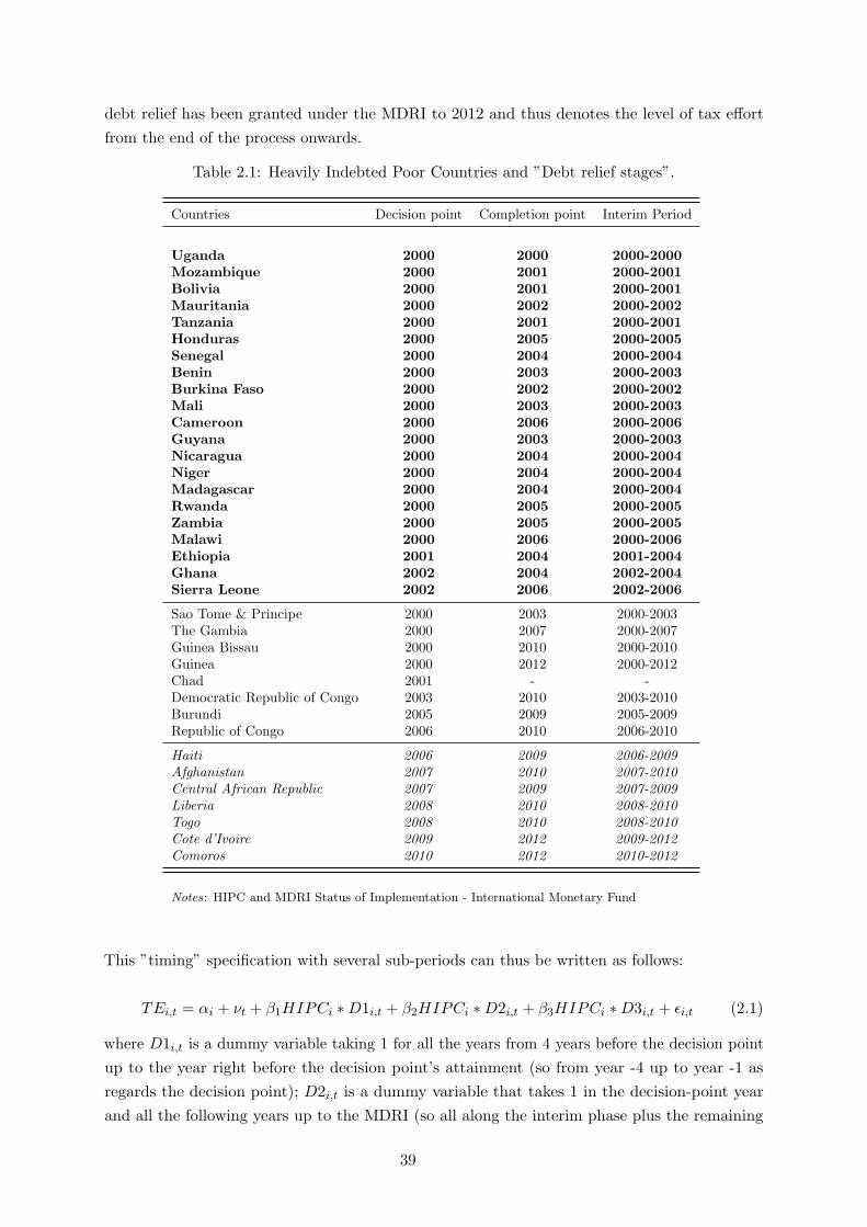
debt relief has been granted under the MDRI to 2012 and thus denotes the level of tax effort

from the end of the process onwards.

Table 2.1: Heavily Indebted Poor Countries and ”Debt relief stages”.

Countries Decision point Completion point Interim Period

Uganda 2000 2000 2000-2000Mozambique 2000 2001 2000-2001Bolivia 2000 2001 2000-2001Mauritania 2000 2002 2000-2002Tanzania 2000 2001 2000-2001Honduras 2000 2005 2000-2005Senegal 2000 2004 2000-2004Benin 2000 2003 2000-2003Burkina Faso 2000 2002 2000-2002Mali 2000 2003 2000-2003Cameroon 2000 2006 2000-2006Guyana 2000 2003 2000-2003Nicaragua 2000 2004 2000-2004Niger 2000 2004 2000-2004Madagascar 2000 2004 2000-2004Rwanda 2000 2005 2000-2005Zambia 2000 2005 2000-2005Malawi 2000 2006 2000-2006Ethiopia 2001 2004 2001-2004Ghana 2002 2004 2002-2004Sierra Leone 2002 2006 2002-2006

Sao Tome & Principe 2000 2003 2000-2003The Gambia 2000 2007 2000-2007Guinea Bissau 2000 2010 2000-2010Guinea 2000 2012 2000-2012Chad 2001 - -Democratic Republic of Congo 2003 2010 2003-2010Burundi 2005 2009 2005-2009Republic of Congo 2006 2010 2006-2010

Haiti 2006 2009 2006-2009Afghanistan 2007 2010 2007-2010Central African Republic 2007 2009 2007-2009Liberia 2008 2010 2008-2010Togo 2008 2010 2008-2010Cote d’Ivoire 2009 2012 2009-2012Comoros 2010 2012 2010-2012

Notes: HIPC and MDRI Status of Implementation - International Monetary Fund

This ”timing” specification with several sub-periods can thus be written as follows:

TEi,t = αi + νt + β1HIPCi ∗D1i,t + β2HIPCi ∗D2i,t + β3HIPCi ∗D3i,t + ǫi,t (2.1)

where D1i,t is a dummy variable taking 1 for all the years from 4 years before the decision point

up to the year right before the decision point’s attainment (so from year -4 up to year -1 as

regards the decision point); D2i,t is a dummy variable that takes 1 in the decision-point year

and all the following years up to the MDRI (so all along the interim phase plus the remaining

39

carefully identified.

Selection issue

First, given that debt relief is not randomly assigned, selection into the treatment can

potentially weaken the identification strategy. As explained above, the IFIs defined eligibility

criteria to flag countries supposed to be the “best candidates” for these debt cancellations. A

relevant control group should thus be made up of countries that satisfied these eligibility criteria,

but were ultimately not granted debt relief under the HIPC initiatives. Consequently, I first

define a “narrow control group” including countries that might have been eligible or close to

eligible for the debt relief process, but which ultimately did not benefit from the HIPC initiatives.

The selection criteria are: 1) having an average debt-to-exports ratio of over 170% (in face

value)6 over the four years before 1996 (the HIPC’s announcement year), and 2) having been

ranked as a low income country by the World Bank for at least three years between 1992 and

1996. Table 2.B1 (p.68) in the Appendix B displays the countries that satisfy these selection

criteria and hence form the narrow control group. We observe that almost all the countries were

ranked LICs before 1996, and thus benefited from an IMF economic program where a strong

emphasis was also put on domestic revenue mobilization. However, one can notice that the

average debt-to-exports ratio before 1996 was significantly lower than it is for the HIPCs. This

might explain in why these countries never benefited from the multilateral debt relief initiatives

and remained “untreated”.

In addition, I also define two additional control groups: the “extended control group” and

the “African control group”. The first one includes all non-HIPC developing countries (ranked

at least once as LICs over the four years before 1996) and hence controls for a potential trend

in tax effort within the “developing world”. Yet given that out of 39 HIPCs, 33 are African

countries (22 out of 26 in our sample), I also consider an “African control group”. This group

contains all non-HIPC African developing countries, and thus controls for a potential trend in

tax performance within the continent. Sample composition of the extended and African control

groups is provided in Table 2.B2 (p.69) in the Appendix B.

Yet, most of the countries that satisfied the eligibility criteria benefited from the Enhanced

HIPC initiative. Every eligible country indeed received a proposal from the IFIs to join the debt

relief process. Some countries such as Laos refused to participate in the initiative because of the

debt forgiveness conditionality terms set by the IMF and the World Bank.7 So there is no perfect

counter-factual such as a country that would have been eligible for the initiative, was willing to

participate, and ultimately did not benefit from it. In this case, endogeneity issues would result

from the fact that treated countries have both observable and unobservable characteristics that

drove them being granted debt relief under the Enhanced HIPC initiative. In order to reduce

this risk of selection bias, I suggest alternative methods such as considering as control countries

the HIPCs that entered late the initiative. This leads to adopt a “pipeline approach” where

6It would have been better to use the threshold in NPV, but long time series on such data are not availableand computing them would have exposed this criterion to questionable assumptions regarding the discount rate.The rate of 170% for the debt-to-exports ratio thus intentionally overshoots the required threshold of 150% inNPV to partly account for the grant element in the nominal debt.

7So did Ghana initially, before agreeing to debt relief in 2002. However, the Ghana’s refusal was mostlymotivated by fears associated with an increase in interest rates after debt relief.

41

control units are the ones which have not been treated in the first place, but which will benefit

from the treatment later on. Lastly, I also resort to propensity score methods to identify control

group countries with similar (on average) ex-ante likelihood of being granted debt relief.

Omitted variables bias

The second channel through which endogeneity could mar the identification strategy is the

omitted variable bias. It is indeed likely that a third factor (observable or not) simultaneously

explains participation (or non-participation) in the debt relief program and the variation in

governments’ tax effort. To reduce the omitted variable bias as much as possible, I control for

numerous variables in the zero-stage estimate where tax effort index are obtained. This zero-stage

estimate provides a measure of the government’s willingness to tax, which is filtered using various

macroeconomic indicators such as GDP per capita, openness rate, sectoral composition of the

economy, rate of inflation and so on, which could be correlated with both treatment and the

government’s tax effort. Tax effort estimates also include country and time fixed effects that

capture the contributions of unobserved (time-invariant) country-specific features and changes

due to time trends or common shocks.

In addition, althought the classic DID specification usually includes a dummy variable for

HIPCs only —in order to account for the initial discrepancy in tax effort between the “treated”

and the “untreated”—, I favor DID estimates with country-fixed effects to better address any

country-specific (time-invariant) unobservables that might influence the relationship between

debt relief provision and tax effort. These estimates thus provide the average within-country

variation in tax effort for HIPCs, around different debt relief stages, and as compared with the

average tax effort evolution in control-group countries.8

Reverse causality

Lastly, a major endogeneity concern usually takes the form of potential simultaneity whereby

the outcome variable also affects the treatment, making the identification of a causal effect

impossible if it is not controlled for. I acknowledge that given the design of the HIPC process,

and the required eligibility criteria, tax effort performances potentially affect the attainment of

the decision point. Such conditionality effect should thus be captured by β1 in equation 2.1. If

true, then a positive coefficient associated with β2 should be carefully interpreted since such

increase could be attributed either to a debt overhang effect or to a legacy stemming from the

tax improvements made ex-ante. However, I assume tax effort changes following debt relief under

MDRI (so β3) are less exposed to reverse causality since the 2005 decision of canceling the whole

remaining multilateral debt stock was mainly politically driven in view of reaching the MDGs by

2015. Therefore, although some observables (and unobservables) might still explain why some

HIPCs have completed their interim period earlier, and thus benefited from debt relief under the

MDRI earlier than other HIPCs (which has more to do with the selection issue exposed above),

we think simultaneity between tax effort performance and ultimate debt forgiveness under the

MDRI is less plausible than in the case of the decision point attainment.

I thus start by simply looking at the tax effort evolution around the different stages of the

8I also ran all estimates with an HIPC dummy variable in order to observe the differential effects on tax effortof the different stages of the HIPC process between HIPC and non-HIPC countries. Estimates support our resultswithout the HIPC dummy and are available upon request to the author.

42

debt relief process using equation 2.1, and then, as explained above, consider alternative control

groups and specifications to control as much as possible for selection into the debt relief initiative

and to investigate the effect of the overall debt relief initiatives (and of the MDRI in particular)

on tax effort.

2.3.2 What is tax effort and how can we measure it?

How can we define the government’s willingness to tax? Many studies have attempted to

measure it using proxies and zero-stage estimate procedures. In keeping with the definition

provided by Gupta (2007), I consider for this study the classic tax effort measure computed

as the ratio of actual to potential tax revenues. This measure of tax effort can be considered

as the effort made by a government to collect what its economy potentially supplies. The

extent of a country’s tax base depends on its economic, social, demographic and even historical

characteristics which therefore determine potential tax revenues, or, in other words, the country’s

“tax capacity” (Fenochietto and Pessino, 2013). So if a gap is found between what the government

can levy (taxes predicted by economic and social outcomes) and what it actually collects (actual

tax revenues), this shortfall in domestic revenues could be said to be due to the government’s

inadequate tax collection efforts and could therefore be associated with a weak will to raise

domestic resources. Consequently, any tax effort ratio (actual taxes over predicted taxes) inferior

to one means that the government falls short of its “tax capacity” and can be interpreted as a

weak willingness to tax.

Although this tax effort ratio might be subject to measurement errors (Baskaran and Bigsten,

2013), it represents an interesting proxy for the government’s willingness to tax since it denotes

the deviation from current tax level, which is exogenous to structural tax determinants. I

therefore keep it as the preferred measure and build tax effort index using predicted taxes

stemming from an estimation (zero-stage estimate) where the tax-to-GDP ratio is explained

by per capita GDP, the openness rate, the share of agriculture and natural resources in the

economy, and some demographic factors such as the population density, the age dependency

ratio and the urbanization rate. Data used for the calculation of tax effort come from both IMF

documents and the World Development Indicators (WDI) database (see Appendix A, p.64, for

details on the methodology).

However, other proxies might also be considered. In their paper on the impact of government

fiscal capacity on institutional quality in Sub-Saharan Africa, Baskaran and Bigsten (2013) use

several measures for government fiscal capacity besides this classic tax effort measure. They first

argue that fiscal capacity can be proxied by total tax revenues given that domestic resources in

these countries rely to a large extent on non-tax revenues such as natural resources revenues

(Burgess and Stern, 1993). Yet, total taxes do not appear to be the more suitable proxy since

economic fluctuations such as unexpected increase in imports with no changes in GDP would

increase the amount of tax collected (through taxes on international trade) and therefore the

tax-to-GDP ratio without reflecting a genuine change in the government’s willingness to tax.

Considering the low rate of tax compliance in developing countries (Fjeldstad and Therkildsen,

2008), Baskaran and Bigsten (2013) then suggest taking income taxes, as it could be interpreted

as a real government effort if it were to increase. But the state of disaggregated tax data

43

availability in developing countries makes it hard to collect long, full time series on direct and

indirect taxes for our entire sample (HIPCs and control group countries), which prevents from

using it as the benchmark proxy for the government’s tax effort. Nevertheless, this paper looks at

a newly released dataset on disaggregated taxes and reviews this alternative measure in section

4. It finds similar results to those obtained with the estimated tax effort measure.

2.3.3 Visual examination

Figures 2.3 and 2.4 below represent the change in tax revenues (% of GDP) and tax effort

around the decision point and can provide preliminary insight into the impacts of debt relief.9

The solid black line in Figure 2.3 denotes the average tax-to-GDP ratio for HIPCs that reached

their decision point no later than 2003.10 The difference in tax share between the baseline

period, the anticipatory phase and the post-decision point period seems to be clearly positive

for HIPCs, which confirms the findings of Cassimon et al. (2015). However, looking at changes

in average tax share for control groups, one can see that this increase could be due to a trend

among LICs since a increasing evolution in tax-to-GDP ratio is also observed for the different

control groups over the years following the decision point. Taking a closer look at these graphs,

an acceleration in the tax-to-GDP ratio for HIPC countries can nonetheless be found in the

years of the anticipatory phase (which for most of the sample, coincide with the years following

the HIPC announcement date). Yet, this is not really observed for other control groups and

might reflect an increase in tax effort motivated by the conditionality attached to the initiative

(which calls for tax raising improvements to be made to enter the debt relief program and secure

future debt cancellations). This ex-ante evolution seems to be also supported by Figures 2.4

where tax-to-GDP ratios are replaced by tax effort index.

2.3.4 Control groups suitability

Looking quickly at the macro-covariates for control groups before 1996, the HIPCs appear

to remain quite different in terms of GDP per capita, breakdown of economic activity, and

demographic features (cf. Table 2.B3 in the Appendix B, p.70). However, the data suggest that

the narrow control group displays economic features closest to the HIPCs, which comforts the

decision of considering this control group as the preferred counterfactual. Focusing then on

Figures 2.4 below and 2.B1 in the Appendix B (p.71), HIPCs and control group countries seem

to experience similar tax effort trends throughout the anticipatory phase. The parallel trend

hypothesis over the years preceding the “treatment effects” (which can be both ex-ante and

ex-post in our context) is necessary for the reliability of DID estimates.

Consequently, in addition to this visual examination, I run placebo tests to check for ex-ante

parallel trends between control and treatment groups. I thus estimate a model where the change

in tax effort between years -8 and -5 as regards the decision point is compared with the period

prior year -9, and with respect to tax effort evolution in the different control groups. I also

define an alternative placebo test, where the baseline period is split up in half for HIPCs, as if a

placebo treatment was granted halfway this period, and for HIPCs only. The specifications used

9The methodology used to build those graphs is detailed in the Appendix E, p.86.10Note that considering all HIPCs in the sample (regardless their decision point’s date) leads to similar graphs.

44

respect to the three different control groups and for two HIPCs samples. The HIPCs sample 1

is the one considering 26 HIPCs having reached their decision point not later than 2003. This

restriction is motivated by the need for a long-enough post-decision point period, necessary to

observe how tax effort varies throughout the extended interim period and after the MDRI. Yet

this restriction implicitly results in selection into “the highest performance HIPCs” treatment

group which managed to rapidly implement a PRGF to secure debt relief in the early 2000s.12 I

thus also present results when considering all HIPCs in the sample, regardless of their date of

entry into the HIPC process (i.e. 34 HIPCs13).

Table 2.2: Main results.

(I) (II) (III) (IV) (V) (VI)

Dep. var.: Tax effort index

HIPC sample 1 HIPC sample 2

Control group: Narrow Extended African Narrow Extended African

HIPC*D1: (Anticipatory effect) 0.194*** 0.145*** 0.137*** 0.143*** 0.108*** 0.099***(4.085) (4.837) (4.669) (4.935) (3.935) (3.571)

HIPC*D2: (DP-MDRI period) 0.353*** 0.220*** 0.239*** 0.267*** 0.187*** 0.190***(7.536) (7.516) (5.887) (7.409) (7.554) (6.027)

HIPC*D3: (post-MDRI period) 0.183*** 0.109*** 0.092** 0.161*** 0.097*** 0.085**(4.152) (5.132) (2.298) (4.201) (3.653) (2.431)

Constant 0.811*** 0.943*** 0.885*** 0.623*** 0.657*** 0.612***(14.721) (18.905) (12.002) (8.272) (5.957) (6.098)

Observations 854 2,135 916 1,008 2,289 1,070No. of HIPCs 26 26 26 34 34 34

No. of control countries 14 78 17 14 78 17Country fixed effects Yes Yes Yes Yes Yes Yes

Time fixed effects Yes Yes Yes Yes Yes YesR-squared 0.166 0.086 0.129 0.138 0.083 0.114

Test: D2 - D1 = 0 (p-val.) 0.000 0.003 0.007 0.000 0.000 0.002Test: D1 - D3 = 0 (p-val.) 0.790 0.143 0.208 0.320 0.588 0.702Test: D2 - D3 = 0 (p-val.) 0.000 0.000 0.002 0.031 0.000 0.001

Notes: Estimates have been obtained using the option vce(bootstrap) under STATA 13. F-statistics are not reported here but areall significant at the 5% level. Columns (I), (II), and (III) report estimate results of equation 2.1 where the sample consideredincludes 26 HIPCs having reached their decision point no later than 2003. Columns (IV), (V), and (VI) expose estimate resultsof equation 2.1 when the HIPCs sample is not restricted and includes all HIPCs, regardless their decision point’s date. Taxeffort index measured at the country-year level are obtained from structural tax equation 2.2 (column (1) in Table 2.A2). Taxeffort estimates using specification of column (1) in Table 2.A2 are quite large for Niger, leading thus to inflated results. Wetherefore removed Niger from our main estimates and provide estimate results including Niger figures in the Appendix E (Cf.Table 2.E1, p.86). We next do not provide results with Niger since they follow those reported throughout the study (but are justlarger in magnitude). However, remaining Tables with Niger are available upon request to the author. The last three rowsexpose tests for difference in coefficients. The first one reports the significance (p-value) of the difference between D2 andD1 coefficients. The second row compares D1 and D3 coefficients, while the last one exposes the significance of the differencebetween D2 and D3 coefficients. Robust z-statistics are exposed in parentheses. ***, ** and * denote significance at 10%, 5%and 1%.

12However, one could also think that political motives lie behind the early provision of debt relief under theEnhanced HIPC initiative.

1334 HIPCs having at least reached their decision point. Haıti is excluded because of the 2010 earthquakewhich clearly changes the country’s economic structure and makes it impossible to observe a clear-cut relationshipbetween tax effort and debt relief.

47

Results suggest that HIPCs start improving their tax effort before the decision point (through-

out the anticipatory phase), sustain this effort during their extended interim period (from the

decision point to the MDRI) and even after receiving ultimate debt relief under the MDRI.

Within HIPCs, tax effort increases by between 9 to 18 additional percentage points after the

MDRI as compared with the level recorded over the baseline period. This pattern is robust

when comparing tax effort changes within HIPCs, with the ones in narrow, extended or African

control groups’ countries. In addition, the right part of the Table shows that results obtained

for the benchmark HIPCs sample (column (I) to (III)) are similar to those when all HIPCs are

considered (columns (IV) to (VI)).14

However, one can notice that the level of tax effort in the extended interim period is greater

than the one recorded for the anticipatory phase. Indeed, looking at the tests performed at

the bottom of Table 2.2, we observe that coefficients associated with D2 are significantly larger

(in all regressions) than those for the anticipatory phase. This could mean that while HIPCs

deploy significant tax effort to become eligible for the Enhanced HIPC initiative, the provision

of debt relief fosters them in reaching higher levels of tax effort throughout the extended interim

period. Yet one could conversely argue that the larger tax effort observed over this period simply

results from tax reforms undertaken under the anticipatory phase which come to finally benefit

to HIPCs’ governments few years after (thus during the extended interim period).

Interestingly, the other tests on coefficients suggest that HIPCs, on average, ease off their

tax policies once they received full and irrevocable debt relief. Indeed, coefficients associated

with the post-MDRI period (D3) are significantly lower than those for the extended interim

period (D2). Such an effect could be expected in HIPCs, since the completion point marks

the end of the Enhanced HIPC process and therefore the end of the conditionality linked to

debt relief provision. Now that the government has secured debt forgiveness and is not under

IMF and World Bank ”supervision” anymore, it can basically decide to go back to old policies,

slacken off on domestic resource mobilization and look for new domestic or foreign financing

opportunities, reinforcing moral hazard. Such behavior might have also been made possible by

the attitude of the IMF regarding fiscal policies in Sub-Saharan African countries which seems

to have somewhat relaxed at then end of the 2000s according to some economists.15 At first

glance, these results thus seems to support evidence of zigzag behaviors by HIPCs, as suggested

by Easterly (2002).

Nevertheless, although the drop in tax effort observed after the MDRI produces an average

tax effort inferior to the one recorded in the extended interim period, the second row from

the bottom of Table 2.2 shows that there is no significant difference in tax effort between

the anticipatory phase and the post-MDRI period. Indeed, it seems that the combination of

anticipatory effects with larger tax effort in the extended interim period offsets the negative

impact of having been granted debt relief under the MDRI. Strictly speaking, this means that,

within HIPCs, the tax effort in the post-MDRI years is significantly larger than the level recorded

in the years preceding the anticipatory phase (so over the baseline period).

14Note that removing the seven countries which benefited from the original HIPC initiative from the HIPCssample 1 and 2, does not change the results. Results are not reported in order to save space but are availableupon request.

15See the Rodrik’s letter addressed to Andrew Berg on this topic: http://rodrik.typepad.com/dani_rodriks_weblog/2009/05/the-kinder-gentler-imf-on-african-fiscal-policy.html

48

The findings therefore suggest that greater tax efforts after the completion point are a de facto

legacy of efforts in the years preceding the decision point and during the extended interim period.

Under these circumstances, conditionality makes beneficiary country significantly improve their

fiscal outcomes. The results hence argue in favor of conditionality when granting debt relief

to LICs, which contradicts the findings of existing literature on the effectiveness of the IMF’s

programs (Przeworski and Vreeland, 2000; Bird and Rowlands, 2001; Easterly, 2005; Dreher,

2006).16 Moreover, conditionality is more likely to succeed under the HIPC initiatives’ settings

since the outcome for compliant countries is more attractive than in classic IMF programs.

Indeed, while conditionality under IMF programs leads to new concessional loans, i.e. new debts,

conditionality under debt relief programs gives rise to debt cancellations. Therefore, HIPCs

would be more disposed to efficiently conduct reforms when they expect future debt relief, which

in fine produces significant results on the targeted outcomes.

2.4.2 Validity of control groups and selection issues

Alternative control groups

Up to this point, the comparison with the extended and African control groups shows

that tax effort changes around the debt relief process are not driven by an increasing trend in

developing or African countries. However, there could be some doubts about the level of the

cutoffs considered to identify narrow control group countries. I thus test the robustness of the

first results to these selection criteria, using different cutoffs in terms of debt ratio and income

classification.

As presented in Section 2, the IFIs also defined indebtedness threshold in fiscal terms for

really open countries that did not satisfy the 150% debt-to-exports ratio, even though their

external public debt was burdensome.17 The required debt ratio for this particular type of

country was set to 250% of their domestic revenues (in NPV). Consequently, I first define a new

control group called “PANEL A” comprising countries with an average debt-to-revenue ratio

superior to 250% over the six years preceding 1996, and which the World Bank classified as LIC

for at least four years out of these six. I then define as “PANEL B”, countries classified as IDA

eligible-only for at least four years between 1990 and 1996, regardless their indebtedness level.

Using the indebtedness historical classification provided by the World Bank, I also determine

two control groups (“PANEL C” and “PANEL D”) where countries classified for at least four

years between 1990 and 1996 as Moderately or Severely Indebted (excluding HIPCs of course) are

included in “PANEL C”. “PANEL D” only considers those defined as Severely Indebted. The

composition of these four control groups, as well as the definition of Severely and Moderately

Indebted countries, is provided at the beginning of the Appendix C (p.74).

However, although these countries posted similar economic characteristics in the years

preceding 1996 (in terms of income classification and indebtedness ratio), comparisons with

these additional control groups do not completely clear all doubts about the similarities between

HIPCs and control group countries. Indeed, the simple fact that they did not benefit from

16Note, however, that these papers focus mainly on the effects of IMF conditionality on economic growth andnot fiscal outcomes.

17Countries like Senegal or Cameroon for instance (Bougouin and Raffinot, 2003).

49

the initiative makes them different from the HIPCs. Therefore, another attempt to control for

potential selection bias would be to define a control group made up solely of “future HIPCs”,

i.e. countries that entered the Enhanced HIPC process late and that, although eligible for the

initiative in the early 2000s, only benefited from it later on.18 Using this control group would

call for a sort of “pipeline approach” commonly used in experimental economics whereby the

control group is made up of individuals eligible for the treatment, but not randomly chosen to

benefit from the treatment in the first stage, and who will benefit from it later on (althought the

random feature is largely debatable in the present case). Consequently, “Panel E” comprises all

the HIPCs, and results for this sample simply consist in estimates of equation 2.1 where we only

consider HIPCs in the study sample (since HIPCs reached their decision point and benefit from

the MDRI at different dates).19 However, the small number of “untreated” units in this control

group is reducing over time (since more and more HIPCs reach their decision point and then

benefit from the MDRI as we get close to the end of the period) which means that the result

need to be viewed with caution, even though they can provide further insights into the effect of

the debt relief initiatives on recipient countries’ tax effort.

Table 2.3 presents results with the different control groups. Results significantly support the

previous findings for our main control groups. However, we note that coefficients associated with

the post-MDRI period become not significant when comparing HIPCs with heavily indebted

non-HIPCs, and when we adopt the ”pipeline approach”, which supports the evidence of a

stronger moral hazard and average zigzag behavior once countries leave the HIPC process and

are granted massive and irrevocable debt relief under the MDRI.

PSM-based control groups

Although these multiple comparisons with different control groups may suggest that debt

relief granted under the HIPC initiatives has indeed affected tax effort in recipient countries,

question marks could still hang over the effect of this debt relief program since, as described in

Section 2.3.4, the narrow control group, although the closest from HIPCs (in average) in terms

of economic characteristics, remains significantly different from the “treatment” group as regards

the observables considered and observed before 1996.

A final attempt to reduce the bias stemming from the selection into the debt relief initiative,

consists in identifying a control group of countries with high probability of receiving debt relief

under the HIPC initiatives. I thus estimate a Probit model where the probability of being an

HIPC (and so having been granted debt relief under these initiatives) is explained by ex-ante

covariates, averaged before 1996. That way, the propensity score of being “treated” is only

determined by economic (and political) characteristics observed before the debt relief initiative’s

announcement and allows to find control units with similar macroeconomic features during the

pre-1996 period. I consider economic characteristics (averaged over 1990-1996) which could

explain both the probability of receiving debt relief and the initial tax effort performance.

Regarding the determinants of being an HIPCs, I first choose the debt level as well as the level

18Although the random feature of such stepwise treatment cannot be applied in the present case.19Cf. Table 2.1 (p.39). Haiti is excluded for the reasons previously exposed. However, while we include Eritrea

and Sudan that are defined as HIPCs in pre-decision point phase, we do not include Somalia which has the samestatus, because of lack of data.

50

Table 2.3: Alternative control groups.

(I) (III) (IV) (V) (VI)

Dep. var.: Tax effort index

HIPCs sample 1

Control group: Panel A Panel B Panel C Panel D Panel E

HIPC*D1: (Anticipatory effect) 0.206*** 0.185*** 0.135*** 0.103*** -(5.556) (5.701) (3.523) (2.632) -

HIPC*D2: (DP-MDRI period) 0.402*** 0.257*** 0.252*** 0.228*** -(8.652) (7.794) (6.178) (5.464) -

HIPC*D3: (post-MDRI period) 0.202*** 0.131*** 0.148*** 0.068 -(4.084) (3.979) (4.113) (1.451) -

Constant 0.817*** 0.959*** 0.931*** 0.850*** -(14.878) (13.972) (15.827) (16.960) -

Observations 764 1,333 969 750 -No. of HIPCs 26 26 26 26 -

No. of control countries 10 37 21 11 -Test: D2 - D1 = 0 (p-val.) 0.000 0.023 0.003 0.003 -Test: D1 - D3 = 0 (p-val.) 0.913 0.119 0.714 0.448 -Test: D2 - D3 = 0 (p-val.) 0.000 0.000 0.006 0.000 -

HIPCs sample 2

Control group: Panel A Panel B Panel C Panel D Panel E

HIPC*D1: (Anticipatory effect) 0.151*** 0.133*** 0.109*** 0.084*** 0.080**(5.339) (4.770) (4.182) (2.799) (2.224)

HIPC*D2: (DP-MDRI period) 0.287*** 0.211*** 0.214*** 0.182*** 0.164***(10.111) (7.466) (6.496) (5.190) (3.517)

HIPC*D3: (post-MDRI period) 0.173*** 0.115*** 0.140*** 0.079* 0.003(3.991) (3.560) (3.804) (1.743) (0.043)

Constant 0.635*** 0.656*** 0.657*** 0.645*** 0.620***(7.613) (7.456) (7.586) (7.099) (7.402)

Observations 918 1,487 1,123 904 739No. of HIPCs 34 34 34 34 37

No. of control countries 10 37 21 11 -Test: D2 - D1 = 0 (p-val.) 0.000 0.010 0.001 0.000 0.003Test: D1 - D3 = 0 (p-val.) 0.543 0.515 0.341 0.906 0.092Test: D2 - D3 = 0 (p-val.) 0.001 0.000 0.016 0.005 0.000

Notes: Estimates have been obtained using the option vce(bootstrap) under STATA 13. F-statistics are notreported here but are all significant at the 5% level. We also expose results for the two HIPCs’ samples.HIPCs sample 1 only considers HIPCs having reached their decision point no later than 2003. HIPCs sample2 includes all HIPCs regardless their decision point’s date. Panel A (average debt-to-revenue ratio ≥

250%, and LIC classification at least 4 years between 1990-1996), Panel B (IDA-eligible onlybefore 1996), Panel C (Moderately or Severely Indebted before 1996), Panel D (SeverelyIndebted before 1996), Panel E (All HIPCs). Tax effort index come from structural tax equation2.2 (column (1) in Table 2.A2, p.67). Robust z-statistics are exposed in parentheses. ***, ** and * denotesignificance at 10%, 5% and 1%.

51

of GNI per capita. Indicators of the country’s economic structure such as the share of the

agricultural sector, the exports, imports, or natural resources into the GDP are also included into

the model. I then add the density of the population (in log) as well as aid grants (net from debt

relief grants and expressed in percentage of GDP). Lastly, I augment the Probit model with the

level of tax effort before 1996 and a measure of institutional quality (Polity IV index) since it has

been shown as determining the access to these initiatives (Freytag and Pehnelt, 2009; Presbitero,

2009). I then derive propensity scores from Probit estimates, and restrain the control group to

non-HIPCs with a propensity score superior or equal to 0.2 (with the control group’s composition

varying according to the specification considered). More details about the model specification is

provided in the Appendix C (p.74). Table 2.C2 in the Appendix C (p.77) shows that considering

non-HIPCs with a propensity score above 0.2 leads to a control group with average ex-ante

economic characteristics quite similar to those of HIPCs. However, the average ex-ante level of

tax effort and propensity score for HIPCs remain both significantly different from those of control

group countries (on average) across the different Probit specifications. Consequently, I define

another control group where are only included non-HIPCs with a propensity score superior to

0.5 and for which economic features are even closer from those of HIPCs. Nevertheless, reducing

the control group sample to countries with higher propensity score leads to consider much less

control countries (7 - 10) which is why Table 2.4 reports results as compared with the two

propensity score-based control groups.

Looking at Table 2.4 above, results of the DID equation with propensity score-based control

groups20 support previous findings, i.e. an increase in tax effort during the anticipatory and

extended interim periods (which here, are similar in magnitude). Moreover, results also confirm

findings stemming from the previous robustness check; i.e. HIPCs loosen their tax effort once

they have benefited from debt relief under the MDRI, which here, leads them to a tax effort

level which is not statistically significant from the one recorded over the baseline period.

20Where propensity scores have been obtained from different specification in order to test the robustness of theeffects to the composition of the PSM-based control group.

52

Table 2.4: Propensity score- based control groups.

(I) (II) (III) (IV) (V) (VI)

Dep. var.: Tax effort index

CG selection based on: Propensity score ≥ 0.2 Propensity score ≥ 0.5

Probit model: (1) (2) (3) (1) (2) (3)

HIPC*D1: (Anticipatory effect) 0.144*** 0.155*** 0.174*** 0.106** 0.117** 0.130***(3.337) (4.551) (4.862) (2.323) (2.402) (2.899)

HIPC*D2: (DP-MDRI period) 0.202*** 0.204*** 0.263*** 0.128** 0.164*** 0.215***(4.591) (6.580) (6.982) (2.371) (2.999) (4.253)

HIPC*D3: (post-MDRI period) 0.037 -0.002 0.077** -0.116** -0.075 -0.014(0.884) (-0.046) (2.354) (-2.257) (-1.430) (-0.303)

Constant 0.819*** 0.843*** 0.834*** 0.813*** 0.821*** 0.838***(15.318) (11.535) (18.551) (12.198) (14.940) (15.196)

Observations 1,043 900 802 726 764 690No. of HIPCs 26 26 26 26 26 26

No. of control countries 23 16 12 8 10 8Test: D2 - D1 = 0 (p-val.) 0.127 0.108 0.013 0.647 0.202 0.039Test: D1 - D3 = 0 (p-val.) 0.005 0.000 0.014 0.000 0.000 0.001Test: D2 - D3 = 0 (p-val.) 0.000 0.000 0.000 0.000 0.000 0.000

Notes: Estimates have been obtained using the option vce(bootstrap) under STATA 13. F-statistics are not reportedhere but are all significant at the 5% level. We expose results for the HIPCs sample 1 where we only considersHIPCs having reached their decision point no later than 2003. Results with HIPCs sample 2 are similar andavailable upon request to the author. Columns (I) to (III) shows DID coefficients when the control groups includesnon-HIPCs with a propensity score superior to 0.2. Columns (IV) to (V) reports DID coefficients when consideringnon-HIPCs with a propensity score above 0.5 as control units. The different Probit models refers to the various setof control variables alternately used to estimate propensity scores (cf. Appendix C, p.74). Tax effort index comefrom structural tax equation 2.2 (column (1) in Table 2.A2, p.67). Robust z-statistics are exposed in parentheses.***, ** and * denote significance at 10%, 5% and 1%.

2.4.3 Validity of the tax effort’s measure

Testing for different tax effort estimates

I then test the results using alternative dependent variable. As explained in Section 2.4, the

preferred tax effort measure is drawn from column (1) specification in Table 2.A2 (p.67) and the

PCSE estimators, which both take into account heteroskedasticity and serial autocorrelation

issues (cf. Appendix A, p.64). Given that being granted debt relief has a positive ex-ante and

ex-post impacts on HIPC governments’ tax efforts when it is determined by this estimate of

tax effort, it would be interesting to know whether these effects hold when replacing tax effort

index based on the PCSE estimators by tax effort index obtained using alternative zero-stage

specification and estimators.

Equation 2.1 is then re-estimated, but now with different measures of tax effort derived

from the structural tax specification (3) (using alternately PCSE and LSDV estimators) in

53

Table 2.A2. As with the benchmark specification, average tax effort appears to increase over the

anticipatory phase, improve even further during the extended interim period, and then lowers

after the MDRI.21 Results remain robust to the different control groups considered all along this

study and also hold when switching for the propensity score-based control groups.22

Non-estimated tax effort proxies

So far, I have used a zero-stage estimated tax effort variable to represent the government’s

willingness to tax. However, as already explained, this variable is subject to measurement

errors that may still fuel doubts over these findings. I therefore use disaggregated tax variables

retrieved from the Government Revenue Dataset (GRD, ICTD) (Prichard et al., 2014), which

contains disaggregated tax data for a large number of developing countries. This dataset basically

builds on the same sources as the one used for the benchmark tax effort measure, but has the

disadvantage of still having a sizable number of missing values.23 Regarding disaggregated tax

data, over a fifth of the information is missing, especially for HIPCs. This rules out the use

of this dataset for main estimates. Nevertheless, consideration of the impact of the debt relief

process on disaggregated tax variables can make for interesting additional robustness checks.

I focus on two types of disaggregated taxes that may reflect the government’s willingness to

tax: indirect and direct taxes (both excluding natural resource revenues). Among the indirect

taxes, taxes on goods and services can be considered as a good proxy for government willingness

to tax since increases in VAT and sales tax are partly associated with economic performance,

but also largely depend on the quality and efficiency of the tax administration in supervising

self-assessed tax returns. With respect to direct taxes, the aggregated variable appears to also

be a good proxy for the government’s willingness to tax since collecting taxes on incomes and

profits in developing countries necessitates close tax administration oversight.

I therefore run DID models taking these disaggregated taxes as dependent variables. Yet in

keeping with Mahdavi (2008), disaggregated taxes such as direct and indirect taxes have been

shown to be affected by the economic environment. I therefore run equation 2.1, adding the

same control variables as in the structural tax specification (specification of column (1) in Table

2.A2).

Table 2.5 shows the results for indirect taxes; and for its component on goods and services

since there is no effect on direct taxes nor on international trade-related taxes. Results suggest

that foreseeing debt relief and having been granted it over the extended interim period leads to

an increase in indirect taxes by around 1 to 2 additional GDP percentage points. The effect

of debt relief on indirect taxes also seems to go through taxes on goods and services (since no

effect is observed for international trade-related taxes) which is in line with the advices of the

Decision-Point documents. This means that the positive effect on indirect taxes could also stem

from the conditionality attached to the HIPC initiative.

21Table 2.C5 in the Appendix C (p.79) reports the results. Note that DID results with tax effort index obtainedfrom other specifications ((2), and (4)) and with both estimators (LSDV and PSCE) are not reported to savespace, but are similar to those reported in Table 2.C5, and are available upon request.

22Results are not reported in order to save space but are available upon request to the author.23See Table 2.C4 in the Appendix C, p.78. Note that the pairwise correlation between the variable of tax

revenues excluding natural resources revenues (obtained from IMF Staff Report) and the one from the ICTDdataset is equal to 76.3% supporting hence the reliability of our own dataset.

54

Table 2.5: Alternative tax effort measures - Using disaggregated taxes.

(I) (II) (III) (IV) (V) (VI)

Dep. var.: Indirect tax-to-GDP ratio

HIPC sample 1 HIPC sample 2

Control group: Narrow Extended African Narrow Extended African

HIPC*D1: (Anticipatory effect) 1.247*** 1.106*** 1.409*** 0.620** 0.689** 0.736**(2.976) (3.106) (3.533) (2.172) (2.151) (2.218)

HIPC*D2: (DP-MDRI period) 1.883*** 1.771*** 2.064*** 1.320** 1.433*** 1.359**(3.166) (3.282) (3.163) (2.502) (2.911) (2.270)

HIPC*D3: (post-MDRI period) 1.170 1.887** 1.396 0.844 1.530** 0.861(1.399) (2.574) (1.379) (1.078) (2.325) (0.939)

Constant 21.571 21.331*** 9.641 0.694 17.521** -6.148(0.886) (3.044) (0.750) (0.049) (2.177) (-0.501)

Observations 700 1,822 775 834 1,956 909No. of HIPCs 26 26 26 34 34 34

No. of control countries 12 75 16 12 75 16R-squared 0.870 0.883 0.885 0.906 0.880 0.879

Dep. variable: G&S tax-to-GDP ratio

HIPC sample 1 HIPC sample 2

Control group: Narrow Extended African Narrow Extended African

HIPC*D1: (Anticipatory effect) 0.726** 0.372 0.844** 0.345 0.080 0.364(2.473) (1.126) (2.324) (1.177) (0.255) (1.084)

HIPC*D2: (DP-MDRI period) 1.101** 0.456 1.180** 0.647 0.225 0.639(2.608) (0.867) (2.376) (1.485) (0.472) (1.416)

HIPC*D3: (post-MDRI period) 1.303** 0.336 1.238** 0.835 0.120 0.690(2.282) (0.484) (2.157) (1.545) (0.188) (1.247)

Constant -31.051** 3.880 -2.462 -22.713*** -2.199 -12.431*(-2.169) (0.566) (-0.443) (-3.070) (-0.305) (-1.699)

Observations 724 1,829 775 855 1,960 906No. of HIPCs 27 27 27 35 35 35

No. of control countries 14 77 17 14 77 17R-squared 0.917 0.850 0.852 0.863 0.853 0.850

Country fixed effects Yes Yes Yes Yes Yes YesTime fixed effects Yes Yes Yes Yes Yes YesControl variables Yes Yes Yes Yes Yes Yes

Notes: F-statistics are not reported here but are all significant at the 5% level. We expose results for both HIPCs samples.Dependent variables come from the ICTD dataset (Prichard et al., 2014). We include in all regressions macro-covariates suchas the per capita GDP (in constant USD, log), the openness rate, the agriculture share in GDP, the natural resource rent (in% of GDP), the age dependency ratio, population density, and the share of urban population in total population. Data forNiger can be included since the dependent variable is not obtained from a zero-stage estimate. Robust t-statistics (based onstandard-errors clustered at the country-level) are exposed in parentheses. ***, ** and * denote significance at 10%, 5% and1%.

However, this effect must be considered with caution since the statistical significance

55

for results on goods and services tax revenue fall drastically when considering all the HIPCs in

sample 2.

These results are thus consistent with an increase in tax effort before debt relief provision, a

subsequent improvement throughout the extended interim period, and then a loosening in tax

policy after the MDRI.24

2.5 What drives moral hazard after the MDRI?

Main results and robustness checks suggest that tax effort reduces after the MDRI and can

even be inferior to the levels observed over the anticipatory and extended interim periods. As

discussed in section 3, the more exogenous nature of the MDRI (regarding tax effort) allows to

better capture the effect of ultimate debt relief (and end of conditionality) on tax effort evolution.

Yet, one might wonder whether the moral hazard observed after the MDRI is an average

effect stemming from the design of these debt relief initiatives or is fostered by governments’

peculiarities which lead some HIPCs to be more prone to such behavior.

2.5.1 Preference for present

In theory, HIPCs’ governments can respond to debt relief in many ways, most of them,

according to Easterly (2002), being counter-productive and leading recipient countries to ac-

cumulate new debts until they reach prior levels of indebtedness. Easterly (2002) argues that

government’s preference for present determines borrowing decisions but can also affect the

willingness to tax the economy since ruling elites, which are more interested in consuming

today rather than tomorrow, seek to capture as much resources as possible over the short-run.

Government’s preference for present is expected to be larger in LICs, and in HIPCs in particular,

than in industrialized countries, since these countries remain (on average) more exposed to

political instability. However, although it is hard to deny that government’s preference for

present shapes public policies in LICs, strategic behaviors exposed by Easterly (2002) are less

likely to materialize throughout the HIPC process given the strong conditionality associated

with debt relief. Nevertheless, once complete debt relief has been provided, such as after the

MDRI, there could be potential room for such politically-driven discretionary decisions. So, in

keeping with Easterly’s intuitions, one should expect political instability positively contributes

to tax effort after the MDRI.

Yet increase in tax effort necessitates (to some extent) investments in fiscal infrastructure

such as hiring and training competent tax auditors, or computerizing the tax system. But,

since such investments do not generate immediate payoffs, one might think that governments

with high preference for present would be more disposed to reduce investment in fiscal capacity

and favor short-run consumption. This idea is also supported by Besley and Persson (2010)

which show that investment in fiscal capacity decrease with the level of political instability. For

instance, in the context of internal conflicts, they explain that the ruling regime would have less

incentives in improving the ability to tax by fear that resulting proceeds be captured by (or

24Note that the results are robust regardless the different control groups considered throughout the study (withdifferent selection criteria, or propensity score-based). Results are not reported to save space but are availableupon request to the author.

56

redistributed to) opponent groups.

In order to test these theoretical predictions I alternately include different measures of

political instability coming from several sources (Worldwide Governance Indicators (WGI)

(Kaufmann et al., 2011), Polity IV dataset, or the Dataset on Political Institutions (DPI) (Beck

et al., 2001)) to see how it affects changes in tax effort. However, regarding the data availability

of these data for HIPCs (see Table 2.D1 in the Appendix D, p.80, for descriptive statistics and

definitions), I decide to run equation 2.1 but dropping the baseline period (so the period before

the anticipatory phase) and thus only keep dummy variables for the extended interim period and

the post-MDRI period. That way, the reference period to which tax effort levels are compared

with, becomes the anticipatory phase. Results show that political instability reduces tax effort

(slightly), without altering the raise in tax effort over the extended interim period, and the

subsequent diminution following debt relief granted under the MDRI. 25

Taking this one step further, I then investigate the contribution of political instability to

tax effort changes after the MDRI. I thus add to the previous specification an interaction term

between the dummy variable capturing the post-MDRI period and the measure of political

instability. Table 2.6 below exposes the results. One can notice that an increase in political

instability (as expressed by the WGI measure of instability, or the regime durability) reduces

(although the effect is marginal) the level of tax effort for HIPCs that have exited the HIPC

initiative and received ultimate debt relief under the MDRI. These findings echo theoretical

predictions of Besley and Persson (2010) about the relationship between political instability

and fiscal capacity26, and most importantly support the idea, initially suggested by Easterly

(2002), of political instability (and indirectly government’s strong preference for present) being a

potential factor that encourages moral hazard after debt relief.

25Cf. Table 2.D2 in the Appendix D, p.81.26Note that, following Besley and Persson (2010), the contribution of conflicts (both external and internal)

to tax effort changes is also investigated. Yet, results do not emphasize any robust relationship between fiscalcapacity and armed conflicts (see Table 2.D3 in the Appendix D, p.82).

57

Table 2.6: Government’s preference for present and sustained tax effort after the MDRI.

(I) (II) (III) (IV) (V) (VI) (VII) (VIII) (IX) (X) (XI) (XII)

Dep. var.: Tax effort index

Control Group: Narrow Extended African

HIPCs sample 1

HIPC*D2: (DP-MDRI period) 0.172*** 0.158*** 0.176*** 0.115*** 0.088** 0.075*** 0.084*** 0.035* 0.127*** 0.111*** 0.115*** 0.041(3.439) (4.309) (4.737) (3.488) (2.476) (3.198) (3.010) (1.720) (2.857) (2.637) (3.255) (1.051)

HIPC*D3: (post-MDRI period) 0.057 0.035 -0.089** 0.035 0.011 -0.004 -0.114*** -0.044* 0.041 0.013 -0.101** -0.029(1.041) (0.937) (-1.978) (0.769) (0.340) (-0.176) (-2.630) (-1.721) (0.821) (0.437) (-1.997) (-0.530)

Political Instability -0.044 -0.029* -0.033(-1.638) (-1.809) (-1.194)

Political Instability II -0.052** -0.037*** -0.051*(-2.349) (-2.929) (-1.794)

Inverted regime durability 0.001 -0.001 -0.001(1.394) (-1.000) (-0.847)

Years left in current term 0.008* 0.006** 0.009(1.832) (1.973) (1.571)

HIPC*D3*Instability -0.044 -0.052* -0.010*** 0.004 -0.042 -0.053** -0.009*** 0.003 -0.048 -0.053+ -0.008*** 0.003(-0.969) (-1.803) (-4.117) (0.371) (-1.409) (-2.187) (-3.654) (0.368) (-1.189) (-1.563) (-2.992) (0.281)

Constant 1.008*** 1.027*** 0.962*** 1.066*** 0.937*** 0.957*** 0.956*** 0.914*** 0.973*** 1.004*** 0.835*** 0.892***(15.813) (17.933) (8.549) (8.826) (11.154) (12.580) (11.501) (11.466) (9.893) (10.086) (9.462) (8.353)

Observations 507 621 694 616 1,315 1,608 1,813 1,675 542 665 755 622R-squared 0.286 0.256 0.229 0.327 0.267 0.238 0.098 0.150 0.238 0.212 0.178 0.237

Notes: Estimates have been obtained using the option vce(bootstrap) under STATA 13. F-statistics are not reported here but are all significant at the 5% level. The Table exposes results for HIPCssample 1 since it includes HIPCs with the longer post-MDRI period (7 years for all of them). Note that running estimates with HIPCs sample 2 gives the same results (available upon request to theauthor). The study period has been shortened by dropping observations before 1996 which corresponds to the baseline of most HIPCs of this sample. The reference period for HIPCs to whichcoefficients HIPC*D2 and HIPC*D3 must be compared with is the anticipatory phase. Absence of statistical significance for HIPC*D2 or HIPC*D3 thus suggests no different levelof tax effort in the (extended-) interim and post-MDRI periods as regards the level recorded during the anticipatory period. Tax effort index measured at the country-year levelare obtained from tax structural equation 2.2 (column (1) in Table 2.A2, p.67). Robust z-statistics are exposed in parentheses. ***, ** and * denote significance at 10%, 5% and 1%.

58

2.5.2 Government effectiveness

The analysis is then narrowed to the post-MDRI drop and intentionally omit years before

2000 to only focus on changes in tax effort between the extended interim and post-MDRI periods

(still as compared with tax effort trend in our respective control groups). I then decompose

the HIPC sample into two sub-samples: relatively ”weak institutions” HIPCs and relatively

”strong institutions” HIPCs. The purpose of such differentiation is to see whether relatively

weak institutions HIPCs are more prone to adopt moral hazard behavior and relax their tax

effort once they have been granted full and irrevocable debt relief. Although related to some

extent to the concept of preference for present, such decomposition remains relevant since a

government which significantly values the future can still face institutional constraints such as

low administration quality, or ineffective organization that can make difficult to sustain tax

effort. Moreover, even if this distinction between weak and strong government quality might

be seen tautological since tax effort already reflects public sector effectiveness (to some extent),

one can fairly consider that a government of weak quality could easily show-off in terms of tax

effort in order to get debt relief at the decision point and then relax this effort while keeping its

institutional quality fundamentally unchanged.

I collect several measures of government quality such as the WGI-KKZ government effec-

tiveness and regulatory quality index, since they both focus on the government’s ability to

reform its tax system (Kaufmann et al., 2011). I also consider the ICRG measure of government

quality, and the classic CPIA index of the World Bank.27 The distinction between relatively

weak and strong institutions countries is based on the average value of these variables between

2004 and 2005 (so right before the MDRI for most of the HIPCs sample 1). HIPCs with an

average government quality below the HIPCs’ median are thus considered as relatively weak

institutions countries (and conversely for relatively strong institutions countries). In contrast

with the previous section, I favor a static approach and do not control for changes in institution

quality over the entire post-MDRI period since such changes in these variables would potentially

reflect changes in government tax effort and could partly capture the relationship between debt

relief and government’s willingness to tax.

I test heterogeneity in tax effort evolution after the MDRI (and conditional to institutions

quality) by running equation 2.1 (thus without D1 and D2) on these two HIPCs sub-samples

(the relatively weak- and strong-institutions sub-samples). Table 2.7 presents the results for the

two sub-samples of which country-composition slightly varies with respect to the measure of

institutional quality considered. Results suggest that the downturn found after the MDRI is

driven mainly by weak institution countries. The coefficients for the relatively strong institution

countries are not significant. In terms of policy implications, these results point up the need for

continuous monitoring of weak institution countries, even after the completion point, to sustain

the tax effort made around the decision point and secure it over the long run.28

27I use several definitions of institution quality to be sure that results are not driven by one particular measure.Yet, these variables are strongly correlated between each other as shown in Table 2.D4 in the Appendix D, p.83.

28Note that although weak institutions HIPCs experience a drop in tax effort after the MDRI, their level of taxeffort remains larger than the one recorded over the baseline period. Results not reported in order to save spacebut available upon request to the author.

59

Table 2.7: Weak versus Strong institution quality - Moral hazard around the MDRI.

(I) (II) (III) (IV) (V) (VI) (VII) (VIII)

Dep. var.: Tax effort index

Relatively weak inst. HIPCs Relatively strong inst. HIPCs

Governance quality measure: GOV.EF REG.Q GOV.Q CPIA GOV.EF REG.Q GOV.Q CPIA

Narrow control groupHIPC*D3: (post-MDRI period) -0.144*** -0.087*** -0.081* -0.166*** 0.007 -0.032 -0.031 0.018

(-3.234) (-3.223) (-1.941) (-4.207) (0.222) (-0.823) (-0.766) (0.492)

Observations 318 316 285 311 329 331 305 336R-squared 0.299 0.336 0.284 0.320 0.342 0.292 0.308 0.330

Extended control groupHIPC*D3: (post-MDRI period) -0.107*** -0.049** -0.084*** -0.122*** -0.024 -0.064*** -0.035 -0.020

(-3.200) (-2.162) (-2.589) (-4.656) (-1.065) (-2.729) (-0.958) (-0.903)

Observations 1,075 1,073 1,042 1,068 1,086 1,088 1,062 1,093R-squared 0.350 0.363 0.350 0.356 0.376 0.360 0.364 0.370

African control groupHIPC*D3: (post-MDRI period) -0.123*** -0.066 -0.065* -0.145*** 0.018 -0.021 -0.015 0.029

(-3.156) (-1.328) (-1.683) (-3.793) (0.417) (-0.496) (-0.353) (0.691)

Observations 350 348 317 343 361 363 337 368R-squared 0.256 0.289 0.257 0.276 0.306 0.265 0.269 0.293

Notes: Estimates have been obtained using the option vce(bootstrap) under STATA 13. F-statistics are not reported here but are all significant atthe 5% level. The Table exposes results for HIPCs sample 1 since it includes HIPCs with the longer post-MDRI period (7 years for all of them).The study period has been shortened by dropping observations before 2000 which corresponds to the baseline and the anticipatory period ofmost HIPCs of this sample. The reference period for HIPCs to which coefficients HIPC*D3 must be compared with is thus the extendedinterim period (from the decision point to the MDRI). Absence of statistical significance for HIPC*D3 thus suggests similarlevel of tax effort in the post-MDRI and the extended interim periods. GOV.EF and REG.QUAL denote respectively the WGI-KKZgovernment effectiveness and regulatory quality measures. GOV.Q reflects the government quality as measured by the ICRG. Lastly, CPIA is theoverall CPIA index from the World Bank. Tax effort index measured at the country-year level are obtained from structural tax equation 2.2(column (1) in Table 2.A2, p.67). I ran estimates for weak institution HIPCs and dropped alternately each ”weak institution” HIPC from thesample in order to check that post-MDRI reduction in tax effort was not driven by outliers. Results support the average moral hazard effect andare available upon request to the author. Robust z-statistics are exposed in parentheses. ***, ** and * denote significance at 10%, 5% and 1%.

60

2.5.3 New financing opportunities

Lastly, an alternative explanation for easing off on tax effort after the MDRI can also be

found in the new potential sources of financing available to HIPC governments. These countries

historically excluded from the international markets because of their structural imbalances,

political risks, and heavy debt burden in the late 1980s, could now have access to broader, more

diversified financing sources. Some studies show that, now HIPCs’ debt has been drastically

reduced, these countries experience a significant widening of new financing opportunities such as

borrowing on the international and domestic markets (Domeland and Kharas, 2009; Presbitero,

2009; Ferry et al., 2016) and would need to use these opportunities to finance their development

process and reach the MDGs (Addison et al., 2005) or now the SDGs.

I investigate such possibilities by running the same model as for political instability contribu-

tion but replacing instability measures by domestic debt, public debt commitments to external

private creditors, or commitments to official creditors (retrieved from the International Debt

Statistics (IDS) database). Table 2.8 reports below results when considering domestic debt

since according to Presbitero (2009), debt relief might have contributed to deepen financial

local markets in benefiting countries, making possible for HIPCs’ governments to domestically

finance their deficit. Results suggest that while domestic debt does not directly affect tax effort

changes after the decision point, HIPCs slacken off on their effort as domestic debt accumulates

over the post-MDRI period.29 This underlines another potential explanatory factor for moral

hazard behavior after MDRI. Indeed, for HIPCs’ governments seeking new funds, borrowing on

domestic market appears as a ”quick-fix” solution as compared with developing and maintaining

an efficient tax system. Such reaction seems mainly concentrated on domestic borrowing, since

no effect is observed for commitments to official and private external creditors.30

Yet, governments that use these new financial possibilities should not overlook the fact that

newly contracted debts on the domestic (or international) market, often go hand in hand with

higher interest rates and shorter maturity periods than these granted by the IFIs, and will have

to be paid back. Consequently, countries will have to efficiently raise domestic resources if they

do not want to reproduce the same scenario that got them into the debt overhang situation in

the first place, and this will be achieved only if governments scale up their work on the design of

their tax system and the collection of inclusive, well-defined taxes.

29Data on domestic debt stocks come from Presbitero et al. (2012). Their dataset contains data for 41 lowincome countries observed over 1970-2010. Given the data availability and the composition of our control groups,we end with few observations for the African and narrow control groups. Results thus need to be interpreted withcaution.

30See Table 2.D5 and 2.D6 in the Appendix D, p.84-85.

61

Table 2.8: Contribution of domestic debt to moral hazard.

(I) (II) (III) (IV) (V) (VI)

Dep. var.: Tax effort index

HIPC sample 1 HIPC sample 2

Control group: Narrow Extended African Narrow Extended African

HIPC*D2: (DP-MDRI period) 0.152*** 0.138*** 0.156*** 0.107*** 0.107*** 0.089**(5.056) (3.374) (3.430) (3.071) (4.413) (2.102)

HIPC*D3: (post-MDRI period) 0.056 0.079 0.026 0.042 0.066 0.002(1.068) (1.565) (0.446) (0.714) (1.113) (0.031)

Domestic Debt (% GDP) 0.000 0.001 0.001 -0.001 -0.000 -0.001(0.543) (1.288) (1.276) (-0.662) (-0.532) (-0.688)

HIPC*D3*Domestic Debt -0.008*** -0.008*** -0.008*** -0.008*** -0.008** -0.008***(-3.374) (-3.180) (-3.772) (-3.059) (-2.525) (-3.428)

Constant 0.994*** 0.989*** 1.073*** 1.037*** 0.999*** 1.088***(24.565) (13.186) (9.937) (20.004) (10.799) (7.775)

Observations 396 464 316 427 495 347R-squared 0.410 0.370 0.422 0.398 0.364 0.398

No. of HIPCs 20 20 20 25 25 25No. of control countries 7 12 3 7 12 3

Notes: Estimates have been obtained using the option vce(bootstrap) under STATA 13. F-statistics are not reported here but areall significant at the 5% level. Columns (I), (II), and (III) report estimate results of equation 2.1 where the sample consideredinclude HIPCs having reached their decision point no later than 2003. Columns (IV), (V), and (VI) expose estimate results ofequation 2.1 when the HIPCs sample is not restricted and includes all HIPCs, regardless their decision point’s date. Tax effortindex measured at the country-year level are obtained from structural tax equation 2.2 (column (1) in Table 2.A2, p.67). Dataon domestic debt stock come from Presbitero et al. (2012) and are available over 1970-2010 for 41 low-income countries, whichexplains the small number of countries included into the narrow and African control groups. Robust z-statistics are exposed inparentheses***, ** and * denote significance at 10%, 5% and 1%.

62

2.6 Conclusion

This study takes different measures of government willingness to tax to show that the

expectation of debt relief under the Enhanced HIPC initiative prompted HIPC governments to

make substantial taxation efforts. Findings suggest that they saw future debt relief as attractive

enough to launch significant reforms to collect a relatively larger share of their “tax capacity”.

This upturn in effort, which appears to have started around 1996 when the IFIs first announced

multilateral debt write-offs, drove HIPCs to a higher average level of tax effort after the decision

point compared with the level recorded before the anticipatory effects took place. A recent

disaggregated tax dataset on developing countries shows that this tax effort focused mainly on

improving indirect tax collection such as taxes on goods and services.

Yet the study also finds that as soon as HIPCs qualify for debt relief at the completion

point and receive additional cancellations under the MDRI, they ease off on their tax effort

as compared with the level sustained throughout the period between the decision point and

the MDRI. This might have happened because, given that the completion point marks the

end of the HIPC process and hence of conditional debt relief, HIPCs no longer need to make

significant efforts to satisfy IFIs’ expectations. In other words, there is no other fiscal incentive

for HIPCs’ governments to behave well than the prospect of having an efficient, inclusive tax

system. The final section of this paper suggests that government’s preference for present, weak

institutional quality and access to new financing sources partly explain why some HIPCs are

more prone to reduce tax effort once relieved from the IMF monitoring. Therefore, in a first,

this study identifies moral hazard effects derived from the design of the debt relief initiative,

which unfortunately cancel out part of the benefits gained (in terms of tax effort) throughout

the process.

However, one should bear in mind that although the drop in tax effort around the MDRI

produces an average tax effort in the post-MDRI period inferior to the one recorded in the

extended interim period, the combination of the anticipatory effect with sustained tax effort in

this extended interim period helps to secure higher levels of tax effort than those recorded prior

to the anticipatory period (so over the baseline).

This study thus shows that HIPCs make substantial, valuable fiscal improvements when

they are compelled to do so. Future cooperation between HIPCs (pre-completion countries in

particular31) and IFIs should therefore continue to focus on tax effort improvements to create

efficient, long-lasting, and hardly reversible tax systems that will provide substantial domestic

resources, and will thus help HIPCs in financing their development, but also in breaking free

from IFI financial assistance and ultimately reinforce their sovereignty.

31Eritrea, Somalia, Sudan.

63

Complementary results

Appendix A. Taxation determinants and zero-stage estimates.

I design the structural tax model drawing on most of the contributions in the tax effort

literature. However, since the objective is to observe the reaction of the residuals derived

from this zero-stage estimate to debt relief provision, I do not consider as structural tax

determinants factors theoretically at play in this relation such as the stock of debt

(Teera and Hudson, 2004; Gupta, 2007; Mkandawire, 2010; Clist and Morrissey, 2011) and

institutional quality (Kaldor, 1962; Tanzi and Davoodi, 1998; Ghura, 1998; Teera and Hudson,

2004; Gupta, 2007; Mahdavi, 2008; Bird et al., 2008; Bornhorst et al., 2009; Thomas and

Trevino, 2013). I deliberately exclude institutional quality measures from the tax effort model

since estimate residuals should embrace the contribution of this variable to domestic resource

mobilization. Indeed, one can fairly think that the relationship between taxes and institutional

quality directly refers to the willingness of the government to tax and must therefore be captured

by the residuals of the tax effort equation. Therefore, the final tax effort model for the entire

sample of 113 developing countries, including HIPCs and countries of the three control groups,

can be represented as follows:

Taxi,t = α+ µi + γt + βXi,t + φZi,t + ǫi,t (2.2)

where Taxi,t is the government’s tax revenues as a percentage of GDP, net of natural resource

revenues, grants and other non-tax revenues for country i in time period t; Xi,t is a vector

of structural economic determinants of taxation for country i in period t, which includes the

logarithm of per capita GDP in 2005 constant USD (in line with studies by Lotz and Morss

(1967); Heller (1975); Bahl (1971); Chelliah et al. (1975); Tait et al. (1979); Leuthold (1991)), the

economy’s trade openness as a percentage of GDP (Burgess and Stern, 1993; Khattry and Rao,

2002; Agbeyegbe et al., 2006; Baunsgaard and Keen, 2010), the breakdown of value-added by

sector as a percentage of GDP (Gupta, 2007; Bornhorst et al., 2009; Thomas and Trevino, 2013;

Crivelli and Gupta, 2014), and can also include in some specifications the inflation rate (Tanzi

and Davoodi, 1998), and ODA (Official Development Assistance) grants net of debt relief grants

(Clist and Morrissey, 2011).32 In keeping with a number of studies (Bolnick, 1978; Khattry and

Rao, 2002; Mahdavi, 2008; Mkandawire, 2010; Thomas and Trevino, 2013), Zi,t denotes a vector

of demographic variables comprising population density (logarithm), the age dependency ratio

and the urbanization rate (as a percentage of the total population) also for country i in time

period t. Lastly, αi and γt represent respectively n-1 country and t-1 time fixed effects, and ǫi,t

denotes the classic error term. Basic descriptive statistics and data sources for these variables

are presented in Table 2.A1 below.

Most of the studies estimate tax effort using classic Least Squares Dummy Variable (LSDV)

estimators. However, as pointed out by Gupta (2007) and Mkandawire (2010), tax revenues are

subject to heteroskedasticity and serial auto-correlation issues, as confirmed by the Wooldridge

32We do not include ODA loans since their evolution would be too close to the HIPC process given that debtcancellations mostly bore on multilateral ODA loans.

64

tests performed for this study.33 This persistence in tax revenues34 is not unexpected since

the volatility of domestic revenue in developing countries is often associated with fluctuations

in natural resource revenue which are mostly driven by exogenous shocks on international

commodity prices. Yet, given that we take our tax variable net of natural resource revenues, we

logically suspect the tax revenue variable to be serially auto-correlated. Therefore, as in Gupta

(2007) and Mkandawire (2010), we estimate equation 2.2 using the Panel Corrected Standard

Error (PCSE) estimators, which account for both serial auto-correlation and heteroskedasticity.

Generalized method of moments (GMM) estimators (Arellano and Bond, 1991; Arellano and

Bover, 1995) could also be used to account for this continuity and the potential reverse causality

between structural economic determinants and tax revenues. Yet, since reverse causality between

tax revenues and structural economic determinants depends upon the government’s willingness

to raise its domestic revenues, removing it would “wash” the residuals from the factor driving

this endogeneity, which, in this case, is the government’s willingness to tax. Moreover, dynamic

models are not suitable for structural tax estimates since the lagged dependent variable explains

most of the contemporaneous dependent variable (hence revealing the serial correlation features

of taxes) and prevent identification of the role played by the country’s tax base. Nevertheless,

models using alternative estimators such as LSDV estimators, or soft controls for common

unexpected events such as PCSE and LSDV models with lagged values of endogenous variables

have also been used to estimate alternative tax effort index in order to test the robustness of the

debt relief impacts on tax effort.

Table 2.A2 below presents the equation 2.2 estimates for the panel of 113 developing countries

observed over 1990-2012, using PCSE estimators with panel-specific correlation coefficients and

country and time fixed effects. Findings are in line with the literature, with per capita GDP

and the rate of openness positively associated with the tax ratio. The share of the different

sectors also has the expected sign, even for the natural resource share, while the demographic

variables do not seem to really make a difference for domestic revenue mobilization. Of these four

estimates, column (1) represents the benchmark estimate since it includes the most standard

explanatory variables used in the literature and which approximates the most the tax base for

developing country.35

Taking the predicted value of the tax-to-GDP ratio from column (1) specification in Table

2.A2, we then compute the tax effort ratio for each country and each year since our panel is

almost perfectly balanced and has few missing values:

TEi,t =Taxi,t

ˆTaxi,t= 1 +

ǫi,t

α+ µi + γt + βXi,t + φZi,t

33Not reported to save space, but available upon request to the author.34Cf. Figure 2.A1 below.35In section 2.4.3, we use tax effort index obtained from other specifications to test the robustness of the

relationship between debt relief and tax effort. But the pairwise correlation matrix (see Table 2.C3 in the AppendixC, p.78) shows that the tax effort estimates are fairly similar irrespective to the specification used.

65

Table 2.A1: Data source and coverage - 113 Developing countries [1990-2012]

Variables Source Mean Std. Dev. Obs. % missings

Domestic tax revenues IMF Article IV and Staff Report 15,16 6,43 2525 4.53Log GDP pc World Development Indicator (2014) 7.02 1.02 2547 3.70Agriculture share World Development Indicator (2014) 22.32 14.41 2479 6.27Industry share World Development Indicator (2014) 28.30 11.43 2473 6.50Service share World Development Indicator (2014) 49.37 13.14 2473 6.50Resources share World Development Indicator (2014) 10.28 13.56 2578 2.53Openness rate World Development Indicator (2014) 39.37 19.23 2530 4.34Inflation rate World Development Indicator (2014) 58.91 762.78 2295 13.23ODA grants OECD-DAC donors database (2014) 5.85 8.19 2578 2.53Log pop. density World Development Indicator (2014) 3.98 1.22 2645 0.00Age dependency World Development Indicator (2014) 73.98 18.44 2622 0.87Urban population World Development Indicator (2014) 42.98 19.06 2645 0.00Tax/Rev Natural Res. IMF Article IV and Staff Report 2.29 6.86 2645 0.00

Figure 2.A1: Tax revenue persistence.

Notes: These four graphs illustrate the evolution of tax revenues (excluding revenues from natural re-sources) in developing countries (both HIPCs and non-HIPCs). As one can notice, there is a quite importantpersistence in tax-to-GDP ratio which supports the resort to the Panel Corrected Standard Errors estimators.

66

Table 2.A2: Tax effort model for 113 Developing countries.

Model: (1) (2) (3) (4)

Dep. var.: Tax revenues

Estimators: PCSE

Log GDP pc 2.501*** 2.154*** 2.382*** 1.873***(3.709) (3.037) (10.343) (5.696)

Openness rate 0.024*** 0.020** 0.056*** 0.051***(2.626) (2.158) (5.084) (4.913)

Agriculture share -0.115*** -0.006(-6.951) (-0.370)

Resources share 0.000 -0.042***(0.031) (-2.913)

Industry share 0.115*** 0.025(5.889) (1.252)

Service share 0.084*** 0.067***(4.469) (3.390)

Log Pop. density -0.038 -2.128* 0.192* 0.072(-0.033) (-1.826) (1.652) (0.663)

Age dependency -0.032 -0.036 -0.024* -0.045**(-1.553) (-1.634) (-1.829) (-2.510)

Urban population 0.071 0.079 -0.038** 0.010(1.342) (1.417) (-2.376) (0.538)

Inflation 0.000 0.000(1.116) (1.430)

ODA (Grants) 0.039** 0.042**(2.072) (2.309)

SSA 0.990(1.360)

LATAM -4.078***(-4.996)

Country FE Yes Yes Yes NoTime FE Yes Yess Yes Yes

Observations 2,312 2,308 2,038 2,036No. of countries 2,312 2,308 2,038 2,036

R-squared 0.927 0.925 0.801 0.818Number of country 113 113 108 108

F-Statistic (p-value) 0.000 0.000 0.000 0.000

Notes: All regressions are estimated using PCSE estimators with panel spe-cific correlation coefficients. Their related robust z-statistics are exposed inparentheses. Estimates with LSDV estimators expose positive and statisticallysignificant coefficients for the population density (in log) and the LATAMdummy. Estimates with lagged values of GDP per capita and openness rate(with both PCSE and LSDV estimators) also lead to similar results but withlarger coefficients for lagged explanatory variables. Results are not reportedhere to save space but are available upon request to the author. F-statistics areall statistically significant at the 1% level. ***, ** and * denote significance at10%, 5% and 1%.

67

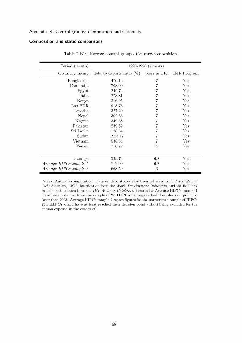
Appendix B. Control groups: composition and suitability.

Composition and static comparisons

Table 2.B1: Narrow control group - Country-composition.

Period (length) 1990-1996 (7 years)

Country name debt-to-exports ratio (%) years as LIC IMF Program

Bangladesh 476.16 7 YesCambodia 708.00 7 Yes

Egypt 249.74 7 YesIndia 273.81 7 Yes

Kenya 216.95 7 YesLao PDR 913.73 7 YesLesotho 327.29 7 YesNepal 302.66 7 Yes

Nigeria 349.38 7 YesPakistan 239.52 7 YesSri Lanka 178.64 7 Yes

Sudan 1925.17 7 YesVietnam 538.54 7 YesYemen 716.72 4 Yes

Average 529.74 6.8 YesAverage HIPCs sample 1 712.99 6.2 YesAverage HIPCs sample 2 668.59 6 Yes

Notes: Author’s computation. Data on debt stocks have been retrieved from InternationalDebt Statistics, LICs’ classification from the World Development Indicators, and the IMF pro-gram’s participation from the IMF Archives Catalogue. Figures for Average HIPCs sample 1have been obtained from the sample of 26 HIPCs having reached their decision point nolater than 2003. Average HIPCs sample 2 report figures for the unrestricted sample of HIPCs(34 HIPCs which have at least reached their decision point - Haiti being excluded for thereason exposed in the core text).

68

Table 2.B2: Extended control group countries.

Albania Dominican Republic Libya South AfricaAlgeria Ecuador Macedonia Sri LankaAngola Egypt Malaysia St. LuciaArgentina El Salvador Maldives St. VincentArmenia Equatorial Guinea Mauritius SudanAzerbaijan Eritrea Moldova SwazilandBangladesh Fiji Mongolia SyriaBelarus Georgia Morocco TajikistanBelize Grenada Myanmar ThailandBhutan Guatemala Nepal TongaBosnia and Herzegovina India Nicaragua TunisiaBotswana Indonesia Nigeria TurkeyBrazil Iran. Islamic Rep. Pakistan TurkmenistanBulgaria Jamaica Panama UkraineCambodia Jordan Papua New Guinea UzbekistanCape Verde Kazakhstan Paraguay VanuatuChina Kenya Peru VenezuelaColombia Kyrgyz Republic Philippines VietnamCosta Rica Lao PDR Romania YemenDjibouti Lebanon Samoa ZimbabweDominica Lesotho Serbia

African control group countriesLibya and Equatorial Guinea are excluded from the sample because of lack of data.

Notes: All countries considered for the extended and African control groups are countrieswhich have been ranked as a LIC at least once between 1990 and 1996.

69

Table 2.B3: Control groups and macro-covariates (average 1990-1996).

(I) (II) (III) (IV)

Control groups Difference before 1996

HIPC Narrow Extended African (I)-(II) (I)-(III) (I)-(IV)

Variables

Debt-to-exports 712.99 529.74 198.29 286.58 183.25*** 509.64*** 424.21***LIC Statuts 0.88 0.96 0.26 0.35 -0.08*** 0.61*** 0.53***Log GDP pc 5.98 6.14 7.26 7.07 -0.15*** -1.27*** -1.09***Openness rate 29.55 27.87 39.29 40.72 1.74 -9.69*** -11.14***Agriculture share 36.14 29.56 21.58 17.23 6.61*** 14.55*** 18.90***Resources share 10.88 10.98 8.19 9.33 -0.08 2.69*** 1.55***Log pop. Density 3.32 4.49 4.03 3.60 -1.17*** -0.71*** -0.28***Age dependency 94.08 86.17 75.16 85.85 7.91*** 18.91*** 8.22***Urban population 30.15 23.37 44.29 40.38 6.78*** -14.13*** -10.22***

Notes: In this table we observe macro-covariates average values for each group under review and over1990-1996 (which nearly coincides with the baseline period of HIPCs considered in sample 1). The HIPCgroup contains all HIPCs that have reached their decision point no later than 2003. Paired t-test areperformed in order to observe the difference in macro-covariates between HIPCs and countries includedin the different control groups (the narrow, extended, or African control group). We note, that althoughmost of the differences are statistically significant, differences with HIPCs are minimized (on average)when comparisons are performed with respect to narrow control group countries. ***, ** and * denotesignificance at 10%, 5% and 1%.

70

Parallel trend - Econometric analysis

The identification of treatment effects under the DID methodology is based on the hypothesis

of ex-ante parallel trends in the outcome variable between control and treated units. Consequently,

I run placebo tests to check for parallel trends in tax effort between HIPCs and the different

control groups before debt relief was granted. However, taking into account the potential

anticipatory effect over the years preceding the attainment of the decision point (captured by

β1 in equation 2.1), I investigate the parallel trend hypothesis before such anticipation takes

place, i.e. over the baseline period. Note that for 21 out of 26 HIPCs of our sample, the baseline

period corresponds to the years prior 1996, so before the HIPC initiative was officially disclosed.

In order to empirically observe the difference in tax effort evolution between HIPCs and

control group countries over the baseline, I run the following specification:

TEi,t = α+ δt + νHIPCi + βHIPCi ∗ Placeboi,t + ǫi,t (2.3)

where only observations over the baseline period for the HIPCs are considered, thus restricting

the time series for control group countries to 1999 (since for HIPCs having reached their decision

point in 2003, the baseline period ends in 1999). I then define Placeboi,t as a dummy variable

equal to 1 for the most recent half of the HIPCs’ respective baseline period. Note that the length

of the baseline period is HIPC-specific and depends on the date the HIPC reached its decision

point (date which varies between HIPCs). For instance, a country like Burkina Faso that reached

its decision point in 2000 will have its baseline period defined between 1990 and 1995 (with

the period running from 1996 to 1999 being the anticipatory phase). Therefore, the Placeboi,t

dummy is equal to 1 for years from 1993 to 1995 and 0 otherwise. For country having reached

their decision point in 2002 like Ghana, the baseline period runs from 1990 up to 1997 (with

the anticipatory phase over 1998-2001). In this case Placeboi,t is equal to 1 for the sub-period

1994-1997. In addition to this placebo treatment I include time-fixed effects as well as an HIPC

dummy to account for initial differences in tax effort with respect to the different control groups.

Alternately, I also consider a second specification to investigate the parallel trend hypothesis:

TEi,t = α+ δt + νHIPCi +−5∑

p=−8

βpHIPCi ∗DP (−p)i,t + ǫi,t (2.4)

where instead of splitting the baseline period in two, I observe the gradual evolution of tax

effort throughout this period and with respect to the first years of the baseline period (years

prior the year -8 as regards the decision point). The variable DP (−p)i,t is a dummy variable

equal to 1 in the year t corresponding to the year -p as regards the decision point of the HIPC i.

We thus have four dummy variables that capture the level of tax effort in HIPCs in -5, -6, -7,

and -8, and as compared with tax effort in older years. Any robust significance in these dummy

variable suggests a different trend in tax effort evolution between HIPCs and the control groups.

Results for both equation 2.3 and 2.4 are reported in Table 2.B4. Results denote an absence

of robust diverging path in tax effort between HIPCs and countries in the different control

groups. The Placebo coefficient is never significantly different from zero which therefore supports

the parallel trend hypothesis. The parallel trend hypothesis is also supported by even columns,

72

where dummy variables for the last four years of the HIPCs’ baseline period are not statistically

significant (except with respect to the extended control group, although the significance remains

marginal - at the 10% level).

Table 2.B4: Parallel trend analysis.

(I) (II) (III) (IV) (V) (VI)

Dep. var.: Tax effort index

Control group: Narrow Extended African

Placebo (ex-ante) -0.039 0.035 -0.028(-0.664) (0.848) (-0.512)

Placebo (year -5) 0.014 0.088* 0.019(0.130) (1.700) (0.255)

Placebo (year -6) -0.004 0.069* 0.021(-0.049) (1.658) (0.317)

Placebo (year -7) -0.053 0.020 -0.043(-0.799) (0.400) (-0.615)

Placebo (year -8) -0.010 0.051 0.014(-0.163) (0.745) (0.163)

HIPC Dummy -0.194*** -0.208*** -0.147*** -0.165*** -0.120*** -0.138***(-3.403) (-3.644) (-5.081) (-4.491) (-2.746) (-2.638)

Observations 289 289 813 813 319 319R-squared 0.641 0.643 0.428 0.429 0.608 0.610

Wald-Stat (p-value) 0.000 0.000 0.567 0.000 0.000 0.000No. of HIPCs 25 25 25 25 25 25

No. of control countries 14 14 78 78 17 17

Notes: Estimates have been obtained using the option vce(bootstrap) under STATA 13. Columns (I), (III),and (V) report estimate results of equation 2.3, while columns (II), (IV), and (VI) expose estimate results ofequation 2.4. Tax effort index measured at the country-year level are obtained from structural tax equation2.2 (column (1) in Table 2.A2, p.67). Tax effort estimates using specification 1 are quite large for Niger andcan thus rise doubts about the reliability of our results. We therefore removed Niger from our benchmarkestimates. Nevertheless, results with Niger do not change the conclusions and are available upon request tothe author. Robust z-statistics are exposed in parentheses. ***, ** and * denote significance at 10%, 5%and 1%. Results do not suggest an average significant divergence in tax effort evolution over thebaseline period between HIPCs and the various control groups, thus making them suitable forthe difference-in-differences analysis.

73

Appendix C. Robustness checks.

PANEL A - Debt-to-revenue ratio - (10 countries): Bangladesh, Cambodia, Kenya, Lao

PDR, Nepal, Nigeria, Sri Lanka, Sudan, Vietnam, Yemen.

PANEL B - IDA eligible - (37 countries): Albania, Angola, Armenia, Azerbaijan, Bangladesh,

Bhutan, Cape Verde, China, Djibouti, Egypt, Georgia, India, Indonesia, Kazakstan, Kenya,

Krygyz Republic, Lao PDR, Lesotho, Moldova, Mongolia, Morocco, Nepal, Nigeria, Pakistan,

Papua New Guinea, Philippines, Samoa, Sri Lanka, Sudan, Syria, Tajikistan, Turkmenistan,

Uzbekistan, Vanuatu, Vietnam, Yemen, Zimbabwe.

PANEL C - SIN and MIN - (21 countries): Argentina, Bangladesh, Brazil, Bulgaria,

Colombia, Dominican Republic, Ecuador, Guatemala, India, Indonesia, Kenya, Morocco, Myan-

mar, Nigeria, Pakistan, Peru, Philippines, Sudan, Syria, Turkey, Zimbabwe.

PANEL D - SIN only - (11 countries): Argentina, Brazil, Bulgaria, Ecuador, Kenya,

Morocco, Myanmar, Nigeria, Peru, Sudan, Syria.

Note that countries are defined as severely indebted (SIN) and moderatly indebted (MIN)

following the World bank’s definition: “Severely indebted means either: PV of debt service to

GNI exceeds 80 percent or PV of debt service to exports exceeds 220 percent. Moderately indebted

means either of the two key ratios exceeds 60 percent of, but does not reach, the critical levels.

For economies that do not report detailed debt statistics to the World Bank Debtor Reporting

System (DRS), PV calculation is not possible. Instead, the following methodology is used to

classify the non-DRS economies. Severely indebted means three of four key ratios (averaged over

three years) are above critical levels: debt to GNI (50 percent); debt to exports (275 percent);

debt service to exports (30 percent); and interest to exports (20 percent). Moderately indebted

means three of the four key ratios exceed 60 percent of, but do not reach, the critical levels. All

other classified low income and middle-income economies are listed as less indebted”.

PSM-based control groups

As explained in the core text, I specify a Probit model where the probability of being HIPC

under the Enhanced HIPC initiative (regardless the date of debt relief provision) is determined

by covariates averaged over 1990-1996. This model can thus be written as follows:

Pr(HIPCi) = Φ(DEBTi,90−96, GNI PCi,90−96, EXPORTSi,90−96, IMPORTSi,90−96,

AGRIi,90−96, NAT RESi,90−96, POP DENSi,90−96, ODAi,90−96,

POLITY IVi,90−96, TAX EFFORTi,90−96)

where HIPCi is a dummy variable equal to 1 if the country i has been granted debt relief

under the Enhanced HIPC over our entire period of study (so between 1990 and 2012). Then,

the covariates that could potentially explain why some countries have benefited from this initia-

tive (out of the 113 countries of our sample) are averaged over 1990-1996, so before the first

HIPC initiative was disclosed. DEBTi,90−96 is the average debt-to-exports ratio over 1990-1996,

GNI PCi,90−96 the average GNI per capita (using World Bank Atlas methodology on which IDA

eligibility is based), EXPORTSi,90−96 and IMPORTSi,90−96 then denote exports and imports’

74

average shares into the GDP over 1990-1996, AGRIi,90−96 is the average share of GDP accruing

to the agricultural sector, NAT RESi,90−96 is the average natural resource rents (also expressed

in GDP percentage), POP DENSi,90−96 is the average log of population density (averaged over

1990-1996). Then, ODAi,90−96 denotes as before the average ODA grants received between 1990

and 1996 (net of debt relief grants) and expressed in percentage of GDP. POLITY IVi,90−96

defines the institutional quality and ranks countries from autocracy to democracy. Lastly,

TAX EFFORTi,90−96 is the average level of tax effort over 1990-1996 (derived from column (1)

specification of Table 2.A2, p.67) which captures most of the baseline period for HIPCs that

have reached their decision point in the early 2000s.

Table 2.C1 below exposes results of Probit estimates. Results of the different Probit model

show that, in keeping with the design of the Enhanced HIPC initiative and the eligibility criteria,

more indebted and poorer countries (between 1990 and 1996) are more likely to benefit from this

initiative. One can also note that exporting countries expose higher probability of being selected

into the program, and that countries which are more imports-oriented are less likely to join the

initiative. In addition, results suggest that non-resource rich countries and those receiving more

ODA are more likely to benefit from these debt relief initiatives. Lastly, the average level of tax

effort before 1996 is also found as being an important determinant of the HIPC status. Countries

with lower average level of tax effort, indeed report a greater probability of being selected as an

HIPC. Interestingly, and in keeping with Presbitero (2009) and Freytag and Pehnelt (2009), we

note that institutional quality (here proxied by the Polity IV autocracy/democracy index) plays

a positive role in the participation of these debt relief programs.

From Table 2.C1, I derive three propensity scores, each stemming from a particular Probit

specification. Some countries have their propensity score computed in each Probit specification,

but some other do not, due to missing values on ex-ante economic covariates. Therefore, the

number of countries included in the control group can vary according to the specification I used

to derived propensity scores, and the propensity score threshold above which countries have

to satisfied for being considered as a counterfactual. Countries reported below are countries

with a propensity score above 0.2 in Panel F, and with propensity score above 0.5 in Panel G.

Countries in bold font have their propensity score calculated for each specification and above

the required threshold in each situation (so regardless the Probit specification). Countries in

italic font have propensity scores above the threshold for only two Probit specifications. Lastly,

countries in normal font breach the propensity score threshold when their propensity score have

been calculated with only one Probit specification.

Propensity score ≥ 0.2: Angola, Armenia, Azerbaijan, Bangladesh, Bhutan, Cape Verde,

Djibouti, China, Eritrea, Georgia, India, Kenya, Kyrgyz Republic, Lao PDR, Lesotho,

Moldova, Nepal, Nigeria, Pakistan, Papua New Guinea, Samoa, Sudan, Tajikistan, Turk-

menistan, Vietnam, Yemen.

Propensity score ≥ 0.5: Angola, Bangladesh, Bhutan, Djibouti, Georgia, Kenya, Kyrgyz

Republic, Lao PDR, Lesotho, Nepal, Samoa, Sudan, Tajikistan, Turkmenistan, Vietnam.

75

Table 2.C1: Propensity score estimates.

Probit specification: (1) (2) (3)

Dep. var.: HIPCi

(1 if HIPC - 0 otherwise)

av. DEBTi,90−96 0.001** 0.001** 0.001(2.304) (2.501) (0.955)

av. GNI PCi,90−96 -0.002*** -0.002** -0.003**(-2.775) (-2.490) (-2.129)

av. EXPORTSi,90−96 0.034* 0.212***(1.677) (3.030)

av. IMPORTSi,90−96 -0.023 -0.196***(-1.503) (-3.091)

av. AGRIi,90−96 -0.002 0.030(-0.092) (1.186)

av. NAT RESi,90−96 -0.022 -0.082***(-1.227) (-2.629)

av. POP DENSi,90−96 -0.237(-0.941)

av. ODAi,90−96 0.317***(3.373)

av. POLITY IVi,90−96 0.139**(2.232)

av. TAX EFFORTi,90−96 -2.364** -2.812*** -2.950*(-2.449) (-2.648) (-1.888)

Constant 2.601*** 3.290** 3.453(2.658) (2.136) (1.449)

Observations 103 103 96Prob ≥ Chi2 0.000 0.000 0.000Pseudo R2 0.432 0.464 0.671

Notes: Probit estimates mobilize observations at the country-level (oneobservation per country). The dependent variable (HIPCi) is equalto 1 for countries defined as HIPC, 0 otherwise. The explanatoryvariables are average values of macro-covariates over 1990-1996. Welose 7 countries for column (3) estimate because of missing values in thePOLITY IV variable. ***, ** and * denote significance at 10%, 5%and 1%.

76

Table 2.C2: Differences in ex-ante covariates - HIPCs vs propensity score-based control groups.

(I) (II) (III) (IV) (V) (VI) (VII)

Propensity score ≥ 0.2 Propensity score ≥ 0.5

HIPCs C1 C1 - HIPC C2 C2 - HIPC

Mean Mean Diff. p.val Mean Diff p.valProbit specification 1

av. DEBTi,90−96 712.99 318.13 -444.58 0.005*** 601.34 -111.64 0.693av. GNI PCi,90−96 361.18 419.44 58.26 0.259 378.57 17.39 0.820

av. TAX EFFORTi,90−96 0.91 0.99 0.07 0.177 0.90 -0.01 0.852Propensity scorei 0.65 0.45 -0.20 0.002*** 0.66 0.01 0.896

Observations 26 23 - - 8 - -

Probit specification 2

av. DEBTi,90−96 712.99 343.57 -369.42 0.078* 463.02 -249.97 0.336av. GNI PCi,90−96 361.18 404.19 43.01 0.447 369.82 8.64 0.900

av. EXPORTSi,90−96 23.99 30.25 6.26 0.298 32.49 8.49 0.248av. IMPORTSi,90−96 35.10 35.42 0.32 0.956 39.23 4.12 0.563

av. AGRIi,90−96 36.02 33.03 -2.98 0.426 35.62 -0.39 0.932av. NAT RESi,90−96 10.88 10.97 0.09 0.976 12.31 1.43 0.697

av. TAX EFFORTi,90−96 0.91 0.96 0.05 0.367 0.92 0.01 0.921Propensity scorei 0.67 0.54 -0.13 0.049** 0.65 -0.02 0.741

Observations 26 16 - - 10 - -

Probit specification 3

av. DEBTi,90−96 712.99 394.31 -318.68 0.182 422.79 -290.19 0.345av. GNI PCi,90−96 361.18 440.88 79.69 0.267 506.93 145.75 0.111

av. EXPORTSi,90−96 23.99 29.93 5.93 0.363 34.45 10.45 0.200av. IMPORTSi,90−96 35.10 35.72 0.61 0.926 39.68 4.57 0.579

av. AGRIi,90−96 36.02 31.42 -4.59 0.306 27.85 -8.16 0.139av. NAT RESi,90−96 10.88 12.44 1.56 0.652 18.50 7.62 0.069*

av. POP DENSi,90−96 3.32 3.79 0.47 0.288 3.07 -0.25 0.608av. ODAi,90−96 13.02 7.38 -5.63 0.053* 10.47 -2.54 0.477

av. POLITY IVi,90−96 -0.42 -1.33 -0.91 0.620 -3.24 -2.82 0.180av. TAX EFFORTi,90−96 0.91 1.03 0.11 0.039** 0.99 0.08 0.275

Propensity scorei 0.81 0.48 -0.33 0.000*** 0.63 -0.18 0.059*

Observations 26 12 - - 7 - -

Notes: The HIPCs sample is made up of 26 countries having reached their decision point no later than2003. C1 (control group 1) considers non-HIPCs with a propensity score above 0.2, while C2 limits thegroup to non-HIPCs with a propensity score superior to 0.5. The Table also reports the difference (as wellas the statistical significance of this difference) in covariates’ mean value before 1996, and between HIPCsand the two control groups. ***, ** and * denote significance at 10%, 5% and 1%.

77

Alternative dependent variables

Table 2.C3: Tax effort index - Pairwise correlation matrix.

Models: (1) (2) (3) (4)

(1) 1.000(2) 0.915 1.000(3) 0.826 0.834 1.000(4) 0.381 0.430 0.456 1.000

Notes: Pairwise correlations are all statisti-cally significant at the 1% level. Models (1),(2), (3), (4) correspond to estimate resultsfrom columns (1), (2), (3), and (4) respec-tively (cf. Table 2.A2 in the Appendix A,p.67).

Table 2.C4: ICTD Disaggregated taxes & data coverage - 113 Developing Countries [1990-2012]

Variables (in % of GDP) Mean Std. Dev. Obs. % missing

Total non-resource taxes 14.13 6.55 2407 8.99

Indirect taxes 9.77 4.89 2115 20.03of which Taxes on goods and services 6.02 3.59 2113 20.11of which Taxes on international trade 3.41 3.74 2096 20.75

Direct taxes 4.46 2.95 2148 18.79of which Taxes on income 1.85 1.75 1565 40.83

of which Taxes on profits gains 2.32 1.92 1535 41.96

Notes: Data come from the GRD (ICTD) (Prichard et al., 2014). December 2015 database availableon the UNU-WIDER website

78

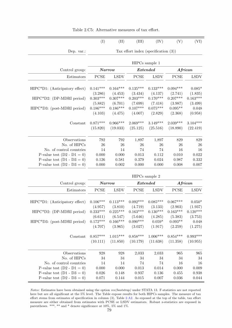
Table 2.C5: Alternative measures of tax effort.

(I) (II) (III) (IV) (V) (VI)

Dep. var.: Tax effort index (specification (3))

HIPCs sample 1

Control group: Narrow Extended African

Estimators PCSE LSDV PCSE LSDV PCSE LSDV

HIPC*D1: (Anticipatory effect) 0.141*** 0.164*** 0.135*** 0.133*** 0.094*** 0.085*(3.286) (4.453) (3.434) (4.137) (2.741) (1.835)

HIPC*D2: (DP-MDRI period) 0.303*** 0.307*** 0.203*** 0.170*** 0.207*** 0.163***(5.882) (6.701) (7.699) (7.418) (3.987) (3.499)

HIPC*D3: (post-MDRI period) 0.186*** 0.186*** 0.107*** 0.075*** 0.095** 0.048(4.103) (4.475) (4.007) (2.829) (2.368) (0.958)

Constant 0.871*** 0.966*** 2.069*** 3.149*** 2.039*** 3.104***(15.820) (19.033) (25.125) (25.516) (18.890) (22.419)

Observations 792 792 1,897 1,897 829 829No. of HIPCs 26 26 26 26 26 26

No. of control countries 14 14 74 74 16 16P-value test (D2 - D1 = 0) 0.000 0.000 0.013 0.112 0.010 0.022P-value test (D1 - D3 = 0) 0.126 0.581 0.379 0.024 0.987 0.332P-value test (D2 - D3 = 0) 0.000 0.002 0.000 0.000 0.008 0.007

HIPCs sample 2

Control group: Narrow Extended African

Estimators PCSE LSDV PCSE LSDV PCSE LSDV

HIPC*D1: (Anticipatory effect) 0.106*** 0.113*** 0.092*** 0.085*** 0.067*** 0.050*(4.957) (3.810) (4.719) (3.133) (2.903) (1.937)

HIPC*D2: (DP-MDRI period) 0.233*** 0.225*** 0.163*** 0.130*** 0.163*** 0.120***(6.611) (6.547) (5.646) (4.285) (5.383) (3.753)

HIPC*D3: (post-MDRI period) 0.172*** 0.166*** 0.090*** 0.059* 0.093** 0.048(4.707) (3.965) (3.027) (1.917) (2.259) (1.275)

Constant 0.857*** 1.015*** 0.858*** 1.006*** 0.854*** 0.993***(10.111) (11.850) (10.179) (11.638) (11.358) (10.955)

Observations 928 928 2,033 2,033 965 965No. of HIPCs 34 34 34 34 34 34

No. of control countries 14 14 74 74 16 16P-value test (D2 - D1 = 0) 0.000 0.000 0.013 0.014 0.000 0.009P-value test (D1 - D3 = 0) 0.026 0.148 0.937 0.136 0.455 0.938P-value test (D2 - D3 = 0) 0.071 0.144 0.015 0.007 0.036 0.044

Notes: Estimates have been obtained using the option vce(bootstrap) under STATA 13. F-statistics are not reportedhere but are all significant at the 5% level. The Table expose results for both HIPCs samples. The measure of taxeffort stems from estimates of specification in column (3), Table 2.A2. As exposed at the top of the table, tax effortmeasure are either obtained from estimates with PCSE or LSDV estimators. Robust z-statistics are exposed inparentheses. ***, ** and * denote significance at 10%, 5% and 1%.

79

Appendix D. Moral hazard around the MDRI - additional results.

Table 2.D1: Descriptive statistics on political instability.

Over the entire period

For HIPCs sample 1 Mean Sd Min Max % missing

Political Instability 0.49 0.74 -1.04 2.98 39%Political Instability II 0.50 0.76 -1.04 2.98 26%

Inverted regime durability -9.71 9.14 -42 0 4%Years Left in current term 2.25 1.58 0 6 17%

For non-HIPCs

Political Instability 0.40 0.85 -1.41 2.80 39%Political Instability II 0.40 0.85 -1.41 2.80 26%

Inverted regime durability -17.11 18.59 -97 0 13%Years Left in current term 2.05 1.46 0 6 20%

Post-baseline (after 1996 for CG countries)

For HIPCs sample 1 Mean Sd Min Max % missing

Political Instability 0.47 0.72 -1.04 2.58 17%Political Instability II 0.47 0.73 -1.04 2.78 0%

Inverted regime durability -9.42 8.05 -42 0 4%Years Left in current term 2.19 1.56 0 6 12%

For non-HIPCs

Political Instability 0.40 0.85 -1.41 2.80 18%Political Instability II 0.40 0.85 -1.41 2.80 1%

Inverted regime durability -18.14 18.69 -97 0 13%Years Left in current term 2.02 1.45 0 6 18%

Notes: Political Instability is the WGI (KKZ) measure of political stability andabsence of violence which has been multiplied by -1. Political Instability II is thesame variable where missing values for 1997, 1999, and 2001 have been filled up usingTaylor-Young linear approximation. Inverted regime durability comes from the PolityIV dataset and multiplies by -1 the number of years since the last policy regimechange. Therefore increase in this variable denotes shorter period since the last regimechange. Lastly, Years left in current term come from the Dataset on PoliticalInsitutions (DPI).

80

Table 2.D2: Debt relief and tax effort - control for government’s preference for present.

(I) (II) (III) (IV) (V) (VI) (VII) (VIII) (IX) (X) (XI) (XII)

Dep. var.: Tax effort index

Control Group Narrow Extended African

HIPCs sample 1

HIPC*D2: (DP-MDRI period) 0.168** 0.155*** 0.169*** 0.115*** 0.087** 0.074** 0.082** 0.035 0.125** 0.110*** 0.110*** 0.041(2.447) (3.830) (4.677) (3.318) (2.279) (2.516) (2.524) (1.254) (2.086) (2.736) (2.662) (0.963)

HIPC*D3: (post-MDRI period) 0.040 0.016 0.033 0.044 -0.001 -0.020 -0.003 -0.037 0.026 -0.003 -0.001 -0.022(0.694) (0.379) (0.982) (1.051) (-0.038) (-0.767) (-0.114) (-1.492) (0.468) (-0.078) (-0.037) (-0.501)

Political Instability -0.053** -0.033** -0.043(-2.316) (-2.155) (-1.563)

Political Instability II -0.062*** -0.041*** -0.060**(-2.670) (-2.920) (-2.530)

Inverted regime durability 0.000 -0.001** -0.002*(0.119) (-2.001) (-1.715)

Years left in current term 0.009** 0.006** 0.009*(2.067) (2.466) (1.695)

Constant 1.024*** 1.041*** 0.946*** 1.066*** 0.940*** 0.960*** 0.955*** 0.914*** 0.980*** 1.011*** 0.828*** 0.890***(13.095) (20.855) (11.142) (12.151) (8.489) (10.417) (9.638) (13.735) (8.530) (8.778) (8.023) (9.075)

Observations 507 621 694 616 1,315 1,608 1,813 1,675 542 665 755 622R-squared 0.284 0.253 0.216 0.327 0.266 0.237 0.094 0.150 0.236 0.210 0.170 0.237

Notes: Estimates have been obtained using the option vce(bootstrap) under STATA 13. F-statistics are not reported here but are all significant at the 5% level. The Table exposes results for HIPCssample 1 since it includes HIPCs with the longer post-MDRI period (7 years for all of them). Note that running estimates with HIPCs sample 2 gives the same results (available upon request tothe author). The study period has been shortened by dropping observations before 1996 which corresponds to the baseline of most HIPCs of this sample. Therefore, the reference period forHIPCs to which coefficients HIPC ∗D2 and HIPC ∗D3 must be compared with is the anticipatory phase. Absence of statistical significance for HIPC ∗D2 and HIPC ∗D3 suggestsno different level of tax effort in the extended interim and post-MDRI periods as regards the level recorded during the anticipatory period. Tax effort index measured at thecountry-year level are obtained from structural tax equation 2.2 (column (1) in Table 2.A2, P.67). Robust z-statistics are exposed in parentheses. ***, ** and * denote significance at 10%, 5% and 1%.

81

Table 2.D3: Do conflicts explain changes in tax effort around debt relief?

Dep. var.: Tax effort index

HIPCs sample 1 HIPCs sample 2

Control Group: Narrow Extended African Narrow Extended African

HIPC*D1: (Anticipatory effect) 0.193*** 0.194*** 0.146*** 0.146*** 0.137*** 0.138*** 0.144*** 0.144*** 0.108*** 0.108*** 0.100*** 0.101***(5.213) (4.752) (5.371) (4.587) (3.760) (3.090) (5.959) (4.535) (5.130) (3.781) (4.276) (3.805)

HIPC*D2: (DP-MDRI period) 0.353*** 0.353*** 0.221*** 0.221*** 0.239*** 0.240*** 0.268*** 0.269*** 0.187*** 0.188*** 0.192*** 0.193***(7.574) (7.502) (8.706) (7.712) (6.278) (5.778) (8.395) (6.204) (8.196) (6.849) (6.642) (5.652)

HIPC*D3: (post-MDRI period) 0.183*** 0.181*** 0.110*** 0.110*** 0.092** 0.093** 0.161*** 0.161*** 0.097*** 0.096*** 0.086*** 0.086**(3.847) (4.114) (3.816) (3.607) (2.291) (2.154) (3.957) (4.164) (4.236) (3.356) (2.634) (2.523)

Conflicts -0.002 -0.017 0.004 0.013 -0.007 0.024(-0.140) (-1.365) (0.137) (0.812) (-0.449) (1.082)

Interstate conflicts 0.063 0.047 0.007 0.034 0.039 0.001(1.311) (1.364) (0.176) (0.833) (1.022) (0.017)

Internal conflicts -0.009 -0.022 0.002 0.010 -0.012 0.023(-0.544) (-1.581) (0.056) (0.485) (-0.989) (0.910)

Internationalized conflicts -0.003 -0.017 0.012 0.022 0.002 0.031(-0.049) (-0.361) (0.180) (0.397) (0.040) (0.762)

Constant 0.811*** 0.811*** 0.945*** 0.944*** 0.885*** 0.886*** 0.608*** 0.598*** 0.665*** 0.656*** 0.587*** 0.580***(13.360) (15.135) (19.014) (11.591) (9.968) (11.278) (6.559) (5.867) (8.319) (8.047) (6.963) (5.566)

Observations 854 854 2,135 2,135 916 916 1,008 1,008 2,289 2,289 1,070 1,070R-squared 0.166 0.167 0.087 0.088 0.129 0.129 0.139 0.139 0.083 0.084 0.115 0.115

P-value test (D2 - D1 = 0) 0.000 0.000 0.008 0.001 0.002 0.000 0.000 0.000 0.012 0.000 0.000 0.000P-value test (D1 - D3 = 0) 0.814 0.748 0.150 0.222 0.219 0.210 0.592 0.621 0.701 0.606 0.631 0.616P-value test (D2 - D3 = 0) 0.000 0.000 0.000 0.000 0.000 0.000 0.002 0.006 0.002 0.000 0.003 0.000

Notes: Estimates have been obtained using the option vce(bootstrap) under STATA 13. F-statistics are not reported here but are all significant at the 5% level. The Table exposes results for HIPCssamples 1 and 2. Data on conflicts come from the latest version of the UCDP/PRIO Armed Conflict Dataset (Gleditsch et al., 2002; Harbom and Wallensteen, 2010). Tax effort index measuredat the country-year level are obtained from structural tax equation 2.2 (column (1) in Table 2.A2, p.67). Robust z-statistics are exposed in parentheses. ***, ** and * denote significance at 10%, 5%and 1%.

82

Table 2.D4: Pairwise correlation between measures of government quality.

GOV.EF REG.Q GOV.Q CPIA

(WGI) GOV.EF 1.000(.)

(WGI) REG.Q 0.877 1.000(0.000) (.)

(ICRG) GOV.Q 0.592 0.524 1.000(0.000) (0.000) (.)

(IRAI) CPIA 0.782 0.805 0.453 1.000(0.000) (0.000) (0.000) (.)

Notes: This table reports the pairwise correlation between our differentmeasures (averaged over 2004-2005) of institutional quality for the entiresample. GOV.EF denotes government effectiveness as measured by theWGI-KKZ methodology. REG.Q represents regulatory quality andalso comes from the WGI dataset. GOV.Q is the government qualitymeasured by the ICRG. Lastly, CPIA is the classic indicator provided bythe World Bank and used by the IDA for its resource allocation criteria.P-values of the pairwise correlation between the different indicators arereported in brackets below correlation coefficients.

83

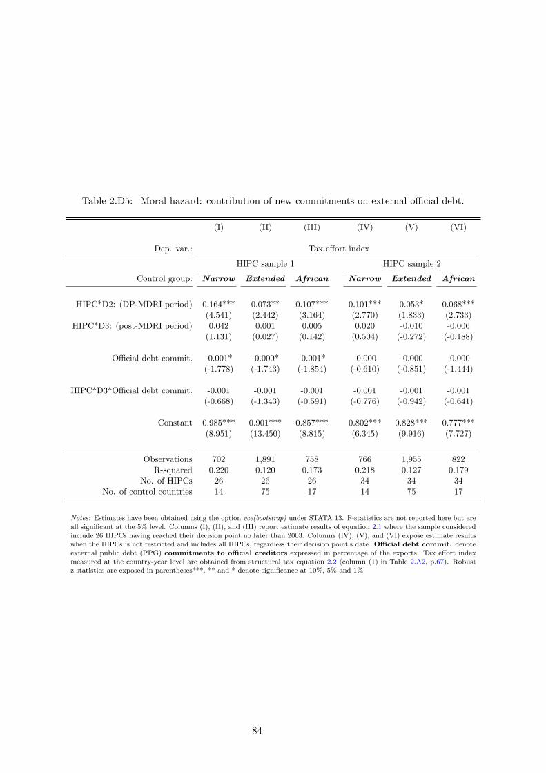
Table 2.D5: Moral hazard: contribution of new commitments on external official debt.

(I) (II) (III) (IV) (V) (VI)

Dep. var.: Tax effort index

HIPC sample 1 HIPC sample 2

Control group: Narrow Extended African Narrow Extended African

HIPC*D2: (DP-MDRI period) 0.164*** 0.073** 0.107*** 0.101*** 0.053* 0.068***(4.541) (2.442) (3.164) (2.770) (1.833) (2.733)

HIPC*D3: (post-MDRI period) 0.042 0.001 0.005 0.020 -0.010 -0.006(1.131) (0.027) (0.142) (0.504) (-0.272) (-0.188)

Official debt commit. -0.001* -0.000* -0.001* -0.000 -0.000 -0.000(-1.778) (-1.743) (-1.854) (-0.610) (-0.851) (-1.444)

HIPC*D3*Official debt commit. -0.001 -0.001 -0.001 -0.001 -0.001 -0.001(-0.668) (-1.343) (-0.591) (-0.776) (-0.942) (-0.641)

Constant 0.985*** 0.901*** 0.857*** 0.802*** 0.828*** 0.777***(8.951) (13.450) (8.815) (6.345) (9.916) (7.727)

Observations 702 1,891 758 766 1,955 822R-squared 0.220 0.120 0.173 0.218 0.127 0.179

No. of HIPCs 26 26 26 34 34 34No. of control countries 14 75 17 14 75 17

Notes: Estimates have been obtained using the option vce(bootstrap) under STATA 13. F-statistics are not reported here but areall significant at the 5% level. Columns (I), (II), and (III) report estimate results of equation 2.1 where the sample consideredinclude 26 HIPCs having reached their decision point no later than 2003. Columns (IV), (V), and (VI) expose estimate resultswhen the HIPCs is not restricted and includes all HIPCs, regardless their decision point’s date. Official debt commit. denoteexternal public debt (PPG) commitments to official creditors expressed in percentage of the exports. Tax effort indexmeasured at the country-year level are obtained from structural tax equation 2.2 (column (1) in Table 2.A2, p.67). Robustz-statistics are exposed in parentheses***, ** and * denote significance at 10%, 5% and 1%.

84

Table 2.D6: Moral hazard: contribution of new commitments to external private creditors.

(I) (II) (III) (IV) (V) (VI)

Dep. var.: Tax effort index

HIPC sample 1 HIPC sample 2

Control group: Narrow Extended African Narrow Extended African

HIPC*D2: (DP-MDRI period) 0.176*** 0.053** 0.073** 0.109*** 0.053*** 0.073**(4.105) (2.283) (2.022) (3.731) (2.597) (2.512)

HIPC*D3: (post-MDRI period) 0.048 -0.021 -0.008 0.017 -0.021 -0.008(1.441) (-0.864) (-0.190) (0.471) (-1.074) (-0.200)

Debt commit. to priv. -0.007*** 0.001 0.000 -0.007*** 0.001 0.000(-2.848) (1.271) (0.042) (-2.903) (1.327) (0.049)

HIPC*D3*Debt commit. to priv. 0.003 -0.005 -0.004 0.003 -0.005 -0.004(0.364) (-0.967) (-0.706) (0.427) (-0.837) (-0.764)

Constant 0.962*** 0.826*** 0.767*** 0.807*** 0.826*** 0.767***(10.585) (8.977) (6.247) (7.105) (11.077) (7.620)

Observations 702 1,955 822 766 1,955 822R-squared 0.233 0.129 0.179 0.234 0.129 0.179

No. of HIPCs 26 26 26 34 34 34No. of control countries 14 75 17 14 75 17

Notes: Estimates have been obtained using the option vce(bootstrap) under STATA 13. F-statistics are not reported here but areall significant at the 5% level. Columns (I), (II), and (III) report estimate results of equation 2.1 where the sample consideredinclude 26 HIPCs having reached their decision point no later than 2003. Columns (IV), (V), and (VI) expose estimate results ofequation 2.1 when the HIPCs is not restricted and includes all HIPCs, regardless their decision point’s date. Debt commit. topriv. denote external public debt (PPG) commitments to private creditors expressed in percentage of the exports. Taxeffort index measured at the country-year level are obtained from structural tax equation (1) (column (1) in Table 2.A2, p.67).Robust z-statistics are exposed in parentheses***, ** and * denote significance at 10%, 5% and 1%.

85

Appendix E. Miscellaneous.

Benchmark results including Niger

Table 2.E1: Benchmark results - including Niger.

(I) (II) (III) (IV) (V) (VI)

Dep. var.: Tax effort index

HIPC sample 1 HIPC sample 2

Control group: Narrow Extended African Narrow Extended African

HIPC*D1: (Anticipatory effect) 0.195*** 0.150*** 0.139*** 0.144*** 0.112*** 0.101***(4.601) (4.659) (3.439) (5.364) (3.716) (3.416)

HIPC*D2: (DP-MDRI period) 0.367*** 0.236*** 0.253*** 0.276*** 0.200*** 0.200***(7.574) (6.964) (6.500) (7.088) (7.312) (7.071)

HIPC*D3: (post-MDRI period) 0.250*** 0.177*** 0.159*** 0.218*** 0.156*** 0.143***(4.978) (5.215) (3.173) (4.848) (5.665) (3.287)

Constant 0.786*** 0.942*** 0.884*** 0.602*** 0.636*** 0.591***(13.224) (13.065) (10.378) (6.637) (5.993) (5.979)

Observations 877 2,158 939 1,031 2,312 1,093No. of HIPCs 27 27 27 35 35 35

No. of control countries 14 78 17 14 78 17Country fixed effects Yes Yes Yes Yes Yes Yes

Time fixed effects Yes Yes Yes Yes Yes YesR-squared 0.276 0.164 0.248 0.245 0.157 0.227

Test: D2 - D1 = 0 (p-val.) 0.000 0.000 0.000 0.000 0.000 0.000Test: D1 - D3 = 0 (p-val.) 0.231 0.246 0.645 0.058 0.152 0.310Test: D2 - D3 = 0 (p-val.) 0.023 0.022 0.021 0.215 0.105 0.121

Notes: Estimates have been obtained using the option vce(bootstrap) under STATA 13. F-statistics are not reported here but areall significant at the 5% level. Columns (I), (II), and (III) report estimate results of equation 2.1 where the sample consideredinclude 26 HIPCs having reached their decision point no later than 2003. Columns (IV), (V), and (VI) expose estimate results ofequation 2.1 when the HIPCs sample is not restricted and includes all HIPCs, regardless their decision point’s date. Tax effortindex measured at the country-year level are obtained from structural tax equation 2.2 (column (1) in Table 2.A2, p.67). Robustz-statistics are exposed in parentheses. ***, ** and * denote significance at 10%, 5% and 1%.

Parallel trend - Graphical analysis

Average evolution of tax-to-GDP ratios and tax effort index for HIPCs and control groups

around the decision point have been obtained as follows:

For the sample of HIPCs that have reached their decision point no later than 2003, figures for

each year regarding the year of the decision point’s attainment (-9, -8, ..., 0, 1, ..., 9) represent

the average tax effort performance of HIPCs in that given year. For instance, for the year ”0”

(the year where decision point has been reached) we calculate the average tax effort (A TAX E)

in 2000 (over 21 HIPCs having reached the decision point in 2000), the A TAX E in 2001 (over 2

HIPCs having reached their decision point in 2001), the A TAX E in 2002 (over 2 HIPCs having

reached their decision point in 2002), and the A TAX E in 2003 (which consists in the 2003

tax effort of Democratic Republic of Congo (DRC), since only DRC reached its decision point

86

in that year). We multiply each of these average figures by the number of HIPCs that have

been used to compute the mean, then sum these weighted average figures, and lastly divide this

sum by 26 (the number of HIPCs having reached their decision point no later than 2003). This

allows to give more weight to the A TAX E calculated for 2000 since it has been obtained over

21 HIPCs. Replicating this for every year in the range [-9; +9] as regards the decision point, we

thus get a unique series of weighted average tax effort for our sample of 26 HIPCs (the solid

black line in the graphs).

The calculation of the A TAX E for the different control groups follows the same philosophy.

But, instead of computing average tax effort in 2000 over HIPCs, we just compute average tax

effort in 2000 over countries included in the narrow control group (or extend/African control

groups for the two other series). Once the average values computed for the four different

“decision-point regimes” (2000, 2001, 2002, 2003), we again multiply by the number of HIPCs in

the relative decision-point regime, sum these values and divide the sum by 26. As for the HIPC

series, replicating this for every year in the range [-9; +9] as regards the decision point provides

a unique series of weighted average tax effort for the different control groups (the solid gray

lines in the graphs).

Table 2.E2 below provides an example of a simple hand calculation for the narrow control

group’s series of tax effort. The resulting weighted average tax effort for this control group is

then plotted in the Figure 2.E1. One can easily notice that it is the same series as the one

observed in Figure 2.4 (the solid gray line, p.46).

87

Chapter 3

Low Income Countries and External Public

Financing: Does Debt Relief Change

Anything?

with Marc Raffinot and Baptiste Venet

3.1 Introduction

Many low income countries (LICs) have been granted debt relief by bilateral creditors and

international financial institutions under the HIPC (Heavily Indebted Poor Countries) initiatives

since 1996, and the MDRI (Multilateral Debt Relief Initiative) since 2005. How have these debt

relief initiatives impacted on HIPC financing? Have they led creditors to change their lending

policies, deterring them from continuing to lend to LICs or prompting them to change their

conditions? This paper sets out to answer these questions with an empirical assessment of the

impact of debt relief on the financing conditions attached to official lending. We also investigate

whether these initiatives have helped beneficiary countries access new financing sources such as

international financial markets, and try to identify the circumstances under which this might

have happened.

Historically, Rawling’s Ghana refused HIPC debt relief in the first place, because of fears

of subsequent increases in interest rates (although it was the only HIPC country to do so).

The same concern lay behind the refusal of Sri Lanka, Indonesia and India to have their debt

rescheduled following the tsunamis. Yet can the increase in risk premium and the narrowing of

financing opportunities be deemed rational following a debt cancellation? In actual fact, debt

relief probably sends a mixed signal. On the one hand, debt relief would not be expected to

build confidence because countries unable to repay their debt in the past could be seen as risky

borrowers. On the other hand, debt relief improves debt sustainability by creating fiscal space.

The surge in bond issues by African countries on the international financial markets appears

to provide the answer: investors like countries without debt. In addition, the global economic

turmoil of recent years has prompted investors to search for assets with higher returns, such

as African bonds. In 2011, Graham Stock, Director of JP Morgan’s Research Department on

89

Emerging Countries, explained that the increase in commodity prices, high Chinese demand,

and the growing quality of institutions on the continent was improving the appeal of African

bonds to investors seeking portfolio diversification with attractive returns.1 He went on to say

that the debt relief initiatives had really improved debt sustainability in those countries as they

had reassured investors about the debtor’s capacity to pay in the short and medium term.2

However, the story is not that straightforward since some bond-issuing countries were not

LICs or HIPCs (Kenya and Gabon). The surge might then be due to the “irrational exuberance

of the markets” in a situation of historically low interest rates in OECD countries. This increase

could also be explained by Africa’s improving economic prospects attracting new financing from

emerging countries, in particular China, India and Brazil. Yet some other countries that were

HIPCs, such as Ghana and Senegal, appear to have problems borrowing regularly and steadily.

In addition, the high interest rates charged by private lenders have raised concerns that loans to

Africa might be no other than a new wave of “subprime loans” (Stiglitz and Rashid, 2013).

Bear in mind, however, that even after debt relief, the majority of LIC and HIPC financing

remains official (public) financing. As shown by Figure 3.1 below, bilateral and multilateral

loans account for nearly all external public debt disbursements in LICs. And although public

financing institutions switched, at least partly, from loans to grants after the 1982 debt crisis,

this trend has been reversing since 2006 due to commitments to increase Official Development

Aid (ODA) in a situation of public finance crisis in the donor countries.

Figure 3.1: Evolution of external public debt in LICs.

Sources: International Debt Statistics Database - World Databank, downloaded on the 12/21/2016.

1With spreads on African bonds 400 to 600 basis points higher than on European bonds.2Les Afriques, No. 167, 23 to 29 June, 2011.

90

So it is likely that bilateral creditors, who already agreed to cancel a significant part of

the claims they had on HIPCs, are now looking for higher (than before) returns on new loans and

are tightening their financing conditions by lowering the level of concessionality. However, such

a shift would be less expected from multilateral donors given the rigidity of their lending policy,

which remains mostly defined by economic and institutional features of recipient countries.

We use a difference-in-differences (DID) methodology to first investigate whether debt relief

provided under the Enhanced HIPC initiative and the MDRI has led official donors to change

the lending terms they offer to beneficiary countries. We also look at changes in access to

international financial markets, proxied by public debt contracted from private external banks

and other private lenders, which could also be affected by the provision of debt forgiveness. We

thus build a control group of countries as similar as possible from among the HIPCs in order

to overcome the usual selection issue with the DID approach. The conditionality of debt relief

on certain criteria defined in terms of per capita GDP and public indebtedness is then taken

to identify those countries that might have been eligible (or close to eligible) for the initiative,

but did not ultimately benefit from it. We also define two other control groups, which control

to a certain extent for potential trends in developing countries, or Africa, since most of the

HIPCs are sub-Saharan African countries. Lastly, the DID estimates include an important set of

macroeconomic covariates in addition to country and time fixed effects to help minimize the risk

of omitted variable bias.

Comparisons with the different control groups hence provides external validity to the DID

estimates, and show that debt relief leads official donors to tighten their lending policy. The

results also suggest that debt relief helps beneficiary governments access international financial

markets and borrow from private creditors, as public debt contracted from foreign private

banks significantly increases after the MDRI. Lastly, going further on the renewed access to

private financing, we show that, throughout the post-debt relief period, the widening of financing

opportunities has been associated with fewer aid flows from official donors such as bilateral gross

transfers and multilateral loans. This final result suggests that private financing has substituted,

to some extent, to official financing flows for HIPCs. In other words, it seems that debt relief

has not been additional for recipient countries, and that private banks, motivated by attractive

capital returns in HIPCs and the sluggish economic environment in industrialized countries,

have compensated the shortfall in official assistance to satisfy the financing needs of HIPCs. We

provide a series of robustness checks designed to rigorously control for the selection issue, sample

dependence, and the omitted variable bias. They all support our benchmark results.

The rest of this paper is organized as follows. Section 2 presents a brief background on LIC

financing and the potential effects of debt relief on concessionality and external financing to

foreign creditors. Section 3 details the data and the HIPC samples used for this study. Section 4

describes our empirical methodology. Section 5 presents the main results and robustness checks.

Lastly, section 6 investigates the circumstances under which the HIPCs’ market access has been

made possible.

91

3.2 LIC financing and the impact of debt relief

Middle income countries (MICs) have the option of borrowing on international financial

markets, but not in their own currency, and borrowing on their own financial domestic market, but

only short term. This peculiarity among the emerging economies has been coined “original sin”

by Eichengreen et al. (2002), because it cannot be explained by these economies’ “fundamentals”.

This constraint has been somewhat relaxed since 2003, as some emerging countries have been

able to borrow from international investors in their own currency and from their own domestic

market for longer periods.

LICs are different. We propose describing their (non-)access to the international financial

market as “double original sin”, because they cannot usually borrow from international sources

even in hard currency at market conditions. This situation abounded in the 1990s, but double

original sin was far from prevalent in the 1970s prior to the 1982 debt crisis. In the early

1980s, LICs started to turn to public institutions like the development banks to provide them

with concessional loans. The development bank set-up had been put in place following the

independence of the African States in the early 1960s with for instance, its special subsidiary

the International Development Association (IDA) in 1960 providing concessional loans to LICs.3

Concessional lending means loans that are “significantly” below the market rate which, according

to the OECD-DAC, defines a situation where the present value of a loan4 is less than 75 percent

of its face value (so when the grant element is at least equal to 25 percent of this face value).

The rationale behind this institutional set-up is somewhat puzzling, however, because economic

theory assumes that returns on investment tend to be much higher in LICs, and so private

capital should transit from rich to poor countries (“Lucas paradox”). The wording “double

original sin” is thus relevant because, as in the case of “original sin” for emerging countries,

there is no rationality behind this financial market behavior. Even when LICs are well managed,

they still cannot access the market.

Yet, although unable to borrow from the international financial markets, and benefiting

from soft lending conditions, LICs’ governments have accumulated large amounts of external

debt to official creditors through the 1980s and 1990s. Inefficient project loans and poor public

management contributed to debt stockpiling in LICs, especially sub-Sahara African countries

(Krumm, 1985; Greene, 1989). Note that, although defensive lending is also often claimed as

having contributed to this cumulating process, no consensus has been clearly set yet. While

some studies find evidence of such behavior from IFIs and the IMF in particular (Easterly, 2002;

Cordella et al., 2010; Geginat and Kraay, 2012), others show that these institutions actually

reacted with more grants to the increasing level of debt in LICs (Marchesi and Missale, 2013).

As a result, given the unsustainable debt ratios of numerous LICs at the end of the 1980s,

debt relief started with small bilateral decisions, before becoming systematic for bilateral lenders

in the Paris Club under the Toronto Treatment (1988) and being extended to 90% of claims (and

more if necessary) under the Cologne treatment (1999) (Daseking and Powell, 1999). Multilateral

debt was not concerned pre-1996, since it was considered senior and could therefore never

be canceled or even rescheduled. However, under the 1996 Heavily Indebted Poor Countries

3Defined as countries with a per capita GNI of less than ✩1,215 (in IDA’s fiscal year 2015)4Discounted at 10 percent.

92

(HIPC) Initiative and the 2005 Multilateral Debt Relief Initiative (MDRI), virtually all the

multilateral debt stock held by HIPC countries has been canceled by the multilateral creditors

(IMF, World Bank, African Development Bank and Inter-American Development Bank). Under

the HIPC initiative (and especially the Enhanced HIPC initiative launched in 1999), debt relief

is conditional on fulfilling each of the following steps in the process. First, a country has to fulfill

income rank, debt level, and macrostability program implementation criteria to be eligible for

the initiative. Once eligible, the country reaches the decision point and is granted cancellations

on its debt service. Then, conditionally to the implementation of a Poverty Reduction Strategy

Paper (PSRP), the HIPC reaches the completion point that marks the end of the process and

is granted debt relief on a set amount of external public debt stock. The MDRI then cancels

the remaining debt stock for LICs that have already reached the HIPC initiative’s “completion

point”.

From the standpoint of international private investors, debt relief may be seen either as a

negative signal (incapacity to repay the former debt) or as a positive signal (recovered capacity

to pay). Which side they come down on will first depend on the investors’ characteristics, mainly

their memory of past defaults and losses, but also their ability to assess the risks in a context

that always looks different from the past; the ”this time is different” syndrome analyzed by

Reinhart and Rogoff (2009). Among the existing literature about the cost of sovereign default, a

consensus arises that having benefited from debt restructuring or cancellations leads to temporary

exclusion from international financial markets (Aguiar and Gopinath, 2006; Richmond and Dias,

2008). Yet, many studies suggest that the ”this time is different” syndrome often materializes

since, even though temporary excluded, defaulters regain access to international credit markets

quite quickly (within one or two years after default), and with no sizable borrowing penalty

(Borensztein and Panizza, 2009). This has also recently been underlined by Benczur and Ilut

(2015) which show that although recent defaults significantly affects current spreads level, more

distant default tends to have no impact on borrowing costs. However, Cruces and Trebesch

(2013) have recently exposed that private lenders wait longer before lending again to defaulters

whom haircuts on prior restructuring were substantial. Consequently, since HIPCs’ defaults on

external debt to private creditors go back to the debt crisis of 1982, and following Benczur and

Ilut (2015), one could expect private lenders to be tempted to lend to HIPCs once they got full

debt relief and regained substantial capacity to borrow.

In addition, a large body of the economic literature has pointed up that high levels of debt

could result in a debt overhang situation where partial default would benefit to both the debtor

and its creditors (Krugman, 1988; Sachs, 1989). This results from the particular case where the

market value of the debt becomes inferior to its face value and happens when the debt is so

large that it negatively weights on economic activity, lowers investment, growth (see a survey in

Obstfeld et al. (1996)), and thus the debtor capacity to pay (Krugman, 1988; Corden, 1989).

Although, and to our knowledge, there is no convincing empirical evidence of the existence of a

debt overhang for LICs (Cordella et al., 2010; Idlemouden and Raffinot, 2005), this view (often

termed the debt Laffer curve) holds that debt relief should boost investment and growth. This

was the rationale behind the HIPC initiative, but not behind the MDRI where all the debt stock

is canceled, not just that considered to be overindebtedness. The potential increase in capital

93

accumulation induced by debt relief could hence also boost beneficiary countries’ attractiveness

and explains, along with other factors, why HIPCs currently contract more debt from private

creditors. Therefore, the regained access to financial markets for HIPCs might differ within

HIPCs, conditionally to their economic activity and, in a lesser extent and in keeping with

Cruces and Trebesch (2013) and Trebesch and Zabel (2017), to their prior credit history with

private creditors.

As regards official creditors, they would consider it logical to stop lending to LICs after the

debt relief initiatives and to provide them with grants only, thus easing their external financing

further. The Bush administration indeed insisted that IDA provides only grants. The outcome

is mixed: IDA still provides concessional lending (as does the IMF), but also grants. Yet public

lenders and multilateral donors do not have the same objectives and constraints as private

investors. They are supposed to meet various objectives at the same time: providing resources

for development (disbursing their budget), being profitable or at least financially sustainable

(development banks), and promoting economic liberalization.5 They also face different constraints:

they borrow on the international financial market (so they have to protect their rating), but they

rely heavily on subsidies for LIC financing. These particularities may explain why public lenders

react differently. For instance, countries like Burkina Faso and Mali have been repaying all their

debt since 1994, but have also been granted debt relief by multilateral institutions, which sounds

surprising.

A further issue that needs to be taken into account is the problem of free rider behavior. If a

specific lender or specific group of lenders (such as Paris Club Members) provides debt relief, this

may open the door for non-cooperative lenders to enter the scene. China and, to a lesser extent,

Brazil, India and other emerging economies may be seen behaving in this way. For instance, the

IMF postponed debt relief to the Democratic Republic of Congo (DRC) because the government

was considering borrowing large amounts from China, with special arrangements for in-kind

repayments. In order to avoid such non-cooperative strategies, Bretton Woods Institutions

require that their borrowers refrain from borrowing at non-concessional terms at the time debt

relief is granted, thus making difficult to accumulate debt to private creditors during the HIPC

process. Lastly, and in addition to the free riding problem, potential adverse effects have been

pointed out such as the possibility that debt relief can result in moral hazard, casting doubt on

future repayments’ capacity (Ferry, 2015).

So the impact of debt relief on financing flows is hard to predict. Some concerns have been

raised that debt relief may make it impossible to resume borrowing. If that were true, debt

relief would then be a mixed blessing as it seems impossible for a country to develop (not to

mention emerge) with foreign financing made up of just grants. Surprisingly, as of 2007 (so

right after the MDRI), some HIPCs have been able to borrow not just from public institutions

and emerging countries, but also from the private international financial market. Apathetic

economic growth in high income countries and associated low interest rates have turned LICs as

interesting potential borrowers in the eyes of private international investors.6 Kenya, Tanzania

and Zambia have been considering issuing bonds on the international financial market. Ghana

5See Mosley et al. (1995) for an analysis of the World Bank on this point.6See the Economist n24, International Sovereign Bond Hunters On Safari in Africa, 24/12/07

94

did it in 2007, issuing USD 750 million in Eurobonds.7 M. Baah-Wiredu, Ghana’s Minister of

Finance at that time, stated that this bond issue: “... came as the next logical step after the

completion of the HIPC Program and the Poverty Reduction Growth Facility Program with the

IMF which classified Ghana as a matured stabilizer.”8

Yet, given the mixed past records of those countries, the question might arise as to whether

the improvement in their growth prospects is enough to legitimate this renewed access to

international private markets and make this debt sustainable. Stiglitz and Rashid (2013) do not

believe it and call this surge a new kind of subprime movement. However, the bulk of the LICs’

borrowing remains historically with concessional sources that have switched from loans to grants

to a certain extent. This therefore raises another question about the effect of debt relief on the

financing conditions attached to official lending and its effects on traditional official flows.

3.3 HIPCs samples and Data

3.3.1 Temporal depth and HIPCs sample

Before turning to the identification strategy, we define the sample of HIPCs considered

for the study. One important feature of this paper is that, given the multilateral debt relief

initiatives that occurred in the early and mid-2000s, we now have enough temporal depth to

observe the potential effects of these programs in beneficiary countries. However, although the

Enhanced HIPC initiative was launched in 1999, some countries only benefited from it later on

because they did not meet the required eligibility criteria at the time. So to properly observe the

impacts of debt relief in recipient countries, our sample needs to exclude countries that entered

the HIPC initiative late. This prevents us from considering Afghanistan, Liberia, Togo, Cote

d’Ivoire, and Comoros for this study. Haıti is also excluded because of the 2010 earthquake

that prompted huge amounts of foreign aid (both public and private), which could be wrongly

attributed to the debt relief initiatives.

Given that our study period runs from 1992 to 2015, we decide to keep HIPCs for which data

are available for a long enough period after a given debt relief stage. As mentioned in section

3.2, the HIPC initiative is a stepwise process: decision point, completion point, and interim

period (the period between the decision and the completion point). We therefore focus on two

debt relief stages in this paper: the decision point, which represents the entry into the HIPC

process, and the interim period, which reflects the entire period during which HIPCs receive

debt cancellations. The restriction on the years available after the debt relief event means that

we consider different HIPC samples depending on the HIPC’s stage we are focusing on. As

regards the effect of having reached the decision point, we first consider a sample of 29 HIPCs

that reached their decision point no later than 2007 and for which an eight years window is

available after this stage (see Table 3.1 below).

However, when considering the entire HIPC process (so the interim period —from entry to

exit—), we only consider 24 HIPCs that reached their completion point no later than 2009 and

for which records are thus available at least six years after the end of the debt relief process.

7With ten-year maturity and a B+ Fitch rating at 8.5 percent.8Accra Mail, 12/01/2007

95

Table 3.1: Heavily Indebted Poor Countries and sample restrictions.

Countries Decision Point Completion Point MDRI

Entry Exit

Decision Point reached no later than 2007 and Completion Point before 2010

Uganda 2000 2000 2005Mozambique 2000 2001 2005Bolivia 2000 2001 2005Tanzania 2000 2001 2005Burkina Faso 2000 2002 2005Mauritania 2000 2002 2005Benin 2000 2003 2005Mali 2000 2003 2005Guyana 2000 2003 2005Sao Tome & Principe 2000 2003 2005Senegal 2000 2004 2005Nicaragua 2000 2004 2005Niger 2000 2004 2005Madagascar 2000 2004 2005Honduras 2000 2005 2005Rwanda 2000 2005 2005Zambia 2000 2005 2005Cameroon 2000 2006 2006Malawi 2000 2006 2006Ethiopia 2001 2004 2005Ghana 2002 2004 2005Sierra Leone 2002 2006 2006The Gambia 2000 2007 2007Burundi 2005 2009 2009Central African Republic 2007 2009 2009

Decision Point reached no later than 2007

Guinea Bissau 2000 2010 2010Guinea 2000 2012 2012Chad 2001 - -Democratic Republic of Congo 2003 2010 2010Republic of Congo 2006 2010 2010Haıti 2006 2009 2009

Decision Point reached after 2007

Afghanistan 2007 2010 2010Liberia 2008 2010 2010Togo 2008 2010 2010Cote d’Ivoire 2009 2012 2012Comoros 2010 2012 2012

Notes: Sources; HIPC and MDRI Status of Implementation - International MonetaryFund. HIPCs in italic font are excluded from the sample. Only HIPCs in bold fontare considered for the impact of the whole HIPC process. Sao Tome & Principe andAfghanistan are excluded from the analysis because of too many missing values on controlvariables.

Note that, while we reduced the number of years available in the post-interim period (in order

to include more HIPCs in the study), keeping only HIPCs that have completed the process no

later than 2007 leads to the same results.

96

3.3.2 Outcomes of interest and their determinants

Financing conditions on official lending and market access

A look at official borrowing conditions reveals whether multilateral and bilateral creditors,

which provide the bulk of the LICs’ financial resources, change their lending policy in response

to the debt relief initiatives. An analysis of borrowing from private creditors, on the other hand,

observes whether debt relief is a positive or negative signal for international private investors

and changes the likelihood of beneficiary countries to contract this kind of loan.

As regards official borrowing conditions, we collect data from the International Debt Statistics

(IDS) database and look at changes in average grace period (AGP), average maturity period

(AMP), and average grant element (AGE) on new external official debt commitments. However,

since the AGE measure in the IDS database considers the grant element on new loans only, we

suggest an additional measure to AGE called AGE MO, where we include the level of grants (net

of debt forgiveness grants), and which represents the degree of concessionality on new (global)

official financing. We then use this measure as a dependent variable in our estimates alongside

the IDS indicator. This modified measure of the official average grant element is thus computed

as follows:

AGE MOi,t =Grantsi,t + [AGEi,t × PPG OFFi,t]

PPG OFFi,t +Grantsi,t(3.1)

where Grantsi,t are grants net of debt forgiveness grants and technical cooperation for country

i in period t, AGEi,t is the IDS measure of the official grant element as described above, and

PPG OFFi,t are official disbursements on public and publicly guaranteed (PPG) debt for country

i in period t. In addition, we compute the grant element on total new external debt disbursements

(AGE MT ) across all types of debtor (government and private entities) for all debt contracted

from either official or private creditors. This modified grant element on new external debt takes

the following form, and marks the average grant element on global new external financing:

AGE MTi,t =Grantsi,t + [AGE TOTALi,t ×DIS EXTi,t]

DIS EXTi,t +Grantsi,t(3.2)

with AGE TOTALi,t being the average grant element on total external debt for country i in

period t, and DIS EXTi,t, the disbursements on external long-term debt (maturity over one

year) contracted by country i in period t.

With respect to access to international financial markets which can be proxied by new

private debt flows, we choose the public and publicly guaranteed (PPG) debt disbursements

from private commercial banks (PRIV BANK), and overall private creditors (PRIV CREDIT)

as our variables of interest, both measured as a percentage of the country’s exports. We also

consider PPG external debt commitments to private creditors (PRIV CO) as it also reflects the

attractiveness of the debtor, even though funds may not be disbursed yet.

We then consider a number of control variables in order to observe the debt relief effects con-

ditional to changes on other macro-covariates that might directly affect our dependent variables.

97

Official borrowing conditions and amounts of public debt contracted to private creditors are

influenced by both supply and demand factors. Although it is not easy to differentiate between

these two types of covariates since some economic and political factors are liable to reflect both

the creditors’ motives for lending and the debtors’ financing needs, we build on different strands

of the existing literature to select the main determinants of official financing conditions and

borrowing to external private creditors.

Determinants of official lending

Building on the aid allocation literature, we first consider as demand-side variables, economic

factors that represent the debtor country’s level of development. In keeping with most of these

studies, we select the income of recipient country, here measured as the per capita GDP (in log

and constant USD (GDP PC)). It is indeed widely accepted that donors tend to give more to

poorer countries (Alesina and Dollar, 2000; Neumayer, 2003), and that this behavior is common

to both bilateral and multilateral donors (Dollar and Levin, 2006; Harrigan et al., 2006; Knight

and Santaella, 1997; Neumayer, 2003). Moreover, Claessens et al. (2009) underline that bilateral

donors have granted increasing attention to the level of development when allocating aid over

the past decades (and especially in the early 2000s which coincides with the launch of the

MDGs). Therefore, even though we are only looking at changes in financing conditions to official

creditors and not flows per se yet, we consider per capita GDP as a good proxy for the recipients

needs, and expect this variable to be negatively associated with an easing in official financing

conditions. We then also control for the size of the population since studies about aid allocation

have underlined that small countries tend to get more aid per capita (Snyder, 1993; Alesina and

Dollar, 2000; Berthelemy and Tichit, 2004; Berthelemy, 2006), although this small country-bias

tends to reduce over time (Claessens et al., 2009).

Then, given that data from the International Debt Statistics database do not allow differenti-

ating between conditions granted by bilateral and multilateral donors, one also needs to control

for covariates that have been shown to be specifically related to multilateral lending. Following

the literature on the economic determinants of IMF lending, we thus add the GDP growth

rate (GDP GROWTH), and the level of gross fixed capital formation (GFCF) which are both

expected to be negatively associated with more assistance from the IFIs and a potential easing

in financing conditions (Bird and Rowlands, 2001; Dreher et al., 2009b,a). Indeed, countries

experiencing temporary or structural difficulties in their development process should benefit

from more concessional financing. Then, according to Knight and Santaella (1997), Bird and

Rowlands (2001), and Harrigan et al. (2006), we also include balance of payments variables such

as the current account (CAB, defined in percentage of GDP and net of external grants), and the

international reserves (TOT RESV, expressed in months of imports ), which are both expected

to negatively affect IMF lending, and, to some extent, the grant element associated with it. We

indeed expect countries with balance of payments difficulties to benefit from financial assistance

from the IMF (and even from bilateral donors) with soft financing conditions. Note that we do

not consider public finances variables since changes in these aggregates have been shown to be

directly affected by debt relief (Cassimon and Van Campenhout, 2008; Cassimon et al., 2015;

Ferry, 2015) and would thus explain most of the variation in our debt relief variable.

Alongside these economic factors which can be thought as demand-side determinants of

98

official financing conditions, we then consider various institutional and political factors as supply-

side controls. Among institutional factors, it has been underlined that official donors have

gradually rewarded performing countries in terms of civil liberties, political rights, policies and

institutions quality, especially over the past decade (Alesina and Dollar, 2000; Bird and Rowlands,

2001; Berthelemy and Tichit, 2004; Harrigan et al., 2006; Dollar and Levin, 2006; Claessens

et al., 2009; Marchesi and Missale, 2013). Consequently, we add to our pool of explanatory

variables the Polity IV index of democracy (POLIT IV), a measure of government’s durability

(DURABLE) which is a proxy for government stability, an index of Civil Liberties (CIVIL L)

from the Freedom House database, and the inflation rate (INF) that reflects (to a certain extent)

the macroeconomic stability of recipient countries and the quality of policy management. We

will also consider the classic CPIA index, although data are less complete for this measure in

our sample. Lastly, an important strand of the literature identifies political interests of donors

as major determinants of bilateral financing (Alesina and Dollar, 2000; Hoeffler and Outram,

2011). Such political interests can be captured by vote alignment at the UN security council,

general assembly, or by a new executive seat at the board of international financial institutions.

Using these measures of political interests, studies have emphasized that “UN friends” tend

to get more aid from their bilateral partners, but also from international financial institutions

such as the World Bank and the IMF (Dreher et al., 2009b,a). Consequently, we also include as

explanatory variable the vote alignment with the G7 at the UN General Assembly (UN VOTE).9

Table 3.A2 in the Appendix A (p.123) summarizes the expected effects of the different control

variables and provides a non-exhaustive list of papers where these variables have been considered

as determinants for aid allocation.

Determinants of external debt to private creditors

Then, regarding private debt disbursements, we build on two specific literatures; the de-

terminants of market access for developing countries, and the reputation cost of sovereign

default. Following Cantor and Packer (1996), we consider variables that have been identified as

determinants of sovereign credit ratings, and which could affect the decision of private investors

to lend or not. We first include the same measure of per capita GDP as for the official financing

conditions (GDP PC) since it reflects, to some extent, the potential country’ s tax base, its

level of economic development and so its ability to raise taxes and service its debt (Eichengreen

et al., 2002; Afonso, 2003; Afonso et al., 2007; Gelos et al., 2011). In the same vein, we add the

economic growth of the country (GDP GROWTH) to our list of determinants (Edwards, 1984;

Baldacci et al., 2008). The ability to repay foreign debt is then also captured by external reserves

(TOT RESV) (Benczur and Ilut, 2015) as well as the current account balance (CAB, net of

external grants) which partly reflects structural strengths and weaknesses of debtor countries

(Edwards, 1984; Baldacci et al., 2008). We then consider the inflation rate (INF) since high

inflation also points to structural imbalances and weak economic management which can both

lead to economic and political instability and discourage foreign investors (Cuadra and Sapriza,

2008; Eichengreen et al., 2002). Inflation is thus expected to play negatively on disbursements

9UN votes are weighted by the share of ODA (net of debt relief) for each G7 member in the total amount ofaid received. Note that data on UN votes alignment come from Dreher and Sturm (2012) and are only availableup to 2008.

99

from private creditors. In order to include a more straightforward measure of political and

economic risk, we consider the government’s durability (DURABLE) and the economic freedom

index from the Heritage Foundation (ECO FREE) as in Baldacci et al. (2008). We control

for the degree of general openness of debtor countries using the overall globalization index

(KOF INDEX) developed by Dreher (2006), and also add an export diversification index from

the IMF (EXP DIVERS). We expect these four indicators being positively associated with debt

contracted to private creditors. Similarly, institutions and policies quality is expected to reassure

external investors and will be controlled for with the CPIA index (Gelos et al., 2011). Lastly,

we add the resource rent as a share of GDP (RES RENT) in order to control for private debt

targeting solely resource-rich countries. Yet, dependency on natural resources can also divert

external investors since such dependency is often associated with volatile exports revenues which

can weaken the debtor capacity to pay. This leads natural resources to have an ambiguous effect

on borrowing to external private creditors.

As pointed in section 3.2, we next also refer to papers that study the reputation effects of

having defaulted on sovereign loans. Most of those papers use as controls the variables exposed

above. However, although a large majority of these studies agree that sovereign default leads to

temporary and brief exclusion from international financial markets, the time span before re-access

can be determined by the debtor credit history, such as the size of prior haircuts on debt to

private creditors (Cruces and Trebesch, 2013). Therefore, it would be interesting to test for the

role played by previous rescheduling on debt to private creditors in the HIPCs’ regained access

to financial markets. However, capturing the contribution of past haircuts on current market

access is not feasible under our DiD specification since it would consist in differentiating HIPCs

as regards the average haircut received on prior loans, which would be a time-invariant measure,

therefore captured by country-fixed effects. Nevertheless, using data provided by Cruces and

Trebesch (2013) we empirically investigate this contribution by simply interacting such measure

with our treatment variable (thus defining a continuous treatment, and assuming a linear effect

of prior haircuts). As for the conditions attached to official lending, Table 3.A3 in the Appendix

A (p.124) summarizes the expected effects of selected explanatory variables.

3.4 Empirical Strategy

3.4.1 Reasons for the Difference-in-Differences approach

Our empirical assessment of the impacts of debt relief on borrowing conditions and private

debt commitments in beneficiary countries builds on a difference-in-differences (DID) approach

which, with respect to the HIPC initiative, should take the following form:

Yi,t = α+ δHIPCi + φPostt + βHIPCi × Postt + γZi,t + ǫi, t

where Yi,t is the dependent variable for country i in year t, Zi,t is a set of control variables for

country i in year t, HIPCi is a dummy variable that takes 1 if the country i is an HIPC and

0 otherwise, Postt is a dummy variable that takes 1 for the year t the HIPCs reach their debt

relief stage and for all the subsequent years (the dummy is thus equal to 0 in all years prior the

100

debt relief stage), and HIPCi × Postt is an interaction term that takes 1 for the HIPC i that is

in its post-debt relief event period in t. However, this specification cannot be estimated since

it is impossible to define a Post period for control group countries since HIPCs reached their

debt relief stage at different dates. Therefore, we take another commonly-used DID specification

where we replace the HIPC dummy with country fixed effects νi, and the Post variable with

time fixed effects δt. Moreover, we think the inclusion of country fixed effects rather than a

dummy for the HIPCs addresses the countries’ unobservable and time-invariant heterogeneity

better. Considering a dummy for HIPCs only indeed implicitly assumes that the “treatment

group is homogeneous, whereas HIPCs can be significantly different from each other. The model

therefore takes the following form:

Yi,t = α+ νi + δt + βHIPCi × Postt + γZi,t + ǫi, t (3.3)

So when taking the decision point as debt relief stage, the interaction dummy HIPCi × Postt is

equal to 0 in the years prior to the decision point and 1 in the years after it, and for HIPCs only.

However, taking the interim period as the debt relief stage means setting this interaction dummy

to 0 for the years prior to the decision point and 1 for the years after the completion point (after

the exit from the HIPC process). Observations between the decision and the completion point

are thus intentionally omitted (replaced with missing values). We can hence compare the change

in the outcome variables before and after the HIPC process, regardless of what happens during

the interim period, to see whether changes in lending policy last or even accentuate after full

and irrevocable debt relief has been granted.

There are a number of reasons for using the DID strategy. First, such specification reviews

the effect of debt relief on treatment countries as compared with control group countries, which

are supposed to be similar enough to the treatment group to be deemed good counterfactuals.

This approach hence leads to interpret the DID coefficient as the effect of having benefited from

the HIPC initiative on outcome variable, compared with the situation where these countries

would have not been granted debt relief.

Second, the DID specification includes time fixed effects which control for trends in dependent

and explanatory variables that could be shared by both treatment and control group countries.

Since we are focusing on developments in borrowing conditions and private debt flows, these

time-fixed effects thus capture global macroeconomic trends (common to both treated and control

countries) that could influence changes in these variables such as the low interest rates in OECD

economies, the emerging countries’ slowdown, and even fluctuations in international commodity

prices. All these “push factors” influencing private investors’ decision to redirect capital flows

towards developing countries are therefore controlled for with time fixed effects, which reduces

the risk of omitted variables bias.

3.4.2 Searching for relevant counterfactuals

Though increasingly used in applied macroeconomics, resort to DID estimators is often

justified by the existence of a natural counterfactual which, at macro-level, is rare not to say

non-existent. Nevertheless, since benefiting from the HIPC initiative is determined by eligibility

101

criteria, some countries can be found that met these conditions, but ultimately did not benefit

from this initiative. Yet if these countries were eligible in the early 2000s, they probably had

an offer to join the HIPC initiative alongside current HIPCs. Therefore, given the inability to

enforce a country to benefit from this program, the simple fact that they refused the HIPC

initiative makes them different from the treatment group. Therefore, although we put it that

the counterfactual selection process alleviates the issue of selection into the treatment without

completely ruling it out, results must be interpreted with caution.

As in section 3.2, a country is eligible for the HIPC initiative if: (i) it is ranked as a low-income

country (LIC) by the World Bank classification; (ii) it is IDA-eligible only, meaning that the

country’s government can only borrow from the concessional window of the World Bank (the

International Development Association); (iii) the government has agreed on a macro-stability

program defined by the World Bank and the IMF; and (iv) the IFIs consider the external public

debt (in net present value) as unsustainable at over 150% of the country’s exports. A relevant

control group should thus comprise countries that met these criteria (more or less strictly), but

which did not benefit from these debt relief initiatives.

Consequently, we define our main control group as the “narrow” control group including

those countries which, in the five years before the decision point for each HIPC cohort, had a

World Bank ranking as an LIC for at least three years and posted an average external public

debt in face value of over 170% of their exports. Although we do not specifically look at the

application of the macro-stability program and the World Bank borrowing arrangements for

our benchmark control group countries, we know that LICs are constrained to borrow from

the IDA window and that such borrowing is frequently accompanied by the application of a

macro-stability program.

In addition, in keeping with the paper by Chen et al. (2008) that uses an event-study

methodology to identify the effects of civil wars on several macroeconomic outcomes, we also

consider an “extended” control group including countries classified as an LIC at least once in

the five years preceding the decision point for each HIPC. This controls for a potential trend

among developing countries (both LICs and LMICs). Lastly, since 33 out of the 39 HIPCs are

African countries, we also define a control group of non-HIPC African countries classified as LIC

at least one year in the five years prior to the decision point of a given HIPC. This controls

for a potential trend within the continent. Table 3.B1 in the Appendix B (p.126) presents the

composition of the different control groups.

3.4.3 Counterfactual suitability

Figure 3.2 below shows the evolution of external public debt for HIPCs, the narrow control

group and the two other control groups based on the HIPC initiative occurrence year. It is clear

that the impact of debt relief on HIPCs (i.e. the treatment on the treated) has been efficient

since it significantly helped to reduce the debt-to-exports ratio. We also notice that the narrow

control group is the control group with the highest average indebtedness level of all our, although

it remains significantly lower than the HIPCs. Table 3.B2 in the Appendix B (p.127) indeed

shows that, although the narrow control group returns the figures closest to the HIPCs in terms

of eligibility criteria for the Enhanced HIPC initiative (in the years preceding the decision point),

102

observed that the narrow control group again displays figures that are the closest (on average) to

the HIPC group. The average grace period before debt relief is just ten months longer for HIPCs

than for this control group, while the level of commitments to external private creditors is on

average lower by just 0.65 percentage point. Ex-ante differences in the average grant element

(modified or not) and the maturity period are, however, more significant, although figures for

the benchmark control group are the closest to those of the HIPCs.

However, these differences between “treated” and “control” countries are of no concern to

us when it comes to identifying the effects of debt relief, since unobserved factors that could

explain these structural (and so time-invariant) differences between two groups are supposed

to be captured by country fixed effects in the DID specification. What is important in the

DID setting is the hypothesis of common trends in the years preceding the treatment. Indeed,

as underlined by Angrist and Pischke (2008), counterfactuals need to display a trend in the

outcome variable similar to the one observed for the treated countries in order to provide a

reliable prediction of how the dependent variable would have evolved in absence of the treatment.

To test this common trend hypothesis, we first look at the evolution of our variables of interest

over the years before the HIPC process. Figure 3.3 below shows that, although HIPCs benefited

(on average) from longer grace and maturity periods in the years before the HIPC process, the

trend in these variables is similar to the one observed for the three other control groups. The

common trend hypothesis also appears to hold for our other variables of interest (except maybe

for the average grant element as defined by the World bank).

Another approach to check for the existence of a parallel trend between control and

treated units is the placebo test. To do so, we propose running an event-study model over

the pre-decision point period (considering six years before the entry into the initiative). We

match one control group with each HIPC cohort, since HIPCs entered the initiative at different

dates. Control countries are selected based on the selection criteria we previously defined (for

the narrow, extended, and African control groups). We then create a placebo treatment with

the variable Post P lacebos which is equal to 1 for the three years preceding the decision point

[-3; -1], and equal to 0 for the three years before this period [-6; -4]. The model takes the follow-

ing form and is estimated for the period [-6; -1], with respect to each HIPC cohort’s decision point:

Yi,s − Yi,s = α+ βPost P lacebos + νi + ǫi,s (3.4)

where Yi,s − Yi,s represents the difference in the dependent variable between HIPC i (Yi) and the

average of its associated control group (Yi) in year s (with s ∈ [-6; -1]). The variable Posts is a

dummy variable that takes 1 for years over or equal to -3, and 0 otherwise, and thus captures

the average ex-ante difference in outcome variable trends between HIPCs and their associated

control group. Table 3.B4 in the Appendix B (p.129) reports the results. We observe that,

although the static ex-ante differences are significant, there is no evidence of robust divergence in

our variables of interest between treatment and control groups. Moreover, the coefficient for the

average maturity period with respect to the African control group, and the one associated with

the average grant element on external financing with respect to the narrow and extended control

groups are statistically significant with a positive sign. This means that if our DID estimates

point to a negative, significant coefficient for the average maturity period, the debt relief impact

104

Figure 3.3: Parallel trend - Visual examination before the HIPC process.

Notes: We use the same methodology as for Figure 3.2. Control group’s dotted or dashed line pools the averageoutcome variable of control groups relative to each HIPCs’ cohort. We do not report graph for modified measureof the average grant element on new external debt since it is really similar to the one for the modified averagegrant element on new official debt.

is probably underestimated since HIPCs benefited from softening borrowing conditions as regards

the maturity period, before the HIPC initiative. The same argument can be made for the

variables denoting access to international financial markets. Nevertheless, one can notice that

the average grant element on official borrowing and total financing was already decreasing for

HIPCs prior to the decision point and as compared with the African control group. Therefore,

according to the value of the coefficient we obtain in our DID estimates, the impact of having

105

been granted debt relief should be lowered by the magnitude of this ex-ante decrease.

3.5 Results and Robustness Checks

3.5.1 Main Findings

Table 3.2 and 3.3 presents the estimates of equation 3.3 with respect to the three control

groups and for our various dependent variables. Looking first at Table 3.2, where the debt relief

stage is the decision point (i.e. the entry into the HIPC process), a significant tightening in

official borrowing conditions can be observed for countries that entered the HIPC initiative as

compared to countries that did not. Having reached the decision point (and benefited from debt

relief afterwards) seems to shorten grace and maturity periods by over 1 and 6 years, respectively,

and as compared with the narrow control group. We also note that this shortening of the grace

period’s length after the decision point is not due to a downward trend within developing or

African countries. This also appears to hold true for the evolution of the average grant element

(modified or not), although the African dimension is more questionable when considering the

average grant element on new official financing. This suggests that non-HIPC African countries

probably also faced tightened borrowing conditions on external official financing around the

decision point years and that this change in lending policy from official creditors is possibly

not entirely due to entry into the debt relief initiative. In contrast, coefficients associated with

disbursements from external private banks (and commitments to private creditors in a lesser

extent) are highly significant compared to the three control groups, reflecting relative broader

access to this type of loan for HIPC countries in the years following the decision point.

Focusing then on Table 3.3 and the impact of having fully benefited from the HIPC initiative,

we observe that the results obtained for the decision point are still significant and that the

magnitude of the coefficients is even greater. The results in columns (I) and (II) suggest that

having fully benefited from the HIPC initiative leads official creditors to shorten the average

grace and maturity periods on new loans by just 1.5 and 8.5 years respectively (and with respect

to the narrow control group). The average grant element on new official loans also falls from

more than 13 percentage points as compared with the main control group (16.5 percentage

points if we consider the AGE measure for the overall official financing, and more than 14 if we

look at the average grant element on the entire external debt).

All these effects are robust to the two other control groups, showing that these developments

are not driven by potential trends among developing or African countries.10 These findings thus

rule out the doubts we had about the contribution of global and regional trends to estimates

around the decision point.11

10Except maybe for the AGE MO measure and with respect to the African control group.11Although we need to correct the debt relief effect on AGE MT from the ex-ante reduction observed with

respect to the African control group in Table 3.B4, p.129.

106

Table 3.2: Difference-in-Differences estimates - Main results around the decision point.

Study period: 1992-2015 (I) (II) (III) (IV) (V) (VI) (VII) (VIII)

Debt relief stage: Decision Point [with at least +8 years after]

Dep. var.: AGP AMP AGE AGE MO AGE MT PRIV BK PRIV CR PRIV CO

Narrow CGPost-Decision Point -1.111* -6.309*** -9.046** -11.632** -10.599** 0.809*** 0.704 1.345*

(-1.790) (-3.109) (-2.642) (-2.534) (-2.350) (3.101) (1.249) (1.723)

Observations 816 816 787 787 813 744 744 744R-squared (within) 0.168 0.125 0.127 0.344 0.268 0.114 0.117 0.093

No. of country 44 44 44 44 44 43 43 43

Extended CGPost-Decision Point -0.780* -3.031* -11.079*** -9.973*** -5.967** 0.977*** 1.681** 1.803**

(-1.663) (-1.912) (-3.963) (-2.944) (-2.183) (3.982) (2.419) (2.247)

Observations 1,769 1,769 1,668 1,667 1,764 1,584 1,584 1,584R-squared (within) 0.072 0.058 0.197 0.229 0.147 0.080 0.053 0.049

No. of country 88 88 88 88 88 92 92 92

African CGPost-Decision Point -1.510** -5.349** -10.047** -9.581 -7.785 0.983** 1.807** 1.729**

(-2.180) (-2.228) (-2.213) (-1.326) (-1.555) (2.583) (2.470) (2.048)

Observations 799 799 742 741 799 736 736 736R-squared (within) 0.135 0.135 0.145 0.267 0.267 0.105 0.119 0.094

No. of country 43 43 43 43 43 42 42 42

Notes: Table exposes results for a sample of 28 HIPCs that have reached their decision point no later than 2007. AGP, AMP, AGE,denote respectively the average grace period, maturity period, and grant element on new official loans. AGE MO, and AGE MT representour corrected measures for the average grant element on new financing (official and total, respectively). PRIV BK, and PRIV CR arerespectively disbursements on new loans from private foreign banks, and overall private creditors. PRIV CO are private commitments onnew PPG external debt. These last three variables are expressed in percentage of the exports. The set of control variables is the same forcolumns (I) to (V) and includes GDP PC, POP, GDP GROWTH, GFCF, CAB, INF, TOT RESV, DURABLE, and CIVIL L.Control variables for columns (VI) to (VII) are GDP PC, GDP GROWTH, CAB, DURABLE, ECO FREE, KOF, and RES RENT.F-stat are not reported (as well as intercepts) in order to save space but are all significant at the 1% level. Robust t-statistics in parentheses(with standard-errors clustered at the country-level). ***, ** and * denote significance at 10%, 5% and 1%.

107

Table 3.3: Difference-in-Differences estimates - Main results around the interim period.

Study period: 1992-2015 (I) (II) (III) (IV) (V) (VI) (VII) (VIII)

Debt relief stage: Interim Period [with at least +6 years after]

Dep. var.: AGP AMP AGE AGE MO AGE MT PRIV BK PRIV CR PRIV CO

Narrow CGPost-Interim Period -1.703** -8.754*** -13.497*** -16.557*** -14.225*** 0.983*** 1.111 1.888*

(-2.586) (-3.979) (-3.464) (-3.325) (-2.949) (3.223) (1.655) (1.853)

Observations 692 692 675 675 689 593 593 593R-squared (within) 0.200 0.121 0.160 0.381 0.291 0.124 0.122 0.096

No. of country 39 39 39 39 39 39 39 39

Extended CGPost-Interim Period -1.287** -4.864*** -16.784*** -13.806*** -10.907*** 1.250*** 2.854*** 3.100***

(-2.493) (-2.818) (-5.347) (-3.563) (-3.883) (4.049) (2.798) (2.818)

Observations 1,645 1,645 1,556 1,555 1,640 1,433 1,433 1,433R-squared (within) 0.079 0.060 0.227 0.243 0.159 0.094 0.067 0.062

No. of country 83 83 83 83 83 88 88 88

African CGPost-Interim Period -1.413 -6.167** -13.702** -11.886 -11.929** 1.497*** 2.643*** 2.567**

(-1.662) (-2.183) (-2.543) (-1.427) (-2.411) (2.758) (3.222) (2.368)

Observations 675 675 630 629 675 585 585 585R-squared (within) 0.132 0.127 0.164 0.277 0.298 0.149 0.153 0.106

No. of country 38 38 38 38 38 38 38 38

Notes: Table exposes results for a sample of 24 HIPCs that have reached their completion point no later than 2009. The set of control variablesis the same for columns (I) to (V) and includes GDP PC, POP, GDP GROWTH, GFCF, CAB, INF, TOT RESV, DURABLE, andCIVIL L. Control variables for columns (V) to (VII) are GDP PC, GDP GROWTH, CAB, DURABLE, ECO FREE, KOF, andRES RENT. F-stat are not reported (as well as intercepts) in order to save space but are all significant at the 1% level. Robust t-statistics inparentheses (with standard-errors clustered at the country-level). ***, ** and * denote significance at 10%, 5% and 1%.

108

Looking at Tables 3.C5 and 3.C6 in the Appendix C (pp.134-135), one can also notice that

these results are robust to the inclusion of a different set of control variables and that considered

covariates have, in overall, the expected sign.

The reduction in financing concessionality after debt relief (and with respect to control

groups) can be explained by several factors. First, lenders may decide to alter the composition

of their financing by providing more loans than grants, which can reduce the grant element of

total financing. Second, lenders may also reduce the grant element on new external debt by

increasing the interest rate on their loans. However, such developments in financing composition

and interest rate on new loans do not pop up in our data.12 Yet a reduction in the grant

element can also come from the observed changes in maturity and grace periods for HIPCs,

which automatically increases the present value of the claims owed to official creditors and thus

reduces the grant element on external public debt. Although we do not expect to observe a

significant switch in lending policy across the multilateral creditors, since the Bank and the

Fund’s lending conditions are quite rigid and mostly vary according to the income classification

of the debtor and its CPIA index, an adjustment by bilateral creditors is likely to happen.

Indeed, most of the bilateral creditors which already complied to cancel significant amounts of

debt through the HIPC initiative could now ask for higher returns on investment by reducing

the grant element on new loans to HIPCs (especially given the public finance crisis in donor

countries). Unfortunately, the IDS does not provide the necessary data to calculate the grant

element for bilateral and multilateral creditors separately. Yet, since our indicators are for official

debt (i.e. both multilateral and bilateral debt), we assume the change in lending policy to be

driven mainly by bilateral rather than multilateral creditors.

Lastly, this first set of results also suggests that having benefited from the HIPC initiative

fosters access to new financing sources, since debt disbursements (and commitments) to external

private banks and other private creditors increase (on average) after the HIPC process.

3.5.2 Sensitivity to selection criteria

Given these results, we first test whether our main results are robust to the criteria we use to

define the narrow control group. One of the features of the Enhanced HIPC initiative compared

to the original HIPC initiative is the reduction of the indebtedness threshold from 250% of

exports to 150%. In addition, under the Enhanced HIPC initiative, the debt threshold required

for eligibility can be expressed in fiscal terms for highly indebted countries with a large openness

rate, and which therefore do not meet the threshold defined in balance of payments’ terms.

Countries with an external debt of over 250% of their domestic revenues thus became also

eligible for the Enhanced HIPC initiative (subject to the other eligibility criteria such as income

ranking, etc.). Consequently, we define another control group (Panel A) including countries with

an average external public debt of over 250% of their domestic revenues in the five years before

each HIPC cohort’s decision point. Panel A includes solely those countries ranked as LICs at

least three years in this five-year window. We also define two other control groups (Panel B

and C). Panel B comprises countries with a debt-to-exports ratio of over 170% in the five years

before the decision point for each HIPC cohort, regardless of their income ranking. This control

12Not reported in order to save space.

109

group therefore includes only highly indebted countries. Panel C, however, includes countries

constantly ranked as LICs in the five years preceding the decision point for each HIPC cohort,

regardless of their indebtedness level, and hence only considers poor countries. Table 3.C1 in

the Appendix C (p.130) presents these alternative samples.

Table 3.C2 in the Appendix C (p.131) expose the results with these alternative control

groups. We observe that having reached the decision point leads official creditors to shorten

the average maturity period associated to new loans. In addition, results also suggest that the

achievement of the decision point (and the entire HIPC process) is followed by a reduction in

the average grant element on new official loans and overall financing (with respect to these new

control groups).

The increase in disbursements from private banks creditors (and commitments to a lesser

extent) is also supported by these robustness checks since coefficients remain positive and

significant across all control groups. As regards the impact of the overall initiative, we note

that, here again, prior results are robust to changes in control groups’ composition. Benefiting

from the entire HIPC process (Table 3.C3 in the Appendix C, p.132) appears to shorten the

average grace period by 1.5 years, the average maturity period by 5 to 8 years, and the average

grant element on official financing by at least 15 percentage points. In addition, the post-debt

relief period also features a significant acceleration in debt disbursements and commitments to

private banks and other creditors with a significant increase of between 1.4 and 4.3 additional

percentage points (of exports) for commitments.

3.5.3 Falsification tests

We next run falsification tests where “treated” countries (HIPCs) have been randomly

drawn from our pool of developing countries. The purpose of this additional test is to see

whether our results capture some sort of spurious correlation between a given group of countries

and the several dependent variables we consider, or whether the effects we observe are really

HIPC-specific, which would strengthen the reliability of our results.

We thus randomly draw samples of countries that we now consider as if they were HIPCs.

We keep the sample size identical to that observed for each HIPC cohort. For instance, and for

the 2000 HIPC cohort, we randomly select 22 countries and then consider these countries as

if they had benefited from debt relief under the Enhanced HIPC initiative from 2000 on. We

then randomly select two countries and define their treatment period from 2001 on, and so on

for the other HIPC cohorts. We finally obtain a sample of 28 “random HIPCs”, which have

been randomly chosen from our pool of 112 developing countries. Note that, since we randomly

draw countries for our entire pool of developing countries (including HIPCs), some countries

randomly selected as “treated” may be “true” HIPCs. We then run the classic DID specification,

as presented in equation 3.3, on this new “treatment” group. We replicate the random draw

and DID estimate 500 times, and then compute the average value (and standard error) of the

coefficient of interest, i.e. the interaction term between the HIPC dummy and the Post variable.

We expect to observe non-significant results (on average over the 500 replications), which would

indicate that the effect of debt relief that we observed so far on the different outcome variables

is genuinely HIPCs-specific.

110

We adopt this approach to both check for the effect of having reached the decision point and

having benefited from the entire interim period. Table 3.C4 in the Appendix C (p.133) reports the

results for both effects. One can notice that, when the “treatment” group is randomly selected,

having reached the decision point or having fully benefiting from the interim period produces no

change in the different outcome variables. For instance, only 2.67% of the 500 estimates report a

statistically significant effect (at least at the 10% level) of having fully benefited from the HIPC

initiative on the average grant element for official financing (column (IV), bottom part of Table

3.C4, p.133) for the interaction term between the HIPC dummy and the Post variable.

These tests thus reinforce the reliability of our benchmark findings by showing that, when

the “treatment” group does not consider “true” HIPCs, neither “debt relief” nor the period

associated with it has any effect on financing conditions.

3.5.4 Sensitivity to sample composition and outliers

Although currently increasing, debt commitments to private creditors remain quite low in

developing countries, especially since the debt crisis of the early 1980s. Moreover, public debt

contracted from private creditors tends to be short- to medium-term debt and is thus frequently

regarded as opportunistic behavior from creditors. These capital inflows may be driven by the

existence of natural resources that, in developing countries, remain largely controlled by the

government and that on the whole prompt medium-/long-term investment from abroad. Yet,

they can also be fueled by short-run economic dynamics that create incentives for external private

investors to settle in the country, temporarily or not. More in particular, such increase might

be due to outstanding developments in one particular HIPC. Consequently, in order to avoid

wrongly attribute the increase in these commitments to debt relief, we run the DID specification

excluding each HIPC from the sample one by one. This enables us to see whether the positive

impact of debt relief on public debt contracted from private creditors is a “true” average effect

genuinely due to debt relief or whether this surge is merely induced by one HIPC’s economic

situation leading its government to contract large amounts of debt to private creditors.

The results in Table 3.C7 in the Appendix C (p.136) show that the positive effect of debt

relief on private foreign banks’ disbursements is not driven by an outlier that may have contracted

unusual amounts of these debts. The magnitude of the coefficients is similar to that obtained

from the main estimates, showing that the HIPC program, on average, increases access to private

capital for beneficiary governments.

3.6 What determine market access after the completion point?

3.6.1 Ultimate debt relief under the MDRI

The above results show that debt cancellations lead recipient countries to contract more debt

from private banks compared to if they had not been granted debt relief. This now raises the

question as to which step of the debt relief process sends the signal that prompts international

investors to lend to HIPC governments. Being eligible for the HIPC initiative could be interpreted

by private creditors as future debt cancellations and could thus decide to lend more to HIPCs

even before the debt relief process ends. Yet given the low creditworthiness of HIPCs, private

111

creditors could possibly also wait until the end of the debt relief process, i.e. the completion

point, before lending to HIPC governments. However, given that HIPC debt is reduced, but still

significant following the HIPC process, some may even postpone their first loans after the MDRI

in order to have a debtor with a cleaned slate, hence ensuring future repayment of their claims.

Therefore, in keeping with Papaioannou and Siourounis (2008) and Ferry (2015), we decide to

estimate the following equation to see which step of the HIPC process fosters lending by private

investors:

Yi,t = α+ νi + δt + β1HIPCi ∗D1i,t + β2HIPCi ∗D2i,t + β3HIPCi ∗D3i,t + γZi,t + ǫi,t (3.5)

where D1 is a dummy taking 1 for the 4 years preceding the decision point, and 0 otherwise. β1

approximates the announcement effect of the HIPC initiative launched in 1996, i.e. four years

before the first HIPC entered the enhanced initiative. The D2 variable is a dummy equal to 1

for the years from the decision point to the completion point (i.e. for the interim period years).

Lastly, D3 is a dummy that takes 1 for the years after the completion point. We alternately

estimate this model using a dummy D2 that covers all years from the decision point to the

MDRI (i.e. including the years between the completion point and the MDRI), and a dummy D3

equal to 1 for all years in the post-MDRI period. Comparisons between these two specifications

reveal whether private creditors react immediately after the HIPC initiative completion point or

whether they prefer to await subsequent debt cancellations under the MDRI before lending to

HIPC governments

We schematize these two potential cases in figures 4 and 5 below. Figure 4 presents the

situation where private creditors start to lend to HIPC governments as soon as the countries

complete the HIPC process. In this scenario, coefficient β2 of equation 3.5 should not be

statistically significant if we consider period D2 as the interim period. However, if D2 is defined

as the period running from the decision point through to the MDRI (period drawn in light gray

below the arrow denoting time), coefficient β2 should be significantly different from the baseline

period. In the second case (Figure 5), where private investors wait until the MDRI before

lending, β2 should not be significantly different from the baseline period when the D2 period runs

either to the completion point or to the MDRI. Note that if an increase in debt commitments is

temporary instead of long lasting as schematized in Figures 4 and 5, the results should be the

same except for the β3 coefficient if the temporary increase occurs after the completion point

and if D2 represents the period between the decision point and the MDRI. Under this scenario,

β2 would still be significantly different from the baseline period, but β3 would not.

The upper half of Table 3.4 report β1, β2, and β3 when D2 covers the interim period. The

results show that debt disbursements from private banks robustly increase during period D3, i.e.

after the completion point. This is robust across the different control groups we have used so far

as well as the choice of control variables. However, looking at the bottom part of this Table,

results when D3 denotes the post-MDRI period are similar to those above. This means that the

increase in financing from private banks occurs, on average, at the end of the period of study

and therefore after the MDRI. International investors thus seem to wait until the HIPCs benefit

from the entire debt relief package (cancellations under the HIPC initiative plus those granted

by the MDRI) and display a cleaned slate before lending to their respective governments.

112

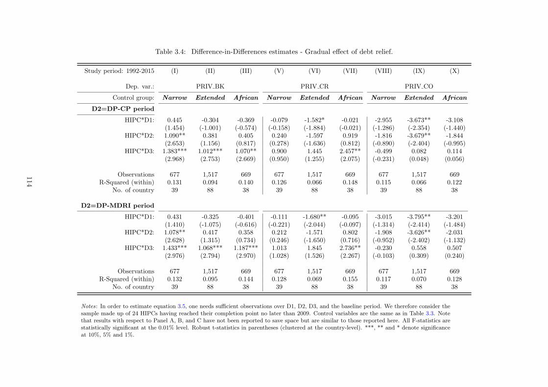
Table 3.4: Difference-in-Differences estimates - Gradual effect of debt relief.

Study period: 1992-2015 (I) (II) (III) (V) (VI) (VII) (VIII) (IX) (X)

Dep. var.: PRIV BK PRIV CR PRIV CO

Control group: Narrow Extended African Narrow Extended African Narrow Extended African

D2=DP-CP period

HIPC*D1: 0.445 -0.304 -0.369 -0.079 -1.582* -0.021 -2.955 -3.673** -3.108(1.454) (-1.001) (-0.574) (-0.158) (-1.884) (-0.021) (-1.286) (-2.354) (-1.440)

HIPC*D2: 1.090** 0.381 0.405 0.240 -1.597 0.919 -1.816 -3.679** -1.844(2.653) (1.156) (0.817) (0.278) (-1.636) (0.812) (-0.890) (-2.404) (-0.995)

HIPC*D3: 1.383*** 1.012*** 1.070** 0.900 1.445 2.457** -0.499 0.082 0.114(2.968) (2.753) (2.669) (0.950) (1.255) (2.075) (-0.231) (0.048) (0.056)

Observations 677 1,517 669 677 1,517 669 677 1,517 669R-Squared (within) 0.131 0.094 0.140 0.126 0.066 0.148 0.115 0.066 0.122

No. of country 39 88 38 39 88 38 39 88 38

D2=DP-MDRI period

HIPC*D1: 0.431 -0.325 -0.401 -0.111 -1.680** -0.095 -3.015 -3.795** -3.201(1.410) (-1.075) (-0.616) (-0.221) (-2.044) (-0.097) (-1.314) (-2.414) (-1.484)

HIPC*D2: 1.078** 0.417 0.358 0.212 -1.571 0.802 -1.908 -3.626** -2.031(2.628) (1.315) (0.734) (0.246) (-1.650) (0.716) (-0.952) (-2.402) (-1.132)

HIPC*D3: 1.433*** 1.068*** 1.187*** 1.013 1.845 2.736** -0.230 0.558 0.507(2.976) (2.794) (2.970) (1.028) (1.526) (2.267) (-0.103) (0.309) (0.240)

Observations 677 1,517 669 677 1,517 669 677 1,517 669R-Squared (within) 0.132 0.095 0.144 0.128 0.069 0.155 0.117 0.070 0.128

No. of country 39 88 38 39 88 38 39 88 38

Notes: In order to estimate equation 3.5, one needs sufficient observations over D1, D2, D3, and the baseline period. We therefore consider thesample made up of 24 HIPCs having reached their completion point no later than 2009. Control variables are the same as in Table 3.3. Notethat results with respect to Panel A, B, and C have not been reported to save space but are similar to those reported here. All F-statistics arestatistically significant at the 0.01% level. Robust t-statistics in parentheses (clustered at the country-level). ***, ** and * denote significanceat 10%, 5% and 1%.

114

3.6.2 Financial environment in high-income countries

Another explanation for such private capital inflows could also be found in the recent

financial turmoils experienced by advanced economies. As regards the recent developments and

especially the two financial crises that severely hit high-income countries (HICs) in 2008 and

2012, one might legitimately think that precautionary behaviors and low returns in high-income

countries have motivated private investors to seek for financial investment with higher returns

and thus to turn toward HIPCs. Such “push factors” were so far captured by time-fixed effects,

included in every regression. However, in this section, we try to go further by identifying whether

HIPCs which, according to our findings have accessed financial markets starting from 2005 on

(the MDRI launching date), have contracted debts to private creditors mostly during financial

busts in advanced economies. To do so, we collect annualized data on the VIX index and the

LIBOR rate (3 months) for our entire period 13 and look at the evolution of those indicators

after 2005. Figure 3.6 below shows that both the VIX and the LIBOR have experienced an

ascending phase prior to the global financial crisis and the sovereign debt issues of European

countries before this trend reversed in 2010 for the VIX and 2007 for the LIBOR. We believe

these indicators can be used as a proxy for the relative attractiveness of low-income countries,

since low levels of VIX and LIBOR denote low market returns in advanced economies (financial

volatility —as regards VIX index— being often associated with bubbles and inflated market re-

turns, which can also be feared by private investors when they feel the bubble is about to deflate).

Figure 3.6: Financial volatility and market returns in high-income countries.

(a) VIX (Financial volatility index) (b) LIBOR rate (3 months)

Notes: Both graphs show the raw evolution (dotted line) of the financial index as well as its smoothed evolution(solid line) derived from weighted local polynomial estimates which have been calculated with the kernel function.Asc.P denotes the ascending phase of the index while Desc.P represents its descending one.

In order to identify the role played by the development of financial markets in high-income

economies (HICs), we interact our variable capturing years in the post-interim period with a

dummy variable capturing years in the descending period as regards these financial indicators,

and alternately a dummy variable identifying years in the ascending period (the CYCLE variable).

13Data have been retrieved from the FRED Economic Data website.

115

This allows us to observe whether HIPCs’ borrowing to private creditors occurred mostly during

the expansion or contraction of financial markets. Results are exposed in Table 3.5. One can

observe that HIPCs borrow from private creditors mostly when both the VIX and LIBOR follow

a downward trend. Indeed, after 2005, many HIPCs of our sample have benefited from both

the HIPC initiative and the MDRI, getting back a substantial borrowing capacity. Yet the

few years following the MDRI where characterized by increasing returns and financial volatility

in advanced economies which did not lead private investors to search for higher returns and

immediately lend to developing countries, and HIPCs in particular. However, when situation

started to depreciate in high-income countries, fall in financial returns have probably motivated

private investors to seek higher returns in developing countries and consider HIPCs as a priority

destination given their renewed debt sustainability.

Moreover, it seems that the decision of private creditors to lend to HIPCs has not been driven

by particular economic or institutional developments in those countries. Indeed, interacting the

post-interim period dummy with indicators such as economic growth, per capita GDP, natural

resource rents, institutional quality, and even the average haircuts on prior defaults to private

creditors (using data from Cruces and Trebesch (2013)) does not lead to observe heterogeneity

in market access among HIPCs (see Table 3.C10 in the Appendix C, p.139). We however notice

that private creditors tend to head toward more stable governments with a significant longevity

in power. Note also that we do not find any negative effect derived from the size of prior haircuts

on sovereign debt owed to private creditors, which emphasizes the absence of lenders’ recall and,

to a certain extent, the ”this time is different” syndrome as defined in Reinhart and Rogoff (2009).

116

Table 3.5: Did financial environment in HICs trigger private capital flows to HIPCs?

(I) (II) (III) (IV) (V) (VI) (VII) (VIII) (IX) (X) (XI) (XII)

Debt relief stage: Interim Period [with at least +6 years after]

VIX LIBOR 3 months

CYCLE Ascending Phase Descending Phase Ascending Phase Descending Phase

Dep. var.: PRIV BK PRIV CR PRIV CO PRIV BK PRIV CR PRIV CO PRIV BK PRIV CR PRIV CO PRIV BK PRIV CR PRIV CO

Narrow CGPost-IP 1.163*** 1.527** 2.491** 0.687*** 0.428 0.890 1.020*** 1.256* 2.061* 0.725*** 0.516 1.004

(3.158) (2.149) (2.185) (2.772) (0.661) (0.922) (3.129) (1.758) (1.898) (3.016) (0.801) (1.046)CYCLE -0.217 -0.733 -1.038 -1.667*** -4.058*** -5.853** -1.155*** -2.497*** -3.100*** -1.541*** -3.746*** -4.609**

(-0.608) (-0.973) (-0.822) (-3.699) (-3.383) (-2.608) (-2.747) (-3.204) (-3.023) (-3.983) (-3.889) (-2.617)Post-IP*CYCLE -0.478 -1.100** -1.595* 0.752* 1.735** 2.535** -0.204 -0.786* -0.936 0.333 0.771 1.146

(-1.507) (-2.452) (-2.017) (1.812) (2.621) (2.073) (-1.007) (-1.706) (-1.253) (1.347) (1.376) (1.400)Observations 593 593 593 593 593 593 593 593 593 593 593 593

Extended CGPost-IP 1.467*** 3.145*** 3.491*** 0.866*** 1.704** 1.725* 1.304*** 3.200*** 3.482*** 0.874*** 0.446 0.370

(3.866) (2.847) (2.830) (3.537) (2.020) (1.874) (4.043) (2.993) (2.982) (2.994) (0.555) (0.411)CYCLE 0.143 -1.219 -0.852 -1.991*** -6.410*** -6.592*** 0.930** 2.866* 3.110* -0.674** -3.835*** -3.376**

(0.556) (-1.401) (-0.867) (-3.821) (-2.970) (-2.965) (2.251) (1.697) (1.785) (-2.464) (-2.881) (-2.457)Post-IP*CYCLE -0.571** -0.768 -1.029 0.858** 2.570*** 3.074** -0.372 -2.361*** -2.609*** 0.454* 2.913*** 3.302***

(-2.085) (-1.415) (-1.371) (2.307) (2.931) (2.604) (-1.498) (-3.559) (-3.076) (1.749) (2.968) (2.916)Observations 1,433 1,433 1,433 1,433 1,433 1,433 1,433 1,433 1,433 1,433 1,433 1,433

African CGPost-IP 1.743** 2.986*** 3.159*** 0.988** 1.680** 1.245 1.599*** 2.899*** 2.823** 0.957* 1.258* 1.023

(2.686) (3.335) (2.808) (2.301) (2.268) (1.150) (2.865) (3.443) (2.477) (1.997) (1.698) (1.075)CYCLE -0.907 -1.857* -2.110** -1.258 -2.628* -4.131** 0.421 0.311 0.189 -1.068* -2.699** -2.472

(-1.514) (-1.775) (-2.078) (-1.525) (-1.922) (-2.095) (1.075) (0.422) (0.322) (-1.783) (-2.362) (-1.495)Post-IP*CYCLE -0.667* -0.928* -1.602 1.221** 2.311*** 3.173** -0.596** -1.490*** -1.494* 0.686** 1.761*** 1.963**

(-1.742) (-1.718) (-1.675) (2.428) (3.216) (2.644) (-2.055) (-3.308) (-1.829) (2.253) (3.098) (2.135)Observations 585 585 585 585 585 585 585 585 585 585 585 585

Notes: Study period runs from 1992 to 2015. Columns (I) to (VI) expose effect of debt relief conditional on the VIX index’s financial cycle (ascending vs. descending phase) while Columns(VII) to (XII) do the same with respect to the LIBOR (3 months) rate. We study changes in disbursements and commitments to private creditors (banks and others) around the interim period.Post-IP is the abbreviation for Post-Interim Period. Note that we control for the same set of explanatory variables used so far. F-stat are not reported (as well as intercepts) in order to savespace but are all significant at the 1% level. Robust t-statistics in parentheses (with standard-errors clustered at the country-level). ***, ** and * denote significance at 10%, 5% and 1%.

117

3.6.3 Flows substitutability

Lastly, one could ultimately wonder whether the increasing resort to external private financing

translates a gradual withdrawal of official creditors in HIPCs. Indeed, given the large amounts

of debt canceled through the HIPC initiative for bilateral lenders, and via the MDRI for the

multilateral donors, official creditors could redirect financing flows towards LICs which did

not benefit from these programs, especially in a context of public finance crisis for most of

the traditional bilateral donors. Debt relief would be thus not additional and HIPCs, which

still lack of sufficient domestic financial resources and need external financing to achieve their

development, would thus have no other choice than seeking for new financing sources such as

private creditors, now reachable given their renewed debt sustainability.

We test this hypothesis by running equation 3.3 but considering as dependent variables gross

financing flows from official donors. Using data from the OECD-DAC, we focus on the effect

of debt relief on changes in grants, gross loans, and gross aid transfers. Following Roodman

(2006), we correct our dependent variables for debt relief flows. We thus remove debt forgiveness

grants from official grants, and rescheduled debt from ODA loans. The gross aid transfers

(GAT) as defined in Roodman (2006) therefore sum corrected measures of grants and ODA

loans. All these variables are expressed in percentage of GDP. In addition, the OECD-DAC

database provides data by type of donors, which conversely to the financing conditions, allows

us to differentiate between bilateral and multilateral creditors in their response to debt relief.

Table 3.A4 in the Appendix A (p.125) provides descriptive statistics for these variables. Note

that we add the same controls as for the financing conditions and test the specification to the

inclusion of different explanatory variables. Table 3.6 below exposes the DID effect of debt relief

on changes in official financing flows. One can notice that in addition of tightening their lending

conditions, official creditors seem to reduce aid flows towards HIPCs (with respect to the various

control groups) by around 4 percentage points of GDP.14 Looking at Table 3.7, it seems that

the fall in official flows materializes by less loans from both multilateral and bilateral donors.

We also observe a diminution in bilateral grants after the decision point and the interim period

which is however not shared by multilateral donors. Results are robust to the set of explanatory

variables as exposed in Table 3.C8 and 3.C9 in the Appendix C (pp.137-138). Note that most of

the explanatory variables are associated with their expected sign when statistically significant.

Conversely to Powell and Bird (2010), these findings suggest that debt relief under these

initiatives has not been additive for HIPCs. This could partly explain the fact that some HIPCs

turned to private creditors and thus tried to access international financial markets at the time

where investors were searching for high-return investment. Therefore, one might think that

borrowing to private creditors has not only been determined by private lenders, but also by

HIPCs themselves in search for necessary financing.

14Note that we ran the same estimates with other official flows (OOF) as dependent variable but did not findany significant effect. Specification using dependent variables expressed in percentage of exports have been alsoused and expose a diminution in gross aid transfers by around 20% of the exports (for bilateral aid transers).Results available upon request to the authors.

118

Table 3.6: Debt relief additionality and changes in traditional official flows.

Study period: 1992-2015 (I) (II) (III) (IV) (V) (VI)

Official donors

Debt relief stage: Decision Point [+8 years after] Interim Period [+6 years after]

Dep. var: Grants Loans GAT Grants Loans GAT

Narrow CGPost-Debt relief stage -2.677*** -2.211*** -4.888*** -2.762*** -2.647*** -5.408***

(-3.633) (-3.422) (-4.712) (-4.189) (-3.567) (-6.140)

Observations 816 816 816 692 692 692R-squared (within) 0.447 0.408 0.492 0.459 0.437 0.521

No. of country 44 44 44 39 39 39

Extended CGPost-Debt relief stage -1.628** -2.261*** -3.890*** -1.416*** -2.566*** -3.982***

(-2.106) (-3.593) (-3.287) (-2.977) (-4.463) (-5.427)

Observations 1,775 1,775 1,775 1,651 1,651 1,651R-squared (within) 0.350 0.275 0.378 0.348 0.309 0.408

No. of country 88 88 88 83 83 83

African CGPost-Debt relief stage -2.098*** -2.694*** -4.793*** -2.240*** -3.325*** -5.566***

(-3.075) (-4.328) (-4.678) (-3.374) (-4.826) (-6.261)

Observations 805 805 805 681 681 681R-squared (wihtin) 0.442 0.382 0.478 0.442 0.425 0.510

No. of country 43 43 43 38 38 38

Notes: Columns (I) to (III) exposes results for a sample of 28 HIPCs that have reached their decision pointno later than 2007. Columns (IV) to (VI) exposes results for a restricted sample of 24 HIPCs that havereached their completion point no later than 2009. The set of control variables is the same for all columnsand includes GDP PC, POP, GDP GROWTH, GFCF, CAB, INF, TOT RESV, DURABLE, andCIVIL L. F-stat are not reported (as well as intercepts) in order to save space but are all significant at the1% level. Robust t-statistics in parentheses (with standard-errors clustered at the country-level). ***, ** and *denote significance at 10%, 5% and 1%.

119

Table 3.7: Debt relief additionality - bilateral vs. multilateral donors.

Study period: 1992-2015 (I) (II) (III) (IV) (V) (VI) (VII) (VIII) (IX) (X) (XI) (XII)

Debt relief stage: Decision Point [with at least +8 years after] Interim Period [with at least +6 years after]

Donors: Bilateral donors Multi donors Bilateral donors Multi donors

Dep. var.: Grants Loans GAT Grants Loans GAT Grants Loans GAT Grants Loans GAT

Narrow CGPost-Debt relief stage -2.343*** -0.464*** -2.807*** -0.335 -1.749*** -2.084*** -2.368*** -0.343* -2.710*** -0.395 -2.310*** -2.705***

(-3.488) (-2.904) (-3.822) (-1.140) (-3.119) (-3.435) (-4.143) (-1.818) (-4.739) (-1.306) (-3.750) (-3.978)

Observations 816 816 816 816 816 816 692 692 692 692 692 692R-squared 0.467 0.203 0.471 0.253 0.377 0.322 0.478 0.309 0.526 0.273 0.379 0.340

No. of country 44 44 44 44 44 44 39 39 39 39 39 39

Extended CGPost-Debt relief stage -1.813*** -0.608*** -2.420*** 0.185 -1.691*** -10.236 -1.681*** -0.402*** -2.083*** 0.266 -2.221*** -1.934***

(-2.689) (-2.909) (-2.941) (0.727) (-3.445) (-0.308) (-4.210) (-2.675) (-4.933) (1.392) (-4.428) (-3.605)

Observations 1,775 1,775 1,775 1,775 1,631 1,631 1,651 1,651 1,651 1,651 1,507 1,507R-squared 0.359 0.133 0.367 0.188 0.258 0.240 0.364 0.161 0.404 0.195 0.295 0.261

No. of country 88 88 88 88 81 81 83 83 83 83 76 76

African CGPost-Debt relief stage -1.988*** -0.686*** -2.675*** -0.111 -2.008*** -2.119*** -2.125*** -0.648*** -2.773*** -0.116 -2.678*** -2.794***

(-3.228) (-3.799) (-3.693) (-0.400) (-3.738) (-3.459) (-3.856) (-3.958) (-4.986) (-0.438) (-4.427) (-4.012)

Observations 805 805 805 805 805 805 681 681 681 681 681 681R-squared 0.459 0.195 0.469 0.257 0.335 0.300 0.459 0.307 0.520 0.278 0.360 0.326

No. of country 43 43 43 43 43 43 38 38 38 38 38 38

Notes: Columns (I) to (III) and (VII) to (IX) exposes effect of debt relief on changes in financing flows from bilateral donors (DAC and non-DAC). Other columns report theeffect of debt relief on changes in multilateral financing flows. We observe these debt relief effects both around the decision point (Columns (I) to (VI)) and the interim period(Columns (VII) to (XII)) with their respective HIPCs sample. The set of control variables is the same for all columns and includes GDP PC, POP, GDP GROWTH, GFCF,CAB, INF, TOT RESV, DURABLE, and CIVIL L. F-stat are not reported (as well as intercepts) in order to save space but are all significant at the 1% level. Robustt-statistics in parentheses (with standard-errors clustered at the country-level). ***, ** and * denote significance at 10%, 5% and 1%.

120

3.7 Conclusion

Results of this study show that debt relief initiatives have probably affected HIPCs’ external

public financing. They suggest that having benefited from the Enhanced HIPC initiative leads

official lenders to tighten their lending conditions by shortening both grace and maturity periods

on new loans (with respect to non-HIPCs). Such adjustments seems to reduce in fine the

grant element on new official external public debt for HIPCs. Moreover, given the rigidity of

multilateral donors’ financing policies, we suspect this tightening of lending conditions on new

loans to be mostly driven by bilateral creditors seeking higher returns on their investments,

especially in a context of budgetary discipline. Furthermore, additional results support that

both bilateral and multilateral creditors reduced official financing flows toward HIPCs after

having granted debt relief (and as compared with flows provided to non-HIPCs); the reduction

in bilateral flows being more pronounced than for multilateral donors.

We think this probably led HIPCs to search for alternative sources of financing. Our study

tends to show that HIPCs might have found such opportunities by accessing (again, for some of

them) the international financial markets after having been granted full and irrevocable debt

relief. As shown by results in Section 6, HIPCs seem to contract more debt from private creditors

once they have benefited from ultimate debt cancellations under the MDRI (i.e. once all their

remaining multilateral debt stock has been canceled) and when financial markets in high-income

countries endure bearish dynamics.

In sum, it appears that the positive impact of debt cancellations on debt sustainability leads

official creditors to propose financing to HIPCs on terms that are closer to “real market” conditions.

This behavior might even be reinforced by HIPCs’ borrowing to private creditors which illustrate

the capacity of these countries to contract loans at market conditions. These initiatives have

thus driven up the financing opportunities by making borrowing on the international financial

markets accessible for countries historically excluded from them. In a way, one might think that

debt relief initiatives have helped relieve the “double original sin” that weighed on HIPCs.

Nevertheless, a close eye should be kept on this new borrowing dynamics in order to prevent

future unsustainable debt levels. As detailed above, debt to private creditors is often associated

with high interest rates, which can easily lead to repayment issues. In October 2015, the

IMF Regional Economic Outlook reported that some HIPCs such as Zambia, Senegal, Ghana,

Gambia, and Malawi were expected to reach, in 2016, debt-to-GDP ratios twice higher than

the level recorded right after the MDRI. Even more worrying is the fact that some HIPCs such

as Mozambique are suffering from the fall in international commodity prices and are already

experiencing repayment difficulties. Stiglitz may have got it right, again.

121

Complementary results

Appendix A. Control variables: descriptive statistics and expected effects.

Table 3.A1: Descriptive Statistics - Whole sample (112 DCs) [1992-2015]

Variables Source Unit Mean Std. Dev. Obs. % missings

Dependent variables

AGP IDS 2016 years 6.14 3.23 2677 1.76AM IDS 2016 years 23.21 11.93 2678 1.72AGE IDS 2016 in % 54.28 19.48 2415 11.37AGE MO authors’ comput. in % 71.81 21.54 2411 11.52AGE MT authors’ comput. in % 64.20 26.25 2658 2.45PRIV BANK IDS 2016 % of exports 0.77 2.65 2725 0.00PRIV CRED IDS 2016 % of exports 2.77 7.94 2725 0.00PRIV CO IDS 2016 % of exports 2.88 8.38 2725 0.00

Explanatory variables

GDP PC WDI 2016 constant USD, log 7.43 1.02 2644 2.97POP WDI 2016 inhabitants, log 15.85 1.90 2708 0.62GDP GROWTH WDI 2016 % change 4.13 6.19 2652 2.67GFCF WDI 2016 % of GDP 23.52 9.84 2446 10.23RES RENT WDI 2016 % of GDP 10.76 13.56 2427 10.93CAB WDI 2016 % of GDP -11.76 14.98 2626 3.63TOT RES WDI 2016 months of imp. 4.44 3.77 2235 17.98INF WDI 2016 % change 48.12 716.88 2464 9.57POLIT IV Polity IV [-10; 10] 1.99 5.99 2409 11.59CIVIL L Freedom House [1; 7] 4.06 1.51 2697 1.02DURABLE Polity IV years 14.72 16.66 2457 9.83KOF Dreher (2006) index 44.09 12.01 2435 10.64CPIA CPIA index 3.23 0.60 2146 21.24ECO FREE Heritage Foundation index 55.45 8.33 2025 25.68EXP DIVERS IMF index 3.68 1.04 2049 24.80

Notes: This table exposes descriptive statistics for the whole sample that includes both HIPCs and control group countries.The entire sample consists in an unbalanced sample of 112 developing countries observed between 1992 and 2015.

122

Table 3.A2: Explanatory variables: expected effects on official financing conditions (and related literature).

Variables Definition expect. sign Studies

GDP PC GDP per capita (constant USD, log) -Knight and Santaella (1997), Alesina and Dollar (2000),Bird and Rowlands (2001), Neumayer (2003),Berthelemy and Tichit (2004), Berthelemy (2006), Dollar and Levin (2006), Harrigan et al. (2006),Claessens et al. (2009), Fleck and Kilby (2010), Hoeffler and Outram (2011)

POP Total population (log) -Snyder (1993), Alesina and Dollar (2000), Berthelemy and Tichit (2004), Berthelemy (2006),Claessens et al. (2009), Fleck and Kilby (2010), Hoeffler and Outram (2011)

GDP G GDP growth (%) -Knight and Santaella (1997), Bird and Rowlands (2001), Berthelemy and Tichit (2004),Harrigan et al. (2006), Dreher et al. (2009b), Hoeffler and Outram (2011)

GFCF Total Investment (% GDP) - Knight and Santaella (1997), Harrigan et al. (2006), Dreher et al. (2009b), Dreher et al. (2009a)

CAB Curr. account net from ext. grants (% GDP) -Knight and Santaella (1997), Bird and Rowlands (2001), Harrigan et al. (2006),Dreher et al. (2009b), Dreher et al. (2009a)

TOT RESV International reserves (months of imports) -Knight and Santaella (1997), Bird and Rowlands (2001), Harrigan et al. (2006),Dreher et al. (2009b), Dreher et al. (2009a)

POLIT IV Polity IV - autocracy/democracy +/-Alesina and Dollar (2000), Alesina and Weder (2002), Neumayer (2003), Berthelemy and Tichit (2004),Berthelemy (2006), Dollar and Levin (2006), Harrigan et al. (2006) ,Fleck and Kilby (2010), Hoeffler and Outram (2011), Dreher et al. (2009b)

DURABLE Durability of the government + Knight and Santaella (1997), Bird and Rowlands (2001), Harrigan et al. (2006), Fleck and Kilby (2010),Hoeffler and Outram (2011), Dreher et al. (2009b), Dreher et al. (2009a)

CIVIL L Civil Liberties/Freedom + Alesina and Dollar (2000), Bird and Rowlands (2001), Neumayer (2003), Hoeffler and Outram (2011)

INF Inflation rate -/+ Knight and Santaella (1997), Dreher et al. (2009b), Dreher et al. (2009a)

CPIA Institutional quality -/+ Claessens et al. (2009), Marchesi and Missale (2013)

UN VOTE Vote alignment at the UN gen. assembly + Alesina and Dollar (2000), Hoeffler and Outram (2011), Dreher et al. (2009b), Dreher et al. (2009a)

Notes: Studies in bold font focus on the determinants of multilateral aid or assistance to developing countries while these in normal font aim at identifying the drivers of bilateral aid allocation. Studies in bold anditalic font investigate both multilateral and bilateral financing determinants.

123

Table 3.A3: Explanatory variables: expected effects on financing to private creditors (and related literature).

Variables Definition expect. sign Studies

GDP PC GDP per capita (constant USD, log) +Cantor and Packer (1996), Eichengreen et al. (2002), Afonso (2003), Afonso et al. (2007),Borensztein and Panizza (2009), Gelos et al. (2011), Richmond and Dias (2008), Benczur and Ilut (2015)

GDP G GDP growth (%) +Edwards (1984), Cantor and Packer (1996), Afonso (2003), Borensztein and Panizza (2009),Gelos et al. (2011), Richmond and Dias (2008), Benczur and Ilut (2015)

CAB Current account balance net from ext. grants -/+Edwards (1984), Cantor and Packer (1996),Ferrucci (2003), Afonso et al. (2007),Borensztein and Panizza (2009), Baldacci et al. (2008), Cruces and Trebesch (2013)

TOT RESV International reserves (in months of imports) +Edwards (1984), Afonso et al. (2007), Baldacci et al. (2008), Gelos et al. (2011),Hilscher and Nosbusch (2010),Cruces and Trebesch (2013), Benczur and Ilut (2015)

INF Inflation rate -Cantor and Packer (1996), Borensztein and Panizza (2009), Baldacci et al. (2008),Eichengreen et al. (2002), Afonso (2003), Afonso et al. (2007), Baldacci et al. (2008)

DURABLE/Political/Economic risk -

Borensztein and Panizza (2009), Gelos et al. (2011), Cruces and Trebesch (2013)ECO FREE Cruces and Trebesch (2013), Trebesch and Zabel (2017)

CPIA Institutional quality + Eichengreen et al. (2002), Afonso et al. (2007),Gelos et al. (2011)

KOFE Globalization/openness index +Edwards (1984), Borensztein and Panizza (2009), Gelos et al. (2011),Eichengreen et al. (2002), Ferrucci (2003)

HAIR CUT Size of the haircut on prior restructuring - Cruces and Trebesch (2013); Trebesch and Zabel (2017)

124

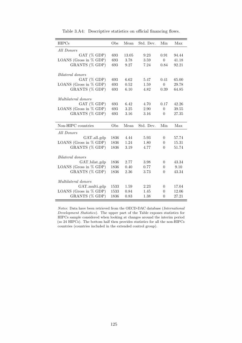
Table 3.A4: Descriptive statistics on official financing flows.

HIPCs Obs Mean Std. Dev. Min Max

All DonorsGAT (% GDP) 693 13.05 9.23 0.91 94.44

LOANS (Gross in % GDP) 693 3.78 3.59 0 41.18GRANTS (% GDP) 693 9.27 7.24 0.84 92.21

Bilateral donorsGAT (% GDP) 693 6.62 5.47 0.41 65.00

LOANS (Gross in % GDP) 693 0.52 1.59 0 29.78GRANTS (% GDP) 693 6.10 4.82 0.39 64.85

Multilateral donorsGAT (% GDP) 693 6.42 4.70 0.17 42.26

LOANS (Gross in % GDP) 693 3.25 2.90 0 39.55GRANTS (% GDP) 693 3.16 3.16 0 27.35

Non-HIPC countries Obs Mean Std. Dev. Min Max

All DonorsGAT all gdp 1836 4.44 5.93 0 57.74

LOANS (Gross in % GDP) 1836 1.24 1.80 0 15.31GRANTS (% GDP) 1836 3.19 4.77 0 51.74

Bilateral donorsGAT bilat gdp 1836 2.77 3.98 0 43.34

LOANS (Gross in % GDP) 1836 0.40 0.77 0 9.10GRANTS (% GDP) 1836 2.36 3.73 0 43.34

Multilateral donorsGAT multi gdp 1533 1.59 2.23 0 17.04

LOANS (Gross in % GDP) 1533 0.84 1.45 0 12.06GRANTS (% GDP) 1836 0.83 1.38 0 27.21

Notes: Data have been retrieved from the OECD-DAC database (InternationalDevelopment Statistics). The upper part of the Table exposes statistics forHIPCs sample considered when looking at changes around the interim period(so 24 HIPCs). The bottom half then provides statistics for all the non-HIPCscountries (countries included in the extended control group).

125

Appendix B. Control groups: composition and suitability.

Table 3.B1: ”Extended” control group countries.

Albania Dominica Lebanon Sri LankaAlgeria Dominican Republic Lesotho St. LuciaAngola Ecuador Malaysia St. VincentArgentina Egypt Maldives SudanArmenia El Salvador Mauritius SwazilandAzerbaijan Eritrea Moldova SyriaBangladesh Fiji Mongolia TajikistanBelarus Georgia Morocco ThailandBelize Grenada Myanmar TongaBhutan Guatemala Nepal TunisiaBosnia and Herzegovina India Nigeria TurkeyBotswana Indonesia Pakistan TurkmenistanBrazil Iran. Islamic Rep. Panama UkraineCambodia Jamaica Papua New Guinea UzbekistanCape Verde Jordan Paraguay VanuatuChina Kazakhstan Peru VenezuelaColombia Kenya Philippines VietnamCosta Rica Kyrgyz Republic Serbia YemenDjibouti Lao PDR South Africa Zimbabwe

Narrow control group countriesAfrican control group countries

126

Table 3.B2: Pre-Debt relief period: Descriptive statistics on covariates.

(I) (II) (III) (IV)

Pre-Decision Point Mean

Variable / Group: HIPC DP Narrow CG Extended CG African CG

Debt (% of exports) 615.33 350.11 162.75 218.79LIC Status 0.93 0.94 0.31 0.39

GDP PC (in log) 6.34 6.60 7.67 7.52POP (inhabitants, log) 15.85 17.08 15.78 15.90

GDP GROWTH (% change) 3.63 4.56 3.83 3.83GFCF (% of GDP) 17.65 21.83 24.15 24.89

RES RENT (% of GDP) 13.75 10.51 7.58 10.26CAB (% of GDP) -18.72 -11.07 -8.21 -8.37

TOT RESV (% of GDP) 2.84 2.88 3.81 4.46INF (% change) 21.45 23.52 56.18 105.30

POLIT IV 1.25 -0.99 1.45 -1.25CIVIL L 4.31 5.09 4.21 4.62

DURABLE 6.09 13.87 15.77 12.46KOF 34.62 33.58 42.86 41.84CPIA 3.03 3.09 3.23 3.06

ECO FREE 52.95 48.53 54.88 53.78EXP DIVERS 4.35 3.54 3.40 3.65

Pre-Decision Point - Difference in Mean

Variable / Diff: (I) (I) - (II) (I)-(III) (I-IV)

Debt (% of exports) - 265.21*** 452.57*** 396.53***LIC Status - -0.01 0.61*** 0.54***

GDP PC (in log) - -0.25*** -1.32*** -1.17***POP (inhabitants, log) - -1.23*** 0.07 -0.04

GDP GROWTH (% change) - -0.93* -0.20 -0.20GFCF (% of GDP) - -4.18*** -6.49*** -7.24***

RES RENT (% of GDP) - 3.24*** 6.16*** 3.49***CAB (% of GDP) - -7.65*** -10.50*** -10.35***

TOT RESV (% of GDP) - -0.04 -0.96*** -1.61***INF (% change) - -2.06 -34.73*** -83.84***

POLIT IV - 2.10*** -0.31 2.36***CIVIL L - -0.77*** 0.10 -0.30***

DURABLE - -7.78*** -9.68*** -6.37***KOF - 1.03 -8.24 -7.22***CPIA - -0.05 -0.20*** -0.03

ECO FREE - 4.41*** -1.92*** -0.82EXP DIVERS - 0.81*** 0.94*** 0.70***

Notes: Mean values have been computed over the 6 years preceding the decision point of each HIPC.For control groups, we have calculated the weighted average across control group countries and overthe 6 years before the decision point of their associated HIPCs’ cohort (see explanations in Figure 3.2,p.103). ***, ** and * denote significance at 10%, 5% and 1%.

127

Table 3.B3: Pre-Debt relief period: Descriptive statistics on outcome variables.

(I) (II) (III) (IV) (V)

Pre Decision-Point Mean

Variable / Group: HIPC DP HIPC IP Narrow CG Extended CG African CG

AGP (in years) 8.11 8.42 7.33 5.72 4.79AMP (in years) 31.58 32.71 26.75 20.99 18.73

AGE (in %) 69.23 69.45 56.97 42.25 41.56AGE MO (in %) 87.05 86.86 69.33 58.86 61.83AGE MT (in %) 85.29 84.62 68.57 51.18 53.16

PRIV BK 0.14 0.17 0.71 1.30 1.68PRIV CR 0.67 0.77 1.54 4.48 3.62PRIV CO 0.83 0.96 1.51 4.59 3.39

Pre-Decision Point - Difference in Mean

Variable / Diff: (I) (II) (I) - (III) (I)-(IV) (I-V)

AGP (in years) - - 0.78*** 2.39*** 3.31***AMP (in years) - - 4.83*** 10.59*** 12.85***

AGE (in %) - - 12.26*** 26.97*** 27.67***AGE MO (in %) - - 17.71*** 28.19*** 25.22***AGE MT (in %) - - 16.71*** 34.10*** 32.12***

PRIV BK - - -0.57*** -1.15*** -1.54***PRIV CR - - 0.86*** -3.81*** -2.95***PRIV CO - - -0.65* -3.75*** 2.56***

Notes: Mean values have been computed over the 6 years preceding the decision point of each HIPCs.For control groups, we have calculated the average across control group countries and over the 6years before the decision point of their associated HIPCs’ cohort (see explanations in Figure 3.2,p.103). ***, ** and * denote significance at 10%, 5% and 1%.

128

Table 3.B4: Event-Study - Test for parallel trends prior debt relief.

(I) (II) (III) (IV) (V) (VI) (VII) (VIII)

Period Placebo test [-6;-4] vs [-3; -1]

Dep. var. AGP AMP AGE AGE MO AGE MT PRIV BK PRIV CR PRIV CO

Narrow Control GroupPost Placebo-Period 0.125 1.660 -1.587 1.012 3.198** -0.037 -0.352* -1.218

(0.419) (1.365) (-0.980) (1.002) (2.715) (-0.510) (-1.985) (-1.621)

Extended Control GroupPost Placebo-Period 0.413 1.456 -1.274 1.169 2.074* -0.311*** -1.563*** -2.001***

(1.442) (1.208) (-0.766) (1.118) (1.823) (-3.965) (-5.228) (-2.986)

African Control GroupPost Placebo-Period 0.430 2.158* -4.568*** -2.345** -1.420 -0.503*** 0.377** -0.856

(1.594) (1.718) (-2.849) (-2.396) (-1.197) (-5.208) (2.409) (-1.149)

Number of HIPCs 29 29 29 29 29 29 29 29Country Fixed Effects Yes Yes Yes Yes Yes Yes Yes Yes

Observations 174 174 160 160 174 174 174 174

Notes: Robust t-statistics (with standard-errors clustered at the country-level) in parentheses. ***, ** and * denotesignificance at 10%, 5% and 1%.

129

Appendix C. Robustness checks: covariates, control groups, and sample dependence.

Table 3.C1: Alternative selection criteria, alternative control groups.

Panel A

Debt-to-dom.rev. sup. 250 % andLIC average status at least (3/5)

Bangladesh Bhutan CambodiaGeorgia Indonesia Kyrgyz RepublicLao PDR Nepal PakistanSudan Tajikistan VietnamYemen Zimbabwe

Panel B

Debt-to-Exports Ratio sup. 170 % andLIC average status at least (0/5)

Algeria Argentina BangladeshBhutan Cambodia Cabo VerdeDominica Ecuador EgyptEritrea Georgia GrenadaIndia Jordan Kenya

Kyrgyz Republic Lao PDR LebanonLesotho Morocco NepalNigeria Pakistan PeruSamoa Serbia TongaSudan Syria VietnamYemen Zimbabwe

Panel C

Debt-to-Exports Ratio sup. 0 % andLIC average status at least (5/5)

Armenia Azerbaijan BangladeshBhutan Cambodia EritreaIndia Kenya Kyrgyz Republic

Lao PDR Lesotho MoldovaMongolia Nepal NigeriaPakistan Sudan Tajikistan

Uzbekistan Vietnam YemenZimbabwe

130

Table 3.C2: DID estimates - Sensitivity to the narrow control group.

Study period: 1992-2015 (I) (II) (III) (IV) (V) (VI) (VII) (VIII)

Debt relief stage: Decision Point [with at least +8 years after]

Dep. var.: AGP AMP AGE AGE MO AGE MT PRIV BK PRIV CR PRIV CO

Panel APost-Decision Point -0.769 -3.787* -9.583** -11.630** -4.904 0.723*** 0.501 1.024

(-1.359) (-1.764) (-2.476) (-2.107) (-1.431) (2.867) (0.966) (1.576)

Observations 758 758 734 734 756 699 699 699R-squared (within) 0.165 0.150 0.123 0.326 0.273 0.131 0.140 0.109

No. of country 42 42 42 42 42 40 40 40

Panel BPost-Decision Point -0.816 -4.415** -9.114*** -11.270*** -10.081** 0.890*** 1.909 2.365*

(-1.484) (-2.343) (-2.989) (-3.003) (-2.605) (3.162) (1.588) (1.760)

Observations 950 950 915 915 945 879 879 879R-squared (within) 0.139 0.093 0.133 0.298 0.233 0.118 0.052 0.053

No. of country 51 51 51 51 51 51 51 51

Panel CPost-Decision Point -1.179* -5.840** -8.731** -11.673** -10.011** 0.924*** 1.296** 1.940**

(-1.731) (-2.450) (-2.153) (-2.014) (-2.116) (3.674) (2.189) (2.484)

Observations 893 893 863 863 890 827 827 827R-squared (within) 0.178 0.103 0.108 0.278 0.264 0.119 0.087 0.081

No. of country 48 48 48 48 48 48 48 48

Notes: Table exposes results for a sample of 28 HIPCs that have reached their decision point no later than 2007. The set ofcontrol variables is the same as for Table 3.2. Panel A: Debt/Revenue sup. 250% and LIC Status at least (3/5), 14 controlgroup countries; Panel B: Debt/Exports sup. 170% and LIC status at least (0/5), 32 control group countries; Panel C:Debt/Exports sup. 0% and LIC status at least (5/5), 22 control group countries. F-stat are not reported (as well as intercepts)in order to save space but are all significant at the 1% level. Robust t-statistics in parentheses (with standard-errors clustered atthe country-level). ***, ** and * denote significance at 10%, 5% and 1%.

131

Table 3.C3: DID estimates - Sensitivity to the narrow control group (continued).

Study period: 1992-2015 (I) (II) (III) (IV) (V) (VI) (VII) (VIII)

Debt relief stage: Interim Period [with at least +6 years after]

Dep. var.: AGP AMP AGE AGE MO AGE MT PRIV BK PRIV CR PRIV CO

Panel APost-Interim Period -1.560** -5.468** -14.693*** -17.093*** -7.147 0.873*** 0.807 1.424

(-2.376) (-2.342) (-3.431) (-2.751) (-1.593) (3.050) (1.405) (1.669)

Observations 634 634 622 622 632 548 548 548R-squared (within) 0.197 0.151 0.158 0.363 0.280 0.138 0.144 0.111

No. of country 37 37 37 37 37 36 36 36

Panel BPost-Interim Period -1.319** -6.545*** -13.968*** -15.670*** -13.346*** 1.062*** 3.805* 4.297**

(-2.230) (-3.127) (-3.942) (-4.006) (-3.270) (3.287) (1.896) (2.059)

Observations 826 826 803 803 821 728 728 728R-squared (within) 0.157 0.089 0.167 0.329 0.244 0.129 0.076 0.074

No. of country 46 46 46 46 46 47 47 47

Panel CPost-Interim Period -1.808** -8.489*** -13.115*** -16.905** -13.356** 1.160*** 1.990*** 2.624***

(-2.397) (-3.026) (-2.871) (-2.647) (-2.531) (4.111) (2.737) (2.756)

Observations 769 769 751 751 766 676 676 676R-squared (within) 0.204 0.099 0.122 0.308 0.280 0.138 0.100 0.089

No. of country 43 43 43 43 43 44 44 44

Notes: Table exposes results for a sample of 24 HIPCs that have reached their completion point no later than 2009. The set ofcontrol variables is the same as for Table 3.2. Panel A: Debt/Revenue sup. 250% and LIC Status at least (3/5), 14 controlgroup countries; Panel B: Debt/Exports sup. 170% and LIC status at least (0/5), 32 control group countries; Panel C:Debt/Exports sup. 0% and LIC status at least (5/5), 22 control group countries. F-stat are not reported (as well as intercepts)in order to save space but are all significant at the 1% level. Robust t-statistics in parentheses (with standard-errors clustered atthe country-level). ***, ** and * denote significance at 10%, 5% and 1%.

132

Table 3.C4: Falsification tests.

(I) (II) (III) (IV) (V) (VI) (VII) (VIII)

Effect of having reached: the Decision Point

Dep var.: AGP AMP AGE AGE MO AGE MT PRIV BK PRIV CR PRIV CO

Random draw replication: 500

Coefficient for Post-Decision PointMean -0.006 -0.003 -0.050 -0.283 0.036 -0.014 -0.009 -0.001

Standard deviation 0.402 1.540 2.887 3.439 2.821 0.328 1.375 1.337Percent significant 4.80 4.20 4.20 3.80 4.40 6.60 14.60 8.40

Observations 1,769 1,769 1,668 1,667 1,764 1,584 1,584 1,584No. of country 88 88 88 88 88 92 92 92

Country FE Yes Yes Yes Yes Yes Yes Yes YesTime FE Yes Yes Yes Yes Yes Yes Yes Yes

Effect of having fully completed: the Interim Period

Dep var.: AGP AMP AGE AGE MO AGE MT PRIV BK PRIV CR PRIV CO

Random draw replication: 500

Coefficient for Post-Decision PointMean 0.031 0.094 -0.190 0.297 0.307 0.015 -0.068 -0.089

Standard deviation 0.512 2.098 3.699 4.531 3.543 0.440 1.494 1.636Percent significant 4.33 6.33 5.00 2.67 4.00 9.67 12.00 8.33

Observation 1,645 1,645 1,556 1,556 1,640 1,433 1,433 1,433No. of country 83 83 83 83 83 88 88 88

Country FE Yes Yes Yes Yes Yes Yes Yes YesTime FE Yes Yes Yes Yes Yes Yes Yes Yes

Notes: The upper part of the Table presents the effect of having reached the decision point on our variables representing thefinancing conditions to official creditors and debt inflows from private creditors. The second part of the Table reports the effect ofhaving fully benefited from the interim period on the same dependent variables. We randomly draw samples of treated countries,estimate the effect of having benefited from debt relief under the decision point or the entire interim period, and then replicatethe operation 500 times (or 300 times but not reported here in order to save space). The average statistics (mean and standarderror) on the coefficient of interest are reported below the number of replications. Finally, the raw “Percent significant” reportsthe percentage of estimates where the coefficient of interest is statistically significant at the 10% level (over the 500 replications).All the estimates account for macroeconomic covariates as in the main specifications.

133

Table 3.C5: DID estimates w/r to the extended control group.

Period: 1992-2015* (I) (II) (III) (IV) (V) (VI) (VII) (VIII) (IX) (X) (XI) (XII)

Debt relief stage: Interim Period [with at least +6 years after]

Dep. var.: AGP AMP AGE AGE MO

Post-Interim Period -1.287** -1.319** -0.704 -4.864*** -4.927*** -2.411 -16.784*** -16.760*** -8.743** -13.806*** -13.779*** -7.682(-2.493) (-2.550) (-1.285) (-2.818) (-2.836) (-1.214) (-5.347) (-5.324) (-2.596) (-3.563) (-3.523) (-1.653)

GDP PC -1.229 -1.223 1.370 -2.471 -2.322 5.239 -18.169*** -18.068*** -3.132 -16.748*** -17.081*** -6.811(-1.539) (-1.517) (1.395) (-0.825) (-0.767) (1.172) (-3.798) (-3.805) (-0.489) (-2.810) (-2.916) (-1.019)

POP 1.262 1.116 6.789** 6.824 6.791 23.369** -11.506 -11.286 20.978 -2.574 -2.866 4.903(0.729) (0.652) (2.562) (1.050) (1.075) (2.321) (-0.882) (-0.870) (1.338) (-0.143) (-0.159) (0.219)

GDP G 0.040** 0.040** 0.028 0.132** 0.135** 0.083 0.199* 0.200* 0.132 0.355*** 0.350*** 0.205(2.573) (2.612) (1.175) (2.427) (2.470) (0.928) (1.830) (1.826) (0.797) (3.447) (3.411) (1.287)

GFCF 0.002 0.002 -0.005 0.006 0.007 -0.035 -0.051 -0.049 -0.035 -0.154** -0.158** -0.127(0.175) (0.153) (-0.348) (0.159) (0.172) (-0.655) (-0.644) (-0.628) (-0.351) (-2.232) (-2.284) (-1.289)

CAB 0.004 0.003 0.022 -0.001 -0.005 0.056 -0.113* -0.114* 0.044 -0.238*** -0.231*** -0.139**(0.295) (0.238) (1.650) (-0.039) (-0.137) (1.182) (-1.802) (-1.809) (0.736) (-4.529) (-4.506) (-1.996)

TOT RESV 0.056 0.056 -0.017 0.226* 0.239* 0.073 0.725** 0.739** 0.686** 1.077*** 1.035*** 1.060***(1.464) (1.465) (-0.261) (1.676) (1.756) (0.289) (2.094) (2.121) (2.062) (2.941) (2.766) (2.941)

INF -0.000 -0.000 0.000 -0.000 -0.000 0.001 -0.000 0.000 -0.000 0.008*** 0.008*** 0.005***(-0.301) (-0.447) (1.621) (-0.220) (-0.244) (1.579) (-0.036) (0.018) (-0.279) (2.738) (2.666) (3.323)

DURABLE 0.011 0.012 0.001 0.043 0.042 -0.008 0.147** 0.143** 0.052 0.080 0.088 -0.168(1.167) (1.290) (0.036) (1.314) (1.270) (-0.143) (2.528) (2.540) (0.492) (0.783) (0.877) (-1.074)

CIVIL L -0.230* -0.717* -0.134 0.997(-1.858) (-1.787) (-0.170) (1.137)

POLIT IV 0.060** 0.079 -0.078 0.054(2.341) (0.922) (-0.439) (0.313)

CPIA 0.292 1.269 0.696 1.864(1.032) (1.118) (0.382) (0.711)

UN VOTE 3.027 30.308 14.535 -53.717(0.357) (1.057) (0.257) (-0.927)

Obs 1,645 1,645 947 1,645 1,645 947 1,556 1,556 915 1,555 1,555 914R-Squared (within) 0.079 0.081 0.072 0.060 0.059 0.071 0.227 0.227 0.141 0.243 0.242 0.185

No. of country 83 83 77 83 83 77 83 83 77 83 83 77

Notes: Table exposes changes in dependent variable around the interim period for a sample of 24 HIPCs that have reached their completion point no later than 2009. DIDestimates for each dependent variable are obtained with respect to the extended control group. We do not report results for AGE MT since they are really similar to those forAGE MO. *Note that when including data on UN VOTE, the study period is shortened to 1992-2008, which excludes HIPCs ending the process after 2007 and reduces thepost-interim period for other HIPCs. Robust t-statistics in parentheses (with standard-erros clustered at the country-level). ***, ** and * denote significance at 10%, 5% and 1%.

134

Table 3.C6: DID estimates w/r to the extended control group (continued).

Period: 1992-2015 (I) (II) (III) (IV) (V) (VI) (VII) (VIII) (IX) (X) (XI) (XII)

Debt relief stage: Interim Period [with at least +6 years after]

Dep. var.: PRIV BK PRIV CR PRIV CO

Post-Interim Period 1.250*** 0.889*** 1.043*** 1.095*** 2.854*** 1.717* 1.607 1.981* 3.100*** 1.677* 1.502 2.066*(4.049) (4.167) (2.974) (3.264) (2.798) (1.748) (1.475) (1.971) (2.818) (1.675) (1.271) (1.900)

GDP PC 2.010*** 1.644*** 2.533*** 1.686** 3.228 4.773** 4.862** 1.209 5.405* 4.971** 7.349** 2.878(2.773) (2.988) (2.798) (2.553) (1.019) (2.091) (2.150) (0.758) (1.714) (2.158) (2.177) (1.492)

GDP G -0.018 -0.034** -0.043** -0.022 -0.044 -0.062*** -0.069** -0.025 -0.043 -0.059** -0.074 -0.029(-1.616) (-2.483) (-2.205) (-1.651) (-1.236) (-3.039) (-2.028) (-0.780) (-1.027) (-2.442) (-1.359) (-0.708)

CAB -0.015* -0.016* -0.015 -0.009 -0.055** -0.034 -0.039 -0.021 -0.045* -0.036 -0.042 -0.030(-1.704) (-1.678) (-1.262) (-1.314) (-2.109) (-1.294) (-1.607) (-1.044) (-1.868) (-1.356) (-1.642) (-1.299)

TOT RESV -0.086* -0.014 -0.042 -0.207 0.143 0.052 -0.242 0.142 0.013(-1.947) (-0.275) (-0.968) (-1.073) (0.976) (0.422) (-1.253) (0.932) (0.095)

INF -0.000 -0.000 0.000 -0.000 0.000 -0.000(-1.170) (-1.491) (0.960) (-0.640) (0.813) (-0.737)

DURABLE -0.013 -0.012 -0.008 -0.075** -0.077 -0.063 -0.071* -0.076 -0.062(-1.074) (-0.917) (-0.621) (-2.045) (-1.603) (-1.588) (-1.897) (-1.659) (-1.528)

ECO FREE -0.034 -0.029 -0.037 0.006 0.020 0.118 -0.024 -0.038 0.078(-1.024) (-0.729) (-0.913) (0.060) (0.281) (1.168) (-0.223) (-0.457) (0.702)

CPIA -0.347 1.250 1.151(-0.983) (1.158) (1.067)

KOF 0.033 0.053 0.278*** 0.279*** 0.251** 0.270***(1.027) (1.430) (2.845) (3.028) (2.491) (2.772)

RES RENT 0.001 -0.004 -0.023(0.089) (-0.125) (-0.655)

Obs 1,433 1,952 1,059 1,297 1,433 1,952 1,059 1,297 1,433 1,952 1,059 1,297R-Squared (within) 0.094 0.033 0.074 0.085 0.067 0.049 0.075 0.115 0.062 0.040 0.061 0.092

No. of country 88 97 81 83 88 97 81 83 88 97 81 83

Notes: Table exposes changes in dependent variable around the interim period for a sample of 24 HIPCs that have reached their completion point no later than 2009. DIDestimates for each dependent variable are obtained with respect to the extended control group. Robust t-statistics in parentheses (with standard-erros clustered at thecountry-level). ***, ** and * denote significance at 10%, 5% and 1%.

135

Table 3.C7: DID estimates - Outliers and sample sensitivity.

(I) (II) (III) (IV) (V) (VI) (VII)

Dep. var.: PPG Debt - Disbursements to private banks

with respect to the Narrow Control Group

Debt relief stage: Decision Point [with at least +8 years after]

excluding: Benin Bolivia Burkina Faso Burundi Cameroon CAF Chad

Post-DP 0.811*** 0.804*** 0.824*** 0.832*** 0.807*** 0.865*** 0.831***(3.080) (3.106) (3.065) (3.193) (3.098) (3.162) (3.181)

excluding: Congo Ethiopia Gambia Ghana Guinea Guinea-B Guyana

Post-DP 0.868*** 0.642*** 0.815*** 0.858*** 0.802*** 0.819*** 0.840***(3.263) (2.876) (3.128) (3.131) (3.079) (3.095) (3.115)

excluding: Honduras Madagasc. Malawi Mali Mauritan. Mozamb. Nicaragua

Post-DP 0.819*** 0.803*** 0.807*** 0.809*** 0.796*** 0.809*** 0.852***(3.109) (3.072) (3.076) (3.080) (3.050) (3.048) (3.300)

excluding: Niger Rwanda Senegal Sierra L. Tanzania Uganda Zambia

Post-DP 0.811*** 0.815*** 0.807*** 0.823*** 0.769*** 0.808*** 0.837***(3.087) (3.123) (2.991) (3.043) (2.926) (3.055) (3.120)

No. of country 42 42 42 42 42 42 42

Debt relief stage: Interim Period [with at least +6 years after]

excluding: Benin Bolivia Burkina Faso Burundi Cameroon CAF Ethiopia

Post-IP 0.982*** 0.978*** 1.019*** 0.984*** 0.980*** 1.039*** 0.753***(3.184) (3.164) (3.169) (3.229) (3.212) (3.289) (3.443)

excluding: Gambia Ghana Guyana Honduras Madagasc. Malawi Mali

Post-IP 0.972*** 1.019*** 1.027*** 0.995*** 0.976*** 0.985*** 0.979***(3.180) (3.245) (3.155) (3.222) (3.226) (3.193) (3.182)

excluding: Mauritan. Mozamb. Nicaragua Niger Rwanda Senegal Sierra L.

Post-IP 0.957*** 0.999*** 1.025*** 0.980*** 0.998*** 0.993*** 0.988***(3.163) (3.139) (3.340) (3.231) (3.280) (3.143) (3.177)

excluding: Tanzania Uganda Zambia

Post-IP 0.941*** 0.994*** 1.024***(2.987) (3.145) (3.182)

No. of country 38 38 38 38 38 38 38

Notes: All results are obtained from equation 3.3 where the reference control group is the narrow control group. For eachestimate we removed one of the HIPC present into the sample. There are 28 HIPCs in the sample for the Decision pointsince 28 HIPCs have reached their decision point no later than 2007. The sample for the whole HIPC process (so theinterim period) is made up of 24 HIPCs since 24 countries have completed the process no later 2009. All F-statistics arestatistically significant at the 1% level. Given our unbalanced panel of HIPCs, observations vary between 732-725 and584-574 when looking at changes around the decision point and the interim period, respectively. Robust t-statistics inparentheses (clustered at the country-level). ***, ** and * denote significance at 10%, 5% and 1%.

136

Table 3.C8: DID estimates w/r to the extended control group - Bilat. donors.

Period: 1992-2015* (I) (II) (III) (IV) (V) (VI) (VII) (VIII) (IX)

Debt relief stage: Interim Period [with at least +6 years after]

Bilateral donors

Dep. var.: GRANTS LOANS GAT

Post-Interim Period -1.681*** -1.555*** -1.596*** -0.402*** -0.366*** -0.349*** -2.083*** -1.921*** -1.945***(-4.210) (-2.726) (-2.882) (-2.675) (-2.700) (-2.658) (-4.933) (-3.228) (-3.408)

GDP PC -1.487 -1.954 -2.867* 0.457 0.848* 1.120* -1.030 -1.105 -1.746(-1.348) (-1.034) (-1.856) (1.481) (1.933) (1.914) (-1.106) (-0.669) (-1.482)

POP -1.098 -2.393 -0.163 0.515 1.248 1.353*** -0.583 -1.145 1.190(-0.794) (-0.728) (-0.083) (0.986) (1.252) (2.752) (-0.414) (-0.368) (0.606)

GDP G 0.038* 0.036 0.032 -0.022* -0.013 -0.027* 0.016 0.023 0.006(1.714) (1.422) (1.355) (-1.681) (-1.608) (-1.844) (1.032) (0.918) (0.337)

CAB -0.082*** -0.085*** -0.091*** -0.002 -0.007 -0.004 -0.085*** -0.092*** -0.095***(-5.226) (-4.580) (-5.791) (-0.462) (-1.566) (-0.796) (-4.833) (-4.338) (-5.257)

TOT RESV 0.090** 0.131** 0.115** -0.022** -0.026* -0.013 0.068* 0.105** 0.102*(2.436) (2.566) (2.312) (-1.995) (-1.782) (-0.879) (1.926) (2.171) (1.917)

GFCF -0.054*** -0.039* -0.046*** 0.001 -0.005 -0.002 -0.053*** -0.044* -0.048**(-3.774) (-1.884) (-2.896) (0.108) (-0.812) (-0.311) (-3.189) (-1.855) (-2.566)

INF 0.001** 0.001** 0.001* -0.000 0.000 0.000 0.001* 0.001* 0.001(2.460) (2.193) (1.753) (-0.336) (0.321) (0.763) (1.719) (1.791) (1.529)

POLIT IV 0.038 -0.011 0.027(1.461) (-0.827) (0.964)

CIVIL R 0.137 -0.072 0.065(1.148) (-1.151) (0.543)

DURABLE -0.009 0.007* -0.002(-0.943) (1.716) (-0.195)

CPIA 0.009 -0.017 -0.007(0.033) (-0.166) (-0.027)

UN VOTE -6.332 13.046*** 6.714(-0.811) (3.702) (0.972)

Observations 1,651 1,098 1,376 1,651 1,098 1,376 1,651 1,098 1,376R-squared (within) 0.364 0.288 0.389 0.161 0.233 0.160 0.404 0.335 0.413

No. of country 83 81 87 83 81 87 83 81 87

Notes: Table exposes changes in dependent variable around the interim period for a sample of 24 HIPCs that have reached their completion point nolater than 2009. DID estimates for each dependent variable are obtained with respect to the extended sample. *Note that when including data on UNVOTE the study period is shortened to 1992-2008, which excludes HIPCs ending the process after 2007 and reduces the post-interim period for otherHIPCs. Robust t-statistics in parentheses (with standard-erros clustered at the country-level). ***, ** and * denote significance at 10%, 5% and 1%.

137

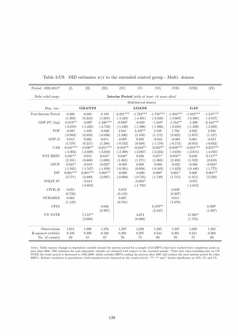
Table 3.C9: DID estimates w/r to the extended control group - Multi. donors.

Period: 1992-2015* (I) (II) (III) (IV) (V) (VI) (VII) (VIII) (IX)

Debt relief stage: Interim Period [with at least +6 years after]

Multilateral donors

Dep. var.: GRANTS LOANS GAT

Post-Interim Period 0.266 0.082 0.193 -2.221*** -1.722*** -1.758*** -1.934*** -1.582*** -1.547***(1.392) (0.334) (1.005) (-4.428) (-4.491) (-3.349) (-3.605) (-3.388) (-2.847)

GDP PC (log) -0.813** -0.897 -1.328*** -0.838* -0.659 -1.243* -1.554** -1.390 -2.444***(-2.019) (-1.235) (-2.743) (-1.849) (-1.206) (-1.986) (-2.059) (-1.339) (-2.933)

POP -0.081 1.239 -0.036 2.041 3.432** 2.108 1.794 3.922 2.358(-0.094) (0.859) (-0.036) (1.336) (2.103) (1.112) (0.925) (1.657) (1.127)

GDP G 0.012 0.002 0.011 -0.007 0.005 -0.016 -0.003 0.001 -0.011(1.578) (0.211) (1.286) (-0.532) (0.638) (-1.178) (-0.174) (0.054) (-0.642)

CAB -0.041*** -0.038** -0.051*** -0.018** -0.016** -0.022** -0.059*** -0.054*** -0.072***(-3.304) (-2.608) (-3.622) (-2.298) (-2.067) (-2.234) (-3.658) (-2.815) (-4.010)

TOT RESV 0.031** 0.012 0.044* 0.048* 0.036 0.071* 0.076** 0.049 0.117**(2.101) (0.600) (1.698) (1.865) (1.271) (1.888) (2.403) (1.522) (2.610)

GFCF -0.021* -0.018 -0.022* -0.003 0.008 -0.004 -0.022 -0.008 -0.024*(-1.945) (-1.547) (-1.856) (-0.301) (0.638) (-0.445) (-1.633) (-0.446) (-1.775)

INF 0.001*** 0.001*** 0.001** -0.000 -0.000 0.000* 0.001* 0.000 0.001**(2.771) (2.890) (2.097) (-0.608) (-0.725) (1.749) (1.715) (1.251) (2.520)

POLIT IV -0.014 -0.058* -0.071(-0.634) (-1.750) (-1.612)

CIVIL R 0.051 0.019 0.039(0.728) (0.145) (0.307)

DURABLE 0.004 0.007 0.011(1.129) (0.781) (1.078)

CPIA 0.048 0.479** 0.508*(0.397) (2.447) (1.887)

UN VOTE 7.112** 4.674 11.091*(2.089) (0.960) (1.752)

Observations 1,651 1,098 1,376 1,507 1,028 1,285 1,507 1,028 1,285R-squared (within) 0.195 0.200 0.192 0.295 0.207 0.344 0.261 0.211 0.302

No. of country 83 81 87 76 75 80 76 75 80

Notes: Table exposes changes in dependent variable around the interim period for a sample of 24 HIPCs that have reached their completion point nolater than 2009. DID estimates for each dependent variable are obtained with respect to the extended sample. *Note that when including data on UNVOTE the study period is shortened to 1992-2008, which excludes HIPCs ending the process after 2007 and reduces the post-interim period for otherHIPCs. Robust t-statistics in parentheses (with standard-erros clustered at the country-level). ***, ** and * denote significance at 10%, 5% and 1%.

138

Table 3.C10: Investigating heterogeneity in HIPCs’ market access.

(I) (II) (III) (IV) (V) (VI) (VII) (VIII) (IX) (X) (XI) (XII)

Debt relief stage: Interim Period [with at least +6 years after]

Dep. var.: PRIV BK PRIV CR PRIV CO

VAR: GDP PC RES RENT DURABLE HAIRCUT GDP PC RES RENT DURABLE HAIRCUT GDP PC RES RENT DURABLE HAIRCUT

Narrow CGPost-IP 2.587* 0.820** 0.857** 0.696** -1.462 1.367* 0.096 0.366 -7.378 2.652** 0.262 0.479

(1.697) (2.208) (2.547) (2.590) (-0.406) (1.850) (0.122) (0.465) (-0.937) (2.344) (0.234) (0.401)Post-IP*VAR -0.241 0.012 0.012 0.509* 0.387 -0.019 0.094** 1.323* 1.393 -0.058 0.150** 2.502*

(-1.160) (0.660) (0.966) (1.804) (0.724) (-0.627) (2.084) (1.870) (1.206) (-0.971) (2.405) (1.700)

Observations 593 593 593 593 593 593 593 584 593 593 593 593

Extended CGPost-IP 1.349 1.347*** 0.850** 0.958*** -9.839* 3.433*** 0.140 2.049 -16.090* 3.980*** -0.080 1.631

(1.056) (3.290) (2.571) (3.273) (-1.717) (2.689) (0.136) (1.646) (-1.958) (3.065) (-0.064) (1.086)Post-IP*VAR -0.015 -0.007 0.033* 0.524 1.909** -0.044 0.224*** 1.447 2.887** -0.067 0.262*** 2.642

(-0.082) (-0.507) (1.933) (1.607) (2.139) (-0.833) (2.971) (1.139) (2.363) (-1.298) (3.217) (1.462)

Observations 1,433 1,433 1,433 1,433 1,433 1,433 1,433 1,433 1,433 1,433 1,433 1,433

African CGPost-IP 3.451** 1.664** 1.145** 1.317** -1.100 2.593*** 1.002 1.967** -6.060 3.684*** 0.309 1.368

(2.538) (2.633) (2.297) (2.367) (-0.331) (3.094) (1.041) (2.067) (-0.821) (3.556) (0.232) (1.031)Post-IP*VAR -0.293 -0.014 0.028 0.329 0.561 0.004 0.132** 1.240 1.294 -0.092 0.181*** 2.198

(-1.534) (-0.869) (1.250) (0.938) (1.097) (0.105) (2.472) (1.499) (1.211) (-1.501) (2.915) (1.529)

Observations 585 585 585 585 585 585 585 585 585 585 585 585

Notes: Each regression includes the set of control variables used so far. F-stat are not reported (as well as intercepts) in order to save space but are all significant at the 1% level. Robust t-statistics inparentheses (with standard-errors clustered at the country-level). ***, ** and * denote significance at 10%, 5% and 1%.

139

Chapter 4

Taxation, Infrastructure, and Firm

Performance in Developing Countries

with Lisa Chauvet

4.1 Introduction

Since the early 1960s, there has been growing tendency to see the domestic resource

mobilization as a stepping stone for economic development. The impressive work undertaken in

recent decades to understand the determinants of taxation and its impact on economic activity has

helped policymakers design tax policies in both advanced and developing economies. Yet although

the need for further analysis of taxation and development has never let up, interest in these

issues by policymakers and scholars has fluctuated considerably. Although the improvement of

taxation in low-income countries (LICs) was among the commitments signed by the international

community at the Monterrey Conference in 2002, the contribution of taxation to financing the

Millennium Development Goals was overshadowed by the strong emphasis on the critical role that

foreign aid had to play. In addition, the aid effectiveness dispute of the 2000s and the growing

attention to remittances detracted from debates on domestic revenue mobilization. All this has

dramatically changed over the past few years. The public finance crisis in advanced economies

and the need for greater autonomy in financing for development have placed taxation issues

firmly on the development agenda. The June 2015 International Conference on Financing for

Development in Addis Ababa brought the question of taxation back to center stage: it reasserted

the decisive role of domestic revenue in helping developing countries to grow, and highlighted

the need to raise the level of taxes collected given the ambitious sustainable development goals

for 2030 and the budgetary constraints faced by traditional donors.

This call from the international community to improve domestic resource mobilization

was accompanied by renewed interest from academics and policymakers in improving their

understanding of how taxation can affect economic development, especially in countries with

substantial financing needs. Our paper investigates the effects of tax revenue on economic growth

in developing countries taking a micro approach and focus on their firms’ performance. In this,

the article sets out to contribute to the literature on taxation and firm growth, as yet very thin

141

on the ground when it comes to developing countries.

As recently shown in paper by Aghion et al. (2016), the effect of taxation on firm performance

can be twofold. On the one hand, taxes can be seen as a disincentive to innovate or invest

since one additional dollar of tax is one dollar that is not used for a production activity. This

first view is put forward by the large body of theory that builds on neo-classical models of

investment (Jorgenson, 1963; Tobin, 1969; Hayashi, 1982) and posits that taxation is harmful

for firm and industry development since it tends to negatively alter firm investment decisions

(Hall and Jorgenson, 1967; Summers et al., 1981; Auerbach et al., 1983). Empirical analyses

testing these theoretical predictions in advanced economies find that taxation does indeed depress

capital accumulation (Cummins et al., 1996), the firm growth rate (Carroll et al., 2001) and

entrepreneurship when tax progressiveness is too high (Gentry and Hubbard, 2000).

Yet on the other hand, tax resources are essential in financing the public infrastructures

key to corporate activity. Aghion et al. (2016) argue that the overall effect of taxation on firm

performance depends on the relative weight of these two effects, which can be very different

depending on the kind of country studied. This condition was initially stated by Barro (1990),

who argues that the effect of government spending (and hence taxes since he considers that

public finances are balanced) on economic growth depends on the size of the government and

especially on the marginal returns of public spending. According to him, a tax increase lowers

the growth rate of the economy while the resulting government spending raises it. Yet this second

effect dominates only when the government’s size is small (i.e. when the ratio of public finance

to the GDP is low). If the government is large, then the marginal returns of public spending

decrease and the negative tax effect dominates, slowing down GDP growth. Furthermore, as

pointed up by both Aghion et al. (2016) and Goyette (2015), the sound use of taxes in financing

infrastructure is a necessary condition for the existence of such a positive effect, which depends

heavily on the incidence of corruption within the country, and on the government’s political

accountability and willingness to invest domestic resources in promising projects for corporate

activity.

If most studies to date have found that taxation is bad for corporate activity, it may be

because they focus on advanced economies where the level of public infrastructures is already

satisfactory and the marginal effect of taxation therefore only represents a direct cost for

corporates. In keeping with the idea put forward by Aghion et al. (2016), in these countries,

the first negative effect hence outweighs the second positive effect. Yet looking at the impact

of taxation on firm activity in developing countries can produce different conclusions since the

lack of infrastructure in these countries really does hamper business development. A number of

studies find that infrastructure needs are a major impediment to economic growth in developing

countries, especially LICs (Collier and Gunning, 1999; Bigsten and Soderbom, 2006; Dollar

et al., 2005; Aterido et al., 2011; Harrison et al., 2014). Figure 4.A1 in the Appendix illustrates

the relationship between economic development and infrastructure and clearly shows that

infrastructure is considered as greater obstacle in poorer countries than in advanced economies.

This suggests that taxes in LICs could have a large positive effect on firm activity by means of

financing public infrastructure, subject to the condition that public revenue is indeed used for

such purposes and not diverted into corruption.

142

To our knowledge, the only studies that set out to observe the impact of taxation on economic

activity in developing countries are Easterly and Rebelo (1993), Djankov et al. (2010), Fisman

and Svensson (2007), and Goyette (2015). However since the first two remain at the country-level,

and the third considers the specific case of Uganda, the study by Goyette (2015) is the only

one that focuses on the average effect of taxation on firm performance in LICs. Although this

paper argues that, on average, taxation positively affects firm growth, the author uses firm-level

data on sales declared for tax purposes as a proxy for the effective tax rate and does not look

specifically at the channels through which taxation benefits firm activity. The purpose of our

paper is to use country-level tax variables to see how domestic revenue mobilization taken as a

whole (not just considering tax revenue on corporate profits) affects individual firm performance,

and what are the transmission channels for these effects.

We therefore examine the ability of taxes to affect firm growth and attempt to control for

the way these domestic resources are used. We use micro data on formal firm performance from

the World Bank Enterprise Surveys (WBES) (World Bank, 2015) on 57 countries (including

48 developing countries) covering the period from 2006 to 2015.1 These surveys have been

standardized over time and across all countries, allowing for repeated cross-sectional analysis.

We combine data on firm growth with tax data from the Government Revenue Dataset (GRD -

ICTD/UNU-WIDER), which provides the most reliable data on taxes to date with its impressive

coverage (across countries and over time) and level of disaggregation for domestic revenue

(Prichard et al., 2014).

Estimation of the impact of taxation on economic performance can be subject to a number

of estimation biases. The first source of bias is due to omitted variables: unobservable country

characteristics may explain variations in both firm growth and tax ratio. We thus include

numerous control variables in our estimations, both at the country and the firm- level, as well as

country and sector-year fixed effects in order to reduce the omitted variable bias. The second

source of bias is reverse causality. In well-performing countries with significant annual GDP

growth, an increase in GDP and consequently in the tax base is likely to improve the amount

of taxes collected. Yet although reverse causality is indisputable at the macro level, one firm’s

performance is hardly likely to affect the tax-to-GDP ratio at the country level, however large

the firm may be. Nonetheless, our empirical strategy leaves the possibility open for potential

simultaneity in our variables of interest since we estimate the effect of taxation on firm growth

within countries. Therefore, we may be capturing an average country-level relationship between

firm performance and taxation, in which case reverse-causality may still be an issue. In addition,

and over the past few years, it has been shown that a few large firms might significantly affect

the aggregate economic developments in the context of “granular” economies (Gabaix, 2011;

Di Giovanni and Levchenko, 2012; Di Giovanni et al., 2014). Although these findings are mostly

derived from studies based on high income countries, such feedbacks from micro to macro could

also be observed in developing countries, thus raising reverse causality issues as well. These

1The WBES cover more than 130 countries. Since our baseline specification consider within country variationand our IV strategy does not allow for the inclusion of small islands in our sample, we remove one-survey countriesand islands permanently from all the other tests. As explained in the Appendix B (p.177) the inclusion ofone-survey countries does not bring any information about the relationship we investigate. Moreover, consideringsmall islands with at least two enterprises surveys does not alter the results. We also drop Angola and Kazakhstan,which we consider as outliers. Indeed, including them tends to overestimate the impact of taxation on firm growth.

143

potential problems are discussed in the next section. Moreover, other sources of endogeneity

are likely to bias the estimates. In our model, time-varying unobservable heterogeneity is only

accounted for at the industry level and not at the country level. We therefore provide two-stage

least squares estimates in which the tax variable is instrumented by the level of taxation and

rent from natural resources in neighboring countries. Nevertheless, post-estimation tests suggest

that the endogenous feature of our variable of interest, tax revenue, is of little concern in this

study.

Across our global sample of 57 countries (including both developed and developing countries),

our results find no significant linear effect of the overall tax burden on firm growth. However

the relationship between taxation and firm growth appears to be non-linear and conditioned by

several factors, particularly by the level of development. We observe significant non-linearity

between taxation and firm growth with respect to the level of per capita GDP. While the marginal

effect of taxation is positive and quite large for lower levels of development, explicable by the

need for public infrastructures, it is negative and significant for firms operating in countries

with higher levels of income. In addition, the positive effect of taxation on firm growth in LICs

appears to be influenced by the level of corruption. Our results show that when the incidence of

corruption is high, the positive impact of taxation on firm growth is largely reduced, confirming

the findings of Aghion et al. (2016) and Goyette (2015). This indirectly suggests that the positive

contribution of taxation to corporate activity channels goes through the provision of public

goods and that, where there is a high level of corruption, taxes collected are not redirected to

infrastructure financing and hence merely represent an additional cost for firms. In the same

vein, we assume that non-resource taxes are more likely to increase government accountability

towards the general public than resource taxes, which can be considered as a rent and therefore

do not automatically imply public good counterparts. Using the Government Revenue Dataset

(GRD) which differentiates natural resource taxes from non-natural resource taxes, our results

find that the positive effect of taxation on firm performance is indeed driven by non-resource

taxes.

Lastly, we use an empirical specification similar to Rajan and Zingales (1998) to examine

the channels through which taxation positively affects firm growth in developing countries.

This specification includes interaction terms between taxation and an exogenous measure of

infrastructure intensity at the sector level derived from an input-output matrix of a frictionless

market. We find marginal evidence that the positive effect of taxes on firm growth is greater for

firms in industries that disproportionately depend on public utilities such as transport, electricity

and water supply. This last result hence points up public infrastructure as one of the potential

channels through which taxation benefits firm activity.

The rest of this paper proceeds as follows: Section 2 presents our empirical strategy and the

data used. Section 3 presents the baseline results and some robustness checks. Section 4 examines

how corruption alters the impact of taxation on firm performance. Using sector-specific intensity

measures, Section 5 then investigates the infrastructure channels through which domestic resource

mobilization potentially benefits firm growth. Section 6 concludes.

144

4.2 Model and Data

We use World Bank Enterprise Survey (WBES) repeated cross-section data on formal firm

performance over the 2006-2015 period to examine the impact of taxation on firm growth.2 The

WBESs cover a representative sample of firms in the manufacturing and service sectors for each

country, and are comparable across countries and years. Table 4.B1 in the Appendix B (p.178)

presents the sample of countries considered for this study, the number of firms interviewed per

country, and the year of the surveys. We use these data, to estimate the following general model:

GROWTHi,k,j,(t,t−2) = α+ βTAXj,(t,t−2) + λXi,k,j,t + γYj,(t,t−2) + µj + τk,t + εi,k,j,t (4.1)

where GROWTHi,k,j,(t,t−2) is the annual average growth rate in sales for firm i in industry

k in country j over the period (t, t-2).3 The sales in local currencies are deflated using the

GDP deflator (with the same base year of 2005 for every country) and then converted into

US dollars.4 Our main variable of interest is TAXj,(t,t−2), which is the share of total taxes,

excluding social contributions, in GDP. It is measured at the country level and on average over

the period for which sales growth is computed (t, t-2). We use the Government Revenue Dataset

(ICTD/UNU-WIDER) to measure total taxes. The GRD covers information on tax revenue

collected by both central and general government. Central government data are more widely

available, but as noted by Prichard et al. (2014), could be misleading for federal states with

more local taxes. Our rule of thumb is therefore to use general government taxes for a given

country whenever the number of observations is as high as for central government taxes. This

is the case with half of the countries included in the full sample. Otherwise, central level data

are used. In all regressions the country fixed effects, µj , account for whether general or central

government data are used.5

Our model controls for Xi,k,j,t, a set of firm-level characteristics. We include lagged sales,

SALESi,k,j,t−2 in order to account for catching-up effects. This variable captures the fact that

the smaller the past growth rate, the greater the prospects of higher growth in the future. In

keeping with Harrison et al. (2014), we control for the size of the firm, SIZEi,k,j,t, which takes

the value one if the firm employs less than 20 persons, two if the firm employs between 20

and 100 persons, and three for the largest firms (more than 100 employees). We also include

two variables accounting for the firm’s ownership structure: STATEi,k,j,t which is equal to

one if the state owns part (or all) of the firm, and FOREIGNi,k,j,t which is equal to one if

a foreign entity owns part (or all) of the firm. We also control for EXPORTi,k,j,t, which is

equal to one if the firm is outward-looking, i.e. if part of its production is exported directly or

indirectly (supplied to exporting firm). Lastly, the firm-level set of control variables includes

WEBSITEi,k,j,t, which is equal to one if the firm has a website. This variable is a proxy for

the firm’s access to a telecommunications infrastructure and has been shown by Harrison et al.

(2014) as key in explaining firm growth, especially in Africa.

2Version of November 11th 2015.3In each survey, firm sales are measured in t, which is the last fiscal year before the year the survey was

conducted, and in t-2 which is three fiscal years before the survey was conducted.4Data for the GDP deflator and the exchange rate come from the World Development Indicators database.5A dummy variable that is equal to one when general government data are used (GENGOVj) cannot be

estimated given that it does not vary over time.

145

At the country level, Yj,(t,t−2) includes the size of the country, POPULATIONj,(t,t−2),

in logarithm and on average over the period (t, t-2). We also account for the countries’

level of development using the logarithm of per capita income in constant 2005 US dollars,

INCOMEj,(t−3,t−5). To avoid endogeneity issues, this variable is lagged by one period, and

thus averaged over the (t-3, t-5). We also control for a corruption indicator to capture the

quality of institutions at the country level. The WBES provides information on how pervasive

corruption is perceived by firms. This variable ranges on a scale from 0 (corruption is not

perceived as an obstacle to current operations) to 4 (corruption is perceived as a very severe

obstacle to current operations). CORRUPTIONj,t is the re-aggregation at the country-level of

the firm-level perception of corruption. We use the firm probability weights provided by the

WBES to compute the mean value of corruption at the country- level.

Considering equation (1), one can see that including country-fixed effects leads our coefficient

of interest (β) to capture the contribution of changes in tax revenue to changes in firms growth

within country. Therefore, since our variable of interest is observed at the country-year level, we

need to have at least two surveys per country in order to observe changes in tax revenue. Indeed,

as discussed in the Appendix B (p.177), keeping countries with one round of WBES into our

sample of study artificially adds zeros to the taxation variable once the within transformation

is achieved. We thus intentionally omit one-survey countries which leads to only consider 57

countries out of 102 available in the WBES.6 Table 4.1 shows the summary statistics for the

sample of developing countries and low and lower-middle income countries (LICs/LMICs).

The annual average sales growth of formal firms is around 14.5% for the sample of developing

countries, and slightly less for LICs/LMICs, at approximately 12.5%. In these countries, some

20% of the firms are outward-looking, i.e. exporting part of their production either directly

or indirectly. This proportion is slightly higher for the sample of developing countries (around

25%). The firms operating in LICs/LMICs tend to have less access to the Internet as proxied by

WEBSITEi,k,j,t. In the other areas (state or foreign ownership, initial sales and size), the two

samples of firms are fairly similar.

At the country level, Table 4.1 suggests that corruption is pervasive with an average value of

around 1.7 on a scale from 0 to 4. The country-level variation is quite high, however, since some

countries return a maximum value of 2.9 (corruption is perceived as a major obstacle at the

country- level), and others a minimum value of 0.2 (corruption is not perceived as an obstacle at

all). Lastly, the share of taxes in GDP is quite low in our sample of developing countries (16.2%)

and even lower for LICs/LMICs (14.3%). Figures for tax revenue and natural resource rents in

neighboring countries will be discussed in the next sections of the paper.

6Preliminary version of this paper includes the entire sample of countries (102, of which 89 are developingcountries). Results do not change, but their interpretation thus becomes relevant only for countries with at leasttwo rounds of WBES.

146

Table 4.1: Summary statistics.

Variables mean sd min max mean sd min max

Firm characteristics

ALL DCs (N = 36,912 ) LICs/LMICs (N = 21,349)

GROWTHi,k,j,(t,t−2) % 14.556 72.116 -100 915.085 12.584 76.529 -100 915.085

SALESi,k,j,t−2 logarithm 12.874 2.654 2.056 28.622 12.312 2.852 3.203 27.279STATEi,k,j,t dummy 0.014 0.117 0 1 0.013 0.113 0 1FOREIGNi,k,j,t dummy 0.109 0.311 0 1 0.104 0.305 0 1EXPORTSi,k,j,t dummy 0.251 0.433 0 1 0.201 0.401 0 1SIZEi,k,j,t 1.683 0.801 0 3 1.606 0.781 0 3WEBSITEi,k,j,t Dummy 0.431 0.495 0 1 0.313 0.463 0 1

Country characteristicsa

ALL DCs ( N = 97) LICs/LMICs ( N = 61 )

INCOMEj,(t−3,t−5) logarithm 7.138 1.090 5.013 8.971 6.471 0.767 5.013 7.944

POPULATIONj,(t,t−2) logarithm 16.198 1.284 13.333 18.986 16.353 1.190 13.428 18.986

CORRUPTIONj,t 1.713 0.717 0.189 2.985 1.785 0.747 0.189 2.871TAXj,(t,t−2) %GDP 16.211 5.810 4.807 31.486 14.376 5.250 4.807 27.730

TAX NEIGHBj,(t,t−2) %GDP 16.295 4.226 6.607 27.366 14.545 3.753 6.607 24.143

NRR NEIGHBj,(t,t−2) %GDP 12.044 7.901 0.938 34.942 13.929 8.115 1.996 34.942

Notes: a Number of observations at the country level. Firm-level variables are from the World Bank Enterprise Surveys(various years). Data at the country level are from the World Development Indicators, except for CORRUPTION(weighted mean of the WBES at the country level) and TAX (GRD - UNU-WIDER/ICTD). Authors’ computation.

4.3 Baseline results

We first estimate equation 4.1 for the full sample of countries, including all 57 developing and

developed countries. Equation 4.1 is estimated using the OLS estimator and the firm probability

weights provided by the WBES. In keeping with Moulton (1990) and Froot (1989), the standard

errors are clustered at the country-year level (which is the level for our variable of interest,

TAXj,(t,t−2)). Column (I) of Table 4.2 presents the results. Across the full sample, we find

evidence of a catching-up effect both at the firm and country levels, as suggested by the signifi-

cantly negative coefficients of INCOMEj,(t−3,t−5) and SALESi,k,j,t−2. Firms in less developed

countries and with lower past performance tend to have higher growth prospects. Results also

suggest that foreign ownership is correlated with higher growth, as well as outward-looking

operations. Larger firms and firms with good telecommunications access also tend to grow faster.

As regards the effect of taxation on firm growth, regression (I) in Table 4.2 displays a positive

coefficient for TAXj,(t,t−2), although this is not statistically significant.

This absence of linear relationship between taxation and firm growth for our overall sample

of 57 countries may be due to the large country heterogeneity within the sample. Indeed, the

impact of taxes on firm performance has to be compared to the marginal effectiveness of taxes

147

to provide the economic environment conducive to growth. In that sense, the marginal effect of

taxes on firm growth may be greater when the scope for public goods provision is extremely high,

which is the case when the level of development is low (see Figure 4.A1 in the Appendix, p.170).

In highly developed countries with fair public goods provision, the marginal effect of taxation

may be lower and tax might represent a burden weighing on firms’ profitability and performance.

In order to examine the heterogeneity of the tax impact depending on the country’s level of

development we include, in regression (II) of Table 4.2, an interaction term for TAXj,(t,t−2) with

INCOMEj,(t−3,t−5).

The interaction term is significantly negative, in line with the idea of a marginal decreasing

impact of taxation with the level of development. The turning point in INCOMEj,(t−3,t−5), for

which taxation shows negative returns is around 4,700 USD per capita, which is the level of

development of a country such as Uruguay or Botswana in our sample (both have per capita GDP

of around 5,000 USD). Of the 57 countries in the full sample, 14 (corresponding to 14,178 firms,

which represents around 30% of our entire sample) display higher levels of income per capita.

This result is in line with the findings of Aghion et al. (2016) and the theoretical predictions of

Barro (1990) since above a certain level of development/or government’s size, the negative effect

of taxation on firm’s incentive to innovate and invest outweighs the benefits of public goods

provision. Columns (III) and (IV) of Table 4.2 confirm this result. The share of taxes in GDP

appears to be negatively correlated with firm growth in developed economies, while positively

correlated with firm growth in developing countries in which the prospects for improvements

in public goods provision are greater.7 Among the developing countries, however, the effect of

TAXj,(t,t−2) appears to be driven mostly by the low income and LMICs, as shown in regressions

(V) and (VI) of Table 4.2.

Yet sales growth may be influenced by factors that do not necessarily reflect firm structural

performance. Sales may be affected by aggregate demand dynamics and by the international

business cycles. Our model includes industry-year dummies which is a way to account for the

variation in firm’s sales that does not pertain to the firm performance per se. An alternative

way to measure firm performance is with labor productivity or even better, with total factor

productivity, TFP. The WBES has recently produced estimates of TFP but these are only

cross-sectional data, which would preclude using country and industry-year dummies. Labor

productivity can easily be computed on our sample of countries and years, as well as its growth

rate. However, given that our specification includes the size of the firm on the right-hand side,

we expect the results to be very similar if sales growth is replaced with productivity growth.

This in indeed confirmed in Table 4.A1 in Appendix (p.172). We re-estimate our benchmark

results on labor productivity growth. On the right hand-side initial sales, SALESi,k,j,t−2, is

replaced with initial labor productivity, PRODi,k,j,t−2. We find results which are similar to

those presented in Table 4.2.

7Figures for non-developing countries have to be considered carefully given the small number of “developed”economies in this sub-sample (9) and the few resulting observations at the country-year level (only 16).

148

Table 4.2: Baseline estimations of the impact of tax on firm growth.

(I) (II) (III) (IV) (V) (VI)

Dep. var.: GROWTHi,k,j,(t,t−2)

Sample: All countries Non-DCs DCs

Sub-samples: All LICs/LMICs UMICs

Taxation var.TAXj,(t,t−2) 1.327 14.414*** -3.064** 4.359*** 3.238** 2.164

(1.11) (5.17) (1.39) (1.07) (1.41) (2.21)TAX * INCOMEj,(t,t−2) -1.706***

(0.63)

Country-level control var.CORRUPTIONj,t -4.155 -6.415 -0.278 -7.812 6.647 -8.327

(5.06) (5.13) (4.52) (5.74) (9.89) (7.12)INCOMEj,(t−3,t−5) -102.229*** -65.143** -81.639** -93.716*** -23.697 -46.861***

(24.71) (27.97) (29.54) (31.38) (42.73) (9.32)POPULATIONj,(t,t−2) 83.730* 68.790* 138.527 105.663* -19.237 597.554***

(43.04) (41.26) (120.24) (54.00) (66.26) (71.29)Firm-level control var.SALESi,k,j,t−2 -16.980*** -16.981*** -21.353*** -14.517*** -13.012*** -15.668***

(1.96) (1.96) (4.28) (1.62) (1.88) (2.65)STATEi,k,j,t 1.859 1.899 -10.188 8.583 18.675 2.967

(7.91) (7.92) (10.79) (8.57) (16.52) (10.27)FOREIGNi,k,j,t 10.239** 10.322** 18.736* 4.045 8.623** -1.148

(4.87) (4.86) (9.43) (3.62) (4.04) (5.37)EXPORTi,k,j,t 7.952*** 7.947*** 8.210 8.315** 5.284* 10.496**

(2.91) (2.91) (5.58) (3.31) (2.98) (4.88)SIZEi,k,j,t 26.358*** 26.328*** 31.041*** 23.611*** 22.807*** 24.441***

(3.23) (3.23) (7.36) (2.65) (3.61) (3.99)WEBSITEi,k,j,t 13.880*** 14.022*** 17.243*** 11.242*** 8.102*** 13.782**

(2.93) (2.94) (4.61) (3.46) (2.85) (5.14)

Constant -641.963 -615.101 -1,065.801 -1,088.310 609.032 -8,419.858***(795.31) (760.38) (1,948.63) (1,019.26) (1,236.97) (1,087.15)

Observations 44,703 44,703 7,791 36,912 21,349 15,563R-squared 0.207 0.208 0.220 0.209 0.214 0.229No. of countries 57 57 9 48 30 18No. of country-year obs. 116 116 19 97 61 36Country FE Yes Yes Yes Yes Yes YesSector-Year FE Yes Yes Yes Yes Yes Yes

Notes: The higher one percent of firms with the largest growth rates has been dropped from the sample. DCs stands for“Developing countries” and includes aid recipients only. OLS estimations using firm probability weights. Robust standard errorsin parentheses (clustered at the country-year level).***, ** and * denote significance at 10%, 5% and 1%.

When estimating the impact of taxation on growth outcomes, there are two main sources

of endogeneity bias: (1) reverse causality, which stems from the fact that the creation of wealth

in an economy influences the amount of taxes that can be raised; and (2) omitted variables,

due to the fact that growth performance and taxes can both be determined by the countries’

unobservable structural, historical and institutional characteristics. In the following, we try to

provide solutions to minimize these potential estimation biases.

149

4.3.1 Endogeneity concerns

Feedback from micro to macro

So far, our identification strategy has been based mainly on the introduction of country and

industry-year fixed effects and on the different levels of aggregation of the variable of outcome,

GROWTHi,k,j,(t,t−2), and of interest, TAXj,(t,t−2). The fact that TAXj,(t,t−2) is measured at

the country level, while GROWTHi,k,j,(t,t−2) is measured at the firm level, allays to some extent

reverse-causality concerns. We think it is indeed quite unlikely that the growth performance of

one firm, even a large one, would determine how much tax is raised in a country.

Yet, such assessment remains debatable since it has been shown that large firms could

significantly explain aggregate economic developments (the “granular hypothesis”), especially in

high-income countries (Gabaix, 2011; Di Giovanni and Levchenko, 2012; Di Giovanni et al., 2014).

In the context of developing countries where the size distribution of firms is highly skewed, the

IMF states as a recurrent theme that targeting properly the largest firms might secure around

60 to 80% of domestic taxes (and even more for small islands) (IMF, 2011),

In addition, moving back to the discussion about the sample restriction in the Appendix B

(p.177), the β coefficient in equation 4.1 mechanically captures a relationship between taxation

and the average firm growth rate at the country level when country fixed effects are included.

Under the “granular hypothesis”, it might thus be likely that the average firms growth (or

productivity growth), mostly derived from the largest firms, acts upon the country’s GDP growth,

and thus determines the amount of taxes collected. Hence reverse causality would be important

in this context, and mainly driven by firms observed at the tail-end of distribution.

Therefore, while to our knowledge their is no empirical evidence of such “granular hypothesis”

in the context of developing countries, we investigate whether the largest firms of the countries

considered for this study affect aggregate economic fluctuations, and in fine changes in the

tax-to-GDP ratio. Following Gabaix (2011), we thus test whether idiosyncratic movements of

the 5% (and alternately 10%) largest firms of each developing countries considered in the sample

(and averaged at the country-level), affect aggregate growth developments as well as taxation.

We perform this analysis using regression (IV) in Table 4.2 on the sample of developing countries

as our baseline result. To this end, we build the average idiosyncratic shock of the largest firms

(Γj,t) following Gabaix (2011) and use this measure to explain the country-level sales growth

rate, GDP growth, and tax-to-GDP ratio (see. Appendix C (p. 179) for the calculation of

idiosyncratic shocks).

Table 4.3 below shows the effect of largest firms’ idiosyncratic movements on aggregate

economic developments. Results support the absence of “granular hypothesis” meaning that

developments encountered by the largest firms have no effect on aggregate economic movements.

Indeed, the average idiosyncratic shock of either the 5% (Panel A) or 10% (Panel B) largest

firms in a given country, does not seem to explain the within-country variation of aggregate

growth nor taxation. Note that adding controls (both directly observed at the country-level or

at the firm-level and then aggregated at the country-level) does not alter the results. However,

conversely to Gabaix (2011), the composition of our sample is such that we have very few

time-variation (maximum 3 years) which probably explains why no effect is to be observed.

150

Nevertheless, the absence of correlation between the idiosyncratic movements of the biggests

firms and the aggregate country performance tends to be re-assuring regarding the potential

feedback from micro to macro that may be biasing our baseline results.

Table 4.3: Investigating the ”granular hypothesis” in developing countries.

(I) (II) (III) (IV) (V) (VI) (VII) (VIII) (IX)

Dep. var.: GROWTHj,(t,t−2) GDP Gj,(t,t−2) TAXj,(t,t−2)

Γ Measure Γ Γ bis Γ sect Γ Γ bis Γ sect Γ Γ bis Γ sect

Panel A - 5% largest firms

Γj,t 0.508 0.256 0.281 0.006 0.008 0.019 0.014 0.022 0.017(0.30) (0.30) (0.20) (0.03) (0.04) (0.02) (0.02) (0.02) (0.02)

Observations 97 97 97 97 97 97 97 97 97R-squared 0.798 0.740 0.751 0.778 0.778 0.783 0.970 0.970 0.970

No. of firms 5% 1698 1698 1698 1698 1698 1698 1698 1698 1698

Panel B - 10% largest firms

Γj,t 0.522* 0.411 0.310 0.007 -0.003 0.009 0.014 0.019 0.016(0.30) (0.43) (0.24) (0.03) (0.03) (0.03) (0.02) (0.02) (0.02)

Observations 97 97 97 97 97 97 97 97 97R-squared 0.800 0.756 0.747 0.778 0.777 0.778 0.970 0.970 0.970

No. of firms 10% 3451 3451 3451 3451 3451 3451 3451 3451 3451

Γ specification

Fixed effects C CxS CxSxY C CxS CxSxY C CxS CxSxYTime FE Yes Yes No Yes Yes No Yes Yes No

Firm-level controls Yes Yes No Yes Yes No Yes Yes No

Notes: GROWTHj,(t,t−2) denotes the average sales growth rate at the country-level (for country j, between t and t − 2).GDP Gj,(t,t−2) is the GDP growth rate of country j over the same time period. Lastly, TAXj,(t,t−2) represents the averagetax-to-GDP ratio (used in above regressions) for country j, between t and t− 2. Γ denotes the average idiosyncratic shock forlargest firms when idiosyncratic components of the productivity growth have been calculate with country fixed effects (C). Γ bis

is obtained from residuals derived from a specification where we replace country fixed effects with country-sector fixed effects(CxS). Lastly, Γ sect is based on residuals derived from a specification with country-sector-year fixed effects (CxSxY). Panel Areports results when the average idiosyncratic shock is based on the largest 5% firms, while Panel B when this measure is basedon the 10% largest firms. The higher one percent of firms with the largest growth rates has been dropped from the sample beforecollapsing the variables at the country-year level (using firm probability weights) and before computing the various Γ measures.Robust standard-errors in parentheses (cluster at the country level). ***, ** and * denote significance at 10%, 5% and 1%.

Omitted variable bias

Regarding the other potential sources of endogeneity, the introduction of country and

industry-year fixed effects in the baseline specification does not fully preclude an omitted variable

bias.

Regression (IV) in Table 4.2 on the sample of developing countries is our baseline result. In the

following, we provide robustness checks of this baseline estimation that address both confounding

151

factors and reverse-causality issues. First, we examine the robustness of the baseline result to

additional covariates. Given that TAXj,(t,t−2) is measured at the country level, the primary

source of omitted variable bias is likely to be at the country level. Panel A of Table 4.4 includes

country characteristics that may be correlated with both the tax ratio and firm performance. In

keeping with the existing literature on taxation in developing countries, we include variables that

have been shown as being major determinants of the domestic revenue mobilization (Agbeyegbe

et al., 2006; Crivelli and Gupta, 2014; Teera and Hudson, 2004; Bornhorst et al., 2009). We

include variables that account for internal determinants of taxation: a measure of institutional

quality, POLITYj,(t,t−2), the growth rate of the GDP (GROWTHj,(t,t−2)), and the share of

natural resource rent in GDP, NRRj,(t,t−2). In column (IV) of Table 4.4, we also include the tax

share squared in order to capture any non-linearity in the tax ratio rather than in development

level as we did in Table 4.2.

We also include external sources of financing that may substitute or complement taxation.

We test the robustness of our baseline by adding foreign direct investments (net inflows) in

percentage of GDP (FDIj,(t,t−2)). As underlined in Morrissey et al. (2016), we also include

imports (IMPORTSj,(t,t−2)) and exports (EXPORTSj,(t,t−2)) (both expressed as a share of

GDP) since both flows usually face different tariffs and tax regimes.8 Finally, we include foreign

aid as a share of GDP, AIDj,(t,t−2). This latter variable is introduced in a non-linear way to

capture the marginal decreasing returns in aid effectiveness (Hansen and Tarp, 2001; Lensink

and White, 2001). All these variables are downloaded from the World Development Indicators

(World Bank, 2016), except for foreign direct investment flows which have been retrieved from

the UNCTAD database (UNCTAD, 2016) and aid which was downloaded from the OECD-DAC

website.

Column (I) in Panel A of Table 4.4 replicates the baseline estimate for the sample of developing

countries. Columns (II) to (IX) in Panel A of Table 4.4 show that when the macroeconomic

covariates are sequentially introduced in the baseline OLS estimations, none of them is significant

with the exception of FDI —with an unexpected sign— and aid and its square term (jointly

significant, p-value = 0.027).9 In all columns, TAXj,(t,t−2) remains significantly positive and in

similar ranges (the coefficient ranges from 4.5 to 5.5). When we include the squared term of

TAXj,(t,t−2) in column (V), this additional variable is not significant, and TAXj,(t,t−2) becomes

marginally significant (p-value = 0.100).

Our second approach to deal with endogeneity concerns consists in estimating Equation 4.1

with the two-stage least squares estimator (TSLS). We use two instrumental variables, both

relying on the assumption that the tax ratio in country j is linked, through tax competition, to

the tax ratio of its neighboring countries n. Indeed, Lee and Gordon (2005) have shown that

tax rates between nearby countries are highly correlated, as illustrated in Figure 4.1. However,

it is fairly unlikely that the private sector activity of a given country affects the taxation of

its neighboring countries, which therefore makes the average tax ratio of the neighbors a good

instrument for this study. In addition, we also consider the average natural resource rents of

8We also included the share of trade (imports plus exports) in GDP, and found that this variable is notsignificant and does not alter the coefficient of taxation.

9The turning point in aid suggests that aid has a positive impact on firm growth for countries receiving lessthan 11% of their GDP in aid, which is in line with Chauvet and Ehrhart (2015).

152

neighboring countries as an instrument since variation in resource rent is induced mostly by price

fluctuations on international markets, and can directly affect the tax rate of the country (as

shown by Bornhorst et al. (2009), Thomas and Trevino (2013), and Crivelli and Gupta (2014)),10

and can consequently impact the tax rate of its neighbors under the tax competition argument.

So we define the first instrument as the average of the neighbors’ tax ratios (as a share of GDP),

TAX NEIGHBj,(t,t−2), and the second one as the average of the neighbors’ natural resource

rents (as a share of GDP), NRR NEIGHBj,(t,t−2). They are both obtained from:

TAX NEIGHBj,(t,t−2) = (1/Nj)ΣNn=1TAXn,(t,t−2) ×NEIGHBORj,n

NRR NEIGHBj,(t,t−2) = (1/Nj)ΣNn=1NRRn,(t,t−2) ×NEIGHBORj,n

where NEIGHBORj,n is a dummy variable equal to 1 if country n shares a land border with

country j (with Nj its total number of neighboring countries). Column (I) of Panel B of Table 4.4

displays the results. In this regression we use the same specification as in column (IV) of Table

4.2 with no additional covariates. The TSLS estimate is close to the OLS estimate in Panel A,

with a slightly higher coefficient for TAXj,(t,t−2).11 The first-step estimate is satisfactory, with

both instruments being significantly correlated with TAXj,(t,t−2) and displaying the expected

sign. The Hansen test for over-identification and Kleibergen-Paap F-Stat also suggest that the

instruments are valid.

One key condition for TAX NEIGHBj,(t,t−2) and NRR NEIGHBj,(t,t−2) to be valid

instruments is that they affect firm growth, GROWTHi,k,j,(t,t−2), solely through their impact

on TAXj,(t,t−2). This exclusion restriction may, however, be violated if the instruments affect

firm growth through other macroeconomic covariates, such as trade, for example. One way to

investigate the validity of the instruments and check for the exclusion restriction is to include in

the TSLS estimations the other potential channels through which the instruments may affect

firm growth. This test is performed in Panel B, regressions (II) to (IX) of Table 4.4. The results

suggest that the TSLS estimate of the coefficient of TAXj,(t,t−2) is unaltered by the introduction

of additional macroeconomic covariates. The first-step results remain largely unchanged, as do

the Hansen and Kleibergen-Paap F-Stat. In column (V), we also instrument tax rate squared,

with the squared expression of the two instruments.12 The instruments perform quite poorly, as

illustrated by the Hansen and Kleibergen-Paap F-Stat, which might explain why TAXj,(t,t−2)

records an unexpected large coefficient in column (V).

10Although it is less obvious as suggests Figure 4.1.11Although the OLS coefficient is not significantly different from the one obtained with the TSLS estimate since

their confidence intervals overlap.12The results are very similar when we remove the squared terms of the two instruments, although we slightly

lose in statistical significance.

153

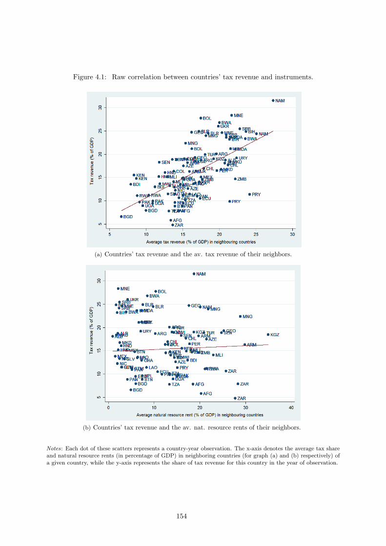
Figure 4.1: Raw correlation between countries’ tax revenue and instruments.

(a) Countries’ tax revenue and the av. tax revenue of their neighbors.

(b) Countries’ tax revenue and the av. nat. resource rents of their neighbors.

Notes: Each dot of these scatters represents a country-year observation. The x-axis denotes the average tax shareand natural resource rents (in percentage of GDP) in neighboring countries (for graph (a) and (b) respectively) ofa given country, while the y-axis represents the share of tax revenue for this country in the year of observation.

154

Table 4.4: Additional macroeconomic covariates and TSLS estimations.

Sample: DCs (I) (II) (III) (IV) (V) (VI) (VII) (VIII) (IX)Dep: var.: GROWTHi,k,j,(t,t−2)

VARIABLEj,(t,t−2) POLITY GROWTH TAX2 NRR FDI EXP IMP AID

Panel A OLS

TAXj,(t,t−2) 4.359*** 4.905*** 4.151*** 6.535 4.838*** 5.558*** 4.495*** 5.200*** 5.256***

(1.07) (1.05) (1.36) (3.95) (1.15) (0.96) (1.09) (1.28) (1.08)VARIABLEj,(t,t−2) 0.563 0.340 -0.055 -0.913 -1.800*** -0.387 -0.606 2.287

(1.05) (1.22) (0.09) (0.85) (0.51) (0.58) (0.54) (2.40)VARIABLE2

j,(t,t−2) -0.108**

(0.05)

Panel B TSLS

TAXj,(t,t−2) 6.624** 7.713*** 7.352 20.020** 7.289** 10.960*** 6.047** 7.223** 7.148**

(3.29) (2.76) (4.80) (7.95) (3.53) (3.99) (3.03) (3.46) (3.34)VARIABLEj,(t,t−2) 0.846 -0.425 -0.372* -1.225 -2.377*** -0.451 -0.889 2.708

(1.06) (1.90) (0.19) (1.10) (0.73) (0.58) (0.57) (2.61)VARIABLE2

j,(t,t−2) -0.123**

(0.06)First-step

TAX NEIGHBj,(t,t−2) 0.303*** 0.285*** 0.201* 0.556* 0.234** 0.267*** 0.314*** 0.291*** 0.275***

(0.09) (0.08) (0.10) (0.29) (0.10) (0.09) (0.099) (0.08) (0.09)NRR NEIGHBj,(t,t−2) -0.164** -0.226*** -0.166*** 0.004 -0.193*** -0.146** -0.201*** -0.129* -0.182***

(0.06) (0.06) (0.05) (0.13) (0.06) (0.07) (0.06) (0.07) (0.06)

F-Stat 1st Step (p-value) 0.000 0.000 0.000 0.000 0.000 0.000 0.000 0.000 0.000Kleibergen-Paap Wald F-Stat 14.53 19.92 9.62 8.91 12.56 8.61 16.56 12.86 17.63% bias included ≤ 15% =10% ≤ 20% ≤ 20% ≤ 15% ≤ 25% ≤ 15% ≤ 15% ≤ 15%Hansen J-Stat (p-val.) 0.548 0.945 0.560 0.106 0.908 0.569 0.643 0.440 0.747Hausman endog. (p-val.) 0.501 0.257 0.473 0.237 0.418 0.159 0.620 0.655 0.514

Observations 36,912 35,792 36,912 36,912 36,912 36,912 36,912 36,912 36,912No. of countries 48 48 48 48 48 48 48 48 48Country/Sector-Year FE Yes Yes Yes Yes Yes Yes Yes Yes Yes

Notes: The higher one percent of firms with the largest growth rates has been dropped from the sample. Panel A: OLS estimations usingprobability weights. Panel B: 2SLS estimations using firm probability weights. Robust standard errors (clustered at the country-year level) inparentheses.***, ** and * denote significance at 10%, 5% and 1%.

155

Table 4.4 thus suggests that when country-level confounding factors and reverse causality

are accounted for, the baseline results remain largely unchanged. However, Table 4.4 also reports

for each TSLS estimate the Hausman exogeneity test (its p-value). We observe that for each

TSLS estimate, the p-value associated with the Hausman test is larger than 0.05 which prevents

us to reject the null hypothesis under which the variable defined as endogenous (TAXj,(t,t−2)) is

actually exogenous.

Endogeneity concerns may also be raised regarding firm-level covariates. First, we check

whether the specification omits any firm-level variable that may be correlated with both firm

performance and the tax ratio. Thus, we investigate the robustness of the baseline result to the

inclusion of additional firm-level covariates. The results are presented in Panel A of Table 4.A2

in Appendix A (p.173). Again, column (I) replicates the baseline result. In column (II), we

control for whether the firm’s CEO is a female, using a dummy variable, as well as whether the

firm faces strong infrastructure obstacles, either electricity (column (III)) or transport obstacles

(column (IV)).13 Lastly, in column (V) we also add a dummy variable indicating whether the

firm has experienced power outages in the last fiscal year. Table 4.A2 shows that the coefficient

of TAXj,(t,t−2) is unaltered by the introduction of these additional firm-level covariates.

Second, we examine whether the potential endogeneity of firm-level controls affects the

estimated coefficient of TAXj,(t,t−2). One simple way to deal with firm-level control endogeneity

is to aggregate all the firm-level controls on cells at the sector-region level (Harrison et al., 2014).

Column (VI) of Panel A of Table 4.A2 displays the results when firm-level controls are aggregated

on these cells: the coefficient of TAXj,(t,t−2) is virtually unchanged. Lastly, we perform the same

test sets (including additional firm-level covariates and aggregating all the firm-level controls)

using the TSLS estimator. The results are displayed in Panel B of Table 4.A2. Including

additional firm covariates and aggregating the controls alter neither the TSLS estimate of the

coefficient of TAXj,(t,t−2) nor the validity of the instruments. Moreover, as for results reported

in Table 4.4, we note that p-values associated with Hausman tests all reject the endogenous

feature of our variable of interest. This let us think that the relationship between tax revenue

and the dynamism of formal firms’ activity in developing countries is not as straightforward as

one might thought.

The additional firm-level control variables in Table 4.A2 aim at capturing, as much as

possible, the time-varying observable heterogeneity in firm performance. In order to take into

account the time-invariant firm-level heterogeneity we also estimate the impact of TAXj,(t,t−2)

on firm performance measured for a sample of firms in 29 developing countries for which we have

two obervations in time. This estimation thus allows us to include a firm fixed effect into the

estimation.14 The estimations also include industry-year dummies and the standard errors are

clustered at the country-year level. Table 4.A3 (in the Appendix A, p.174) presents the results

when firm performance is measured either using sales growth, GROWTHi,k,j,(t,t−2), or labor

productivity growth, PRODUCTIV ITYi,k,j,(t,t−2). The coefficient of TAXj,(t,t−2) is negative

in columns (I) and (III) (and significant in column (III)) which is consistent with our baseline

results given that around half of the 29 countries for which we can perform these estimation are

upper middle-income countries. Consistenly with column (II) of our baseline Table 4.2, we thus

13Both electricity and transport variables range from 0 (low obstacle) to 4 (severe obstacle).14For a detailed presentation of the firm-level panel dataset, see Chauvet and Ehrhart (2015).

156

estimate 4.1 with firm panel data but include in columns (II) and (IV) an interaction term of

TAXj,(t,t−2) with the level of income per capita. In line with our previous conclusions, estimates

results suggest that the level of taxation is positively correlated with firm performance in low

and lower-middle income countries, for income per capita levels below 1,230 USD.

4.3.2 Further robustness checks

In Tables presented in Appendix D, we provide further robustness checks on the baseline

results. The first set of robustness checks consists in examining whether the results are altered

by the choice of the fixed effects introduced in equation 4.1. Panel A of Table 4.D1 in the

Appendix D (p.180) presents the coefficient for TAXj,(t,t−2) when the sector-year dummies are

replaced by sector and year dummies. The coefficients are very similar to those in Table 4.2,

with the exception that the average positive effect of taxation on firm performance for the overall

sample is now statistically significant at the 10% level. Panel B then re-estimates the same

specification as in the baseline (with sector-year dummies), but this time we change the level of

clustering. Instead of clustering the standard errors at the country-year level, we cluster them

at the country level. The significance of the coefficient of TAXj,(t,t−2) in column (IV) for the

sample of developing countries, is unaffected. Only the result for the full sample (column (I))

loses significance. Lastly, in Panel C, we examine robustness to a change in both the fixed effects

and the level of clustering. As in Panel A, the results are unchanged, except that the negative

effect of taxation on firm growth in advanced economies is now marginally significant (around the

10% level). Table 4.D1 (in the Appendix D, p.180) thus suggests that the estimated coefficient

of TAXj,(t,t−2) is robust to the kind of clustering and fixed-effects introduced, especially for the

sample of developing countries in column (IV).

The last set of robustness checks examines the issue of sample dependence, as well as

potential bias due to outliers. First, regression (IV) of Table 4.2 is re-estimated with each

regional sub-sample excluded (one at a time) in order to check that the baseline results are not

driven by one specific region. Table 4.D2 in the Appendix D (p.181) shows that the coefficient

of TAXj,(t,t−2) is again unaltered by these sample changes. Second, Table 4.D3 in the same

Appendix (p.181) re-estimates the baseline regression (IV) for Table 4.2 dropping one country at

a time. They both provide evidence that the coefficient of TAXj,(t,t−2) is unaffected when the

developing countries in the sample are excluded one at a time, suggesting that the results are

not driven by one specific country, or potential outliers. In the same vein, we alternately drop

sub-samples of firms belonging to each of the 21 sectors in our sample in order to see whether

results are driven by sector specific characteristics (although we control for sector fixed effects

and sector-year fixed effects in Table 4.D1). The results are presented in Table 4.D4 (Appendix

D, p.183) and highlight that, as with the previous robustness checks, the positive effect of

taxation on firm growth remains statistically significant and is not driven by a sub-sample of

firms operating in a more buoyant sector than the others.

Third, although we control for firm time-varying characteristics via the inclusion of firm-level

covariates, our benchmark result for the developing countries could potentially be driven by a

small cluster of firms presenting specific features. We consequently run estimate (IV) on Table

4.2, this time dropping sub-samples of firms based on a given feature. For instance, Panel B in

157

Table 4.D5 in the Appendix D (p.184) presents the results for our benchmark specification when

state-owned firms are dropped from the sample. Panel F does the same, excluding this time

small-size firms (with less than 20 employees). The results in Table 4.D5 show that the positive

effect of taxation on firm performance remains significant across all these different panels, and is

not driven by a specific type of firm.

Lastly, as illustrated by Table 4.B1 (p.178), the number of firms surveyed in each country

varies quite a lot depending notably on the level of development. Because our variable of interest

is measured at the country level, the unbalanced number of firms for the different countries

implies that some countries are over-represented in the sample of firms. To account for this

problem, we randomly draw, for each survey, sub-samples of firms (100 firms, 200 firms, and

300 firms), re-run the baseline estimation on these sub-samples (replicating the random draw

500 times), and compute the average coefficient for TAXj,(t,t−2), as well as the proportion of

regressions in which the coefficient is not statistically significant. Table 4.D6 in the Appendix D

(p.185) presents the results. We observe that starting from a draw of 200 firms, the coefficient of

TAXj,(t,t−2) is almost always statistically significant over the entire replication and stands, on

average, at around 3.4.

Overall, Tables 4.D1 to 4.D6 all suggest that the positive effect of the share of taxes in GDP

on firm growth in developing countries is robust to sub-sample estimations as well as to changes

in the specification of the fixed effects and in the level of clustering.

4.4 Taxation and Corruption Nexus

The main mechanism explaining how taxation can positively affect firm growth is that it is

used to provide public goods that are conducive to growth. These public goods are infrastructure

(electricity and transportation in the main), as well as education and health facilities conducive

to the effectiveness and social well-being of the labor force and ultimately capital accumulation.

In this section we provide indirect evidence that the positive effect of taxation disappears

when the conditions are not met for it to transform into public goods provision. We examine

two mechanisms that can prevent taxation from contributing to the provision of public goods:

(1) lack of government accountability; and (2) embezzlement by the political elite.

Government accountability is closely linked to its reliance on the taxation of citizens. With-

out taxation, any democracy would fail: taxation is what makes governments accountable to

the population. It has been shown in the literature that windfall finance tends to reduce the

accountability of governments to the citizens (Tsui, 2011). It has also been emphasized that

the impact of windfall finance, such as natural resource rents, on growth outcomes is more

adverse when institutions are weak (Mehlum et al., 2006). Lastly, natural resources also tend

to adversely impact the demand for accountability through the decrease in taxation that they

induce (Bornhorst et al., 2009; McGuirk, 2013; Crivelli and Gupta, 2014).

In the following, we examine whether all forms of taxation produce the accountability

effect that is required for taxation to transform into public goods provision. The Government

Revenue Dataset (ICTD/UNU-WIDER) provides information on whether taxation is raised from

non-resource sectors, NRTAXj,(t,t−2), or from the extraction of natural resources RTAXj,(t,t−2).

158

In line with the GRD glossary, resource taxes do not include royalties and other revenue from

exploitation rights. Resource taxes thus cover direct taxes on corporations operating in the

resource sector, and indirect resource taxes (such as excise duty on refined products for instance).

We therefore examine whether the positive effect of taxation holds when taxation stems from the

resource sector, which we assume does not discipline the government into providing public goods

to the population. Table 4.5 provides summary statistics on disaggregated taxes. The number of

country-year observations falls from 97 on the full sample of developing countries to 93. Despite

being a small part of all taxes, RTAXj,(t,t−2) in some countries represents almost 10% of GDP.

Yet Table 4.5 shows that, on average, resource taxes remain a minor source of revenue for the

countries in our sample.

Table 4.5: Summary statistics on disaggregated taxes.

Variable mean sd min max obs

All DCs

TAXj,(t,t−2) 16.211 5.810 4.807 31.486 97NRTAXj,(t,t−2) 15.631 5.715 4.807 30.537 94RTAXj,(t,t−2) 0.644 1.744 0.000 8.598 93

Table 4.6 presents the results when the TAXj,(t,t−2) variable we have used so far is

divided into non-resource taxes, NRTAXj,(t,t−2), and resource taxes, RTAXj,(t,t−2). The first

column of Table 4.6 reproduces our baseline result in column (IV) of Table 4.2. Column (II)

then estimates the same regression on the sample of countries for which we have information

on the resource and non-resource components of taxation. The TAXj,(t,t−2) coefficient remains

positive, statistically significant, and in the same magnitude as the benchmark coefficient. In

column (III), we disaggregate between resource and non-resource taxation.

The results suggest that only the non-resource taxes display a positive correlation with

firm growth. Taxes raised from the resource sector are not significantly associated with firm

outcome. These results hence suggest that when taxation is not associated with some form of

government accountability to the citizens, as is likely to be the case when taxation stems from

natural resources, then the positive effect of taxation disappears. This finding is in line with the

idea that the positive impact of taxation on firm growth stems from the public goods provision

that it entails.

159

Table 4.6: Impact on growth of resource and non-resources taxes.

Sample: DCs (I) (II) (III)

Dep. var.: GROWTHi,k,j,(t,t−2)

TAXj,(t,t−2) 4.359*** 4.292***(1.07) (1.21)

NRTAXj,(t,t−2) 3.683***(1.11)

RTAXj,(t,t−2) -2.036(3.18)

Observations 36,912 35,947 35,947R-squared 0.209 0.209 0.210No. of countries 48 48 48Country-level var. Yes Yes YesFirm-level var. Yes Yes YesCountry FE Yes Yes YesSector-Year FE Yes Yes Yes

Notes: The higher one percent of firms with the largestgrowth rates has been dropped from the sample. OLS esti-mations using firm probability weights. Robust standard-errors clustered at the country-year level in parentheses.***, ** and * denote significance at 10%, 5% and 1%.

The second mechanism that we examine is embezzlement by the political elite. This

mechanism has already been evidenced by Aghion et al. (2016) using US data and by Goyette

(2015) for a small sample of developing countries. Corruption generally diverts public resources

from their purpose, namely the provision of public goods. If taxation has a positive impact on

firm growth that stems from the provision of public goods, then this requires that corruption is

not too pervasive. In Table 4.7 we examine the relationship between taxation, corruption, and

growth by introducing an interaction term between the taxation variable and the corruption

variable. We use two measures of corruption, both re-aggregating at the country-level information

provided in the WBES.15 The first measure is the perception of corruption as an obstacle to firm

activity, CORRUPTIONj,t averaged at the country level, which is the measure of corruption

used so far as one of our country-level control variables.

The second measure, BRIBEj,t, provides information on whether the firm had to pay an

informal payment over the past year (as well as two years before). This is also averaged at the

country level. Consequently, when re-aggregated at the national level, this variable represents

the share of resident firms that have had to pay a bribe over the past year. These two measures

of corruption have advantages and disadvantages. The first is a perception indicator and suffers

from the respondent’s subjectivity, implying that it may well be endogenous to firm performance

(even though this may be a minor issue at the country level). The second measure is a more

objective measure of corruption, but may be plagued by the reluctance of firm managers to

declare informal payments. This under-declaration bias is also likely to be correlated with other

15The country averages are computed using firms’ weights.

160

firm characteristics. We therefore use both measures, bearing in mind their limitations.

In Table 4.7, we augment the baseline specification with an interaction term between the tax

variables and the corruption variables. In Panel A, we use the full sample of developing countries.

The first column reproduces our baseline regression (IV) in Table 4.2. Then in column (II),

we interact CORRUPTIONj,t with TAXj,(t,t−2). In column (III), we disaggregate TAXj,(t,t−2)

into non-resource taxes, NRTAXj,(t,t−2), and resource taxes, RTAXj,(t,t−2). Non-resource taxes

have been shown to display a positive impact on firm growth, and we expect that their impact

should be most affected by corruption. In column (IV) we interact BRIBEj,t with TAXj,(t,t−2).

Finally, in column (V) we replace total taxes with non-resource taxes and resource taxes and

examine their interaction with BRIBEj,t. In all columns (II) to (V) of Panel A the interaction

terms between taxes and corruption is not significant, suggesting no substitution effect between

the two.

Yet in order to deepen our understanding of the mechanisms we further reduce the sample

to the LICs and LMICs. This sample reduction makes sense since, as shown in Table 4.1,

LICs/LMICs face a higher level of corruption compared with the entire sample of developing

countries. In addition, looking at Table 4.8 on summary statistics by income group across the

entire sample of developing countries, it can be observed that the prevalence of corruption,

based on both CORRUPTIONj,t and BRIBEj,t measures, is indeed significantly higher in

LICs/LMICs than in UMICs. Furthermore, Table 4.8 displays a lower level of tax revenues for

LICs/LMICs than for UMICs. This is also supported by Figure 4.A2 in the Appendix A (p.171),

which plots tax revenue with the perception of corruption for our sample of developing countries,

but differentiates between LICs/LMICs and UMICs. Figure 4.A2 first suggests that, within our

sample, tax revenue is negatively associated with corruption. This is in line with the existing

literature (Ghura, 1998; Tanzi and Davoodi, 1998; Teera and Hudson, 2004; Bird et al., 2008;

Bornhorst et al., 2009). Yet we also note that over three-quarters of the LICs/LMICs post a level

of taxes below the average value for the entire sample of developing countries. Among them, more

than half even display both a lower-than-average level of taxation and a higher-than-average

level of corruption (north-west area in Figure 4.A2).

Therefore, the dampening effect of corruption on the positive relation between taxation and

firm growth should be higher in LICs/LMICs since the few taxes they manage to collect —as

compared with UMICs— are more likely to be diverted away from infrastructure financing given

the higher incidence of corruption. Indeed, in UMICs, although corruption also prevails, the

higher level of tax revenue logically gives government public funds (even after bribes have been

paid) to finance promising projects for firms. Panel B of Table 4.7 displays the results when the

sample is restricted to LICs/LMICs.

In all columns (II) to (V), the interaction term between taxes (either all taxes or non-resource

taxes) and the corruption variables (either perceived or observed) is significantly negative. In line

with Aghion et al. (2016) and Goyette (2015), our results suggest that taxation has a positive

impact on firm performance except in the case where corruption is too pervasive.

161

Table 4.7: Impact of taxation on growth depending on corruption.

(I) (II) (III) (IV) (V)

Dep. var.: GROWTHi,k,j,(t,t−2)

Panel A All DCs

Measure of CORRUPTIONj,t Corruption (Index) Bribe (Dummy)

TAXj,(t,t−2) 4.359*** 3.045 2.625*

(1.07) (2.08) (1.46)NRTAXj,(t,t−2) 2.695 1.659

(2.04) (1.55)RTAXj,(t,t−2) 0.346 -3.049

(4.85) (2.72)CORRUPTIONj,t -7.812 -18.314 -12.944 -13.586 0.553

(5.74) (20.57) (23.37) (16.96) (24.65)TAXj,(t,t−2) * CORRUPTIONj,t 0.730 0.536

(1.13) (1.13)NRTAXj,(t,t−2) * CORRUPTIONj,t 0.503 0.287

(1.24) (1.08)RTAXj,(t,t−2) * CORRUPTIONj,t -1.186 -0.521

(4.33) (3.30)

Observations 36,912 36,912 35,947 35,591 34,626R-squared 0.209 0.209 0.210 0.210 0.211No. of countries 48 48 48 48 48

Panel B LICs/LMICs

Measure of CORRUPTIONj,t Corruption (Index) Bribe (Dummy)

TAXj,(t,t−2) 3.238** 7.801*** 5.477***

(1.41) (1.75) (1.23)NRTAXj,(t,t−2) 7.756*** 5.222***

(2.88) (1.89)RTAXj,(t,t−2) 16.692 2.979

(38.88) (11.66)CORRUPTIONj,t 6.647 48.787** 61.225*** 90.037** 106.483**

(9.89) (18.99) (20.37) (43.44) (46.23)TAXj,(t,t−2) * CORRUPTIONj,t -3.148*** -5.177**

(1.09) (2.06)NRTAXj,(t,t−2) * CORRUPTIONj,t -3.971*** -5.968**

(1.24) (2.28)RTAXj,(t,t−2) * CORRUPTIONj,t -9.899 51.077

(20.49) (78.12)

Observations 21,349 21,349 20,384 20,028 19,063R-squared 0.214 0.216 0.217 0.217 0.218No. of countries 30 30 30 30 30

Country-level var. Yes Yes Yes Yes YesFirm-level var. Yes Yes Yes Yes YesCountry FE Yes Yes Yes Yes YesSector-Year FE Yes Yes Yes Yes Yes

Notes: The higher one percent of firms with the largest growth rates has been dropped from the sample.OLS estimations using firm probability weights. Robust standard-errors clustered at the country-year levelin parentheses. ***, ** and * denote significance at 10%, 5% and 1%.

162

The level at which perceived corruption is so great that taxation has a negative impact

on firm performance (the negative incentive effect outweighs the positive public good effect) is

around 2.5 (which is the case for almost 30% of the sample of just LICs/LMICs). As evidenced

in columns (III) and (V) the pervasive effect of corruption on taxation seems to be mostly at

play for non-resource taxes.

Overall the results of Tables 4.6 and 4.7 provide indirect evidence that the positive effect

of taxation crucially depends on how taxes are spent. When taxes are not associated with

government accountability or when corruption is too pervasive, then taxation has no positive

effect on firm growth (and may even have a negative effect).

Table 4.8: Prevalence of corruption by income groupa.

(1) (2) (3) (4)

Total LICs/LMICs UMICs Diff. (2)-(3)

Observations 97 61 36mean (sd) mean (sd) mean (sd) mean (sd)

TAXj,(t,t−2) 16.211 (0.58) 14.376 (0.67) 19.320 (0.90) -4.943*** (1.11)

CORRUPTIONj,t 1.713 (0.07) 1.785 (0.09) 1.590 (0.10) 0.194* (0.15)BRIBEj,t 0.308 (0.03) 0.327 (0.04) 0.276 (0.06) 0.051 (0.07)

Notes: a Number of observations at the country-year level. Difference significance :***, ** and *denote significance at 10%, 5% and 1%.

4.5 The Missing Link: Public Goods Provision

As discussed above, if taxation drives up firm growth, this suggests that it finances the public

goods required for firm activity. This condition has been assumed in previous papers (Aghion

et al., 2016; Goyette, 2015) without ever being tested. Simple descriptive statistics indeed imply

that the infrastructure constraint is perceived as being less pervasive in countries with higher

taxation rates (see Figure 4.2 below).

In the following we provide evidence that taxation has a greater impact on the growth

performance of firms whose activity is structurally more dependent on infrastructure and social

facilities. A first step in that direction is to examine whether the impact of taxation on firm

performance depends on firm characteristics. In Table 4.9 we restimate our baseline estimation

(regression (IV) of Table 4.2) in which we introduce TAXj,(t,t−2) in interaction with the firm-level

characteristics of the estimation. The restults suggest that the impact of taxation on firm

performance is not altered by the introduction of these interaction terms. Moreover, none of the

interaction terms are significant —with the exception of the interaction term of TAXj,(t,t−2) with

WEBSITEi,k,j,t— suggesting that state-owned, foreign-owned, exporting firms, and larger or

smaller firms, do not disproportionately benefit from taxation. The negative effect of TAXj,(t,t−2)

163

x WEBSITEi,k,j,t (column (V) of Table 4.9) however suggests that firms already well-connected

to the internet tend to benefit less from higher taxation. This result is in line with the idea that

taxation may benefit more to the firms which activity if constrained by weak infrastructure in

developing countries.

We then push further the analysis of the heterogeneous effect of taxation on firm performance.

We notably examine whether taxation has a greater impact on the growth performance of firms

whose activity is structurally more dependent on infrastructure and social facilities. To do so,

we adopt the empirical strategy used by Rajan and Zingales (1998). These authors examine

the impact of financial development on growth. They address the omitted variable bias that

plagues this relationship by working on industry level data and filtering the effect of financial

development (at the country level) based on the dependence of each industry on external finance.

This strategy moreover solves the country-level omitted variable bias since the equation includes

country-year dummies and the country-level variable of interest is introduced in interaction with

reliance on external financing measured at the industry level. We apply this methodology to our

research question to estimate the following equation:

GROWTHi,k,j,(t,t−2) = α+βXi,k,j,t+δTAXj,(t,t−2)∗INTENSITYk+γj,t+µk+τt+εi,k,j,t (4.2)

where we replace the country-level variables in equation 4.1 with country-year dummies, γj,t,

and include an interaction term of taxation with various industry-level intensities, INTENSITYk.

We also control for an industry fixed effect, µk, and year dummies, τt. This strategy reduces the

endogeneity issue at the macro level thanks to the country-year dummies. It also demonstrates

the potential channels through which taxation positively affects firm growth.

We use four different intensity variables. The main characteristic of these intensity variables

is that they have to be exogenous to the industry characteristics in the developing countries.

In their analysis, Rajan and Zingales (1998) use US data on firms’ dependence on external

financing, assuming that the US credit market is frictionless. We use the same strategy. In

keeping with Levchenko (2007) and Nunn (2007), we use the 2000 US input-output matrix

which provides information on how much each sector uses as inputs from other sectors (on

a frictionless market), especially from public utilities (electricity and gas supply), transport,

telecommunications, construction, and education. We download the US input-output matrix

from the WIOD (2015) database (World Input Output Database. See also Timmer et al. (2015)).

The 2000 US input-output matrix is used to calculate the intensity in public goods for each

sector in the economy.

For infrastructure, we identify three kinds of intensities: intensity in public utilities,

Pub Utilitiesk, which is the share of public utilities in the total intermediate consumption

of sector k ; intensity in transport, Transportk, which is the share of transportation (inland, wa-

ter, rail, and transportation support activities) in total intermediate consumption; and intensity

in both transport and construction, Transp Constrk, into which the additional input from the

construction sector is added.

164

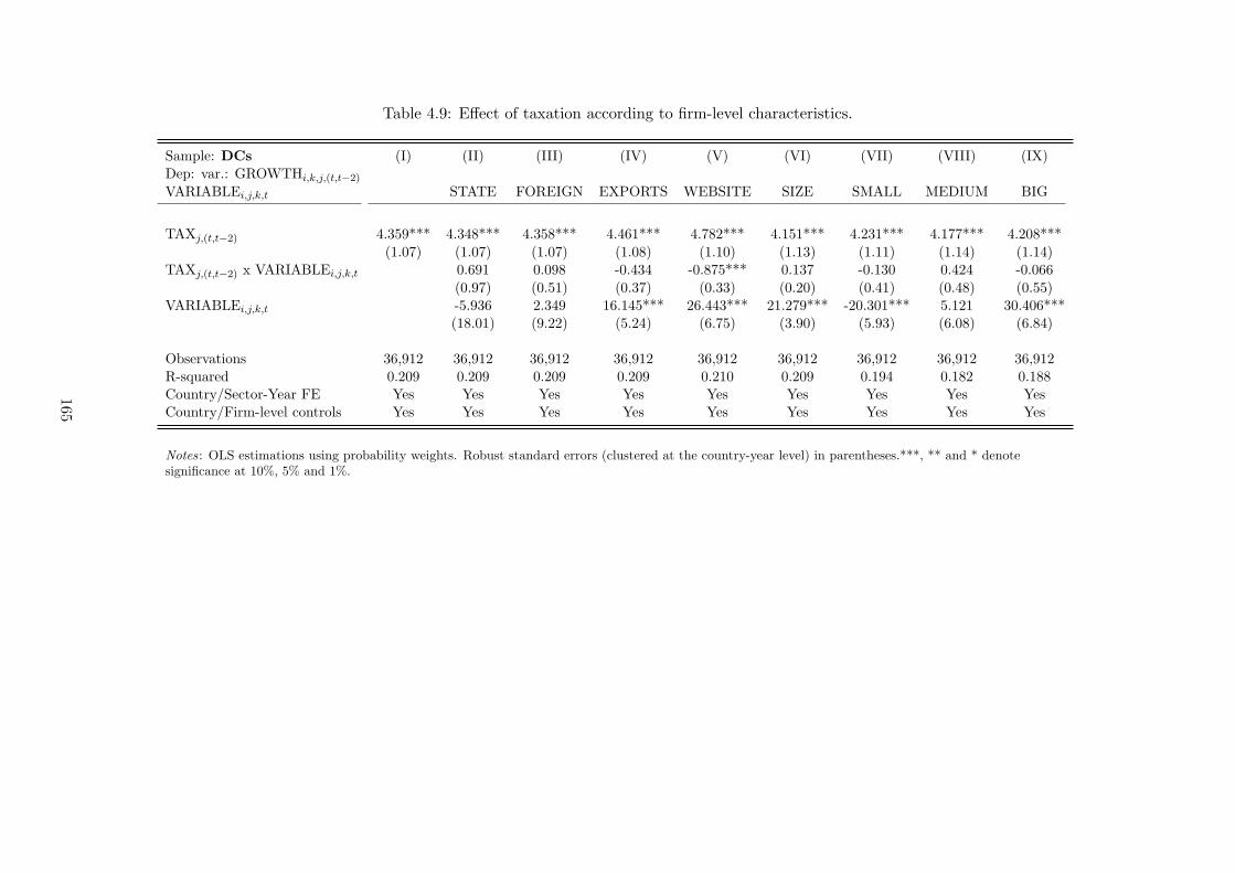
Table 4.9: Effect of taxation according to firm-level characteristics.

Sample: DCs (I) (II) (III) (IV) (V) (VI) (VII) (VIII) (IX)Dep: var.: GROWTHi,k,j,(t,t−2)

VARIABLEi,j,k,t STATE FOREIGN EXPORTS WEBSITE SIZE SMALL MEDIUM BIG

TAXj,(t,t−2) 4.359*** 4.348*** 4.358*** 4.461*** 4.782*** 4.151*** 4.231*** 4.177*** 4.208***

(1.07) (1.07) (1.07) (1.08) (1.10) (1.13) (1.11) (1.14) (1.14)TAXj,(t,t−2) x VARIABLEi,j,k,t 0.691 0.098 -0.434 -0.875*** 0.137 -0.130 0.424 -0.066

(0.97) (0.51) (0.37) (0.33) (0.20) (0.41) (0.48) (0.55)VARIABLEi,j,k,t -5.936 2.349 16.145*** 26.443*** 21.279*** -20.301*** 5.121 30.406***

(18.01) (9.22) (5.24) (6.75) (3.90) (5.93) (6.08) (6.84)

Observations 36,912 36,912 36,912 36,912 36,912 36,912 36,912 36,912 36,912R-squared 0.209 0.209 0.209 0.209 0.210 0.209 0.194 0.182 0.188Country/Sector-Year FE Yes Yes Yes Yes Yes Yes Yes Yes YesCountry/Firm-level controls Yes Yes Yes Yes Yes Yes Yes Yes Yes

Notes: OLS estimations using probability weights. Robust standard errors (clustered at the country-year level) in parentheses.***, ** and * denotesignificance at 10%, 5% and 1%.

165

Figure 4.2: Infrastructures provision and level of taxation.

Notes: Obstacle perception and taxes excluding social contribution are averaged over the period on which salesgrowth is computed (t, t-2).

We also examine whether there is greater consumption of the education input in some

sectors than in others. Taking the same input-output matrix, we construct, for each sector, the

intensity in education, Educationk, which is the share of education in the sum of all inputs.

Table 4.A4 in the Appendix A (p.175) displays the four intensities sector by sector. Table 4.10

shows the estimation results for Equation 4.2 with the different public good intensities.

We again identify two samples, the sample of all developing countries (Panel A) and the

sample restricted to LICs/LMICs (Panel B). Given that taxation may take some time to transform

into infrastructure, we examine both the effect of our usual variable of taxation averaged over

the period (t, t-2), TAXj,(t,t−2) and of taxation averaged over a longer period, TAXj,(t,t−5). The

166

interaction term between the two tax variables and the different intensities across the full sample

of developing countries does not produce clear results (Panel A). This is hardly surprising since

the positive effect of taxation is driven mostly by the LIC/LMIC sub-sample of countries. Indeed,

for Panel B, the interaction term between the tax variables, TAXj,(t,t−2) and TAXj,(t,t−5), and

intensity in public utilities and education are both positive and significant (though marginally).

This suggests that taxation has a positive effect on firms in sectors that tend to rely more on

public utilities. Results in column (IV) suggest that taxation is also benefiting firms which

activity is intensive in social sector services.

Hence, firms belonging to sectors more intensive in public goods such as electicity or eduction

tend to benefit more from taxation. In Table 4.A5 in Appendix A (p.176), we show that the

conclusions are similar when firm performance is measured with labor productivity growth

instead of sales growth.

167

Table 4.10: Channel of public good provision.

(I) (II) (III) (IV)

Dep. var.: GROWTHi,k,j,(t,t−2)

INTENSITY Pub Utilities Transport Transp Constr. Education

Panel A All DCs

with TAXj,(t,t−2)

TAX * INTENSITYk,j,(t,t−2) 14.816 9.263 9.088* 20.620

(9.44) (5.50) (5.12) (12.14)Observations 36,912 36,912 36,912 36,912R-squared 0.202 0.202 0.202 0.202No. of countries 48 48 48 48

with TAXj,(t,t−5)

TAX * INTENSITYk,j,(t,t−2) 12.289 8.714 8.401* 21.350*

(8.52) (5.05) (4.74) (12.36)Observations 36,912 36,912 36,912 36,912R-squared 0.202 0.202 0.202 0.202No. of countries 48 48 48 48

Panel B LICs/LMICs

with TAXj,(t,t−2)

TAX * INTENSITYk,j,(t,t−2) 33.188* 4.439 5.605 36.521*

(17.74) (9.50) (8.96) (17.63)Observations 21,349 21,349 21,349 21,349R-squared 0.200 0.198 0.198 0.198No. of countries 30 30 30 30

with TAXj,(t,t−5)

TAX * INTENSITYk,j,(t,t−2) 32.830* 5.485 6.641 39.776**

(17.64) (9.54) (9.03) (16.15)Observations 21,349 21,349 21,349 21,349R-squared 0.199 0.198 0.198 0.198No. of countries 30 30 30 30

Firm-level var. Yes Yes Yes YesCountry-Year FE Yes Yes Yes YesSector FE Yes Yes Yes Yes

Notes: The higher one percent of firms with the largest growth rates has been dropped from thesample. OLS estimations using firm probability weights. Robust standard-errors clustered at thesector level in parentheses. ***, ** and * denote significance at 10%, 5% and 1%.

168

4.6 Conclusion

In recent years, taxation issues have come back to center stage with a peak in interest at

the latest International Conference on Financing for Development. The public finance crisis in

advanced economies and the prioritization of national defense expenditures in response to the

terrorism threat are cutting back official development assistance budgets, and push developing

countries to look for new sources of financing (such as international financial markets for some of

them). However, even though a positive view can be taken of such options, development players

all agree that the best source of financing is inevitably domestic revenue mobilization.

The macroeconomic literature has indeed pointed up, quite extensively, the positive impact

that taxation can have on economic development. However, little work has been done on the

micro effects of domestic revenue mobilization in developing countries. The lack of contributions

on this issue is due mainly to the poor quality of taxation data available to researchers in past

decades. However, the impressive work done by the ICTD in recent years has resulted in a

priceless database (The Government Revenue Dataset) including domestic revenue time series

for more than 200 countries with high levels of disaggregation. By combining this database with

the World Bank Enterprise Surveys which contain remarkable information on firm performance

for more than 100 countries, we can now investigate the relationship between taxation and firm

performance.

Our results suggest that tax revenue benefits to firm growth in developing economies, and

especially in LICs and LMICs. This study runs several robustness checks to show that our

findings are robust to the addition of macro and firm-level covariates, and that sample dependence

does not plague our results. Throughout this paper, we also seek to identify the channels through

which taxation can positively affect firm growth. First, we find that when tax revenue is not

raised from the general public’s income or corporate profits, such as windfall revenue from natural

resources exploitation, the positive effect of taxation on firm activity disappears. We argue

that, since this kind of revenue is not levied on taxpayers, governments feel less accountable to

redistribute taxes through the provision of public goods. Then, using an alternative specification,

we provide evidence that the positive effect of domestic revenue mobilization on firm performance

is likely to be reduced when corruption is too pervasive. In particular, our results show that

this crowding-out effect of corruption is only observed for countries where tax revenue is low

and where corruption incidence is higher than in other developing countries. This suggests that

when corruption is pervasive, tax revenue is diverted and therefore not used to finance public

infrastructure vital for firm activity. In keeping with Rajan and Zingales (1998), we lastly test

whether the positive contribution of taxation to firm growth is driven by this “infrastructure

provision” argument. Using exogenous measure of infrastructure dependence, we find fragile

evidence that tax revenue has a positive effect on firms operating in sectors that tend to rely

more on public utilities, transport and education. This highlights public infrastructure as a

plausible transmission channel for the positive effect of taxation.

This study thus shows that taxation can be good for economic development, particularly for

the private sector, thus supporting improvements in domestic revenue mobilization in developing

countries. Yet our findings also underline the need for a healthy and accountable institutional

environment to turn tax revenues into growth-enhancing public goods.

169

Complementary results

Appendix A. Additional core results.

Figure 4.A1: Infrastructures provision and level of development.

Notes: For the measure of infrastructure quality, we use the perception of electricity and transport as an obstacle.Both variables are reported at the firm level within the World Bank Enterprise Survey (WBES) . We thusaggregate the measure at the country level in order to plot it with respect to the level of GDP per capita. We usefirm probability weights provided by the WBES to compute the mean value of the perception of electricity andtransport as an obstacle (0=low, 4=high) at the country-level. A higher infrastructure variable value thus denotesa stronger obstacle to firm activity.

170

Figure 4.A2: Corruption and tax revenue by income group.

Notes: Red lines represent the average value of both taxes and corruption for the entire sample of developingcountries. Numbers in each corner of the diagram report the number of LICs/LMICs and UMICs in each cardinalsquare (North-West, North-East, South-West, South-East).

171

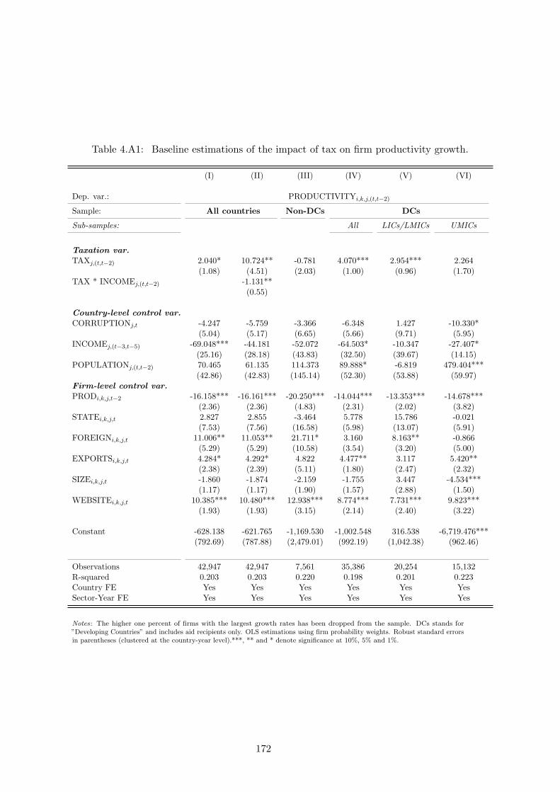
Table 4.A1: Baseline estimations of the impact of tax on firm productivity growth.

(I) (II) (III) (IV) (V) (VI)

Dep. var.: PRODUCTIVITYi,k,j,(t,t−2)

Sample: All countries Non-DCs DCs

Sub-samples: All LICs/LMICs UMICs

Taxation var.TAXj,(t,t−2) 2.040* 10.724** -0.781 4.070*** 2.954*** 2.264

(1.08) (4.51) (2.03) (1.00) (0.96) (1.70)TAX * INCOMEj,(t,t−2) -1.131**

(0.55)

Country-level control var.CORRUPTIONj,t -4.247 -5.759 -3.366 -6.348 1.427 -10.330*

(5.04) (5.17) (6.65) (5.66) (9.71) (5.95)INCOMEj,(t−3,t−5) -69.048*** -44.181 -52.072 -64.503* -10.347 -27.407*

(25.16) (28.18) (43.83) (32.50) (39.67) (14.15)POPULATIONj,(t,t−2) 70.465 61.135 114.373 89.888* -6.819 479.404***

(42.86) (42.83) (145.14) (52.30) (53.88) (59.97)Firm-level control var.PRODi,k,j,t−2 -16.158*** -16.161*** -20.250*** -14.044*** -13.353*** -14.678***

(2.36) (2.36) (4.83) (2.31) (2.02) (3.82)STATEi,k,j,t 2.827 2.855 -3.464 5.778 15.786 -0.021

(7.53) (7.56) (16.58) (5.98) (13.07) (5.91)FOREIGNi,k,j,t 11.006** 11.053** 21.711* 3.160 8.163** -0.866

(5.29) (5.29) (10.58) (3.54) (3.20) (5.00)EXPORTSi,k,j,t 4.284* 4.292* 4.822 4.477** 3.117 5.420**

(2.38) (2.39) (5.11) (1.80) (2.47) (2.32)SIZEi,k,j,t -1.860 -1.874 -2.159 -1.755 3.447 -4.534***

(1.17) (1.17) (1.90) (1.57) (2.88) (1.50)WEBSITEi,k,j,t 10.385*** 10.480*** 12.938*** 8.774*** 7.731*** 9.823***

(1.93) (1.93) (3.15) (2.14) (2.40) (3.22)

Constant -628.138 -621.765 -1,169.530 -1,002.548 316.538 -6,719.476***(792.69) (787.88) (2,479.01) (992.19) (1,042.38) (962.46)

Observations 42,947 42,947 7,561 35,386 20,254 15,132R-squared 0.203 0.203 0.220 0.198 0.201 0.223Country FE Yes Yes Yes Yes Yes YesSector-Year FE Yes Yes Yes Yes Yes Yes

Notes: The higher one percent of firms with the largest growth rates has been dropped from the sample. DCs stands for”Developing Countries” and includes aid recipients only. OLS estimations using firm probability weights. Robust standard errorsin parentheses (clustered at the country-year level).***, ** and * denote significance at 10%, 5% and 1%.

172

Table 4.A2: Additional firm covariates and TSLS estimations.

Sample: DCs (I) (II) (III) (IV) (V) (VI)Dep.: GROWTHi,k,j,(t,t−2)

VARIABLES FEMALE ELECTRY. TRANSPT. OUTAGE CELL

Panel A OLS

TAXj,(t,t−2) 4.359*** 5.456*** 4.296*** 3.980*** 4.361*** 4.061***

(1.07) (0.90) (1.09) (1.08) (1.08) (1.14)VARIABLEj,(t,t−2) -1.989 1.393 0.785 -1.663

(2.66) (1.26) (0.74) (1.66)SALEScell,j,t−2 -13.658***

(2.10)STATEcell,j,t 3.962

(12.95)FOREIGNcell,j,t 3.738

(5.76)EXPORTcell,j,t 10.579

(6.44)SIZEcell,j,t 24.211***

(4.69)WEBSITEcell,j,t 2.663

(4.76)

Panel B TSLS

TAXj,(t,t−2) 6.624** 8.108** 6.362* 5.256* 6.674** 5.042

(3.29) (3.33) (3.30) (3.17) (3.29) (3.17)VARIABLEj,(t,t−2) -1.960 1.380 0.793 -1.530

(2.63) (1.25) (0.74) (1.63)

First-step

TAX NEIGHBj,(t,t−2) 0.303*** 0.312*** 0.303*** 0.302*** 0.301*** 0.301***

(0.09) (0.09) (0.09) (0.09) (0.09) (0.09)NRR NEIGHBj,(t,t−2) -0.164** -0.167** -0.164** -0.166** -0.165** -0.166**

(0.06) (0.06) (0.06) (0.06) (0.06) (0.06)

F-Stat 1st Step (p-value) 0.000 0.000 0.000 0.000 0.000 0.000Kleibergen-Paap Wald F-Stat 14.52 13.60 14.52 14.66 14.56 14.61% bias included ≤ 15% ≤ 15% ≤ 15% ≤ 15% ≤ 15% ≤ 15%Hansen J-Stat (p-val.) 0.548 0.553 0.566 0.389 0.530 0.397Hausman endog. (p-val.) 0.501 0.392 0.544 0.794 0.495 0.770

Observations 36,912 36,004 36,812 36,567 36,695 36,912No. of countries 48 48 48 48 48 48Country FE Yes Yes Yes Yes Yes YesSector-Year FE Yes Yes Yes Yes Yes Yes

Notes: The higher one percent of firms with the largest growth rates has been dropped from the sample. PanelA: OLS estimations using probability weights. Panel B: 2SLS estimations using firm probability weights. Robuststandard errors (clustered at the country-year level) in parentheses.***, ** and * denote significance at 10%, 5%and 1%. P-value of the 2SLS coefficient for TAX in columns (VI) is 0.111.

173

Table 4.A3: Firm fixed effect estimations.

Sample: DCs (I) (II) (III) (IV)

Dep. var.: GROWTHi,k,j,(t,t−2) PRODUCTIVITYi,k,j,(t,t−2)

TAXj,(t,t−2) -2.219 38.697** -4.177* 47.754***(2.472) (14.916) (2.308) (16.108)

TAX * INCOMEj,(t−3,t−5) -5.442** -6.854***(2.094) (2.199)

CORRUPTIONj,t 8.900 12.113 25.691* 47.378***(8.795) (9.679) (13.161) (14.952)

INCOMEj,(t−3,t−5) 49.826 214.913** 91.055 317.077**(81.028) (104.764) (73.113) (114.922)

POPULATIONj,(t,t−2) 237.479** 225.993** 273.794** 154.830(104.835) (87.254) (133.052) (126.218)

SALESi,k,j,t−2 -9.709*** -10.301***(1.963) (1.925)

PRODUCTIVITYi,k,j,t−2 -11.455*** -12.430***(2.292) (2.410)

STATEi,k,j,t 15.837 15.913 24.267 23.602(12.173) (11.249) (16.378) (14.727)

FOREIGNi,k,j,t 1.044 1.896 0.076 1.113(2.005) (1.915) (2.380) (2.175)

EXPORTi,k,j,t 3.919* 4.416* -0.191 0.605(2.243) (2.168) (1.879) (1.615)

SIZEi,k,j,t 5.116** 5.714*** -4.950 -4.729(1.897) (1.752) (3.043) (3.007)

Constant -4274.364** -5306.065*** -5128.186** -4924.123**(2026.991) (1837.126) (2311.020) (2090.324)

Observations 8684 8684 7594 7594R-squared 0.211 0.224 0.186 0.198No. of countries 29 29 29 29No. of country-year obs. 58 58 58 58Firm FE Yes Yes Yes YesSector-Year FE Yes Yes Yes Yes

Notes: The higher one percent of firms with the largest growth rates has been dropped fromthe sample. DCs stands for ”Developing Countries” and includes aid recipients only. OLSestimations using firm probability weights. Robust standard errors in parentheses (clusteredat the country-year level).***, ** and * denote significance at 10%, 5% and 1%.

174

Table 4.A4: Intensities by sectors.

INTENSITY Pub Utilities Transport Transp Constr Education

MANUFACTURINGFOOD AND TOBACCO 2.535 4.668 5.046 0.001TEXTILE AND GARMENTS 2.978 3.070 3.391 0.001LEATHER 1.819 3.195 3.450 0.002WOOD AND FURNITURE 3.543 5.134 5.866 0.001PAPER AND PUBLISHING 3.664 4.876 5.494 0.063CHEMICALS 4.282 3.392 3.965 0.005RUBBER & PLASTIC 4.142 3.066 3.737 0.004METALLIC & MINER. 7.922 9.970 11.05 0.002FABRICATED METAL 4.779 3.806 4.575 0.002MACHINERY AND EQUIP. 1.539 2.492 2.887 0.003ELECTRONICS 1.729 1.666 2.150 0.005MOTOR VEHICLES 0.980 2.048 2.245 0.002REFINED PETRO 1.310 3.214 3.386 0.011OTHER MANUF 1.899 3.950 4.445 0.002

SERVICESRETAIL 5.152 7.215 8.060 1.281WHOLESALES 2.505 9.300 9.745 0.458IT 1.771 2.105 4.192 0.140TRANSPORT & CONSTR. 1.034 8.410 8.878 0.034SALES OF MOTOR VEHICLES 2.011 3.031 3.348 0.024HOTEL 6.086 3.991 4.839 0.001OTHER SERVICES 3.668 2.608 3.140 0.145

Notes: Authors’ computation.

175

Table 4.A5: Channel of public good provision.

(I) (II) (III) (IV)

Dep. var.: PRODUCTIVITYi,k,j,(t,t−2)

INTENSITY Pub Utilities Transport Transp Constr. Education

Panel A All DCs

with TAXj,(t,t−2)

TAX * INTENSITYk,j,(t,t−2) 12.553 2.887 2.457 11.593(9.04) (4.85) (4.40) (9.58)

Observations 35,386 35,386 35,386 35,386R-squared 0.194 0.193 0.193 0.194No. of countries 48 48 48 48

with TAXj,(t,t−5)

TAX * INTENSITYk,j,(t,t−2) 11.004 1.691 1.191 11.507(8.54) (4.55) (4.14) (10.38)

Observations 35,386 35,386 35,386 35,386R-squared 0.194 0.193 0.193 0.194No. of countries 48 48 48 48

Panel B LICs/LMICs

with TAXj,(t,t−2)

TAX * INTENSITYk,j,(t,t−2) 26.764* 4.944 5.246 22.603*(14.41) (7.48) (6.89) (11.74)

Observations 20,254 20,254 20,254 20,254R-squared 0.192 0.191 0.191 0.191No. of countries 30 30 30 30

with TAXj,(t,t−5)

TAX * INTENSITYk,j,(t,t−2) 27.155* 5.191 5.513 25.751*(14.33) (7.46) (6.89) (11.02)

Observations 20,254 20,254 20,254 20,254R-squared 0.192 0.191 0.191 0.191No. of countries 30 30 30 30

Firm-level var. Yes Yes Yes YesCountry-Year FE Yes Yes Yes YesSector FE Yes Yes Yes Yes

Notes: The higher one percent of firms with the largest growth rates has been dropped from thesample. OLS estimations using firm probability weights. Robust standard-errors clustered at thesector level in parentheses. ***, ** and * denote significance at 10%, 5% and 1%.

176

Appendix B. Sample discussion and composition.

Discussion about sample restrictions:

As exposed by equation 4.1 in the section 4.2, our empirical specification includes country-

fixed effects and thus aims at investigating the effects of changes in tax revenue from the

country-average level of tax revenue on the deviation of a given firm performance from the

country-average’s firm performance. Our model hence captures the effect of tax revenue changes

on the within variation of firm growth. Omitting the set of control variables in order to simplify

the writings and using the WITHIN transformation, the empirical specification can be written

as follows:

GROWTHi,k,j,(t,t−2) −GROWTH•,•,j,• = α+ β[

TAXj,(t,t−2) − TAXj,•

]

+ τk,t + εi,k,j,t (4.3)

Looking at this equation, it appears as quite obvious that including countries with only one

WBES survey will not bring any information for our empirical specification. Indeed, within

regressions for countries with only one survey would lead to have TAXj,(t,t−2) = TAXj,• and thus

would artificially include zeros into the regression. Keeping these countries into the sample would

thus provide no additional information as regards the effect of tax revenue on firm performance

and would bias the interpretation of the β coefficient, since it reflects the average effect of tax

revenue on firm performance, not for the entire sample, but only for countries where two surveys

are available. We therefore decide to exclude countries with one WBES survey from the sample

of study. Table 4.B1 (below) presents the final sample considered for this study.

177

Table 4.B1: Sample of study.

country nb. of firms year of survey country nb. of firms year of survey

Afghanistan 332 2008; 2014 Lithuania 374 2009; 2013Albania 260 2007; 2013 Macedonia, FYR 583 2009; 2013Argentina 1,574 2006; 2010 Malawi 397 2009; 2014Armenia 394 2009; 2013 Mali 502 2007; 2010Azerbaijan 460 2009; 2013 Mexico 2,349 2006; 2010Bangladesh 2,761 2007; 2013 Moldova 586 2009; 2013Belarus 384 2008; 2013 Mongolia 622 2009; 2013Bhutan 444 2009; 2015 Montenegro 162 2009; 2013Bolivia 533 2006; 2010 Namibia 428 2006; 2014Bosnia and Herzegovina 517 2009; 2013 Nepal 772 2009; 2013Botswana 444 2006; 2010 Nicaragua 635 2006; 2010Bulgaria 1,343 2007; 2009; 2013 Pakistan 1,253 2007; 2013Burundi 351 2006; 2014 Panama 468 2006; 2010Chile 1,596 2006; 2010 Paraguay 592 2006; 2010Colombia 1,613 2006; 2010 Peru 1,36 2006; 2010Congo, Dem. Rep. 826 2006; 2010; 2013 Poland 561 2009; 2013Croatia 766 2007; 2013 Romania 678 2009; 2013Czech Republic 357 2009; 2013 Russian Federation 2,922 2009; 2012Ecuador 738 2006; 2010 Rwanda 318 2006; 2011El Salvador 781 2006; 2010 Senegal 759 2007; 2014Georgia 401 2008; 2013 Serbia 598 2009; 2013Ghana 900 2007; 2013 Tajikistan 386 2008; 2013Guatemala 813 2006; 2010 Tanzania 716 2006; 2013Honduras 564 2006; 2010 Turkey 1,256 2008; 2013Hungary 402 2009; 2013 Uganda 900 2006; 2013Kenya 1,184 2007; 2013 Ukraine 824 2008; 2013Kyrgyz Republic 346 2009; 2013 Uruguay 773 2006; 2010Lao PDR 526 2008; 2012 Zambia 931 2007; 2013Latvia 388 2009; 2013

Notes: Countries in italic and bold font are not classified as developing countries.

178

Appendix C. Computation method for average idiosyncratic shocks of largest firms.

In keeping with Gabaix (2011), we start by identifying the largest firms for each developing

country of the sample. We thus first select the top 5% firms of each country (and for each year

of the country-survey) with respect to the level of their sales in t-3. This leads us to consider a

sample of 1,698 firms across 48 developing countries.

We then run productivity growth estimates on this restricted subsample of M large firms (so

at the firm-level), where the within-country variation in productivity growth is explained by

various firm-level controls such as the productivity in t− 2, a dummy variable denoting whether

the firm is partly state-owned, foreign-owned, has some exporting activities, or has a website. In

addition to the country-fixed effects, we also augment the specification with time-fixed effects.

We thus assume that productivity evolves as:

PRODUCTIV ITYi,k,j,(t,t−2) = βXi,k,j,t + µj + δt + ǫi,k,j,t (4.4)

where Xi,k,j,t includes the above defined firm level controls. As in Gabaix (2011), we investigate

whether ǫi,k,j,t, which denotes idiosyncratic component of total factor productivity growth of

large firms, can affect aggregate economic developments. Using predicted residuals from equation

4.4, we compute the sum of idiosyncratic firm shocks, weighted by size, which thus represents

the “granular residual” (Γ) and is obtained as follows:

Γj,t =M∑

i=1

SALESi,k,j,t−2

SALESj,t−2× ǫi,k,j,t (4.5)

where SALESj,t−2 denotes the country-level amount of sales (in constant USD) in t − 2 for

country j, and SALESi,k,j,t−2, the firm-level amount of sales (in constant USD) in t − 2 for

the large firm i, in sector k, in country j. Lastly, ǫi,k,j,t represents the predicted idiosyncratic

component of total factor productivity growth for the large firm i, in sector k, in country j at

year t derived from equation 4.4.

We also defined two alternative measures of Γj,t by changing specification 4.4. We first

replace µj with µk,j in order to observe the within-country-sector variation of productivity growth.

Γ bisj,t is thus obtained using the predicted residuals stemming from this new specification.

Lastly, as in Gabaix (2011), we compute Γ sectj,t which uses predicted residuals derived from

the equation 4.4, where we only consider as explanatory variable country-sector-year fixed effects,

and thus leads to obtain predicted residuals which represent the difference in productivity growth

for large firms as compared with the average growth rate of large firms in sector k, country j, in

year t. Note that we also compute these three variables when considering the 10% largest firms‘,

instead of the top 5%.

We then use these various measures of “granular residual” to explain aggregate economic

developments (see Table 4.3 in the core text).

179

Appendix D. Additional Robustness checks.

Table 4.D1: Estimations with alternative fixed effects specifications and clusters.

(I) (II) (III) (IV) (V) (VI)

Dep. var. GROWTHi,k,j,(t,t−2)

Sample All countries Non-DCs DCs

Sub-samples All LICs/LMICs UMICs

Panel A (country, sector, year fixed effects - cluster (country-year level)

TAXj,(t,t−2) 1.782 17.142*** -3.086** 4.777*** 3.751*** 1.526(1.13) (5.06) (1.40) (1.06) (1.34) (2.33)

TAX * INCOMEj,(t,t−2) -2.005***(0.62)

Panel B (country, sector-year fixed effects - cluster (country level)

TAXj,(t,t−2) 1.327 14.414*** -3.064* 4.359*** 3.238* 2.164(1.43) (5.17) (1.48) (1.36) (1.79) (2.92)

TAX * INCOMEj,(t,t−2) -1.706***(0.63)

Panel C (country, sector, year fixed effects - cluster (country level)

TAXj,(t,t−2) 1.782 17.142*** -3.086* 4.777*** 3.751** 1.526(1.46) (5.06) (1.54) (1.35) (1.67) (3.21)

TAX * INCOMEj,(t,t−2) -2.005***(0.62)

Observations 44,703 44,703 7,791 36,912 21,349 15,563No. of countries 57 57 9 48 30 18No. of country-level obs. 116 116 19 97 61 36

Notes: The higher one percent of firms with the largest growth rates has been dropped from the sample.OLS estimations using firm probability weights. Robust standard-errors in parentheses (clustered at thelevel specified for each panel). ***, ** and * denote significance at 10%, 5% and 1%.

180

Table 4.D2: Estimations on regional sub-samples.

Sample: DCs (I) (II) (III) (IV) (V) (VI)

Dep. var.: GROWTHi,k,j,(t,t−2)

Region dropped: none EAP ECA LAC SA SSA

TAXj,(t,t−2) 4.359*** 4.792*** 6.034*** 3.195** 3.674*** 4.732***(1.07) (1.05) (1.41) (1.38) (1.33) (1.10)

Impact tax (+10%) 46.01 50.48 68.37 36.11 37.64 46.32

Observations 36,912 35,764 29,755 22,523 31,350 28,256R-squared 0.209 0.210 0.179 0.233 0.211 0.220Nb. of countries 48 46 34 34 43 35Countries dropped 2 14 14 5 13Country-level var. Yes Yes Yes Yes YesFirm-level var. Yes Yes Yes Yes YesCountry FE Yes Yes Yes Yes YesSector-Year FE Yes Yes Yes Yes Yes

Notes: The higher one percent of firms with the largest growth rates has been droppedfrom the sample. EAP stands for East-Asia and Pacific, ECA for Europe and CentralAsia, LAC for Latin America and Caribbean, SA for South-Asia, and finally SSA forSub-Saharan Africa. OLS estimations using firm probability weights. Robust standard-errors clustered at the country-year level in parentheses. ***, ** and * denote significanceat 10%, 5% and 1%.

181

Table 4.D3: Dropping one country at a time.

Sample: DCs (I) (II) (III) (IV) (V) (VI) (VII)

Dep. var.: GROWTHi,k,j,(t,t−2)

Country omitted AFG ALB ARG ARM AZE BGD

TAXj,(t,t−2) 4.359*** 4.598*** 4.364*** 4.306*** 4.585*** 4.607*** 3.492***(1.07) (1.07) (1.07) (1.07) (1.07) (1.04) (1.10)

Observations 36,912 36,580 36,652 35,338 36,518 36,452 34,151

Country omitted BLR BTN BOL BIH BWA BDI CHL

TAXj,(t,t−2) 3.399*** 4.357*** 3.716*** 4.744*** 4.320*** 4.674*** 4.292***(1.17) (1.07) (1.18) (1.03) (1.07) (1.08) (1.08)

Observations 36,528 36,468 36,379 36,395 36,468 36,561 35,316

Country omitted COL ZAR ECU SLV GEO GHA GTM

TAXj,(t,t−2) 4.356*** 4.733*** 4.238*** 4.301*** 3.692*** 4.088*** 4.460***(1.07) (1.01) (1.09) (1.08) (1.09) (1.06) (1.16)

Observations 35,299 36,086 36,174 36,131 36,511 36,012 36,099

Country omitted HND KEN KGZ LAO MKD MWI MLI

TAXj,(t,t−2) 4.463*** 4.293*** 4.342*** 4.373*** 4.422*** 4.949*** 4.500***(1.08) (1.04) (1.07) (1.07) (1.07) (0.99) (1.07)

Observations 36,348 35,728 36,566 36,386 36,329 36,515 36,410

Country omitted MEX MDA MNG MNE NAM NPL NIC

TAXj,(t,t−2) 4.272*** 4.682*** 4.776*** 4.443*** 4.070*** 4.444*** 4.463***(1.10) (1.11) (1.05) (1.09) (1.32) (1.25) (1.05)

Observations 34,563 36,326 36,290 36,750 36,484 36,140 36,277

Country omitted PAK PAN PRY PER RWA SEN SRB

TAXj,(t,t−2) 4.414*** 4.324*** 4.322*** 4.070*** 4.360*** 4.538*** 4.172***(1.08) (1.08) (1.08) (1.14) (1.07) (1.11) (1.08)

Observations 35,659 36,444 36,320 35,552 36,594 36,153 36,314

Country omitted TJK TZA TUR UGA UKR URY ZMB

TAXj,(t,t−2) 4.388*** 4.414*** 4.143*** 4.298*** 4.258*** 4.261*** 4.347***(1.07) (1.07) (1.20) (1.08) (1.04) (1.09) (1.09)

Observations 36,526 36,196 35,656 36,012 36,088 36,139 35,981

Notes: The higher one percent of firms with the largest growth rates has been dropped from the sample.OLS estimations using firm probability weights. Robust standard-errors clustered at the country-year levelin parentheses. ***, ** and * denote significance at 10%, 5% and 1%.

182

Table 4.D4: Dropping one sector at a time.

Sample: DCs (I) (II) (III)

Dep. var.: GROWTHi,k,j,(t,t−2)

Omitted sector: Food & Tobacco Textile & Garments Leather

TAXj,(t,t−2) 4.339*** 4.429*** 4.291***(1.13) (1.07) (1.07)

Observations 31,831 31,881 36,235

Omitted sector: Wood & Furnitures Paper & Publishing Refined petroleum

TAXj,(t,t−2) 4.512*** 4.246*** 4.363***(1.17) (1.05) (1.07)

Observations 35,073 35,875 36,880

Omitted sector: Chemicals Rubber & Plastics Metal. & non-Met. Mineral

TAXj,(t,t−2) 4.582*** 4.452*** 3.948***(1.06) (1.07) (1.00)

Observations 34,686 35,876 35,287

Omitted sector: Fabricated Metal pdt Machinery & Equipment Electronics

TAXj,(t,t−2) 4.158*** 4.372*** 4.352***(1.06) (1.08) (1.08)

Observations 35,141 35,911 36,430

Omitted sector: Motor Vehicles Other Manufacturing Sales of Motor Vehicles

TAXj,(t,t−2) 4.348*** 4.313*** 4.537***(1.07) (1.10) (1.09)

Observations 36,695 36,468 36,166

Omitted sector: Wholesales trade Retail trade Hotel & Restaurants

TAXj,(t,t−2) 4.636*** 4.408*** 4.662***(1.17) (1.18) (1.03)

Observations 32,600 35,389 35,432

Omitted sector: IT Transport & Constr. Other services

TAXj,(t,t−2) 4.519*** 3.571*** 4.428***(1.12) (1.06) (1.22)

Observations 36,511 34,250 33,623

Notes: The higher one percent of firms with the largest growth rates has been dropped from the sample.OLS estimations using firm probability weights. Robust standard-errors clustered at the country-year levelin parentheses. ***, ** and * denote significance at 10%, 5% and 1%.

183

Table 4.D5: Sensitivity to firms’ characteristics.

Effect of TAXj,(t,t−2) on GROWTHi,k,j,(t,t−2)

Panel A: All firms 4.359*** (1.07)Observations 36,912

Panel B: Not owned by the state 4.314*** (1.06)Observations 36,394

Panel C: Not foreign-owned 4.270*** (1.07)Observations 32,885

Panel D: Exporting firms 5.465** (2.09)Observations 9,286

Panel E: Not exporting firms 4.211*** (1.13)Observations 27,626

Panel F: More than 20 employees 2.800** (1.32)Observations 20,056

Panel G: Not medium firms (20-100 employees) 5.449*** (1.51)Observations 24,729

Panel H: Less than 100 employees 4.272*** (1.15)Observations 29,941

Panel J: Without a website 5.555*** (1.56)Observations 20,968

Panel I: With a website 3.518** (1.34)Observations 15,944

Notes: The higher one percent of firms with the largest growth rates hasbeen dropped from the sample. OLS estimations using firm probabilityweights. Robust standard-errors clustered at the country-year level inparentheses. ***, ** and * denote significance at 10%, 5% and 1%.

184

Table 4.D6: Random draw of firms.

Dep. var.: GROWTHi,k,j,(t,t−2) (1) (2) (3)No. of firms randomly draw 100 200 300

Coefficient of TAXj,(t,t−2), 500 replicationsMean 2.968 3.345 3.391Standard deviation 1.442 0.609 0.414Percent not significant 30.6 1.8 0

Observations 9,613 18,153 24,338Country FE Yes Yes YesSector-Year FE Yes Yes YesLevel of se clustering country-year country-year country-yearFirm-level controls Yes Yes YesCountry-level controls Yes Yes Yes

185

General conclusion

Since July 2015, the Addis Ababa Action Agenda strongly emphasizes the need for developing

countries to increase financial resources in order to face upcoming challenges resulting from

global warming and to lift the bottom billion out of the poverty. Among the numerous solutions

that the AAAA suggests to satisfy such financial needs, taxation has been appointed as a top

priority. Historically, and in spite of all the efforts deployed by national governments and the

international community, domestic revenue mobilization in developing countries has encountered

many obstacles hindering its development. Fortunately, over the last few years, and after

decades of stagnation, taxation started to improve, hence highlighting the willigness of policy

makers in developing countries to be the primary actors of their country’s developement as

well as their increasing awareness about the need to develop solid and efficient tax systems.

However, although having a crucial role in the achievement of the SGDs, the AAAA has pointed

out that taxation should be considered as a necessary but not sufficient condition. Indeed,

as stated by Maria Emma Meija Velez (President of ECOSOC) “the importance of domestic

resources mobilization cannot be overemphasized. But, that cannot happen without an enabling

international environment in support of development”.16 The AAAA thus underlines the need

for developing countries to resort to other financial sources such as foreign investment, trade,

international aid, and both domestic and external borrowing. However, such strategy will help

countries reaching these goals only if increasing resort to external financing and borrowing is

associated with sound economic management and do not lead to the same debt issues than those

experienced throughout the 1980s and 1990s.

Consequently, alongside these recommendations, the AAAA restated the need to secure

LICs’ long term debt sustainability, through debt restructuring and for the most extreme cases,

debt relief. Yet, although the multilateral debt relief initiatives of the early 2000s undoubtedly

succeeded in reducing debt burden, the academic literature has provided very few empirical

evidence about the economic effects of these policies and their impacts on the overall economic

development.

This thesis first proposes an empirical assessment of the debt relief effects on public finance

in recipient countries, focusing both on the resource and spending sides. Reviewing the largest

debt relief programs for LICs of the past decades, the first three essays highlight that debt

cancellations under both the Enhanced HIPC initiative and the MDRI have significantly affected,

mostly in a positive way, public finance of beneficiary governments. Lastly, the fourth essay

revisits the growth-taxation nexus by investigating the effects on domestic revenue mobilization

16http://www.un.org/esa/ffd/ffd3/wp-content/uploads/sites/2/2015/07/Statement-by-ECOSOC.pdf

187

on private sector development in order to provide evidence that AAAA’s recommendations do

not contradict each other.

Chapter 1 exposes that debt relief granted under the Enhanced HIPC initiative have re-

sulted, mainly through the channel of conditionality, in public investment increase for beneficiary

countries. In line with the debt overhang theory, such effects seem to be higher for HIPCs which

were repaying their debt prior to debt relief. Results thus suggest that the debt relief initiatives

have helped freeing up additional resources intended to finance development infrastructures and

reduce poverty in order to reach the Millennium Development Goals, supposed to be achieved

by 2015. Moreover, our analysis also highlights that investment undertaken after the Enhanced

HIPC initiative could benefit from extra financial support thanks to ultimate debt relief granted

under the MDRI. As a result, it seems fair to say that debt relief contributes to finance the

development of LICs, and that its impact might be enhanced when debt relief comes with strong

and development-oriented conditionality. In addition, our results also support a positive contri-

bution of these initiatives on domestic revenue mobilization which, according to us, is probably

derived from the programs’ conditionality. Such increase is all the more beneficial to HIPCs

that expansion of public domestic resources might help financing upcoming spending needed to

maintain public investment undertaken thanks to these multilateral debt relief initiatives.

Yet, the relationship between taxation and debt relief is not that straightforward. Building

on first chapter’s findings and a large theoretical body investigating the relationship between

adjustment effort and debt relief, chapter 2 intends to empirically assess the effect of these

initiatives on recipient governments’ adjustment efforts, when those relate to fiscal capacity.

Results suggest that the positive contribution of debt relief to tax effort is, by large, due to the

conditionality and the efforts made beforehand in order to be eligible for the initiative. Indeed,

since one of the various requirements for benefiting from the Enhanced HIPC initiative is to

implement a macro-stabilizing program —which often aims at improving tax system functioning—

, HIPCs tend to strongly comply with conditionality by increasing their effort over the years

following first debt cancellations.

Nevertheless, additional results suggest that HIPCs ease off their tax effort once they have

been granted full and irrevocable debt relief under the MDRI, thus emphasizing moral hazard

stemming from the design of these initiative where once countries complete the debt relief process

this marks the end of the conditionality and IFIs’ monitoring. Yet, moral hazard around the

MDRI is not observed for all HIPCs and seems to be driven by some countries’ peculiarities. I

find that tax effort is more likely to reduce after MDRI when governments of recipient countries

are characterized by large instability. Political instability has indeed been shown as conducive

to behaviors which favor short term consumption instead of investment which would secure

larger revenue and increase future consumption. Under debt relief settings, this translates into a

reduction of investment in fiscal capacity once governments have obtained full debt relief and

are not subject to IFIs monitoring anymore. In the same vein, additional findings suggest that

government with weak institutions before the MDRI experience more difficulties in sustaining

tax effort levels once they have benefited from this initiative. While institutions quality partly

188

reflects government’s performance as regards taxation, one can fairly assume that, without

changing their institutional quality, countries could overperform in terms of tax effort in order

to become eligible, maintain significant adjustment efforts as long as there is debt relief to get,

and then slacken off once complete debt forgiveness is granted. In such scenario, countries with

weak institutions quality right before being granted debt relief under the MDRI are more prone

to adopt such behaviors, as our findings suggest.

Lastly, results also show that moral hazard might be fostered by the surfacing of new financ-

ing sources such as domestic debt markets. Indeed, easing-off in tax effort seems to be more

important for countries where domestic debt increases in the post-MDRI period. This might be

explained by large financing resources being easier to get with immediate borrowing (especially

when borrowing is not subject to exchange risks), rather than through improvement in tax

system which pays off later on, and for which outcomes are likely to depend on the economic

and political environment.

Chapter 3 follows chapter 2 findings but focuses the analysis on the relationship between

debt relief and external public financing. Departing from the existing literature about market

access and reputation costs derived from sovereign default, we try to empirically assess the

consequences of debt relief on borrowing to external private creditors. Simultaneously, we also

review the effect of these initiatives on lending condition from the first providers of debt relief;

the official creditors. We find that having benefited from the multilateral debt relief initiatives,

yields official creditors to tighten their lending conditions which translates into shorter grace and

maturity periods and in fine, lower grant-element on new financing. Results also suggest that

official creditors, besides increasing the cost of financing for HIPCs as compared with other LICs,

significantly reduce official aid flows. Going further, we observe that such reduction is mainly

driven by the diminution of bilateral gross aid transfers (both loans and grants) and multilateral

loans. Consequently, given the financing needs of HIPCs to achieve sustainable development (as

defined by the SDGs), and their renewed borrowing capacity, it seems that shortfall in official

flows is compensated (though not fully offset) with loans from private creditors.

The last section of our study also suggests that the interest of private creditors for HIPCs

—which were historically excluded from international financial markets—, materializes only after

the MDRI, once benefiting governments regained a full borrowing capacity. In addition, we

provide some evidence that foreign private banks are more likely to lend to HIPCs during

financial bust in advanced economies. Low market returns and sluggish economic environment

in high-income countries hence lead investors to seek for high-return investment in developing

countries, among which, HIPCs seem to be favored. As a result, though the external debt of

HIPCs was (on average) nearly null after additional cancellations under the MDRI, increasing

amounts of loans contracted from private creditors, by definition at larger costs, lays doubts

about the effects of this new type of financing on future debt sustainability.

Lastly, chapter 4 departs from debt relief to revisit the taxation-growth nexus adopting

a macro-micro approach. Using firm-level data, this last essay tries to empirically assess the

effect of taxation on firms performance in the particular context of developing countries. While

189

increase in taxation is supposed to raise up production costs and distort investment incentives,

such additional revenue can be used to finance public goods such as infrastructure which are

crucial for firms activity. Though we expect the overall effect of taxation to be negative in

advanced economies given the already satisfying stock of public infrastructures, taxation could

be beneficial in developing countries where marginal returns of public spending are substantial,

especially for private businesses. Our findings support these theoretical intuitions, highlight-

ing a positive effect of taxation on the growth rate of firms’ sales and labor productivity for

firms operating in developing countries. Yet subsequent findings suggest that such positive

effect can however be reduced when corruption is significant, in particular for LICs’ firms.

This let us think that the positive effect of taxation on firms performance goes through the

provision of public goods since when corruption is spread all over the economy and among

public institutions in particular, extra tax revenue hardly translate in additional public goods

intended to benefit to the private sector. Lastly, we investigate this public good provision channel

in a more straightforward way using an approach similar to the one of Rajan and Zingales

(1998) where we estimate the impact of taxation on firms operating in sectors structurally more

dependent in infrastructure. Results provide fragile evidence that taxation is more beneficial

for firms belonging to sectors that are more dependent on public utilities, transport and con-

struction activities, or that intensively resort to human capital, thus highlighting sound public

goods provision as a potential determinant of the effect of taxation on private sector development.

∗ ∗ ∗

These various findings line up with the recommendations made by the Addis Ababa Agenda

for Actions and suggest that its objectives do not contradict each other. Indeed, chapter 4

underlines the crucial role of taxation in private sector development. However, this essay also

underlines necessary prerequisites for such relationship to be observed and warns about the

consequences of rising domestic revenue mobilization in highly corrupt environment where a

significant share of of collected taxes would be diverted and where resulting public goods would

be not enough to offset the additional costs derived from taxation.

Among the potential ways for improving fiscal capacity in low income countries, the first

two essays shows that debt relief might be of importance in that respect. Findings highlights

a positive contribution of debt relief to tax effort in recipient countries which however does

not seem to be robust for every governments being granted debt relief. Indeed, results suggest

that governments with high preference for present and low quality institutions are more likely

to slacken off once they have benefited from ultimate debt relief and that the IFIs monitoring

stops. Moral hazard might however be overcome by reinforcing cooperation between recipi-

ent governments and IFIs. According to our results, for governments exposing peculiarities

identified as driving moral hazard around the MDRI, it would be preferable to ensure that

tax reforms and other fiscal improvements are settle and associated with sound managment

before granting ultimate debt relief in order to secure the initial efforts. This is even more

important in a context where easing off in tax effort seems to be associated with more borrow-

190

ing on domestic and international debt markets where lending conditions are less favourable

than what these countries used to get. The necessecity to secure the government fiscal capac-

ity thus appears as necessary if one wants to avoid repeating past errors that lead numerous

LICs trapped in the debt spiral and the international community to made substantial concessions.

Further research thus needs to be done as regards the financing strategies of HIPCs. Recent

evolutions fueled serious doubts regarding their capacity to embrace a virtuous way of financing

their development. These concerns have been formulated by Stiglitz and Rashid (2013) and again

by the IMF over the past few years. As stated during the Addis Ababa conference, domestic

efforts need to be done but also necessitate an enabling international environment preventing

low income countries to face debt distress again. In light of the results exposed throughout this

thesis, it would be prejudicial for countries having benefited from debt relief to go back to old

policies since sustained tax effort has been shown as conducive to economic growth and to the

private sector development in particular, which seems fundamental given the ambitious SDGs

supposed to be achieved by 2030.

191

Bibliography

Addison, T. (2008). Debt relief: The development and poverty impact. In Development Finance in theGlobal Economy, pages 216–235. Springer.

Addison, T., Mavrotas, G., and McGillivray, M. (2005). Aid, debt relief and new sources of finance formeeting the millennium development goals. Journal of International Affairs, pages 113–127.

Afonso, A. (2003). Understanding the determinants of sovereign debt ratings: Evidence for the twoleading agencies. Journal of Economics and Finance, 27(1):56–74.

Afonso, A., Gomes, P. M., and Rother, P. (2007). What ’Hides’ Behind Sovereign Debt Ratings?

Agbeyegbe, T. D., Stotsky, J., and WoldeMariam, A. (2006). Trade liberalization, exchange rate changes,and tax revenue in Sub-Saharan Africa. Journal of Asian Economics, 17(2):261–284.

Aghion, P., Akcigit, U., Cage, J., and Kerr, W. R. (2016). Taxation, corruption, and growth. EuropeanEconomic Review, 86:24–51.

Aguiar, M. and Gopinath, G. (2006). Defaultable debt, interest rates and the current account. Journal ofInternational Economics, 69(1):64–83.

Alacevich, M. and Asso, P. F. (2009). Money Doctoring after World War II: Arthur I. Bloomfield andthe Federal Reserve Missions to South Korea. History of Political Economy, 41(2):249–270.

Alesina, A. and Dollar, D. (2000). Who Gives Foreign Aid to Whom and Why? Journal of EconomicGrowth, 5(1):33–63.

Alesina, A. and Weder, B. (2002). Do Corrupt Governments Receive Less Foreign Aid? AmericanEconomic Review, 4(92):1126–1137.

Angrist, J. D. and Pischke, J.-S. (2008). Mostly harmless econometrics: An empiricist’s companion.Princeton university press.

Arellano, M. and Bond, S. (1991). Some Tests of Specification for Panel Data: Monte carlo Evidence andan Application to Employment Equations. The Review of Economic Studies, 58(2):277–297.

Arellano, M. and Bover, O. (1995). Another look at the instrumental variable estimation of error-components models. Journal of Econometrics, 68(1):29–51.

Aterido, R., Hallward-Driemeier, M., and Pages, C. (2011). Big Constraints to Small Firms’ Growth?Business Environment and Employment Growth across Firms. Economic Development and CulturalChange, 59(3):609–647.

Auerbach, A. J., Aaron, H. J., and Hall, R. E. (1983). Corporate Taxation in the United States. BrookingsPapers on Economic Activity, pages 451–513.

Bahl, R. W. (1971). A regression approach to tax effort and tax ratio analysis. Staff Papers-InternationalMonetary Fund, pages 570–612.

Baldacci, E., Gupta, S., and Mati, A. (2008). Is it (Still) Mostly Fiscal? Determinants of SovereignSpreads in Emerging Markets. IMF Working Papers, pages 1–23.

192

Barro, R. J. (1990). Government Spending in a Simple Model of Endogeneous Growth. Journal ofPolitical Economy, 98(5, Part 2):S103–S125.

Baskaran, T. and Bigsten, A. (2013). Fiscal Capacity and the Quality of Government in Sub-SaharanAfrica. World Development, 45:92–107.

Baunsgaard, T. and Keen, M. (2010). Tax revenue and (or?) trade liberalization. Journal of PublicEconomics, 94(9):563–577.

Beck, T., Clarke, G., Groff, A., Keefer, P., and Walsh, P. (2001). New Tools in Comparative PoliticalEconomy: The Database of Political Institutions. the World Bank Economic Review, 15(1):165–176.

Benczur, P. and Ilut, C. L. (2015). Evidence for relational contracts in sovereign bank lending. Journalof the European Economic Association.

Berthelemy, J.-C. (2006). Bilateral Donors’ Interest vs. Recipients’ Development Motives in Aid Allocation:Do All Donors Behave the Same? Review of Development Economics, 10(2):179–194.

Berthelemy, J.-C. and Tichit, A. (2004). Bilateral donors’ aid allocation decisions—a three-dimensionalpanel analysis. International Review of Economics & Finance, 13(3):253–274.

Besley, T. and Persson, T. (2007). The Origins of State Capacity: Property Rights, Taxation, and Politics.Technical report, National Bureau of Economic Research.

Besley, T. and Persson, T. (2010). State Capacity, Conflict, and Development. Econometrica, 78(1):1–34.

Besley, T. and Persson, T. (2014). Why Do Developing Countries Tax So Little? The Journal of EconomicPerspectives, 28(4):99–120.

Besley, T. J. and Persson, T. (2013). Taxation and Development.

Bigsten, A. and Soderbom, M. (2006). What Have We Learned from a Decade of Manufacturing EnterpriseSurveys in Africa? The World Bank Research Observer, 21(2):241–265.

Bird, G. and Rowlands, D. (2001). IMF lending: how is it affected by economic, political and institutionalfactors? The Journal of Policy Reform, 4(3):243–270.

Bird, R. M., Martinez-Vazquez, J., and Torgler, B. (2008). Tax Effort in Developing Countries and HighIncome Countries: The Impact of Corruption, Voice and Accountability. Economic Analysis and Policy,38(1):55.

Bolnick, B. R. (1978). Demographic effects on tax ratios in developing countries. Journal of DevelopmentEconomics, 5(3):283–306.

Borensztein, E. (1990). Debt overhang, credit rationing and investment. Journal of DevelopmentEconomics, 32(2):315–335.

Borensztein, E. and Panizza, U. (2009). The costs of sovereign default. IMF Economic Review, 56(4):683–741.

Bornhorst, F., Gupta, S., and Thornton, J. (2009). Natural resource endowments and the domesticrevenue effort. European Journal of Political Economy, 25(4):439–446.

Bougouin, A.-S. and Raffinot, M. (2003). The HIPC Initiative and poverty reduction. In New InternationalPoverty Reduction Strategies, pages 239–264. Routledge.

Boyce, J. K. and Ndikumana, L. (2011). Africa’s odious debts: how foreign loans and capital flight bled acontinent. Zed Books.

Burgess, R. and Stern, N. (1993). Taxation and Development. Journal of Economic Literature, pages762–830.

Cantor, R. and Packer, F. (1996). Determinants and Impact of Sovereign Credit Ratings. EconomicPolicy Review, 2(2).

193

Carroll, R., Holtz-Eakin, D., Rider, M., and Rosen, H. S. (2001). Personal Income Taxes and the Growthof Small Firms. Tax policy and the economy, 15:121–147.

Cassimon, D. and Campenhout, B. V. (2007). Aid Effectiveness, Debt Relief and Public Finance Response:Evidence from a Panel of HIPC Countries. Review of World Economics (Weltwirtschaftliches Archiv),143(4):742–763.

Cassimon, D. and Van Campenhout, B. (2008). Comparative Fiscal Response Effects of Debt Relief: AnApplication to african hipcs. South African Journal of Economics, 76(3):427–442.

Cassimon, D., Van Campenhout, B., Ferry, M., and Raffinot, M. (2015). Africa: Out of debt, into fiscalspace? Dynamic fiscal impact of the debt relief initiatives on African Heavily Indebted Poor Countries(HIPCs). International Economics, 144:29–52.

Chamley, C. (1986). Optimal Taxation of Capital Income in General Equilibrium with Infinite Lives.Econometrica: Journal of the Econometric Society, pages 607–622.

Chauvet, L. and Ehrhart, H. (2015). Aid and Growth. Evidence from Firm-Level Data. Working papers563, Banque de France.

Chauvin, N. D. and Kraay, A. (2005). What has 100 billion dollars worth of debt relief done for low-incomecountries? International Finance, 510001.

Chauvin, N. D. and Kraay, A. (2007). Who gets debt relief? Journal of the European EconomicAssociation, 5(2-3):333–342.

Chelliah, R. J., Baas, H. J., and Kelly, M. R. (1975). Tax ratios and tax effort in developing countries,1969-71. Staff Papers-International Monetary Fund, pages 187–205.

Chen, S., Loayza, N. V., and Reynal-Querol, M. (2008). The Aftermath of Civil War. The World BankEconomic Review, 22(1):63–85.

Chowdhury, A. R. (2001). External Debt and Growth in Developing Countries: A Sensitivity and CausalAnalysis. Number 2001/95. WIDER Discussion Papers, World Institute for Development Economics(UNU-WIDER).

Claessens, S., Cassimon, D., and Van Campenhout, B. (2009). Evidence on Changes in Aid AllocationCriteria. The World Bank Economic Review, 23(2):185–208.

Claessens, S. and Diwan, I. (1990). Investment Incentives: New Money, Debt Relief, and the CriticalRole of Conditionality in the Debt Crisis. The World Bank Economic Review, 4(1):21–41.

Clemens, M. A., Radelet, S., Bhavnani, R. R., and Bazzi, S. (2012). Counting Chickens when they Hatch:Timing and the Effects of Aid on Growth. The Economic Journal, 122(561):590–617.

Clements, B. J., Bhattacharya, R., and Nguyen, T. Q. (2003). External Debt, Public Investment, andGrowth in Low-Income Countries.

Clist, P. and Morrissey, O. (2011). Aid and tax revenue: Signs of a positive effect since the 1980s. Journalof International Development, 23(2):165–180.

Cohen, D. (1990). Debt Relief: Implications of Secondary Market Discounts and Debt Overhangs. TheWorld Bank Economic Review, 4(1):43–53.

Cohen, D. (2001). The HIPC Initiative: True and False Promises. International Finance, 4(3):363–380.

Collier, P. and Gunning, J. W. (1999). Explaining African Economic Performance. Journal of EconomicLiterature, 37(1):64–111.

Cordella, T., Ricci, L. A., and Ruiz-Arranz, M. (2010). Debt Overhang or Debt Irrelevance? IMF StaffPapers, 57(1):1–24.

Corden, W. M. (1989). Debt Relief and Adjustment Incentives. Analytical Issues in Debt. IMF, Washington,pages 242–257.

194

Crivelli, E. and Gupta, S. (2014). Resource blessing, revenue curse? Domestic revenue effort in resource-richcountries. European Journal of Political Economy, 35:88–101.

Cruces, J. J. and Trebesch, C. (2013). Sovereign defaults: The price of haircuts. American EconomicJournal: macroeconomics, 5(3):85–117.

Cuadra, G. and Sapriza, H. (2008). Sovereign default, interest rates and political uncertainty in emergingmarkets. Journal of International Economics, 76(1):78–88.

Cummins, J. G., Hassett, K. A., and Hubbard, R. G. (1996). Tax reforms and investment: A cross-countrycomparison. Journal of Public Economics, 62(1):237–273.

Dabla-Norris, E., Honda, J., Lahreche, A., and Verdier, G. (2010). FDI Flows to Low-Income Countries:Global Drivers and Growth Implications.

Daseking, C. and Powell, R. (1999). From Toronto Terms to the HIPC Initiative-A Brief History of DebtRelief for Low-Income Countries. International Monetary Fund.

Di Giovanni, J. and Levchenko, A. A. (2012). Country Size, International Trade, and AggregateFluctuations in Granular Economies. Journal of Political Economy, 120(6):1083–1132.

Di Giovanni, J., Levchenko, A. A., and Mejean, I. (2014). Firms, Destinations, and Aggregate Fluctuations.Econometrica, 82(4):1303–1340.

Di John, J. (2009). Taxation, Governance and Resource Mobilisation in Sub-Saharan Africa: A Survey ofKey Issues (wp).

Dijkstra, G. (2013). What Did US ✩18 bn Achieve? The 2005 Debt Relief to Nigeria. Development PolicyReview, 31(5):553–574.

Djankov, S., Ganser, T., McLiesh, C., Ramalho, R., and Shleifer, A. (2010). The Effect of CorporateTaxes on Investment and Entrepreneurship. American Economic Journal: Macroeconomics, 2(3):31–64.

Dollar, D., Hallward-Driemeier, M., and Mengistae, T. (2005). Investment Climate and Firm Performancein Developing Economies. Economic Development and Cultural Change, 54(1):1–31.

Dollar, D. and Levin, V. (2006). The Increasing Selectivity of Foreign Aid, 1984–2003. World Development,34(12):2034–2046.

Domeland, D. and Kharas, H. (2009). Debt Relief and Sustainable Financing to Meet the MDGs. DEBTRELIEF AND BEYOND, page 117.

Dreher, A. (2006). IMF and economic growth: The effects of programs, loans, and compliance withconditionality. World Development, 34(5):769–788.

Dreher, A. and Sturm, J.-E. (2012). Do the IMF and the World Bank influence voting in the UN GeneralAssembly? Public Choice, 151(1-2):363–397.

Dreher, A., Sturm, J.-E., and Vreeland, J. R. (2009a). Development aid and international politics: Doesmembership on the UN Security Council influence World Bank decisions? Journal of DevelopmentEconomics, 88(1):1–18.

Dreher, A., Sturm, J.-E., and Vreeland, J. R. (2009b). Global horse trading: IMF loans for votes in theUnited Nations Security Council. European Economic Review, 53(7):742–757.

Easterly, W. (2002). How Did Heavily Indebted Poor Countries Become Heavily Indebted? ReviewingTwo Decades of Debt Relief. World Development, 30(10):1677–1696.

Easterly, W. (2005). What did structural adjustment adjust?: The association of policies and growthwith repeated IMF and World Bank adjustment loans. Journal of Development Economics, 76(1):1–22.

Easterly, W. and Rebelo, S. (1993). Marginal income tax rates and economic growth in developingcountries. European Economic Review, 37(2):409–417.

195

Edwards, S. (1984). LDC Foreign Borrowing and Default Risk: An Empirical Investigation, 1976-1980.American Economic Review, 74(4):726–734.

Eichengreen, B., Hausmann, R., and Panizza, U. (2002). Original sin: the pain, the mystery, and theroad to redemption. In IADB Conference “Currency and Maturity Matchmaking: Redeeming Debtfrom Original Sin.

Elbadawi, I., Ndulu, B. J., and Ndung’u, N. (1997). Debt Overhang and Economic Growth in Sub-SaharanAfrica. External finance for low-income countries, pages 49–76.

Feldstein, M. S. (1974). Tax Incidence in a Growing Economy with Variable Factor Supply. The QuarterlyJournal of Economics, pages 551–573.

Fenochietto, M. R. and Pessino, M. C. (2013). Understanding Countries’ Tax Effort. Number 13-244.International Monetary Fund.

Ferrucci, G. (2003). Empirical determinants of emerging market economies’ sovereign bond spreads.

Ferry, M. (2015). The Carrot and Stick Approach to Debt Relief: Overcoming Moral Hazard. DIAL,Working Paper.

Ferry, M., Raffinot, M., and Venet, B. (2016). Low Income Countries and External Public Financing:Does Debt Relief Change Anything? DIAL, Working Paper.

Feyzioglu, T., Swaroop, V., and Zhu, M. (1998). A Panel Data Analysis of the Fungibility of Foreign Aid.The World Bank Economic Review, 12(1):29–58.

Fisman, R. and Svensson, J. (2007). Are corruption and taxation really harmful to growth? Firm levelevidence. Journal of Development Economics, 83(1):63–75.

Fjeldstad, O.-H. (2013). Taxation and development: A review of donor support to strengthen tax systemsin developing countries. Technical report, WIDER Working Paper.

Fjeldstad, O.-H. and Therkildsen, O. (2008). Mass taxation and state-society relations in East Africa.Taxation and State-Building in Developing Countries, pages 114–134.

Fleck, R. K. and Kilby, C. (2010). Changing aid regimes? US foreign aid from the Cold War to the Waron Terror. Journal of Development Economics, 91(2):185–197.

Franco-Rodriguez, S. (2000). Recent developments in fiscal response with an application to Costa Rica.Journal of International Development, 12(3):429–441.

Franco-Rodriguez, S., Morrissey, O., and McGillivray, M. (1998). Aid and the public sector in Pakistan:Evidence with endogenous aid. World Development, 26(7):1241–1250.

Freytag, A. and Pehnelt, G. (2009). Debt Relief and Governance Quality in Developing Countries. WorldDevelopment, 37(1):62–80.

Froot, K. A. (1989). Consistent Covariance Matrix Estimation with Cross-Sectional Dependence andHeteroskedasticity in Financial Data. Journal of Financial and Quantitative Analysis, 24(03):333–355.

Gabaix, X. (2011). The Granular Origins of Aggregate Fluctuations. Econometrica, 79(3):733–772.

Geginat, C. and Kraay, A. (2012). Does IDA Engage in Defensive Lending? Review of Economics andInstitutions, 3(2):24.

Gelos, R. G., Sahay, R., and Sandleris, G. (2011). Sovereign borrowing by developing countries: Whatdetermines market access? Journal of International Economics, 83(2):243–254.

Gentry, W. M. and Hubbard, R. G. (2000). Tax Policy and Entrepreneurial Entry. American EconomicReview, pages 283–287.

Ghosh, A. R., Christofides, C., Kim, J., Papi, L., Ramakrishnan, U., Thomas, A., and Zalduendo, J.(2005). The Design of IMF-Supported Programs, volume 241. International Monetary Fund.

196

Ghura, M. D. (1998). Tax Revenue in Sub-Saharan Africa - Effects of Economic Policies and Corruption(EPub). (98-135).

Gleditsch, N. P., Wallensteen, P., Eriksson, M., Sollenberg, M., and Strand, H. (2002). Armed Conflict1946-2001: A New Dataset. Journal of Peace Research, 39(5):615–637.

Goyette, J. (2015). Firms’ growth, corruption, taxation and financial underdevelopment in developingcountries.

Greene, J. (1989). The External Debt Problem of Sub-Saharan Africa. Staff Papers-InternationalMonetary Fund, pages 836–874.

Gupta, A. S. (2007). Determinants of Tax Revenue Efforts in Developing Countries.

Hall, R. E. and Jorgenson, D. W. (1967). Tax Policy and Investment Behavior. The American EconomicReview, pages 391–414.

Hansen, H. and Tarp, F. (2001). Aid and growth regressions. Journal of Development Economics,64(2):547–570.

Harbom, L. and Wallensteen, P. (2010). Armed Conflicts, 1946—2009. Journal of Peace Research,47(4):501–509.

Harrigan, J., Wang, C., and El-Said, H. (2006). The economic and political determinants of IMF andWorld Bank lending in the Middle East and North Africa. World Development, 34(2):247–270.

Harrison, A. E., Lin, J. Y., and Xu, L. C. (2014). Explaining Africa’s (Dis)advantage. World Development,63:9–77.

Hayashi, F. (1982). Tobin’s Marginal q and Average q: A Neoclassical Interpretation. Econometrica:Journal of the Econometric Society, pages 213–224.

Heller, M. P. S. (2005). Understanding Fiscal Space.

Heller, P. S. (1975). A Model of Public Fiscal Behavior in Developing Countries: Aid, Investment, andTaxation. The American Economic Review, pages 429–445.

Hilscher, J. and Nosbusch, Y. (2010). Determinants of Sovereign Risk: Macroeconomic Fundamentalsand the Pricing of Sovereign Debt. Review of Finance, page rfq005.

Hoeffler, A. and Outram, V. (2011). Need, Merit, or Self-Interest—What Determines the Allocation ofAid? Review of Development Economics, 15(2):237–250.

Humphrey, C. (2016). The Invisible Hand: Financial Pressures and Organisational Convergence inMultilateral Development Banks. The Journal of Development Studies, 52(1):92–112.

Idlemouden, K. and Raffinot, M. (2005). Le fardeau virtuel de la dette exterieure. une revue de lalitterature a l’aune de l’initiative “pays pauvres tres endettes”(PPTE).

IMF (1978-2013). Article IV consultation and review of the arrangement under the exogenous shocksfacility - Staff report; staff supplement; and press realease on the executive board discussion.

IMF (1997-2005). Decision Point Document Under the Enhanced HIPC Initiative. Technical report,International Monetary Fund.

IMF (2000-2014). Heavily Indebted Poor Countries (HIPC) Initiative and Multilateral Debt ReliefInitiative (MDRI) - Status of Implementation and Statistical update. Technical report, InternationalMonetary Fund, and International Development Association.

IMF (2011). Revenue mobilization in developing countries. Technical report, The International MonetaryFund, Fiscal Affairs Department.

IMF, I. . (2000). Cameroon - Decision Point Document for the Enhanced Heavily Indebted Poor Countries(hipcs) Initiative. Technical report, The International Development Association and the InternationalMonetary Fund.

197

Johansson, P. (2010). Debt Relief, Investment and Growth. World Development, 38(9):1204–1216.

Jorgenson, D. W. (1963). Capital Theory and Investment Behavior. The American Economic Review,pages 247–259.

Judd, K. L. (1985). Redistributive taxation in a simple perfect foresight model. Journal of PublicEconomics, 28(1):59–83.

Juselius, K., Møller, N. F., and Tarp, F. (2014). The Long-Run Impact of Foreign Aid in 36 AfricanCountries: Insights from Multivariate Time Series Analysis. Oxford Bulletin of Economics and Statistics,76(2):153–184.

Kaldor, N. (1962). Will Underdeveloped Countries Learn to Tax. Foreign Aff., 41:410.

Kaldor, N. (1981). Reports on taxation. The Economic Journal, 91(362):pp. 580–582.

Kaldor, N. and Kaldor, N. (1965). The Role of Taxation in Economic Development. In Problems inEconomic Development, pages 170–195. Springer.

Kaufmann, D., Kraay, A., and Mastruzzi, M. (2011). The Worldwide Governance Indicators: Methodologyand Analytical Issues. Hague Journal on the Rule of Law, 3(2):220–246.

Khattry, B. and Rao, M. J. (2002). Fiscal Faux Pas?: An Analysis of the Revenue Implications of TradeLiberalization. World Development, 30(8):1431–1444.

Knight, M. and Santaella, J. A. (1997). Economic determinants of IMF financial arrangements. Journalof Development Economics, 54(2):405–436.

Koeda, J. (2008). A Debt Overhang Model for Low-Income Countries. IMF Economic Review, 55(4):654–678.

Krugman, P. (1988). Financing vs. forgiving a debt overhang. Journal of Development Economics,29(3):253–268.

Krumm, K. L. (1985). The external debt of Sub-Saharan Africa: origins, magnitude, and implications foraction. World Bank Washington, DC.

Lancaster, C., Williamson, J., et al. (1986). African Debt and Financing. Foreign Aff.

Lee, Y. and Gordon, R. H. (2005). Tax structure and economic growth. Journal of Public Economics,89(5):1027–1043.

Lensink, R. and White, H. (2001). Are There Negative Returns to Aid? Journal of Development Studies,37(6):42–65.

Leo, B. (2009). Will World Bank and IMF Lending Lead to HIPC-IV? Debt Deja-Vu All Over Again.Center for Global Development Working Paper, (193).

Leuthold, J. H. (1991). Tax shares in developing economies a panel study. Journal of DevelopmentEconomics, 35(1):173–185.

Levchenko, A. A. (2007). Institutional Quality and International Trade. The Review of Economic Studies,74(3):791–819.

Lof, M., Mekasha, T. J., and Tarp, F. (2015). Aid and Income: Another Time-series Perspective. WorldDevelopment, 69:19–30.

Lotz, J. R. and Morss, E. R. (1967). Measuring” tax effort” in developing countries. Staff Papers-International Monetary Fund, pages 478–499.

Mahdavi, S. (2008). The level and composition of tax revenue in developing countries: Evidence fromunbalanced panel data. International Review of Economics & Finance, 17(4):607–617.

Marchesi, S. and Missale, A. (2013). Did High Debts Distort Loan and Grant Allocation to IDA Countries?World Development, 44:44–62.

198

Mavrotas, G. (2002). Foreign aid and fiscal response: Does aid disaggregation matter? WeltwirtschaftlichesArchiv, 138(3):534–559.

McGillivray, M. and Ouattara, B. (2005). Aid, Debt Burden and Government Fiscal Behaviour in Coted’Ivoire. Journal of African Economies, 14(2):247–269.

McGuirk, E. F. (2013). The illusory leader: natural resources, taxation and accountability. Public Choice,154(3-4):285–313.

Mehlum, H., Moene, K., and Torvik, R. (2006). Institutions and the Resource Curse. The EconomicJournal, 116(508):1–20.

Mistry, P. S. (1991). African Debt Revisited: Procrastination or Progress? African Development Review,3(2):99–148.

Mkandawire, T. (2010). On Tax Efforts and Colonial Heritage in Africa. The Journal of DevelopmentStudies, 46(10):1647–1669.

Morrissey, O., Von Haldenwang, C., Von Schiller, A., Ivanyna, M., and Bordon, I. (2016). Tax Rev-enue Performance and Vulnerability in Developing Countries. The Journal of Development Studies,52(12):1689–1703.

Mosley, P., Harrigan, J., and Toye, J. F. (1995). Aid and power: the World Bank and policy-based lending,volume 1. Psychology Press.

Moulton, B. R. (1990). An Illustration of a Pitfall in Estimating the Effects of Aggregate Variables onMicro Units. The Review of Economics and Statistics, 72(2):pp. 334–338.

Neumayer, E. (2003). The Determinants of Aid Allocation by Regional Multilateral Development Banksand United Nations Agencies. International Studies Quarterly, 47(1):101–122.

Nunn, N. (2007). Relationship-Specificity, Incomplete Contracts, and the Pattern of Trade. The QuarterlyJournal of Economics, pages 569–600.

Obstfeld, M., Rogoff, K. S., and Wren-lewis, S. (1996). Foundations of international macroeconomics,volume 30. MIT press Cambridge, MA.

OECD (2010). African Economic Outlook. Technical report, Organisation of Economic Cooperation andDevelopment.

Osei, R., Morrissey, O., and Lloyd, T. (2005). The fiscal effects of aid in Ghana. Journal of InternationalDevelopment, 17(8):1037–1053.

Papaioannou, E. and Siourounis, G. (2008). Democratisation and Growth. The Economic Journal,118(532):1520–1551.

Pattillo, C., Poirson, H., and Ricci, L. A. (2011). External Debt and Growth. Review of Economics andInstitutions, 2(3):30.

Powell, R. and Bird, G. (2010). Aid and debt relief in Africa: have they been substitutes or complements?World Development, 38(3):219–227.

Presbitero, A. et al. (2012). Domestic Debt in Low-Income Countries. Economics Bulletin, 32(2):1099–1112.

Presbitero, A. F. (2009). Debt-Relief Effectiveness and Institution-Building. Development Policy Review,27(5):529–559.

Presbitero, A. F. (2012). Total Public Debt and Growth in Developing Countries. European Journal ofDevelopment Research, 24(4):606–626.

Prichard, W., Cobham, A., and Goodall, A. (2014). The ICTD Government Revenue Dataset.

Przeworski, A. and Vreeland, J. R. (2000). The effect of IMF programs on economic growth. Journal ofDevelopment Economics, 62(2):385–421.

199

Rajan, R. G. and Zingales, L. (1998). Financial Dependence and Growth. The American EconomicReview, 88(3):559–586.

Reinhart, C. M. and Rogoff, K. (2009). This Time is Different: Eight Centuries of Financial Folly.Princeton University Press.

Richmond, C. and Dias, D. A. (2008). Duration of Capital Market Exclusion: Stylized Facts andDetermining Factors. Department of Economics, University of California, Los Angeles.

Roodman, D. (2006). An Index of Donor Performance.

Sachs, J. (2002). Resolving the Debt Crisis of Low-Income Countries. Brookings papers on economicactivity, 2002(1):257–286.

Sachs, J. D. (1989). Conditionality, Debt Relief, and the Developing Country Debt Crisis. In DevelopingCountry Debt and Economic Performance, Volume 1: The International Financial System, pages255–296. University of Chicago Press, 1989.

Snyder, D. W. (1993). Donor bias towards small countries: An overlooked factor in the analysis of foreignaid and economic growth. Applied Economics, 25(4):481–488.

Stiglitz, J. and Rashid, H. (2013). Sub-Saharan Africa’s Subprime Borrowers. Project Syndicate, 6.

Summers, L. H., Bosworth, B. P., Tobin, J., and White, P. M. (1981). Taxation and Corporate Investment:A q-Theory Approach. Brookings Papers on Economic Activity, pages 67–140.

Tait, A. A., Gratz, W. L., and Eichengreen, B. J. (1979). International Comparisons of Taxation forSelected Developing Countries, 1972-76. Staff Papers-International Monetary Fund, pages 123–156.

Tanzi, V. (1983). Quantitative Characteristics of the Tax Systems of Developing Countries.

Tanzi, V. (1992). 12 structural factors and tax revenue in developing countries: a decade of evidence.Open Economies: Structural Adjustment and Agriculture, page 267.

Tanzi, V. and Davoodi, H. (1998). Corruption, Public Investment, and Growth. In The Welfare State,Public Investment, and Growth, pages 41–60. Springer.

Teera, J. M. and Hudson, J. (2004). Tax performance: a comparative study. Journal of InternationalDevelopment, 16(6):785–802.

Thomas, M. A. H. and Trevino, M. J. P. (2013). Resource dependence and fiscal effort in Sub-SaharanAfrica. (13-188).

Thugge, K. and Boote, A. R. (1997). Debt Relief for Low-Income Countries and the HIPC Initiative.

Timmer, M. P., Dietzenbacher, E., Los, B., Stehrer, R., and Vries, G. J. (2015). An Illustrated UserGuide to the World Input–Output Database: the Case of Global Automotive Production. Review ofInternational Economics, 23(3):575–605.

Tobin, J. (1969). A General Equilibrium Approach to Monetary Theory. Journal of Money, Credit andBanking, 1(1):15–29.

Trebesch, C. and Zabel, M. (2017). The output costs of hard and soft sovereign default. EuropeanEconomic Review, 92:416–432.

Tsui, K. K. (2011). More Oil, Less Democracy: Evidence from Worldwide Crude Oil Discoveries. TheEconomic Journal, 121(551):89–115.

UNCTAD (2016). UNCTADstat. Available at: http://unctadstat.unctad.org/EN/Index.html (ac-cessed Janvier 2016).

Van de Sijpe, N. (2013). Is Foreign Aid Fungible? Evidence from the Education and Health Sectors. TheWorld Bank Economic Review, 27(2):320–356.

200

WIOD (2015). World Input-Output Database (WIOD). Available at: http://www.wiod.org/home

(accessed Janvier 2016).

World Bank (2015). World Bank Enterprise Surveys (WBES). Available at: http://www.

enterprisesurveys.org/data/survey-datasets (accessed November 2015).

World Bank (2016). World Development Indicator (WDI). Available at: http://data.worldbank.org/data-catalog/world-development-indicators (accessed Janvier 2016).

201