fourier series and fourier transforms -...

Fourier Series and Fourier Transforms

Houshou Chen

Dept. of Electrical Engineering,

National Chung Hsing University

E-mail: [email protected]

H.S. Chen Fourier Series and Fourier Transforms 1

Why Fourier

1. eigenfunction ejwt

2. x(t) periodic ⇒ x(t) =∑∞

k=−∞ ckejkw0t

3. ek1w0t and ek2w0t (k1 6= k1) are orthogonal over [0, T ] ⇒

ck =1

T

∫ T

0

x(t)e−jkw0tdt

Department of Electrical Engineering, National Chung Hsing University


• Representing signals as superpositions of complex sinusoids not

only leads to a useful expression for the system output, but also

provides an insightful characterization of signals and systems.

• We represent the signal as the ’linear sum’ of the sinusoids. The

weight associated with a sinusoid of a given frequency represents

the contribution of that sinusoids to the overall signal.

• The study of signals and systems using sinusoidal representations

is termed Fourier analysis after Joseph Fourier (1768–1830).



• There are four distinct Fourier representations, each applicable to

a different class of signals, determined by the periodicity

properties of the signal and whether the signal is discrete or

continuous in time.

• Fourier series (FS) for periodic continuous-time signals

• Discrete time Fourier series (DTFS) for periodic discrete-time

signals

• Fourier transform (FT) for aperiodic continuous-time signals

• Discrete time Fourier transform (DTFT) for aperiodic

discrete-time signals



Fourier Series

• Consider representing a periodic signal as a weighted

superposition of complex sinusoids. Since the weighted

superposition must have the same period as the signal, each

sinusoid in the superposition must have the same period as the

signal.

• This implies that the frequency of each sinusoid must be an

integer multiple of the signal’s fundamental frequency.



• If x(t) is a continuous-time signal with fundamental period T ,

then we seek to represent x(t) by the FS:

x(t) =∑

k

A[k]ejkw0t,

where w0 = 2πT .



Fourier Transform

• In contrast to the case of the periodic signal, there are no

restrictions on the period of the sinusoids used to represent

aperiodic signals.

• Hence, the Fourier transform representations employ complex

sinusoids having a continuum of frequencies.

• The signal is represented as a weighted integral of complex

sinusoids where the variable of integration is the sinusoid’s

frequency.



• Continuous-time sinusoids with distinct frequencies are distinct,

so the FT involves frequencies from −∞ to ∞:

x(t) =1

2π

∫ ∞

−∞

X(jw)ejwtdw

• Here, X(jw)2π is the weight at frequency w.



FS

We will do the following step by step

1. The derivation of FS

2. Properties of FS

3. Some examples of FS



• Continuous-time periodic signals are represented by the Fourier

series (FS). We write the FS of a signal x(t) with fundamental

period T (fundamental frequency w0 = 2πT ) as

x(t) =

∞∑

k=−∞

X[k]ejkw0t

where

X[k] =1

T

∫ T

0

x(t)e−jkw0tdt

are the FS coefficients of the signal x(t).



• We say that x(t) and X[k] are an FS pair and denote this

relationship as

x(t)FS;w0←→ X[k]

• In some problem it is advantageous to represent the signal in the

time domain as x(t), while in others the FS coefficients X[k] offer

a more convenient description.

• The FS coefficients are known as a frequency domain

representation of x(t) because X[k] is the coefficient associated

with complex sinusoid at frequency kw0.



• The reason that x(t) and X[k] = ck with the following

relationship

x(t) =

∞∑

k=−∞

ckejkw0t

and

X[k] = ck =1

T

∫ T

0

x(t)e−jkw0tdt

The reason is that any two signals ek1w0t ek2w0t at distinct

frequencies k1w0 and k2w0 are orthogonal over [0, T ].

• The derivation is as follows.



since

∫ T

0

ejk1w0te−jk2w0tdt

=

∫ T

0

ej(k1−k2)w0tdt

=

1j(k1−k2)w0

ej(k1−k2)w0t|T0 ,if k1 6= k2∫ T

01dt ,if k1 = k2

=

1j(k1−k2)w0

(ej(k1−k2)2π − 1) ,if k1 6= k2

T ,if k1 = k2

=

0 ,if k1 6= k2

T ,if k1 = k2



I.e., any two signals ek1w0t ek2w0t at distinct frequencies k1w0 and

k1w0 are orthogonal over [0, T ], or in general over any period

[t0, t0 + T0]

We said that {ejkw0t}∞k=−∞ are orthogonal basis for x(t) whose

fundamental period is T0

Apply this fact to x(t), we have

x(t) =

∞∑

k=−∞

ckejkw0t



(x(t), ejmw0t) =

∫ T0

0

x(t)e−jmw0tdt

=

∫ T0

0

∞∑

k=−∞

ckejkw0te−jmw0tdt

=

∞∑

k=−∞

ck

∫ T0

0

ej(k−m)w0tdt

= T0cm

⇒ cm =1

T0

∫ T0

0

x(t)e−jmw0tdt for any m0 ∈ Z

I.e., we have the Fourier series pair for a periodic signal x(t) of

fundamental period T0.



⇒

x(t) =∑∞

k=−∞ ckejkw0t

ck = 1T0

(x(t), ejkw0t) = 1T0

∫

T0x(t)e−jkw0tdt



Recall:

V = 〈v1, ..., vn〉

v ∈ V ⇒ v =

n∑

i=1

aivi

if {v1, ..., vn} is an orthogonal basis

i.e.

(vi, vj) =

A ,i = j

0 ,i 6= j



then

(v, vj) = (

n∑

i=1

aivi, vj) =

n∑

i=1

ai(vi, vj) = Aaj

i.e. aj =1

A(v, vj) for ∀j

Therefore the coefficient aj of an orthogonal basis can be obtained

from the inner product between v and vj .

v =∑n

i=1 aivi

ai = 1A (v, vi)



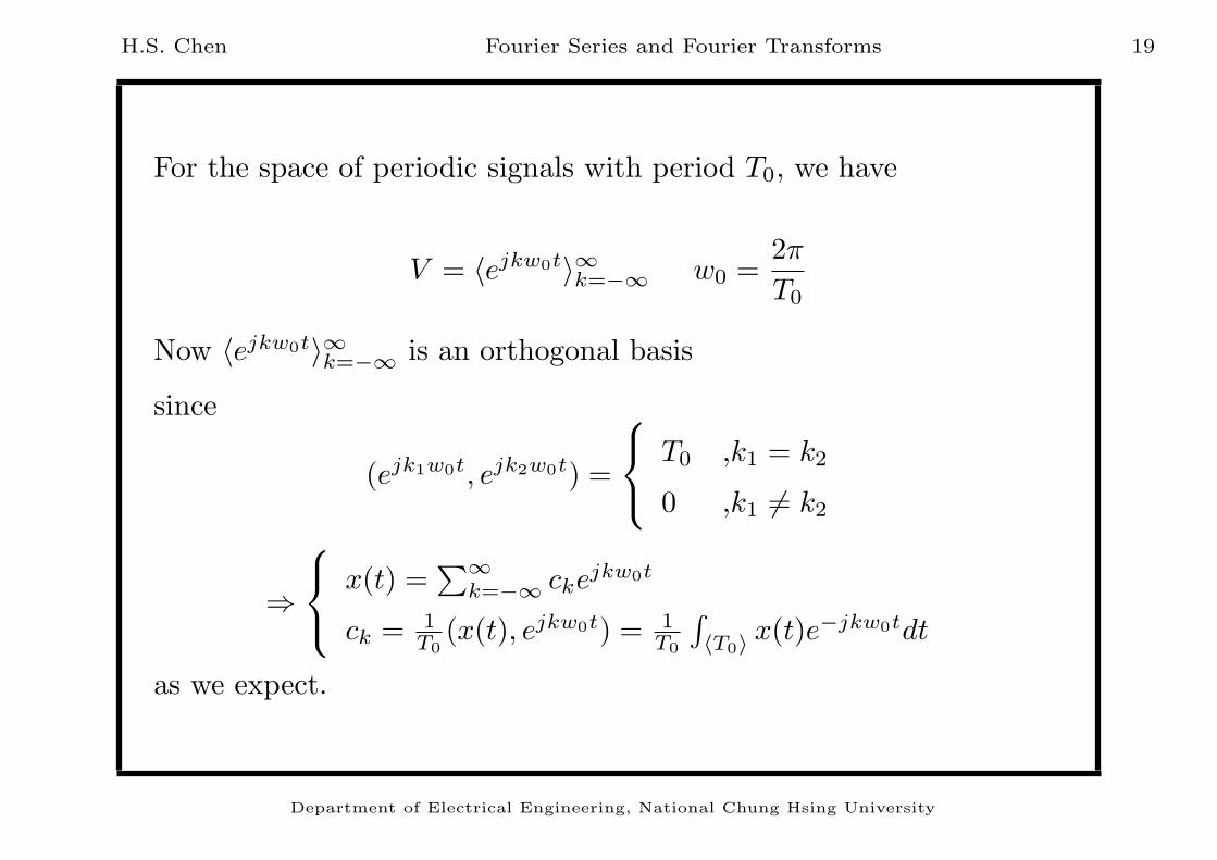
For the space of periodic signals with period T0, we have

V = 〈ejkw0t〉∞k=−∞ w0 =2π

T0

Now 〈ejkw0t〉∞k=−∞ is an orthogonal basis

since

(ejk1w0t, ejk2w0t) =

T0 ,k1 = k2

0 ,k1 6= k2

⇒

x(t) =∑∞

k=−∞ ckejkw0t

ck = 1T0

(x(t), ejkw0t) = 1T0

∫

〈T0〉x(t)e−jkw0tdt

as we expect.



• If x(t) is real, we can use {cos(kw0t), sin(kw0t)}∞k=0 as the

orthogonal basis for x(t).

Original basis:

{ejkw0t}∞k=−∞

Since

ejkw0t+e−jkw0t

2 = cos(kw0t)

ejkw0t−e−jkw0t

2j = sin(kw0t)

we can replace {ejkw0t, e−jkw0t}∞k=1 by {cos(kw0t), sin(kw0t)}∞k=1



Now if x(t) is real, we have

ck =1

T0

∫ T0

0

x(t)e−jkw0tdt

c−k =1

T0

∫ T0

0

x(t)e−j(−k)w0tdt

=1

T0

∫ T0

0

x(t)ejkw0tdt

= (1

T0

∫ T0

0

x(t)e−jkw0tdt)∗

= c∗k

= |ck|e−j∠c−k

i.e. c−k = |c−k|ej∠c−k = |ck|e

−j∠ck⇒ |c−k| = |ck| and ∠c−k = −∠ck



x(t) =

∞∑

k=−∞

ckejkw0t

= c0 +

−1∑

k=−∞

ckejkw0t +

∞∑

k=1

ckejkw0t

= c0 +

∞∑

k=1

c−ke−jkw0t +

∞∑

k=1

ckejkw0t

= c0 +

∞∑

k=1

(c∗−ke−jkw0t)∗ +

∞∑

k=1

ckejkw0t

= c0 +

∞∑

k=1

[(cke−jkw0t)∗ + ckejkw0t]



= c0 +

∞∑

k=1

2Re{ckejkw0t}

= c0 +

∞∑

k=1

2Re{(Re{ck}+ jIm{ck})(cos(kw0t) + jsin(kw0t))}

= c0 +

∞∑

k=1

2(Re{ck}cos(kw0t)− Im{ck}sinkw0t)



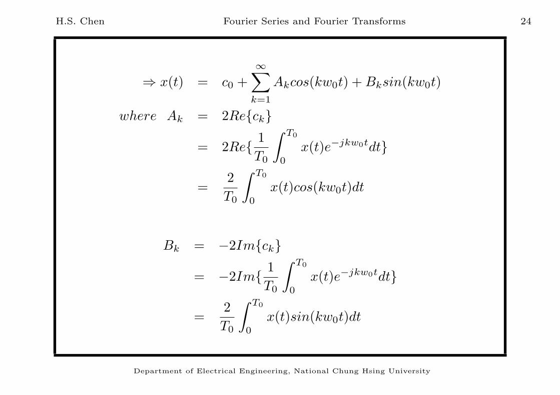
⇒ x(t) = c0 +

∞∑

k=1

Akcos(kw0t) + Bksin(kw0t)

where Ak = 2Re{ck}

= 2Re{1

T0

∫ T0

0

x(t)e−jkw0tdt}

=2

T0

∫ T0

0

x(t)cos(kw0t)dt

Bk = −2Im{ck}

= −2Im{1

T0

∫ T0

0

x(t)e−jkw0tdt}

=2

T0

∫ T0

0

x(t)sin(kw0t)dt



Properties of Fourier Series

x(t)FS;w0←→ ak

y(t)FS;w0←→ bk

1.linearity

⇒ Ax(t) + By(t)FS;w0←→ Aak + Bbk

c(t) =∞∑

k=−∞

ckejkw0t



and

c(t) = Ax(t) + By(t) = A∑

k

akejkw0t + B∑

k

bkejkw0t

=∑

k

(Aak + Bbk)ejkw0t

⇒ ck = Aak + Bbk



2. time shifting

x(t)↔ ak

x(t− t0)↔ ake−jkw0t0

︸︷︷︸

bk

bk =1

T

∫

〈T 〉

x(t− t0)e−jkw0tdt

=1

T

∫ T

0

x(t− t0)e−jkw0tdt

=1

T

∫ T−t0

−t0

x(τ)e−jkw0(τ+t0)dτ

= (1

T

∫

〈T 〉

x(τ)e−jkw0τdτ)e−jkw0t0

= ake−jkw0t0



3. frequency shifting

x(t)↔ ak

x(t)ejMw0t ↔ bk = ak−M

bk =1

T

∫

〈T 〉

x(t)ejMw0te−jkw0tdt =1

T

∫

〈T 〉

x(t)e−j(k−M)w0tdt

= ak−M



4. conjugation

x(t)↔ ak

x∗(t)↔ bk = a∗−k

bk =1

T

∫

〈T 〉

x∗(t)e−jkw0tdt = (1

T

∫

〈T 〉

x(t)e−j(−k)w0tdt)∗ = a∗−k

in particular if x(t) is real ⇒ x(t) = x∗(t)

therefore ak = a∗−k



5. multiplication

x(t)↔ ak

y(t)↔ bk

x(t)y(t)↔ ak ∗ bk = hk

i.e. hk =

∞∑

l=−∞

albk−l

x(t) =∞∑

k=−∞

akejkw0t

y(t) =

∞∑

l=−∞

blejlw0t



Finally, we have

x(t)y(t) =

∞∑

k=−∞

∞∑

l=−∞

akblej(k+l)w0t

=

∞∑

m=−∞

(

∞∑

l=−∞

am−lbl)ejmw0t

=

∞∑

m=−∞

hmejmw0t

where m = k + l.



6. convolution

z(t) = x(t) ∗ y(t)↔ zk = T0akbk

proof:

z(t) = x(t) ∗ y(t) =

∫

τ∈〈T0〉

x(τ)y(t− τ)dτ

⇒ zk =1

T0

∫

t∈〈T0〉

z(t)e−jkw0tdt

=1

T0

∫

t∈〈T0〉

∫

τ∈〈T0〉

x(τ)y(t− τ)dτe−jkw0tdt

=1

T0

∫

τ∈〈T0〉

x(τ)

∫

t∈〈T0〉

y(t− τ)e−jkw0tdtdτ

= T01

T0

∫

τ∈〈T0〉

x(τ)e−jkw0τdτ1

T0

∫

λ∈〈T0〉

y(λ)e−jkw0λdλ

= T0akbk



7. Parseval’s theorem for F.S.

P =1

T0

∫ T0

0

|x(t)|2dt =

∞∑

k=−∞

|ck|2

I.e., to find the average power P of x(t), we can either calculate in

time domain or in frequency domain.



proof:

1

T0

∫ T0

0

|x(t)|2dt

=1

T0

∫ T

0

∞∑

k=−∞

ckejkw0t∞∑

m=−∞

c∗me−jmw0tdt

=1

T0

∞∑

k=−∞

∞∑

m=−∞

ckc∗m

∫

〈T0〉

ej(k−m)w0tdt

=1

T0

∞∑

k=−∞

ckc∗kT0

=∞∑

k=−∞

|ck|2



For real signal x(t), we have |c−k| = |ck|

⇒ P = |c0|2 + 2

∞∑

k=1

|ck|2

also we have

Ak = 2Re{ck}

Bk = −2Im{ck}

therefore

|ck|2 = Re2{ck}+ Im2{ck} =

A2k

4+

B2k

4



Finally for real signal, we have another form:

P = |c0|2 +

∞∑

k=1

A2k

2+

B2k

2



FT

We will do the following step by step

1. The derivation of FT

2. Some examples of FT

3. Properties of FT



Fourier Transform: from F.S. to F.T.

f(t)FT←→ F (jw)

F (jw) = F{f(t)} and f(t) = F−1{f(jw)}

F (jw) =∫ ∞

−∞f(t)e−jwtdt

f(t) = 12π

∫ ∞

−∞F (jw)ejwtdw



Fourier transform pair for some common signals

Example 1:

f(t) =

1, −T1 ≤ t ≤ T1

0, otherwise



F (jw) =

∫ ∞

−∞

f(t)e−jwtdt

=

∫ T1

−T1

1 · e−jwtdt

=1

−jwe−jwt|T1

−T1

=1

+jw(ejT1w−e−jT1w

)

=2T1

wT1

ejT1w − e−jT1w

2j

= 2T1sin(T1w)

wT1

= 2T1sinc(T1w)

therefore F(jw) is the envelop function of T0 · Ck



i.e.

rect(t

w)←→Wsinc(

wW

2)



Example 2: x(t) = e−atu(t) (a > 0)

=⇒ X(jw) =

∫ ∞

−∞

x(t)e−jwtdt

=

∫ ∞

−∞

e−atu(t)e−jwtdt

=

∫ ∞

0

e−(jw+a)tdt

=1

−(jw + a)e−(jw+a)t|0−∞

=1

jw + a(ifa > 0)



Example 3: x(t) = e−a|t| (a > 0)



=⇒ X(jw) =

∫ ∞

−∞

x(t)e−jwtdt

=

∫ ∞

−∞

e−a|t|e−jwtdt

=

∫ 0

−∞

eate−jwtdt +

∫ ∞

0

e−ate−jwtdt

=

∫ 0

−∞

e(a−jw)tdt +

∫ ∞

0

e−(a+jw)tdt

=1

a− jwe(a−jw)t|∞0 +

1

jw + a

=1

a− jw+

1

jw + aif a > 0

=2a

a2 + w2if a > 0



Example 4:

x(t) = δ(t)

=⇒ X(jw) =

∫ ∞

−∞

x(t)e−jwtdt

=

∫ ∞

−∞

δ(t)e−jwtdt = e−jwt|t=0 = 1

i.e.

δ(t)←→ 1

similarly if x(t) = δ(t− t0)

=⇒ X(jw) =

∫ ∞

−∞

δ(t− t0)e−jwtdt

= e−jwt|t=t0 = e−jwt0

δ(t− t0)←→ 1 · e−jwt0



Example 5:

X(jw) = 2πδ(w)

=⇒ x(t) =1

2π

∫ ∞

−∞

X(jw)ejwtdw

=1

2π

∫ ∞

−∞

2πδ(w)ejwtdw

= ejwt|w=0 = 1

i.e.

1←→ 2πδ(w)

similarly if X(jw) = 2πδ(w − w0)

=⇒ x(t) =1

2π

∫ ∞

−∞

2πδ(w − w0)ejwtdw

= ejwt|w=w0= ejw0t



i.e.

1 · ejw0t ←→ 2πδ(w − w0) (frequency shifting) )

With this, we can represent the periodic signal by FT:

x(t) =

∞∑

k=−∞

Ckejkw0t

=⇒ X(jw) = F{x(t)} = F{

∞∑

k=−∞

Ckejkw0t}

=

∞∑

k=−∞

CkF{ejkw0t}

=∞∑

k=−∞

2πCkδ(w − kw0)



i.e.



Example 6:

x(t) = cosw0t =1

2ejw0t +

1

2e−jw0t

=⇒ X(jw) =1

22πδ(w − w0) +

1

22πδ(w + w0)

= πδ(w − w0) + πδ(w + w0)

x(t) = sinw0t =1

2jejw0t −

1

2je−jw0t

=⇒ X(jw) =1

2j2πδ(w − w0)−

1

2j2πδ(w + w0)

= jπδ(w + w0)− jπδ(w − w0)



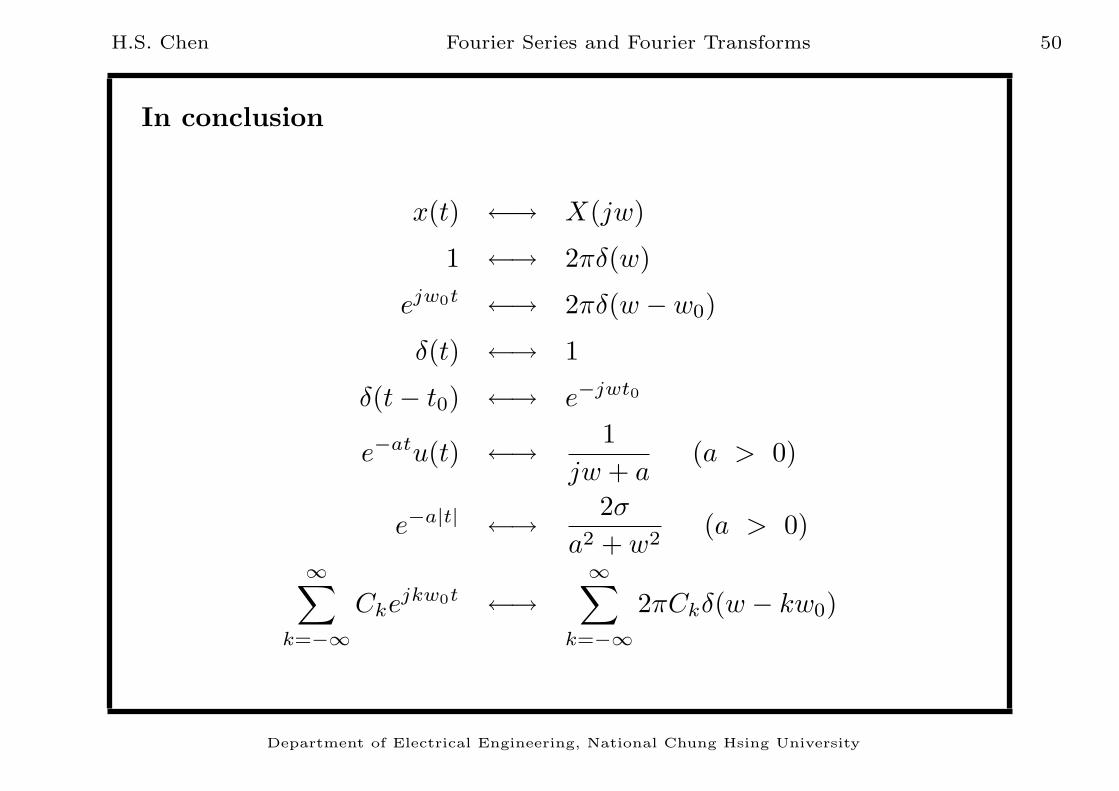
In conclusion

x(t) ←→ X(jw)

1 ←→ 2πδ(w)

ejw0t ←→ 2πδ(w − w0)

δ(t) ←→ 1

δ(t− t0) ←→ e−jwt0

e−atu(t) ←→1

jw + a(a > 0)

e−a|t| ←→2σ

a2 + w2(a > 0)

∞∑

k=−∞

Ckejkw0t ←→∞∑

k=−∞

2πCkδ(w − kw0)



cosw0t ←→ πδ(w + w0) + πδ(w − w0)

sinw0t ←→π

jδ(w − w0)−

π

jδ(w + w0)

u(t) ←→ πδ(w) +1

jw

sgn(t) ←→2

jw



Properties of FT

x(t) ←→ X(jw)

y(t) ←→ Y (jw)

ax(t) + by(t) ←→ aX(jw) + bY (jw)

x∗(t) ←→ X∗(−jw)

x(at) ←→1

|a|X(

w

a)

x(t− t0) ←→ X(jw)e−jwt0

x(t)ejw0t ←→ X(j(w − w0))

X(t) ←→ 2πx(−w)



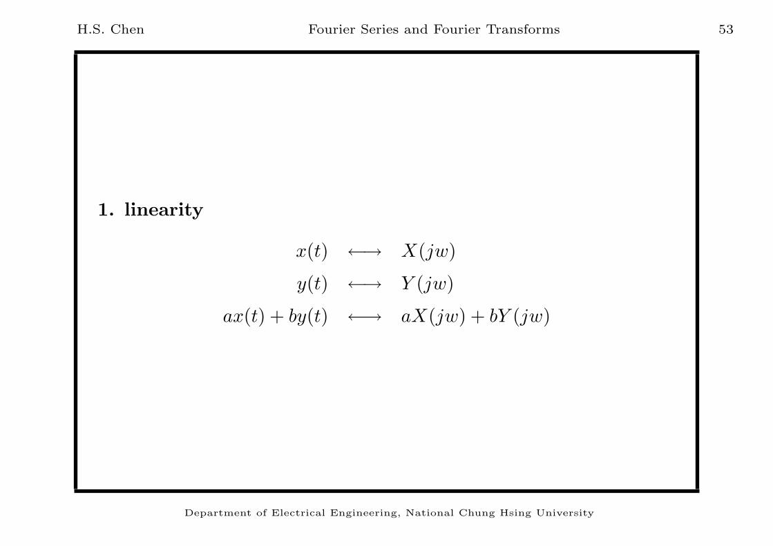
1. linearity

x(t) ←→ X(jw)

y(t) ←→ Y (jw)

ax(t) + by(t) ←→ aX(jw) + bY (jw)



2. conjugation

x(t) ←→ X(jw)

x∗(t) ←→ X∗(−jw)

∫ ∞

−∞

x∗(t)e−jwtdt = (

∫ ∞

−∞

x(t)e−(−jwt))∗ = X∗(−jw)

if x(t) = x∗(t) real =⇒ X∗(−jw) = X(jw)

=⇒

Re{X(−jw)} = Re{X(jw)}

Im{X(−jw)} = −Im{X(jw)}

|X(−jw)| = |X(jw)|

∠X(−jw) = −∠X(−jw)



3. Time scaling

f(αt)F←→

1

|α|F (

w

α)

Interpretation:

• If α > 1, we obtain that compression in the time domain

corresponds to expansion in the frequency domain.

• If 0 < α < 1, we obtain that compression in the time domain

corresponds to expansion in the frequency domain.



4. Time shifting

f(t− t0)F←→ e−jwt0F (w)



Example: Recall the Fourier transforms of δ(t) and δ(t− t0).

Proof:

F [f(t− t0)] =

∫ ∞

−∞

f(t− t0)e−jwtdt

=

∫ ∞

−∞

f(σ)e−jw(σ+t0)dσ

= e−jwt0F (w)



Combining Time Scaling and Time shifting :

f(at + t0)F←→

1

|a|F (

w

a)e+jt0w/a

This is obtained by (i) shifting f(t) by t0 and (ii) scaling the result of

(i) by a.



5. Frequency shifting

ejw0tf(t)F←→ F (w − w0)

for any real w0.

Example: Recall the Fourier transforms of 1 and ejw0t, and u(t) and

cos(w0t)u(t). Also ,examine the ”modulation” property below.



Proof:

F [ejw0tf(t)] =

∫ ∞

−∞

ejw0tf(t)e−jwtdt

=

∫ ∞

−∞

f(t)e−j(w−w0)tdt

= F (w − w0)



6. Duality

F (−t)←→ 2πf(w)

F (t)←→ 2πf(−w)



Proof:

f(t) =1

2π

∫ ∞

−∞

F (w)ejwtdw

2πf(−t) =

∫ ∞

−∞

F (w)e−jwtdw

2πf(−w) =

∫ ∞

−∞

F (t)e−jwtdt = F [F (t)]

where the last line is obtained by interchanging t with w.



7. Convolution

If all the involved Fourier transforms exist, then

x(t) ∗ h(t) F←→ X(w)H(w)



Proof:

F [x(t) ∗ h(t)] =

∫ ∞

−∞

[

∫ ∞

−∞

h(t− τ)x(τ)dτ ]e−jwtdt

=

∫ ∞

−∞

x(τ)[

∫ ∞

−∞

h(t− τ)e−jwtdt]dτ

=

∫ ∞

−∞

x(τ)[e−jwtH(w)]dτ

= H(w)

∫ ∞

−∞

x(τ)e−jwtdτ

= H(w)X(w)



8. Modulation

If all the involved Fourier transforms exist, then

x(t)m(t)F←→

1

2πX(w) ∗M(w)



Proof:

F [x(t)m(t)] =

∫ ∞

−∞

x(t)[1

2π

∫ ∞

−∞

M(w′)ejw′tdw′]e−jwtdt

=1

2π

∫ ∞

−∞

M(w′)[

∫ ∞

−∞

x(t)e−jwte+jw′tdt]dw′

=1

2π

∫ ∞

−∞

M(w′)[X(w − w′)]dw′

=1

2πM(w) ∗X(w)

Example: This result can be used to calculate F [cos(w0t)u(t)].



9. Time Differentiation

If f(t) is continuous and if f(t) and f ′(t) = df(t)dt are both absolutely

integrable (and thus satisfy the Dirichlet conditions),then

df(t)

dt

F←→ jwF (w)



Proof:∫ ∞

−∞

f ′(t)e−jwtdt = f(t)e−jwt|∞−∞ + jw

∫ ∞

−∞

f(t)e−jwtdt

The key step now is to observe that since f(t) is assumed to be

absolutely integrable, then f(t)→ 0 as t→ ±∞ and thus the first

term on the RHS evaluates to zero. The second term is simply

jwF (w)



10. Parseval’s Theorem

Parseval’s Theorem∫ ∞

−∞

|f(t)|2dt =1

2π

∫ ∞

−∞

|F (w)|2dw



Proof:∫ ∞

−∞

|f(t)|2dt =

∫ ∞

−∞

f(t)f∗(t)dt

=

∫ ∞

−∞

f(t)[1

2π

∫ ∞

−∞

F ∗(w)e−jwtdw]dt

=1

2π

∫ ∞

−∞

F ∗(w)[

∫ ∞

−∞

f(t)e−jwtdt]dw

=1

2π

∫ ∞

−∞

F ∗(w)F (w)dw

=1

2π

∫ ∞

−∞

|F (w)|2dw


fourier series and fourier transforms -...

Documents