Name Date ----------~----------------- ------------------

Fourier Theory-Frequency Domain and Time Domain

OBJECTIVES

1. Learn how a square wave can be produced from a series of sine waves at different frequencies and amplitudes.

2. Learn how a triangular wave can be produced from a series of cosine waves at different frequencies and amplitudes.

3. Learn about the difference between curve plots in the time domain and the frequency domain.

4. Examine periodic pulses with different duty cycles in the time domain and in the frequency domain.

5. Examine what happens to periodic pulses with different duty cycles when passed through a low-pass filter when the filter cutoff frequency is varied.

MATERIALS

One function generator One oscilloscope One spectrum analyzer One LM 741 op-amp Two 5 nF variable capacitors Resistors: 5.86 kn, 10 kn, and 30 kQ

THEORY

Communications systems are normally studied using sinusoidal voltage waveforms to simplify the analysis. In the real world, electrical information signals are normally nonsinusoidal voltage waveforms, such as audio signals, video signals, or computer data. Fourier theory provides a powerful means of analyzing communications systems by representing a nonsinusoidal signal as a series of sinusoidal voltages added together. Fourier theory states that a complex voltage waveform is essentially a composite of harmonically related sine or cosine waves at different

53

,. i

frequencies and amplitudes determined by the particular signal voltage waveshape. Any nonsinusoidal periodic waveform can be broken down into a sine or cosine wave equal to the frequency ofthe periodic waveform, called the fundamental frequency, and a series of sine or cosine waves that are integer mUltiples of the fundamental frequency, called harmonics. This series of sine or cosine waves is called a Fourier series.

Most of the signals analyzed in a communications system are expressed in the time domain, meaning that the voltage, current, or power is plotted as a function oftime. The voltage, current, or power is represented on the vertical axis and time is represented on the horizontal axis. Fourier theory provides a new way of expressing signals in the frequency domain, meaning that the voltage, current, or power is plotted as a function of frequency. Complex signals containing many sine or cosine wave components are expressed as sine or cosine wave amplitudes at different frequencies, with amplitude represented on the vertical axis and frequency represented on the horizontal axis. The length of each of a series of vertical straight lines represents the sine or cosine wave amplitudes, and the location of each line along the horizontal axis represents the sine or cosine wave frequencies. This is called a frequency spectrum. In many cases the frequency domain is more useful than the time domain because it reveals the bandwidth requirements of the communications system in order to pass the signal with minimal distortion. Test instruments for displaying signals in both the time domain and the frequency domain are available. The oscilloscope is used to display signals in the time domain and the spectrum analyzer is used to display the frequency spectrum of signals in the frequency domain.

In the frequency domain, normally the harmonics decrease in amplitude as their frequency gets higher until the amplitude becomes negligible. The more harmonics added to make up the composite waveshape, the more the composite waveshape will look like the original waveshape. Because it is impossible to design a communications system that will pass an infinite number of frequencies (infinite bandwidth), a perfect reproduction of an original signal is impossible. In most cases, eliminating some ofthe harmonics does not significantly alter the original waveform. The more information contained in a signal voltage waveform (faster changing voltages), the larger the number of high-frequency harmonics required to reproduce the original waveform. Therefore, the more complex the signal waveform (the faster the voltage changes), the wider the bandwidth required to pass it with minimal distortion. A formal relationship between bandwidth and the amount of information communicated is called Hartley's law, which states that the amount of information communicated is proportional to the bandwidth of the communications system and the transmission time.

Because much of the information communicated today is digital, the accurate transmission of binary pulses through a communications system is important. Fourier analysis of binary pulses is especially useful in communications because it provides a way to determine the bandwidth required for the accurate transmission of digital data. Although, theoretically, the communications system must pass all of the harmonics of a pulse waveshape, in reality, relatively few of the harmonics are needed to preserve the waveshape.

54

Tf ..

The duty cycle of a series of periodic pulses is equal to the ratio ofthe pulse up time (to) to the time period of one cycle (T) expressed as a percentage. Therefore,

t D=...E...xlOO%

T

In the special case where a series of periodic pulses has a 50% duty cycle, called a square wave, the plot in the frequency domain will consist of a fundamental and all odd harmonics, with the even harmonics missing. The fundamental frequency will be equal to the frequency of the square wave. The amplitude of each odd harmonic will decrease in direct proportion to the odd harmonic frequency. Therefore,

v(t) = Asin27ifi + A sin(3)27ifi + A sin (5)27ifi + A sin(7)27tfi- - __ -- __ _ 357

The circuit in Figure 5-1 will generate a square wave voltage by adding a series of sine wave voltages as specified above. As the number of harmonics is decreased, the square wave that is produced will have more ripples. An infinite number of harmonics would be required to produce a perfectly flat square wave.

Figure 5-1 Square Wave Fourier Series

10V oc

III 10kOhm Key=A 'VV"v 0---0-

10kOhm Key=B 0-

3.33V 3kHz OOeg f3

10kOhm Key=C

0-

2V 5kHz ODeg f5

1OkOhm Key = 0

0-

1.43V 7kHz OOeg f7

Key=E r----------~~v_------~ 0-

10kOhm

1.11V 9kHz ODeg f9

10kOhm Key=F

0-

XSC1

1000hm

55

The circuit in Figure 5-2 will generate a triangular wave voltage by adding a series of cosine wave voltages. In order to generate a triangular wave, each harmonic frequency must be an odd multiple of the fundamental frequency with no even harmonics. The fundamental frequency will be equal to the frequency ofthe triangular wave. The amplitude of each odd harmonic will decrease in direct proportion to the square of the odd harmonic frequency. Therefore,

A A v(t) = Acos27ift + )Tcos(3)27ift + "52COS(5)27tjt + - --------

Whenever a dc voltage is added to a periodic time varying voltage, the waveshape will be shifted up by the amount of the dc voltage.

Figure 5-2

15V DC

Triangular Wave Fourier Series

r-----Illt-I-----~

10kOhm Key=B 0-

1.11V 3kHz 90Deg f3 10kOhm Key=C

0-

O.4V 5kHz 90Deg f5 10kOhm Key=D

0-

O.2V 7kHz 90Deg f7

1OkOhm Key=E 0-

XSC1

1000hm

For a series of periodic pulses with other than a 50% duty cycle, the plot in the frequency domain will consist of a fundamental and even and odd harmonics. The fundamental frequency will be equal to the frequency ofthe periodic pulse train. The amplitude (A) of each harmonic will depend on the value of the duty cycle. A general frequency domain plot of a periodic pulse train with a duty cycle other than 50% is shown in the figure on page 57. The outline of the peaks of the individual frequency components is called the envelope of the frequency spectrum. The first zero-amplitude frequency crossing point is labeled fo = lito, where to is the up time of the pulse train. This first zero-amplitude frequency crossing point (fo) detennines the minimum bandwidth (BW) required for passing the pulse train with minimal distortion.

56

Therefore,

A

I ~ I fo=l/to

1 BW =;; =-

o t o

2/to

Frequency Spectrum of a Pulse Train

f

Notice that the lower the value of to, the wider the bandwidth required to pass the pulse train with minimal distortion. Also note that the separation of the lines in the frequency spectrum is equal to the inverse of the time period (lIT) of the pulse train. Therefore a higher frequency pulse train requires a wider bandwidth (BW) because f= lIT.

The circuit in Figure 5-3 will demonstrate the difference between the time domain and the frequency domain. It will also demonstrate how filtering out some of the harmonics affects the output waveshape compared to the original input waveshape. The frequency generator (XFG1) will generate a periodic pulse waveform applied to the input of the filter (5). At the output of the filter (7), the oscilloscope will display the periodic pulse waveform in the time domain, and the spectrum analyzer will display the frequency spectrum of the periodic pulse waveform in the frequency domain. The Bode plotter will display the Bode plot of the filter so that the filter bandwidth can be measured. The filter is a 2-pole low-pass Butterwoth active filter using a 741 op-amp.

57

Figure 5-3 Time Domain and Frequency Domain

5

XFG1

30kOhm R

30kOhm R

5nF Key = a

. C 5%

~ 1 · ;~~=b -=- C 5%

3

6

2 741

5.86kOhm R1

10kOhm R2

7

PROCEDURE

Step 1 Open circuit file FIGS-I. Make sure that the following oscilloscope settings are selected: Time base (Scale = 200 uslDiv, Xpos = 0, Yff), Ch A (Scale = 5 VlDiv, Ypos = 0, DC), Ch B (Scale = 50 mVlDiv, Ypos = 0, DC), Trigger (pos edge, Level = 0, Auto). You will generate a square wave curve plot on the oscilloscope screen from a series of sine waves called a Fourier series.

Note: It is difficult to perform these steps in a hardwired lab environment because a number of frequency generators are needed to generate a series of sinusoidal functions at different frequencies.

Step 2

58

Run the simulation. Notice that you have generated a square wave curve plot on the oscilloscope screen (blue curve) from a series of sine waves. Notice that you have also plotted the fundamental sine wave (red). Draw the square wave (blue) curve plot and the fundamental sine wave (red) curve plot in the space provided on page 59.

Step 3

Step 4

I

Use the cursors to measure the time period for one cycle (T) of the square wave (blue) and the fundamental sine wave (red) and show the value ofT on the curve plot.

Calculate the frequency (f) of the square wave and the fundamental sine wave from the time period (T).

Questions: What is the relationship between the fundamental sine wave frequency and the square wave fr,equency (f)?

What is therelationship between the sine wave harmonic frequencies (frequencies of sine wave generators f3, fs, f7, and f9 in Figure 5-1) and the sine wave fundamental frequency (fl)?

59

What is the relationship between the amplitude of each ofthe hannonic sine wave generators and the amplitude of the fundamental sine wave generator?

StepS Press the A key to close switch A to add a dc voltage level to the square wave curve plot. (If the switch does not close, click the mouse arrow in the circuit window before pressing the A key). Run the simulation again. Change the oscilloscope settings as needed. Draw the new square wave (blue) curve plot in the space provided.

.

Question: What happened to the square wave curve plot? Explain why.

60

Step 6

Step 7

Step 8

Press the F and E keys to open switches F and E to eliminate the ninth and seventh harmonic sine waves. Run the simulation again. Draw the new curve plot (blue) in the space provided. Note any change on the graph.

1 11 II I ----+- I I i I

. I I 1--1-I

. -1----1 ---- ----+------f--+---+------f--+---+---!---t--I I I I ' i -l-------r--+-+----+---+-+---+---+-+---+--

-J--r---J----+-I---+---!-----+--+---+--+----+----+-___+__

Press the D key to open switch D to eliminate the fifth harmonic sine wave. Run the simulation again. Draw the new curve plot (blue) in the space provided. Note any change on the graph.

--~-r I I

I --- -- ---t----+----+-- +---+--

Press the C key to open switch C and eliminate the third harmonic sine wave. Run the simulation again.

61

Question: What happened to the square wave curve plot? Explain.

Step 9 Open circuit file FIG5-2. Make sure that the following oscilloscope settings are selected: Time base (Scale = 200 uslDiv, Xpos = 0, Y/T), Ch A (Scale = 5 VlDiv, Ypos = 0, DC), Ch B (Scale = 100 mVlDiv, Ypos = 0, DC), Trigger (pos edge, Level = 0, Auto ). You will generate a triangular wave curve plot on the oscilloscope screen from a series of cosine waves called a Fourier series.

Note: It is difficult to perform these steps in a hardwired lab environment because a number of frequency generators are needed to generate a series of sinusoidal functions at different frequencies.

Step 10 Run the simulation. Notice that you have generated a triangular wave curve plot on the oscilloscope screen (blue curve) from a series of cosine waves. Notice that you have also plotted the fundamental cosine wave (red). Draw the triangular wave (blue) curve plot and the fundamental cosine wave (red) curve plot in the space provided.

I

Step 11 Use the cursors to measure the time period for one cycle (T) of the triangular wave (blue) and the fundamental (red), and show the value ofT on the curve plot.

62

Step 12 Calculate the frequency (f) of the triangular wave from the time period (T).

Questions: What is the relationship between the fundamental frequency and the triangular wave frequency?

What is the relationship between the harmonic frequencies (frequency of generators f3, f5, and f7 in Figure 5-2) and the fundamental frequency (fJ)?

What is the relationship between the amplitude of each of the harmonic generators and the amplitude of the fundamental generator?

Step 13 Press the A key to close switch A to add a dc voltage level to the triangular wave curve plot. Run the simulation again. Draw the new triangular wave (blue) curve plot in the space provided.

63

Question: What happened to the triangular wave cmve plot? Explain.

Step 14 Press the E and D keys to open switches E and D to eliminate the seventh and fifth hannonic sine waves. Run the simulation again. Draw the new cmve plot (blue) in the space provided. Note any change on the graph.

i

I I I I

I I I I i i J

I I I

I

I , ! J

Step 15 Press the C key to open switch C to eliminate the third hannonic sine wave. Run the simulation again.

Question: What happened to the triangular wave cmve plot? Explain.

Step 16 Open circuit file FIG5-3. Make sure that the following function generator settings are selected: Square wave, Freq = 1 kHz, Duty cycle = 50%, Ampl = 2.5 V, Offset = 2.5 V. Make sure that the following oscilloscope settings are selected: Time base (Scale = 500 uslDiv, Xpos = 0, YIT), Ch A (Scale = 5 VlDiv, Ypos = 0, DC), Ch B (Scale = 5 VlDiv, Ypos = 0, DC), Trigger (pos edge, Level = 0, Auto). You will plot a square wave in the time domain at the input and output of a two-pole low-pass Butterworth filter.

64

Step 17 Bring down the oscilloscope enlargement and run the simulation to one full screen display, then pause the simulation. Notice that you are displaying square wave curve plots in the time domain (voltage as a function of time). The red curve plot is the filter input (5) and the blue curve plot is the filter output (7).

Question: Are the filter input (red) and output (blue) curve plots the same shape, disregarding any amplitude differences?

Step 18 Use the cursors to measure the time period (T) and the up time (to) of the input curve plot (red) and record the values.

T= to= ----- -----

Step 19 Calculate the pulse duty cycle (D) from to and T.

Question: How did your calculated duty cycle compare with the duty cycle setting on the function generator?

Step 20 Bring down the Bode plotter enlargement to display the Bode plot ofthe filter. Make sure that the following Bode plotter settings are selected: Magnitude, Vertical (Log, F = 10 dB, I = -40 dB), Horizontal (Log, F = 200 kHz, I = 100 Hz). Run the simulation to completion. Use the cursor to measure the cutoff frequency (fe) of the low-pass filter and record the value.

fe= ____ _

Note: The following steps carmot be performed in a hardwired lab environment unless a spectrum analyzer is available.

Step 21 Bring down the spectrum analyzer enlargement. Make sure that the following spectrum analyzer settings are selected: Freq (Start = 0 kHz,Center = 5 kHz, End = 10kHz), Ampl (Lin, Range = 1 VlDiv), Res = 50 Hz. Run the simulation until the Resolution Frequencies match, then pause the simulation. Notice that you have displayed the filter output square wave frequency spectrum in the frequency domain. Use the cursor to measure the amplitude of the fundamental and each harmonic to the ninth and record your answers in Table 5-1.

65

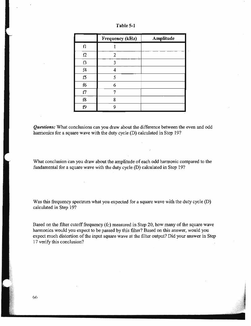
Table 5-1

Frequency (kHz) Amplitude

f1 1

f2 2

f3 3

f4 4

f5 5

f6 6

fl 7

f8 8

f9 9

Questions: What conclusions can you draw about the difference between the even and odd hannonics for a square wave with the duty cycle (D) calculated in Step 19?

What conclusion can you draw about the amplitude of each odd hannonic compared to the fundamental for a square wave with the duty cycle (D) calculated in Step 19?

Was this frequency spectrum what you expected for a square wave with the duty cycle (D) calculated in Step 19?

Based on the filter cutoff frequency (fc) measured in Step 20, how many of the square wave harmonics would you expect to be passed by this filter? Based on this answer, would you expect much distortion of the input square wave at the filter output? Did your answer in Step 17 verify this conclusion?

66

Step 22 Adjust both filter capacitors (C) to 50% (2.5 nF) each. (Ifthe capacitors won't change, click the mouse arrow in the circuit window). Bring down the oscilloscope enlargement and run the simulation to one full screen display, then pause the simulation. The red curve plot is the filter input and the blue curve plot is the filter output.

Question: Are the filter input (red) and output (blue) curve plots the same shape, disregarding any amplitude differences?

Step 23 Bring down the Bode plotter enlargement to display the Bode plot of the filter. Use the cursor to measure the cutoff frequency (fc) of the low-pass filter and record the value.

fc= ____ _

Step 24 Bring down the spectrum analyzer enlargement to display the filter output frequency spectrum in the frequency domain. Run the simulation until the Resolution Frequencies match, then pause the simulation. Use the cursor to measure the amplitude of the fundamental and each harmonic to the ninth and record your answers in Table 5-2. .

Table 5-2

Frequency (kHz) Amplitude

fl 1

f2 2

f3 3

f4 4

f5 5

f6 6

f7 7

f8 8

19 9

Questions: How did the amplitude of each harmonic in Table 5-2 compare with the values in Table 5-1?

67

Based on the filter cutoff frequency (fc), how many of the square wave harmonics should be passed by this filter? Based on this answer, would you expect much distortion of the input square wave at the filter output? Did your answer in Step 22 verify this conclusion?

Step 25 Change both capacitors (C) back to 5% (0.25 nF). Change the duty cycle to 20% on the function generator. Bring down the oscilloscope enlargement and run the simulation to one full screen display, then pause the simulation. Notice that you have displayed a pulse curve plot on the oscilloscope in the time domain (voltage as a function oftime). The red curve plot is the filter input and the blue curve plot is the filter output.

Question: Are the filter input (red) and output (blue) curve plots the same shape, disregarding any amplitude differences?

Step 26 Use the cursors to measure the time period (T) and the up time (to) of the input curve plot (red) and record the values.

T= ----- to= -----

Step 27 Calculate the input pulse duty cycle (D) from to and T.

Question: How did your calculated duty cycle compare with the duty cycle setting on the function generator?

Step 28 Bring down the Bode plotter enlargement to display the Bode plot of the filter.

68

Use the cursor to measure the cutoff frequency (fc) of the low-pass filter and record the value.

fc = -----

Step 29 Bring down the spectrum analyzer enlargement to display the filter output frequency spectrum in the frequency domain. Run the simulation until the Resolution Frequencies match, then pause the simulation. Draw the frequency plot in the space provided. Also draw the envelope . of the frequency spectrum.

Question: Is this the frequency spectrum you expected for a square wave with a duty cycle less than 50%?

Step 30 Use the cursor to measure the frequency of the first zero crossing point (fo) of the spectrum envelope and record your answer on the graph.

Step 31 Based on the value of to measured in Step 26, calculate the expected first zero crossing point (fo) of the spectrum envelope.

Question: How did your calculated value of fa compare the measured value on the curve plot?

Step 32 Based on the value of fo, calculate the minimum bandwidth (BW) required for the filter to pass the input pulse waveshape with minimal distortion.

Question: Based on this answer and the cutoff frequency (fc) of the low-pass filter measured in Step 28, would you expect much distortion of the input square wave at the filter output? Did your answer in Step 25 verify this conclusion?

Step 33 Adjust the filter capacitors (C) to 50% (2.5 nF) each. Bring down the oscilloscope enlargement and run the simulation to one full screen display, then pause the simulation. The red curve plot is the filter input and the blue curve plot is the filter output.

Question: Are the filter input (red) and output (blue) curve plots the same shape, disregarding any amplitude differences?

Step 34 Bring down the Bode plotter enlargement to display the Bode plot of the filter. Use the cursor to measure the cutoff frequency (fc) of the low-pass filter and record the value.

fc= ____ _

Questions: Was the cutoff frequency (fc) less than or greater than the minimum bandwidth (BW) required to pass the input pulse waveshape with minimal distortion as determined in Step 32?

Based on this answer, would you expect much distortion of the input pulse waveshape at the filter output? Did your answer in Step 33 verify this conclusion?

Step 35 Bring down the spectrum analyzer enlargement to display the filter output frequency spectrum in the frequency domain. Run the simulation until the Resolution Frequencies match, then pause the simulation.

Question: What is the difference between this frequency plot and the frequency plot in Step 29?

70