fpga implementation and performance comparison of a
TRANSCRIPT
Rochester Institute of Technology Rochester Institute of Technology
RIT Scholar Works RIT Scholar Works
Theses
3-2006
FPGA implementation and performance comparison of a FPGA implementation and performance comparison of a
Bayesian face detection system Bayesian face detection system
Christopher J. Rericha
Follow this and additional works at: https://scholarworks.rit.edu/theses
Recommended Citation Recommended Citation Rericha, Christopher J., "FPGA implementation and performance comparison of a Bayesian face detection system" (2006). Thesis. Rochester Institute of Technology. Accessed from
This Thesis is brought to you for free and open access by RIT Scholar Works. It has been accepted for inclusion in Theses by an authorized administrator of RIT Scholar Works. For more information, please contact [email protected].
FPGA Implementation and Performance Comparison of a
Bayesian Face Detection System
by
Christopher J. Rericha
A Thesis Submitted in Partial Fulfillment of the Requirements for the Degree of Master of Science in Computer Engineering
Supervised by
Associate Professor, Department of Computer Engineering Dr. Juan Cockburn Department of Computer Engineering Kate Gleason College of Engineering
Rochester Institute of Technology Rochester, New York
March 2006
Approved By:
Juan Cockburn Dr. Juan Cockburn Associate Professor, Department of Computer Engineering Primary Adviser
Andreas Savakis Dr. Andreas Savakis Professor, Department of Computer Engineering
Marcin Lukowiak Dr. Marcin Lukowiak Assistant Professor, Department of Computer Engineering
Thesis Release Permission Form
Rochester Institute of Technology
Kate Gleason College of Engineering
Title: FPGA Implementation and Performance Comparison of a Bayesian
Face Detection System
I, Christopher J. Rericha, hereby grant permission to the Wallace Memorial Library to
reproduce my thesis in whole or part.
Chris Rericha Christopher J. Rericha
Date

Dedication
To my wife, for her loving support,
to my parents, for teaching me to work hard,
and to Jesus Christ, without whom I would be nothing
in

Acknowledgments
Special thanks to my advisors for giving me their time, knowledge, and especially their
patience. Thanks to TomWarsaw for sharing his VHDL knowledge. Thanks also to those
who helped me create mappings for the images used; I would still be creating maps today
without their help. Portions of the research in this paper use the Color FERET database of
facial images collected under the FERET program [10].
iv
Abstract
Face detection has primarily been a software-based effort. A hardware-based approach can
provide significant speed-up over its software counterpart. Advances in transistor technol
ogy have made it possible to produce larger and faster FPGAs at more affordable prices.
Through VHDL and synthesis tools it is possible to rapidly develop a hardware-based so
lution to face detection on an FPGA.
This work analyzes and compares the performance of a feature-invariant face detection
method implemented in software and an FPGA. The primary components of the face detec
tor were a Bayesian classifier used to segment the image into skin and nonskin pixels, and
a direct least square elliptical fitting technique to determine if the skin region's shape has
elliptical characteristics similar to a face. The C++ implementation was benchmarked on
several high performance workstations, while the VHDL implementation was synthesized
for FPGAs from several Xilinx product lines.
The face detector used to compare software and hardware performance had a modest
correct detection rate of 48.6% and a false alarm rate of 29.7%. The elliptical-shape of
the region was determined to be an inaccurate approach for filtering out non-face skin
regions. The software-based face detector was capable of detecting faces within images of
approximately 378x567 pixels or less at 20 frames per second on Pentium 4 and PentiumD
systems. The FPGA-based implementation was capable of faster detection speeds; a speed
up of 3.33 was seen on a Spartan 3 and 4.52 on a Virtex 4. The comparison shows that an
FPGA-based face detector could provide a significant increase in computational speed.

Contents
Dedication iii
Acknowledgments iv
Abstract v
Glossary xi
1 Introduction 1
1.1 Thesis objective 2
2 Background 3
2. 1 Face detection overview 3
2.2 Feature-invariant approaches 8
2.2.1 Skin Pixel Classification 8
2.2.2 Face localization 11
2.3 FPGA architectures 13
2.3.1 Morphological implementations 13
2.3.2 Connected components implementations 16
3 Design 20
3.1 YCrCb conversion 21
3.2 Color correction 21
3.3 Bayesian classification 22
3.4 Gap closing 24
3.5 Object detection 26
3.6 Preliminary filtering 28
3.7 Elliptical fitting 28
3.8 Elliptical filtering 29
3.9 Face extraction 29
VI

4 Implementation 30
4.1 Software 30
4.1.1 YCrCb conversion 30
4.1.2 Color correction 31
4.1.3 Bayesian classification 31
4.1.4 Gap closing 31
4.1.5 Object detection 32
4.1.6 Preliminary filtering 33
4.1.7 Elliptical fitting 34
4.1.8 Elliptical filtering 34
4.1.9 Face extraction 35
4.1.10 Training the classifier 35
4.1.11 Matlab structuring 38
4.1.12 C++ structuring 39
4.2 Hardware 41
4.2. 1 Erosion and dilation filters 42
4.2.2 Connected components 46
5 Testing 52
5.1 Matlab testing 52
5.2 C++ testing 55
5.3 VHDL testing 55
6 Results 57
6.1 Accuracy 57
6.1.1 Bayesian classifier 57
6.1.2 Face detector 59
6.2 System performance 60
6.2.1 Software 60
6.2.2 Hardware 64
6.2.3 Comparison 67
7 Conclusion 69
7.1 Accuracy 69
7.2 Performance 70
7.3 Future Research 71
vn

7.3.1 Change filtering method 71
7.3.2 Improve parallelism in connected components algorithm 71
7.3.3 Fully implemented FPGA-based face detector 72
Bibliography 73
vm

List of Figures
2.1 Morphological filter chip 14
2.2 Processing element 16
3.1 Face detector flowchart 20
3.2 Morphological closing example 25
3.3 Connected Components example 26
4.1 Example image map 36
4.2 Bayesian mapping 38
4.3 Face Detector UML Diagram 40
4.4 Image broken into 32x32 pixel blocks 42
4.5 Filtering flowchart 43
4.6 Dilation/Erosion filtering circuit diagram 44
4.7 Connected components neighbors 46
4.8 Connected components flowchart 47
4.9 Connected components circuit diagram 49
5.1 Example mapping test 53
5.2 Sample input for object detection 54
6.1 Bayesian classifier receiver-operator curves 58
6.2 Face detector execution time 61
6.3 Software execution time breakdown by component 63
6.4 Software execution time breakdown by function 64
6.5 FPGA speed-ups over software executed on Pentium D 67
IX

List of Tables
6.1 Face detection results 59
6.2 Test systems 60
6.3 Test image dimensions 60
6.4 Execution time 62
6.5 FPGA devices 64
6.6 FPGA speeds and utilization 66
6.7 Approximate FPGA execution times 67
6.8 Approximate Speed-up over Pentium D system 68

Glossary
a priori Knowledge, judgments, and principles known to be true without testing or ver
ification.
ASIC Application specific integrated circuit: Amicrochip custom designed with fixed-
functionality for a specific application.
conflict table Used in the connected components algorithm to map the object value to
the conflict resolved value.
FERET Facial Recognition Technology.
FPGA Field programmable gate array: A programmable integrated circuit.
G
GNU A Unix compatible software system.
interpreted languages Languages executed through amiddle-layer that interacts with
the computer.
XI

K
kmeans A commonly used clustering algorithm.
M
machine code The most basic language of the computer.
N
NIST National Institute of Standards and Technology.
R
receiver operating curve Plot of correct detections against false alarms.
run-time The time during which the program executes.
Test vector Sample input used to in testing.
TIFF Tag Image File Format.
training The process of building the knowledge-base used by the classifier.
training set Set of images used to train the classifier.
VHDL Very high speed integrated circuit hardware description language.
xn

Chapter 1
Introduction
Face detection has received much attention over the past decade; a wide variety of detection
strategies have been proposed and scrutinized. Although significant effort has been spent
analyzing the overall accuracy of face detectors, far less focus has been put on analyzing
their performance; many face detection methods are extremely computationally intensive.
Primarily face detection methods have been used in software solutions. Continued im
provements in processor technology as well as the reduction in the size of transistors have
aided in the performance of these methods. However, custom hardware implementations
such as ASICs, application specific integrated circuits, are still generally faster, although
they are expensive and suffer from slow development cycles. As such, ASICs are not a
viable alternative for the researcher, but may be a more cost effective option if mass pro
duced.
FPGAs, field programmable gate arrays, have gained popularity as another means for
hardware development without the drawbacks associated with ASICs. Unlike the ASICs,
FPGAs are capable of rapid development of custom circuits through a combination of
VHDL, very high speed integrated circuit hardware description language, or Verilog and
synthesis tools. FPGAs also benefit from advances in transistor technology; larger and
faster FPGAs can be produced at more affordable prices. FPGA-based face detection may
be able to provide a performance boost over the current software-based approaches. Not
all face detection methods are suited for an FPGA; high-level detection methods, such as
analysis of eyes, nose, and ears, are memory intensive and would be difficult to implement,
1
however, low-level detection methods, such as skin color or texture, are possible.
1.1 Thesis objective
This work analyzed and compare the performance of both a software and hardware imple
mentation of a feature-invariant face detector. The face detector was initially prototyped in
Matlab, which served as an environment to tweak and analyze the accuracy of the detec
tor. The completed detector will then be implemented in C++ and partially implemented in
VHDL for analysis of performance. The C++ implementation of the face detector will be
benchmarked on several high performance consumer-level computer systems. The VHDL
implementation will be synthesized for FPGAs from several Xilinx product lines.
The face detection method will consist of Bayesian classification in the YCrC\, color
space to segment the image into skin and nonskin pixels. The skin regions will be analyzed
by a direct least square elliptical fitting method to determine if the region has a face-like
shape. The face detection method contains many pixel-level operations that should be
extremely fast in both software and hardware. Finally, the two implementations will be
compared.
The layout of the thesis is described here. An overview of face detection techniques
as well as other research within this area that specifically pertains to this work appears
in Chapter 2. The overall design of the face detector is presented in chapter three. The
implementation in Matlab, C++, and VHDL is further discussed in chapter four. Chapter
five covers the testing performed. The accuracy and performance results of the face detector
are presented in chapter six. Finally, chapter seven provides a conclusion and suggest
further research.
A lot of research has been done in the area of face detection. This research lays the
foundation for the work presented in this thesis. The next chapter presents an overview of
face detection research followed by an in-depth look at methods similar to the approach
used in this thesis.
Chapter 2
Background
This chapter has three sections. The first provides an overview of approaches that have
been taken in face detection. The next looks at the feature-invariant approach in further de
tail, particularly focusing on skin pixel classification methods and face localization through
an elliptical fitting method. Finally, architectures that pertain to the face detection imple
mentation are presented.
2.1 Face detection overview
The goal of face detection is to categorize objects within an image into face and non-face
segments. Face detection should not be confused with face recognition, whose purpose is
to identify and verify the identity of a particular person. Face detectors use a wide variety
of information to locate faces such as facial features, shapes, color, and texture. Face
detection is a difficult problem because of the wide range of differences in images, some
of which are the pose of the person, facial expressions, the presence of non-skin objects
on the face (such as glasses, jewelry, and facial hair), partial occlusion of parts of the face,
orientation of the face, and the image condition, which includes lighting, intensity, and
resolution [16].
Yang, Kriegman, and Ahuja organized face detection into four categories [17] [16].
Those four categories include knowledge-based methods, template matching,appearance-
based methods, and feature-invariant approaches [17]. Each of these categories are dis
cussed within this section as well as their potential within an FPGA implementation.
Knowledge-based methods rely on a set of devised rules that characterize qualities a
face has. An advantage of knowledge-based methods is that they are straightforward in
that it is relatively easy to come up with these rules; for example, a face usually contains
two eyes which are symmetric to each other, a mouth and a nose, and two ears. An example
of a rule could the distance between detected eyes or the presence of a nose (the presence
of a nose could be detected by its relative distance and position in reference to the eyes, for
example) [17]. Knowledge-based methods primarily use high-level information within the
image to detect faces.
Yang and Huang [17] used a hierarchical model to detect faces, which consists of three
levels of rules; each layer of image information has a different set of rules applied to it,
giving a more general to more detailed strategy which, although it reduces computation
time needed, does not return a high detection rate. Kotropoulos and Pitas [17] used a
rule-based localization method which is somewhat similar to Yang and Huang's approach,
although their strategy focuses more on using a projection method to locate the boundary of
a face and then using the horizontal and vertical projections of the image to find the head,
and so on. However, although there is a much higher return on successful face detection
using this method, the method does not readily detect multiple faces, and it is hard to apply
to images with complex backgrounds.
Difficulties with knowledge-based face detection are that it is difficult to adapt to new
circumstances as rules would need to be changed or added which could present new prob
lems. Also, it is difficult to translate initially easily-defined knowledge into rules that the
face detector can use. For example, if the rules are too general, many false face detections
may occur. Or on theother hand, if the rules are too detailed, the face detector might fail to
detect faces which are indeed faces but do not pass all the specific rules. Also, as discussed
in [17] Kotropoulos and Pitas's approach does not work well when complex backgrounds
are present.
Knowledge-based methods focus on analyzing high-level features, which can be mem
ory intensive and thus difficult to express within hardware. While it may be possible to
prototype knowledge-based methods within an FPGA, it does not seem like a good match.
Template matching methods take the opposite approach of knowledge-based methods;
they attempt to use templates, or facial patterns manually predefined by a function [17],
containing facial features to locate the facial region. The templates are compared to areas of
an image (correlations with the templates are independently computed for the face contour,
nose, and eyes, for example); areas of high correlation are then used to determine whether
or not there is a face present [17]. Advantages in using template matching are that the
method allows the computer to make matches that humans might not realize, and also that
it is simple to implement the initial templates.
Craw [17] proposed a localization method which was based on a shape template of a
simple front view of a face. A filter is used to extract the edges first, and then edges are
grouped together to search for a similar template based on several rules. After the outline
of the head is found, the same process is then repeated in greater levels of detail for the
smaller facial features. Related to this approach, Govindaraju [17] proposed a two-stage
face detection method where face hypotheses are generated. A facial model is created in
terms of features defined by the edges, and then an edge map is generated upon which a
filter is used to remove objects whose contours are not likely to be a face [17]. Comers are
detected to segment the contours into feature curves, which are then labeled based on their
geometric properties and positions on the map. Pairs of feature curves are joined by the
already established edges if they have compatible attributes, and then ratios and costs are
assigned to the edges. If the cost of a group of three feature curves is low, the group is said
to be a hypothesis [17]. This method returns a detection rate of approximately 70 percent;
however, the faces must all be upright, unobstructed, and frontal [17].
Difficulties with template-based face detection are that it is impossible to effectively
handle variations in pose, shape, and scale. Also, this approach is only able to use a few
templates and can not possibly cover all face types.
Template matching can match templates to regions within an images very rapidly in a
parallel hardware implementation, which would make aVHDL implementation of template
matching appealing. However, only a few templates could be used in the limited memory
available on an FPGA unless external memory is used.
Appearance-based methods attempt to generalize facial features to compensate for vari
ations in faces. Unlike the previously discussed template-based method, where the tem
plates which describe what a face should look like are predefined, these algorithms use a
wide variety of training images to"learn"
what a face generally looks like. They can thus
handle variations without too much difficulty, as much statistical analysis (usually under
stood in a probabilistic framework [17]) is performed on these example images to attempt
to describe the characteristics of both face and nonface segments which compose an image.
Agui [17] presented a method using hierarchical neural networks which consisted of
two parallel subnetworks where the inputs are intensity values from both an original image
and from a filtered image. The advantage of using this network is that having a training
set of images to capture the many complexities of faces in images is quite effective with
this method. However, in order to attain accurate face detection, a large training set would
need to be run through the system before fine-tuned and highly accurate results could be
obtained. Another approach using Support Vector Machines (SVMs) was proposed by
Osuna [17]. Instead of minimizing the training error, SVMs utilize a different induction
principle called structural risk minimization. This principle's aim is to minimize an upper
bound on the expected error [17]. However, the computation used for minimizing this
error, which involves the solution of a very large quadratic programming problem, is both
memory and time intensive.
Difficulties with appearance-based methods have already been discussed; they are time
and memory intensive [17], which limits their real-time capabilities. The amount ofmem
ory needed would make itdifficult to design an efficient FPGA implementation where much
less memory is available within the circuit.
Lastly, feature-invariant approaches focus on the features that remain constant regard
less ofpose, facial features and expressions, or lighting conditions. These methods use skin
color, face shape, and skin texture to determine facial candidates. Many feature invariant
methods can be performed at the pixel-level, which is very fast [1].
In feature-invariant methods, facial features such as the eyes, nose, and mouth are com
monly extracted using edge detectors, as discussed previously [17]. Then, based on these
extracted features, a statisticalmodel is created which describes the relationships of the fea
tures to each other and which can also ultimately verify the existence of a face. Advantages
of using feature-invariant methods are that they do not rely on the features themselves,
orientation of the image or face in the image, or anything related to pose or shape. Also,
processes are handled on the pixel-level rather than the object level, which is much quicker
than the other alternatives previously discussed.
Similarly, pixel-level skin segmentation predominately uses color information from the
pixels to segment images into skin and nonskin. A variety of methods have been devised
to use this color information in different ways. Many of these methods are described in
[14], [1] and [19]. Some of these methods are analyzed in this section. It is important that
the color information is displayed accurately for the pixel segmentation to perform well.
Different color spaces are also be analyzed to see which ones are better suited for skin pixel
segmentation.
Yachida et al. [17] proposed a method to detect faces in color images using fuzzy
logic; two fuzzy models were used to describe the distribution of skin and hair color in
the CIE XYZ color space [17]. Also, Sobottka and Pitas [17] presented a method for face
localization and facial feature extraction using both shape and color [17]. They used ideas
such as including using a color space to locate skin-like regions and using a best fit ellipse.
A similar approach is used within this thesis.
Difficulties in using feature-invariant methods are that image features can be corrupted
due to lighting, occlusion, and other common problems with facial detection in images.
Feature boundaries can thus be weakened in faces, while shadows can cause numerous and

stronger edges which render perceptual grouping algorithms useless [17].
The feature-invariant method's bottom-up approach would be a good method to be
prototyped within an FPGA. The pixel-level operations could be accomplished within an
FPGA, while the possible face regions could be analyzed in software to search for facial
features.
2.2 Feature-invariant approaches
Feature-invariant methods generally consist of multiple components. One component is
used to find the skin regions, and another to filter the skin region for faces. Various methods
to find skin regions at the pixel level have been proposed; an overview of such methods is
briefly discussed. Face regions need to be found within the skin regions. One way to find
the face regions is to fit an ellipse to the region and compare the shape of the ellipse to the
elliptical shape a human face is expected to have. An elliptical fitting method developed by
[3] follows the pixel-level classification overview.
2.2.1 Skin Pixel Classification
Skin pixel classification is at the heart of feature-invariant methods, which take a bottom-
up approach to detecting faces. The classification of skin regions is the first stage and is
followed by the filtering of these skin regions. This section provides an overview of various
skin pixel classification methods.
A relatively simplistic classifier is based on a normalized R/G ratio. It has been ob
served that skin pixels generally contain a higher level of red than green or blue. Analysis
of a sample set of skin pixels where the red components are divided by the green compo
nents shows that the majority of skin pixels are found on the red side of the unity gain line.
A Normalized R/G ratio skin classification method could be modeled as
Lthresh < R/G < Uthresh (2.1)
where Lthresh and Uthresh are lower and upper boundaries of the region, respectively.
While skin pixels can be readily detected using this method, analysis of nonskin pixels
using the same method shows that nonskin pixels are evenly distributed on the red and
green sides of the unity gain line. Normalized R/G ratio is hampered by the large amount
of false detections it generates[l].
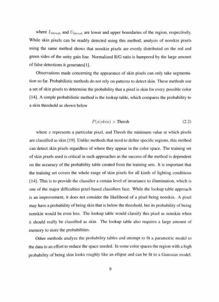
Observations made concerning the appearance of skin pixels can only take segmenta
tion so far. Probabilistic methods do not rely on patterns to detect skin. These methods use
a set of skin pixels to determine the probability that a pixel is skin for every possible color
[14]. A simple probabilistic method is the lookup table, which compares the probability to
a skin threshold as shown below
P{x\skin) > Thresh (2.2)
where x represents a particular pixel, and Thresh the minimum value at which pixels
are classified as skin [19]. Unlike methods that need to define specific regions, this method
can detect skin pixels regardless of where they appear in the color space. The training set
of skin pixels used is critical in such approaches as the success of the method is dependent
on the accuracy of the probability table created from the training sets. It is important that
the training set covers the whole range of skin pixels for all kinds of lighting conditions
[14]. This is to provide the classifier a certain level of invariance to illumination, which is
one of the major difficulties pixel-based classifiers face. While the lookup table approach
is an improvement, it does not consider the likelihood of a pixel being nonskin. A pixel
may have a probability of being skin that is below the threshold, but its probability of being
nonskin would be even less. The lookup table would classify this pixel as nonskin when
it should really be classified as skin. The lookup table also requires a large amount of
memory to store the probabilities.
Other methods analyze the probability tables and attempt to fit a parametric model to
the data in an effort to reduce the space needed. In some color spaces the region with a high
probability of being skin looks roughly like an ellipse and can be fit to a Gaussian model.
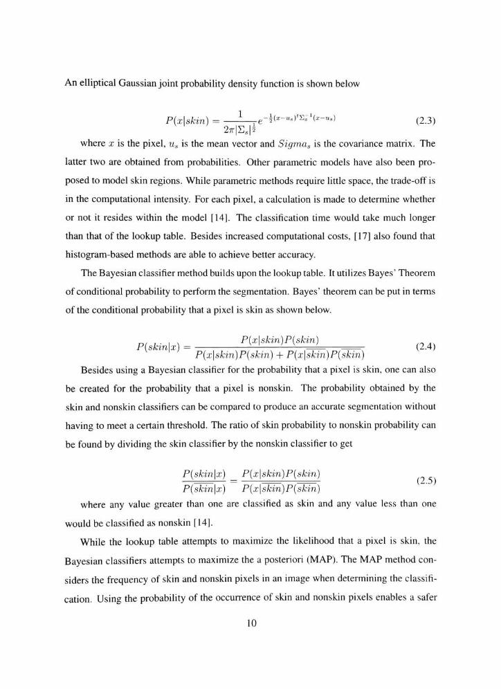
An elliptical Gaussian joint probability density function is shown below
P(x\skin) =L-^-Ks-u^sr^-t.,)
(2.3)2^|ES|2
where x is the pixel, us is the mean vector and Sigmas is the covariance matrix. The
latter two are obtained from probabilities. Other parametric models have also been pro
posed to model skin regions. While parametric methods require little space, the trade-off is
in the computational intensity. For each pixel, a calculation is made to determine whether
or not it resides within the model [14]. The classification time would take much longer
than that of the lookup table. Besides increased computational costs, [17] also found that
histogram-based methods are able to achieve better accuracy.
The Bayesian classifiermethod builds upon the lookup table. It utilizesBayes'
Theorem
of conditional probability to perform the segmentation.Bayes'
theorem can be put in terms
of the conditional probability that a pixel is skin as shown below.
.
,. . P(x\skin)P(skin) _
,x
P{skin\x) = ;' ;
\ N
-=- (2.4)P{x\skin)P{skin) + P{x\skin)P(skin)
Besides using a Bayesian classifier for the probability that a pixel is skin, one can also
be created for the probability that a pixel is nonskin. The probability obtained by the
skin and nonskin classifiers can be compared to produce an accurate segmentation without
having to meet a certain threshold. The ratio of skin probability to nonskin probability can
be found by dividing the skin classifier by the nonskin classifier to get
P{skin\x) P{x\skin)P{skin)
P{skin\x) P(x\skin)P{skin)
where any value greater than one are classified as skin and any value less than one
would be classified as nonskin [14].
While the lookup table attempts to maximize the likelihood that a pixel is skin, the
Bayesian classifiers attempts to maximize the a posteriori (MAP). The MAP method con
siders the frequency of skin and nonskin pixels in an image when determining the classifi
cation. Using the probability of the occurrence of skin and nonskin pixels enables a safer
10
classification of pixels than when their skin and nonskin probability are similar. For exam
ple, if it was calculated that 75% of the pixels in the training images were nonskin, then
given nearly equal probabilities for a pixel, there is a better chance that the pixel is nonskin.
The ML method used for the lookup table assumes P{skin) = P{skin) [19] and could not
make this adjustment.
2.2.2 Face localization
The classification of pixels as skin and nonskin is only one component of the face detector.
Feature-invariantmethods are typically bottom-up approaches. Once the classified image is
divided into skin and nonskin regions, the skin regions can be analyzed for facial features.
Features such as eyes, nose, and lips can be searched for to differentiate the faces from
hands and other skin areas. Another approach would be to look at the shape of the region
and compare it to the shape of a face. Since faces are generally elliptical in shape, each
object can be examined for elliptical-like qualities. Fitting an ellipse to an object is a
much simpler and less time consuming approach than trying to find multiple features and
analyzing their location in the image. Geometric moments could also be used to determine
the ellipse-like qualities of each object. A least square fitting algorithm for fitting ellipses
was proposed in [3] which improves upon the time needed to find the ellipse, and is used
here.
The direct least square fitting of ellipses uses an algebraic model for a conic to fit the
ellipse to the data points. The equation for a general conic is
F{a, x) = a x =ax2
+ bxy +cy2
+ dx + ey + f = 0 (2.6)
where a = [a b c d ef]T
and x =[x2
xyy2
x y 1}T. The fitting for a conic can be
accomplished by minimizing the sum of squared algebraic distances, which can be viewed
as
11

N
DAa) =J2Hxi)2
(2-7)
t-i
forN data points. Adding a quadratic constraint to the parameters allows the minimiza
tion to be solved by the following rank-deficient generalized eigenvalue problem
DTDa = Sa = XCa (2.8)
where D = [xi x2 xn}t> which is the design matrix, S = DTD is then the scatter
matrix, and C is the quadratic constraint.
A conic is elliptical if the discriminantb2
Aac < 0. Since an elliptical region is
desired, using this restriction on the discriminant as the constraint would result in an el
lipse. However, the Kuhn-Tucker conditions do not guarantee a solution for minimization
of quadratic forms that are subject to this type of non-convex inequality constraint. This
problem can be circumvented by arbitrarily scaling the parameters and include the scaling
as part of the constraint. The constraing C was chosen to be Aacb2
1.
Using the Lagrange multiplier A and differentiating, the following system of simulta
neous equations is obtained as a necessary condition for a solution to be a minimum.
Sa = XCa (2.9)
aTCa = l (2.10)
Assuming (Aj, u) solves the above equations, then so does (Aj, put) for any real scalar
p. Using the constraint equation, the value of p{ can be solved for in the constraint as
AfuJCui 1. Through substitution of the minimization equation, pt can be found to be
*=v^(2-n)
The ellipse fitting can finally be solved by setting dj = piUi. Fitzgibbon, Pilu, and
Fisher [3] go on to show through a series of proofs that there is exactly one negative gener
alized eigenvalue in the solution, and it is the elliptical solution.
12
The direct least square fitting algorithm for the ellipses discussed fits well into the
system as the equation is relatively simple, efficient, robust, and guarantees an elliptical
result. Fitzgibbon, Pilu, and Fisher [3] also claim that this method is less computationally
expensive than its predecessors.
2.3 FPGA architectures
Morphological dilation and erosion as well as the connected components algorithm were
implemented in VHDL. The rational used to select these operations is discussed in section
4.2 on page 41. Similar work in these areas is presented in this section.
2.3.1 Morphological implementations
Morphological dilation and erosion are used to expand(dilation) or contract(erosion) the
edges of objects within an image. A structuring element is used to determine how far the
edges are dilated or eroded. Further details on these operations are provided in section 3.4
on page 24 in the design section of the paper.
Ong and Sunwoo [9] investigated a cost-effective morphological filter chip. The chip
usesmultiple steps to compute themorphological result. Using dilation as an example, each
column of the image being input into the system is of course loaded into input registers.
Three pixels of the structuring element are retrieved from three circular buffers. The first
step consists of storing the results of additions in the partial results registers provided for
by the feedback loop. Comparisons are then performed as well as the detecting of the
maximum value for the dilation to be performed. The second step consists of the maximum
value being given back to the comparator and evaluated again, and the third step consists of
giving the maximum value to be stored in the partial results register and then given back to
the comparator once again; when the third step has been completed, the dilation operation
has finished and the final result is stored in the output register. After the dilation operation
has been completed, the last partial results register is cleared back to zero. Figure 2. 1 shows
13

the architecture used for implementation.
add/
subtract
P-
add/
subtract
P,
add/
subtract
TCB
o
I
P4
Feedback Loop Path
Figure 2. 1 : Morphological filter chip
This chip contains a feedback loop path to reuse partial results. This path reduces
the number of comparators and adding and subtracting units; only three adding and sub
tracting units are needed instead of the more prevalent nine. In addition, this architecture
only requires fives registers instead of eight to reuse partial results. One four-input de
coder/encoder pair comparator is also used. Three Circular Buffers are used to contain the
structuring element as well as to keep the number of pins low. Each cell of the structur
ing element is contained in three circular buffers one at a time; after all the pixels of the
structuring element are amassed, three pixels are sent to the three adding and subtracting
units. These pixels are added for dilation or subtracted for erosion with pixels of the input
image. Dilation requires nine additions and eight two-operand comparisons; however, the
feedback loop mentioned earlier can help reduce hardware units. The erosion function can
be executed in only three steps (the same as dilation); however, instead of additions and
finding maximum values, subtractions and finding minimum values are performed; there
fore, both of these operations can be executed using the same hardware, albeit the different
units used for both operations.
Ong and Sunwoo [9] concluded that their design may require less hardware and may
14
also be faster than other architectures it was compared against.
Deforges and Normand [2] presented another morphological hardware implementation
that uses a new structuring element decomposition method. The main components used in
this approach are discussed here. The first ofwhich is structuring elements. Four two-pixel
structuring elements are sufficient to construct any 8-convex element as several of both set
unions and dilations. Most of the structuring elements used are symmetrical; most can
be acquired by restricting formulas to simply elementary dilations. In this way, elements
are simple to describe since only the index element being used for the dilation need be
specified.
The second item to discuss is the systolic processor. As mentioned earlier, the algo
rithm is confining the relationship area to the 8-connected region. This makes it easy for
a specific architecture to be designed according to the same process. The process needs to
store one row of previously gained results to provide values within the region. To avoid
multiple address management caused from the specifications of the algorithm to depend on
the actual two-pixel structuring elements, some temporal relationships are created. Now, to
get values within the region, the row memory need only be accessed one time by pipelin
ing the positions in each row. A synchronous dual port ram is implemented to create a
FIFO-like memory, which allows both reading and writing to occur during a single clock
cycle.
Finally, the global architecture is discussed. A simple global control unit is of necessity
to this system; it manages the addresses as well as the signal generation at the start of each
row. The maximum extraction module implies that only a comparator and multiplexer are
needed. The systolic processor as discussed above, and which is dedicated to the dilation
by the structuring element, is also needed. Additional registers are used to pipeline the
combinatorial phases which introduce a bit of latency, but the synchronous data path is
restricted by one stage alone. Maximum clock rate is therefore dependent only on one
combinatorial phase.
15
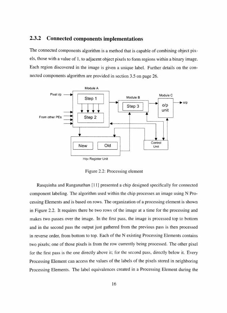
2.3.2 Connected components implementations
The connected components algorithm is a method that is capable of combining object pix
els, those with a value of 1, to adjacent object pixels to form regions within a binary image.
Each region discovered in the image is given a unique label. Further details on the con
nected components algorithm are provided in section 3.5 on page 26.
Module A
Pixel i/p Module C
From other PEs
? o/p
Hqv Register Unit
Figure 2.2: Processing element
Rasquinha and Ranganathan [11] presented a chip designed specifically for connected
component labeling. The algorithm used within the chip processes an image using N Pro
cessing Elements and is based on rows. The organization of a processing element is shown
in Figure 2.2. It requires there be two rows of the image at a time for the processing and
makes two passes over the image. In the first pass, the image is processed top to bottom
and in the second pass the output just gathered from the previous pass is then processed
in reverse order, from bottom to top. Each of the N existing Processing Elements contains
two pixels; one of those pixels is from the row currently being processed. The other pixel
for the first pass is the one directly above it; for the second pass, directly below it. Every
Processing Element can access the values of the labels of the pixels stored in neighboring
Processing Elements. The label equivalences created in a Processing Element during the
16
processing is stored within the Processing Element. Subsequently, this equivalence is sent
to other pixels in the row by left shifting them through the linear array of Processing Ele
ments. Each processor cell is organized by three main parts, which work concurrently by
pipelining and are controlled by a control unit. The architecture is designed in such a way
as to implement both passes through the image as a single unit; the Pass signal given by
the host determines the logic that is used in each Processing Element. To improve on speed
and performance, each Processing Element is designed to implement a four stage pipeline
for the first pass, and a three state pipeline for the second. The first two modules are used
to execute the first two steps of the algorithm, and the lastmodule is used for shifting labels
out and is not used for computational purposes.
Rasquinha and Ranganathan [11] performed a simulation using eight Processing Ele
ments (any number of Processing Elements can be used without any effect on throughput)
implemented on an FPGA rapid prototyping system consisting of four XC4010 FPGAs at
a frequency of about 35 MHz. The critical path could be shown to be in the second pipeline
of the firstmodule and was calculated to be 1 1 nanoseconds. Giving another 3 nanoseconds
for register delays, a total clock period of 14 nanoseconds was calculated; the chip executes
at a maximum clock frequency of 71.4 MHz and using 2 micron technology. Transferring
the architecture to a more powerful, lower micron technology should improve the speed
quite a bit.
Another approach uses parallel region labeling within a 3x4 window [18]. This ap
proach uses a label assigning block with raster scan scheme to concurrently process two
label-assigning functions for a binary image which has been input to the system. Two re
sults are achieved, the first is that it appoints the initial label, the second is that it finds the
label pair in the corresponding connected component. The processing block also merges
labels and then outputs a symbolic image.
The value of each pixel within the binary image input to the system is either a 1, an ob
ject, or a 0, part of the background. The label-assigning must therefore give an initial label
to a 1 -pixel. The 3x4 window discussed above can be used to help speed up this process
17

since the image data is given by the raster scan, because it shows that certain pixels are
adjacent to other pixels. For 1-pixels therefore, the adjacentpixels'
labels are evaluated (if
the certain pixel is a 0-pixel, its pair is simply null). At the same time, the equivalent pair is
created while the label values in pairs of surrounding pixels are different. New label values
are given for the certain pixel if there is no label value in the pixels adjacent to it. Using this
algorithm, all 1 -pixels should have been assigned labels. Additionally, in order to merge
these labels with those of a connected component, a class register array is used. When
the input label receives an equivalent pair, it has two register locations; after reading and
subsequently comparing the data of the two registers, the smaller label can be completely
replaced by the larger one. Also, in the second raster scan phase, the class register array can
be used to retrieve the final label value in order to acquire the symbolic image as discussed
in the first paragraph above, which is the output of this operation. Delving deeper into the
hardware aspect, the label-assigning block retrieves two pixel information from the binary
image memory and then appoints the interim label for each pixel to be saved into the image
memory. And, because the register array only processes one equivalent pair at a time, the
combination block is used to re-organize the two given pairs. The label image memory is
then read and evaluated by the class registry array to complete any and all label merges for
the connected component.
To conclude, this labeling architecture can be verified on an FPGA which takes 6 1 20
logic elements with a working frequency of 80 MHz, which makes this connected com
ponent labeling assignment method a faster one. The architecture uses two processing
elements and one class registry array to achieve the label assignment discussed in detail
above in two raster scans. This design therefore gives better performance; with an FPGA
implementation, real time operation can be achieved.
An overview of face detection methods, specifically focusing on feature-invariant ap
proaches using skin color and face shape were covered in this chapter. Lastly, hardware
architectures similar to the implementations presented in this work were discussed. Now
that a foundation of face detection research has been laid, the face detection method used

for this thesis will be presented.
19

Chapter 3
Design
In order to compare software and FPGA performance in face detection, a simple face detec
tor has been implemented. High-level detection methods are not suited for FPGA design,
so this detector focuses on low-level methods. This chapter provides a high-level overview
of the face detector followed by a detailed description of each component. The face detec
tor uses Bayesian classification to divide the image into skin and nonskin pixels, which are
then grouped into objects. An ellipse is fit to each object in order to compare its shape to
that of an ellipse. If the shape of the ellipse resembles that of a face and the object is a close
match to the ellipse, it is classified as a face and extracted. Figure 3.1 shows the flowchart
containing the entire face detection process.
YCrCb
conversion
; Color correctionBayesian
classification
. Gap closing Object detection
Face extraction'
Elliptical
filteringElliptical fitting > ;
2-'-
Preliminaryfiltering
Figure 3.1: Face detector flowchart
20

3.1 YCrCb conversion
Images are typically expressed in the RGB color space, however, it is a poor color space
in which to analyze a pixel's color information in. The YCrCb color space separates the
luminance information, Y, from the chrominance information, Cr and Cb, which allows
for a more accurate portrayal of the color of a pixel. Yang notes that most differences in
skin color reside in the intensity rather than the chrominance [16], so a color space that
can explicitly single this information out is beneficial. Ignoring the luminance component
significantly reduces the difference in appearance of pixels and improve our ability to ac
curately determine the pixel's type. Using the YCrCb color space gives some illumination
invariance as most of the differences in lighting are in the luminance component. The
transform from RGB to YCrCb is shown below.
Y = 0.299.R + 0.587G + 0.114E (3.1)
CR = R-Y (3.2)
CB = B-Y (3.3)
The simplicity of the transform incurs little to no overhead in the face detection process
while providing a more accurate portrayal of each pixel's color information.
3.2 Color correction
Converting to the YCrCb color space helps to minimize the affect of different lighting
conditions in images; however, it does not account for how different input devices express
color information as it is captured. Viewing the exact same scene taken at the exact same
time by two different types of cameras will appear slightly different as each camera has
slightly different hardware which interprets the scene differently. While there is no way to
get every input device to interpret a scene in the same way, there are methods to balance
the color within the image.
21

The gray-world assumption is one method used tominimize the difference. Thismethod
assumes that the average of each color component within an image is gray. If the compo
nent does not average to gray, then that component within each pixel can be scaled, so
that the component will average to gray. While this assumption is by no means perfect, it
provides a common base in which to normalize different images.
Gray-world averaging is used to normalize how the Cr and Cb components appear
in different images. Correcting the color of the image through gray-world averaging is
important so as to maintain the robustness of the classification as the location or input
device changes. Without gray-world averaging, every time one of these things is changed,
the classifier would need to be retrained else itwould subsequently suffer from a low correct
detection rate.
3.3 Bayesian classification
Once the image has been converted to the YCrCb color space and color correction has
been performed in an attempt to normalize color appearance, Bayesian classification can be
used to divide the image into skin and nonskin pixels. Bayesian classification uses a priori
knowledge of the probability a pixel is skin and nonskin based on its color information.
Using both probabilities, it is able to make a determination if the pixel is likely to be skin
or nonskin.
Bayesian classification is based onBayes'
equation. The equation determines the prob
ability that an object is a particular type given that object. When applied to skin and non
skin pixels, it would be the probability a pixel is skin or nonskin given the pixel. The actual
equation in terms of skin probability is shown below
,. P(x\skin)P(skin)
P{skin\x) = N ;' '
\ -
/
=-
(3.4)P{x\skin)P{skin) + P{x\skin)P(skin)
where x represents the pixel and P{x\skin) and P{skin) are probabilities that are
known a priori. The skin and nonskin probabilities for a given pixel can be compared by
22

applying the same equation to the pixel's nonskin probability. Combining and simplifying
the equations yield
P(x\skin)P(skin) > P{x\skin)P{skin) (3.5)
where the pixel is determined to be skin if the statement evaluates to true and nonskin if
it evaluates to false. The equation can be further simplified by combining the skin and non
skin probability values into a threshold value. This is possible since the skin and nonskin
probability values are independent of the pixel used. The final equation is shown below.
P{x\skin) > P(x\skin) thresh (3.6)
Besides simplifying the equation, the thresh value adds flexibility to the calculation.
It can be adjusted to give more weighting to the pixel's skin probability or nonskin prob
ability, which causes the equation to classify pixels as skin more aggressively or more
conservatively.
The Bayesian classification uses the color of the pixel to determine the conditional
probabilities for the pixel's type given the pixel; however, any feature of the pixel may
be used for this purpose. In order to use the pixel's color to determine the conditional
probabilities, the skin and nonskin probabilities for each possible color within the color
space need to be determined. A set of pixels predetermined to be skin or nonskin are used
to determine the probabilities. This process is referred to as training.
The actual classification iterates through the image and classifies each pixel as either
skin or nonskin based on the modified version ofBayes'
equation and the pixel's color
information. Upon completion the image is expressed in terms of skin pixels and nonskin
pixels.
23
3.4 Gap closing
The classification process makes an educated decision as to whether a pixel is skin or
nonskin; however, the classifier is basing its decision on the likelihood that a pixel is of
a particular type. While a pixel may be more likely to be one type rather than another, it
still may be of the other type. It is expected that the skin color classifier will do a good
job segmenting the image, but not a perfect job. As a result, there will be holes and gaps
within the areas classified as skin. Patching these gaps will give the face detector a more
accurate depiction of the skin areas within the image. One way to close these gaps would
be morphological closing.
The morphological closing operation is an image processing technique to fill in holes
within an object while maintaining the appearance of the rest of the image. The operation
is actually a combination of image dilation and image erosion. Image dilation expands all
the edges within the image based on the shape of the structuring block. The structuring
block is further discussed below. In this case, the goal of dilation is to fill in the areas
within the objects. After the dilation is completed, erosion is used to cause all of the edges
in the image to recede based on the shape of its structuring block. The erosion process is
the opposite of the dilation process, and causes all the object edges within the image to
recede to where they existed before dilation, however, the areas within the object should no
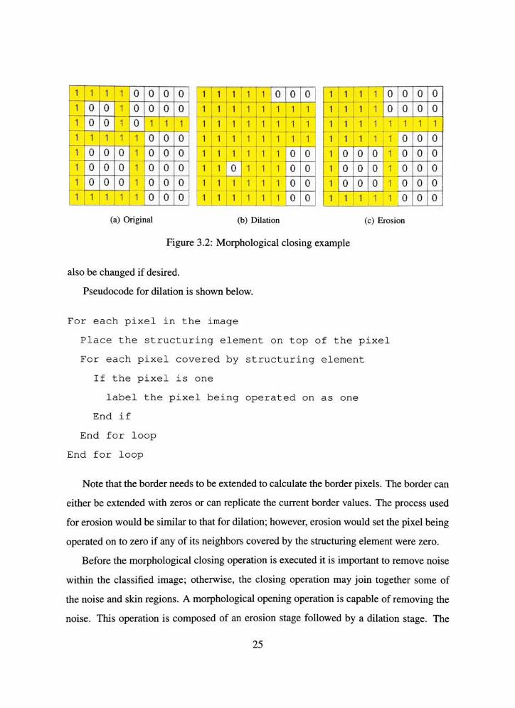
longer have edges and remain untouched. An example of this process using a 3x3 square
structuring element is shown in Figure 3.2. The first pane shows the original image, while
the next pane depicts the image after dilation. Notice how the top hole is completely filled
in while the bottom one still contains an edge. The final pane shows the image after the
erosion stage. It can be seen how the top hole was not affected but the bottom hole, which
still had an edge, now appears as it originally did.
The structuring block determines the area that is used to determine if a pixel should
be dilated or eroded. The structuring block is placed upon the pixel, and the other pixels
which it covers are used to determine the result of the operation. Thus, a larger structuring
block considers more pixels than a smaller structuring block. The shape of the block can
24
1 1i1 1 0 0 0 0
1 0 0 1 0 0 0 0
1 0 0 1 0 1 1 1
1 1 i 1 1 1 j 0 0 0
1 0 0 0 1 0 0 0
1 0 0 0 1|0 0 0
1 0 0 0 1 0 0 0
1 1 1 1 1 0 0 0
1 1 1:0 0 0
1 1 1 i 1 1 1
1 1 1 1 1 1
1 1 1 1 1 1 1
1 1 1 10 o !
1 0 1 1(0 o
1 1 1 1 jo 0
1 1 1 1 0 0
1 j 1 | 1 | 0 0 0 0
1 0 0 0
1 I 1 1 1 1 1 1
1 1 1 1 0 0 0
0 0 0 1 |0 0 0
T 0 0 1 so 0 0
0 0 0 10 0 0
1 1 1 1 1 |o 0 0
(a) Original (b) Dilation
Figure 3.2: Morphological closing example
(c) Erosion
also be changed if desired.
Pseudocode for dilation is shown below.
For each pixel in the image
Place the structuring element on top of the pixel
For each pixel covered by structuring element
If the pixel is one
label the pixel being operated on as one
End if
End for loop
End for loop
Note that the border needs to be extended to calculate the border pixels. The border can
either be extended with zeros or can replicate the current border values. The process used
for erosion would be similar to that for dilation; however, erosion would set the pixel being
operated on to zero if any of its neighbors covered by the structuring element were zero.
Before the morphological closing operation is executed it is important to remove noise
within the classified image; otherwise, the closing operation may join together some of
the noise and skin regions. A morphological opening operation is capable of removing the
noise. This operation is composed of an erosion stage followed by a dilation stage. The
25
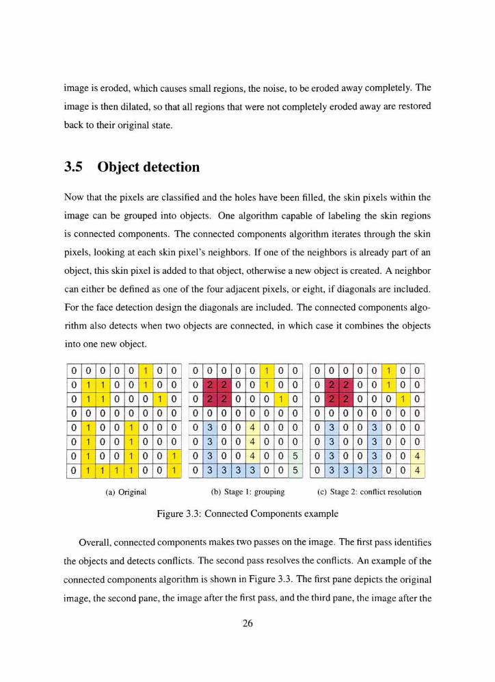
image is eroded, which causes small regions, the noise, to be eroded away completely. The
image is then dilated, so that all regions that were not completely eroded away are restored
back to their original state.
3.5 Object detection
Now that the pixels are classified and the holes have been filled, the skin pixels within the
image can be grouped into objects. One algorithm capable of labeling the skin regions
is connected components. The connected components algorithm iterates through the skin
pixels, looking at each skin pixel's neighbors. If one of the neighbors is already part of an
object, this skin pixel is added to that object, otherwise a new object is created. A neighbor
can either be defined as one of the four adjacent pixels, or eight, if diagonals are included.
For the face detection design the diagonals are included. The connected components algo
rithm also detects when two objects are connected, in which case it combines the objects
into one new object.
0 0 0 0 0 1 0 0
0 1 1 0 0 1 0 0
0 1 1 0 0 0 1 0
0 0 0 0 0 0 0 0
0 1 0 0 1 0 0 !0 1 0 0 1 0 0 0
0 1 0 0 1 0 0 1
0 1 1 1 1 0 0 1
0 0 0 0 0 1 0 0
2 0 0 1 jo 0
0 2 JO 0 0 1 jo
0 0 0 0 0 0 0 0
0 3 JO 0 4 |0 0 o j
0 3 0 o 4 JO 0 0
0 3 0 0 4 0 0 5 !
0 3 3 3 3 ;0 0 5 |
0 0 0 0 0 1 : 0 0
2 2 0 0 1 p 0
o 2|2 0 0 p 1 iO
0 0 | 0 0 o|o 0 0
0 3 0 0 3 ; 0 0 0
0 3 0 0 3 0 0 0
0 3 j 0 0 3 p 0 4
0 3 3 3 3 0 0 4;
(a) Original (b) Stage 1: grouping (c) Stage 2: conflict resolution
Figure 3.3: Connected Components example
Overall, connected components makes two passes on the image. The first pass identifies
the objects and detects conflicts. The second pass resolves the conflicts. An example of the
connected components algorithm is shown in Figure 3.3. The first pane depicts the original
image, the second pane, the image after the first pass, and the third pane, the image after the
26

second pass. Note that the objects that came in contact in the second pane were combined
into one object in the third pane.
Pseudocode for the connected components algorithm is below.
Pass 1:
For each skin pixel
For each neighbor of the skin pixel
If neighbor is part of an object
If current pixel is not part of an object
Add current pixel to this object
Else
Add entry to conflict list for these two objects
End if
End if
End for loop
If current pixel is not part of an object
Create a new object and add current pixel
End if
End for loop
Pass 2:
For each skin pixel
If skin pixel's object is in the conflict list
Change pixel's value to conflict resolved value
End if
End for loop
Additionally the object values can be updated so that they are sequential, as demon
strated in Figure 3.3.
27

Once the skin regions are identified as objects, higher level analysis can be performed
on these regions, which will now be called face candidates, to separate the faces from other
skin regions.
3.6 Preliminary filtering
The next three stages comprise the high-level filtering of the image. The preliminary fil
tering step removes any candidates that are definitely not faces. There is no need to waste
additional computation time on these objects. In this stage the shape and size of the can
didate are analyzed. If the candidate is too small to be a face that would be of interest, the
object is removed. Also, any object whose ratio of width and length is too large will be
removed.
3.7 Elliptical fitting
The primary feature used to separate faces from other skin regions is the shape of the region.
If the region is a face, then it will have an elliptical-like shape. Of course, this method is
hampered by facial hair and other things that obscure the face, but should be sufficient to
obtain a rough idea of performance.
In order to compare the candidates to ellipses, ellipses need to be fit to each candidate.
The elliptical fitting method proposed by [3] was used for this purpose. Detailed informa
tion about the method can be found in section 2.2.2 on page 11. The method fits an ellipse
to the outline of an object, regardless of the shape.
Before an ellipse is fit to the candidate, the outline of the region needs to be extracted.
The erosion operation previously discussed is used to remove the edge of the candidate.
The candidate is then subtracted from its eroded version to obtain the outline, which was
the edge that was removed.
A general conic equation is obtained after performing the elliptical fitting. This is
28
converted to an ellipse-specific equation.
3.8 Elliptical filtering
The elliptical fitting method will fit ellipses to all candidates, so the shape of the ellipse
must be compared to the shape of the actual candidate to determine how well it fit. For
each pixel that is part of the face candidate, it is determined if the pixel falls within the
ellipse or not. The number of pixels that are within the ellipse are compared to the area of
the ellipse. The candidate is removed if sufficient area within the ellipse is not covered.
The shape of the ellipse is also analyzed in a similar way that the original shape was
in preliminary filtering. If the width to height ratio is too large, then the candidate is also
removed.
3.9 Face extraction
The candidates that pass the filtering process are considered to be faces; they will be ex
tracted from the original image as detected faces. A rectangular region with the width,
height, and orientation of the ellipse fit to the face is used as a boundary for the region to
be extracted.
The face detection method covered in this chapter contains many components. The
components were implemented inMatlab, C++, and on an FPGA using VHDL. The details
of these implementations are presented in the next chapter.
29

Chapter 4
Implementation
The face detector was implemented in both software and hardware in order to compare their
performance. The software implementation was first written inMatlab for prototyping and
then in C++ for optimal performance. Analysis of the C++ implementation showed which
components were most time consuming. Those were implemented in VHDL in order to
obtain a good estimate of a hardware version of the face detector. The details of these
implementations are discussed in this chapter.
4.1 Software
The software implementations in Matlab and C++ were conceptually the same, although
the structure of each program was slightly different. Any significant differences between
the implementations is noted throughout this section. This section first covers the general
implementation and then the structure of both the Matlab and C++ versions.
4.1.1 YCrCb conversion
The conversion from RGB to YCrCb was straightforward. A loop was created to iterate
through the input pixels and convert each pixel to the YCrCb color space. The result was
stored within a new image.
30
4.1.2 Color correction
The color correction component first determines a correction value for each component
in the color space, and then applies those corrections to each pixel in the image. The
correction for each color component is the average value of that component in the image
subtracted from its gray level value. In the case of the YCrCb color space, the gray level
value for both chrominance components is zero, while the Cr and Cb ranges are from 179
to 179 and 226 to 226 respectively. Once the correction values are determined, they are
applied to their respective components. If the correction causes the component's value to
exceed its range, then the value is set to the range's limit.
4.1.3 Bayesian classification
The pixel classification component used the Bayesian classifier equation to classify compo
nents. The parameters for the script are a skin probability map, a nonskin probability map,
and a threshold value. The classifier's flexibility allowed for different probability maps and
threshold weights to be analyzed without any modifications.
4.1.4 Gap closing
The morphological opening and closing operations used 3x3 structuring elements to pro
cess the image. A larger structuring element was not chosen so as to prevent the mor
phological closing operation from joining two separate skin regions. The implementation
of the dilation and erosion methods are built into the Matlab libraries, however they were
implemented following the algorithm detailed in section 3.4 on page 24 for the C++ face
detector.
31
4.1.5 Object detection
The implementation of the connected components algorithm follows the pseudocode de
scribed in section 3.5 on page 26. The connected components algorithm starts in the upper-
left corner of the image and works across the rows until the bottom-right corner is reached.
Since only the pixels already processed have been assigned to an object, only the neighbors
of a pixel that have been processed will be analyzed in determining the value of the current
pixel. This would include the pixels in the row above the current pixel and the pixel just to
the left of the current pixel.
The pseudocode did not explain how to implement the conflict handling. The conflicts
were handled through use of a conflict table that maps a pixel's object value to the new
value after conflicts have been resolved. The table is updated each time a new object is
added or a conflict is detected in order to keep the table and algorithm in sync. The table
also needs to keep track of the number of conflicts. The pseudocode for adding a new
object is shown below.
Add a new entry table [newObj ]
Set the entry value to newObj-
numConflicts
Note that the object's initial value is determined by subtracting the number of conflicts
already detected. This is to keep the table continuous. Each time a conflict is resolved,
one object value is no longer used; however, by decrementing each subsequent object by
one, it can be replaced. New objects are decremented by the number of conflicts to account
for these lost objects. More details on resolving conflicts can be found in the following
pseudocode.
If table [objl] != table[obj2]
numConflicts= numConflicts + 1
If table [objl] > table [obj2]
higher = table [objl]
lower = table [obj2]
32

Else
higher = table [obj2]
lower = table [objl]
End if
For lower to tableSize
If table [val] == higher
table [val] = lower
Else If table [val] > higher
table [val] = table [val]- 1
End if
End for loop
End if
When resolving a conflict, the conflct table first checks to see if this is a new conflict.
If so, the object with a higher value is merged into the object with the lower value. As
mentioned above, subsequent objects are decremeted by one to keep the known regions
sequential.
The second pass of the connected components is basically just looking up the conflict
resolved value for each pixel. However, additional computation was added to the second
pass in order to speed up the preliminary filtering stage. The filtering stage uses the height,
width, and area of each object detected in this stage. Since each pixel is already being
accessed for the second pass, the information needed for each object is also calculated.
4.1.6 Preliminary filtering
The preliminary filtering component filters objects based on size and height to width ratio.
In order for a region to be a face candidate, its area must be at least one percent of the
total image area, and a maximum 2:1 ratio between height and width. The size restriction
removes skin regions of a trivial size. The height to width ratio restriction removes skin
regions that do not have dimensions that would be expected of a facial region.
33

4.1.7 Elliptical fitting
The elliptical fitting stage uses erosion to extract the edge of the object as described in
section 3.4 on page 24. The erosion operation implemented for gap closing was modified so
that a specific value within the image could be eroded. The operation looks for pixels with
that value and erodes them if all their neighboring pixels covered by the 3x3 structuring
element do not also have that value. The enhanced erosion technique was only used in the
C++ implementation as erosion is built into Matlab. In the case ofMatlab, the image is
compared to the desired object value, which returns a new image comprised of ones, where
the pixel matched the object value, and zeroes throughout the rest of the image. This new
image could be used withMatlab's erosion function.
The elliptical fitting method described in section 2.2.2 on page 1 1 was implemented
and used for this stage. Source code provided by Fitzgibbon, Pilu, and Fisher [3] was
incorportated into the Matlab implementation. The elliptical fitting code as well as the
Matlab functions used within the code were ported to the C++ implementation.
4.1.8 Elliptical filtering
Once an ellipse is fitted to a face candidate, the shape of the ellipse and how well the object
matches the ellipse are analyzed to separate out the perceived faces. Like the height to
width ratio restrictions for the preliminary filtering, the major and minor axes of the ellipse
must maintain a 2:1 or less ratio to be considered a face.
If the ratio of the major and minor axes are within the acceptable range, the shape of
the object and ellipse are compared. Since it is guaranteed that an ellipse will be fit to each
object, it is necessary to see how well it fit in order to determine if this is a face region. The
number of pixels within the object that reside within or on the ellipse are added together.
This value is compared to the total area of the ellipse. A face candidate must fill at least
75% of the elliptical area to be deemed a face. The percentage used for the area requirement
was determined through testing.
34

4.1.9 Face extraction
The face extraction stage extracts a rectangular region from the image containing the face.
The width of the image is the length of the minor axis and the height is the length of the
major axis. Each pixel within this region is extracted and added to a new image. If the
subject's head is tilted, the orientation is corrected so that the head appears upright in the
image. The tilt correction assumes that the subject's head is no more than 90 degrees from
being upright. Finally, each face extracted is written to a file.
4.1.10 Training the classifier
The Bayesian classifier relies on the skin and nonskin conditional probabilities known for
every color within the color space. These probabilities are determined through use of the
color information for a set of pixels already known to be skin and nonskin. These pixels
are used in the creation of a training set. The accuracy of the classifier relies upon the data
within the training set, therefore it is critical to create a robust training set.
The training set is composed of a group of images containing a variety of faces with
varying skin tone, facial expressions, orientation, fighting, and backgrounds. Various re
search teams have spent time developing training sets for this purpose. Many of these sets
are made available freely to the academic community.
Originally the Aleix database created at Purdue University [8] was chosen to train the
Bayesian classifier. However, the database used a white background for each image. Since
the background of an image affects how the input device interprets the rest of the image, the
database was unable to robustly represent various ways skin color appears, and could not
be used. The Color FERET image library created by NIST[10] was chosen to replace the
Aleix database. The Color FERET database is extremely large and provides images taken
with various backgrounds, fighting sources, and skin tones among many other variations,
and which provides a robust set of pixels in which to train the classifier. NIST's release
agreement prohibits sample images from being included, so no images are provided.
35
Two hundred and fifty frontal poses were selected from the database to be used as the
training set. In order for these training images to be useful, the skin and nonskin regions
need to be identified as skin and nonskin. Once the regions are known, probability tables
can be created for both skin and nonskin. The creation of the probability tables is discussed
later. A mapping image was created for each image in the training set. Each mapping image
was created with the same dimensions as its training image. Each pixel in the mapping im
age is either black, green, or blue. Green pixels represent skin pixels, blue pixels represent
clothing, hair, eyes, eyebrows, lips, and nostrils, while black represents everything else.
The green pixels are be used for training the skin probabilities and blue for the nonskin
probabilities. While the Color FERET database images have various backgrounds, there
are not enough variations for them to be included with the nonskin pixels. An example
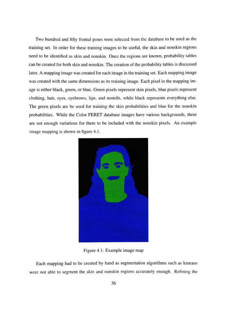
image mapping is shown in figure 4. 1 .
Figure 4.1: Example image map
Each mapping had to be created by hand as segmentation algorithms such as kmeans
were not able to segment the skin and nonskin regions accurately enough. Refining the
36

images initially segmented by such algorithms proved to be as time consuming as creating
the mappings from scratch. Adobe Photoshop and The Gimp photo editing tools were
used instead to create the image mappings. Images mappings were created over-top of the
original images using following the steps.
Select the eyes, nostrils, lips, and eyebrows using the lasso tool
Fill those areas in with blue
Draw along the outline of the face using the pencil tool in green
Select the interior of the outline using the magic wand tool
Fill in that area as green
Outline the hair and the clothing with the pencil tool in blue
Select each region with the magic wand tool and fill it in as blue
A Matlab script was also written to touch-up the mappings to fill in tiny gaps that were
not noticeable. The script filled the gaps between skin and nonskin regions as blue and then
set any pixel that was not blue or green to black, so that it would be ignored during training.
Once the mappings were created for each training image, the images could be used
to train the classifier. A two dimensional histogram representing all Cr and Cb values
was created for both skin and nonskin. The pixels from the training images were first
converted to the YCrCb color space and then color corrected using the same method as
the face detector. Each pixel in the color corrected training image was compared to the
corresponding pixel in its mapping. Pixels mapped to a green pixel were added to the skin
histogram and pixels mapped to a blue pixel were added to the nonskin histogram. When
all of the training pixels were added to the histograms, each histogram was divided by the
number of pixels within the histogram to obtain the probabilities of each. Finally a 3x3
averaging filter was used on each set of probabilities to smooth out any abnormalities in the
map.
37
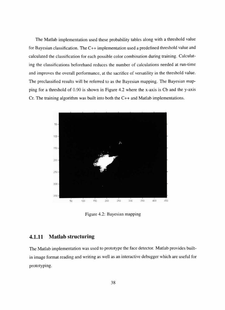
The Matlab implementation used these probability tables along with a threshold value
forBayesian classification. The C++ implementation used a predefined threshold value and
calculated the classification for each possible color combination during training. Calculat
ing the classifications beforehand reduces the number of calculations needed at run-time
and improves the overall performance, at the sacrifice of versatility in the threshold value.
The preclassified results will be referred to as the Bayesian mapping. The Bayesian map
ping for a threshold of 0.90 is shown in Figure 4.2 where the x-axis is Cb and the y-axis
Cr. The training algorithm was built into both the C++ andMatlab implementations.
50 100 150 200 250 300 350 400 -450
Figure 4.2: Bayesian mapping
4.1.11 Matlab structuring
TheMatlab implementation was used to prototype the face detector. Matlab provides built-
in image format reading and writing as well as an interactive debugger which are useful for
prototyping.
38
The Matlab code was split into four basic categories. The first category was image
segmentation, which handled any processing needed to convert images to the proper size
or format, as well as handling the image mappings. The skin classification category con
tained the scripts used for creation of the Bayesian mapping as well as the classifier itself.
This category also included the color space transform and color correction code. The next
category was object detection, which included the gap filling, connected components, and
preliminary filtering. The final category was ellipse fitting, which held the ellipse fitting
algorithms, ellipse filtering, and face extraction.
A final script was written to handle the interactions between the different groups of
scripts that connected the overall face detection implementation. The scripts were split
up into categories, so that each area of face detection could be analyzed and tested inde
pendently. Besides the code written to create the Bayesian mapping and to perform face
detection, additional scripts were written to measure the accuracy of the Bayesian classifier
as well as the entire system.
Uncompressed TIFF images were used for the creation of the Bayesian mapping and
the face detection; however, the face detection script could be modified to use any type of
image format supported by Matlab.
4.1.12 C++ structuring
C++ was used for the performance benchmarking of the software-based face detection.
C++ is compiled to machine code, which gives it a speed advantage over interpreted lan
guages such as the language used withMatlab.
The face detector is split into four files: FaceDetector.h, FaceDetector.cpp, Matrix.h,
and Image.h. FaceDetector.h and FaceDetector.cpp contain the the actual face detection
implementation while Matrix.h and Image.h are helper classes. Matrix.h contains a tem
plate class designed as a container formatrices and the matrix functionality needed for face
detection. Image.h also contains a template class. This class was designed to contain im
ages and some basic imaging operations. The helper classes were written as templates, so
39

that regardless of the data type used within the matrix or image, only one implementation
was needed. A UML diagram detailing the C++ face detection implementation is shown in
Figure 4.3.
FaceDetector
-main()
HtetectFacesO
+createMap()
-classifi'lmagef I
-fillGapsO
-fmdObjedsO
-(SterObJeolsO
-exttactFaeeO
-convertYCcCbf)
correctColort)
lilElipps<Hl
wsadlmageO
lmageT>
rows: int
cols : in!
(Sms ; Inl
data
?operator*!)
?operaior(X)
?operator+O
-^ toparator-O
+gelRowsO
?getCoteO
+gelDirns()?OHiDa;ai;
?setDataO
tadd()
?subirartO
+dil8leQ
mrodeQ
Matriy<T>
rows in!
cols : Int
*perator={)
?operatorOO
?opefator+O
?opefator-0
*operator*Q
?getCotsf)
?addf)
+sobtrac%'i
?multiplyO
HransposeQ?inverssO
?choteskyO
?jacobiO
?resizeO
priroQ
Figure 4.3: Face Detector UML Diagram
The face detector has a main function capable of creating a Bayesian mapping and
executing the face detection algorithm. The face detector class may also be included in
another C++ program where its face detection and Bayesian map creation functions can be
called directly.
A custom image format was designed for use with the face detector when it is used as
a stand-alone application. The format consists of a 16 byte header followed by the image
40

data written in binary. The header is composed of the following four 4 byte values: rows,
columns, dimensions, and bytes per dimension.
4.2 Hardware
It was not necessary to implement the entire face detection design in VHDL in order to get
a accurate estimate ofperformance. Implementing the bottlenecks within the face detection
process is sufficient. A functional break-down of the C++ face detector's execution time
was analyzed to locate the time intensive functionality. The break-down was created using
images of size 252x378 pixels. It can be found in in Figure 6.4 on page 64.
The erosion and dilation operations account for about 34% of the execution time.
These operations are pixel independent and could be significantly improved with a par
allel hardware design, and therefore a hardware design was implemented. The conversion
to YCrCb and image subtraction functionality are also pixel independent, and their perfor
mance would be close to the performance of the erosion and dilation operations. As such,
they will have similar performance and can be accurately measured by the erosion and
dilation execution time. The color correction functionality makes two passes on the im
age. The first pass finds the correction values, and the second applies the correction. Both
passes would again be similar in performance to erosion and dilation, as within a pass the
output of one pixel does not depend on another. The color correction execution time can be
computed as close to twice that of erosion or dilation. Finally, the connected components
algorithm accounts for about 13% of the execution time. This functionality is unlike the
others mentioned above, as each pixel relies on the output of the pixels processed before
it. Such an algorithm is not ideal for use in hardware, but will give an accurate estimate of
the type of performance such an algorithm should expect to have in an FPGA. Combined,
these functions account for roughly 92% of the execution time within software. If the func
tionality that makes up the remaining 8% of execution time is assumed to be at least as fast
in hardware as in software, then the performance of a complete hardware implementation
41
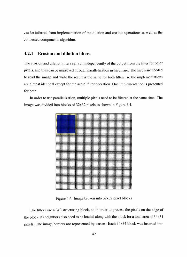
can be inferred from implementation of the dilation and erosion operations as well as the
connected components algorithm.
4.2.1 Erosion and dilation filters
The erosion and dilation filters can run independently of the output from the filter for other
pixels, and thus can be improved through parallelization in hardware. The hardware needed
to read the image and write the result is the same for both filters, so the implementations
are almost identical except for the actual filter operation. One implementation is presented
for both.
In order to use parallelization, multiple pixels need to be filtered at the same time. The
image was divided into blocks of 32x32 pixels as shown in Figure 4.4.
:"::::::::: "::::: i "in ii
IZZ'.'ZZZ'.'.'.'.'.'.l'.'.Z'. '.'.'.". '.II'.'. '.'.lll'.'.'.'.Zl'.lll'. I
:::::::::::::::::::: : ::::::::::::::: :::::::::
Figure 4.4: Image broken into 32x32 pixel blocks
The filters use a 3x3 structuring block, so in order to process the pixels on the edge of
the block, its neighbors also need to be loaded along with the block for a total area of 34x34
pixels. The image borders are represented by zeroes. Each 34x34 block was inserted into
42
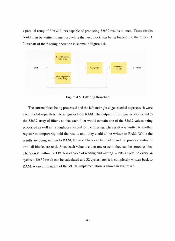
a parallel array of 32x32 filters capable of producing 32x32 results at once. These results
could then be written to memory while the next block was being loaded into the filters. A
flowchart of the filtering operation is shown in Figure 4.5.
Load block into
filler array
Apply filterStore filter
results
Load edges Into
filler array
Figure 4.5: Filtering flowchart
The current block being processed and the left and right edges needed to process it were
each loaded separately into a register from RAM. The output of this register was routed to
the 32x32 array of filters, so that each filter would contain one of the 32x32 values being
processed as well as its neighbors needed for the filtering. The result was written to another
register to temporarily hold the results until they could all be written to RAM. While the
results are being written to RAM, the next block can be read in and the process continues
until all blocks are read. Since each value is either one or zero, they can be stored as bits.
The SRAM within the FPGA is capable of reading and writing 32 bits a cycle, so every 34
cycles a 32x32 result can be calculated and 32 cycles later it is completely written back to
RAM. A circuit diagram of the VHDL implementation is shown in Figure 4.6.
43
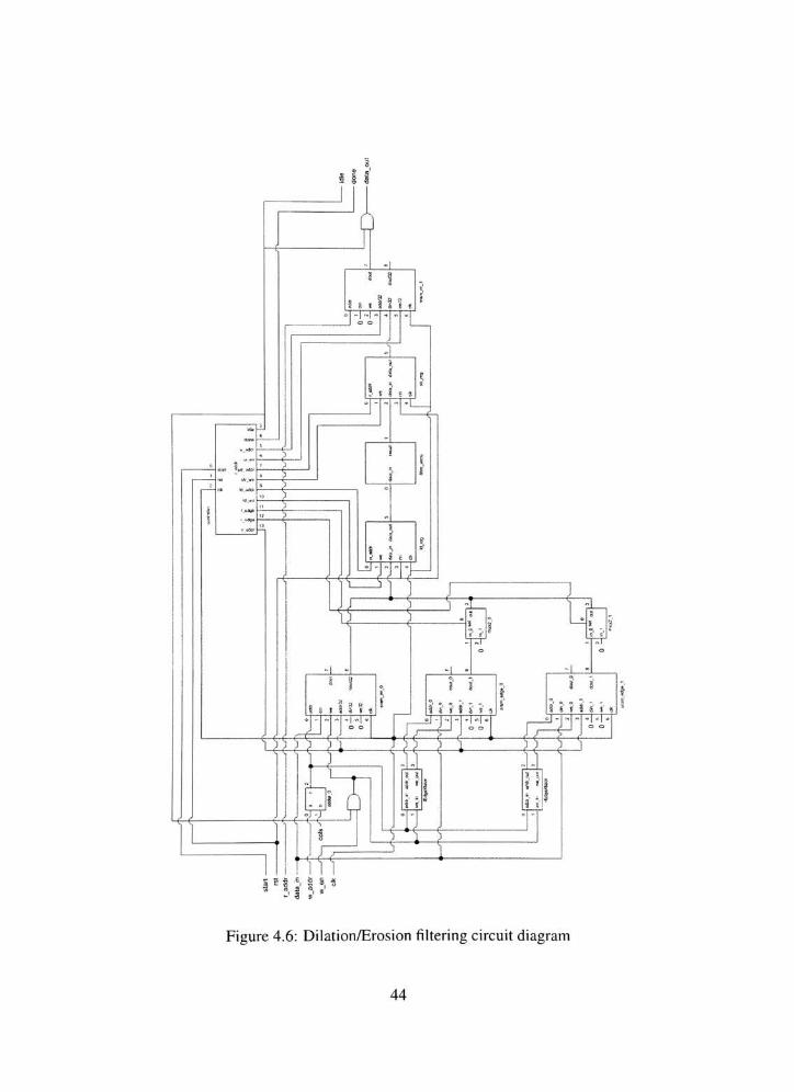
Figure 4.6: Dilation/Erosion filtering circuit diagram
44
A simple interface was implemented for reading and writing into the filtering imple
mentation. One value is written into the filtering circuit at a time. Once the start line is set
to high, the filtering process begins. When the filter is finished, the done line is set high and
the filtered data can be written out one value at a time. A more complex IO design could
have been used; however, it is only implemented to allow a testbench to load in and retrieve
data from the filter. Only the performance of the actual filtering circuit was measured.
The filter first writes the data written into the filter into three separate SRAMs. One
SRAM holds all the image data, while the other two hold the edges needed by each block.
Translators were written to detect which input values are left or right edges and to translate
their addresses into the addresses of the 32-bit row it is an edge of. Once all the data is
written, the filter can now calculate all filtering results. Each cycle one row of 32 bits is
read from the SRAM that holds the image data, and the left and right edges for that row
are also read from their respective SRAMS. If the left or right edge falls on the border of
the image, then zero is used for the edge value. These 34 bits are combined and stored
within the load register. Once all 34 rows are read into the load register, the filtering is
performed and the result is stored in the store register. The filtered values are read out of
the store register a row at a time and written into the SRAM that holds the result. The
process continues until all the pixels within the image have been processed.
The filter is divided into a three stage pipeline, so that each portion of the hardware
could be used at once. The first stage of the pipeline reads the values out of the SRAM to
filter. At the beginning of the next cycle those values are retrieved from the SRAM and can
be written into the load register, which is the beginning of the second stage of the pipeline.
The filter array and the store register are also used in the second stage. The final stage
writes the filtered results retrieved from the store register.
This implementation uses an image size of 256x384 for processing, which is approx
imately the same size as used in the software implementation's analysis. The size was
slightly extended, so that the image columns and rowscould be analyzed in 32 pixel incre
ments. Smaller images may be used by zero extending the rows to 384 pixels.
45
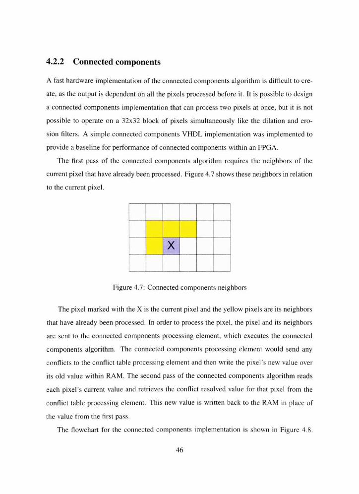
4.2.2 Connected components
A fast hardware implementation of the connected components algorithm is difficult to cre
ate, as the output is dependent on all the pixels processed before it. It is possible to design
a connected components implementation that can process two pixels at once, but it is not
possible to operate on a 32x32 block of pixels simultaneously like the dilation and ero
sion filters. A simple connected components VHDL implementation was implemented to
provide a baseline for performance of connected components within an FPGA.
The first pass of the connected components algorithm requires the neighbors of the
current pixel that have already been processed. Figure 4.7 shows these neighbors in relation
to the current pixel.
X
Figure 4.7: Connected components neighbors
The pixel marked with the X is the current pixel and the yellow pixels are its neighbors
that have already been processed. In order to process the pixel, the pixel and its neighbors
are sent to the connected components processing element, which executes the connected
components algorithm. The connected components processing element would send any
conflicts to the conflict table processing element and then write the pixel's new value over
its old value within RAM. The second pass of the connected components algorithm reads
each pixel's current value and retrieves the conflict resolved value for that pixel from the
conflict table processing element. This new value is written back to the RAM in place of
the value from the first pass.
The flowchart for the connected components implementation is shown in Figure 4.8.
46

Pass 1
Shift next column
into register
Run connected
components on
register
Add object
Resolve conflicts
Pass 2
Lookup resolved
object value
Figure 4.8: Connected components flowchart
A 2x3 window is used in the connected components processing element that contains the
neighbors needed to operate on the current pixel. Once the pixel is processed, the next two
values from the following column are read into the window and the next pixel is processed.
The output of each processed pixel is written back to RAM. If the pixel is the start of a new
object, the conflict table is updated and the new value is written back to RAM. However,
if any conflicts are detected, the circuit stalls while the conflict table processing element
resolves the conflict and then writes the new value to RAM. The left and right edges of
the image present special cases that are handled slightly differently. Once the last pixel
on a row is read and the connected components algorithm has been executed on the pixel
before it, zeroes are read in to represent the right edge and then the last pixel is operated on.
The circuit then wraps around to the first pixel in the next row. The zeroes previously read
in are now considered the left edge. The first set of pixels are read in and the connected
components processing element waits until the next set of pixels are read in to obtain the
final neighbor needed to operate on the first pixel in this row.
47

The conflict table processing element was implemented in the same way as the software
version of the conflict table was implemented. The conflict table is attached to another
portion of RAM where it stores the current value for each object. Finally, on the second
pass the conflicts have already been resolved, so the pixels within the image simply need to
be updated with their conflict resolved value. Pixels are loaded and their value is passed into
the conflict table processing element one at a time. The conflict table processing element
finds the conflict resolved value and that value is written back to RAM.
A circuit diagram of the VHDL implementation of connected components is shown in
Figure 4.9. The IO interface of the connected components implementation is similar to that
of the dilation and erosion implementations. The data is written one 1-bit value at a time
into SRAM. Once the image data is written into the connected components circuit, the start
line is set high and the first pass of the algorithm begins. Upon completion of the first pass,
the second pass begins. When the second pass finishes, the circuit sets it's done line to high,
signaling that the processing is complete. The result can then be read out one 8-bit value
at a time. The connected components implementation restricts the total number of objects
to 255, which is the same restriction used in the software implementation. Internally, 9 bits
are used to represent each image to allow for additional objects before all the conflicts are
resolved.
48
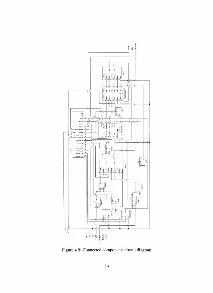
* I -8
n
i e
3
J
5 5
I
s 2 8
=5
3
S 3
tTTTTi
TT
S ? f, 45 s s,
Figure 4.9: Connected components circuit diagram
49

During the first pass, a counter is used to keep track of the current address being read
out of SRAM. Internally, the image is offset by the size of a row within memory to create a
border of zero at the top of the image, so the size of a row needs to be added to the counter
value in order to have the counter correspond to a pixel within memory. However, during
the first cycle the offset is not added so that the pixel in the preceding row can be read. The
second cycle adds the offset and reads the current pixel. Once the two values have been
read, the connected components processing element processes the previous value. If the
pixel is the start of a new object, the conflict table processing element is told about the new
object and operation continues to the next pixel. Otherwise, if any conflicts are detected, the
connected components processing element tells the system to wait and instructs the conflict
table processing element to resolve the conflict. The conflict table processing element
responds to the connected components processing element by setting its done line to high.
If another conflict needs to be resolved, the process will be repeated. The conflict table's
control line is configured by the connected components processing element to inform the
table if a new value needs to be added or if a conflict is present. Finally, the new pixel
value is written back in place of the old pixel value. Another counter is used to maintain
the current pixel that should be written to. The counters are then updated to the next pixel
value. The second pass also uses the read counter to read the current pixel. Once the pixel
is read, it bypasses the connected components processing element and obtains the conflict
resolved value directly from the conflict table using the current pixel value as an index into
the conflict table. The new value is then written back to the address pointed to by the write
counter. Both counters are then updated to process the next value.
Pipelining was also used to speed up the execution of the connected components VHDL
implementation. Three stages were used within the pipeline; the first stage controls the read
counter and which offset to use in order to read a value out of SRAM. The second stage
controls the connected components and conflict table processing elements. The final stage
controls the write counter and writing to the SRAM. The pipeline allows for the next pixel
to be read from RAM while the current pixel is being processed.
50

The connected components VHDL implementation was designed for images 252x378
pixels in size, which corresponds with the size used in analysis of the software implementa
tion's performance. Smaller images may be used by zero extending the rows to 384 pixels.
The implementations discussed in this chapter were tested to verify their functionality.
Test images were created to test the components of each implementation when possible.
Visual inspection and sample input were also used in the testing process. The complete
testing procedure is presented in the next chapter.
51

Chapter 5
Testing
The testing performed for theMatlab, C++, and VHDL implementations of the face detec
tor are presented within this chapter.
5.1 Matlab testing
The Matlab implementation was used for prototyping the face detector. As such, the valid
ity of each component needed to be tested as well as that of the complete system. A brief
explanation of how each component was tested is explained within this section. Testing of
the complete face detection system is also described.
A small set ofRGB pixels were used as input to test the YCrCb conversion. The YCrCb
value for each pixel was calculated by hand for verification against theMatlab result. RGB
values that would test the lower bound and upper bound of each value were included in the
set to make sure these conditions were being handled correctly.
A sample image was used to verify color correction. The image was converted to
YCrCb. The average Cr and Cb values were calculated and stored. The converted im
age was then used as input into the color correction script. The average Cr and Cb values
for the output were calculated and verified to be equivalent to the gray level average for
these values. Finally, the image's Cr and Cb values from before color correction were sub
tracted from the values after color correction to verify that the correction was uniformly
distributed throughout the image.
52

Preliminarily the Bayesian classifier was tested by using different values near the skin/nonskin
threshold and by verifying that these values were classified to the appropriate type. The
mapping was also tested by creating an image with every Cr and Cb combination included.
The Cr and Cb combinations were arranged to match how they are arranged in the map
ping. The output of such an image should match the mapping. An example test map and
image is shown in Figure 5.1 where the classification result should be identical to the input
map.
-Q
O
0
Cr
1 2 30,0 0,1 0,2 0,3
0 1 0 0 0 1,0 1,1 1,2 1,3
0 1 0 11
2,0 2,1 2,2 2,3
2 0 0 0 0
3.0 3,1 3,2 3,33 1 0 0 0
(a) Mapping (b) Image
Figure 5.1: Example mapping test
The dilation and erosion operations used for gap closing are provided byMatlab, how
ever the entire component was still tested. Nn image of ones and zeros was used as input
and the output of the image was visually inspected to verify that the gap closing component
was capable of removing small amounts of noise and filling holes.
The object detection was tested using a sample input image to test the connected com
ponents algorithm, which is shown in Figure 5.2. The sample input consists of several
objects of various shapes. The objects were placed just outside the neighborhood of the
other objects to verify that only the proper pixels were examined. The v-shaped object was
used to test conflict handling. The connected components algorithm initially detects two
objects, but once the base is reached, the algorithm should see that they are connected and
combine them together.
53

10 12
Figure 5.2: Sample input for object detection
The preliminary filtering of the detected objects was verified by testing the boundaries.
Input with a 2:1 ratio and slightly more than a 2:1 ratio were tested. An object that was
one pixel away from being large enough was tested as well as an object containing the
minimum amount of pixels needed.
The elliptical fitting was too complex to verify mathematically, so it was verified by
inspection. Sample faces were fit to an elliptical region and the detected ellipse was super
imposed onto the image containing the face. The fitting was then verified by comparing the
superimposed ellipse to the shape of the face.
The elliptical filtering was tested similarly to how the preliminary filtering stage was
verified. Exactly within and outside of the ratio boundary was tested, as well as exactly
within and outside the required area. The elliptical detection component passed all tests.
The output from the elliptical fitting test was used as an input into the face extraction. The
extracted region was visually compared to the elliptical region superimposed over the face
in the original image for verification.
The complete face detection system was tested using a testing set of images from a
database developed at Kodak [7]. The database contains images of various employees with
different skin tones in various office settings. Fifty of these images were used in the testing
54
set. Mappings were created for the testing set images in order to test and analyze the pixel
classification portion of the face detector. The test set was used to verify the interaction
between each component as well as the detector's ability to find faces within the images.
The results of running the face detector using the testing set were used to tweak the filtering
stages of the process.
5.2 C++ testing
Thematrix and image template classes were separately tested in Image.cpp andMatrix.cpp,
respectively. Test inputs were created to test the functionality of these classes to minimize
errors before testing the complete system.
Once the Matlab implementation was verified to be correct, it could be used to test
the C++ implementation. Matlab scripts were written to read and write to the image for
mat used by the C++ version of the face detector. The output after each component for a
particular input image was written to this file format. The image and the mapping were
also written to the C++ image format. The image and the mapping were used as input to
the C++ implemenation, which also output its result after each component. A binary diff
between theMatlab and C++ files was used to verify the C++ face detector's output.
The output from the elliptical fitting was slightly different due to different implemen
tations of the algorithms used by the elliptical fitting algorithm. The extracted faces were
visually inspected to make sure the proper region was extracted.
5.3 VHDL testing
Modelsim was used to test the VHDL implementations. A testbench was written for each
implementation to input the test image into the circuit, execute the circuit, and compare
the output against the expected output. Test vectors were generated from sample input
and output of the connected components algorithm, as well as the dilation and erosion
55

operations used within the C++ implementation. The vectors were converted to ASCII,
and a helper function was written in VHDL to read in the vectors during simulation.
The face detection implementations were verified through the testing procedures de
scribed in this chapter. The accuracy and speed of the detectors can now be measured using
the testing set. The performance of both the software and hardware implementations will
be presented in the next chapter.
56
Chapter 6
Results
The accuracy and performance of the face detector is presented and analyzed within this
chapter. The performance of the FPGA-based face detector includes FPGA usage and
execution time. The software-based face detector focuses solely on execution time as ample
memory is available on a PC.
6.1 Accuracy
Accuracy in computer vision is measured in terms of correct detections and false alarms
from the classification. Correct detections are objects that are correctly classified, while
false alarms are objects that have been incorrectly classified. An accurate system would
have a high percentage of correct detections and a low percentage of false alarms. The
training set from [10] was used to create the skin and nonskin probability tables used by
the Bayesian classifier. The testing set from [7] is used to analyze accuracy. The accuracy
of both the Bayesian classifier and the complete face detection method is examined.
6.1.1 Bayesian classifier
The Bayesian classifier uses a threshold hold value in conjunction with the skin and nonskin
probability tables to classify the pixels. A range of threshold values were used to classify
the pixel's from the testing set. The mappings made of the testing set images were used
57
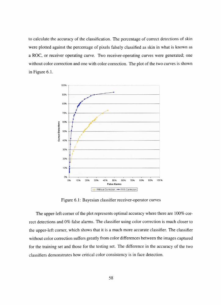
to calculate the accuracy of the classification. The percentage of correct detections of skin
were plotted against the percentage of pixels falsely classified as skin in what is known as
a ROC, or receiver operating curve. Two receiver-operating curves were generated; one
without color correction and one with color correction. The plot of the two curves is shown
in Figure 6. 1 .
t
O 40%
0% 10% 20% 30% 40% 50% 60% 70% B0% 90% 100%
False Alarms
- Without Correction Wrtft Correction
Figure 6.1: Bayesian classifier receiver-operator curves
The upper-left corner of the plot represents optimal accuracy where there are 100% cor
rect detections and 0% false alarms. The classifier using color correction is much closer to
the upper-left comer, which shows that it is a much more accurate classifier. The classifier
without color correction suffers greatly from color differences between the images captured
for the training set and those for the testing set. The difference in the accuracy of the two
classifiers demonstrates how critical color consistency is in face detection.
58
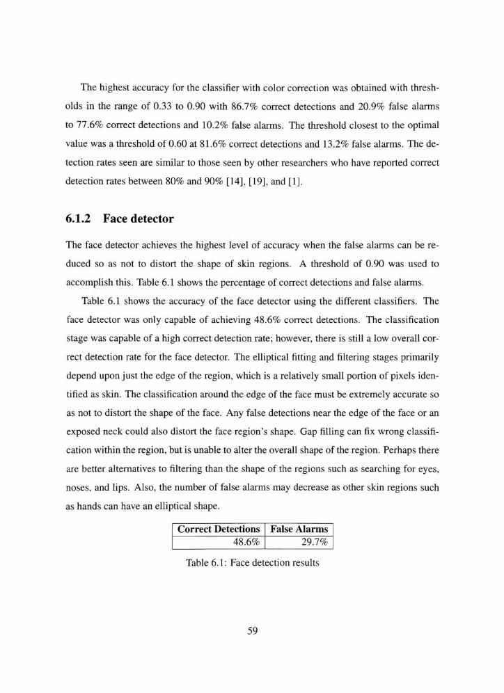
The highest accuracy for the classifier with color correction was obtained with thresh
olds in the range of 0.33 to 0.90 with 86.7% correct detections and 20.9% false alarms
to 77.6% correct detections and 10.2% false alarms. The threshold closest to the optimal
value was a threshold of 0.60 at 81.6% correct detections and 13.2% false alarms. The de
tection rates seen are similar to those seen by other researchers who have reported correct
detection rates between 80% and 90% [14], [19], and [1].
6.1.2 Face detector
The face detector achieves the highest level of accuracy when the false alarms can be re
duced so as not to distort the shape of skin regions. A threshold of 0.90 was used to
accomplish this. Table 6.1 shows the percentage of correct detections and false alarms.
Table 6.1 shows the accuracy of the face detector using the different classifiers. The
face detector was only capable of achieving 48.6% correct detections. The classification
stage was capable of a high correct detection rate; however, there is still a low overall cor
rect detection rate for the face detector. The elliptical fitting and filtering stages primarily
depend upon just the edge of the region, which is a relatively small portion of pixels iden
tified as skin. The classification around the edge of the face must be extremely accurate so
as not to distort the shape of the face. Any false detections near the edge of the face or an
exposed neck could also distort the face region's shape. Gap filling can fix wrong classifi
cation within the region, but is unable to alter the overall shape of the region. Perhaps there
are better alternatives to filtering than the shape of the regions such as searching for eyes,
noses, and lips. Also, the number of false alarms may decrease as other skin regions such
as hands can have an elliptical shape.
Correct Detections FalseAlarms
48.6% 29.7%
Table 6.1: Face detection results
59
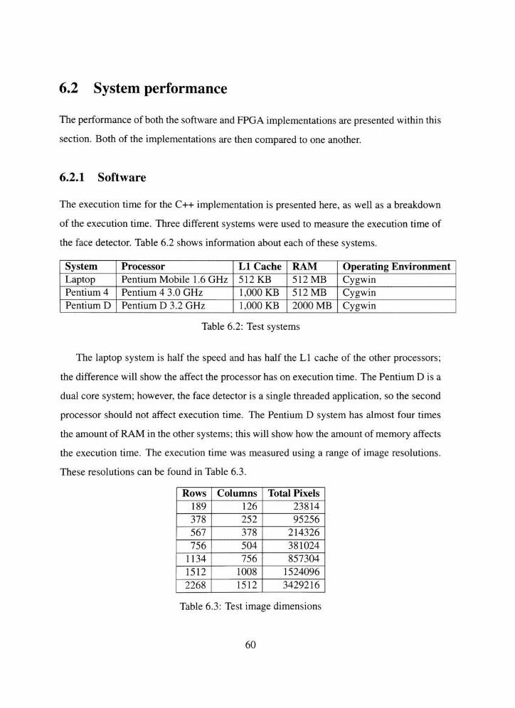
6.2 System performance
The performance of both the software and FPGA implementations are presented within this
section. Both of the implementations are then compared to one another.
6.2.1 Software
The execution time for the C++ implementation is presented here, as well as a breakdown
of the execution time. Three different systems were used to measure the execution time of
the face detector. Table 6.2 shows information about each of these systems.
System Processor LI Cache RAM Operating Environment
Laptop Pentium Mobile 1 .6 GHz 512KB 512MB Cygwin
Pentium 4 Pentium 4 3.0 GHz 1,000 KB 512MB Cygwin
Pentium D Pentium D 3.2 GHz 1,000 KB 2000MB Cygwin
Table 6.2: Test systems
The laptop system is half the speed and has half the LI cache of the other processors;
the difference will show the affect the processor has on execution time. The Pentium D is a
dual core system; however, the face detector is a single threaded application, so the second
processor should not affect execution time. The Pentium D system has almost four times
the amount ofRAM in the other systems; this will show how the amount ofmemory affects
the execution time. The execution time was measured using a range of image resolutions.
These resolutions can be found in Table 6.3.
Rows Columns Total Pixels
189 126 23814
378 252 95256
567 378 214326
756 504 381024
1134 756 857304
1512 1008 1524096
2268 1512 3429216
Table 6.3: Test image dimensions
60

Gprof, a GNU profiling tool, was used to measure the execution time and provide a
breakdown of the time spent in each component. Gcc has an optional compile flag, -pg,
used to compile in the information needed for gprof with the executable. In addition to the
-pg flag, the -03 optimization tag was used. This tag optimizes the source where possible
for maximum performance.
The execution time of a single image was too fast to gather accurate information about
the speed of the face detector, so a loop containing a set of ten images from the testing
set were used as input for the face detector. 500 detections were performed for smaller
resolution images. Less detections were done as the image size increased; 50 detections
were performed for the largest resolution.
Pentium 4M Laplop
Pentlurn 4 DesKlop
-*- Pentium D Desktop
1,000,000 2,000,000 3,000,000 4,000,000
Pixels
Figure 6.2: Face detector execution time
Figure 6.2 shows the execution times for each image resolution on each system. The
Pentium 4 and Pentium D systems produced approximately the same execution time, while
the laptop continued to be outpaced as the image resolution increased. Relatively the same
performance between the two Pentium systems showed that 512 MB of RAM was suffi
cient. The laptop system was actually faster for an image size of 126x189 pixels, but was
61
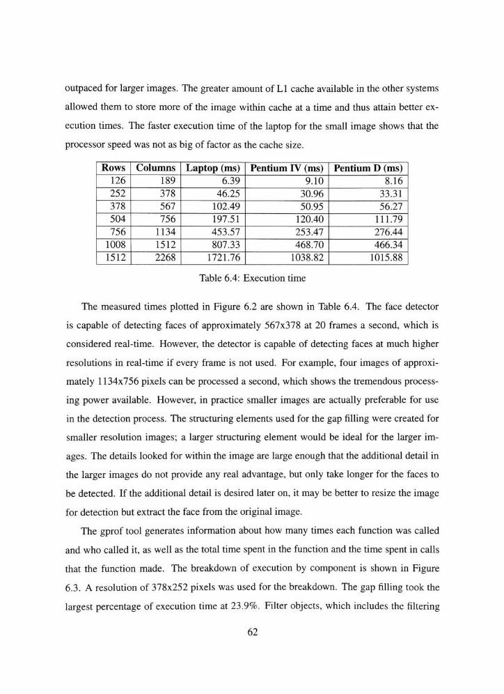
outpaced for larger images. The greater amount ofLI cache available in the other systems
allowed them to store more of the image within cache at a time and thus attain better ex
ecution times. The faster execution time of the laptop for the small image shows that the
processor speed was not as big of factor as the cache size.
Rows Columns Laptop (ms) Pentium IV (ms) Pentium D (ms)
126 189 6.39 9.10 8.16
252 378 46.25 30.96 33.31
378 567 102.49 50.95 56.27
504 756 197.51L
120.40 111.79
756 1134 453.57 253.47 276.44
1008 1512 807.33 468.70 466.34
1512 2268 1721.76 1038.82 1015.88
Table 6.4: Execution time
The measured times plotted in Figure 6.2 are shown in Table 6.4. The face detector
is capable of detecting faces of approximately 567x378 at 20 frames a second, which is
considered real-time. However, the detector is capable of detecting faces at much higher
resolutions in real-time if every frame is not used. For example, four images of approxi
mately 1134x756 pixels can be processed a second, which shows the tremendous process
ing power available. However, in practice smaller images are actually preferable for use
in the detection process. The structuring elements used for the gap filling were created for
smaller resolution images; a larger structuring element would be ideal for the larger im
ages. The details looked for within the image are large enough that the additional detail in
the larger images do not provide any real advantage, but only take longer for the faces to
be detected. If the additional detail is desired later on, it may be better to resize the image
for detection but extract the face from the original image.
The gprof tool generates information about how many times each function was called
and who called it, as well as the total time spent in the function and the time spent in calls
that the function made. The breakdown of execution by component is shown in Figure
6.3. A resolution of 378x252 pixels was used for the breakdown. The gap filling took the
largest percentage of execution time at 23.9%. Filter objects, which includes the filtering
62

Component Breakdown
Extract Faces, 3.3%Filter Objects,21.0%
Detect Objects
13.0%
FillGaps.23.9%
YCrCb Conversion,21.0%
Color Correction,17.3%
Bayesian
Classification,0.7%
Figure 6.3: Software execution time breakdown by component
stages and the elliptical fitting, were the second largest component along with YCrCb con
version at 21.0%. The Bayesian classification was the smallest at 0.7%. The component
breakdown shows that the image processing steps of YCrCb conversion, color correction,
and gap filling were the most intensive portions of processing with a combined 62.2% of
the execution time. These steps are important to improve the accuracy of the entire system,
but they also require over half of the execution time. The breakdown of the face detector's
execution time can also be looked at by function.
The functional breakdown is shown in Figure 6.4. YCrCb conversion, erosion, color
correction, dilation, connected components, and image subtraction take up 91.6% of the
execution time. The YCrCb conversion consumes the most execution time by function
at 21.0%. Erosion follows closely behind at 19.8% and then color correction at 17.3%.
The erosion and dilation algorithms are very similar in structure and combined represent
the largest portion of execution time at 34.3%. The significant time spent in the image
processing components also appears in the functional breakdown as YCrCb conversion,
color correction, erosion, and dilation consume 72.6% of execution time. The component
breakdown also showed 21.0% of the time is spent in the filtering and elliptical fitting
stages. Surprisingly, the elliptical fitting does not represent a significant enough portion of
63
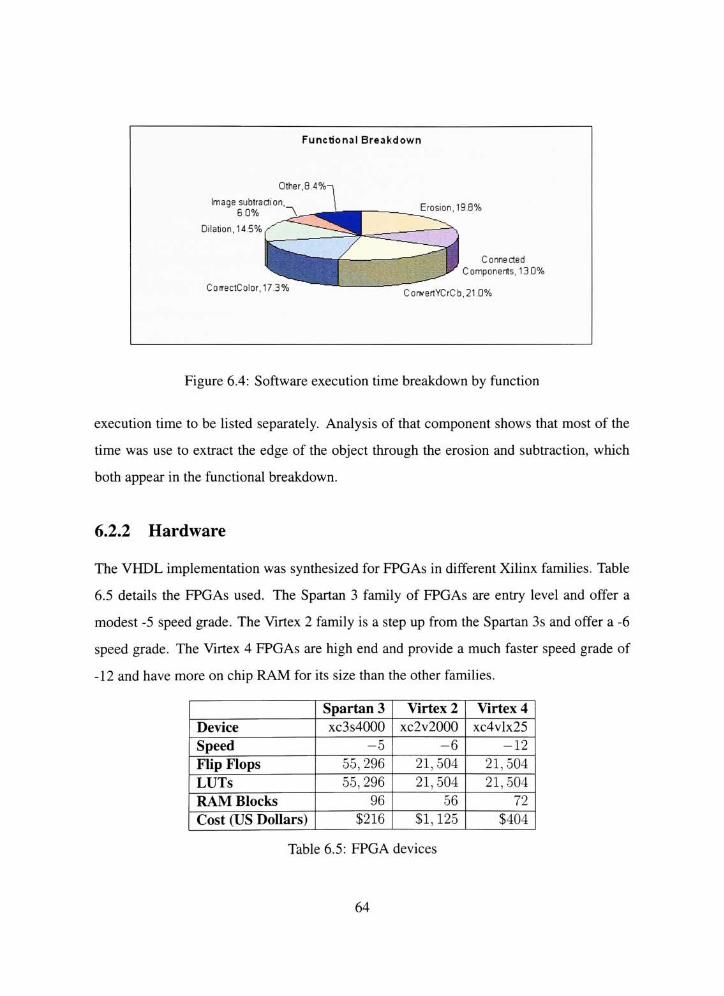
Functional Brea kd own
Other ,8 4%-.
Image subtraction,
60% ~\
Dilation, 14 5%
\ Erosion 19.8%
) Connected
Components, 13 0%
;b,210%CorrectColor,17.3%
CorwertYCrC
Figure 6.4: Software execution time breakdown by function
execution time to be listed separately. Analysis of that component shows that most of the
time was use to extract the edge of the object through the erosion and subtraction, which
both appear in the functional breakdown.
6.2.2 Hardware
The VHDL implementation was synthesized for FPGAs in different Xilinx families. Table
6.5 details the FPGAs used. The Spartan 3 family of FPGAs are entry level and offer a
modest -5 speed grade. The Virtex 2 family is a step up from the Spartan 3s and offer a -6
speed grade. The Virtex 4 FPGAs are high end and provide a much faster speed grade of
-12 and have more on chip RAM for its size than the other families.
Spartan 3 Virtex 2 Virtex 4
Device xc3s4000 xc2v2000 xc4vlx25
Speed -5 -6 -12
Flip Flops 55, 296 21,504 21,504
LUTs 55, 296 21,504 21,504
RAM Blocks 96 56 72
Cost (US Dollars) $216 $1, 125 $404
Table 6.5: FPGA devices
64

Dilation, erosion, and connected components FPGA implementations were synthesized
for each FPGA. The speed and utilization for each is shown in Table 6.6. The synthesis
for the dilation and erosion architectures produced the same results. The slowest clock
rate was on the Spartan 3, which was capable of 100MHz clock speed with less than 10%
utilization of the available flip flops and LUTs and 16% of the block RAM. The Virtex 4
provided the fastest clock rate at 178.6 MHz with 10% and 25% flip flop and LUT utiliza
tion respectively. 22% of the block RAM was used. The dilation and erosion architectures
leave a lot of room on the chip for additional logic. The connected components architecture
was not capable of the clock rate attained by the other architectures. The Spartan 3 attained
a 51.8 MHz clock rate with little flip flops and LUTs used and 50% of the RAM blocks
utilized. The Virtex 4 produced the quickest clock rate at 113.6 MHz while utilizing 1%
of the flip flops, 6% of the LUTs, and 66% of the block RAM. The connected components
architecture utilizes a large portion of the available block RAM. Connected components
on the Virtex 2 used almost all the block RAM at 85%. The large amount of block RAM
that needed to be routed from all over the chip to the actual logic is probably the reason for
lower clock speeds than the dilation and erosion architectures. In order to utilize the rest
of the FPGA with connected components, the image data would have to be stored off-chip
and streamed in. The dilation and erosion architectures are capable of utilizing much less
memory because each pixel can be stored as a bit; however, the connected components
algorithm needs 9 bits per pixel.
The dilation and erosion architectures use 34 clock cycles per block to read, 1 cycle to
process, and 32 cycles to write the result. The writes occur while the next reads happen,
so the total number of cycles would be 35 NUMBLOCKS + 32 where the additional
32 cycles is the last write when there is no read. In an image of size 256x384 pixels there
are 96 blocks, which would take 3392 cycles for a total execution time between 0.019
and 0.034 ms. The connected components architecture is not able to take advantage of
the parallelism seen in the dilation and erosion architectures and takes much longer. It is
difficult to calculate the number of cycles needed for the connected components algorithm
65
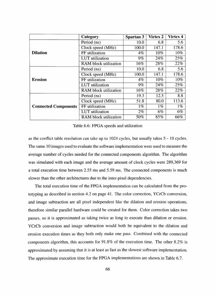
Category Spartan 3 Virtex 2 Virtex 4
Dilation
Period (ns) 10.0 6.8 5.6
Clock speed (MHz) 100.0 147.1 178.6
FF utilization 4% 10% 10%
LUT utilization 9% 24% 25%
RAM block utilization 16% 28% 22%
Erosion
Period (ns) 10.0 6.8 5.6
Clock speed (MHz) 100.0 147.1 178.6
FF utilization 4% 10% 10%
LUT utilization 9% 24% 25%
RAM block utilization 16% 28% 22%
Connected Components
Period (ns) 19.3 12.5 8.8
Clock speed (MHz) 51.8 80.0 113.6
FF utilization 1% 1% 1%
LUT utilization 2% 6% 6%
RAM block utilization 50% 85% 66%
Table 6.6: FPGA speeds and utilization
as the conflict table resolution can take up to 1024 cycles, but usually takes 5-10 cycles.
The same 10 images used to evaluate the software implementationwere used to measure the
average number of cycles needed for the connected components algorithm. The algorithm
was simulated with each image and the average amount of clock cycles were 289,369 for
a total execution time between 2.55 ms and 5.59 ms. The connected components is much
slower than the other architectures due to the inter-pixel dependencies.
The total execution time of the FPGA implementation can be calculated from the pro
totyping as described in section 4.2 on page 41. The color correction, YCrCb conversion,
and image subtraction are all pixel independent like the dilation and erosion operations,
therefore similar parallel hardware could be created for them. Color correction takes two
passes, so it is approximated as taking twice as long to execute than dilation or erosion.
YCrCb conversion and image subtraction would both be equivalent to the dilation and
erosion execution times as they both only make one pass. Combined with the connected
components algorithm, this accounts for 91.8% of the execution time. The other 8.2% is
approximated by assuming that it is at least as fast as the slowest software implementation.
The approximate execution time for the FPGA implementations are shown in Table 6.7.
66
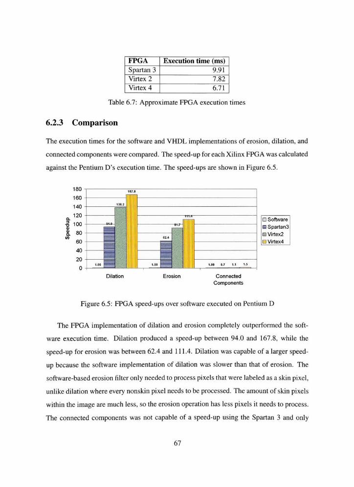
FPGA Execution time (ms)
Spartan 3 9.91
Virtex 2 7.82
Virtex 4 6.71
Table 6.7: Approximate FPGA execution times
6.2.3 Comparison
The execution times for the software and VHDL implementations of erosion, dilation, and
connected components were compared. The speed-up for eachXilinx FPGAwas calculated
against the PentiumD's execution time. The speed-ups are shown in Figure 6.5.
Dilation Erosion Connected
Components
? Software
SSpartan3
^Virtex2
D Virtex4
Figure 6.5: FPGA speed-ups over software executed on Pentium D
The FPGA implementation of dilation and erosion completely outperformed the soft
ware execution time. Dilation produced a speed-up between 94.0 and 167.8, while the
speed-up for erosion was between 62.4 and 111.4. Dilation was capable of a larger speed
up because the softwareimplementation of dilation was slower than that of erosion. The
software-based erosion filter only needed to process pixels that were labeled as a skin pixel,
unlike dilation where every nonskin pixel needs to be processed. The amount of skin pixels
within the image are much less, so the erosion operation has less pixels it needs to process.
The connected components was not capable of a speed-up using the Spartan 3 and only
67
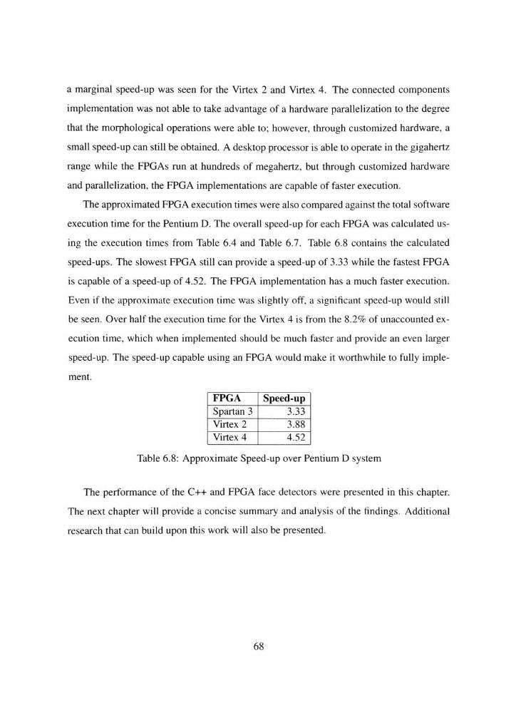
a marginal speed-up was seen for the Virtex 2 and Virtex 4. The connected components
implementation was not able to take advantage of a hardware parallelization to the degree
that the morphological operations were able to; however, through customized hardware, a
small speed-up can still be obtained. A desktop processor is able to operate in the gigahertz
range while the FPGAs run at hundreds of megahertz, but through customized hardware
and parallelization, the FPGA implementations are capable of faster execution.
The approximated FPGA execution times were also compared against the total software
execution time for the Pentium D. The overall speed-up for each FPGA was calculated us
ing the execution times from Table 6.4 and Table 6.7. Table 6.8 contains the calculated
speed-ups. The slowest FPGA still can provide a speed-up of 3.33 while the fastest FPGA
is capable of a speed-up of 4.52. The FPGA implementation has a much faster execution.
Even if the approximate execution time was slightly off, a significant speed-up would still
be seen. Over half the execution time for the Virtex 4 is from the 8.2% of unaccounted ex
ecution time, which when implemented should be much faster and provide an even larger
speed-up. The speed-up capable using an FPGA would make it worthwhile to fully imple
ment.
FPGA Speed-upSpartan 3 3.33
Virtex 2 3.88
Virtex 4 4.52
Table 6.8: Approximate Speed-up over Pentium D system
The performance of the C++ and FPGA face detectors were presented in this chapter.
The next chapter will provide a concise summary and analysis of the findings. Additional
research that can build upon this work will also be presented.
68
Chapter 7
Conclusion
The results obtained in this thesis are analyzed within this chapter. Additional research in
this area is also suggested.
7.1 Accuracy
The face detector was capable of a marginal correct detection rate of 48.6%. The correct
detection rate achieved by the Bayesian classifier was similar to those seen in other work in
spite of the low overall detection rate. The filtering portion of the detection method uses the
shape of the skin region to separate faces from other skin regions, which makes it critical
that the outline of the face region is correctly classified. While the classification is good, it
is not perfect. Gap filling is used to correct classification mistakes within the skin region;
however, this does not affect the shape of the region. Exposed skin regions attached to the
hand such as the neck will also alter the shape of the region. Besides distortions due to
miss-classifying skin pixels as nonskin, false alarms can distort the skin region's shape if
they are near the outline of the face region. The false alarm rate of 29.7% was also higher
than is desired. Other skin regions, such as hands, may have an elliptical-like shape and
not be filtered out. The findings show that filtering on the shape of the face region alone is
not a reliable method. The classifier was able to classify most of the actual skin pixels as
skin; using a method that does not rely on the outline such as the presence of eyes, noses,
or lips may be a better alternative.
69
7.2 Performance
The software-based face detector was capable of detecting faces within images of approxi
mately 378x567 pixels at real-time speed, 20 frames per second. Larger images could also
be processed in real-time if not all frames are processed, however, in practice smaller im
ages are actually preferable for use in the detection process as the extra detail is not needed.
The execution times measured for the software-based approach was mostly affected by the
size of LI cache. The Pentium 4 and Pentium D systems had twice as much LI cache and
ran almost twice as fast as the Pentium 4M system.
Analysis of the software-based face detector showed that 62.1% of the execution time
was spent in the intial image processing stages with 23.7% used for dilation and erosion.
Dilation and erosion operations were used to determine the approximate speed-up for the
image processing functionality. Connected components was also implemented to represent
functionality that was dependent on the output of previous pixels. The image processing
and connected components functionality were approximately 91.6% of the total execution
time.
A speed-up of 94.0 and 167.8 was seen for dilation and 62.4 and 111.4 for erosion
using the Virtex 4 FPGA. The erosion and dilation FPGA implementations were able to
take advantage of hardware parallelization, which significantly reduced the execution time
for those operations over the software implementations. The FPGA implementation of
the connected components algorithm was not able to attain a significant speed-up. On the
Spartan 3, the execution time was actually slower than software. The customized hardware
was capable of nearly the same execution time as the software version; however, without
considerable parallelization, the FPGA implementation did not provide a significant speed
up.
Overall a speed-up between 3.33 and 4.52 was achieved within the FPGA over the
fastest system, the Pentium D. All of the face detection components with non-trivial exe
cution time would be significantly faster in an FPGA except for the connected components
algorithm. Within software 78.6% of the time was spent processing these components. In
70
hardware, these components only represent 3.1% of the execution time. The 8.2% of soft
ware execution time that represented the remaining functions was cautiously approximated
to the execution time on the slower processor, which was 3.95 ms. This is over half the total
approximated time within hardware for the Virtex 4. In practice the FPGA implementation
should be much faster, and a greater speed-up would be realized. Connected components
was identified as the potential bottleneck in an FPGA implementation. Improvement in this
area would greatly speed-up the hardware face detection.
The FPGA version is capable of detecting faces much faster than the software version;
however, there are trade-offs for the increased performance. The software approach is bet
ter for prototyping and fine-tuning the system when design can change extensively. In
addition, the software version does not require any special hardware, an FPGA implemen
tation would be best used to improve the execution time of an existing software-based face
detection method and not development of a new approach.
7.3 Future Research
7.3.1 Change filtering method
Filtering using the shape of the face did not produce a high correct detection rate. The
method depends on too small a portion of the skin regions to have the desired accuracy.
Also, other skin regions such as hands may have an elliptical region and would be falsely
classified as faces. Perhaps amethod that searches for the presence of facial features within
the skin regions would be a better filtering method.
7.3.2 Improve parallelism in connected components algorithm
The FPGA implementation of the connected components algorithm did not obtain the
speed-up seen with the dilation anderosion implementations. The high-level of parallelism
within the dilation and erosion filters made the large speed-up possible. The connected
71

components algorithm depends upon the results ofpixels processed before the current pixel,
which makes the algorithm more difficult to parallize; however, a set of rows could be read
into an array of connected components processing elements. The result of one processing
element can then be passed to the subsequent elements that depend on it's result in order
to add additional parallelism to the system. Also, storing the conflict table in a register
would allow for multiple pixels to attain their conflict resolved value in the second pass
simultaneously and provide additional parallelism in the hardware.
7.3.3 Fully implemented FPGA-based face detector
The face detector was only partially implemented to approximate the potential perfor
mance. The hardware is capable ofmuch faster detection speeds than the software version.
Implementing the entire detector within an FPGA would take advantage of the increased
speed. The approximated execution time was a baseline of possible performance and cau
tiously approximated the other functionality. In practice, this face detector would probably
be even faster than a software implementation.
72

Bibliography
[1] Jason Brand and John S. Mason. A comparative assessment of three approaches
to pixel-level human skin-detection. In IEEE International Conference on Pattern
Recognition, pages 5056-5059, Barcelona, Spain, September 2000.
[2] O. Deforges and N. Normand. A generic systolic processor for real time grayscale
morphology. In IEEE International Conference on Acoustics, Speech, and Signal
Processing, pages 3331-3334, Istanbul, Turkey, June 2000.
[3] Andrew Fitzgibbon, Maurizio Pilu, and Robert B. Fisher. Direct least square fitting
of ellipses. IEEE Trans. Pattern Analysis andMachine Intelligence, 21(5):476-480,
May 1999.
[4] David A. Forsyth and Jean Ponce. Computer Vision: A Modern Approach. Prentice
Hall, Upper Saddle River, New Jersey, 2002.
[5] Rafael C. Gonzalez and Richard E. Woods. Digital Image Processing. Prentice Hall,
Upper Saddle River, New Jersey, 2001.
[6] R.-L. Hsu, M. Adbel-Mottaleb, and A.K. Jain. Face detection in color images. IEEE
Trans. Pattern Analysis andMachine Intelligence, 24(0):696-707, May 2002.
[7] A. C. Loui, C. N. Judice, and S. Liu. An image database for benchmarking of auto
matic face detection and recognition algorithms. In Proc. IEEE Conference on Image
Processing, pages 146-150, Chicago, Illinois, USA, October 1998.
[8] A. M. Martinez and R. Benavente. The AR face database. CVC Technical Report, 24,
June 1998.
[9] Soohwan Ong andMyung H. Sunwoo. A new cost-effectivemorphological filter chip.
In IEEEWorkshop on Signal Processing Systems, pages 421-430, Boston, MA, USA,
November 1997.
73

[10] P. J. Phillips, H. Moon, S. A. Rizvi, and P. J. Rauss. The FERET evaluation method
ology for face recognition algorithms. IEEE Trans. Pattern Analysis and Machine
Intelligence, 22:1090-1104, October 2000.
[11] Ashley Rasquinha and N. Ranganathan. C3L: A chip for connected components. In
10th International Conference on VLSI Design, pages 446-450, Hyderabad, India,
January 1997.
[12] Maricor Soriano, BirgittaMartinkauppi, Sami Huovinen, andMika Laaksonen. Skin
detection in video under changing illumination conditions. In International Confer
ence on Pattern Recognition, pages 1839-1842, Barcelona, Spain, September 2000.
[13] Sanun Srisuk andWerasak Kurutach. A new robust face detection in color images. In
IEEE International Conference on Automatic Face and Gesture Recognition, pages
306-311, Washington, DC, USA, May 2002.
[14] Vladimir Vezhnevets, Vassili Sazonov, and Alia Andreeva. A survey on pixel-based
skin color detection techniques. In Proc. Graphicon-2003,pages 85-92, September
2003.
[15] Haiyuan Wu, Qian Chen, and Masahiko Yachida. Face detection from color images
using a fuzzy pattern matching method. IEEE Trans. Pattern Analysis andMachine
Intelligence, 21(6):557-563, June 1999.
[16] Ming-Hsuan Yang. Recent advances in face detection. In IEEE Conference on Pattern
Recognition, Cambridge, UK, August 2004.
[17] Ming-Hsuan Yang, David J. Kriegman, and Narendra Ahuja. Detecting faces in im
ages: A survey. IEEE Trans. PatternAnalysis andMachine Intelligence, 24(l):34-58,
January 2002.
[18] S. W Yang, M. H. Sheu, H. E. Chien H. H. Wu, P. K. Weng, and Y. Y. Wu. VLSI
architecture design for a fast parallel label assignment in binary image. In IEEE
International Symposium on Circuits and Systems, pages 2393-2396, Kobe, Japan,
May 2005.
[19] Benjamin D. Zarit, Boaz J. Super, and Francis K. H. Quek. Comparison of five color
models in skin pixel classification. In RATFG-RTS '99: Proceedings of the Inter
national Workshop on Recognition, Analysis, and Tracking ofFaces and Gestures in
Real-Time Systems, Corfu, Greece, September 1999. IEEE Computer Society.
74