FPNN: Field Probing Neural Networks for 3D Data

Yangyan Li1,2 Sören Pirk1 Hao Su1 Charles R. Qi1 Leonidas J. Guibas11Stanford University, USA 2Shandong University, China

AbstractBuilding discriminative representations for 3D data has been an important task incomputer graphics and computer vision research. Convolutional Neural Networks(CNNs) have shown to operate on 2D images with great success for a varietyof tasks. Lifting convolution operators to 3D (3DCNNs) seems like a plausibleand promising next step. Unfortunately, the computational complexity of 3DCNNs grows cubically with respect to voxel resolution. Moreover, since most 3Dgeometry representations are boundary based, occupied regions do not increaseproportionately with the size of the discretization, resulting in wasted computation.In this work, we represent 3D spaces as volumetric fields, and propose a noveldesign that employs field probing filters to efficiently extract features from them.Each field probing filter is a set of probing points — sensors that perceive thespace. Our learning algorithm optimizes not only the weights associated with theprobing points, but also their locations, which deforms the shape of the probingfilters and adaptively distributes them in 3D space. The optimized probing pointssense the 3D space “intelligently”, rather than operating blindly over the entiredomain. We show that field probing is significantly more efficient than 3DCNNs,while providing state-of-the-art performance, on classification tasks for 3D objectrecognition benchmark datasets.

1 Introduction

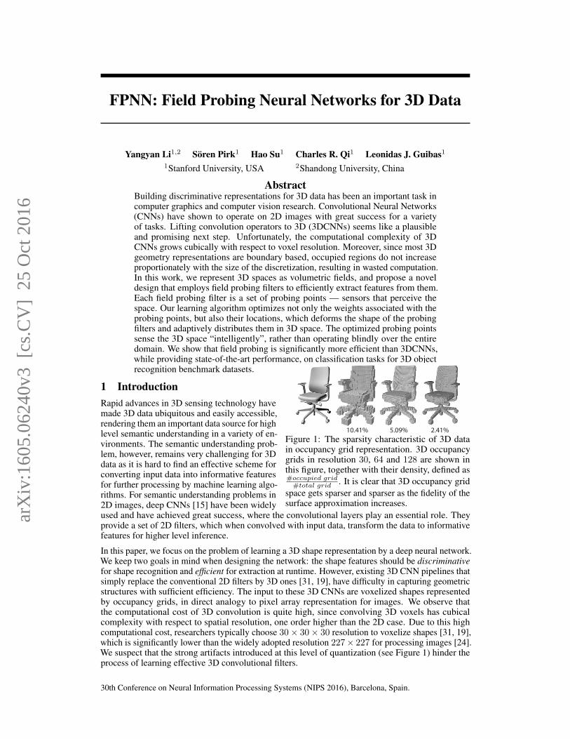
10.41% 5.09% 2.41%Figure 1: The sparsity characteristic of 3D datain occupancy grid representation. 3D occupancygrids in resolution 30, 64 and 128 are shown inthis figure, together with their density, defined as#occupied grid#total grid . It is clear that 3D occupancy grid

space gets sparser and sparser as the fidelity of thesurface approximation increases.

Rapid advances in 3D sensing technology havemade 3D data ubiquitous and easily accessible,rendering them an important data source for highlevel semantic understanding in a variety of en-vironments. The semantic understanding prob-lem, however, remains very challenging for 3Ddata as it is hard to find an effective scheme forconverting input data into informative featuresfor further processing by machine learning algo-rithms. For semantic understanding problems in2D images, deep CNNs [15] have been widelyused and have achieved great success, where the convolutional layers play an essential role. Theyprovide a set of 2D filters, which when convolved with input data, transform the data to informativefeatures for higher level inference.

In this paper, we focus on the problem of learning a 3D shape representation by a deep neural network.We keep two goals in mind when designing the network: the shape features should be discriminativefor shape recognition and efficient for extraction at runtime. However, existing 3D CNN pipelines thatsimply replace the conventional 2D filters by 3D ones [31, 19], have difficulty in capturing geometricstructures with sufficient efficiency. The input to these 3D CNNs are voxelized shapes representedby occupancy grids, in direct analogy to pixel array representation for images. We observe thatthe computational cost of 3D convolution is quite high, since convolving 3D voxels has cubicalcomplexity with respect to spatial resolution, one order higher than the 2D case. Due to this highcomputational cost, researchers typically choose 30× 30× 30 resolution to voxelize shapes [31, 19],which is significantly lower than the widely adopted resolution 227× 227 for processing images [24].We suspect that the strong artifacts introduced at this level of quantization (see Figure 1) hinder theprocess of learning effective 3D convolutional filters.

30th Conference on Neural Information Processing Systems (NIPS 2016), Barcelona, Spain.

arX

iv:1

605.

0624

0v3

[cs

.CV

] 2

5 O

ct 2

016

(a) (b) (c) (d)

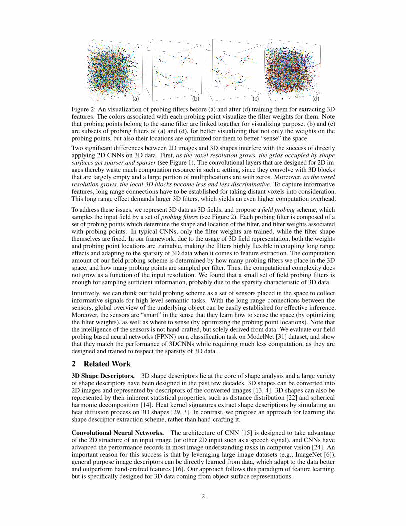
Figure 2: An visualization of probing filters before (a) and after (d) training them for extracting 3Dfeatures. The colors associated with each probing point visualize the filter weights for them. Notethat probing points belong to the same filter are linked together for visualizing purpose. (b) and (c)are subsets of probing filters of (a) and (d), for better visualizing that not only the weights on theprobing points, but also their locations are optimized for them to better “sense” the space.Two significant differences between 2D images and 3D shapes interfere with the success of directlyapplying 2D CNNs on 3D data. First, as the voxel resolution grows, the grids occupied by shapesurfaces get sparser and sparser (see Figure 1). The convolutional layers that are designed for 2D im-ages thereby waste much computation resource in such a setting, since they convolve with 3D blocksthat are largely empty and a large portion of multiplications are with zeros. Moreover, as the voxelresolution grows, the local 3D blocks become less and less discriminative. To capture informativefeatures, long range connections have to be established for taking distant voxels into consideration.This long range effect demands larger 3D filters, which yields an even higher computation overhead.

To address these issues, we represent 3D data as 3D fields, and propose a field probing scheme, whichsamples the input field by a set of probing filters (see Figure 2). Each probing filter is composed of aset of probing points which determine the shape and location of the filter, and filter weights associatedwith probing points. In typical CNNs, only the filter weights are trained, while the filter shapethemselves are fixed. In our framework, due to the usage of 3D field representation, both the weightsand probing point locations are trainable, making the filters highly flexible in coupling long rangeeffects and adapting to the sparsity of 3D data when it comes to feature extraction. The computationamount of our field probing scheme is determined by how many probing filters we place in the 3Dspace, and how many probing points are sampled per filter. Thus, the computational complexity doesnot grow as a function of the input resolution. We found that a small set of field probing filters isenough for sampling sufficient information, probably due to the sparsity characteristic of 3D data.

Intuitively, we can think our field probing scheme as a set of sensors placed in the space to collectinformative signals for high level semantic tasks. With the long range connections between thesensors, global overview of the underlying object can be easily established for effective inference.Moreover, the sensors are “smart” in the sense that they learn how to sense the space (by optimizingthe filter weights), as well as where to sense (by optimizing the probing point locations). Note thatthe intelligence of the sensors is not hand-crafted, but solely derived from data. We evaluate our fieldprobing based neural networks (FPNN) on a classification task on ModelNet [31] dataset, and showthat they match the performance of 3DCNNs while requiring much less computation, as they aredesigned and trained to respect the sparsity of 3D data.

2 Related Work3D Shape Descriptors. 3D shape descriptors lie at the core of shape analysis and a large varietyof shape descriptors have been designed in the past few decades. 3D shapes can be converted into2D images and represented by descriptors of the converted images [13, 4]. 3D shapes can also berepresented by their inherent statistical properties, such as distance distribution [22] and sphericalharmonic decomposition [14]. Heat kernel signatures extract shape descriptions by simulating anheat diffusion process on 3D shapes [29, 3]. In contrast, we propose an approach for learning theshape descriptor extraction scheme, rather than hand-crafting it.

Convolutional Neural Networks. The architecture of CNN [15] is designed to take advantageof the 2D structure of an input image (or other 2D input such as a speech signal), and CNNs haveadvanced the performance records in most image understanding tasks in computer vision [24]. Animportant reason for this success is that by leveraging large image datasets (e.g., ImageNet [6]),general purpose image descriptors can be directly learned from data, which adapt to the data betterand outperform hand-crafted features [16]. Our approach follows this paradigm of feature learning,but is specifically designed for 3D data coming from object surface representations.

2

CNNs on Depth and 3D Data. With rapid advances in 3D sensing technology, depth has becameavailable as an additional information channel beyond color. Such 2.5D data can be represented asmultiple channel images, and processed by 2D CNNs [26, 10, 8]. Wu et al. [31] in a pioneeringpaper proposed to extend 2D CNNs to process 3D data directly (3D ShapeNets). A similar approach(VoxNet) was proposed in [19]. However, such approaches cannot work on high resolution 3D data, asthe computational complexity is a cubic function of the voxel grid resolution. Since CNNs for imageshave been extensively studied, 3D shapes can be rendered into 2D images, and be represented bythe CNN features of the images [25, 28], which, surprisingly, outperforms any 3D CNN approaches,in a 3D shape classification task. Recently, Qi et al. [23] presented an extensive study of thesevolumetric and multi-view CNNs and refreshed the performance records. In this work, we propose afeature learning approach that is specifically designed to take advantage of the sparsity of 3D data,and compare against results reported in [23]. Note that our method was designed without explicitconsideration of deformable objects, which is a purely extrinsic construction. While 3D data isrepresented as meshes, neural networks can benefit from intrinsic constructions[17, 18, 1, 2] to learnobject invariance to isometries, thus require less training data for handling deformable objects.

Our method can be viewed as an efficient scheme of sparse coding[7]. The learned weights of eachprobing curve can be interpreted as the entries of the coding matrix in the sparse coding framework.Compared with conventional sparse coding, our framework is not only computationally more tractable,but also enables an end-to-end learning system.

3 Field Probing Neural Network

3.1 Input 3D Fields

(a)

(b)

(c)

(d)

(e)

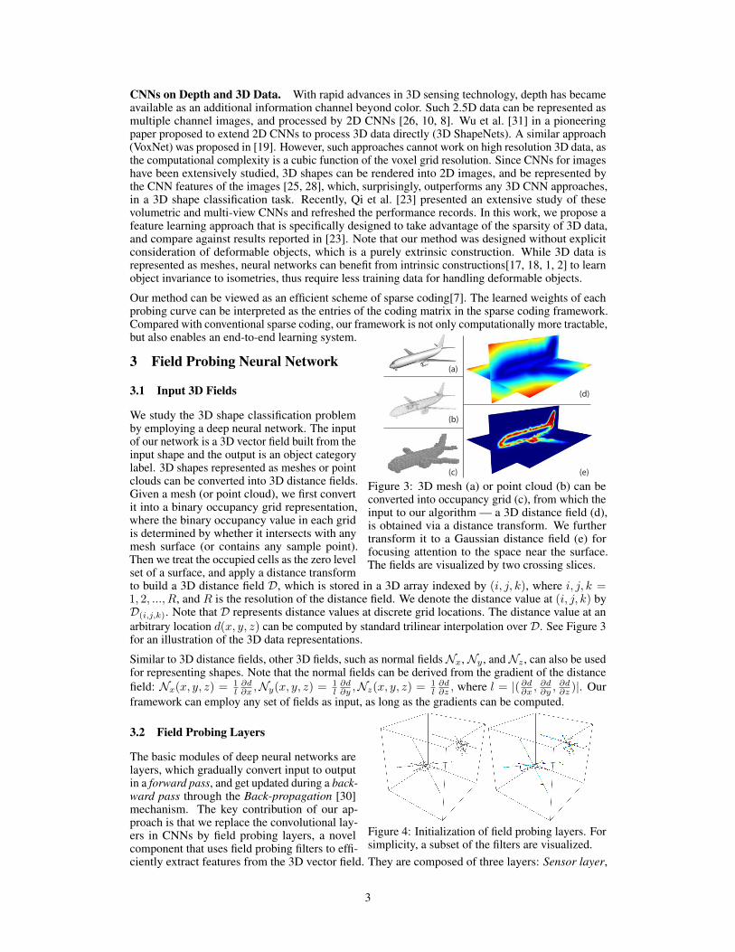
Figure 3: 3D mesh (a) or point cloud (b) can beconverted into occupancy grid (c), from which theinput to our algorithm — a 3D distance field (d),is obtained via a distance transform. We furthertransform it to a Gaussian distance field (e) forfocusing attention to the space near the surface.The fields are visualized by two crossing slices.

We study the 3D shape classification problemby employing a deep neural network. The inputof our network is a 3D vector field built from theinput shape and the output is an object categorylabel. 3D shapes represented as meshes or pointclouds can be converted into 3D distance fields.Given a mesh (or point cloud), we first convertit into a binary occupancy grid representation,where the binary occupancy value in each gridis determined by whether it intersects with anymesh surface (or contains any sample point).Then we treat the occupied cells as the zero levelset of a surface, and apply a distance transformto build a 3D distance field D, which is stored in a 3D array indexed by (i, j, k), where i, j, k =1, 2, ..., R, and R is the resolution of the distance field. We denote the distance value at (i, j, k) byD(i,j,k). Note that D represents distance values at discrete grid locations. The distance value at anarbitrary location d(x, y, z) can be computed by standard trilinear interpolation over D. See Figure 3for an illustration of the 3D data representations.

Similar to 3D distance fields, other 3D fields, such as normal fieldsNx,Ny , andNz , can also be usedfor representing shapes. Note that the normal fields can be derived from the gradient of the distancefield: Nx(x, y, z) = 1

l∂d∂x ,Ny(x, y, z) =

1l∂d∂y ,Nz(x, y, z) =

1l∂d∂z , where l = |( ∂d∂x ,

∂d∂y ,

∂d∂z )|. Our

framework can employ any set of fields as input, as long as the gradients can be computed.

3.2 Field Probing Layers

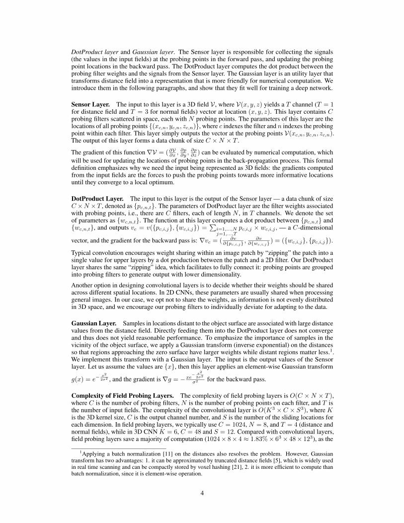
Figure 4: Initialization of field probing layers. Forsimplicity, a subset of the filters are visualized.

The basic modules of deep neural networks arelayers, which gradually convert input to outputin a forward pass, and get updated during a back-ward pass through the Back-propagation [30]mechanism. The key contribution of our ap-proach is that we replace the convolutional lay-ers in CNNs by field probing layers, a novelcomponent that uses field probing filters to effi-ciently extract features from the 3D vector field. They are composed of three layers: Sensor layer,

3

DotProduct layer and Gaussian layer. The Sensor layer is responsible for collecting the signals(the values in the input fields) at the probing points in the forward pass, and updating the probingpoint locations in the backward pass. The DotProduct layer computes the dot product between theprobing filter weights and the signals from the Sensor layer. The Gaussian layer is an utility layer thattransforms distance field into a representation that is more friendly for numerical computation. Weintroduce them in the following paragraphs, and show that they fit well for training a deep network.

Sensor Layer. The input to this layer is a 3D field V , where V(x, y, z) yields a T channel (T = 1for distance field and T = 3 for normal fields) vector at location (x, y, z). This layer contains Cprobing filters scattered in space, each with N probing points. The parameters of this layer are thelocations of all probing points {(xc,n, yc,n, zc,n)}, where c indexes the filter and n indexes the probingpoint within each filter. This layer simply outputs the vector at the probing points V(xc,n, yc,n, zc,n).The output of this layer forms a data chunk of size C ×N × T .

The gradient of this function∇V = (∂V∂x ,∂p∂y ,

∂p∂z ) can be evaluated by numerical computation, which

will be used for updating the locations of probing points in the back-propagation process. This formaldefinition emphasizes why we need the input being represented as 3D fields: the gradients computedfrom the input fields are the forces to push the probing points towards more informative locationsuntil they converge to a local optimum.

DotProduct Layer. The input to this layer is the output of the Sensor layer — a data chunk of sizeC×N ×T , denoted as {pc,n,t}. The parameters of DotProduct layer are the filter weights associatedwith probing points, i.e., there are C filters, each of length N , in T channels. We denote the setof parameters as {wc,n,t}. The function at this layer computes a dot product between {pc,n,t} and{wc,n,t}, and outputs vc = v({pc,i,j}, {wc,i,j}) =

∑i=1,...,Nj=1,...,T

pc,i,j × wc,i,j , — a C-dimensional

vector, and the gradient for the backward pass is: ∇vc = ( ∂v∂{pc,i,j} ,

∂v∂{wc,i,j} ) = ({wc,i,j}, {pc,i,j}).

Typical convolution encourages weight sharing within an image patch by “zipping” the patch into asingle value for upper layers by a dot production between the patch and a 2D filter. Our DotProductlayer shares the same “zipping” idea, which facilitates to fully connect it: probing points are groupedinto probing filters to generate output with lower dimensionality.

Another option in designing convolutional layers is to decide whether their weights should be sharedacross different spatial locations. In 2D CNNs, these parameters are usually shared when processinggeneral images. In our case, we opt not to share the weights, as information is not evenly distributedin 3D space, and we encourage our probing filters to individually deviate for adapting to the data.

Gaussian Layer. Samples in locations distant to the object surface are associated with large distancevalues from the distance field. Directly feeding them into the DotProduct layer does not convergeand thus does not yield reasonable performance. To emphasize the importance of samples in thevicinity of the object surface, we apply a Gaussian transform (inverse exponential) on the distancesso that regions approaching the zero surface have larger weights while distant regions matter less.1.We implement this transform with a Gaussian layer. The input is the output values of the Sensorlayer. Let us assume the values are {x}, then this layer applies an element-wise Gaussian transform

g(x) = e−x2

2σ2 , and the gradient is∇g = −xe− x2

2σ2

σ2 for the backward pass.

Complexity of Field Probing Layers. The complexity of field probing layers is O(C ×N × T ),where C is the number of probing filters, N is the number of probing points on each filter, and T isthe number of input fields. The complexity of the convolutional layer is O(K3 × C × S3), where Kis the 3D kernel size, C is the output channel number, and S is the number of the sliding locations foreach dimension. In field probing layers, we typically use C = 1024, N = 8, and T = 4 (distance andnormal fields), while in 3D CNN K = 6, C = 48 and S = 12. Compared with convolutional layers,field probing layers save a majority of computation (1024× 8× 4 ≈ 1.83%× 63 × 48× 123), as the

1Applying a batch normalization [11] on the distances also resolves the problem. However, Gaussiantransform has two advantages: 1. it can be approximated by truncated distance fields [5], which is widely usedin real time scanning and can be compactly stored by voxel hashing [21], 2. it is more efficient to compute thanbatch normalization, since it is element-wise operation.

4

probing filters in field probing layers are capable of learning where to “sense”, whereas convolutionallayers exhaustively examine everywhere by sliding the 3D kernels.

Initialization of Field Probing Layers. There are two sets of parameters: the probing pointlocations and the weights associated with them. To encourage the probing points to explore as manypotential locations as possible, we initialize them to be widely distributed in the input fields. Wefirst divide the space into G × G × G grids and then generate P filters in each grid. Each filteris initialized as a line segment with a random orientation, a random length in [llow, lhigh] (we use[llow, lhigh] = [0.2, 0.8] ∗ R by default), and a random center point within the grid it belongs to(Figure 4 left). Note that a probing filter spans distantly in the 3D space, so they capture long rangeeffects well. This is a property that distinguishes our design from those convolutional layers, as theyhave to increase the kernel size to capture long range effects, at the cost of increased complexity. Theweights of field probing filters are initialized by the Xavier scheme [9]. In Figure 4 right, weights fordistance field are visualized by probing point colors and weights for normal fields by arrows attachedto each probing point.

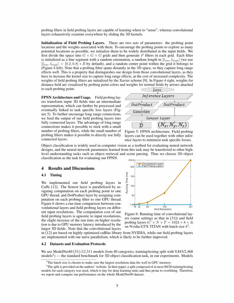
Figure 5: FPNN architecture. Field probinglayers can be used together with other infer-ence layers to minimize task specific losses.

FPNN Architecture and Usage. Field probing lay-ers transform input 3D fields into an intermediaterepresentation, which can further be processed andeventually linked to task specific loss layers (Fig-ure 5). To further encourage long range connections,we feed the output of our field probing layers intofully connected layers. The advantage of long rangeconnections makes it possible to stick with a smallnumber of probing filters, while the small number ofprobing filters makes it possible to directly use fullyconnected layers.

Object classification is widely used in computer vision as a testbed for evaluating neural networkdesigns, and the neural network parameters learned from this task may be transferred to other high-level understanding tasks such as object retrieval and scene parsing. Thus we choose 3D objectclassification as the task for evaluating our FPNN.

4 Results and Discussions4.1 Timing

Grid Resolution16 32 64 128 227

Ru

nnin

g T

ime

(ms)

1.99

50

100

150

200

234.9

Convolutional LayersField Probing Layers

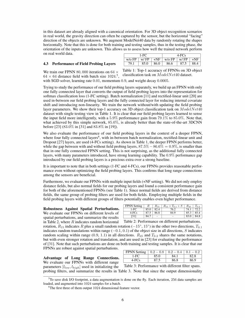
Figure 6: Running time of convolutional lay-ers (same settings as that in [31]) and fieldprobing layers (C ×N × T = 1024× 8× 4)on Nvidia GTX TITAN with batch size 83.

We implemented our field probing layers inCaffe [12]. The Sensor layer is parallelized by as-signing computation on each probing point to oneGPU thread, and DotProduct layer by assigning com-putation on each probing filter to one GPU thread.Figure 6 shows a run time comparison between con-vonlutional layers and field probing layers on differ-ent input resolutions. The computation cost of ourfield probing layers is agnostic to input resolutions,the slight increase of the run time on higher resolu-tion is due to GPU memory latency introduced by thelarger 3D fields. Note that the convolutional layersin [12] are based on highly optimized cuBlas library from NVIDIA, while our field probing layersare implemented with our naive parallelism, which is likely to be further improved.

4.2 Datasets and Evaluation Protocols

We use ModelNet40 [31] (12,311 models from 40 categories, training/testing split with 9,843/2,468models4) — the standard benchmark for 3D object classification task, in our experiments. Models

3The batch size is chosen to make sure the largest resolution data fits well in GPU memory.4The split is provided on the authors’ website. In their paper, a split composed of at most 80/20 training/testing

models for each category was used, which is tiny for deep learning tasks and thus prone to overfitting. Therefore,we report and compare our performance on the whole ModelNet40 dataset.

5

in this dataset are already aligned with a canonical orientation. For 3D object recognition scenariosin real world, the gravity direction can often be captured by the sensor, but the horizontal “facing”direction of the objects are unknown. We augment ModelNet40 data by randomly rotating the shapeshorizontally. Note that this is done for both training and testing samples, thus in the testing phase, theorientation of the inputs are unknown. This allows us to assess how well the trained network performon real world data.

4.3 Performance of Field Probing Layers

1-FC 4-FCsw/o FP w/ FP +NF w/o FP w/ FP +NF

79.1 85.0 86.0 86.6 87.5 88.4

Table 1: Top-1 accuracy of FPNNs on 3D objectclassification task on ModelNet40 dataset.

We train our FPNN 80, 000 iterations on 64 ×64 × 64 distance field with batch size 1024.5,with SGD solver, learning rate 0.01, momentum 0.9, and weight decay 0.0005.

Trying to study the performance of our field probing layers separately, we build up an FPNN with onlyone fully connected layer that converts the output of field probing layers into the representation forsoftmax classification loss (1-FC setting). Batch normalization [11] and rectified-linear unit [20] areused in-between our field probing layers and the fully connected layer for reducing internal covariateshift and introducing non-linearity. We train the network without/with updating the field probinglayer parameters. We show their top-1 accuracy on 3D object classification task on ModelNet40dataset with single testing view in Table 1. It is clear that our field probing layers learned to sensethe input field more intelligently, with a 5.9% performance gain from 79.1% to 85.0%. Note that,what achieved by this simple network, 85.0%, is already better than the state-of-the-art 3DCNNbefore [23] (83.0% in [31] and 83.8% in [19]).

We also evaluate the performance of our field probing layers in the context of a deeper FPNN,where four fully connected layers6, with in-between batch normalization, rectified-linear unit andDropout [27] layers, are used (4-FCs setting). As shown in Table 1, the deeper FPNN performs better,while the gap between with and without field probing layers, 87.5%−86.6% = 0.9%, is smaller thanthat in one fully connected FPNN setting. This is not surprising, as the additional fully connectedlayers, with many parameters introduced, have strong learning capability. The 0.9% performance gapintroduced by our field probing layers is a precious extra over a strong baseline.

It is important to note that in both settings (1-FC and 4-FCs), our FPNNs provides reasonable perfor-mance even without optimizing the field probing layers. This confirms that long range connectionsamong the sensors are beneficial.

Furthermore, we evaluate our FPNNs with multiple input fields (+NF setting). We did not only employdistance fields, but also normal fields for our probing layers and found a consistent performance gainfor both of the aforementioned FPNNs (see Table 1). Since normal fields are derived from distancefields, the same group of probing filters are used for both fields. Employing multiple fields in thefield probing layers with different groups of filters potentially enables even higher performance.

FPNN Setting R R15 R15 + T0.1 + S R45 T0.21-FC 85.0 82.4 76.2 74.1 72.24-FCs 87.5 86.8 84.9 85.3 85.4[31] 84.7 - - 83.0 84.8

Table 2: Performance on different perturbations.

Robustness Against Spatial Perturbations.We evaluate our FPNNs on different levels ofspatial perturbations, and summarize the resultsin Table 2, where R indicates random horizontalrotation, R15 indicates R plus a small random rotation (−15◦, 15◦) in the other two directions, T0.1indicates random translations within range (−0.1, 0.1) of the object size in all directions, S indicatesrandom scaling within range (0.9, 1.1) in all directions. R45 and T0.2 shares the same notations,but with even stronger rotation and translation, and are used in [23] for evaluating the performanceof [31]. Note that such perturbations are done on both training and testing samples. It is clear that ourFPNNs are robust against spatial perturbations.

FPNN Setting 0.2− 0.8 0.2− 0.4 0.1− 0.21-FC 85.0 84.1 82.84-FCs 87.5 86.8 86.9

Table 3: Performance with different filter spans.

Advantage of Long Range Connections.We evaluate our FPNNs with different rangeparameters [llow, lhigh] used in initializing theprobing filters, and summarize the results in Table 3. Note that since the output dimensionality

5To save disk I/O footprint, a data augmentation is done on the fly. Each iteration, 256 data samples areloaded, and augmented into 1024 samples for a batch.

6The first three of them output 1024 dimensional feature vector.

6

of our field probing layers is low enough to be directly feed into fully connected layers, distantsensor information is directly coupled by them. This is a desirable property, however, it poses thedifficulty to study the advantage of field probing layers in coupling long range information separately.Table 3 shows that even if the following fully connected layer has the capability to couple distanceinformation, the long range connections introduced in our field probing layers are beneficial.

FPNN Setting 16× 16× 16 32× 32× 32 64× 64× 64

1-FC 84.2 84.5 85.04-FCs 87.3 87.3 87.5

Table 4: Performance on different field resolutions.

Performance on Different Field Resolutions.We evaluate our FPNNs on different input fieldresolutions, and summarize the results in Table 4.Higher resolution input fields can represent in-put data more accurately, and Table 4 shows that our FPNN can take advantage of the more accuraterepresentations. Since the computation cost of our field probing layers is agnostic to the resolutionof the data representation, higher resolution input fields are preferred for better performance, whilecoupling with efficient data structures reduces the I/O footprint.

“Sharpness” of Gaussian Layer. The σ hyper-parameter in Gaussian layer controls how “sharp”is the transform. We select its value empirically in our experiments, and the best performance is givenwhen we use σ ≈ 10% of the object size. Smaller σ slightly hurts the performance (≈ 1%), but hasthe potential of reducing I/O footprint.

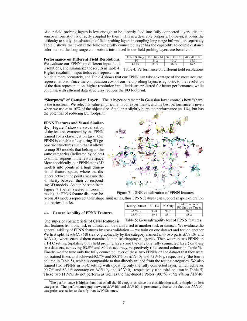
Figure 7: t-SNE visualization of FPNN features.

FPNN Features and Visual Similar-ity. Figure 7 shows a visualizationof the features extracted by the FPNNtrained for a classification task. OurFPNN is capable of capturing 3D ge-ometric structures such that it allowsto map 3D models that belong to thesame categories (indicated by colors)to similar regions in the feature space.More specifically, our FPNN maps 3Dmodels into points in a high dimen-sional feature space, where the dis-tances between the points measure thesimilarity between their correspond-ing 3D models. As can be seen fromFigure 7 (better viewed in zoominmode), the FPNN feature distances be-tween 3D models represent their shape similarities, thus FPNN features can support shape explorationand retrieval tasks.

4.4 Generalizability of FPNN Features

Testing Dataset FP+FC FC Only FP+FC on SourceFC Only on Target

MN401 93.8 90.7 92.7MN402 89.4 85.1 88.2

Table 5: Generalizability test of FPNN features.One superior characteristic of CNN features isthat features from one task or dataset can be transferred to another task or dataset. We evaluate thegeneralizability of FPNN features by cross validation — we train on one dataset and test on another.We first split ModelNet40 (lexicographically by the category names) into two parts MN401 andMN402, where each of them contains 20 non-overlapping categories. Then we train two FPNNs ina 1-FC setting (updating both field probing layers and the only one fully connected layer) on thesetwo datasets, achieving 93.8% and 89.4% accuracy, respectively (the second column in Table 5).7Finally, we fine tune only the fully connected layer of these two FPNNs on the dataset that they werenot trained from, and achieved 92.7% and 88.2% on MN401 and MN402, respectively (the fourthcolumn in Table 5), which is comparable to that directly trained from the testing categories. We alsotrained two FPNNs in 1-FC setting with updating only the fully connected layer, which achieves90.7% and 85.1% accuracy on MN401 and MN402, respectively (the third column in Table 5).These two FPNNs do not perform as well as the fine-tuned FPNNs (90.7% < 92.7% on MN401

7The performance is higher than that on all the 40 categories, since the classification task is simpler on lesscategories. The performance gap between MN401 and MN402 is presumably due to the fact that MN401categories are easier to classify than MN402 ones.

7

and 85.1% < 88.2% on MN402), although all of them only update the fully connected layer. Theseexperiments show that the field probing filters learned from one dataset can be applied to another one.

4.5 Comparison with State-of-the-artOur FPNN [23]

(4-FCs+NF) SubvolSup+BN MVCNN-MultiRes88.4 88.8 93.8

Table 6: Comparison with state-of-the-art methods.We compare the performance of our FPNNsagainst two state-of-the-art approaches — Sub-volSup+BN and MVCNN-MultiRes, both from [23], in Table 6. SubvolSup+BN is a subvolumesupervised volumetric 3D CNN, with batch normalization applied during the training, and MVCNN-MultiRes is a multi-view multi-resolution image based 2D CNN. Note that our FPNN achievescomparable performance to SubvolSup+BN with less computational complexity. However, both ourFPNN and SubvolSup+BN do not perform as well as MVCNN-MultiRes. It is intriguing to answerthe question why methods directly operating on 3D data cannot match or outperform multi-view 2DCNNs. The research on closing the gap between these modalities can lead to a deeper understandingof both 2D images and 3D shapes or even higher dimensional data.

4.6 Limitations and Future Work

FPNN on Generic Fields. Our framework provides a general means for optimizing probing lo-cations in 3D fields where the gradients can be computed. We suspect this capability might beparticularly important for analyzing 3D data with invisible internal structures. Moreover, our ap-proach can easily be extended into higher dimensional fields, where a careful storage design of theinput fields is important for making the I/O footprint tractable though.

From Probing Filters to Probing Network. In our current framework, the probing filters areindependent to each other, which means, they do not share locations and weights, which may result intoo many parameters for small training sets. On the other hand, fully shared weights greatly limit therepresentation power of the probing filters. A trade-off might be learning a probing network, whereeach probing point belongs to multiple “pathes” in the network for partially sharing parameters.

FPNN for Finer Shape Understanding. Our current approach is superior for extracting robustglobal descriptions of the input data, but lacks the capability of understanding finer structures insidethe input data. This capability might be realized by strategically initializing the probing filtershierarchically, and jointly optimizing filters at different hierarchies.

5 ConclusionsWe proposed a novel design for feature extraction from 3D data, whose computation cost is agnosticto the resolution of data representation. A significant advantage of our design is that long rangeinteraction can be easily coupled. As 3D data is becoming more accessible, we believe that ourmethod will stimulate more work on feature learning from 3D data. We open-source our code athttps://github.com/yangyanli/FPNN for encouraging future developments.

AcknowledgmentsWe would first like to thank all the reviewers for their valuable comments and suggestions. Yangyanthanks Daniel Cohen-Or and Zhenhua Wang for their insightful proofreading. The work wassupported in part by NSF grants DMS-1546206 and IIS-1528025, UCB MURI grant N00014-13-1-0341, Chinese National 973 Program (2015CB352501), the Stanford AI Lab-Toyota Center forArtificial Intelligence Research, the Max Planck Center for Visual Computing and Communication,and a Google Focused Research award.

References

[1] D. Boscaini, J. Masci, S. Melzi, M. M. Bronstein, U. Castellani, and P. Vandergheynst. Learningclass-specific descriptors for deformable shapes using localized spectral convolutional networks.In SGP, pages 13–23. Eurographics Association, 2015.

[2] Davide Boscaini, Jonathan Masci, Emanuele Rodolà, Michael M Bronstein, and Daniel Cremers.Anisotropic diffusion descriptors. CGF, 35(2):431–441, 2016.

8

[3] Alexander M. Bronstein, Michael M. Bronstein, Leonidas J. Guibas, and Maks Ovsjanikov.Shape google: Geometric words and expressions for invariant shape retrieval. ToG, 30(1):1:1–1:20, February 2011.

[4] Ding-Yun Chen, Xiao-Pei Tian, Yu-Te Shen, and Ming Ouhyoung. On visual similarity based3d model retrieval. CGF, 22(3):223–232, 2003.

[5] Brian Curless and Marc Levoy. A volumetric method for building complex models from rangeimages. In SIGGRAPH, SIGGRAPH ’96, pages 303–312, New York, NY, USA, 1996. ACM.

[6] Jia Deng, Wei Dong, R. Socher, Li-Jia Li, Kai Li, and Li Fei-Fei. Imagenet: A large-scalehierarchical image database. In CVPR, pages 248–255, June 2009.

[7] David L Donoho. Compressed sensing. IEEE Transactions on information theory, 52(4):1289–1306, 2006.

[8] Andreas Eitel, Jost Tobias Springenberg, Luciano Spinello, Martin Riedmiller, and Wolfram Bur-gard. Multimodal deep learning for robust rgb-d object recognition. In IEEE/RSJ InternationalConference on Intelligent Robots and Systems, pages 681–687. IEEE, 2015.

[9] Xavier Glorot and Yoshua Bengio. Understanding the difficulty of training deep feedforwardneural networks. In International conference on artificial intelligence and statistics, pages249–256, 2010.

[10] Saurabh Gupta, Ross Girshick, Pablo Arbelaez, and Jitendra Malik. Learning rich features fromrgb-d images for object detection and segmentation. In ECCV, volume 8695, pages 345–360.Springer International Publishing, 2014.

[11] Sergey Ioffe and Christian Szegedy. Batch normalization: Accelerating deep network trainingby reducing internal covariate shift. In ICML, pages 448–456, 2015.

[12] Yangqing Jia, Evan Shelhamer, Jeff Donahue, Sergey Karayev, Jonathan Long, Ross Girshick,Sergio Guadarrama, and Trevor Darrell. Caffe: Convolutional architecture for fast featureembedding. arXiv preprint arXiv:1408.5093, 2014.

[13] Andrew E. Johnson and Martial Hebert. Using spin images for efficient object recognition incluttered 3d scenes. TPAMI, 21(5):433–449, May 1999.

[14] Michael Kazhdan, Thomas Funkhouser, and Szymon Rusinkiewicz. Rotation invariant sphericalharmonic representation of 3d shape descriptors. In SGP, SGP ’03, pages 156–164, Aire-la-Ville,Switzerland, Switzerland, 2003. Eurographics Association.

[15] Y. Lecun, L. Bottou, Y. Bengio, and P. Haffner. Gradient-based learning applied to documentrecognition. Proceedings of the IEEE, 86(11):2278–2324, Nov 1998.

[16] Yann LeCun, Yoshua Bengio, and Geoffrey Hinton. Deep learning. Nature, 521:436–444, 2015.[17] Roee Litman and Alexander M Bronstein. Learning spectral descriptors for deformable shape

correspondence. TPAMI, 36(1):171–180, 2014.[18] Jonathan Masci, Davide Boscaini, Michael M Bronstein, and Pierre Vandergheynst. Geodesic

convolutional neural networks on riemannian manifolds. In ICCV Workshop on 3D Representa-tion and Recognition (3dRR), 2015.

[19] Daniel Maturana and Sebastian Scherer. Voxnet: A 3d convolutional neural network for real-time object recognition. In IEEE/RSJ International Conference on Intelligent Robots andSystems. IEEE, September 2015.

[20] Vinod Nair and Geoffrey E Hinton. Rectified linear units improve restricted boltzmann machines.In ICML, pages 807–814, 2010.

[21] Matthias Nießner, Michael Zollhöfer, Shahram Izadi, and Marc Stamminger. Real-time 3dreconstruction at scale using voxel hashing. ToG, 32(6):169:1–169:11, November 2013.

[22] Robert Osada, Thomas Funkhouser, Bernard Chazelle, and David Dobkin. Shape distributions.ToG, 21(4):807–832, October 2002.

[23] Charles R. Qi, Hao Su, Matthias Nießner, Angela Dai, Mengyuan Yan, and Leonidas Guibas.Volumetric and multi-view cnns for object classification on 3d data. In CVPR, 2016.

[24] Olga Russakovsky, Jia Deng, Hao Su, Jonathan Krause, Sanjeev Satheesh, Sean Ma, ZhihengHuang, Andrej Karpathy, Aditya Khosla, Michael Bernstein, AlexanderC. Berg, and Li Fei-Fei.Imagenet large scale visual recognition challenge. IJCV, 115(3):211–252, 2015.

9

[25] Baoguang Shi, Song Bai, Zhichao Zhou, and Xiang Bai. Deeppano: Deep panoramic repre-sentation for 3-d shape recognition. IEEE Signal Processing Letters, 22(12):2339–2343, Dec2015.

[26] Richard Socher, Brody Huval, Bharath Bath, Christopher D Manning, and Andrew Y Ng.Convolutional-recursive deep learning for 3d object classification. In NIPS, pages 665–673,2012.

[27] Nitish Srivastava, Geoffrey Hinton, Alex Krizhevsky, Ilya Sutskever, and Ruslan Salakhutdinov.Dropout: A simple way to prevent neural networks from overfitting. The Journal of MachineLearning Research, 15(1):1929–1958, 2014.

[28] Hang Su, Subhransu Maji, Evangelos Kalogerakis, and Erik G. Learned-Miller. Multi-viewconvolutional neural networks for 3d shape recognition. In ICCV, 2015.

[29] Jian Sun, Maks Ovsjanikov, and Leonidas Guibas. A concise and provably informative multi-scale signature based on heat diffusion. In SGP, pages 1383–1392. Eurographics Association,2009.

[30] DE Rumelhart GE Hinton RJ Williams and GE Hinton. Learning representations by back-propagating errors. Nature, pages 323–533, 1986.

[31] Zhirong Wu, Shuran Song, Aditya Khosla, Fisher Yu, Linguang Zhang, Xiaoou Tang, andJianxiong Xiao. 3d shapenets: A deep representation for volumetric shapes. In CVPR, pages1912–1920, 2015.

10