·//' , ., .DODDS, /

6fi1'J~.

sIC) 3

Fractals, Multifractals, and Thermodynamics

0932-0784/88/1200-1 t 54 S 01.30/0. - Please order a reprint rather than making your own copy.

bl

...

L

'. " :,'.

a)

a finite limiting value. In the case of fractals the resolu­tion dependence can, however, be followed overseveral orders ofmagnitude. Since not only surfaces orcurves can be fractals but also dust-like objects, it isuseful to extend the definition by introducing the con­cept of lhe observed volume. Let d =I, 2, 3 denote theEuclidean dimension of the geometric entity the set ofinterest is embedded in. (More precisely, d should bethe smallest·possible·such dimension.) For a fixed gridof d-dimensional cubes of size I the observed volumeV(l) is the total volume of the boxes needed to coverthe object, i.e. of boxes containing pan of the set(Fig. I). An object will be called fractal if its obserwlvolume depends on the resolution (grid size) over severalorders 0/magnitude and follows a power law behaviourwith a nontrivial exponent. This dependence can beobserved over an infinite range of the resolution in thecase of fractals generated by mathematical construc­tions. Such fractals :lave no smallest or no largestscale.

Fig. 1. a) A set (dots) and a grid of SW: L L denotes thediameter of the set b) Boxes (black) needed to cover the set..

I. Fractals

The basic concept of fractals and multi fractals are introduced for pedagogical purposes.. and thepresent status is reviewed. The emphasis is put on illustrative examples with simple mathematicalstructures rather than on Dumerical methods or experimenlal techniques. As a general characteriza­tion of fractals and multifractals a tbennodynamical fonnalism is introduced, establishing a connec­tion between fractal properties and the statistical mechanics of spin chains.

An Introductory Review'

Tamas TelInstitute for Theoretical Physics, Roland Eotvos University, Budapest, Hungary

Z. Naturforsch. 43., 1154-1174 (1988); n:ceivod February 9,1988, in revised fonn September 2, 1988

I. Introduction

The surface· to-volume ratio for usual macroscopicbodies (sphere, cube, etc.) is small since this ratio isinversely proportional to the linear size of the system.and the latter is characterized by a large Dumber inappropriate (atomic) units. There exist, however,porous or hairly objects with a large surface-to­volume ratio. They may playa fundamental role ionatural phenomena. Efficient catalysis. e.g... requiresmaterials with large surface area. The need of a rapidgas exchange explaiJ the existence of the largesurface-to-volume ratio observed in the lung. The areaof the human lungs respiratory surface (measured withthe resolution of 100 lUll) is as large as that of a tennis­court (of order Iu' m ' ) while the volume enclosed byit is ofa few litres [I] (of order 10- 3 m"). The generalimportance of such systems was recognized by B. Man­delbrot. He also coined the name/ractal and workedout a new type of geometry for their mathematicaldescription [2J. (For further references on fractals, see[3-9] ).

The following observation leads to a broad defini­tion of fractals: Experience shows that in such systemsthe surface area depends on the resolution used in themeasurement. Typically, this area diverges as the reso­lution is increased. The area of usual objects alsodepends on the resolution but it converges very fast to

• Chapters 1 and II are based on a talle. given at the WinterSchool on Fractals. Budapest, January 12-16, 1987.

Reprint requests to Tamas lei. KFA, IFF. Pf. 1913, 0-5170Julich t {address ror 19891.

RcporL 1155

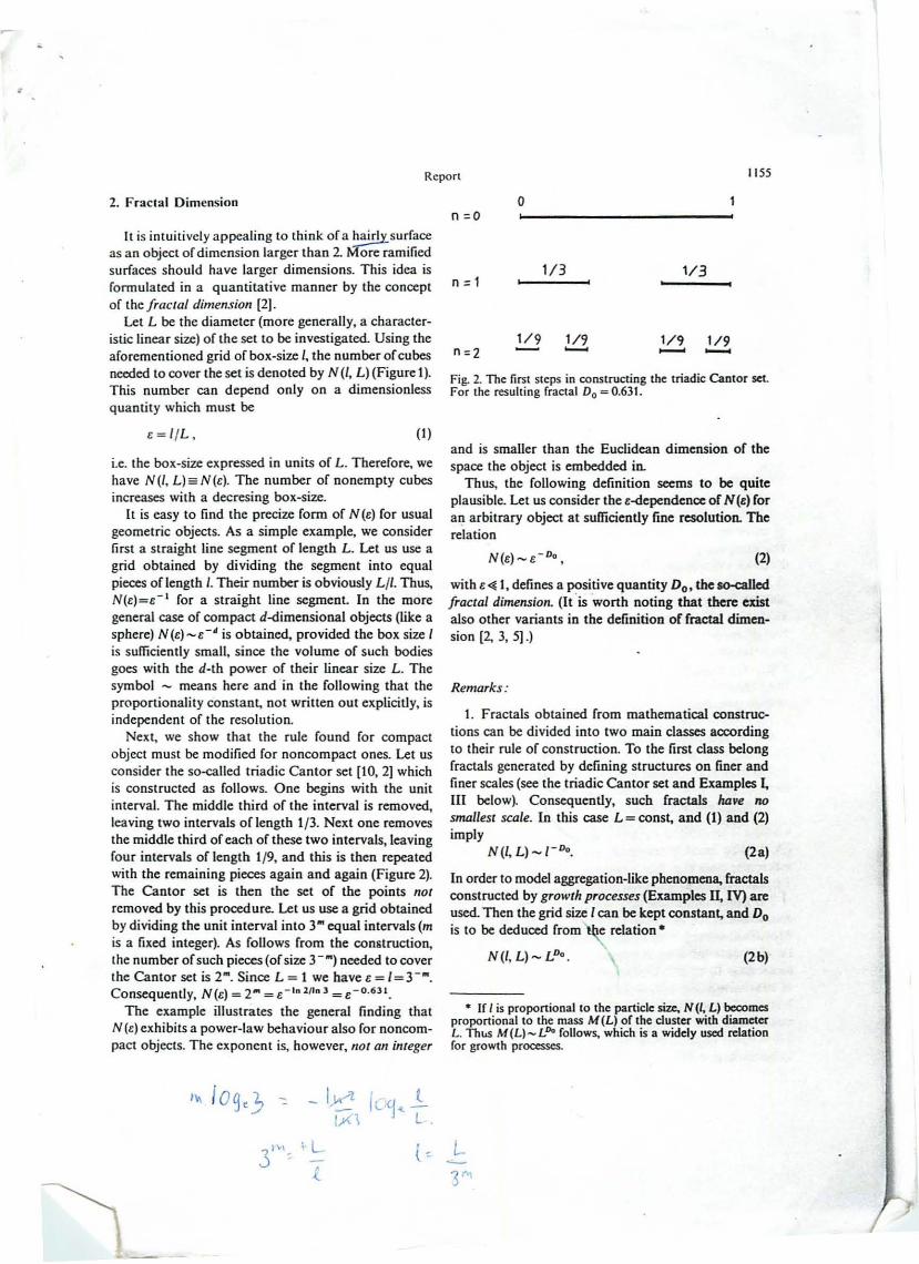
2. Fractal Dimensionn =0

o

Fig. 2. The first steps in constructing the triadic Cantor set.For the resulting fractal Do = 0.631.

II is intuitively appealing to think of a h~sur.face

as an object of dimension larger than 2. r-;{Qre ramifiedsurfaces should have larger dimensions. This idea isfonnulated in a quantitative manner by the conceptof the fractal dimension [2].

Let L be the diameter (more generally, a character­istic linear size) of the set to be investigated.. Using theaforementioned grid of box-size I, the number ofcubesneeded to cover the set is denoted by N (I, L) (Figure I).This number can depend only on a dimensionlessquantity which must be

n =1

1/9

1/3

1/9-

1/3

1/9 1/9.......... -

i.e. the box-size expressed in units of L. Tberefore, wehave N(/, L)=N(t). The number of nonempty cubesincreases with a decresing box-size.

It is easy to find the precize fonn of N(t) for usualgeometric objects. As a simple example, we considerfirst a straight line segment of lengtb L. Let us use agrid obtained by dividing tbe segment into equalpieces of length I. Their number is obviously LII. Thus,N(t)=t- 1 for a straight line segment. In the moregeneral case of compact d-dimensiooal objects (like asphere) N(t)-e-' is obtained, provided the box size Iis sufficiently small, since the volume of such bodiesgoes with the doth power of their linear size L. Thesymbol - means here and in the following that theproportionality constan~ not written out explicitly, isindependent of the resolution.

Next, we show that the rule found for compactobject must be modified for noncompact ones. Let usconsider the so-called triadic Cantor set [10, 2] whichis constructed as follows, One begins with the unitinterval. The middle third of the interval is removed,leaving two intervals ortength 1/3. Next one removesthe middle third of each of these two intervals, leavingfour intervals of length 1/9. and this is then repeatedwith the remaining pieces again and again (Figure 2).The Cantor set is then the set of the points notremoved by this prooedure. Let us use a grid obtainedby dividing the unit interval into 3'" equal intervals (mis a fixed integer). As follows from the construction,the number of such pieces (of size 3 'M) needed to coverthe Cantor set is 2'". Since L = 1 we have £ = 1= 3-'".Consequently, N(e) = 2'" = e- 1n 211n J = £-0.6Jl.

The example illustrates the general finding thatN (e) exhibits a power-law behaviour also for noncom­pact objects. The exponent is, however. /lot an integer

Remarks:

• If I is proponional to the particle size. N(l•. L) ~mesproportional to the mass M(L) or the cluster Wlth dwneterL. ThhS M(L)_LPo follows., which is a widely used relationfor growth processes.

with e~ I, defines a positive quantity Do, !be so-calledfractal dimension. (It 'is ·worth noting that !bere existalso other variants in the definition or fractal dimen­sion (2, 3, 5] .)

(2)N(t)_t'D.,

and is smaller than the Euclidean dimension of thespace the object is embedded in.

Thus, tbe following definition seems to be quiteplausible. Let us consider the e-dependence of N(.) foran arbitrary object at sufficiently fine resolution. Therelation

1. Fractals obtained from mathematical construe-­tions can be divided into two main classes accordingto their rule of construction. To the first class belongfractals generated by defining structures on finer andfiner scales (see the triadic Cantor set and Examples I,III below). Consequently, sucb fraetals have nosmallest scale. In this case L = const, and (\) and (2)imply

N(I.L)_I- D•• (2a)

In order to model aggregation-like phenomena, fractalsconstructed by growth processes (Examples II, IV) areused. Then the grid size I can be kept constant, and Dois to be deduoed from t~ relation'

N(I, L) - e'. (2 b)

(\ )t = IlL,

,

1156 Report

4 14,Fig. 3. A lypical In N(,) vs. 1n(1/,) plOL

where ). is an arbitrary positive number, follows from(2). Among usual geometrical objects there are alsoselfsimilar ones (e.g. linc, plane) but they are simple.Fractals arc, thus, nontrivial seUsimilar objects.

The fractal dimension turned out to be a very goodcharacteristic of different structures in nature [2).Moreover, in certain cases Do proved to be universal,i.e. the same for a class of systems. In many cases(coast line: Do ~ 1.25, landscape: Do ~ 2.2) the originof this universality is not yet known, in other cases,however. (polymer coil: Do ~ 1.66, the region of active,nonlaminar now in fully developed turbulence: Do ~2.8-3.0) the physical reasons of the universality seemto be understood [2J.

The resulting fractals have no largest scale. By an ap­propriate rescaling of the linear size, however, thissecond class can be made equivalent to the first one.This is exactly the physical meaning of the fact thatthe number of nonempty cubes depends only on theratio£.

2. Since N (e) cannot be larger than the numberof cubes needed to fill the space, Do;;; d is obtained.For compact geometrical objects, (2) holds with theEuclidean dimension, Do =d.

3. It has been mentioned that e must be muchsmaller than unity in (2). In physical examples, thereexists also a lower cut-off for e since the fractal struc­ture is replaced by some other patterns when ap­proaching the microscopic scales. Therefore, a straightline in the In N(e) vs. In (I/e) diagram can be observedin a range of. only (Figure 3). This range must extendover several decades in order to imply the existence ofa fractal structure.

4. Fractals arc selfsimilar objects, i.e. they look thesame on many different scales in the range where (2)holds. This is consistent with the fact that a scalingform

Do In 1/£. const

(5)V(n - V(O) - L'-' f7

has been found [2, II, 12J, where y>O is a new expo­nent(not a dimension!) and V(O) is the finite limitingvalue of the ohserved volume obtained for I~ O. Suchohjects are also fractals. These fractals are called foe[11 Jsince their d-dimensionaJ volume is nonzero.

A simple analytically tractabie example is obtainedhy modifying the construction of the triadic Cantorset in such a way [11] that, at the n-th stage, thefraction of each interval removed is (1/3)", rather than1/3 (e.g. at the second stage the middle ninth of eachinterval is removed).

Fat fractals are also common in nature. Examplesinclude [2) the vascular system, the branching struc­ture of bronchia in the lung, river networks, and thetop of certain trees which are with a very good accu­racy space filling ohjects.

In what follows we shall mainly deal with thinfractals.

The aim of this report is to give a tutorial introduc­tion to help new-comers from different fields of scienceto learn recent notions and concepts related to fractals.For tbis reason, mainly mathematical examples withsimple recurrent structures will be used which are bestsuited for clarifying concepts like multifractality orthermodynamical formalism. Nevertheless, the generalresults and relations we obtain hold for all fractalohjects. The article is not intended to be a historicalsurveyor a complete review of the field, as re"ectedalso in the choice of references which are concentratedonly on a few phenomena mentioned in the paper.Even these selections are necessarily incomplete, butthe author hopes they are sufficient to help the readerin further orientation.

3. Thin Fractals - Fat Ff1lctals

If the fractal dimension Do of a set is smaller thanthe Euclidean dimension d, the ohserved volume

V(n = N(e) I' - LD'I'-o, (4)

depends, actually. on the grid size I in the range where(2) holds. Such system are, therefore, fractals. We callthem thin fractals since V(Q would vanish in the limitI~ O. Such fractals are, in a mathematical sense, ob­jects of measure zero in the d-dimensional space.

It is worth mentioning that Do = d does not neces­sarily imply that the object is a usual body. In severalcases a power law behaviour

(3)

L-~ ln11£

N().e) =). -D. N(e) ,

InN(&)

Fig. 4. Schematic construction of a one-scale fractal.

o~I, '-. r

N(6)

1157

N(e) = NN,(e).

is obtained. which is an exact result for one-scalefractals [2].

Due to the similarity, Nt (e) is the same as the numberof boxes needed to cover the complete set with boxesof size Ilr:

N, (e) = N (elr) . (7)

By putting (6), (7), and (2) together,

In NDo = In (1Ir) (8)

Consequently, the fractal can be divided inlO Nidentical parts, each being rescaled versions. by a fac­lor r, of the complele set. Let N, (e) denote the numberof boxes on a grid of size /4 L (L is the diameter of thefractal) needed to cover one such part. Then the num­ber of boxes noeded to cover the complete fractal is

Report

rr r

ro

bl

<II

•

Cj

Fig. S. The flI'St steps in oonstructiDg a Koch curve (r = O.3~

The fractal dimension of the resulting fractal is Do =In 4/1n(ljO.3) = 1.151.

4. Deterministk Fractals

We study a few classes of fractals which are con­structed by deterministic rules. First, exactly selfsimi­lar objects possessing a recursive structure will be con­sidered.

One-Scale Fractals

The rule of construction for such fractals can beschematically represented as on Figure 4. One startswith a single object of linear size 10 , In the next stepthis object is divided into N identical pieces each ofwhich is a reduoed version of the original object by thesame factor r < I (hence the name one-scate fractal).The prooedure is then repeated in the next step so thatN of the newly created pieces of size 10 "> are arrangedinside a piece of size 10 r exactly in the same way asthese parts are arranged inside the original object(Fig. 4). The fractal is then obtained by applying thisrule subsequently ad infinitum.

Example I: Koch's Curve

The construction of a Koch curve [13, 2] proceedsas follows. Let us cut out from the unit interval tbeinterval (r,l-r), where 1/41i,.r~1/2 is a parameter.To the two newly created endpoints a V-shaped curveis added, both sides of which are straight and oflength r, as shown on Fig. 5a. The same process isrepeated with all sides of length r, and then again andagain (Fig. 5b, c) ad infinitum.

By comparing this rule with the general scheme wefind N = 4. The fractal dimension of a Koch curve istherefore Do = In 4/1n (1/r). It is worth noting that tbelength of this curve (tbe analogue of the surface area)diverges with the resolution: the length measured bybars oflength r-, m> 1 fixed, is 4-, as follows from tbeconstruction.

Example II: Snownake Fractal

The construction rule [14J shown in Fig. 6 can beconsidered as a model for aggregation processes. The"seed" configuration (n =0) is a symmetric cross builtby five particles. The configuration at the n-th slage isobtained by adding to the four corners ofthe(n-I)-thstage configuration the cluster corresponding to the(n-I)-th stage of the growth. By reducing the n-thstage configuration by a factor 3- one finds a series ofobjects of the same linear size [14]. The rule of con-

..

Fig. 6. The first steps in constructing a snowflake fractal witha growth process.

O@to lot) j=1.2 ..... N

Fig. 7. Schematic construction of a multi-scale fractal.

(9)

(10)

(11)/

N

N(e) = L Ni(e).i-'

From the similarity property,

Ni(e) = N (elr})

follows. Tbese relations and (2) then yield [2, 3)

which is an exact (implicit) equation for the dimensionof multi-scale fractals. For r, = ... = rN "" result (8)is, of course, recovered.

Report

procedure is then repeated in a similar way ad infini·tum (Figure 7). Consequently, the resulting fractal canbe divided into N parts, eacb being rescaled versionsof tbe complete fractal Let Ni(e) denote the number ofboxes on a grid (size 14 L) needed to cover the j·thsuch part. The number of boxes needed to cover tbecomplete fractal is

n:2

~ ..10

. .. 10. •.• •

• •o. 0

n=1

+n,O

1158

+

on=O

n:1 r; "{OJ {l}

,2 rtr2 Gr2 ,2n=2 1 ,

{OO} '1011 TiOi {;1J

Example III: Two-Scale Cantor Set

This fractal is obtained· by dividing the interval[0, I] as shown in Fig. 8 [16]. We initially replace tbeunit interval with two intervals of length r1 and r2

(r, +r2 < I). At the next stage of the construction thesame process is applied to each of tbese two intervals.Tbe procedure is tben repeated again and again. Tbegeneral formula (II) yields for tbe dimension

r," +rf' = I. (12)

Fig. 8. The first steps in constructing a two-scale Cantor set(r l = 0.25"2 = O.4~ For the resulting fractal Do = 0.61 1. Thecodes associated with the intervals will be explained inSection 14.

(Tbe ooe-scale Cantor set is obtained as the limitingcase r, =r2 =r. Then Do=ln 2/In(llr). For tbe triadicCantor set r= 1/3 and Do=0.631.)

5truction corresponds then to that represented inFig.4 with parameters N=5, r=1/3. Consequently,the dimension of the fractal is Do = In 51ln 3 = 1.465.

Mu/ri-Scale Fracrals

The essential dilference between the construction ofmulti-scale and one-scale fractals is the fact that thestaning object is now divided into N parts whicb arenor all identical. However, all of these are reducedversions of the original object by certain factors rJ< 1,j = I, .... N (all ri cannot be identical) [2, 15). Tbe

Example IV: Two-Scale Snowflake Fractal

Tbis is a generalization [17] of Example IL Tbe"seed" configuration is now a single particle. The con­figuration at tbe n-tb stage is obtained by adding tbetwice enlarged version of the cluster corresponding totbe (n -l)-tb stage of tbe growth to tbe four corners oftbe (n-I)-tb stage configuration (Figure 9). Reducingtbe object obtained after n steps by a factor 5' tbegeneral scbeme (Fig. 7) can be applied. Since r, = 1/5,r2 = ... =r,=2/5 we find

(13)

as an equation for Do- Its solution is Do = 1.601.

· -

-

~..<~

Fig. 9. The flf'St steps in constructing a two-scale ~nownake This function is more complicated than C(t) sin~ afractal by means of a growth process. scaling relation holds now only up to an additive

/

. smooth runction. For n~\);n-{~

W(yl) = y' -0 W(/) + cos (I) . (19)5. Fractal (unctions * ...........___

Consequently; the graph-or-W(I does have a largestThere exist eontinuous functions given by simple scale, W(/) has a maximum (Figure 11~

formulae, which are nowhere differentiable. The graph For the local rractal dimension of the graph, (17)of sucb a function turns out to be a fractal curve. has been shown to hold [21 J in the parameter rangeThese fractaJs are also deterministic ones. given by (15).

We consider, first, the Fourier series

the so-called Weierstrass-Mandelbrot function [2, 18J.In the range of parameters

(20)

(17)

1159

(X'(/) - I,

graph or C(/) has been shown (18) to be

0 0 =0

in the parameter range (15). As a runher eonsequenceor(16) the eurve C(/) possesses no sade 01 all, which isalso demonstrated on Figure 10.

The first example, or great historical importance, rora continuous but nowhere differentiable function wasgiven by Weierstrass (20). It is defined as

~ eas(y" I)W(/) = L 12-0'"' (18)

,,=0 'Y

where the bracket denotes averaging over severalrealizations. Relation (20), implies usual diffusion. The

6. Random Fractals

Fractals which are generated by nondeterministicrules are called random. In order to illustrate the dif­ference between the construction of deterministic andrandom fractals, let us eonsider the following example­In the first step of the deterministic eonstruction theupper right quaner of a square is cut out. Then thesame procedure is repeated in all remaining squares(Figure 12a). Modifying this rule by choosing sto­chastically which of the four quarters of th,e square inquestion is deleted, a random fractal is obtained(Figure 12 b). Although the geometrical appearance orthese two sets is quite different, their fractal dimen­sions coincide since the number of boxes needed tocover them is the same.

There exist also random fractal functions. The mostextensively studied phenomenon connected with themis diffusion or Brownian mOlion. The displacement x(/)of a Brownian particle moving along a line is a sto­chastic variable with zero average and with variance:

Report

(16)

(15)

(14)

n=2

.t.•••.·.·t..·•+.+••••

1- eos(y" I)

.- -00

n=1

C(/) '" L

1<0<2, y> I,

•

n=O

C (I) is eontinuous but the series defining dC(/)/dl di­verges everywhere.

By a formal replacement n _ n + I the scaling rela­tion

follows from (14) with y > O. Consequently, the graphof C(/) on the interval 10~/~y/o, 10 arbitrary, canbe obtained by magnirying the graph in the rangeleJy~ I ~10 with factors y and y' - 0 in horizontal andvertical directions, respectively. This nontrivial sym­melIy, the so-called self-affUlily [2, 19], can clearly beobserved in Figure 10. The fractal dimension" orthe

• Sections S. 6 provide an outlook on certain importantfields of fractals but can be omitted when reading the paperas an introduction to the subject of multifractals.

•• For self-affine sets a nontrivial fractal dimension. calledthe local dimension, can be obtained only by using a very finegrid. On long scales, (2) yields a trivial integer value (in ourcase unily) for Do [19, 9J.

r

(22)

Fig. to. The, Weierstrass-Mandelbrot function forD = J.5. y = 2. The plot was obtained by keepingFourier components with Inl~ 10 in (14).

Do=2-H.

7. Fractal Dimension for Composite Fractals

correlations extend to arbitrarily long time scales andhave a large effect on tbe visual appearance of thetraces (Figure 13). The graphs are self-affine fractalcurves with a local fractal dimension [2, 22]

Fig. 11. The Weierstrass (unction for D "'" I.S.1 = 2when it is 2x-periodic.. The plot was obtained bykeeping Fourier components with n:;; 10 in (18).

. ~Note that the fractal -dimensions of the curves2'" shown on Figs. 10 and 11 are the same.

Several fractals proved to be composite, i.e. to beunions of fractal subsets. Let us assume that a com-

Fractional Brownian motion is used when makingcomputer simulations of fractals like mountainousterrains or clouds [2, 22J.

Fractals in nature are typically random ones. Thefield of applications in physics is also extremely broadand ranges from percolation [23] and pattern/ormationthrough growth processes [4, 5, 24, 25] to chaos [26]and turbulence [2, 27, 28).

Despite this great practical relevance we sball, inwhat follows, mainly be interested in deterministicfractals which are best suited for an elementary intro­duction of further new concepts.

Report

(21 )

.,.

<x'(t) _ r'H ,

5 r------------------,

o

~~-------------,

aph of x(t) was proved [2, 22J to be a fractal curveth local fractal dimension Do = 1.5 (Figure 13 b).The fractional Brownian motion [2, 22J is an exten­In of the concept of the usual Brownian motion. The;placement x(t) of a particle following such a mo­n in one dimension is - by definition - a stochasticriable with zero average and with variance

ere 0< H < l. For H *' 1/2 this corresponds to anlmalous diffusion with correlated increments. Such

g. 12. Deterministic fractal (a) and a random version (b)it. The objects are exhibited here as obtained after five

:ps ofconstruction. The fractal dimension is for both cases,= 103/10 t =1.585.

Will

Cltl

1160

I',..

X II I

I

Report

laIH=O.2

D,=1.8

(bIH=O.5

D,=1.5

(clH--o.8

0,=1.2

J 161

Fig. 13, Traces of fractional Brownian motionat three different values of the parameter H(after [22)).

On the right band side the contribution with thelargest V\:' dominates for • ~ 0, thus, from (2)

plete set of linear size L consists of m fractal subsets,and let N.(.)" = IlL, denote the number of boxes ofsize I needed to cover the k-th subset on a grid. Forsmall box size Nk(e) - e - Db"', where D~) is the fractaldimension of the subset. Since the overlap among dif­ferent covers vanishes with decreasing box size, thenumber of boxes needed to cover the complete set is

The fractal dimension of the complete set is the sameas the largest dimension of the subsets.

This relation tells us that simple and completei fractals cannot be distinguished by measuring tbe

\

fractal dimension alone. Consequently, a more detailleddescription of fractals requires the introduction of fur­ther parameters characterizing different subfractals,How this can be done will be discussed in the nextsections.

~

N(e) = L N.(.).'-1

Do = max D~).

(23)

(24)

on the physical system in question. Here we mentiononly a few examples. On random resistor networks[29] the voltage or current distribution can be mea·sured. For aggregation processes the probability thata given site is the next to grow, the sCH:alled growthprobability, gives a distribution [30, 31). In the case offully developed turbulence the velocity dijJereMe in­side eddies is a quantity defining a measure [27, 28J. Itis to be noted that dilferent distributions may exist ona fractal leading to the existence of different fractalmeasures on the same support.

It is a recent observation [27, 32, 30, 16] that non·trivial distributions can be considered as analyse", ofstrange sets. They open up dijJerent fractal subsets bye.g. selecting subsets giving the dominating contribu­tions to different moments of the distributions. If thisis the case, the system will be called multifractal [32, 30,16, 33]. Different distributions may lead to differentmultifractal properties. It may happen that a fractalwith a given measure is a multifractal but with anoth­er one it is not.

The following simple example illustrates how anontrivial distribution selects different fractal subsetsof its support.

-

II. Multifraetals

8. Fractal MCllSUres

In several phenomena fractals appear not only asstrange geometrical objects but provide stages onwhich ·something is going on". Physical proCesses onfractals may generate stationary distributions (mea­sures). Fractals with time independent distribution onthem are called fractal measures (for a quantitativedefinition see the end of Section H~ The quantitywhich may be distributed on a given fractal depends

9. An Example for Moltifractals

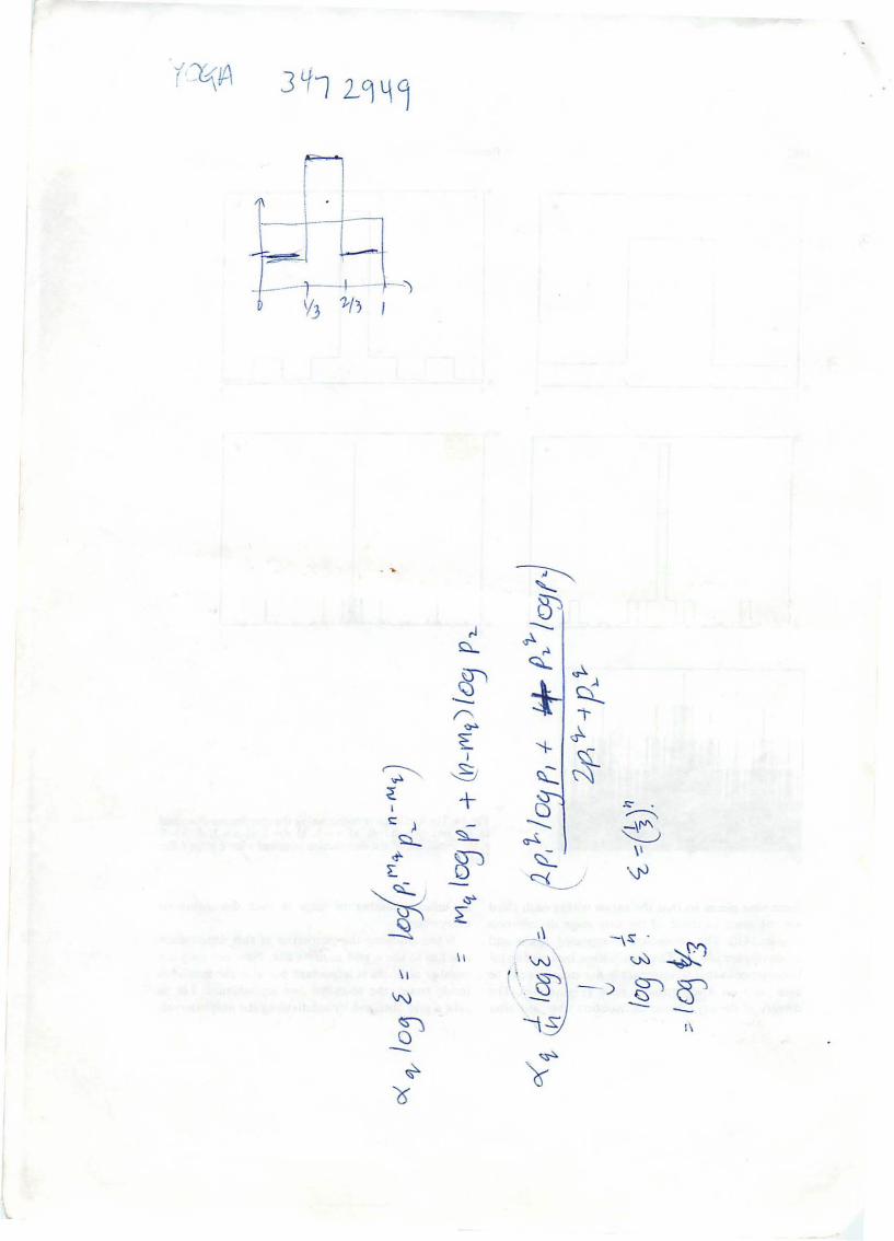
We consider here a probability distribution on theunit interval constructed by a simple rule [34J. In thefi",t step the middle third of the interval is made more(or less) probable than the outer thirds. Let the proba­bility of each of these pieces be PI' and the probabilitynf the middle third be P, = 1-2p, (Figure 14a~ Inthe next step each piece is divided again into thirds,and the probability is redistributed whithin each of

-

1162

'r----~----~---___,

•

l(i-lp.)

00L--:r,------.L------"------~

",------------------,c

Report

6r--------------...,b

o~=-==----==.--==lo

d

o I'

Fig. 14. The first steps in constructing the distribution describedin the text (P, =O.1l4~ a) "= I. b) "= 2, c) "- 3, d) "- 6,e) the logarithm of the distribution obtained after 6 steps (after[34)).

these nine pieces so tbat tbe ratios within eatb thirdare the same as those of the first stage distribution(Figure 14b). The procedure is repeated again andagain (Figure 140, d). The distribution becomes so in­homogeneous that its internal regular structure can beseen only on a logarithmic scale (Figure 14e). Thedensity of the asymptotic distribution obtained after

an infinite number of sleps is Iben discontinuouseverywhere.

When studying Ibe properties of this distributionone bas 10 use a grid of finite size. Now not only !benumber of boxes is importanl bUI also Ibe measuresinside boxes, tbe so-called box probabilities. Let ustake a grid obtained by subdividing Ibe unit intervals

~"-51---rJ

.A,.,~

~"'\'..l

~ I.:::l...- "t" J..0.>

~ '{..

~I

cC~ ~

.<c~ + CJ ~I

--- ~<:: ) -

<r.i..II

'SL~

SJ ~ \]'l<f-

~----.../r.

~ ""~1\ -IS" .

~

~r

W

---0.

\ , W

~cr" .8' -)

\ I

- - -"'l

"--lS II~~-

"a~

0

Report I J63

Their number increases again exponentially with n.We can, therefore, write

into intervals (boxes) of size I = <= (1/3)' with n ~ I. Itfollows from the construction described above thatthe box probabilities can take on one of the values

(25)

where m is an integer between 0 and n. Since thenumber of boxes 3" ~ n. there must be a degeneracy inthe distribution:

with Pm" are found to dominate, where

mq = 2p1n 2p1+p~·

(30)

(31)

i.e. these boxes cover a fractal subset of the unit inter­val, and I, is the dimension of this subset From(26)-(28)

~,

f1 (note that mIn is a quasi continuous quantity forn ~ I).

The number Nm, of the relevant boxes increases, ofcourse, exponentially with n. Since the resolution is<= (1/3)', N~, can be written as

(32)

In(2pj +p'l)J In(~/3) /

This means that a subset offractal dimension h, givesthe dominant contribution to the sum of the q-thpower 01 the box probablities. Note that for q'!' I thissubset is dilferent from that contributing to the totalmeasure. In our example

is obtained as can be checked easily.By increasing (decreasing) the exponent q, boxes

with higher (lower) probabilities, i.e. fractal regionswith denser (mor!:rarified) occupation are selected. Infact, the limit q~ <Xl picks up the most probable boxwhich is alone. Consequently, 1m = O. The oppositelimit selects Ihe least probable boxes. Their number is2', therefore I-m = In 2/1n 3. ,esc limiting resultscan be obtained also from (32).

We have, thus, demonstrated that the contributionof the 'sum of different powers of the box probabilitiesis dominated by different fractal subsets. The spectrumI q of their fractal dimension provides a characteristicof this multi/ractal. The example also illustrates thatan inhomogeneous distribution on a non..jractal sup­port (here the unit interval) can be multifractal.

In addition to the fractal dimension also the contentof those boxes which contribute, i.e. the probabilityp... belonging 10 each of them, is an important quanti.ty. Since, however, p... depends on n (or eJ, it is betterto introduce an e~independentparameter, the crowd­ing index tIq , by writing

_[2 pj In pI +1'1 In 1'11,- 2pl+p'l

(26)

(27)

(28)

v·

is the number of boxes with the same measure P",. Forthe sake of definitness we assume P2 > PI"

First, we ask which boxes give the main contribu~

tion to the total probability when refining the grid.Although the most probable box is that in the middle,with content Po =Pi,.Jl is alan . Its contribution isnegligible for n ~as since pz 1. The most rarified

......-boxes (P" = pi) are 'nlLmerOl!S; evertheless the proba­bility in such boxes is also negligible since (2p,J" ~ o.It is, therefore, plausible that, for large n, columns veryclose to some medium hight give the main contribu­tion. More precisely, for n - 00 there exists a singleindex m = m, (n) between aand n, so that only boxeswith p... contribute to the total probability: NM, P"" -1.Consequently, none of the other boxes are importantfrom the point of view of the total measure. An easycalculation (see Appendix) yields

f _ 2p, Inpi +pzlnpz,- In 1/3 (29)

P.... =e..".

From (25) and (30)

(33)

is obtained. 2pj In p, +1'1 In pz 1Next, we investigate the q-th poweroflhe box prob- a, = 2pj +1'1 In(I/3) (34)

abilities. where - co <q < 00 is a parameter. The total / . .amount of these quantities is L N 1" = (2pj +pj)" Jis found. The values of a, lie In the range between

m ~ ~ 'z· am = InpJln(1/3) and a_m=lnptlln(I/3~(For theSimilarly to the previous case, columns of a certain particular choice ofp, used in constructing Figs. 14-17height contribute only to this sum. At a fixed q, boxes (P, = 0.1 14) we "btain am = 0.234 and a_ m= 1.981.)

Report

(37)

(38)~-e~.

i.e. these boxes cover a subset of fractal dimensionf(a). The variable a may take on values from '!-@Dge[a~, a_~l, and f(a) turns out to be, in ieneralJasingle humped function with Do as its~um [16](Figure 16). The f(a) spectrum of a simple lctal con­sists of a single point.

where a is position dependent Relation (38) definesthe set of crowding indices [16) (or Holder exponents[2)) a. At any fixed • there exis~ however, severalboxes with a given crowding index, say. a:.. Their num­ber N.(e) increases witb e like

N.(.)_e-f(·', (39)

proximately a constant, ~. The crowding index a" forthese boxes is defined by the asymptotic relation

o d._

o

fllI-f( J. I ~,

/\'--:\ -;

L--.\ )'"

Fig. J6. The I(a} spectrum for the multifractaJ of Sect. 9 asobtained from (32) and (34) by eliminating q. The straight lineis the diagonal f = a.

A multifractal is then characterized by the spectra I.and «".

Since Xo(') = N(.), the quantity fo is tbe fractaldimension Do of the support. It follows from the prop­erty of composite fractals (Section 7) tbat fo>J. forq '" 0 since the multifractal is tbe union of all sub­fractals with dimension f,. The function I. vs. q in­creases until it rcaches its maximum Do and then de~

creases. As higher powers select denser regions., IX" ismonotonously decreasing (see Figure 15).

A simple fractal corresponds in this picture to thespecial~...

The eliminatIon of the variable q between I. and a,leads to a new characteristic, to the so-<:alled f(a)spectrum (16). Direct definitions of a and f(a) can begiven as follows. For £-+0 around each point of thefractal one finds

(35)x,(I, L) '" L P;' ,

0.5

-r---=o-;:---------, 2 1.5 r------r--,

---

The spectra I. and a, are exhibited in Fig. 15 for acase P2 > PI' Note that the multifractal properties arelost for the parameter values PI =P2 = 1/3 whenJ:, = all = 1, since the density is then constant over thewhole intervaL A similar case is obtained for P2 = 0,PI = 1/2 when I. = a, = In 2/ln 3. This correspondsjothe familiar triadic Cantor set with a uniform dislji6u-tion on it. t//

~10. Characterization of General Multifractals

where J. is the fractal dimension of the subset. Fur­thennore. the content of each contributing box is ap-

'-------------"'~-+o

the sum over all boxes of the q-th power of the boxprobabilities, - 00 < q < 00. X, depends only on thedimensionless number e == IIL. where L is the linearsize of the support: X,O, L) =X,(.). For q =0, (35)yields the number of boxes needed to cover the sup­port. Since the distribution should be normalized,Xd') '" I holds.

The properties of the previous example turn out tobe typical for multifractals. For e -+0 the contributionto X,(.) with a given q comes from a subset of allpossible boxes. These boxes cover a fractal, I.e. tbeirnumber N,(') depends on • as

N,(') -.- f. , (36)

In order to describe multifractal properties a uni­form grid of size I, as introduced in Section I. is usedagain. Let P; denote the measure or probability insidetbe i-tb box: for empty boxes Po vanishes. A centralquantity [35, 15,36) is

-4 0 q. 4

Fig. 15. The q-depcndencc of the fractal dimension ~. (32),and of the crowding index IX., (34), for the multifractal con­structed in the previous Figure.

b~c;dJoe k(I~I'I

Ij n

, 0

J Pkq,.I v

11'\ I

n +OoJ

fJvII ""( X\ Yt <Ii 'AVbWC

< dI) e1- I,

e, oj

Report

Before turning to the question how a" and f., can be 0... .,-----------------.obtained from f(a.) it is worth introducing the conceptof generalized dime~sions.

0,

II. Generalized Dimensions

1\65

(43)

- L P, In p, - D, In (I/e) .I

The quantity X,(£) is ~otind to follow a power lawbehaviour as e - 0:

(40)

where 0 q is the so-called order q generalized dimension[35, 27, IS, 36). The faclOr (q -I) has been pulled outin the exponent to ensure automatically the relationX, (£)= I. Consequently, the D;s are positive numbers.Thcir values monotonously decrease with q [15J(Figure 17). For simple fractals all the D;s coincide.

It is easy now to connect the generalized dimen­sions and the spectra /4' a". Since the contributionto X,(£) is given by boxes with content P, we haveX,(£) = N,(e) p;. This implies via (36), (37) and (40)

(q-I) D, = q a,-I,. (41)

For q = 0 the relation Do = fo is recovered. Further­more. as /q is finite, D ± co =a: ± OD follows.

In order to find the relation to the f(a) spectrum letus notice that X,(£) can be written (see (35), (38), (39))for e-0 as " -,

X,(e) - J£" - [(., da, ) (42)

when a is a quasi~c6ifiinuous variable. Since E is verysmall, the integral will be dominated by the value of awhich makes the exponent minimal. This immediatelylead~ to (41) with the conditions

df(a) I = q',d f, =f(a,).a ",

!X4

is, therefore, that particular value of the crowdingindex for which the derivative of f(a) is exactly q.As a consequence, also the spectra f(a) and (I-q) D,are connected: they are Legendre transforms of eachother (see (41)).

The case of the order I generalized dimension is ofspecial importance. From (41) and its derivative takenat q = I we find

(44)

This relation together with (43) explains why the I,and a, curves touch each other at q = I (Fig. IS) and

----4­D_o 0

-10 0 q 10

Fig. 17. The D. spectrum for the multifractal of SectiOD 9.

why f(a) is tangent to the diagonal exactly at a pointwhere f(a) = a = D, (Figure 16). Furthermore, by per­forming the limit q _I in (35) and (40) one obtains

(45) IIIThe quantity D, thus measures how the information(left hand side) scales with In(l/e~ Therefore D, hasbeen called the information dimensio.n [37, 34]. More­over, this concept has been used to give a precisedefinitio. ·Jf fractal·measures [34): a distribution issaid to b" a fractal measure if its fractal dimensionexceeds its information dimension. In this sense theexample of Sect 9 is a fractal measure and, moreover,all fractal measures are multifractals. (The value ofp,used in Fig. 14 was chosen in such a way thatDI = In 2/ln 3, i.e. the same as thefractal dimension ofthe triadic Cantor set The fractal dimension of thesupport is, of course, unity in this example.)

It is worth noting that despite their name, the gener­alized dimensions D, (q'i'O, I) are not dimensions. asexpressed by (41). This can also be seen from the factthat all D, with a negative q are in the example ofSect 9 larger than 1 (Fig. 1~ Nevertheless, the spectraDq and f(a) (or I, and a,) provide equivalent charac­terizations of multifractals. (For another interpretationof D, see [27].)

Finally, we mention that distributions on fat frac­tals can also be multifractals characterized not only byD, but by another set of exponents r. obtained bygeneralizing (5) [38).

12. Fractals Measures ..ith an Exact RecursiveStructure

The class of fractal measures possessing an exactrecursive structure provides analytically tractable

I~

Fractals on which a measure is distributed with aconstant density form an interesting class, since insuch cases multifractality. if present., manifests purelygeometrical properties. The multifractal spectra canthen be considered to characterize the fractal supportitself. An example is provided by tbe two-scale Cantorset of Sect. 4 if tbe measure associated witb an intervalappearing in tbe construction (Fig. 8) is cbosen to beproportional to the lengtb of the interval (to theLebesgue measure). Multifractal properties then re­flect the heterogeneity in the size-distribution of theseintervals.

Such geometrical multi/ractality [17] is of specialimportance for growing structures, where a distribu·tion of constant density always exists and is of pbys­ical relevance. This is due to tbe fact tbat such systemsare built up by identical particles and, therefore, themass distribution on the growing structure is uniform.The multifractal properties witb respect to this mea­sure can be analysed along tbe lines described inSect. 10 by cbosing tbe box probability Il to be pro­portional to tbe mass, or tbe number of particles,inside box i.

As an example, let us consider the two-scale snow­(fake fractal of Section 4. By reducing the object ob­tained after n steps of construction by a factor S· thegeneral scheme worked out in the previous Sectioncan be applied The cluster consists of a smaller cen­tral and four larger pieces eacb baving tbe overallshape of a square (Figure 9). Since tbe masses of thesedifferent sqaures are 1/17 and 4/17 parts of the totalmass, one obtains [17] from (48)

(47)

(48)

(46)

/

"X,(e) = L X,.;!t).J= I

From these relations and from (40)

follows, where x,je) stands for the quantity definedby (35), evaluated for the j-th piece by using a grid ofsize I (e = IlL, L is the linear size of tbe support). Forthe complete system

is obtained, which is an exact equation for the general­ized dimension D, [15]. For q =0, of course, (II) isrecovered.

If the support is a one-scale object, i.e. if'j = r for allj, the implicit" equation (48) can be solved, yielding

1166 Report

/

cases. \Vc consider measures for which the rule of 13. Geometrical Multifractalityconstruction is based on that of multi-scale fractals(Section 4, Fig. 7). Now the redislribution of the mea­sure is also to be defined. Let Pi be the probabilityassociated with the j-th piece which is the reduced

"version of the original one by a factor 'j. L Pi = 1. Atj=1

the next stage of construction each piece is furtherdivided into N pieces, each with a probability reducedby a factor Pi and size by a factor 'j. etc. The supportof the resulting measure can, therefore, be divided intoN parts, each being a rescaled version of the completesupport, by a factor Tjo Each such part carries anamount Pi of the total measure. From this similarityproperty

./

(50)I In (f PJ)

D = ~J_'..:.I--,:...

, q - I In r (49) The D, values lie in the range between D~=ln(17/4)1In (5/2) = 1.579 and D _~ = In 17/1n 5 = 1.760. The

This result applies also to tbe example of Sect. 9, numbers appearing in (50) are linear size and areawhere N = 3, r = 1/3 and PI = p,. ratios of the five main squares, with respect to the data

Note that in cases wben the probability is dis- of the whole cluster, which reflects the fact that thelributed uniformly on a one-scale support (Pj= liN), multifractality is in tbis case of geometrical origin.multifractal properties are lost since D4 == a4 =/4" It is worth mentioning that a growing structure= In N/ln(l/r) for all q. For measures on multi-scale may be a multi fractal, say, witb respect to the growtbfractal supports, tho property of multifractality is probability and, simultaneously, a geometrical multi­more persistent. Even a uniform distribution of the fractal~ i.e. a multifractaI.. with respect to the homoge-

probability, i.e. the choice p = r.!( f r), leads to a neous mass distribution on the structure. The spectra} J j=1 j) lR\ / for these two multifractals are then, of course, differ-

nontrivial D q spectrum, as can be seen from (~ 'ent.

/

- f,nj lAp WYI5u/Cl,f-t _- P~l> i?0 u:e ----- GClUI (, e-

-- vJtV( re<! (h (jet~

..... ;; .: -' .

RcpOrl 1167

(52)

15. Statistical Analogy - Thermodynamical Poteatials

wbere Ko is an important characteristic, the topole>­glcal entropy [26) of the hierarchy. On a k-nary trceKo ~ In k, where the equality holds for a trivial gram­mar when the number of allowed sequences is just k". ./

Unfortunately, there is no general recipe for encod­ing a hierarcby. Only intuition'and a detailed knowl­edge of the particular physical process ntight help tofind the encoding of the fractal generated.

In what follows we assume that the encoding hasbeen found. Let S,S2 ... S."'{s,}",SJ denote a codeoccurring at the n-th stage of tbe hierarcby, where theelements s. can take on values 0, 1, ... , k-l, andJ = I, ... , W(n) is a subscript specifying the code. Toeach code there is a box covering tbe part of the fractalwhich is associated with that particular code. In con­trast to boxes of a uniform grid, these boxes fit to thefractal structure in a natural way providing an "opti­mal" coverage. For the sake of simplicity we assumethat the boxes are d-dimensional cubes where d is thedimension of the space the fractal is embedded in. (Anextension for more general cases can also be workedout.) The size of the cube associated with a code SJ isdenoted by /J '" I(s;}). Let eJ '" e({s,ll = IJIL repre­sent the length scales measured in units of the diame­ter L of the fractal. It is worth introducing [41, 47] fora given code of length n the quantity

14. Encoding

Fractals are. in general, organized in a hierarchicalway which is often reflected in their rules of construc­tion. Tbe fact that this hierarchy can be encoded is thebasis for the thermodynamical formalism. To illus­trate the concept of encoding. let us take again a sim­ple example: the two-scale Cantor set of Sect. 4 (seeFigure 8). The number of intervals used to approachthe fractal doubles in each step, thus, at the n-th stageof construction there are 2" intervals. Each of themcan, therefore, be denoted by a binary number oflength n. Let us apply the following rule: At the firststage the intervals of length r t and r 2 are associatedwith the symbols 0 and I, respectively. In general, thelast digit of the code for "daughter" intervals is 0 or 1depending on whether their length were obtained by

/"

The thermodynamical formalism has been workedout in mathematics for describing fractal properties ofchaotic dynamical systems [39]. It has recently beendeveloped into a powerful technique [40-46], acces­sible also to experimentalists, providing more accu­rate results for the multifractal properties than boxcounting methods described in the previous sections.The concept of thermodynamical potentials has al­ready been extended (47) for fractals which appearbeyond the scope of dynamical systems. Based onthese developments, we go here one step further andshow how the thermodynamical formalism, built onan underlying spin system, can be worked out for suchfractals. We shaH see that the thermodynamical poten­tials arising in the formalism give the most generalcharacterization of fractal and multifractal objects.

In the next sections we introduce the so-called ther- multiplying the Jength of their "mother" interval by r t

modynamical formalism, the importance of which in or r2 (Figure 8). Note that each code specifies ao inter­natural sciences has been realised only very recently. val uniquely, but there is a degeneracy io the length ofBesides providing a broad theoretical framework, us- the intervals.ing the language of classicaJ sta . tical mechanics, Several fractals can be encoded in a similar way.this method possesses also practical relevance since it The encoding consists of two important items: i) theyields more accurate results than a direct application "ABC": the number k of independent symbols needed,of the definitions of Chapts. I and Il. The formalism is and ii) the "grammar": the rules telling us which sym­expected to become a widely used characte/rizationof bol sequences are aHowed. In the previous example.fractals and multifractals in the near future. the grammar was trivial, all hinary sequences occurred.~ In general. however, this is oot the case and ocrtain

\ . sequences are to be excluded. Such hierarchies can~ Ill. The Thermodynamical Formalism for Fractals then be represented by a k-nary (binary, ternary, ... )""Jt' 'and Multifractals tree which in the case of nontrivial grammars is not

complete. Nevertheless, the number W(n) of elementsat the n-th level of the trce grows rapidly. For large n

W(n) - exp(Kon), (51)

I

I

1168 Report

where - 00 < P< 00, and the sum is taken over allallowed sequences of length n (n l> 1). We note by pass­ing thai exp {-pFljl) appears also as an eigenvalueof an operator which can explicitly be constructed forfractals organized on a k-nary tree [46]. I,

Two special values of PF(f!) follow immediatelyfrom (54). For P= a the sum is just the number ofallowed sequences, thus

(57 a)

(57 b)

Meaning in statistical mechanics

microstatenumber of spinsthermodynamic limitinverse t~ratureBoltzmann factorpartition sum

energy per spin (in a macrostate)number of microstatesemropy per spinfree energy per spin

dS/dE =p.where

p~ ~cxp(-pE,n)

L~,EWSF

code (Si}

Fractal characteristics

n

Relations (53) and (54) correspond to a microcanDn-ical and canDnical description, respectively. In the IL, see «lhermodynamical limit these ensembles are equiva- ~1 (,\iI.OJ"Jlent, consequently, PF(f!) llIId (-S(£) are Legendretransforms of each other, Le.

It is worth noting the parallelism between the pres­ent fonnalism and that of statistical mechanics. Thekey observation is that any allowed sequence {SI} canbe associated with a microstate of a chain of n. ingeneral interactive, spins (for k = 2 Ising mode~ other­wise k-stale Potts model). Thus, the analogy can besummarized as follows:

(53)/The spectrum S(£) characterizes lhe length scale dis­IribUlio1l of the fractal. The maximal value of S is, ofcourse, the topological enlropy K o (Fig. 18 a). mustra­live examples will be given below.

Another characteristic can be obtained by consider­ing the sum of lhe length scales raised to a power p.This sum changes with n also in an exponential fash­ion [41, 47J, i.e. we have-

Le1=LC'({Sill-e-m"., (54)J II1I

In the limit 11-00 the value of E is positive and liesgenerally in an interval (E_, E.) [41, 47J. In otherwords. the characteristic exponents E tell us howrapidly the length scales decrease with increasing n. As11 grows, there are. in the coverage. more and mOTC

boxes of the same size belonging to a given value of E.Their number W(n, E) increases exponentially [41, 47J,i.e. for large 11 ~e can write

W(n, £) - eSIE) ••

(55)

Fractals are asymR!0tically selfsimilar: the coverageobta\ned~he~-t~tevel is similar to that obtained atlhe (2 n-th )evel,1Or n l> I. The role of the similarityrati~efined in Sect. 4 (see Fig. 7) is then played justbe the t/5. A compari~~£Of (11) with rj = £j.

N = W(n), and (54) ShOWS'" /

PF(f!) I,-D, = o. J (56)

This means lhat the sum of the length scales raised toa power p remains finite in the n - 00 limit if P ischosen to be the fractal dimension. For fractals associ­ated with dynamical systems relation (56) is the so­called Bowen-Ruelle formula obtained in [3~J. (Strict­ly speaking, the particular P value for which F(f!)vanishes was proved to be the so-called Hausdorffdimension [2} which. however, coincides with Do dis­regarding very exotic examples.)

• The quantity (- PF (P)) is often called the pressure func­lion [39). We prefer to call F(fi) the free energy as followsfrom the statistical analogy (d. table in the next column).

They both decribe a new spectrum offractal properties.S(£) is typically a single humped function, while PF(f!)is monotonic increasing with a nonpositive secondderivative (Figure 18).

The quantity PF(f!) is a linear function for one-scalefractals only. Using (51) and (54) PF(f!) = PEo - K o isobtained, where Eo is the energy value characterizingall the boxes.

In the example of the two-scale Cantor set, thelength scales can be expressed as c({s,ll = r;' ri--,where m is the number of a's occurring in the (binary)code {soJ. This number uniquely specifies, via (52), anexponent E(m/n). Based on the fact that the multiplic­ity of intervals characterized by a given ratio min, or

E(m/n), isjust (:) = W(n, £), it is easy to check, using

(53) and (54), that (58)

E-E_ (E-E_) E.-E (E.-E)S(£)=---In -- ---In --tJE tJE tJE tJE'and

(59)

!

.Il.

z 5

InSa) K. f3F(Il) b)

0s(E1

1 ft GCB.p)

Report

-0

o /3'00 ....... / -2

/'

..···p=2 .-. / -3K.:>.

p=O / I./

// p=-2,..

1169

o . f2±-''''----'''------+--------10.8 LEE.1.7 - B 0 f3

Fig. 18. Thermodynamical properties for the two-scale snowflake fractal (Fig. 9). - a) The plot of the enlropy functionS(El= -{(E- E.)/"£] In (E - E.)/"£]-(E, - Ell"£] In (E. -El/l4"El), where"E = E. -E. and E. =0.916, E. = 1.609.b) The plot of the free energy (heavy line) PF(PJ = -In (4 (0.4)' +(0.2)'). For comparison also plots of the Gibbs potential (secSect. 16) are shown. The latter is taken with respect to a measure defined with an exact recursive structure, as described inSect. 12, on the two·scale snowflake fractal. Here the particular parameter values Pt =0.12, P2 =... =Ps =0.22 are chosen.Thus, PG(P, p) = -In (4(0.22)"(0.4)' + (0.12)' (0.2)'). Dotted and dash-dotted lines correspond to PGlP, p) at [lXed "pressure"p=2 and p= -2, respectively.

2..-----------,D.

2

Fig. 19. f(rt) spectra with respect to distributions (60) for thetwo-scale snowflake fractal The values q =0, 1,2 and 3 arctaken and the spectrum is obtained via (63). The case u = 2corresponds to the D" spectrum defined by (SO}. Note that forq = Do measure (60) is not a multifraetal since there existsthen a single index ::r =Do= 1.601 only (sec (56), (61)). Fora ..... Do the widths of the spectra tend to zero.

where E. = In (l{r2 ), E. = In (I{r,) and tJE = E. - E..Here we have assumed, without loss of generality, thatrz > r t . These results show that the thermodynamicalpotentials of the two-scale Cantor set are those of nnoninteractive two-state systems with energy levelsE_. E. (e.g. spins in magnetic field) [48). .

The two-scale snowflake fractal (Fig. 9) might seemto be a less trivial example. In this case the "ABC"must have 5 elements. but the fractal still shares thethennodynamics with n independent spins. They arenow 5-state spins~ the lowest energy level of which is4 times degenerared (E_ = In (5{2) = 0.916, E. = In 5 =1.609). It is recommended that the reader derive the

expressions for the potentials given in the caption toFigure 18.

In more general cases without exact recursive fea­ture the associated spin chain is interactive. Infiniterange interactions might lead to a qualitatively newphenomenon, to a phase transitian [49J reflected bynonanalyticities in the thermodynamical potentials.(A simple example is provided by a fractal the cover-age of which contains a single box with an exponentE., while all-other box sizes scale with another valueEo>E•. This leads to F(Jf)=E. for P>P, andpF(Jf)=pEo-Ko, otherwise. At P,=Ko{(Eo-E.) afirst order transition occurs.) A detailed discussion ofthe phenomenon is beyond the scope of this paper. Itis worth noting, however, tbat methods worked out tohandle phase transitions (like transfer matrix, finitesize scaling) can successfully be used also in the ther­modynamical description of fraetals [49]. while the Weigenvalue fonnalism mentioned after (54) provides anew lechnique [46, 44).

16. Relation to the MoItifractaJ Spectrum ­lhe Gibbs Potential

It is clear from the definition (52)-(54) that bothS(E) and F(Jf) reflect purely geometrical properties ofthefractal. They have, therefore, a priori nothing to dowith the multifraetal spectrum characterizing also adistribution on the fractal. For an important class offractal measures, however, flo) can be shown to beclosely related to S(E).

(

o~

1/70 Report

a is a parameter of the measure. The crowding index(38) for boxes with a certain value of E is thus

eOP

J", pels;}) = _J_ _ eo"ol.-oe,.. (60)

L/;~J

i.e. a unique function of E. The number of boxeswith a given a (or E) must behave as a power ofe=exp(-EII):

e S "" _ (e-e.)-n., (62)

(66)

(65)

(67)

pGp(P, p) 1"0 = (q-l) K •.p',

PGp(P,P)I'."-., D • =0P-'

which defines a new set of parameters, that of the K, 's.Using the terminology of dynamical systems, we callK. the order q generalized elltropy [50] with respect tothe distribution P. (The q = 0 case corresponds to thetopological entropy.) From (64) and (65)

- CO <q < <.0. Since the distribution PJ is normalized,the sum scales with II [SOl as

Thus, the spectra PF(p) and (P-I) K pare obtained asrestrictions of p Gp(ft, p) on two orthogonal axes p = 0and p= 0, respectively. To determine the multifractalspectrum some intermediate point of the p- p plane isneeded: Using again the fact that fraetals are asymp­totically selfsimilar and recalling (48) (with PJ=PJ'rJ=eJ, N = W(II)) we obtain

(63)

(61 )~ ~ a - a F(a)/E,

SeE) If(~)=E £_oF'a'

a-.

from which

Let us consider measures· with the following prop­erty: the probability inside a box is proportional to apower a of the box sire (- 00 <a < co) for all boxes[41,44,45]. By taking into account normalization thismeans

follows. [n such cases, therefore, the entropy [unctioJluniquely specifies the f(~) spectrum. Geometricalmultifractality as defined in Sect. 13 corresponds tothe choice a = d. Figure 19 exhibits the f(a) spectraobtained in this way for a few values of a in the caseof the snowflake fractal shown on Figure 9.

When the probabilty of a box depends on the sizein a more complicated way than power law, SeE) is nolonger related to f(~) in any simple manner. It isthen worth including also powers of the probabililiesP; '" P({s,}). i.e. the measures of boxes specified by (sil,into a partition sum (16, 36,43,47]. Let us consider

L. P! ~ = L. PP«si})e'«si}) - e-,G.".pl., (64)J lli1

as an implicit equation for the spectrum of generalizeddimensions D. with respect to the measure P. Equa­tions (66), (67) are extensions of (55), (56). They meanthat D. and K. can be obtained from the plotp Gp(fJ, q) vs. Pby cutting it with the horizontal andvertical axes, respectively. In view of this, the twoimportant spectra D. and K. appear only as partialcharacterizations of a fractal measure, a much richerdescription of which is given by the Gibbs potentialGp(fJ, p) itself. Figure 18 b shows also plots of the p0­

tential P Gp(ft, p) at f",ed values p for a distributionhaving an exact recursive structure, as defined 10

Sect 12, on the two-scale snowflake fractalIt is worth noting that for measures of type (60)

pGp(fJ, p) = (fJ +ap) F(ft+a p) - a p F(u), (68)

i.e. all quantities can be expressed in terms of the freeenergy alone.

Distributions on one-scale fraetal supports fromanother interesting special class. Such cases are char­acterized by a single energy value Eo, and consequently

where - 00 <p < 00. In the language of statisticalmechanics this is the analogue of an isolerm-isobarensemble [48]. The parameter p is the "pressure", -In 1]plays the role of a nuctuating volume divided by thetemperature, and Gp(ft, p) represents the Gibbs potell­lia/ per spin. The subscript P is to remind us that thepotential now depends on the dislrihwion.

The free energy is recovered from the Gibbspotential for p = O. A completely dilTerent charac­teristic of purely probabilistic nature is the sum L: pt.

J

and

P F(p) 1'-lI-.,D....=qa F(a),

aqK. ~ q"': 1 (F(aq) - F(a)),

(69 a)

(69 b)

• Called Gibbs measures in dynamical systems (391. pGp(fJ, p) ~ P Eo + (p-l) K p, (70)

/

i.e. the plot PG,(fi, p) vs. Pis a staight line for all fixedp. From (67) the explicit relation Eo D, = K, followsthen between dimensions and entropies. The exampleof Sect. 9 belongs to this class with Eo = In 3.

Finally, we mention that there is an essential differ­ence in calculating the multifractal spectrum via (39),(40) and via the thermodynamical formalism. Whenintroducing D, and J(a) we used a uniform grid. Theorganization of the fractaL however, defines a range oflength scales and a coverage of the set by boxes ojdifferent size. This is why the equations specifying themultifractal spectrum appear now in different forms.The knowledge of the encoding helps to find an "op­timal" coverage which is optimal also in the sense thatthe asymptotic regime in n is reached for this coveragemuch faster than by refining a uniform grid. In otherwords, the application of the thermodynamical for­malism provides an increased precision in describingthe scaling properties of multifractals. In particular,this is the case at phase transition points, which arevery difficult to locate by means of other methods.

IV. Closing Remarks

Although it is not been the aim of this report to givea complete overview of what has been done on thefield of fractals and multifractals, it is worth illustrat­ing the wide range of recent applications in naturalphenomena by few examples. We do not go into adetailed discussion of the results since many of themhave recently been reviewed [51, 52, 8, 9]. Rather wegive here a pictorial comparison of J(a) spectra ob­tained for different systems in numerical or laboratoryexperiments (Fig. 20) [52-56).

[n the case of chaolic motion the most importantdistribution on strange attractors is the so-<:aIIed nat­ural measure [26), the distrihution descrihing howoften a given part of the attractor is visited by chaotictrajectories, in the long time IimiL This defines afractal measure, which under special conditions [40,41,44,45] can be also of type (60). The field of dynam­ical systems is the one where the thermodynamicalformalism has successfully been applied. Recent for-

/

1112 Reporl

Of

mulations arc based on the sel of all unstable periodicorbits [57. 531 which can uniquely be encoded. Phasetransitions have been found to be typical for chaotica!tractors [49J. Figure 20a exhibits the f(a) spectrumfor the Henon attractor. in which a straight line seg­ment, the sign of a phase transition. can clearly be seen[53J.

In growth phenomena, like DLA [24, 30, 31] thegrowth probability distribution on the cluster is aCractal measure. The broad range of the crowding in­dex observed (Fig. 20 b) [54J is a consequence or thefact that the dislribmion is concentrated on the tipsand the bulk is practically screened. The maximal exvalue is, therefore, rather large.

A quite different example is that of the voltage dis­tribution on the backbone of a percolaling cluster in arandom resistor network [29, 55]. The range or avalues is narrower than that ror the DLA [55]. but theshape of the middle parts of the two spectra is similar(Figure 20c). Note that the spectrum ror the voltagedistribution does not go down to zero. At the right endthis is the consequence of the numerical procedure:7 _ ~ could not be reached in the simulation or [55J.The positivity of I at the left end is, however, essential:the so-called single connected bonds, carrying the to­tal current, and consequently maximal voltage, form aset of nonzero rractal dimension [55].

In the case or rully developed turbulenf nows orincompressible nuids the distribution of the energydissipation has been pointed out to be a multifractal[27, 32J. The [(a) spectrum exhibited on Fig. 20d dir­fcrs from the previous ones in the property that it wasobtained for a one-dimensional section along the now[561 with the assumption that the support or dissipa­tion was an isotropic fractaL

The complete Fig. 20, thus, illustrates the differ­ences (and similarities) in the multifractal spectracharacterizing different natural phenomena.

Finally two remarks are in order.The thennodynamical fonnalism has not yet been

applied outside the field or dynamical systems. Tbeaccuracy of the results obtained in other cases couldnot reach the level which is expected to be provided bythe use or the thermodynamical rormalism.-Further­more, the existence of phase transitions can hardly bepointed out by means of other methods. Therefore, thefollowing recent finding is of interest: certain fractalmeasures on 1ulia sets arising in dynamical systemsexhibit quantitative similarity to the growth probabil­ity distribution on DLA clusters [58J. This observa-

tion might help in enlarging the range of natural phe­nomena where the thermodynamical formalism canbe applied with success.

As illustrated also by Fig. 20, measurements haveconcentrated on the [(a) spectrum so rar. In cascswhere the encoding is known, it would be, however,desirable to evaluate the complete thermodynamicalpotentials F(jJ) or Gp(fJ, p) since tbey contain moreinrormation about tbe rractal or multifractal tban tbedimensions. Their knowledge might also make astronger classification of systems possible than thatprovided by the multirractal spectrum f(a) alone.

Appendix (to Section 9)

Since m, is expected to be large ror n~ I, Stirling'srormula

In k' = k (In k - I),

k ~ I, cao be used wben evaluating In NR p•. One,thus obtains

In NR

Pm = n In n - min m - (n - m) In (n - m)

+mln2+mlnp, +(n-m)lnpz'

The maximum of this expression is found to be at m1

given by (27). The value or In NR , p., is then 0 witb tbeaccuracy of Stirling's formula. It is easy to see that

In NR , = -n(2p,lnp, +pzln pz),

rrom which (28) and (29) rollow.The calculation of Iff goes along similar lines.

Acknowledgements

The author is indebted for valuable discussions andcollaboration witb T. Bohr and I. Procaccia. He ac­knowledges a correspondence with B. MandelbroLTbanks are due to I. Sziliigyi ror calling his attention to{II, and to A. Csordils, T. Geszt~ J. Kertesz, I. Kondor,Z. Kovacs, G. Marx, Z. Racz, L Sasvari, G. SzabO,P. Szepralusy, and T. Vicsck ror useful comments anda cirital readiog or the manuscript at different stages ofits preparation. The author thanks the Referee for sug­gesting the inclusion or a chapter on tbe thermodyna­mical rormalism and ror rurther stimulating remarks.This work was supported by grants provided by theHungarian Academy or Sciences (Grants No. AKA283.161 and OTKA 8I9j.

/\

Report 1173

(II w. F. Ganong, Review of Medical Physiology, 81h Ed. [32J U. Frisch and G. Parisi. in Ref. [28J. - R. MenZl, (j,Lange Medical Publications, California 1977. Paladin. G. Parisi and A. Vulpiani, J. Phys. A 17,3521

(2) B. ~. Mandclbrot. Lcs Object Tractals, Flammarion. (1984).Pans 1.975. -. B. B. Mandelbrot, Fracta~s: Form, Chance, (33) B. B. Mandclbrot. Fractals and MultifraetaJs: Noiseand DimenSion. Freeman, San Franosco 1977. - B. B. Turbulence and Galaxies. Springer, New York 1988, toMandclbrol. The Fractal Geometry of Nature, Frec- appear.man, San Francisco 1982. [341 D. Farmer, Z. Nalurforsch. 37.. 1304 (1982~

[JI K.. J. Falconer, The Geometry of Fractal Sets. Cam- (35) A. Renyi. Probability Theory, North HoUand, Amster·- Dc. .bridge Univ. Press, Cambridge 1985. dam 1970. V

(4J N. Ostrowsky and H. E Stanley (eds.), On Growth and [36J P. Grassberger, Phys. Letl- 97 A, 227 (1983); 107 A, 101 _ !)Form: Fractal and Non-Fractal Patterns in Physics, M. (1985). '\tNijhoff, The Hague 1985. [37] J. Balatoni and A. Rcnyi. Publications orthe Math.lnst.

(5) L. Pietronero and E. Tosatti (cds.), Fractals in Physics, of the Hungarian Acad. Sci 1.9 (1956) (in Hungarian);North-Holland, Amsterdam 1986. English translation in: The Selected Papers of A. Rcnyi,

(6) E. Mayer-Kress (cd.), Dimensions and Entropies in Vol. I, p. 558, Akademiai, Budapest 1976. - D. Farmer,Chaotic Systems, Springer, New York 1986. E. QU, and J. A. Yorke, Physica D7, 153 (1983).

[7] H. Q. Peitgen and P. Richter, The Beauty of Fractals, [38] R. E. Amritkar, A. D. Gangal, and N. Guptc, Pbys. Rev.Springer, New York 1986. _ A36, 2850 (1987).

(8) J. Feder, Fractals, Plenum Press, New York 1988. ~39) Y. Sinai, Russ. Math. Surv. 166,21 (1972). - R Bowen,(9J T. Vicsek, Fractal Growth Phenomena, World Scien- Lecture Notes in Math. 470, I (1975). - D. Ruelle, Ther-

tific, Singapore 1988, to appear. modynamic Formalism, Addison-Wesley, Reading 1978.(t01 G. Canlor, Mathematische Annalen 21, 545 (1883). [4OJ M. J. Feigenbaum, M. H. Jensen, and '- Procaccia, Phys.(t I] J. D. Farmer, in Ref. [61. Rev. Lell. 57, 1503 (1986). - M. H. Jensen, L P. Kada-(121 D. K. Umberger and J. D. Farmer, Phys. Rev. Lett. 55, nofT, and L Procaccia, Phys. Rev. A 36, 1409 (1987).-

661 (1985). - C. Grebogi, S. W. McDonald, E all, and ~M. J. Feigenbaum, J. SIal- Phys. 46, 919, 925 (198~

J. A. Yorke, Phys. Lell. 110 A, 1(1985~ - D. K. Umberger, 41 T. Bohr and D. Rand, Physica 25D, 387 (198~

G. Mayer-Kress, and E. Jen, in Ref. (6J. - R. Eykhoh and P. Szepfalusy and T. Tel, Phys. Rev. A 34, 2520 (1986~D. K. Umberger, Physica D3O, 43 (1988). - T. Tel, Phys. Rev. A36, 2507 (198~ - P. CoUet, J.

[13) H. von Koch, Arkiv fOr Matematik, Astronomi och Lebowitz, and A. Porzio, J. Stat. Phys.•7, 609 (l987).-Fysik 1,681 (1904). A. Ameodo and M. Holschneider, J. Stal- Phys. SO, 995

[141 T. Viesek, J. Phys. A 16, L647 (1983). . (1988). - J. Bene and P, Szepfalusy, Phys. Rev. A37,[15) H. G. E. Hentschel and L Procaccia, Physica D 8, 435_ D", 1703 (1988). - A. Csordas and P. Szepfalusy, Phys. Rev.

(1983). A 38, 2582 (1988).[16J T. C. Halsey, M. H. Jensen, L. P. KadanoIT,I. Procaccia, ~. Badii, Thesis, Zurich 1987. p'

and B. I. Schraiman, Phys. Rev. A33, 1141 (1986). ~~. Bohr and T Tel, The Thennodynamics of Fractals. h~ [l7J T. Tet and T. Viesek, J. Phys. A 20, L 835 (1987). in: Dircclions in Chaos, Vol. 2 (Hao Bai-Lin, ed.~ World"*

..(L' ~n·8J M. V. Berry and Z. V. Lewis, Proc. Roy. Soc. London Scientific. Singapore 1988.~(I\ A370. 459 (1980). (45) D. Bessis, G. Paladin, G. Turchetti, and S. Vaienti,I Vllvv} 191 B. B. Mandelbrol, in Ref. [5J. J. Stat Phys. 51,109 (1988). - S. Vaienti, J. Phys. A2l,

I'll (20) K. Weierstrass, Mathematische Werke, Mayer and Miil· 2313 (1988).ler, Berlin 1895. [46] M. J. Feigenbaum. I. Procaccia. and T. Tc~ The Scaling JI

(21) J. L Kaplan, J. Mallet·Paret, and J. A. Yorke, Ergod. Properties of Multifraetals as an Eigenvalue Problem/~'-I'"Theor. Dynal; •. Systems 4, 261 (1984). preprint 1988. - M. J. Feigenbaum. J. Stat Phys. 52, 527 i~

[22J R. F. Voss, in: Scaling Phenomena in Disordered Sys- (1988). . ------r~rlems (R. Pynn and A. Skj:llorp, eds.), Plenum, New ';>[471 M. Kohmoto, Phys. Rev. A37, 1345 (1988)-'~.z:::-- -York 1985. (48) A. Munster, Statistical Thermodynamics, Springer,

(23) D. StauITer, Introduction into Percolation Theory, Tay· New York 1969.lor and Francis, London 1985. [49) P. Cvitanovic, in: XV. Int. Coli. on Group Theoretical

(24) P. Meakin. in: Phase Transitions and Critical Pbenome- Methods in Physics (R. Gilmoce., cd.), World Scientific,na, Vol. 12 (C Domb and J. Lebowitz, cds.), Academic Singapore 1987. - R. Badii and A. Politi, Phys. Scripta ~ ~Press, New York 1988. 35,243 (1987). - D. Katzen and L Procaccia. Phys. Rev. 7"

(251 J. Kertesz, Phil. Mas- 856,729 (1987). Lell. 58,1169 (1987). - P. Szepfalusy, T. Te~ A. Csordis,(26) H. G. Schuster, Deterministic Chaos, Physik Verlag. and Z. Kovacs. Phys. Rev. A 36, 523 (1987). - T. Bohr

Weinheim 1984. - J. P. Eckmann and D. Ruelle, Rev. and M. H. Jensen, Phys. Rev. A 36,4904 (l98?). - P.Mod. Phys. 57, 617 (1985). - P. Grassbcrger. in: Chaos Grassberger, R. Badii, aDd A. Politi. J. Stat Phys. 51,(A. V. Holden, ed.), Manehester Universily Press, Man- 135 (1988); J. Phys. A 21, L763 (1988).chester 1986. f"\ [501 P. Grassberger and I. Procaccia, Physica D 13, 34

[271 B. B. Mandelbrot, J. Fluid Mcch. 62, 331 (1974t.-" v'll (1984).[281 N. Ghil, R. Benzi, and G. Parisi (eds.), Turbulence and (51] H. E. Stanley and P. Meakin, Nature 335, 405 (1988).-

Predictability of Geophysical Flows and Climate Dy- I. Procaccia, Nature, to appear.namies, North Holland, Amsterdam 1985. [52J G. Paladin and A. Vulpiani, Phys. Rep. 156, 147 (1987).

[291 A. Coniglio, Physica 140 A, 51 (1986). - L. de Arcangelis, [53J G. H. Gunaratne and I. Procaccia, Phys. Rev. Lett 59,S. Redner, and A. Coniglio, Phys. Rev. 831,4725 (1985). 1377 (1987~

(301 T. C. Halsey, P. Meakin, aod L Procaccia, Phys. Rev. [541 S. Ohla and H. Honjo, Phys. Rev. Letl- 60, 611 (1988).Leu. 56, 854 (1986). 155J L de Arcangelis, S. Redner, and A. Coniglio, Phys. Rev.

{31J C. Amitrano, A. Coniglio, and F. di liberto, Phys. Rev. 834,4656 (1986l-Lett. 57. 1016 (1986). - Y. Hayakawa. S. Sato, and M. [56] C. Meneveau and K. R. Sreenivasan, Phys. Rev. Lett.Matsushita, Phys. Rev. A 36, 1963 (1987). 59,1424 (1987).

1174 Report

[57] D. Auerbach. P. Cvilanovic., J. P. Eckmann, G. H.Gunaratne, and I. Pocaccia. Phys. Rev. Lett 58, 2387(t987). - T. Kai and K. Tomita., Prog. Thear. Phys. 64,1532 (1980). - Y. Takahashi and Y. Oono, Prog. Thenr.Phys. 71, 851 (1984). - H. Fujisaka and M.lnoue, Prog.Thenr. Phys. 77, 1334 (1987) - T. Morita, H. Hata, H.Mori. T. Horita, and K. Tomita, Prog. Thear. Pbys. 78,511 (1987); 79, 296 (1988) - H. Hata, T. Morita, K.

Tomita, and H. Mori. Prog. Theor. Phys. 78. 721 (1987).- C. Grebogi, E. Ott, and J. Yorke, Phys. Rev. A 36, 3522(1988); Phys. Rcv.'A37, 1711 (1988). - P. evilanovie,G. H. Gunaratnc, and I. Procaccia, Phys. Rev. A 38,1503 (1988).

[58} 1. Procaccia and R. Zcitak, Phys. Rev. Lett. 60, 2511(1988). - T. Bohr. P. Cvitanovic., and M. H. Jensen,Europhys. Lett. 6, 445 (1988).

I

--- .-

r

\\

~- I

I

I <:+,- ,.

pJ./j 'lV1?Jh).1_1 1:J~