fractional factorial design - purdue universityyuzhu/stat514s05/lecnot/temp0420.pdf · statistics...

Statistics 514: Design and Analysis of ExperimentsDr. Zhu

Purdue UniversitySpring 2005

2k−p Fractional Factorial Design

Montgomery: Chapter 8

March , 2005



Fundamental Principles Regarding Factorial Effects

Suppose there are k factors (A,B,...,J ,K) in an experiment. All possible factorial effects

include

effects of order 1: A, B, ..., K (main effects)

effects of order 2: AB, AC , ....,JK (2-factor interactions)

.................

• Hierarchical Ordering principle

– Lower order effects are more likely to be important than higher order effects.

– Effects of the same order are equally likely to be important

• Effect Sparsity Principle (Pareto principle)

– The number of relatively important effects in a factorial experiment is small

• Effect Heredity Principle

– In order for an interaction to be significant, at least one of its parent factors should

be significant.

March , 2005



Fractional Factorials

• May not have sources (time,money,etc) for full factorial design

• Number of runs required for full factorial grows quickly

– Consider 2k design

– If k = 7 → 128 runs required

– Can estimate 127 effects

– Only 7 df for main effects, 21 for 2-factor interactions

– the remaining 99 df are for interactions of order ≥ 3

• Often only lower order effects are important

• Full factorial design may not be necessary according to

– Hierarchical ordering principle

– Effect Sparsity Principle

• A fraction of the full factorial design ( i.e. a subset of all possible level combinations) is

sufficient.

Fractional Factorial Design

March , 2005



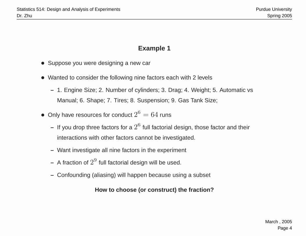
Example 1

• Suppose you were designing a new car

• Wanted to consider the following nine factors each with 2 levels

– 1. Engine Size; 2. Number of cylinders; 3. Drag; 4. Weight; 5. Automatic vs

Manual; 6. Shape; 7. Tires; 8. Suspension; 9. Gas Tank Size;

• Only have resources for conduct 26 = 64 runs

– If you drop three factors for a 26 full factorial design, those factor and their

interactions with other factors cannot be investigated.

– Want investigate all nine factors in the experiment

– A fraction of 29 full factorial design will be used.

– Confounding (aliasing) will happen because using a subset

How to choose (or construct) the fraction?

March , 2005



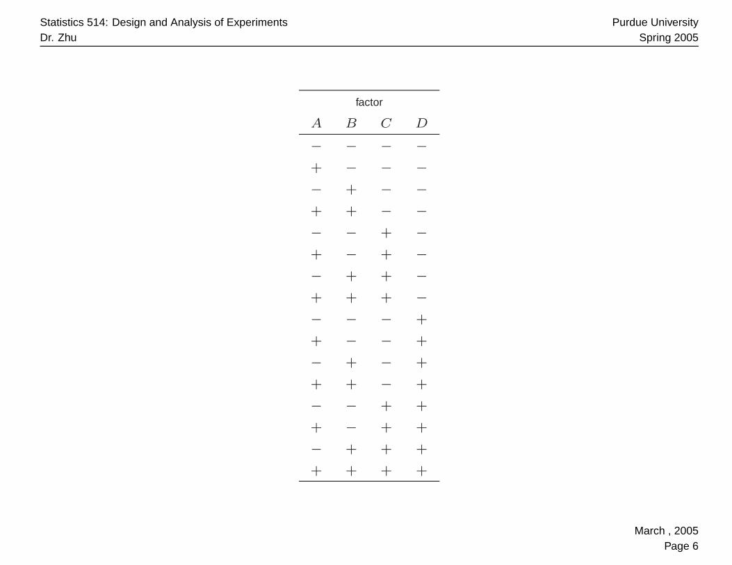
Example 2

Filtration rate experiment:

Recall that there are four factors in the experiment(A, B, C and D), each of 2 levels.

Suppose the available resource is enough for conducting 8 runs. 24 full factorial design

consists of all the 16 level combinations of the four factors. We need to choose half of

them.

The chosen half is called 24−1 fractional factorial design.

Which half we should select (construct)?

March , 2005



factor

A B C D

− − − −+ − − −− + − −+ + − −− − + −+ − + −− + + −+ + + −− − − +

+ − − +

− + − +

+ + − +

− − + +

+ − + +

− + + +

+ + + +

March , 2005



24−1 Fractional Factorial Design

• the number of factors: k = 4

• the fraction index: p = 1

• the number of runs (level combinations): N = 24

21 = 8

• Construct 24−1 designs via “confounding” (aliasing )

– select 3 factors (e.g. A, B, C) to form a 23 full factorial (basic design)

– confound (alias ) D with a high order interaction of A, B and C . For example,

D = ABC

March , 2005



factorial effects (contrasts)

I A B C AB AC BC ABC=D

1 -1 -1 -1 1 1 1 -1

1 1 -1 -1 -1 -1 1 1

1 -1 1 -1 -1 1 -1 1

1 1 1 -1 1 -1 -1 -1

1 -1 -1 1 1 -1 -1 1

1 1 -1 1 -1 1 -1 -1

1 -1 1 1 -1 -1 1 -1

1 1 1 1 1 1 1 1

• Therefore, the chosen fraction includes the following 8 level combinations:

• (−,−,−,−), (+,−,−,+), (−,+,−,+), (+,+,−,−), (−,−,+,+), (+,−,+,−),

(−,+,+,−), (+,+,+,+)

• Note: 1 corresponds to + and −1 corresponds to −.

March , 2005



Verify:

1. the chosen level combinations form a half of the 24 design.

2. the product of columns A, B, C and D equals 1, i.e.,

I = ABCD

which is called the defining relation , or ABCD is called a defining word (contrast).

March , 2005



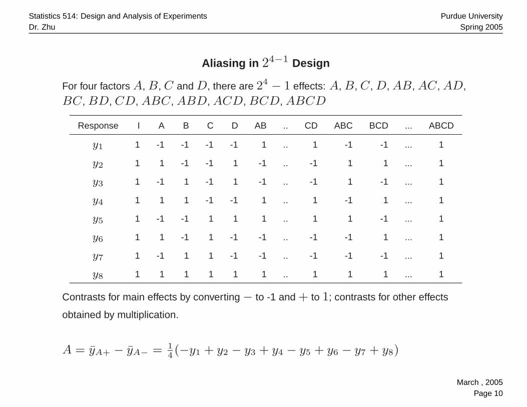
Aliasing in 24−1 Design

For four factors A, B, C and D, there are 24 − 1 effects: A, B, C , D, AB, AC , AD,

BC , BD, CD, ABC , ABD, ACD, BCD, ABCD

Response I A B C D AB .. CD ABC BCD ... ABCD

y1 1 -1 -1 -1 -1 1 .. 1 -1 -1 ... 1

y2 1 1 -1 -1 1 -1 .. -1 1 1 ... 1

y3 1 -1 1 -1 1 -1 .. -1 1 -1 ... 1

y4 1 1 1 -1 -1 1 .. 1 -1 1 ... 1

y5 1 -1 -1 1 1 1 .. 1 1 -1 ... 1

y6 1 1 -1 1 -1 -1 .. -1 -1 1 ... 1

y7 1 -1 1 1 -1 -1 .. -1 -1 -1 ... 1

y8 1 1 1 1 1 1 .. 1 1 1 ... 1

Contrasts for main effects by converting − to -1 and + to 1; contrasts for other effects

obtained by multiplication.

A = yA+ − yA− = 14(−y1 + y2 − y3 + y4 − y5 + y6 − y7 + y8)

March , 2005



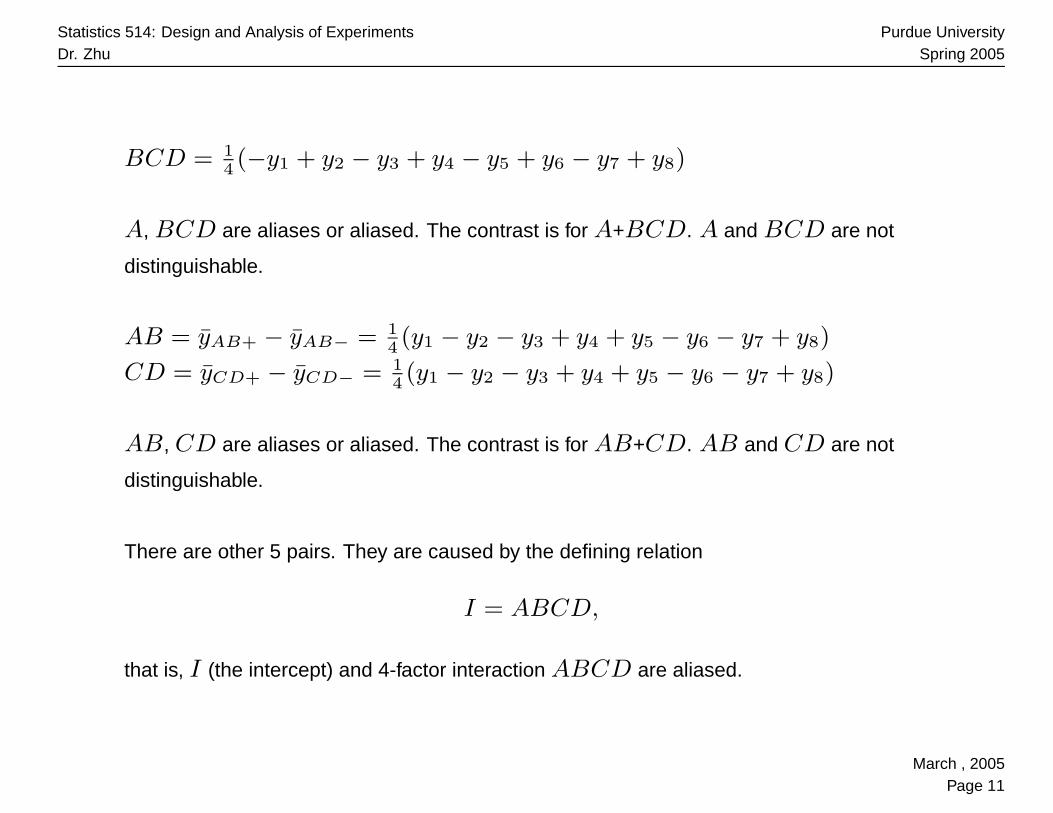
BCD = 14(−y1 + y2 − y3 + y4 − y5 + y6 − y7 + y8)

A, BCD are aliases or aliased. The contrast is for A+BCD. A and BCD are not

distinguishable.

AB = yAB+ − yAB− = 14(y1 − y2 − y3 + y4 + y5 − y6 − y7 + y8)

CD = yCD+ − yCD− = 14(y1 − y2 − y3 + y4 + y5 − y6 − y7 + y8)

AB, CD are aliases or aliased. The contrast is for AB+CD. AB and CD are not

distinguishable.

There are other 5 pairs. They are caused by the defining relation

I = ABCD,

that is, I (the intercept) and 4-factor interaction ABCD are aliased.

March , 2005



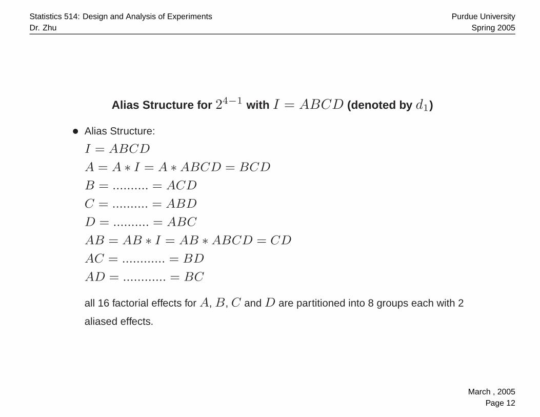
Alias Structure for 24−1 with I = ABCD (denoted by d1)

• Alias Structure:

I = ABCD

A = A ∗ I = A ∗ ABCD = BCD

B = .......... = ACD

C = .......... = ABD

D = .......... = ABC

AB = AB ∗ I = AB ∗ ABCD = CD

AC = ............ = BD

AD = ............ = BC

all 16 factorial effects for A, B, C and D are partitioned into 8 groups each with 2

aliased effects.

March , 2005



A Different 24−1 Fractional Factorial Design

• the defining relation I = ABD generates another 24−1 fractional factorial design,

denoted by d2. Its alias structure is given below.

I = ABD

A = BD

B = AD

C = ABCD

D = AB

ABC = CD

ACD = BC

BCD = AC

• Recall d1 is defined by I = ABCD. Comparing d1 and d2, which one we should

choose or which one is better?

1. Length of a defining word is defined to be the number of the involved factors.

2. Resolution of a fractioanl factorial design is defined to be the minimum length of

the defining words, usually denoted by Roman numbers, III, IV, V, etc...

March , 2005



Resolution and Maximum Resolution Criterion

• d1: I = ABCD is a resolution IV design denoted by 24−1IV .

• d2: I = ABC is a resolution III design denoted by 24−1III .

• If a design is of resolution R, then none of the i-factor interactions is aliased

with any other interaction of order less than R − i.

d1: main effects are not aliased with other main effects and 2-factor

interactions

d2: main effects are not aliased with main effects

• d1 is better, because b1 has higher resolution than d1. In fact, d1 is optimal

among all the possible fractional factorial 24−1 designs

• Maximum Resolution Criterion

fractional factorial design with maximum resolution is optimal

March , 2005



Analysis for 24−1 Design: Filtration Experiment

Recall that the filtration rate experiment was originally a 24 full factorial experiment. We

pretend that only half of the combinations were run. The chosen half is defined by

I = ABCD. So it is now a 24−1 design. We keep the original responses.

basic design

A B C D = ABC filtration rate

− − − − 45

+ − − + 100

− + − + 45

+ + − − 65

− − + + 75

+ − + − 60

− + + − 80

+ + + + 96

Let Leffect denote the estimate of effect (based on the corresponding contrast). Because of

aliasing,

March , 2005



LI → I + ABCD

LA → A + BCD

LB → B + ACD

LC → C + ABD

LD → D + ABC

LAB → AB + CD

LAC → AC + BD

LAD → AD + BC

March , 2005



SAS file for 24−1 Filtration Experiment

goption colors=(none);

data filter;

do C = -1 to 1 by 2;

do B = -1 to 1 by 2;do A = -1 to 1 by 2; D=A*B*C;

input y @@; output; end; end; end;

datalines;

45 100 45 65 75 60 80 96;

data inter; /* Define Interaction Terms */

set filter;

AB=A*B; AC=A*C; AD=A*D;

proc glm data=inter; /* GLM Proc to Obtain Effects */

class A B C D AB AC AD;

model y=A B C D AB AC AD;

estimate ’A’ A -1 1; estimate ’B’ B -1 1; estimate ’C’ C -1 1;

estimate ’D’ D -1 1; estimate ’AB’ AB -1 1; estimate ’AC’ AC -1 1;

estimate ’AD’ AD -1 1; run;

March , 2005



proc reg outest=effects data=inter; /* REG Proc to Obtain Effects */

model y=A B C D AB AC AD;

data effect2; set effects;

drop y intercept _RMSE_;

proc transpose data=effect2 out=effect3;

data effect4; set effect3; effect=col1*2;

proc sort data=effect4; by effect;

proc print data=effect4;

proc rank data=effect4 normal=blom;

var effect; ranks neff;

symbol1 v=circle;

proc gplot;

plot effect*neff=_NAME_;

run;

March , 2005



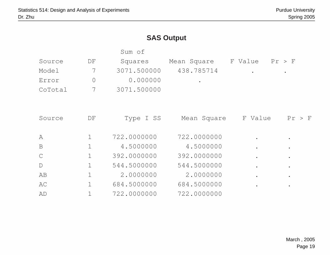
SAS Output

Sum of

Source DF Squares Mean Square F Value Pr > F

Model 7 3071.500000 438.785714 . .

Error 0 0.000000 .

CoTotal 7 3071.500000

Source DF Type I SS Mean Square F Value Pr > F

A 1 722.0000000 722.0000000 . .

B 1 4.5000000 4.5000000 . .

C 1 392.0000000 392.0000000 . .

D 1 544.5000000 544.5000000 . .

AB 1 2.0000000 2.0000000 . .

AC 1 684.5000000 684.5000000 . .

AD 1 722.0000000 722.0000000

March , 2005



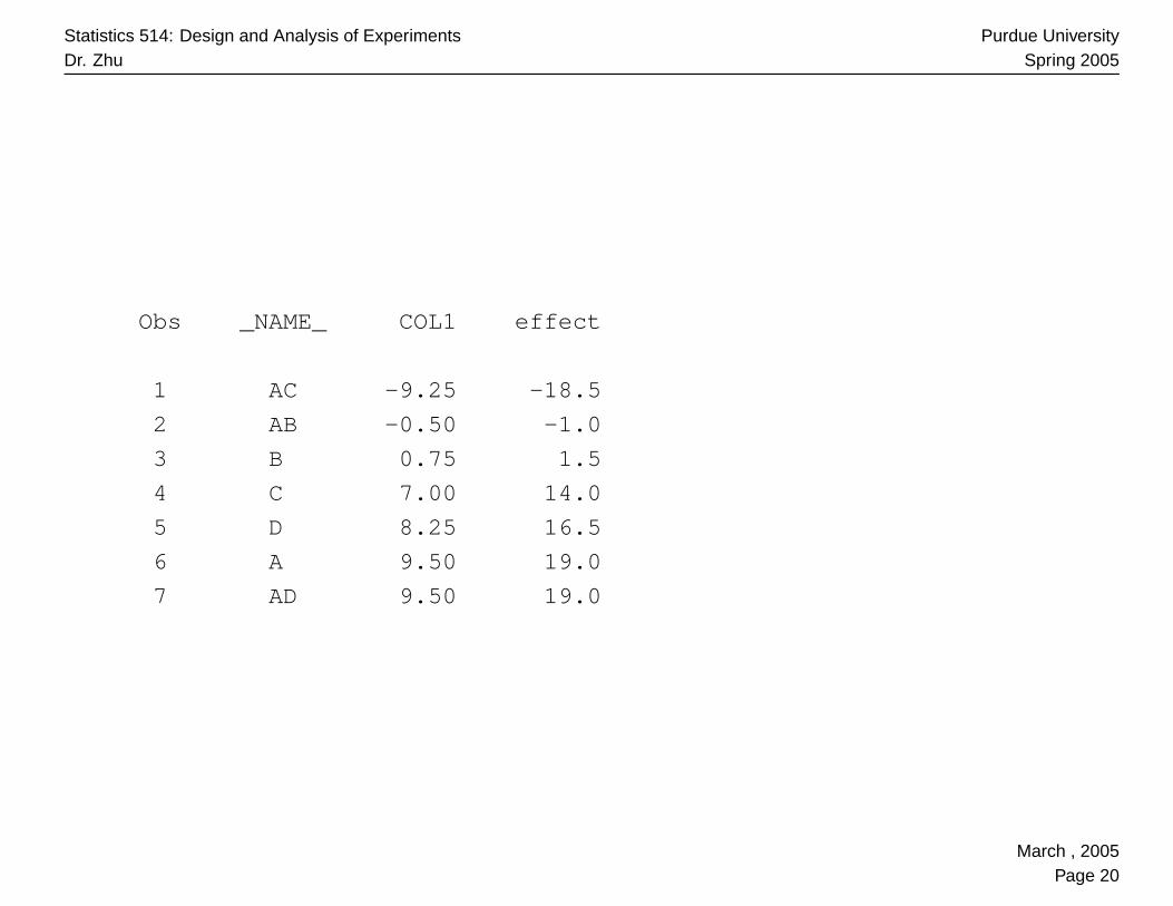
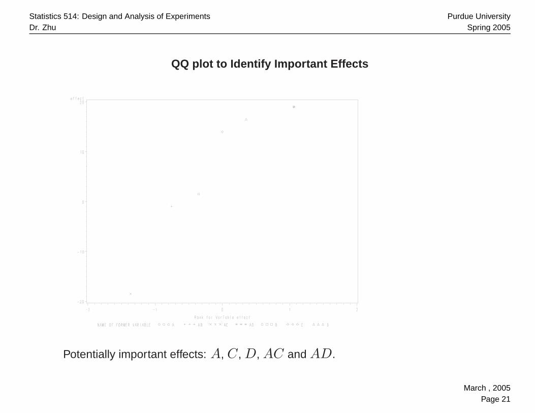
Obs _NAME_ COL1 effect

1 AC -9.25 -18.5

2 AB -0.50 -1.0

3 B 0.75 1.5

4 C 7.00 14.0

5 D 8.25 16.5

6 A 9.50 19.0

7 AD 9.50 19.0

March , 2005



QQ plot to Identify Important Effects

Potentially important effects: A, C , D, AC and AD.

March , 2005



Regression Model

Let x1, x3, x4 be the variables for factor A, C and D. The model is

y = 70.75 + 9.50x1 + 7.00x3 + 8.25x4 − 9.25x1x3 + 9.50x1x4

In Lecture 10, the regression model based on all the data (24) is

y = 70.06 + 10.81x1 + 4.94x3 + 7.31x4 − 9.06x1x3 + 8.31x1x4

It appears that the model based on 24−1 is as good as the original one.

Is this really true? The answer is NO, because the chosen effects are aliased

with other effects, so we have to resolve the ambiguities between the aliased

effects first.

March , 2005



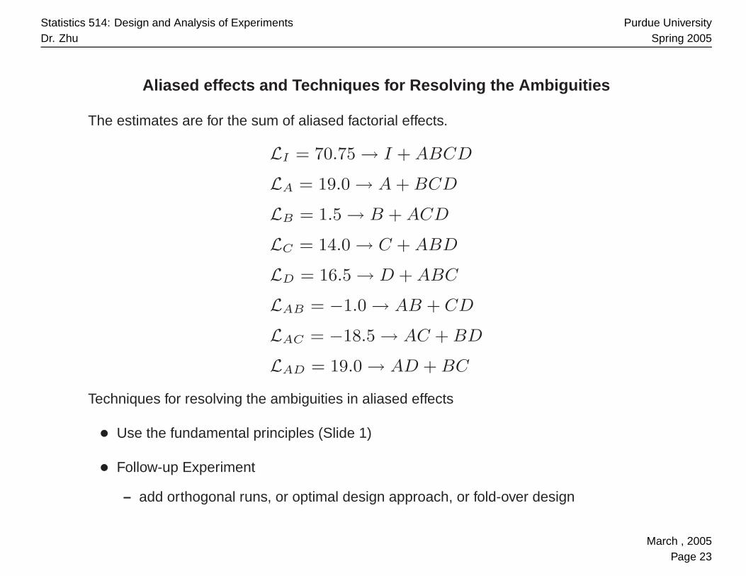
Aliased effects and Techniques for Resolving the Ambiguities

The estimates are for the sum of aliased factorial effects.

LI = 70.75 → I + ABCD

LA = 19.0 → A + BCD

LB = 1.5 → B + ACD

LC = 14.0 → C + ABD

LD = 16.5 → D + ABC

LAB = −1.0 → AB + CD

LAC = −18.5 → AC + BD

LAD = 19.0 → AD + BC

Techniques for resolving the ambiguities in aliased effects

• Use the fundamental principles (Slide 1)

• Follow-up Experiment

– add orthogonal runs, or optimal design approach, or fold-over design

March , 2005



Sequential Experiment

If it is necessary, the remaining 8 runs of the original 24 design can be conducted.

• Recall that the 8 runs we have used are defined defined by I = ABCD. The

remaining 8 runs are indeed defined by the following relationship

D = −ABC, or I = −ABCD

basic design

A B C D = −ABC filtration rate

− − − + 43

+ − − − 71

− + − − 48

+ + − + 104

− − + − 68

+ − + + 86

− + + + 70

+ + + − 65

I = −ABCD implies that: A = −BCD, B = −ACD, . . . , AB = −CD . . .

March , 2005



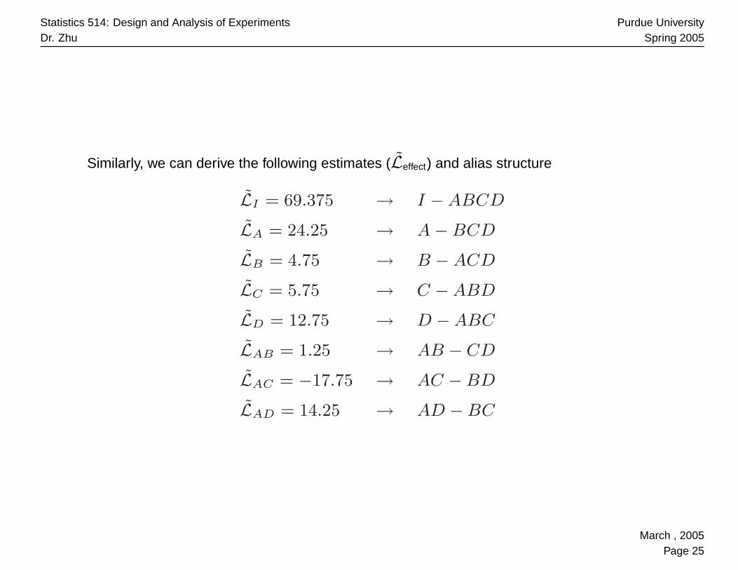
Similarly, we can derive the following estimates (Leffect) and alias structure

LI = 69.375 → I − ABCD

LA = 24.25 → A − BCD

LB = 4.75 → B − ACD

LC = 5.75 → C − ABD

LD = 12.75 → D − ABC

LAB = 1.25 → AB − CD

LAC = −17.75 → AC − BD

LAD = 14.25 → AD − BC

March , 2005



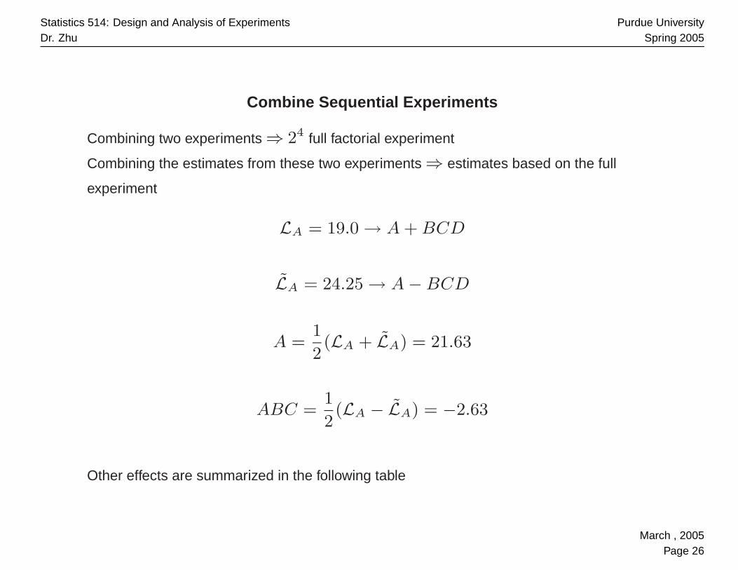
Combine Sequential Experiments

Combining two experiments ⇒ 24 full factorial experiment

Combining the estimates from these two experiments ⇒ estimates based on the full

experiment

LA = 19.0 → A + BCD

LA = 24.25 → A − BCD

A =1

2(LA + LA) = 21.63

ABC =1

2(LA − LA) = −2.63

Other effects are summarized in the following table

March , 2005



i 12(Li + Li)

12(Li − Li)

A 21.63→ A -2.63 → BCD

B 3.13→ B -1.63 → ACD

C 9.88→ C 4.13 → ABD

D 14.63→ D 1.88 → ABC

AB .13→ AB -1.13 → CD

AC -18.13→ AC -0.38 → BD

AD 16.63→ AD 2.38 → BC

We know the combined experiment is not a completely randomized experiment. Is there

any underlying factor we need consider? what is it?

March , 2005



General 2k−1 Design

• k factors: A, B, . . . , K

• can only afford to run half of all the combinations (2k−1)

• Basic design: a 2k−1 full factorial for k − 1 factors: A, B, . . . , J .

• The level of the kth factor is determined by alasing K with ABC....J , i.e.,

K = ABC · · · J• Defining relation: I = ABCD....IJK . Resolution=k

• 2k factorial effects are partitioned into 2k−1 groups each with two aliased effects.

• only one effect from each group (the representative) should be included in ANOVA or

regession model.

• Use fundamental principles, domain knowledge, follow-up experiments to de-alias.

March , 2005

fractional factorial design - purdue universityyuzhu/stat514s05/lecnot/temp0420.pdf · statistics...

Documents