Fractional Factorials

Gary W. Oehlert

School of StatisticsUniversity of Minnesota

November 12, 2014

In many situations we can identify lots of potential treatmentfactors — 10, 15 maybe 20 factors.

The smallest complete 10 factor design is the 210; it has 1,024treatments.

The smallest complete 20 factor design has 1,048,576 treatments.

These designs are simply too large to be feasible.

One good thing about factorials is that they allow us to estimateinteractions.

One bad thing about factorials is that they “spend” degrees offreedom (which correspond to resources) estimating high orderinteractions.

For example, in a 28 design (255 treatment df), 163 of the 255 dfare used estimating 4, 5, 6, 7, and 8 way interactions.

This is good if the interactions are important, but wasteful if wethink high order interactions are small relative to main effects andlow order interactions.

Elephant and the Flea Principle

When you want to weigh the elephant, don’t worry about his fleas.

If you think main effects and low order interactions are big andhigh order interactions are small, then don’t sweat the high orderinteractions.

(Of course, if high order interactions aren’t small, you could have aproblem.)

Fractioning

As an alternative to a full factorial, suppose that we keep all of thefactors but only run part of the factorial design, a fraction of thefactorial.

How do we choose the fraction?

How do we analyze the results?

We have less data, what did we lose going to a fraction?

Did we gain anything going to a fraction?

Fractional factorials are smaller designs that let us look at maineffects and (potentially) low order interactions.

This makes sense in situations such as:

1 We believe many of the factors are inert and we are simplyscreening to find the factors that are not inert.

2 We believe that any high order interactions are small enoughto ignore (elephant and flea principle).

3 We must shrink the design and are willing to take certain risks(discussed below) to do so.

Fractioning the two-series

We will discuss “regular” fractions of the two-series design. Thereare non-regular fractions, and you can fraction other designsbesides the two-series.

We will build half fractions, quarter fractions, eighth fractions, andso on.

The shorthand is 2k−1 for a half fraction of a 2k , 2k−2 for aquarter fraction, and so on. In general, 2k−p.

A flip suggestion for generating a 2k−p design would be toconfound a 2k into 2p blocks, but only run one of the blocks.

In fact, that is exactly equivalent to what we do.

In practice we don’t do it that way because there is an easier wayto generate the same design.

Choose p defining contrasts. These will be generators for ourdesign.

For one defining contrast W, we will use either the block withW=1 or the block with W= –1.

By convention, I is a column of all ones. Thus we will either haveI=W or I=–W.

Consider a 23−1 with I=ABC. This is the fraction where the ABCinteraction is always 1.

A B C AB . . . ABC

a 1 –1 –1 –1 1b –1 1 –1 –1 1c –1 –1 1 1 1

abc 1 1 1 1 1

Note that the C contrast matches the AB contrast, and ABC isalways 1. There are also always an odd number of A, B, and C atthe high level in this particular design.

Try this again with I=–ABC. This is the fraction where the ABCinteraction is always –1.

A B C AB . . . ABC

(1) –1 –1 –1 1 –1ab 1 1 –1 1 –1ac 1 –1 1 –1 –1bc –1 1 1 –1 –1

Note that the C contrast is always the negative the AB contrast,and ABC is always –1. There are also always an even number of A,B, and C at the high level.

Note: you cannot count on even begin –1 and odd being 1. Thosewill change depending on the number of factors in the model andthe number of factors in the defining contrast.

To get a quarter fraction, we need two defining contrasts W1 andW2. Our fraction will either be the –1/–1, –1/1, 1/–1, or 1/1combinations.

Let’s look at a 25−2 generated by I=ACE and I=–BCD.

A B C D E AC BC . . . ACE BCD ABDE

e –1 –1 –1 –1 1 1 1 1 –1 –1a 1 –1 –1 –1 –1 –1 1 1 –1 –1

bde –1 1 –1 1 1 1 –1 1 –1 –1abd 1 1 –1 1 –1 –1 –1 1 –1 –1cd –1 –1 1 1 –1 –1 –1 1 –1 –1

acde 1 –1 1 1 1 1 –1 1 –1 –1bc –1 1 1 –1 –1 –1 1 1 –1 –1

abce 1 1 1 –1 1 1 1 1 –1 –1

Note that ACE is always 1 and BCD is always –1; also, ABDE isalways –1. Note further that the D contrast is always the reverseof the BC contrast, and the E contrast is the same as the ACcontrast.

Aliasing

The D contrast is the reverse of the BC contrast, so D cannot bedistinguished from –BC; they are aliases of each other.

The E contrast is the same as the AC contrast, so E cannot bedistinguished from AC; they are aliases of each other.

In a half fraction, each factorial contrast will come with two names(aliases). In a quarter fraction, each factorial contrast will comewith four names (aliases).

We did not get something for nothing!

The price we pay for fractioning is that every factorial degree offreedom comes with multiple aliases. Within the context of the

experiment, we cannot distinguish between the aliases.

However, if potentially large main effects (the elephants) arealways aliased with assumed to be small interactions (the fleas),then we are essentially looking at the main effects (when weighingan elephant with its fleas, you’re really getting a weight of theelephant).

Let’s repeat.

We have I=–BCD, and we also have D=–BC.

We have I=ACE, and we also have E=AC.

We have I=–ABDE, and we also have AB=–DE (not shownabove).

Finding aliases

In a quarter fraction, we have I=W1 and I=W2, so we also haveI=W1W2.

In our example: I=ACE and I=–BCD, so we also have I=–ABDE(reduce exponents mod 2).

Again, we have I = W1 = W2 = W1W2, so we also haveA = AI = AW1 = AW2 = AW1W2

I = ACE = –BCD = –ABDE, soA = CE = –ABCD = –BDE (reduce exponents mod 2).

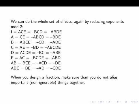
We can do the whole set of effects, again by reducing exponentsmod 2:I = ACE = –BCD = –ABDEA = CE = –ABCD = –BDEB = ABCE = –CD = –ADEC = AE = –BD = –ABCDED = ACDE = –BC = –ABEE = AC = –BCDE = –ABDAB = BCE = –ACD = –DEABC = BE = –AD = –CDE

When you design a fraction, make sure than you do not aliasimportant (non-ignorable) things together.

Generating fractions made easy

Now there is a welcome topic!

In a 2k−p design, there is some set of k-p factors for which thefraction is a complete design (when you ignore the other p factors).

In fact, there are usually lots of sets of k-p factors that will work.You just need a set where none of the effects or interactions ofthose factors is aliased to I.

In our I = ACE = –BCD = –ABDE example, any set of threeexcept ACE and BCD will work.

I call this included factorial the base factorial.

It will be the case that any other factor will be aliased to someinteraction of the factors in the base factorial.

In our I = ACE = –BCD = –ABDE example, A, B, and C canform a base factorial. Then D=–BC and E=AC.

Or we could have used A, D, and E for our base factorial. ThenB=–ADE and C=AE.

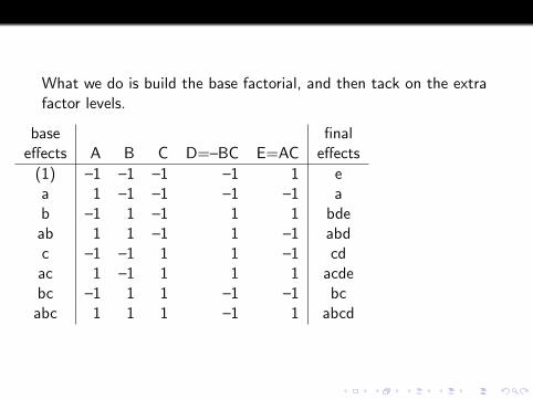
What we do is build the base factorial, and then tack on the extrafactor levels.

base finaleffects A B C D=–BC E=AC effects

(1) –1 –1 –1 –1 1 ea 1 –1 –1 –1 –1 ab –1 1 –1 1 1 bde

ab 1 1 –1 1 –1 abdc –1 –1 1 1 –1 cd

ac 1 –1 1 1 1 acdebc –1 1 1 –1 –1 bc

abc 1 1 1 –1 1 abcd

Analysis

Analyze a 2k−p as a complete factorial in the base factors.

But don’t forget the aliasing!

Suppose you analyze our example using factors A, B, and C, andthe BC interaction alone looks big.

Remember that BC=ABE=–D=–ACDE. What you are seeing isprobably, but not for certain, the D main effect.

Portents of things to come. We are still in our example withI = ACE = –BCD = –ABDE

Suppose thatA = CE = –ABCD = –BDEC = AE = –BD = –ABCDEE = AC = –BCDE = –ABDlook big.

Is that three main effects, or is it A, C, and AC (or A, E and AE)(or C, E, and CE)?

You cannot distinguish these four situations from within the data.There is a potential price for using a fraction!

Resolution and aberration

In a resolution R design, no j-factor effect is aliased to anythingwith fewer than R-j factors.

In our regular designs, resolution is just the minimum number ofletters in an alias of I.

Resolution is usually denoted by a Roman numeral.

Our I = ACE = –BCD = –ABDE example is a 25−2III design.

Higher resolution is better.

Resolution III designs don’t alias main effects, but they do aliasmain effects and two factor interactions. Resolutions III designs aresometimes called “main effects” designs.

Resolution IV designs don’t alias main effects to two factorinteractions, but they do alias two factor interactions to other twofactor interactions.

Resolution V designs do not alias any main effects or two factorinteractions to each other.

Not only do we want the resolution to be as high as possible, wewant as few as possible of those short aliases.

Aberration is really just a count of the number of alias of I ofdifferent lengths (3, 4, 5, etc letters).

Design A has smaller aberration than design B if the A has asmaller number in the first digit where they differ.

Lower aberration is better.

Three different 27−2IV plans. Each design has lower aberration than

the ones above it.

AberrationDesign 3 4 5 6 7

I=ABCF=BCDG=ADFG 0 3 0 0 0I=ABCF=ADEG=BCDEFG 0 2 0 1 0I=ABCDEF=ABCEG=DEFG 0 1 2 0 0

Projection

Any resolution R design contains a complete factorial in any R-1factors.

This factorial could be replicated.

There could be sets of R or more factors that also form a completefactorial, but no guarantees.

If you think that there shouldn’t be more than 3 active factors(with the rest inert), then a resolution IV design would allow youto get all their main effects and interactions, and you don’t evenneed to know which three.

The trick is the assumption that there can’t be more than three.

One possible approach to analyzing a fraction is to do the Danielplot to identify a few active factors, then project down onto thosefactors.

Projecting down means just looking at those factors (and theirinteractions), using other df for error.

This is common practice, but still somewhat suspect in that youhave made the big factors “treatments” and the little factors“error”. The p-values are not unassailable.

Blocking (confounding)

We know how to block a two-series into 2, 4, 8, etc blocks.

We do exactly the same thing in a fraction, but each confoundedeffect has multiple aliases.

Be sure not to confound something important.

Our example has I = ACE = –BCD = –ABDE, and one of thealias sets is AB = BCE = –ACD = –DE.

To get two blocks of four, put the four runs with an even numberof a’s and b’s in one block and the odds in the other.

The treatments are e, a, bde, abd, cd, acde, bc, and abcd. Thetwo blocks are thus (e, abd, cd, abcd) and (a, bde, acde, bc).

Realistically, doing this would try to get too much out of 8 runs (5main effects and a block).

Dealiasing

We have seen that aliasing can sometimes leave us in a situationwhere there is more than one reasonable explanation of the “large”effects.

There is no way to resolve this ambiguity internal to the data; wecan only resolve this with more information.

More information usually means collecting more data, but it could,in principle, mean using outside information (the literature, otherexperiments, etc) to resolve the question.

We will discuss the simplest form(s) of collecting more data toremove troublesome aliasing.1

The practice of “breaking” the bad aliasing is called dealiasing.

Our version of dealiasing is based on running additional fractions ofthe factorial.

For example, we might go from a one-eighth replication to aone-quarter replication. The question is, which additional eightfraction should we run?

1Sounds like removing those troublesome stains from your laundry.

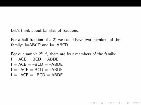
Let’s think about families of fractions.

For a half fraction of a 24 we could have two members of thefamily: I=ABCD and I=–ABCD.

For our sample 25−2, there are four members of the family:I = ACE = BCD = ABDEI = ACE = –BCD = –ABDEI = –ACE = BCD = –ABDEI = –ACE = –BCD = ABDE

A different set of generators give us a different family of fractions.

For example, here is a different 25−2 with a different family:I = ABD = CDE = ABCEI = ABD = –CDE = –ABCEI = –ABD = CDE = –ABCEI = –ABD = –CDE = ABCE

When we have a fraction, we will dealias by choosing anotherfraction from the same family.

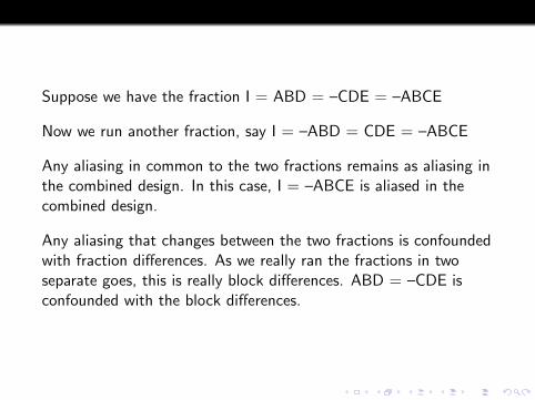
Suppose we have the fraction I = ABD = –CDE = –ABCE

Now we run another fraction, say I = –ABD = CDE = –ABCE

Any aliasing in common to the two fractions remains as aliasing inthe combined design. In this case, I = –ABCE is aliased in thecombined design.

Any aliasing that changes between the two fractions is confoundedwith fraction differences. As we really ran the fractions in twoseparate goes, this is really block differences. ABD = –CDE isconfounded with the block differences.

Example. We run a 27−4 design with generators ABCD, BCE,ACF, and ABG.

The aliases of I are I = ABCD = BCE = ACF = ABG = ADE =BDF = ABEF = CDEF = CDG = ACEG = BDEG = BCFG =ADFG = EFG = ABCDEFG.

If the contrasts corresponding to A, D, and F are big, we are OK,it’s probably the main effects. No dealiasing is needed.

But if the contrasts corresponding to A, D, and E are big, then wehave ambiguity, and we can fix it by dealiasing.

Any other member of the family of fractions that has I = –ADEwill break that aliasing. For example,

I = ABCD = –BCE = –ACF = –ABG = –ADE = –BDF = ABEF= CDEF = –CDG = ACEG = BDEG = BCFG = ADFG = –EFG= –ABCDEFG.

Aliasing in common: I = ABCD = ABEF = CDEF = ACEG =BDEG = BCFG = ADFG

Aliasing that changed: –BCE = –ACF = –ABG = –ADE = –BDF= –CDG = –EFG = –ABCDEFG.

We began with resolution III and ended with resolution IV.

Resolution IV is the best you can do with a 27−3, so we were notmuch worse off doing two sixteenths than if we had done an eighthto begin with.

In some cases, you could get more resolution if you had designedthe larger experiment from the start, but you miss the chance offinding all you need with a smaller design.

Sequences of small fractions can sometimes be better than onelarger fraction.

Example. 7 factors, at most 32 runs. Assume that at most 4factors are active, and assume that all three way interactions arenegligible.

The best you can do with a 32 run design is 27−2IV . For example,

I = ADEF = ABCDG = BCEFG.

Resolution IV is not really good enough if ADEF happen to beyour active factors, because you will still alias some potentiallyactive two factor interactions together.

However, try starting with a 27−3IV . For example, I = BCDE =

ACDF = ABCG = ABEF = ADEG = BDFG = CEFG.

This design is good enough for any set of four active factors exceptthe seven sets of four that form aliases of I. Most of the time, wecan get what we need with 16 units.

If our big effects are from one of those sets of four, say B, C, D,and E, then run another 16 runs that change the sign of BCDE.For example, I = –BCDE = ACDF = ABCG = –ABEF = –ADEG= BDFG = –CEFG.

Combined with the first fraction this breaks the BCDE aliasing.

Take away points.

Running 32 runs at once could not get the resolution weneeded, although it is good enough for nearly all sets of fouractive factors.

Often, 16 runs is good enough for sets of four active factors.

Running 16 runs, taking a look, and then running another 16runs does not get resolution V, but it can break all importantaliasing.

The trick is the first 16 runs scout out the ground so that wecan choose the second 16 runs optimally.

This sort of thing works best when signal is large relative to noise.

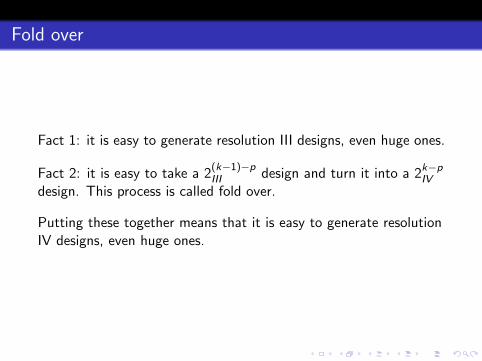
Fold over

Fact 1: it is easy to generate resolution III designs, even huge ones.

Fact 2: it is easy to take a 2(k−1)−pIII design and turn it into a 2k−p

IVdesign. This process is called fold over.

Putting these together means that it is easy to generate resolutionIV designs, even huge ones.

Construct a 2k−pIII design. We can do this as long as 2k−p > k .

Simply begin with a base factorial in k-p factors, then alias theremaining p factors to any interactions of the base factors.

This will be a resolution III design.

Fold over.

1. Write out your 2(k−1)−pIII design using +/– notation.

2. Make another set of 2(k−1)−p by reversing all the signs in the

first 2(k−1)−pIII design.

3. Add the kth factor by making it – for the first 2(k−1)−p runsand + for the last 2(k−1)−p runs.

This process breaks all the odd length aliases, typically leaving uswith resolution IV.

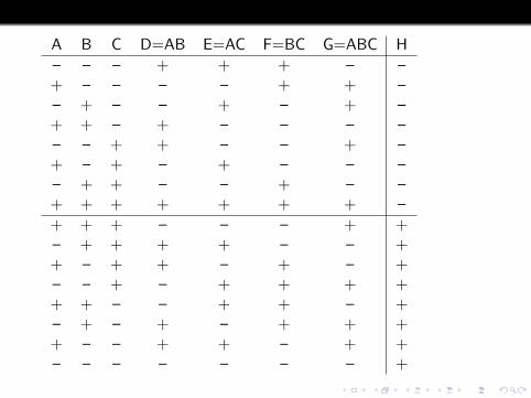
A B C D=AB E=AC F=BC G=ABC H

– – – + + + – –+ – – – – + + –– + – – + – + –+ + – + – – – –– – + + – – + –+ – + – + – – –– + + – – + – –+ + + + + + + –

+ + + – – – + +– + + + + – – ++ – + + – + – +– – + – + + + ++ + – – + + – +– + – + – + + ++ – – + + – + +– – – – – – – +

What happened to the generators?

D=AB becomes D=–ABHE=AC becomes E=–ACHF=BC becomes F=–BCHG=ABC remains G=ABC

That one wasn’t so bad, and it could be in a table.

What if you want a 221−15IV ; you’re not going to find that one in the

back of the book.

Start with a 220−15III , then fold over.