fractures and discontinuities

2.1 Introduction

From the hydrogeological point of view, fractures and discontinuities are amongst the most important of geo-logical structures. Most rocks possess fractures and other discontinuities (Fig. 2.1) which facilitate storage and movement of fluids through them. On the other hand, some discontinuities, e.g. faults and dykes may also act as barriers to water flow. Porosity, permeabil-ity and groundwater flow characteristics of fractured rocks, particularly their quantitative aspects, are rather poorly understood. Main flow paths in fractured rocks are along joints, fractures, shear zones, faults and other discontinuities.

There is a great need to understand hydraulic char-acteristics of such rocks, in view of: (a) groundwater development, to meet local needs; and (b) as deposito-ries for nuclear and other toxic wastes.

There could be multiple discontinuities in fractured rocks along which groundwater flow takes place. A number of factors including stress, temperature, rough-ness, fracture geometry and intersection etc. control the groundwater flow through fractures. For example, fracture aperture and flow rate are directly interrelated; non-parallelism of walls and wall roughness lead to friction losses; hydraulic conductivity through frac-tures is inversely related to normal stresses and depth, as normal stress tends to close the fractures and reduce the hydraulic conductivity.

It has also been noted that fracture permeability reduces with increasing temperature. As temperature increases with depth, thermal expansion in rocks takes place which leads to reduction in fracture aperture and corresponding decrease in permeability. Further the permeability is also affected by cementation, filling, age and weathering (see Chap. 8).

Parallel fractures impart a strong anisotropy to the rock mass. On the other hand, greater number of more interconnected fractures tends to reduce anisotropy. Further, larger fracture lengths, greater fracture density and larger aperture increase hydraulic conductivity.

Therefore, summarily, for hydrogeological studies, it is extremely important to understand and describe the structure of the rock-mass and quantify the pattern and nature of its discontinuities (van Golf-Racht 1982; Sharp 1993; Lee and Farmer 1993; de Marsily 1986).

2.2 Discontinuities—Types, Genetic Relations and Significance

Discontinuity is a collective term used here to include joints, fractures, bedding planes, rock cleavage, folia-tion, shear zones, faults and other contacts etc. In this discussion using a genetic approach, we group discon-tinuities into the following categories:

1. Bedding plane2. Foliation including cleavage3. Fractures (joints)4. Faults and shear zones, and5. Other geological discontinuities.

2.2.1 Bedding Plane

Primary bedding and compositional layers in sedimen-tary rocks form the bedding plane. Usually, it is the most significant discontinuity surface in all sedimen-tary rocks such as sandstones, (Fig. 2.1b) siltstones, shales etc., except in some massive sandstones or

2Fractures and Discontinuities

B. B. S. Singhal, R. P. Gupta, Applied Hydrogeology of Fractured Rocks, DOI 10.1007/978-90-481-8799-7_2, © Springer Science+Business Media B.V. 2010

��

�� Fractures and Discontinuities

limestones. Bedding plane can be readily identified in the field owing to mineralogical-compositional-tex-tural layering.

Bedding plane, being the most important disconti-nuity, imparts anisotropy and has a profound influence on groundwater flow in the vadose zone. The ground-water flow is by-and-large down-dip (Fig. 2.2).

Folds are flexures in rocks formed due to warping of rocks. Although a wide variety of folds are dis-tinguished, the two basic types are anticlines (limbs dipping away from each other) and synclines (limbs dipping towards each other). Folding leads to change or reversal in dip directions of beds, and this affects groundwater flow. Further, folding is accompanied by fracturing of rocks. In an anticline, the crest undergoes higher tensional stresses and hence develops open

tensile fractures, which may constitute better sites for groundwater development.

2.2.2 Foliation

Foliation is the property of rocks, whereby they break along approximately parallel surfaces. The term is restricted to the planes of secondary origin occurring in metamorphic rocks. Foliation develops due to par-allel-planar alignment of platy mineral grains at right angles to the direction of stress, which imparts fissil-ity. The parallel alignment takes place as a result of recrystallisation during regional dynamothermal meta-morphism, a widespread and common phenomenon

Fig. 2.1 Examples of frac-tured rocks; a Metamorphic rocks (meta-argillites) in Khe-tri Copper Belt, India. Several sets of fractures including shear planes are developed; some of the fractures pos-sess infillings. b Sandstones of Vindhyan Group, India; bedding planes constitute the dominant discontinuity surfaces. (Photograph (b) courtesy of A.K. Jindal)

Fig. 2.2 Schematic diagram showing the role of bedding planes and fractures on groundwater movement in the vadose zone

GROUNDWATER FLOWBEDDING/FOLIATIONFRACTURESWATER TABLE

REGIONAL GROUNDWATER FLOW

A B

�.� Discontinuities—Types, Genetic Relations and Significance ��

in crystalline rocks. Rock cleavage is almost a syn-onymous term. It is also used for planes of secondary origin along which the rock has a tendency to break in near-parallel surfaces. Some terms are used for spe-cific metamorphic rocks. Thus, the term slaty cleav-age is used for rock cleavage in slates; schistosity is used for schists and gneissosity for gneisses. Foliation planes may or may not be parallel to bedding. Folia-tion that is parallel to the bedding is often referred to as bedding foliation. Fracture cleavage is produced by closely-spaced jointing. In many schistose rocks, shear cleavages are developed due to closely spaced shear-slip planes, known as slip-cleavage. In a folded region, the foliation often developed parallel to the axial plane of folds is called the axial plane foliation.

Foliation in metamorphic rocks has a profound influence on groundwater movement, possessing quite the same role as bedding in the sedimentary rocks, both being the most significant discontinuities in the respective rock categories (e.g. see Fig. 2.2).

2.2.3 Fractures and Joints

2.2.3.1 Introduction and Terminology

Fractures, also called joints, are the planes along which stress has caused partial loss of cohesion in the rock. It is a relatively smooth planar surface representing a plane of weakness (discontinuity) in the rock. Conven-tionally, a fracture or joint is defined as a plane where there is hardly any visible movement parallel to the surface of the fracture; otherwise, it is classified as a fault. In practice, however, a precise distinction may be difficult, as at times within one set of fractures, some planes may show a little displacement whereas others may not exhibit any movement. Slight move-ment at right angles to the fracture surface will pro-duce an open fracture, which may remain unfilled or may get subsequently filled by secondary minerals or rock fragments.

‘Fracture zones’ are zones of closely-spaced and highly interconnected discrete fractures. They may be quite extensive (length > several kilometres) and may even vary laterally in hydraulic properties.

Fracture-discontinuities are classified and described in several ways using a variety of nomenclature, such as: joints, fracture, fault, shear, gash, fissure, vein etc.

Generally, the term fracture is used synonymously with joint, implying a planar crack or break in rock without any displacement. The terms fault and shears are used for failure planes exhibiting displacement, parallel to the fracture surfaces. Gash is a small-scale open ten-sion fracture that occurs at an angle to a fault. Fissure is a more extensive open tensile fracture. A filled- fissure is called a vein.

An individual fracture has a limited spatial extent and is discontinuous in its own plane (Fig. 2.3). On any outcrop, fractures have a certain trace lengths and fracture spacings. By mutual intersection, the various fracture sets may form interconnected continuous net-work, provided that the lengths of the joints in the dif-ferent sets are much greater than the spacings between them (see Fig. 2.18). The interconnectivity of fractures leads to greater hydraulic conductivity.

2.2.3.2 Causes of Fracturing

Although fractures are extremely common and wide-spread in rocks, geologically they are still not well-enough studied (Price and Cosgrove 1990). Complex processes are believed to be involved in the origin of fractures, which are related to geological history of the area. Fractures are created by stresses which may have diverse origin, such as: (a) tectonic stresses related to the deformation of rocks; (b) residual stresses due to events that happened long before the fracturing; (c) contraction due to shrinkage because of cooling of magma or dessication of sediments; (d) surficial

Fig. 2.3 Two sets of fractures are schematically shown in the block. An individual fracture has limited spatial extent and is discontinuous in its own plane. Fracture spacing and fracture trace length are indicated for one set

Fracturespacing

Length of fracture trace


movements such as landslides or movement of gla-ciers; (e) erosional unloading of deep-seated rocks; and (f) weathering, in which dilation may lead to irregular extension cracks and dissolution may cause widening of cavities, cracks etc.

2.2.3.3 Types of Fractures

Firstly, fractures may be identified into two broad types: (a) systematic, which are planar, and more regular in distribution; and (b) non-systematic, which are irregu-lar and curved (Fig. 2.4). The non-systematic fractures meet but do not cross other fractures and joints, are curved in plan and terminate at bedding surface. They are minor features of dilational type and develop in the weathering zone. Curvilinear pattern is their general characteristic. Parallel systematic fractures are treated as a set of fractures.

Geometric classification—Considering the geo-metric relationship with bedding/foliation, the system-atic fractures or joints are classified into several types. Strike joints are those that strike parallel to the strike of the bedding/foliation of the rock. In dip joints, the strike direction of joints runs parallel to the dip direc-tion of the rock. Oblique or diagonal joints strike at an angle to the strike of the rocks. Bedding joints are essentially parallel to the bedding plane of the associ-ated sedimentary rock.

Depending upon their extent of development, frac-tures may be classified into two types: first-order and second-order. First-order fractures cut through several layers of rocks; second-order fractures are limited to a single rock layer. Further, depending upon the strike trend of fractures with respect to the regional fold axis, fractures are designated as longitudinal (paral-

lel), transverse (perpendicular) or oblique ones (see Fig. 2.7 later).

Genetic classification—Genetically, the systematic fractures can be classified into three types:

1. Shear fractures, which may (or may not) exhibit shear displacement and are co-genetically developed in conjugate sets with a dihedral angle 2i > 45°.

2. Dilational fractures, which are of tensile origin, commonly, developed perpendicular to the bedding plane, and are open fractures with no evidence of shear movement.

3. Hybrid fractures, which exhibit features of both shear and dilational origin. They may occur in con-jugate sets with a dihedral angle 2i < 45°. They are open (extension!), may be partly filled with veins, and may also exhibit some shear displacement.

The physical stress conditions under which these three types of fractures develop are illustrated by the Mohr diagram in Fig. 2.5. The curve ABC is a Mohr enve-lope. The stress circles touching the Mohr envelope at A, B and C points indicate different failure condi-tions of the rock. In condition ‘A’, the principal maxi-mum compressive stress is negative, i.e. extensional, and therefore it leads to a dilational failure. In condi-tion, ‘C’, a typical conjugate shear failure takes place, such that the dihedral angle 2i > 45°. ‘B’ represents a condition that there is a positive maximum principal compressive stress and a negative minimum princi-pal compressive stress, i.e. the effective normal stress perpendicular to the fracture plane is negative (exten-sional). This can be attributed to high fluid pressure conditions at depth. Hence, there is a tendency for such shear fractures to open and also get filled with miner-als. Typically, in such hybrid shear-extension fractures, the dihedral angle is 2i < 45°.

Conjugate shear fractures developing at greater depths are of ductile nature and possess a large 2i (~90°). On the other hand, conjugate brittle shears develop at a shallower depth and possess a smaller 2i (~60°). Further, brittle deformation causes derivative shears of several orders to form successively deviating trends, which cause a spread in the trends of conju-gate shears (Ruhland 1973). The process of shearing is also accompanied by tensile deformation. Thus, brittle deformation may produce fractures of different magni-tude and direction in successive orders. In a rock mass fractured by three orders of brittle deformation, tensile

Fig. 2.4 Systematic and non-systematic types of fractures

a : Systematic fracturesb : Non-systematic fractures

a ba

b


fracturing may spread over a range of about 75° and shear fracturing over a range of nearly 135° (Fig. 2.6).

2.2.3.4 Discrimination Between Shear and Extension Fractures

The rheological principles indicate that there is no sharp categorization between extension and shear frac-tures. In fact, all gradations from one category to the other take place. However, from hydrogeological point of view, it is important to distinguish between shear and extension joints as dilational joints are more open and possess greater hydraulic conductivity than shear joints. Discrimination between shear and tension joints may be difficult, particularly in complexly deformed areas. However, the following features may help in their discrimination:

1. Shear joints may exhibit displacement parallel to the plane of the joints, which is absent in the case of extension joints.

2. Shear joints commonly occur in conjugate sets which may be indicated by a statistical analysis.

3. In field, slickensides and other criteria of relative movement may be observed in the case of shear joints.

4. Generally, extension joints are open and shear joints are tight.

5. The orientation of the joints with respect to the bed-ding/foliation and or fold-axis can provide infor-mation on shear vs. tensile origin of fractures, as shear joints occur in oblique conjugate sets whereas extension joints occur as longitudinal and trans-verse joints forming an orthogonal pair (Fig. 2.7).

6. The cumulative trend diagram of fractures may also provide information on the related stress field,

Fig. 2.5 Basic genetic types of fractures: A extension frac-ture; B hybrid extension-shear fracture; C shear fracture. The Mohr diagram indicates the stress conditions for these failures. σ1 and σ3 are the maximum and minimum principal compressive stresses respectively

Mohr envelope

C

Mohr circle

C

Normal stress

A

B

She

arin

g st

ress

Extensionfailure

Hybrid extension-shearfailure

2θ <45° 2θ′>45°

Shearfailure

σ3

σ3

σ1

σ3

σ1 σ1

σ1σ3 θ′θ

A B


and therefore the likely trends of shear and exten-sion fractures; the maximum principal compressive stress bisects the dihedral angle of conjugate shear fractures and is parallel to the tensile fracture.

A field example of large-scale tensional and shear fractures extending for several kilometres is given in Fig. 2.8 where tensional fractures appear as wide open and shear joints are characterized by relative displacements.

2.2.3.5 Orientation of Fractures vis-à-vis Regional Structure

Ideally, in the case of simple-dipping strata, four sets of fractures (systematic) develop (Fig. 2.7). S1 and S2 form a conjugate set of shear fractures and T1 and T2 are extension fractures. All these fractures are perpen-dicular to the bedding plane and contain the intermedi-ate principal compressive stress σ2.

Figure 2.9 shows a simplified ideal relationship between fractures and folds. σ1 is the maximum prin-cipal compressive stress perpendicular to the fold-axis (b). A conjugate set of oblique trending right-lateral and left-lateral shear fractures develops. There are two sets of extension fractures, one longitudinal and the other transverse to the fold-axis, both being mutually orthogonal.

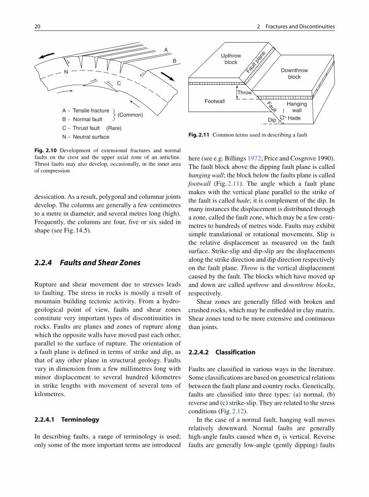
During folding, bending of a bed causes extension on the convex side and compression on the concave side (Fig. 2.10). This results in extension fractures and normal faults on the crests of anticlines. Less com-monly, thrust faults also develop in the inner areas of compression.

Fig. 2.6 Scheme of brittle deformation of a homogeneous rock mass. The rose diagram illustrates the ranges of orientations of tensile and shear fractures due to three orders of deformation. (After Ruhland 1973)

Spread of tensile deformation

Spread of shear deformation

Rose diagram

75°

135°

b

a

60°

15°

Shearfracture

Tensilefracture

Order ofdeformation

Plan view

Greatestprincipalstress

III

II

I

σ1

σ1

Fig. 2.7 Development of four sets of fractures in the case of simple dipping strata (see also Fig. 2.9)

S0

s0

: Bedding plane

T1,T

2 : Dilational fractures

S1,S

2 : Shear fractures

S1

T1

T2

S2

N


2.2.3.6 Other Types of Fractures

Sheeting joints: These joints are generally flat, some-what curved and nearly parallel to the topographic surface, often developed in granitoid rocks. They are closely developed near to the surface, and their spacing

increases with depth. They are generated due to release of overburden stress.

Columnar joints: Joints of this type are tension frac-tures generated due to shrinkage in rocks. Shrinkage may occur due to cooling or dessication. Igneous rocks contract on cooling. Mud and silt shrink because of

Fig. 2.8 a Example of large-scale tensional and shear fractures extending for several kilometres in a part of the Precambrian Cuddapah basin, India; black-and-white image generated from GoogleEarth. b Interpretation map of the above image; fractures

marked T are wide open tensional fractures that are vegetated implying groundwater seepage, S are shear fractures exhibiting lateral relative displacement at places

0.5 km0

Lithologicboundary

T

S

S

T

a b

Fig. 2.9 Ideal relationship between major joint sets in a folded bed. There are two sets of conjugate shear fractures and two sets of mutually orthogonal dilational fractures. All the fractures are shown vertical

Fold axis (b)

Transversefracture

Orthogonal fractures

Right lateral

Longitudinalfracture

Left lateral

60°60°

60° 60°

90°

σ1

Conjugate fractures

�0 � Fractures and Discontinuities

dessication. As a result, polygonal and columnar joints develop. The columns are generally a few centimetres to a metre in diameter, and several metres long (high). Frequently, the columns are four, five or six sided in shape (see Fig. 14.5).

2.2.4 Faults and Shear Zones

Rupture and shear movement due to stresses leads to faulting. The stress in rocks is mostly a result of mountain building tectonic activity. From a hydro-geological point of view, faults and shear zones constitute very important types of discontinuities in rocks. Faults are planes and zones of rupture along which the opposite walls have moved past each other, parallel to the surface of rupture. The orientation of a fault plane is defined in terms of strike and dip, as that of any other plane in structural geology. Faults vary in dimension from a few millimetres long with minor displacement to several hundred kilometres in strike lengths with movement of several tens of kilometres.

2.2.4.1 Terminology

In describing faults, a range of terminology is used; only some of the more important terms are introduced

here (see e.g. Billings 1972; Price and Cosgrove 1990). The fault block above the dipping fault plane is called hanging wall; the block below the faults plane is called footwall (Fig. 2.11). The angle which a fault plane makes with the vertical plane parallel to the strike of the fault is called hade; it is complement of the dip. In many instances the displacement is distributed through a zone, called the fault zone, which may be a few centi-metres to hundreds of metres wide. Faults may exhibit simple translational or rotational movements. Slip is the relative displacement as measured on the fault surface. Strike-slip and dip-slip are the displacements along the strike direction and dip direction respectively on the fault plane. Throw is the vertical displacement caused by the fault. The blocks which have moved up and down are called upthrow and downthrow blocks, respectively.

Shear zones are generally filled with broken and crushed rocks, which may be embedded in clay matrix. Shear zones tend to be more extensive and continuous than joints.

2.2.4.2 Classification

Faults are classified in various ways in the literature. Some classifications are based on geometrical relations between the fault plane and country rocks. Genetically, faults are classified into three types: (a) normal, (b) reverse and (c) strike-slip. They are related to the stress conditions (Fig. 2.12).

In the case of a normal fault, hanging wall moves relatively downward. Normal faults are generally high-angle faults caused when σ1 is vertical. Reverse faults are generally low-angle (gently dipping) faults

Fig. 2.10 Development of extensional fractures and normal faults on the crest and the upper axial zone of an anticline. Thrust faults may also develop, occasionally, in the inner area of compression

A

B

C

A - Tensile fracture

B - Normal fault

C - Thrust fault

N - Neutral surface

(Common)

(Rare)

N

Fig. 2.11 Common terms used in describing a fault

Upthrowblock

Downthrowblock

Throw

Faul

t pla

ne

Footwall Hangingwall

HadeDip

Fault


caused when σ3 is vertical. It is characterised by the relative upward movement of the hanging wall. Strike faults are vertical faults marked by movement only in the strike direction of the fault. These are caused when σ2 is vertical.

2.2.4.3 Recognition of Faults in the Field

A number of criteria are used to decipher the pres-ence of faults, though in a specific case only some of the features may be present. Some of the more important criteria include: (a) displacement of key beds; (b) truncation of beds and structures; (c) rep-etition and omission of strata; (d) presence of fea-tures indicating movement on fault surface such as slickensides, mylonite, breccia, gouge, grooving etc; (e) evidence of mineralisation, silicification, along fault zones; (f) physiographic features such as fault scarps, offset ridges, etc; (g) alignment such as springs alignment, pond alignment, vegetation align-ment, rectilinearity of a stream; (h) indication of sud-den anomalous changes in river course, such as knick points, offset of streams, anomalous or closed mean-ders etc.; (i) erosional features such as triangular fac-ets, unpaired terraces etc.

Investigations for faults may be made in outcrops, road cuttings, mines or other excavations, where smaller faults could often be directly observed. A larger fault, on the other hand, may be identified on strati-graphic and physiographic evidences, and particularly on remote sensing images, as only small segments of the fault may be exposed in field, and the feature may be largely covered under soil, debris or vegetation (see Sect. 4.8.11).

2.2.4.4 Effect of Faults on Groundwater Regime

Faults may affect groundwater regime in numer-ous ways, some of the more important being the following:

1. It is well known that faults may have such effects as truncation, displacement, repetition or omission of beds. In this light, the distribution and occurrence of aquifers may be affected by faults as locally an aquifer unit may get displaced/truncated/omitted (Fig. 2.13a, b).

2. A fault may bring impervious rock against an aqui-fer, which would affect groundwater flow and dis-tribution (Fig. 2.13a).

Fig. 2.12 The basic genetic types of faults: a normal, b reverse and c strike-slip. Orientations of principal compressive stresses are also shown

a b

σ1

σ1 Vertical σ3 Vertical σ2 Vertical

σ2

σ2

σ2

σ2

σ2

σ3

σ3

σ3

σ3

σ3

σ1

σ1 σ1σ1 σ1

σ2

σ3

c


Fig. 2.13 Effects of faults on aquifers (for details see text)

c

F Fault plane

Seepage

F

F

f

Plan

Limestone

FF

F F

Submarinespring

Sea

F Fault

a FAquifer

d

e

g

Section

Fault valley

F

F

Aquifer

SectionF

F

Fault scarp

Piedmont zoneF

F

b F

F

F

F

Shale

Sand

Groundwatercascade

Dyke

FF


3. Truncation of an aquifer by a fault may lead to seepage and formation of a spring line along the fault (Fig. 2.13c).

4. A fault may lead to a scarp; intensive erosion of the upthrow block and deposition of extensive piedmonts on the downthrow block may follow; the piedmont deposits may serve as good aquifers (Fig. 2.13d).

5. An aquifer may get repeated in a borehole due to thrust faulting; further it may also get re-exposed on the surface for recharge (Fig. 2.13e).

6. Vertical dykes, veins etc. which generally act as barriers to groundwater flow, may be breached by faults and this may produce local channel-ways across the barrier (Fig. 2.13f).

7. A fault may lead to a groundwater cascade (Fig. 2.13g).

8. Faults create linear zones of higher secondary porosity; these zones may act as preferred chan-nels of groundwater flow, leading to recharge/ discharge.

9. A fault may lead to inter-basinal subsurface flow.10. A fault zone, when silicified, may act as a barrier

for groundwater flow.

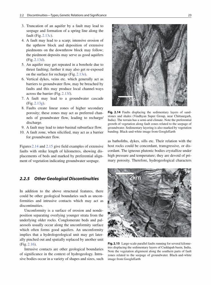
Figures 2.14 and 2.15 give field examples of extensive faults with strike length of kilometres, showing dis-placements of beds and marked by preferential align-ment of vegetation indicating groundwater seepage.

2.2.5 Other Geological Discontinuities

In addition to the above structural features, there could be other geological boundaries such as uncon-formities and intrusive contacts which may act as discontinuities.

Unconformity is a surface of erosion and nonde-position separating overlying younger strata from the underlying older rocks. Conglomerate beds and pal-aeosols usually occur along the unconformity surface which often forms good aquifers. An unconformity implies that a hydrologeological unit may get later-ally pinched out and spatially replaced by another unit (Fig. 2.16).

Intrusive contacts are other geological boundaries of significance in the context of hydrogeology. Intru-sive bodies occur in a variety of shapes and sizes, such

as batholiths, dykes, sills etc. Their relation with the host rocks could be concordant, transgressive, or dis-cordant. The igneous plutonic bodies crystallize under high pressure and temperature; they are devoid of pri-mary porosity. Therefore, hydrogeological characters

Fig. 2.14 Faults displacing the sedimentary layers of sand-stones and shales (Vindhyan Super Group, near Chittaurgarh, India). The terrain has a semi-arid climate. Note the preferential growth of vegetation along fault zones related to the seepage of groundwater. Sedimentary layering is also marked by vegetation banding. Black-and-white image from GoogleEarth

Fig. 2.15 Large-scale parallel faults running for several kilome-tres displacing the sedimentary layers of Cuddapah basin, India. Note the vegetation alignment along the southern parts of fault zones related to the seepage of groundwater. Black-and-white image from GoogleEarth


of the host rocks and intrusive rocks may be vastly dif-ferent from each other. Hence, igneous contacts act as regional boundaries from a hydrogeological point of view.

2.3 Fracture Characterization and Measurements

A fractured rock mass can be considered to be made up of three basic components: (a) fracture network, (b) matrix block and (c) infillings along the fractures, if present (see Fig. 2.1). A single fracture or disconti-nuity plane is characterised by its orientation, genetic nature (shear/tensile), persistence and aperture etc. Several fracture planes of the same type create a frac-ture set. They have certain spacing (frequency). Sev-eral intersecting intercommunicating fracture sets create a fracture network which facilitates fluid flow. Thus, it is extremely important to characterize discon-

tinuities and make their measurements, for a meaning-ful application. The various important parameters are summarised in Table 2.1.

The concept of Representative Elementary Volume (REV) is very important and may be introduced here. REV is the minimum rock mass volume which has the hydraulic and or mechanical properties similar to those of the rock mass. For mechanical properties, a sample size of a few cubic meters may be sufficient for approaching a REV; however, in case of hydraulic flow, REV may be substantially larger, and in some cases, it may not even exist due to strong anisotropy and spatial variability of rock characters.

2.3.1 Number of Sets

Several sets of discontinuities are often developed in a rock mass, three to four sets being most common. Number of sets of discontinuities in a exposure can be statistically determined by contouring the pole-plots (see Fig. 2.18). Relevant data as orientation, spacing, length, aperture etc. has to be collected for each set of discontinuity.

2.3.2 Orientation

Orientation is the parameter to define a single fracture plane in space, using angular relationships, as for any

Table 2.1 Parameters for discontinuity characterization

Parameter Description

1. Number of sets Number of sets of discontinuities present in the network 2. Orientation Attitude of discontinuity present in the network 3. Spacing Perpendicular distance between adjacent discontinuities of the same set 4. Persistence Trace length of the discontinuity seen in exposure 5. Density

– linear– areal– volumetric

Number of fractures per unit lengthCumulative length of fractures per unit area of exposureCumulative fractured surface area per unit bulk rock volume

6. Fracture area and shape Area of fractured surface and its shape 7. Volumetric fracture count Number of fractures per cubic metre of rock volume 8. Matrix block unit Block size and shape resulting from the fracture network 9. Connectivity Intersection and termination characteristics of fractures 10. Aperture Perpendicular distance between the adjacent rock-walls of a discontinuity, the space being air

or water-filled11. Asperity Projections of the wall-rock along the discontinuity surface12. Wall coatings and infillings Solid materials occurring as wall coatings and filling along the discontinuity surface

Fig. 2.16 Development of an aquifer along an unconformity between two impervious beds A and B

Unconformity

B

A

�.� Fracture Characterization and Measurements ��

geological planar surface. It is defined in terms of dip direction (angle with respect to north) and dip amount (angle with horizontal). The orientation is expressed in terms of a pair of numbers, such as 25°/N 330°, imply-ing a plane dipping at 25° in the direction 330° mea-sured clock-wise from the north. In field, inaccuracies often creep-in the measurements, and therefore statis-tical analysis is desirable.

Rose diagram is a method of displaying the relative statistical prevalence of various directional trends, e.g. strike direction of fractures, lineaments etc. It can be prepared for parameters such as number or length, i.e. number of joints direction-wise, or length of joints direc-tion-wise. Frequently, the directions are grouped in 10° interval. Frequency in a group-interval is represented along the radial axis, the length of petals becoming a measure of relative dominance of the trend. The strike petals possess a mirror image about the centre of the rosette. Data on the magnitude of dip cannot be incorpo-rated in the rosette, and may however be shown outside the circumference (Fig. 2.17). Histogram plot is another way to represent the relative prevalence of the trends.

Spherical projection: For representing orientation of geological planar surfaces, the method of stereographic equal-area projection is frequently employed, as it accu-rately shows the spatial distribution of data. Basic con-cepts on great-circle plots and π-pole plots to represent planes can be found in any standard text on structural geology (e.g. Billings 1972; Price and Cosgrove 1990). The method of plotting pole has a relative advantage over the great-circle method in that clusters of poles and their relative concentrations can be readily ascertained

on such plots by contouring. Schmidts-net is often used for density contouring to provide information on high-est concentration, i.e. the most dominant fracture plane. Figure 2.18 gives an example.

It may be important to find the over-all effect of various discontinuities. The mean direction of a group of poles can be represented by a simple vector-sum of all the constituting poles, following Fisher distri-bution. Similarly a resultant vector can be calculated

Fig. 2.17 Rose diagram of strike trends of discontinuities show-ing their relative prevalence

N

Fig. 2.18 a Orientation data of discontinuities. S0 is bedding plane, T1 and T2 are tensile fractures and S1 and S2 are shear fractures. Their great-circle and π-pole diagrams are shown in figures (b) and (c) respectively

Sr.No.

Surface Strike Dip direction Dip amount

ES0 N - S

N - S

N 338°

N 202° 80°

80°

45°

45°

N 68°-N 248°

N 112°-N 292°

E - W

1

2

3

4

5 S2

S1

T2

T1 –

T2 S0

N

S1

S2

T1

Great circle diagramFracture orientation dataa b c

N

S2

S0 T2

S1

π-Pole diagram

T1

W

Vertical


by summing all the clusters, to give a net directional effect of all the sets of discontinuities (Fig. 2.19).

It may be mentioned here that only selected and not all of the discontinuities present may play a significant role in fluid movement in the rock mass. Therefore, selection and data integration ought to be done judi-ciously. Further, Sharp (1993) gave a more useful con-cept for integration of discontinuity trend, frequency and aperture data to make hydraulic zonation maps (see Sect. 7.2.5).

2.3.3 Spacing (Interval)

Systematic joints are roughly equidistant and possess parallelism, and therefore, the parameter statistical

spacing has significance. It describes the average (or modal) perpendicular distance between two adjacent discontinuities of the same set. It has a profound influ-ence on rock mass permeability and groundwater flow. Fracture spacing is reciprocal of the fracture frequency or linear fracture density. It also controls fracture inten-sity and matrix block size.

Fracture separation ( fs) is related to lithology and thickness of the bed ( b), and is given as (Price and Cosgrove 1990):

fs = Y · b (2.1)

where Y is a constant related to lithology. Modelling and theoretical approaches also show that fracture spacing and bed thickness should have a linear rela-tionship, for a given lithologic material.

By spreading a tape in any convenient direction on an outcrop face, average apparent spacing ( fsa) between fractures of a set can be measured. This mea-surement has to be corrected for angular distortion (θ) to give the value of true fracture interval, perpendicu-lar to the fracture orientation. The correction angle (θ) equals the angle between the direction of tape align-ment and the pole to the fracture plane, and can be easily computed using a stereographic net (Fig. 2.20). The true fracture spacing ( fs) can be obtained from the measured fracture spacing ( fsa) as:

fs = fsa · cosθ (2.2)

Fig. 2.19 Principle of determining the mean pole direction as the resultant vector sum of all the vectors (poles), following Fisher method

Unit vector(pole)

Resultantsum vectorof all thepoles

Fig. 2.20 Spacing of frac-tures and computation of true fracture spacing. a Measure-ments in field for apparent fracture spacing. b Angle of correction, i.e. the angle between the line of tape align-ment and pole to the fracture plane, computed by stereo-graphic method

Tapelength L

Tape

Number offractures N

S

b

a T = Tape alignment

θ = Correction angle

P = Pole to the fracture plane

S–S = Great – circle of the outcrop face orientation

T

P

NS

Angle between tapealignment and normal to fracture plane = θ

Normal tofracture plane

Apparent fracture spacing = L / N = dmTrue fracture spacing = dm cos θ

θ


Further, it has been reported that fairly reliable esti-mates of fracture spacing can also be given by the P-wave velocity using seismic refraction techniques (see Sect. 5.6).

2.3.4 Persistence (Fracture Length)

Fracture persistence or length is a measure of the extent of development of discontinuity surface (Fig. 2.21). This carries the notion of size and controls the degree of fracturing. It is a crude measure of the penetra-tion length of a fracture in a rock mass. Fracture trace length is also related to fractured surface area. As some of the discontinuities are more persistent and continu-ous than others, it becomes a very important parameter in controlling groundwater flow.

Persistence is rather difficult to quantify, as it would differ in the dip and strike directions. It can be mea-sured by observing the discontinuity trace length in an exposure, in both dip and strike directions.

The observed trace length may be only an appar-ent value of the true trace length due to various types of bias creeping in the data during measurements in exposures, drifts, excavations, benches etc. For exam-ple, the biases could be like: (a) inability to recognize fracture traces shorter than a certain threshold length will lead to a bias (truncation of the histogram); (b) inability to measure full length of the traces owing to incomplete exposures in drift-walls, excavations etc. will lead to recording of censored length data; (c) the observed length of fracture trace depends on the relative orientation between the fracture plane and the exposure face; (d) in the sampling area or scanline, a stronger discontinuity is more likely to appear than a weaker one. Considering such aspects, methods for estimating the true trace length are discussed by a few workers (e.g. Pahl 1981; Laslett 1982; Chiles and de Marsily 1993).

2.3.5 Fracture Density

Fracture density is measured for each set of fracture set separately and corresponds to the degree of rock frac-turing. It can be described in three ways: linear, areal and volumetric, depending upon whether the measure-ment/computation corresponds to length (1D), area (2D) or volume (3D) aspect, respectively.

1. Linear fracture density (1D fracture density, d1) is the average number of fractures of a particular set, per unit length measured in a direction perpendicu-lar to the fracture plane. It equals fracture frequency (Ff) and is the reciprocal of fracture spacing.

2. Areal fracture density (2D fracture density, d2) is a way to quantify persistence of the discontinuity. It is the average fractured length (of traces) per unit area on a planar surface.

3. Volumetric fracture density (3D fracture density, d3) is the average fractured surface area per unit rock volume, created by all the fractures of a given set.

All types of fracture densities, d1, d2, and d3 have the same dimension (L−1). The volumetric density ( d3) is independent of direction and is a static parameter, like porosity. On the other hand, areal and linear densities are directional parameters and have bearing on fluid flow.

Both d1 and d2 depend on the orientation of the fractures vis-à-vis that of the scanline/exposure face. However, d3 is independent of direction and can be estimated from a survey with boreholes or scanlines, with the help of proper weighting of the observed fractures (Chiles and de Marsily 1993). For comput-ing the correct weighting factors, consider first the case of a borehole or a scanline survey (Fig. 2.22). The surveyed straight line can be considered as a cyl-inder of length L with a small section p, as in the case of a borehole. If n fractures intersect the survey line and ii is the acute angle made by the ith fracture plane with the borehole, then the fracture surface within the

Fig. 2.21 Influence of per-sistence of discontinuity on the degree of fracturing and interconnectivity Strong Moderate Weak


cylinder is p/sinii, for the ith fracture. Hence, 3D frac-ture density d3 is:

d3 =1

L · p

n

i=1

p

sinθi=

1

L

n

i=1

1

sinθi

(2.3)

Thus, the weighting factor is related to the acute angle between the fracture plane and the scanline.

Similarly, considering the case of an areal survey, the exposure can be considered as a layer of area S and a small thickness e. Within the surveyed rectangle, if n fractures are traced on the exposure (Fig. 2.23), and ith fracture has a trace length li and makes an angle ii with the exposure plane, then the fractured surface area for the ith fracture is e·li/sinii. Hence, 3D fracture density is:

d3 =1

S · e

n

i=1

e · lisin θi

=

1

S

n

i=1

lisin θi

(2.4)

Thus, the weighting factor is related to acute angle and fracture trace length. If all the fractures have the same trace length, then l is constant. For parallel fractures, ii can be replaced by i. For example, in an area in Bun-delkhand granites (India), the 3D fracture density was computed using the scanline method at 64 observation sites. It is observed that d3 in the area varies generally from about 6 m−1 to 21 m−1, whereas there are smaller pockets of higher values of d3, of the order of 31 m−1. The variation in d3 across the study area is shown in Fig. 2.24, where the magnitude of d3 is plotted as a circle of appropriate radius.

With simplifications and assumptions, d1, d2 and d3 can be interrelated; if fracture orientations are purely random, then (Chiles and de Marsily 1993):

d1 = l/2 · d3 (2.5)

d2 = π/2 · d3 (2.6)

2.3.6 Fracture Area and Shape

Fracture area can be estimated from the strike trace length and dip trace length, assuming that the fractured surface has a certain regular shape, e.g. circular, square, elliptical, rectangular or polygonal. Out of these the case of circular discs is the simplest. Disc diameter D can be related to fracture surface area A as:

A = (π/4) ·

�D2 + S2

D

(2.7)

where SD is the standard deviation of disc diameter distribution. Statistical aspects on the bearing of frac-ture shape on area estimation are discussed by a few workers (e.g. Lee and Farmer 1993). The 3D density of disc centres τ, average disc surface area A and the 3D fracturation density d3 are interrelated as:

d3 = τ × A (2.8)

2.3.7 Volumetric Fracture Count

Volumetric fracture count ( Vf) is the total number of fractures per cubic meter (m3) of rock volume and is determined from the mean fracture spacing as:

Vf = 1/fs1 + 1/fs2 + 1/fs3 · · · + 1/fsi (2.9)Fig. 2.23 Areal method of discontinuity survey

Plan

Sample area

Fig. 2.22 Scanline method of discontinuity survey

Section Drift face

Scanline

1


where fsi is the mean fracture spacing of the ith fracture set in metres. This also carries the notion of fracture intensity which is defined as the number of disconti-nuities per unit length, measured along a line, area or volume. Volumetric fracture count has a direct bear-ing on the size of matrix blocks and the representative elementary volume (REV).

2.3.8 Matrix Block Unit

The rock block bounded by fracture network is called matrix block unit. Each matrix block unit can be con-sidered to be hydrogeologically separated from the adjacent block. The shape of the matrix block unit could be prismatic, cubical or tabular, as governed by the orientation of fractures and their distribution (Fig. 2.25). For example, predominantly vertical frac-tures produce columnar and parellelopiped blocks (e.g. columnar joints in basalts); dominantly horizon-tal joints lead to plates and sheets (e.g. sheeting joints in granitoid rocks). These features impart hydraulic anisotropy to the geologic unit.

Consider an ideal case where beds are horizontal and fractures only vertical. It is known that fracture spacing and bed thickness are directly related (Eq. 2.1). It follows that a particular lithology has a tendency to develop block units of a certain shape, the block unit volume being dependent upon the bed thickness.

Block size is also related to the volumetric fracture count Vf. The maximum number of matrix blocks Nbmax can be expressed as (Kazi and Sen 1985):

Nbmax =

Vf

3+ 1

3

(2.10)

Fractal concepts are also used to define fragmented rocks. It is found that for fragmented materials includ-ing rocks, there is a size-frequency relationship of the form:

N (r) ∝

�r−D

(2.11)

where N( r) is the number of fragments with a charac-teristic linear dimension greater than ( r) and D is the

Fig. 2.24 Map showing variation in 3D fracture den-sity in a part of Bundelkhand granites, Central India

78°

25°30′20′

25′25°

78° 25′

N3D Fracture density

1 cm radius = 10 m–1

0 1 2 km

Fig. 2.25 Shape of matrix block units: prismatic, cubical and tabular

Prismatic

Cubical

Tabular

�0 � Fractures and Discontinuities

fractal dimension. It is believed that in future, fractal dimensions could be very useful in defining rock mass characteristics (e.g. Mojtabai et al. 1989; Ghosh 1990).

2.3.9 Fracture Connectivity

Discontinuities may exhibit differing termination and connectivity characteristics (Fig. 2.26a). Intersection of discontinuities is important as groundwater flow takes place through multiple fractures. Greater contin-uous inter-communication among the fracture network is provided by a higher degree of fracturing. Fracture connectivity increases with increasing fracture length and fracture density, as the chance of fracture intersec-tion increases.

For evaluating connectivity it is necessary to study how the fractures terminate. Barton et al. (1987) clas-sified fractures into three categories: abutting, crossing, and blind. The fractures of blind type do not intersect other fractures and remain unconnected. Laubach (1992) suggested that in many cases fracture connectivity may be gradual and that many fractures earlier classified as abutting, were really diffuse (interfingering type). He grouped fracture terminations into blind, diffuse and con-nected (which includes abutting). The data can be plot-ted in a ternary diagram to represent the bulk condition of fracture intersection in the rock mass (Fig. 2.26b). As an example, it is shown in the figure that most the joints in Bundelkhand granites (BG) are of connected type.

2.3.10 Rock Quality Designation (RQD)

RQD is a semi-quantitative measure of fracture den-sity which can be estimated from core recovery data.

RQD is defined as the ratio of the recovered core more than 4 in. (about 10 cm) long and of good quality to the total drilled length and is expressed as a percent-age. Although RQD is mainly used in assessing the geomechanical properties of rocks, it is also consid-ered to be an important parameter in assessing relative permeability.

2.3.11 Aperture

Aperture is the perpendicular distance separating the adjacent rockwalls of an open discontinuity, in which the intervening space is air or water-filled. Aperture may vary from very tight to wide. Commonly, subsur-face rock masses have small apertures. Tensile stress may lead to larger apertures or open fractures. Often shear fractures have much lower aperture values than the tensile fractures.

Aperture may increase by dissolution, erosion etc. particularly in the weathered zone. It may decrease with depth due to lithostatic pressure, and there frac-ture wall compression strength is an important param-eter governing aperture as lithostatic pressure tends to close the fracture opening. Table 2.2 gives aperture ranges as usually classified in rock mechanics.

Fracture aperture can be measured by various methods which include feeler gauge, flourescent dyes, impression packer, tracer test, hydraulic test etc. Readers may refer to Indraratna and Rajnith (2001) for details of various methods used for measurement of fracture aperture. Often, measurement of aperture in surface exposures is made with a vernier caliper or gauge and the measured opening is termed as the mechanical aperture. In the laboratory, fracture aper-ture can be estimated by impregnating rock samples

Fig. 2.26 Fracture connec-tivity. a Different types of fracture terminations: B blind; C crossing; D dif-fusely connected. b Ternary diagram of fracture termina-tions (After Laubach 1992); the point BG corresponds to data from Bundelkhand gran-ites indicating high degree of fracture interconnectivity

BB

B

B

DD

DDC

C

DD

B

C

B B C B

B

Diffuse Connected

BG

Blind

a b

�.� Methods of Field Investigations ��

with dyes or resin and by studying the thin sections under the microscope. This method can even be used in soft sediments viz. clay till (Klint and Rosenbem 2001). Lerner and Stelle (2001) have suggested two field techniques to estimate the in-situ spatial varia-tion of fracture aperture: one is the conventional slug hydraulic testing using packers and in the second tech-nique NAPL (sunflower oil) is injected into isolated fractures in a borehole.

The term ‘equivalent aperture’ is introduced to account for the variation in fracture which can be esti-mated from tracer test and hydraulic tests. The terms ‘tracer aperture’ and ‘hydraulic aperture’ are intro-duced by Tsang (1999) depending on the method of estimation. The hydraulic aperture is estimated from hydraulic tests based on the Cubic Law:

Tf ∝ a3 (2.12)

where a is the fracture aperture and Tf is the transmis-sivity of the formation (also see Sect. 7.2.1).

The data on discontinuity sets with corresponding apertures is to be recorded. Asperities affect the aper-ture size and also render its measurement difficult in field. Therefore, when considering fluid flow, apertures are defined in terms of flow properties, as volumetric flow rate is governed by the cube of aperture. Aperture can be integrated with fracture density to give an inte-grated function representative of hydraulic conductiv-ity (see Sect. 7.2.5).

2.3.12 Asperity

Fracture walls are not flat parallel smooth surfaces but contain irregularities, called asperities (Fig. 2.27). The asperity reduces fluid flow and leads to a local chan-nelling effect of preferential flow. This reduces the

effective porosity and makes flow velocities irregular. Observations on asperities should be made for each type of fracture surface and measurement made. Mean height of asperities together with Reynolds number Re has a direct influence on flow regime, i.e. laminar vs. turbulent flow (Sect. 7.1.1).

2.3.13 Wall Coatings and Infillings

It is the solid material occurring between the adjacent walls of a discontinuity, e.g. clay, fault gouge, breccia, chert, calcite, etc. Filling material could be homoge-neous or heterogeneous, and could partly or completely fill the discontinuity. The material may have variable permeability, depending upon mineralogy, grain size, width etc. The net effect of wall coatings and infillings is a reduced aperture.

2.4 Methods of Field Investigations

Methods of field investigations can be classified into two broad types (Jouanna 1993): 2D and 3D (Table 2.3). The 2D methods are based on observations made at rock surface, at surface or subsurface lev-els. They include scanline surveys, borehole surveys, and different types of areal surveys (Fig. 2.28). These methods give an idea of the hydrogeological properties at and around the site of observation.

The 3D methods are aimed at gathering information on the bulk volumetric properties involving inner struc-ture of the fractured rock mass. There can be direct or indirect 3D methods. Brief descriptions of the various 2D and 3D methods are given below.

Table 2.2 Aperture classification by size. (After Barton 1973)

Aperture (mm) Term

<0.1 Very tight0.1–0.25 Tight0.25–0.50 Partly open0.50–2.50 Open2.50–10.0 Moderately wide>10.0 Wide

Fig. 2.27 Asperities in fracture walls

Asperities

Aperture


2.4.1 Scanline Surveys

Scanline surveys involve direct observation of rock features along a line on the rock surface, e.g. on an out-crop, drift face, excavation, adit etc. (Fig. 2.22). Scan-lines are usually horizontal; however, vertical scanlines are preferred where fractures are mostly horizontal. Data on fractures obtained by sampling techniques such as along scanline (and also borehole) are strongly biased towards the fractures oriented perpendicular to the scanline/core and needs to be corrected for sam-pling bias by applying correction (Terzaghi 1965).

A suitable rock exposure or face is selected. A sam-ple scanline is marked on the face, and its orientation (rake on the face) is recorded. Fractures intersecting the line are collected. Each fracture is represented by its trace which can be measured. Observations are made for various parameters, like: location of the fracture trace intersection with the scanline; orientation of the fracture and angle made with the scanline; termination type if seen and connectivity; alternatively, whether the

fracture extends beyond the top of face/batter; fracture type and other relevant fracture characteristics.

2.4.2 Areal Surveys

Areal surveys can be treated as extension of the scan-line surveys. They are used for surveying fracture char-acteristics on a rock surface area, e.g. on an outcrop, drift face, adit, tunnel etc. (Fig. 2.23). In field, an area is first demarcated on a rock surface for observation and statistical sampling. Detailed observations on frac-ture characteristics are made with-in the marked area where all the fractures data are collected.

Direct observations and field mapping at natural rock outcrops is an old established technique. Weath-ering, surficial cover, soil, vegetation etc. influence the accessibility and visibility of good outcrops. Excava-tions, pits and trenches are made to expose the fresh rocks at shallow depth for visual inspection. Subsur-face direct observation can be made in adits and tun-

Fig. 2.28 The various 2D methods of field investigations

Pit

Outcrop

Boreholes

Tunnel/mine

Table 2.3 Methods of field investigations

1. 2D Methods—Based on rock surface observations on lithology, structure, fractures, and their characteristics; made at surface or subsurface levels

1.1 Scanline surveys1.2 Areal surveys—on outcrops, pits, trenches, adits, drift etc. including terrestrial geophotogrammetry and remote sensing1.3 Borehole surveys—including drilling, study of oriented cores, borehole logging, dipmeter, borehole cameras and formation

microscanner methods2. 3D Method—Investigations aimed at bulk volumetric properties of rock mass in 3D

2.1 Hydraulic well tests2.2 Hydrochemical methods2.3 Geophysical methods including seismic, electrical, EM, gravity, magnetic and georadar

Further Reading ��

nels. Geological maps of rock faces exposed can be prepared and fracture characteristics measured.

Remote sensing includes study of photographs and images acquired from aerial and space platforms. This technique can give valuable information on geol-ogy, structure, fractures, lineaments etc. and forms an important mapping tool (Chap. 4). Further, stereo-photographs of rocks exposed in outcrops, scarps, excavations, etc. can be taken from a ground-based (terrestrial) platform. These stereo pairs can be studied and measurements of fracture characteristics can be done in laboratory.

2.4.3 Borehole Surveys

These are the only tools for direct observations of rock surface and features occurring at depth. A number of methods are available. As drilling is expensive, opti-mum combination of methods is employed for getting maximum information from drilling. In the case of ver-tical and sub-vertical fractures, inclined bores are pre-ferred to intercept a number of such fractures. Study of drill cores, particularly oriented drill cores provides data on orientation of structures, fractures, their apertures as well as infillings. Further, borehole walls can be studied in several ways. Geophysical well logging is a standard technique, including electrical, caliper, radioactivity, magnetic logging etc. These give information on lithol-ogy and structure. Borehole televiewer provides images of the borehole walls with joints and fractures. Dipme-ter and formation microscanner help measure orienta-tion of structural features at depth in-situ (for drilling and well observation techniques, see Chap. 5).

It may be mentioned here again that data on frac-tures obtained by sampling techniques such as along scanline and borehole are strongly biased towards the fractures oriented perpendicular to the core/scanline and needs to be corrected for sampling bias by apply-ing a correction (Terzaghi 1965).

2.4.4 3D Methods

As mentioned above, 3D methods are aimed to pro-vide information on bulk volumetric properties of

the fractured rock mass. These methods include hydraulic well tests, hydrochemical methods and geophysical techniques. The hydraulic well tests comprise pumping tests of various configurations and types, and give bulk volumetric assessment. Slug tests will give a first hand dependable information about the hydraulic conductivity at much lower costs than pumping tests (see Chap. 9). In hydrochemical methods various types of geochemical tracer studies and solute transport studies are carried out for bulk volumetric hydrogeological characterization (see Sect. 10.3). Further, a number of geophysical meth-ods are used such as seismic, electrical, EM, gravity, magnetic and georadar. They are briefly described in Chap. 5 from a hydrogeological investigation point of view.

SummaryMost rocks possess fractures, broadly termed as discontinuities here, which facilitate storage and movement of fluids through the medium The discontinuities may be formed by planar sur-faces such as bedding plane, foliation, fractures, faults shear zones etc. The common system-atic fractures are of three main genetic origins: extensional, shear and hybrid. Faults can cause truncation or repetition aquifers and may lead to formation of springs and interbasinal subsurface flow. Discontinuities are characterized in terms of a number of parameters such as orientation, spac-ing, persistence, fracture and shape, connectivity, aperture coatings etc., and these data may be col-lected from field surveys by scanline method or areal surveys or in borehole observations.

Further Reading

Billings MP (1972) Structural Geology. 3rd ed., Prentice Hall, New Delhi, 606 p.

Lee CH, Farmer I (1993) Fluid Flow in Discontinuous Rocks. Chapman and Hall, London, 169 p.

Marshak S, Mitra G (2006) Basic Methods of Structural Geol-ogy. 2nd ed., Prentice Hall, New Jersey, 446 p.

van Golf-Racht TD (1982) Fundamentals of Fractured Reservoir Engineering. Elsevier, Amsterdam, 710 p.

http://www.springer.com/978-90-481-8798-0

fractures and discontinuities

Documents