ABAQUS

Tutorial

Version 5

Fracture Analysis Consultants, Inc

www.fracanalysis.com

Revised: September 2010

1

Table of Contents:

1.0 Introduction .......................................................................................................................... 2

2.0 Tutorial 1: Crack Insertion and Growth in a Cube .............................................................. 2 2.1 Step 1: Creating the ABAQUS Model ............................................................................ 3 2.2 Step 2: FRANC3D Crack Insertion and Analysis ........................................................... 9

3.0 Tutorial 2: Center Through-Crack in a Plate Sub-Domain ................................................ 23 3.1 Step 1: Creating the uncracked model using ABAQUS ............................................... 24

3.2 Step 2: Crack insertion and remeshing with FRANC3D .............................................. 30 3.3 Step 3a: Merging the cracked, local part with the global part using FRANC3D and

analysis using ABAQUS........................................................................................................... 35

3.4 Step 3b: Merging the cracked, local part with the global part in ABAQUS and analysis

using ABAQUS ........................................................................................................................ 38 3.5 Step 4: Calculate fracture parameters using FRANC3D ............................................... 42

4.0 Tutorial 3: Automated Crack Growth in a Plate, with Crack Face Tractions ................... 43 4.1 Step 1: Creating the uncracked model using ABAQUS ............................................... 43

4.2 Step 2: Crack insertion with FRANC3D ....................................................................... 47 4.3 Step 3: Applying crack face traction ............................................................................. 51 4.4 Step 4: Automated crack growth analyses .................................................................... 53

2

1.0 Introduction

This manual contains tutorials that introduce the modeling capabilities available through the

interface of FRANC3D Version 5 and ABAQUS Version 6.6 (or later). The first tutorial

describes a model where the entire domain is remeshed during crack insertion and crack growth.

The second tutorial describes a model where only a local subdomain is remeshed during crack

insertion and growth. The second tutorial provides somewhat more detailed instructions for the

ABAQUS portion because of the increased modeling effort. The third tutorial describes the

process of applying crack face tractions along with the process of automated crack growth. It is

intended that the user perform the operations as they are presented, but you should feel free to

experiment and consult the other reference documentation whenever necessary.

Menu and dialog box selections are indicated by bold text, such as File. Model and

corresponding file names will be indicated by italic text and window names and window regions

are underlined. So, selections that need to be made are indicated by bold text and the windows

and regions of windows where these selections are made are underlined.

2.0 Tutorial 1: Crack Insertion and Growth in a Cube

This tutorial contains an example for FRANC3D with ABAQUS 6.6. The capabilities of the

program are illustrated by analyzing a surface crack in a simple component (a cube). Note that

the ABAQUS CAE user interface generally changes with each new version, so the images of

icons or the menu layout might be different if you are using later versions (6.7 - 6.10).

First, all the steps needed to create the model geometry using ABAQUS are briefly described in

Section 2.1. It is assumed that the user is somewhat familiar with ABAQUS. Once the model is

created in ABAQUS, the FRANC3D steps necessary to read the mesh information, insert a

crack, rebuild the mesh, perform the ABAQUS analysis, and compute stress intensity factors are

described in Section 2.2.

3

Note that ABAQUS generally provides a number of different ways to access menu and dialog

entries; you can use your favorite shortcuts or follow the tutorial.

2.1 Step 1: Creating the ABAQUS Model

First, we create a cube model using ABAQUS. We assume that the user knows how to use

ABAQUS, but we provide enough details in the steps below for a novice user to create the

simple cube model.

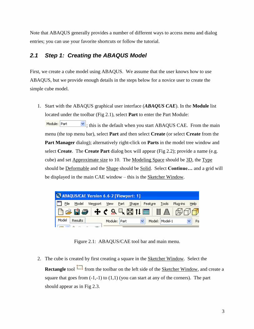
1. Start with the ABAQUS graphical user interface (ABAQUS CAE). In the Module list

located under the toolbar (Fig 2.1), select Part to enter the Part Module:

; this is the default when you start ABAQUS CAE. From the main

menu (the top menu bar), select Part and then select Create (or select Create from the

Part Manager dialog); alternatively right-click on Parts in the model tree window and

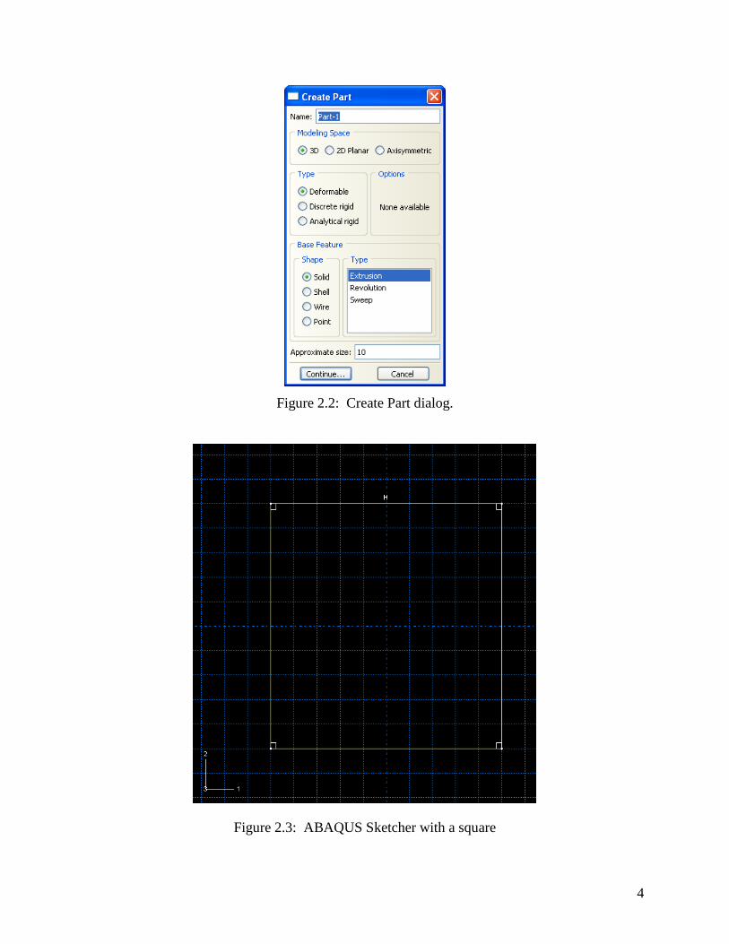
select Create. The Create Part dialog box will appear (Fig 2.2); provide a name (e.g.

cube) and set Approximate size to 10. The Modeling Space should be 3D, the Type

should be Deformable and the Shape should be Solid. Select Continue… and a grid will

be displayed in the main CAE window – this is the Sketcher Window.

Figure 2.1: ABAQUS/CAE tool bar and main menu.

2. The cube is created by first creating a square in the Sketcher Window. Select the

Rectangle tool from the toolbar on the left side of the Sketcher Window, and create a

square that goes from (-1,-1) to (1,1) (you can start at any of the corners). The part

should appear as in Fig 2.3.

4

Figure 2.2: Create Part dialog.

Figure 2.3: ABAQUS Sketcher with a square

5

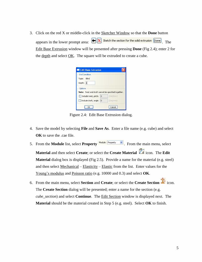
3. Click on the red X or middle-click in the Sketcher Window so that the Done button

appears in the lower prompt area: . The

Edit Base Extrusion window will be presented after pressing Done (Fig 2.4); enter 2 for

the depth and select OK. The square will be extruded to create a cube.

Figure 2.4: Edit Base Extrusion dialog.

4. Save the model by selecting File and Save As. Enter a file name (e.g. cube) and select

OK to save the .cae file.

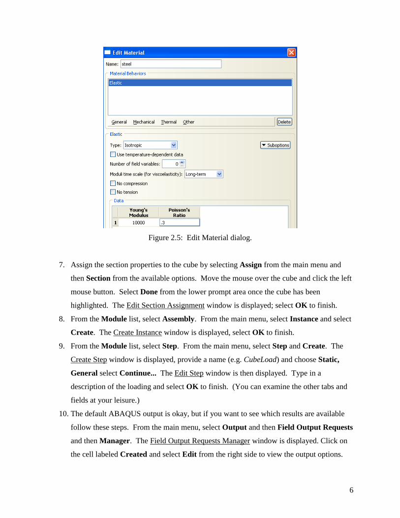
5. From the Module list, select Property . From the main menu, select

Material and then select Create; or select the Create Material icon. The Edit

Material dialog box is displayed (Fig 2.5). Provide a name for the material (e.g. steel)

and then select Mechanical – Elasticity – Elastic from the list. Enter values for the

Young‟s modulus and Poisson ratio (e.g. 10000 and 0.3) and select OK.

6. From the main menu, select Section and Create; or select the Create Section icon.

The Create Section dialog will be presented; enter a name for the section (e.g.

cube_section) and select Continue. The Edit Section window is displayed next. The

Material should be the material created in Step 5 (e.g. steel). Select OK to finish.

6

Figure 2.5: Edit Material dialog.

7. Assign the section properties to the cube by selecting Assign from the main menu and

then Section from the available options. Move the mouse over the cube and click the left

mouse button. Select Done from the lower prompt area once the cube has been

highlighted. The Edit Section Assignment window is displayed; select OK to finish.

8. From the Module list, select Assembly. From the main menu, select Instance and select

Create. The Create Instance window is displayed, select OK to finish.

9. From the Module list, select Step. From the main menu, select Step and Create. The

Create Step window is displayed, provide a name (e.g. CubeLoad) and choose Static,

General select Continue... The Edit Step window is then displayed. Type in a

description of the loading and select OK to finish. (You can examine the other tabs and

fields at your leisure.)

10. The default ABAQUS output is okay, but if you want to see which results are available

follow these steps. From the main menu, select Output and then Field Output Requests

and then Manager. The Field Output Requests Manager window is displayed. Click on

the cell labeled Created and select Edit from the right side to view the output options.

7

Select OK or Cancel to close the Edit dialog and then select Dismiss to finish with the

Output Request Manager.

11. From the Module list, select Load. From the main menu, select Load and Create. The

Create Load window is displayed. Provide a name and choose Pressure and select

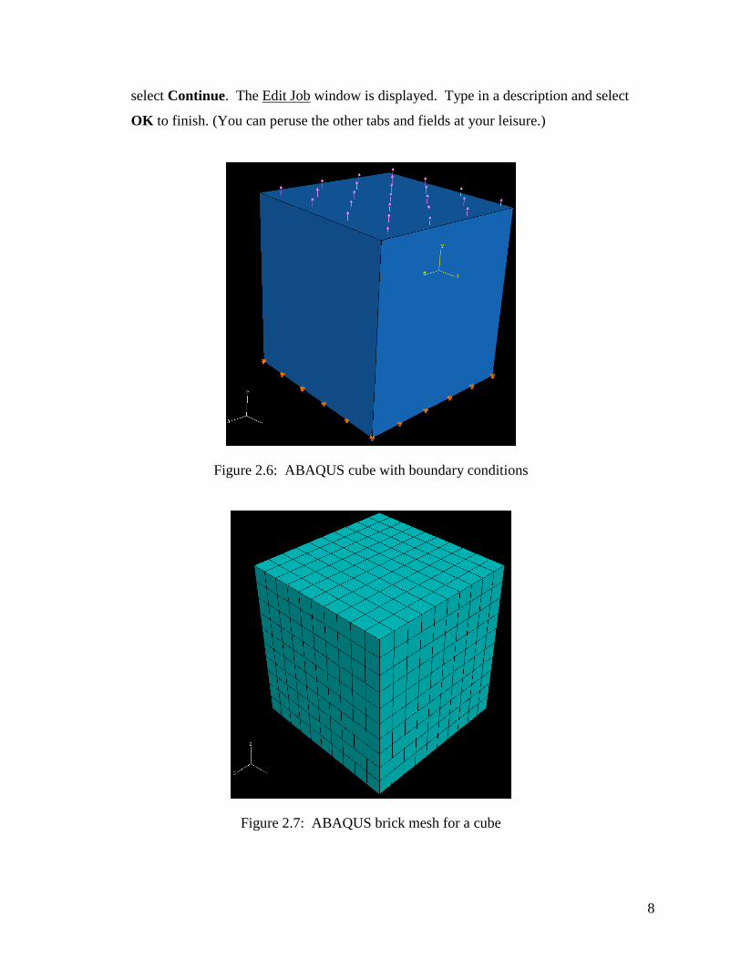
Continue. Pick the top surface of the cube and select Done from the lower prompt area.

The Edit Load window is displayed; set the uniform pressure magnitude to be -1.0. The

resulting model should appear as in Fig 2.6; the symbols for the boundary conditions are

shown.

12. From the Module list, select Load (if you changed modules after Step 11). From the

main menu, select BC and then select Create. The Create Boundary Condition window

is displayed. Provide a name and choose Symmetry/Antisymmetry/Encastre and select

Continue. Pick the bottom face of the cube and select Done from the lower prompt area;

you will need to rotate the model to see the bottom face. The Edit Boundary Condition

window will be presented, choose PINNED and select OK. The boundary condition

symbols are shown on the model.

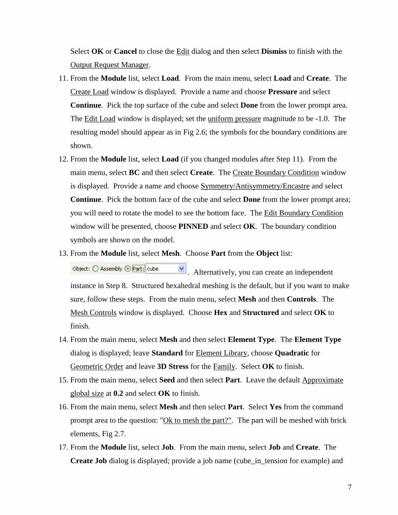
13. From the Module list, select Mesh. Choose Part from the Object list:

. Alternatively, you can create an independent

instance in Step 8. Structured hexahedral meshing is the default, but if you want to make

sure, follow these steps. From the main menu, select Mesh and then Controls. The

Mesh Controls window is displayed. Choose Hex and Structured and select OK to

finish.

14. From the main menu, select Mesh and then select Element Type. The Element Type

dialog is displayed; leave Standard for Element Library, choose Quadratic for

Geometric Order and leave 3D Stress for the Family. Select OK to finish.

15. From the main menu, select Seed and then select Part. Leave the default Approximate

global size at 0.2 and select OK to finish.

16. From the main menu, select Mesh and then select Part. Select Yes from the command

prompt area to the question: "Ok to mesh the part?". The part will be meshed with brick

elements, Fig 2.7.

17. From the Module list, select Job. From the main menu, select Job and Create. The

Create Job dialog is displayed; provide a job name (cube_in_tension for example) and

8

select Continue. The Edit Job window is displayed. Type in a description and select

OK to finish. (You can peruse the other tabs and fields at your leisure.)

Figure 2.6: ABAQUS cube with boundary conditions

Figure 2.7: ABAQUS brick mesh for a cube

9

Special Note: Click on the tab below the Modeling Window (at the very bottom) and type:

mdb.models['model_name'].setValues(noPartsInputFile=ON)

where „model_name‟ is the actual model name you are using, and then press “Enter”.

This is required because FRANC3D doesn‟t read Parts.

18. From the main menu, select Job and Manager. The Job Manager window is displayed.

Select Submit on the right side. The analysis will start and should complete successfully.

Select the Results option on the right side to view the results.

19. Save the model using the File and Save As menu options. Note that a number of files

will be created automatically as ABAQUS runs. Included in the set of files should be an

.inp file with the Job name as the prefix. This is the file that will be read by FRANC3D.

This initial analysis provides baseline results and ensures that we have created a correct

model.

Note that the purpose of Steps 18 and 19 is not merely to create the .inp file that FRANC3D

requires, but to perform an analysis and look at the results to make sure the displacement and

stress results are as expected. You can skip these steps and simply Write Input by right-

clicking on the job name under Analysis and Jobs in the model tree window. Don‟t forget to

save the .cae model file in case you wish to return to this model and modify properties, etc.

You can Exit from ABAQUS CAE now.

2.2 Step 2: FRANC3D Crack Insertion and Analysis

We need to start with a pre-existing mesh for FRANC3D. We will use the .inp file created by

ABAQUS during Step 1.19.

1. Start with the FRANC3D graphical user interface, Fig 2.8, and select File and Open.

2. Switch File Filter in the Open Model File window, Fig 2.9, to Abaqus Files (*.inp) and

select the file name for the model, called cube.inp here. Select OK or double click on the

file name. The next set of wizard panels allows you to choose the data that will be

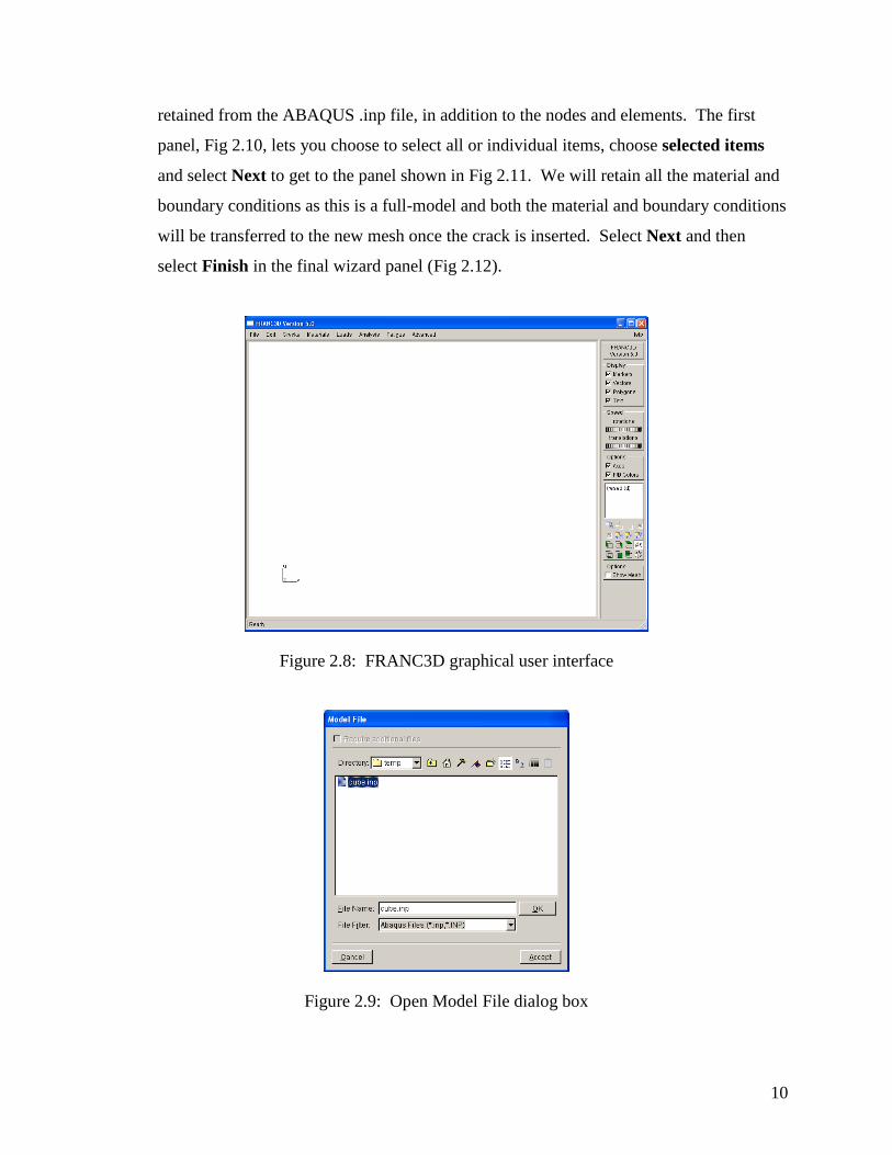
10

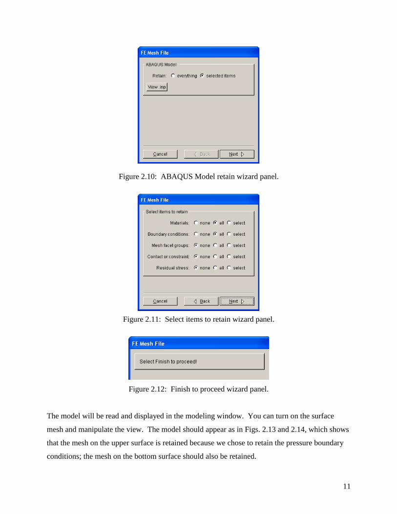
retained from the ABAQUS .inp file, in addition to the nodes and elements. The first

panel, Fig 2.10, lets you choose to select all or individual items, choose selected items

and select Next to get to the panel shown in Fig 2.11. We will retain all the material and

boundary conditions as this is a full-model and both the material and boundary conditions

will be transferred to the new mesh once the crack is inserted. Select Next and then

select Finish in the final wizard panel (Fig 2.12).

Figure 2.8: FRANC3D graphical user interface

Figure 2.9: Open Model File dialog box

11

Figure 2.10: ABAQUS Model retain wizard panel.

Figure 2.11: Select items to retain wizard panel.

Figure 2.12: Finish to proceed wizard panel.

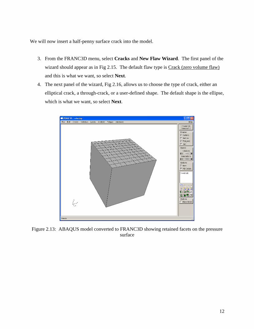
The model will be read and displayed in the modeling window. You can turn on the surface

mesh and manipulate the view. The model should appear as in Figs. 2.13 and 2.14, which shows

that the mesh on the upper surface is retained because we chose to retain the pressure boundary

conditions; the mesh on the bottom surface should also be retained.

12

We will now insert a half-penny surface crack into the model.

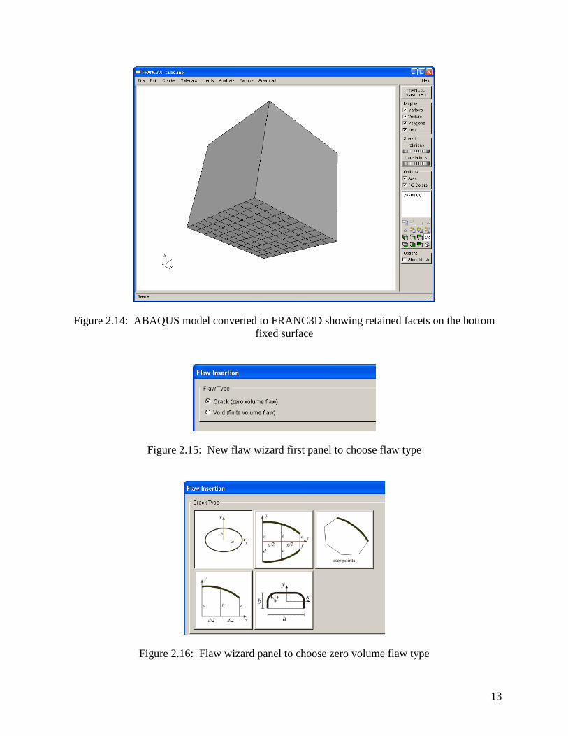
3. From the FRANC3D menu, select Cracks and New Flaw Wizard. The first panel of the

wizard should appear as in Fig 2.15. The default flaw type is Crack (zero volume flaw)

and this is what we want, so select Next.

4. The next panel of the wizard, Fig 2.16, allows us to choose the type of crack, either an

elliptical crack, a through-crack, or a user-defined shape. The default shape is the ellipse,

which is what we want, so select Next.

Figure 2.13: ABAQUS model converted to FRANC3D showing retained facets on the pressure

surface

13

Figure 2.14: ABAQUS model converted to FRANC3D showing retained facets on the bottom

fixed surface

Figure 2.15: New flaw wizard first panel to choose flaw type

Figure 2.16: Flaw wizard panel to choose zero volume flaw type

14

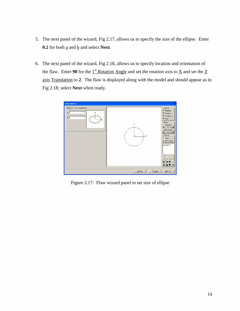
5. The next panel of the wizard, Fig 2.17, allows us to specify the size of the ellipse. Enter

0.2 for both a and b and select Next.

6. The next panel of the wizard, Fig 2.18, allows us to specify location and orientation of

the flaw. Enter 90 for the 1st Rotation Angle and set the rotation axis to X and set the Z

axis Translation to 2. The flaw is displayed along with the model and should appear as in

Fig 2.18; select Next when ready.

Figure 2.17: Flaw wizard panel to set size of ellipse

15

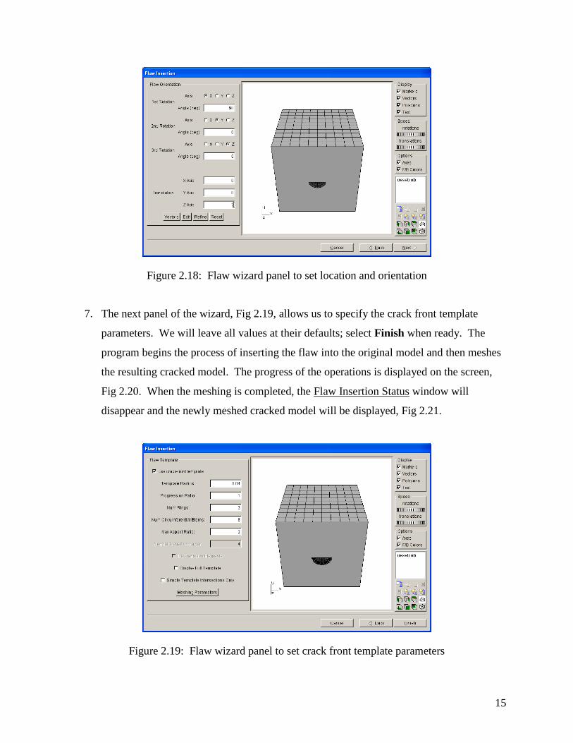
Figure 2.18: Flaw wizard panel to set location and orientation

7. The next panel of the wizard, Fig 2.19, allows us to specify the crack front template

parameters. We will leave all values at their defaults; select Finish when ready. The

program begins the process of inserting the flaw into the original model and then meshes

the resulting cracked model. The progress of the operations is displayed on the screen,

Fig 2.20. When the meshing is completed, the Flaw Insertion Status window will

disappear and the newly meshed cracked model will be displayed, Fig 2.21.

Figure 2.19: Flaw wizard panel to set crack front template parameters

16

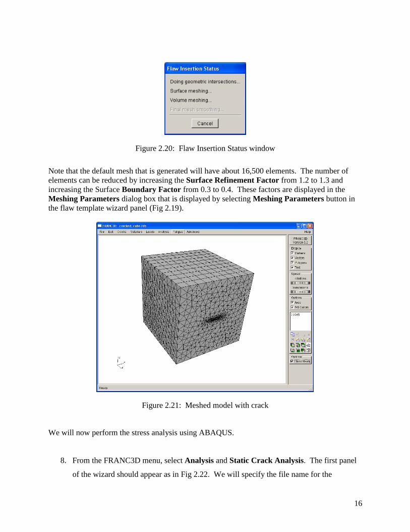
Figure 2.20: Flaw Insertion Status window

Note that the default mesh that is generated will have about 16,500 elements. The number of

elements can be reduced by increasing the Surface Refinement Factor from 1.2 to 1.3 and

increasing the Surface Boundary Factor from 0.3 to 0.4. These factors are displayed in the

Meshing Parameters dialog box that is displayed by selecting Meshing Parameters button in

the flaw template wizard panel (Fig 2.19).

Figure 2.21: Meshed model with crack

We will now perform the stress analysis using ABAQUS.

8. From the FRANC3D menu, select Analysis and Static Crack Analysis. The first panel

of the wizard should appear as in Fig 2.22. We will specify the file name for the

17

FRANC3D database first. We called it cracked_cube.fdb here; select Next once you

enter a File Name.

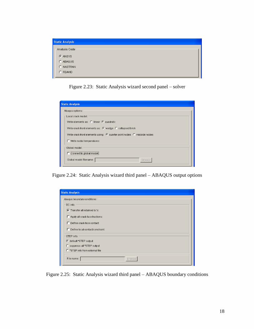
9. The next panel of the wizard, Fig 2.23, allows us to specify the solver; choose ABAQUS.

10. The next panel of the wizard, Fig 2.24, allows us to specify some of the ABAQUS output

options. We want to use all quadratic elements, we do not have nodal temperatures, and

the model is a full-model and will NOT be combined with a global model; uncheck the

Connect to global model and select Next.

11. The next panel of the wizard, Fig 2.25, allows us to specify the boundary conditions.

This is a full model and we will transfer all boundary conditions from the original model

to the crack model; the other options should remain unchecked.

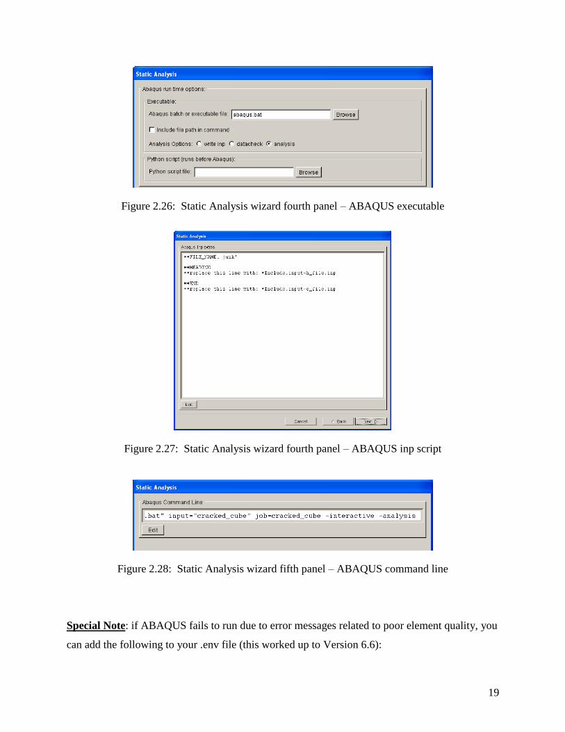
12. The next panel of the wizard, Fig 2.26, allows us to specify the ABAQUS executable. If

you wish to only check the data in the resulting .inp file, choose datacheck. Select Next.

13. The next panel of the wizard, Fig 2.27, allows us to add additional ABAQUS commands

to the .inp file. Select Next.

14. The final panel of the wizard, Fig 2.28, displays the command line that will be used to

invoke ABAQUS. The line can be edited. Select Finish when ready. If ABAQUS is

available and the settings are correct, ABAQUS should start in batch mode. If ABAQUS

fails to start, the command line is saved in a .txt file and can be used to start the analysis

outside of FRANC3D (from a cmd/terminal window). You should check the FRANC3D

terminal window for the runtime status.

If you cannot run ABAQUS from FRANC3D, then you will have to submit your job from a

cmd/terminal window before proceeding to step 15.

Figure 2.22: Static Analysis wizard first panel – File Name

18

Figure 2.23: Static Analysis wizard second panel – solver

Figure 2.24: Static Analysis wizard third panel – ABAQUS output options

Figure 2.25: Static Analysis wizard third panel – ABAQUS boundary conditions

19

Figure 2.26: Static Analysis wizard fourth panel – ABAQUS executable

Figure 2.27: Static Analysis wizard fourth panel – ABAQUS inp script

Figure 2.28: Static Analysis wizard fifth panel – ABAQUS command line

Special Note: if ABAQUS fails to run due to error messages related to poor element quality, you

can add the following to your .env file (this worked up to Version 6.6):

20

import os

os.environment['ABA_SKIPSTRICTGEOMCHECK']='YES'

del os

We will now compute the stress intensity factors for this crack. If you are able to run ABAQUS

from FRANC3D, then the model already exists and the displacement file will be read

automatically and you can skip to Step 16.

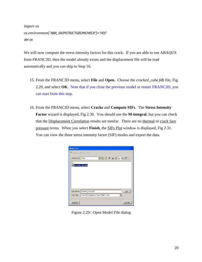
15. From the FRANC3D menu, select File and Open. Choose the cracked_cube.fdb file, Fig

2.29, and select OK. Note that if you close the previous model or restart FRANC3D, you

can start from this step.

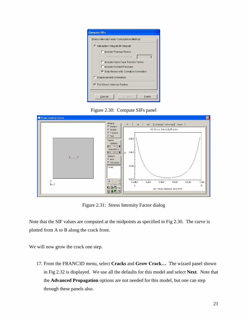
16. From the FRANC3D menu, select Cracks and Compute SIFs. The Stress Intensity

Factor wizard is displayed, Fig 2.30. You should use the M-integral, but you can check

that the Displacement Correlation results are similar. There are no thermal or crack face

pressure terms. When you select Finish, the SIFs Plot window is displayed, Fig 2.31.

You can view the three stress intensity factor (SIF) modes and export the data.

Figure 2.29: Open Model File dialog

21

Figure 2.30: Compute SIFs panel

Figure 2.31: Stress Intensity Factor dialog

Note that the SIF values are computed at the midpoints as specified in Fig 2.30. The curve is

plotted from A to B along the crack front.

We will now grow the crack one step.

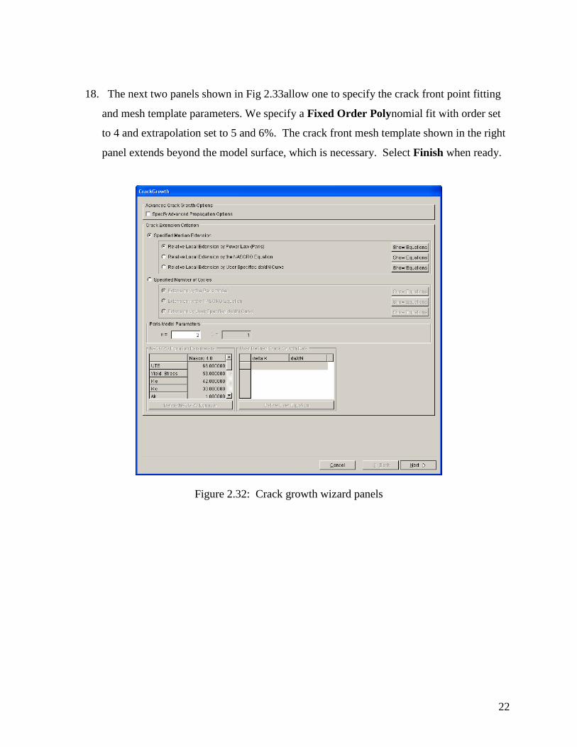
17. From the FRANC3D menu, select Cracks and Grow Crack… The wizard panel shown

in Fig 2.32 is displayed. We use all the defaults for this model and select Next. Note that

the Advanced Propagation options are not needed for this model, but one can step

through these panels also.

22

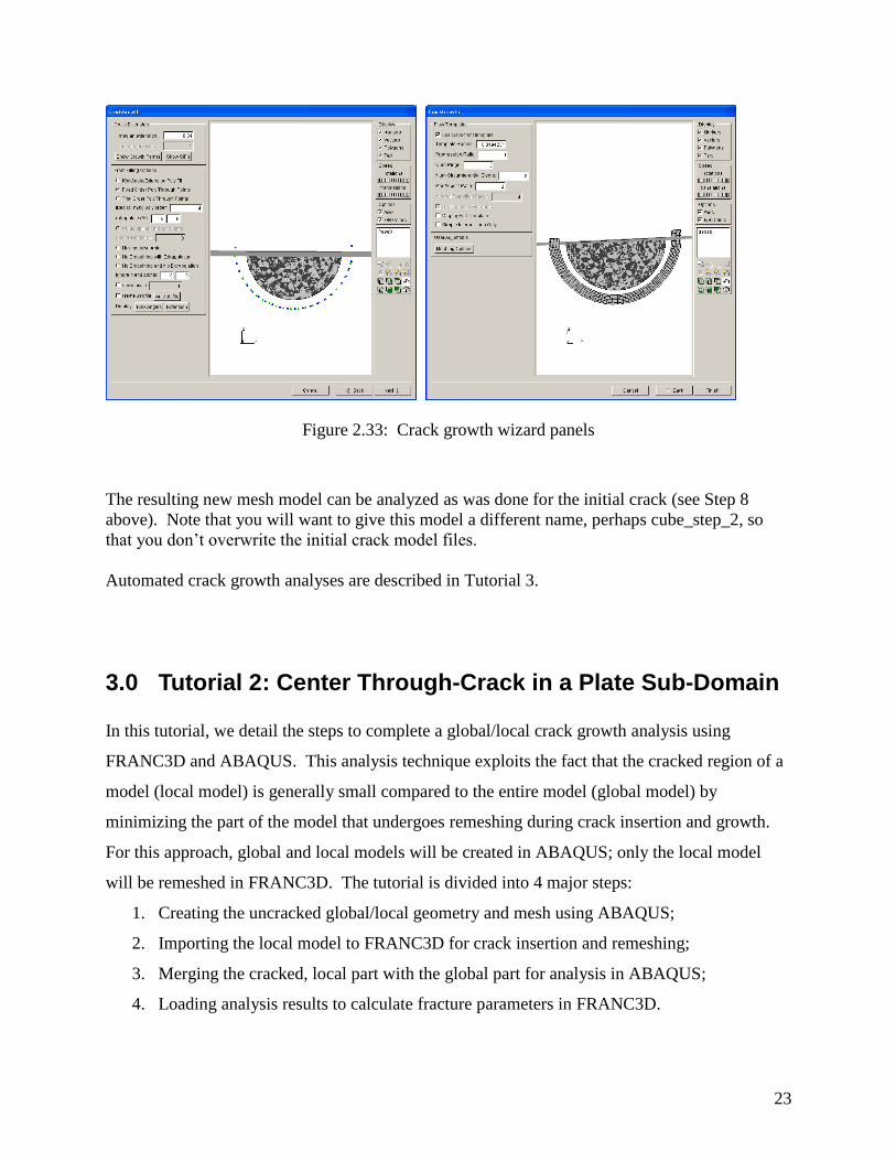
18. The next two panels shown in Fig 2.33allow one to specify the crack front point fitting

and mesh template parameters. We specify a Fixed Order Polynomial fit with order set

to 4 and extrapolation set to 5 and 6%. The crack front mesh template shown in the right

panel extends beyond the model surface, which is necessary. Select Finish when ready.

Figure 2.32: Crack growth wizard panels

23

Figure 2.33: Crack growth wizard panels

The resulting new mesh model can be analyzed as was done for the initial crack (see Step 8

above). Note that you will want to give this model a different name, perhaps cube_step_2, so

that you don‟t overwrite the initial crack model files.

Automated crack growth analyses are described in Tutorial 3.

3.0 Tutorial 2: Center Through-Crack in a Plate Sub-Domain

In this tutorial, we detail the steps to complete a global/local crack growth analysis using

FRANC3D and ABAQUS. This analysis technique exploits the fact that the cracked region of a

model (local model) is generally small compared to the entire model (global model) by

minimizing the part of the model that undergoes remeshing during crack insertion and growth.

For this approach, global and local models will be created in ABAQUS; only the local model

will be remeshed in FRANC3D. The tutorial is divided into 4 major steps:

1. Creating the uncracked global/local geometry and mesh using ABAQUS;

2. Importing the local model to FRANC3D for crack insertion and remeshing;

3. Merging the cracked, local part with the global part for analysis in ABAQUS;

4. Loading analysis results to calculate fracture parameters in FRANC3D.

24

Although it is not explicitly stated in the steps below, make sure to SAVE your work throughout

the modeling process. In particular, save the .cae file throughout and at the end of Step 1. Also,

it is assumed that the user has some basic knowledge of ABAQUS. The unfamiliar user is

referred to “Getting Started With ABAQUS” (part of the ABAQUS documentation).

3.1 Step 1: Creating the uncracked model using ABAQUS

Start by creating a simple plate model using ABAQUS:

1. Open the ABAQUS CAE and select Create Model Database.

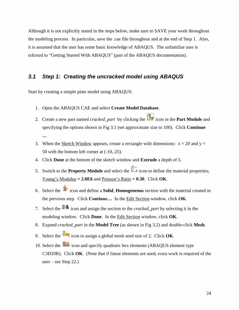
2. Create a new part named cracked_part by clicking the icon in the Part Module and

specifying the options shown in Fig 3.1 (set approximate size to 100). Click Continue

…

3. When the Sketch Window appears, create a rectangle with dimensions: x = 20 and y =

50 with the bottom left corner at (-10,-25).

4. Click Done at the bottom of the sketch window and Extrude a depth of 5.

5. Switch to the Property Module and select the icon to define the material properties;

Young‟s Modulus = 2.0E6 and Poisson‟s Ratio = 0.30. Click OK.

6. Select the icon and define a Solid, Homogeneous section with the material created in

the previous step. Click Continue… In the Edit Section window, click OK.

7. Select the icon and assign the section to the cracked_part by selecting it in the

modeling window. Click Done. In the Edit Section window, click OK.

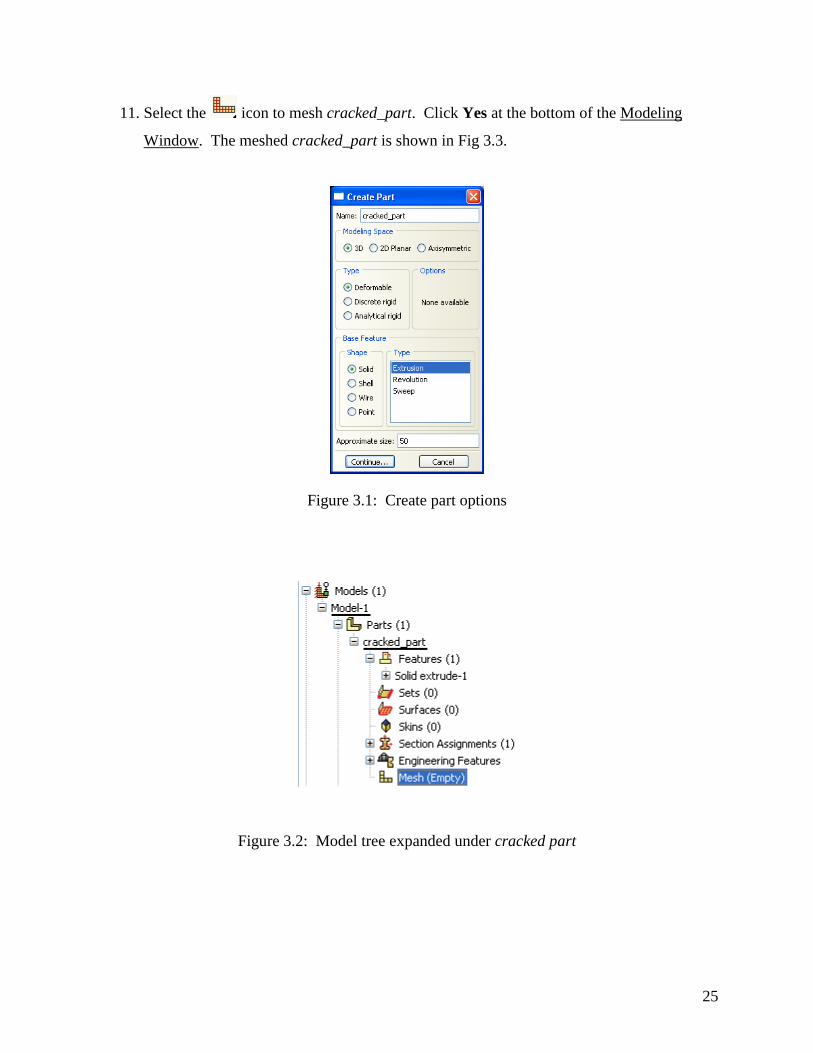
8. Expand cracked_part in the Model Tree (as shown in Fig 3.2) and double-click Mesh.

9. Select the icon to assign a global mesh seed size of 2. Click OK.

10. Select the icon and specify quadratic hex elements (ABAQUS element type

C3D20R). Click OK. (Note that if linear elements are used, extra work is required of the

user – see Step 22.)

25

11. Select the icon to mesh cracked_part. Click Yes at the bottom of the Modeling

Window. The meshed cracked_part is shown in Fig 3.3.

Figure 3.1: Create part options

Figure 3.2: Model tree expanded under cracked part

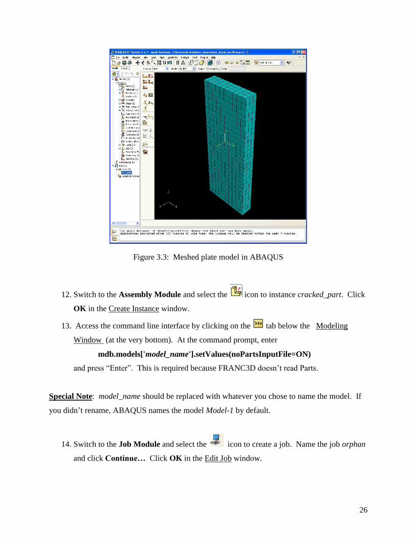
26

Figure 3.3: Meshed plate model in ABAQUS

12. Switch to the Assembly Module and select the icon to instance cracked_part. Click

OK in the Create Instance window.

13. Access the command line interface by clicking on the tab below the Modeling

Window (at the very bottom). At the command prompt, enter

mdb.models['model_name'].setValues(noPartsInputFile=ON)

and press “Enter”. This is required because FRANC3D doesn‟t read Parts.

Special Note: model_name should be replaced with whatever you chose to name the model. If

you didn‟t rename, ABAQUS names the model Model-1 by default.

14. Switch to the Job Module and select the icon to create a job. Name the job orphan

and click Continue… Click OK in the Edit Job window.

27

15. Select the icon to display the Job Manager. Select orphan and click Write Input at

the right. Click Dismiss.

Special Note: ABAQUS doesn‟t allow creation of node sets from a part created in CAE. We

need some node set definitions to inform FRANC3D which surfaces will be used to glue the

local model back into the global model so that the mesh on those surfaces will remain unaltered.

So, we must now read in the orphan mesh created in the previous steps to define the local and

global models.

16. From the File menu, select Import and Model and then select orphan.inp. Click OK.

17. A new model is created in the Model Tree at the left. Right click on the orphan model

and select Copy Model … and name the new model global. Click OK.

18. Repeat the previous step and name the copied model local. Click OK.

19. Switch to the Mesh Module, global Model, and Object: Part at the top of the modeling

window and select Mesh and Edit from the upper toolbar. In the Edit Mesh window,

select Element in the Category region and select Delete in the Method region.

Special Note: since the global model region is being defined first, the portion of the model that

will be used for local crack insertion needs to be deleted first.

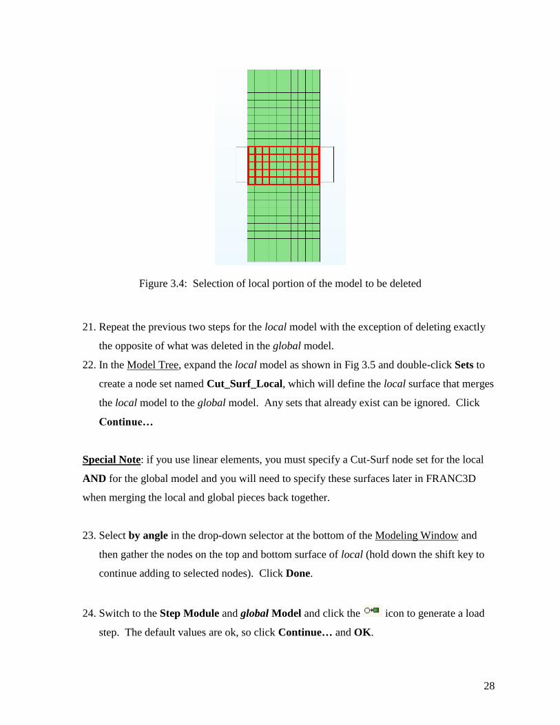
20. As shown in Fig 3.4, select the portion of the model that corresponds to the local model,

leaving only the global portion unselected (most easily done by viewing the 1-2 plane).

At the bottom of the Modeling Window, with Delete associated unreferenced nodes

selected, click Done. Switch to the Assembly Module, which will automatically

regenerate the instance.

28

Figure 3.4: Selection of local portion of the model to be deleted

21. Repeat the previous two steps for the local model with the exception of deleting exactly

the opposite of what was deleted in the global model.

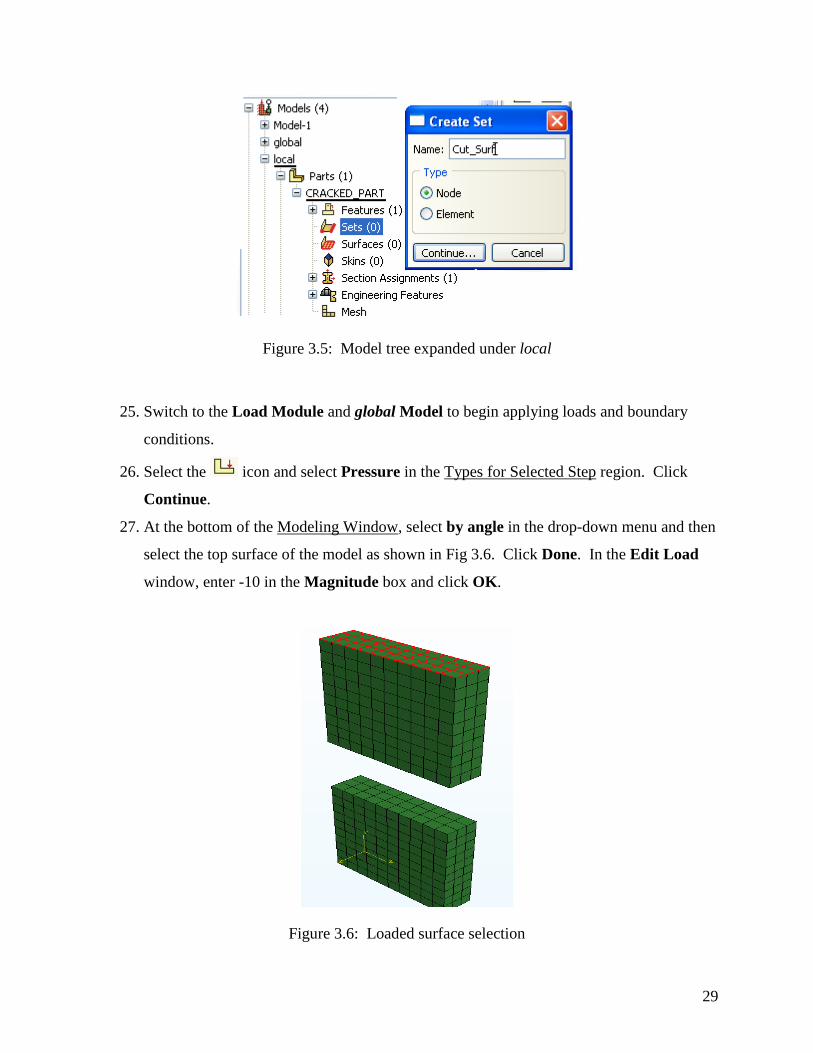
22. In the Model Tree, expand the local model as shown in Fig 3.5 and double-click Sets to

create a node set named Cut_Surf_Local, which will define the local surface that merges

the local model to the global model. Any sets that already exist can be ignored. Click

Continue…

Special Note: if you use linear elements, you must specify a Cut-Surf node set for the local

AND for the global model and you will need to specify these surfaces later in FRANC3D

when merging the local and global pieces back together.

23. Select by angle in the drop-down selector at the bottom of the Modeling Window and

then gather the nodes on the top and bottom surface of local (hold down the shift key to

continue adding to selected nodes). Click Done.

24. Switch to the Step Module and global Model and click the icon to generate a load

step. The default values are ok, so click Continue… and OK.

29

Figure 3.5: Model tree expanded under local

25. Switch to the Load Module and global Model to begin applying loads and boundary

conditions.

26. Select the icon and select Pressure in the Types for Selected Step region. Click

Continue.

27. At the bottom of the Modeling Window, select by angle in the drop-down menu and then

select the top surface of the model as shown in Fig 3.6. Click Done. In the Edit Load

window, enter -10 in the Magnitude box and click OK.

Figure 3.6: Loaded surface selection

30

28. Click the icon and rotate the model so that the bottom surface is visible. In the

Create Boundary Condition pop-up window enter: face_y for the Name, Step-1 for the

step, Mechanical in the Category region and Displacement/Rotation in the Types for

Selected Step region. Click Continue… With by angle selected at the bottom of the

Modeling Window, select the bottom face of the model. Click Done.

29. In the Edit Boundary Condition window, select U2 and enter 0. Click OK.

30. Once again, click the icon. In the Create Boundary Condition window enter:

point_xz for the Name, Step-1 for the step, Mechanical in the Category region and

Displacement/Rotation in the Types for Selected Step region. Click Continue… With

individual selected in the drop-down selector at the bottom of the Modeling Window,

select the middle node on the bottom face. Click Done.

31. In the Edit Boundary Condition window, select U1, U3 and enter 0 in both. Click OK.

32. Switch to the Job Module and select the icon to create a job. With global

highlighted, name the job global and click Continue… and OK. Repeat for local with

local highlighted in the Create Job window.

33. Select the icon to display the Job Manager. Select global and click Write Input at

the right. Repeat for local. Click Dismiss.

34. Before exiting ABAQUS CAE, save your work.

At this point in the tutorial, we have finished Step 1 in which the global and local portions of the

model have been defined. In the next step, we will use the local model for crack

insertion/remeshing in FRANC3D.

3.2 Step 2: Crack insertion and remeshing with FRANC3D

The next step is to read the local model into FRANC3D and insert a crack. We have saved the

two inp files as: local .inp and global .inp. Inside the local file, there is a node set called

Cut_Surf_Local that defines the nodes of the mesh facets in local that are to be retained.

1. Copy the local .inp and global .inp files from the ABAQUS working directory to the

FRANC3D working directory.

31

2. Start FRANC3D.

3. Select File and Open. In the Open Model File window, choose the Abaqus (*.inp) file

filter and select local.inp file and Click OK.

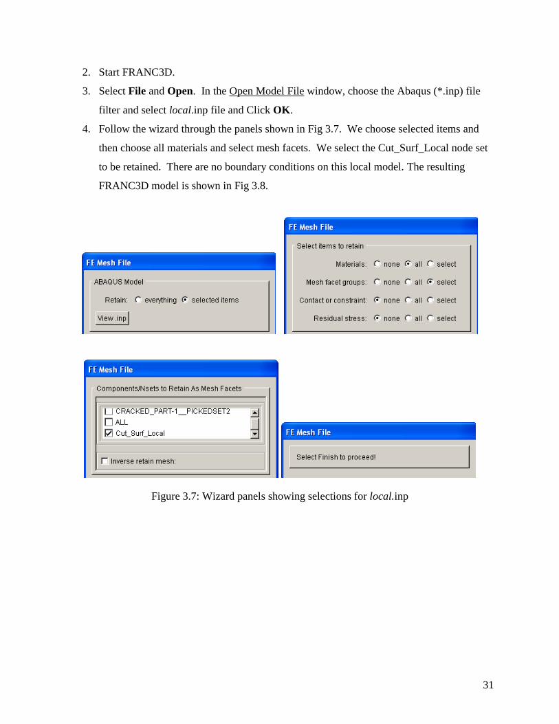
4. Follow the wizard through the panels shown in Fig 3.7. We choose selected items and

then choose all materials and select mesh facets. We select the Cut_Surf_Local node set

to be retained. There are no boundary conditions on this local model. The resulting

FRANC3D model is shown in Fig 3.8.

Figure 3.7: Wizard panels showing selections for local.inp

32

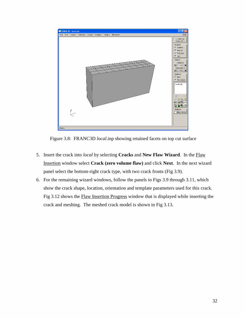
Figure 3.8: FRANC3D local.inp showing retained facets on top cut surface

5. Insert the crack into local by selecting Cracks and New Flaw Wizard. In the Flaw

Insertion window select Crack (zero volume flaw) and click Next. In the next wizard

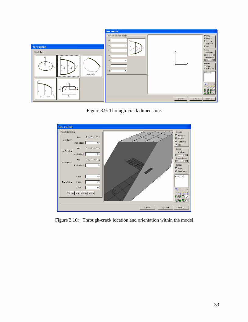
panel select the bottom-right crack type, with two crack fronts (Fig 3.9).

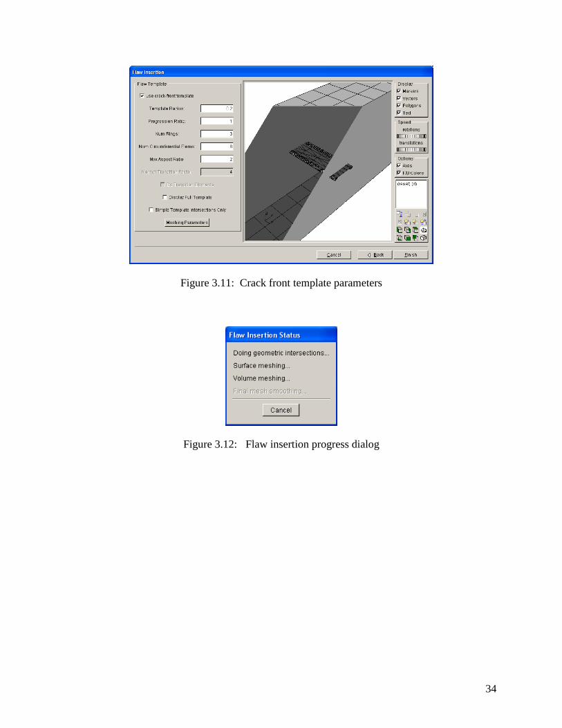
6. For the remaining wizard windows, follow the panels in Figs 3.9 through 3.11, which

show the crack shape, location, orientation and template parameters used for this crack.

Fig 3.12 shows the Flaw Insertion Progress window that is displayed while inserting the

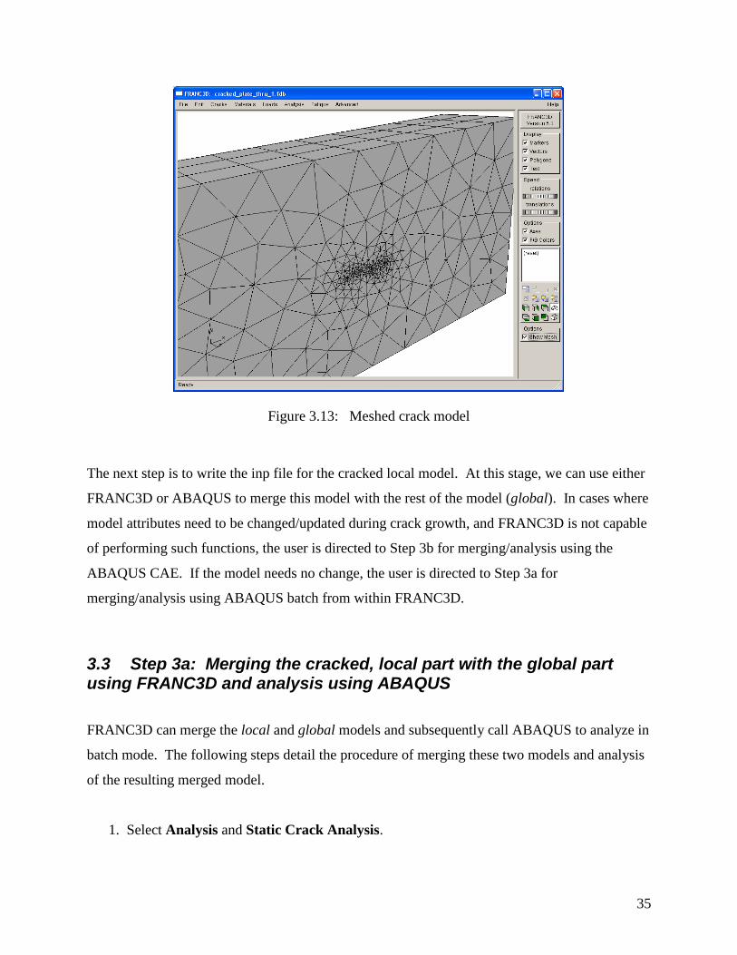
crack and meshing. The meshed crack model is shown in Fig 3.13.

33

Figure 3.9: Through-crack dimensions

Figure 3.10: Through-crack location and orientation within the model

34

Figure 3.11: Crack front template parameters

Figure 3.12: Flaw insertion progress dialog

35

Figure 3.13: Meshed crack model

The next step is to write the inp file for the cracked local model. At this stage, we can use either

FRANC3D or ABAQUS to merge this model with the rest of the model (global). In cases where

model attributes need to be changed/updated during crack growth, and FRANC3D is not capable

of performing such functions, the user is directed to Step 3b for merging/analysis using the

ABAQUS CAE. If the model needs no change, the user is directed to Step 3a for

merging/analysis using ABAQUS batch from within FRANC3D.

3.3 Step 3a: Merging the cracked, local part with the global part using FRANC3D and analysis using ABAQUS

FRANC3D can merge the local and global models and subsequently call ABAQUS to analyze in

batch mode. The following steps detail the procedure of merging these two models and analysis

of the resulting merged model.

1. Select Analysis and Static Crack Analysis.

36

2. Specify a file name in the first wizard panel (e.g. cracked_plate_00). Click Next.

Choose ABAQUS from the next wizard panel. Click Next.

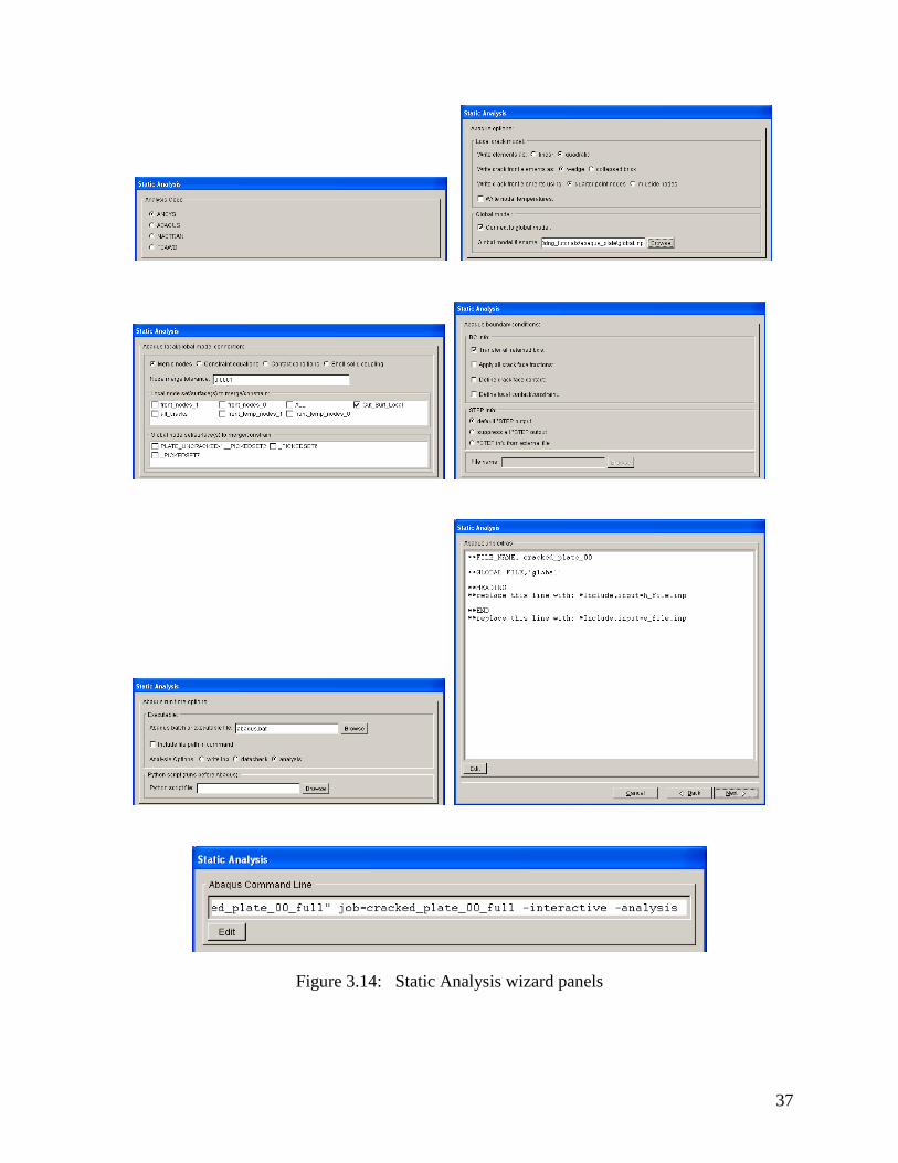
Step through the Analysis wizard as shown in Fig 3.14:

3. Choose to Connect to global model in the following wizard panel and specify global.inp

as the Global model filename. Click Next.

4. Choose to Merge local and global nodes and in Local node set/surface(s) to

merge/constrain, choose the Cut_Surf_Local node set. Ignore the Global node

set/surface(s) to merge/constrain box (as long as you used second-order elements). Click

Next.

5. There are no boundary conditions on the local model, but because we are merging with

the global model, we want to transfer all the boundary conditions from the original global

model to the new combined crack model, so leave the Transfer all retained bc‟s checked.

Click Next.

6. In the next panel, select the ABAQUS batch file if needed and make sure the analysis

button is pressed and click Next.

7. The next panel requires no changes for this model. Click Next.

8. The final panel displays the command line. Click Finish to begin the analysis of the

merged model. If the ABAQUS analysis fails to start from FRANC3D or if you need to

transfer the files to a different computer, you can run ABAQUS from a cmd/terminal

window using the .inp as input.

When the analysis has completed, proceed to Step 4. The following files are created by

FRANC3D: cracked_plate_00.fdb, cracked_plate_00.inp, cracked_plate_00_full.inp, and

cracked_plate_00.txt. The cracked_plate_00.inp must not be overwritten as this file corresponds

to the meshed crack model; the cracked_plate_00_full.inp corresponds to the merged model.

37

Figure 3.14: Static Analysis wizard panels

38

Note that if the analysis fails to run in ABAQUS due to errors associated with element volume

shape measures, you can redo the crack insertion and meshing after modifying the Meshing

Parameters. Or you can add the following to your .env file (this worked up to Version .6.6):

import os

os.environment['ABA_SKIPSTRICTGEOMCHECK']='YES'

del os

3.4 Step 3b: Merging the cracked, local part with the global part in ABAQUS and analysis using ABAQUS

If there is a need to modify the model in ABAQUS, we can merge the global and the cracked

version of local in ABAQUS CAE.

1. Select Analysis and Static Crack Analysis.

2. Specify a file name in the first wizard panel (e.g. cracked_plate_00). Click Next.

Choose ABAQUS from the next wizard panel. Click Next.

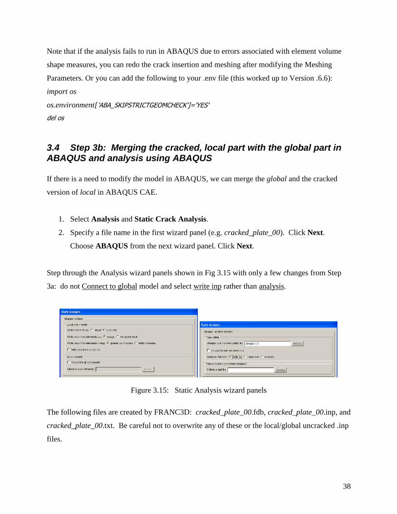
Step through the Analysis wizard panels shown in Fig 3.15 with only a few changes from Step

3a: do not Connect to global model and select write inp rather than analysis.

Figure 3.15: Static Analysis wizard panels

The following files are created by FRANC3D: cracked_plate_00.fdb, cracked_plate_00.inp, and

cracked_plate_00.txt. Be careful not to overwrite any of these or the local/global uncracked .inp

files.

39

NOTE: this section is not complete, you will have to manage section properties and

boundary conditions and parts on your own to get the model to run.

3. Open the ABAQUS CAE and select Open Model Database. Select the .cae file created

in Step 1.

4. In your working directory, make a copy of cracked_plate.inp and name it local_1.inp to

ensure we do not overwrite cracked_plate.inp.

5. From the File menu, select Import and Model and then select local_1.inp. Click OK.

This creates a new model in the Model Tree named local_1.

6. Expand local_1 in the Model Tree and then expand Parts. By default, ABAQUS named

the imported part Part-1; rename Part-1 by right-clicking on it and selecting Rename

and typing local_1 in the Rename Part window. Click OK.

7. Copy the global model to a new model named merged_1 by right-clicking on global and

selecting Copy… as was done in Step 1. Keeping global separate allows us to use it for

merging in subsequent crack growth steps.

8. From the Model menu, select Copy Objects… to merge merged_1 with local_1.

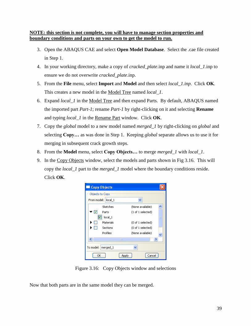
9. In the Copy Objects window, select the models and parts shown in Fig 3.16. This will

copy the local_1 part to the merged_1 model where the boundary conditions reside.

Click OK.

Figure 3.16: Copy Objects window and selections

Now that both parts are in the same model they can be merged.

40

10. Switch to the Assembly Module and merged_1 Model and select the icon to

instance the local_1 part. Click OK in the Create Instance window.

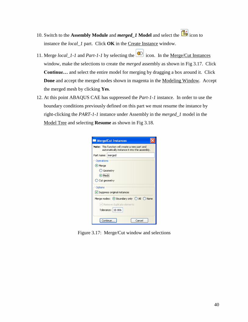
11. Merge local_1-1 and Part-1-1 by selecting the icon. In the Merge/Cut Instances

window, make the selections to create the merged assembly as shown in Fig 3.17. Click

Continue… and select the entire model for merging by dragging a box around it. Click

Done and accept the merged nodes shown in magenta in the Modeling Window. Accept

the merged mesh by clicking Yes.

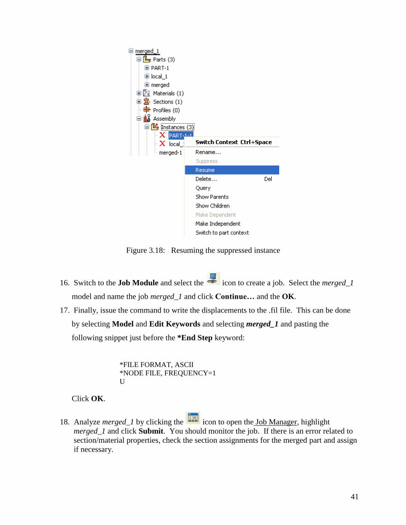
12. At this point ABAQUS CAE has suppressed the Part-1-1 instance. In order to use the

boundary conditions previously defined on this part we must resume the instance by

right-clicking the PART-1-1 instance under Assembly in the merged_1 model in the

Model Tree and selecting Resume as shown in Fig 3.18.

Figure 3.17: Merge/Cut window and selections

41

Figure 3.18: Resuming the suppressed instance

16. Switch to the Job Module and select the icon to create a job. Select the merged_1

model and name the job merged_1 and click Continue… and the OK.

17. Finally, issue the command to write the displacements to the .fil file. This can be done

by selecting Model and Edit Keywords and selecting merged_1 and pasting the

following snippet just before the *End Step keyword:

*FILE FORMAT, ASCII

*NODE FILE, FREQUENCY=1

U

Click OK.

18. Analyze merged_1 by clicking the icon to open the Job Manager, highlight

merged_1 and click Submit. You should monitor the job. If there is an error related to

section/material properties, check the section assignments for the merged part and assign

if necessary.

42

3.5 Step 4: Calculate fracture parameters using FRANC3D

1. Copy the ABAQUS generated .fil file to the FRANC3D directory, if it‟s not there

already. Note that you might want to rename the file to cracked_plate.fil.

2. Start FRANC3D and open the cracked_plate_00.fdb file saved during Step 3. Note that

you might have to select the cracked_plate_full.fil file manually.

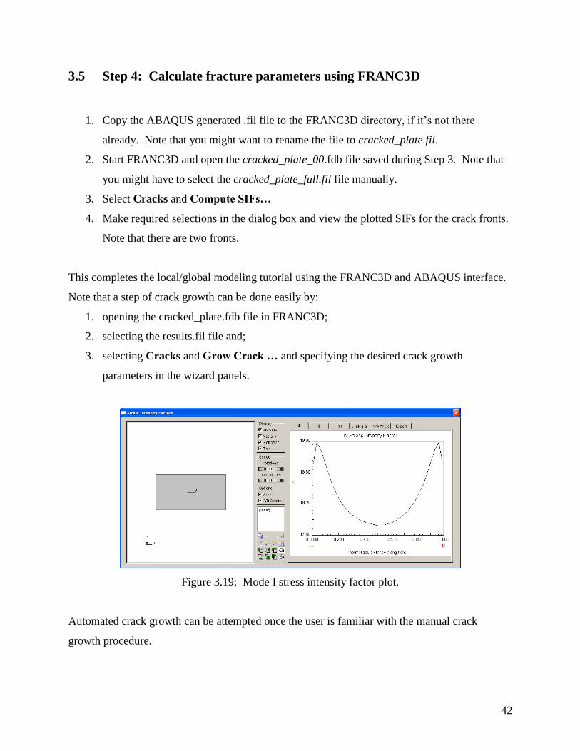
3. Select Cracks and Compute SIFs…

4. Make required selections in the dialog box and view the plotted SIFs for the crack fronts.

Note that there are two fronts.

This completes the local/global modeling tutorial using the FRANC3D and ABAQUS interface.

Note that a step of crack growth can be done easily by:

1. opening the cracked_plate.fdb file in FRANC3D;

2. selecting the results.fil file and;

3. selecting Cracks and Grow Crack … and specifying the desired crack growth

parameters in the wizard panels.

Figure 3.19: Mode I stress intensity factor plot.

Automated crack growth can be attempted once the user is familiar with the manual crack

growth procedure.

43

4.0 Tutorial 3: Automated Crack Growth in a Plate, with Crack Face Tractions

In this tutorial, we describe the steps to complete an automated crack growth analysis using the

FRANC3D and ABAQUS interface, including the application of crack face tractions from an

uncracked ABAQUS stress analysis. For this tutorial, an initial uncracked model will be created

and analyzed in ABAQUS. The tutorial is divided into 4 major steps:

1. Creating the uncracked geometry and mesh using ABAQUS;

2. Importing the model to FRANC3D for crack insertion and remeshing;

3. Applying the crack face tractions;

4. Static crack analysis and subsequent automatic crack growth analysis.

4.1 Step 1: Creating the uncracked model using ABAQUS

Start by creating a simple plate model using ABAQUS:

1. Open the ABAQUS CAE and select Create Model Database.

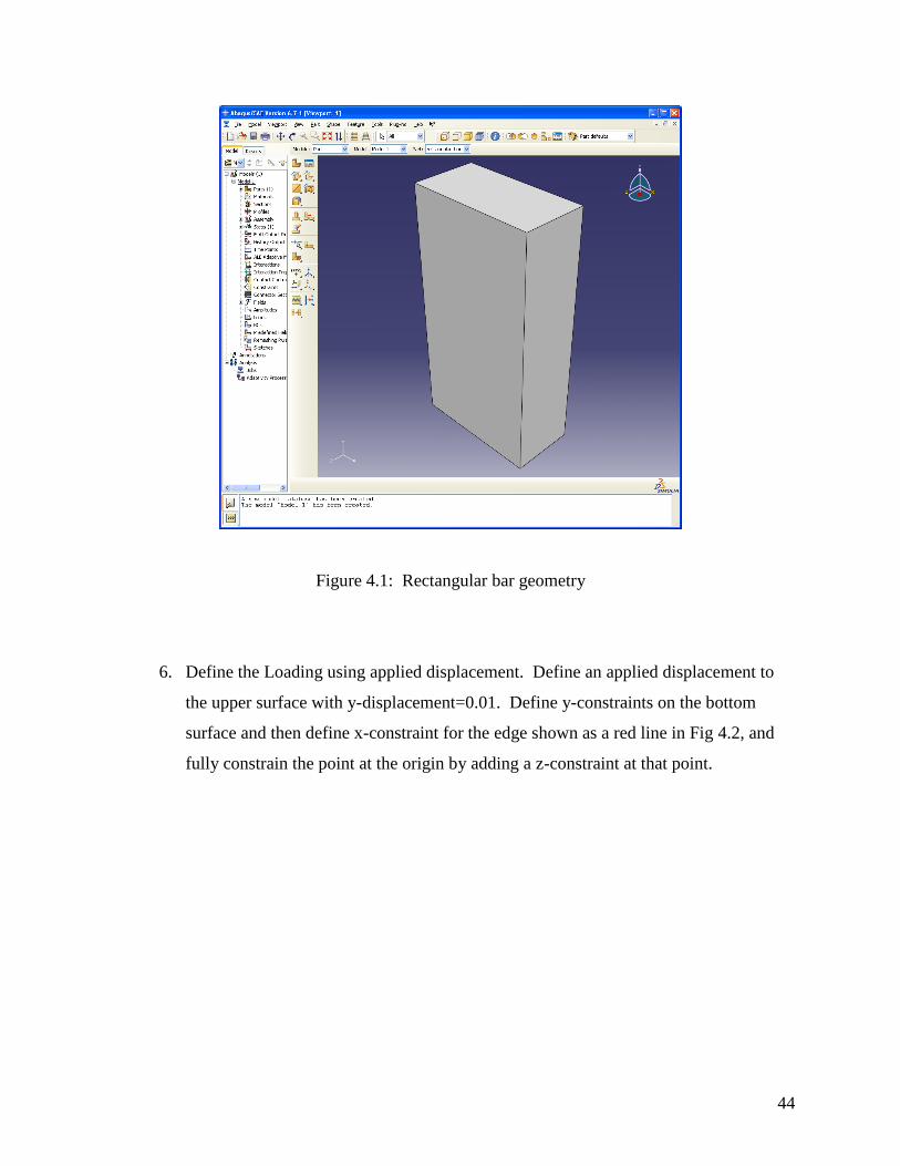
2. Create a new part named rectangular_bar by clicking the icon in the Part

Module, specifying the name and setting approximate size to 10. Click Continue …

to display the Sketch window. Create a rectangle starting at 0,0 with dimensions

x=0.5 and y=1.0. Click the red X at the bottom and click Done and specify 0.25 for

the depth. A rectangular bar will be created (Fig 4.1).

3. Define an elastic material with properties: E=10,000 and nu=0.3. Define the section

and assign the material to the section and attach to the geometry.

4. Create the Assembly, the mesh can be indepenedent.

5. Create the Step as a Static,General analysis load step.

44

Figure 4.1: Rectangular bar geometry

6. Define the Loading using applied displacement. Define an applied displacement to

the upper surface with y-displacement=0.01. Define y-constraints on the bottom

surface and then define x-constraint for the edge shown as a red line in Fig 4.2, and

fully constrain the point at the origin by adding a z-constraint at that point.

45

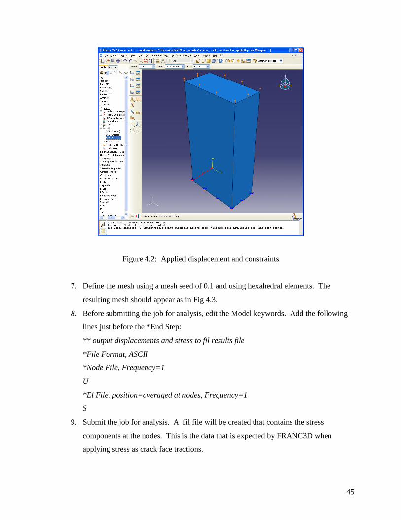
Figure 4.2: Applied displacement and constraints

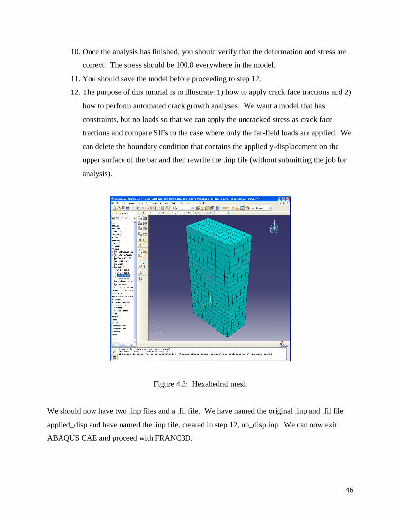
7. Define the mesh using a mesh seed of 0.1 and using hexahedral elements. The

resulting mesh should appear as in Fig 4.3.

8. Before submitting the job for analysis, edit the Model keywords. Add the following

lines just before the *End Step:

** output displacements and stress to fil results file

*File Format, ASCII

*Node File, Frequency=1

U

*El File, position=averaged at nodes, Frequency=1

S

9. Submit the job for analysis. A .fil file will be created that contains the stress

components at the nodes. This is the data that is expected by FRANC3D when

applying stress as crack face tractions.

46

10. Once the analysis has finished, you should verify that the deformation and stress are

correct. The stress should be 100.0 everywhere in the model.

11. You should save the model before proceeding to step 12.

12. The purpose of this tutorial is to illustrate: 1) how to apply crack face tractions and 2)

how to perform automated crack growth analyses. We want a model that has

constraints, but no loads so that we can apply the uncracked stress as crack face

tractions and compare SIFs to the case where only the far-field loads are applied. We

can delete the boundary condition that contains the applied y-displacement on the

upper surface of the bar and then rewrite the .inp file (without submitting the job for

analysis).

Figure 4.3: Hexahedral mesh

We should now have two .inp files and a .fil file. We have named the original .inp and .fil file

applied_disp and have named the .inp file, created in step 12, no_disp.inp. We can now exit

ABAQUS CAE and proceed with FRANC3D.

47

4.2 Step 2: Crack insertion with FRANC3D

The next step is to read the model into FRANC3D and insert a crack.

1. Copy the .inp files from the ABAQUS working directory to the FRANC3D working

directory – if they are different.

2. Start FRANC3D.

3. Select File and Open. In the Open Model File window, choose the ABAQUS FILES

(*.inp) file filter and applied_disp.inp file and Click OK.

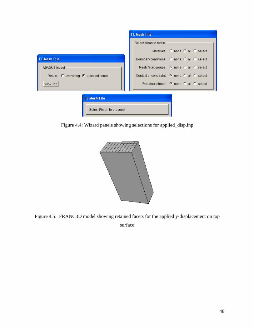
4. Follow the wizard through the panels shown in Fig 4.4. We choose selected items

and then choose all materials, all boundary conditions, and no mesh facets. The

resulting FRANC3D model is shown in Fig 4.5.

5. Insert the crack into the model by selecting Cracks and New Flaw Wizard. In the

Flaw Insertion window select Crack (zero volume flaw) and click Next. In the

following window, select the top-left crack type, the ellipse.

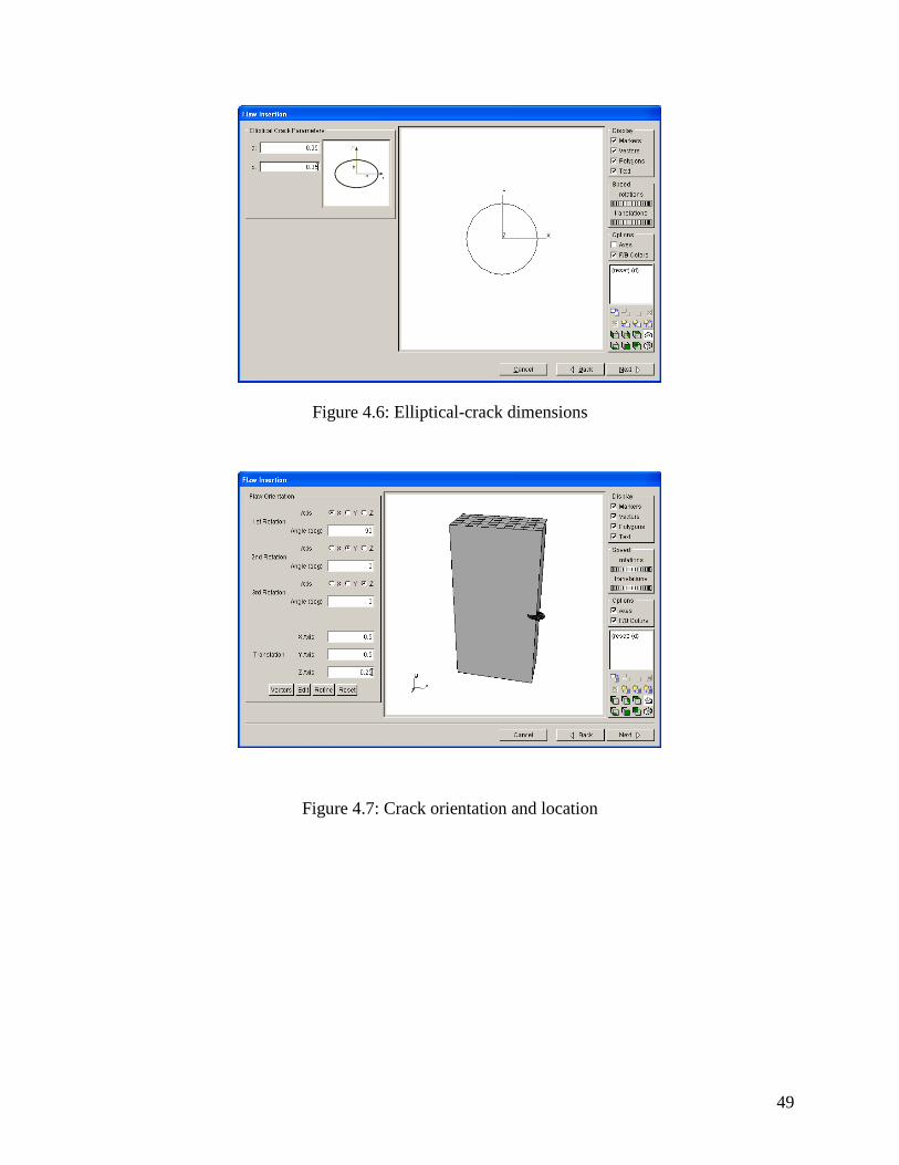
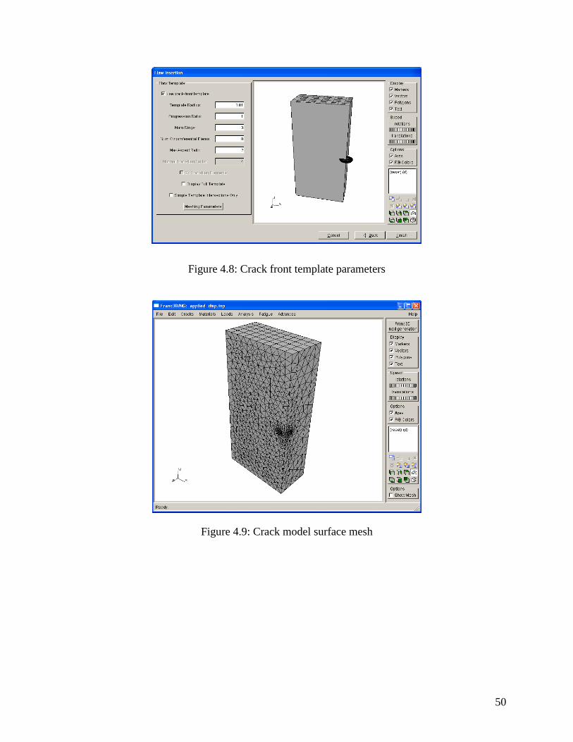
6. For the remaining wizard windows, follow the panels in Figs. 4.6 – 4.8, which show

the crack shape, location, orientation and template parameters used for this crack.

The meshed crack model is shown in Fig 4.9.

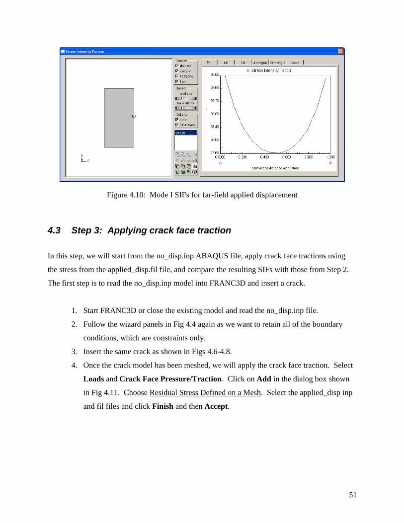
7. Perform a static crack analysis on this model to compute the SIFs for far-field

loading. Analyze the model using ABAQUS. The elements should be second order.

There is no global model to connect. All boundary conditions should be transferred.

If the ABAQUS analysis fails to run to completion, examine the .dat and .msg files

along with the FRANC3D terminal window for messages. Once the analysis finishes,

compute the SIFs; they should be as in Fig 4.10.

48

Figure 4.4: Wizard panels showing selections for applied_disp.inp

Figure 4.5: FRANC3D model showing retained facets for the applied y-displacement on top

surface

49

Figure 4.6: Elliptical-crack dimensions

Figure 4.7: Crack orientation and location

50

Figure 4.8: Crack front template parameters

Figure 4.9: Crack model surface mesh

51

Figure 4.10: Mode I SIFs for far-field applied displacement

4.3 Step 3: Applying crack face traction

In this step, we will start from the no_disp.inp ABAQUS file, apply crack face tractions using

the stress from the applied_disp.fil file, and compare the resulting SIFs with those from Step 2.

The first step is to read the no_disp.inp model into FRANC3D and insert a crack.

1. Start FRANC3D or close the existing model and read the no_disp.inp file.

2. Follow the wizard panels in Fig 4.4 again as we want to retain all of the boundary

conditions, which are constraints only.

3. Insert the same crack as shown in Figs 4.6-4.8.

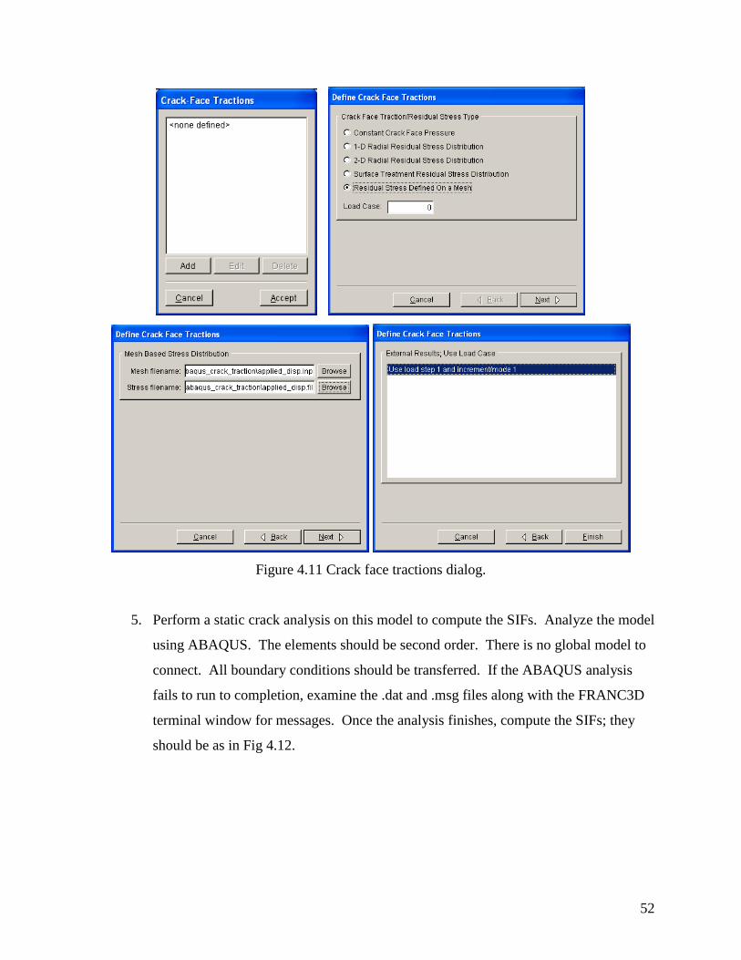
4. Once the crack model has been meshed, we will apply the crack face traction. Select

Loads and Crack Face Pressure/Traction. Click on Add in the dialog box shown

in Fig 4.11. Choose Residual Stress Defined on a Mesh. Select the applied_disp inp

and fil files and click Finish and then Accept.

52

Figure 4.11 Crack face tractions dialog.

5. Perform a static crack analysis on this model to compute the SIFs. Analyze the model

using ABAQUS. The elements should be second order. There is no global model to

connect. All boundary conditions should be transferred. If the ABAQUS analysis

fails to run to completion, examine the .dat and .msg files along with the FRANC3D

terminal window for messages. Once the analysis finishes, compute the SIFs; they

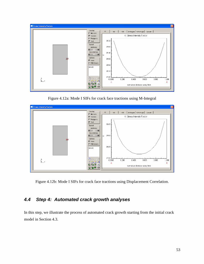
should be as in Fig 4.12.

53

Figure 4.12a: Mode I SIFs for crack face tractions using M-Integral

Figure 4.12b: Mode I SIFs for crack face tractions using Displacement Correlation.

4.4 Step 4: Automated crack growth analyses

In this step, we illustrate the process of automated crack growth starting from the initial crack

model in Section 4.3.

54

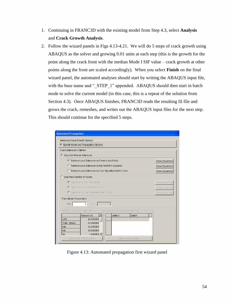
1. Continuing in FRANC3D with the existing model from Step 4.3, select Analysis

and Crack Growth Analysis.

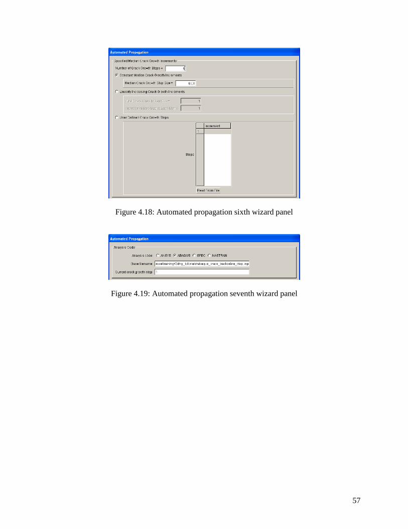
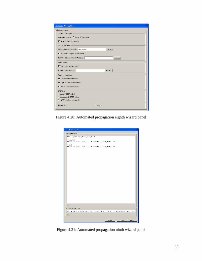
2. Follow the wizard panels in Figs 4.13-4.21. We will do 5 steps of crack growth using

ABAQUS as the solver and growing 0.01 units at each step (this is the growth for the

point along the crack front with the median Mode I SIF value – crack growth at other

points along the front are scaled accordingly). When you select Finish on the final

wizard panel, the automated analyses should start by writing the ABAQUS input file,

with the base name and “_STEP_1” appended. ABAQUS should then start in batch

mode to solve the current model (in this case, this is a repeat of the solution from

Section 4.3). Once ABAQUS finishes, FRANC3D reads the resulting fil file and

grows the crack, remeshes, and writes out the ABAQUS input files for the next step.

This should continue for the specified 5 steps.

Figure 4.13: Automated propagation first wizard panel

55

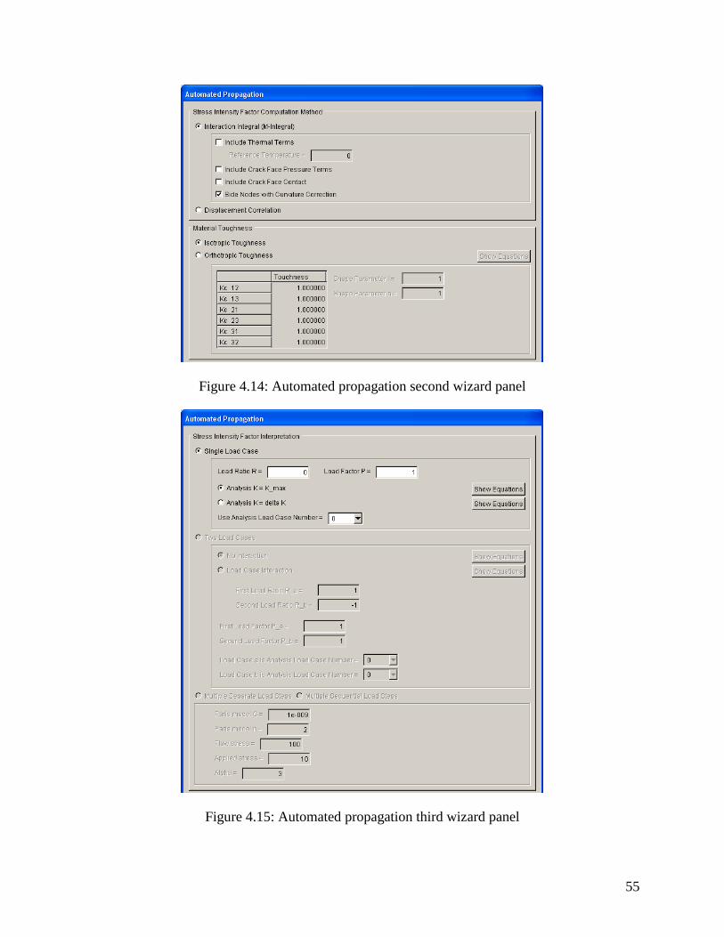
Figure 4.14: Automated propagation second wizard panel

Figure 4.15: Automated propagation third wizard panel

56

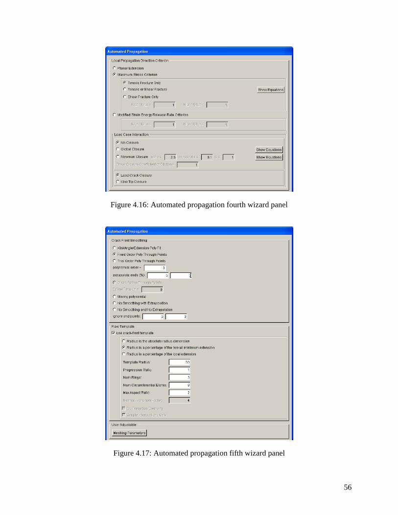
Figure 4.16: Automated propagation fourth wizard panel

Figure 4.17: Automated propagation fifth wizard panel

57

Figure 4.18: Automated propagation sixth wizard panel

Figure 4.19: Automated propagation seventh wizard panel

58

Figure 4.20: Automated propagation eighth wizard panel

Figure 4.21: Automated propagation ninth wizard panel

59

Once the 5 steps of automated crack growth are complete, you can read in the model and results

for any of the steps and compute SIFs. The SIF history can be extracted by computing and

exporting SIFs for each of the steps.

This is the end of the tutorial!