frank j. fabozzi edhec business school - weebly

Effects of Spot Market Short-Sale Constraints on Index Futures Trading*

Frank J. Fabozzi

EDHEC Business School

Ahmet K. Karagozoglu

Hofstra University

Na Wang

Hofstra University

March 2016

* We are grateful to Burton Hollifield (the Editor), an anonymous referee, George Papaioannou, Chris Stivers, Teng

Yuan Cheng and the seminar participants at the 2013 FMA meeting and the 2nd International Conference on Futures

and Derivative Markets for helpful comments and suggestions, and Xia Zhang and Lingchao Zuo for research

assistance. Frank J. Fabozzi is at EDHEC Business School, France, +33(0)493189966; [email protected].

Ahmet K. Karagozoglu is at Frank G. Zarb School of Business, Hofstra University, Hempstead NY 11549; (516)

463-5701; [email protected]. Na Wang is at Frank G. Zarb School of Business, Hofstra University, Hempstead

NY 11549; (516) 463-5498; [email protected].

mailto:[email protected]



1

Effects of Spot Market Short-Sale Constraints on Index Futures Trading

Abstract

We analyze the effects of spot market short-sale constraints on derivatives trading using a unique

Chinese stock market futures trading database. Due to short-sale constraints, investors’

pessimistic views on the underlying index can be expressed solely through short futures positions,

while investors’ optimistic views are dispersed through their spot and futures trading. We

hypothesize that trading of pessimistic investors (with net short futures positions) contains more

information than that of optimistic investors. We document the negative volatility-volume

relation is associated with pessimistic investors’ trading, which attenuates with less restricted

spot market short-sale rules. Large pessimistic investors’ net demand can predict future returns,

but not the case for optimistic investors.

Key Words: short-sale constraints, volatility-volume relation, pessimistic and optimistic large

investors, index futures

JEL Classification: G11, G13, C53

2

1. Introduction

Academics, practitioners, and regulators have long debated and studied the effects of

short-sale constraints on stock prices as well as the orderly functioning of equity markets.

Theoretical work can be traced back to Miller (1977) and Harrison and Kreps (1978) who show

that in the presence of short-sale constraints, asset prices tend to reflect the optimistic views of

the investors and prices may exceed the fundamental value of those assets. Since then, several

studies have highlighted the joint effects of the short-sale constraints and heterogeneous beliefs

in driving asset price bubbles and crashes (see, for example, Scheinkman and Xiong, 2003; Hong

and Stein, 2003). On the empirical side, numerous studies found consistent evidence that short-

sale constraints cause stock overvaluation, and the overvaluation is more dramatic among stocks

that are more difficult to arbitrage (see, for example, Lamont and Thaler, 2003; Chang et al.,

2007; Xiong and Yu, 2011; Stambaugh et al., 2012).

Alternatively, in the absence of restrictions, short sales promote market efficiency. For

example, Bris et al. (2007) analyze cross-sectional and time-series data from 46 equity markets

around the world and find evidence that prices incorporate negative information faster in

countries where short sales are allowed and practiced. Boehmer et al. (2008) study order-based

short sales and find that large short-sale orders are the most informative, and large informed

traders buy and sell within a relatively small range of prices around the fair value of an asset,

thus decreasing price volatility.

Although the literature on the effects of short-sale constraints in equity markets is

extensive, little is known about how the short-sale constraints in the spot market affect trading in

derivatives markets. Recently, the 2008 short-sale ban provided an opportunity for academics to

examine potential impact of spot market short-sale restrictions on a specific derivatives market

3

(e.g., options on individual financial stocks). 1 Battalio and Schultz (2011) investigate the

liquidity of options on the stocks subject to this short-sale ban. In addition to finding an increase

in options’ spreads, they highlight the increasing importance of considering the effects of spot

short-sale restrictions on related derivatives markets.

Figlewski and Webb (1993) contend that options alleviate stock market short-sale

restrictions due to the fact that synthetic short positions can be created using options contracts.

Furthermore, Blau and Wade (2013) show that trading of pessimistic investors shifts towards the

options market from underlying stocks when short-selling of those stocks becomes more

expensive. Following these two studies, we postulate that, due to short-sale constraints, investors

who cannot express their pessimistic views in the spot market through short selling the

underlying stocks can act on those views solely through holding net short positions in the

corresponding futures market.2 In contrast, investors with optimistic views of the spot market

may dilute the value of their information by holding long positions in either (or both) spot and

futures markets. Hence, net short futures positions taken by traders with pessimistic views are

expected to be relatively more informative than the net long futures positions taken by traders

with optimistic views.

Our paper explores, for the first time, the effects of spot market short-sale constraints on

futures market, specifically on the trading of stock index futures contracts. For this purpose, our

empirical methodology utilizes the volatility-volume relation and the return predictability of

investors with different spot market sentiment. Daigler and Wiley (1999) argue that the

1 The Securities and Exchange Commission (SEC) Rule 204T banned the short sales of certain financial stocks

between September 19 and October 8, 2008.

2 This is true as long as there are no options contracts or shortable exchange-traded funds (ETF) contracts available

on the underlying equities, which is the case for our empirical analysis.

4

volatility-volume relation varies with the amount of information investors possess. While

informed investors trade around the intrinsic value of assets and their trades are expected to

reduce the price volatility, uninformed or less informed traders may exaggerate price changes

and increase volatility. Therefore based on our hypothesis, we expect that trading by investors,

especially the ones holding large positions, with pessimistic views of the spot market is more

likely to be negatively correlated with futures volatility than trading by those with optimistic

views. In addition, the positions of the pessimistic investors are expected to predict future returns

better than those of optimistic investors.

We test our hypotheses using the daily trading data for the CSI 300 Index futures traded

at the China Financial Futures Exchange (CFFEX). China is ideal for testing our hypotheses for

the following reasons. First, short selling in the Chinese stock markets has explicit restrictions,

with a limited number of stocks under a pilot program allowed for short-selling.3 In particular,

since the introduction of the CSI 300 Index futures in 2010, the short-sale pilot program has been

expanded twice, offering us an opportunity to investigate the effects of variations in the degree of

short-sale restrictions. Second, the CFFEX has disclosed the daily trading volume and positions

of the largest 20 trading firms, which we refer to later as large investors.4 The detailed daily

disclosure data allows us to identify the pessimistic versus optimistic views of the large investors

and track the different effects of their trading. The orderly relaxation of short-sale restrictions as

well as the existence of only a single type of derivatives on the stock market provide us cleaner

tests compared to the 2008 short-sale ban. Grundy et al. (2012) indicate that 2008 short-sale ban

is “implemented as a response to unusual market conditions.” Battalio and Schultz (2011)

3 See the detailed discussion in Section 2 and 3.

4 Anecdotally, the daily disclosure is intended to discourage potential excessive speculation in the CSI 300 Index

futures contracts by large investors, and only the largest 20 trading firms are disclosed.

5

highlight the extensive regulatory uncertainty throughout the entire duration of this

unprecedented event.5

Our findings are as follows. We show that the negative volatility-volume relation is

mostly associated with the trading by pessimistic investors, the group of the large investors

holding net short positions in the index futures contracts. In contrast, trading by large investors

with optimistic views exhibits no significant effect on futures volatility. After the expansion of

the short-sale pilot program (i.e., as short selling becomes less restricted), we find that the effects

of pessimistic investors’ trading weakens in terms of decreasing volatility.

By further analyzing the daily disclosure data of the large futures trading firms, we

document varying effects of different types of exchange membership on the volatility-volume

relation. The negative volatility-volume relation is more pronounced for the activity of

pessimistic trading members who can only transact for their own accounts. Activity of clearing

members, who can transact for both their own and client accounts, does not appear to be as

informative. This finding suggests that the activity of pessimistic trading members is relatively

more informative than those of the optimistic trading members as well as both the pessimistic

and optimistic clearing members.

Lastly, we provide further evidence on the informativeness of the pessimistic and

optimistic large investors’ trading activity by investigating the return predictability of their net

futures positions. We find that the net position of large pessimistic investors is able to correctly

5 Battalio and Schultz (2011) state that “the short sale ban, which was to take effect immediately, was announced in

the early morning hours of September 19 with no prior warning to market participants. Numerous officials of the

options exchanges, some of whom we cite, complained that the ban resulted in great uncertainty both about how the

ban was to be implemented and about possible additional regulation.”

6

predict future returns within a week, and this prediction is mainly significant for the pessimistic

trading members.

Our study contributes to the literature by providing new evidence for the effects of spot

market short-sale constraints on the trading behavior and asset prices in the derivatives markets.

For example, Battalio and Schultz (2011) and Grundy et al. (2012) focus on the effects of 2008

short-sale ban on the equity option markets in the US.6 McMillan and Philip (2012) study the

spot and futures cross-market efficiency implications of the short-selling constraints imposed in

nine countries during the financial crisis, and find that arbitrage is less effective during the ban

period. They focus on the pricing relationship between the spot equities and futures contracts on

those individual stocks. We take a different approach by looking at how the spot market short-

sale constraints affect the relative informativeness of the activity by pessimistic versus optimistic

futures traders. We provide the first evidence in the literature that the negative volatility-volume

relation in futures markets is mostly associated with the trading of pessimistic investors, and this

negative relation weakens as spot market short-selling gets less restricted.

Our study also sheds light on the literature of the informational efficiency of short sales.

On one hand, there are a good number of studies showing that constrained short sales are

detrimental for market efficiency. For example, Beber and Pagano (2013) find that short-sale

bans decrease stock liquidity and slow price discovery. Boehmer et al (2013) document large-cap

stocks subject to the ban suffered a severe degradation in market quality. Boulton and Braga-

6 Although analysis of Grundy et al. (2012) consider the single stock futures and ETFs in addition to options, these

potential alternative derivative markets have extremely low liquidity before and during the short-sale ban. In

addition, the authors conclude that “short-sale ban acts as an effective restriction on trading in options”. Therefore,

we believe that our extension of this line of inquiry is well warranted and our research makes significant

contribution to the literature in part because our results are not affected by various confounding forces.

7

Alves (2010) also find the restrictions negatively impact various measures of liquidity. On the

other hand, many studies, such as Jarrow (1980), Figlewski (1981), Diamond and Verrecchia

(1987), and Chen et al. (2002), present mixed results. For example, Diamond and Verrecchia

(1987) show that short-selling bans reduce the speed of price discovery, but the effect on the bid-

ask spread is ambiguous. Our study adds new evidence to the literature of information efficiency

with a set of particularities for the Chinese equity markets, such as the gradual removal of short-

sale restrictions and the transparency in the identification of trading positions. We show that as

the short-sale restriction is lifted, the information advantage of traders with net short positions in

the futures market gradually weakens, indicating that part of the information contained in the

trading activities of pessimistic investors gets incorporated into the underlying markets.

Consistent with our conjecture, studies focusing on the effects of short-sale regulations on

Chinese stock markets, such as Chang et al. (2014), show that stock price efficiency increases

after the short-sale ban is lifted. The implication is that unrestricted short sales improve market

efficiency, and markets should favor unrestricted shorting rules.

The rest of the paper is organized as follows. Section 2 discusses the related literature and

testable hypotheses. Section 3 describes the data and institutional details, followed by a

description of the construction of our trading and position variables and volatility estimates in

Section 4. Section 5 presents our empirical analysis and findings. Section 6 concludes.

2. Related Literature and Testable Hypothesis

We investigate the effects of spot market short-sale constraints on the futures market

volatility-volume relation and the return predictability of trading by investors with different spot-

market sentiment. The volatility-volume relation has been studied within various theories and

models. The dispersion of beliefs and information models proposed by Harris and Raviv (1993)

8

and Shalen (1993) suggest that the volatility-volume relation depends on who is generating

volume and how much information they perceive. Informed traders buy and sell within a

relatively small range of prices around the fair value of the assets and hence their trades decrease

the price volatility. While uninformed (or less-informed) traders are likely to react to all changes

in volume and price as if they reflect information, hence they tend to exaggerate price

movements and result in greater price variability. The volatility-volume relation has also been

analyzed in complementary rather than competing theories and models. For example, the mixture

of distribution hypothesis (Clark, 1973; Harris, 1986; Tauchen and Pitts, 1983) assumes that the

number of information arrivals causes the joint distribution of volatility and volume. In this

paper, our goal is not to distinguish between the different theories driving this volatility-volume

relation; instead, we use the volatility-volume relation framework to identify the relative

informativeness of trading by futures markets participants with different spot market sentiment

and to investigate the effects of spot market short-sale constraints on futures markets.

To do so, we focus on the Chinese equity markets where the existence and changes of the

spot market short-sale restrictions provide a unique opportunity for our study. Short selling has

explicit and implicit constraints in the Chinese equity markets with approximately 2,000 stocks

listed for trading. Short-selling was completely banned prior to March 31, 2010. The China

Securities Regulatory Commission (CSRC) then initiated a pilot program allowing short-sale of

90 selected stocks by qualified investors. Stocks selected for the pilot program had to meet

certain criteria based on size, liquidity, and volatility.7 The requirements for qualified investors,

7 More specifically, a firm must have no fewer than 200 million tradable shares and a public float no less than RMB

800 million. The number of shareholders must be no fewer than 4,000. In any given day during the past three

months, the daily turnover must be no lower than 15% of index turnover, the daily trading value must be no lower

than RMB 50 million, its average return must not deviate more than 4% from the index return, and its return

9

differing across security and brokerage firms, place implicit constraints on short-selling in this

limited scale (see Chang et al., 2014). Furthermore, Stambaugh et al. (2012) argue that short-sale

impediments in stock markets exist implicitly due to institutional constraints, arbitrage risk,

behavioral biases of traders, and trading costs.

During our sample period, options contracts or domestic shortable exchange-traded funds

(ETFs) were not available for investors to trade in Chinese financial markets.8 Therefore, the

existence of only stock index futures eliminates the confounding effects of alternative derivatives

with differential liquidity, a concern in the studies focusing on the 2008 short-sale ban described

earlier.

As a result of the spot market short-sales restrictions, investors can only express their

pessimistic views of the stock market through taking short positions in the index futures market,

while optimistic views of investors can be dispersed between the spot and futures markets as

they hold long positions in either or both markets. Note that investors can hold a long position in

the spot markets through purchasing index mutual funds or ETFs, which make it relatively easier

holding the long positions than holding short positions in the spot markets. Therefore, we expect

that the trading of the pessimistic large investors in the index futures contract is relatively more

informative than that of the optimistic investors, producing a stronger negative effect on futures

return volatility. Therefore, the main hypothesis of our paper is:

volatility must be no higher than five times of the index volatility. Among all the companies eligible for short-selling,

the CSRC randomly selected 90 firms in the initial pilot program. Similar criteria was applied when the CSRC

expanded the pilot program in 2011 and 2013.

8 Although domestic ETFs existed during our sample period, there were no inverse ETFs which could be traded to

act on a pessimistic market view of the market, and short selling of domestic ETFs were not permitted.

10

HYPOTHESIS 1. Due to short-sale restrictions, trading of large investors with

pessimistic views of the spot market is more likely to be negatively correlated with return

volatility of the futures contracts than trading by those with optimistic views.

During our sample period, the short-sale pilot program has been expanded twice, on

December 5, 2011 and on January 31, 2013, increasing the number of stocks available for short-

selling. We are able to use the variations in the degree of short-sale restrictions as a natural

experiment to further test our hypothesis. We expect that the negative volatility-volume relation

of the pessimistic investors’ trading weakens as more stocks can be short-sold in spot market,

these investors can now act on their pessimistic views in both the futures and underlying spot

markets. However, due to the limited scale of the pilot program and the implicit short-sale

constraints described by Stambaugh et al. (2102), we do not expect this negative relation to

disappear. Hence, our second hypothesis is:

HYPOTHESIS 2. The negative volatility-volume relation of the pessimistic investors’

trading attenuates as short selling gets less restricted.

To further investigate the effects of spot market short-sales restrictions on the stock index

futures trading, we examine the return predictability of net positions of both the pessimistic and

optimistic large investors. Return predictability in the futures market has been widely explored in

the literature. For example, Wang and Yu (2004) analyze the daily price, volume, and open

interest data on 24 futures contracts traded in the United States. They find that in addition to

historical prices, lagged trading volume and open interest correlate significantly with future price

changes. Wang (2004) investigates the relation between trading volume and return predictability

in currency futures and finds that trading strategies are profitable when contrary to the position

11

changes of hedgers but consistent with those of speculators. We expect that trading by large

investors with pessimistic views of the underlying spot market who cannot act on their views in

spot market due to short-sale restrictions, would better predict returns in the futures prices.

Consequently, our third hypothesis is:

HYPOTHESIS 3. Due to the short-sale restrictions in the spot market, the pessimistic

large investors’ positions (net-demand) in futures market are more informative in

predicting future returns.

3. Data and Institutional Background

3.1 Data and Regulations in the Chinese Markets

The data used in our study are the CSI 300 Index futures contracts traded in the China

Financial Futures Exchange (CFFEX). The CSI 300 Index is a market capitalization weighted

index of 300 A-shares stocks listed in China’s two stock exchanges, the Shanghai Stock

Exchange and the Shenzhen Stock Exchange. The CFFEX was established in Shanghai on

September 8, 2006, and within two months it launched the CSI 300 Index futures mock trading

system, which was modified in 2007. Actual trading of the CSI 300 Index futures contract

formally started on April 16, 2010. CSI 300 Index futures contracts trade in monthly cycles:

current month, next month, and next two calendar quarters (a total of four contracts).

We obtained the top 20 large trader volume and position data for the CSI 300 Index

futures contracts from the CFFEX. At the end of each trading day, the exchange discloses on its

website the identities of firms whose trading volume, long positions, or short positions rank them

12

within the top 20 largest trading firms on that day, together with each firm’s actual volume, long

and short position values.9

The CFFEX uses a multi-tiered clearing system, comparable to those used by many

overseas markets, that divides exchange members into different tiers in accordance with their

tolerance to risk. Members in different tiers have different business scope which enables to

construct a multi-tiered risk control system to hedge risks efficiently and to improve the

exchange’s overall risk control capability. 10 The first tier of this system divides exchange

members into two categories: clearing members and non-clearing members. Non-clearing

members engage in proprietary trading and/or brokerage business but are not allowed to do the

clearing directly with the exchange. Exchange’s clearing membership group is further divided

into three member categories: trading-clearing, general-clearing and special-clearing. The

special-clearing members can only engage in clearing and settlement for non-clearing members.

The trading-clearing members are only eligible to trade and engage in clearing and settlement for

their own accounts while the general-clearing members are allowed engage in all three activities

for both their own accounts and for non-clearing members. We have obtained the exchange

membership directory containing the identities and classification of member firms and our

dataset of the daily top 20 largest trading firms consists of trading-clearing members and general-

clearing members.

In addition to the unique and detailed disclosure data, we also obtained the daily futures

settlement prices, trading volume and open interest data for all contract months from the CFFEX.

Our intraday data for the CSI 300 Index futures contract is collected from the Bloomberg

9 CFFEX only discloses for the top 20 largest trading firms ranked by their trading volume and positions, and such

detailed information is not disclosed for the rest of the trading firms.

10 This information is available from the CFFEX website: http://www.cffex.com.cn/en_new/gyjys_6434/jyjg/.

13

Professional terminal. For each trading day, we recorded the open, high, low, close prices as well

as the number of contracts traded for each 1-minute interval. Our sample period is from the

launch date of the CSI 300 Index futures, April 16, 2010 to November 15, 2013 for our intraday

and daily data.

Two weeks before the launch of the CSI 300 Index futures, on March 31, 2010, the China

Securities Regulatory Commission’s (CSRC) initiated a pilot program for short-selling of 90

stocks (50 stocks listed in the Shanghai Stock Exchange and 40 stocks in the Shenzhen Stock

Exchange). All of the 90 stocks were members of the CSI 300 Index on that day. During our

sample period, the short-sale pilot program has been expanded twice, on December 5, 2011 and

on January 31, 2013. Table I presents the details of the expansion of the short-sale pilot program.

On December 5, 2011, the CSRC increased the number of stock allowed for short-selling to 278,

of which 260 stocks were members of the CSI 300 Index on that day. On January 31, 2013, total

number of stocks allowed for short-selling under the pilot program was increased to 500 and this

list contained all of the 300 members of the CSI Stock Index on that day. We have obtained the

names and index weights of all stocks in the CSI 300 Index on each of the above dates from the

Bloomberg Professional terminal and calculated the proportion, based on market capitalization,

of the CSI 300 Index stocks which were allowed to be short-sold under the pilot program. The

stocks in the short-sale pilot program counted for 63.8% of the value of CSI 300 when the index

futures trading started on April 16, 2010; this proportion increased to 96% and to 100% of the

value of the index on December 5, 2011 and on January 31, 2013, respectively. Expansion of the

pilot short-sale program provides us a unique setup in testing of our hypothesis as short-sale

restrictions are explicitly relaxed for the stock in the CSI 300 Index.11

11 Note that our main variables of interest, the pessimistic and optimistic volume, are the trading volumes of the

index futures contracts, variables that are not derived specifically from stocks in the pilot program. Our empirical

14

3.2 Related Foreign Financial Products

Although short sales in the Chinese markets are restricted, foreign ETFs on the China

region (e.g., FXI, MCHI, and CHIX) existed during our sample period, and large institutional

investors could have resources to short them in foreign markets. Institutional investors could

also achieve short positions through trading inverse and leveraged ETFs (e.g., YANG, YXI,

YINN, and XPP) or shorting Chinese American depositary receipts (ADRs) traded in foreign

markets. However, we believe there are at least two reasons why these foreign products may

not affect our main findings regarding the information advantage of large traders holding net

short positions in the futures market.

First, only a small number of Chinese institutions can invest in foreign financial

markets, and such investments are highly regulated. During our sample period, there were a

total of 58 institutions that fall into what the Chinese regulators classify as “Qualified Domestic

Institutional Investors”, who are allowed to invest in foreign securities. Among these qualified

institutions, only seven of them have sub-companies that trade the CSI 300 Index futures

contract. Furthermore, three of the seven sub-companies trade futures occasionally (e.g.,

appearing in the top-20 lists less than one third of the trading days). Comparing to the total

number of 145 trading firms appearing in the top-20 list, the aggregate effect of shorting foreign

financial products on the CSI 300 Index futures trading tends to be limited.

analyses of the index futures trading are more related to the relative restrictive level of the short-sale regulations

(e.g., expanding the short-sale list from 90 to 260 stocks in the CSI 300 Index), and less sensitive to which stocks

were selected for the short-sale pilot program. So we believe the stock selection criteria for the pilot program should

not lead to endogeneity issues in our empirical design, and neither should it have a major impact on our empirical

findings.

.

15

Second, the existence of alternative foreign financial products could lead to no

significant effect of the net short positions in the stock index futures contract because

pessimistic investors could also express their negative opinions by shorting foreign products in

which the underlying assets are from the Chinese equity markets. But even with the potential

information dilution resulting from large investors taking short positions in foreign markets, we

are still able to document a significant negative effect of the pessimistic opinions on futures

volatility (see Section 5). Therefore, the relative information advantage of pessimistic versus

optimistic large investors in the futures market could not be (totally) eliminated by the

information dilution caused by trading in foreign financial products. The existence of the

related foreign financial products and trading of those products would not affect our main

conclusions.

4. Variable Construction

4.1 Pessimistic versus Optimistic Volume and Position Variables

We first focus on trading volume of the top 20 largest traders, and classify them as

pessimistic versus optimistic traders based on their net positions.12 The non-top 20 investors are

classified as small traders:

Optimist-Volume: is the sum of trading volumes of the top 20 largest investors whose long

futures position is greater than (or equal to) their short position—investors with net long

position—at the end of previous trading day.

12 In our empirical analysis we use the natural log of volume and position variables (measured in number of

contracts).

16

Pessimist-Volume: is the sum of trading volumes of the top 20 largest investors whose long

futures position is smaller than their short position—investors with net short position—at the

end of previous trading day.13

Small-Volume: is the trading volume by non-top 20 investors, which is calculated as the total

futures trading volume minus the sum of Optimist-Volume and Pessimist-Volume on the same

trading day.

Next, we categorize the net demand of the top 20 largest investors based on the difference

in their long and short futures positions at the end of a trading day:

Optimist-Net-Demand: total long positions minus total short positions of the top 20 largest

investors whose long futures position is greater than (or equal to) their short position, i.e.

traders holding net long position at the end of a trading day. In our empirical analysis, we use

the scaled net-demand value, dividing the Optimist-Net-Demand by the total open interest at

the end of each trading day.

Pessimist-Net-Demand: total long positions minus total short positions of the top 20 largest

investors whose long futures position is less than their short position, i.e. traders holding net

short position at the end of a trading day. Again, we scale the Pessimist-Net-Demand by the

total open interest at the end of each trading day in our analysis.

We further partition our pessimistic and optimistic volume and net-demand variables for

the top 20 largest investors based on their exchange member classification. Since our disclosure

13 We use the sum of volumes to capture the aggregate information content of pessimists versus optimists. Sum of

the trading volumes have been used in the literature to study the information effects of the different types of traders

on the volatility-volume relation (e.g., Chen and Diagler 2000 and Daigler and Wiley 1999). In Section 5.3, we also

discuss results based on alternative volume measures to address the potential bias caused by the actions of one or

two large trading firms.

17

data is for the top 20 largest members, it is not surprising that we do not observe non-clearing

members or special clearing members who, by classification, are expected to be smaller in

general.

In our analysis, Trading Members refer to those firms classified by the CFFEX as

trading-clearing members, because they are only eligible to trade and engage in clearing and

settlement for their own accounts. Similarly, we refer to the general-clearing members as

Clearing Members, because this group of firms can trade, clear and settle futures contracts for

both their own accounts and for non-clearing members. Since our disclosure data do not break

down the volume and positions of the clearing members for own-account vs. customer accounts,

we expect that the trading members’ activities to be more informative, due to the fact that a

clearing member and its various clients may have opposing views and motivations leading to

noisier volume and position values.

Then we classify the volume and position variables for pessimistic large investors as

Trading Member Pessimist-Volume, Clearing Member Pessimist-Volume, Trading Member

Pessimist-Net-Demand and Clearing Member Pessimist-Net-Demand. For example, Trading

Member Pessimist-Volume is the sum of trading volumes of the top 20 largest firms classified as

Trading Members and whose long futures position is less than their short position—investors

with net short position—at the end of previous trading day. The corresponding volume and net-

demand variables for optimistic large trading firms are classified similarly in our analysis.

Finally, we define two time serial dummy variables to capture the changes in the short-

sale restrictions during our data period:

D2011: an indicator of the time period before or after December 5, 2011, which takes the

value of 1 if trading day is on or after December 5, 2011 and value zero otherwise.

18

D2013: an indicator of the time period before or after January 31, 2013, which takes the

value of 1 if trading day is on or after January 31, 2013 and value of zero otherwise.

We are particularly interested in the coefficients of the interaction terms of the short-sale

restrictions dummies and volume variables. The first expansion of the pilot program in 2011

results in a change in spot short-sale restrictions on the CSI 300 Index by 32.2% (= 96.0% -

63.8%), which is larger than that caused by the second expansion (4% = 100% - 96%). Therefore,

we expect that the impact of changes in spot short-sale restrictions on the CSI 300 Index futures

trading to be larger and more prominent in 2011 than that in 2013 (regarding the coefficients of

interaction variables for D2013).

4.2 Volatility Estimation

We estimate the unconditional return volatility based on intraday 1-minute intervals using

four different measures to provide robust empirical results. First, we calculate the absolute value

of returns for each minute in a trading day, which is a simple measure of unconditional volatility.

Forsberg and Ghysels (2007) show that this volatility measure predicts the quadratic returns very

well.

Second, we use a reduced form of the volatility measure developed by Garman and Klass

(1980). In our analysis, this measure is based on intra-minute price ranges:

2 2 1/2

, , , , ,{0.5 [ln( ) ln( )] [2ln(2) 1][ln( ) ln( )] }m t m t m t m t m tVolatility High Low Open Close (1)

where Highm,t, Lowm,t, Openm,t, and Closem,t are the high, low, open, and closing prices of the CSI

300 Index futures at each minute m of day t, respectively. Garman and Klass (1980) compare the

19

relative efficiency of several volatility measures, and conclude that their proposed measure

provides the highest efficiency.14

Next, we utilize the unconditional volatility measure proposed by Rogers and Satchell

(1991). One of the assumptions of range-based volatility estimations, such as the Garman-Klass

(1980) measure, is that prices follow random walk with zero drift. Rogers and Satchell (1991)

suggest that intraday prices may contain a drift component and propose a volatility estimate

model which is drift-independent:

, , , , ,

1/2

, , , ,

{[ln( ) ln( )][ln( ) ln( )]

[ln( ) ln( )][ln( ) ln( )]}

m t m t m t m t m t

m t m t m t m t

Volatility High Open High Close

L Open L Close

(2)

Finally, we include the simple range-based volatility estimate of Parkinson (1980):

2 1/2

, ,t ,{[ln( ) ln( )] / [4ln(2)]}m t m m tVolatility High Low (3)

After calculating the above volatility measures for each 1-minute time interval, we use

the median of 1-minute volatilities for each day as our measure of volatility under each method.15

Table II presents the summary statistics for the futures returns, volatility estimates, and

the pessimistic and optimistic volume and net-demand variables. Over the entire sample period,

the average of future returns is negative, with the standard deviation of 1.45%.16 The disclosed

trading volume and net demand of large pessimistic investors have similar magnitudes as those

of the optimistic investors in the CSI 300 Index futures contract. Figure 1 shows that over our

sample period the Chinese stock market declined as measured by the spot level of the CSI 300

14 The Garman-Klass volatility measure has been widely used in various studies of futures return volatility; for

example, see Daigler and Wiley (1999) and Wang (2002).

15 Using the average of 1-minute volatility for each day yields similar results.

16 We test whether futures returns follow a unit root process using Dickey and Fuller (1979), and we reject the null

hypothesis at 99% confidence level.

20

Index, while the spot trading volume did not have a consistent upward or downward trend.

Clearing Members in general exhibit larger trading volume than Trading Members, which is also

true when we separate the volumes by pessimists and optimists. A similar pattern is observed

regarding the net demand of the different member types. We also see in Table II that the mean

intraday 1-minute based volatility estimates derived from the four measures have similar

magnitudes. The Garman-Klass measure has the largest mean of 0.079% and the largest variation

of 0.025%.

5. Empirical Analysis

5.1 Short-Sale Restrictions, Investor Trading and Index Futures Volatility

Using the four different daily intraday 1-minute based measures of futures return

volatility—Absolute Return, Garman-Klass, Rogers-Satchell, and Parkinson—we investigate our

first hypothesis of the effects of short-sale restrictions on volatility-volume relation of investors

with pessimistic versus optimistic views (Optimist-Volume and Pessimist-Volume):

1 2 3

4 1 5 2 6

7

- - -

+

t t t t

t t

t t

t

Volatility Pessimist Volume Optimist Volume Small Volume

Volati Open Interest

Total Trading Volu

lity Volatility

me

(4)

where Volatilityt represents either Absolute-Return, Garman-Klass, Rogers-Satchell, or

Parkinson estimates, and Small-Volumet is defined in Section 4.1. Following Bessembinder and

Seguin (1992; 1993) and Chan and Fong (2000), our model includes Open Interestt and change

in the daily total trading volume ( Total Trading Volumet), which according to these studies, are

potentially correlated with the trading activities of informed traders. Additionally, 1- and 2-day

21

lagged volatilities (Volatilityt-1 and Volatilityt-2) are included to control for the persistence in

volatility.17

For all the regressions of the daily intraday 1-minute based volatility measures, we use

ordinary least squares (OLS) estimations with t-statistics calculated from heteroscedasticity and

autocorrelation consistent (HAC) Newey-West (1987) standard errors with optimal lag

specification based on the Akaike information criterion (AIC).

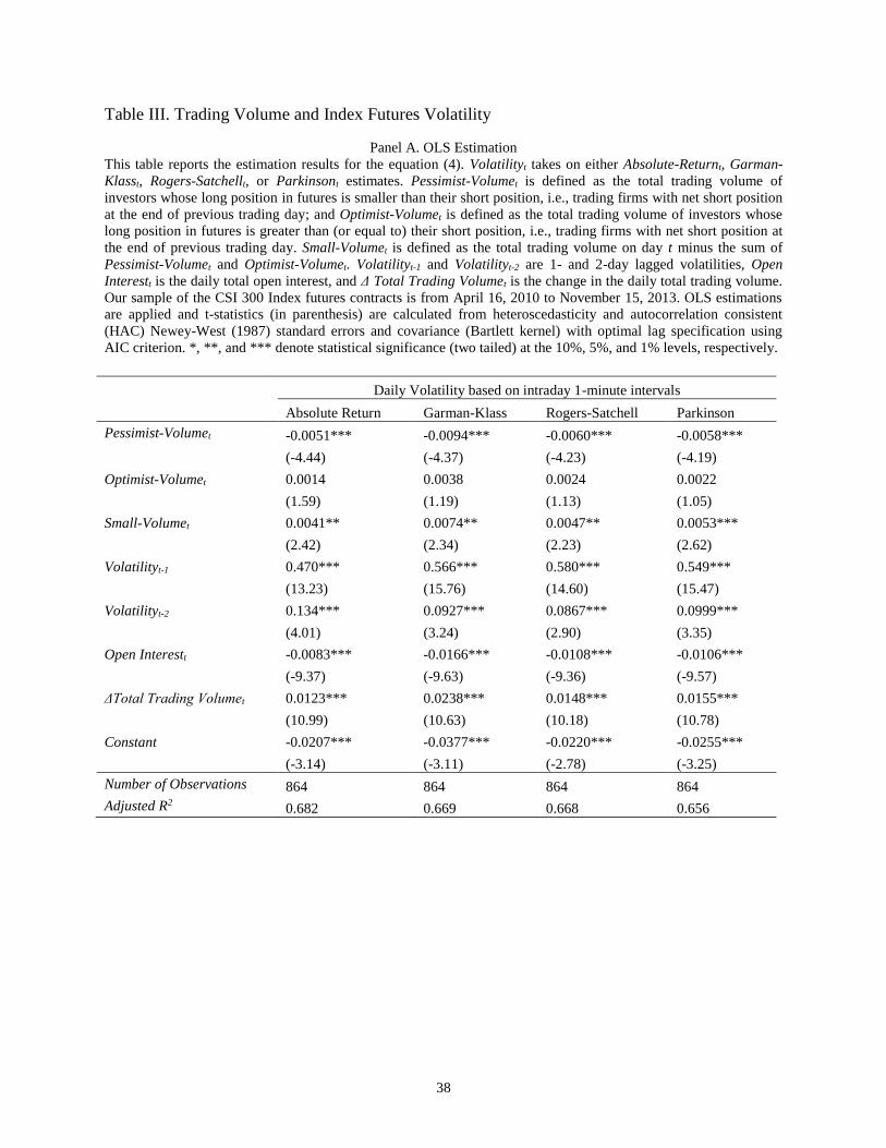
Our estimation results are presented in Panel A of Table III.18 When we use Absolute

Return as the estimate of unconditional volatility in Column 1, we find that trading by large

investors with pessimistic views of the underlying spot market (Pessimist-Volume) is negatively

correlated with the futures return volatility at the 1% significance level, while the trading by

large investors with optimistic views (Optimist-Volume) is not significantly correlated with

volatility. Column 2 shows that when we use the Garman-Klass volatility estimate, trading by

large investors with pessimistic views of the spot market (Pessimist-Volume) decreases futures

return volatility significantly, while the trading by large investors with optimistic views

(Optimist-Volume) does not have a significant effect on volatility. Note that the economic

significance of the negative effect of Pessimist-Volume on Volatility is large. For example, a one

standard deviation increase in Pessimist-Volume could decrease the volatility Garman-Klass by

25.9% (= 0.0094 × 0.688/0.025) of its standard deviation. The results using volatility measures

of Rogers-Satchell (Column 3) and Parkinson (Column 4) are very similar to those using the

Absolute Return and Garman-Klass estimates. We document both a statistical and an

17 Since we detect persistence in daily intraday 1-minute based volatility measures, models include all the significant

lags (i.e., the first two lagged volatilities).

18 Panel B of Table III presents results using Generalized Linear Models estimation which we refer to in our

discussion of robustness in Section 5.3.

22

economically significant negative volatility-volume relation of the Pessimist-Volume, but no

significant relation with the Optimist-Volume.

These results support with our first hypothesis that due to short-sale restrictions, trading

by pessimistic large investors is relatively more informative than that of the optimistic large

investors. The results hold after controlling for the level of open interest, changes in market-wide

trading and persistence in volatility.

Moreover, we find that the trading by small investors is significantly positively correlated

to the return volatility of the CSI 300 index futures, a finding which is uniform across all

measures of volatility. This is consistent with the argument in Daigler and Wiley (1999) that

small investors are more likely to trade as noise traders, and their trading exacerbates price

movements and is associated with higher volatility.

5.2 Impact of Changes in Short-Sale Restrictions on Trading and Index Futures Volatility

We further investigate the impact of spot short-sale restrictions on the relationship

between index futures volatility and trading volume of pessimistic and optimistic large investors.

We use the variations of the degree of short-sale restrictions and incorporate two time-serial

dummy variables following the regulation changes of the short-sale rules. We estimate the

following model:

2

1 2 1

2 2

1 1

3 4 1 5 2 6

7

- -

-

-

-

t t t j j jt

j j t jt j j t jt

t t t t

Volatility Pessimist Volume Optimist Volume Dummy

Pessimist Volume Dumm

Open Interest

y Optimist Volume Dummy

Small Volume Volatility Volatility

ttTotal Trading Volume

(5)

where Dummyjt variables are D2011t and D2013t as defined in Section 4.1, and the rest of the

variables are defined similarly as in equation (4).

23

Our main variable of interest is the interaction term of Pessimist-Volume and D2011.

Since short-sale restrictions have been alleviated on a larger scale after December 5, 2011, we

expect the negative volatility-volume relation to be weaker, which is equivalent to a positive

coefficient of Pessimist-Volume×D2011. Panel A of Table IV reports the results incorporating

the short-sale restrictions dummy variables.

Consistent with our Hypothesis 2, we find a significant positive coefficient for Pessimist-

Volume×D2011, regardless of the volatility measures we use. The economic significance is also

large. For example, when volatility is measured by Garman-Klass in Column 2, the volatility-

volume relation of Pessimistic-Volume drops to -0.0057 (= -0.0135 + 0.0078) after December 5,

2011, a decline about 42% (= 0.0057/0.0135) of its original effect. This supports our hypothesis

that the negative volatility-volume relation of the pessimistic investors weakens with less

restricted short-sale rules. However, the interaction term of Pessimist-Volume×D2013 does not

have a significant coefficient. This can be attributed to the fact that additional 4% short-sale

coverage in the CSI 300 Index after January 31, 2013 does not make significant difference

comparing to the previous 96% short-sale coverage.

Again, there is no significant relation between the Volatility and Optimist-Volume, and

the interaction terms of Optimist-Volume×D2011 and Optimist-Volume×D2013 do not have

significant coefficients as well.

Overall, these results support our first two hypotheses that futures return volatility is

more likely to be negatively correlated with the trading activity of large investors who cannot

express their pessimistic views through short selling stocks, but can only hold net short positions

in index futures. This negative volatility-volume relation of the pessimistic volume attenuates

with the less restricted short-sale rules.

24

5.3 Robust Results of the Intraday 1-Minute Based Volatilities

In this subsection, we report the results of a set of robustness checks for those presented

in Section 5.1-5.2.19 First, we repeat the tests regarding equations (4) and (5) using Generalized

Linear Models (GLM) estimations with the Newton-Raphson maximum likelihood optimization

(based on Nelder and Wedderburn, 1972; McCullagh and Nelder, 1989). The results using GLM

regressions are presented in the Panel B of both Table III and Table IV, which are virtually

unchanged from those using OLS with Newey-West standard errors. 20

Second, our pessimistic and optimistic volumes are constructed using the sum of volumes

of the large traders to capture the aggregate information content of the pessimists versus

optimists (in a similar spirit as those used in Chen and Diagler, 2000; Daigler and Wiley, 1999).

However, our results could be biased by the actions of one or two large trading firms. To address

this potential bias, we first drop the largest two traders in terms of trading volume on each

trading day, and then reconstruct our pessimistic and optimistic volume variables in the same

way as that discussed in Section 4.1. The regression results (untabulated) are almost identical to

those using all traders. Furthermore, we repeat our tests using the median (instead of the sum) of

the trading volume of pessimistic and optimistic investors, and again we find similar results.21

Lastly, we empirically verify the causality between trading volumes and volatilities using

the pairwise Granger (1969) causality tests. The results in Table V show that Granger causality

19 In addition to the robustness checks we describe in this section, using the Durbin-Watson statistics, we verify that

our model specifications do not suffer from autocorrelation concerns.

20 The GLM estimations allow different error distributions and correct for autocorrelation, so we do not need to

include lagged volatilities. Nevertheless, including the lagged volatilities yield similar results as those without

lagged volatilities.

21 We do not tabulate the results to save space, and the results are available upon request.

25

runs one-way from the pessimistic volume to volatilities but not the other way (Panel A), and

there is no Granger causality between the optimistic volume and volatilities (Panel B).

5.4 Conditional Volatility, Trading and Impact of Changes in Short-Sale Restrictions

In this subsection, we focus on the conditional volatility estimates. We model the

volatility-volume relation in the CSI 300 Index futures using the GARCH-in-Mean (GARCH-M)

representation of Engle et al. (1987). Return and conditional variance equations using GARCH-

M (2,2) are given as:22

0 1 log( )t t tR h (6)

where conditional variance var( )t th is given by

2 2

1 1 1

1 2 3 -

p q

t i i t j j j t j k k k

t t t

t

Small Volume Open Interest Total Tr

h h VolumeVariabl

ading Volum

e

e

(7)

where VolumeVariablekt are Optimist-Volumet and Pessimist-Volumet. The GARCH-M model is

often used in financial applications where the expected return on an asset is related to the

expected risk. The estimated coefficient on the expected risk is a measure of the risk-return

tradeoff.23

Panel A of Table VI presents the results from equations (6) and (7). Again, our variable

of interest is the Pessimist-Volume. We find that Pessimist-Volume is negatively correlated with

the volatility at 5% significance level, but the Optimist-Volume does not have a significant

relation with the volatility. Trading by small investors increases the volatility significantly at 10%

22 Optimal lag lengths in this subsection are obtained using two information criterion: AIC and Schwarz-Bayesian

information criterion (SBIC).

23 We use the Student’s t-distribution as the conditional distribution of the error terms and carry out our estimations

with the Berndt-Hall-Hall-Hausman (BHHH) optimization algorithm.

26

significance level. This result is consistent with that presented in Table III and verifies our

Hypothesis 1.

We re-estimate the time-varying model of volatility-volume relation by incorporating the

effects of the changes in the number of stocks allowed for short selling in the spot market. We

add two short-sale restrictions dummy variables, D2011 and D2013, for the sample periods after

December 5, 2011 and January 31, 2013, respectively. The conditional variance equation is

given by:

2 2 2

1 1 1 1

2 2

1 1 1

2 3

-

j

kj

p q

t i i t j j j t j k k kt j jt

k j kt j t

t t

t

h h VolumeVariable Dummy

V Small Volume

Open Interest Total Tra

olumeVariable Dummy

ding Volume

(8)

where Dummyjt variables are D2011t and D2013t. The interaction terms of the volume variables

and short-sale restrictions dummies are our main interest. Panel B of Table VI presents the

results from equations (6) and (8). We show that Pessimist-Volume×D2011 has a significant

positive coefficient, which again supports our Hypothesis 2 that the negative volatility-volume

relation of pessimistic investors gets weaker with less restricted the short-selling rules. The

coefficient of Pessimist-Volume×D2013 is not significant due to the smaller change in the short-

sale rules on the CSI 300 Index in 2013.

We also apply the TGARCH and EGARCH representations to estimate the time-varying

volatility. We use these asymmetric time-varying volatility estimates to incorporate the

asymmetric responses to good and bad news. Results using asymmetric volatility estimates are

expected to provide stronger support for our hypothesis if the negative volatility-volume relation

still holds for pessimistic large investors after taking into account the different response of

volatility to bad news, i.e., pessimistic views.

27

TARCH, or Threshold ARCH, and TGARCH were introduced independently by Zakoïan

(1994) and Glosten et al. (1993). The generalized specification for the conditional variance is

given by:

2 2

1 1 1

p q n

t i i t j j j t j k k t k t kh h I

(9)

where 1tI if 0t and 0 otherwise.

In this model, good news, 0t i , and bad news, 0t i , have different effects on the

conditional variance; good news has an impact of i, while bad news has an impact of I +i , if

i >0, bad news increases volatility comparing to good news, and this suggests that there is a

leverage effect for the i-th order. If i =0, the news impact is symmetric.

The EGARCH, or Exponential GARCH, model was proposed by Nelson (1991). The

specification for the conditional variance is:

1 1 11/2 1/2log( ) log( )p r qt i t k

t i i k k j j t j

t i t k

h hh h

(10)

Note that the left-hand side is the log of the conditional variance. This implies that the

leverage effect is exponential, rather than quadratic, and the forecasts of the conditional variance

are guaranteed to be nonnegative. The presence of leverage effects can be tested by the

hypothesis that i < 0. The impact is symmetric if i =0.

Panel A and Panel B of Table VII presents the TGARCH (1,1) and EGARCH (1,1) with

ARCH in mean estimation of time-varying volatility, respectively. The significant positive

(negative) coefficients on 2

1 1t tI

(1/2

1 1/t th ) in Panel A of TGARCH (Panel B of EGARCH)

estimations confirm the asymmetric nature of conditional volatility.

28

Table VIII presents the estimation results of equation (5) with the time-varying volatility

estimates we obtained from TGARCH and EGARCH models.24 We document again that the

Pessimist-Volume is negatively related to the volatility, and this relation becomes less negative

with D2011. Furthermore, we find the coefficients of Pessimist-Volume×D2013 are also

positively significant at 10% (5%) level in TGARCH (EGARCH). The coefficients of the

interaction terms of the short-sale restrictions dummies and the Optimist-Volume are not

statistically significant.

Overall, these results obtained from the conditional volatility-volume relation are

consistent with those found in Sections 5.1-5.3, and provide robust and stronger support for our

hypothesis on the effects of spot market short-sale restrictions on the volatility-volume relation

in the CSI 300 Index futures contracts. Our findings hold even after taking into account of the

asymmetric responses to good versus bad news using TGARCH and EGARCH.

5.5 Trader Type, Sentiment and Index Futures Volatility

In this subsection, we focus on the volatility-volume relations of the top 20 largest traders

based on their exchange membership: trading members versus clearing members. We examine

the pessimistic and optimistic volume of the two member types and the volatility measures of

Absolute Return, Garman-Klass, Rogers-Satchell, and Parkinson using the following regression:

1 2

3 4

5

- -

- -

t t t

t t

Trading Member Clearing Member

Trading Member Clearing Membe

Volatility Pessimist Volume Pessimist Volume

Optimist Volume Optimist Volumr e

6 1 7 2 8

9

-

t t t

t

t

t

Open InteSmall Volume Volatility Volatil rest

Total Tradi

it

ng Vol me

y

u

(11)

24 Since we do not detect persistence in time-varying asymmetric volatility measures, the models in Table VIII do

not include lagged volatilities.

29

where Trading Member (Clearing Member) Pessimist-Volume represent the trading volume by

pessimistic exchange member types and Trading Member (Clearing Member) Optimist-Volume

represent the trading volume by optimistic exchange member types, as defined in Section 4.1.

Table IX presents the estimation results of equation (11). The first pattern we observe is

that the Trading Member Pessimist-Volume is negatively correlated with the futures return

volatility under all volatility measures at the 1% or 5% significance level, while the Clearing

Member Pessimist-Volume is insignificantly or positively related to the return volatility. These

results suggest that the volume of trading members is more informative than that of the clearing

members. Because clearing members trade for their own accounts as well as for their clients, the

aggregated trading volumes represent various views and motivations and hence are less

informative.

Furthermore, we find that neither the Trading Member Optimist-Volume nor the Clearing

Member Optimist-Volume is significantly correlated with the futures return volatility, and the

trading volume of small investors positively correlates with the futures return volatility. These

findings demonstrate that the trading of pessimistic trading members is relative more informative

than that of the optimistic trading members, as well as clearing members and small investors.

5.6 Index Futures Return and Sentiment, Investor Type Based Net-Demand

To provide more evidence on the information content of large pessimistic investors’

activities, we investigate whether the net demands (positions) of large pessimistic investors can

better prediction future returns. We partition the net demand into Pessimist-Net-Demand and

30

Optimist-Net-Demand, as described in Section 4.1, and we examine their futures return

predictability using the following model:25

1 1 2

3 , 1

- - - -

t t t

t t

Return Pessimist Net Demand Optimist Net Demand

Total Trading Volume

(12)

where Returnt+1 represents the one-day-ahead returns of futures contracts. The empirical results

for equation (12) are presented in Table X.

Column 1 shows that net demands of large investors with pessimistic views of the

underlying spot market (Pessimist-Net-Demand) are positively related with the one-day-ahead

returns of futures contracts, while those of the optimistic investors (Optimist-Net-Demand) are

insignificantly correlated with the one-day-ahead returns. We find supporting evidence that net

positions of large investors with pessimistic views of underlying stocks, better predict future

returns than net positions of the optimistic investors.

In Column 2 of Table X, we consider whether the net demands of the large pessimistic

trading members and clearing members predict future returns differently using the following

expanded model:

1 1 2

3 4

5

- -

- -

, - , -

, -

, -

t t t

t t

Trading Member Clearing Member

Tra

Return Pessimist Net Demand Pessimist Net Demand

Optimist Net Demand Optimist Nding Member Clearing et DemandMember

T

, 1

t t

otal Trading Volume

(13)

We document a significant positive relation between the one-day-ahead returns in futures

markets and net demands of large pessimistic trading members (Trading Member Pessimist-Net-

Demand). We do not find significant return predictability using the net demands of the optimistic

trading members as well as both the pessimistic and optimistic clearing members.

25 Because sum of the net demands of pessimistic and optimistic large investors and that of the small investors

equals to zero, we do not include the net demands of small investors in equations (12) and (13). Additionally, open

interest is not included because the net-demand variables are scaled by open interest.

31

Overall, the evidence that the net positions of the large pessimistic investors can predict

one-day-ahead futures returns supports our Hypothesis 3 that with the spot market short-sale

restrictions, trading activity of large pessimistic investors, especially that of the trading members,

better predicts future returns than that of optimistic investors.

6. Conclusion

This paper analyzes the effects of spot market short-sale restrictions on the trading of

derivatives contracts using detailed information on large traders’ volume and positions.

Specifically, we investigate the volatility-volume relation and return predictability in the stock

index futures markets. Our contribution to the literature, in part, is based on both our use of the

unique and transparent dataset, i.e., the daily disclosure of the trading volume and positions of

largest 20 traders in the stock index futures market, and the unique natural experiment of the

gradual removal of short-sale restrictions created by the short-sale pilot program in China.

Our paper explores, for the first time, the effects of spot market short-sale constraints on

futures market, specifically on the trading of stock index futures contracts. Due to short-sale

constraints, the pessimistic views of investors cannot be expressed in the spot market; in contrast,

investors can express their optimistic views by holding long positions in both the spot and

futures markets. Hence, we expect the futures trading of the pessimistic investors to be relatively

more informative than that of the optimistic investors. We find supporting evidence that the

negative volatility-volume relation is mostly associated with the trading volume of pessimistic

investors, a group of investors holding negative net positions of futures contracts, and this

negative volatility-volume relation attenuates with less restricted short-sale rules. Moreover, the

net demand of the large pessimistic investors predicts returns in futures contracts, and this

prediction is not significant in the case of optimistic investors. Our empirical findings survive a

32

bunch of robustness checks, including four different intraday based and two asymmetric time-

varying estimates of volatility, alternative volume measures, and different econometric

specifications.

We extend the research by Battalio and Schultz (2011), Grundy et al. (2012), among

others, which focus on the effects of 2008 short-sale ban on the equity option markets. Our study

contributes the literature on equity market short-sale restrictions by presenting the initial

evidence of their impact on stock index futures market using a set of particularities of the

Chinese equity markets. Our study also shed light on the informational efficiency of short sales

that policymakers should consider when contemplating intervening in the market by imposing

restrictions. As the spot market short-sale restriction is lifted, the information advantage of the

net short futures traders attenuates, a change indicating that the information of the pessimistic

investors gradually gets incorporated into the underlying markets with less restricted short-sale

rules. Therefore, policymakers/regulators should recognize that restricting short sales is

detrimental to the overall efficiency of the markets, and that asset prices would better reflect the

underlying values in the absence of short-sale restrictions.

33

References

Battalio, R. and Schultz P. (2011) Regulatory uncertainty and market liquidity: The 2008 short

sale ban’s impact on equity option markets, Journal of Finance 66, 2013–2053.

Beber, A. and Pagano, M. (2013) Short-selling bans around the world: Evidence from the 2007-

09 crisis, Journal of Finance 68, 343–381.

Bessembinder, H. and Seguin, P. (1992). Futures-trading activity and stock price volatility,

Journal of Finance 47, 2015–2034.

Bessembinder, H. and Seguin, P. (1993) Price volatility, trading volume, and market depth:

Evidence from futures markets, Journal of Financial and Quantitative Analysis 28, 21–39.

Blau, B.M. and Wade, C. (2013) Comparing the information in short sales and put options,

Review of Quantitative Finance and Accounting 41, 567–583.

Boehmer, E., Jones, C. M., and Zhang, X. (2008) Which shorts are informed?, Journal of

Finance 63, 491–527.

Boehmer, E., Jones, C., and Zhang, X. (2013) Shackling short sellers: The 2008 shorting ban,

Review of Financial Studies 26, 1363–1400.

Boulton, T. and Braga-Alves, M. (2010) The skinny on the 2008 naked short-sale restrictions,

Journal of Financial Markets 13, 397–421.

Bris, A., Goetzmann, W. N., and Zhu N. (2007) Efficiency and the bear: Short sales and markets

around the world, Journal of Finance 62, 1029–1079.

Chan, K. and Fong, W. (2000) Trade size, order imbalance, and the volatility-volume relation,

Journal of Financial Economics 57, 247–273.

Chang, E.C., Cheng, J.W., and Yu, Y. (2007) Short-sales constraints and price discovery:

Evidence from the Hong Kong market, Journal of Finance 62, 2097–2121.

Chang, E.C., Luo, Y., and Ren, J. (2014) Short-selling, margin-trading, and price efficiency:

Evidence from the Chinese market, Journal of Banking and Finance 48, 411–424.

Chen, Z., and Daigler, R. (2008) An examination of the complementary volume-volatility

information theories, Journal of Futures Markets 28, 963–992.

Chen, J., Hong, H., and Stein, J. (2002) Breadth of ownership and stock returns, Journal of

Financial Economics 66, 171–205.

Clark, P. K. (1973) A subordinated stochastic process model with finite variances for speculative

prices, Econometrica 41, 135–155.

Daigler, R. and Wiley, M. (1999) The impact of trader type on the futures volatility-volume

relation, Journal of Finance 54, 2297–2316.

Diamond, D. and Verrecchia, R. (1987) Constraints on short-selling and asset price adjustment to

private information, Journal of Financial Economics 18, 277–311.

Dickey, D.A. and Fuller, W.A. (1979) Distribution of the estimators for autoregressive time

series with a unit root, Journal of the American Statistical Association 74, 427–431.

Engle, R. F., Lilien, D. M. and Robins, R. P. (1987) Estimating Time Varying Risk Premia in the

Term Structure: The ARCH-M Model, Econometrica 55, 391–407.

34

Figlewski, S. (1981) Futures trading and volatility in the GNMA market, Journal of Finance 36,

445–456.

Figlewski, S. and Webb, G. (1993) Options, short sales, and market completeness, Journal of

Finance 48, 761–777.

Forsberg, L. and Ghysels, E. (2007) Why do absolute returns predict volatility so well?, Journal

of Financial Econometrics 5, 31–67.

Garman, M. B. and Klass, M. J. (1980) On the estimation of security price volatilities from

historical data, Journal of Business 53, 67–78.

Granger, C. W. (1969) Investigating causal relations by econometric models and cross-spectral

methods, Econometrica 37, 424–438.

Grundy, B., Lim, B., and Verwijmeren, P. (2012) Do options markets undo restrictions on short

sales? Evidence from the 2008 short-sale ban, Journal of Financial Economics 106, 331–

348.

Glosten, L. R., Jaganathan, R., and Runkle, D. (1993) On the relation between the expected value

and the volatility of the normal excess return on stocks, Journal of Finance 48, 1779–1801.

Harris, L. (1986) Cross-security tests of the mixture of distributions hypothesis, Journal of

Financial and Quantitative Analysis 21, 39–46.

Harris, M. and Raviv, A. (1993) Differences of option make a horse race, Review of Financial

Studies 6, 473–506.

Harrison, J. M. and Kreps, D. M. (1978) Speculative investor behavior in a stock market with

heterogeneous expectations, Quarterly Journal of Economics 92, 323–336.

Jarrow, R. (1980) Heterogeneous expectations, restrictions on short sales, and equilibrium asset

prices, Journal of Finance 35, 1105–1113.

Lamont, O. A. and Thaler. R. H. (2003) Can the market add and subtract? Mispricing in tech

stock carve-outs, Journal of Political Economy 111, 227–268.

McCullagh, P. and Nelder, J. A. (1989) Generalized Linear Models, Second ed. London,

Chapman and Hall.

McMillan, D. G. and Philip, D. (2012) Short-sale constraints and efficiency of the spot-futures

dynamics, International Review of Financial Analysis 24, 129–136.

Miller, E. M. (1977) Risk, uncertainty, and divergence of opinion, Journal of Finance 32, 1151–

1168.

Nelder, J. A. and Wedderburn, R. W. M. (1972) Generalized linear models, Journal of the Royal

Statistical Society 135, 370–384.

Nelson, D. B. (1991) Conditional Heteroskedasticity in Asset Returns: A New Approach,

Econometrica 59, 347–370.

Newey, W. K. and West, K. D. (1987) A simple, positive semi-definite, heteroskedasticity and

autocorrelation consistent covariance matrix, Econometrica 55, 703–708.

Scheinkman, J. A. and Xiong, W. (2003) Overconfidence and speculative bubbles, Journal of

Political Economy 111, 1183–1219.

35

Shalen, C. T. (1993) Volume, volatility, and the dispersion of beliefs, Review of Financial

Studies 6, 405–434.

Stambaugh, R. F., Yu, J., and Yuan, Y. (2012) The short of it: Investor sentiment and anomalies,

Journal of Financial Economics 104, 288–302.

Tauchen, G. E. and Pitts, M. (1983) The price variability-volume relationship on speculative

markets, Econometrica 51, 485–505.

Wang, C. (2002) The effect of net positions by type of trader on volatility in foreign currency

futures markets, Journal of Futures Markets 22, 427–450.

Wang, C. (2004) Futures trading activity and predictable foreign exchange market movements,

Journal of Banking and Finance 28, 1023–1041.

Wang, C. and Yu, M. (2004) Trading activity and price reversals in futures markets, Journal of

Banking and Finance 28, 1337–1361.

Xiong, W. and Yu, J. (2011) The Chinese warrant bubble, American Economic Review 101,

2723–2753.

Zakoïan, J. M. (1994) Threshold heteroskedastic models, Journal of Economic Dynamics and

Control 18, 931–944.

36

Table I. Expansion of Pilot Program for Short-Selling: Changes in Spot Short-Sale Restrictions

Source: Bloomberg, China Financial Futures Exchange (CFFEX), Shanghai Stock Exchange, and Shenzhen Stock

Exchange. The CSI 300 Stock Index components and index weights (based on market cap) for each day are obtained

from Bloomberg. The number of stocks (and their identities) available for short-selling under the Short-Sale Pilot

Program is obtained from corresponding exchange websites.

Changes in Short-Sale

Restrictions Date

Number of

Shortable Stocks

Number of

Shortable Stocks

in CSI300 Index

Shortable Stocks'

Market Cap. as % of

CSI300 Index Market

Cap.

Short-Sale Pilot Program Starts 3/31/2010 90 90

CSI 300 Index Futures Trading

Starts 4/16/2010 90 90 63.8%

Short-Sale Pilot Program

Expansion-1 12/5/2011 278 260 96.0%

Short-Sale Pilot Program

Expansion-2 1/31/2013 500 300 100%

37

Table II. Summary Statistics Pessimist-Volume is defined the sum of trading volumes of the top 20 largest investors whose long futures position is

smaller than their short position—investors with net short position at the end of previous trading day, Optimist-Volume is

defined as the sum of trading volumes of the top 20 largest investors whose long futures position is greater than (or equal to)

their short position—investors with net long position at the end of previous trading day, and Small-Volume is defined as is

the trading volume by non-top 20 investors, which is calculated as the total futures trading volume minus the Optimist-

Volume and the Pessimist-Volume on the same day. Pessimist-Net-Demand is the total long positions minus total short

positions (scaled by daily total open interest) of large investors whose long positions in futures are less than their short

positions; Optimist-Net-Demand is the total long positions minus total short positions (scaled by daily total open interest)

of large investors whose long positions in futures are greater than (or equal to) their short positions. Volume and position

variables are measured in the log of the number of contracts. Our sample of the CSI 300 Index futures contracts is from

April 16, 2010 to November 15, 2013.

Category Variable Mean Median Std.Dev Min Max

Fu

ture

s

Mar

ket

Return (%) -0.044 -0.084 1.453 -7.115 6.476

Trading Volume 12.651 12.620 0.634 10.640 14.050

Open Interest 10.544 10.554 0.559 7.902 11.563

Δ Total Trading Volume 0.0839 0.0390 0.3361 -0.7336 1.6356

Vo

lati

lity

Est

imat

es

Absolute Return (1min) 0.051 0.047 0.016 0.020 0.140

Garman-Klass (1min) 0.079 0.074 0.025 0.033 0.213

Rogers-Satchell (1min) 0.038 0.035 0.013 0.014 0.113

Parkinson (1min) 0.052 0.049 0.016 0.022 0.133

TGARCH Variance 0.023 0.021 0.010 0.007 0.190

EGARCH Variance 0.025 0.022 0.012 0.009 0.127

Vo

lum

e b

y

Pes

sim

ist,

Op

tim

ist

and

Tra

der

Ty

pe

Small-Volume 11.766 11.700 0.639 9.705 13.264

Pessimist-Volume 11.505 11.441 0.688 9.181 13.180

Optimist-Volume 11.258 11.260 0.682 8.695 12.837

Trading Member, Pessimist-Volume 12.399 11.062 5.453 0.000 27.833

Clearing Member, Pessimist-Volume 20.294 20.137 6.127 0.000 45.123

Trading Member, Optimist-Volume 14.133 14.255 5.855 0.000 30.401

Clearing Member, Optimist-Volume 21.913 21.655 6.826 4.716 40.106

Po

siti

on

s b

y

Pes

sim

ist,

Op

tim

ist

and

Tra

der

Typ

e Pessimist-Net-Demand -0.327 -0.317 0.086 -0.620 -0.098

Optimist-Net-Demand 0.347 0.327 0.150 0.008 0.877

Trading Member, Pessimist-Net-Demand -0.086 -0.083 0.062 -0.298 0.101

Clearing Member, Pessimist-Net-Demand -0.188 -0.190 0.082 -0.417 0.073

Trading Member, Optimist-Net-Demand 0.090 0.085 0.081 -0.181 0.394

Clearing Member, Optimist-Net-Demand 0.203 0.187 0.124 -0.168 0.563

38

Table III. Trading Volume and Index Futures Volatility

Panel A. OLS Estimation

This table reports the estimation results for the equation (4). Volatilityt takes on either Absolute-Returnt, Garman-

Klasst, Rogers-Satchellt, or Parkinsont estimates. Pessimist-Volumet is defined as the total trading volume of

investors whose long position in futures is smaller than their short position, i.e., trading firms with net short position

at the end of previous trading day; and Optimist-Volumet is defined as the total trading volume of investors whose

long position in futures is greater than (or equal to) their short position, i.e., trading firms with net short position at

the end of previous trading day. Small-Volumet is defined as the total trading volume on day t minus the sum of

Pessimist-Volumet and Optimist-Volumet. Volatilityt-1 and Volatilityt-2 are 1- and 2-day lagged volatilities, Open

Interestt is the daily total open interest, and Δ Total Trading Volumet is the change in the daily total trading volume.

Our sample of the CSI 300 Index futures contracts is from April 16, 2010 to November 15, 2013. OLS estimations

are applied and t-statistics (in parenthesis) are calculated from heteroscedasticity and autocorrelation consistent

(HAC) Newey-West (1987) standard errors and covariance (Bartlett kernel) with optimal lag specification using

AIC criterion. *, **, and *** denote statistical significance (two tailed) at the 10%, 5%, and 1% levels, respectively.

Daily Volatility based on intraday 1-minute intervals

Absolute Return Garman-Klass Rogers-Satchell Parkinson

Pessimist-Volumet -0.0051*** -0.0094*** -0.0060*** -0.0058***

(-4.44) (-4.37) (-4.23) (-4.19)

Optimist-Volumet 0.0014 0.0038 0.0024 0.0022

(1.59) (1.19) (1.13) (1.05)

Small-Volumet 0.0041** 0.0074** 0.0047** 0.0053***

(2.42) (2.34) (2.23) (2.62)

Volatilityt-1 0.470*** 0.566*** 0.580*** 0.549***

(13.23) (15.76) (14.60) (15.47)

Volatilityt-2 0.134*** 0.0927*** 0.0867*** 0.0999***

(4.01) (3.24) (2.90) (3.35)

Open Interestt -0.0083*** -0.0166*** -0.0108*** -0.0106***

(-9.37) (-9.63) (-9.36) (-9.57)

ΔTotal Trading Volumet 0.0123*** 0.0238*** 0.0148*** 0.0155***

(10.99) (10.63) (10.18) (10.78)

Constant -0.0207*** -0.0377*** -0.0220*** -0.0255***

(-3.14) (-3.11) (-2.78) (-3.25)

Number of Observations 864 864 864 864

Adjusted R2 0.682 0.669 0.668 0.656

39

Table III–Continued

Panel B. Generalized Linear Models Estimation

This table reports the estimation results for the equation (4). All variables are defined similarly as those in Panel A.

Our sample of the CSI 300 Index futures contracts is from April 16, 2010 to November 15, 2013. The GLM

estimations (based on Nelder and Wedderburn 1972; McCullagh and Nelder 1989) are applied by fitting generalized

linear models with Newton-Raphson maximum likelihood optimization. GLM estimation parameters: Family:

Normal, Link: Identity, Dispersion computed using Pearson Chi-Square Coefficient covariance computed using the

Newey-West HAC method with observed Hessian. Standard errors and covariance structure (Bartlett kernel) are

calculated from heteroscedasticity and autocorrelation consistent (HAC) Newey-West (1987) methodology with

optimal lag specification using AIC criterion. Z-statistics are reported in parenthesis. *, **, and *** denote statistical

significance (two tailed) at the 10%, 5%, and 1% levels, respectively.




(-4.06) (-3.79) (-3.72) (-3.65)


(0.66) (1.13) (1.20) (1.05)

Small-Volumet 0.0108*** 0.0209*** 0.0130*** 0.0139***

(4.08) (3.50) (3.29) (3.68)

Open Interestt -0.0145*** -0.0319*** -0.0212*** -0.0202***

(-8.94) (-8.41) (-8.41) (-8.38)


(7.34) (5.73) (4.90) (6.05)

Constant -0.0217 -0.0184 -0.00224 -0.0150

(-1.58) (-0.59) (-0.11) (-0.76)


AIC -6.5002 -5.1202 -5.9588 -6.0033

Log Likelihood 2817.33 2220.48 2583.19 2602.43

Chi2 (LL Statistics) 714.52 710.83 670.31 712.87

Prob.(Chi2) 0.0000 0.0000 0.0000 0.0000

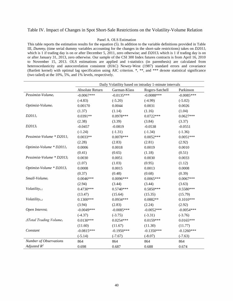
40

Table IV. Impact of Changes in Spot Short-Sale Restrictions on the Volatility-Volume Relation

Panel A. OLS Estimation

This table reports the estimation results for the equation (5). In addition to the variable definitions provided in Table

III, Dummyt (time serial dummy variables accounting for the changes in the short-sale restrictions) takes on D2011t

which is 1 if trading day is on or after December 5, 2011, zero otherwise; and D2013t which is 1 if trading day is on

or after January 31, 2013, zero otherwise. Our sample of the CSI 300 Index futures contracts is from April 16, 2010

to November 15, 2013. OLS estimations are applied and t-statistics (in parenthesis) are calculated from

heteroscedasticity and autocorrelation consistent (HAC) Newey-West (1987) standard errors and covariance

(Bartlett kernel) with optimal lag specification using AIC criterion. *, **, and *** denote statistical significance

(two tailed) at the 10%, 5%, and 1% levels, respectively.




(-4.83) (-5.20) (-4.99) (-5.02)


(1.37) (1.14) (1.16) (1.04)

D2011t 0.0391** 0.0978*** 0.0722*** 0.0627***

(2.38) (3.39) (3.84) (3.37)

D2013t -0.0457 -0.0819 -0.0538 -0.0551

(-1.24) (-1.31) (-1.34) (-1.36)

Pessimist-Volume * D2011t 0.0033** 0.0078*** 0.0052*** 0.0051***

(2.28) (2.83) (2.81) (2.92)

Optimist-Volume * D2011t 0.0006 0.0018 0.0019 0.0010

(0.41) (0.65) (1.18) (0.51)

Pessimist-Volume * D2013t 0.0030 0.0051 0.0030 0.0033

(1.07) (1.03) (0.95) (1.12)


(0.37) (0.48) (0.68) (0.39)

Small-Volumet 0.0046*** 0.0096*** 0.0065*** 0.0067***

(2.94) (3.44) (3.44) (3.63)

Volatilityt-1 0.4730*** 0.5740*** 0.5850*** 0.5580***

(13.47) (15.64) (15.35) (15.79)

Volatilityt-2 0.1300*** 0.0934*** 0.0882** 0.1010***

(3.94) (2.83) (2.24) (2.92)

Open Interestt -0.0049*** -0.0085*** -0.0052*** -0.0054***

(-4.37) (-3.75) (-3.31) (-3.76)


(11.60) (11.67) (11.30) (11.77)

Constant -0.0815*** -0.1950*** -0.1350*** -0.1260***

(-5.14) (-7.67) (-8.07) (-7.63)


Adjusted R2 0.698 0.687 0.688 0.674

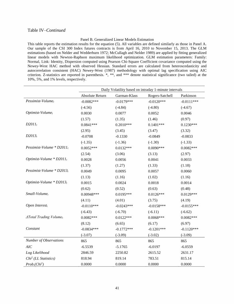
41

Table IV–Continued

Panel B. Generalized Linear Models Estimation

This table reports the estimation results for the equation (5). All variables are defined similarly as those in Panel A.

Our sample of the CSI 300 Index futures contracts is from April 16, 2010 to November 15, 2013. The GLM

estimations (based on Nelder and Wedderburn 1972; McCullagh and Nelder 1989) are applied by fitting generalized

linear models with Newton-Raphson maximum likelihood optimization. GLM estimation parameters: Family:

Normal, Link: Identity, Dispersion computed using Pearson Chi-Square Coefficient covariance computed using the

Newey-West HAC method with observed Hessian. Standard errors are calculated from heteroscedasticity and

autocorrelation consistent (HAC) Newey-West (1987) methodology with optimal lag specification using AIC

criterion. Z-statistics are reported in parenthesis. *, **, and *** denote statistical significance (two tailed) at the

10%, 5%, and 1% levels, respectively.




(-4.56) (-4.84) (-4.80) (-4.67)


(1.57) (1.35) (1.46) (0.97)

D2011t 0.0841*** 0.2010*** 0.1401*** 0.1230***

(2.95) (3.45) (3.47) (3.32)

D2013t -0.0708 -0.1330 -0.0849 -0.0833

(-1.35) (-1.36) (-1.30) (-1.33)

Pessimist-Volume * D2011t 0.0052*** 0.0132*** 0.0090*** 0.0082***

(2.54) (3.06) (3.13) (2.97)


(1.37) (1.27) (1.33) (1.18)

Pessimist-Volume * D2013t 0.0049 0.0095 0.0057 0.0060

(1.13) (1.16) (1.02) (1.16)


(0.62) (0.52) (0.63) (0.48)

Small-Volumet 0.00948*** 0.0195*** 0.0126*** 0.0129***

(4.11) (4.01) (3.75) (4.19)

Open Interestt -0.0110*** -0.0243*** -0.0158*** -0.0155***

(-6.43) (-6.70) (-6.11) (-6.62)


(8.12) (6.65) (6.17) (6.97)

Constant -0.0834*** -0.1772*** -0.1201*** -0.1120***

(-3.07) (-3.09) (-3.02) (-3.09)


AIC -6.5539 -5.1765 -6.0197 -6.0559

Log Likelihood 2846.59 2250.82 2615.52 2631.17

Chi2 (LL Statistics) 818.94 819.14 783.51 815.14

Prob.(Chi2) 0.0000 0.0000 0.0000 0.0000

42

Table V. Pairwise Granger Causality Tests

Panel A. Pessimistic Volume and Volatility

Null Hypothesis F-Statistic Prob.

Pessimist-Volume does not Granger Cause Absolute Return 1.9581 0.0252

Absolute Return does not Granger Cause Pessimist-Volume 0.1253 0.7234

Pessimist-Volume does not Granger Cause Garman-Klass 7.5769 0.0060

Garman-Class does not Granger Cause Pessimist-Volume 0.7831 0.3765

Pessimist-Volume does not Granger Cause Rogers-Satchell 9.4405 0.0022

Rogers-Satchell does not Granger Cause Pessimist-Volume 1.4346 0.2313

Pessimist-Volume does not Granger Cause Parkinson 7.2153 0.0074

Parkinson does not Granger Cause Pessimist-Volume 0.4789 0.4891

Pessimist-Volume does not Granger Cause E-GARCH 41.4155 0.0000

E-GARCH does not Granger Cause Pessimist-Volume 2.1733 0.1408

Pessimist-Volume does not Granger Cause T-GARCH 46.5893 0.0000

T-GARCH does not Granger Cause Pessimist-Volume 1.9705 0.1608

Panel B. Optimistic Volume and Volatility

Null Hypothesis F-Statistic Prob.

Optimist-Volume does not Granger Cause Absolute Return 0.0775 78.1%

Absolute Return does not Granger Cause Optimist-Volume 0.1723 67.8%

Optimist-Volume does not Granger Cause Garman-Klass 1.3786 24.1%

Garman-Class does not Granger Cause Optimist-Volume 1.5853 20.8%

Optimist-Volume does not Granger Cause Rogers-Satchell 2.4875 11.5%

Rogers-Satchell does not Granger Cause Optimist-Volume 2.3953 12.2%

Optimist-Volume does not Granger Cause Parkinson 0.9079 34.1%

Parkinson does not Granger Cause Optimist-Volume 1.3928 23.8%

Optimist-Volume does not Granger Cause E-GARCH 1.50492 11.7%

E-GARCH does not Granger Cause Optimist-Volume 1.81477 10.7%

Optimist-Volume does not Granger Cause T-GARCH 1.57732 16.4%

T-GARCH does not Granger Cause Optimist-Volume 2.0096 15.7%

43

Table VI. Time-varying Conditional Volatility Framework

Panel A. Trading and Time-varying Conditional Volatility of the CSI 300 Index futures

This panel reports the estimation results for the Equations (6) and (7) 0 1 log( )t t tR h , where conditional variance var( )t th is given by

2 2

1 1 1 1 2 3- p q

t i i t j j j t j k k kt t t tSmall Volume Open Interest Total Trading Voh h luVolumeVariable me where VolumeVariablekt are Optimist-Volumet and

Pessimist-Volumet.

Mean Equation

Variable Constant log(ht)

Coefficient 0.01546 0.00175

z-Statistic (3.134)*** (3.253)***

Conditional Variance Equation

Variable Constant ԑ2t-1 ԑ2

t-2 ht-1 ht-2

Pessimist

Volumet

Optimist

Volumet

Small

Volumet

Open

Interestt

ΔTrading

Volumet

DoF Student's

t-distribution

Coefficient 0.00025 0.04485 -0.04088 0.66805 -0.28716 -0.00003250 0.00000036 0.00003950 -0.00009410 0.00015200 7.00

z-Statistic (3.807)*** (2.258)** (-2.56)** (6.598)*** (-3.878)*** (-2.225)** (0.034) (1.957)* (-6.859)*** (8.295)*** (4.684)***

Adjusted R2 0.00357 Log

likelihood 2,777.6

Durbin-

Watson 2.0072

Panel B. Impact of Changes in Spot Short-Sale Restrictions on Time-varying Conditional Volatility-Volume Relation

This panel reports the estimation results for the Equations (6) and (8): 0 1 log( )t t tR h , where conditional variance var( )t th is given by

2 2 2 2 2

1 1 1 1 1 1 1 2 3- d kd t t t

p q

t i i t j j j t j k k kt d dt k d kt dth h VolumeVariable Dummy V Small Volume Open Interest Total TradinolumeVariable Dumm g Volumey

where VolumeVariablekt are Optimist-Volumet and Pessimist-Volumet; Dummyjt variables are D2011t and D2013t.. Our sample of the CSI 300 Index futures contracts is

from April 16, 2010 to November 15, 2013. *, **, and *** denote statistical significance (two tailed) at the 10%, 5%, and 1% levels, respectively.

Mean Equation



z-Statistic (4.078)*** (4.112)***


Variable Constant ԑ2t-1 ht-1

Pessimist

Volumet

Optimist

Volumet

Small

Volumet

Open

Interestt

ΔTrading

Volumet

Pessimist

Vol*D2011t

Pessimist

Vol*D2013t

Optimist

Vol*D2011t

Optimist

Vol*D2013t

DoF Student's

t-distribution

Coefficient 0.00101 0.00698 -0.18282 -0.0000358 0.0000232 0.0000700 -0.00028 0.0000546 0.0000069 0.0000076 0.0000080 -0.0000076 3.43

z-Statistic (3.827)*** (2.359)* (-1.208) (-5.438)*** (0.619) (1.973)** (-7.14)*** (2.835)*** (1.888)** (2.564)** (0.213) (-0.245) (6.517)***

Adjusted

R2 0.00567

Log

likelihood 2,762.6

Durbin-

Watson 2.0097

44

Table VII. Estimation of Asymmetric Time-varying Volatility

Panel A. TGARCH-M(1,1) Model Estimation

This panel reports the estimation results for the Equations (6) and (9): 0 1 log( )t t tR h , where conditional variance is

given var( )t th by 2 2

1 1 1

p q n

t i i t j j j t j k k t k t kh h I

where 1tI if 0t and 0 otherwise. In this model, good

news, 0t i , and bad news, 0t i have differential effects on the conditional variance.

Mean Equation



z-Statistic (2.344)** (2.42)**


Variable Constant ԑ2t-1 ԑ2

t-1*I-t-1 ht-1

Open

Interestt

ΔTrading

Volumet

DoF Student's

t-distribution

Coefficient 0.00023 -0.01567 0.05605 0.48539 -0.000091 0.000067 3.80

z-Statistic (3.106)*** (-5.663)*** (2.267)*** (3.84)*** (-6.891)*** (3.976)*** (6.039)***

Adjusted R2 0.00262 Log likelihood 2,745.0 Durbin-

Watson 1.9951

Panel B. EGARCH-M(1,1) Model Estimation

This panel reports the estimation results for the Equations (6) and (10): , where conditional variance

var( )t th is given by 1 1 11/2 1/2

log( ) log( )p r qt i t kt i i k k j j t j

t i t k

h hh h

where 0t i is good news and 0t i is bad

news. Both asymmetric GARCH models are estimated using log variance as the ARCH in mean parameter, Student’s t

representing the distribution of the errors (with optimal degrees of freedom) based on the BHHH optimization method. Our

sample of the CSI 300 Index futures contracts is from April 16, 2010 to November 15, 2013. *, **, and *** denote statistical

significance (two tailed) at the 10%, 5%, and 1% levels, respectively.

Mean Equation



z-Statistic (3.566)*** (4.618)***


Variable Constant | ԑt-1/h1/2t-1| ԑt-1/h1/2

t-1 log(ht-1)

Open

Interestt

ΔTrading

Volumet

DoF Student's

t-distribution

Coefficient -6.64889 -0.00633 -0.06416 -0.87656 -1.33338 0.39519 3.62

z-Statistic (-3.654)*** (-2.558)** (-3.509)*** (-14.973)*** (-6.875)*** (2.996)*** (6.159)***

Adjusted

R2 0.00197

Log

likelihood 2,745.4

Durbin-

Watson 2.0087

0 1 log( )t t tR h

45

Table VIII. Impact of Changes in Spot Short-Sale Restrictions on the Asymmetric Time-varying

Volatility-Volume Relation

This table reports the estimation results for the equation (5). Volatilityt takes on either TGARCH or EGARCH,

volatility estimates we obtained from asymmetric GARCH models. Again, Pessimist-Volumet is defined as the total

trading volume of investors whose long position in futures is smaller than their short position, i.e., trading firms with

net short position at the end of previous trading day; and Optimist-Volumet is defined as the total trading volume of

investors whose long position in futures is greater than (or equal to) their short position, i.e., trading firms with net

short position at the end of previous trading day., Dummyt (time serial dummy variables accounting for the changes

in the short-sale restrictions) takes on D2011t which is 1 if trading day is on or after December 5, 2011, zero

otherwise; and D2013t which is 1 if trading day is on or after January 31, 2013, zero otherwise. Our sample of the

CSI 300 Index futures contracts is from April 16, 2010 to November 15, 2013. OLS estimations are applied and t-

statistics (in parenthesis) are calculated from heteroscedasticity and autocorrelation consistent (HAC) Newey-West

(1987) standard errors and covariance (Bartlett kernel) with optimal lag specification using AIC criterion. *, **, and

*** denote statistical significance (two tailed) at the 10%, 5%, and 1% levels, respectively.

Time-varying Asymmetric Volatility Estimates

TGARCH Volatility EGARCH Volatility

Pessimist-Volumet -0.0018* -0.0025**

(-1.81) (-2.19)

Optimist-Volumet 0.0029 0.00274

(1.43) (1.56)

D2011t -0.0391*** -0.0408***

(-2.59) (-2.73)

D2013t -0.0361** -0.0224**

(-2.24) (-2.19)

Pessimist-Volume * D2011t 0.0006*** 0.0023***

(2.80) (2.97)

Optimist-Volume * D2011t 0.0046 0.0015

(1.31) (1.10)

Pessimist-Volume * D2013t 0.0008* 0.0001**

(1.87) (2.41)

Optimist-Volume * D2013t -0.0020 0.0006

(-1.57) (0.65)

Small-Volumet 0.0026*** 0.0039***

(2.61) (3.18)

Open Interestt -0.0246*** -0.0236***

(-5.19) (-14.19)

ΔTotal Trading Volumet 0.0081*** 0.0074***

(10.32) (11.15)

Constant 0.1560*** 0.1930***

(2.51) (9.26)

Number of Observations 865 865

Adjusted R2 0.6841 0.6895

46

Table IX. Trader Type and Index Futures Volatility

This table reports the estimation results for the equation (11). Trading Member (Clearing Member) Pessimist-

Volume represent the trading volume by pessimist exchange member types and Trading Member (Clearing Member)

Optimist-Volume represent the trading volume by optimist exchange member types, as defined in Section 4.1. Our

sample of the CSI 300 Index futures contracts is from April 16, 2010 to November 15, 2013. OLS estimations are

applied and t-statistics (in parenthesis) are calculated from heteroscedasticity and autocorrelation consistent (HAC)

Newey-West (1987) standard errors and covariance (Bartlett kernel) with optimal lag specification using AIC

criterion. *, **, and *** denote statistical significance (two tailed) at the 10%, 5%, and 1% levels, respectively.



Trading Member, Pessimist-Volumet -0.000428*** -0.000222*** -0.000152** -0.000116***

(-2.76) (-3.23) (-2.33) (-2.79)

Clearing Member, Pessimist-Volumet 0.000477 0.000122** 0.000818** 0.000583*

(0.63) (2.42) (2.13) (1.86)

Trading Member, Optimist-Volumet -0.000014 0.000375 0.000025 0.000023

(-0.57) (0.79) (0.78) (0.59)

Clearing Member, Optimist-Volumet 0.000045 0.000157 0.000102 0.000756

(0.71) (1.24) (1.22) (0.93)

Volatilityt-1 0.4781*** 0.5780*** 0.5934*** 0.5596***

(13.58) (15.68) (15.50) (15.21)

Volatilityt-2 0.1350*** 0.0940*** 0.0872*** 0.1010***

(4.44) (3.03) (2.68) (3.26)

Small-Volumet 0.0097*** 0.0188*** 0.0120*** 0.0124***

(11.50) (11.89) (11.28) (12.12)

Open Interestt -0.0075*** -0.0153*** -0.0100*** -0.0099***

(-8.59) (-8.91) (-8.52) (-9.12)


(11.44) (11.20) (10.87) (11.23)

Constant -0.0261*** -0.0497*** -0.0297*** -0.0327***

(-4.33) (-4.50) (-4.03) (-4.62)


Adjusted R2 0.677 0.733 0.728 0.723

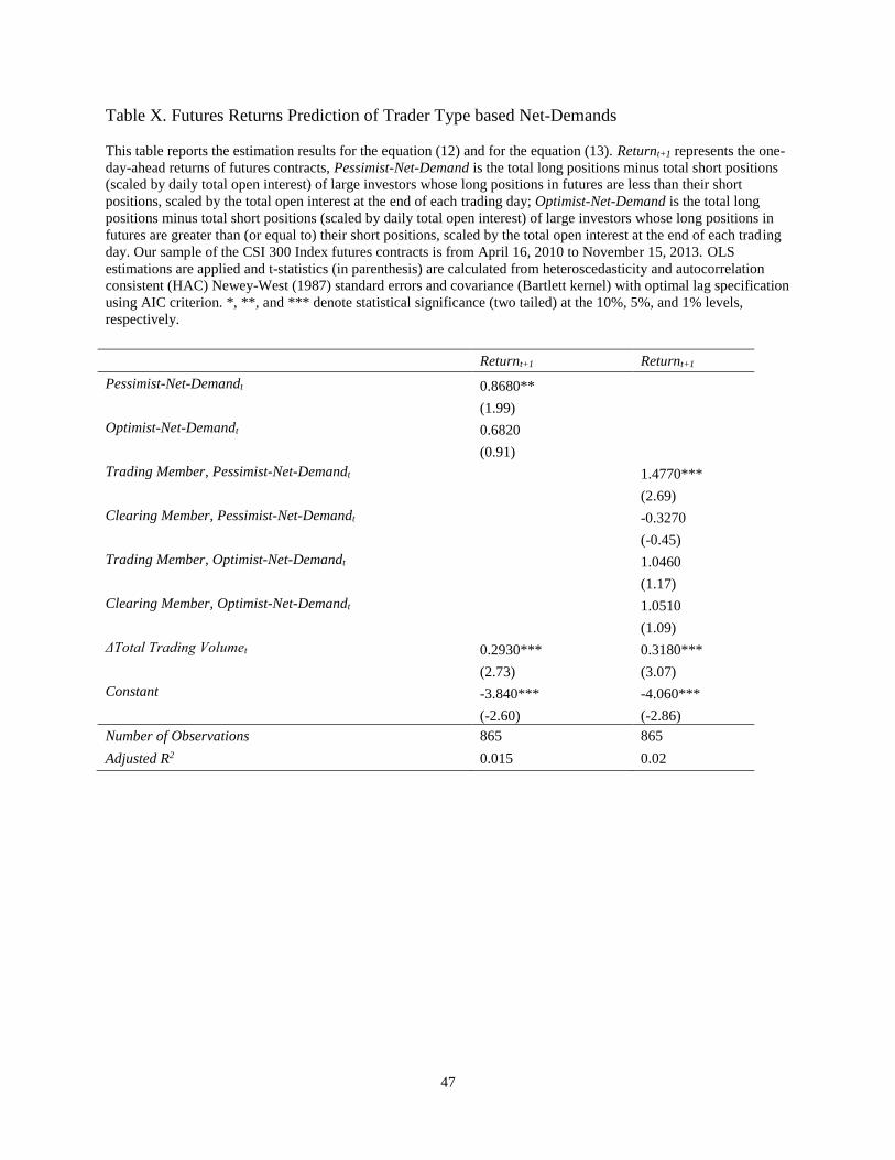
47

Table X. Futures Returns Prediction of Trader Type based Net-Demands

This table reports the estimation results for the equation (12) and for the equation (13). Returnt+1 represents the one-

day-ahead returns of futures contracts, Pessimist-Net-Demand is the total long positions minus total short positions

(scaled by daily total open interest) of large investors whose long positions in futures are less than their short

positions, scaled by the total open interest at the end of each trading day; Optimist-Net-Demand is the total long

positions minus total short positions (scaled by daily total open interest) of large investors whose long positions in

futures are greater than (or equal to) their short positions, scaled by the total open interest at the end of each trading

day. Our sample of the CSI 300 Index futures contracts is from April 16, 2010 to November 15, 2013. OLS

estimations are applied and t-statistics (in parenthesis) are calculated from heteroscedasticity and autocorrelation

consistent (HAC) Newey-West (1987) standard errors and covariance (Bartlett kernel) with optimal lag specification

using AIC criterion. *, **, and *** denote statistical significance (two tailed) at the 10%, 5%, and 1% levels,

respectively.

Returnt+1 Returnt+1

Pessimist-Net-Demandt 0.8680**

(1.99) Optimist-Net-Demandt 0.6820

(0.91) Trading Member, Pessimist-Net-Demandt

1.4770***

(2.69)

Clearing Member, Pessimist-Net-Demandt -0.3270

(-0.45)

Trading Member, Optimist-Net-Demandt 1.0460

(1.17)

Clearing Member, Optimist-Net-Demandt 1.0510

(1.09)

ΔTotal Trading Volumet 0.2930*** 0.3180***

(2.73) (3.07)

Constant -3.840*** -4.060***

(-2.60) (-2.86)

Number of Observations 865 865

Adjusted R2 0.015 0.02

48

Figure 1. CSI 300 Stock Index Level and Spot Trading Volume. Source: Bloomberg. Our sample is from April 16,

2010 to November 15, 2013.

2,000

4,000

6,000

8,000

10,000

12,000

14,000

16,000

18,000

20,000

22,000

2,000

2,200

2,400

2,600

2,800

3,000

3,200

3,400

3,600

Trad

ing

Vo

lum

e (

shar

es

in m

illio

ns)

CSI

30

0 In

dex

Lev

el

CSI 300 Index Level Trading Volume (shares in millions)

frank j. fabozzi edhec business school - weebly

Documents