fraptran-2.0: a computer code for the transient … code for the transient analysis of oxide fuel...

PNNL-19400, Vol.1 Rev2

Prepared for the U.S. Department of Energy under Contract DE-AC05-76RL01830

FRAPTRAN-2.0: A Computer Code for the Transient Analysis of Oxide Fuel Rods May 2016

KJ Geelhood WG Luscher JM Cuta IA Porter

PNNL-19400, Vol.1 Rev2

FRAPTRAN-2.0: A Computer Code for the Transient Analysis of Oxide Fuel Rods KJ Geelhood WG Luscher JM Cuta IA Porter May 2016 Prepared for the U.S. Department of Energy under Contract DE-AC05-76RL01830 Pacific Northwest National Laboratory Richland, Washington 99352

iii

Abstract

The Fuel Rod Analysis Program Transient (FRAPTRAN) is a Fortran language computer code that calculates the transient performance of light-water reactor fuel rods during reactor transients and hypothetical accidents such as loss-of-coolant accidents, anticipated transients without scram, and reactivity-initiated accidents. FRAPTRAN calculates the temperature and deformation history of a fuel rod as a function of time-dependent fuel rod power and coolant boundary conditions. Although FRAPTRAN can be used in “standalone” mode, it is often used in conjunction with, or with input from, other codes. The phenomena modeled by FRAPTRAN include a) heat conduction, b) heat transfer from cladding to coolant, c) elastic-plastic fuel and cladding deformation, d) cladding oxidation, e) fission gas release, and f) fuel rod gas pressure. FRAPTRAN is programmed for use on Windows-based computers but the source code may be compiled on any other computer with a Fortran 2008 and newer compiler.

Burnup-dependent parameters may be initialized from the FRAPCON steady-state single rod fuel performance code.

This document describes FRAPTRAN-2.0, which is the latest version of FRAPTRAN.

v

Foreword

Computer codes related to fuel performance have played an important role in the work of the U.S. Nuclear Regulatory Commission (NRC) since the agency’s inception in 1975. Formal requirements for fuel performance analysis appear in several of the agency’s regulatory guides and regulations, including those related to emergency core cooling system evaluation models, as set forth in Appendix K to Title 10, Part 50, of the Code of Federal Regulations (10 CFR Part 50), “Domestic Licensing of Production and Utilization Facilities.”

This document describes the latest version of NRC’s transient fuel performance code, FRAPTRAN-2.0 (Fuel Rod Analysis Program Transient). This code provides the ability to accurately calculate the performance of light-water reactor fuel during both long-term steady-state and various operational transients and hypothetical accidents, accomplishing a key objective of the NRC’s reactor safety research program. FRAPTRAN is also a companion code to the FRAPCON code (Geelhood et al. 2015), developed to calculate the steady-state high burnup response of a single fuel rod.

The latest version of FRAPTRAN has been re-written to use modern FORTRAN language. As part of this update, some minor coding errors were corrected. .

vii

Executive Summary

The fuel performance code, FRAPTRAN, has been developed for the U.S. Nuclear Regulatory Commission (NRC) by Pacific Northwest National Laboratory for calculating transient fuel behavior at high burnup (up to 62 gigawatt-days per metric ton of uranium). The code has been significantly modified since the release of FRAPTRAN v1.0 in 2001. This document is Volume 1 of a two-volume series that describes the current version, FRAPTRAN-2.0. This document 1) describes the code structure and limitations, 2) summarizes the fuel performance models, and 3) provides the code input instructions and features to aid the user. Volume 2 (Geelhood and Luscher 2016) is a code assessment based on comparisons of code predictions to fuel rod integral performance data up to high burnup levels. Basic fuel, cladding, and gas material properties are provided in a separate material properties handbook (Luscher and Geelhood 2015).

FRAPTRAN is designed to perform transient fuel rod thermal and mechanical calculations. Transient initial conditions due to steady-state operation can be obtained from the companion FRAPCON steady-state fuel rod performance code. FRAPTRAN uses a finite difference heat conduction model that uses a variable mesh spacing to accommodate the power peaking that occurs at the pellet edge in high burnup fuel. A new model for fuel thermal conductivity that includes the effect of burnup degradation has been incorporated, as have new cladding mechanical property models that account for the effect of high burnup. The code uses the same material properties package as does the steady-state NRC fuel code, FRAPCON.

ix

Acronyms and Abbreviations

°C degrees Celsius °F degrees Fahrenheit ANS American Nuclear Society Btu British thermal unit(s) BWR boiling-water reactor cal/mol calories per mole CHF critical heat flux cm centimeters cm2 square centimeter(s) crud Chalk River Unidentified Deposit (generic term for various residues deposited on

fuel rod surfaces, originally coined by Atomic Energy of Canada, Ltd. to describe deposits observed on fuel from the test reactor at Chalk River)

DNB departure from nucleate boiling ECR equivalent cladding reacted FEA finite element analysis FRAP-T Fuel Rod Analysis Program-Transient FRAPTRAN Fuel Rod Analysis Program Transient ft foot/feet ft2 square foot/feet ft3 cubic foot/feet g gram(s) Gd2O3 gadolinia GWd/MTU gigawatt-days per metric ton of uranium hr hour(s) ID inner diameter J joule(s) K kelvin kg kilogram(s) kW kilowatt(s) lbf pound-force lbm pound-mass LOCA loss-of-coolant accident LWR light-water reactor m meter(s) m2 square meter(s) m3 cubic meter(s)

x

Mlbm megapound-mass mol mole(s) MOX mixed-oxide fuel MPa megapascal(s) MW megawatt(s) MWd/MTM megawatt-days per metric ton of metal MWd/MTU megawatt-days per metric ton of uranium MWs megawatt-seconds MWs/kg megawatt-seconds per kilogram n neutron(s) N newton(s) NRC U.S. Nuclear Regulatory Commission OD outer diameter PCMI pellet/cladding mechanical interaction PNNL Pacific Northwest National Laboratory ppm part(s) per million psia pound(s) per square inch absolute PWR pressurized-water reactor RIA reactivity-initiated accident s second(s) SI International System of Units TD theoretical density UO2 uranium dioxide UO2-Gd2O3 urania-gadolinia W watt(s) μin microinch(es) μm micrometer(s)

xi

Contents

Abstract ........................................................................................................................................................ iii Foreword ....................................................................................................................................................... v Executive Summary .................................................................................................................................... vii Acronyms and Abbreviations ...................................................................................................................... ix 1.0 Introduction ....................................................................................................................................... 1.1

1.1 Objectives and Scope of the FRAPTRAN Code ....................................................................... 1.1 1.2 Relation to Other NRC Codes ................................................................................................... 1.3 1.3 Report Outline and Relation to Other Reports .......................................................................... 1.5

2.0 General Modeling Descriptions ......................................................................................................... 2.1 2.1 Order and Interaction of Models ............................................................................................... 2.1 2.2 Fuel and Cladding Temperature Model ..................................................................................... 2.3

2.2.1 Local Coolant Conditions ............................................................................................... 2.5 2.2.2 Heat Generation .............................................................................................................. 2.5 2.2.3 Gap Conductance ........................................................................................................... 2.5 2.2.4 Fuel Thermal Conductivity ............................................................................................ 2.7 2.2.5 Fuel Rod Cooling ........................................................................................................... 2.9 2.2.6 Heat Conduction and Temperature Solution ................................................................ 2.12

2.3 Plenum Gas Temperature Model ............................................................................................. 2.17 2.3.1 Plenum Temperature Equations ................................................................................... 2.17 2.3.2 Heat Conduction Coefficients ...................................................................................... 2.22

2.4 Fuel Rod Mechanical Response Model ................................................................................... 2.27 2.4.1 General Considerations in Elastic-Plastic Analysis ..................................................... 2.27 2.4.2 Extension to Creep and Hot Pressing ........................................................................... 2.32 2.4.3 Rigid Pellet Model (FRACAS-I) .................................................................................. 2.34 2.4.4 Cladding Ballooning Model ......................................................................................... 2.52

2.5 Fuel Rod Internal Gas Pressure Response Model ................................................................... 2.57 2.5.1 Static Fuel Rod Internal Gas Pressure .......................................................................... 2.58 2.5.2 Transient Internal Gas Flow ......................................................................................... 2.59 2.5.3 Fission Gas Production and Release ............................................................................ 2.61

2.6 High-Temperature Corrosion .................................................................................................. 2.62 2.7 Fuel Radial Thermal Expansion Routine ................................................................................ 2.63 2.8 Cladding Failure Models ......................................................................................................... 2.64

2.8.1 Low-Temperature PCMI Cladding Failure Model ....................................................... 2.64 2.8.2 High-Temperature Cladding Ballooning Failure Model .............................................. 2.66

3.0 User Information................................................................................................................................ 3.1 3.1 Code Structure and Solution Routine ........................................................................................ 3.1

xii

3.2 Input Information ...................................................................................................................... 3.3 3.3 Output Information .................................................................................................................... 3.7 3.4 Nodalization, Accuracy, and Computation Time Considerations ............................................. 3.8 3.5 Comments and Guidance on Operating FRAPTRAN ............................................................. 3.10

4.0 References ......................................................................................................................................... 4.1 Appendix A – Input Instructions for FRAPTRAN ................................................................................... A.1 Appendix B – Input Option for Data File with Transient Coolant Conditions ..........................................B.1 Appendix C – Calculation of Cladding Surface Temperature ...................................................................C.1 Appendix D – Heat Transfer Correlations and Coolant Models ............................................................... D.1 Appendix E – Numerical Solution of the Plenum Energy Equations ........................................................ E.1 Appendix F – High-Temperature Oxidation Models in FRAPTRAN-2.0 ................................................. F.1

xiii

Figures

Figure 1.1. Schematic of Typical LWR Fuel Rod .................................................................................... 1.2 Figure 1.2. Locations at Which Fuel Rod Variables are Evaluated .......................................................... 1.4 Figure 2.1. Order of General Models ........................................................................................................ 2.3 Figure 2.2. Flowchart of Fuel and Cladding Temperature Model ............................................................ 2.4 Figure 2.3. Relation of Surface Heat Flux to Surface Temperature ........................................................ 2.10 Figure 2.4. Description of Geometry Terms in Finite Difference Equations for Heat Conduction ........ 2.14 Figure 2.5. Energy Flow in Plenum Model – Spring Model with Two Nodes ....................................... 2.17 Figure 2.6. Energy Flow in Plenum Model – Energy Exchange Mechanisms ....................................... 2.18 Figure 2.7. Flowchart of Plenum Temperature Calculation .................................................................... 2.19 Figure 2.8. Cladding Noding .................................................................................................................. 2.20 Figure 2.9. Geometrical Relationship Between the Cladding and Spring .............................................. 2.25 Figure 2.10. Typical Isothermal True Stress-strain Curve ...................................................................... 2.29 Figure 2.11. Schematic of the Method of Successive Elastic Solutions ................................................. 2.33 Figure 2.12. Fuel Rod Geometry and Coordinates ................................................................................. 2.36

Figure 2.13. Calculation of Increment of Plastic Strain, dε P, from Effective Stress, σe ........................ 2.38 Figure 2.14. True Stress-strain Curve and Unloading Path .................................................................... 2.43 Figure 2.15. Computing Stress ................................................................................................................ 2.45 Figure 2.16. Axial Thermal Expansion Using FRACAS-I ..................................................................... 2.50 Figure 2.17. Description of the BALON2 Model ................................................................................... 2.53 Figure 2.18. True Hoop Stress at Burst that is Used in BALON2 and FRAPTRAN ............................. 2.54 Figure 2.19. Engineering Burst Stress Data and FRAPTRAN Predictions for Low Heating Rates ....... 2.55 Figure 2.20. Engineering Burst Stress Data and FRAPTRAN Predictions for High Heating Rates ...... 2.55 Figure 2.21. Permanent Burst Strain Data and FRAPTRAN Predictions for Low Temperature Ramp

Rates 2.56 Figure 2.22. Permanent Burst Strain Data and FRAPTRAN Predictions for High Temperature Ramp

Rates 2.57 Figure 2.23. Internal Pressure Distribution with the Gas Flow Model ................................................... 2.60 Figure 2.24. Hagen Number Versus Width of Fuel-Cladding Gap ......................................................... 2.61 Figure 3.1. Flowchart of FRAPTRAN (Part 1) ......................................................................................... 3.2 Figure 3.2. Flowchart of FRAPTRAN (Part 2) ......................................................................................... 3.2 Figure 3.3. Flowchart of FRAPTRAN (Part 3) ......................................................................................... 3.3 Figure 3.4. Example of Fuel Rod Nodalization ........................................................................................ 3.9 Figure A.1. Example of Input Data File Illustrating Necessary Data Lines ............................................ A.3 Figure A.2. Illustration of How Time Step Size and Power History are Interpreted by FRAPTRAN .. A.43 Figure A.3. Illustration of Node Location for Five Evenly Spaced Axial Nodes .................................. A.44 Figure A.4. Illustration of Nodal Location for Five Unevenly Spaced Axial Nodes ............................. A.45

xiv

Figure B.1. Example Geometry for Input of Coolant Channel Data .........................................................B.3 Figure D.1. Illustration of FRAPTRAN Forced Convection Heat Transfer Regimes for Full Boiling

Curve D.40 Figure D.2. Description of Geometry Terms in Coolant Enthalpy Model ............................................. D.41 Figure F.1. Comparison of C-P and B-J Models at Temperatures from 600 to 1400°C ........................... F.3

Figure F.2. Comparison of C-P and B-J Models to Data at Temperatures from 600 to 800°C ................ F.4

xv

Tables

Table 1.1. Roadmap to Documentation of Models and Properties in NRC Fuel Performance Codes, FRAPCON-4.0 and FRAPTRAN-2.0 ................................................................................................ 1.6

Table 2.1. Heat Transfer Mode Selection and Correlations .................................................................... 2.10 Table 2.2. Nomenclature for Plenum Thermal Model ............................................................................ 2.21 Table 2.3. Elastic-plastic Governing Equations ...................................................................................... 2.32 Table 2.4. Constants for Cathcart-Pawel and Baker-Just Models ........................................................... 2.63 Table 2.5. Predicted Minus Measured Uniform Elongation from Irradiated Samples from the PNNL

Database as a Function of Excess Hydrogen ................................................................................... 2.65 Table 3.1. Name and Function of Principal FRAPTRAN Subcodes ........................................................ 3.1 Table 3.2. Input Information ..................................................................................................................... 3.4 Table 3.3. Variables Written by FRAPCON and Read by FRAPTRAN for Burnup Initialization .......... 3.5 Table 3.4. FRAPTRAN Output Information ............................................................................................ 3.8 Table A.1. $begin Data Block .................................................................................................................. A.6 Table A.2. $iodata Data Block ................................................................................................................. A.7 Table A.3. $solution Data Block .............................................................................................................. A.9 Table A.4. $design Data Block .............................................................................................................. A.12 Table A.5. $power Data Block............................................................................................................... A.17 Table A.6. $model Data Block............................................................................................................... A.20 Table A.7. Recommendations for Modeling Thermal Hydraulic Boundary Conditions for Various CasesA.30 Table A.8. $boundary Data Block ......................................................................................................... A.30 Table A.9. $uncertianties Data Block .................................................................................................... A.42 Table A.10. Recommended Time Step Sizes for Various Transients .................................................... A.42 Table A.11. Definition of Coolant Channel Geometry Terms ............................................................... A.43 Table D.1. Optimized Constants for EPRI-1 CHF Correlation ............................................................. D.12 Table D.2. Coefficients for MacBeth’s 6-coefficient Model ................................................................. D.18 Table D.3. Coefficients for MacBeth’s 12-coefficient Model ............................................................... D.19 Table D.4. Coefficient Values for Groeneveld Film Boiling Correlation .............................................. D.31 Table D.5. Chen’s Reynolds Number Factor, F .................................................................................... D.38 Table D.6. The Chen Suppression Factor, S .......................................................................................... D.39 Table D.7. Range of Applicability of Generalized FLECHT Correlation ............................................. D.39 Table D.8. Variable and Symbol Definitions in FLECHT Correlation ................................................. D.40 Table F.1. Constants for Cathcart-Pawel and Baker-Just Models ............................................................ F.5 Table F.2. High-Temperature Oxidation Outputs from FRAPTRAN-2.0 ................................................ F.5

1.1

1.0 Introduction

The ability to accurately calculate the performance of light-water reactor (LWR) fuel during irradiation, and during both long-term steady-state and various operational transients and hypothetical accidents, is an objective of the reactor safety research program being conducted by the U.S. Nuclear Regulatory Commission (NRC). To achieve this objective, the NRC has sponsored an extensive program of analytical computer code development and both in-reactor and out-of-reactor experiments to generate the data necessary for development and verification of the computer codes.

This report provides a description of the FRAPTRAN (Fuel Rod Analysis Program Transient) code, developed to calculate the response of single fuel rods to operational transients and hypothetical accidents at burnup levels up to 62 gigawatt-days per metric ton of uranium (GWd/MTU). This document describes the latest version, FRAPTRAN-2.0. The FRAPTRAN code is the successor to the FRAP-T (Fuel Rod Analysis Program-Transient) code series developed in the 1970s and 1980s (Siefken et al. 1981; Siefken et al. 1983). FRAPTRAN is also a companion code to the FRAPCON-3 code (Geelhood and Luscher 2014a), developed to calculate the steady-state high burnup response of a single fuel rod.

This document, Volume 1 of a two-volume series, describes the code structure and limitations, summarizes the fuel performance models, and provides the code input instructions. Volume 2 (Geelhood and Luscher 2014b) provides the code assessment based on comparisons of code predictions to fuel rod integral performance data up to high burnup (62 GWd/MTU). A separate material properties handbook (Luscher and Geelhood 2014) documents fuel, cladding, and gas material properties used in FRAPCON-4.0 and FRAPTRAN-2.0.

1.1 Objectives and Scope of the FRAPTRAN Code

FRAPTRAN is an analytical tool that calculates LWR fuel rod behavior when power or coolant boundary conditions, or both, are rapidly changing. This is in contrast to the FRAPCON-3 code, which calculates the time (burnup) dependent behavior when power and coolant boundary condition changes are sufficiently slow for the term “steady-state” to apply. FRAPTRAN calculates the variation with time, power, and coolant conditions of fuel rod variables such as fuel and cladding temperatures, cladding elastic and plastic stress and strain, cladding oxidation, and fuel rod gas pressure. Variables that are slowly varying with time (burnup), such as fuel densification and swelling, and cladding creep and irradiation growth, are not calculated by FRAPTRAN. However, the state of the fuel rod at the time of a transient, which is dependent on those variables not calculated by FRAPTRAN, may be read from a file generated by FRAPCON or manually entered by the user.

FRAPTRAN and FRAPCON have not been combined into a single code primarily due to the high cost associated with this effort. Also, FRAPCON is primarily used as an audit tool in the review of vendor fuel performance codes, which happens frequently. FRAPTRAN is not frequently used in licensing applications. FRAPTRAN has primarily been used only in the development of licensing limits for design-basis accident scenarios.

FRAPTRAN is a research tool for 1) analysis of fuel response to postulated design-basis accidents such as reactivity-initiated accidents (RIAs), boiling-water reactor (BWR) power and coolant oscillations without scram, and loss-of-coolant accidents (LOCAs); 2) understanding and interpreting experimental results; and 3) guiding of planned experimental work. Examples of planned applications for FRAPTRAN include defining transient performance limits, identifying data or models needed for understanding transient fuel performance, and assessing the effect of fuel design changes such as new cladding alloys

1.2

and mixed-oxide (MOX) fuel ((U,Pu)O2) on accidents. FRAPTRAN will be used to perform sensitivity analyses of the effects of parameters such as fuel-cladding gap size, rod internal gas pressure, and cladding ductility and strength on the response of a fuel rod to a postulated transient. Fuel rod responses of interest include cladding strain, failure/rupture, location of ballooning, cladding oxidation, etc.

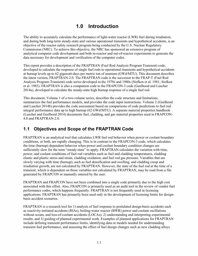
An LWR fuel rod typically consists of oxide fuel pellets enclosed in zirconium alloy cladding, as shown in Figure 1.1. The primary function of the cladding is to contain the fuel column and the radioactive fission products. If the cladding does not crack, rupture, or melt during a reactor transient, the radioactive fission products are contained within the fuel rod. During some reactor transients and hypothetical accidents, however, the cladding may be weakened by a temperature increase, embrittled by oxidation, or overstressed by mechanical interaction with the fuel. These events alone or in combination can cause cracking or rupture of the cladding and release of the radioactive products to the coolant. Furthermore, the rupture or melting of the cladding of one fuel rod can alter the flow of reactor coolant and reduce the cooling of neighboring fuel rods. This event can lead to the loss of a “coolable” reactor core geometry.

Figure 1.1. Schematic of Typical LWR Fuel Rod

Most reactor operational transients and hypothetical accidents will adversely influence the performance of the fuel rod cladding. During an operational transient such as a turbine trip without bypass (for BWRs), the reactor power may temporarily increase and cause an increase in the thermal expansion of the fuel,

1.3

which can lead to the mechanical interaction of the fuel and cladding and overstress the cladding. During an operational transient such as a loss-of-flow event, the coolant flow decreases, which may lead to film boiling on the cladding surface and an increase in the cladding temperature. During a LOCA, the initial stored energy from operation and heat generated by the radioactive decay of fission products is not adequately removed by the coolant and the cladding temperature increases. The temperature increase weakens the cladding and may also lead to cladding oxidation, which embrittles the cladding.

The FRAPTRAN code can model the phenomena which influence the performance of fuel rods in general and the temperature, embrittlement, and stress and strain of the cladding in particular. The code has a heat conduction model to calculate the transfer of heat from the fuel to the cladding and a cooling model to calculate the transfer of heat from the cladding to the coolant. The code has an oxidation model to calculate the extent of cladding embrittlement and the amount of heat generated by cladding oxidation. A mechanical response model is included to calculate the stress and strain applied to the cladding by the mechanical interaction of the fuel and cladding, by the pressure of the gases inside the rod, and by the pressure of the external coolant.

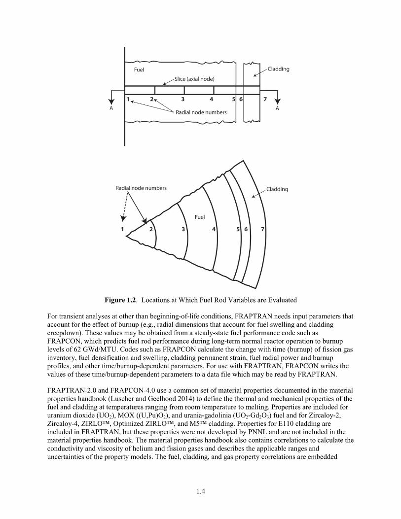
The models in FRAPTRAN use finite difference techniques to calculate the variables which influence fuel rod performance. The variables are calculated at user-specified slices of the fuel rod, as shown in Figure 1.2. Each slice is at a different axial elevation and is defined to be an axial node. At each axial node, the variables are calculated at user-specified radial locations. Each location is at a different radius and is defined to be a radial node. The variables at any given axial node are assumed to be independent of the variables at all other axial nodes (stacked one-dimensional solution, also known as a 1-D1/2 solution).

The FRAPTRAN code was developed at Pacific Northwest National Laboratory (PNNL). FRAPTRAN v1.0 was released first (Cunningham et al. 2001). Since then, six updated versions have been released: FRAPTRAN 1.1, FRAPTRAN 1.1.1, FRAPTRAN 1.2, FRAPTRAN 1.3, FRAPTRAN 1.4, and FRAPTRAN-2.0.

1.2 Relation to Other NRC Codes

FRAPTRAN is the successor to FRAP-T6 (Siefken et al. 1981; Siefken et al. 1983) and is based on FRAP-T6. Major changes incorporated in FRAPTRAN include burnup-dependent material properties and models, simplification of the code, and correction of errors identified since FRAP-T6 was issued. The transient fuel performance code, FRAPTRAN, and the steady-state fuel performance code, FRAPCON, are related in two ways: 1) FRAPTRAN and FRAPCON use the same material properties correlations, and 2) FRAPCON can create an initialization file that can be read by FRAPTRAN to initialize the burnup-dependent parameters in FRAPTRAN before a transient analysis. Although critical heat flux (CHF) and post-CHF correlations are modeled by the code, this is not intended to replace sub-channel codes, such as VIPRE (Stewart et al. 1998) or COBRA (Basile et al. 1999), that provide more accurate modeling for departure from nucleate boiling (DNB) or post-DNB.

1.4

Figure 1.2. Locations at Which Fuel Rod Variables are Evaluated

For transient analyses at other than beginning-of-life conditions, FRAPTRAN needs input parameters that account for the effect of burnup (e.g., radial dimensions that account for fuel swelling and cladding creepdown). These values may be obtained from a steady-state fuel performance code such as FRAPCON, which predicts fuel rod performance during long-term normal reactor operation to burnup levels of 62 GWd/MTU. Codes such as FRAPCON calculate the change with time (burnup) of fission gas inventory, fuel densification and swelling, cladding permanent strain, fuel radial power and burnup profiles, and other time/burnup-dependent parameters. For use with FRAPTRAN, FRAPCON writes the values of these time/burnup-dependent parameters to a data file which may be read by FRAPTRAN.

FRAPTRAN-2.0 and FRAPCON-4.0 use a common set of material properties documented in the material properties handbook (Luscher and Geelhood 2014) to define the thermal and mechanical properties of the fuel and cladding at temperatures ranging from room temperature to melting. Properties are included for uranium dioxide (UO2), MOX ((U,Pu)O2), and urania-gadolinia (UO2-Gd2O3) fuel and for Zircaloy-2, Zircaloy-4, ZIRLO™, Optimized ZIRLO™, and M5™ cladding. Properties for E110 cladding are included in FRAPTRAN, but these properties were not developed by PNNL and are not included in the material properties handbook. The material properties handbook also contains correlations to calculate the conductivity and viscosity of helium and fission gases and describes the applicable ranges and uncertainties of the property models. The fuel, cladding, and gas property correlations are embedded

1.5

within FRAPTRAN so that the code user does not have to supply any material properties. A separate file containing water property data is included with FRAPTRAN.

1.3 Report Outline and Relation to Other Reports

This report serves as both the model description document and the user input manual. A description of the analytical models is provided in Section 2. The overall structure of the code, the input and output information, and the user’s means of controlling computational accuracy and run time are summarized in Section 3 along with some guidance on using the code. A description of the required control and input data is provided in Appendix A. An option for providing transient coolant conditions directly from a file is provided in Appendix B. Provided in Appendices C and D are additional details on the heat transfer models and correlations. A description of the numerical scheme for calculating plenum temperatures is provided in Appendix E. The subroutines that compose each subcode in FRAPTRAN are provided in Appendix F.

This document describes the latest version of FRAPTRAN, FRAPTRAN-2.0.

This report does not present an assessment of the code performance with respect to in-reactor data. Critical comparisons with experimental data from well-characterized, instrumented test rods are presented in Volume 2 of this series, FRAPTRAN-2.0 Integral Assessment (Geelhood and Luscher 2016).

The full documentation of the steady-state and transient fuel performance codes is described in three documents. The basic fuel, cladding, and gas material properties used in FRAPCON-4.0 and FRAPTRAN-2.0 are described in the material properties handbook (Luscher and Geelhood 2015). The FRAPCON-4.0 code structure and behavioral models are described in the FRAPCON-4.0 code description document (Geelhood et al 2015). The FRAPTRAN-2.0 code structure and behavioral models are described in the FRAPTRAN-2.0 code description document (this document).

Table 1.1 shows where each specific material property and model used in the NRC fuel performance codes are documented.

1.6

Table 1.1. Roadmap to Documentation of Models and Properties in NRC Fuel Performance Codes, FRAPCON-4.0 and FRAPTRAN-2.0

Model/Property FRAPCON-4.0 FRAPTRAN-2.0 Fuel thermal conductivity Material properties handbook Material properties handbook Fuel thermal expansion Material properties handbook Material properties handbook Fuel melting temperature Material properties handbook Material properties handbook Fuel specific heat Material properties handbook Material properties handbook Fuel enthalpy Material properties handbook Material properties handbook Fuel emissivity Material properties handbook Material properties handbook Fuel densification Material properties handbook NA Fuel solid swelling Material properties handbook NA Fuel gaseous swelling Material properties handbook NA Fission gas release FRAPCON code description FRAPTRAN code description Fuel relocation FRAPCON code description FRAPTRAN code description Fuel grain growth FRAPCON code description NA High burnup rim model FRAPCON code description NA Nitrogen release FRAPCON code description NA Helium release FRAPCON code description NA Radial power profile FRAPCON code description NA (input parameter) Stored energy FRAPCON code description FRAPTRAN code description Decay heat model NA FRAPTRAN code description Fuel and cladding temperature solution

FRAPCON code description FRAPTRAN code description

Cladding thermal conductivity Material properties handbook Material properties handbook Cladding thermal expansion Material properties handbook Material properties handbook Cladding elastic modulus Material properties handbook Material properties handbook Cladding creep model Material properties handbook NA Cladding specific heat Material properties handbook Material properties handbook Cladding emissivity Material properties handbook Material properties handbook Cladding axial growth Material properties handbook NA Cladding Meyer hardness Material properties handbook Material properties handbook Cladding annealing FRAPCON code description FRAPTRAN code description Cladding yield stress and plastic deformation


Cladding failure criteria NA FRAPTRAN code description Cladding waterside corrosion FRAPCON code description NA (input parameter) Cladding hydrogen pickup FRAPCON code description NA (input parameter) Cladding high temperature oxidation

NA FRAPTRAN code description

Cladding ballooning model NA FRAPTRAN code description Cladding mechanical deformation FRAPCON code description FRAPTRAN code description Oxide thermal conductivity Material properties handbook Material properties handbook

1.7

Model/Property FRAPCON-4.0 FRAPTRAN-2.0 Crud thermal conductivity FRAPCON code description NA Gas conductivity Material properties handbook Material properties handbook Gap conductance FRAPCON code description FRAPTRAN code description Plenum gas temperature FRAPCON code description FRAPTRAN code description Rod internal pressure FRAPCON code description FRAPTRAN code description Coolant temperature and heat transfer coefficients


Optional models and properties not developed at PNNL VVER fuel and cladding models NA NUREG/IA-0164

(Shestopalov et al. 1999) Cladding FEA model VTT-R-11337-06

(Knuttilla 2006) VTT-R-11337-06 (Knuttilla 2006)

FEA = finite element analysis NA = not applicable VVER = water-cooled, water-moderated energy reactor

2.1

2.0 General Modeling Descriptions

Several phenomenological models are required to calculate the transient performance of fuel rods. Models are included in FRAPTRAN to calculate a) heat conduction, b) cladding stress and strain, and c) rod internal gas pressure. Each of these general models is composed of several specific models. For example, the heat conduction model includes models of a) the conduction of heat across the fuel-cladding gap, b) the transfer of heat from the cladding to the coolant, and c) the conduction of heat in a composite cylinder.

This section of the report first describes the order and interaction of the various models. Then the details of each model are discussed. This discussion includes a) a list of the assumptions upon which the model is based, b) the dependent and independent variables in each model, and c) the equations used to solve for the values of the dependent variables.

2.1 Order and Interaction of Models

The order of the general models in FRAPTRAN is shown in Figure 2.1. The solution for the fuel rod variables begins with the calculation of the temperatures of the fuel and cladding. The temperature of the gases in the fuel rod is then calculated. Next, the stresses and strains in the fuel and cladding are calculated. The pressure of the gas inside the fuel rod is then calculated, including the fission gas release predicted. This sequence of calculations is cycled until essentially the same temperature distribution (i.e., within specified convergence criteria) is calculated for two successive cycles. Finally, the cladding oxidation and clad ballooning are calculated. Time is then incrementally advanced, and the complete sequence of calculations is then repeated to obtain the values of the fuel rod variables at the advanced time.

The models interact in several ways. The temperature of the fuel, which is calculated by the thermal model, is dependent on the width of the fuel-cladding gap and fuel-cladding interfacial pressure, which is calculated by the deformation model. The diameter of the fuel pellet is dependent on the temperature distribution in the fuel pellet. The mechanical properties of the cladding vary significantly with temperature. The internal gas pressure varies with the temperature of the fuel rod gases, the strains of the fuel and cladding, and any fission gas release predicted. The stresses and strains in the cladding are dependent on the internal gas pressure. In addition, there is a burnup dependence to the initial value of numerous variables necessary for calculating the transient response of a fuel rod.

The model interactions are taken into account by iterative calculations. The variables calculated in one model are treated as independent variables by the other models. For example, the fuel-cladding gap size, which is calculated by the deformation model, is treated as an independent variable by the thermal model. On the first iteration of a new time step, the thermal model assumes the fuel-cladding gap size is equal to the value calculated by the deformation model on the last iteration of the previous time step. On the i-th iteration, the thermal model assumes the fuel-cladding gap size is equal to the value calculated by the deformation model in the (i-1)-th iteration.

The sequence of the iterative computations is shown in Figure 2.1. Two nested loops of calculations are repeatedly cycled until convergence occurs. In the inside loop, the deformation and gas pressure models are repeatedly cycled until two successive cycles calculate gas pressure within the convergence criteria. Convergence usually occurs within two cycles. In the outside loop, the fuel and cladding thermal model, plenum gas thermal model, and the inner loop are repeatedly cycled until the fuel rod temperature distribution is calculated within the convergence criteria. Convergence usually occurs within two or three

2.2

cycles. After the computations of the outer loop have converged, the cladding oxidation and ballooning are calculated, and a new time step is taken.

The convergences of both the inner and the outer calculational loops are accelerated by use of the method of Newton. In the inner loop, the deformation model for the (i+1)-th iteration is given the predicted gas pressure for the (i+1)-th iteration. The gas pressure is predicted by the method of Newton and is based on the gas pressures calculated in the (i-1)-th and (i)-th iterations. The gas pressure is predicted by

−−

−

−−

−= −

−−

−

−−+

1

11

1

111 1 i

pip

ic

ici

pip

ip

ic

ici

cip PP

PPP

PPPP

PP (2.1)

where Pp

i+1 = gas pressure predicted for the (i+l)-th iteration Pp

i = gas pressure predicted for the i-th iteration Pc

i = gas pressure calculated by the i-th iteration

The convergence of the outer loop is accelerated in a manner similar to that of the inner loop, but with the fuel-cladding gap conductance as the predicted variable instead of the gas pressure.

NOTE: The following descriptions of the models used in FRAPTRAN present the models and equations in International System of Units (SI) units. This provides a consistency with the FRAPCON description (Geelhood and Luscher, 2014a). However, the coding, because of its vintage and multiple developers over the years, has been done in a mixture of SI, British, and some unusual units. This results in frequent unit conversion in the code and the coding looking different than the written description. Therefore, to help the user compare this description with the actual coding, some constants and equations are provided in this document as they appear in the coding.

2.3

Figure 2.1. Order of General Models

2.2 Fuel and Cladding Temperature Model

The fuel and cladding temperature model applies the laws of heat transfer and thermodynamics to calculate the temperature distribution throughout the fuel rod. The solution is performed in several steps by division of the dependent variables into smaller groups and then solving each group of variables in sequence.

A flowchart of the fuel and cladding temperature model is provided in Figure 2.2. First, the local coolant conditions (pressure, quality, and mass flux) are determined, either by a one-dimensional transient fluid flow model or from an input coolant boundary condition file. Then the heat generation in the fuel is found by interpolation in the user-input tables of fuel rod power distribution and power history. Through use of the most recently calculated fuel-cladding gap size and temperature, the value of the fuel-cladding gap conductance is calculated. This calculation obtains the gas properties from the materials properties package. In addition, values of the fuel thermal conductivity are obtained from the material properties handbook (Luscher and Geelhood 2014). Next, the surface temperature of the cladding is calculated. This

2.4

calculation includes a determination of the mode of convective or boiling heat transfer and an evaluation of the surface heat transfer coefficient. Finally, the temperature distribution throughout the fuel and cladding is determined by the solution of a set of simultaneous equations.

The models used in the temperature calculations involve assumptions and limitations, the most important of which are as follows:

1. There is no heat conduction in the longitudinal direction.

2. Steady-state critical heat flux correlations are assumed to be valid during transient conditions.

3. Steady-state cladding surface heat transfer correlations are assumed to be valid during transient conditions.

4. Coolant is water or other coolant can be modeled with altered heat transfer coefficients.

Figure 2.2. Flowchart of Fuel and Cladding Temperature Model (detail of top box of Figure 2.1)

2.5

2.2.1 Local Coolant Conditions

The pressure, mass flux, and inlet enthalpy of the coolant are needed to calculate fuel rod cooling. The coolant pressure is also needed to calculate the cladding deformation. In general, the coolant conditions should be calculated by a thermal-hydraulic code and then input to FRAPTRAN. The coolant pressure and mass flux must always be specified by user input. Depending on the option selected by the user, the coolant enthalpy can be either specified by user input or calculated by the fluid flow model in FRAPTRAN, as described in Appendix D. The format for inputting coolant conditions via a file is provided in Appendix B.

2.2.2 Heat Generation

Heat is generated in the fuel by fissioning of uranium or plutonium atoms and by radioactive decay of fission products. The heat generation must be determined by a reactor physics analysis and be input to FRAPTRAN. Alternatively, only the heat generation due to fissioning is prescribed by input, and heat generation due to radioactive decay is calculated by the American Nuclear Society (ANS) decay heat model (Scatena and Upham 1973). If the reactor is scrammed at initiation of an accident, so that no heat is generated by fissioning during the accident, the last option may be used.

The heat generation input consists of three sets of tables:

1. linearly-averaged rod power as a function of time,

2. normalized power as a function of axial position (code automatically normalizes to average of 1.0), and

3. normalized power as a function of radial position (code automatically normalizes to average of 1.0) at each axial position (can be provided by FRAPCON).

The normalized radial power profiles are assumed not to change during the short time period of the calculations. The normalized axial power profiles may change with time during the transient as defined by the user.

Heat is generated in the cladding during oxidation of the Zircaloy. The amount of oxidation and heat generation is negligible for cladding at a temperature less than 1000K, but is significant for cladding at temperatures greater than 1300K. The amount of heat generation is calculated by the cladding oxidation model(s).

2.2.3 Gap Conductance

FRAPTRAN-2.0 uses a modified version of the gap conductance model used in FRAPCON-4.0 (Geelhood and Luscher 2014a). This modification was done during the original FRAPTRAN code development to solve issues related to numerical convergence and initialization of cases from non-zero burnup conditions.

The fuel-cladding gap conductance model consists of three terms:

hgap = hgas + hr + hsolid (2.2) where

2.6

hgap = total gap conductance (W/m2-K) hgas = conductance through gas in the gas gap (W/m2-K) hr = conductance by radiation from fuel outer surface to cladding inner surface

(W/m2-K) hsolid = conductance by fuel-cladding solid-solid contact (W/m2-K)

2.2.3.1 Gas Conductance

The conductance through the gas in the fuel-cladding gap is defined as

hgas = Kgas / (xgap + xjump) (2.3) where Kgas = gas thermal conductivity (W/m-k) xgap = the width of the gas gap (m) where a minimum gas gap is defined as the maximum

of the combined fuel and cladding roughness (Rf + Rc) or 1.27×10-7 m (0.5×10-5 inch in the coding)

Rf = fuel surface roughness (m) Rc = cladding surface roughness (m) xjump = combined fuel and cladding temperature jump distance (m)

The combined temperature jump distance term accounts for the temperature discontinuity caused by incomplete thermal accommodation of gas molecules to surface temperature. The terms also account for the inability of gas molecules leaving the fuel and cladding surfaces to completely exchange their energy with neighboring gas molecules, which produces a nonlinear temperature gradient near the fuel and cladding surfaces. The terms are calculated by the equation

xjump = a·[Kgas·Tgas0.5 / Pgas]/[Σ(fj·aj/Mj

0.5)] (2.4) where a = 0.024688 (=2.23 in the coding) Tgas = temperature of the gas in the fuel-cladding gap (K) Pgas = pressure of the gas in the fuel-cladding gap (N/m2) fj = mole fraction of j-th gas component aj = accommodation coefficient of the j-th gas component Mj = molecular weight of j-th gas component (g-moles)

The accommodation coefficients for helium and xenon are calculated by the equations

aHe = 0.425 - 2.3×10-4•Tgas (2.5)

aXe = 0.749 - 2.5×10-4•Tgas

If Tgas is greater than 1000K, then Tgas is set equal to 1000K.

The accommodation coefficients for gases of other molecular weights, such as argon and krypton, are determined by interpolation using the equation

aj = aHe + [Mj - MHe][aXe - aHe]/[MXe - MHe] (2.6)

2.7

2.2.3.2 Radiation Heat Conductance

The radiation heat conductance term in Equation (2.2), hr, is usually only significant when cladding ballooning has occurred. Then the gas conductance term is small because of the large fuel-cladding gap width. The radiation term is calculated by the expression

hr = σFeFa(Tf 2 + Tc

2)(Tf + Tc) (2.7) where σ = Stefan-Boltzmann constant = 5.6697×10-8 W/m2-K4 (=0.4806×10-12 in the coding) Fe = emissivity factor determined by the routine EMSSF2 Fa = configuration factor = 1.0 Tf = temperature of fuel outer surface (K) Tc = temperature of cladding inner surface (K)

2.2.3.3 Solid-Solid Conductance

The heat conductance from fuel-cladding solid-solid contact is defined as follows:

hsolid = 0.4166·km·Prel·Rmult / (R·E), if Prel > 0.003 (2.8)

= 0.00125·km / (R·E), if 0.003 > Prel > 9.0×10-6

= 0.4166·km·Prel0.5 / (R·E), if Prel < 9.0×10-6

where hsolid = solid-solid gap conductance (W/m2-K) Rmult = 333.3·Prel, if Prel ≤ 0.0087 = 2.9, if Prel > 0.0087 Prel = ratio of interfacial pressure to cladding Meyer hardness (Meyer hardness

determined from the material properties handbook [Luscher and Geelhood 2014]) km = mean thermal conductivity of fuel and cladding (W/m-K) = 2Kf Kc/(Kf +Kc)

where Kf and Kc are the fuel and cladding thermal conductivities, respectively, evaluated at their respective surface temperatures

R = (Rf 2 + Rc

2)½ where Rf and Rc are the fuel and cladding surface roughness, respectively (m)

E = exp[5.738 - 0.528·ln(Rf ·a)] where a = 3.937×107 μm (=1.0×106 μin in the coding)

The interfacial pressure is limited to a maximum value of 4,000 psia when calculating hsolid, as no further conductance increase is observed at higher interfacial pressure.

2.2.4 Fuel Thermal Conductivity

The thermal conductivity, k, is considered a function of temperature, burnup, composition, and density. The comparison of this model to data is shown in the material properties handbook (Luscher and Geelhood 2014).

2.8

The fuel thermal conductivity model in FRAPTRAN is based on the expression developed by the Nuclear Fuels Industries model (Ohira and Itagaki 1997) with modifications by PNNL (Lanning and Beyer, 2002). This model applies to UO2 and UO2-Gd2O3 fuel pellets at 95 percent of theoretical density (TD).

( )

−+

−−+++⋅+=

TF

TE

ThBugBuBufBTgadaAK

exp

)()()04.0exp(9.01)(1

2

95

(2.9) where K95 = thermal conductivity for 95 percent TD fuel (W/m-K) T = temperature (K) Bu = burnup (GWd/MTU) f(Bu) = effect of fission products in crystal matrix (solution)

f(Bu)= 0.00187•Bu (2.10) g(Bu) = effect of irradiation defects

g(Bu) = 0.038•Bu0.28 (2.11) h(T) = temperature dependence of annealing on irradiation defects

TQeTh /3961

1)( −+= (2.12)

Q = temperature dependence parameter (“Q/R”) = 6380K A = 0.0452 m-K/W a = constant = 1.1599 gad = weight fraction of gadolinia B = 2.46×10-4 m-K/W/K E = 3.5×109 W-K/m F = 16,361K

As applied in FRAPTRAN, the above model is adjusted for as-fabricated fuel density (in fraction of TD) using the Lucuta recommendation for spherical-shaped pores (Lucuta et al. 1996), as follows:

Kd = 1.0789·K95· [d/{1.0 + 0.5(1-d)}] (2.13) Where d = density in fraction of TD K95 = as-given conductivity (reported to apply at 95percent TD)

The factor 1.0789 adjusts the conductivity back to that for 100 percent TD material.

For mixed oxide fuel ((UO2, Pu)O2), Equation (2.9) is used with A and B replaced by functions of the oxygen-to-metal ratio and several other fitting coefficients changed as follows:

( )

−+

−−+++⋅+=

TD

TC

ThBugBuBufTxBgadaxAK MOX

exp

)()()04.0exp(9.01)()()(1

2

)(95

(2.14)

2.9

where K95(MOX) = thermal conductivity for 95 percent TD MOX fuel (W/m-K) x = 2.00 – O/M (i.e., oxygen-to-metal ratio) A(x) = 2.85x + 0.035 m-K/W B(x) = (2.86 - 7.15x)*1E-4 m/W C = 1.5E9 W-K/m D = 13,520K

All others are as previously defined.

As with the formula for UO2 conductivity, the MOX conductivity can be adjusted for different pellet densities using Equation (2.12).

2.2.5 Fuel Rod Cooling

If the user chooses to model the coolant as water, the fuel rod cooling model calculates the amount of heat transfer from the fuel rod to the surrounding coolant. In particular, the model calculates the heat transfer coefficient, heat flux, and temperature at the cladding surface. These variables are determined by the simultaneous solution of two independent equations for cladding surface heat flux and surface temperature.

One of the equations is the appropriate correlation for convective heat transfer from the fuel rod surface. This correlation relates surface heat flux to surface temperature and coolant conditions. Different correlations are required for different heat transfer modes, such as nucleate or film boiling. The relation of the surface heat flux to the surface temperature for the various heat transfer modes is shown in Figure 2.3. Logic for selecting the appropriate mode and the correlations available for each mode are shown in Table 2.1. The correlations are described in Appendix D.

The second independent equation containing surface temperature and surface heat flux as the only unknown variables is derived from the finite difference equation for heat conduction at the mesh bordering the fuel rod surface. A typical plot of this equation during the nucleate boiling mode of heat transfer is also shown in Figure 2.3. The intersection of the plot of this equation and that of the heat transfer correlations determines the surface heat flux and temperature. The derivation of this equation and the simultaneous solution for surface temperature and surface heat flux are described in Appendix C. Neither of the two equations solved simultaneously contains past iteration values so that numerical instabilities at the onset of nucleate boiling are avoided. A separate set of heat transfer correlations is used to calculate fuel rod cooling during the reflooding portion of a LOCA. During this period, liquid cooling water is injected into the lower plenum and the liquid level gradually rises over time to cover the fuel rods. This complex heat transfer process is modeled by a set of empirical relations derived from experiments performed in the FLECHT facility (Cadek et al. 1972). A description of these models is presented in Appendix D.

2.10

Figure 2.3. Relation of Surface Heat Flux to Surface Temperature

Table 2.1. Heat Transfer Mode Selection and Correlations

Heat Transfer Mode Rangea Default Heat Transfer

Correlationb

Optional Heat Transfer Correlation(s)

Forced convection to subcooled liquid (Mode 1)

Tw < Tsat or Q2 < Q1 < Qcrit

Dittus-Boelter (Dittus and Boelter 1930) for turbulent flow; constant Nu = 7.86 for laminar flow (Sparrow et al. 1961)

Subcooled nucleate boiling (Mode 2)

Q1 < Q2 < Qcrit; Tb > Tsat Tw > Tsat

Thom (Thom et al. 1965)

Saturated nucleate boiling (Mode 3)

Q1 < Q2 < Qcrit; Tb = Tsat Tw > Tsat

Thom (Thom et al. 1965) Chen (1963)

Post-CHF transition boiling (Mode 4)

Q2 > Qcrit; Q4 > Q5; G > 200,000

Modified Tong-Young (Tong and Young 1974)

Bjornard-Griffith (Bjornard and Griffith 1977) Modified Condie-Bengston (INEL 1978)

Post-CHF film boiling (Mode 5)

Q2 > Qcrit; Q5 > Q4; G > 200,000 or Q5 > Q6

Groeneveld 5.9 (Groeneveld 1973, 1978; Groeneveld and Delorme 1976)

Bishop-Sandberg-Tong (1965) Groeneveld-Delorme (1976)

Post-CHF boiling for low flow conditions (Mode 7)

Q2 > Qcrit; Q6 > Q5; G < 200,000

Bromley (1950)

2.11

Heat Transfer Mode Rangea Default Heat Transfer

Correlationb

Optional Heat Transfer Correlation(s)

Forced convection to superheated steam (Mode 8)

X > 1 Dittus-Boelter (Dittus and Boelter 1930)

aThe symbols used are: Qi = surface heat flux for i-th heat transfer mode X = coolant quality Qcrit = critical heat flux G = mass flux (lbm/hr-ft2) Tw = cladding surface temperature P = coolant pressure (psia) Tsat = saturation temperature of coolant Tb = local bulk temperature of coolant b Parameter limits describing the range of the heat transfer apply to the default correlation for each mode. The correlation to be used is specified in the input.

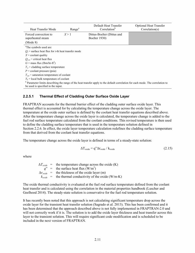
2.2.5.1 Thermal Effect of Cladding Outer Surface Oxide Layer

FRAPTRAN accounts for the thermal barrier effect of the cladding outer surface oxide layer. This thermal effect is accounted for by calculating the temperature change across the oxide layer. The temperature at the oxide outer surface is defined by the coolant heat transfer equations described above. After the temperature change across the oxide layer is calculated, the temperature change is added to the fuel rod surface temperature calculated from the coolant conditions. This revised temperature is then used to define the cladding surface temperature that is used in the temperature solution defined in Section 2.2.6. In effect, the oxide layer temperature calculation redefines the cladding surface temperature from that derived from the coolant heat transfer equations.

The temperature change across the oxide layer is defined in terms of a steady-state solution:

ΔToxide = q”Δroxide / koxide (2.15) where ΔToxide = the temperature change across the oxide (K) q” = the surface heat flux (W/m2) Δroxide = the thickness of the oxide layer (m) koxide = the thermal conductivity of the oxide (W/m-K)

The oxide thermal conductivity is evaluated at the fuel rod surface temperature defined from the coolant heat transfer and is calculated using the correlation in the material properties handbook (Luscher and Geelhood 2014). The steady-state solution is conservative for the fuel rod temperature solution.

It has recently been noted that this approach is not calculating significant temperature drop across the oxide layer for the transient heat transfer solution (Sagrado et al. 2013). This has been confirmed and it has been determined that the approach described above is not fully implemented in FRAPTRAN-2.0 and will not correctly work if it is. The solution is to add the oxide layer thickness and heat transfer across this layer to the transient solution. This will require significant code modification and is scheduled to be included in the next version of FRAPTRAN.

2.12

2.2.6 Heat Conduction and Temperature Solution

Once values for the heat generation, gap conductance, and cladding surface temperature have been obtained, the complete temperature distribution in the fuel and cladding is obtained by applying the law for heat conduction in solids in one dimension.

2.2.6.1 One-Dimensional Radial Heat Conduction

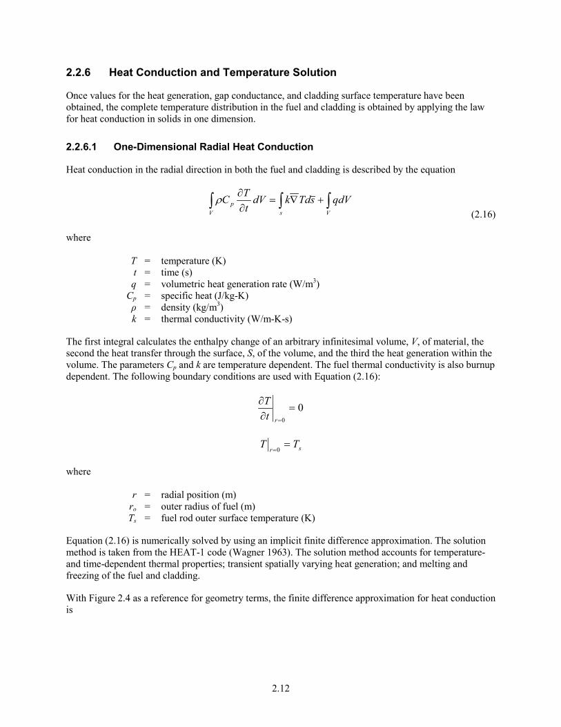
Heat conduction in the radial direction in both the fuel and cladding is described by the equation

∫∫∫ +∇=

∂∂

VsVp qdVsTdkdV

tTCρ

(2.16) where T = temperature (K) t = time (s) q = volumetric heat generation rate (W/m3) Cp = specific heat (J/kg-K) ρ = density (kg/m3) k = thermal conductivity (W/m-K-s)

The first integral calculates the enthalpy change of an arbitrary infinitesimal volume, V, of material, the second the heat transfer through the surface, S, of the volume, and the third the heat generation within the volume. The parameters Cp and k are temperature dependent. The fuel thermal conductivity is also burnup dependent. The following boundary conditions are used with Equation (2.16):

0

0

=∂∂

=rtT

srTT =

=0 where r = radial position (m) ro = outer radius of fuel (m) Ts = fuel rod outer surface temperature (K)

Equation (2.16) is numerically solved by using an implicit finite difference approximation. The solution method is taken from the HEAT-1 code (Wagner 1963). The solution method accounts for temperature- and time-dependent thermal properties; transient spatially varying heat generation; and melting and freezing of the fuel and cladding.

With Figure 2.4 as a reference for geometry terms, the finite difference approximation for heat conduction is

2.13

( )( ) ( )( ) V

rnrnVS

rnrnm

nm

n

Smn

mn

Vrnrn

Vmn

mn

hQhQhkTT

hkTTt

hchcTT

++−+

−−=∆

+−

+++

+−

++

lnln1

lnln1lnln

1

21

21

21

21

(2.17) where Tn

m+1 = temperature at radial node n and time point m+1 (K) Tn

m+1/2 = 0.5 (Tnm + Tn

m+1) Δt = time step (s) cln = volumetric heat capacity on left side of node n (J/m3⋅K) crn = volumetric heat capacity on right side of node n (J/m3⋅K) krn = thermal conductivity at right side of node n (W/m⋅K) kln = thermal conductivity at left side of node n (W/m⋅K) hln

v = volume weight of mesh spacing on left side of radial node n (m2)

=

∆

−∆4

lnln

rrr nπ

hrnv = volume weight on right side of node n (m2)

=

∆

−∆4

lnln

rrr nπ

hlns = surface weight on left side of node n

=

∆

−∆ 22 ln

ln

rrr nπ

hrns = surface weight on right side of node n

=

∆

+∆ 22 rn

nrn

rr

rπ

Qln = heat generation per unit volume for mesh spacing on left side of radial node n (W/m3)

2.14

Figure 2.4. Description of Geometry Terms in Finite Difference Equations for Heat Conduction

If a phase change from solid to liquid, or liquid to solid, occurs at radial node n, Equation (2.17) is modified to account for the storage or release of the heat of fusion while the temperature remains equal to the melting temperature. The modified equation is

Vrn

mrn

VmsrnrnL

mn

smnL

mnv

rnv

hQhQhkTT

hkTTdt

dhhH

21

21

21

21

21

lnln1

lnln1ln

)(

)()(

++++

+−

+

++−+

−−=+αρ

(2.18) where

dt

d mn

21+α

= rate of change of volume fraction of material melted in the two half mesh spacings

on either side of radial node n during the midpoint of the time step (s-1) H = heat of fusion of the material (J/kg) TL = melting temperature of the material (K)

The phase change from solid to liquid is complete when

∑=

+

=∆2

1

21

1M

Mm

mmn t

dtdα

where M1 = number of time step at which melting started M2 = number of time step at which melting ends Δtm = size of m-th time step (s)

2.15

The finite difference approximations at each radial node are combined together to form one tri-diagonal matrix equation. The equation has the form

N

Nm

N

mN

m

m

m

NN

NNN

dd

ddd

TT

TTT

bacbas

cbascba

cb

1

3

2

1

1

11

13

12

11

111

333

222

11

0'0

'0000

−+

+−

+

+

+

−−−

⋅⋅⋅

=

⋅⋅⋅

⋅

⋅⋅⋅⋅⋅⋅⋅⋅

(2.19)

Equation (2.19) is solved by Gaussian elimination for the radial node temperatures. Because the off-diagonal elements are negative and the sum of the diagonal elements is greater than the sum of the off-diagonal elements, little roundoff error occurs as a result of using Gaussian elimination.

When the forward reduction step of Gaussian elimination has been applied to Equation (2.20), the last equation in the transformed equation is:

11 ++ =+ mN

mN qBAT (2.20)

where 1+m

NT = cladding surface temperature (K)

1+mNq = cladding surface heat flux (W/m2)

A, B = coefficients that are defined in Appendix C

Equation (2.20) is combined with the correlation for convective heat transfer to solve for the cladding surface temperature, as previously shown in Figure 2.3.

The description of the calculations for the temperature distribution in the fuel and cladding is complete at this point. The calculation of the temperature of the gas in the fuel rod plenum is then needed to complete the solution for the fuel rod temperature distribution. This calculation is performed by a separate model and is described in Section 2.3.

2.2.6.2 Decay Heat Model

In addition to specifying the power history in the input file, the user may choose to account for decay heat. If the decay heat history is known in advance, it may be input manually as part of the power history. If it is not known, the ANS standard decay heat model (Scatena and Upham 1973) may be specified.

The decay heat model in FRAPTRAN-2.0 is given by the following equation:

11 )( 022b

sa

sans ttbtaf +−= (2.21)

2.16

where fans = fraction of steady state power (fraction) where the steady state power is the power

specified at time = 0 ts = time from shutdown (s) t0 = time of operation (s) a1 = - 0.0639, ts ≤ 10s - 0.181, ts > 10 s a2 = 0.0603, ts ≤ 10s 0.0766, ts > 10 s b1 = - 0.13, ts+t0 ≤ 4×106s - 0.335, ts+t0 > 4×106s b2 = 0.283, ts+t0 ≤ 4×106s 0.266, ts+t0 > 4×106s

FRAPTRAN-2.0 applies this model using the following input variables: powop: steady state power level that fans in Equation (2.21) is multiplied by timop: t0 in Equation (2.21) fpdcay: multiplicative factor on fans tpowf: time at which fpdcay is applied

ts in Equation (2.21) is set as the time within FRAPTRAN-2.0.

2.2.6.3 Stored Energy

The stored energy in the fuel rod is calculated separately for the fuel and the cladding. The stored energy is calculated by summing the energy of each pellet or cladding ring calculated at the ring temperature. The expression for stored energy is

m

dTTCm

E

I

i

T

Tpi

s

i

ref

∑ ∫=

=1

)(

(2.22)

where Es = stored energy (J/kg) mi = mass of ring segment i (kg) Ti = temperature of ring segment i (K) Tref = reference temperature for stored energy (K) Cp(T) = specific heat evaluated at temperature T for fuel or cladding (J/kg-K) m = total mass of the axial node (kg) I = number of annular rings

The stored energy in the fuel and cladding is calculated for each axial node. By default, the reference temperature, Tref, is 298K (77°F); however, this can be changed using the input file.

2.17

2.3 Plenum Gas Temperature Model

To calculate the internal fuel rod pressure, the temperature for all gas volumes in the fuel rod must be calculated. Under steady-state and transient reactor conditions, approximately 40 to 50 percent of the gas in a fuel rod is located in the fuel rod plenum provided at the top, and sometimes the bottom, of the fuel rod. Two options are available to define the temperature of the gas in the plenum. The default is to assume the gas temperature to be 10°F (5.6K) higher than the axial local coolant temperature. A more detailed model to calculate the temperature is available as a user option; the model includes all thermal interactions between the plenum gas and the top pellet surface, hold-down spring, and cladding wall.

The transient plenum temperature model is based on three assumptions:

1. The temperature of the top surface of the fuel stack is independent of the plenum gas temperature.

2. The plenum gas is well mixed by natural convection.

3. Axial temperature gradients in the spring and cladding are small.

The first assumption allows the end-pellet temperature to be treated as an independent variable. The second assumption permits the gas to be modeled as one lumped mass with average properties. The third assumption allows the temperature response of the cladding and spring to be represented by a small number of lumped masses.

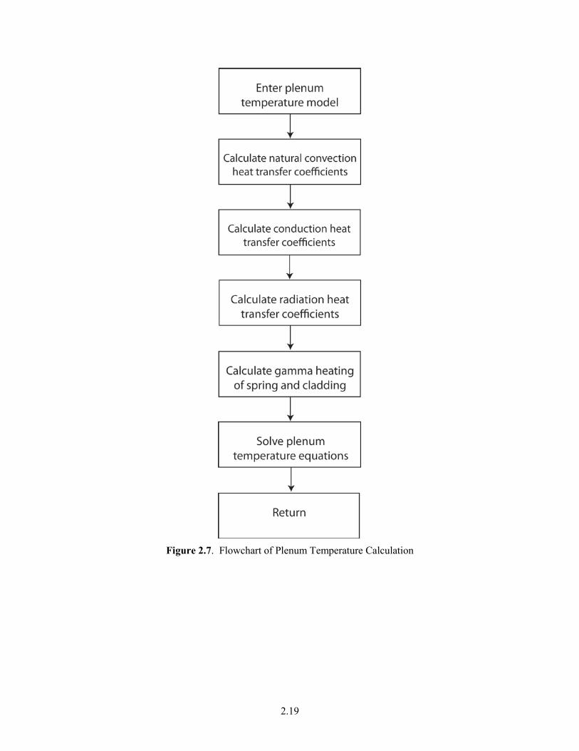
The plenum temperature model consists of a set of six simultaneous, first-order differential equations that model the heat transfer between the plenum gas and the structural components of the plenum. These equations involve heat transfer coefficients between the components. The heat transfer equations for the plenum temperature are described in Section 2.3.1. The required heat transfer coefficients are described in Section 2.3.2. Finally, the calculation of the gamma heating of the plenum hold-down spring and cladding is described in Section 2.3.3. A flowchart of the calculation is shown in Figure 2.7.

2.3.1 Plenum Temperature Equations

The plenum thermal model calculates the energy exchange between the plenum gas and structural components. The structural components consist of the hold-down spring, end pellet, and cladding. Energy exchange between the gas and structural components occurs by natural convection, conduction, and radiation. A schematic of these energy exchange mechanisms is shown in Figure 2.6. The spring is modeled by two nodes of equal mass (a center node and a surface node) as shown in Figure 2.5. The cladding is modeled by three nodes (two surface nodes and one center node) as shown in Figure 2.8. The center node has twice the mass of the surface nodes. This nodalization scheme results in a set of six energy equations from which the plenum thermal response can be calculated. The transient energy equations for the gas, spring, and cladding are as follows (the nomenclature used in the equations is defined in Table 2.2):

Figure 2.5. Energy Flow in Plenum Model – Spring Model with Two Nodes

2.18

Figure 2.6. Energy Flow in Plenum Model – Energy Exchange Mechanisms

2.19

Figure 2.7. Flowchart of Plenum Temperature Calculation

2.20

Figure 2.8. Cladding Noding

1. Plenum gas

)()()( gSSSSSgcliclclgepepep

gggg TThATThATThA

tT

CV −+−+−=∂

∂ρ

(2.23)

2. Spring center node

SS

SCSSSSCsc

SSsssc R

TTKAVq

tT

CV)( −

+=∂

∂ρ (2.24)

3. Spring surface node

)()(

)()(

SScliconsSSSSgsSS

SScliradsSSSSSCSSCSSSS

SSSS

TThATThA

TThATTKAVqt

TCV

−+−+

−+−+=∂

∂ρ

(2.25)

where hcons is the conductance between the spring and cladding.

The conductance, hcons, is used only when a stagnant gas condition exists, that is, when the natural convection heat transfer coefficient for the spring (hs) is zero.

2.21

4. Cladding interior node

clicliclcclcl

cliSSconccl

cligclclcliSSradcclcli

cliclcl

VqTTrKATThA

TThATThAt

TVC

+−∆

+−+

−+−=∂

∂

)(2/

)(

)()(ρ (2.26)

5. Cladding central node

)(2/

)(2/ clcclo

clclclccli

clclclc

clcclcclcl TT

rKA

TTrKA

Vqt

TVC −

∆+−

∆+=

∂∂

ρ (2.27)

Table 2.2. Nomenclature for Plenum Thermal Model

Quantities Subscripts A = surface area cl = cladding C = heat capacitance clc = cladding center node DIAC = diameter of the spring coil cli = cladding interior node DIAS = diameter of the spring wire clo = cladding outside node

21−F = gray-body shape factor from body 1 to body 2 cool = coolant

F1-2 = view factor from body 1 to body2 conc, cons = conduction between the spring and cladding

Gr = Grashof number conv = convective heat transfer to coolant h = surface heat transfer coefficient ep = end pellet I = gamma flux g = gas ID = inside diameter of the cladding p = plenum K = thermal conductivity sc = spring center node L = length ss = spring surface node OD = outside diameter of the cladding s = spring Pr = Prandtl number rads, radc = radiation heat transfer between the

spring and the cladding q = energy m, m+1 = old and new time step

q ′′ = surface heat flux

q ′′′ = volumetric heat generation

R = radius ∆r = thickness of the cladding: (OD-ID)/2 T = temperature V = volume σ = Stefan-Boltzmann constant Cg = heat capacitance of gas, set equal to the value of 5.188x103 J/kg-K, which is the heat capacitance of

2.22

Quantities Subscripts helium ρ = density

Σγ = absorption coefficient

ε = emissivity

δ = spring to cladding spacing: (ID-DIAC)/2 t = time

6. Cladding exterior node

coolclo TT = (2.28)

For steady-state analysis, the time derivatives of temperature on the left side of Equations (2.23) through (2.27) are set equal to zero and the temperature distribution in the spring and cladding is assumed to be uniform.

To obtain a set of algebraic equations, Equations (2.23) through (2.28) are written in the Crank-Nicolson (Crank and Nicolson 1974) implicit finite difference form. This formulation results in a set of six equations and six unknowns.

The details of the finite difference formulation of Equations (2.23) through (2.28) and the logic of the plenum temperature model are given in Appendix E.

2.3.2 Heat Conduction Coefficients

Heat transfer between the plenum gas and the structural components occurs by natural convection, conduction, and radiation. The required heat transfer coefficients for these three modes are described in the following.

2.3.2.1 Natural Convection Heat Transfer Coefficients

Energy exchange by natural convection occurs between the plenum gas and the top of the fuel pellet stack, the spring, and the cladding. Heat transfer coefficients hep, hs, and hcl, in the equations above, model this energy exchange. To calculate these heat transfer coefficients, the top of the fuel stack is assumed to be a flat plate, the spring is assumed to be a horizontal cylinder, and the cladding is assumed to be a vertical surface. Both laminar and turbulent natural convection are assumed to occur. Correlations for the heat transfer coefficients for these types of heat transfer are obtained from Kreith (1964) and McAdams (1954).

The flat plate natural convection coefficients used for the end pellet surface heat transfer are given below.

1. For laminar conditions on a heated surface

( )

IDGrKh gep

25.0Pr54.0 ×= (2.29)

2. For turbulent conditions (Grashof Number [Gr] greater than 2.0x107) on a heated surface

2.23

( )

IDGrKh gep

33.0Pr14.0 ×= (2.30)

3. For laminar conditions on a cooled surface

( )

IDGrKh gep

25.0Pr27.0 ×= (2.31)

The following natural convection coefficients for horizontal cylinders are used for the film coefficient for the spring.

1. For laminar conditions

( )

DIASGrKh gs

25.0Pr53.0 ×= (2.32)

2. For turbulent conditions (Gr from 1×109 to 1×1012)

( ) 33.018.0 SSgs TTh −= (2.33)

The vertical surface natural convection coefficients used for the cladding interior surface are given below.

1. For laminar conditions

( )

pgcl L

GrKh25.0Pr55.0 ×

= (2.34)

2. For turbulent conditions (Gr greater than 1×109)

( )

pgcl L

GrKh4.0Pr021.0 ×

= (2.35)

These natural convection correlations were derived for flat plates, horizontal cylinders, and vertical surfaces in an infinite gas volume. Heat transfer coefficients calculated using these correlations are expected to be higher than those actually existing within the confined space of the plenum. However, until plenum temperature experimental data are available, these coefficients are believed to provide an acceptable estimate of the true values.

2.3.2.2 Conduction Heat Transfer Coefficients

Conduction of energy between the spring and cladding is represented by the heat transfer coefficients hcons and hconc in Equations (2.25) and (2.26). These coefficients are both calculated when stagnant gas conditions exist. The conduction coefficients are calculated based on the spring and cladding geometries shown in Figure 2.9 and the following assumptions:

1. The cladding and spring surface temperatures are uniform.

2.24

2. Energy is conducted only in the direction perpendicular to the cladding wall (heat flow is one-dimensional).

Based on these assumptions, and the geometry given in Figure 2.9, the energy (q) conducted from an elemental surface area of the spring (LsRsdθ) to the cladding is

)sin(

))sin()((θ

θθ

SS

SScliSSg

RRddRLTTK

dq−+

−= (2.36)

where θ is the azimuthal coordinate.

By integration of Equation (2.36) over the surface area of the spring facing the cladding, the total flow of energy is given by

2

0

2

21

2

2

)2(1

)2(2tan

tan)2(

11

22

)(

πθ

θδ

δθ

δπ

π

=

=

−

+−

+−

++−

+−−=

S

S

S

S

S

S

SScliSS

SSg

RR

RR

RR

RRTT

Akq (2.37)

The two conduction heat transfer coefficients are given by

hcons = q/Ass (Tss - Tcli) and

hconc = hcons Ass/Acl

When natural convection heat transfer exists (hcl or hs greater than 0.0), energy is assumed to flow to the gas from the spring and then from the gas to the cladding wall, or vice versa. Under these conditions, hcons and hconc are set equal to zero. Therefore, hcons and hconc are used only when the temperature is uniform throughout the plenum. Future plenum data or analytical analysis may indicate that natural convection flow between the spring and cladding does not exist, in which case non-zero conduction coefficients will be used at all times.

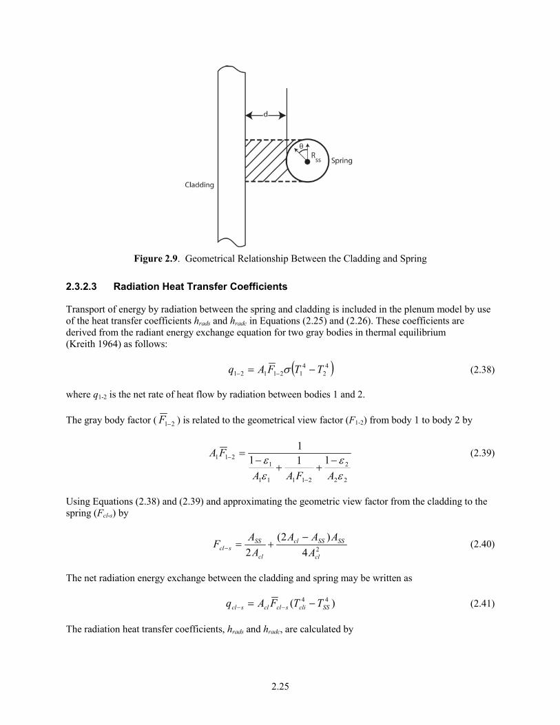
2.25

Figure 2.9. Geometrical Relationship Between the Cladding and Spring

2.3.2.3 Radiation Heat Transfer Coefficients

Transport of energy by radiation between the spring and cladding is included in the plenum model by use of the heat transfer coefficients hrads and hradc in Equations (2.25) and (2.26). These coefficients are derived from the radiant energy exchange equation for two gray bodies in thermal equilibrium (Kreith 1964) as follows:

( )42

4121121 TTFAq −= −− σ (2.38)

where q1-2 is the net rate of heat flow by radiation between bodies 1 and 2.

The gray body factor ( 21−F ) is related to the geometrical view factor (F1-2) from body 1 to body 2 by

22

2

21111

1211 111

1

εε

εε

AFAA

FA−

++−

=

−

− (2.39)

Using Equations (2.38) and (2.39) and approximating the geometric view factor from the cladding to the spring (Fcl-s) by

24)2(

2 cl

SSSScl

cl

SSscl A

AAAA

AF

−+=− (2.40)

The net radiation energy exchange between the cladding and spring may be written as

)( 44SSclisclclscl TTFAq −= −− (2.41)

The radiation heat transfer coefficients, hrads and hradc, are calculated by

2.26

( )SSclicl

sclradc TT

Aq

h −= − (2.42)

and

SS

clradcrads A

Ahh = (2.43)

2.3.2.4 Gamma Heating of the Spring and Cladding

The volumetric power generation term, q, used in Equations (2.24) through (2.27), represents the gamma radiation heating of the spring and cladding. A simple relationship is used to calculate q. The relationship used is derived from the gamma flux attenuation equation:

dxxIxdI )()( γΣ=− (2.44) where I(x) = gamma flux Σγ = gamma ray absorption coefficient x = spatial dimension of solid on which the gamma radiation is incident

Because the cladding and spring are thin in cross-section, the gamma ray flux can be assumed constant throughout the volume. Of the gamma flux, I, incident on the spring and cladding, the portion absorbed, ΔI, can be described by

xII γΣ=∆− (2.45)

where x is the thickness of the spring or cladding. Therefore, the volumetric gamma ray absorption rate is given by

IxI

γΣ=∆

− (2.46)

Equation (2.46) can also represent gamma volumetric energy deposition by letting I represent the energy flux associated with the gamma radiation. Approximately 10 percent of the energy released in the fissioning of uranium is in the form of high-energy gamma radiation. Therefore, the gamma energy flux leaving the fuel rod would be approximately equal to 10 percent of the thermal flux. The gamma energy flux throughout the reactor can then be estimated by

rodqI 10.0= (2.47)

where rodq is the average fuel rod power (kW/m). For zirconium, Σγ is approximately 36.1 m-1. Therefore, the gamma energy deposition rate is given by

rodqqxI 61.3==

∆− (2.48)

2.27

Equation (2.48) is an estimate of the gamma heating rate for the spring and cladding.

2.4 Fuel Rod Mechanical Response Model

An accurate analysis of the fuel and cladding mechanical response is necessary in any fuel rod response analysis because the heat transfer across the fuel-cladding gap is a strong function of the gap size. In addition, an accurate calculation of stresses in the cladding is needed so that an accurate prediction of the extent of cladding ballooning and failure (and subsequent release of fission products) can be made. The two cladding failure models in FRAPTRAN are discussed in Section 2.8.

In analyzing the mechanical response of fuel rods, two physical situations are encountered. The first situation occurs when the fuel pellets and cladding are not in contact. Here, the problem of a cylindrical shell (the cladding) with specified internal and external pressures and a specified cladding temperature distribution must be solved. This situation is called the “open gap” regime.

The second situation encountered is when the fuel pellets come into contact with the cladding. This will occur as a combination of differential thermal expansion between the fuel and cladding, fission-product induced swelling of the fuel, and creep-down of the cladding. This situation is called the “closed gap” regime and results in fuel pellet/cladding mechanical interaction (PCMI).

The mechanical model used in FRAPTRAN for calculating the mechanical response of the fuel and cladding is the FRACAS-I model; this model is also used in FRAPCON. This model does not account for stress-induced deformation of the fuel and therefore is called the rigid pellet model. This model includes the effects of thermal expansion of the fuel pellet; rod internal gas pressure; and thermal expansion, plasticity, and high-temperature creep of the cladding.

After the cladding strain has been calculated by the mechanical model, the strain is compared with the value of an instability strain obtained from MATPRO (Hagrman et al. 1981). If the instability strain has been exceeded at any point along the rod, then the cladding cannot maintain a cylindrical shape and local ballooning occurs. For the local region at which instability is predicted, a large deformation ballooning analysis is performed. No further strain is calculated for non-ballooning nodes. Modification of local heat transfer coefficients is calculated as the cladding ballooning progresses and additional surface area is presented to the coolant.

In Section 2.4.1, the general theory of plastic analysis is outlined. In Section 2.4.2, the theory is extended to include creep and hot pressing. In Section 2.4.3, the equations for the FRACAS-I model are described. In Section 2.4.4, the model for local cladding ballooning is summarized.

2.4.1 General Considerations in Elastic-Plastic Analysis

Problems involving elastic-plastic deformation and multiaxial states of stress involve aspects that do not require consideration in a uniaxial problem. In the following discussion, an attempt is made to briefly outline the structure of incremental plasticity and to outline the method of successive substitutions (also called method of successive elastic solutions), which has been used successfully in treating multiaxial elastic-plastic problems (Mendelson 1968). The method can be used for any problem for which a solution based on elasticity can be obtained. This method is used in the rigid pellet model.

In a problem involving only uniaxial stress, σ1, the strain, ε1, is related to the stress by an experimentally determined stress-strain curve, as shown in Figure 2.10, and Hooke’s law, which is taken as

2.28

∫++= dTE

P αεσ

ε 11

1 (2.49)

where P1ε is the plastic strain and E is the modulus of elasticity. The onset of yielding occurs at the yield

stress, which can be determined directly from Figure 2.10. Given a load (stress) history, the resulting deformation can be determined in a simple fashion. Increase of the yield stress with work-hardening is easily calculated directly from Figure 2.10.

In a problem involving multiaxial states of stress, however, the situation is not so clear. In such a problem, a method of relating the onset of plastic deformation to the results of a uniaxial test is required. Furthermore, when plastic deformation occurs, some means is needed for determining how much plastic deformation has occurred and how that deformation is distributed among the individual components of strain. These two complications are taken into account by use of the so-called “yield function” and “flow rule,” respectively.

A substantial quantity of experimental evidence exists on the onset of yielding in a multiaxial stress state. Most of this evidence supports the von Mises yield criterion (Murphy 1946), which asserts that yielding occurs when the stress state is such that

( ) ( ) ( )( ) 2213

232

2215.0 yσσσσσσσ =−+−+− (2.50)

where the σi (i=1, 2, 3) values are the principal stresses and σy is the yield stress as determined in a uniaxial stress-strain test. The square root of the left side of Equation 2.50 is referred to as the “effective stress,” σe, and this effective stress is one commonly used type of yield function.

To determine how the yield stress changes with permanent deformation, the yield stress is hypothesized to be a function of the equivalent plastic strain, εp. An increment of equivalent plastic strain is determined at each load step, and εp is defined as the sum of all increments incurred, as follows:

∑∆

= pp dεε (2.51)

2.29

Figure 2.10. Typical Isothermal True Stress-strain Curve

Each increment of effective plastic strain is related to the individual plastic strain components by

212

132

322

21 ])()()[(32 ppppppp ddddddd εεεεεεε −+−+−= (2.52)

where the Pidε (i = 1, 2, and 3) are the plastic strain components in principle coordinates. Well known

experimental results indicate that at pressures on the order of the yield stress, plastic deformation occurs with no change in volume. This implies that

0321 =++ ppp ddd εεε (2.53)

In a uniaxial test with σ1 = σ and σ2 = σ3 = 0, the plastic strain increments are

ppp ddd 121

32 εεε −== (2.54)

Hence, in a uniaxial test, Equations (2.50) and (2.52) reduce to

1σσ =e

pp dd 1εε = (2.55)

Thus, when the assumption is made that the yield stress is a function of the total effective plastic strain (called the strain hardening hypothesis [Mendelson 1968]), the functional relationship between yield stress and plastic strain can be taken directly from a uniaxial stress-strain curve by virtue of Equation (2.55).

2.30

The relationship between the magnitudes of the plastic strain increments and the effective plastic strain increment is provided by the Prandtl-Reuss flow rule (Prandtl 1924):

ie

pp

i Sddσεε

23

+ i = 1, 2, 3 (2.56)

where the Si values are the deviatoric stress components (in principal coordinates) defined by

)( 32131 σσσσ ++−= iiS i = 1, 2, 3 (2.57)

Equation (2.56) embodies the fundamental observation of plastic deformation; that is, plastic strain increments are proportional to the deviatoric stresses. The constant of proportionality is determined by the choice of the yield function (Mendelson 1968). Direct substitution shows that Equations (2.50), (2.51), (2.52), (2.56), and (2.57) are consistent with one another.

Once the plastic strain increments have been determined for a given load step, the total strains are determined from a generalized form of Hooke’s law, given by

∫++++−= dTdE

pp1113211 )}({1 αεεσσνσε

∫++++−= dTdE

pp2223122 )}({1 αεεσσνσε (2.58)

∫++++−= dTdE

pp3331233 )}({1 αεεσσνσε

in which p1ε , p

2ε , and p3ε are the total plastic strain components at the end of the previous load

increment.

The remaining continuum field equations of equilibrium, strain displacement, and strain compatibility are unchanged. The complete set of governing equations is presented in Table 2.3; these equations are written in terms of rectangular Cartesian coordinates and employ the usual indicial notation in which a repeated Latin index implies summation. This set of equations is augmented by an experimentally determined uniaxial stress-strain relation.

When the problem under consideration is statically determinate, so that stresses can be found from equilibrium conditions alone, the resulting plastic deformation can be determined directly. However, when the problem is statically indeterminate such that the stresses and deformation must be found simultaneously, then the full set of plasticity equations proves to be quite formidable even in the case of simple loadings and geometries.

One numerical procedure which has been used with considerable success is the method of successive substitutions. This method can be applied to any problem for which an elastic solution can be obtained, either in closed form or numerically. A full discussion of this technique, including a number of technologically useful examples, is contained in Mendelson (1968).

2.31

The method involves breaking the load path into small increments. For example, in mechanical analysis of fuel rods, the loads are the coolant pressure and either fuel rod internal gas pressure or a prescribed displacement of the inside surface of the cladding due to thermal expansion of the fuel. These loads all vary during the operating history of the fuel rod. For each new increment of the loading, the solution to all the plasticity equations listed in Table 2.3 is obtained as described in the following.

First, an initial estimate of the plastic strain increment, Pijdε , is made. Based on this value, the equations

of equilibrium, Hooke’s law, and strain displacement and compatibility are solved as for any elastic problem. From the stresses so obtained, the deviatoric stresses, Sij, may be calculated. This “pseudo-elastic” solution represents one path in the computational scheme.

Independently, through use of the Pijdε values, the increment of effective plastic strain, dεp, may be

calculated. From this result and the stress-strain curve, a value of the effective stress, σe, can be obtained.

Finally, a new estimate of the plastic strain increment is obtained from the Prandtl-Reuss rule:

ije

pp

ij Sddσεε

23

= (2.59)

and the entire process is continued until the Pijdε converge. A schematic of the iteration scheme is

provided in Figure 2.11.

The mechanism by which improved estimates of Pijdε are obtained results from the fact that the effective

stress obtained from dεp and the stress-strain curve will not be equal to the effective stress that would be obtained with the stresses from the elastic solution. The effective stresses will only agree when convergence is obtained.

The question of convergence is one that cannot, in general, be answered a priori. However, convergence can be shown (Mendelson 1968) to be obtained for sufficiently small load increments. Experience has shown that this technique is suitable for both steady-state and transient fuel rod analyses.

2.32

Table 2.3. Elastic-plastic Governing Equations

Equilibrium

σji,j+ρfi= 0 where σ = stress tensor ρ= mass density fi= components of body force per unit mass

Stress strain

pij

pijkkijijij ddT

EEεεασνδσνε ++

−−

+= ∫

1

Compatibility

εij,kl + εkl,ij - εik,jl - εjl,ik = 0 Definitions used in plasticity

ijije SS23∆

=σ

kkijijS σσ31

−=∆

Pij

Pij

P ddd εεε 32=

∆

Prandtl-Reuss flow rule

ije

pp

ij Sddσεε

23

=

2.4.2 Extension to Creep and Hot Pressing

The method of solution described for the time-independent plasticity calculations can also be used for time-dependent creep and hot pressing calculations. In this context, the term “creep” refers to any time-dependent constant volume permanent deformation; whereas the term “hot pressing” refers to any time-dependent process which results in a permanent change in volume. Both creep and hot pressing are stress-driven processes and are usually highly dependent on temperature.

The only change required to extend the method of successive substitutions to allow consideration of creep and hot pressing is to rewrite the Prandtl-Reuss flow rule, Equation (2.56), as follows.

2.33

Figure 2.11. Schematic of the Method of Successive Elastic Solutions

( )

m

c

e

cc tVStd

σσσσ

σεε 321

11 95.1

++∆+

∆=

( )

m

c

e

cc tVStd

σσσσ

σεε 321

22 95.1 ++∆

+∆

=

(2.60)

( )

m

c

e

cc tVStd

σσσσ

σεε 321

33 95.1

++∆+

∆=

where σm is the mean stress.

The first term on the right-hand side of each of these equations calculates the constant volume creep strain, whereas the second term in each equation calculates the permanent change in volume. To use this form of the flow rule, two additional material property correlations must be available. These correlations are shown in the next two sections.

2.4.2.1 Constant Volume Creep

The correlation for constant volume creep strain, εc, as a function of stress, time, temperature, and neutron flux, is assumed to be:

),,,( φσε tTfc = (2.61) where σ = uniaxial stress (MPa) T = temperature (K) t = time (s) φ = neutron flux (neutrons/m2-s)

2.34

The strain hardening hypothesis (Mendelson 1968) is assumed, which implies that the creep strain correlation can be differentiated and solved for the creep strain rate in the form

),,,( φεσε th cc = (2.62)

which is no longer an explicit function of time. This equation is obtained during the creep calculations described in the FRAPCON description document (Geelhood and Luscher 2014a).

2.4.2.2 Initial Void Volume and Fuel Relocation

The initial void volume is related to the radial displacement due to fuel relocation by the equation

[ ]22)( prpo rUrV −+= π (2.63) where rp = as-fabricated radius of fuel pellets (m) Ur = radial displacement of outer surface of fuel pellets due to relocation (m)

2.4.3 Rigid Pellet Model (FRACAS-I)

To summarize the mechanical response calculations, the code assumes that stress-induced deformation of the fuel pellets is ignored. The cladding deformation model in FRACAS-I is described in Section 2.4.3.1. The cladding mechanical properties models are described in Section 2.4.3.2. The fuel deformation model is described in Section 2.4.3.3. If the fuel-cladding gap is closed, the fuel deformation model will apply a driving force to the cladding deformation model. The cladding deformation model, however, never influences the fuel deformation model.

2.4.3.1 Cladding Deformation Model

The cladding deformation model in FRACAS-I is based on the following assumptions:

1. Incremental theory of plasticity.

2. Prandtl-Reuss flow rule.

3. Isotropic work hardening.

4. No low-temperature creep deformation of cladding.

5. Thin wall cladding (stress, strain, and temperature uniform through cladding thickness).

6. No axial slippage occurs at fuel-cladding interface when fuel and cladding are in contact.

7. Bending strains and stresses in cladding are negligible.

8. Axisymmetric loading and deformation of the cladding.

Deformation and stresses in the cladding in the open gap regime are calculated using a model which considers the cladding to be a thick cylindrical shell (stress at mid-wall) with specified internal and external pressures and a prescribed uniform temperature.

2.35

Calculations for the closed gap regime are made using a model which assumes that the cladding is a thin cylindrical shell with prescribed external pressure and a prescribed radial displacement of its inside surface. The prescribed displacement is obtained from the fuel thermal expansion model. Furthermore, because no slippage is assumed when the fuel and cladding are in contact, the axial expansion of the fuel is transmitted directly to the cladding. Hence, the change in axial strain in the shell is also prescribed.

Two additional models are used to calculate changes in yield stress with work hardening, given a uniaxial stress-strain curve. This stress-strain curve is obtained from the mechanical properties given in Section 2.4.3.2. The first model calculates the effective total strain and new effective plastic stress given a value of effective stress and the effective plastic strain at the end of the last loading increment. Depending on the work-hardened value of yield stress, loading can be either elastic or plastic, and unloading is constrained to occur elastically. (Isotropic work hardening is assumed in these calculations.)

The determination as to whether or not the fuel is in contact with the cladding is made by comparing the radial displacement of the fuel with the radial displacement that would occur in the cladding due to the prescribed external (coolant) pressure and the prescribed internal (fission and fill gas) pressure. The determination is expressed by the equation

δ+≥ cladr

fuelr uu (2.64)

where δ = as-fabricated fuel-cladding gap size (m) ur = radial displacement (m)

If the above equation is satisfied, the fuel is determined to be in contact with the cladding. The loading history enters into this determination by virtue of the permanent plastic cladding strains imposed in the cladding by the cladding loads.

If the fuel and cladding displacements are such that Equation (2.64) is not satisfied, the fuel-cladding gap has not closed during the current loading step and the open gap solution is used.

If Equation (2.63) is satisfied, however, the fuel and cladding have come into contact during the current loading increment. At the contact interface, radial continuity requires that

δ−= fuelr

cladr uu (2.65)

while in the axial direction the assumption is made that no slippage occurs between the fuel and cladding. This state is referred to as PCMI or “lockup.”

Note that only the additional strain which occurs in the fuel after PCMI has occurred is transferred to the cladding. Thus, if clad

oz ,ε is the axial strain in the cladding just prior to contact and fueloz ,ε is the

corresponding axial strain in the fuel, then the no-slippage condition in the axial direction becomes

fueloz

fuelz

cladoz

cladz ,, εεεε −=− (2.66)

After cladru and clad

zε have been calculated, a solution is made of the stresses and strains in a thin cylindrical shell with prescribed axial strain, external pressure, and prescribed radial displacement of the inside surface. The solution also gives the interface pressure between the fuel and cladding.

2.36

The open gap modeling considers a thin cylindrical shell loaded by both internal and external pressures. Axisymmetric loading and deformation are assumed. Loading is also restricted to being uniform in the axial direction, and no bending is considered. The geometry and coordinates are shown in Figure 2.12. The displacements of the midplane of the shell are u and w in the radial and axial directions, respectively.

For this case, the equilibrium equations are identically satisfied by

t

PrPr ooii −=θσ (2.67)

22

22

io

ooiiz rr

PrPr−−

=σ (2.68)

where σθ = hoop stress (N/m2) σz = axial stress (N/m2) ri = inside radius of cladding (m) ro = outside radius of cladding (m) Pi = internal pressure of fuel rod (N/m2) Po = coolant pressure (N/m2) t = cladding thickness (m)

Figure 2.12. Fuel Rod Geometry and Coordinates

From membrane shell theory (Wang 1953), the strains are related to the midplane displacements by

zw

z ∂∂

=ε (2.69)

2.37

ru

=θε (2.70)

where r is the radius of the midplane. Strain across the thickness of the shell is allowed. The radial stress is neglected. The hoop stress, σθ, and axial stress, σz, are uniform across the cladding thickness. The radial strain is due only to the Poisson effect and is uniform across the cladding thickness. (Normally, radial strains are not considered in the shell analysis, but when plastic deformations are considered, plastic radial strains must be included.)

The stress-strain relations are written in the incremental form:

∫+++−=T

T

PPz dTd

E0

}{1 αεενσσε θθθθ (2.71)

∫+++−=T

T

Pz

Pzzz dTd

E0

}{1 αεενσσε θ (2.72)

∫++++−=T

T

Pr

Przr dTd

E0

}{ αεεσσνε θ (2.73)

where To = strain-free reference temperature (K) α = coefficient of thermal expansion (K-1) T = current cladding temperature (K) E = modulus of elasticity (N/m2) ν = Poisson’s ratio

The terms Pθε , P

zε , and Prε are the plastic strains at the end of the last load increment, and Pd θε , P

zdε ,

and Prdε are the additional plastic strain increments which occur during the new load increment.

The magnitudes of the additional plastic strain increments are determined by the effective stress and the Prandtl-Reuss flow rule, which are expressed as

21

])()()[(2

1 222θθ σσσσσ ++−= zze (2.74)

ie

pp

i Sddσεε

23

= for i = r, θ, z (2.75)

)(31

ziiS σσσ θ +−= for i = r, θ, z (2.76)

2.38

The solution of the open gap case proceeds as follows. At the end of the last load increment, the plastic strain components, P

θε , Pzε , and P

rε , are known and the total effective plastic strain, εp, is also known.

The loading is now incremented with the prescribed values of Pi, Po, and T. The new stresses can be determined from Equations (2.67) and (2.68), and a new value of effective stress is obtained from Equation (2.74).

The increment of effective plastic strain, dεp, which results from the current increment of loading, can then be determined from the uniaxial stress-strain curve at the new value of σe, as shown in Figure 2.13. (The new elastic loading curve depends on the value of εp.)

Once dεp is determined, the individual plastic strain components are found from Equation (2.75), and the total strain components are obtained from Equations (2.70) through (2.73).

The displacement of the inside surface of the shell must be determined so that a new fuel-cladding gap width can be calculated. The radial displacement of the inside surface is given by

ritrru εεθ 2

)( −= (2.77)

where the first term is the radial displacement of the midplane (from Equation (2.70)) and εr is the uniform strain across the thickness.

Figure 2.13. Calculation of Increment of Plastic Strain, dε P, from Effective Stress, σe

The cladding thickness, t, is computed by the equation

2.39

t = (1 + εr) to (2.78)

where to is the as-fabricated thickness of cladding.

The final step is to add the plastic strain increments to the previous strain values, that is,

P

oldP

newP d θθθ εεε += )()( (2.79)

Pzold

Pznew

Pz dεεε += )()( (2.80)

Prold

Prnew

Pr dεεε += )()( (2.81)

Pold

Pnew

P dεεε += )()( (2.82)

Thus, all the stresses and strains can be computed directly because, in this case, the stresses are determinate. In the case of the “fuel-driven” cladding displacement, the stresses depend on the displacement, and such a straightforward solution is not possible.

The closed gap modeling considers the problem of a cylindrical shell for which the radial displacement of the inside surface and axial strain are prescribed. Here, the stresses cannot be calculated directly because the pressure at the inside surface is exerted by the fuel instead of the internal gas and must be determined as part of the solution.

As in the open gap modeling, the displacement at the cladding inside surface is given by

rituru ε2

)( −= (2.83)

where u is the radial displacement of the cladding midplane. From Equation (2.70), u = rεθ and

ritrru εεθ 2

)( −= (2.84)

Thus, prescribing the displacement of the inside surface of the shell is equivalent to a constraining relation between εθ and εr. As before, Hooke’s law is taken in the form

∫+++−=T

T

PPz dTd

E0

}{1 αεενσσε θθθθ (2.85)

∫+++−=T

T

Pz

Pzzz dTd

E0

}{1 αεενσσε θ (2.86)

∫++++−=T

T

Pr

Przr dTd

E0

}{ αεεσσνε θ (2.87)

2.40

Use of Equations (2.84) and (2.87) in Equation (2.85) results in a relation between the stresses, σθ and σz, and the prescribed displacement u(ri):

−+

+

=

++−

+++ ∫∫

z

T

T

PPT

T

Pr

Pr

i

rt

rt

E

dTddTdrr

ru

σνσν

αεεαεε

θ

θθ

122

11

21

21)(

00 (2.88)

Equations (2.86) and (2.87) are now a pair of simultaneous algebraic equations for the stresses σθ and σz, which may be written as

=

2

1

2221

1211

BB

AAAA

zσσ θ (2.89)

where

A11 = rt

21 ν

+

A12 =

−1

2rtν

A21 = - ν A22 = 1

B1 =

++−

+++ ∫∫T

T

PPT

T

Pr

Pr

i dTdEdTdr

EtrruE

002

)( αεεαεε θθ

B2 =

++− ∫

T

T

Pz

Pzz dTdEE

0

αεεε

Then the stresses can be written explicitly as

21122211

122221

AAAAABAB

−−

=θσ (2.90)

21122211

211112

AAAAABAB

z −−

=σ (2.91)

These equations relate the stresses to u(ri) and εz, which are prescribed, and to Pd θε , Pzdε , and P

rdε , which are to be determined. The remaining equations which must be satisfied are

21

])()()[(2

1 222θθ σσσσσ ++−= zze (2.92)

2.41

21222 ])()()[(

32 p

rpz

pz

pppr

p ddddddd εεεεεεε θθ −+−+−= (2.93)

and the Prandtl-Reuss flow equations (defined in Equation [2.75])

+−= )(

31

23

ze

pp dd σσσ

σεε θθθ (2.94)

+−= )(

31

23

zze

ppz

dd σσσσεε θ (2.95)

pz

ppr ddd εεε θ −−= (2.96)

The effective stress, σe, and the effective plastic strain increment, dεp, must be related by the uniaxial stress-strain law. Equations (2.90) through (2.96) must be simultaneously satisfied for each loading increment.

As discussed in Section 2.4.1, a straightforward numerical solution to these equations can be obtained using the method of successive elastic solutions. By this method, arbitrary values are initially assumed for the increments of plastic strain, and Equations (2.90) through (2.96) are used to obtain improved estimates of the plastic strain components. The steps performed are as follows for each increment of load.

1. Values of Pd θε , Pzdε , and P

rdε are assumed. Then, dεp is calculated from Equation (2.93) and the effective stress is obtained from the stress-strain curve with strain at the value of εp.

2. From Hooke’s law, still using the assumed plastic strain increments and the prescribed values of u(ri) and εz, values for the stresses can be obtained from Equations (2.90) and (2.91).

3. New values for Pd θε , Pzdε , and P

rdε are now calculated from the Prandtl-Reuss relations, using σe

as computed in Step 1 and σθ and σz as computed in Step 2.

+−= )(

31

23

zie

pp

idd σσσσεε θ for i = r, θ, z (2.97)

4. The old and new values of Pd θε , Pzdε , and P

rdε are compared and the process continues until convergence is obtained.

5. Once convergence has been obtained, the fuel-cladding interfacial pressure is computed from Equation (2.67) as follows:

i

oo

rPrt

P+

= θσint (2.98)

When steps 1 through 5 have been completed, the solution is complete, provided that the fuel-cladding interface pressure is not less than the local gas pressure. However, due to unequal amounts of plastic straining in the hoop and axial directions upon unloading, the fuel-cladding interfacial pressure, as

2.42

obtained in step 5, is often less than the internal gas pressure, even though the fuel-cladding gap has not opened. When this occurs, the frictional “locking” mechanism (which is assumed to constrain the cladding axial deformation to equal the fuel axial deformation) can no longer act. The axial strain and stress adjust themselves so that the fuel-cladding interfacial pressure just equals the gas pressure, at which point the axial strain is again “locked.” Thus, upon further unloading, the axial strain and the hoop and axial stresses continually adjust themselves to maintain the fuel-cladding interfacial pressure equal to the gas pressure until the fuel-cladding gap is open. Because the unloading occurs elastically, a solution for this portion of the fuel-cladding interaction problem can be obtained directly, as discussed below.

Because the external pressure and the fuel-cladding interfacial pressure are known, the hoop stress is obtained from Equation (2.67) as

t

PrPr ooi −= int

θσ (2.99)

From Equation (2.84), the following expression can be written:

r

u rtfuel

r εδεθ

2+−= (2.100)

Substitution of εθ and εr, as given by Equations (2.85) and (2.86), into Equation (2.100) results in an explicit equation for σz:

( ) ( ) )(2

)( 2 iPr

Ptzi rEuddTEtddTErrr −+−+++= ∫∫ εαεασνσν θθ (2.101)

in which σθ is known from Equation (2.99). With σz and σθ known, the strains may be computed from Hooke’s law, Equations (2.85) through (2.87). This set of equations is automatically invoked whenever Pint is calculated to be less than the local internal gas pressure.

Both the closed and open gap models require the relation of stress to strain, taking into consideration the direction of loading and the previous plastic deformation. A typical stress-strain curve is shown in Figure 2.14. This curve represents the results of a uniaxial stress-strain experiment and may be interpreted (beyond initial yield) as the locus of work-hardened yield stress. The equation of the curve is provided in Section 2.4.3.2 for a wide range of temperatures.

To use this information, the usual idealization of the mechanical behavior of metals is made. Thus, linear elastic behavior is assumed until a sharply defined yield stress is reached, after which plastic (irrecoverable) deformation occurs. Unloading from a state of stress beyond the initial yield stress, o

yσ , is assumed to occur along a straight line having the elastic modulus for its slope. When the (uniaxial) stress is removed completely, a residual plastic strain remains, and this completely determines the subsequent yield stress. That is, when the specimen is loaded again, loading will occur along line BA in Figure 2.14 and no additional plastic deformation will occur until point A is again reached. Point A is the subsequent yield stress. If σ = f(ε) is the equation of the plastic portion of the stress=strain curve (YAC), then for a given value of plastic strain, the subsequent yield stress is found by simultaneously solving the following pair of equations.

2.43

Figure 2.14. True Stress-strain Curve and Unloading Path

)(

)(PE

fεεσ

εσ−=

= (2.102)

which may be written as

+= P

Ef εσσ (2.103)

The solution to this nonlinear equation may be found very efficiently by Newton’s iteration scheme:

+=+ P

mm

Ef εσσ 1 m = 0, 1, 2,… (2.104)

The initial iterate, σ(0), is arbitrary and, without loss of generality, is taken as 34.5 MPa. For any monotonically increasing stress-plastic strain relation, the iteration scheme in Equation (2.104) can be proven to converge uniformly and absolutely.

To compute the new value of the total strain, ε, and the increment of plastic strain, dεp, the following steps are performed.

1. For the given temperature, the σ = f(ε) relation is obtained from the equations in Section 2.4.3.2.

2. The yield stress, σy, for the old εp is calculated from Equation (2.104).

3. The value of the increment of plastic strain is calculated from the equations

2.44

if σ ≤ σy, P

Eεσε += (2.105)

Pold

Pnew εε = (2.106)

if σ > σy, )(σε f= (2.107)

E

Pnew

σεε −= (2.108)

Pold

Pnew

Pd εεε −= (2.109)

To compute the new value of stress, σ, given the temperature, old value of effective plastic strain, and increment of plastic strain, dεp, the following steps are performed.

1. For the given temperature, the σ = f(ε) relation is obtained from the equations in Section 2.4.3.2.

2. The yield stress, σy, for given εp, is calculated from Equation (2.104).

3. Given dεp (see Figure 2.15):

Because dεp > 0, the new values of stress and strain must lie on the plastic portion of the stress-strain curve, σ = f(ε). Therefore, σ and ε are obtained by simultaneously solving, as before,

)(

)(PnewE

fεεσεσ

−==

(2.110)

PPold

Pnew dεεε += (2.111)

2.45

Figure 2.15. Computing Stress

2.4.3.2 Cladding Mechanical Properties Models

The mechanical properties of fuel rod Zircaloy cladding are known to change with irradiation because of damage from the fast neutron fluence. The changes are similar to cold-working the material because dislocation tangles are created that tend to both strengthen and harden the cladding while decreasing the ductility. In addition to the fast fluence effects, excess hydrogen in the Zircaloy, in the form of hydrides, may affect the mechanical properties.

An analysis of recent data from mechanical testing of irradiated Zircaloy was conducted as part of the development work for FRAPCON and revised equations for use in FRAPCON and FRAPTRAN routines were then generated (Geelhood et al. 2008). The following summarizes the mechanical property equations.

Three models account for the high fast neutron fluence levels, temperature, and strain rate in the cladding. Those models are a) the strength coefficient in CKMN, b) the strain hardening exponent in CKMN, and c) the strain rate exponent in CKMN.

Strength Coefficient, K

The strength coefficient, K, is a function of temperature, fast neutron fluence, cold work, and alloy composition. The strength coefficient has not been found to be a function of hydrogen concentration. The models for the strength coefficients of Zircaloy-2 and Zircaloy-4 are given below.

2.46

)(/))()(1()( ZryKKCWKTKK Φ++⋅= (2.112) where K = strength coefficient (Pa)

32359 72752.11028185.31054859.41017628.1)( TTTTK ⋅+×−×+×= T <

750K

××= 2

66 108500027.2exp10522488.2)(

TTK

750K < T < 1090K

TTK 58 104345448.110841376039.1)( ×−×= 1090K < T < 1255K

332147 1033.7107579.310685.610330.4)( TTTTK −×−×+×−×= 1255K < T <

2100K

CWCWK ⋅= 546.0)( ),()10464.11464.0()( 25 TCWfK Φ×+−=Φ −

Φ < 0.1×1025 n/m²

Φ×=Φ −2610928.2)(K 0.1×1025n/m² < Φ < 2×1025 n/m²

Φ×+=Φ −27106618.253236.0)(K 2×1025 n/m² < Φ < 12×1025 n/m²

1

10550exp,1min)20exp(25.2),( +

−

⋅⋅−=TCWTCWf

K(Zry) =1 for Zircaloy-4 K(Zry) =1.305 for Zircaloy-2 T = temperature (K) CW = cold work, unitless ratio of areas (valid from 0 to 0.75) Φ = fast neutron fluence, n/m² (E>1MeV)

The effective cold work and fast neutron fluence used to calculate the strength coefficient, K, can be reduced by annealing if the time or temperature, or both, are high enough. FRAPTRAN uses the MATPRO (Hagrman et al. 1981) model, CANEAL, to calculate the effective cold work and fast neutron fluence at each time step using the following equations.

×−×+−= −

−− 6

18

125

11033.2exp))(102.21(504.1exp

TtCWCW iii φ

1

20

8

236

20

101035.5exp)(1049.2

10

−

− +

×−×

=

i

i

Tt

φ

φ

where CWi-1, and CWi = the effective cold work for strength coefficient at the start and end of the time

step, respectively (unitless ratio of areas) φi, and φi-1 = effective fast neutron fluence for strength coefficient at the start and end of the

time step, respectively (n/m2)

2.47

t = time step size (s) T = cladding temperature (K)

Strain-Hardening Exponent, n

The strain-hardening exponent, n, is a function of temperature, fast neutron fluence, and alloy composition. The strain-hardening exponent has not been found to be a function of hydrogen concentration. The models for the strain-hardening exponents of Zircaloy-2 and Zircaloy-4 are given below.

)(/)()( ZrynnTnn Φ⋅= (2.113) where n = strain-hardening exponent

11405.0)( =Tn T < 419.4K

3102632 10588.910992.110165.110490.9)( TTTTn −−−− ×+×−×+×−=

419.4K < T < 1099.0772K

TTn 4105.222655119.0)( −×+−= 1099.0772K < T < 1600K

17344880.0)( =Tn T > 1600K

Φ×+=Φ −251048.0321.1)(n Φ < 0.1×1025 n/m²

Φ×+=Φ −2510096.0369.1)(n 0.1×1025 n/m² < Φ < 2×1025 n/m²

Φ×+=Φ −2510008727.05435.1)(n 2×1025 n/m² < Φ < 7.5×1025 n/m²

608953.1)( =Φn Φ>7.5×1025 n/m² n(Zry) = 1 for Zircaloy-4 n(Zry) = 1.6 for Zircaloy-2 T = temperature (K) Φ = fast neutron fluence (n/m²) (E>1MeV)

The effective fast neutron fluence used to calculate the strain-hardening exponent, n, can be reduced by annealing if the time or temperature, or both, are high enough. FRAPCON uses the MATPRO (Hagrman et al. 1981) model, CANEAL, to calculate the fast neutron fluence at each time step using the following equations.

1

20

8

236

20

101035.5exp)(1049.2

10

−

− +

×−×

=

i

i

Tt

φ

φ

where φi, and φi-1 = effective fast neutron fluence for strain hardening exponent at the start and end of

the time step, respectively (n/m2) t = time step size (s) T = cladding temperature (K)

2.48

Strain Rate Exponent

The strain rate exponent, m, is given by a function of temperature only as described in the equation below:

015.0=m T < 750K

544338.010458.7 4 −×= − Tm 750K < T < 800K (2.114)

20701.01024124.3 4 −×= − Tm T > 800K where m = strain rate exponent T = temperature (K)

The impact of the strain rate exponent on yield stress is to increase the yield strength with increasing strain rate, but the effect is not large. For example, increasing the strain rate from 1×10-4/s to 1.0/s will increase the yield strength by about 15 percent.

Assembled Model

Tensile strength, yield strength, and strain are calculated using the same relationships in the CMLIMT subroutine. The true ultimate strength is calculated using

nep

m

K +−

= εεσ 310

(2.115)

where σ = true ultimate strength (MPa) K = strength coefficient (MPa) ε = strain rate (unitless) m = strain rate sensitivity constant (unitless) εp+e = true strain at maximum load (unitless) n = strain hardening exponent (unitless)

This model is applicable over the following ranges with an uncertainty (standard deviation) on yield and tensile strength of approximately 17 percent relative. cladding temperature: 300 to 700K oxide corrosion thickness: 0 to 100 μm excess hydrogen level: 0 to 650 ppm strain rate: 1 to 10-5 s-1 fast neutron fluence: 0 to 12×1025 n/m2 Zircaloy: cold work, stress relieved and full recrystallized ZIRLO: use Zircaloy-4 model with 50 percent cold work M5: use Zircaloy-4 model with 0 percent cold work

2.49

2.4.3.3 Fuel Deformation Model

This section describes the models used to calculate fuel deformation in FRACAS-I. Models are used to calculate the fuel stack length change, fuel radial displacement, fuel crack volume, and fuel open porosity.

The fuel deformation model is based on the following assumptions.

1. The sources of fuel deformation are thermal expansion, fuel relocation, and a user input option to specify transient gaseous fuel swelling.

2. No resistance to the fuel deformation occurs.

3. Axial thermal expansion of the fuel stack is equal to thermal expansion of a line projected through the dish shoulder of the fuel pellets.

4. No creep deformation of the fuel occurs.

5. The fuel has isotropic properties.

The length change of the fuel pellet stack is assumed equal to the thermal expansion of the line projected through the shoulders of the fuel pellet dishes, as illustrated in Figure 2.16. The length change is given by

[ ] n

N

nTsnTf ZTTL ∆−=∆ ∑

=10 )()( εε (2.116)

where ΔLf = fuel stack length change (m) εT(T) = thermal expansion of fuel at temperature T (obtained from material properties

handbook (Luscher and Geelhood 2014)) (m/m) Tsn = fuel temperature at pellet shoulder at axial node n (K) To = strain free fuel reference temperature (K) ΔZn = fuel stack length associated with axial node n (m)

Fuel radial displacement from thermal expansion is calculated by

Uf = UT + Uc (2.117) where UF = radial displacement of fuel pellet outer surface (m) UT = radial displacement of fuel due to thermal expansion (m)

= ∫fr

T drrT0

)]([ε

εT = thermal expansion of fuel (m/m) rf = as-fabricated fuel pellet outer radius (m) T(r) = fuel temperature at radial coordinate r (K) Uc = the additional radial displacement at pellet-pellet interface due to “hourglassing” of the fuel pellets

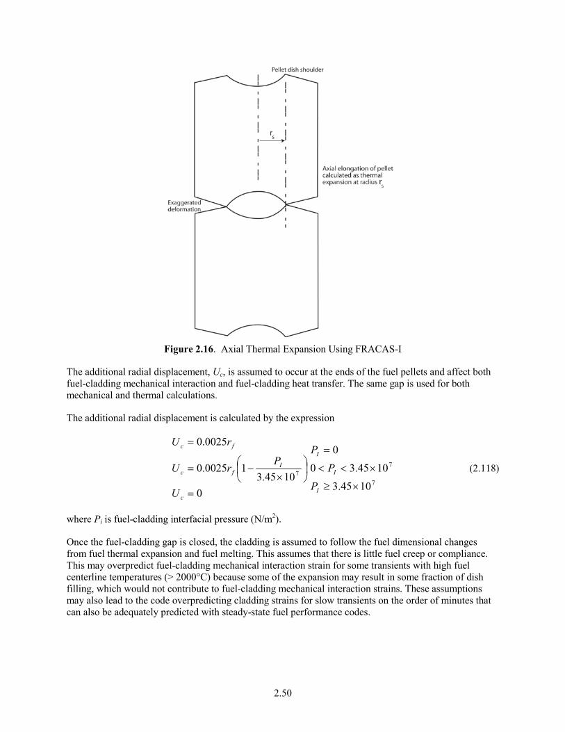
2.50

Figure 2.16. Axial Thermal Expansion Using FRACAS-I

The additional radial displacement, Uc, is assumed to occur at the ends of the fuel pellets and affect both fuel-cladding mechanical interaction and fuel-cladding heat transfer. The same gap is used for both mechanical and thermal calculations.

The additional radial displacement is calculated by the expression

01045.3

10025.0

0025.0

7

=

×−=

=

c

Ifc

fc

U

PrU

rU

7

7

1045.3

1045.30

0

×≥

×<<

=

I

I

I

PP

P (2.118)

where Pi is fuel-cladding interfacial pressure (N/m2).

Once the fuel-cladding gap is closed, the cladding is assumed to follow the fuel dimensional changes from fuel thermal expansion and fuel melting. This assumes that there is little fuel creep or compliance. This may overpredict fuel-cladding mechanical interaction strain for some transients with high fuel centerline temperatures (> 2000°C) because some of the expansion may result in some fraction of dish filling, which would not contribute to fuel-cladding mechanical interaction strains. These assumptions may also lead to the code overpredicting cladding strains for slow transients on the order of minutes that can also be adequately predicted with steady-state fuel performance codes.

2.51

Fuel pellet cracking, beginning with the initial ascension to power, promotes an outward radial relocation (movement) of the pellet fragments that causes additional gap closure. A simplified relocation model is provided in FRAPTRAN that is based on the model used in FRAPCON (Lanning et al. 1997). The model used in FRAPTRAN is as follows: if burnup = 0, relocation = 0.3* gap if burnup > 0, relocation = 0.45* gap

where gap is the as-fabricated radial fuel-cladding gap. Because of the rapid nature of transients, no recovery of the relocation is allowed by FRAPTRAN, whereas FRAPCON does allow some recovery under some conditions. The application of this model to fuel rods with diametral cold gaps of 0.005 inch or less may result in premature gap closure, fuel-cladding mechanical interaction, and underpredicted fuel temperatures.

If FRAPTRAN is initialized using a FRAPCON file, then relocation is included in the burnup-dependent radial dimensions and the above model is bypassed.

The fuel crack volume is the sum of the volume of the fuel radial cracks. The cracks create space which is occupied by the fuel rod internal gas. Axial cracks are not considered. Closed radial cracks are assumed to exist in the fuel even in the cold state. As the fuel temperature rises, the cracks open, with the crack widths increasing with radius. The width of the radial cracks is the difference between the circumferential change caused by radial displacement and circumferential thermal expansion. The total width is independent of the number of cracks and is calculated by

−=∆ ∫ )]([)]([2)(

0

rTrdrrTrc T

r

T εεπ (2.119)

where Δc(r) is the sum of widths of all radial cracks at radius r.

The first term in the parentheses in Equation (2.119) is the circumference change at cold state radius r due to the radial displacement. The second term is the circumferential change due to circumferential thermal expansion.

The volume of the radial cracks is

∫ ∆=fr

oCR drrcV )( (2.120)

The open porosity of the fuel is empirically correlated with fuel density. The open porosity is multiplied by the fuel volume to determine the volume of gas in the fuel pores that is connected to the fuel-cladding gap. This quantity is used in the calculation of fuel rod internal gas pressure.

Depending on fuel density, one of the following correlations is used to calculate fuel open porosity:

2.52

0)25.95(1020196.1

)25.1(1052442.1)25.1(1071836.8)25.1(232855.09297.16

3

3524

=−×=

−×+−×−

−−=

−

−−

PDP

DDDP

25.9525.955.92

5.92

>≤≤

<

DD

D (2.121)

where P = open porosity of fuel (fraction of theoretical volume) D = fuel density (percentage of theoretical maximum density)

2.4.4 Cladding Ballooning Model

After the cladding deformation has been calculated by FRACAS-I, a check is made to determine whether or not the cladding ballooning model should be used. The check consists of comparing the cladding effective plastic strain, which is part of the calculated deformation, with the cladding instability strain given by MATPRO (Hagrman et al. 1981). If the cladding effective plastic strain is greater than the cladding instability strain, the ballooning model, BALON2, is used to calculate the localized, nonuniform straining of the cladding. Refer to Hagrman (1981) for the details of the BALON2 model. Once the instability strain is reached in one node, no further strain is calculated by FRACAS-I for any nodes. The BALON2 model divides the ballooning node into 12 radial and 12 axial subnodes as seen in Figure 2.17. For the node that has reached the instability strain, the radial average hoop, axial, and radial strains at the axial subnode with the maximum hoop strain calculated by BALON2 is used as the hoop, axial, and radial strains for the ballooning node.

BALON2 calculates the extent and shape of the localized large cladding deformation that occurs between the time that the cladding effective strain exceeds the instability strain and the time of cladding rupture. The cladding is assumed to consist of a network of membrane elements subjected to a pressure difference between the inside surface and the outside surface, as shown in Figure 2.17. The equations for the model are derived from the thin shell membrane equilibrium equation and geometric constraints. In addition, the model calculates the temperature rise of the cladding due to heat transfer across the fuel-cladding gap. The fuel surface is assumed to have a nonuniform temperature. The model accounts for the extra cooling the cladding receives as it bulges outwardly.

2.53

Figure 2.17. Description of the BALON2 Model

The BALON2 model predicts failure in the ballooning node when the cladding true hoop stress exceeds an empirical limit that is a function of temperature. This correlation is shown in Figure 2.18. Although the data shown in Figure 2.18 are all from Zircaloy, this model is used in FRAPTRAN-2.0 for Zircaloy-2, Zircaloy-4, ZIRLO™, Optimized ZIRLO™ and M5™. Using this limit, FRAPTRAN predicts failure well when compared to measured engineering burst stress at various temperature levels. However, in some cases the calculated failure strain is very large. To avoid this, a second empirical strain limit was added such that FRAPTRAN will predict failure in the ballooning node when the true hoop stress exceeds the stress limit in BALON2, or when the predicted cladding permanent hoop strain exceeds the FRAPTRAN strain limit. The FRAPTRAN strain limit is provided in Equation (2.122).

22.1906331051.710053049.110692798.610587979.1 223649 +−×+×−×= −−− TTTTfailε

940K<T<1200K

1199.2810360497.71023050.61067939.1 22538 +×−×+×−= −−− TTTfailε (2.122)

1200K < T <1700K

544589.0=failε T > 1700K

where εfail = plastic strain at failure (m/m) T = cladding temperature (K)

2.54

0

50

100

150

200

250

300

350

800 900 1000 1100 1200 1300 1400 1500 1600

Temperature, K

True

Hoo

p St

ress

at B

urst

, MPa

BALON2 Model Data

Figure 2.18. True Hoop Stress at Burst that is Used in BALON2 and FRAPTRAN

With these two limits in place, FRAPTRAN predictions agree with both cladding failure stress and strain data. The predictions also agree with or bound the previously published curves from NUREG-0630 (Powers and Meyer 1980). These comparisons are shown in Figures 2.19 through 2.22 for different temperature ramp rates.

2.55

0

20

40

60

80

100

120

140

160

180

200

800 900 1000 1100 1200 1300 1400 1500 1600 1700

Burst Temperature, K

Engi

neer

ing

Bur

st S

tres

s, M

Pa

0-5°C/s5-10°C/s10-15°C/s15-20°C/sFRAPTRAN 5°/s

Figure 2.19. Engineering Burst Stress Data and FRAPTRAN Predictions for Low Heating Rates

0

20

40

60

80

100

120

140

160

180

200

800 900 1000 1100 1200 1300 1400 1500 1600 1700


Engi

neer

ing

Bur

st S

tres

s, M

Pa

20-25°C/s25-30°C/s30+°C/sFRAPTRAN 28 °C/s

Figure 2.20. Engineering Burst Stress Data and FRAPTRAN Predictions for High Heating Rates

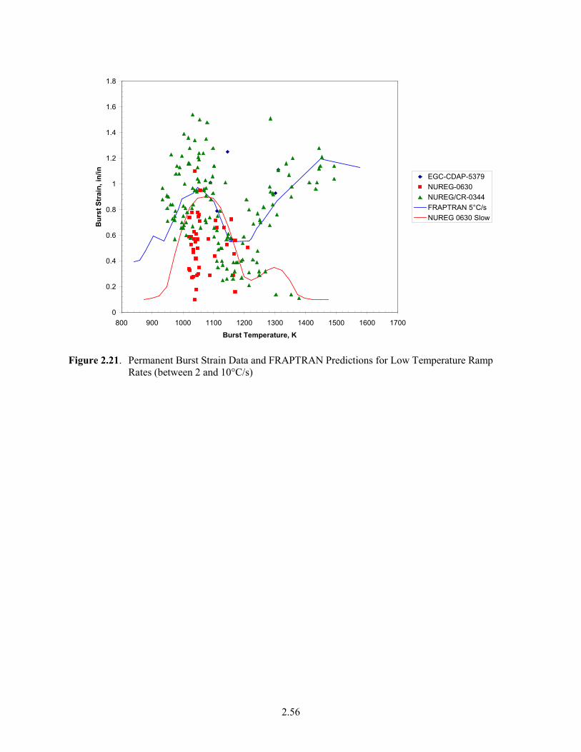
2.56

0

0.2

0.4

0.6

0.8

1

1.2

1.4

1.6

1.8

800 900 1000 1100 1200 1300 1400 1500 1600 1700


Bur

st S

trai

n, in

/in EGC-CDAP-5379NUREG-0630NUREG/CR-0344FRAPTRAN 5°C/sNUREG 0630 Slow

Figure 2.21. Permanent Burst Strain Data and FRAPTRAN Predictions for Low Temperature Ramp

Rates (between 2 and 10°C/s)

2.57

0

0.2

0.4

0.6

0.8

1

1.2

1.4

1.6

1.8

800 900 1000 1100 1200 1300 1400 1500 1600 1700


Bur

st S

trai

n, in

/in EGC-CDAP-5379NUREG-0630Nureg/CR-0344FRAPTRAN1.4 28°C/sNUREG-0630 Fast

Figure 2.22. Permanent Burst Strain Data and FRAPTRAN Predictions for High Temperature Ramp

Rates (greater than 20°C/s)

2.5 Fuel Rod Internal Gas Pressure Response Model

The pressure of the gas in the fuel rod must be known in order to calculate the deformation of the cladding and the transfer of heat across the fuel-cladding gap. The pressure is a function of the temperature, volume, and quantity of gas. Because the temperature is spatially nonuniform, the fuel rod must be divided into several smaller volumes so that the temperature in each small volume can be assumed to be uniform. In particular, the fuel rod is divided into a plenum volume and several fuel-cladding gap and fuel void volumes. The temperature of each volume is given by the temperature model, the size of the volume by the deformation model, and the quantity of gases by the fission gas release model.

The internal gas pressure can be calculated either by a static pressure model (which assumes that all volumes inside the fuel rod equilibrate in pressure instantaneously) or by a transient pressure model which takes into account the viscous flow of the gas in the fuel rod. The static pressure model is the default model. The transient model is an input option. Unless the fuel-cladding gap is small (< 25 μm) or closed, the static and transient models give identical results.

The static fuel rod gas pressure model is based on the following assumptions:

1. The gas behaves as a perfect gas.

2. The gas pressure is the same throughout the fuel rod.

3. The gas in the fuel cracks is at the average fuel temperature.

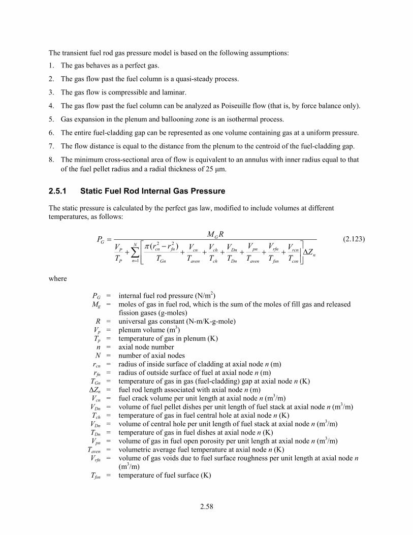
2.58

The transient fuel rod gas pressure model is based on the following assumptions:

1. The gas behaves as a perfect gas.

2. The gas flow past the fuel column is a quasi-steady process.

3. The gas flow is compressible and laminar.

4. The gas flow past the fuel column can be analyzed as Poiseuille flow (that is, by force balance only).

5. Gas expansion in the plenum and ballooning zone is an isothermal process.

6. The entire fuel-cladding gap can be represented as one volume containing gas at a uniform pressure.

7. The flow distance is equal to the distance from the plenum to the centroid of the fuel-cladding gap.

8. The minimum cross-sectional area of flow is equivalent to an annulus with inner radius equal to that of the fuel pellet radius and a radial thickness of 25 μm.

2.5.1 Static Fuel Rod Internal Gas Pressure

The static pressure is calculated by the perfect gas law, modified to include volumes at different temperatures, as follows:

n

N

n csn

rcn

fsn

rfn

aven

pn

Dn

Dn

ch

ch

aven

cn

Gn

fncn

P

P

GG

ZTV

TV

TV

TV

TV

TV

Trr

TV

RMP∆

++++++

−+

=

∑=1

22 )(π (2.123)

where PG = internal fuel rod pressure (N/m2) Mg = moles of gas in fuel rod, which is the sum of the moles of fill gas and released

fission gases (g-moles) R = universal gas constant (N-m/K-g-mole) Vp = plenum volume (m3) Tp = temperature of gas in plenum (K) n = axial node number N = number of axial nodes rcn = radius of inside surface of cladding at axial node n (m) rfn = radius of outside surface of fuel at axial node n (m) TGn = temperature of gas in gas (fuel-cladding) gap at axial node n (K) ΔZn = fuel rod length associated with axial node n (m) Vcn = fuel crack volume per unit length at axial node n (m3/m) VDn = volume of fuel pellet dishes per unit length of fuel stack at axial node n (m3/m) Tch = temperature of gas in fuel central hole at axial node n (K) VDn = volume of central hole per unit length of fuel stack at axial node n (m3/m) TDn = temperature of gas in fuel dishes at axial node n (K) Vpn = volume of gas in fuel open porosity per unit length at axial node n (m3/m) Taven = volumetric average fuel temperature at axial node n (K) Vrfn = volume of gas voids due to fuel surface roughness per unit length at axial node n

(m3/m) Tfsn = temperature of fuel surface (K)

2.59

Vrcn = volume of gas in voids due to roughness on cladding inside surface per unit length (m3/m)

Tcsn = temperature of cladding inside surface (K)

2.5.2 Transient Internal Gas Flow

Transient flow of gas between the plenum and fuel-cladding gap is calculated by the Poiseuille equation for viscous flow along an annulus according to Equation (2.124). Assumptions inherent in Equation (2.127) are ideal gas, laminar flow, and density based on linear average pressure:

∑=

−=

P

s

I

Ii hg

ii

SP

DDHaT

R

PPm

3

22 )(

m

π (2.124)

where m = mass flow rate (g-moles/s) μ = gas viscosity at temperature TA (N-s/m2) Ti = gas temperature at node I (K) TA = volume-averaged temperature of gas in gas (fuel-cladding) gap (K) ℓI = axial length of node I (m) tgi = fuel-cladding radial gap thickness at node I (m) Ip = number of top axial node Is = number of axial node closest to centroid of gas gap (see Figure 2.23) Ha = Hagen number (defined below) Pp = fuel rod plenum gas pressure (N/m2) Ps = fuel-cladding gap gas pressure (N/m2) R = universal gas constant (N-m/K-g-moles) Dg = mean diameter of fuel-cladding gap (m) Dh = hydraulic diameter of fuel-cladding gap = 2tgi for a small gap (m)

The Hagen number is calculated by:

Ha = 22 + 0.24558/(2tgi - 0.0007874) (2.125) where tgi is in inches.

A plot of the relation between Hagen number and gap width given by Equation (2.125) is shown in Figure 2.24. For gaps smaller than 25 μm, the function is cut off at value of 1177. To calculate the fuel-cladding gap pressure, a modified form of Equation (2.123) is used. The plenum term is deleted and the moles of gas in the fuel-cladding gap is substituted in place of the moles of gas in the fuel rod.

2.60

Figure 2.23. Internal Pressure Distribution with the Gas Flow Model

2.61

0

200

400

600

800

1000

1200

0 1 2 3 4 5 6 7 8 9

Gap thickness, mils

Haga

n nu

mbe

r1177

Ha = 22 + 0.24558/(2tg-0.0007874) Where: Ha = Hagan number fg = gap thickness (inches)

Figure 2.24. Hagen Number Versus Width of Fuel-Cladding Gap

2.5.3 Fission Gas Production and Release

The fill gas composition and pressure at the time of a transient, which is dependent on fission gas release prior to the transient, can be either manually entered by the user or read from a FRAPCON burnup initialization file.

FRAPTRAN has a model to calculate the transient release of fission gases as a function of temperature. FRAPTRAN also has a user input option to specify the fission gas release as a function of time.

The transient release of fission gas is highly dependent on the location of the gas in the fuel pellet, both radially, and in each radial node the location (in the grains versus on the grain boundaries) of the gas. Because of this, the transient gas release model in FRAPTRAN may only be used if initialized with a FRAPCON burnup initialization file. In addition, FRAPCON must have been run with the FRAPFGR model (ngasmod=3 in FRAPCON). This model has been developed specifically to predict the location of fission gas within the pellets. This transient release model is described below:

• All grain boundary gas for a given radial node is released when the temperature exceeds 2000°F (1093°C).

• All gas in the restructured grains (matrix) of the high burnup structure for a given radial node is released when the temperature exceeds 3300°F (1816°C).

• Five percent of the gas in the unrestructured grains (matrix) for a given radial node is released when the temperature exceeds 3300°F (1816°C).

This release model was developed to predict the measured release data from RIA experimental tests in CABRI and NSRR. (See data comparisons in Geelhood and Luscher (2014b).

2.62

A user input option is available (MODEL data block) to specify the fission gas release to the fuel-cladding gap and rod plenum during a transient. The user specifies the rod-average fractional fission gas release as a function of time during the transient. Rod-average burnup is used to calculate the rod-average fission gas production which is available to be released. The released fission gas affects the gas pressure and composition, which in turn affects the transient thermal and mechanical calculations.

2.6 High-Temperature Corrosion

In FRAPTRAN, the initial oxide thickness from the steady-state irradiation can be input to the code, or read from the FRAPCON burnup initialization file. No further waterside corrosion is calculated in FRAPTRAN for typical coolant conditions due to the small time periods modeled in FRAPTRAN. However, during a high-temperature transient, such as LOCA, the cladding temperature can become very hot. In this case, a large corrosion layer could form in a matter of seconds to minutes.

FRAPTRAN contains two high-temperature corrosion models that are selected using input variables. In addition, the option exists to not model high-temperature corrosion. The two high-temperature corrosion models are the Cathcart/Pawel (Cathcart et al. 1977) model and the Baker/Just (Baker and Just 1962) model. Guidance on model selection is given in the input instructions shown in Appendix A. The Cathcart/Pawel model is activated in FRAPTRAN-2.0 when the cladding temperature exceeds 1073K (800°C). The Baker/Just model is activated in FRAPTRAN-2.0 when the cladding temperature exceeds 1000K (727°C). A derivation of these models and discussion of extrapolation to lower temperature than the model was originally validated for is provided in Appendix G. These models are described below.

Both the Cathcart-Pawel and Baker Just models are of the following form:

)/exp(1 RTBAKdt

dK−= (2.126)

where K = oxide thickness (m) t = time (s) T = temperature (K) A, B, R = constants

This equation can be integrated and rearranged to the following form:

tRTBAKK ∆−+= )/exp(2212 (2.127)

where K1 = oxide thickness at beginning of time step (m) K2 = oxide thickness at end of time step (m)

Table 2.4 shows the parameters that are used for the Cathcart-Pawel and Baker-Just models.

2.63

Table 2.4. Constants for Cathcart-Pawel and Baker-Just Models

Constant Cathcart-Pawel Baker-Just A 1.126 × 10-6 m2/s 9.415 × 10-5 m2/s B 1.502 × 105 J/mol 4.550 × 104 cal/mol R 8.314 J/mol-K 1.987 cal/mol-K

For the Cathcart-Pawel model, the user can specify that the weight gain be calculated assuming perfect stoichiometry of the oxide, or by assuming a stoichiometric gradient. (See iStoicGrad on page A.23).

It can be seen from Equation (2.126) that the rate of oxidation is inversely proportional to the oxide layer thickness. In FRAPTRAN there are two ways of treating the initial oxide thickness layer that are selected using the input variable, ProtectiveOxide. If ProtectiveOxide = 0, the initial oxide from steady state is included with the high temperature oxidation, so the rate of oxidation for a previously oxidized rod is lower than for a rod with no oxide. If ProtectiveOxide = 1, the initial oxide from steady-state is not included with the high-temperature oxidation, so the rate of oxidation for a previously oxidized rod is the same as the rate for a rod with no oxide.

FRAPTRAN calculates the oxidation of the outer rod surface and, if the inner cladding surface is in contact with steam (i.e., the rod has burst), the oxidation of the inner rod surface. From these inner diameter (ID) and outer diameter (OD) oxide layer thicknesses, FRAPTRAN calculates the oxygen-stabilized alpha layer, the oxygen uptake, the metal water reactor energy, and equivalent cladding reacted (ECR). For the stress calculations, FRAPTRAN reduces the wall thickness based on the thinning from the oxide layer growth. No strength is attributed to the oxide layer. FRAPTRAN-2.0 includes an option to calculate ID oxidation regardless of rupture above a specified burnup. (See nIDoxide and BuOxide on page A.23).

2.7 Fuel Radial Thermal Expansion Routine

There are two options in FRAPTRAN for calculating radial thermal expansion in the pellet. The input variable, nthermex, is used to select between these two options.

In the first option, when nthermex = 0, thermal expansion strain is used to calculate a displacement in the radial direction. The sum of the radial displacements from the pellet center to edge is the change in radius in the pellet. If the pellets have a central hole, a term which calculates the radius change due to thermal expansion in the circumferential direction along the circumference of the central hole is added to the above sum. This formula is provided as Equation (2.131).

∫+⋅=∆ o

i

r

r TiTi drrTrTrR )]([)]([ εε (2.128)

where ∆R = change in radius due to thermal expansion ri = pellet inner radius ro = pellet outer radius εT[T(r)] = thermal expansion strain at a given radius T = temperature

2.64

The first term in this equation accounts for the radius change due to circumferential thermal expansion along the inside of a pellet central hole. The second term adds up the radius changes due to thermal expansion in the radial direction across the remainder of the pellet.

The second option, when nthermex = 1, is to use the thermal expansion strain to calculate a displacement in the circumferential direction and then calculate the change in radius that would result from the change in circumference. The change in radius is calculated at each point along the fuel radius, and the maximum value of change in radius is taken. The sum of the displacements due to radial thermal expansion is then added to this maximum value for the area beyond the radius of maximum radius change. This formula is provided as Equation (2.129).

∫+⋅=∆ 0 )]([)][(r

r TmTmm

drrTrTrR εε (2.129)

where rm is the radius and the quantity r·εT[T(r)] is maximum.

The first term in this equation accounts for the radius change due to circumferential thermal expansion at the radius that gives the maximum change in radius. The second term adds up the radius changes due to thermal expansion in the radial direction for the remainder of the pellet that is past the radius of maximum change in radius.

For most cases (parabolic temperature distributions) Equation (2.128) provides the maximum value for the displacement of the outer edge of the fuel. However, when a temperature profile is edge peaked, as in a reactivity-initiated accident (RIA) shortly after the power pulse, Equation (2.129) gives a larger value for ∆R than Equation (2.128).

Assessment of cladding permanent hoop strain following an RIA suggests that the hoop strain is best predicted when the second option (nthermex = 1) is used. This option is recommended for RIA cases.

2.8 Cladding Failure Models

FRAPTRAN has two principal models that are used to predict when cladding failure happens. The first failure model is applicable mainly to RIA events where deformation is due to pellet cladding mechanical interaction and the temperature of the cladding is relatively low (< 700K). The second failure model is applicable mainly to LOCA events where deformation is due to gas overpressure and the temperature of the cladding is relatively high (> 700K). In either case, when the code predicts cladding failure, the internal gas is assumed to be steam and the cladding inner surface is allowed to oxidize for axial nodes 6 inches above and below the failed node.

2.8.1 Low-Temperature PCMI Cladding Failure Model

At low temperature, where PCMI is the driving force for cladding deformation, a model based on uniform plastic elongation from irradiated cladding (Geelhood et al. 2008) is used as the failure criteria. This model is a function of temperature and hydrogen concentration and is described below.

),min( 0 HexUEUEUE = Hex < 650 ppm (2.130)

%05.0=UE Hex > 650 ppm

2.65

where UE = uniform plastic elongation (percent) UE0 = 2.2 percent p

exHex HAUE −⋅= Hex > 0

0UEUEHex = Hex = 0 )00927.0exp(1211 TA ⋅−= T < 700K 840803.1=A T > 700K Tp ⋅−= 001783.0355231.1 T < 700K 107131.0=p T > 700K ),0max( SolTotex HHH −=

⋅−

×=T

H Sol 985887.18550exp102.1 5

HTot = total hydrogen in cladding, ppm T = temperature (K)

If the predicted plastic hoop stress for any axial node exceeds the model prediction of uniform elongation based on the hydrogen concentration and average cladding temperature at that axial node, the code assumes the cladding has failed at that node. The cladding average temperature is taken as the average of each of the cladding radial node temperatures. A plot of predicted minus measured uniform plastic elongation data provided in Figure 2.25 versus excess hydrogen (Hex) demonstrates that the uniform elongation model provides a reasonable fit as a function of excess hydrogen level (hydrogen above the solubility limit) in the cladding. Further comparisons to the uniform elongation data are provided in Geelhood et al. (2008). It is noted that this failure model was not adjusted to fit RIA data and does a good job predicting failure and non-failure in RIA tests (Geelhood and Luscher 2014b).

-5-4-3-2-1012345

0 500 1000 1500 2000

Excess Hydrogen, ppm

Pred

icte

d - M

easu

red

UE, %

Axial Tests Burst Tests

Table 2.5. Predicted Minus Measured Uniform Elongation from Irradiated Samples from the PNNL Database as a Function of Excess Hydrogen (293K ≤ T ≤ 755K and 0 ≤ Φ ≤ 14×1025 n/m2)

2.66

2.8.2 High-Temperature Cladding Ballooning Failure Model

In the case of a LOCA, the cladding can fail by ballooning and burst. The BALON2 model is used to model the ballooning in the cladding. FRAPTRAN contains empirical stress and strain limits that it uses to predict when cladding failure will occur. These limits are discussed in detail in Section 2.4.4.

3.1

3.0 User Information

In this section, the code structure and computational scheme of FRAPTRAN are outlined and the input and output information are summarized. The link with the FRAPCON code, which can be used to provide initial fuel rod conditions, is also described. Finally, the user’s means of controlling computation accuracy and computer running time are outlined. This also includes guidance on using the code.

3.1 Code Structure and Solution Routine

FRAPTRAN is a computer code composed of several subcodes that iteratively calculate the interrelated effects of fuel and cladding temperature, fuel rod plenum temperature, fuel and cladding deformation, and rod internal gas pressure. Each subcode comprises the FORTRAN programming of a major FRAPTRAN model. The name and function of principal subcodes are listed in Table 3.1. Some of the subcodes have the same function, and the user can select the subcode to be used. Some of the subcodes are not required, and the user can bypass the use of the subcode, which reduces the computer run time. These options are also noted in Table 3.1. Charts of the overall flow of the computations are shown in Figures 3.1 through 3.3. The input requirements and initialization procedure are shown in Figure 3.1; the temperature, mechanical response, and pressure calculations are shown in Figure 3.2; and the cladding oxidation, local cladding ballooning, and fission gas release calculations are shown in Figure 3.3.

As shown in Figure 3.2, the temperature, mechanical response, and internal gas pressure calculations are performed iteratively so that all significant interactions are taken into account. For example, the deformation of the cladding affects the fuel rod internal gas pressure because the internal volume of the rod is changed. The deformation of the cladding also affects the temperature of the fuel and cladding because the flow of heat from the fuel to the cladding is dependent on the fuel-cladding gap width and interface pressure when the gap is closed.

Table 3.1. Name and Function of Principal FRAPTRAN Subcodes

Subcode Name

Function Select Option

Bypass Option

HEAT Compute temperature of fuel and cladding. no no PLNT Compute temperature of gas in fuel rod plenum. If bypassed, the gas

temperature is set equal to the coolant temperature plus 10K. no yes

DEFORM Compute mechanical response of fuel and cladding using FRACAS-I. Stress-induced deformation of the fuel is not modeled.

no no

GSFLOW Compute the gas pressure in the fuel rod. no no BALON2 Compute localized ballooning of cladding. If bypassed, uniform

cladding straining during ballooning is assumed to occur. yes yes

COBILD Compute oxidation of cladding with best estimate model. If bypassed, no cladding oxidation is assumed to occur.

yes yes

METWRB Same function as COBILD, but modeling conforms to requirement of a licensing audit code.

yes yes

3.2

Figure 3.1. Flowchart of FRAPTRAN (Part 1)


3.3


These and all other interactions are taken into account by repeatedly cycling through two nested loops of calculations until convergence is achieved. In the outside loop, the fuel rod temperature and mechanical response are alternately calculated. On the first cycle through this loop, the gap conductance is calculated using the fuel-cladding gap size from the previous time step.

Then the fuel rod temperature distribution is calculated. This temperature distribution then feeds into the mechanical response calculations and influences such variables as the fuel and cladding thermal expansions and the cladding stress-strain relation. A new fuel-cladding gap is calculated which is used in the gap conductance calculation on the next cycle of calculations. The calculations are cycled until two successive cycles compute the same temperature distribution within the convergence criteria.

The inner loop of calculations, shown in Figure 3.2, is cycled in a manner similar to that used for the outer loop, but with the internal gas pressure being the variable determined by iteration. The fuel rod mechanical response and gas pressure are alternately determined. The temperature distribution remains the same during the inner loop of calculations. On the first cycle through this loop, the mechanical response is calculated using the previous time step gas pressure. Variables that influence the gas pressure solution, such as fuel-cladding gap width and plenum volume, are calculated. Then the gas pressure calculation is made, and an updated cladding internal gas pressure is fed back to the mechanical response calculations. The calculations are cycled until two successive cycles result in the same gas pressure within the convergence criteria.

After the two loops of calculations have converged, cladding oxidation, local cladding ballooning, and fission gas release are calculated. These calculations are performed only once per time step.

3.2 Input Information

The execution of FRAPTRAN must be preceded by the creation of one or more sets of information. The sets of information are listed below:

1. the problem definition data (required)

3.4

2. external coolant condition file (optional)

3. FRAPCON initialization file (optional)

4. FRAPTRAN restart file (optional)

The flowcharts in Figures 3.1 and 3.2 show the positions in the path of calculations at which these sets of information are input to the code. Each set of information is input through a different FORTRAN logical unit. The FORTRAN logical unit for each set of information and the conditions for omitting a data set are provided in Table 3.2.

Table 3.2. Input Information

Data Set Fortran

Logical Unit Conditions for Omitting Problem definition data 5 FRAPTRAN restart file is read. Coolant condition file 4 Cladding surface heat transfer is defined in the problem

definition data or the coolant conditions at the bottom of the fuel rod are defined in the problem definition data.

Initialization file from FRAPCON

22 (a) No previous burnup of fuel rod or, (b) burnup-dependent variables are defined in the problem definition data.

The problem definition data describe the design of the fuel rod, the power of the fuel rod, and, optionally, the values of burnup-dependent variables and the coolant conditions. The design data specify the fuel pellet geometry, fuel density, cladding geometry, and amount and type of fill gas. The power data specify the history and spatial distribution of heat generation in the fuel due to fissioning and the decay of radioactive fission products. In particular, the data specify the time history of the rod-average linear heat generation rate (averaged over rod length), the normalized axial power profile (assumed to be invariant during the time span of a FRAPTRAN calculation), and the axially-dependent normalized radial power profile (assumed to be invariant during the time span of a FRAPTRAN calculation). The burnup-dependent data specify the incurred permanent strain of the cladding (from creep) prior to the transient, the incurred permanent strain of the fuel (from densification and fission-product induced swelling) prior to the transient, and the fill gas pressure and composition. The burnup-dependent data can be omitted and be input instead by reading an initialization file generated by FRAPCON. The coolant condition data specify the pressure, mass flux, and enthalpy of the coolant surrounding the fuel rod. As an alternative, the coolant condition data can specify the cladding surface heat transfer coefficient, coolant temperature, and coolant pressure. The coolant condition data may vary with time and elevation. The coolant condition data can be omitted and be input instead through the reading of a coolant condition file.

The coolant condition file consists of data which describe the conditions of the coolant surrounding the fuel rod. The coolant conditions are normally calculated by a thermal-hydraulic systems analysis code such as RELAP4 (Behling et al. 1981) and the results stored on an output file. The required contents and format of the input file for FRAPTRAN are provided in Appendix B.

Using the initialization file generated by FRAPCON results in overwriting the initial user-input values for burnup dependent variables with values calculated by FRAPCON. A list of the variables written by FRAPCON and read by FRAPTRAN for initializing burnup-dependent variables is provided in Table 3.3. Except for a few variables, the variables are generally a function of axial and radial nodes. This initialization file (FILE22) can be omitted and the burnup-dependent data input instead as part of the problem definition data. This latter option, however, requires a manual processing of the burnup-

3.5

dependent variables from a steady-state fuel performance code or other source. Provided in Table 3.3 is information on how the data provided in the initialization file might be entered manually. Note that some data cannot be readily entered manually (e.g., cladding strains). PNNL recommends using a FRAPCON initialization file to most accurately initialize FRAPTRAN for a case that occurs after some burnup.

Also provided in Table 3.3 is the formatting used by FRAPCON to write the data to the file. This information could be used to generate a routine in a different fuel performance code to generate a file that could be read by FRAPTRAN.

Table 3.3. Variables Written by FRAPCON and Read by FRAPTRAN for Burnup Initialization For each FRAPCON time step, the following information is written to a file. FRAPTRAN then reads the information at the first time step after the time specified in the FRAPTRAN input file (variable trest).

Data Written/Read (unit) Comments Format(a)

Input Variable (Appendix A) if FRAPCON-3 file not used

Time (s) write (22,10) time Number of axial nodes

Number of nodes must be matched by FRAPTRAN (variable naxn)

write (22,20) naxn

Cladding OD oxide layer thickness for each axial node (inch)

write (22,10) (BOSOxideThick(k),k=1,naxn)

odoxid and oxideod

Total hydrogen concentration in cladding for each axial node (ppm)

write (22,10) (CladH2Concen(k-1),k=2,nap1)

cexh2a

Cladding peak temperature, to this point in the history, for each axial node (K)

write (2,10) (CladMaxT(k),k=1,naxn)

No input option

Fuel open porosity for each axial node (fraction)

write (2,10) (OpenPorosity(k),k=1,naxn)

OpenPorosityFraction

Cross-section average fuel burnup for each axial node (MW-s/kg)

write (2,10) (AxBurnup(k),k=1,naxn)

Derived from bup and AxPowProfile

Radial node numbers for fuel surface, cladding ID, and cladding OD

write (2,20) nfofs, ncifs, ncofs

Number of radial nodes defined by nfmesh

3.6



Total quantity of gas in fuel rod, initial plus fission gas release (g-moles)

write (2,10) TotalGasMoles

Defined by gsms or by using gappr0 plus tgas0

Gas composition (fraction): helium, argon, krypton, xenon, hydrogen, air, moisture

write (2,10) (GasFraction(j),j=1,7)

gfrac

Radius to each radial fuel node (ft)

These are subsequently normalized to the FRAPTRAN radial node structure

write (2,10) (radfs(l),l=1,nfofs)

Defined when specify nfmesh and FuelPelDiam

Cladding plastic strain in hoop, axial, and radial directions for each axial node

do ldir=1,3 do k=1,naxn write (2,10) CldPlasStrnFrapcon(k,ldir) end do where: ldir=1=hoop, ldir=2=axial, ldir=3=radial

No input option

Cladding effective plastic strain for each axial node

do k=1,naxn write (2,10) EffStrain(k) end do

No input option

Radial temperature profile for each axial node (°F)

These are subsequently interpolated to match the FRAPTRAN radial node structure

write (22,10) (tempfs(l),l=1,ncofs)

No input option

Net permanent fuel deformation from swelling and densification at each axial node (inch)

write (22,10) (SwellDispl(k),k=1,naxn)

radpel

Net permanent cladding deformation from creep and plastic strain (inch)

write (22,10) (colddec(k),k=1,naxn)

eppinp

Permanent fuel relocation displacement (inch)

write (22,10) (ureloc(k),k=1,naxn)

No input option

Gadolinia content in the fuel (fraction)

write (22,10) gadoln gadoln

3.7



radial burnup profile (MWd/MTU)

Interpolated to define burnup profile at FRAPTRAN nodal structure

do k=1,nt do l=1,nr write (22,10) brnup3(k,l) end do

butemp

Relative radial power profile

Interpolated to define relative radial power profile at FRAPTRAN nodal structure

do k=1,nt do l=1,nr write (22,10) formf(k,l) end do

RadPowProfile

Fission gas on grain boundaries and in outer 5% of standard grains if frapfgr model is selected

write(22,*) ngasr write(22,241) (ansr(k),k=1,ngasr) do j=1,nt write(22,241) (gasavail1(k,j), k=1,ngasr) write(22,241) (gasavail2(k,j), k=1,ngasr) write(22,242) fmgp(j,2) enddo

relfraca

Format statements: 10 format (2x, 30 (e10.4,2x) ); for real variables 20 format (2x, 30 (i5,2x) ); for integer variables (a) Variable names used are those in FRAPTRAN.

3.3 Output Information

The FRAPTRAN output provides a complete description of the fuel rod response to the user-specified transient. This output includes, for example, the fuel and cladding temperature, internal gas pressure, and cladding deformation histories, all of which may be printed. Quantities such as peak cladding temperature and time and location of cladding failure are readily determined from the code output.

A list of the FRAPTRAN output information written to Unit 6 (see Appendix A) is provided in Table 3.4. An example of the code output is provided in Appendix B. Another output option is the generation of a file to be used for graphics plotting. This is discussed further in Section 3.5 and Appendix A.

3.8

Table 3.4. FRAPTRAN Output Information

1. Fuel rod radial and axial temperature distribution 10. Fuel elastic and permanent strains 2. Fuel diameter, fuel-cladding gap thickness, and cladding outer diameter

11. Amount of produced and released fission gases

3. Length change of fuel stack and cladding 12. Fuel rod void volume 4. Pressure of internal fuel rod gas 13. Cladding oxide thickness 5. Cladding surface heat transfer coefficient 14. Energy generated by cladding oxidation 6. Critical heat flux at fuel rod surface 15. Stored energy in fuel 7. Fuel-cladding gap heat transfer coefficient 16. Amount of melted fuel 8. Cladding plastic strain 17. Plenum gas temperature 9. Radial stress at fuel-cladding interface 18. Coolant conditions

3.4 Nodalization, Accuracy, and Computation Time Considerations

The code user has four means of controlling accuracy and computer running time. These are through input specifications of 1) nodalization, 2) temperature convergence criteria, 3) pressure convergence criteria, and 4) time step size.

The nodalization input data specify the locations at which variables such as temperature, stress, and strain are to be calculated. Increasing the number of locations provides greater spatial detail at the expense of longer computer run time and larger storage requirements. The nodalization data consist of axial nodalization and radial nodalization.

The axial nodalization data specify the elevations at which the radial distribution of the fuel rod variables are to be calculated. Each of these elevations is defined as an axial node. The axial nodes are considered to be points on the longitudinal axis of the fuel rod. Unequal spacing of the axial nodes is permitted.

The radial nodes lie in planes that pass through the axial nodes and are perpendicular to the fuel rod axis; that is, the centerline of the fuel rod. The first radial node is at the center of the fuel rod. Other radial nodes are placed at the fuel pellet surface and at the cladding inside and outside surfaces. In addition, an arbitrary number of radial nodes can be placed within the fuel and cladding. Unequal spacing of the radial nodes in the fuel is permitted, and the default situation is a spacing that results in equal-area rings of fuel.

An example of the fuel rod nodalization is shown in Figure 3.4. The axial nodes are numbered from bottom to top. The radial nodes are numbered from the fuel rod centerline to the cladding outside surface.

The computer running time is directly proportional to the number of axial nodes but is not as sensitive to the number of radial nodes. If the number of axial nodes is doubled, the computer running time is doubled. If the number of radial nodes is doubled, the running time is increased approximately 15 percent. In general, about 10 axial nodes and 15 radial nodes in the fuel are recommended for a full-length fuel rod.

If cladding ballooning can occur, and an accurate calculation of the ballooning length is desired, a closely spaced axial nodalization is required in the region of anticipated cladding ballooning. In this region, the axial nodes should not be spaced farther apart than a distance equal to 10 cladding diameters.

3.9

Figure 3.4. Example of Fuel Rod Nodalization

The accuracy of the temperature solution is controlled by the input convergence criterion for the maximum permissible fractional difference1 in temperature calculated by two successive cycles through the temperature-deformation loop, as shown in Figure 3.2. If the temperature difference between the two successive cycles at any point in the fuel rod is greater than the convergence criteria, another cycle of calculations occurs. The temperature calculations, however, are not repeated at the axial nodes for which the temperature differences at all radial nodes were less than the convergence criterion.

The accuracy of the solution for internal gas pressure is controlled by the input convergence criterion for the maximum permissible fractional difference in the internal fuel rod gas pressure calculated by two successive cycles through the deformation-pressure loop of calculations. If the pressure difference between successive cycles is greater than the convergence criterion, another cycle of calculation occurs.

In general, the temperature and pressure convergence criteria should each be set equal to 0.001, which results in an implicit solution of the transient. By making the temperature and pressure accuracies large (> 1), each loop is cycled through only once, which results in an explicit solution of the transient. This approach may reduce computer running time and precludes convergence problems. If sufficiently small time steps are specified, adequate calculational accuracies can be ensured.

The accuracy of the solution for mechanical response is internally fixed and cannot be controlled by the code user. With the FRACAS-I model, if the fuel and cladding are not in contact, a noniterative solution is made and no check for convergence needs to be made. If the fuel and cladding are in contact, the

1Fractional difference is defined as (Tn - Tn-1)/Tn-1, where Tn is the temperature calculated by the n-th cycle through the temperature-deformation loop, and Tn-1 is the temperature calculated by the previous cycle.

3.10

solution for the cladding permanent strains is iterative, with convergence declared after less than a 0.001 fractional difference in permanent strains between two successive iterations.

Both the accuracy and run time of the overall solution are controlled by the time step sizes. The time steps must be small enough so that detail in the power and coolant condition histories is not truncated. If a jump in the state of the fuel rod is occurring, such as a transition from nucleate boiling to film boiling, a small time step is required to accurately model the transition process. On the other hand, because the run time is roughly proportional to the number of time steps required to perform the analysis, the time step should be made as large as possible. Therefore, the minimal run time solution usually requires different time step sizes for different parts of the problem time span.

3.5 Comments and Guidance on Operating FRAPTRAN

Provided in this section is some guidance on operating FRAPTRAN (i.e., time step sizes for particular transients, limits to operation, etc). Additional information may be found in the integral assessment report (Geelhood and Luscher 2014b). The input files for the assessment cases are provided in Appendix B of the integral assessment report, and provide examples of preparing input files.

The mechanical solution scheme in FRAPTRAN is sensitive to rapid strain rates and may not iteratively converge if the time step size is too large during periods of high strain rate. RIA calculations are an example of when this problem might be encountered. If the strain rate is too high, the code will stop and print the following messages:

in the prompt window: “COUPLE: cladding plastic strain increment between time steps is too great for iteration procedure, reduce time step by a factor of 5” in the output file: “COUPLE: cladding plastic strain increment between time steps is too great for iteration procedure, reduce time step by a factor of 5. Execution stopped at time = xxxx”

Experience in running the RIA assessment cases indicates that time steps ≤ 1×10–5 seconds are needed.

Some general guidelines for selecting time step size are as follows:

• For RIAs, time step should be ≤ 1×10–5 seconds beginning with the power increase and continued through at least 1 second.

• For a large-break LOCA, a time step size of about 0.1 is recommended during the first few seconds of the transient when the coolant flow changes rapidly with time.

• For a small-break LOCA, both the power and coolant conditions change slowly with time, so a time step size ≥ 1 second may be used.

• During a period of possible film boiling at any location along the rod, the time step size should be ≤ 0.2 seconds.

• During a period of possible cladding ballooning, the time step size should be ≤ 0.5 seconds.

In general, if difficulties are encountered in having a specific problem converge, the time step size should generally be decreased.

3.11

The input power history and time step size arrays are interpreted differently by the code. The power history array is interpolated along the time history while the time step size is constant until changed. The interpretations are visually presented in Figure A.2.

In the “model” input block (Table A.6), the user can specify time-dependent, rod-average fission gas release (presfgr and relfrac variables) and fuel swelling (TranSwell and FuelGasSwell variables). These are options provided primarily to allow the user to simulate the postulated rapid changes in fission gas release and fuel swelling that might occur during a RIA. The rod-average fission gas release (fractional release with the inventory based on the rod-average burnup) affects both the gas composition and rod gas pressure during the calculation. The fuel swelling input is an adder to the fuel radial thermal expansion. Both sets of array input are interpolated between data points.

The input instructions, Appendix A, identify the option to specify a file (FILE66) for graphics data output. This file is designed to be read by a PNNL-developed routine that works with Excel software. The file name needs to be of the format “stripf.i” where “i” is an alpha-numeric name selected by the user. The Excel routine and user instructions will be provided along with the FRAPTRAN code to users.

Thermal hydraulic boundary condition recommendations are provided as an attachment to the input instructions shown in Appendix A.

4.1

4.0 References

Baker L and LC Just. 1962. Studies of Metal Water Reactions at High Temperatures, III. Experimental and Theoretical Studies of the Zirconium-Water Reaction, ANL-6548, p. 7, Argonne National Laboratory, Argonne, IL.

Basile D, M Beghi, R Chierici, E Salina, and E Brega. 1999. COBRA-EN, An Upgraded Version of the COBRA-3C/MIT Code for Thermal-Hydraulic Transient Analysis of Light Water Reactor Fuel Assemblies and Cores, Report no. 1010/1, Enel SpA, Milano, Italy.

Behling SR, et al. 1981. RELAP4/MOD7: A Computer Program to Calculate Thermal and Hydraulic Phenomena in a Nuclear Reactor or Related Systems, NUREG/CR-1998 (EGG-2089), Idaho National Engineering Laboratory, Idaho Falls, ID.

Bishop AA, RO Sandberg, and LS Tong. 1965. “Forced Convection Heat Transfer at High Pressure after the Critical Heat Flux.” ASME paper 65-HT-31, American Society of Mechanical Engineers, New York.

Bjornard TA and P Griffith. 1977. “PWR Blowdown Heat Transfer,” Symposium on the Thermal and Hydraulic Aspects of Nuclear Reactor Safety, Atlanta, Georgia, November 27–December 2, 1977, Vo1. 1, pp. 17−41, American Society of Mechanical Engineers, New York.

Bromley LA. 1950. “Heat Transfer in Stable Film Boiling.” Chemical Engineering Progress, 46(5):221−226.

Cadek FF, DP Dominicis, HC Yeh, and RH Leyse. 1972. PWR FLECHT Final Report Supplement, WCAP-7931, Westinghouse Electric Corporation, Pittsburgh, PA.

Cathcart JV, RE Pawel, RA McKee, RE Druschel, GJ Yurek, JJ Campbell, and SH Jury. 1977. Zirconium metal–water oxidation kinetics, IV: reaction rate studies, ORNL/NUREG-17, Oak Ridge National Laboratory, Oak Ridge, TN.

Chen JC. 1963. “A Correlation for Boiling Heat Transfer to Saturated Fluids in Convective Flow.” ASME paper 63-HT-34, American Society of Mechanical Engineers, New York.

Chung HM and TF Kasser. 1978. Deformation Characteristics of Zircaloy Cladding in Vacuum and Steam under Transient-Heating Conditions: Summary Report. ANL-77-31 and NUREG/CR-0344, Argonne National Laboratory, Argonne, IL.

Crank J and P Nicolson. 1974. “A Practical Method for Numerical Evaluation of Solutions of Partial Differential Equations of the Heat Conduction Type.” In Proceedings, Cambridge Philosophical Society, 43(1974):50-64.

Cunningham ME, CE Beyer, PG Medvedev, and GA Berna. 2001. FRAPTRAN: A Computer Code for the Transient Analysis of Oxide Fuel Rods, NUREG/CR-6739, Vol. 1, PNNL-13576, Vol. 1, Pacific Northwest National Laboratory, Richland, WA.

Dittus FW and LMK Boelter. 1930. “Heat Transfer in Automobile Radiators of the Tubular Type,” University of California Publications in Engineering, 2(13):443−461.

Geelhood KJ, CE Beyer, and WG Luscher. 2008. PNNL Stress/Strain Correlation for Zircaloy. PNNL-17700, Pacific Northwest National Laboratory, Richland, WA.

4.2

Geelhood KJ, WG Luscher, PA Raynaud, IE Porter. 2015. FRAPCON-4.0: A Computer Code for the Calculation of Steady-State, Thermal-Mechanical Behavior of Oxide Fuel Rods for High Burnup. PNNL-19418, Vol. 1 Rev.2, Pacific Northwest National Laboratory, Richland, WA.

Geelhood KJ and WG Luscher. 2016. FRAPTRAN-2.0 Integral Assessment. PNNL-19400, Vol. 2 Rev. 2, Pacific Northwest National Laboratory, Richland, WA.

Groeneveld DC. 1973. Post-Dryout Heat Transfer at Reactor Operating Conditions. AECL-4513, Atomic Energy of Canada, Ltd., Chalk River Project, Chalk River, Ontario.

Groeneveld DC. 1978 (revised August 1979). An Investigation of Heat Transfer in the Liquid Deficient Regime, AECL-3281, Atomic Energy of Canada, Ltd., Chalk River Project, Chalk River, Ontario.

Groeneveld DC and GGJ Delorme. 1976. “Prediction of Thermal Non-equilibrium in the Post-Dryout Regime.” Nuclear Eng. and Des. 36(1):17−26.

Hagrman DL. 1981. Zircaloy Cladding Shape at Failure (BALON2). EGG-CDAP-5379, EG&G Idaho, Inc., Idaho Falls, ID.

Hagrman DL, GA Reymann, and GE Mason. 1981. A Handbook of Materials Properties for Use in the Analysis of Light Water Reactor Fuel Rod Behavior. MATPRO Version 11 (Revision 2). NUREG/CR-0479 (TREE-1280), prepared by EG&G Idaho, Inc., Idaho Falls, Idaho for the U.S. Nuclear Regulatory Commission, Washington, D.C.

Idaho National Engineering Laboratory (INEL). 1978. RELAP5/MOD7 Blowdown Code, Version 2, Code Development and Analysis Program Report. CDAP-TR-78-036, Idaho National Engineering Laboratory, Idaho Falls, ID.

Knuutila A. 2006. Improvements on FRAPCON-3/FRAPTRAN Mechanical Modeling, VTT-R-11337-06. VTT, Finland.

Kreith F. 1964. Principles of Heat Transfer. 8th Edition, Scranton: International Text Book Company.

Lanning DD and CE Beyer. 2002. “Revised UO2 Thermal Conductivity for NRC Fuel Performance Codes.” Transactions of the American Nuclear Society, 2002 Annual Meeting, Vol. 86, pp 285-287. June 9-13, Hollywood, FL.

Lanning DD, CE Beyer, and CL Painter. 1997. FRAPCON-3: Modifications to Fuel Rod Material Properties and Performance Models for High-Burnup Applications. NUREG/CR-6534 Vol. 1, PNNL-11513, Pacific Northwest National Laboratory, Richland, WA.

Lucuta PG, HS Matzke, and IJ Hastings. 1996. “A Pragmatic Approach to Modeling Thermal Conductivity of Irradiated UO2 Fuel: Review and Recommendations.” Journal of Nuclear Materials 232:166-180.

Luscher WG and KJ Geelhood. 2014. Material Property Correlations: Comparisons between FRAPCON-4.0, FRAPTRAN-2.0, and MATPRO. NUREG/CR-7024 Rev. 1, PNNL-19417 Rev. 1, Pacific Northwest National Laboratory, Richland, WA.

McAdams WH. 1954. Heat Transmission. 3rd Edition, New York: McGraw-Hill Book Company, Inc.

Mendelson A. 1968. Plasticity: Theory and Applications. New York: The Macmillan Company.

4.3

Murphy G. 1946. Advanced Mechanics of Materials. New York: McGraw-Hill Book Company, Inc.

Ohira K and N Itagaki. 1997. “Thermal Conductivity Measurements of High Burnup UO2 Pellets and Benchmark Calculation of Fuel Center Temperature.” In Proceedings of the ANS International Topical Meeting on LWR Fuel Performance, pp. 541-549, March 2−6, 1997, Portland, OR.

Powers DA and RO Meyer. 1980. Cladding Swelling and Rupture Models for LOCA Analysis. NUREG-0630, U.S. Nuclear Regulatory Commission, Washington, D.C.

Prandtl L. 1924. “Spannungsverteilung in Plastischen Koerpern.” In Proceedings of the First International Congress on Applied Mechanics.

Sagrado IC, I Vallejo, and LE Herranz. 2013. Analysis of Experimental RIA Scenarios: CIEMAT Contribution to the OECD RIA International Benchmark. DFN/SN-02/OP-13, CIEMAT, Madrid, Spain.

Scatena GJ and GL Upham. 1973. Power Generation in a BWR Following Normal Shutdown on Loss-of-Coolant Accident Conditions. NEDO-10625, General Electric Co., San Jose, CA.

Shestopalov A, K Lioutov, L Yegorova, G Abyshov, and K Mikitiouk. 1999. Modification of USNRC’s FRAP-T6 Fuel Rod Transient Code for High Burnup VVER Fuel. NUREG/IA-0164 U.S. Nuclear Regulatory Commission, Washington, D.C.

Siefken LJ, CM Allison, MP Bohn, and SO Peck. 1981. FRAP-T6: A Computer Code for the Transient Analysis of Oxide Fuel Rods. NUREG/CR-2148 (EGG-2104), EG&G Idaho, Inc., Idaho Falls, ID.

Siefken LJ, VN Shah, GA Berna, and JK Hohorst. 1983. FRAP-T6: A Computer Code for the Transient Analysis of Oxide Fuel Rods. NUREG/CR-2148 Addendum (EGG-2104 Addendum), EG&G Idaho, Inc., Idaho Falls, ID.

Sparrow EM, AL Loeffler, and HA Hubbard. 1961. “Heat Transfer to Longitudinal Laminar Flow between Cylinders.” Journal of Heat Transfer 83:415.

Stewart CW, JM Cuta, JM Kelly, KL Basehore, TL George, SD Montgomery, and DS Rowe. 1998. VIPRE-01: A thermal-Hydraulic Code for Reactor Cores. Vo1. 1-4, Rev. 4, NP-2411-CCM, Electric Power Research Institute, Palo Alto, CA.

Thom JSR, WM Walker, TA Fallon, and GFS Reising. 1965. “Boiling in Subcooled Water During Flow Up Heated Tubes and Annuli.” Paper #7 presented at the Symposium on Boiling Heat Transfer in Steam Generating Units and Heat Exchangers, Manchester, England, September 15-16, 1965, Institute of Mechanical Engineers, London, UK.

Tong LS and JD Young. 1974. “A Phenomenological Transition and Film Boiling Heat Transfer Correlation.” paper #133.9, Heat Transfer 1974, Vol. IV, Fifth International Heat Transfer Conference, Tokyo, Japan.

Wagner RJ. 1963. HEAT-1: A One-Dimensional Time Dependent or Steady-State Heat Conduction Code, IDO-16867, Philips Petroleum Co, Atomic Energy Division, Idaho Falls, ID.

Wang C. 1953. Applied Elasticity. New York: McGraw-Hill Book Company, Inc.

Appendix A –

Input Instructions for FRAPTRAN

A.1

Appendix A: Input Instructions for FRAPTRAN

This appendix provides the input instructions for FRAPTRAN-2.0 as well as guidance on using options and entering data.

An example input file is provided as Figure A.1; please refer to this figure while reading the following instructions. Lines beginning with * in the first column are comment lines only and are not acted on.

An input file for FRAPTRAN provides three basic sets of information. First, the input and output files used by FRAPTRAN are defined. The defined, and needed, files are:

FILE05: principal FRAPTRAN unit for supplying input data. FILE22: unit for supplying FRAPCON-3 initialization input. This is used to initialize burnup

dependent parameters. This unit is used in conjunction with input parameters inp2 and trest (Table A.2).

FILE06: principal FRAPTRAN unit for output. FILE66: unit used to collect data for plotting. This file is designed to be used with a PNNL-

developed Excel™ plotting program.

These files should be defined first in the input. See Figure A.1 for an example of how to define each of these files. The line beginning /* identifies the end of the input and output file definition.

Second, a title card is supplied, as shown in Figure A.1. The line immediately following the line beginning with /* is reserved for the input case title. Text in column 1-80 will be written in the page header in the output before each time step.

Third, using NAMELIST input format, the parameters of the problem are entered. The NAMELIST input is read in by FRAPTRAN and a formatted input is created in a file called formin. FRAPTRAN then reads the formin file to get the input data it needs.

Input parameter data are entered in data blocks using NAMELIST format. The following tables provide the NAMELIST blocks and the input variables in those blocks. To start a NAMELIST block, state the name of the block beginning with a dollar sign in column 2 of the line (e.g., $iodata3). Then, on the following lines in column 2 or greater, type the variable names with their value after that (i.e., temp=1.2.) Alphanumeric variables must be input in quotes. For example, heat=“on” will set the alphanumeric variable heat to on. When a block is finished, type $end beginning in column 2 in the line after the last piece of data.

In some cases, there are certain variables to set certain options or suboptions. The $model and $boundary data blocks let the user specify options and suboptions for modeling and coolant conditions. In the tables defining the data blocks, variables defining options are typically followed by variables defining suboptions, which are in turn followed by the necessary input variables to implement the suboption. To specify a suboption, the option above it must be turned on. To specify an input variable, the suboption above it must be turned on. The data block flow, thus, is generally as follows:

Option 1

2For readability and differentiation from the other text in this appendix, input variables and some files are identified in the text using lower case and italics; note, however, that italics are not used in the actual input file. 3Namelist input is case sensitive.

A.2

suboption 1a variable variable suboption 1b variable variable Option 2 suboption 2a variable etc.

The default condition for options and suboptions is to be turned off, so the user must actively turn on options and suboptions.

All default values are 0.0 (reals) or 0 (integers) unless specified otherwise in the accompanying tables.

A.3

************************************************************************ * FrapTran, transient fuel rod analysis code * *----------------------------------------------------------------------* * * * CASE DESCRIPTION: Standard Problem #1 * * * * UNIT FILE DESCRIPTION * * ---- ------------------------------------------------ * * -- Input: * * * * -- Output: * * 6 STANDARD PRINTER OUTPUT * * 66 STRIPF FILE FOR GRAFITI * * * * -- Scratch: * * 5 SCRATCH INPUT FILE FROM ECHO1 * * * * Input: FrapTran INPUT FILE * * * ************************************************************************ * * GOESINS: FILE05='nullfile', STATUS='scratch', FORM='FORMATTED', CARRIAGE CONTROL='LIST' * * GOESOUTS: FILE06='stdprob1.out', STATUS='UNKNOWN', CARRIAGE CONTROL='LIST' FILE66='stdprob1.plot', STATUS='UNKNOWN', FORM='FORMATTED', CARRIAGE CONTROL='LIST' /*********************************************************************** Standard Problem #1 $begin ProblemStartTime = 0.0, ProblemEndTime = 20.0, $end start $iodata unitout=1, dtpoa(1)=0.5, dtplta=0.25, pow=1, $end $solution dtmaxa(1)=0.001, 0.0, 0.001, 4.9, 0.01, 5.0, 0.01, 20.0, dtss=1.e5 prsacc=0.001, tmpac1=0.001, maxit=100, noiter=100, epsht1=1.0, zelev=0.5,1.5,2.5,3.5,4.25,4.75,5.25,5.75, 6.25,6.75,7.25,7.75,8.5,9.5,10.5,11.5, nfmesh=11, ncmesh=2 $end $design RodLength=12.0, RodDiameter=0.03517, rshd=0.01008, dishd=0.000625, pelh=0.0251, dishv0=0.0000002, FuelPelDiam=0.0305, roughf=1.14, frden=0.932457, fotmtl=2.0, tsntrk=1883.0, gapthk=3.25e-4, coldw=0.1, roughc=2.16, cldwdc=0.04,fgrns=10.0, ncs=22, spl=0.4583, scd=0.0291, swd=0.006333, vplen=0.00038, gfrac(1)=1.0, gappr0=2243.0, gsms=0.03, $end $power RodAvePower=11.08, 0.0, 3.695, 0.6, 2.01, 2.3, 1.413, 8.7, 0.815, 10.0, 1.902, 13.0, 0.543, 16.3, 0.402, 45.0, AxPowProfile=0.56, 0.0, 1.17, 1.6333, 1.46, 2.7, 1.61, 3.8125, 1.58, 4.9, 1.48, 5.99166, 1.34, 7.075, 1.15, 8.15833, 0.94, 9.25, 0.70, 10.3, 0.36, 12.0, RadPowProfile(1)=0.982,0.00, 0.983, 0.00069723, 0.984, 0.00116205, 0.985, 0.00162687, 0.988, 0.00209169, 0.991, 0.00255651, 0.996, 0.00302133, 1.002, 0.00348615, 1.009, 0.00395097,

Figure A.1. Example of Input Data File Illustrating Necessary Data Lines

A.4

1.017, 0.00441579, 1.03, 0.0046482, RadPowProfile(23)=0.982,0.00, 0.983, 0.00069723, 0.984, 0.00116205, 0.985, 0.00162687, 0.988, 0.00209169, 0.991, 0.00255651, 0.996, 0.00302133, 1.002, 0.00348615, 1.009, 0.00395097, 1.017, 0.00441579, 1.03, 0.0046482, RadPowProfile(45)=0.982,0.00, 0.983, 0.00069723, 0.984, 0.00116205, 0.985, 0.00162687, 0.988, 0.00209169, 0.991, 0.00255651, 0.996, 0.00302133, 1.002, 0.00348615, 1.009, 0.00395097, 1.017, 0.00441579, 1.03, 0.0046482, RadPowProfile(67)=0.982,0.00, 0.983, 0.00069723, 0.984, 0.00116205, 0.985, 0.00162687, 0.988, 0.00209169, 0.991, 0.00255651, 0.996, 0.00302133, 1.002, 0.00348615, 1.009, 0.00395097, 1.017, 0.00441579, 1.03, 0.0046482, RadPowProfile(89)=0.982,0.00, 0.983, 0.00069723, 0.984, 0.00116205, 0.985, 0.00162687, 0.988, 0.00209169, 0.991, 0.00255651, 0.996, 0.00302133, 1.002, 0.00348615, 1.009, 0.00395097, 1.017, 0.00441579, 1.03, 0.0046482, RadPowProfile(111)=0.982,0.00, 0.983, 0.00069723, 0.984, 0.00116205, 0.985, 0.00162687, 0.988, 0.00209169, 0.991, 0.00255651, 0.996, 0.00302133, 1.002, 0.00348615, 1.009, 0.00395097, 1.017, 0.00441579, 1.03, 0.0046482, RadPowProfile(133)=0.982,0.00, 0.983, 0.00069723, 0.984, 0.00116205, 0.985, 0.00162687, 0.988, 0.00209169, 0.991, 0.00255651, 0.996, 0.00302133, 1.002, 0.00348615, 1.009, 0.00395097, 1.017, 0.00441579, 1.03, 0.0046482, RadPowProfile(155)=0.982,0.00, 0.983, 0.00069723, 0.984, 0.00116205, 0.985, 0.00162687, 0.988, 0.00209169, 0.991, 0.00255651, 0.996, 0.00302133, 1.002, 0.00348615, 1.009, 0.00395097, 1.017, 0.00441579, 1.03, 0.0046482, RadPowProfile(177)=0.982,0.00, 0.983, 0.00069723, 0.984, 0.00116205, 0.985, 0.00162687, 0.988, 0.00209169, 0.991, 0.00255651, 0.996, 0.00302133, 1.002, 0.00348615, 1.009, 0.00395097, 1.017, 0.00441579, 1.03, 0.0046482, RadPowProfile(199)=0.982,0.00, 0.983, 0.00069723, 0.984, 0.00116205, 0.985, 0.00162687, 0.988, 0.00209169, 0.991, 0.00255651, 0.996, 0.00302133, 1.002, 0.00348615, 1.009, 0.00395097, 1.017, 0.00441579, 1.03, 0.0046482, RadPowProfile(221)=0.982,0.00, 0.983, 0.00069723, 0.984, 0.00116205, 0.985, 0.00162687, 0.988, 0.00209169, 0.991, 0.00255651, 0.996, 0.00302133, 1.002, 0.00348615, 1.009, 0.00395097, 1.017, 0.00441579, 1.03, 0.0046482, RadPowProfile(243)=0.982,0.00, 0.983, 0.00069723, 0.984, 0.00116205, 0.985, 0.00162687, 0.988, 0.00209169, 0.991, 0.00255651, 0.996, 0.00302133, 1.002, 0.00348615, 1.009, 0.00395097, 1.017, 0.00441579, 1.03, 0.0046482, RadPowProfile(265)=0.982,0.00, 0.983, 0.00069723, 0.984, 0.00116205, 0.985, 0.00162687, 0.988, 0.00209169, 0.991, 0.00255651, 0.996, 0.00302133, 1.002, 0.00348615, 1.009, 0.00395097, 1.017, 0.00441579, 1.03, 0.0046482, RadPowProfile(287)=0.982,0.00, 0.983, 0.00069723, 0.984, 0.00116205, 0.985, 0.00162687, 0.988, 0.00209169, 0.991, 0.00255651, 0.996, 0.00302133, 1.002, 0.00348615, 1.009, 0.00395097, 1.017, 0.00441579, 1.03, 0.0046482, RadPowProfile(309)=0.982,0.00, 0.983, 0.00069723, 0.984, 0.00116205, 0.985, 0.00162687, 0.988, 0.00209169, 0.991, 0.00255651, 0.996, 0.00302133, 1.002, 0.00348615, 1.009, 0.00395097, 1.017, 0.00441579, 1.03, 0.0046482, RadPowProfile(331)=0.982,0.00, 0.983, 0.00069723, 0.984, 0.00116205, 0.985, 0.00162687, 0.988, 0.00209169, 0.991, 0.00255651, 0.996, 0.00302133, 1.002, 0.00348615, 1.009, 0.00395097, 1.017, 0.00441579, 1.03, 0.0046482, $end $model internal='on', metal='on', cathca=1, deformation='on', $end $boundary

heat='on'

Figure A.1. (continued)

A.5

press=12, pbh2(1)=2273.0, 0.00, 1561.0, 0.51, 1405.0, 1.01, 1198.0, 2.15, 1166.0, 2.75, 940.0, 6.95, 908.0, 7.55, 856.0, 8.15, 686.0, 9.87, 568.0, 11.07, 206.0, 15.87, 50.0, 20.07, zone=3, htco=12, tem=12, htclev(1)=3.0, 9.0, 12.0, htca(1,1)=51600.0, 0.00, 166.0, 0.51, 36.0, 1.01, 28.1, 2.15, 120.0, 2.75, 100.0, 6.95, 52.0, 7.55, 5.0, 8.15, 5.0, 9.87, 160.0, 11.07, 60.0, 15.87, 50.0, 20.07, tblka(1,1)=638.3, 0.0, 601.5, 0.51, 587.5, 1.01, 743.8, 2.15, 563.5, 2.75, 537.2, 6.95, 533.1, 7.55, 553.2, 8.15, 1333.8, 9.87, 531.0, 11.07, 384.2, 15.87, 893.2, 20.07, htca(1,2)=62300.0, 0.0, 158.0, 0.51, 36.0, 1.01, 281.0, 2.15, 116.0, 2.75, 100.0, 6.95, 52.0, 7.55, 5.0, 8.15, 5.0, 9.87, 160.0, 11.07, 60.0, 15.87, 50.0, 20.07, tblka(1,2)=638.3, 0.00, 601.5, 0.51, 587.5, 1.01, 743.8, 2.15, 563.5, 2.75, 537.2, 6.95, 533.1, 7.55, 553.2, 8.15, 1333.8, 9.87, 531.0, 11.07, 384.2, 15.87, 893.2, 20.07, htca(1,3)=39300.0, 0.0, 250.0, 0.51, 40.0, 1.01, 281.0, 2.15, 128.0, 2.75, 110.0, 6.95, 52.0, 7.55, 5.0, 8.15, 5.0, 9.87, 160.0, 11.07, 60.0, 15.87, 50.0, 20.07, tblka(1,3)=638.3, 0.0, 601.5, 0.51, 587.5, 1.01, 743.8, 2.15, 563.5, 2.75, 537.2, 6.95, 533.1, 7.55, 553.2, 8.15, 1333.8, 9.87, 531.0, 11.07, 384.2, 15.87, 893.2, 20.07, $end $tuning $end

Figure A.1 (continued)

A.6

Table A.1. $begin Data Block Variables to specify start and end time

Variable (type) Description

Units SI; British

Limitation/Default Value

ProblemStartTime (R)

Start time of calculation. If ncards=0, leave this variable blank.

s Required input

ProblemEndTime (R)

End time of calculation. If ncards=0, leave this variable blank.

s Required input

NRestart (I)

Flag to write a FRAPTRAN restart file. Set to 1 to create a FRAPTRAN restart file.

NA Default = 0

ncards (I)

If ncards=1 (default), a new calculation (cold start) is to be performed. This option is required if the run will use burnup initialization data from FRAPCON-3. If ncards=0, a previous calculation is to be continued. This requires a REQUEST card for TAPE1 which gives the restart tape number. This data block is the only data block read in. If ncards=2, a second transient calculation is performed considering the history effects of a previous transient. The time read on the restart tape is back shifted to zero. This permits analysis of a second transient with initiation at time of zero. The input power and coolant condition histories should assume that a time of zero corresponds with time of transient initiation. The steady state condition of the fuel rod is calculated to determine the fuel rod initial conditions. The input variables that are changed from the first to the second transient are the only required input. In general, the data in the power coolant condition blocks will be different and so needs to be input. The data in the tuning, design, and model selection blocks would usually be the same and so these data blocks can be omitted. In the solution control data block, only the time step history would usually be different. So this variable can be input and the other variables in the data block omitted. The radial and axial nodalization can never be changed.

Default = 1

defsize (I)

Default array size for input arrays. To enter more values for any input array, enter a larger value for defsize.

NA Default = 400

(R)=real, (I)=integer, (C)=character

A.7

Table A.2. $iodata Data Block Variables to specify input parameters


Units SI; British


unitin (I)

Option to specify that the input data are in SI units. Enter a value of unitin=1 for SI input units. If this option is omitted, the input is assumed to be in British units.

Default = 0 (British units)

inp (I)

Option to specify the initialization of burnup dependent variables by reading a FRAPCON created file. Enter a value of inp=1 to turn on. The entire problem must be set up in the input file, with the FRAPCON input just re-setting some burnup dependent variables. FRAPCON data are read from unit 22. FRAPCON writes to a file called restart. The user must define unit 22 and file name in the input deck (as is done for the FRAPTRAN output file). The initialization file from FRAPCON is a formatted file. Both inp and trest must be specified to use a FRAPCON data file.

Default = 0 (no FRAPCON initialization)

trest (R)

trest=FRAPCON problem time for initialization. For example, a FRAPCON problem time of zero corresponds to no burnup, while a time of 9.46e7 seconds (3 years) corresponds to high burnup.

s

Default = 0 (no FRAPCON initialization)

(R)=real, (I)=integer, (C)=character Variables to specify output parameters


Units SI; British


unitout (I)

Option to specify that the output is to be in SI units even though the input is in British units. Enter a value of unitout=1 for SI output units. If this suboption is omitted, the output will be in the same units as the input (i.e., will get SI units out if SI units are specified as input). Note: There is no option for SI input with British output.

Default =0 (output same as specified input units)

dtpoa (R)

Specify the interval of problem time between printouts. dtpoa(1)=time interval between printout at problem time of dtpoa(2) until a new time interval is input. Continue entering data pairs as necessary. If the print interval is constant with time for the entire history, dtpoa(1) is the constant print interval and the balance of the dtpoa input is omitted.

s; s

Default = 100s By default, a maximum of 200 time step pairs is allowed.Use defsize to increase this.

dtplta (R)

Specify the output of a plot file. dtplt(1)=time interval between plot output at problem time of dtplt(2) until a new time interval is input. Continue entering data pairs as necessary. If the plot interval is constant with time for the entire history, dtplt(1) is the constant print interval and the balance of the dtplt input is omitted. If dtplt=0, no plot file is created.

s; s

Default = 0 By default, a maximum of 200 time step pairs is allowed.Use defsize to increase this.

res (R)

Option to specify that a restart file is to be created so that the calculations can be continued at some other time. Enter a value of res=1 to turn on. If this suboption is specified, the contents of file TAPE2 (restart file) must be saved.

Default = 0 (no restart file)

A.8


Units SI; British


pow (R)

Option to specify the printout of the fuel rod state at each step of the first power ramp. Enter a value of pow=1 to turn on. At the initial problem time, the power is increased in 0.05 kW/ft steps from zero power to the power at the initial time.

Default = 0


A.9

Table A.3. $solution Data Block Variables to specify time steps


Units SI; British


dtmaxa (R)

Specify the time step history. dtmaxa(1)=time step size at time dtmaxa(2). Continue entering data pairs as necessary. Each time step size is used until a new time step size is input for a later time; this is illustrated in Figure A.2. The recommended time step sizes for various types of problems are given in Table A.10. If the time step size is constant with time for the entire transient history, dtmaxa(1) is the constant time step size and the balance of the dtmaxa input is omitted. If using FRAPCON initialization of burnup dependent variables, the starting time for a FRAPTRAN calculation [dtmaxa(2)] will be still be 0 seconds, even if trest>0, because dtmaxa is relative to the start of the transient calculation, not the start of the irradiation. The information in Table A.10 is modified as follows: For a small break loss-of-coolant accident (LOCA) such as the TMI-2 accident, a time step of 10 s may be used during the adiabatic heatup period. But during the period of rod quenching for any accident, the time step should be reduced to 0.1 to 0.2 s.

s

Required input. By default, a maximum of 200 time step pairs is allowed.Use defsize to increase this.

dtss (R)

Option to specify the solution of the fuel rod temperature by the steady state equation instead of the transient equation. For accident analysis, this suboption is normally omitted. dtss=time step threshold for steady-state solution. If the time step is equal to or greater than dtss, the steady-state equation is used to solve for the fuel rod temperature Otherwise, the transient equation is used.

s

Default = 1×105 s

(R)=real, (I)=integer, (C)=character Variables to specify convergence criteria


Units SI; British


prsacc (R)

Option to specify an implicit solution. prsacc=maximum fractional change in internal fuel rod pressure between two successive iterations for convergence. The test is (p r+1 – p r)/p r ≤ prsacc, where p r is the pressure calculated by the rth iteration. The implicit solution is recommended. If cladding ballooning is possible, specify a value of 0.001 for prsacc. Whenever film boiling occurs at the cladding surface and fuel rod internal pressure is equal to greater than the coolant pressure, ballooning is possible. If no possibility exists for cladding ballooning, a value of 0.01 may be specified for prsacc.

Default = 0.005

A.10


Units SI; British


tmpac1 (R)

For implicit solution, tmpac1 = maximum fractional change in temperature at any radial node between two successive iterations for convergence.

Default = 0.005

soltyp (R)

Option to specify an explicit solution by soltyp=1. One iteration per time step is performed and no check is made of accuracy of solution. If soltyp = 1, do not input values for prsacc or tmpac1.

Default = 0 (implicit solution)

maxit (I)

Maximum number of iterations in the steady state temperature solution.

Default = 200

noiter (I)

Maximum number of iterations in the transient temperature solution.

Default = 200

epsht1 (R)

Maximum temperature change between iterations on thermal properties before convergence declared.

K; °F

Default = 0.001

(R)=real, (I)=integer, (C)=character Variables to specify nodalization


Units SI; British


naxn (I)

Number of evenly spaced axial nodes, with nodes at mid-point of axial regions; see Figure A.3. zelev variable is not used if specify naxn. When specifying axial nodalization, neither naxn nor zelev have to match the input axial power profile. (When using FRAPCON initialization, naxn must match the number of axial nodes used in the FRAPCON case, with a maximum of 22.)

naxn or zelev are required input, no maximum value for naxn. Do not enter a value for naxn if going to specify axial elevations via zelev.

zelev (R)

Option to specify elevation of axial nodes above the bottom of the rod. naxn variable is not used if specify zelev. The input elevations specify the location of the axial nodes as shown in Figure A.4 (i.e., the axial mid-point of each axial node). Continue entry until all positions are specified.

m; ft

naxn or zelev are required input, no maximum number of values for zelev (for more than 400 values enter a larger value for defsize). Do not enter values if using evenly spaced nodalization via naxn.

nfmesh (I)

Number of equal-area radial nodes in the fuel. fmesh variable is not used if specify nfmesh. The first radial node is placed at the fuel center and the last node at the fuel surface.

nfmesh or fmesh are required input. normally nfmesh ~15; no maximum.

fmesh (R)

Option to specify radii of radial nodes in the fuel; always set fmesh(1)=0. Continue until the radius of each radial node has been specified. The last input radius must equal the fuel pellet radius and account for any permanent fuel dimensional changes (i.e., fuel swelling and densification [see gapthk in $design variables]). nfmesh variable is not used if specify fmesh.

m; ft

nfmesh or fmesh are required input. No maximum number of values for fmesh. (for more than 400 values enter a larger value for defsize)

ncmesh (I)

Number of equal-area radial nodes in the cladding.

ncmesh or cmesh are

required input. ncmesh ~ 2 - 5 No maximum.

A.11


Units SI; British


cmesh (R)

Option to specify radii of radial nodes in the cladding; always set cmesh(1)=cladding inner radius. Continue until the radius of each radial node has been specified. The last input radius must equal the cladding outer radius. cfmesh variable is not used if specify ncmesh.

m; ft

ncmesh or cmesh are required input. No maximum number of values for cmesh. (for more than 400 values enter a larger value for defsize)

nce (I)

Number of radial elements in the cladding. Specify this only if MECHAN=1 (Cladding finite element analysis (FEA) model is selected).

Default=5


A.12

Table A.4. $design Data Block Rod Size


Units SI; British


RodLength (R)

Fuel pellet stack length.

m; ft

Default = 0.0 Required input

RodDiameter (R)

Cladding outer diameter. For a zero burnup case, this is the as-fabricated cladding diameter. If a FRAPCON initialization tape is to be read, the as-fabricated cladding diameter is still input, and then RodDiameter is re-initialized with the FRAPCON results. If manually inputting burnup-dependent values for variables, eppinp should be used to specify the axially varying permanent hoop strain for the cladding resulting from the steady-state irradiation with RodDiameter specifying the initial condition. (If no axial variation is assumed, then RodDiameter may be used to specify the burnup condition if it accounts for the burnup-induced cladding permanent diameter change (i.e., creepdown) at 300K.)

m; ft


gapthk (R)

Radial fuel-cladding gap thickness. For a zero burnup case, this is the as-fabricated radial fuel-cladding gap thickness. If a FRAPCON initialization tape is to be read, a value for radial gap thickness is still input, and then gapthk is re-initialized with the FRAPCON results. If manually inputting axially varying burnup-dependent values for cladding and fuel via eppinp and radpel, the gap thickness is automatically corrected. If no axial variation is assumed or input for a burnup case, then gapthk should account for permanent changes in the radial fuel-cladding gap at 300K due to permanent changes in the cladding and fuel dimensions. Values for gapthk should be based on no change in the cladding thickness from the as-fabricated condition.

m; ft


vplen (R)

Volume of upper plenum, including volume of upper plenum spring. Optional input.

m3; ft3

Default = 0.0

volbp (R)

Volume of lower plenum, including volume of lower plenum spring. Optional input.

m3; ft3

Default = 0.0

(R)=real, (I)=integer, (C)=character See heat option in $model input block to model pellets with a central hole.

Spring Dimensions


Units SI; British


ncs (I)

Number of coils in upper plenum spring. Optional input.

Default = 1

spl (R)

Uncompressed height of upper plenum spring. Optional input.

m; ft

Default = 0.0

scd (R)

Uncompressed outer diameter of upper plenum spring coils. Optional input.

m; ft

Default = 0.0

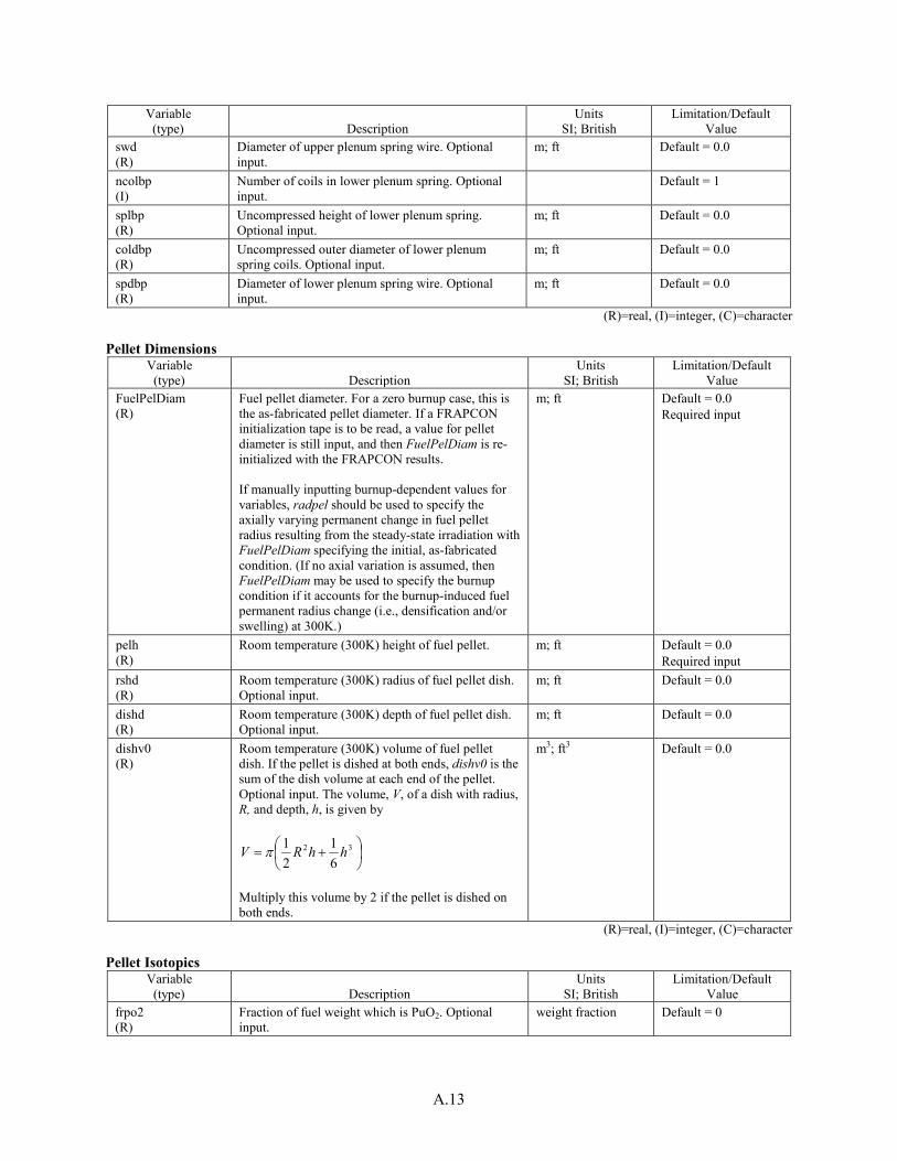
A.13


Units SI; British


swd (R)

Diameter of upper plenum spring wire. Optional input.

m; ft

Default = 0.0

ncolbp (I)

Number of coils in lower plenum spring. Optional input.

Default = 1

splbp (R)

Uncompressed height of lower plenum spring. Optional input.

m; ft

Default = 0.0

coldbp (R)

Uncompressed outer diameter of lower plenum spring coils. Optional input.

m; ft

Default = 0.0

spdbp (R)

Diameter of lower plenum spring wire. Optional input.

m; ft

Default = 0.0

(R)=real, (I)=integer, (C)=character Pellet Dimensions


Units SI; British


FuelPelDiam (R)

Fuel pellet diameter. For a zero burnup case, this is the as-fabricated pellet diameter. If a FRAPCON initialization tape is to be read, a value for pellet diameter is still input, and then FuelPelDiam is re-initialized with the FRAPCON results. If manually inputting burnup-dependent values for variables, radpel should be used to specify the axially varying permanent change in fuel pellet radius resulting from the steady-state irradiation with FuelPelDiam specifying the initial, as-fabricated condition. (If no axial variation is assumed, then FuelPelDiam may be used to specify the burnup condition if it accounts for the burnup-induced fuel permanent radius change (i.e., densification and/or swelling) at 300K.)

m; ft


pelh (R)

Room temperature (300K) height of fuel pellet.

m; ft


rshd (R)

Room temperature (300K) radius of fuel pellet dish. Optional input.

m; ft

Default = 0.0

dishd (R)

Room temperature (300K) depth of fuel pellet dish. Optional input.

m; ft

Default = 0.0

dishv0 (R)

Room temperature (300K) volume of fuel pellet dish. If the pellet is dished at both ends, dishv0 is the sum of the dish volume at each end of the pellet. Optional input. The volume, V, of a dish with radius, R, and depth, h, is given by

+= 32

61

21 hhRV π

Multiply this volume by 2 if the pellet is dished on both ends.

m3; ft3

Default = 0.0

(R)=real, (I)=integer, (C)=character Pellet Isotopics


Units SI; British


frpo2 (R)

Fraction of fuel weight which is PuO2. Optional input.

weight fraction

Default = 0

A.14

fotmtl (R)

Ratio of fuel oxygen atoms to uranium and plutonium atoms. Optional input.

non-dimensional

Default = 2.0

gadoln (R)

Weight fraction of gadolinia (Gd2O3) in fuel pellets. Optional input. May input one value for entire pellet stack or input values as an array for each axial node starting at the bottom.

weight fraction

Default = 0.0

(R)=real, (I)=integer, (C)=character Pellet Fabrication/Conditions


Units SI; British


roughf (R)

Arithmetic mean roughness of fuel pellet surface. Optional input.

μm

Default = 2.0

frden (R)

Fractional theoretical density of fuel pellet.

non-dimensional

Required input Default = 0.0

OpenPorosityFraction (R)

Option to specify the fuel open porosity fraction. If the default value of 0.0 is used, FRAPTRAN will use an internal correlation of open porosity fraction as a function of density (see Section 2.4.3.3). If a positive, non-zero value is entered for OpenPorosityFraction, that value will override the internal calculation of the open porosity fraction.

non-dimensional

Default = 0.0

bup (R)

Rod-average burnup of fuel. Optional input. Needed if user a) wants to use non-zero burnup value of fuel relocation, or b) specifies time-dependent fission gas release history in the model data block. This variable does not need to be entered if using FRAPCON initialization

MWs/kg (GWd/MTU*86400)

Default = 0.0

tsntrk (R)

Fuel sintering temperature. Optional input.

K

Default = 1883.

fgrns (R)

Fuel grain size. Optional input and not used in FRACAS-I.

μm

Default = 10.

radpel (R)

radpel(1) = positive deviation from nominal fuel pellet radius (FuelPelDiam/2) at an elevation of radpel(2). Enter the radius deviation versus elevation pairs until the deviation has been specified along the entire length of the rod. radpel should account for permanent changes in the fuel pellet radius at 300K (i.e., densification and swelling, but not fuel outward relocation). The code checks for negative gap thickness values resulting from the use of radpel and eppinp.

m, m; ft, ft

Default = 0.0 (no deviation)

(R)=real, (I)=integer, (C)=character Cladding Fabrication/Conditions


Units SI; British


A.15


Units SI; British


CladType (I)

Type of cladding used for mechanical and thermal cladding properties. CladType=2 – Zircaloy-2 CladType=3 – Optimized ZIRLO CladType=4 – Zircaloy-4 CladType=5 – ZIRLO CladType=6 – Zr-1%Nb from RRC-KI CladType=7 – M5 CladType=8 – E-110 from RRC-KI

non-dimensional

Default = 4

coldw (R)

Reduction of cross-sectional area of cladding by cold working process (cold work factor for strength). Optional input. Recommended value is 0.5 for cold-worked stress-relieved Zircaloy. coldw=(Ao-A)/Ao where Ao = cross-sectional area prior to cold working, and A =cross-sectional area after cold working.

non-dimensional

Default = 0.0

roughc (R)

Arithmetic mean roughness of cladding inner surface. Optional input.

μm

Default = 0.5

cfluxa (R)

Axially averaged and time averaged fast neutron flux that cladding was exposed to during lifetime. Fast neutrons are defined to have an energy > 1 MeV. The axial profile of the fast flux is assumed to be the same as the axial power profile unless fluxz is input. Optional input. This variable does not need to be entered if using FRAPCON initialization.

n/m2-s

Default = 0.0

tflux (R)

Time span that cladding is exposed to fast neutron flux. cfluxa*tflux must equal axially averaged fast neutron fluence received by the cladding. Optional input. This variable does not need to be entered if using FRAPCON initialization.

s

Default = 0.0

cldwdc (R)

Cold work factor for ductility; recommended value is 0.04. Optional input.

non-dimensional

Default = 0.0

fluxz (R)

Option to specify the axial profile of the cladding fast neutron flux. fluxz(1)=ratio of fast neutron flux to axially-averaged fast neutron flux at elevation fluxz(2). Continue to enter pairs until fully specified. fluxz(1)*cfluxa*tflux = fast neutron fluence at elevation fluxz(2) This variable does not need to be entered if using FRAPCON initialization.

non-dimensional, m; non-dimensional, ft

Default = 0.0 (no axial flux profile)

eppinp (R)

eppinp(1) = initial cladding permanent hoop strain, relative to RodDiameter at an elevation of eppinp(2). Enter the cladding permanent hoop strain versus elevation pairs until the hoop strain has been specified along the entire length of the rod. eppinp should account for permanent changes in the cladding diameter at 300K (i.e., creepdown).


Default = 0.0 (no initial cladding permanent hoop strain)

A.16

(R)=real, (I)=integer, (C)=character Rod Fill Conditions


Units SI; British


gfrac(1) (R)

Fraction of gas that is helium. The mole fractions of gas components gfrac must sum to 1.0.

mole fraction

Default = 1.0

gfrac(2) (R)

Fraction of gas that is argon.

mole fraction

Default = 0.0

gfrac(3) (R)

Fraction of gas that is krypton.

mole fraction

Default = 0.0

gfrac(4) (R)

Fraction of gas that is xenon.

mole fraction

Default = 0.0

gfrac(5) (R)

Fraction of gas that is hydrogen.

mole fraction

Default = 0.0

gfrac(6) (R)

Fraction of gas that is air.

mole fraction

Default = 0.0

gfrac(7) (R)

Fraction of gas that is water vapor.

mole fraction

Default = 0.0

gsms (R)

Quantity of gas in fuel rod; omit if tgas0 is non-zero

g-moles

Default = 0.0 Either gsms or gappr0 and tgas0 are required input.

gappr0 (R)

As-fabricated fill gas pressure. If tgas0=0, the only use of gappr0 is for guessing gas pressure for initialization and an accurate value, therefore, is not required. If tgaso>0, gappr0 is a term in the calculation of moles of gas in the fuel rod and an accurate value, then, is required.

N/m2; psia


tgas0 (R)

As-fabricated fill gas temperature. If gsms is nonzero, omit.

K; °F


(R)=real, (I)=integer, (C)=character Bundle Dimensions


Units SI; British


pitch (R)

Center-to-center spacing of fuel rods. Normally, this option is omitted. Enter a value > 0 to turn on.

m; ft

Default = 0

pdrato (R)

Ratio of rod pitch to rod outer diameter. Omit if a 17x17 pressurized-water reactor (PWR) bundle. Enter a value > 1.0 to change default.

non-dimensional

Default =1.32

rnbnt (R)

Ratio of balloonable rods to total rods in bundle; normally, this ratio is 0.92. Control rods and water rods are examples of rods which cannot balloon. Omit if a 17x17 PWR bundle. Enter a value > 0.01 to change default.

non-dimensional

Default = 1.0

totnb (R)

Total number of rods in fuel bundle. Omit if a 17x17 bundle. Enter a value > 1.0 to change default.

non-dimensional

Default = 289

(R)=real, (I)=integer, (C)=character Variables pitch, pdrato, rnbnt, and totnb define the option to model the restraint to the cladding ballooning given by adjacent fuel rods. The instability strain is set equal to the rupture strain, so that the full range of cladding ballooning is modeled by the FRACAS-I subcode. The BALON subcode is not used. If option not included, no restraint to rod ballooning is to be modeled. Enter a value of pitch > 0. to turn on this option.

A.17

Table A.5. $power Data Block Power History


Units SI; British


RodAvePower (R)

Rod-average linear heat generation rate history. Input pairs of linear heat generation rate and time; continue until power history is fully defined. The coding interpolates between input pairs of data to define the current rod-average linear heat rate; this is illustrated in Figure A.2. If the powop is specified, RodAvePower must not include power due to decay heat. Also exclude gamma energy not deposited in the fuel rod.

kW/m, s; kW/ft, s

By default, a maximum of 200 power/time pairs is allowed.Use defsize to increase this. Required input

powop (R)

Option to calculate the decay heat by the ANS-5.1 formula and add the decay heat to the power specified by the RodAvePower array. powop is the axially-averaged fuel rod power prior to accident initiation.

kW/m; kW/ft

Default = 0.0

timop (R)

Time at which the fuel rod power was equal to powop (Time of shutdown from time of reactor startup).

s

Default = 0.0

fpdcay (R)

Multiplicative factor applied to power given by the ANS formula; normally, fpdcay=1.

non-dimensional

Default = 1.0

tpowf (R)

Time at which fpdcay is fully applied.

s

Default = 0.0

CladPower (R)

Option to specify heating of the cladding by gamma radiation. CladPower is the ratio of heat generation per unit volume in the cladding to the spatially averaged heat generation per unit volume in the fuel; normally, CladPower.0.01.

non-dimensional

Default = 0.0

fpowr (R)

Multiplicative factor for power. Every power value in RodAvePower is multiplied by fpowr.

Default = 1.0

modheat (R)

Direct moderator heating option to add additional power to the coolant. There are two options: (1) The user can supply a value between 0.0 and 1.0; (2) A value of -1.0 will use an empirical correlation to calculate the gamma-heating fraction for each axial node based on the coolant density

NA Default = 0.02

(R)=real, (I)=integer, (C)=character Axial Power Profile


Units SI; British


NumAxProfiles (I)

Number of axial power profiles.

non-dimensional

Default values = 1; By default, a maximum of 400 axial profiles is allowed.Use defsize to increase this.

ProfileStartTime (R)

Time when each successive axial power profile begins. First profile begins at time zero.

s

Default value = 0.0

A.18


Units SI; British


AxPowProfile (R)

Axial power profile. One profile required. For each profile input pairs of axial power factor (normalized to rod-average) and elevation, beginning from the bottom of the rod; continue until axial power profile is fully defined. The first profile begins at AxPowProfile (1, 1), the second profile at AxPowProfile (1, 2), etc. Input should account for any local variations in power due to enrichment variances, central fuel hole, etc., in addition to axial flux profile. First and last values should be at the top and bottom of the fuel column. FRAPTRAN automatically normalizes the axial power profile. It is not necessary to have the same number of pairs to define the axial power profile as the number of axial fuel nodes; however, each axial power profile must have the same number of pairs.


Required input By default, a maximum of 200 time profile/elevation pairs is allowed.Use defsize to increase this.


A.19

Radial Power Profile Variable

(type) Description Units

SI; British Limitation/Default

Value RadPowProfile (R)

Normalized radial power profiles for each axial node. Required input. Input pairs of radial power factor and radius for bottom axial node, from fuel centerline to edge, and then continue for each axial node. Not required to have the same number of pairs to define the radial profile as the number of radial fuel nodes; however, each radial power profile must have the same number of pairs for each axial node. No time dependencies for radial profiles. The first profile begins at RadPowProfile(1), the second at RadPowProfile(2n+1) where n is the number of pairs in the first profile. This variable does not need to be entered if using FRAPCON3 initialization.

non-dimensional, m NOTE: Fuel radii values must be input in units of meters (m), even if other input is in British units.

Required input if not using FRAPCON3 initialization. By default, a maximum of 200 profile/radius pairs is allowed.Use defsize to increase this.

butemp (R)

Radial burnup profiles for each axial node. Optional input. Input pairs of burnup value and radius for bottom axial node, from fuel centerline to edge, and then continue for each axial node. Not required to have the same number of pairs to define the burnup profile as the number of radial fuel nodes; however, each radial burnup profile must have the same number of pairs for each axial node. The first profile begins at butemp(1), the second at butemp(2n+1), where n is the number of pairs in the first profile. This variable does not need to be entered if using FRAPCON initialization.

MWd/MTM, m NOTE: Fuel radii values must be input in units of meters (m), even if other input is in British units.

Default value is 0.00 MWd/MTM. By default, a maximum of 200 burnup/radius pairs is allowed.Use defsize to increase this.


A.20

Table A.6. $model Data Block Input variables specifying model selections Select option to select suboptions below it, include all variables associated with a selected suboption. Include all the variables under each suboption selected.

Option (type)

Suboption (type)


Units SI; British


nthermex (I)

Option to specify fuel thermal expansion model nthermex=0, calculates pellet radius change by adding the radius change in each ring from radial thermal expansion. nthermex=1, calculates pellet radius change by taking the maximum of the sum of the radius changes from each node inside the current ring due to radial thermal expansion or the radius change due to circumferential thermal expansion for the current ring.

Default = 0; free radial thermal expansion model

relocmodel (C)

Fuel relocation model. There are three models to choose from based on the correlations used in different versions of FRAPCON, plus the ability to turn relocation off. Available inputs: “FRAPCON-3.3” “FRAPCON-3.4” “FRAPCON-3.5” (which is the model used in FRAPCON-4.0) “OFF”

NA Default = “FRAPCON-3.3”

tref (R)

Option to specify the reference temperature that will be used in the calculation of fuel and clad enthalpy.

K,°F Default = 298.15K, 77°F

internal (C)

Option to specify one or more of the rod internal gas models set by the suboptions listed below. Enter a value of internal=‘on’ to turn on.

Default = ‘off’

PlenumTemp (I)

Suboption to specify calculation of plenum gas temperature. Default is for plenum gas temperature set equal to local bulk coolant temperature plus 10°F (5.6K). Enter a value of PlenumTemp=1 to turn on the plenum temperature model described in Section 2.3. Both upper and local plenum gas temperatures are calculated using the selected option.

Default = 0; plenum gas temperature set equal to local bulk coolant temperature plus 10°F (5.6K)

A.21

Option (type)

Suboption (type)


Units SI; British


trise (R)

Plenum temperature rise (over coolant) when using the default plenum temperature model (PlenumTemp=0); Temperature rise (over coolant) of insulator pellet when using the detailed plenum temperature model (PlenumTemp =1)

K, °F Default = 10°F

gasflo (I)

Suboption to model transient flow of gas between fuel rod plenum and cladding ballooning region. Enter a value of gasflo=1 to turn on. If the suboption is omitted, the internal gas pressure is assumed to be spatially uniform inside the fuel rod. Normally, this suboption is omitted. For a reactivity initiated accident, the suboption must be omitted.

Default = 0 If this suboption is specified, at least three axial nodes are required.

prescri (I)

Suboption to prescribe the fuel rod internal gas pressure history. Enter a value of prescri=1 to turn on, and then enter values for gasphs.

Default = 0

gasphs (R)

Specified rod internal gas pressure history; enter pairs of pressure and time until history is specified.

N/m2, s; psi, s

By default, a maximum of 200 pressure/time pairs is allowed.Use defsize to increase this.

presfgr (I)

Suboption to specify fission gas release history as a function of time. presfgr=0 no fission gas release. presfgr=1 specify gas release using relfraca. presfgr=2 use transient gas release model initialized with FRAPFGR model in FRAPCON.4.

Default = 0

relfraca (R)

Specified fission gas release history as a function of time during the transient; enter pairs of rod-average fission gas release fraction and time until the desired history is specified.

fraction, s

By default, a maximum of 200 release fraction/time pairs is allowed.Use defsize to increase this. Must also input a value for bup in $design data block.

explenumv (R)

Suboption to specify the volume of some external plenum volume that is attached to the rod, but held at a prescribed temperature.

ft³, m³

Default = 0.0

A.22

Option (type)

Suboption (type)


Units SI; British


explenumt (R)

Specified external plenum temperature history as a function of time during the transient; enter pairs of external plenum temperature and time until the desired history is specified. Enter a single temperature value to use a constant temperature.

°F, s; K, s

By default, a maximum of 200 temperature/time pairs is allowed.Use defsize to increase this.

prestmp (I)

User supplies the plenum temperature vs time Prestmp=0, Code calculates plenum temperature prestmp=1, User supplies the plenum temperature vs time for the upper plenum only prestmp=2, User supplies the plenum temperature vs time for the lower plenum only prestmp=3, User supplies the plenum temperature vs time for the upper and lower plenums

NA Default = 0

gasths (R)

Plenum temperature history. gasths(x,1) is for the upper plenum and gasths(x,2) is for the lower plenum

°F, s; K, s


A.23

Option (type)

Suboption (type)


Units SI; British


metal (C)

Option to specify a model for metal-water reaction (cladding oxidation). Enter a value of metal= ‘on’ to turn on. If this option is omitted, metal-water reaction is not modeled (variable modmw=1). Normally, this option is specified. In order for non-zero hydrogen concentrations to be considered in any calculation, a value of metal=‘on’ must be used and hydrogen concentrations (cexh2a) entered, even if no metal-water reaction is expected. If the maximum cladding temperature is not expected to exceed 1800K, the CATHCART suboption should be specified. If there is a possibility of complete oxidation of the cladding, the BAKER-JUST suboption should be specified. The CATHCART model is more accurate for cladding temperature less than 1800K, but the BAKER-JUST model is more accurate for cladding temperatures greater than 1800K. For temperatures less than 1800K, the BAKER-JUST model overpredicts the amount of oxidation.

Default = ‘off’

idoxid (I)

Suboption to specify the initial oxide thickness on the inner surface of the cladding; default value is 3×10-6 m (3 μm). Enter a value of idoxid>0 to turn on; idoxid= number of axial nodes, (naxn in $solution) and then enter values for oxideid.

Default value = 0

oxideid (R)

Initial oxide thickness on the inner surface of the cladding. Enter values for each axial node specified by naxn in $solution. Continue entry until values are supplied for all axial nodes.

m Enter values in m even if other input is in British units.

Default value is 3×10-6 m (3 μm).

A.24

Option (type)

Suboption (type)


Units SI; British


odoxid (I)

Suboption to specify the initial oxide thickness on the outer surface of the cladding; default value is 3×10-6 m (3 μm). Enter a value of odoxid>0 to turn on; odoxid= number of axial nodes, (naxn in $solution) and then enter values for oxideod.

Default value = 0

oxideod (R)

Initial oxide thickness on the outer surface of the cladding. Enter values for each axial node specified in data block $solution. Continue entry until values are supplied for all axial nodes.

m Enter values in m even if other input is in British units.

Default value is 3×10-6 m (3 μm).

cexh2a (R)

Suboption to specify initial hydrogen concentration (prior to transient) in cladding for use with the FRAPTRAN 1.0 yield stress model (itransient=0). Enter total hydrogen values for each axial node specified in data block $solution. Continue entry until values are supplied for all axial nodes. The excess hydrogen is determined within the code based on the temperature dependent solubility of hydrogen in Zircaloy.

ppm

Default = 0.0

cathca (R)

Suboption to specify the modeling of the metal-water reaction with the COBILD subroutine and the Cathcart correlation of MATPRO. Enter a value of cathca=1 to turn on. Normally, this suboption is specified. (Variable modmw=0) If neither cathca nor baker is specified, there is no timestep printout of oxide thickness, etc., because no oxidation has been calculated.

Default = 0

iStoicGrad

(I)

Suboption to choose between assuming perfectly stochiometric oxide or a stoichiometry gradient in modeling the weight gain calculated by the Cathcart-Pawel model. iStoicGrad=0 – Cathcart-Pawel model assuming perfect stoichiometry iStoicGrad=1- Cathcart-Pawel model assuming stoichiometry gradient

Default = 0

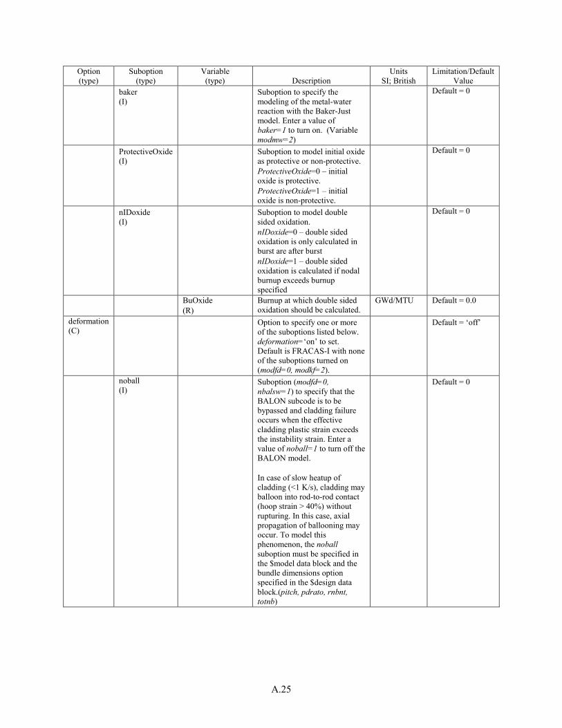
A.25

Option (type)

Suboption (type)


Units SI; British


baker (I)

Suboption to specify the modeling of the metal-water reaction with the Baker-Just model. Enter a value of baker=1 to turn on. (Variable modmw=2)

Default = 0

ProtectiveOxide (I)

Suboption to model initial oxide as protective or non-protective. ProtectiveOxide=0 – initial oxide is protective. ProtectiveOxide=1 – initial oxide is non-protective.

Default = 0

nIDoxide (I)

Suboption to model double sided oxidation. nIDoxide=0 – double sided oxidation is only calculated in burst are after burst nIDoxide=1 – double sided oxidation is calculated if nodal burnup exceeds burnup specified

Default = 0

BuOxide

(R) Burnup at which double sided oxidation should be calculated.

GWd/MTU Default = 0.0

deformation (C)

Option to specify one or more of the suboptions listed below. deformation=‘on’ to set. Default is FRACAS-I with none of the suboptions turned on (modfd=0, modkf=2).

Default = ‘off’

noball (I)

Suboption (modfd=0, nbalsw=1) to specify that the BALON subcode is to be bypassed and cladding failure occurs when the effective cladding plastic strain exceeds the instability strain. Enter a value of noball=1 to turn off the BALON model. In case of slow heatup of cladding (<1 K/s), cladding may balloon into rod-to-rod contact (hoop strain > 40%) without rupturing. In this case, axial propagation of ballooning may occur. To model this phenomenon, the noball suboption must be specified in the $model data block and the bundle dimensions option specified in the $design data block.(pitch, pdrato, rnbnt, totnb)

Default = 0

A.26

Option (type)

Suboption (type)


Units SI; British


TranSwell (I)

Suboption to specify transient fuel swelling history as a function of time during the transient. Enter a value of TranSwell=1 to turn on, and then enter values for FuelGasSwell

Default = 0

FuelGasSwell (R)

Specified fuel swelling history as a function of time during the transient; enter pairs of relative change in fuel radius (i.e., 1.0 = no change in radius due to transient fuel swelling; 1.01 = 1% increase in radius due to transient fuel swelling) and time until the desired history is specified.

fraction, s

Default = 1.0 Maximum of 1000 fuel radii and time pairs.

mechan (I)

Option to select mechanical model. mechan=1 selects FEA model. mechan=2 selects FRACAS-I model l.

Default = 2

frcoef (R)

Coulomb friction coefficient between the cladding and the fuel pellet.

Default = 0.015

irrupt (I)

Rupture model with FEA model. irrupt=0 no hoop strain criterion. irrupt=1 NUREG-0630 fast ramp. irrupt=2 NUREG-0630 slow ramp .

Default = 1

ruptstrain (R)

Maximum effective plastic strain value with FEA model.

in./in.; m/m

Default = 1.0

irefine (I)

Use mesh refinement in case of ballooning with FEA model. irefine=1 yes. irefine=2 no .

Default = 1

refine (R)

Parameter for mesh refinement in FEA model. 2D element axial length divided by its radial length. Increase this parameters for coarser element mesh in ballooning area.

Default=3.0

heat (C)

Option to specify a central void in the fuel pellets. Enter a value of heat=’on’ to turn on.

Default = ‘off’

cenvoi (I)

Suboption to specify that a portion of the fuel pellets have a central void, such as that required to contain a thermocouple to measure the temperature of the center of the fuel. Enter a value of cenvoi=1 to turn on.

Default = 0

A.27

Option (type)

Suboption (type)


Units SI; British


zvoid1 (R)

Distance from bottom of fuel pellet stack to the bottom of the central void.

m; ft

zvoid2 (R)

Distance from bottom of fuel stack to the top of the central void.

m; ft

rvoid (R)

Radius of central void. The radial nodalization as specified in the $solution data block is automatically adjusted to put the second radial node at the surface of the central void.

m; ft

Default = 0

inst (C)

If inst=‘instrument’, the central void is assumed to contain an instrument instead of the fuel rod gas. If no instrument in the central void, omit this variable.

Default = ‘off’


A.28

FRAPTRAN Thermal Hydraulic Input

In FRAPTRAN, the variables that specify the thermal hydraulic boundary conditions for the fuel rod are considerably more complicated than the input variables used in FRAPCON. In FRAPCON, the coolant conditions are specified by three variables that describe the inlet temperature, pressure, and mass flow rate. However, in FRAPTRAN, there are two general methods and considerably more input variables that should be specified to properly model the thermal hydraulic boundary conditions. This document will describe each general method and provide guidance for which method to use for different cases and how to use each general method.

FRAPTRAN $boundary Data Block

The thermal hydraulic boundary conditions are described in FRAPTRAN in the $boundary data block. This data block consists of four options. These options are ‘coolant,’ ‘heat,’ ‘reflood,’ and ‘radiation.’ The following describes how to use these options and when it is appropriate to use them.

‘coolant’ option

The ‘coolant’ option should be used when the coolant is water and the pressure, temperature, and mass flux are known. If this option is used, the ‘heat’ option should not be used. The correlations for the nucleate boiling heat transfer, critical heat flux (CHF), and post-CHF heat transfer in FRAPTRAN-2.0 are such that the default models are applicable to a wide range of temperatures and pressures that may be encountered during accident conditions in boiling-water reactor (BWR) and PWR coolant. The following describes how to set up the required input when using the ‘coolant’ option

• Use the variables under the suboption ‘geomet’ to specify the geometry of the coolant channel. Table A.8 shows how to calculate these parameters based on pitch and rod diameter.

• Specify the coolant pressure history using the variable under the suboption ‘pressu.’

• Specify the coolant mass flux history using the variable under the suboption ‘massfl.’

• Specify the coolant inlet, outlet, or core average enthalpy using the variables under the suboptions ‘lowpl,’ ‘upppl,’ or ‘coreav,’ respectively. Only specify one of these enthalpies. Enthalpy can be determined by using the coolant temperature and pressure to look up enthalpy in a steam table.

• The suboption ‘nucbo’ can be used to specify the nucleate boiling heat transfer correlation. The default value, ‘nucbo=0,’ uses the Thom plus Dittus-Boelter correlation and is recommended.

• The suboption ‘chf’ can be used to specify a critical heat flux correlation. The default value, ‘chf=0,’ uses the EPRI-1 correlation and is recommended.

• The suboption ‘filmbo’ can be used to specify the post-CHF heat transfer correlations to be used in transition and film boiling. The default value, ‘filmbo=0,’ uses the modified Tong-Young and Groeneveld 5.9 correlations for transition and film boiling, respectively, and is recommended.

The ‘coolant’ option models the coolant in a similar fashion to FRAPCON. The additional input necessary for this option is the geometry of the flow channel that can be calculated based on the pitch and rod outer diameter as outlined in Table A.8, and the model selection variables. Descriptions and ranges of applicability for each of these models can be found in Appendix D. However, as discussed above, unless the user has a good reason, the new default values should be selected for all cases when the ‘coolant’ option is selected. Possible reasons for selecting a different model are given below.

• Evaluating the performance of a particular correlation for conditions of interest.

A.29

• Comparing FRAPTRAN to results from other models that use a particular correlation.

• When a particular correlation is known from experience or experimental evidence to be more suitable than the default selection for a particular application.

‘heat’ option

The ‘heat’ option should be used when the coolant is not water, when only cladding surface temperatures are known, or when cladding surface temperatures are known and the focus of the case is to assess the thermal and mechanical performance of a fuel rod given certain boundary conditions. If this option is used, the ‘coolant’ option should not be used. The following describes how to set up the required input when using the ‘heat’ option

• Specify the coolant pressure history using the variable under the suboptions ‘press.’

• Specify the top of axial zones where coolant temperature and heat transfer coefficients will be entered. Note: These zones do not have to correspond with the axial nodes set up previously. The code will interpolate for each axial node.

• For each axial zone, specify the coolant temperature history (tblka) using the variable under the ‘tem’ suboption.

• For each axial zone, specify the heat transfer coefficient history (htca) using the variable under the ‘htco’ suboption.

• To set cladding temperatures, set the coolant temperature equal to the desired cladding temperature, and enter a very large value for the heat transfer coefficient (htca =2.0×106 W/m2-K or 352,222 Btu/ft2-hr-°F).

‘reflood’ option

The ‘reflood’ option can be used to specify a core reflood after loss of coolant. This option may be used in conjunction with either of the ‘coolant’ option or the ‘heat’ option. However, the parameters from the either the ‘heat’ or ‘coolant’ option will only be used by the code before the time specified in the ‘reflood’ option by the variable ‘time.’ After this time the models in the ‘reflood’ option that model adiabatic heatup and reflooding will be used.

‘radiation’ option

The ‘radiation’ option can be used to model a rod within a flow shroud. This option may be used in conjunction with any of the above options and simply adds another layer of resistance between the fuel rod and the coolant.

Recommendations for $boundary Option Selection

Table A.7 gives a list of possible scenarios that may be modeled in FRAPTRAN. This table shows recommendations for the best way to model the thermal hydraulic boundary conditions for these cases.

A.30

Table A.7. Recommendations for Modeling Thermal Hydraulic Boundary Conditions for Various Cases

Case Recommended Option Comments PWR/BWR reactivity-initiated accident (RIA)

‘coolant’ option with default models The ‘coolant’ option with the default values will be used for the entire period.

PWR/BWR LOCA ‘coolant’ option with default models before LOCA, ‘reflood’ option during and after LOCA

For the period prior to the LOCA, the ‘coolant’ parameters will be used. For the period after the coolant empties from the core, the ‘reflood’ parameters will be used.

Cabri sodium loop RIA test ‘heat’ option with measured cladding temperatures set as coolant temperature and high heat transfer coefficient

Since the coolant is sodium, the ‘heat’ option must be used. Measured cladding temperatures are necessary to model these rods.

NSRR sealed water capsule RIA test

‘heat’ option with measured cladding temperatures set as coolant temperature and high heat transfer coefficient

Because measured cladding temperatures are available, they should be used.

BIGR sealed water capsule RIA test

‘coolant’ option with stagnant room temperature water

Measured cladding temperatures are not available. Note: This option will provide reasonable cladding temperatures during the RIA and immediately thereafter, but for more than ½ second after the pulse the predicted cladding temperatures may not be realistic due to localized effects that cannot be modeled in FRAPTRAN.

Table A.8. $boundary Data Block To specify coolant conditions, choose either the ‘coolant’ option or the ‘heat’ option. To specify reflood conditions, choose the ‘reflood’ option. To specify a flow shroud, choose the ‘radiation’ option. ‘coolant’ option. Input variables specifying coolant condition (option 1). Suboptions labeled as required input are only required if the coolant option is selected. Include all the variables under each suboption selected.

Option (type)

Suboption (type)


Units SI; British


coolant (R)

Option to specify pressure, mass flux, and enthalpy of coolant. Enter a value of coolant=‘on’ to turn on. If this option is specified, the heat option and all of its suboptions are omitted.

Default = ‘off’

geomet (I)

Suboption to specify geometry of coolant channel cooling fuel rod. Enter a value of geomet=1 to turn on, and then enter values for dhe, dhy, and achn.

Default = 0 Required input

A.31

Option (type)

Suboption (type)


Units SI; British


dhe (R)

Heated equivalent diameter of flow channel (4*flow area/heated perimeter). The terms in the calculation of dhe are defined in Table A.11.

m; ft

dhy (R)

Hydraulic diameter of flow channel (4*flow area/wetted perimeter).

m; ft

achn (R)

Flow cross-sectional area.

m2; ft2

tape1 (I)

Suboption to specify that coolant conditions are input on file. Enter a value of tape1=1 to turn on. The lowpl, upppl, pressu, and massfl suboptions are omitted. The file is read by Fortran logical unit 4 and must contain data in the format given in Appendix B. The tape1 suboption (option Number 3 of Table A.12) is recommended. Specification of this suboption requires a calculation of the transient fuel rod coolant conditions by a code such as RELAP5. If these calculations cannot be performed, option Number 1of Table A.12 may be used and the coolant enthalpy calculated by FRAPTRAN. The FRAPTRAN calculation of enthalpy is satisfactory for operational transients. But for large and small break LOCAs and RIAs, difficulties in the numerical solution occur. If option Number 1 is specified, the time step should not exceed 0.05 s.

Default = 0 Required input if lowpl or upppl suboptions are not specified

nvol1 (I)

Number of coolant zones stacked on top of each other and surrounding fuel rod. The coolant conditions are assumed uniform within each zone.

nchn (I)

Number of coolant channels in contact with the fuel rod. If coolant conditions are azimuthally uniform, as is normally the case, only one coolant channel borders the fuel rod and the input for nchn is omitted.

lowpl (I)

Suboption to specify the enthalpy history of coolant at bottom of fuel rod (inlet enthalpy). Enter a value of lowpl>0 to turn on; lowpl= number of enthalpy/time pairs. If this suboption is specified, then suboptions pressu, and massfl must also be input.

Default = 0 Required input if tape1 or upppl suboptions are not specified maximum of 1000 enthalpy-time pairs

hinta (R)

Inlet enthalpy and time data pairs. Continue until the inlet enthalpy history is defined for the time range of the problem. (lowpl data pairs)

J/kg, s; Btu/lbm, s

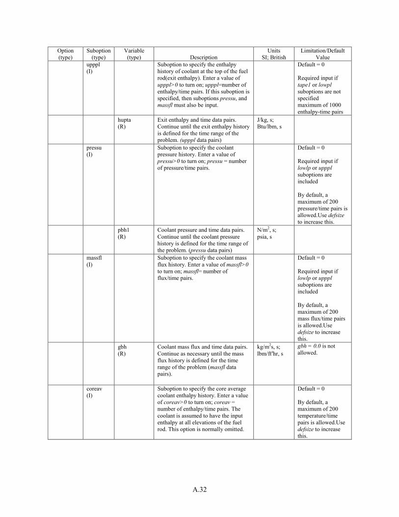
A.32

Option (type)

Suboption (type)


Units SI; British


upppl (I)

Suboption to specify the enthalpy history of coolant at the top of the fuel rod(exit enthalpy). Enter a value of upppl>0 to turn on; upppl=number of enthalpy/time pairs. If this suboption is specified, then suboptions pressu, and massfl must also be input.

Default = 0 Required input if tape1 or lowpl suboptions are not specified maximum of 1000 enthalpy-time pairs

hupta (R)

Exit enthalpy and time data pairs. Continue until the exit enthalpy history is defined for the time range of the problem. (upppl data pairs)

J/kg, s; Btu/lbm, s

pressu (I)

Suboption to specify the coolant pressure history. Enter a value of pressu>0 to turn on; pressu = number of pressure/time pairs.

Default = 0 Required input if lowlp or upppl suboptions are included By default, a maximum of 200 pressure/time pairs is allowed.Use defsize to increase this.

pbh1 (R)

Coolant pressure and time data pairs. Continue until the coolant pressure history is defined for the time range of the problem. (pressu data pairs)

N/m2, s; psia, s

massfl (I)

Suboption to specify the coolant mass flux history. Enter a value of massfl>0 to turn on; massfl= number of flux/time pairs.

Default = 0 Required input if lowlp or upppl suboptions are included By default, a maximum of 200 mass flux/time pairs is allowed.Use defsize to increase this.

gbh (R)

Coolant mass flux and time data pairs. Continue as necessary until the mass flux history is defined for the time range of the problem (massfl data pairs).

kg/m2s, s; lbm/ftshr, s

gbh = 0.0 is not allowed.

coreav (I)

Suboption to specify the core average coolant enthalpy history. Enter a value of coreav>0 to turn on; coreav = number of enthalpy/time pairs. The coolant is assumed to have the input enthalpy at all elevations of the fuel rod. This option is normally omitted.

Default = 0 By default, a maximum of 200 temperature/time pairs is allowed.Use defsize to increase this.

A.33

Option (type)

Suboption (type)


Units SI; British


hbh (R)

Core average coolant enthalpy and time data pairs. Continue as necessary until the core average coolant enthalpy history is defined for the time range of the problem. (coreav data pairs)

J/kg, s; Btu/lbm, s

nucbo (I)

Suboption to select the nucleate boiling heat transfer correlation to be used. Enter a value of nucbo=1 to turn on. The correlations available are described in Appendix D. If this suboption is omitted, the Thom correlation is used.

Default = 0; Thom plus Dittus-Boelter correlation is used.

nbhtc (I)

Indicator for nucleate boiling heat transfer correlation to be used. nbhtc = 0 selects the Thom plus Dittus-Boelter correlation. nbhtc = 1 selects Chen correlation. Both correlations are continuous from subcooled to fully saturated nucleate boiling. No distinction needed between subcooled and saturated nucleate boiling.

Default = 0 (Thom plus Dittus-Boelter correlation)

chf (I)

Suboption to select the CHF correlation to be used. Enter a value of chf=1 to turn on. The correlations are described in Appendix D. If this suboption is omitted, the EPRI-1 correlation is used.

Default = 0 (EPRI-1 correlation)

jchf (I)

Indicator of CHF correlation to be used. For both PWR and BWR, the EPRI-1 correlation is recommended. For flow rate < 0.2 Mlbm/hr-ft2, modified Zuber is used. For high void fraction (>0.8), Biasi is used. jchf= ‘0’ selects the EPRI-1 correlation. jchf=‘1’ selects the Bowring mixed flow cluster correlation. jchf=‘2’ selects the MacBeth correlation. jchf=‘3’ selects the Biasi correlation. jchf=‘4’ selects the modified Zuber correlation.

See Table D.3 in Appendix D of NUREG/CR-6739, Vol.1, FRAPTRAN: A Computer Code for the Transient Analysis of Oxide Fuel Rods, to select a model that is applicable to the coolant conditions and flow channel geometry.

A.34

Option (type)

Suboption (type)


Units SI; British


filmbo (I)

Suboption to select the post-CHF heat transfer correlations to be used in transition and film boiling. Enter a value of filmbo=1 to turn on. The correlations are described in Appendix D. If this suboption is omitted, modified Tong-Young is selected for transition boiling and Groeneveld 5.9 is used for film boiling. If flow rate < 0.2 Mlbm/hr-ft2, modified Bromley is used. If the tape1 suboption is specified, it is recommended that the film boiling correlation be the same as that used in the calculations which produced the coolant condition tape.

Default = 0 (modified Tong-Young and Groeneveld 5.9 correlations, for transition and film boiling, respectively)

jfb (I)

jfb is the indicator of the film boiling correlation to be used. jfb=‘0’ selects the Groeneveld 5.9 correlation (the cluster geometry form of the correlation). jfb=‘1’ selects the Groeneveld 5.7 correlation (the open annulus form of the correlation). jfb=‘2’ selects the Bishop-Sandburg-Tong correlation. jfb=‘3’ selects the Groeneveld-Delorme correlation.

Default = 0 (Groeneveld 5.9 correlation)

jtr (I)

jtr is the indicator of the transition boiling correlation to be used. jtr=0 selects the modified Tong-Young correlation. jtr=1 selects the modified Condie-Bengston correlation. jtr=2 selects the Bjornard-Griffith correlation.

Default = 0 (Tong-Young)

coldwa (I)

Suboption to modify the critical heat flux for cold wall effect. Enter a value of coldwa=1 to turn on. Normally, this suboption is omitted

Default = 0

axpow (I)

Suboption to modify the critical heat flux for effect of axially varying power. Enter a value of axpow=1 to turn on. If flow reverses, suboption is automatically turned off.

Default = 0

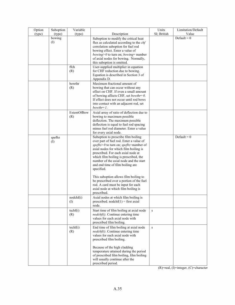
A.35

Option (type)

Suboption (type)


Units SI; British


bowing (I)

Suboption to modify the critical heat flux as calculated according to the chf correlation suboption for fuel rod bowing effect. Enter a value of bowing>0 to turn on; bowing= number of axial nodes for bowing. Normally, this suboption is omitted.

Default = 0

ffch (R)

User-supplied multiplier in equation for CHF reduction due to bowing. Equation is described in Section 3 of Appendix D.

bowthr (R)

Maximum fractional amount of bowing that can occur without any effect on CHF. If even a small amount of bowing affects CHF, set bowthr=0. If effect does not occur until rod bows into contact with an adjacent rod, set bowthr=1.

ExtentOfBow (R)

Axial array of ratio of deflection due to bowing to maximum possible deflection. The maximum possible deflection is equal to fuel rod spacing minus fuel rod diameter. Enter a value for every axial node.

spefbz (I)

Suboption to prescribe film boiling over part of fuel rod. Enter a value of spefbz>0 to turn on; spefbz=number of axial nodes for which film boiling is prescribed. For each axial node at which film boiling is prescribed, the number of the axial node and the start and end time of film boiling are specified. This suboption allows film boiling to be prescribed over a portion of the fuel rod. A card must be input for each axial node at which film boiling is prescribed.

Default = 0

nodchf(i) (I)

Axial nodes at which film boiling is prescribed. nodchf(1) = first axial node.

tschf(i) (R)

Start time of film boiling at axial node nodchf(i). Continue entering time values for each axial node with prescribed film boiling.

s

techf(i) (R)

End time of film boiling at axial node nodchf(i). Continue entering time values for each axial node with prescribed film boiling. Because of the high cladding temperature attained during the period of prescribed film boiling, film boiling will usually continue after the prescribed period.

s


A.36

$boundary data block, ‘heat’ option Input variables specifying coolant condition (option 2) Suboptions labeled as required input are only required if the heat option is selected. Include all the variables under each suboption selected.

Option (type)

Suboption (type)


Units SI; British


heat (C)

Option to specify the heat transfer coefficient at the cladding outer surface. Enter a value of heat=‘on’ to turn on. If this option is specified, the coolant option and all of its suboptions are omitted.

Default = ‘off’

tape2 (I)

Suboption to specify that the heat transfer coefficients, coolant temperature, and pressure are input on tape. Enter a value of tape2=1 to specify. All of the other suboptions are omitted. The tape is read by Fortran logical unit 4 and must contain data in the format given in Appendix B.

Default = 0 Required input if all other suboptions are omitted

nvol2 (I)

Number of heat transfer coefficient zones stacked on top of each other. The heat transfer coefficient, coolant temperature, and pressure are assumed uniform within each zone.

fltgap2 (R)

Gap multiplier.

press (I)

Suboption to specify coolant pressure. Enter a value of press>0 to turn on; press= number of pressure/time pairs.

Default = 0 Required input if tape2 suboption is not specified By default, a maximum of 200 pressure/time pairs is allowed.Use defsize to increase this.

pbh2(i) (R)

Coolant pressure and time data pairs. Continue as necessary to specify coolant pressure history.

N/m2, s; psia, s

zone (I)

Suboption to specify the elevation of heat transfer coefficient zone 1. FRAPTRAN will interpolate to the midpoint of each axial node to determine the heat transfer conditions for each axial node. Enter a value of zone>0 to turn on; zone= number of heat transfer coefficient zones.

Default = 0 Required input if tape2 suboption is not specified By default, a maximum of 400 heat transfer zones is allowed.Use defsize to increase this.

htclev(i) (R)

Array of elevations of each heat transfer coefficient zones specified by zone.

m, ft

A.37

Option (type)

Suboption (type)


Units SI; British


htco (I)

Suboption to specify heat transfer coefficient history for zones. Enter a value of htco>0 to turn on; htco=number of heat transfer coefficient/time pairs. Enter as a single value if the same number of pairs will be entered for each zone. Enter an array if the number of pairs will be different for each zone

Default = 0 Required input if tape2 suboption is not specified By default, a maximum of 200 HTC/time pairs is allowed.Use defsize to increase this.

htca(i,j) (R)

Heat transfer coefficient and time data pairs for zones. Continue as necessary to specify heat transfer coefficient history for zones. htca(1,1) starts input for zone 1 htca(1,2) starts input for zone 2.

W/m2K, s; Btu/ft2hr°F, s

tem (I)

Suboption to specify coolant temperature history for zone 1. Enter a value of tem>0 to turn on; tem=number of temperature/time pairs. Enter as a single value if the same number of pairs will be entered for each zone. Enter an array if the number of pairs will be different for each zone

Default = 0 Required input if tape2 suboption is not specified By default, a maximum of 200 temperature/time pairs is allowed.Use defsize to increase this.

tblka(i,j) (R)

Coolant temperature and time data pairs. Continue as necessary to specify coolant temperature history for zones. tblka(1,1) starts input for zone 1. tblka(1,2) starts input for zone 2. The input temperature must be the coolant sink temperature. For subcooled or super-heated forced convection heat transfer, the actual coolant temperature is input. But for boiling heat transfer, the coolant saturation temperature is input.

K, s; °F, s


A.38

$boundary data block ‘reflood’ option Input variables specifying coolant conditions during reactor core reflooding Suboptions labeled as required input are only required if the reflood option is selected. Include all the variables under each suboption selected.

Option (type)

Suboption (type)


Units SI; British


reflood (C)

Option to calculate cladding surface heat transfer coefficient during reactor core reflooding according to the generalized FLECHT correlation. Enter a value of reflood=‘on’ to turn on. If this option is specified, the following suboptions must be specified: time, inlet, reflo, and pressure.

Default = ‘off’

geometry (I)

Suboption to specify geometry parameters. Enter a value of geometry=1 to turn on. If this suboption is omitted, the geometry parameters are set by the geomet suboption of the $coolant option.

Default = 0 (uses parameters set by geomet suboption in $coolant option)

hydiam (R)

Hydraulic diameter of coolant flow channel (4*flow area/wetted perimeter).

m; ft

flxsec (R)

Cross-sectional area of flow channel.

m2; ft2

nbundl (I)

Leave blank if wish to use the 15x15 FLECHT correlation. If the FLECHT-SEASET correlation is to be used, input nbundl = 15 for a 15x15 rod bundle, nbundl = 17 for a 17x17 rod bundle, and so forth. The FLECHT-SEASET correlation is developed from a larger data base than the 15x15 FLECHT.

time (I)

Suboption to specify start time of reactor core reflooding. Enter a value of time=1 to turn on.

Default = 0 Required input

emptm (R)

Time at which reactor core is empty of coolant and adiabatic heatup begins.

s

refdtm (R)

Time at which flooding of reactor core begins (emptm<rfdtm).

s

inlet (I)

Suboption to specify the inlet temperature of flooding water as a function of time. Enter a value of inlet>0 to turn on; inlet= number of temperature/time pairs.

Default = 0 Required input By default, a maximum of 200 temperature/time pairs is allowed.Use defsize to increase this.

A.39

Option (type)

Suboption (type)


Units SI; British


temptm(i) (R)

Inlet temperature of flooding water and time data pairs. The maximum allowed temperature must be at least 16°F cooler than the saturation temperature. Time is specified from the beginning of reflood; temptm(2) must equal 0. Continue as necessary to specify reflood history;

K, s; °F, s


reflo (I)

Suboption to specify reflood rate as a function of time. Enter a value of reflo>0 to turn on; reflo= number of rate/time pairs.

Default = 0 Required input By default, a maximum of 200 rate/time pairs is allowed.Use defsize to increase this.

fldrat (R)

Reflood rate and time data pairs. Time is specified from the beginning of reflood and fldrat(2) must equal 0. Continue as necessary to specify reflood history;

m/s, s; in./s, s

The minimum allowable reflood rate is 0.4 in./s and the maximum allowable reflood rate is 10 in./s. By default, a maximum of 200 rate/time pairs is allowed.Use defsize to increase this.

pressure (I)

Suboption to specify reactor vessel pressure as a function of time. Enter a value of pressure>0 to set; pressure= number of pressure/time pairs.

Default = 0 Required input By default, a maximum of 200 pressure/time pairs is allowed.Use defsize to increase this.

prestm (R)

Reactor vessel pressure and time data pairs. Time is specified from the beginning of reflood and prestm(2) must equal 0. Continue as necessary to specify reflood history.

N/m2, s; psia, s

Maximum allowed pressure is 90 psia By default, a maximum of 200 pressure/time pairs is allowed.Use defsize to increase this.

radiat (I)

Suboption to specify the radiation heat transfer at the cladding surface during reflood. Enter a value of radiat=1 to turn on. Normally, this option is omitted.

Default = 0

hrad (R)

Radiation heat transfer coefficient. If hrad<0., the radiation heat transfer coefficient is calculated and the input value of hrad is ignored.

W/m2K; Btu/ft2hrF

zad (R)

Adiabatic heat-up parameter for FLECHT-SEASET.

zs (R)

Adiabatic heat-up parameter for FLECHT-SEASET.

fltgap (R)

Gap multiplier.

A.40

Option (type)

Suboption (type)


Units SI; British


ruptur (I)

Suboption to specify the rupture plane as the line of demarcation between the FLECHT and steam cooling models. Enter a value of ruptur=1 to turn on. This is the normal suboption. If no cladding rupture has occurred, cooling is calculated according to the FLECHT correlation along the entire length of the fuel rod. If the cladding has ruptured and the flooding rate is >0.4 in./s, the FLECHT correlation is only applied from the bottom of the fuel rod to the elevation of cladding rupture. Above the rupture elevation, cooling is calculated according to the steam cooling model.

Default = 0

liquid (I)

Suboption to specify the collapsed liquid level as the line of demarcation instead of the rupture plane. Enter a value of liquid=1 to turn on. If this option is specified, the ruptur suboption is omitted.

Default = 0

collaps (I)

Suboption to specify the fraction of flooding water carried out of the core. Enter a value of collaps>0 to turn on; collaps= number of liquid level/time pairs. If this suboption is not specified, the carryover fraction is calculated by a correlation. If this suboption is specified, the collapsed liquid level history must be input. The carryover fraction is then calculated by the equation f=(R-(Z2-Z1)/ΔT)/R where f=carryover fraction, R=reflood rate, Z1 and Z2=collapsed liquid level at start and end of time step, respectively, and ΔT=time step, If the FLECHT-SEASET correlation is specified (reflood/geometry suboption), the field variable specifies the quench elevation history instead of the collapsed liquid level. Alternatively, this suboption may be omitted and the code will calculate the quench elevation history.

Default = 0 By default, a maximum of 200 liquid level/time pairs is allowed.Use defsize to increase this.

hlqcl (R)

Collapsed liquid level and time data pairs. Time is specified from the beginning of reflood and hlqcl(2) must equal 0. Continue as necessary to specify reflood history. A maximum of 1000 pairs may be entered.

m, s; ft, s

A.41

Option (type)

Suboption (type)


Units SI; British


frapt4 (I)

Suboption to specify the FRAP-T4 FLECHT correlation instead of the generalized FLECHT correlation. Enter a value of frapt4=1 to turn on. Normally, this suboption is omitted.

Default = 0

(R)=real, (I)=integer, (C)=character $boundary data block ‘radiation’ option Input variables specifying conditions of flow shroud Include all the variables under each suboption selected.

Option (type)

Suboption (type)


Units SI; British


radiation (C)

Option to model heat transfer by radiation from cladding surface to surrounding flow shroud. Enter a value of radiation= ‘on’ to turn on. If a fuel rod is not surrounded by a flow shroud, omit this option.

Default = ‘off’

geom (I)

Suboption to specify the inner radius of the flow shroud. Enter a value of geom=1 to turn on.

Default = 0

rshrd (R)

Inner radius of flow shroud.

m; ft

temp (I)

Suboption to specify temperature history of flow shroud. Enter a value of temp>0 to turn on; temp=number of temperature/time pairs.

Default = 0 By default, a maximum of 200 temperature/time pairs is allowed.Use defsize to increase this.

ts (R)

Flow shroud temperature and time data pairs. Continue as necessary to specify flow shroud temperature history.

K, s; °F, s



A.42

Table A.9. $uncertainties Data Block


Units SI; British


sigfuelthermcond (R)

Multiplier on fuel thermal conductivity model. NA Default = 1.0

sigfuelthermexp (R)

Multiplier on fuel thermal expansion model. NA Default = 1.0

sigfuelheatcapa (R)

Multiplier on fuel specific heat model. NA Default = 1.0

sigcladthermcond (R)

Multiplier on cladding thermal conductivity model. NA Default = 1.0

sigcladthermexp (R)

Multiplier on cladding thermal expansion model. NA Default = 1.0

sigcladyieldstr (R)

Multiplier on cladding yield stress model. NA Default = 1.0

sigsurfhtc (R)

Multiplier on cladding surface heat transfer coefficient model.

NA Default = 1.0


Table A.10. Recommended Time Step Sizes for Various Transients Transient/Accident Period of Transient/Accident Time Step, s

Steady-state equilibrium >40 Large break loss of coolant Blowdown

Reflood 0.2 0.5

Small break loss of coolant Prior to scram Adiabatic heatup Quenching

0.2 2.0 0.5

Reactivity-initiated accident During power pulse 1.0×10-5

Anticipated transient with scram 0.2

A.43

Table A.11. Definition of Coolant Channel Geometry Terms

Case 1: Fuel rod in middle of cluster of fuel rods Af = S2 – πdr

2/4 Ph = πdr Pw = πdr

Case 2: Single fuel rod surrounded by unheated flow shroud Af = πds

2/4 – πdr2/4

Ph = πdr Pw = πds +πdr

Definitions: Af = flow area of coolant channel S = fuel rod spacing (pitch) dr = fuel rod outer diameter ds = shroud inner diameter Ph = heater perimeter Pw = wetted perimeter

Figure A.2. Illustration of How Time Step Size and Power History are Interpreted by FRAPTRAN

A.44

Figure A.3. Illustration of Node Location for Five Evenly Spaced Axial Nodes

A.45

Figure A.4. Illustration of Nodal Location for Five Unevenly Spaced Axial Nodes

Appendix B –

Input Option for Data File with Transient Coolant Conditions

B.1

Appendix B: Input Option for Data File with Transient Coolant Conditions

An input option for FRAPTRAN provides for the code to read transient coolant conditions directly from a data file. Described in this appendix is the form of the data set required by FRAPTRAN.

B.1 Coolant Condition Option

If the coolant option and tape1 suboption are specified in the $boundary input data block, a data set specifying the transient coolant conditions must be stored on file. The data set will be accessed by FORTRAN logical Unit 4.

The coolant condition data set must be created as follows:

ITHYMX=NCHN-1 IF(ITHYMX.LE.0)GO TO 40 WRITE(LU)NCHN DO 20 I=1,NCHN 20 WRITE(LU)NROD,ICON,ANGLE 40 CONTINUE DO 100 N=1,NTSTEP WRITE(LU)T(N) WRITE(LU)PLP(N),HLP(N),TBLP(N) DO 80 M=1,NZONE WRITE(LU)ZB(M),ZT(M),P(M,N),H(M,N),TB(M,N)G(M,N) IF(ITHYMX.LE.0)GO TO 80 DO 60 I=1,ITHYMX C BYPASS WRITE FOR ICON=1 OF NROD=1. 60 WRITE(LU)NROD,ICON,HFAC,TFAC,GFAC 80 CONTINUE 100 WRITE(LU)PUP(N),HUP(N),TBUP(N)

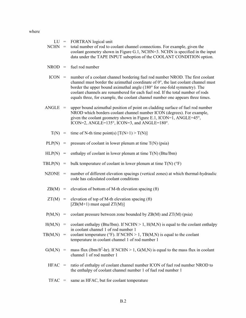
B.2

where LU = FORTRAN logical unit NCHN = total number of rod to coolant channel connections. For example, given the

coolant geometry shown in Figure G.1, NCHN=3. NCHN is specified in the input data under the TAPE INPUT suboption of the COOLANT CONDITION option.

NROD = fuel rod number ICON = number of a coolant channel bordering fuel rod number NROD. The first coolant

channel must border the azimuthal coordinate of 0°, the last coolant channel must border the upper bound aximuthal angle (180° for one-fold symmetry). The coolant channels are renumbered for each fuel rod. If the total number of rods equals three, for example, the coolant channel number one appears three times.

ANGLE = upper bound azimuthal position of point on cladding surface of fuel rod number

NROD which borders coolant channel number ICON (degrees). For example, given the coolant geometry shown in Figure E.1, ICON=1, ANGLE=45°, ICON=2, ANGLE=135°, ICON=3, and ANGLE=180°.

T(N) = time of N-th time point(s) [T(N+1) > T(N)] PLP(N) = pressure of coolant in lower plenum at time T(N) (psia) HLP(N) = enthalpy of coolant in lower plenum at time T(N) (Btu/lbm) TBLP(N) = bulk temperature of coolant in lower plenum at time T(N) (°F) NZONE = number of different elevation spacings (vertical zones) at which thermal-hydraulic

code has calculated coolant conditions ZB(M) = elevation of bottom of M-th elevation spacing (ft) ZT(M) = elevation of top of M-th elevation spacing (ft) [ZB(M+1) must equal ZT(M)] P(M,N) = coolant pressure between zone bounded by ZB(M) and ZT(M) (psia) H(M,N) = coolant enthalpy (Btu/lbm). If NCHN > 1, H(M,N) is equal to the coolant enthalpy

in coolant channel 1 of rod number 1 TB(M,N) = coolant temperature (°F). If NCHN > 1, TB(M,N) is equal to the coolant

temperature in coolant channel 1 of rod number 1 G(M,N) = mass flux (lbm/ft2-hr). If NCHN > 1, G(M,N) is equal to the mass flux in coolant

channel 1 of rod number 1 HFAC = ratio of enthalpy of coolant channel number ICON of fuel rod number NROD to

the enthalpy of coolant channel number 1 of fuel rod number 1 TFAC = same as HFAC, but for coolant temperature

B.3

GFAC = same as HFAC, but for mass flow

Figure B.1. Example Geometry for Input of Coolant Channel Data

PUP(N) = pressure in upper plenum (psia) HUP(N) = enthalpy in upper plenum (Btu/lbm) TBUP(N) = temperature in upper plenum (°F).

B.2 Heat Transfer Coefficient Option

If the heat option and tape2 suboption are specified in the $boundary input data block, the data set prescribing the fuel rod cooling must be created as follows:

DO 100 N = 1,NTSTEP

WRITE(LU)T(N)

DO 50 M = 1,NZONE

50 WRITE(LU)ZB(M),ZT(M),HTC(M,N)TB(M,N)P(M,N)

100 CONTINUE where HTC(M,N) = heat transfer coefficient in region of M-th elevation spacing at N-th time point

(Btu/hr-ft2-F).

The coolant temperature in the coolant condition data set must be such that Q(M,N) = HTC(M,N) (TCLAD - TB(M,N))

B.4

where Q(M,N) = surface heat flux (Btu/ft2-hr) TCLAD = cladding surface temperature (°F) HTC(M,N) = heat transfer coefficient (Btu/ft2-F-hr) TB(M,N) = coolant temperature for forced convection mode of heat transfer and saturation

temperature for boiling modes of heat transfer (°F).

The data set will be accessed by FoerN logical unit 4. The control statement for Fortran unit 4 must specify the location of the data set.

Appendix C –

Calculation of Cladding Surface Temperature

C.1

Appendix C: Calculation of Cladding Surface Temperature

The numerical solution of the heat conduction Equation (2.16) requires solving a set of tridiagonal equations. This set of equations is shown as follows:

N

Nm

N

mN

m

m

m

NN

NNN

dd

ddd

TT

TTT

bacbas

cbascba

cb

1

3

2

1

1

11

13

12

11

111

333

222

11

0'0

'0000

−+

+−

+

+

+

−−−

⋅⋅⋅

=

⋅⋅⋅

⋅

⋅⋅⋅⋅⋅⋅⋅⋅

(C.1) where an, bn, cn, and dn are terms of the heat conduction equation in finite difference form at

the n-th mesh point and where Tn

m+1 = temperature at n-th mesh point at time step m+1 n = number of mesh point at outer surface

The mesh point temperatures are solved by the Gaussian elimination method.

1

11

−

−+

−−

=nnn

nnnmn Eab

FadT

jmjj

mj FTET +−= +

++ 1

11

−−=−=

==

−−

−

)/()()/(

/,/

11

1

111111

jjjjjjj

jjjjj

EabFadFEabcE

bdFbcE for j = 2, 3, … n-1 (C.2)

The coefficients an, bn, and dn in the first equation of Equation (C.2) are derived from the energy balance equation for the half mesh interval bordering the outside surface. The continuous form of the energy balance equation for this half mesh interval is

VqA

rrrnP

n

ntTKA

tTVC

∆+−

∆−=

− ∂∂

−=∂∂

∆θ

ρ2

21 (C.3)

C.2

where all the terms in Equation (C.3) are defined below.

The finite difference form of Equation (C.3) is

n

nn

d

mmmn

mn

mn

nmn

P

mn

b

nPmn

a

n

VqATTr

KAT

rVC

Tr

KA

tVCT

r

KA

∆++−−∆

−

∆∆

=

∆+

∆∆

+∆

−

++−

−

+−+−

−

21

21

21

21

)(5.0)(5.0

5.05.0

11

111

θθρ

ρ

(C.4)

The complete expressions for the coefficients an, bn, and dn are then

r

KAa

nn ∆

−=

− 215.0

r

KA

tVCb

nPn ∆

+∆

∆=

− 215.0ρ

VqATT

r

KAT

rVCd mmm

nm

nm

nnm

nP

n ∆++−−∆

−

∆∆

= ++−

−21

21

)(5.0)(5.0

11 θθρ

)2/(22

1 rrA nn ∆−=− π

nn rA π2= (C.5)

)4/( 2rrrV n ∆−∆= π where K = thermal conductivity of material in half mesh interval bordering the surface Cp = specific heat of material in half mesh interval bordering the surface ρ = density of material in half mesh interval bordering the surface rn = radius to outside surface Δr = width of mesh interval bordering outside surface Δt = time step θm = surface heat flux at m-th time step Tn

m = surface temperature at m-th time step qm-1/2 = heat generation rate in half mesh interval bordering outside surface (heat

generation caused by cladding oxidation)

Because the coefficients an, bn, dn, En-1, and Fn-1 in Equation (C.2) do not contain temperature, the first equation of Equation (C.2) can be written as

C.3

11

11

++ =+ mmn BTA θ (C.6)

where

nnnn AEabA 5.0/)( 11 −−−=

∆−−−∆

∆−+

−=

−−−

n

mmn

mnn

mn

pnnn

m

A

VqTTaTVt

CFaA

B5.0

)(5.0 21

11

1

ρθ

(C.7)

As shown in Equation (C.2), the coefficients En-1 and Fn-1 are evaluated by forward reduction of Equation (C.1). So Equation (C.6) contains only Tn

m+1 and θm+1 as unknown quantities.

Empirically derived heat transfer correlations are available from which the surface heat flux due to convection can be calculated in terms of surface temperature, geometric parameters, and flow conditions. Also, the equation for radiation heat transfer from a surface to surrounding water is known. Thus, the total surface heat flux can be expressed by the equation

[ ]44111 )(),,( wm

nEAm

nim TTFFTGCf −+= +++ σθ (C.8)

where θm+1 = surface heat flux at time step m+1 f1 = function specifying rate at which heat is transferred from surface by convention

heat transfer during heat transfer mode i (These functions are defined in Section D.6 of Appendix D.)

i = number identification of convective heat transfer mode (nucleate boiling, film boiling, etc.)

C = set of parameters describing coolant conditions G = set of parameters describing geometry σ = Stefan-Boltzmann constant FA = configuration factor for radiation heat transfer FE = emissivity factor for radiation heat transfer TW = bulk temperature of water surrounding fuel rod surface

Equations (C.6) and (C.8) are two independent equations with unknowns Tnm+1 and Qm+1. Simultaneous

solution of the two equations yields the new surface temperature Tnm+1.

Appendix D –

Heat Transfer Correlations and Coolant Models

D.1

Appendix D: Heat Transfer Correlations and Coolant Models

The cladding-coolant heat transfer correlations used in FRAPTRAN are described in this appendix. The heat transfer correlations supply one of the equations required for calculation of the fuel rod surface temperature, as discussed in Section 2.2.1. Also described are the optional coolant enthalpy models and the calculation of coolant void fraction.

D.1 Heat Transfer and Critical Heat Flux Correlations

The correlations for heat transfer coefficient and critical heat flux have been selected based on their applicability to the range of conditions that are expected to be encountered in analyses with FRAPTRAN. Because the code is used for analysis of the response of a single fuel rod to postulated operational transients and design basis accidents, and to model fuel performance experiments, heat transfer models have been selected that are applicable to a wide range of relatively severe thermal-hydraulic conditions, particularly in the post-critical-heat-flux (CHF) regimes. The available correlations for determining the transition from nucleate boiling to film boiling (i.e., the CHF or departure from nucleate boiling [DNB]) are described in Section D.6.

The heat transfer correlations in FRAPTRAN cover the full range of the boiling curve, from single-phase forced convection to subcooled liquid through nucleate boiling to the critical heat flux point, on into transition and film boiling in the post-CHF heat transfer regimes, and finally to single-phase forced convection to superheated steam. The available heat transfer correlations for each regime are described in Section D.7. The code also includes a special set of correlations for the post-loss-of-coolant accident (LOCA) reflood transient, derived from the FLECHT tests, and this option is described in Section D.2.

D.2 Reflood Heat Transfer

The reflood heat transfer models available in FRAPTRAN-2.0 are based on work performed in two large-scale experimental programs simulating the reflood portion of loss-of-coolant accident conditions in representative PWR geometries. The earlier of the two is the PWR FLECHT (Full Length Emergency Cooling Heat Transfer)D1,D.2,D.3,D.4 program, which obtained data in test sections consisting of 7x7 and 10x10 arrays of electrically heated rods simulating a Westinghouse 15x15 fuel assembly. The second program, the Full Length Emergency Core Heat Transfer Separate Effects and Systems Effects Tests (FLECHT/SEASET) D5, D6, D7, D8, expanded the capabilities of the FLECHT facility to accommodate a test section of 161 rods, representing a portion of the array of Westinghouse 17x17 fuel assemblies within a PWR core.

A detailed heat transfer model was developed and documented for the original FLECHT data set (see Ref. D.4). This model was implemented in FRAPTRAN, and can be accessed as the ‘15x15’ geometry model option (see Appendix A, input instructions for group ‘reflood’). A separate detailed heat transfer model was developed for the FLECHT/SEASET data (see Appendix I of Ref. D.7), and is available in FRAPTRAN as the ‘frap-t4’ option in input group ‘reflood’, but this model has not been validated in FRAPTRAN, and is not recommended for general use (see Appendix A).

The original FLECHT model was later generalized to include the FLECHT/SEASET data, with additional minor modifications to scale the test data to in-reactor conditions, for application to post-LOCA reflood calculations. This generalized FLECHT correlation is the default option for reflood heat transfer modeling with FRAPTRAN, and is used to calculate the heat transfer coefficient at the cladding surface during the reflood phase of a LOCA.

D.2

The formulation of the generalized FLECHT heat transfer model in FRAPTRAN1.5 for post-LOCA reflood is unchanged from the previous version of the code, FRAPTRAN 1.4. The heat transfer coefficient is a function of flooding rate, cladding temperature at the start of flooding, fuel rod power at the start of flooding, flooding water temperature, vessel pressure, elevation, and time. The ranges of these variables for which the FLECHT correlation is applicable are shown in Table D.7. The FLECHT correlation divides the reflood heat transfer into four time periods and has a different heat transfer correlation for each period. Using the definitions shown in Table D.8, the four regimes are described below.

D.2.1 Period of Radiation Only

Only heat transfer due to radiation is modeled during 0 > t ≥ t1, with the heat transfer coefficient being calculated by the expression

[ ])0025.0exp(1 20 thhh −−∆+= (D.1)

where

)30(2.0max

1 501)25.1exp()465.0exp()0034.0exp(274

−−+′−−−

= Pininit QVTt

°≤

°>

−

−−′=

FTif

FTifFTQhinit

initinit

700,0

700,435

700exp167.3 max0

72

2 5011

−+−

+= ZFFF

inVF −+

+= 22 5017.03.0

)100(0397.0 max −′=∆ initTQh (D.2)

D.2.2 Period I

During Period I, the flow develops from the radiation dominated prereflood condition to single phase steam flow, to dispersed flow, and finally to unstable film boiling. However, if the flooding rate is less than 3 in./s, unstable film boiling does not develop. The heat transfer coefficient during this period changes from a low value due to radiation to a relatively high value due to unstable film boiling (high flooding rates) or dispersed flow (low flooding rates). The time range of Period I is

tt <1 (D.3)

and

2qq tt < (D.4)

D.3

where the variables in the expression for time range are defined as

1

1

6tt

tttq

q −−

= (D.5)

where

{ }

{ } { }

++⋅

++

⋅−−+

⋅

−+⋅−−+

−′

⋅

−−+

−+−+

⋅−∆−

=

−− pV

initinit

inin

tq

in

in

insub

q

in

TTpVV

Q

VpVp

VT

t

1.05667.02

31.1

5.1max

23

23

50132.01

5015.01

))0025.0exp(05.10000588.01()000037.0exp(5.01)exp(8.2)/28.3(

)667.0207.1(

)49.0exp(000037.0exp(3.17

)111.0exp(3.1)000037.0exp(5.01

)667.0exp(1)0107.0exp(

39.986

(D.6)

( ))0368.0exp(115.0))192.0exp(1(62.0 22

ZZZtq −−−−=

The heat transfer coefficient during Period I is calculated using the correlation

[ ]

( ){ }

+

−−−−−

⋅−−−−

⋅

−−−−+

−−−=

−910

2

2

2

2112

2

21

21001

824.3588.0exp)exp()4.0exp(21.21

)exp(9.0)exp(1

10exp110exp1

q

q

tt

inin ZuuV

XXX

XXXhh

XXXhh

(D.7)

where

°≤−−∆

°>−−∆+

−−−′

=FTifth

FTifthTQh

init

initinit

700)),0025.0exp(1(

700)),0025.0exp(1(435

700exp167.3

21

21max

1

[ ] { }[ ]162

2 2))8(0000272.000075.0(exp1)0166.0exp(37.416.17 ftfVTX qinsub −+−−⋅∆−+=

[ ][ ] [ ] [ ])25/exp(12exp(18)2.0exp(1

))0011.0exp(034.0)0383.0exp(1()00303.022(7.35092.1644.2

)

21.4max12

BVVPPPZQh

inin −−⋅−−+−−⋅−−−−⋅−++′+=

D.4

[ ] { }[ ]2

62 1

16

2

())8(0000272.00075.0(exp1)0166.0exp(37.416.17

f

qqinsub ttt

ttfVTX

−−

⋅−+−−⋅∆−+=

2

11

32

2

9

= + ff

q

q

ttf

u

51 455.0436.0 ff +=

52 455.0564.0 ff +=

)67.1688.0exp(8.48.23 inVf −−=

{ })651.0)01.3exp(28.10041.1026.0(exp1 max4 −′−++−−= QVPf in

inV

QQf 25max

max5 50124.1

−+′−

+′=

{ } 350)10(0001.1200010005.0 21

626 +

+−+−= initinitinit TTTf

D.2.3 Period II

During this period, the flow pattern has fully developed to a quasi-steady state of either unstable film boiling (high flooding rate) or dispersed flow (low flooding rate), and the heat transfer coefficient reaches a plateau with a rather slow increase. The time range of Period II is

32 qqq ttt << (D.8)

where the new variable in the expression for time range is defined as

( )( ) 262 )10(77.2exp(26.0)0421.0exp(154.0)205.0exp(155.13 initq TZZZt −−+−−−−= (D.9)

The heat transfer coefficient during Period II is computed by the equation

[ ]

[ ]

−×−

+−+−++=

−

2

33

26

24

33

22

212

25.2exp1077.2exp60

)38.6exp()(

yy

yyT

yybybybybhh

init

(D.10)

where

( )[ ])exp(9.0)exp(1 2222122 XXXhh −−−−=

D.5

{ }[ ] { }[ ]

{ }[ ][ ][ ][ ])3025851.20986123.18503.0exp(1)1(2.01

)25/exp(304.0696.00238.0exp1)0304881(95.0exp1)4exp(1650682

24

1

++−+−+

⋅−+∆−−⋅−−−⋅−−−=

ZZfBT

VZZb

sub

in

2qq tty −= (D.11)

{ }[ ][ ]

[ ][ ])25/exp(1)5.2/exp(19.21))0227.0exp(1(33.1)5.3(2exp14.02

BVPXZD

in −−−−−−−−−−−=

)7.3exp()7.3(55.2 23 ZZb −−=

)036.0exp()exp(5.87 24 subinin TVVb ∆−−=

0,4 23 ==< bbZif

D.2.4 Period III

During this period, the flow pattern changes to stable film boiling and the heat transfer coefficient increases rapidly as the quench front approaches. The time range of Period III is

qq tt <3

(D.12)

where tq is the time of quenching. The heat transfer coefficient during Period III is calculated by the expression

)(33 qq ttChh −+= (D.13)

where

[ ])38.6exp()( 3234

333

232

23123 yybybybybhh −+−++=

[ ] 41)00625.0exp(1420 fbC −−= (D.14)

233 qq tty −=

D.2.5 Modification for Low Flooding Rates

The heat transfer coefficients for Periods I, II, and III given above are based on the original FLECHT tests. Later tests performed at low flooding rates showed that a modification was necessary to best match the data. This modification is accomplished by multiplying the heat transfer coefficients for Periods I, II, and III by a factor f where

D.6

87 fff = (D.15)

and

( )( )162301022.0978.07 tttt qqq

f −−++=

78 5011

−+−

+= Za

afff (D.16)

inV

bba

fff −+−

+= 25011

[ ])5.1exp(17.03.0 qb tf −−+=

D.2.6 Modification for Variable Flooding Rates and Variable Rod Length

The variable t in the FLECHT heat transfer correlation is the time after the start of flooding as adjusted for variable flooding rate. The adjustment of time is made according to the equation

−−+=∫

AAin

t

in

A ttV

dttVZtt

A

)(

)()386.0214.0( 0 (D.17)

where t = adjusted time (s) tA = actual time since start of flooding (s) Z = equivalent FLECHT elevation (ft) Vin(t) = flooding rate at time t (in./s)

The integral-of-power methodD.9 is used to calculate the elevation in the FLECHT facility that is equivalent to a given elevation in a nuclear reactor. By using the equivalent FLECHT elevation in the FLECHT correlation, the heat transfer coefficient at the given elevation in the nuclear reactor is calculated. The equation used to calculate the equivalent FLECHT elevation is

dZZPFFdZZP

Z

LL

FZ

F ∫∫ =21

00

)()( (D.18)

where PF(Z) = normalized power of FLECHT rod at elevation Z PL(Z) = normalized power of nuclear rod at elevation Z FF = axial power peaking factor for FLECHT rod = 1.66 FL = axial power peaking factor for nuclear rod (specified by code input)

D.7

Z2 = elevation on nuclear fuel rods Z1 = elevation on FLECHT rods that is equivalent to elevation Z2 on nuclear fuel rods

The procedure for solving for the equivalent FLECHT elevation Z1 that corresponds with the nuclear reactor elevation Z2 is

1. Store in computer memory a table of the integral of normalized FLECHT power versus elevation.

2. Numerically integrate the normalized power of the nuclear rod from elevation zero to elevation Z2.

3. By interpolation in the table of Step 1, find the FLECHT elevation that has the same integral of power as the nuclear reactor at elevation Z2.

D.3 Influence of Rod Bowing on Critical Heat Flux

The calculation of critical heat flux reduction due to fuel rod bowing is a user option in FRAPTRAN. If this option is used, both critical heat flux and fuel rod power are calculated according to the amount of fuel rod bowing. The reductions are calculated by empirical correlations. The correlations for critical heat flux reduction are

Thr

ThrBCHFCHF W

WZWFZf−

−=∆

1)()(

ThrCHF WZWifZf ≤=∆ )(0)( (D.19)

)()(1)( ZqZfZq CHFCHFCHFR ∆−= where Δf(Z) = fractional decrease in critical heat flux due to fuel rod bowing at elevation Z qCHFR = reduced critical heat flux qCHF = critical heat flux in absence of fuel rod bowing W(Z) = amount of fuel rod bowing (fraction of bowing required to contact adjacent fuel

rod, 0 = no bowing, 1 = maximum possible bowing) WThr = maximum amount of bowing which can occur without an effect on CHF (fraction

of maximum bowing possible) (this quantity is specified by user input). FBCHF = multiplication factor specified by user input

The reduction in fuel rod power due to bowing is calculated by the equation

[ ]PZWZWPr ))(84.2)(94.0(01.01 2−+= (D.20)

)3.0)(( ≤= ZWforPPr where Pr = power reduced to account for fuel rod bowing P = power in absence of fuel rod bowing

D.8

D.4 Void Fraction

The void fraction of the coolant is calculated by the equation

gf

g

XVVXXV

+−=

γα

)1( (D.21)

where α = void fraction X = coolant quality Vf = specific volume of saturated liquid Vg = specific volume of saturated gas γ = slip velocity ratio

The slip velocity ratio for void fraction calculations is always assumed to be 1.0 (homogeneous flow).

D.5 Coolant Enthalpy Model

The coolant enthalpy is calculated by a one-dimensional transient fluid flow model D.10. The model is given as input information the coolant enthalpy and mass flux at the bottom of the fuel rods and the elevation averaged coolant pressure. The input information can vary with time. The model also receives the FRAPTRAN calculated cladding surface heat flux. The heat flux can vary with time and elevation. The coolant enthalpy model then calculates the coolant enthalpy, which varies with time and elevation.

The model includes an energy conservation equation and a mass conservation equation. The coolant pressure is assumed to be spatially uniform and to change slowly with time so that the spatial and transient pressure terms are omitted from the energy equation. Thus, sonic effects are ignored. The model assumes homogeneous two-phase flow and a flow channel with a constant cross-sectional area.

The energy and mass conservation equations are

)(1 rqLz

HGt

H+=

∂∂

+∂

∂ ϕρ (D.22)

0=∂∂

+∂∂

zG

tρ (D.23)

where ρ = coolant density (kg/m3) G = coolant mass flux (kg/m2∙s) H = coolant enthalpy (J/kg) (φ+rq)/L = volumetric heat addition to coolant (J/m3∙s) L = flow area per unit transfer surface are per unit axial length (m) φ = surface heat flux (J/m2∙s) q = heat generation rate/area (J/m2-s) r = fraction of heat generated directly in the coolant by neutrons and gamma rays t = time (s) z = axial elevation (m)

D.9

Assuming constant pressure, coolant conditions are considered a function of enthalpy only so that

Ht

Ht

andH∂∂

⋅∂

∂=

∂∂

=ρρρρ )( (D.24)

where density is evaluated at a reference pressure. By combining Equations (D.22), (D.23), and (D.24), a relation can be established between the axial mass flux distribution and axial enthalpy distribution:

∂∂

−+∂∂

−=∂∂

⋅∂

∂−=

∂∂

−=∂∂

zHGrq

LHHtH

tzG )(11 ϕρ

ρρρ

(D.25)

The numerical solution for the local coolant enthalpy is given by the finite difference form of Equation (D.24) with forward difference in time and averaged between spatial nodes. The equation is

)1(

211

)(2

12

1

21

21

21

1111

1

−−

−+

−

−+−−

−

+

∆+

+

−−−=

jj

j

j

jjjjj

QtHHHH

αραα

(D.26)

where

jj

jj z

tG∆

∆=

−

+−

−

21

21

21

1

ρα

)(21

121

−− += jjj ρρρ

)(21 1

111

21

+−

++− +=

jjj GGG

)(21)(

21

1121

−−− +++= jjjjj rqrq

LLQ ϕϕ

j = FRAPTRAN axial node number (see Figure D.2) = time step number 1−−=∆ jjj zzz

1−−=∆ ttt .

The numerical solution for the mass flux at the midpoint between axial nodes j and j-1 at the new time step is given by the finite difference form of Equation D.25. The equation is

2

12

22

21

21

21

21

21

211

11

−

∆

∂∂

+−

+=

−

−−−

−

−+−

+

j

jjjj

j

jjj A

zQH

AA

GG

ρρ

(D.27)

where

2

12

12

1

1

−−− ∆=

jjj dH

dHA ρρ

D.10

1

1

21 −

−

− −−

jj

jj

j HHdHd ρρρ

1−−=∆ jj HHH .

Gjℓ+1 is calculated using Equation (D.27) before Hj

ℓ+1 is calculated with Equation D.26. After the coolant enthalpy at the new time step has been calculated, the coolant density at the new time step is determined from the equation of state for water.

In summary, coolant inlet enthalpy and mass flux are input to define conditions at node zero. The mass fluxes for the remaining nodes are calculated from Equation (D.28) using values for heat flux, enthalpy, and density calculated in the previous time step or iteration. The enthalpy is then updated using Equation (D.26), and a corresponding density is calculated from the fluid property relationships. Using the fluid conditions in the heat transfer correlations, a new heat flux is calculated, and the process is repeated.

If the time step is less than the minimum time for a drop of coolant to pass between any two axial nodes, the solution scheme is stable. This criterion is given by the equation

min2

1

∆≤∆

+

j

j

vz

t (D.28)

where

21+jv is the velocity of coolant at midpoint between axial nodes j and j + 1 (m/s).

The coolant quality and temperature are computed by the following equations:

)),(()(

0)()()(

.1PzhzT

zXPHzh

Case

ii

i

Fi

θ==

≤ (D.29)

)()()()()()()(

)()()(

.2

PTzTPHPHPHzHzX

PHzHPH

Case

si

FG

Fii

GiF

=−−

=

≤≤

(D.30)

)),(()(

1)()()(

.3PzHzT

zXPHzH

Case

ii

i

Gi

θ==

≥ (D.31)

where Xi = quality of coolant in flow channel i at distance z from flow inlet Ti(z) = temperature of coolant in flow channel i at distance z from flow inlet (K) HF(P) = enthalpy (J/kg) of saturated liquid at coolant pressure P (N/m2) HG(P) = enthalpy (J/kg) of saturated gas at coolant pressure P Ts(P) = saturation temperature (K) at coolant pressure P

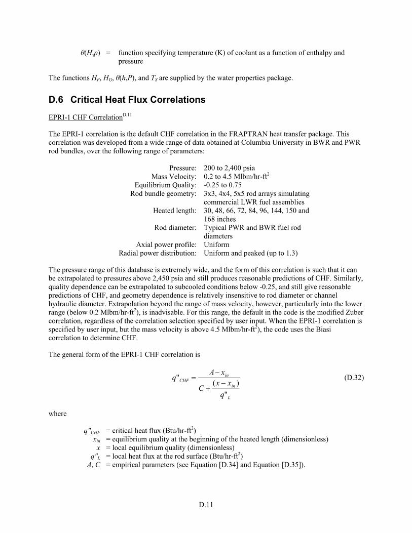
D.11

θ(H,p) = function specifying temperature (K) of coolant as a function of enthalpy and pressure

The functions HF, HG, θ(h,P), and TS are supplied by the water properties package.

D.6 Critical Heat Flux Correlations

EPRI-1 CHF CorrelationD.11

The EPRI-1 correlation is the default CHF correlation in the FRAPTRAN heat transfer package. This correlation was developed from a wide range of data obtained at Columbia University in BWR and PWR rod bundles, over the following range of parameters:

Pressure: 200 to 2,400 psia Mass Velocity: 0.2 to 4.5 Mlbm/hr-ft2

Equilibrium Quality: -0.25 to 0.75 Rod bundle geometry: 3x3, 4x4, 5x5 rod arrays simulating

commercial LWR fuel assemblies Heated length: 30, 48, 66, 72, 84, 96, 144, 150 and

168 inches Rod diameter: Typical PWR and BWR fuel rod

diameters Axial power profile: Uniform

Radial power distribution: Uniform and peaked (up to 1.3)

The pressure range of this database is extremely wide, and the form of this correlation is such that it can be extrapolated to pressures above 2,450 psia and still produces reasonable predictions of CHF. Similarly, quality dependence can be extrapolated to subcooled conditions below -0.25, and still give reasonable predictions of CHF, and geometry dependence is relatively insensitive to rod diameter or channel hydraulic diameter. Extrapolation beyond the range of mass velocity, however, particularly into the lower range (below 0.2 Mlbm/hr-ft2), is inadvisable. For this range, the default in the code is the modified Zuber correlation, regardless of the correlation selection specified by user input. When the EPRI-1 correlation is specified by user input, but the mass velocity is above 4.5 Mlbm/hr-ft2), the code uses the Biasi correlation to determine CHF.

The general form of the EPRI-1 CHF correlation is

L

in

inCHF

qxx

C

xAq

")(

"−

+

−= (D.32)

where q″CHF = critical heat flux (Btu/hr-ft2) xin = equilibrium quality at the beginning of the heated length (dimensionless) x = local equilibrium quality (dimensionless) q″L = local heat flux at the rod surface (Btu/hr-ft2) A, C = empirical parameters (see Equation [D.34] and Equation [D.35]).

D.12

The equilibrium quality is defined as

fg

f

hhh

x−

= (D.33)

where h = bulk fluid enthalpy (Btu/lbm) hf = saturated liquid enthalpy (Btu/lbm) hfg = latent heat of vaporization (Btu/lbm)

Parameters A and C are optimized statistical fits relating CHF to test conditions of pressure and mass velocity, and have the form

rPcccr GPcA 752

1+= (D.34)

rPcccr GPcC 864

3+= (D.35)

where Pr = critical pressure ratio, P/Pcrit

where P = system pressure (psia) Pcrit = critical pressure (3,208.2 psia for water)

G = local mass velocity (Mlbm/hr-ft2) cn = optimized constants from statistical fit to data (see Table D.1)

Table D.1. Optimized Constants for EPRI-1 CHF Correlation

c1 0.5328 c2 0.1212 c3 1.6151 c4 1.4066 c5 -0.3040 c6 0.4843 c7 -0.3285 c8 -2.0749

The base correlation (Equation (D.32)) can be modified with three optional correction factors:

1. a two-part cold wall correction for corner-peaked bundles modeled with subchannels (primarily applicable to BWR fuel assemblies)

2. a grid spacer correction factor for rod bundles with relatively high-loss grid designs (primarily applicable to fuel assemblies with mixing vane grids)

3. a non-uniform axial power correction factor

D.13

All of these options can be selected by user input. However, the default is to use only the base correlation.

The cold wall correction is applied by means of the following modifications to the critical heat flux defined in Equation (D.32):

L

inC

inACHF

qxx

CF

xFAq

")(

"−

+

−= (D.36)

The cold wall correction factors are defined as

1.0

1.0

183.1000.1

GFGF

C

A

==

The grid spacer correction is applied in a similar manner, as

L

ing

inCHF

qxx

CF

xAq

")(

"−

+

−= (D.37)

The grid spacer correction factor is defined as

gg CF 3.03.1 −=

where Cg is the form loss coefficient for grid (dimensionless).

The non-uniform axial power correction is applied in the same way, as

L

innu

inCHF

qxx

CF

xAq

")(

"−

+

−= (D.38)

The non-uniform axial power correction factor is defined as

)1()1(0.1

GYFnu +

−+=

where Y is Bowring’s non-uniform axial power factor (see Equation [D.48]).

Bowring’s Mixed Flow Cluster CHF CorrelationD.12

The CHF correlation developed by Bowring for mixed flow clusters can be specified by user input. This correlation was developed for application to thermal-hydraulic analysis of blowdown transients modeled with RELAP-UK, and is designed with the assumption that the local fuel assembly subchannels are modeled as a single assembly-averaged flow channel. This correlation is not designed for detailed subchannel analysis of the rod array. (For such applications, the EPRI-1 correlation is the recommended option.)

D.14

Bowring’s correlation was developed from a very large database with test geometries representing rod clusters in pressure tube reactors, as well as test assemblies modeling BWR and PWR rod bundles. This correlation’s database includes the following range of parameters;


Hydraulic diameter: 0.3 to 1.4 inches (based on heated perimeter) Heated length: 60 to 180 inches Rod diameter: Typical PWR and BWR fuel rod diameters

Axial power profile: 1.0 to 1.38 peak-to-average axial flux ratio Radial power distribution: 1.0 to 1.32 peak-to-average rod power ratio

The pressure range of this database is extremely wide, and dependence on this parameter is such that the correlation can generally be extrapolated to pressures above 2,250 psia and still produces reasonable predictions of CHF. Similarly, geometry dependence is relatively insensitive to rod diameter or channel hydraulic diameter. Extrapolation beyond the range of mass velocity of the correlation’s database, however, particularly into the lower range (below 0.04 Mlbm/hr-ft2), is inadvisable. For this range, the default in the code is the modified Zuber correlation, regardless of the correlation specified by user input.

The general form of Bowring’s mixed cluster correlation is

YZChBA

q inCHF +

∆−=" (D.39)

where q″CHF = critical heat flux (Btu/hr-ft2) Δhin = enthalpy subcooling (Btu/lbm) at the inlet, (hf – hin)

where hf = saturated liquid enthalpy (Btu/lbm)

hin = fluid enthalpy (Btu/lbm) at the inlet Z = axial distance from beginning of heated length (inches) Y = non-uniform axial heat flux correction factor (see Equation [D.47]) A, B, C = empirical parameters (see Equation [D.40] through Equation [D.44] for parameter

A, Equation [D.45] for parameter B, and Equation [D.46] for parameter C), based on data obtained in pressure tube geometries with subcooled inlet conditions

The empirical parameter A of this correlation is a function of the flow rate, the system pressure and the geometry (through the hydraulic diameter terms), and is defined as follows:

−+

+

=

)]1)/(8.0(1[)(52.1

1

2.242

3.12

21

hePh

eP

e

DDFGDFGDF

DGFA (D.40)

where G = mass velocity (lbm/hr-ft2) De = channel hydraulic diameter, based on wetted perimeter (ft) Dh = channel hydraulic diameter, based on heated perimeter (ft)

D.15

FP = radial peaking (ratio of peak rod power to average rod power) F1, F2 = empirical parameters (see Equation [D.41] and Equation [D.42])

The parameters F1 and F2 in Equation (D.40) are statistically fitted functions of pressure, and have the form

[ ]22

1 )47.01(04.00.1 TT PPF +−= (D.41)

>+−≤<−+

≤+=

psiaPforPPpsiaPforPP

psiaPforPF

TT

TT

T

650)135.032.0()2.3(650415556.1959.1424.0

41525.145.02

2 (D.42)

where PT is reduced pressure; 0.001 P, where P is the system pressure in psia.

The formulation in Equation (D.40) for parameter A is applicable to PTR, BWR, and PWR geometries when the pressure is below 1,250 psia. When the system pressure is above 1,250 psia, however, this parameter requires additional terms, as follows:

)()001.0250.2( 212 AAPAA −−+= (D.43) where A1 = A from Equation (D.40), evaluated at P = 1,250 psia A2 = correlation parameter (see Equation [D.44])

The high-pressure term for parameter A is a function of mass velocity and geometry, and is defined as

GDG

GA e

++=

1.05.9

0.182 (D.44)

where G = mass velocity (lbm/hr-ft2) De = channel hydraulic diameter, based on wetted perimeter (ft)

Correlation parameter B is a function of the mass velocity and channel hydraulic diameter, and is defined as

Ge eDGB 2.025.0 −= (D.45)

where G = mass velocity (lbm/hr-ft2) De = channel hydraulic diameter, based on wetted perimeter (ft)

Correlation parameter C contains the axial power shape correction factor, and is of the form

D.16

+−

+=110.160 27.057.0

GYGDC h (D.46)

where G = mass velocity (lbm/hr-ft2) Dh = channel hydraulic diameter, based on heated perimeter (ft)

The parameter Y is the non-uniform axial heat flux correction factor for this correlation, and is defined as

ZZq

dzzqY

Z

)("

)("0∫= (D.47)

where )(" zq = radially averaged axial heat flux at axial location z (Btu/hr-ft2) Z = axial distance from beginning of heated length (inches)

The integral in Equation (D.47) is adapted to the discrete noding of a computer model by converting the continuous integration function to a summation over the axial noding steps, as

JJ

J

jjj

Z

Xq

xq

ZZq

dzzq"

2

"

0

)("

)(" ∑∫ =

∆≅ (D.48)

where "

jq = radially averaged axial heat flux at node j (Btu/hr-ft2) XJ = axial distance from beginning of heated length to node J (inches) Δxj = length of axial node j (inches) j = axial node index counter J = index of axial node corresponding to axial distance Z

MacBeth’s CHF CorrelationD.13

The CHF correlation developed by MacBeth and Thompson can be specified by user input. This correlation was developed using a database consisting of a compilation of a large amount of CHF data from a wide variety of sources. This data consisted entirely of uniformly heated round tubes with vertical upflow. The database includes the following range of parameters:

D.17


Hydraulic diameter: 0.04 to 1.475 inches Heated length: 1.0 to 144 inches

Axial power profile: uniform

Although the database of this correlation consists entirely of burnout tests in round tubes, the correlation has been successfully extrapolated to CHF in annuli and rod bundles at low pressure. For pressure conditions outside the range of the database, or mass velocities above 13.7 Mlbm/hr-ft2, the CHF correlation selection logic in FRAPTRAN defaults to the Biasi correlation. For mass velocity values below the extremely low lower bound of the database, the code defaults to the modified Zuber correlation.

The MacBeth correlation is constructed with two essentially separate functions, one applicable to CHF for relatively low flow conditions, and one for high flow conditions. At low flow conditions, the relationship between mass velocity and critical heat flux is approximately linear, and is essentially independent of pressure. For these conditions, the correlation defines the critical heat flux as

)1(10

00633.0"51.0

61.0

) xGDhq efgvelocitylowCHF −

= − (D.49)

where velocitylowCHFq )" = critical heat flux (Btu/hr-ft2) in low velocity region De = channel hydraulic diameter, based on wetted perimeter (ft) hfg = latent heat of vaporization (Btu/lbm) G = mass velocity (lbm/hr-ft2) x = equilibrium quality

For high flow conditions, the correlation defines the critical heat flux as a somewhat more complex function of mass velocity, equilibrium quality, and geometry, with a strong dependence on pressure. The form of the correlation in this region is

−=

CxhGDA

q fgevelocityhighCHF

)10/(25.0"

6

) (D.50)

where velocityhighCHFq )" = critical heat flux (Btu/hr-ft2) in high velocity region De = channel hydraulic diameter, based on wetted perimeter (ft) hfg = latent heat of vaporization (Btu/lbm) G = mass velocity (lbm/hr-ft2) x = equilibrium quality A, C = empirical parameters (see Equation [D.51] and Equation [D.52])

The empirical parameters A and C were defined using statistical optimization for two overlapping sets of data. The first data set consisted of 1,344 test points, over the following ranges of conditions:

D.18



The parameters A and C for this data set are formulated as

5

4

2

1

63

60

10

10y

ye

yy

e

GDyC

GDyA

=

=

(D.51)

where De = channel hydraulic diameter, based on wetted perimeter (ft) G = mass velocity (lbm/hr-ft2) yn = empirical coefficients (see Table D.2)

Table D.2. Coefficients for MacBeth’s 6-coefficient Model

Reference Pressure

(psia)

Fitted Coefficients

y0 y1 y2 y3 y4 y5 250 106.5 0.847 0.677 60.3 1.4 0.937 530 123.5 0.834 0.408 78.8 1.4 0.737 1,000 124.5 0.913 0.376 118 1.4 0.555 1,570 59.9 0.873 0.12 82.7 1.4 0.096 2,000 67.5 1.13 0.535 108 1.4 0.343 2,700 1.3 -0.05 1.02 103 1.4 0.529

The second data set expanded the number of test points by 232, to 1,576, to create the complete database of the correlation. The additional tests expanded the database to encompass the following ranges of conditions:



The parameters A and C for this data set are formulated as

+

++

=

+

++

=

611610966

6564360

10100.1

10

10100.1

108

7

2

1

GDyGyDyGDyC

GDyGyDyGDyA

ee

yy

e

ee

yy

e

(D.52)

D.19

where De = channel hydraulic diameter, based on wetted perimeter (ft) G = mass velocity (lbm/hr-ft2) yn = empirical coefficients (see Table D.3)

Table D.3. Coefficients for MacBeth’s 12-coefficient Model

Coefficient Reference Pressure (psia)

560 1,000 1,550 2,000 y0 237 114 36 65.5 y1 1.2 0.811 0.509 1.19 y2 0.425 0.221 -0.109 0.376 y3 -0.94 -0.128 -0.19 -0.577 y4 -0.0324 0.0274 0.024 0.22 y5 0.111 -0.0667 0.463 -0.373 y6 19.3 127 41.7 17.1 y7 0.959 1.32 0.953 1.18 y8 0.831 0.411 0.0191 -0.456 y9 2.61 -0.274 0.231 -1.53 y10 -0.0578 -0.0397 0.0767 2.75 y11 0.124 -0.0221 0.117 2.24

Modified Zuber CorrelationD.13, D.14

The modified Zuber correlation is included in the critical heat flux correlation selection option in FRAPTRAN, and can be selected by user input. This correlation was developed for critical heat flux calculations in LWRs in severe accident conditions and is applicable to very low flow conditions. The correlation is based on pool boiling critical heat flux hydrodynamics, and is formulated in terms of local fluid conditions, which makes it essentially independent of pressure. It was originally formulated for very high void fraction (above 96 percent), but modifications have been developed4 that make the range of applicability essentially independent of void fraction. This was done to make the correlation applicable to inverted annular film boiling, which can include conditions where the bulk fluid is subcooled.

The modified Zuber correlation is the default selection in the code for all cases where the mass velocity is below 0.2 Mlbm/hr-ft2 or the void fraction is above 80 percent. The general form of the correlation is as follows:

( )25.0)(1309.0" gfcgfgsubcGCHF gghFFq ρρσρ −= (D.53) where

4 Based on modifications to the Zuber correlation in the JAERI code NSR-77.

D.20

hfg = latent heat of vaporization (Btu/lbm) ρg = saturated vapor density (lbm/ft3) ρf = saturated liquid density (lbm/ft3) σ = surface tension (lbf/ft) g = acceleration of gravity (32.2 ft/s2) gc = 32.2 lbm-ft/lbf-s2 – force to mass conversion constant for EU FG = correction factor for extended void fraction range (see Equation [D.54]) Fsubc = correction factor for bulk subcooled fluid conditions (see Equation [D.55])

The correction factor to generalize the void fraction range of the correlation is defined as

)1(90.0 α−=GF (D.54)

where α is local void fraction (dimensionless).

The correction factor for bulk subcooled conditions is

−

+=

fg

bsatpf

g

fsubc h

TTcF

)(065.00.1

8.0

ρρ

(D.55)

where ρg = saturated vapor density (lbm/ft3) ρf = saturated liquid density (lbm/ft3) cpf = specific heat of saturated liquid (Btu/lbm-°F) hfg = latent heat of vaporization (Btu/lbm) Tsat = saturation temperature (°F) Tb = bulk fluid temperature (°F)

Biasi CorrelationD.15

The Biasi correlation is included in the critical heat flux correlation selection option in FRAPTRAN, and can be selected by user input. This correlation was developed for critical heat flux calculations in LWRs in severe accident conditions and is applicable to very wide range of conditions. The Biasi correlation is the automatic default in the code for conditions where the system pressure is below the pressure range of the user-selected correlation, or the mass velocity is above the user-selected correlation’s mass velocity range. However, if the void fraction is above 80 percent, the correlation selection defaults to the modified Zuber correlation, no matter what the flow rate or pressure, and regardless of which correlation has been selected by user input.

The Biasi correlation was derived in metric units, and has two separate formulations for the critical heat flux. The critical heat flux is defined as

)","max(" 21 chfchfCHF qqq =

The first component is defined as

( ) ne

bP

bchf DxGFGbq −−= 22

11" (D.56)

D.21

where G = mass velocity (g/s-cm2) FP = pressure-dependent empirical factor (see Equation (D.57)) x = equilibrium quality (dimensionless) De = channel hydraulic diameter, based on wetted perimeter (cm) b1, b2, n = empirical parameters

The pressure-dependent empirical factor FP is defined as

PbP ePbbF 5

43 += (D.57) where P = pressure (bar) b3, b4, b5 = empirical coefficients n = empirical coefficient on hydraulic diameter (see Equation (D.60))

The second component of the critical heat flux is defined as

( ) neH

cchf DxFGcq −−= )1(" 2

12 (D.58) where G = mass velocity (g/s-cm2) FH = pressure-dependent empirical factor (see Equation (D.59)) x = equilibrium quality (dimensionless) De = channel hydraulic diameter, based on wetted perimeter (cm) c1, c2 = empirical coefficients n = empirical coefficient on hydraulic diameter (see Equation (D.60))

The pressure-dependent empirical factor FH is defined as

+

++= 27

643

5

PcPc

ePccF PcH (D.59)

where P = pressure (bar) De = channel hydraulic diameter, based on wetted perimeter (cm) cn = empirical coefficients

The coefficient n on the hydraulic diameter in Equation (D.56) and Equation (D.58) is defined as follows:

≥<

=0.14.00.16.0

e

e

DifDif

n (D.60)

D.22

D.7 Heat Transfer Coefficient Correlations

Heat transfer correlations are empirical models developed to quantify the rate of energy exchange between a solid surface and a fluid flowing over it. Heat transfer correlations are expressed as a coefficient relating the surface heat flux to the temperature difference between the surface and the fluid:

)(" fluidw TThq −= (D.61) where q″ = surface heat flux, Btu/hr-ft2 (W/m2) Tw = wall surface temperature, °F (K) Tfluid = fluid temperature, °F (K) H = heat transfer coefficient, Btu/hr-ft2-°F (W/m2-K)

This relationship is a constitutive model based on empirical observation, not an expression of a law of nature. It is a convenient simplification of an extensive array of physical phenomena that influence the rate of heat transfer from a surface, which can include the thermodynamic properties of the flowing fluid, the fluid dynamic forces in the boundary layer, the effects of phase change (for boiling flow), and the geometry of the heated surface. There is no generic formulation for a heat transfer coefficient correlation that satisfies the above relationship for all conditions. Specific formulations for any particular application must be derived from experimental data.

For forced convection heat transfer, the general behavior of this relationship can be broadly divided into five regions, or modes, which are differentiated by the basic heat transfer behavior within each region. These are single-phase forced convection to liquid (Mode 1), nucleate boiling (Mode 2 for subcooled boiling and Mode 3 for saturated boiling), post-CHF transition boiling (Mode 4), post-CHF film boiling (Mode 5), and single-phase forced convection to vapor (Mode 8). (Modes 6 and 9, previously differentiated in FRAPTRAN, have been eliminated by introducing correlations with expanded ranges and more general applicability in the post-CHF regimes.) Figure D.1 illustrates the relationship between wall superheat and heat flux for the full range of regimes, and shows the typical shape of the boiling curve from single-phase liquid to single-phase vapor convection.

Additional Modes are defined in FRAPTRAN to cover the full range of flow conditions that can be encountered in severe transients, which do not always remain in the forced convection heat transfer regime. These are Mod 7 – low flow conditions, defined as a flow rate less than 2.0 Mlbm/hr-ft2 (2700 kg/s-m2) Mode 10 – stagnant fluid conditions, defined as a flow rate below 2.0 lbm/hr-ft2 (0.0027 kg/s-m2). In this

regime, the heat transfer coefficient is set to a constant minimum value of 5.0 Btu/hr-ft2-°F (28.4 W/m2-K).

Mode 11 – adiabatic conditions, (i.e., no heat transfer from the rod surface), in which the heat transfer

coefficient is set to zero. Mode 12 – reflood conditions (involving bottom or top quenching of the fuel rod), in which heat transfer

rates are determined using correlations developed from the FLECHT and FLECHT-SEASET tests (see Section D.2).

D.23

D.7.1 Mode 1 – Single-Phase Convection to Subcooled Liquid

For turbulent flow (Re > 2000), Dittus-BoelterD.16 heat transfer correlation is used, so that

4.08.0 PrRe023.0

=

eturbulent D

kh (D.62)

where hturbulent = heat transfer coefficient for turbulent flow (Btu/hr-ft2-°F) k = thermal conductivity of the fluid (Btu/hr-ft-°F) De = hydraulic diameter of flow channel (ft) Re = Reynolds number of the flow (for characteristic length De) Pr = Prandtl number of the fluid

For laminar flow (Re < 2000), the heat transfer coefficient is defined with a constant Nusselt number of 7.86, from Sparrow et al.D.17, such that

=

elaminar D

kh 86.7 (D.63)

The local heat transfer coefficient for single-phase convection to subcooled liquid is defined as

),max( laminarturbulent hhh = (D.64)

D.7.2 Mode 2 – Subcooled Nucleate Boiling

Thom Correlation D.18

The Thom correlation is the default in the code for nucleate boiling. This correlation defines the local heat transfer coefficient as the sum of a nucleate boiling component and a single-phase convection component, such that

splNB hhh += (D.65) where hNB = nucleate boiling heat transfer coefficient (Btu/hr-ft2-°F) hspl = single-phase convection coefficient (Btu/hr-ft2-°F) from Equation (D.64)

The nucleate boiling heat transfer coefficient is evaluated using the relationship

)/()(072.0

21260/

bssats

P

NB TTTTeh −

−= (D.66)

D.24

where P = pressure (psia) Ts = local rod surface temperature (°F) Tsat = fluid saturation temperature (°F) Tb = bulk fluid temperature (°F)

Chen Correlation D.19

The Chen correlation is an alternative option for subcooled nucleate boiling that can be selected by user input. This correlation has a similar structure to the Thom correlation, in that it treats heat transfer in subcooled nucleate boiling as a linear combination of a nucleate boiling term and a single-phase convection component. The general form of the Chen correlation is

bs

FCNB

TTqq

h−+

=)( ""

(D.67)

where q″NB = nucleate boiling heat flux (Btu/hr-ft2) q″FC = single-phase forced convection heat flux (Btu/hr-ft2) Ts = local rod surface temperature (°F) Tb = bulk fluid temperature (°F)

The nucleate boiling heat flux (q″NB) is evaluated as

)(" satsNBNB TThq −= (D.68) where hNB = nucleate boiling heat transfer coefficient (Btu/hr- ft2-°F) Ts = local rod surface temperature (°F) Tb = bulk fluid temperature (°F)

The nucleate boiling heat transfer coefficient in Equation (D.68) is defined as

75.024.024.024.029.05.0

49.045.079.0

)()(00122.0 PPTTh

ckSh ssats

gfgf

fpffNB −−

=

ρmσρ

(D.69)

where S = two-phase suppression factor (see discussion for Mode 3) kf = saturated liquid thermal conductivity (Btu/hr-ft-°F) cpf = saturated liquid specific heat (Btu/lbm-°F) ρf = saturated liquid density (lbm/ft3) ρg = saturated vapor density (lbm/ft3) σ = surface tension (lbf/ft) μf = saturated liquid viscosity (lbm/hr-ft)

D.25

hfg = latent heat of vaporization (Btu/lbm) Ts = local rod surface temperature (°F) Tsat = fluid saturation temperature (°F) Ps = saturation pressure (psia) corresponding to rod surface temperature Ts P = pressure (psia)

The forced convection heat flux (q″FC) is evaluated as

)(" bsFCFC TThq −= (D.70) where hFC = forced convection heat transfer coefficient (Btu/hr-ft2-°F) Ts = local rod surface temperature (°F) Tb = bulk fluid temperature (°F)

The forced convection heat transfer coefficient for subcooled boiling in the Chen correlation is simply the Dittus-Boelter correlation, so that the forced convection heat flux is calculated as

)(PrRe023.0" 4.08.0bs

eFC TT

Dkq −

= (D.71)

In this formulation, the local fluid properties (thermal conductivity, Prandtl number, and the viscosity used in the Reynolds number) are evaluated at the bulk fluid temperature.

D.7.3 Mode 3 – Saturated Nucleate Boiling

Thom Correlation D.12

The Thom correlation is applicable to nucleate boiling in general, without making special distinction between subcooled and saturated bulk fluid conditions. The formulation described by Equation (D.65) and Equation (D.66) is applicable in Mode 2 or Mode 3.

Chen Correlation D.13

The Chen correlation is also applicable to both subcooled and saturated nucleate boiling, but this correlation utilizes a modified formulation of the definition of the forced convection component of the heat flux in saturated boiling conditions. When the bulk fluid temperature is at saturation, the formulation for q″FC in Equation (D.67) is replaced with

)(PrRe023.0" 4.08.02 bs

e

fFC TT

Dk

Fq −

= ϕ (D.72)

where F = Reynolds number factor (dimensionless) (see Table D.5) kf = saturated liquid thermal conductivity (Btu/hr-ft-°F) Re2φ = two-phase Reynolds number (see Equation [D.73])

D.26

Pr = Prandtl number, evaluated with properties at the saturation temperature Ts = local rod surface temperature (°F) Tb = bulk fluid temperature (°F)

The two-phase Reynolds number used in Equation (D.72) is defined in terms of the equilibrium quality of the flow, such that

f

eDGxmϕ)1(

Re2−

= (D.73)

where x = equilibrium quality = (h – hf)/hfg (dimensionless)

where h = local fluid enthalpy (Btu/lbm) hf = saturated liquid enthalpy (Btu/lbm) hfg = latent heat of vaporization (Btu/lbm)

G = mass velocity of fluid (lbm/hr-ft2) De = hydraulic diameter of flow channel (ft) μf = saturated liquid viscosity (lbm/hr-ft)

The Reynolds number factor F, is an empirical function of the inverse Martinelli factor,

1.05.09.0

1

)1(

−

== −

f

g

g

ftt x

xxmm

ρρ

λ (D.74)

where x = equilibrium quality (dimensionless) ρf = saturated liquid density (lbm/ft3) ρg = saturated vapor density (lbm/ft3) μf = saturated liquid viscosity (lbm/hr-ft) μf = saturated vapor viscosity (lbm/hr-ft)

Table D.5 summarizes the relationship between F and λ.

The two-phase suppression factor S, which appears in the nucleate boiling heat flux term for both subcooled and saturated boiling heat transfer, is a function of a modified two-phase Reynolds number defined in terms of the factor F. The modified two-phase Reynolds number is specified as

25.14

'

10ReRe FTP

= (D.75)

where Re = Reynolds number of homogeneous fluid, Re = G De/μf

where G = mass velocity of fluid (lbm/hr-ft2)

D.27

De = hydraulic diameter of flow channel (ft) μf = saturated liquid viscosity (lbm/hr-ft)

Table D.6 gives the suppression factor as a function of the modified two-phase Reynolds number.

D.7.4 Mode 4 – Post-CHF: Transition Boiling

Modified Tong-Young D.20

The modified Tong-Young correlation is the default heat transfer correlation for the transition boiling region. This correlation evaluates the transition boiling heat flux in terms of the critical heat flux and the film boiling heat flux, using the relationship

)""(" 1 FBCHFTB qqCq −= (D.76) where q″TB = transition boiling heat flux (Btu/hr-ft2) q″CHF = critical heat flux (Btu/hr-ft2) q″FB = film boiling heat flux (Btu/hr-ft2)

The C1 multiplicative term is an empirically determined formula relating the heat flux to fluid conditions and wall superheat, and has the form

)0016.00.1(3/2 )01.0("4

012.0

1

fTf

TOTAL

fge Tq

hDGx

eC∆+

∆

−

= (D.77) where x = equilibrium quality (dimensionless) G = homogeneous mass velocity of fluid (lbm/hr-ft2) De = hydraulic diameter of flow channel (ft) hfg = latent heat of vaporization (Btu/lbm) q″TOTAL = total surface heat flux, q″TB + q″FB (Btu/hr-ft2) ΔTf = wall superheat (°F), Ts – Tsat

where Ts = local rod surface temperature (°F) Tsat = saturation temperature (°F)

Bjornard-Griffith Correlation D.21

The Bjornard-Griffith correlation can be selected by user input for transition boiling heat transfer. This correlation evaluates the transition boiling heat flux as a simple interpolation between the critical heat flux and the heat flux at the minimum film boiling temperature for the local thermal-hydraulic conditions. The formulation is specified as

MFBCHFTB qqq ")1("" δδ −+= (D.78)

D.28

where q″TB = transition boiling heat flux (Btu/hr-ft2) q″CHF = critical heat flux (Btu/hr-ft2) q″MFB = heat flux at the minimum film boiling temperature (Btu/hr-ft2) δ = interpolation factor (see Equation [D.79])

The interpolation factor for this correlation is defined as

2

−

−=

MFBCHF

MFBs

TTTT

δ (D.79)

where Ts = local rod surface temperature (°F) TCHF = critical heat flux temperature (°F) TMFB = minimum film boiling temperature (°F)

The minimum film boiling temperature is calculated from the Iloeje correlationD.22, as

)36.00.1()295.00.1(29.0 49.045.2 GxTTT BERsatMFB +−∆+= (D.80) where Tsat = saturation temperature (°F) ΔTBER = wall superheat at minimum film boiling temperature (°F) x = equilibrium quality (dimensionless) G = mass velocity of fluid (lbm/hr-ft2)

The wall superheat at the minimum film boiling temperature is calculated from the Berenson correlation as

3/12/13/2

)()(

127.0

−

−

+

−

=∆

gf

vf

gf

c

gf

gf

vf

fgvfBER gg

ggk

hT

ρρm

ρρσ

ρρρρρ

(D.81)

where hfg = latent heat of vaporization (Btu/lbm) ρf = saturated liquid density (lbm/ft3) ρg = saturated vapor density (lbm/ft3) σ = surface tension (lbf/ft) ρvf = vapor density at the film temperature (lbm/ft3) kvf = vapor thermal conductivity at the film temperature (Btu/s-ft-°F) μvf = vapor viscosity at the film temperature (lbm/s-ft) g = acceleration of gravity (32.2 ft/s2) gc = 32.2 lbm-ft/lbf-s2 – force to mass conversion constant for EU

D.29

The film temperature used for determining fluid properties near the rod surface is defined as the average of the rod surface temperature and the coolant saturation temperature, that is,

2

)( satsvf

TTT

+= (D.82)

where Tvf = estimated temperature of vapor film near the heated surface (°F) Ts = local rod surface temperature (°F) Tsat = fluid saturation temperature (°F)

Modified Condie-Bengston

The modified Condie-Bengston correlationD.23 can be selected by user input for transition boiling heat transfer. This correlation is similar to the Tong-Young correlation, in that it defines the transition boiling heat flux in terms of the critical heat flux and the stable film boiling heat flux. The relationship is formulated as

)("5.0)(5.0

1 satsTT

TB TTeCq sats −= −− (D.83) where q″TB = transition boiling heat flux (Btu/hr-ft2) Ts = local rod surface temperature (°F) Tsat = fluid saturation temperature (°F) C1 = empirical coefficient

The empirical coefficient C1 is defined in terms of the critical heat flux, the critical heat flux temperature, and the film boiling heat flux, as

)]ln()(5.0))(""[ln(

1

5.0satCHFsatCHFFBchfCHF TTTTTqqeC −−−+−= (D.84)

where q″CHF = critical heat flux (Btu/hr-ft2) q″(Tchf)FB = film boiling heat flux at the CHF temperature (Btu/hr-ft2) TCHF = critical heat flux temperature (°F) Tsat = fluid saturation temperature (°F)

The film boiling heat flux at the CHF temperature is defined using the film boiling correlation selected for Mode 5, such that

)()(" satCHFFBFBchf TThTq −= (D.85)

D.30

where hFB = film boiling heat transfer coefficient (Btu/hr-ft2-°F) evaluated at the critical heat

flux temperature TCHF = critical heat flux temperature (°F) Tsat = fluid saturation temperature (°F)

D.7.5 Mode 5 – Post-CHF: Film Boiling

Groeneveld 5.9 Correlation D.24, D.25

The Groeneveld correlation is the default correlation for film boiling heat transfer. The correlation defines the film boiling heat flux as

)(" satsFBFB TThq −= (D.86) where q″FB = film boiling heat flux (Btu/hr-ft2) hFB = film boiling heat transfer coefficient (Btu/hr-ft2-°F) Ts = local rod surface temperature (°F) Tsat = fluid saturation temperature (°F)

The general form of the heat transfer coefficient is defined as

CBw

AHOM

e

gFB Y

Dk

ch PrRe1

= (D.87)

where kg = thermal conductivity of saturated vapor (Btu/hr-ft-°F) De = channel hydraulic diameter (ft) ReHOM = homogeneous two-phase Reynolds number (see Equation [D.88]) Prw = Prandtl number, with fluid properties evaluated at the wall temperature Y = empirical parameter (dimensionless) (see Equation [D.90]) c1, A, B, C = empirical coefficients (see Table D.4)

The homogeneous two-phase Reynolds number is defined as

g

eHOM

DxGmα

=Re (D.88)

where x = equilibrium quality (dimensionless) G = homogeneous mass velocity of fluid (lbm/hr-ft2) De = hydraulic diameter of flow channel (ft)

D.31

α = homogeneous void fraction (see Equation [D.89]) μg = saturated vapor viscosity (lbm/s-ft)

The homogeneous void fraction in Equation (D.88) is defined as

)1( xx

x

f

g −

+

=

ρρ

α (D.89)

where x = equilibrium quality (dimensionless) ρf = saturated liquid density (lbm/ft3) ρg = saturated vapor density (lbm/ft3)

The empirical parameter Y is similar to the void fraction, in that it also makes use of the flowing quality and the phase densities. This parameter is of the form

4.0

)1(11.00.1

−

−−= xY

g

f

ρρ

(D.90)

The empirical coefficients, c1, A, B, and C of the Groeneveld correlation (Equation 27) were fitted for two different data sets. One data set consisted of film flow boiling in annular channels, and the fit to this data set was presented in Equation 5.7 in the original reference. The other data set consisted of film boiling in test sections consisting of rod clusters. The fit to this data set was presented in Equation 5.9 of the original reference. The two formulations of the Groeneveld correlation, therefore, are generally referred to as Groeneveld-5.7 and Groeneveld-5.9.

Both formulations are included in the heat transfer package in FRAPTRAN. The formulation for rod clusters (i.e., Groeneveld-5.9) is the default selection for Mode 5. However, the formulation for annular channels (Groeneveld-5.7) can be selected by user input. The values of the fitted constants for the two forms of the correlation are listed below.

Table D.4. Coefficient Values for Groeneveld Film Boiling Correlation

coefficient Groeneveld 5.7 Groeneveld 5.9 c1 0.052 0.00327 A 0.688 0.901 B 1.26 1.32 C -1.06 -1.5

Bishop-Sandberg-Tong Correlation D.26

The Bishop-Sandberg-Tong correlation can be specified by user input for heat transfer in the film boiling region. This correlation defines the film boiling heat flux in the same manner as shown in Equation (D.86) for the Groeneveld correlation, that is,

D.32

)(" satsFBFB TThq −=

The film boiling heat transfer coefficient is defined primarily in terms of the properties of the vapor film at the wall, with the film temperature defined as in Equation (22). The heat transfer coefficient is of the form

068.068.0

23.18.0 PrRe0193.0

=

f

g

b

gvfvf

e

vfFB D

kh

ρρ

ρρ

(D.91)

where kvf = coolant thermal conductivity at the film temperature (Btu/hr-ft-°F) De = hydraulic diameter of flow channel (ft) Revf = Reynolds number, with fluid properties evaluated at the film temperature Prvf = Prandtl number, with fluid properties evaluated at the film temperature ρf = saturated liquid density (lbm/ft3) ρg = saturated vapor density (lbm/ft3) ρb = bulk fluid density (lbm/ft3) (see Equation [D.92])

The bulk fluid density is defined in terms of the equilibrium void fraction, as

)1( αραρρ −+= fgb (D.92)

The equilibrium void fraction is defined as in Equation (D.89) above.

Groeneveld-Delorme Correlation D.27

The Groeneveld-Delorme correlation can be specified by user input for heat transfer in the film boiling region. This correlation defines the film boiling heat flux using the vapor temperature, rather than the saturation temperature, as the coolant sink temperature. That is,

)(" vsFBFB TThq −= (D.93) where Ts = local rod surface temperature (°F) Tv = vapor temperature (°F) corresponding to vapor enthalpy calculated in

Equation (D.96).

The heat transfer coefficient for film boiling is defined as

6112.0

8774.0

Pr)1(008348.0 vfaf

va

vf

e

e

vfFB xx

DGDk

h

−+

=

ρρ

m (D.94)

where kvf = vapor thermal conductivity at the film temperature (Btu/hr-ft-°F)

D.33

De = hydraulic diameter of flow channel (ft) G = mass velocity of fluid (lbm/hr-ft2) μvf = vapor viscosity at the film temperature (lbm/hr-ft) xa = modified equilibrium quality (see Equation [D.95]) based on vapor enthalpy ρv = vapor density (lbm/ft3) at vapor enthalpy (see Equation [D.96]) ρf = saturated liquid density (lbm/ft3) Prvf = Prandtl number, with fluid properties evaluated at the film temperature

The film temperature is the average of the rod surface temperature and the fluid saturation temperature, as defined in Equation (D.82).

The modified equilibrium quality is included in the correlation to capture the effect of vapor superheat at the wall. The standard definition of the equilibrium quality is multiplied by a correction factor based on an approximation of the true enthalpy of the vapor phase, and is of the form

−=

)( fv

fga hh

hxx (D.95)

where x = equilibrium quality (dimensionless) hfg = latent heat of vaporization (Btu/lbm) hf = saturated liquid enthalpy (Btu/lbm) hv = enthalpy (Btu/lbm) of the vapor phase (see Equation (D.96)).

The standard equilibrium quality is defined as x = (h – hf)/hfg, where h is the bulk fluid enthalpy, so Equation (D.95) simplifies to the ratio

)()(

fv

fa hh

hhx

−

−=

The enthalpy of the vapor phase is estimated in terms of the vapor superheat at the wall, and is calculated as

4)3/(1 α−Ψ−+= eehhh fggv (D.96)

where hg = saturated vapor enthalpy (Btu/lbm) hfg = latent heat of vaporization (Btu/lbm) α = homogeneous void fraction (see Equation (D.89)) Ψ = empirical model parameter (see Equation (D.97))

The model parameter Ψ was determined from an empirical fit to the correlation’s database, and has the functional form

)]8455.00833.13072.1(tan[ 21 xxC +−=Ψ (D.97)

D.34

where x = equilibrium quality (dimensionless) C1 = empirical function of flow parameters (see Equation (D.98))

The coefficient C1 is defined as

09232.0

20006.02031.0

1"

RePr13864.0

=

fgg

pge

HOMg

hkcDq

C (D.98)

where kg = thermal conductivity of saturated vapor (Btu/hr-ft-°F) De = channel hydraulic diameter (ft) ReHOM = homogeneous two-phase Reynolds number (see Equation (D.88)) Prg = Prandtl number, evaluated with saturated vapor properties cpg = specific heat of saturated vapor (Btu/lbm-°F) hfg = latent heat of vaporization (Btu/lbm) q″ = film boiling heat flux, calculated using Equation (D.93)

D.7.6 Mode 7 – Post-CHF Boiling for Low Flow Conditions

This mode is selected for post-CHF boiling heat transfer if the mass flux is below 0.2 Mlbm/hr-ft2. No distinction is made between transition boiling and film boiling in this region. The surface heat flux is evaluated as

)(" satspostCHF TThq −= (D.99)

The default heat transfer coefficient in this region is the Bromley film boiling correlationD.28. This correlation was developed from data obtained in round tubes at low flow rates and relatively low equilibrium quality, and is of the form

25.03

172.0

)(

)(2

62.0

∆

−

−

=

fvfe

fgvffvfvf

vff

c

epostCHF TD

ghk

gg

Dh

mρρρ

ρρσπ

(D.100)

where De = hydraulic diameter of flow channel (ft) g = acceleration of gravity (32.2 ft/s2) gc = 32.2 lbm-ft/lbf-s2 – force to mass conversion constant for EU σ = surface tension (lbf/ft) ρf = saturated liquid density (lbm/ft3)

D.35

ρvf = vapor density at the film temperature (lbm/ft3) kvf = vapor thermal conductivity at the film temperature (Btu/hr-ft-°F) hfg = latent heat of vaporization (Btu/lbm) μvf = vapor viscosity at the film temperature (lbm/hr-ft) ΔTf = wall superheat, Ts – Tsat

where Ts = local rod surface temperature (°F) Tsat = saturation temperature (°F)

The film temperature is the average of the rod surface temperature and the fluid saturation temperature, as defined in Equation (D.82).

D.7.7 Mode 8 – Single-Phase Convection to Superheated Vapor

This mode is defined for conditions where the bulk fluid temperature is above the saturation temperature, and the fluid can be treated as single-phase vapor. Heat transfer in this regime is calculated using the Dittus-Boelter correlation, with thermal properties defined at the vapor temperature, that is,

4.08.0 PrRe023.0

=

e

vspv D

kh (D.101)

where hspv = heat transfer coefficient for single-phase vapor (Btu/hr-ft2-°F) kv = thermal conductivity at the vapor temperature (Btu/hr-ft-°F) De = hydraulic diameter of flow channel (ft) Re = Reynolds number (for characteristic length De) Pr = Prandtl number

For conditions where the equilibrium quality is greater than 1.0, the heat transfer coefficient is defined as the minimum of the value for single-phase convection (obtained with Equation (D.101)) and the value obtained with the user-specified film boiling correlation (in Mode 5 or 7). That is, in Mode 8, the heat transfer coefficient is defined as

),min(8 spvFBMode hhh = where hMode8 = heat transfer coefficient for single-phase vapor (Btu/hr-ft2-°F) hFB = heat transfer coefficient for the fluid conditions, assuming Mode 5 or 7 hspv = heat transfer coefficient for the fluid conditions, assuming Mode 8

This approach avoids non-physical discontinuities in the transition between the film boiling and forced convection with single-phase vapor, which can occur due to the simplifications and approximations inherent in the homogeneous two-phase flow model used in FRAPTRAN.

D.36

D.8 References

D.1 Cadek FF, et al. 1971. PWR FLECHT (Full Length Emergency Cooling Heat Transfer) Final Report, WCAP-7665 (April).

D.2 Cermak JO, et al. 1970. PWR Full Length Emergency Cooling Heat Transfer(FLECHT) Group I Test Report, WCAP-7435 (January).

D.3 Cadek FF, et al. 1970. PWR FLECHT (Full Length Emergency Cooling Heat Transfer) Group II Test Report, WCAP-7544 (September).

D.4 Cadek FF, et al. 1972. PWR FLECHT Final Report Supplement, WCAP-7931 (October).

D.5 Loftus MJ, et al. 1980. PWR FLECHT SEASET Unblocked Bundle, Forced and Gravity Reflood Task Data Report, Volume 1. NUREG/CR-1532, EPRI NP-1459, WCAP-9699 (June).

D.6 Loftus MJ, et al. 1981. PWR FLECHT SEASET Unblocked Bundle, Forced and Gravity Reflood Task Data Report, Volume 2: Appendix C. NUREG/CR-1532, EPRI NP-1459, WCAP-9699 (September).

D.7 Lee N, et al. 1982. PWR FLECHT SEASET Unblocked Bundle, Forced and Gravity Reflood Task Data Evaluation and Analysis Report. NUREG/CR-2256, EPRI NP-2013, WCAP-9891 (February).

D.8 Lin JC. 1979. Reflood Heat Transfer and Carryover Rate Fraction Correlations for LOFT Evaluation Model Calculations, LTR-20-96, EG&G Idaho (March).

D.9 Bordeton FM, et al. 1974. LOCA IV Program Loss-of-Coolant Transient Analysis, WCAP-8305 (June).

D.10 Meyer JE and JS Williams, Jr. 1962. A Momentum Integral Model for the Treatment of Transient Fluid Flow. WAPD-BT-25.

D.11 EPRI-NP-2609. 1982. Parametric Study of CHF Data, Volume 2: A Generalized Subchannel CHF Correlation for PWR and BWR Fuel Assemblies, Electric Power Research Institute, Palo Alto, CA, prepared by Heat Transfer Research Facility, Department of Chemical Engineering, Columbia University, New York, March.

D.12 MacBeth RV and B Thompson. 1964. Boiling Water Heat Transfer Burnout in Uniformly Heated Round Tubes: A Compilation of World Data with Accurate Correlations, Winfrith, England, United Kingdom Atomic Energy Authority, AEEW-R 356.

D.13 Zuber N, et al. 1963. The Hydrodynamics Crisis in Pool Boiling of Saturated and Subcooled Liquids, International Developments in Heat Transfer, Part II, No. 27, p. 320-236, International Heat Transfer Conference, Boulder, CO.

D.14 Smith RA and P Griffith. 1976. “A Simple Model for Estimating Time to CHF in a PWR LOCA.” Transactions of American Society of Mechanical Engineers, Paper No. 76-HT-9.

D.15 Biasi L, et al. 1967. “Studies on Burnout, Part 3.” Energia Nucleare 14(9):530-536.

D.37

D.16 Dittus FW and LMK Boelter. 1930. “Heat Transfer in Automobile Radiators of the Tubular Type.” Univ. Calif. Berkeley Publ. Eng. 2:433.

D.17 Sparrow EM, AL Loeffler, and HA Hubbard. 1961. “Hubbard, Heat Transfer to Longitudinal Laminar Flow between Cylinders.” Journal of Heat Transfer 83:415.

D.18 Thom JSR, WM Walker, TA Fallon, and GFS Reising. 1965. “Boiling in Subcooled Water During Flow Up Heated Tubes and Annuli,” Paper #7 presented at the Symposium on Boiling Heat Transfer in Steam Generating Units and Heat Exchangers, Manchester, England, September 15-16, Institute of Mechanical Engineers, London, UK.

D.19 Chen JC. 1966. A Correlation for Boiling Heat Transfer to Saturated Fluids in Convective Flow, ASME-63-HT-34.

D.20 Tong LS and JD Young. 1974. “A Phenomenological Transition and Film Boiling Heat Transfer Correlation,” paper #133.9, Heat Transfer 1974, Vol. IV, Fifth International Heat Transfer Conference, Tokyo, Japan.

D.21 Bjornard TA and P Griffith. 1977. PWR Blowdown Heat Transfer, Thermal and Hydraulic Aspects of Nuclear Reactor Safety. American Society of Mechanical Engineers, Vol. 1, p. 17-41, New York.

D.22 Iloeje OC, WM Rohsenow, and P Griffith. 1975. “Three-Step Model of Dispersed Flow Heat Transfer (Post-CHF Vertical Flow).” ASME Paper No. 75-WA/HT-1.

D.23 RELAP5/MOD7 Blowdown Code, Version 2, Code Development and Analysis Program Report. Idaho National Engineering Laboratory, Idaho Falls, Idaho, CDAP-TR-78-036, August, 1978.

D.24 Groeneveld DC. 1973. Post-Dryout Heat Transfer at Reactor Operating Conditions, AECL-4513, June.

D.25 Groeneveld DC. 1978. An Investigation of Heat Transfer in the Liquid Deficient Regime, AECL-3281 (Revised) (revised August 1979).

D.26 Bishop AA, RO Sandberg, and LS Tong. 1965. “Forced Convection Heat Transfer at High Pressure after the Critical Heat Flux.” ASME paper 65-HT-31, American Society of Mechanical Engineers, New York.

D.27 Groeneveld DC and GGJ Delorme. 1976. “Prediction of Thermal Non-equilibrium in the Post-Dryout Regime.” Nuclear Eng. and Des., 36(1):17-26.

D.28 Bromley LA. 1950. “Heat Transfer in Stable Film Boiling.” Chemical Engineering Progress. 46(5):221-226.

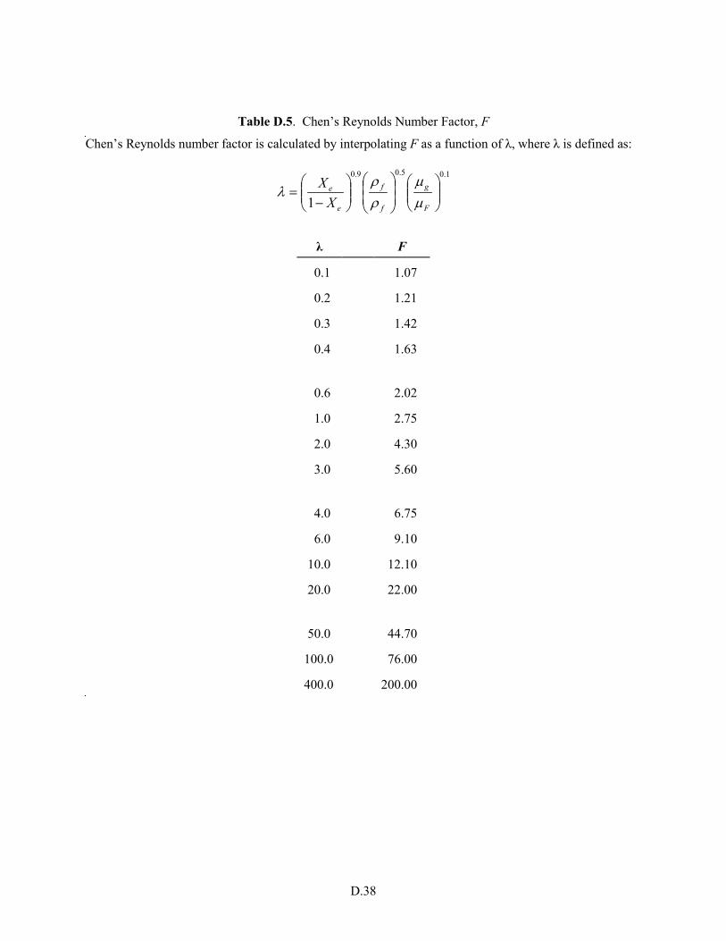
D.38

Table D.5. Chen’s Reynolds Number Factor, F Chen’s Reynolds number factor is calculated by interpolating F as a function of λ, where λ is defined as:

1.05.09.0

1

−

=F

g

f

f

e

e

XX

mm

ρρ

λ

λ F

0.1 1.07

0.2 1.21

0.3 1.42

0.4 1.63

0.6

2.02

1.0 2.75

2.0 4.30

3.0 5.60

4.0

6.75

6.0 9.10

10.0 12.10

20.0 22.00

50.0

44.70

100.0 76.00

400.0 200.00

D.39

Table D.6. The Chen Suppression Factor, S

(Ref)F1.25 S

103 1.000

104 0.893

2 × 104 0.793

3 × 104 0.703

4 × 104 0.629

6 × 104 0.513

105 0.375

2 × 105 0.213 3 × 105 0.142

4 × 105 0.115

6 × 105 0.093

106 0.083

108 0.000

Table D.7. Range of Applicability of Generalized FLECHT Correlation

Variable Applicable Range of Variable

Flooding rate (in./s) 0.4 - 10 Reactor vessel pressure (psia) 15 - 90 Inlet coolant subcooling (°F) 16 - 189 Initial cladding temperature (°F) 300 - 2200 Peak fuel rod power (kW/ft) 0.51 - 1.4 Flow blockage (%) 0 - 75 Equivalent elevation in FLECHT facility (ft) 2 - 10

D.40

Table D.8. Variable and Symbol Definitions in FLECHT Correlation Variables Vin = flooding rate (in./s) Tinit = peak cladding temperature at start of flooding (°F) Q’max = fuel rod power at axial peak at start of flooding (kW/ft) P = reactor vessel pressure (psia) Z = equivalent FLECHT elevation (ft) Tsub = flood water subcooling at inlet (°F) t = time after start of flooding as adjusted for variable flooding rate (s) h = heat transfer coefficient (Btu/hr∙ft2-°F) Qmaxtq = radial power shape factor = 1.0 for a nuclear rod = 1.1 for electrical rod with radially uniform power B = flow blockage (%) (B always set equal to zero) Symbols a**b = ab

Figure D.1. Illustration of FRAPTRAN Forced Convection Heat Transfer Regimes for Full Boiling

Curve

D.41

Figure D.2. Description of Geometry Terms in Coolant Enthalpy Model

Appendix E –

Numerical Solution of the Plenum Energy Equations

E.1

Appendix E: Numerical Solutions of the Plenum Energy Equations

The Crank-Nicolson finite difference form of the six energy equations presented in Section 2.3 is as follows. Plenum Gas:

( )

( ) ( )1111

111

22

2++++

+++

−+−+−+−+

+−−=−

mg

mss

mg

mss

ssssmg

mcli

mg

mcli

clcl

mip

mg

mg

mep

epepm

gm

gggg

TTTThATTTThA

TTTThATT

CVτ

ρ (E.1)

Spring Center Node:

( )111

2++

+

++−+′′′=− m

scm

ssm

scm

ssss

sscsc

msc

msc

sscs TTTTRKAVqTTCV

τρ (E.2)

Spring Surface Node:

( )

( ) ( )1111

111

22)(

2

++++

+++

−+−+−+−+

+

−+−+′′′=−

mss

mg

mss

mg

sssmss

mcli

mss

mcli

concradsss

mss

msc

mss

msc

ss

sscss

msc

msc

ssss

TTTThATTTThhA

TTTTRKAVqTTCV

τρ

(E.3)

Cladding Interior Node:

( )

( ) ( )1111

111

2/22

2++++

+++

−+−∆⋅

+−+−+

−+−+

+′′′=−

mcli

mclc

mcli

mclc

clclmcli

mg

mcli

mg

clcl

mcli

mss

mcli

mss

concssradcclcli

mcli

mcli

clclicli

TTTTrKATTTThA

TTTThAhAVqTTCVτ

ρ (E.4)

Cladding Center Node:

( )

( )11

111

2/2

2/2++

+++

−+−∆⋅

+

−+−∆⋅

+′′′=−

mclc

mclo

mclc

mclo

clcl

mclc

mcli

mcli

mcli

clclclc

mclc

mclc

clclccl

TTTTrKA

TTTTrKAVqTTCV

τρ

(E.5)

Cladding Exterior Node:

11 ++ = mcool

mclo TT (E.6)

E.2

The superscripts m and m+1 represent the values of quantities at the old (m) and new (m+1) time. The steady-state finite difference equations are obtained by setting the left side of Equations (E.1) through (E.5) to zero and by dropping the superscripts m and m+1. Equations (E.1) through (E.5) can be written in the following simplified form by combining constant coefficients and known temperatures (Tj

m). Plenum Gas:

11

11

11

1 ITCTBTA mss

mcli

mg =++ +++ (E.7)

Spring Center Node:

21

21

2 ITDTC msc

mss =+ ++ (E.8)

Spring Surface Node:

31

31

31

31

3 ITDTCTBTA msc

mss

mcli

mg =+++ ++++ (E.9)

Combining Equations (E.8) and (E.9):

31

31

31

3 ITCTBTA mss

mcli

mg =++ +++ (E.10)

where

22

333 C

DDCC −=

22

333 I

DDII −=

Cladding Interior Node:

41

41

41

41

4 ITETCTBTA mclc

mss

mcli

mg =+++ ++++ (E.11)

Cladding Center Node:

51

31

51

5 ITFTETB mclo

mclc

mcli =++ +++ (E.12)

Equations (E.7) through (E.12) represent a set of six equations having six unknowns.

In the above equations, all material properties and heat transfer coefficients (except convection to the coolant) are shown as constants. For the transient case, the temperature-dependent material properties and heat transfer coefficients are evaluated at the average of the temperatures (TBAR) at the start and end times of each time step. For the steady-state calculation, TBAR represents an estimate of the true steady state temperature. Therefore, it is required that the steady state and transient solutions to Equations (E.7) through (E.12) be iterated to convergence on TBAR.

Appendix F –

High-Temperature Oxidation Models in FRAPTRAN-2.0

F.1

Appendix F: High-Temperature Oxidation Models in FRAPTRAN-2.0

F.1 Introduction

FRAPTRAN-2.0 contains both the Cathcart-Pawel (C-P) (Cathcart 1976; Pawel, Cathcart, and Campbell 1979) and Baker-Just (B-J) (Baker and Just 1962) oxidation models. The C-P model calculates oxide thickness, weight gain, and energy generation once cladding average temperature exceeds 1073K (800°C). This model is considered a best-estimate model and is based on oxidation data collected at temperatures greater than 1273K (1000°C); therefore, use of the model at temperatures below 1273K (1000°C) is an extrapolation below the lower bound of the data on which the model was based.

The B-J model calculates oxide thickness and energy generation once cladding average temperature exceeds 1000K (727°C). This model is used in licensing calculations and is based on oxidation data collected at temperatures greater than 1173K (900°C); therefore, use of the model below 1173K (900°C) is an extrapolation below the lower bound of the data on which the model was based.

F.2 Derivation of Cathcart-Pawel and Baker-Just Equations

Cathcart-Pawel

The Cathcart-Pawel model is stated in MATPRO to be

⋅×−

×= −

TKdtdK

314.810502.1exp10126.11 5

6

where K = thickness of oxide layer T = temperature (K) t = time (s)

Rearranging this gives:

dtT

KdK

⋅×−

×= −

314.810502.1exp10126.1

56

Integrating gives

∫∫

⋅×−

×= −2

1

56

2

1 314.810502.1exp10126.1

t

t

K

K

dtT

KdK

2

1

56

2

1

2

314.810502.1exp10126.1

2

t

t

K

K

tT

K

⋅×−

×= −

F.2

tT

KK ∆

⋅×−

×⋅=− −

314.810502.1exp10126.12

562

122

tT

KK ∆

⋅×−

×⋅+= −

314.810502.1exp10126.12

562

122

Baker-Just

The Baker-Just model as stated in the original reference is given by the following equation:

⋅−

×=T

tw987.145500exp103.33 62

where w = mg zirconium reacted per cm² of surface area T = temperature (K) t = time (s)

The Baker-Just model can be converted into a form that predicts oxide layer thickness:

( ) sZrOm

kgZrOm

kgZrkgZrO

mcm

mgZrkgZr

scmmgZr 2

24

22

23

2

22

4

4

26

2

22

26 10883.1

)5680()1(

)74.0()1(

)1()100(

)10()1()(103.33 −×=×××××

so

⋅−

×= −

TtK

987.145500exp10883.1 42

where K is the thickness of oxide layer. For time increment, ∆t = t1-t2

⋅−

∆×+= −

TtKK

987.145500exp10883.1 42

122

or in the form of the Cathcart Pawel equation

⋅−

∆×⋅+= −

TtKK

987.145500exp10415.92 52

122

F.3

F.3 Comparison of Models to Each Other and to Data

The results of simple calculations performed using the equations presented above are presented in Figure F.1. Comparisons of the two models show that they predict nearly the same oxidation growth at 1073K (800°C). For temperatures greater than 1073K, B-J predicts more oxidation growth than C-P, as would be expected based on its reputation and its conservative, licensing-oriented, development. However, for temperatures less than 1073K, which is an extrapolation for both models, C-P predicts more oxidation growth than B-J; this is a reversal of the trend seen for temperatures greater than 1073K.

0.01

0.1

1

10

100

1000

0 200 400 600 800 1000

Time, s

Oxi

de T

hick

ness

, mm

C-P at 600°C C-P at 800°C C-P at 1000°C C-P at 1400°CB-J at 600°C B-J at 800°C B-J at 1000°C B-J at 1400°C

Figure F.1. Comparison of C-P and B-J Models at Temperatures from 600 to 1400°C

Of interest is how the two models compare to oxidation data in the temperature range of 873 to 1273K (600 to 800°C). There is little data available in this temperature range; however, some data (Yoo et al. 2001; Leistikow and Schanz 1984) are compared to the model predictions in Figure F.2. As may be seen from this figure, both models reasonably agree with the data at 600°C, while both models overpredict the data at 800°C.

Reviewing the comparison in Figure F.2, and assuming that FRAPTRAN-2.0 calculations will not exceed more than about 10 to 30 minutes, it was agreed that oxidation calculations by FRAPTRAN-2.0 at temperatures less than 800°C are not needed. Therefore, the historical temperature limits on oxidation of 1073K for C-P and 1000K for B-J in FRAPTRAN-2.0 are retained.

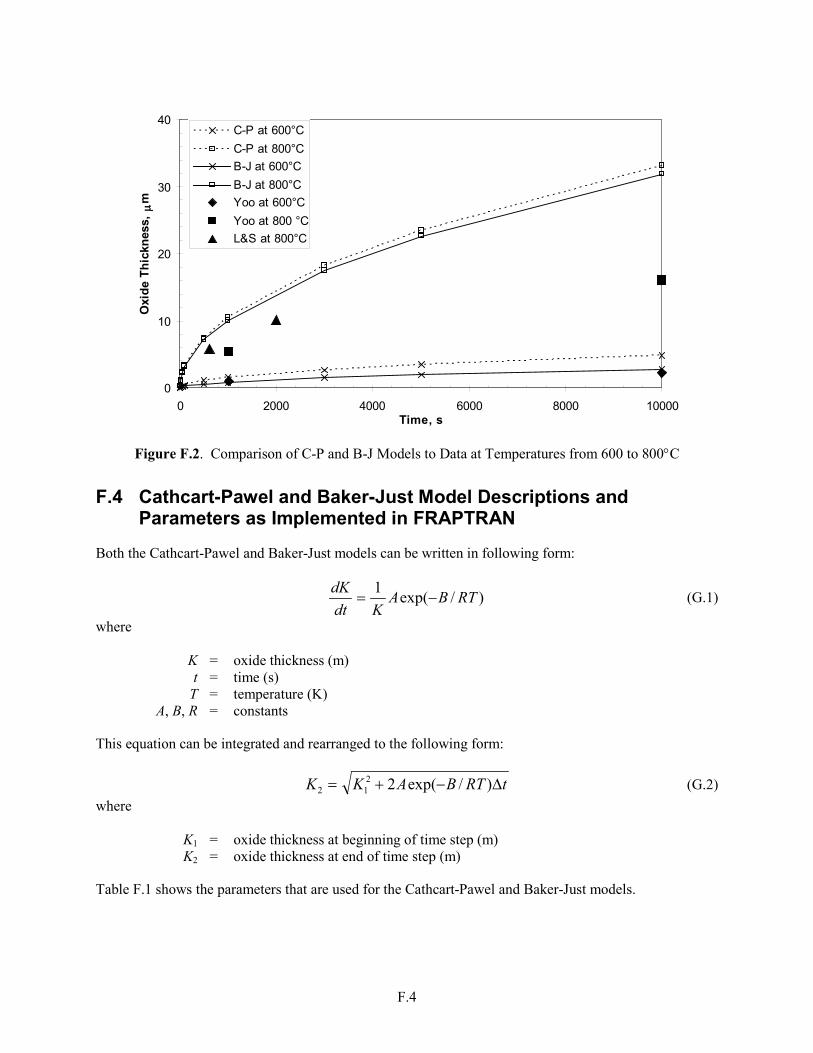
F.4

0

10

20

30

40

0 2000 4000 6000 8000 10000Time, s

Oxi

de T

hick

ness

, mm

C-P at 600°CC-P at 800°CB-J at 600°CB-J at 800°CYoo at 600°CYoo at 800 °CL&S at 800°C

Figure F.2. Comparison of C-P and B-J Models to Data at Temperatures from 600 to 800°C

F.4 Cathcart-Pawel and Baker-Just Model Descriptions and Parameters as Implemented in FRAPTRAN

Both the Cathcart-Pawel and Baker-Just models can be written in following form:

)/exp(1 RTBAKdt

dK−= (G.1)

where K = oxide thickness (m) t = time (s) T = temperature (K) A, B, R = constants

This equation can be integrated and rearranged to the following form:

tRTBAKK ∆−+= )/exp(2212 (G.2)

where K1 = oxide thickness at beginning of time step (m) K2 = oxide thickness at end of time step (m)

Table F.1 shows the parameters that are used for the Cathcart-Pawel and Baker-Just models.

F.5

Table F.1. Constants for Cathcart-Pawel and Baker-Just Models

Constant Cathcart-Pawel Baker-Just A 1.126x10-6 m2/s 9.415x10-5 m2/s B 1.502x105 J/mol 4.55x104 cal/mol R 8.314 J/mol-K 1.987 cal/mol-K

The following shows how oxidation is calculated in FRAPTRAN-2.0 cobild (Cathcart Pawel OD) c az3 is the time increment for the integration. c az8 = av. temp. during increment y6 = 2.0d0 * (1.12569d-02) * exp(-3.58908d04/(1.987d0 * az8)) y8 = sqrt(y8**2 + y6 * az3) Note: 1.502x105 J/mol = 3.5874x104 cal/mol chitox (Cathcart Pawel ID) c x1 = input zro2 thickness at start of a time step (m) c x2 = output zro2 thickness at the end of a time step (m) x2 = sqrt((x1)**2 + 2.0d0 * (1.12569d-06) + * exp(-3.58908d04/(1.987d0 * tave))*dt) metwtb (Baker Just OD and ID) dm2 = sqrt(dm1**2 + 1.883d-4 * exp(-45500.0d0/1.987/tave) & * TimeIncrement) Note: Factor of 2 from Equation 2 is included in constant A

Table F.2 shows how the high temperature oxidation outputs, OD and ID oxide thickness, OD and ID oxygen uptake, ECR, and metal water reaction energy are calculated in FRAPTRAN-2.0.

Table F.2. High-Temperature Oxidation Outputs from FRAPTRAN-2.0

Parameter FRAPTRAN Variable Cathcart-Pawel Baker-Just OD oxide thickness

EOSOxideThick (in.)

comput calls cobild heat calls metwtb

ID oxide thickness OxiThk2 (in.)

heat calls chitox heat calls metwtb

OD oxygen uptake OxygenUptake (kg/m²)

comput calls cobild and uses parameters recommended by C-P

store6 calculates from EOSOxideThick

ID oxygen uptake OxUptakeID2 (kg/m²)

heat calls chitox and uses parameters recommended by C-P

store6 calculates from OxiThk2

Total ECR ECR (fraction)

store6 calculates from OxygenUptake and OxUptakeID2

store6 calculates from OxygenUptake and OxUptakeID2

Metal water reaction energy

WatrMetlEnrgy (kW/ft)

comput calls cobild for OD power. heat calls chitox for ID power and adds it to OD power

heat calls metwtb for OD power. heat calls metwtb for ID power and adds it to OD power

F.6

F.5 References

Baker L Jr. and LC Just. 1962. Studies of Metal-Water Reactions at High Temperatures III. Experimental and Theoretical Studies of the Zirconium-Water Reaction. ANL-6548, Argonne National Laboratory, Argonne, IL.

Cathcart J.V. 1976. Quarterly Progress Report on the Zirconium Metal-Water Oxidation Kinetics Program Sponsored by the NRC Division of Reactor Safety Research for April-June 1978. ORNL/NUREG/TM-41, Oak Ridge National Laboratory, Oak Ridge, TN.

Leistikow S and G Schanz. 1984. “High Temperature Oxidation of Zircaloy-4 Cladding Tubes in Steam (600-1600°C).” In 9th International Congress on Metallic Corrosion, Toronto, Canada, 3-7 June, pg. 282-287.

Pawel RE, JV Cathcart, and JJ Campbell. 1979. “The Oxidation of Zircaloy-4 at 900 and 1100°C in High Pressure Steam.” J. Nuclear Materials 82:129-139.

Yoo H-I, et al. 2001. “A Working Hypothesis on Oxidation Kinetics of Zircaloy.” J. Nuclear Materials 299:235-241.

fraptran-2.0: a computer code for the transient … code for the transient analysis of oxide fuel...

Documents