Fraternity Membership and Binge Drinking

Jeff DeSimone*

University of South Florida and NBER

26 December 2006

Abstract

This paper examines the relationship that social fraternity and sorority membership has

with binge drinking incidence and frequency among 18–24 year old full-time four-year college

students who participated in the 1995 National College Health Risk Behavior Survey. To net out

unobserved heterogeneity, several measures of situational and total alcohol use are entered into

the regressions as explanatory variables. Fraternity membership coefficients are substantially

reduced in size, but remain large and highly significant, suggesting a causal effect on binge

drinking. Otherwise, the estimates identify idiosyncratic selection into fraternities and binge

drinking across students with similar overall drinking profiles. Particularly notable is that

behavior by underage students appears to drive the relationship.

* Department of Economics, University of South Florida, 4202 E. Fowler Ave., BSN 3403, Tampa, FL 33620-5500; Phone: (813) 974-6514; E-mail: jdesimon@coba.usf.edu. I thank Joseph Newhouse and two anonymous referees for helpful suggestions.

1. Introduction

Social fraternities and sororities play a prominent role in the lives of U.S. college

students. Eighteen percent of 18–24 year old full-time, four year college students in the 1995

National College Health Risk Behavior Survey (NCHRBS) were fraternity members, as were 12

percent of 17–25 year old four year college students in the 2001 Harvard College Alcohol Study

(CAS).1 Collegiate fraternities were founded largely to advocate community service, leadership

and learning. While many still fill these roles, fraternities now exist primarily as a focal point for

developing friendships among students interested in similar social activities.2

The main activity with which fraternities are associated is alcohol use. Fraternities often

connote a culture of drunkenness, as famously portrayed in the movie Animal House. Anecdotal

evidence of problem drinking at fraternity events abounds. Data confirm that fraternity members

drink more intensively than do non-members. In the NCHRBS, past month binge drinking,

defined as consuming at least five alcoholic beverages within a few hours, was reported by 69

percent of fraternity members as compared with 42 percent of non-members.3 Analyses of data

from the CAS (Chaloupka and Wechsler, 1996) and the Core Alcohol and Drug Survey (Alva,

1998; Cashin et al., 1998) have similarly documented that fraternity members drink more

frequently and heavily than do their non-member peers.

It is tempting to assume that fraternity membership is the reason that fraternity members

drink more excessively than do non-members. But does fraternity membership truly cause binge

drinking? Specifically, would the incidence or frequency of binge drinking among students who 1 Throughout the paper, the term “fraternity” applies in a gender-nonspecific way to both fraternities and sororities. 2 Analogous organizations are rare outside the U.S. and Canada, but do exist in countries such as the Netherlands, Belgium, Germany and the Philippines (see http://en.wikipedia.org/wiki/Fraternities_and_sororities). 3 A weakness of binge drinking as a proxy for drunkenness is that those who are heavier or otherwise have a greater tolerance to alcohol require more drinks to become intoxicated. The National Institute of Alcoholism and Alcohol Abuse and Centers for Disease Control have adopted a four-drink threshold to define binge drinking for women, who tend to be lighter and binge drink less frequently than men (see www.hsph.harvard.edu/cas/), but the NCHRBS used the five drink threshold for all respondents.

1

join fraternities decline in the absence of fraternities? That is the question this study addresses.

College student binge drinking is a concern because it is associated with many behaviors

that are harmful, particularly to others. These include drunken driving (Hingson et al., 2003b),

violence (Wechsler et al., 1995), vandalism and related disturbances (Wechsler et al., 2002),

sexual activity that is forced (Mohler-Kuo et al., 2004) or risky (Hingson et al., 2003a), and

reduced academic performance (Kremer and Levy, 2003). Efforts that most effectively limit

external binge drinking effects depend in part on whether fraternities increase binge drinking.

Furthermore, any direct effect of fraternity membership on binge drinking underestimates

the corresponding total effect, which also includes the impact on drinking by non-members. For

instance, Chaloupka and Wechsler (1996) find that having a fraternity on campus increases the

likelihood of binge drinking regardless of membership status, while Glindemann and Geller

(2003) estimate that intoxication levels at fraternity parties exceed those at other parties.

Moreover, fraternity-induced binge drinking might lead to binge drinking among roommates or

other peers (e.g. Kremer and Levy, 2003; Lundborg, 2006).

Students who join fraternities presumably perceive that membership will facilitate desired

binge drinking by matching them with students who share these preferences. For example,

Sacerdote (2001) found that high school drinkers in the Dartmouth senior classes of 1997 and

1998 were more likely to join a fraternity than were other classmates. Baer et al. (1995), Schall

et al. (1992) and Wechsler et al. (1996) obtain similar evidence and report that among students

who drank in high school, those who joined fraternities were more likely to have binge drank.

If self-selection of binge drinkers into fraternities is responsible for the correlation

between drinking and fraternity membership, members would binge drink even if fraternities did

not exist, and binge drinking therefore cannot be attributed to membership. In contrast, Borsari

2

and Carey (1999) outline three ways in which fraternity membership might increase binge

drinking. One is by applying social pressure to drink in order to gain acceptance among fellow

members. Another is by elevating perceptions of peer drinking norms, which college students

already tend to overestimate. The third is by providing an environment that makes alcohol

readily available and is insulated from students less tolerant of binge drinking. Consistent with

this, Lo and Globetti (1995) find that students who do not previously binge drink are three times

more likely to start doing so if they join a fraternity. Also, Sher et al. (2001) estimate that

fraternity members drank more heavily than non-members during college, even controlling for

previous alcohol use, but that this discrepancy disappeared within three years after college.

This study infers the effect of fraternity membership on binge drinking using a proxy

variable approach. It specifically includes various potentially endogenous factors as covariates

to control for unmeasured binge drinking determinants that might be correlated with fraternity

membership. Importantly, the main proxies are measures of current period alcohol use defined

more broadly than binge drinking. The fraternity effect is ultimately identified using differences

between members and non-members who drink in identical frequencies and situations.

As there is no way to know whether proxy variables completely eliminate spurious

regression correlations, it is overly ambitious to claim that the study estimates the causal effect of

fraternity membership on binge drinking. Yet, the alcohol use measures do explicitly control for

the exact type of unobserved heterogeneity that is most likely to contaminate the relationship of

interest. Moreover, this approach attributes a sizable portion of the observed variation in binge

drinking to related behaviors that in fact might be directly influenced by fraternity membership.

The analysis hence yields an estimated fraternity effect that is prospectively conservative.

If nothing more, it isolates a non-causal component of the relationship that fraternity membership

3

has with binge drinking, and outlines the selection mechanisms that must prevail to invalidate the

interpretation of the remaining correlation as causal. Namely, for the causality argument to fail,

fraternity membership must not influence non-binge drinking, and students must opt to join

fraternities because they binge drink more often than non-members who otherwise consume

alcohol with similar frequency, in analogous situations and over the same time period.

2. Data and Empirical Strategy

In estimating the binge drinking effect of fraternity membership, the main econometric

issue is the presence of unobserved factors that simultaneously determine membership and

binging. If binge drinking preferences are a reason that students join fraternities, members

would binge drink more than non-members even in the absence of fraternities. This omitted

variable problem must be addressed so that the fraternity membership regression coefficient

reflects only binge drinking that would not have occurred if fraternities did not exist. In

attributing endogeneity solely to omitted variables, I dismiss the possibility of reverse causation.

Student rarely leave fraternities, and holding constant unobserved confounding factors, it seems

unlikely that an exogenous increase in binge drinking would induce a student to join a fraternity.

The identification strategy includes observable factors that approximate omitted binge

drinking preferences likely correlated with fraternity membership. A distinctive aspect is the use

of several alcohol consumption measures to reflect these preferences, specifically measures of

drinking frequency, duration and the incidence of drinking in several circumstances that are

particularly risky. Any persistent self-selection would have to involve binge drinking differences

between members and non-members who have similar patterns of non-binge alcohol use.

Moreover, if non-binge drinking is also influenced by fraternity membership, this approach could

4

yield conservative estimated fraternity effects.

These alcohol covariates supplement a baseline model that controls for many standard

personal characteristics, and in some models are accompanied by proxies for additional omitted

factors. The vector of controls thus includes a fraternity membership indicator (F), variables

arguably exogenous with respect to unobserved binge drinking determinants (X), alcohol use

covariates representing unobservables that influence fraternity membership and binge drinking

(A), and additional heterogeneity controls (U). A regression equation incorporating this is

B = α0 + α1F + Xα2 + Aα3 + Uα4 + ε, (1)

where B represents binge drinking, ε ~ N(0, σ2) includes unobserved determinants of binge

drinking, and the α are the regression parameters.

Variants of equation (1) are estimated using data from the National College Health Risk

Behavior Survey (NCHRBS), developed by the Centers for Disease Control (CDC) and

administered during the first half of 1995.4 As described in CDC (1997), the NCHRBS was

designed to monitor college student health-risk behaviors. Two-stage cluster sampling produced

a nationally representative group of undergraduates aged 18 and over. From 16 strata with

varying percentages of black and Hispanic students, the first stage selected 148 institutions, half

two-year and half four-year, with probability proportional to undergraduate enrollment. The

second stage randomly sampled undergraduates in the 136 institutions that chose to participate,

targeting 72 and 56 students from each two- and four-year school, respectively. The

questionnaire was mailed to 7,442 students for self-administration and completed by 4,814.

The analysis sample is restricted to 18–24 year old, full-time undergraduates from four-

year schools. In 1995, 57 percent of the 12 million U.S. college students were ages 18–24, and

4 Specific interview dates are not reported.

5

few students who are older, part-time or at two-year schools are fraternity members.5 Sensitivity

analyses later verify that these exclusion criteria do not drive the estimation results.

The two dependent variables in the regressions are constructed from information on the

number of days in the past 30 on which the respondent binge drank. One is an indicator of any

binge drinking, for which probit models are estimated. Tables report average marginal effects.

The other dependent variable is binge drinking days. Because the survey reports only the

categorical choice between 0, 1, 2, 3–5, 6–9, 10–19, and 20 or more, binge days is analyzed

using an interval regression model. This handles the lower bound of zero and upper bound of 20

identically to a Tobit model. It further recognizes that while values of 1 and 2 represent exact

numbers of days, all that is known about the remaining three categories are the lowest and

highest number of days that corresponding values could represent.

Rewriting equation (1) as B = Zα + ε, the likelihood function for the interval model is

∑∑

∑∑

∑ ∑∑

∈∈

∈∈

= ==

⎥⎦

⎤⎢⎣

⎡⎟⎠⎞

⎜⎝⎛ −

Φ−+⎥⎦

⎤⎢⎣

⎡⎟⎠⎞

⎜⎝⎛ −

Φ−⎟⎠⎞

⎜⎝⎛ −

Φ+

⎥⎦

⎤⎢⎣

⎡⎟⎠⎞

⎜⎝⎛ −

Φ−⎟⎠⎞

⎜⎝⎛ −

Φ+⎥⎦

⎤⎢⎣

⎡⎟⎠⎞

⎜⎝⎛ −

Φ−⎟⎠⎞

⎜⎝⎛ −

Φ+

⎥⎥⎦

⎤

⎢⎢⎣

⎡+⎟

⎠⎞

⎜⎝⎛ −

−⎥⎥⎦

⎤

⎢⎢⎣

⎡+⎟

⎠⎞

⎜⎝⎛ −

−⎟⎠⎞

⎜⎝⎛−Φ=

]30,20[]19,10[

]9,6[]5,3[

0 2

22

1

22

201log1019log

69log35log

2log2212log1

21log

BB

BB

B BBL

σσσ

σσσσ

πσσ

πσσσ

ZαZαZα

ZαZαZαZα

ZαZαZα

, (2)

where Ф() is the cumulative standard normal distribution.6 The tables report marginal effects on

the observed B, calculated by multiplying the coefficients by ⎟⎠⎞

⎜⎝⎛−Φ−

σZα1 , i.e. the probability

that B > 0. This adjusts the coefficient downward in magnitude because the actual coefficients

represent marginal effects on the underlying B*, which can be negative, but the lower bound of

5 Also, one quarter of U.S. residents age 18–24 were college students. 6 Because the assumption of a normally distributed regression error is critical to both the probit and interval models, OLS results for both dependent variables are later presented as a robustness check.

6

zero is a true corner solution.7 Reported marginal effects again are averages across respondents.

The key explanatory variable, F, indicates whether the student is a member of a social

fraternity. This does not take into account fraternity house residence, which is later shown to be

irrelevant. Only 22 percent (57 of 259) of sample fraternity members live in a fraternity house.

The vector X of exogenous drinking determinants includes indicators for females, ages

18–24 (age 21 omitted), the freshman, sophomore and junior classes (seniors omitted), non-

Hispanic blacks, Hispanics, Asians and other non-white, non-Hispanics (non-Hispanic whites

omitted), married and separated, divorced or widowed (never married omitted), each parent not

finishing high school, graduating from high school, attending college and having unknown

education (graduating from college omitted), and each institution sampled except one. The

school fixed effects, though not strictly exogenous, are important to include as controls for

student selection into schools based on drinking prevalence and fraternity availability.

The vector A consists of the five alcohol measures alluded to above, which are intended

to reflect preferences that might influence fraternity membership and binge drinking. The

number of days alcohol was consumed, and number of times it was used before driving and in

combination with illegal drugs, each represent the past 30 days and are collapsed from

categorical responses by assigning midpoints and top-codes. Choices were zero, 1–2, 3–5, 6–9,

10–19, 20–29, and 30 for drinking days, zero, 1, 2–3, 4–5, and 6 or more for drunk driving, and

0, 1–2, 3–9, 10–19, 20–39, and 40 or more for use with drugs. Top-codes of 6.4 for drunk

driving (three percent of the sample) and 40 for use with drugs (0.1 percent) are imputed by

assuming an underlying normal distribution and rounding to the nearest tenth.

The other two alcohol use proxies are an indicator of whether alcohol or drugs were used

7 The constraint B* ≤ 30 need not be imposed because it is not binding: only seven respondents report 20 or more binge days, and the predicted B* for these (and all other) respondents is always less than 20.

7

before the most recent sexual encounter, and the number of years since alcohol was first

consumed. The latter is formed by subtracting from current age the reported age at which the

respondent first drank more than a few sips of alcohol, choices for which were never, 12 or

younger, 13–14, 15–16, 17–18, 19–20, and 21–24. The age of first drink was set equal to current

age for those who had never drank (which converts to zero years of drinking), 19 year olds

reporting 19–20, and 21 year olds reporting 21–24; 12 for those reporting the youngest category

(12 percent of the sample); interval midpoints for all reporting 13–14, 15–16 and 17–18, 20 year

olds reporting 19–20 and 24 year olds reporting 21–24; 21.5 for 22 year olds reporting 21–24;

and 22 for 23 year olds reporting 21–24.

Consumption frequency and duration are meant to broadly reflect tastes for alcohol. The

drinking before sex and concurrently with illegal drugs variables are motivated by Cashin et al.

(1998), who find that fraternity members are more likely to view drinking as a vehicle for sexual

opportunity and experience negative consequences from alcohol and other drugs. Meanwhile,

fraternity members might be more disposed to driving drunk if fraternities are non-residential

and host events at which alcohol is available. With these covariates included, the effect of

fraternity membership is identified by comparing members and non-members who have

consumed alcohol for the same length of time and roughly the same number of days in the past

month, drove and used an illegal drug while drinking about the same number of times, and had

the same drinking status the last time they had sex. Remaining self-selection into fraternities

picked up by the fraternity coefficient must occur on the basis of idiosyncratic tastes for binging.

Measurement error associated with constructing numerical variables from the categorical

information works against the identification strategy. Even if this error is random, the estimated

correlation between these variables and binge drinking will be smaller than if alcohol use was

8

measured precisely. This is exacerbated if the measurement error is correlated with fraternity

membership, which would thereby show lower correlation with the alcohol use controls.

Offsetting this is the possibility that the alcohol variables represent drinking behavior that in fact

responds to fraternity membership, which would deflate the estimated binge drinking effect.

Finally, the vector U includes several other covariates that potentially absorb some of the

unobserved heterogeneity between fraternity membership and binge drinking. To separate the

effects of physical environment and membership, a set of indicators reflect whether respondents

live in a residence hall, fraternity or sorority house, other institutional housing, off-campus

residence, or parent or guardian’s home, with “other” as the omitted category. Because paid

employment might have both substitution and income effects on membership and drinking, a

variable representing weekly hours of paid work is constructed from choices of zero, 1–9, 10–19,

20–29, 30–39, 40, and more than 40, using interval midpoints and a top code of 45. The number

of sports teams on which the respondent played (intra- or extramural), with a top-code of 3.3

assigned for the “3 or more” category, and height each might proxy for popularity (Persico et al.,

2004). Bodyweight helps determine the amount of alcohol necessary to cause inebriation.

The U vector has three additional elements. An indicator for always wearing a seat belt

when riding in a car (as opposed to most of the time, sometimes, rarely or never) is included as a

measure of risk aversion (Hersch and Pickton, 1995). The number of cigarettes smoked in the

past 30 days, formed by multiplying days smoked and the number smoked per day, proxies for

time preference (Evans and Montgomery, 1994; Fersterer and Winter-Ebmer, 2003). The days

smoked variable parallels that for alcohol, while midpoints and a top-code of 21 are assigned for

cigarettes per day categories of zero, less than one, one, 2–5, 6–10, 11–20, and more than 20.

Finally, the number of past 30 days uses of marijuana accounts for a potential interrelationship

9

between alcohol and marijuana, which Williams et al. (2004) report to be complementary for

college students. This is recoded, using a top-code of 41, from a variable with the same

categories as the alcohol and drug combination variable.

The analysis sample size is 1,401, from 66 different schools representing between four to

48 students. As table 1 documents, this includes only those for whom all variables are observed.

To verify robustness, models adding respondents for whom the only missing information

pertains to a U variable are also estimated. All regressions use NCHRBS sampling weights.

Because these do not incorporate my idiosyncratic exclusion criteria, I later show estimates from

an unweighted specification. Standard errors are robust to arbitrary forms of heteroskedasticity.8

Weighted sample means are provided in table 2. Column 1 shows unconditional means,

while columns 2 and 3, respectively, show means for fraternity members, who comprise 18

percent of the sample, and non-members. Nearly half of respondents binge drank at least once in

the past 30 days. The binge days mean of 2.5 thus implies that binge drinkers did so on five of

the past 30 days on average. As expected, binge drinking is more prevalent and frequent among

fraternity members. Fraternity binge drinkers did so an average of 6.7 days, compared to 4.8

days for non-member binge drinkers. Members are more likely than non-members to be male, in

the middle of the age distribution, juniors and seniors, white, and unmarried, and to have mothers

who attended college and fathers who graduated from college. Overall and situational alcohol

use is also more common among members. Fraternity housing appears to crowd out off campus

housing rather than dormitories. Members also work fewer hours in paid jobs, are taller and

heavier, play on more sports teams, and use cigarettes and marijuana more often.

8 The precise notation for equation (2), therefore, would have each term multiplied by a weight variable, and add a subscript to σ2 signifying that it can vary across observations.

10

3. Results

a. Baseline estimates

Table 3 shows results for baseline models that do not control for heterogeneity proxies.

Columns 1 and 4 indicate large and highly significant unconditional relationships between

fraternity membership and binge drinking, with implied semi-elasticities of 0.57 for any drinking

and 0.84 for drinking days at the dependent variable means. Adding student characteristics in

columns 2 and 5 reduces the fraternity coefficient sizes, but by only 18–19 percent. Rather than

absorbing some of the self-selection of binge drinkers into fraternities, entering school fixed

effects in columns 3 and 6 slightly increases the fraternity coefficients. Members are more likely

to binge drink by 23 percentage points (i.e. 48 percent), and binge drink on 1.7 additional days

(i.e. 68 percent). These seem too large to reflect causal effects, warranting the subsequent

insertion of the previously described controls for unobserved confounders.

Columns 2 and 3 also show the coefficients of the exogenous variables besides the school

indicators. Binge drinking is more common among males and whites, as holds the conventional

wisdom (e.g. http://kidshealth.org/college/drug_alcohol/getting_help/binge_drinking.html), as

well as the unmarried, but is not significantly related to age, grade, or parental education.9

b. Adding alcohol use covariates

Table 4 presents results for models that include alcohol use covariates to account for self-

selection of students into fraternities based on drinking preferences. The dependent variable is

the binge drinking indicator in columns 1 and 2 and binge drinking days in columns 3 and 4.

The starting point is the specification in columns 3 and 6 of table 3, i.e. with school fixed effects.

Columns 1 and 3 add days of drinking in the past 30 days. These models imply that 9 Age and grade are highly correlated, but all indicators for one remain insignificant even when the other is omitted.

11

fraternity membership causes binge drinking solely by increasing its likelihood on days when

alcohol would have been consumed regardless. This assumption seems particularly strong;

indeed, the total drinking days variable has the largest impact by far among the alcohol use

measures. Its insertion reduces the fraternity coefficient by 60 percent for any binging and 72

percent for binge days. The associated pseudo R-squared statistic, i.e. one minus the ratio of the

model and constant-only log likelihoods, rises by 0.31 for binge drinking propensity and 0.25 for

frequency. Six more days of alcohol use, roughly the standard deviation, predicts binge drinking

increases of 31 percentage points in probability and nearly two days. Importantly, however, the

fraternity effect remains highly significant, in part because the smaller regression standard errors

(i.e. larger pseudo R-squareds) translate to sizable coefficient standard error reductions.10

Estimates for models that include all five alcohol covariates appear in columns 2 and 4.

The total drinking days coefficient remains large, and the only variable to enter insignificantly is

using alcohol with drugs in column 2. But the additional alcohol measures increase the pseudo

R-squareds only slightly, while the fraternity coefficient actually grows in column 2 and shrinks

minimally in column 4. Fraternity membership now increases the likelihood of binge drinking

by 10 percentage points and binge days by about one-half. The associated semi-elasticities of

around 0.2 are economically meaningful, but much more plausible as potential causal effects.

Do these coefficients indeed represent causal impacts of fraternity membership? It is

easily imaginable that fraternity membership influences total drinking days as well as the other

alcohol covariates besides years since first drink. If so, including them might yield conservative,

10 Using non-binge drinking days, i.e. total drinking days less binge drinking days, in place of total drinking days results in much less conservative fraternity coefficients of .200 (6.36) for any binge drinking and 1.57 (6.54) for binge drinking days, where parentheses contain t statistics. By definition, the most frequent binge drinkers rarely drink without binging, which induces a negative correlation between binge and non-binge days. Indeed, when the remaining heterogeneity controls in tables 4 and 5 are inserted, the effect of non-binge days becomes marginally insignificant for any binge drinking and negative (albeit extremely small) for binge days.

12

rather than overstated, causal effect estimates. Even if not, for the fraternity coefficient to reflect

only spurious correlation, remaining selection would have to occur on binge drinking but not be

related to drinking experience, overall drinking frequency and three specific drinking behaviors

that are highly correlated with binge drinking. This scenario seems somewhat convoluted.

Yet, the pseudo R-squareds reveal that the regressions leave unexplained a substantial

portion of the variation in binge drinking. Combined with the reality that it is impossible to be

certain that all unobserved heterogeneity has been eliminated, the case for causality is not

unassailable. Still, the possible influence of further omitted factors can be investigated.

c. Adding other unobserved heterogeneity proxies

To do so, table 5 adds other self-selection controls. Starting with the models in columns

2 and 4 of table 4, which contain all the alcohol use covariates, columns 1 and 3 of table 5

append the three new heterogeneity proxies that are significantly related to binge drinking. Most

notably, students with greater sports involvement are heavier drinkers, with playing on an

additional team raising binge likelihood by 10 percent and days by eight percent. The coefficient

of not wearing a seat belt is slightly smaller in the likelihood equation and slightly larger in the

days equation. This suggests that students who are more popular and risk-tolerant have greater

involvement in binge drinking and fraternities, the latter given the accompanying decline in

fraternity coefficient magnitudes.

In several respects, though, the table 5 results continue to support a causal interpretation

of the fraternity effect. First, the relationship between cigarette smoking and binge drinking is

small and, in the case of any binge drinking, insignificant. Smoking an additional 100 cigarettes,

which is 250 percent of the sample mean, is associated with binge drinking increases of only 1

13

percentage point in likelihood and 0.09 days. The implication is that time preference has little

bearing on binge drinking behavior conditional on the included controls, and therefore does not

induce much spurious correlation between binge drinking and fraternity membership. Second,

the remaining heterogeneity proxies in columns 2 and 4 are highly insignificant both individually

and, as implied by the minimal pseudo R-squared increases, as a group. Third, the change in

fraternity coefficients from columns 1 to 2 and columns 3 to 4 is negligible for any binge

drinking and positive for binge days. Fourth, the net fraternity effect reduction from columns 2

and 4 in table 4 to the same columns in table 5 is only 8–9 percent. Fifth, much like total

drinking days, the main confounder in table 5, playing on sports teams, could in fact be a

mechanism by which fraternity membership influences binge drinking. In particular, fraternities

often field intramural sports teams and might treat competitions as binge drinking occasions.11

Pseudo R-squared statistics that are considerably less than one imply remaining scope for

other sources of spurious correlation between fraternity membership and binge drinking. To

further investigate, I obtain estimates for samples stratified on the covariates listed in tables 4

and 5. In many cases, I form two samples consisting of respondents with low and high values of

the covariate. If selection is important, coefficients in both sub-samples should be relatively

small, because some of the relationship between fraternities and binge drinking is explained by

changes from below average to above average rates of both membership and binging when

moving from one group to the other. Results, available from the author, suggest that self-

selection does not explain the fraternity coefficients. Effects remain significant and sizable for

frequent and infrequent drinkers, more and less experienced drinkers, and students who did not

drink and drive or combine alcohol with drugs or sex, and are quite large for students who drove,

11 No information is available regarding whether the teams represented by the sports variable are intercollegiate or intramural.

14

used drugs or had sex while drinking. Fraternity effects are also considerable for students who

smoke cigarettes or marijuana, are tall or heavy, live on campus, or work, yet retain practical and

statistical significance for the residually defined groups. Finally, although effects are smaller for

athletes and non-athletes alike, fraternity coefficients are still significant for both groups.

d. Method and sample permutations

Table 6 explores whether fraternity effects are sensitive to various method and sample

permutations. Columns 1 and 3 include only student characteristics and school indicators and

are thus comparable to columns 3 and 6 of table 3. Columns 2 and 4 also control for alcohol

covariates, sports participation, seat belt use and cigarette smoking, analogous to columns 1 and

3 of table 5. Each row represents a different method (A. and B.) or sample (C. through J.).

Estimated fraternity membership effects are robust to a wide array of changes, remaining

economically large and statistically significant. The widest deviations occur when the estimation

method is modified in the top two rows. Coefficients are generally smallest in the unweighted

models (row A.), but largest in the OLS models (row B.). The probit and interval models thus

yield conservative estimates relative to OLS, except in column 2 where the opposite is true. In

the rest of the table, the estimates vary little in response to altering the sample by adding students

who are missing values of unimportant variables, older, part-time, or at two-year schools (rows

C.– F.), or omitting students who are behind grade level, currently or previously married, or

attending schools with no or few sample fraternity members (rows G.–J.)

e. Stratifying on exogenous factors

Table 7 contains results of five separate exercises in which two subsamples are formed

15

based on values of a table 3 explanatory variable, with columns 1–4 mimicking table 6. Panels

A. and B. are instructive about how insufficiently accounting for selection can yield misleading

inferences. Columns 1 and 3 suggest that fraternity effects are much stronger for males and

whites, which would be a reason for higher binge drinking rates among these groups. Entering

the heterogeneity proxies in columns 2 and 4, however, considerably reduces these differences.

In A., the remaining discrepancy between male and female coefficients is smaller than their

standard errors. This indicates that targeting alcohol policies at fraternities rather than sororities

as well might be unwise. The gap between whites and nonwhites in B. is wider, and fraternities

no longer increase nonwhite binge days. Yet, the effect on any binging remains significant for

nonwhites, and the binge days effect for whites is lowered by nearly 80 percent.

Panel C. implies that fraternity membership might account for the conventional wisdom

that binge drinking is especially prevalent among underclassmen, given that table 3 showed no

direct association with class standing once membership is held constant. This is especially true

in columns 2 and 4, as selection effects are larger for juniors and seniors than for freshmen and

sophomores. Although NCHRBS data are insufficient to test this claim, one contributing factor

might be that fraternity rushing often occurs by sophomore year and involves binge drinking.

Panel D. divides the sample based on whether respondents are at least age 21 and hence

old enough to drink legally. This reveals a noteworthy result: fraternity coefficients are above

the baseline values for the underage, but are effectively zero for those of legal age. Providing

access to alcohol for those without legal means to obtain it thus appears to be an important

avenue through which fraternities increase binge drinking. This might help to explain the

absence of age effects in table 3. An implication is that directing underage drinking crackdowns

towards fraternities, and particularly their members, could be an efficient way to reduce

16

underage binge drinking as well as fraternity-related campus alcohol problems.

The estimates in C. and D. are also consistent with the other two reasons that Borsari and

Carey (1999) give to explain the means by which fraternities increase binge drinking. Social

pressure to binge drink could be more intense for new pledges trying to fit in than for veteran

members. Similarly, observed drinking at fraternity events might inflate peer drinking norms

less as students acquire experience in various campus social settings and thereby have

opportunities to gain a more representative perspective about drinking among their classmates.

In contrast, panel E. indicates that parental education is inconsequential for fraternity

effects on binge drinking. Parental college and fraternity experience therefore appears irrelevant.

4. Conclusion

Using data on 18–24 year old full-time four-year college students who participated in the

1995 NCHRBS, this study examined the relationship between binge drinking and membership in

social fraternities and sororities. The primary contribution was to enter various measures of

situational and overall alcohol use as explanatory variables in regressions of binge drinking on

fraternity membership. This addresses the specific type of unobserved heterogeneity expected to

inflate the estimated fraternity effect: students who like to drink heavily are the ones who join

fraternities. Including these alcohol use covariates substantially reduced fraternity membership

coefficients. But the continued significance of these coefficients, both statistically and

economically, supports the hypothesis that fraternity membership increases binge drinking.

The main caveat is that the alcohol use and other unobserved heterogeneity proxies might

not fully control for endogenous selection into fraternities. Thus it is impossible to be certain

that the fraternity coefficient represents a causal effect. At a minimum, however, a very

17

idiosyncratic selection mechanism must prevail for these results to not imply some causal effect.

In particular, fraternity members must binge drink more than non-members, yet consume alcohol

in similar frequencies and situations and over similar lengths of time. Moreover, an instrumental

variables method, which is infeasible with these data, would suffer from analogous uncertainties

regarding the correlation between the instruments and unobservable binge drinking determinants.

Also, the analysis does not attempt to correct for measurement error. While this could bias

estimates up if binging is over-reported by fraternity members or under-reported by non-

members, random measurement error would impart downward bias.

Combined with evidence on interventions intended to reduce binge drinking by college

students, the positive impact of fraternity membership on binge drinking suggests specific

strategies that could be targeted towards fraternity members. DeJong et al. (2006) find that

randomly assigned social norms marketing campaigns reduced perceived and actual drinking,

while Trockel et al. (2003) report that perceived drinking was related to actual drinking among

members of two large national fraternities surveyed on a number of campuses. This implies that

efforts to lower peer drinking norms within fraternity chapters might be useful. Also, Barnett et

al. (2006) indicate that mandating attendance in an alcohol education session following alcohol-

related medical treatment or disciplinary infractions can motivate students to change their

drinking behavior, particularly if they feel responsible for the corresponding incident. The

earlier-outlined theories for causal fraternity effects on binging suggest attempting analogous

fraternity-wide education efforts after adverse events involving binge drinking by members or at

fraternity-sponsored parties. Consistent with my findings for the underage, Larimer et al. (2001)

shows that first-year fraternity members randomly assigned an educational intervention of one-

hour individual and housewide discussions reported significant reductions in alcohol use one

18

year later, regardless of whether sessions were conducted by peers or professional staff.

Sacerdote (2001) found that peer effects among room- and dorm-mates are a major

determinant of whether Dartmouth students joined a fraternity. Along with my results, this

implies that fraternity membership is one way through which peers influence binge drinking.

Assigning freshmen who appear likely to join fraternities to the same rooms and dorms might

limit fraternity membership and thus binge drinking.

Still, increased drinking is only one of many potential effects of fraternities, some of

which might be positive. Hunt and Rentz (1994) report that fraternity membership provides a

sense of security and trust from belonging to a group with which to identify, which might lead to

advantageous outcomes. De Los Reyes and Rich (2003) propose that fraternity members are

more involved in campus life and more likely as alumni to maintain connections to their alma

mater. Indeed, Harrison et al. (1995) found that schools with greater fraternity and sorority

participation had higher alumni giving rates. Further, Marmaros and Sacerdote (2002) showed

that among the Dartmouth senior class of 2001, fraternity members and students networking with

them were more likely to obtain a high paying job. More generally, fraternity membership can

create lifelong friendships that ultimately improve various outcomes (Sacerdote, 2001). A

considerable leap would hence be required to conclude that fraternities should be banned or

otherwise restricted in ways that limit their ability to recruit members.

19

References

Alva, Sylvia Alatorre, “Self-reported Alcohol Use of College Fraternity and Sorority

Members,” Journal of College Student Development, January/February 1998, 39(1), 3–10.

Baer, John S., Daniel R. Kivlahan and G. Alan Marlatt, “High-risk Drinking Across the

Transition from High School to College,” Alcoholism: Clinical and Experimental Research,

February 1995, 19(1), 54–61.

Barnett, Nancy P., Abby L. Goldstein, James G. Murphy, Suzanne M. Colby and Peter

M. Monti, “‘I'll Never Drink like that Again’: Characteristics of Alcohol-Related Incidents and

Predictors of Motivation to Change in College Students,” Journal of Studies on Alcohol,

September 2006, 67(5), 754–763.

Borsari, Brian E., and Kate B. Carey, “Understanding Fraternity Drinking: Five

Recurring Themes in the Literature, 1980-1998,” Journal of American College Health, July

1999, 48(1), 30–37.

Cashin, Jeffrey R., Cheryl A. Presley and Philip W. Meilman, “Alcohol Use in the Greek

System: Follow the Leader?” Journal of Studies on Alcohol, January 1998, 59(1), 63–70.

Centers for Disease Control and Prevention, “Youth Risk Behavior Surveillance:

National College Health Risk Behavior Survey – United States, 1995,” Morbidity and Mortality

Weekly Report, 17 November 1997, 46(SS-6), 1–54.

Chaloupka, Frank J., and Henry Wechsler, “Binge Drinking in College: the Impact of

Price, Availability, and Alcohol Control Policies,” Contemporary Economic Policy, October

1996, 14(4), 112–124.

DeJong, William, Shari Kessel Schneider, Laura Gomberg Towvim, Melissa J.

Murphy, Emily E. Doerr, Neal R. Simonsen, Karen E. Mason and Richard A. Scribner, “A

20

Multisite Randomized Trial of Social Norms Marketing Campaigns to Reduce College Student

Drinking,” Journal of Studies on Alcohol, November 2006, 67(6), 868–879.

De Los Reyes, Guillermo, and Paul Rich, “Housing Students: Fraternities and Residential

Colleges,” Annals of the American Academy of Political and Social Science, January 2003, 585,

118–123.

Evans, William N., and Edward Montgomery, “Education and Health: Where There's

Smoke There's an Instrument,” NBER Working Paper 4949, December 1994.

Fersterer, Josef and Rudolf Winter-Ebmer, “Smoking, Discount Rates, and Returns to

Education,” Economics of Education Review, December 2003, 22(6), 561–566.

Glindemann, Kent E., and E. Scott Geller, “A Systematic Assessment of Intoxication at

University Parties: Effects of the Environmental Context,” Environment and Behavior, 35(5),

September 2003, 655–664.

Harrison, William B., Shannon K. Mitchell and Steven P. Peterson, “Alumni Donations

and Colleges’ Development Expenditures: Does Spending Matter?” American Journal of

Economics and Sociology, October 1995, 54(4), 397–412.

Hersch, Joni, and Todd S. Pickton, “Risk-Taking Activities and Heterogeneity of Job-

Risk Tradeoffs,” Journal of Risk and Uncertainty, December 1995, 11(3), 205–217.

Hingson, Ralph, Timothy Heeren, Michael Winter and Henry Wechsler, “Early Age of

First Drunkenness as a Factor in College Students’ Unplanned and Unprotected Sex Due to

Drinking,” Pediatrics, January 2003a, 111(1), 34–41.

Hingson, Ralph, Timothy Heeren, Ronda Zakocs, Michael Winter and Henry Wechsler,

“Age of First Intoxication, Heavy Drinking, Driving after Drinking and Risk of Unintentional

Injury Among U.S. College Students,” Journal of Studies on Alcohol, January 2003b, 64(1), 23–

21

31.

Hunt, Stephen, and Audrey L. Rentz, “Greek Letter Social Group Members’ Involvement

and Psychosocial Development,” Journal of College Student Development, July/August 1994,

35(4), 289–296.

Kremer, Michael, and Dan M. Levy, “Peer Effects and Alcohol Use Among College

Students,” NBER Working Paper 9876, July 2003.

Larimer, Mary E., Aaron P. Turner, Britt K. Anderson, Jonathan S. Fader, Jason R.

Kilmer, Rebekka S. Palmer and Jessica M. Cronce, “Evaluating a Brief Alcohol Intervention

with Fraternities,” Journal of Studies on Alcohol, May 2001, 62(3), 370–380.

Lo, Celia C., and Gerald A. Globetti, “The Facilitating and Enhancing Roles Greek

Associations Play in College Drinking,” International Journal of the Addictions, 1995, 30(10),

1311–1322.

Lundborg, Petter, “Having the Wrong Friends? Peer Effects in Adolescent Substance

Use,” Journal of Health Economics, March 2006, 25(2), 214–233.

Marmaros, David, and Bruce Sacerdote, “Peer and Social Networks in Job Search,”

European Economic Review, April 2002, 46(4-5), 870–879.

Mohler-Kuo, Meichun, George W. Dowdall, Mary P. Koss and Henry Wechsler,

“Correlates of Rape while Intoxicated in a National Sample of College Women,” Journal of

Studies on Alcohol, January 2004, 65(1), 37–45.

Persico, Nicola, Andrew Postlewaite and Dan Silverman, “The Effect of Adolescent

Experience on Labor Market Outcomes: The Case of Height,” Journal of Political Economy,

October 2004, 112(5), 1019–1053.

Sacerdote, Bruce, “Peer Effects with Random Assignment: Results for Dartmouth

22

Roommates,” Quarterly Journal of Economics, May 2001, 116(2), 681–704.

Schall, Matthew, Attila Kemeny and Irving Maltzman, “Factors Associated with Alcohol

Use in University Students,” Journal of Studies on Alcohol, March 1992, 53(2), 122–136.

Sher, Kenneth J., Bruce D. Bartholow and Shivani Nanda, “Short- and Long-term Effects

of Fraternity and Sorority Membership on Heavy Drinking: A Social Norms Perspective,”

Psychology of Addictive Behaviors, March 2001, 15(1), 42–51.

Trockel, Mickey, Sunyna S. Williams and Janet Reis. “Considerations for More

Effective Social Norms Based Alcohol Education on Campus: An Analysis of Different

Theoretical Conceptualizations in Predicting Drinking among Fraternity Men,” Journal of

Studies on Alcohol, January 2003, 64(1), 50–59.

Wechsler, Henry, George D. Kuh and Andrea Davenport, “Fraternities, Sororities, and

Binge Drinking: Results from a National Study of American Colleges,” NASPA Journal,

Summer 1996, 33(4), 260–279.

Wechsler, Henry, Jae Eun Lee, John Hall, Alexander C. Wagenaar and Hang Lee,

“Secondhand Effects of Student Alcohol Use Reported by Neighbors of Colleges: The Role of

Alcohol Outlets,” Social Science & Medicine, August 2002, 55(3), 425–435.

Wechsler, Henry, Barbara Moeykens, Andrea Davenport, Sonia Castillo and Jim Hansen,

“The Adverse Impact of Heavy Episodic Drinkers on Other College Students,” Journal of

Studies on Alcohol, November 1995, 56(6), 628–634.

Williams, Jenny, Rosalie Liccardo Pacula, Frank J. Chaloupka and Henry Wechsler,

“Alcohol and Marijuana Use Among College Students: Economic Complements or Substitutes?”

Health Economics, September 2004, 13(9), 825–843.

23

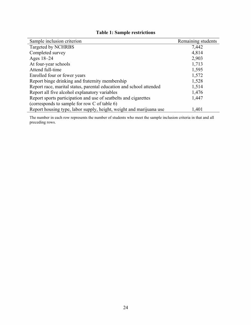
Table 1: Sample restrictions

Sample inclusion criterion Remaining students Targeted by NCHRBS 7,442 Completed survey 4,814 Ages 18–24 2,903 At four-year schools 1,713 Attend full-time 1,595 Enrolled four or fewer years 1,572 Report binge drinking and fraternity membership 1,528 Report race, marital status, parental education and school attended 1,514 Report all five alcohol explanatory variables 1,476 Report sports participation and use of seatbelts and cigarettes (corresponds to sample for row C of table 6)

1,447

Report housing type, labor supply, height, weight and marijuana use 1,401

The number in each row represents the number of students who meet the sample inclusion criteria in that and all preceding rows.

24

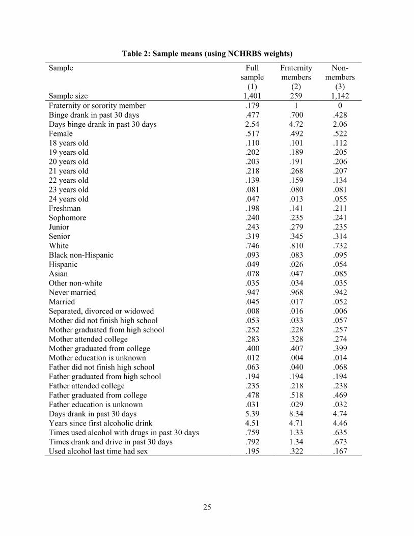
Table 2: Sample means (using NCHRBS weights)

Sample Full sample

Fraternity members

Non-members

(1) (2) (3) Sample size 1,401 259 1,142 Fraternity or sorority member .179 1 0 Binge drank in past 30 days .477 .700 .428 Days binge drank in past 30 days 2.54 4.72 2.06 Female .517 .492 .522 18 years old .110 .101 .112 19 years old .202 .189 .205 20 years old .203 .191 .206 21 years old .218 .268 .207 22 years old .139 .159 .134 23 years old .081 .080 .081 24 years old .047 .013 .055 Freshman .198 .141 .211 Sophomore .240 .235 .241 Junior .243 .279 .235 Senior .319 .345 .314 White .746 .810 .732 Black non-Hispanic .093 .083 .095 Hispanic .049 .026 .054 Asian .078 .047 .085 Other non-white .035 .034 .035 Never married .947 .968 .942 Married .045 .017 .052 Separated, divorced or widowed .008 .016 .006 Mother did not finish high school .053 .033 .057 Mother graduated from high school .252 .228 .257 Mother attended college .283 .328 .274 Mother graduated from college .400 .407 .399 Mother education is unknown .012 .004 .014 Father did not finish high school .063 .040 .068 Father graduated from high school .194 .194 .194 Father attended college .235 .218 .238 Father graduated from college .478 .518 .469 Father education is unknown .031 .029 .032 Days drank in past 30 days 5.39 8.34 4.74 Years since first alcoholic drink 4.51 4.71 4.46 Times used alcohol with drugs in past 30 days .759 1.33 .635 Times drank and drive in past 30 days .792 1.34 .673 Used alcohol last time had sex .195 .322 .167

25

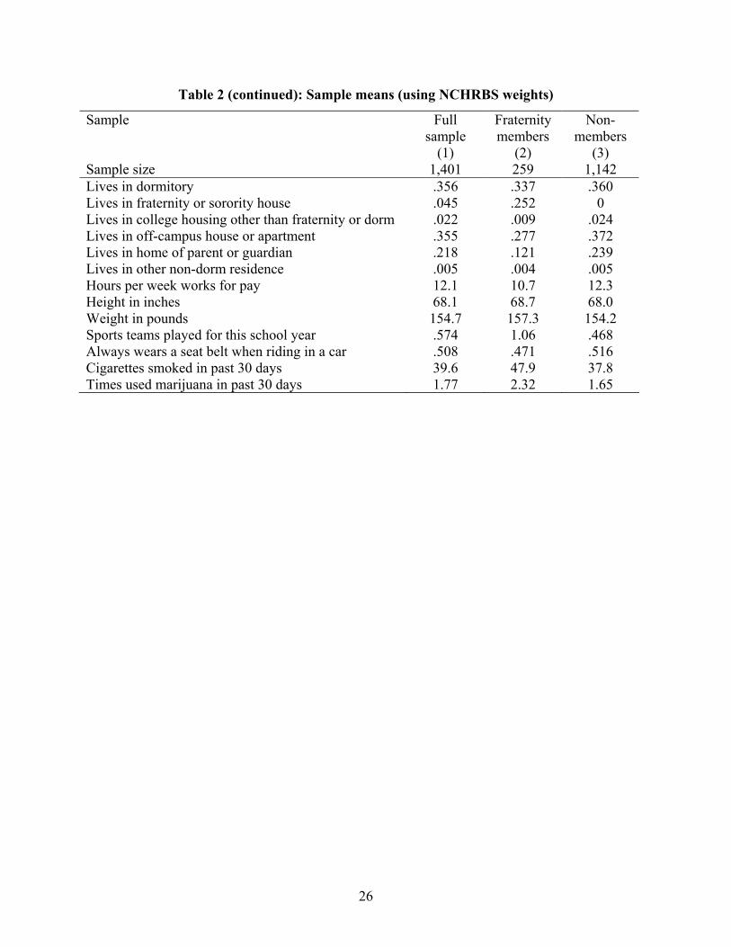
Table 2 (continued): Sample means (using NCHRBS weights)

Sample Full sample

Fraternity members

Non-members

(1) (2) (3) Sample size 1,401 259 1,142 Lives in dormitory .356 .337 .360 Lives in fraternity or sorority house .045 .252 0 Lives in college housing other than fraternity or dorm .022 .009 .024 Lives in off-campus house or apartment .355 .277 .372 Lives in home of parent or guardian .218 .121 .239 Lives in other non-dorm residence .005 .004 .005 Hours per week works for pay 12.1 10.7 12.3 Height in inches 68.1 68.7 68.0 Weight in pounds 154.7 157.3 154.2 Sports teams played for this school year .574 1.06 .468 Always wears a seat belt when riding in a car .508 .471 .516 Cigarettes smoked in past 30 days 39.6 47.9 37.8 Times used marijuana in past 30 days 1.77 2.32 1.65

26

Table 3: Effects on binge drinking with only exogenous covariates

Any binge drinking in past 30 days

Days of binge drinking in past 30 days

(1) (2) (3) (4) (5) (6) Fraternity or sorority member

.271 (7.40) .568

.222 (6.90) .466

.228 (7.16) .478

2.12 (7.56) .835

1.66 (7.17) .653

1.72 (7.19) .679

Female –.127 (4.85)

–.114 (4.50)

–1.08 (5.82)

–.979 (5.40)

18 years old .084 (1.21)

.020 (0.30)

–.339 (0.60)

–.533 (1.00)

19 years old .080 (1.46)

.045 (0.85)

–.142 (0.32)

–.247 (0.61)

20 years old .077 (1.77)

.056 (1.33)

–.069 (0.20)

–.128 (0.38)

22 years old –.002 (0.04)

.029 (0.65)

–.153 (0.42)

.055 (0.16)

23 years old .063 (1.05)

.090 (1.50)

.362 (0.81)

.569 (1.30)

24 years old –.011 (0.15)

.052 (0.73)

–.682 (1.39)

–.258 (0.53)

Freshman –.039 (0.60)

.042 (0.66)

.279 (0.52)

.502 (1.07)

Sophomore –.008 (0.14)

.058 (1.17)

.085 (0.22)

.294 (0.81)

Junior –.030 (0.73)

.005 (0.13)

–.027 (0.09)

.166 (0.56)

Black non-Hispanic –.363 (7.98)

–.299 (5.51)

–2.73 (6.96)

–2.40 (5.27)

Hispanic –.125 (2.80)

–.124 (2.45)

–1.00 (2.97)

–.785 (2.00)

Asian –.402 (6.93)

–.374 (6.23)

–2.93 (6.13)

–2.76 (5.60)

Other non-white –.010 (0.14)

.044 (0.64)

–.515 (1.29)

–.161 (0.40)

Married –.338 (4.38)

–.270 (3.60)

–2.63 (4.28)

–2.17 (3.75)

Separated, divorced, widowed .210 (1.33)

.280 (1.44)

1.34 (1.27)

1.55 (1.35)

27

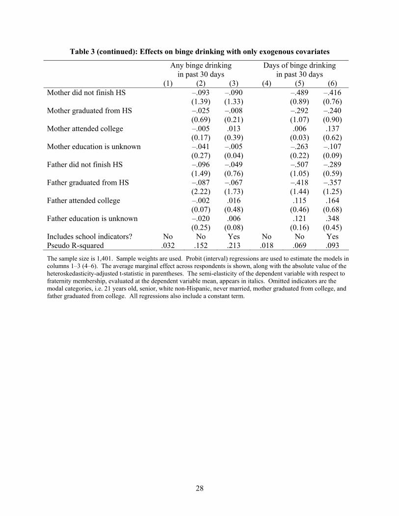
Table 3 (continued): Effects on binge drinking with only exogenous covariates Any binge drinking

in past 30 days Days of binge drinking

in past 30 days (1) (2) (3) (4) (5) (6) Mother did not finish HS –.093

(1.39) –.090 (1.33)

–.489 (0.89)

–.416 (0.76)

Mother graduated from HS –.025 (0.69)

–.008 (0.21)

–.292 (1.07)

–.240 (0.90)

Mother attended college –.005 (0.17)

.013 (0.39)

.006 (0.03)

.137 (0.62)

Mother education is unknown –.041 (0.27)

–.005 (0.04)

–.263 (0.22)

–.107 (0.09)

Father did not finish HS –.096 (1.49)

–.049 (0.76)

–.507 (1.05)

–.289 (0.59)

Father graduated from HS –.087 (2.22)

–.067 (1.73)

–.418 (1.44)

–.357 (1.25)

Father attended college –.002 (0.07)

.016 (0.48)

.115 (0.46)

.164 (0.68)

Father education is unknown –.020 (0.25)

.006 (0.08)

.121 (0.16)

.348 (0.45)

Includes school indicators? No No Yes No No Yes Pseudo R-squared .032 .152 .213 .018 .069 .093

The sample size is 1,401. Sample weights are used. Probit (interval) regressions are used to estimate the models in columns 1–3 (4–6). The average marginal effect across respondents is shown, along with the absolute value of the heteroskedasticity-adjusted t-statistic in parentheses. The semi-elasticity of the dependent variable with respect to fraternity membership, evaluated at the dependent variable mean, appears in italics. Omitted indicators are the modal categories, i.e. 21 years old, senior, white non-Hispanic, never married, mother graduated from college, and father graduated from college. All regressions also include a constant term.

28

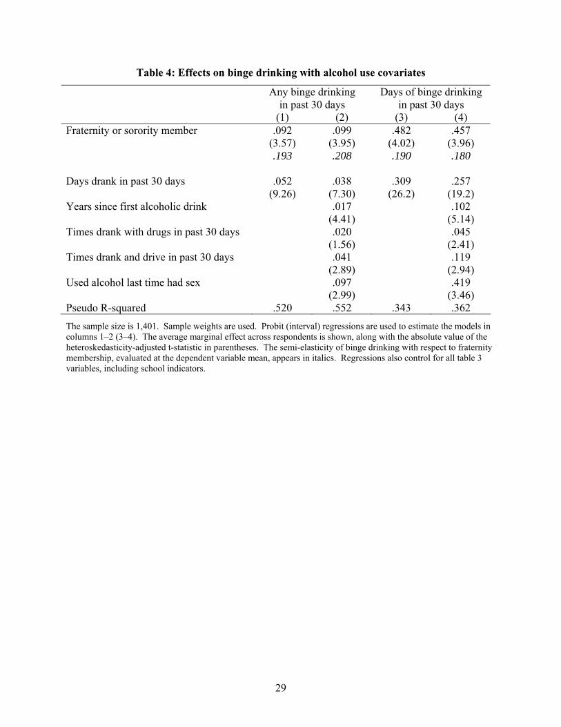
Table 4: Effects on binge drinking with alcohol use covariates

Any binge drinking in past 30 days

Days of binge drinking in past 30 days

(1) (2) (3) (4) Fraternity or sorority member

.092 (3.57) .193

.099 (3.95) .208

.482 (4.02) .190

.457 (3.96) .180

Days drank in past 30 days

.052 (9.26)

.038 (7.30)

.309 (26.2)

.257 (19.2)

Years since first alcoholic drink

.017 (4.41)

.102 (5.14)

Times drank with drugs in past 30 days

.020 (1.56)

.045 (2.41)

Times drank and drive in past 30 days

.041 (2.89)

.119 (2.94)

Used alcohol last time had sex

.097 (2.99)

.419 (3.46)

Pseudo R-squared .5 0 2 .552 .343 .362

The sample size is 1,401. Sample weights are used. Probit (interval) regressions are used to estimate the models in columns 1–2 (3–4). The average marginal effect across respondents is shown, along with the absolute value of the heteroskedasticity-adjusted t-statistic in parentheses. The semi-elasticity of binge drinking with respect to fraternity membership, evaluated at the dependent variable mean, appears in italics. Regressions also control for all table 3 variables, including school indicators.

29

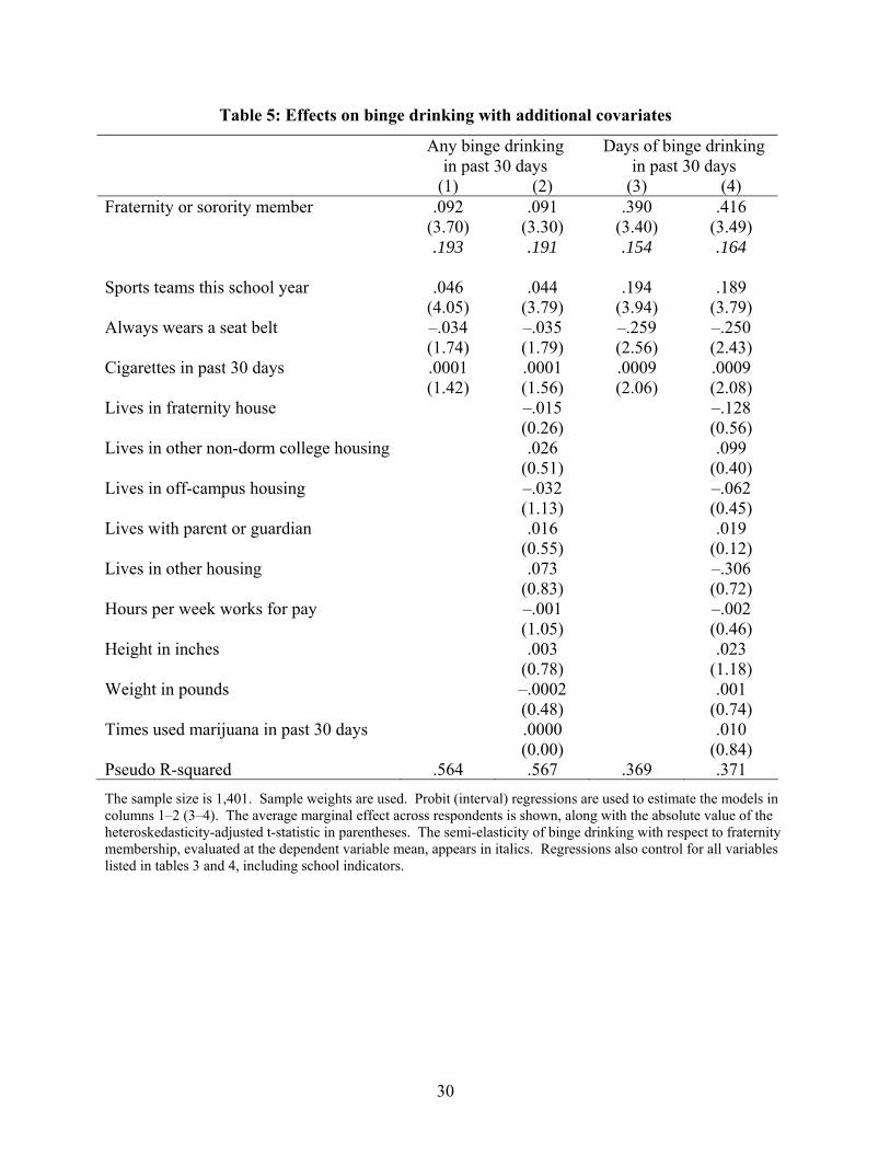
Table 5: Effects on binge drinking with additional covariates

Any binge drinking in past 30 days

Days of binge drinking in past 30 days

(1) (2) (3) (4) Fraternity or sorority member

.092 (3.70) .193

.091 (3.30) .191

.390 (3.40) .154

.416 (3.49) .164

Sports teams this school year

.046 (4.05)

.044 (3.79)

.194 (3.94)

.189 (3.79)

Always wears a seat belt

–.034 (1.74)

–.035 (1.79)

–.259 (2.56)

–.250 (2.43)

Cigarettes in past 30 days

.0001 (1.42)

.0001 (1.56)

.0009 (2.06)

.0009 (2.08)

Lives in fraternity house

–.015 (0.26)

–.128 (0.56)

Lives in other non-dorm college housing .026 (0.51)

.099 (0.40)

Lives in off-campus housing

–.032 (1.13)

–.062 (0.45)

Lives with parent or guardian

.016 (0.55)

.019 (0.12)

Lives in other housing .073 (0.83)

–.306 (0.72)

Hours per week works for pay

–.001 (1.05)

–.002 (0.46)

Height in inches

.003 (0.78)

.023 (1.18)

Weight in pounds

–.0002 (0.48)

.001 (0.74)

Times used marijuana in past 30 days .0000 (0.00)

.010 (0.84)

Pseudo R-squared .5 4 6 .567 .369 .371

The sample size is 1,401. Sample weights are used. Probit (interval) regressions are used to estimate the models in columns 1–2 (3–4). The average marginal effect across respondents is shown, along with the absolute value of the heteroskedasticity-adjusted t-statistic in parentheses. The semi-elasticity of binge drinking with respect to fraternity membership, evaluated at the dependent variable mean, appears in italics. Regressions also control for all variables listed in tables 3 and 4, including school indicators.

30

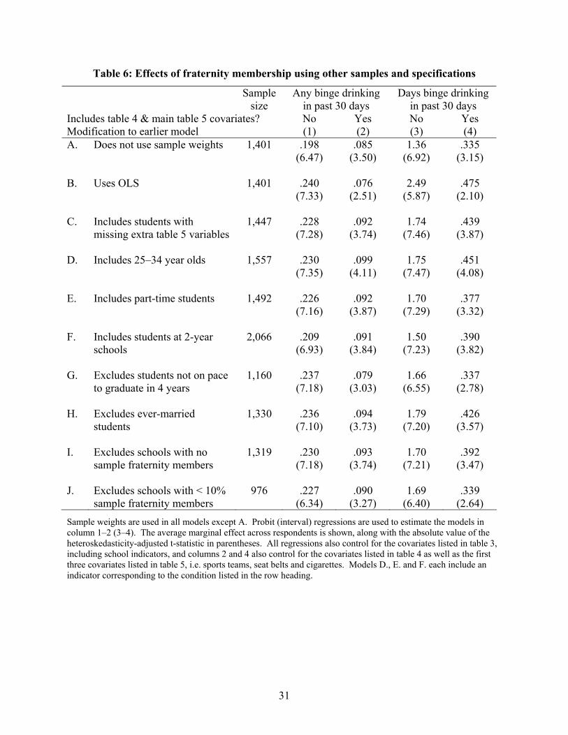
Table 6: Effects of fraternity membership using other samples and specifications

Sample size

Any binge drinking in past 30 days

Days binge drinking in past 30 days

Includes table 4 & main table 5 covariates? No Yes No Yes Modification to earlier model (1) (2) (3) (4) A. Does not use sample weights

1,401 .198 (6.47)

.085 (3.50)

1.36 (6.92)

.335 (3.15)

B. Uses OLS

1,401 .240 (7.33)

.076 (2.51)

2.49 (5.87)

.475 (2.10)

C. Includes students with missing extra table 5 variables

1,447 .228 (7.28)

.092 (3.74)

1.74 (7.46)

.439 (3.87)

D. Includes 25–34 year olds

1,557 .230 (7.35)

.099 (4.11)

1.75 (7.47)

.451 (4.08)

E. Includes part-time students

1,492 .226 (7.16)

.092 (3.87)

1.70 (7.29)

.377 (3.32)

F. Includes students at 2-year schools

2,066 .209 (6.93)

.091 (3.84)

1.50 (7.23)

.390 (3.82)

G. Excludes students not on pace to graduate in 4 years

1,160 .237 (7.18)

.079 (3.03)

1.66 (6.55)

.337 (2.78)

H. Excludes ever-married students

1,330 .236 (7.10)

.094 (3.73)

1.79 (7.20)

.426 (3.57)

I. Excludes schools with no sample fraternity members

1,319 .230 (7.18)

.093 (3.74)

1.70 (7.21)

.392 (3.47)

J. Excludes schools with < 10% sample fraternity members

976 .227 (6.34)

.090 (3.27)

1.69 (6.40)

.339 (2.64)

Sample weights are used in all models except A. Probit (interval) regressions are used to estimate the models in column 1–2 (3–4). The average marginal effect across respondents is shown, along with the absolute value of the heteroskedasticity-adjusted t-statistic in parentheses. All regressions also control for the covariates listed in table 3, including school indicators, and columns 2 and 4 also control for the covariates listed in table 4 as well as the first three covariates listed in table 5, i.e. sports teams, seat belts and cigarettes. Models D., E. and F. each include an indicator corresponding to the condition listed in the row heading.

31

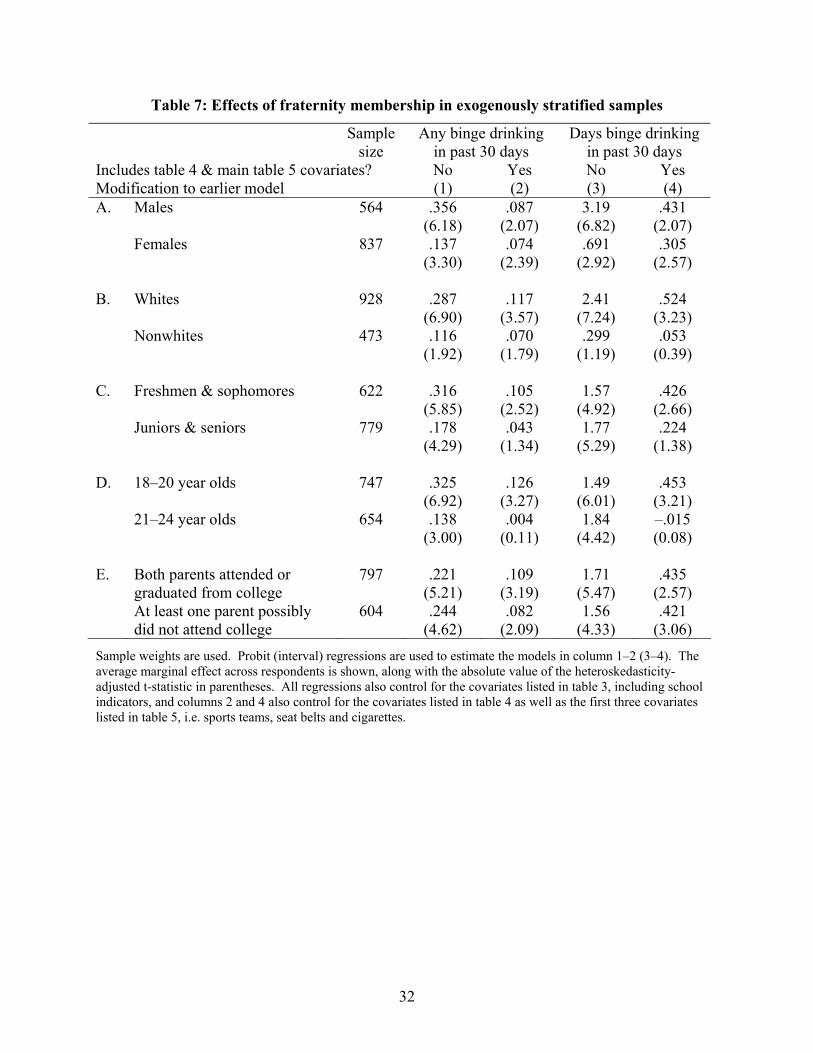
Table 7: Effects of fraternity membership in exogenously stratified samples

Sample size

Any binge drinking in past 30 days

Days binge drinking in past 30 days

Includes table 4 & main table 5 covariates? No Yes No Yes Modification to earlier model (1) (2) (3) (4) A. Males

564 .356

(6.18) .087

(2.07) 3.19

(6.82) .431

(2.07) Females

837 .137 (3.30)

.074 (2.39)

.691 (2.92)

.305 (2.57)

B. Whites 928 .287 (6.90)

.117 (3.57)

2.41 (7.24)

.524 (3.23)

Nonwhites

473 .116 (1.92)

.070 (1.79)

.299 (1.19)

.053 (0.39)

C. Freshmen & sophomores 622 .316 (5.85)

.105 (2.52)

1.57 (4.92)

.426 (2.66)

Juniors & seniors

779 .178 (4.29)

.043 (1.34)

1.77 (5.29)

.224 (1.38)

D. 18–20 year olds 747 .325 (6.92)

.126 (3.27)

1.49 (6.01)

.453 (3.21)

21–24 year olds

654 .138 (3.00)

.004 (0.11)

1.84 (4.42)

–.015 (0.08)

E. Both parents attended or graduated from college

797 .221 (5.21)

.109 (3.19)

1.71 (5.47)

.435 (2.57)

At least one parent possibly did not attend college

604 .244 (4.62)

.082 (2.09)

1.56 (4.33)

.421 (3.06)

Sample weights are used. Probit (interval) regressions are used to estimate the models in column 1–2 (3–4). The average marginal effect across respondents is shown, along with the absolute value of the heteroskedasticity-adjusted t-statistic in parentheses. All regressions also control for the covariates listed in table 3, including school indicators, and columns 2 and 4 also control for the covariates listed in table 4 as well as the first three covariates listed in table 5, i.e. sports teams, seat belts and cigarettes.

32