Free Material Optimization with FundamentalEigenfrequency Constraints∗

M. Stingl†, M. Kocvara‡ and G. Leugering§

October 28, 2008

Keywords. structural optimization, material optimization, semidefinite program-ming, nonlinear programming

AMS subject classifications. 74B05, 74P05, 90C90, 90C30, 90C22

AbstractThe goal of this paper is to formulate and solve free material optimization problemswith constraints on the smallest eigenfrequency of the optimal structure. A naturalformulation of this problem as linear semidefinite program turns out to be numericallyintractable. As an alternative, we propose a new approach, which is based on a non-linear semidefinite low-rank approximation of the semidefinite dual. We introduce analgorithm based on this approach and analyze its convergence properties. The article isconcluded by numerical experiments proving the effectiveness of the new approach.

1 IntroductionFree material optimization (FMO) is a branch of structural optimization that gains in-terest in the recent years. The underlying FMO model was introduced in [4] and hasbeen studied in several further articles as, for example, [2, 30]. The design variable inFMO is the full elastic stiffness tensor that can vary from point to point. The method issupported by powerful optimization and numerical techniques which allow for scenar-ios with complex bodies, fine finite-element meshes and several load cases. FMO hasbeen successfully used for conceptual design of aircraft components; the most promi-nent example is the design of ribs in the leading edge of Airbus A380 [13].

As mentioned, the optimal elastic stiffness tensor can vary from point to point; itshould be physically available but is otherwise not restricted. Given this freedom, wehave to face the question of interpretation of the optimal result. A general anisotropic∗This work was partly supported by the EU Commission in the Sixth Framework Program, Project

No. 30717 PLATO-N, and by grant A1075402 of the Czech Academy of Sciences (MK).†Institute of Applied Mathematics, University of Erlangen, Martensstr. 3, 91058 Erlangen, Germany

(stingl@am.uni-erlangen.de)‡School of Mathematics, University of Birmingham, Edgbaston Birmingham B15 2TT, UK, and In-

stitute of Information Theory and Automation, Pod vodarenskou vezi 4, 18208 Praha 8, Czech Republic(kocvara@maths.bham.ac.uk)§Institute of Applied Mathematics, University of Erlangen, Martensstr. 3, 91058 Erlangen, Germany

(leugering@am.uni-erlangen.de)

1

material that changes its properties at any point is certainly not easy to manufac-ture. The most natural interpretation is the use of fibre-reinforced composite materials,though other interpretations are possible, too. The problem gives the best physicallyattainable material and its result thus serves as a benchmark to any realized design. Thequestion of practical interpretation of FMO results is intensively studied in the recentEU FP6 project PLATO-N, whose consortium includes several industrial partners.

The basic FMO model has other drawbacks, though. For example, structures mayfail due to high stresses, or due to lack of stability of the optimal structure (compare[16, 17] for further discussion). In order to prevent this undesirable behavior, addi-tional requirements have to be taken into account in the FMO model. Typically, suchmodifications lead to additional constraints on the set of admissible materials and/orthe set of admissible displacements. These constraints usually destroy the favorablemathematical structure of the original problem (see [16, 17]). The particular cause ofstructural failure we want to investigate in this article is vibration resonance. Structuraloptimization problems with eigenvalue constraints have been intensively studied in thecontext of truss and topology optimization, see, e.g., [9, 10, 20, 22, 23, 24] and manyothers. We will give an appropriate formulation of the FMO problem, which takes careof this phenomenon, derive various discretized formulations and propose an efficientalgorithm for the solution of the problem.

In contrast to the original FMO model which is based on a static PDE system, vibra-tion of a body is a dynamic process. In the first part of the paper we demonstrate howwe can bypass this additional challenge by using a reformulation as (time-independent)generalized eigenvalue problem. As a result, we obtain an extended FMO problem withan eigenfrequency condition. For this problem we are able to prove the existence ofan optimal solution. In the second section we explain how an existing discretizationscheme (proposed in [28]) can be extended to cover the additional eigenfrequency con-dition. In the third section we give a first formulation of the discretized FMO problemwith vibration constraint as a linear semidefinite program. We further explain whythis formulation is not suited to serve as a basis for efficient numerical calculations.In the framework of the fourth section we develop an algorithm which is based on alow-rank approximation of the semidefinite dual. The low-rank approach is motivatedby ideas recently introduced by Burer and Monteiro (see [6]) for the solution of linearsemidefinite programs. The article is concluded by numerical studies.

Throughout this article we use the following notation: We denote by SN the spaceof symmetric N×N matrices equipped with the standard inner product 〈·, ·〉 definedby 〈A,B〉 := Tr(AB) for any pair of matrices A,B ∈ SN . We further denote by SN+the cone of all positive semidefinite matrices in SN and use the abbreviation A < 0for matrices A ∈ SN+ . Moreover, for A,B ∈ SN , we say that A < B if and only ifA−B < 0, and similarly for A 4 B.

2 The mathematical modelMaterial optimization deals with optimal design of elastic structures, where the designvariables are material properties. The material can even vanish in certain areas, thusthe so-called topology optimization (see, e.g., [3]) can be considered a special case ofmaterial optimization.

Let Ω ⊂ R2 be a two-dimensional bounded domain1 with a Lipschitz boundary.

1The entire presentation is given for two-dimensional bodies, to keep the notation simple. Extension tothe three-dimensional space is straightforward.

2

By u(x) = (u1(x), u2(x)) we denote the displacement vector at a point x of the bodyunder load f , and by

eij(u(x)) =12

(∂ui(x)∂xj

+∂uj(x)∂xi

)for i, j = 1, 2

the (small-)strain tensor. We assume that our system is governed by linear Hooke’slaw, i.e., the stress is a linear function of the strain

σij(x) = Eijk`(x)ek`(u(x)) (in tensor notation),

where E is the elastic (plane-stress) stiffness tensor. The symmetries of E allow us towrite the 2nd order tensors e and σ as vectors

e = (e11, e22,√

2e12)> ∈ R3, σ = (σ11, σ22,√

2σ12)> ∈ R3 .

Correspondingly, the 4th order tensor E can be written as a symmetric 3× 3 matrix

E =

E1111 E1122

√2E1112

E2222

√2E2212

sym. 2E1212

. (1)

In this notation, Hooke’s law reads as σ(x) = E(x)e(u(x)).For a given external load function f ∈ [L2(Γ)]2 we obtain the following basic

boundary value problem of linear elasticity:

Find u ∈ [H1(Ω)]2 such that (2)

div(σ) = 0 in Ωσ · n = f on Γu = 0 on Γ0

σ = E · e(u) in Ω

Here Γ and Γ0 are open disjunctive subsets of ∂Ω. The corresponding weak form,the so called weak equilibrium equation, reads as:

Find u ∈ V, such that (3)∫Ω

〈E(x)e(u(x)), e(v(x))〉dx =∫

Γ

f(x) · v(x)dx, ∀v ∈ V,

where V = u ∈ [H1(Ω)]2 |u = 0 on Γ0 ⊃ [H10 (Ω)]2 reflects the Dirichlet boundary

conditions. Below we will use the abbreviation

aE(w, v) =∫

Ω

〈E(x)e(w(x)), e(v(x))〉dx (4)

for the bilinear form on the left hand side of (3). In free material optimization (FMO),the design variable is the elastic stiffness tensor E which is a function of the spacevariable x (see [4]). The only constraint on E is that it is physically reasonable, i.e.,thatE is symmetric and positive semidefinite. This gives rise to the following definition

E0 :=E ∈ L∞(Ω)3×3 | E = E>, E < 0 a.e. in Ω

.

The choice of L∞ is due to the fact that we want to allow for material/no-materialsituations. A frequently used measure of the stiffness of the material tensor is its trace.

3

In order to avoid arbitrarily stiff material, we add pointwise stiffness restrictions of theform Tr(E) ≤ ρ, where ρ is a finite real number. We also allow for pointwise lowertrace bounds Tr(E) ≥ ρ ≥ 0. Moreover we prescribe the total stiffness/volume bythe constraint v(E) = v. Here the volume v(E) is defined as

∫Ω

Tr(E)dx and v ∈ Ris an upper bound on overall resources. Accordingly, we define the set of admissiblematerials as

E :=E ∈ E0 | ρ ≤ Tr(E) ≤ ρ a.e. in Ω, v(E) = v

.

We are now able to present the minimum compliance single-load FMO problem

infE∈E

∫Γ

f(x) · uE(x)dx (5)

subject touE solves (3).

The objective, the so called compliance functional, measures how well the structurecan carry the load f . In [28] it is shown that problem (5) can be given equivalently as

infE∈E

c(E)

where c(E) is a closed formula for the compliance given by

c(E) = supu∈V

−aE(u, u) + 2

∫Γ

f · u dx.

Problem (5) has been extensively studied in [18, 28]. The most successful methodfor the solution of problem (5), based on dualization of the original problem [2, 28]gave rise to a software package MOPED, which was recently applied to real-worldapplications and lead to significant improvements of the classic design. On the otherhand the underlying FMO model has certain limitations (other than the interpretationof the result discussed in the introduction). One of the drawbacks of problem (5) isthat it does not count with possible instability of the structure (compare [16]). Onepossible source of such instability is vibration resonance. In the sequel we develop ageneralized FMO model, which is more robust with respect to this phenomenon. Aswe will see, the modification in the model results in an additional constraint on the setof admissible materials E .

Vibration of a body—as a dynamic process—can be modeled by the followingtime-dependent PDE:

div(σ(x, t)) = ρE(x)u(x, t), (x, t) ∈ Ω× [0, T ], (6)

with boundary conditions

∂

∂nσ(x, t) = 0 on Γ× [0, T ]

u(x, t) = 0 on Γ0 × [0, T ].

Here the material density term ρ is defined by ρE(x) = tr(E(x)) and E(x) is the ma-terial tensor introduced earlier in this section. As in this case there is no external force

4

applied to the system, we call the solutions of (6) free vibrations. Using the assump-tion of Hooke’s law and introducing the differential operator SE(·) := div(Ee(·)) weobtain from (6):

SE(u(x, t)) = ρE(x)u(x, t), (x, t) ∈ Ω× [0, T ], (7)∂

∂nSE(u(x, t)) = 0 on Γ× [0, T ],

u(x, t) = 0 on Γ0 × [0, T ].

Using Fourier transform we derive the following characterization of solutions of system(7):

Proposition 2.1. The solutions of system (7) are of the form

u(x, t) =∞∑j=1

[aj cos(

√λjt) + bj sin(

√λjt)

]wj(x), (8)

where aj , bj , are free real parameters and λj , wj are the solutions (eigenvalues andeigenvectors, respectively) of the generalized eigenvalue problem

−SE(wj(x)) = λjρE(x)wj(x), x ∈ Ω (9)∂

∂nσ(x) = 0 on Γ

u(x) = 0 on Γ0.

Introducing the bilinear form

b(w, v) =∫

Ω

m(x)w(x)v(x)dx,

the weak form associated with (9) is:

Find λ ∈ R, u ∈ V, u 6= 0, such that : aE(u, v) = λb(u, v) ∀v ∈ V. (10)

In the standard dynamic analysis of a structure with a given isotropic material, themultiplier m(x) in the definition of the bilinear form b has a meaning of the mass.In the following, we will relate it to the trace of the elasticity matrix. We follow thediscussion in [3] and assume that, for a given E, the mass belongs toM(E), a set ofall materials with the same elastic properties but different mass, i.e., m ∈ M(E) =m(τ) | E(τ) = E . The tensorE is uniquely characterized by its principal invariants(up to a rotation that does not affect the mass), so we may write m ∈ M(I1, I2, I3). Itwas shown in [3] that when we maximize the smallest eigenvalue subject to the volumeconstraint only (with no compliance constraint), the optimal material satisfies I2 =I3 = 0. In our case, we will assume this, so we will have that m ∈ MρE(x). Further,motivated by the isotropic case, we will assume that m is in fact a linear function ofthe first invariant, i.e., m(x) = c(x)ρE(x), cx,E ≤ c(x) ≤ cx,E . Finally, we willassume that the constant c is independent of x, which corresponds to the assumptionthat the optimal structure is made of the “same kind of material”. This, certainly, is asimplification that needs to be taken into account in the interpretation of the results. Inthe rest of the paper we will thus use the following form of b:

b(w, v) := bE(w, v) =∫

Ω

cρE(x)w(x)v(x)dx,

with certain c > 0.We use the following definition of the smallest well defined eigenvalue.

5

Definition 2.2. For each E ∈ E0, let λmin(E) denote the smallest well defined eigen-value of the system (10), i.e.

λmin = min λ | ∃u ∈ V : Equation (10) holds for (λ, u) and u /∈ ker(bE) ,

whereker(bE) = z | bE(z, v) = 0 ∀v ∈ V.

The square root of the smallest well-defined eigenvalue will be called fundamentaleigenfrequency.

It is well known from engineering literature that the dynamic stiffness of a structurecan be improved by raising its fundamental eigenfrequency. This is our motivationfor considering the following problem: We search for a material distribution E suchthat the smallest well defined eigenvalue of the system (10) is larger than a prescribedpositive lower bound. Denoting this value by λ, we obtain the constraint

λmin(E) ≥ λ. (11)

In Appendix A, Corollary A.3 it is shown that inequality (11) can be equivalently re-formulated as

infu∈V,‖u‖=1

aE(u, u)− λbE(u, u)

≥ 0. (12)

Introducing the function

µλ : L∞(Ω)3×3 → R ∪ ∞

E 7→ infu∈V,‖u‖=1

aE(u, u)− λbE(u, u)

,

we are able to state the minimum compliance single-load FMO problem with vibrationconstraint

infE∈E

∫Γ

f(x) · uE(x)dx (13)

subject touE solves (3) ,µλ(E) ≥ 0 .

Next we want to investigate the well-posedness of problem (13). We start with thefollowing lemma:

Lemma 2.3. The function µλ is upper semicontinuous and concave.

Proof. We first note that for fixed u ∈ V the mapping E 7→ aE(u, u) − λbE(u, u)is affine and consequently continuous w. r. t. E. Consequently, µλ is the infimum ofaffine functionals and thus concave. Moreover, µλ is upper semicontinuous, as it is theinfimum of (infinitely many) continuous functionals [11, Proposition III.1.2].

Using Lemma 2.3 we are able to give details about the structure of the feasible setof problem (13):

Lemma 2.4. The set E λ =E ∈ E | µλ ≥ 0

is weakly-∗ compact.

6

Proof. The weakly-∗ compactness of E has been shown in the proof of Theorem 2.1in [2]. Thus the only thing we have to show is that E λ is closed. But this followsimmediately from the closedness of E and Lemma 2.3.

The following theorem can be proved exactly in the same way as Theorem 2.1 in[2]:

Theorem 2.5. If the set E λ is non-empty, then problem (13) has at least one solution.

We conclude this section by two remarks.

Remark 2.6. From the equivalence of (11) and (12) and Lemma 2.4 we immediatelyconclude that the function λmin : L∞(Ω)3×3 → R ∪ ∞ is upper semicontinuousand quasiconcave. Using this and the fact that the compliance functional, given by theformula

c(E) = supu∈V

−1

2aE(u, u) +

∫Γ

f · u dx

is convex and lower semicontinuous w. r. t. E (see [28]), we may repeat the argumentsabove in order to verify existence of at least one optimal solution for the followingproblems:

infE∈E

v(E) (14)

subject toc(E) ≤ δ,

λmin ≥ λ .

and

infE∈E−λmin(E) (15)

subject toc(E) ≤ δ,v(E) = v .

Here δ ∈ R is an upper bound on the compliance of the structure.

Remark 2.7. All results presented above remain true when we consider more generalDirichlet boundary conditions of the form

ui = 0 on Γ0 for i = 1 and/or 2.

3 DiscretizationIn order to solve the infinite-dimensional problem (13) numerically, we have to use anappropriate discretization scheme. For the discretization, we use the standard isoparatem-ric concept (see, e.g., [8]), using a piecewise constant approximation of the matrix func-tion E(x) and a piece-wise linear approximation of the displacements u(x). Ratherthan presenting the full convergence analysis, we just note that the finite element ap-proach and convergence analysis presented in [28] applies to our problem without

7

changes and which generalizes the analysis presented in [25] for the variable thick-ness problems.

To keep the notation simple, we use the same symbols for the discrete objects (vec-tors) as for the “continuum” ones (functions). Suppose that Ω is approximated by a par-titioning of M quadrilaterals called Ωi. Let us denote by n the number of nodes (ver-tices of the elements). We approximate the matrix function E(x) by a function that isconstant on each element, i.e., characterized by a tuple of matrices E = (E1, . . . , EM )of its element values. Hence the discrete counterpart of the set of admissible materialsin algebraic form is

E =

E ∈ (S3)M | Ei < 0, ρ ≤ Tr(Ei) ≤ ρ, i = 1, . . . ,M,

M∑i=1

Tr(Ei) = v

.

(16)Here v is derived from the upper bound on resources introduced in (5) and the measureof a single element ω. Further we assume that the displacement vector u(x) is approx-imated by a continuous function that is bilinear in each coordinate on every element.Such a function can be written as u(x) =

∑ni=1 uiϑi(x) where ui is the value of u at

ith node and ϑi is the basis function associated with ith node (for details, see [8]). Re-call that the displacement function is vector valued with 2 components. Consequentlyany function in the discrete set of admissible displacements can be identified with avector in RN , where N = 2n − #(components of u fixed by Dirichlet b. c.) and weobtain

V = RN . (17)

With the (reduced) family of basis functions ϑk, k = 1, 2, . . . , N , we define the3× 2 matrix

B>k =

∂ϑk∂x1

0 12∂ϑk∂x2

0 ∂ϑk∂x2

12∂ϑk∂x1

.

Now, for an element Ωi, let Di be an index set of nodes belonging to this element.Next we want to derive the discrete counter part of aE(·, ·). We use a Gauss formulafor the evaluation of the integral over each element Ωi, assume that there are G Gaussintegration points on each element and denote by xGi,k the k-th integration point on thei-th element. Next we construct block matrices Bi,k ∈ R3×N composed of (3 × 2)blocks Bj(xGi,k), at j-th position for all j ∈ Di and zero blocks otherwise. Then thediscrete counterpart of aE(·, ·), the stiffness matrix is

A(E) =M∑i=1

Ai(E), Ai(E) =G∑k=1

B>i,kEiBi,k . (18)

The matricesAi ∈ RN×N are usually called element stiffness matrices. Now, assumingthe load function f to be linear on each element and identifying such a function with avector f ∈ RN , the discrete objective functional and equilibrium condition read as

f>u, A(E)u = f, (19)

respectively. Similarly, we use the representation of the discrete displacement functionsin the basis of ϑk, k = 1, 2, . . . , N , to derive the discrete version of the bilinear form

8

bE(·, ·): defining vectors Vi,k ∈ RN , i = 1, 2, . . . ,M, k = 1, 2, . . . , G, with ϑj(xki ),j ∈ Di at j-th position and zeros otherwise, the mass matrix is given by

M(E) =M∑i=1

Mi(E), Mi(E) = Tr(E)Mi, Mi =G∑k=1

Vi,kV>i,k . (20)

As in (18), M(E) is composed by a sum of matrices Mi ∈ RN×N , the element massmatrices. Finally, the discrete counterpart of the condition on the lowest eigenfre-quency of the structure (12) reads as

infu∈Rn,‖u‖=1

u>(A(E)− λM(E)

)u ≥ 0. (21)

After discretization, problem (13) becomes

minu∈RN ,E∈E

f>u (22)

subject toA(E)u = f,

infu∈Rn,‖u‖=1

u>(A(E)− λM(E)

)u ≥ 0 .

Problem (22) is a mathematical programming problem with linear matrix inequalityconstraints and standard nonlinear constraints; in the following section we will showhow this problem can be turned into a standard linear semidefinite program.

4 The linear SDP approachIn the recent years excellent software packages, most of them based on the interior pointidea, have been developed for the solution of linear SDP problems. For an overview,compare, for example, [29] or [19].

In the sequel we give an alternative formulation of the discrete FMO problem (22)as linear semidefinite program.

Proposition 4.1. Problem (22) is equivalent to the following linear semidefinite pro-gram

minα∈R,E∈E

α (23)

subject to(α −f−f A(E)

)< 0

A(E)− λM(E) < 0 .

Proof. After introducing an auxiliary variable α, the assertion follows immediatelyfrom Proposition 3.1 in [1].

In the remainder of this section we will explain why the formulation as linear SDPis impractical for the efficient solution of FMO problems with vibration constraint, dueto the large number of variables and the size of the matrix constraints. Our observations

9

are based on practical experience and complexity estimates. We have solved Example1 from Section 7 by state-of-the-art linear SDP solvers. The fastest solver neededabout 50 hours on a high end computer with a processor speed of approximately 3GHz. Using this number as a reference and taking into account that the computationalcomplexity of all currently available linear SDP solvers depends at least quadratically(sometimes even cubically) on the size of the matrix constraints and typically cubicallyon the number of variables, it becomes obvious that formulation (23) is not suited toserve as a basis for the efficient solution of FMO problems of practical size.

Remark 4.2. Note that a formulation similar to (23) has been successfully applied toproblems of Truss Topology design as well as variable thickness sheet problems in thepast. The interested reader is referred to [22, 1, 16].

5 The dual problem and the low-rank approximationThe goal of this section is to find an alternative formulation to problem (23), which isnumerically tractable. Our strategy is as follows: First, we derive the Lagrange dual toproblem (23) and then present a low-rank approximation to the same, which is (undercertain assumptions) equivalent to the original problem.

The following theorem allows us to identify problem (23) as the Lagrange dual ofa convex semidefinite program:

Theorem 5.1. Problem (23) is equivalent to the Lagrange dual of the problem

maxu∈RN,α∈R,W<0,

βl≥0,βu≥0

2f>u− αV + ρ

M∑i=1

βli − ρM∑i=1

βui (24)

subject to

gi(u, α,W, βl, βu) 4 0, i = 1, 2, . . . ,M,

where gi(u, α,W, βl, βu) : RN+1×SN×R2M 7→ S3 is defined for all i = 1, 2, . . . ,Mas

gi(u, α,W, βl, βu)

=G∑j=1

B>ijuu>Bij +

G∑j=1

B>ijWBij − λ〈W,Mi〉I −(α+ βli − βui

)I.

Moreover there is no duality gap and the optimal material matrices

E∗i , i = 1, 2, . . . ,M

take the role of Lagrangian multipliers associated with the nonlinear inequality con-straints in problem (24).

Proof. We will prove the theorem for formulation (22) which, by Proposition 4.1, isequivalent to (23). Rewriting the eigenfrequency constraints as in problem (23) andtaking into account that A(E) is positive definite for all E ∈ E , we observe that prob-lem (22) can be written equivalently as

minE∈E

maxu∈RN

2f>u− u>A(E)u (25)

subject to

A(E)− λM(E) < 0 .

10

The Lagrangian associated with problem (25) can be written in the form

L(E, u, α,W, βl, βu) := maxu∈RN

2f>u− u>A(E)u (26)

+M∑i=1

βli(ρ− Tr(Ei)) +M∑i=1

βui (Tr(Ei)− ρ)

+ α(M∑i=1

Tr(Ei)− V ) + 〈W, λM(E)−A(E)〉,

where(E, u, α,W, βl, βu) ∈ (Sd

′

+ )M × RN × R× SN+ × RM+ × RM+ .

Now problem (25) can be formulated as

minE<0

maxu∈RN,α∈R,W<0,

βl≥0,βu≥0

L(E, u, α,W, βl, βu). (27)

The Lagrange dual to (27) is

maxu∈RN,α∈R,W<0,

βl≥0,βu≥0

minE<0L(E, u, α,W, βl, βu). (28)

Taking into account that

u>A(E)u = u>( M∑i=1

G∑j=1

BijEiB>ij

)u =

M∑i=1

⟨Ei,

G∑j=1

B>ijuu>Bij

⟩

〈W,A(E)〉 =⟨W,

M∑i=1

G∑j=1

BijEiB>ij

⟩=

M∑i=1

⟨Ei,

G∑j=1

B>ijWBij

⟩

〈W,M(E)〉 =⟨W,

M∑i=1

Tr(Ei)Mi

⟩=

M∑i=1

〈Ei, I〉〈W,Mi〉 =M∑i=1

⟨Ei, 〈W,Mi〉I

⟩and Tr(Ei) = 〈Ei, I〉 for all i = 1, 2, . . . ,M, we obtain

L(E, u, α,W, βl, βu) = 2f>u− αV + ρ

M∑i=1

βli − ρM∑i=1

βui

−M∑i=1

⟨Ei,

G∑j=1

B>ijuu>Bij +

G∑j=1

B>ijWBij − λ〈W,Mi〉I −(α+ βli − βui

)I⟩.

Using this form and interpretingEi (i = 1, 2, . . . ,M) as Lagrangian multipliers, prob-lem (28) takes the form

maxu∈RN,α∈R,W<0,

βl≥0,βu≥0

2f>u− αV + ρ

M∑i=1

βli − ρM∑i=1

βui

subject toG∑j=1

B>ij(uu> +W )Bij −

(λ〈W,Mi〉+ α+ βli − βui

)I 4 0, i = 1, 2, . . . ,M,

11

but this is problem (24). Finally, taking into account that problem (24) is convex andthat the Slater condition holds (in order to construct a strictly feasible point, use ar-bitrary W < 0, u ∈ RN , βl ≥ 0, βu ≥ 0 and choose α large enough, such that allinequalities in problem (24) are strictly feasible), the fact that the duality gap is zerofollows from [5, Theorem 5.81].

Later we will make use of the following proposition. The proof is straightforward,but rather technical and therefore postponed to Appendix I of this article.

Proposition 5.2. A tuple (u∗, α∗,W ∗, βl∗, βu

∗;E∗) ∈ RN+1 × SN+ ×R2M

+ × (S3+)M

is a KKT point of (24) if and only if the conditions

gi(u∗, α∗,W ∗, βl∗, βu

∗) 4 0 (i = 1, 2, . . . ,M)

ρ ≤ Tr(E∗i ) ≤ ρ (i = 1, 2, . . . ,M)

βl∗(ρ− Tr(E∗i )) = 0, βu

∗(Tr(E∗i )− ρ) = 0, (i = 1, 2, . . . ,M)∑M

i=1tr(E∗i ) = V, A(E∗)− λ∗M(E∗) < 0, 〈A(E∗)− λ∗M(E∗),W ∗〉 = 0

A(E∗)u∗ = f, f>u∗ = α∗V − ρ∑M

i=1βli + ρ

∑M

i=1βlu

are satisfied.

Theorem 5.1 guarantees that we can retrieve the solution of (22) by calculating aprimal-dual solution of (24). Consequently, we could apply any convex semidefiniteprogramming solver which is able to generate primal-dual solutions. Note, however,that the computational complexity of problem (24) is not much better than that of thelinear SDP problem (23). This is due to the large size of the positive semidefinitenessconstraint W < 0. For this reason, we follow the idea of Monteiro and Burer (see [6]),in order to construct a low-rank approximation of (24). Suppose for a moment that weknow a primal solution E∗ of problem (23). Then we define

R0 := dim(

ker(A(E∗)− λM(E∗)

)), (29)

which is equal to the dimension of the multiplicity of the smallest eigenvalue λ of thegeneralized eigenvalue problem A(E∗)v = λM(E∗)v. Now, assuming that Slater’scondition holds for (23), we observe that the matrix W in problem (24) takes the roleof the Lagrangian multiplier associated with the inequality constraint

A(E)− λM(E) < 0.

Moreover it follows from the complementarity slackness condition that there exists anoptimal multiplier W ∗, with the property

rank(W ∗) ≤ R0.

This is our motivation to substitute W in problem (24) by∑L`=1 w`w

>` with w` ∈ Rn

and with some L ∈ R. Doing this, we obtain

maxw1,w2,...,wL,u∈RN

α≥0,βl≥0,βu≥0

2f>u− αV + ρM∑i=1

βli − ρM∑i=1

βui (30)

subject to

gi(u, α,w1, w2, . . . , wL, βl, βu) 4 0, i = 1, . . . ,M,

12

where gi(u, α,w1, w2, . . . , wL, βl, βu) is defined as

G∑j=1

B>ij

(uu> +

L∑`=1

w`w>`

)Bij −

(λ⟨ L∑`=1

w`w>` ,Mi

⟩+ α+ βli − βui

)I

for all i = 1, 2, . . . ,M. The following theorem provides a relation between problems(24) and (30).

Theorem 5.3. Let E∗0 be a solution of (23) and R0 be defined by (29). Then thereexists L ≤ R0 such that for all (global) solutions

(u∗, α∗, w∗1 , . . . , w

∗L, β

l∗ , βu∗)

of(30) the tuple

(u∗, α∗,W ∗, βl

∗, βu

∗)with W ∗ :=

∑L`=1 w

∗` (w∗` )> is a solution of

(24). Moreover each vector of Lagrangian multipliers E∗ associated with the inequal-ity constraints

gi(u, α,w1, w2, . . . , wL, βl, βu) 4 0, i = 1, 2, . . . ,M,

forms an optimal solution of (23).

In order to proof Theorem 5.3, we make use of the following Lemmas:

Lemma 5.4. Any local/global minimum of problem (30) is a local/global minimum ofproblem (24) with an additional rank constraint of the form

rank(W ) ≤ L

and vice versa.

Proof. The assertion of Lemma 5.4 can be proven exactly in the same way as Proposi-tion 2.3 in [7].

Lemma 5.5. Robinson’s constraint qualification (see [5]) is satisfied by problem (30)at any feasible point.

Proof. Using [5, formula (5.195)] we can write Robinson’s constraint qualification foran arbitrary feasible point (u, α, w1, . . . , wL, βl, βu) ∈ R(L+1)N+2M+1 as follows:There exists a direction h ∈ R(L+1)N+2M+1 such that the inequality

gi(u, α, w1, . . . , wL, βl, βu) +∇gi(u, α, w1, . . . , wL, βl) · h ≺ 0 (31)

holds for all i = 1, 2, . . . ,M . Obviously, the direction (0, 1, 0, . . . , 0) with 1 in theposition of the variable α satisfies (31).

A simple consequence of Lemma 5.5 is that for each local minimum of problem(30) associated Lagrangian multipliers exist. Now we are able to prove Theorem 5.3:

Proof. Let L = R0 and x∗ :=(u∗, α∗, w∗1 , . . . , w

∗L, β

l∗ , βu∗)

be a (global) solutionof (30). Then we conclude from Lemma 5.4 that x∗ :=

(u∗, α∗,

∑w∗`w

∗>` , βl

∗, βu

∗)is a global solution of problem (24) with an additional rank constraint of the formrank(W ) ≤ L. But then we conclude from the definition of R0 that x∗ is a globalsolution of (24) (without any rank constraint). Moreover, Lemma 5.5 guarantees theexistence of optimal Lagrangian multipliers E∗ ∈ (S3

+)M associated with the inequal-ity constraints

gi(u, α,w1, w2, . . . , wL, βl, βu) 4 0, i = 1, 2, . . . ,M.

13

Now we define a Lagrangian-type function for problem (24) as follows:

L(x,E) =

f0(x) +

∑M

i=1〈Ei, gi(x)〉 x ∈ C, Ei < 0 (i = 1, 2, . . . ,M)

−∞ x ∈ C, Ei 6< 0 for some i−∞ x 6∈ C

where f0 is the objective of (24) and C is the convex set

C := RN+1 × SM+ × R2M+ .

As x∗ is a global solution of (24) and

L(x∗, E∗) = f0(x∗),

we conclude that (x∗, E∗) is a saddle point of L. Now we obtain for example from [26,Theorem 28.3] that E∗ is a solution of the dual problem to (24).

Theorem 5.3 allows us to replace problem (24) by a low-rank problem with an ap-propriate rank. The advantage of the low-rank problem is that the dimension of theoptimization variable is significantly lower than in the original problem, as long as themultiplicity of the smallest generalized eigenvalue of the stencil (A(E∗) | M(E∗)) isnot too large. Moreover, there is no large semidefinite constraint in the low-rank prob-lem. On the other hand, problem (30) is a non-convex semidefinite program, which canstill be considered large-scale. For such a problem it is generally difficult (if not impos-sible) to calculate a global solution. Even in the case a global solution has been found,it is not a trivial problem to detect globality. To cope with the first problem (findinga global optimum), from theoretical point of view, we cannot do much more than usean optimization algorithm with strong local convergence properties and provide a goodstart point. We will see in Section 7 that this is not a big problem in practice, as the lo-cal algorithm of our choice typically identifies the global optimum, provided our guessfor the multiplicity of the smallest eigenvalue is large enough. This observation coin-cides with the experience reported by Burer and Monteiro in [6] for linear semidefiniteprograms approximated by low-rank problems. For the second problem (detecting thata local optimum is also a global one), we will present a practical globality test in thesequel. We start with the following proposition, which provides a characterization ofKKT-points for problem (30). The proof uses almost exactly the same arguments asthe proof of Proposition 5.2 and is therefore omitted.

Proposition 5.6. A tuple (u∗, α∗, w∗, βl∗, βu

∗;E∗) ∈ RN+1×RN×L×R2M

+ ×(S3+)M

is a KKT point of (30) if and only if the conditions

gi(u∗, α∗,∑L`=1 w

∗`w∗>` , βl

∗, βu

∗) 4 0 (i = 1, 2, . . . ,M)

ρ ≤ Tr(E∗i ) ≤ ρ (i = 1, 2, . . . ,M),∑M

i=1tr(E∗i ) = V

βl∗(ρ− Tr(E∗i )) = 0, βu

∗(Tr(E∗i )− ρ) = 0, (i = 1, 2, . . . ,M)

〈A(E∗)− λ∗M(E∗),∑L`=1 w

∗`w∗>` 〉 = 0

A(E∗)u∗ = f, f>u∗ = α∗V − ρ∑M

i=1βli + ρ

∑M

i=1βui

are satisfied.

14

The following corollary is a direct consequence of Proposition 5.2 and Proposition5.2 and provides a globality test for an arbitrary KKT point of problem (30):

Corollary 5.7. Suppose that the vector x∗ = (u∗, α∗, w∗1 , w∗2 , . . . w

∗L, β

l∗, βu∗;E∗) ∈R(L+1)N+2M+1 × (S3)M is a KKT point of problem (30) and

A(E∗)− λM(E∗) < 0.

Then (u∗, α∗,∑L`=1 w

∗Lw∗>L , βl∗, βu∗;E∗) is a KKT point of problem (24), and thus a

primal-dual solution pair of problems (23) and (24).

Moreover the following corollary can be derived directly from the KKT conditionsin Proposition 5.2 and provides an interpretation of the solution vector.

Corollary 5.8. Let (u∗, α∗,∑L`=1 w

∗Lw∗>L , βl∗, βu∗;E∗) be a KKT point of problem

(24). Then u∗ is the optimal displacement field associated with the material E∗ andthe vectors w∗1 , w

∗2 , . . . w

∗L are eigenmodes associated with the generalized eigenvalue

problem A(E∗)v = λM(E∗)v.

Remark 5.9. As an alternative to the approximation strategy described above one mayalso try to use the ’standard’ semidefinite dual of (23), which is itself a linear semidef-inite program and to apply the non-linear reformulation by Monteiro-Burer (see [6])directly. This approach has however an important disadvantage: the special structureof problem (23) is ignored. In particular, all semidefinite constraints (including theconstraints on Ei, i = 1, 2, . . . ,m) are merged into one and the low-rank character ofthe dual solution is lost. As a consequence the code SDPLR by Burer, implementingthis ’direct approach’ performs rather poor on this class of problems (see [19]).

6 The low-rank algorithmBased on the results of Theorem 5.3 and Corollary 5.7, we present a low-rank algorithmfor the free material optimization problem with control of the lowest eigenfrequency:

Algorithm 6.1.

Input: Problem (24), L = 1.

1. Solve (30) with rank L to get (u, α, w1, w2, . . . , wL, βl, βu; E).

2. Check optimality of (u, α, w1, w2, . . . , wL, βl, βu; E):

If A(E)− λ∗M(E) < 0 STOP; (u, α,∑L`=1 w`w

>` , β

l, βu; E)is optimal.

3. Increase L and GOTO step 1.

Output: (u, α,∑L`=1 w`w

>` , β

l, βu; E).

Theorem 6.2. Let E∗0 be a solution of problem (23). Then Algorithm 6.1 converges inat most

R0 = dim(

ker(A(E∗0 )− λM(E∗0 )

))steps.

15

Proof. The assertion of Theorem 6.2 is a direct consequence of Theorem 5.3.

Remark 6.3. With the globality test, the algorithm will never accept a ”wrong” opti-mum. And in our numerical experiments we have never observed the case when, due torepeated failure of the test, the rank would be increased up to the theoretical bound byPataki. Notice that even if it had happened it would have not been guaranteed that thecomputed solution of (30) was a global optimum and we would have had to adapt thepenalization technique of [6]. Because the globality test had always been successfullong before reaching the theoretical bound, we did not feel it was necessary to use thistechnique.

To solve low-rank problems of the form (30), we have chosen an algorithm based ona generalized augmented Lagrangian method. This algorithm solves general nonlinearsemidefinite programs of the form

minx∈Rn

f(x) (32)

subject toGj(x) 4 0, j ∈ J = 1, 2, . . . , J ;

where f : Rn → R, and Gj(x) : Rn → Smj (j ∈ J ) are twice continuously dif-ferentiable mappings. Local as well as global convergence properties under standardassumptions are discussed in detail in [27]. The algorithm, implemented in the codePENNON [15], has been recently applied to nonlinear SDP problems arising from vari-ous applications; compare, for example, [16, 17] and [14].

7 Numerical ExperimentsThe goals of the numerical experiments presented throughout this section are as fol-lows:

• to study behavior of Algorithm 6.1, when applied to FMO problems of practicalsize;

• to study ability of the local algorithm applied in Step 1 of Algorithm 6.1 to findglobal optima;

• to compare the performance of the low-rank algorithm with the direct solutionof the primal SDP problem (23).

All experiments have been performed on a Sun Opteron machine with 8 Gbyte ofmemory and processor speed of approximately 3 GHz.

Example 1 In our first example a rectangular two-dimensional body was clampedon its left boundary and subjected to a load from the right (see Figure 1). The designspace was discretized by 5.000 finite elements. Without the eigenfrequency constraintthe lowest eigenvalue in the optimal design was of order 10−9. For the eigenfrequencyconstraint, we have used the eigenvalue threshold λ = 0.0125 (notice that a too highthreshold λwould lead to an infeasible problem). The lower and upper bound on the thematerial tensors (ρ, ρ) and the upper bound on overall resources (v) have been chosenas ρ = 0, ρ = 4 and v = 5.000, respectively.

16

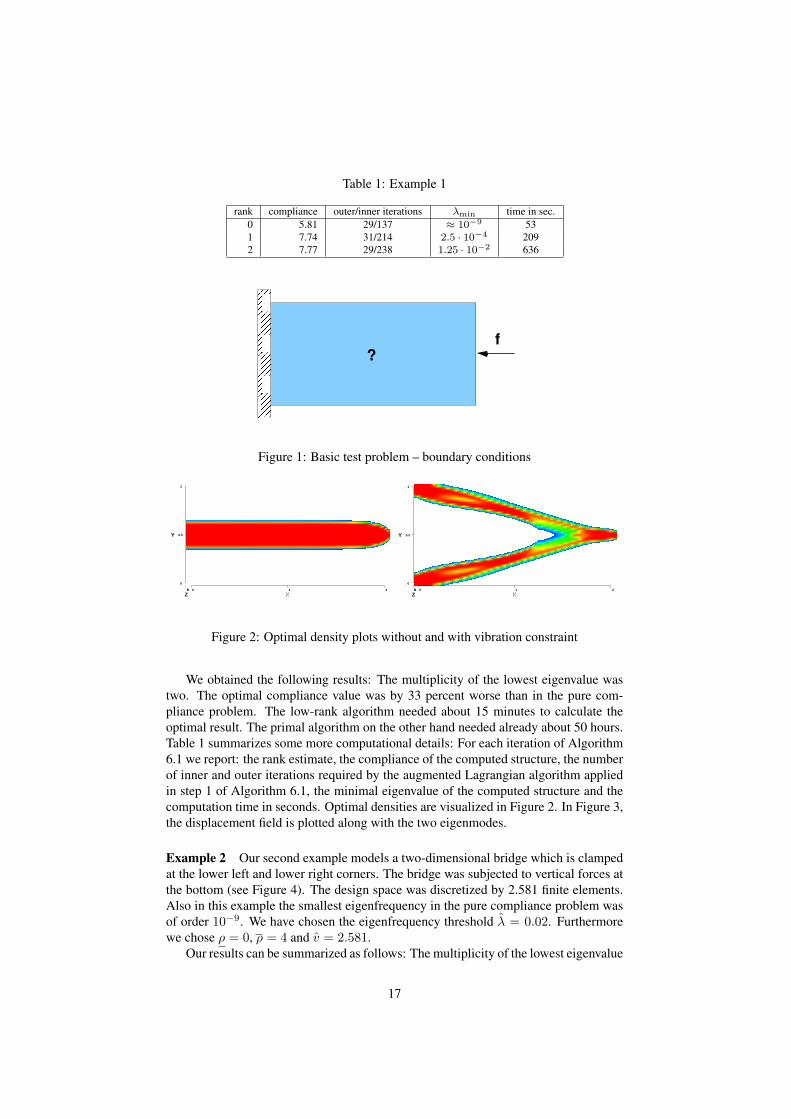
Table 1: Example 1

rank compliance outer/inner iterations λmin time in sec.0 5.81 29/137 ≈ 10−9 531 7.74 31/214 2.5 · 10−4 2092 7.77 29/238 1.25 · 10−2 636

f?

Figure 1: Basic test problem – boundary conditions

X 0 0 1 1 2 2

XZZ 0 0 0 0 0 0

YY

1 1

0.5 0.5

0 0

X 0 0 1 1 2 2

XZZ 0 0 0 0 0 0

YY

1 1

0.5 0.5

0 0

Figure 2: Optimal density plots without and with vibration constraint

We obtained the following results: The multiplicity of the lowest eigenvalue wastwo. The optimal compliance value was by 33 percent worse than in the pure com-pliance problem. The low-rank algorithm needed about 15 minutes to calculate theoptimal result. The primal algorithm on the other hand needed already about 50 hours.Table 1 summarizes some more computational details: For each iteration of Algorithm6.1 we report: the rank estimate, the compliance of the computed structure, the numberof inner and outer iterations required by the augmented Lagrangian algorithm appliedin step 1 of Algorithm 6.1, the minimal eigenvalue of the computed structure and thecomputation time in seconds. Optimal densities are visualized in Figure 2. In Figure 3,the displacement field is plotted along with the two eigenmodes.

Example 2 Our second example models a two-dimensional bridge which is clampedat the lower left and lower right corners. The bridge was subjected to vertical forces atthe bottom (see Figure 4). The design space was discretized by 2.581 finite elements.Also in this example the smallest eigenfrequency in the pure compliance problem wasof order 10−9. We have chosen the eigenfrequency threshold λ = 0.02. Furthermorewe chose ρ = 0, ρ = 4 and v = 2.581.

Our results can be summarized as follows: The multiplicity of the lowest eigenvalue

17

−0.5 0 0.5 1 1.5 2 2.5−0.2

0

0.2

0.4

0.6

0.8

1

1.2

X−axisY

−ax

is

−0.5 0 0.5 1 1.5 2 2.5−0.2

0

0.2

0.4

0.6

0.8

1

1.2

X−axis

Y−

axis

−0.5 0 0.5 1 1.5 2 2.5−0.2

0

0.2

0.4

0.6

0.8

1

1.2

X−axis

Y−

axis

Figure 3: Displacement field (top) and eigenmodes (bottom)

Table 2: Example 2

rank compliance inner/outer iterations λmin time in sec.0 168.29 13/68 ≈ 10−9 151 226.85 14/107 5.5 · 10−4 492 234.44 13/153 2.0 · 10−2 137

was again two. The optimal compliance value was by 25 percent worse than in the purecompliance problem. Computational details are provided in Table 2. Optimal densitiesare visualized in Figure 5. In Figure 6 we show the optimal displacement field alongwith the two eigenmodes corresponding to the lowest eigenfrequency.

Example 3 In our third example we considered a rectangular three-dimensional elas-tic body clamped on its left boundary and subjected to a load from the right (see Figure7). The design space was discretized by 3.200 finite elements. The optimal design cal-culated for the pure compliance problem resulted in a fundamental eigenvalue of order10−8. For the problem with eigenfrequency constraint we put λ = 0.16, ρ = 0, ρ = 2.5and v = 3.200.

This time we obtained the following results: The multiplicity of the lowest eigen-value is three. The optimal compliance value is only by 5 percent worse than for thepure compliance problem. The low-rank algorithm needed about 5 hours to calculatethe optimal result (compare Table 3 for details). Again we visualize optimal densi-ties (see Figure 8) and the corresponding displacement field along with the two mostsignificant eigenmodes of the optimal design (see Figure 9).

Remark 7.1. We calculated many more examples with different geometry, boundaryconditions and values of λ. In all these examples, the multiplicity of the smallesteigenvalue was never bigger than 8.

18

?

Figure 4: Basic test problem – boundary conditions

X 0 0 1.5 1.5 3 3

XZZ 0 0 0 0 0 0

YY

1 1

0.5 0.5

0 0

X 0 0 1.5 1.5 3 3

XZZ 0 0 0 0 0 0

YY

1 1

0.5 0.5

0 0

Figure 5: Optimal density plots without and with vibration constraint

−0.5 0 0.5 1 1.5 2 2.5 3 3.5

0

0.5

1

X−axis

Y−

axis

−0.5 0 0.5 1 1.5 2 2.5 3 3.5

0

0.5

1

X−axis

Y−

axis

−0.5 0 0.5 1 1.5 2 2.5 3 3.5

0

0.5

1

X−axis

Y−

axis

Figure 6: Displacement field (top) and eigenmodes (bottom)

Table 3: Example 3

rank compliance outer/inner iterations λmin time in sec.0 1.67 30/122 ≈ 10−8 4141 1.72 28/144 8.0 · 10−5 16702 1.73 29/181 1.0 · 10−2 58183 1.73 29/238 1.6 · 10−1 12776

19

?

Figure 7: Basic test problem – boundary conditions

X

0 0

5 5

10 10

XYY

5 5

2.5 2.5

0 0

ZZ 0 0

0.5 0.5

1 1

X

0 0

5 5

10 10

XYY

5 5

2.5 2.5

0 0

ZZ 0 0

0.5 0.5

1 1

Figure 8: Optimal density plots without and with vibration constraint

0

5

10

02

46

−0.50

0.51

1.5

X−axisY−axis

Z−

axis

0

5

10

02

46

−0.50

0.51

1.5

X−axisY−axis

Z−

axis

0

5

10

02

46

−0.50

0.51

1.5

X−axisY−axis

Z−

axis

Figure 9: Displacement field (top) and 2 eigenmodes (bottom)

20

A AppendixWe consider the following situation: Let V be a Hilbert space, equipped with the innerproduct (·, ·)V and the corresponding norm ‖ · ‖V . Let further a : V × V → R bea bounded, symmetric and V-elliptic bilinear form. An abstract eigenvalue problem isdefined as follows: Find λ ∈ R and u ∈ V , u 6= 0, such that

a(u, v) = λ(u, v)V ∀v ∈ V. (33)

The following theorem deals with the existence of solutions of the latter problem (see,for example, [12] or [21]):

Theorem A.1. There exists an increasing sequence of positive eigenvalues of problem(33) tending to∞:

0 < λ1 ≤ λ2 ≤ . . . , λk →∞ for k →∞

and an orthonormal basis wn of V consisting of the normalized eigenfunctions as-sociated with λn:

a(wn, v) = λn(wn, v) ∀v ∈ V, ‖wn‖V = 1.

Furthermore the following formula holds true for λ1:

λ1 = minv∈V,v 6=0

a(v, v)‖v‖2V

.

Now we want to apply Theorem A.1 to the generalized eigenvalue problem (10).The following obvious inclusion holds true for the bilinear forms in (9):

ker(bE) ⊂ ker(aE). (34)

Based on this observation, we define a Banach space V as the factor space V \ker(bE).On V × V we further define the inner product

(u, v)V := bE(u, v), (35)

where u, v are arbitrary representatives of the equivalence classes u and v, respectively.The inner product (·, ·)V induces the norm ‖u‖V :=

√bE(u, u) on V . Consequently,

V is a Hilbert space. Next we define the bilinear form

aE(u, v) := aE(u, v), (36)

where again u, v are arbitrary representatives of the equivalence classes u and v. Defin-ing the eigenvalue problem: Find λ ∈ R and u ∈ V , u 6= 0, such that

aE(u, v) = λ(u, v)V ∀v ∈ V, (37)

we are able to state the following corollary:

Corollary A.2. There exists an increasing sequence of well defined eigenvalues ofproblem (10) tending to∞:

0 ≤ λ1 ≤ λ2 ≤ . . . , λk →∞ for k →∞

21

and associated eigenfunctions wn, n = 1, 2, . . ., orthonormal w.r.t. the inner product(·, ·)V , such that

aE(wn, v) = λnbE(wn, v) ∀v ∈ V.

Furthermore the following formula holds true for λ1:

λ1 = minv∈V,v /∈ker(bE)

aE(v, v)bE(v, v)

= minv∈V,bE(v,v)=1

aE(v, v).

Proof. Suppose for a moment that aE is V-elliptic. Then we are able to apply TheoremA.1 to problem (37) and all assertions of Corollary A.2 follow immediately from (34),(35) and (36). On the other hand, if aE fails to be V-elliptic, we define a bilinear forma′E by

a′E(u, v) := a′E(u, v) + µ(u, v)V .

Obviously a′E is V-elliptic for any (arbitrary small) positive µ ∈ R. Applying TheoremA.1 to V and a′E we obtain the following estimates for the eigenvalues of problem (37)

−µ < λ1 ≤ λ2 ≤ . . . , λk →∞ for k →∞.

As µ can be chosen arbitrarily small we conclude that 0 ≤ λ1 and the proof is complete.

Let us finally define the bilinear form cE,λ(u, v) := aE(u, v) − λbE(u, v) andconsider the eigenvalue problem:

Find λ ∈ R, u ∈ V, u 6= 0 such that cE,λ(u, v) = λ(u, v) ∀v ∈ V. (38)

Then the following result proves the equivalence of (11) and (12).

Corollary A.3. The following assertions are equivalent:

a) The smallest well defined eigenvalue of the generalized eigenvalue problem (10)is nonnegative.

b) The smallest eigenvalue of the eigenvalue problem (38) is nonnegative.

Proof. Using Corollary A.2 and equation (34), we have

a) ⇔ aE(v, v)bE(v, v)

≥ λ ∀v ∈ V, v /∈ ker(bE)

⇔ aE(v, v)− λbE(v, v) ≥ 0 ∀v ∈ V, v /∈ ker(bE)(34)⇔ aE(v, v)− λbE(v, v) ≥ 0 ∀v ∈ V, v 6= 0

⇔ aE(v, v)− λbE(v, v)‖v‖2

≥ 0 ∀v ∈ V, v 6= 0

⇔ aE(v, v)− λbE(v, v) ≥ 0 ∀v ∈ V, ‖v‖ = 1 ⇔ b).

22

B AppendixIn the sequel we give a proof of Proposition 5.2:

Proof. We start with the KKT conditions of problem (24) in standard form: Let

F :=

(u, α,W, βl, βu) ∈ RN+1 × SN × R2M |W < 0, βl ≥ 0, βu ≥ 0

and x∗ := (u∗, α∗,W ∗, βl∗, βu

∗) ∈ F . Then a pair (x∗, E∗) is a KKT point of (24) if

and only if the conditions

gi(x∗) 4 0, E∗i < 0, i = 1, 2, . . . ,M, (39)

∇u,αf(x∗)−M∑i=1

〈E∗i ,∇u,αgi(x∗)〉 = 0, (40)

(W ∗, βl∗, βu

∗)> − ProjF

((W ∗, βl

∗, βu

∗)> −∇W,βl,βuf(x∗)

−M∑i=1

〈E∗i ,∇W,βl,βugi(x∗)〉)

= 0,(41)

〈E∗i , gi(x∗)〉 = 0, i = 1, 2, . . . ,M, (42)

with

f(u, α,W, βl, βu) = 2f>u− αV + ρ

M∑i=1

βli − ρM∑i=1

βui

are satisfied. Now we have

∂

∂uf(x∗) = 2f

∂

∂αf(x∗) = −V

∂

∂Wf(x∗) = 0

∂

∂βlif(x∗) = ρ, (i = 1, 2, . . . ,M)

∂

∂βuif(x∗) = −ρ, (i = 1, 2, . . . ,M)

∂

∂u

( M∑i=1

〈E∗i , gi(x∗)〉)

=M∑i=1

G∑j=1

∂

∂u〈E∗i , B>ijuu>Bij〉|u=u∗

=M∑i=1

G∑j=1

2BijE∗i B>iju∗

= 2A(E∗)u∗

23

∂

∂α

( M∑i=1

〈E∗i ,∇gi(x∗)〉)

=M∑i=1

〈E∗i ,−I〉 = −M∑i=1

Tr(E∗i )

∂

∂W

( M∑i=1

〈E∗i ,∇gi(x∗)〉)

=M∑i=1

〈E∗i ,∂

∂W(G∑j=1

B>ijWBij)− λ∗〈W,Mi〉I〉|W=W∗

=M∑i=1

G∑j=1

BijE∗i B>ij − λ∗Mi〈E∗i , I〉 = A(E∗)− λ∗M(E∗)

∂

∂βl( M∑i=1

〈E∗i ,∇gi(x∗)〉)

= 〈E∗i ,−I〉 = −Tr(E∗i )

∂

∂βu( M∑i=1

〈E∗i ,∇gi(x∗)〉)

= 〈E∗i , I〉 = Tr(E∗i ).

Hence (40) is equivalent to

A(E∗)u∗ = f,

M∑i=1

Tr(E∗i ) = V,

and (41) is equivalent to

ρ ≤ Tr(E∗i ) ≤ ρ (i = 1, 2, . . . ,M),

Sβl∗(ρ− Tr(E∗i )) = 0, βu

∗(Tr(E∗i )− ρ) = 0, (i = 1, 2, . . . ,M),

A(E∗)− λ∗M(E∗) < 0, 〈A(E∗)− λ∗M(E∗),W ∗〉 = 0.

Next, we see from (39) that (42) is equivalent to

M∑i=1

〈E∗i , gi(x∗)〉 = 0.

We further calculateM∑i=1

⟨E∗i , gi(x

∗)⟩

=M∑i=1

⟨E∗i ,

G∑j=1

B>ij(u∗u∗>+W ∗)Bij − (λ〈W ∗,Mi〉+ α∗ + βl

∗− βu

∗)I⟩

= −α∗M∑i=1

Tr(E∗i ) + u∗TA(E∗)u∗ + 〈W ∗, A(E∗)− λM(E∗)〉

+M∑i=1

βliTr(E∗i )−M∑i=1

βui Tr(E∗i )

= −α∗V + f>u∗ + ρ

M∑i=1

βl − ρM∑i=1

βu.

and the proof is complete.

24

References[1] W. Achtziger and M. Kocvara. Structural topology optimization with eigenval-

ues. Technical Report No. 315, Institute of Applied Mathematics, University ofDortmund, Germany, 2006.

[2] A. Ben-Tal, M. Kocvara, A. Nemirovski, and J. Zowe. Free material design viasemidefinite programming. The multi-load case with contact conditions. SIAM J.Optimization, 9:813–832, 1997.

[3] M. Bendsøe and O. Sigmund. Topology Optimization. Theory, Methods and Ap-plications. Springer-Verlag, Heidelberg, 2002.

[4] M. P. Bendsøe, J. M. Guades, R.B. Haber, P. Pedersen, and J. E. Taylor. Ananalytical model to predict optimal material properties in the context of optimalstructural design. J. Applied Mechanics, 61:930–937, 1994.

[5] F. J. Bonnans and A. Shapiro. Perturbation Analysis of Optimization Probelms.Springer-Verlag New-York, 2000.

[6] S. Burer and R.D.C. Monteiro. A nonlinear programming algorithm for solvingsemidefinite programs via low-rank factorization. Mathematical Programming(series B), 95(2):329–357, 2003.

[7] S. Burer and R.D.C. Monteiro. Local minima and convergence in low-ranksemidefinite programming. Mathematical Programming (series A), 103:427–444,2005.

[8] P. G. Ciarlet. The Finite Element Method for Elliptic Problems. North-Holland,Amsterdam, New York, Oxford, 1978.

[9] A. Diaz and N. Kikuchi. Solution to shape and topology eigenvalue optimizationproblems using a homogenization method. Int. J. Numer. Meth. Eng., 35:1487–1502, 1992.

[10] J. Du and N. Olhoff. Topological design of freely vibrating continuum structuresfor maximum values of simple and multiple eigenfrequencies and frequency gaps.Structural and Multidisciplinary Optimization, 34:91–110, 2007.

[11] I. Ekeland and Thomas Turnbull. Infinite-Dimensional Optimization and Convex-ity. University of Chicago Press, 1983.

[12] J. Haslinger and R. Makinen. Introduction to shape optimization. SIAM,Philadelphia, PA, 2002.

[13] M. Kocvara, M. Stingl, and J. Zowe. Free material optimization: recent progress.Optimization, 57:79–100, 2008.

[14] M. Kocvara, F. Leibfritz, M. Stingl, and D. Henrion. A nonlinear SDP algo-rithm for static output feedback problems in COMPlib. In Pavel Piztek, editor,Proceedings of the 16th IFAC World Congress. Elsevier, Amsterdam, 2005.

[15] M. Kocvara and M. Stingl. PENNON—a code for convex nonlinear and semidef-inite programming. Optimization Methods and Software, 18(3):317–333, 2003.

25

[16] M. Kocvara and M. Stingl. Solving nonconvex SDP problems of structural opti-mization with stability control. Optimization Methods and Software, 19(5):595–609, 2004.

[17] M. Kocvara and M. Stingl. Free material optimization: Towards the stress con-straints. Structural and Multidisciplinary Optimization, 33(4-5):323–335, 2007.

[18] M. Kocvara and J. Zowe. Free material optimization: An overview. In A.H.Siddiqi and M. Kocvara, editors, Trends in Industrial and Applied Mathematics,pages 181–215. Kluwer Academic Publishers, Dordrecht, 2002.

[19] H. D. Mittelmann. Several SDP codes on sparse and other SDP problems. De-partment of Mathematics and Statistics, Arizona State University, Tempe, AZ,September 14, 2003.

[20] T. Nakamura and M. Ohsaki. A natural generator of optimum topology of planetrusses for specified fundamental frequency. Computer Methods in Applied Me-chanics and Engineering, 94:113–129, 1992.

[21] J. Necas. Monographie Les Methodes directes en theorie des equations ellip-tiques. Masson et Cie, 1967.

[22] M. Ohsaki, K. Fujisawa, N. Katoh, and Y. Kanno. Semi-definite programmingfor topology optimization of truss under multiple eigenvalue constraints. Comp.Meths. Appl. Mech. Engrg., 1999. To appear.

[23] N. Olhoff. Optimal design with respect to structural eigenvalues. In F.P.J. Rim-rott and B. Tabarott, editors, Theoretical and Applied Mechanics, Proc. XVth Int.IUTAM Congress, pages 133–149. North-Holland, 1980.

[24] P. Pedersen. Maximization of eigenvalues using topology optimization. Structuraland Multidisciplinary Optimization, 20:2–11, 2000.

[25] J. Petersson and J. Haslinger. An approximation theory for optimum sheet inunilateral contact. Quarterly of Applied Mathematics, 56:309–325, 1998.

[26] R. T. Rockafellar. Convex Analysis. Princeton University Press, Princeton, NewJersey, 1970.

[27] M. Stingl. On the Solution of Nonlinear Semidefinite Programs by AugmentedLagrangian Methods. PhD thesis, Institute of Applied Mathematics II, Friedrich-Alexander University of Erlangen-Nuremberg, 2006.

[28] R. Werner. Free Material Optimization. PhD thesis, Institute of Applied Mathe-matics II, Friedrich-Alexander University of Erlangen-Nuremberg, 2000.

[29] H. Wolkowicz, R. Saigal, and L. Vandenberghe. Handbook on Semidefinite Pro-gramming. Kluwer, 2000.

[30] J. Zowe, M. Kocvara, and M. Bendsøe. Free material optimization via mathemat-ical programming. Math. Prog., Series B, 79:445–466, 1997.

26