free spa nning pipelines - rules and standards · and blevins (1994). ... line and cross -flow...
TRANSCRIPT

DET NORSKE VERITAS
RECOMMENDED PRACTICEDNV-RP-F105
FREE SPANNING PIPELINES
MARCH 2002
DNV-RP-F105.qxd 03-05-02 13:00 Page 2

Comments may be sent by e-mail to [email protected] subscription orders or information about subscription terms, please use [email protected] information about DNV services, research and publications can be found at http://www.dnv.com, or can be obtained from DNV, Veritasveien 1, N-1322 Høvik, Norway; Tel +47 67 57 99 00, Fax +47 67 57 99 11.
© Det Norske Veritas. All rights reserved. No part of this publication may be reproduced or transmitted in any form or by any means, including photocopying and recording, without the prior written consent of Det Norske Veritas.
Computer Typesetting (FM+SGML) by Det Norske Veritas.Printed in Norway
If any person suffers loss or damage which is proved to have been caused by any negligent act or omission of Det Norske Veritas, then Det Norske Veritas shall pay compensation to such personfor his proved direct loss or damage. However, the compensation shall not exceed an amount equal to ten times the fee charged for the service in question, provided that the maximum compen-sation shall never exceed USD 2 million.In this provision "Det Norske Veritas" shall mean the Foundation Det Norske Veritas as well as all its subsidiaries, directors, officers, employees, agents and any other acting on behalf of DetNorske Veritas.
FOREWORD
DET NORSKE VERITAS (DNV) is an autonomous and independent foundation with the objectives of safeguarding life, prop-erty and the environment, at sea and onshore. DNV undertakes classification, certification, and other verification and consultancyservices relating to quality of ships, offshore units and installations, and onshore industries worldwide, and carries out researchin relation to these functions.
DNV Offshore Codes consist of a three level hierarchy of documents:
— Offshore Service Specifications. Provide principles and procedures of DNV classification, certification, verification and con-sultancy services.
— Offshore Standards. Provide technical provisions and acceptance criteria for general use by the offshore industry as well asthe technical basis for DNV offshore services.
— Recommended Practices. Provide proven technology and sound engineering practice as well as guidance for the higher levelOffshore Service Specifications and Offshore Standards.
DNV Offshore Codes are offered within the following areas:
A) Qualification, Quality and Safety Methodology
B) Materials Technology
C) Structures
D) Systems
E) Special Facilities
F) Pipelines and Risers
G) Asset Operation
Amendments October 2003
This Code has been amended, but not reprinted in October 2003. The changes are incorporated in the printable (pdf) version.
All changes affecting DNV Offshore Codes that have not been reprinted, are published separately in the current Amendmentsand Corrections, issued as a printable (pdf) file.

Recommended Practice DNV-RP-F105, March 2002 Page 3
DET NORSKE VERITAS
CONTENTS
1 General ...................................................................................4 1.1 Introduction............................................................. 4 1.2 Objective .................................................................. 4 1.3 Scope and Application........................................... 4 1.4 Safety philosophy................................................... 5 1.5 Free Span Response Classification...................... 6 1.6 Flow regimes ........................................................... 6 1.7 Relationship to other Rules ................................... 7 1.8 Definitions ............................................................... 7 1.9 Abbreviations.......................................................... 7 1.10 Symbols .................................................................... 7
2 Design Criteria.................................................................. 10 2.1 General ................................................................... 10 2.2 Temporal classification ....................................... 10 2.3 Screening Fatigue Criteria .................................. 10 2.4 Fatigue Criterion................................................... 11 2.5 ULS Criterion........................................................ 12 2.6 Safety Factors........................................................ 13
3 Environmental Condi tions ............................................ 15 3.1 General ................................................................... 15 3.2 Current conditions................................................ 15 3.3 Short-term wave conditions................................ 16 3.4 Reduction functions............................................. 18 3.5 Long-term environmental modelling ................ 18 3.6 Return Period Values ........................................... 19
4 Response Models ...............................................................20 4.1 General....................................................................20 4.2 Marginal Fatigue Life Capacity..........................20 4.3 In-line Response Model.......................................21 4.4 Cross-flow Response Model...............................22
5 Force Model........................................................................25 5.1 General....................................................................25 5.2 FD solution for In-line direction.........................25 5.3 Simplified Fatigue Assessment...........................26 5.4 Force Coefficients .................................................26
6 Structural Analysis...........................................................29 6.1 General....................................................................29 6.2 Morphological classification...............................29 6.3 Structural modelling .............................................29 6.4 Functional Loads...................................................30 6.5 Static analysis ........................................................30 6.6 Eigen-value analysis .............................................31 6.7 Added Mass............................................................31 6.8 Approximate response quantities .......................31
7 Pipe -soil interaction..........................................................34 7.1 General....................................................................34 7.2 Modelling of pipe-soil interaction......................34 7.3 Approximate Soil Stiffness..................................35 7.4 Artificial supports..................................................38
8 References ...........................................................................39

Recommended Practice DNV-RP-F105, March 2002 Page 4
1 General
1.1 Introduction
1.1.1 The present document considers free spanning pipelines subjected to combined wave and current loading. The premises for the document are based on technical de-velopment within pipeline free span technology in recent R&D projects, as well as design experience from recent and ongoing projects, i.e. • DNV Guideline 14, see Mørk & Fyrileiv (1998) • The sections regarding Geotechnical Conditions and
part of the hydrodynamic model are based on the re-search performed in the GUDESP project, see Tura et al., (1994).
• The sections regarding Free Span Analysis and in-line Vortex Induced Vibrations (VIV) fatigue analyses are based on the published results from the MULTISPAN project, see Mørk et al., (1997).
• Numerical study based on CFD simulations for vibra-tions of a pipeline in the vicinity of a trench, per-formed by Statoil, DHI & DNV, see Hansen et al, 2001.
• Further, recent R&D and design experience e.g. from Åsgard Transport, ZEEPIPE, TOGI and TROLL OIL pipeline projects are implemented, see Fyrileiv & Mørk (1998).
The basic principles applied in this document are in agreement with most recognised rules and reflect state-of-the-art industry practice and latest research. This document includes a brief introduction of the basic hydrodynamic phenomena, principles and parameters. For a thorough introduction see e.g. Sumer & Fredsøe, (1997) and Blevins (1994).
1.2 Objective
1.2.1 The objective of this document is to provide ra-tional design criteria and guidance for assessment of pipe-line free spans subjected to combined wave and current loading.
1.3 Scope and Application
1.3.1 Detailed design criteria are specified for Ultimate Limit State (ULS) and Fatigue Limit State (FLS) due to in-line and cross-flow Vortex Induced Vibrations (VIV) and direct wave loading. The following topics are considered: • methodologies for free span analysis; • requirements for structural modelling; • geotechnical conditions ; • environmental conditions & loads; • requirements for fatigue analysis; • response and direct wave force analysis models; and
• acceptance criteria.
1.3.2 Free spans can be caused by: • seabed unevenness • change of seabed topology (e.g. scouring, sand waves) • artificial supports/rock berms etc.
1.3.3 The following environmental flow conditions are described in this document: • steady flow due to current; • oscillatory flow due to waves; and • combined flow due to current and waves. The flow regimes are discussed in section 1.6.
1.3.4 There are no limitations to span length and span gap with respect to application of this Recommended Prac-tice. The basic cross-flow VIV Response model is, however, based on single mode response.
In case several potential vibration modes can become ac-tive at a given flow velocity, the mode associated with the largest contribution to the fatigue damage shall be applied. Unless otherwise documented the damage contribution for any modes should relate to the same critical (weld) loca-tion.
1.3.5 The free span analysis may be based on approxi-mate response expressions or a refined FE approach de-pending on the free span classification, see section 6.2. The following cases are considered: • single spans • spans interacting with adjacent/side spans. The stress ranges and natural frequencies should normally be obtained from an FE-approach. Requirements to the structural modelling and free span analyses are given in section 6.
1.3.6 The following models are considered: • Response Models (RM) • Force Models (FM) An amplitude response model is applicable when the vibration of the free span is dominated by vortex induced resonance phenomena. A force model may be used when the free span response can be found through application of calibrated hydrodynamic loads. The selection of an appropriate model may be based on the prevailing flow regimes, see section 1.6.
1.3.7 The fatigue criterion is limited to stress cycles within the elastic range. Low cycle fatigue due to elasto-plastic behaviour is considered outside the scope of this document.
Recommended Practice DNV-RP-F105, March 2002 Page 5
DET NORSKE VERITAS
1.3.8 Fatigue loads due to trawl interaction, cyclic loads during installation or pressure variations are not con-sidered herein but must be considered as a part of the inte-grated fatigue damage assessment.
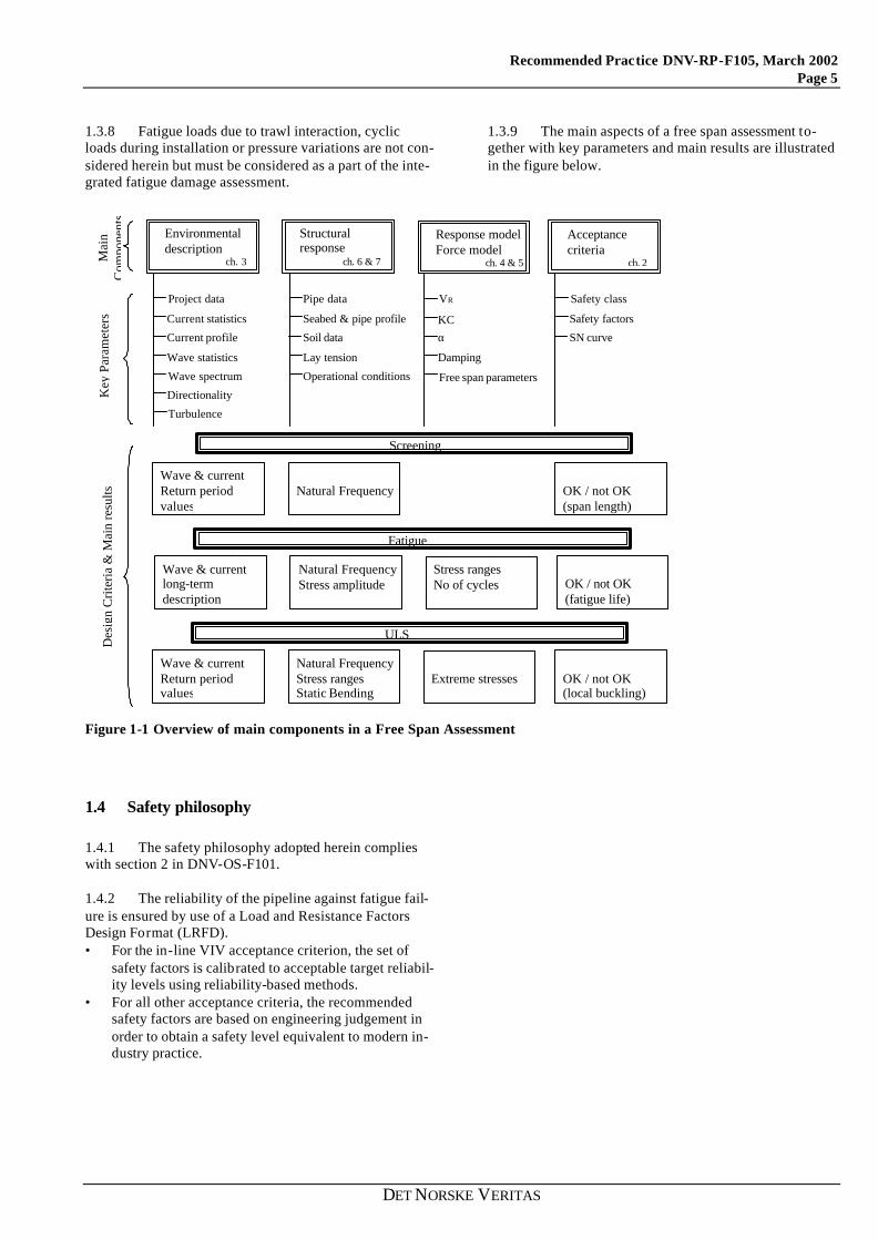
1.3.9 The main aspects of a free span assessment to-gether with key parameters and main results are illustrated in the figure below.
Environmentaldescription
ch. 3
Project data
Current statistics
Current profile
Wave statistics
Wave spectrum
Directionality
Turbulence
Wave & currentReturn periodvalues
Wave & currentlong-termdescription
Screening
Fatigue
ULS
Wave & currentReturn periodvalues
Structuralresponse
ch. 6 & 7
Pipe data
Seabed & pipe profile
Soil data
Lay tension
Operational conditions
Natural Frequency
Natural FrequencyStress amplitude
Natural FrequencyStress rangesStatic Bending
Response modelForce model
ch. 4 & 5
VR
KCα
Damping
Free span parameters
Stress rangesNo of cycles
Extreme stresses
Acceptancecriteria
ch. 2
Safety class
Safety factors
SN curve
OK / not OK(span length)
OK / not OK(fatigue life)
OK / not OK(local buckling)
Mai
nC
ompo
nent
sK
ey P
aram
eter
sD
esig
n C
rite
ria
& M
ain
resu
lts
Figure 1-1 Overview of main components in a Free Span Assessment
1.4 Safety philosophy
1.4.1 The safety philosophy adopted herein complies with section 2 in DNV-OS-F101.
1.4.2 The reliability of the pipeline against fatigue fail-ure is ensured by use of a Load and Resistance Factors Design Format (LRFD). • For the in-line VIV acceptance criterion, the set of
safety factors is calibrated to acceptable target reliabil-ity levels using reliability-based methods.
• For all other acceptance criteria, the recommended safety factors are based on engineering judgement in order to obtain a safety level equivalent to modern in-dustry practice.

Recommended Practice DNV-RP-F105, March 2002 Page 6
1.5 Free Span Response Classification
1.5.1 An overview of typical free span characteristics is given in the table below as a function of the free span
length. The ranges indicated for the normalised free span length in terms of (L/D) are tentative and given for illus-tration only.
L/D Response description
L/D<30 1) Very little dynamic amplification. Normally not required to perform comprehensive fatigue design check. Insignificant dynamic re -sponse from environmental loads expected and unlikely to experience VIV.
30<L/D<100 Response dominated by beam behaviour Typical span length for operating conditions. Natural frequencies sensitive to boundary conditions (and effective axial force).
100<L/D<200 Response dominated by combined beam and cable behaviour Relevant for free spans at uneven seabed in temporary conditions. Natural frequencies sensitive to boundary conditions, effective axial force (including initial deflection, geometric stiffness) and pipe “feed in”.
L/D>200 Response dominated by cable behaviour Relevant for small diameter pipes in temporary conditions. Natural frequencies governed by de-flected shape and effective axial force.
1) For hot pipelines (response dominated by the effective axial force) or under extreme current conditions (Uc > 1.0-2.0 m/s) this L/D limit may be misleading.
1.6 Flow regimes
1.6.1 The current flow velocity ratio, α=Uc/(Uc+Uw) (where Uc is the current velocity normal to the pipe and Uw
is the significant wave induced velocity amplitude normal to the pipe, see section 4) may be applied to classify the flow regimes as follows:
α < 0.5 wave dominant - wave superimposed by current.
In-line direction: in-line loads may be described according to Morison’s formulae, see section 5. In-line VIV due to vortex shedding is negligible. Cross-flow direction: cross-flow loads are mainly due to asymmetric vortex shedding. A response model, see section 4, is recommended.
0.5< α < 0.8 wave dominant – current superimposed by wave In-line direction: in-line loads may be described according to Morison’s formulae, see section 5. In-line VIV due to vortex shedding is mitigated due to the presence of waves. Cross-flow direction: cross-flow loads are mainly due to asymmetric vortex shedding and resemble the current dominated situation. A response model, see section 4, is recommended.
α > 0.8 current dominant In-line direction: in-line loads comprises the following components : • a steady drag dominated comp onent • a oscillatory component due to regular vortex shedding For fatigue analyses a response model applies, see section 4. In -line loads according to Morison’s formulae are normally negligible. Cross-flow direction: cross-flow loads are cyclic and due to vortex shedding and resembles the pure current situation. A response model, see section 4, is recommended.
Note that α=0 correspond to pure oscillatory flow due to waves and α =1 corresponds to pure (steady) current flow. The flow regimes are illustrated in Figure 1-2.

Recommended Practice DNV-RP-F105, March 2002 Page 7
DET NORSKE VERITAS
-2
-1
0
1
2
3
4
5
6
time
Flo
w V
eloc
ity(
Uc+
Uw)
current dominated flow
wave dominated flow α=0.8
α=0.0
α=0.5
Figure 1-2 Flow regimes
1.6.2 Oscillatory flow due to waves is stochastic in nature, and a random sequence of wave heights and asso-ciated wave periods generates a random sequence of near seabed horizontal oscillations. For VIV analyses, the sig-nificant velocity amplitude, Uw, is assumed to represent a single sea-state. This is likely to be a conservative ap-proximation.
1.7 Relationship to other Rules
1.7.1 This document formally supports and complies with the DNV Offshore Standard “Submarine Pipeline Systems”, DNV-OS-F101, 2000 and is considered to be a supplement to relevant National Rules and Regulations.
1.7.2 This document is supported by other DNV off-shore codes as follows: • Recommended Practice DNV-RP-C203 “Fatigue
Strength Analysis of Offshore Steel Structures” • Offshore Standard DNV-OS-F201 “Dynamic Risers” • Classification Note No. 30.5 “Environmental Condi-
tions and Environmental Loads”, 2000. In case of discrepancies between the recommendations, this Document supersedes the Recommended Practice and Classification Notes listed above.
1.8 Definitions
1.8.1 Effective Span Length is the length of an idealised fixed-fixed span having the same structural response in terms of natural frequencies as the real free span supported on soil.
1.8.2 Force Model is in this document a model where the environmental load is based on Morison’s force ex-pression.
1.8.3 Gap is defined as the distance between the pipe and the seabed. The gap used in design, as a single repre-sentative value, must be characteristic for the free span The gap may be calculated as the average value over the central third of the span.
1.8.4 Marginal Fatigue Capacity is defined as the fa-tigue capacity (life) with respect to one seastate defined by its significant wave height, peak period and direction.
1.8.5 Response Model is a model where the structural response due to VIV is determined by hydrodynamical parameters.
1.8.6 Span Length is defined as the length where a con-tinuous gap exists, i.e. as the visual span length.
1.9 Abbreviations CSF concrete stiffness factor FM force model LRFD load and resistance factors des ign format OCR over-consolidation ratio (only clays) RM response model (VIV) RD response domain RPV return period values TD time domain ULS ulitmate limit state VIV vortex induced vibrations
1.10 Symbols
1.10.1 Latin aκ parameter for rain-flow counting factor
a characteristic fatigue strength constant
Ae external cross-section area Ai internal cross-section (bore) area AIL inline unit amplitude stress (stress induced by
a pipe (vibration mode) deflection equal to an outer diameter D)
ACF cross-flow unit amplitude stress As pipe steel cross section area (AY/D) normalised in-line VIV amplitude (AZ/D) normalised cross-flow VIV amplitude B chord corresponding to pipe embedment
equal to v or linearisation constant bκ parameter for rainflow counting factor Ca added mass coefficient (CM-1) CD drag coefficient CM the inertia coefficient CL coefficient for lateral soil stiffness CV coefficient for vertical soil stiffness CT constant for long-term wave period distribu-
tion C1-6 Boundary condition coefficients c(s) soil damping per unit length D pipe outer diameter (including any coating) Dfat deterministic fatigue damage Ds outer steel diameter E Young's modulus EI bending stiffness E seabed gap es void ratio

Recommended Practice DNV-RP-F105, March 2002 Page 8
(e/D) seabed gap ratio f0 in-line (f0,in) or cross-flow (f0,cr) natural fre -
quency (determined at no flow around the pipe)
fsn concrete construction strength fs vortex shedding frequency (Strouhal
frequency) =DU
St
FL lateral pipe-soil contact force FV vertical pipe-soil contact force fv dominating vibration frequency fw wave frequency F() distribution function g gravity gc correction function due to steady current gD drag force term gI inertia force term G shear modulus of soil or incomplete comple-
mentary Gamma function G(ω) frequency transfer function from wave eleva-
tion to flow velocity Heff effective lay tension HS significant wave height h water depth, i.e. distance from the mean sea
level to the pipe I moment of inertia Ic turbulence intensity over 30 minutes ip plasticity index, cohesive soils k Wave number kc soil parameter or empirical constant for con-
crete stiffening kp peak factor ks soil coefficient kw normalisation constant K soil stiffness KL lateral (horizontal) dynamic soil stiffness KV vertical dynamic soil stiffness (k/D) pipe roughness KC Keulegan Carpenter number =
DfU
w
w
KS stability parameter =
2Te
D
m4
ρ
ζπ
K0 coefficient of earth pressure at rest k1 soil stiffness k2 soil stiffness L free span length, (apparent, visual) La length of adjacent span Leff effective span length Ls span length with vortex shedding loads Lsh length of span shoulder me effective mass per unit length m fatigue exponent m(s) mass per unit length including structural
mass, added mass and mass of internal fluid Mn spectral moments of order n ni number of stress cycles for stress block i N number of independent events in a return
period Ni number of cycles to failure for stress block i
Ntr true steel wall axial force Nc soil bearing capacity parameter Nq soil bearing capacity parameter Nγ soil bearing capacity parameter pe external pressure pi internal pressure Pi probability of occurrence for i’th stress cycle q deflection load per unit length PE Euler load = (1+CSF)π2 EI/Leff
2 Ra axial soil reaction Rc current reduction factor RD reduction factor from wave direction and
spreading Rv vertical soil reaction RIθ reduction factor from turbulence and flow
direction Rk reduction factor from damping
Re Reynolds number D= ν
UD
s spreading parameter S stress range, i.e. double stress amplitude Ssw stress at intersection between two SN-curves Seff effective axial force Sηη wave spectral density SSS stress spectra SUU wave velocity spectra at pipe level su undrained shear strength, cohesive soils St Strouhal number t pipe wall thickness or time Texposure load exposure time Tlife fatigue design life capacity Tp peak period Tu mean zero up-crossing period of oscillating
flow Tw wave period U current velocity Uc current velocity normal to the pipe Us significant wave velocity Uw significant wave induced flow velocity normal
to the pipe, corrected for wave direction and spreading
v vertical soil settlement (pipe embedment)
VR reduced velocity =DfUU
0
wc +
w wave energy spreading function y lateral pipe displacement z height above seabed or in-line pipe displace-
ment zD height to the mid pipe zm macro roughness parameter z0 sea-bottom roughness zr reference (measurement) height

Recommended Practice DNV-RP-F105, March 2002 Page 9
DET NORSKE VERITAS
1.10.2 Greek α current flow velocity ratio, generalised Phil-
lips’ constant or Weibull scale parameter αe temperature expansion coefficient β Weibull shape parameter and relative soil
stiffness parameter ∆/D relative trench depth ∆pi internal pressure difference relative to laying ∆T temperature difference relative to laying or
storm duration δ pipe deflection ε band-width parameter Γ gamma function γ peak-enhancement factor for JONSWAP
spectrum or Weibull location parameter γsoil total unit weight of soil γsoil’ submerged unit weight of soil γwater unit weight of water γs safety factor on stress amplitude γf safety factor on natural frequency γcr safety factor for cross-flow screening criterion γin safety factor for in-line screening criterion γk safety factor on stability parameter γon safety factor on onset value for VR
κRFC rainflow counting factor κ curvature λ1 mode shape factor λmax equivalent stress factor η usage factor µ mean value µa axial friction coefficient µL lateral friction coefficient ν Poisson's ratio
or kinematic viscosity (≈1.5·10-6 [m2/s] φ mode shape Φ() cumulative normal distribution function ϕ() normal distribution function ϕs angle of friction, cohesionless soils ψk,CM correction factor for CM due to pipe rough-
ness ψtrench,CM correction factor for CM due to effect of pipe
in trench ψproxi,CM reduction factor for CM due to seabed prox-
imity ψk,CD correction factor for CD due to pipe rough-
ness ψtrench,CD correction factor for CD due to effect of pipe
in trench ψA,CD amplification factor for CD due to cross-flow
vibrations ψproxi,CD reduction factor for CD due to seabed prox-
imity ψproxi,onset correction factor for onset cross-flow due to
seabed proximity ψmass,onset correction factor for onset cross-flow due to
specific mass of the pipe ψα,onset correction factor for onset cross-flow due to
waves
ψtrench,onset reduction factor for onset cross-flow due to the effect of a trench
ψα,in correction factor for onset cross-flow due to seabed proximity
ρ density of water ρs/ρ specific mass ratio between the pipe mass (not
including added mass) and the displaced wa-ter.
σ stress, spectral width parameter or standard deviation
σc standard deviation of current velocity fluctua-tions
σu standard deviation of wave induced flow ve-locity
σdyn dynamic stress σl longitudinal stress σN static axial stress σstat static stress σs effective soil stress or standard deviation of
wave induced stress amplitude θrel relative angle between flow and pipeline di-
rection ̄θ flow direction ζΤ total modal damping ratio ζsoil soil modal damping ratio ζstr structural modal damping ratio ζh hydrodynamic modal damping ratio ω0 angular natural frequency ω angular wave frequency ωp angular spectral peak wave frequency τmax soil shear strength
1.10.3 Subscripts IL in-line CF cross-flow onset onset of VIV 100year 100 year return period value 1year 1 year return period value
Recommended Practice DNV-RP-F105, March 2002 Page 10
2 Design Criteria
2.1 General
2.1.1 For all temporary and permanent free spans a free span assessment addressing the integrity with respect to fatigue and local buckling (ULS) shall be performed.
2.1.2 Vibrations due to vortex shedding and direct wave loads are acceptable provided the fatigue and ULS criteria specified herein is fulfilled.
2.1.3 In case several potential vibration mo des can be-come active at a given flow velocity, the mode associated with the largest contribution to the fatigue damage shall be applied. Unless otherwise documented the damage contri-bution for any modes should relate to the same critical (weld) location.
2.1.4 The following functional requirements apply: • The aim of fatigue design is to ensure an adequate
safety against fatigue failure within the design life of the pipeline.
• The fatigue analysis should cover a period which is representative for the free span exp osure period.
• All stress fluctuations imposed during the entire de-sign life of the pipeline capable of causing fatigue damage shall be accounted for.
• The local fatigue design checks are to be performed at all free spanning pipe sections accounting for damage contributions from all potential vibration modes re-lated to the actual and neighbouring spans.
Start
Free Span Data &Characteristics
OK
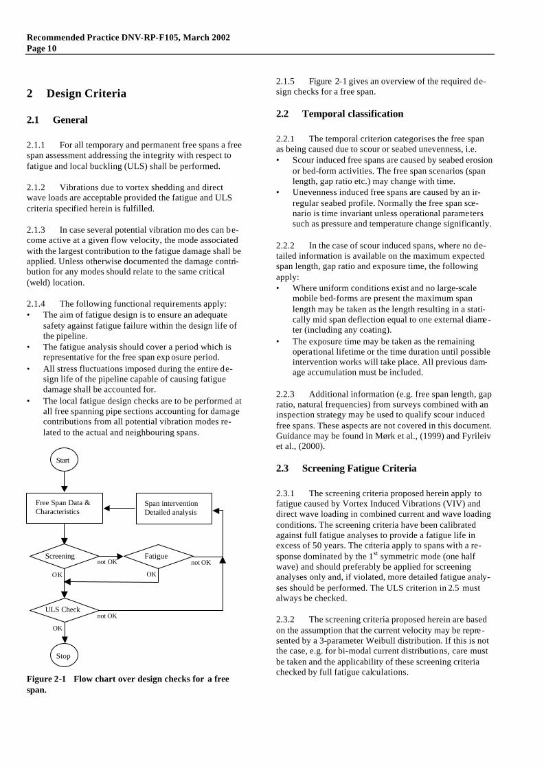
Screening Fatigue
ULS Check
Stop
Span interventionDetailed analysis
not OK
not OK
OK
OK
not OK
Figure 2-1 Flow chart over design checks for a free span.
2.1.5 Figure 2-1 gives an overview of the required de-sign checks for a free span.
2.2 Temporal classification
2.2.1 The temporal criterion categorises the free span as being caused due to scour or seabed unevenness, i.e. • Scour induced free spans are caused by seabed erosion
or bed-form activities. The free span scenarios (span length, gap ratio etc.) may change with time.
• Unevenness induced free spans are caused by an ir-regular seabed profile. Normally the free span sce-nario is time invariant unless operational parameters such as pressure and temperature change significantly.
2.2.2 In the case of scour induced spans, where no de-tailed information is available on the maximum expected span length, gap ratio and exposure time, the following apply: • Where uniform conditions exist and no large-scale
mobile bed-forms are present the maximum span length may be taken as the length resulting in a stati-cally mid span deflection equal to one external diame-ter (including any coating).
• The exposure time may be taken as the remaining operational lifetime or the time duration until possible intervention works will take place. All previous dam-age accumulation must be included.
2.2.3 Additional information (e.g. free span length, gap ratio, natural frequencies) from surveys combined with an inspection strategy may be used to qualify scour induced free spans. These aspects are not covered in this document. Guidance may be found in Mørk et al., (1999) and Fyrileiv et al., (2000).
2.3 Screening Fatigue Criteria
2.3.1 The screening criteria proposed herein apply to fatigue caused by Vortex Induced Vibrations (VIV) and direct wave loading in combined current and wave loading conditions. The screening criteria have been calibrated against full fatigue analyses to provide a fatigue life in excess of 50 years. The criteria apply to spans with a re-sponse dominated by the 1st symmetric mode (one half wave) and should preferably be applied for screening analyses only and, if violated, more detailed fatigue analy-ses should be performed. The ULS criterion in 2.5 must always be checked.
2.3.2 The screening criteria proposed herein are based on the assumption that the current velocity may be repre-sented by a 3-parameter Weibull distribution. If this is not the case, e.g. for bi-modal current distributions, care must be taken and the applicability of these screening criteria checked by full fatigue calculations.

Recommended Practice DNV-RP-F105, March 2002 Page 11
DET NORSKE VERITAS
2.3.3 The in-line natural frequency f0,IL must fulfil:
αγ⋅
−⋅
⋅>
γIL
ILonset,R
year100,c
f
IL,0
250D/L1
DV
Uf
Where
γf Safety factor on the natural frequency, see 2.6
γIL Screening factor for inline, see 2.6
α
Current flow ratio=
+6.0;
UU
Umax
year100,cyear1,w
year100,c
D Outer pipe diameter incl. coating L Free span length Uc,100year 100 year return period value for the cur-
rent velocity at the pipe level, see 3 Uw,1year Significant 1 year return period value for
the wave induced flow velocity at the pipe level corresponding to the annual signifi-cant wave height Hs,1year, see 3
ILonset,RV In-line onset value for the reduced veloc-
ity, see 4.
If the above criterion is violated, then a full in-line VIV fatigue analysis is required.
2.3.4 The cross-flow natural frequency f0,CF must fulfil:
CFCFonset,R
year1,wyear100,c
f
CF,0
DV
UUfγ⋅
⋅
+>
γ
Where
γCF Screening factor for cross-flow, see 2.6 CF
onset,RV Cross-flow onset value for the reduced velocity, see 4
If the above criterion is violated, then a full in-line and cross-flow VIV fatigue analysis is required.
2.3.5 Fatigue analysis due to direct wave action is not required provided:
32
UU
U
year100,cyear1,w
year100,c >+
and the above screening criteria for in-line VIV is ful-filled. If this criterion is violated, then a full fatigue analy-ses due to in-line VIV and direct wave action is required
2.4 Fatigue Criterion
2.4.1 The fatigue criterion can be formulated as:
η⋅ Tlife ≥ Texposure
where η is the allowable fatigue damage ratio, Tlife the fatigue design life capacity and Texposure the life or load exposure time.
2.4.2 The fatigue damage assessment is based on the accumulation law by Palmgren-Miner:
∑=i
ifat N
nD
Where
Dfat Accumulated fatigue damage. ni Total number of stress cycles corresponding to the
(mid-wall) stress range Si N Number of cycles to failure at stress range Si Σ Implies summation over all stress fluctuations
in the design life
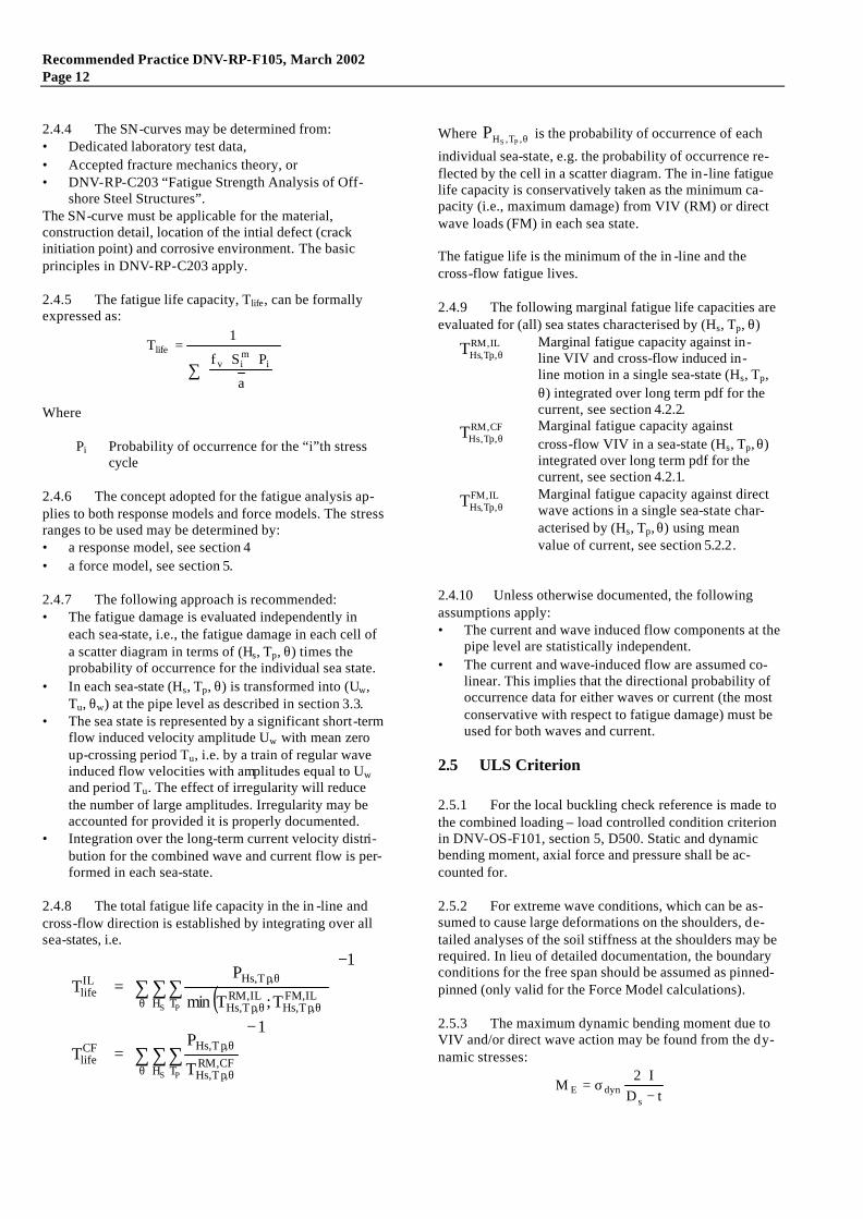
2.4.3 The number of cycles to failure at stress range S is defined by the SN curve of the form:
≤⋅
>⋅= −
−
swm
swm
SSSa
SSSaN
22
11
Where
m1, m2 Fatigue exponents (the inverse slope of the bi-linear S-N curve)
21 a,a Characteristic fatigue strength constant de-fined as the mean-minus-two-standard-deviation curve
Ssw Stress at intersection of the two SN-curves given by:
−
= 1
sw1
mNlogalog
sw 10S
Where Nsw is the number of cycles for which change in slope appear. LogNsw is typically 6 – 7.
1
10
100
1000
1.E+03 1.E+04 1.E+05 1.E+06 1.E+07 1.E+08 1.E+09 1.E+10
No of cycles, N
Str
ess
Ran
ge, S
NSW
SSW
(a1;m1)
(a2;m2 )
Figure 2-2 Typical two-slope SN curve.
Recommended Practice DNV-RP-F105, March 2002 Page 12
2.4.4 The SN-curves may be determined from: • Dedicated laboratory test data, • Accepted fracture mechanics theory, or • DNV-RP-C203 “Fatigue Strength Analysis of Off-
shore Steel Structures”. The SN-curve must be applicable for the material, construction detail, location of the intial defect (crack initiation point) and corrosive environment. The basic principles in DNV-RP-C203 apply.
2.4.5 The fatigue life capacity, Tlife, can be formally expressed as:
∑
⋅⋅=
a
PSf
1T
imiv
life
Where
Pi Probability of occurrence for the “i”th stress cycle
2.4.6 The concept adopted for the fatigue analysis ap-plies to both response models and force models. The stress ranges to be used may be determined by: • a response model, see section 4 • a force model, see section 5.
2.4.7 The following approach is recommended: • The fatigue damage is evaluated independently in
each sea-state, i.e., the fatigue damage in each cell of a scatter diagram in terms of (Hs, Tp, θ) times the probability of occurrence for the individual sea state.
• In each sea-state (Hs, Tp, θ) is transformed into (Uw, Tu, θw) at the pipe level as described in section 3.3.
• The sea state is represented by a significant short-term flow induced velocity amplitude Uw with mean zero up-crossing period Tu, i.e. by a train of regular wave induced flow velocities with amplitudes equal to Uw and period Tu. The effect of irregularity will reduce the number of large amplitudes. Irregularity may be accounted for provided it is properly documented.
• Integration over the long-term current velocity distri-bution for the combined wave and current flow is per-formed in each sea-state.
2.4.8 The total fatigue life capacity in the in -line and cross-flow direction is established by integrating over all sea-states, i.e.
( )1
T
PT
1
T;Tmin
PT
S P
S P
H TCF,RM,T p,Hs
,T p,HsCFlife
H TIL,FM
,T p,HsIL,RM,T p,Hs
,T p,HsILlife
−
=
−
=
∑ ∑∑
∑ ∑∑
θ θ
θ
θ θθ
θ
Where θ,T,H PSP is the probability of occurrence of each
individual sea-state, e.g. the probability of occurrence re-flected by the cell in a scatter diagram. The in-line fatigue life capacity is conservatively taken as the minimum ca-pacity (i.e., maximum damage) from VIV (RM) or direct wave loads (FM) in each sea state. The fatigue life is the minimum of the in -line and the cross-flow fatigue lives.
2.4.9 The following marginal fatigue life capacities are evaluated for (all) sea states characterised by (Hs, Tp, θ)
IL,RM,Tp,HsT θ
Marginal fatigue capacity against in-line VIV and cross-flow induced in-line motion in a single sea-state (Hs, Tp, θ) integrated over long term pdf for the current, see section 4.2.2.
CF,RM,Tp,HsT θ
Marginal fatigue capacity against cross-flow VIV in a sea-state (Hs, Tp, θ) integrated over long term pdf for the current, see section 4.2.1.
IL,FM,Tp,HsT θ
Marginal fatigue capacity against direct wave actions in a single sea-state char-acterised by (Hs, Tp, θ) using mean value of current, see section 5.2.2.
2.4.10 Unless otherwise documented, the following assumptions apply: • The current and wave induced flow components at the
pipe level are statistically independent. • The current and wave-induced flow are assumed co-
linear. This implies that the directional probability of occurrence data for either waves or current (the most conservative with respect to fatigue damage) must be used for both waves and current.
2.5 ULS Criterion
2.5.1 For the local buckling check reference is made to the combined loading – load controlled condition criterion in DNV-OS-F101, section 5, D500. Static and dynamic bending moment, axial force and pressure shall be ac-counted for.
2.5.2 For extreme wave conditions, which can be as-sumed to cause large deformations on the shoulders, de-tailed analyses of the soil stiffness at the shoulders may be required. In lieu of detailed documentation, the boundary conditions for the free span should be assumed as pinned-pinned (only valid for the Force Model calculations).
2.5.3 The maximum dynamic bending moment due to VIV and/or direct wave action may be found from the dy-namic stresses:
tDI2
Ms
dynE −⋅
σ=
Recommended Practice DNV-RP-F105, March 2002 Page 13
DET NORSKE VERITAS
Where
σdyn Dynamic stress given below I Moment of inertia
Ds Outer diameter of steel pipe t Wall thickness
2.5.4 The dynamic stress, σdyn, is taken as:
CFdyn
max,FMCF
ILCFILdyn
S21flowcross
S;AA
S5.0;Smax21
linein
=σ−
⋅=σ−
Where
SIL In-line stress range, see section 4 SCF Cross-flow stress range, see section 4
SFM,max Maximum stress range due to direct wave loading (force model) , see section 5
AIL In-line unit deflection stress amplitude due to VIV, see section 6.8.4
ACF Cross-flow unit deflection stress amplitude due to VIV, see section 6.8.4
The unit deflection stress amplitude A IL and ACF may be evaluated using the following return period environmental flow conditions:
( )( )year100,wyear10,cyear10,wyear100,cyear100
year10,wyear1,cyear1,wyear10,cyear10
year1,wyear1,cyear1
UU;UUmaxU
UU;UUmaxUUUU
++=
++=+=
2.5.5 For the cross-flow direction, the stress simply stems from the VIV induced amplitude. For the in -line direction, the dynamic stress range is taken as the maxi-mum of: • The return period stress range, e.g. 100 year, for in-
line VIV, Sin, defined in section 4.3. • The stress from 50% of the cross-flow induced VIV
motion. All parameters are defined in section 4.4.
2.5.6 The maximum dynamic stress σFM,max from direct wave loading may be calculated using a “design storm” approach using:
σFM,max= kp σs
where kp is the peak factor given by:
( )( )Tfln2
577.0Tfln2k
vvp
∆+∆=
∆T is the storm duration equal to 3 hour and fv is given in section 5.2. kp may conservatively be taken equal to 4.
σs is the standard deviation of the stress (amplitude) re -sponse calculated from a time domain or frequency do-main analysis, see section 5.
Alternatively a regular wave approach using Hmax may be applied.
2.5.7 A simplified ULS screening may be performed in terms of an equivalent stress check, ref. DNV-OS-F101, section 12, F1200.
2.5.8 The longitudinal stress is given by:
{ }dynstaticNl σ+σ±σ=σ
Where
σN Static axial stress from true wall axia l force, Ntr given by: σN = Ntr/As
σstatic Static bending stress from static bending mo-ment, see 6.8.6. Applies to both vertical and lateral directions.
σdyn Dynamic bending stress, see 2.5.4. Applies to both directions, in-line and cross-flow inde-pendently.
2.6 Safety Factors
2.6.1 The safety factors to be used with the screening criteria are listed below.
Table 2-1 Safety factors for screening criteria γIL 1.15 γCF 1.3
2.6.2 Pipeline reliability against fatigue uses the safety class concept, which takes account of the failure conse-quences, see DNV-OS-F101, Section 2. The following safety factor format is used:
( )η≤
•γγγγ⋅= ∑
a
)(P.),,(SfTD
monkfsv
osureexpfat
γf, γon, γk and γs denote partial safety factors for the natural frequency, onset of VIV, stability parameter and stress range respectively. The set of partial safety factor to be applied are specified in the table below for the individual safety classes.
Table 2-2 Safety factors for fatigue Safety Class Safety Factor
Low Normal High η 1.0 0.5 0.25 γs 1.051) (1.0)
γf 1.201) (1.15) γk 1.30 γon 1.10
1) This safety factor is intended to be used in design when detailed data about span length, gap etc is not known. If a span is assessed in-service with updated and measured span data, the safety factor in brackets may be used.

Recommended Practice DNV-RP-F105, March 2002 Page 14
Comments:
• η apply to both Response Model and Force Model • γs is to be multiplied to the stress (S γS) • γf applies to the natural frequency (fo/γf) • γon applies to onset values for in-line and cross-flow
VIV (VR,on/γon) • γk applies to the stability parameter (KS/γk) • For ULS, the calculation of load effects is to be per-
formed without safety factors (γS = γf = γk = γon = 1.0), see also section 2.6.3.
2.6.3 The reliability of the pipeline against local buck-ling (ULS criterion) is ensured by use of the safety class concept as implemented by use of safety factors according to DNV-OS-F101, section 5 D500 alternatively section 12.

Recommended Practice DNV-RP-F105, March 2002 Page 15
DET NORSKE VERITAS
3 Environmental Conditions
3.1 General
3.1.1 The objective of the present section is to provide guidance on: • the long term current velocity distribution, • short-term and long-term description of wave induced
flow velocity amplitude and period of oscillating flow at the pipe level, and
• return period values.
3.1.2 The environmental data to be used in the assess-ment of the long-term distributions shall be representative for the particular geographical location of the pipeline free span.
3.1.3 The flow conditions due to current and wave ac-tion at the pipe level govern the response of free spanning pipelines. The principles and methods as described in Classification Note CN 30.5 may be used in addition to this document as a basis when establishing the environ-mental load conditions.
3.1.4 The environmental data must be collected from periods that are representative for the long-term variation of the wave and current climate, respectively. In case of less reliable or limited number of wave and current data, the statistical uncertainty should be assessed and, if sig-nificant, included in the analysis.
3.1.5 Preferably, the environmental load conditions should be established near the pipeline using measurement data of acceptable quality and duration. The wave and cur-rent characteristics must be transferred (extrapolated) to the free span level and location using appropriate conser-vative assumptions.
3.1.6 The following environmental description may be applied: • Directional information, i.e., flow characteristic versus
sector probability; • Omnidirectional statistics may be used if the flow is
uniformly distributed. If no such information is available, the flow should be assumed to act perpendicular to the axis of the pipeline at all times.
3.2 Current conditions
3.2.1 The steady current flow at the free span level may be a compound of: • tidal current; • wind induced current; • storm surge induced current, and • density driven current.
When detailed field measurements are not available, the tidal, wind and storm surge driven current velocity com-ponents may be taken from Classification No. 30.5.
3.2.2 For water depths greater than 100 m, the ocean currents can be characterised in terms of the driving and steering agents: • the driving agents are tidal forces, pressure gradients
due to surface elevation or density changes, wind and storm surge forces.
• the steering agents are topography and the rotation of the earth.
The modelling should account adequately for all agents.
3.2.3 The flow can be divided into two zones: • an Outer Zone far from the seabed where the mean
current velocity and turbulence vary only slightly in the horizontal direction.
• an Inner Zone where the mean current velocity and turbulence show significant variations in the horizon-tal direction and the current speed and direction is a function of the local sea bed geometry.
3.2.4 The outer zone is located approximately one local seabed form height above the seabed crest. In case of a flat seabed, the outer zone is located approximately at height (3600 z0) where z0 is the bottom roughness, see Table 3-1.
3.2.5 Current measurements (current meter) should be made in the outer zone outside the boundary layer at a level 1-2 seabed form heights above the crest. For large-scale currents, such as wind driven and tidal currents, the choice of measurement positions may be based on the variations in the bottom topography assuming that the cur-rent is geo-strophic, i.e., mainly running parallel to the large-scale bottom contours. Over smooth hills, flow separation occurs when the hill slope exceeds about 20o. Current data from measurements in the boundary layer over irregular bed forms are of little practical value when extrapolating current values to other locations.
3.2.6 In the inner zone the current velocity profile is approximately logarithmic in areas where flow separation does not occur:
( )( )( )( ))zln(zln
)zln(zln)z(UR)z(U
0r
0rc −
−⋅=
where:
Rc reduction factor, see 3.4.1. z elevation above the seabed zr reference measurement height (in the outer zone) z0 bottom roughness parameter to be taken from
Table 3-1:

Recommended Practice DNV-RP-F105, March 2002 Page 16
Table 3-1 Seabed roughness
Seabed Roughness z0 (m)
Silt ≈ 5 10-6 fine sand ≈ 1 10-5 Medium sand ≈ 4 10-5 coarse sand ≈ 1 10-4 Gravel ≈ 3 10-4 Pebble ≈ 2 10-3 Cobble ≈ 1 10-2 Boulder ≈ 4 10-2
3.2.7 If no detailed analyses are performed, the mean current values at the free span location may assume the values at the nearest suitable measurement point. The flow (and macro-roughness) is normally 3D and transformation of current characteristics should account for the local bot-tom topography e.g. guided by numerical simulations.
3.2.8 For conditions where the mean current is spread over a small sector (e.g. tide-dominated current) and the flow condition can be assumed to be bi-dimensional, the following model may be applied in transforming the mean current locally. It is assumed that the current velocity U(zr) in the outer zone is known, see Figure 3-1. The velocity profile U(z*) at a location near the measuring point (with zr*>zr) may be approximated by:
( )( )( )( ))zln(zln
)zln(*zln)z(U*)z(U
m*r
mr
−
−=
The “macro-roughness” parameter zm is given by:
( ) ( ))zln()zln(z
zz
z)zln()zln(
or
rrr
rrm
−+−
−=∗
∗∗
zm is to be taken less than 0.2.
z*z*r
zZr
Seabed profile
Iso-line for horisontalmean velocity
Outer ZoneInner Zone
U0 Measuring Point
Figure 3-1 Definitions for 2D model
3.2.9 It is recommended to perform current measure-ments with 10 min or 30 min averages for use with FLS.
3.2.10 For ULS, 1 min average values should be applied. The 1 minute average values may be established from 10 or 30 min average values as follows:
( )( )
⋅⋅+⋅⋅+
=min30c
min10cmin1 UI3.21
UI9.11U
where Ic is the turbulence intensity defined below.
3.2.11 The turbulence intensity, Ic, is defined by:
c
cc U
Iσ
=
where σc is the standard deviation of the velocity fluctua-tions and Uc is the 10 min or 30 min average (mean) veloc-ity (1 Hz sampling rate).
3.2.12 If no other information is available, the turbu-lence intensity should be taken as 5%. Experience indi-cates that the turbulence intensity for macro -roughness areas is 20-40% higher than the intensity over a flat seabed with the same small-scale seabed roughness. The turbu-lence intensities in a rough seabed area to be applied for in-line fatigue assessment may conservatively be taken as typical turbulence intensities over a flat bottom (at the same height) with similar small-scale seabed roughness.
3.2.13 Detailed turbulence measurements, if deemed essential, should be made at 1 m and 3 m above the sea-bed. High frequency turbulence (with periods lower than 1 minute) and low frequency turbulence must be distin-guished.
3.3 Short-term wave conditions
3.3.1 The wave induced oscillatory flow condition at the free span level may be calculated using numerical or analytical wave theories. The wave theory shall be capable of describing the conditions at the pipe location, including effects due to shallow water, if applicable. For most prac-tical cases, linear wave theory can be applied. Wave boundary layer effects can normally be neglected.
3.3.2 The short-term, stationary, irregular sea states may be described by a wave spectrum Sηη(ω) i.e. the power spectral density function of the sea surface eleva-tion. Wave spectra may be given in table form, as meas-ured spectra, or in an analytical form.
3.3.3 The JONSWAP or the Pierson-Moskowitz spec-trum is often appropriate. The spectral density function is:
ωσ
ω−ω−
−−ηη γ
ωω
−ωα=ω
2
p
p5.0exp
4
p
52 )(45
expg)(S
where
ω =2π/Tw is the angular wave frequency. Tw Wave period.

Recommended Practice DNV-RP-F105, March 2002 Page 17
DET NORSKE VERITAS
Tp Peak period. ωp =2π/Tp is the angular spectral peak frequency g Acceleration of gravity
The Generalised Phillips’ constant is given by
)ln287.01(g
H
165
2
4p
2s γ−⋅
ω⋅=α
The spectral width parameter is given by
ω≤ω
=σelse09.0
if07.0 p
The peak-enhancement factor is given by:
S
p
H
T;
5156.3)15.175.5exp(
6.35
=ϕ
≥ϕ<ϕ<ϕ−
≤ϕ
=γ
where Hs is to be given in metres and Tp in seconds.
The Pierson-Moskowitz spectrum appears for γ = 1.0.
3.3.4 Both spectra are describing wind sea conditions that are reasonable for the most severe seastates. However, moderate and low sea states, not dominated by limited fetch, are often composed of both wind-sea and swell. A two peak (bi-modal) spectrum should be considered to account for swell if considered important. Further details may be found in Classification Note No. 30.5.
3.3.5 The wave induced velocity spectrum at the pipe level SUU(ω) may be obtained through a spectral transfor-mation of the waves at sea level using a first order wave theory:
)(S)(G)(S 2UU ω⋅ω=ω ηη
G2(ω) is a frequency transfer function from sea surface elevation to wave induced flow velocities at pipe level given by:
( )( )hksinh
)eD(kcosh)(G
⋅+⋅⋅ω
=ω
Where h is the water depth and k is the wave number es-tablished by iteration from the transcendental equation:
( )hkcothg
hkh
2
⋅⋅ω
=
3.3.6 The spectral moments of order n is defined as:
ωωω= ∫∞
d)(SM0
UUn
n
The following spectrally derived parameters appear: • Significant flow velocity amplitude at pipe level:
0S M2U =
• Mean zero up-crossing period of oscillating flow at pipe level:
2
0u M
M2T π=
• The bandwidth parameter ε:
40
22
MMM
1−=ε
The velocity process is narrow-banded for ε → 0 and broad banded for ε → 1 (in practice the process may be considered broad-banded for ε larger than 0.6). US, Tu and ε may be taken from Figure 3-2 to Figure as-suming linear wave theory.
0.00
0.05
0.10
0.15
0.20
0.25
0.30
0.35
0.40
0.45
0.50
0.00 0.05 0.10 0.15 0.20 0.25 0.30 0.35 0.40 0.45 0.50
Tn/Tp
UST
n/Hs
γ=5.0γ=1.0
Tn=(h/g)0.5
Figure 3-2 Significant flow velocity amplitude at pipe level, US
0.7
0.8
0.9
1
1.1
1.2
1.3
1.4
0.00 0.05 0.10 0.15 0.20 0.25 0.30 0.35 0.40 0.45 0.50Tn/Tp
Tu/
Tp
γ=5.0γ=1.0
Tn=(h/g)0.5
Figure 3-3 Mean zero up-crossing period of oscillating flow at pipe level, Tu

Recommended Practice DNV-RP-F105, March 2002 Page 18
0
0.1
0.2
0.3
0.4
0.5
0.6
0.7
0.00 0.05 0.10 0.15 0.20 0.25 0.30 0.35 0.40 0.45 0.50Tn/Tp
Ban
dwid
th p
aram
eter
, ε γ=1.0γ=5.0
Tn=(h/g)0.5
Figure 3-4 Bandwidth parameter for flow velocity at pipe level, ε
3.4 Reduction functions
3.4.1 The mean current velocity over a pipe diameter (i.e. taken as current at e+D/2) apply. Introducing the ef-fect of directionality, Rc becomes:
)sin(R relc θ=
where θrel is the relative direction between the pipeline direction and the current flow direction.
3.4.2 In case of combined wave and current flow the seabed roughness is increased from the non-linear interac-tion between wave and current flow. The modified veloc-ity profile and hereby-introduced reduction factor may be taken from DNV-RP-E305.
3.4.3 The effect of wave directionality and wave spreading is introduced in the form of a reduction factor on the significant flow velocity, i.e. projection onto the veloc-ity normal to the pipe and effect of wave spreading.
DSW RUU ⋅=
The reduction factor is given by; see Figure 3-5.
∫π
π−ββ−θβ=
2/
2/rel
2D d)(sin)(wR
where θrel is the relative direction between the pipeline direction and wave direction
3.4.4 The wave energy spreading (directional) function given by a frequency independent cosine power function is:
+Γ
+Γ
π=
π<ββ=β
2s
21
2s
11
k;else0
2)(cosk)(w w
sw
Γ is the gamma function; see 3.5.1 and s is a spreading parameter, typically modelled as a function of the sea state. Normally s is taken as a real number, between 2 and 8; 2 ≤ s ≤ 8. If no information is available, the most conservative value in the range 2-8 shall be selected.
0
0.1
0.2
0.3
0.4
0.5
0.6
0.7
0.8
0.9
1
0 20 40 60 80 100 120 140 160 180
Relative pipeline-wave direction, θrel
Red
uct
ion
fact
or
RD
s=2s=4s=6s=1000
sin(θrel)
Figure 3-5 Reduction factor due to wave spreading and directionality
3.5 Long-term environmental modelling
3.5.1 A 3-parameter Weibull distribution is often ap-propriate for modelling of the long-term statistics for the current velocity Uc or significant wave height, Hs. The Weibull distribution is given by:
αγ−
−−=βx
exp1)x(FX
where F(•) is the cumulative distribution function and α is the scale, β is the shape and γ is the location parameter. Note that the Rayleigh distribution is obtained for β=2 and an Exponential distribution for β=1.
The Weibull distribution parameters are linked to the sta-tistical moments (µ: mean value; σ: standard deviation; δ: skewness) as follows:
β
+Γ+
β
+Γ
β
+Γ−
β
+Γ⋅
σα=δ
β
+Γ−
β
+Γα=σ
γ+
β
+Γα=µ
33
2
1122111331
11
21
11
Γ is the Gamma function defined as
∫∞
−−=Γ0
t1x dtet)x(
3.5.2 The directional (i.e. versus θ) or omni-directional current data can be specified as follows: • A Histogram in terms of (Uc, θ) versus probability of
occurrence

Recommended Practice DNV-RP-F105, March 2002 Page 19
DET NORSKE VERITAS
The fatigue analysis is based on the discrete events in the histogram. The corresponding Return Period Va l-ues (RPV) are estimated from the corresponding ex-ceedance probability in the histogram or from a fitted pdf, see section 3.6.
• A long term probability density function (pdf) The corresponding Return Period Values for 1, 10 and 100 year are established from section 3.6.
• Based on Return Period Values Distribution parameters for an assumed distribution e.g. Weibull, are established using e.g. 3 equations (for 1, 10 and 100 year) with 3 unknowns (α, β and γ). This is, in principle, always feasible but engineering judgement applied in defining return period values can lead to an unphysical underlying long-term pdf.
3.5.3 The wave climate at a given location may be characterised by a series of short-term sea-states. Each short-term sea state may be characterised by Hs, Tp, and the main wave direction θ, measured relative to a given refe r-ence direction
The directional (i.e. versus θ) or omni-directional signifi-cant wave height may be specified as follows:
• A scatter diagram in terms of Hs, Tp, θ
The fatigue analysis is based on the discrete sea-states reflected in the individual cells in the scatter diagram.
• A histogram in terms of (Hs, θ) versus probability of occurrence The fatigue analysis is based on the discrete events for Hs in the histogram. The corresponding peak period is assumed on the versatile form
( ) TsTp HCT α=
Where 6 ≤ CT ≤ 8 and 0.3 ≤ αT ≤ 0.5 are location spe-cific
• A long term probability density function (pdf) The corresponding Return Period Values (RPV) for 1, 10 and 100 year are established from section 3.6.
• Based on Return Period Values The corresponding Weibull distribution is established from 3.6.2 using 3 equations (xc for 1, 10 and 100 year) with 3 unknowns (α, β and γ). This is, in princi-ple, always feasible but engineering judgement ap-plied in defining return period values can correspond to an unphysical Weibull pdf.
3.6 Return Period Values
3.6.1 Return period values are to be used for ULS con-ditions. A Return Period Value (RPV) xc is defined as:
N11)x(F c −=
where N is the number of independent events in the return period (e.g. 100 year). For discrete directions, N may be taken as the total number of independent events times the sector probability.
The time between independent events depends on the envi-ronmental condition. For currents, this time is often taken as 24 hours, whereas the time between independent sea-states (described by Hs) normally may be taken as 3-6 hours.
3.6.2 For a Weibull distributed variable the return pe-riod value is given by:
( )( ) γ+α= β/1c Nlnx
3.6.3 In case the statistic is given in terms of a scatter diagram, a long term Weibull distribution (α, β, γ) is es-tablished from 3.5.1 using statistical moments derived di-rectly from the scatter diagram as follows:
( )
( )
( )3
HH
3s
HH
2s
HHs
SS
SS
SS
PH
PH
PH
σ
⋅µ−
=δ
⋅µ−=σ
⋅=µ
∑
∑
∑
Where PHs is the discrete occurrence probability. The same principle apply for current histograms.
3.6.4 The return period value for to be used for direc-tional data is taken as the maximum projected flow veloc-ity, i.e.
( ))s,0(R/)s,(Rxmax relDi,relDi,cn..1i
=θθ⋅=
where RD is a reduction factor defined by 3.4.3, θrel,i is the relative direction between the pipeline direction and the flow direction for direction i. For current flow s>8.0 may be applied.

Recommended Practice DNV-RP-F105, March 2002 Page 20
4 Response Models
4.1 General
4.1.1 Amplitude response models are empirical models providing the maximum steady state VIV amplitude re-sponse as a function of the basic hydrodynamic and struc-tural parameters. The response models provided herein have been derived based on available experimental labora-tory test data and a limited amount of full-scale tests for the following flow conditions: • In-line VIV in steady current and current dominated
conditions; • Cross-flow VIV induced in-line motion; • Cross-flow VIV in steady current and combined wave
and current conditions; The response models are in agreement with the generally accepted concept of VIV.
4.1.2 In the response models, in-line and cross-flow vibrations are considered separately. Damage contribu-tions from both first and second in-line instability regions in current dominated conditions are implicit in the in-line model. Cross-flow induced additional in-line VIV result-ing in possible increased fatigue damage is considered approximately.
4.1.3 The amplitude response depends on a set of hy-drodynamic parameters constituting the link between the environmental data and the Response Models: • Reduced velocity, VR • Keulegan-Carpenter number, KC • Current flow velocity ratio, α • Turbulence intensity, Ic, see 3.2.11. • Flow angle, relative to the pipe, θrel • Stability parameter, KS Note that the Reynolds number, Re, is not explicit in the evaluation of response amplitudes.
4.1.4 The reduced velocity, VR, is in the general case with combined current and wave induced flow, defined as:
DfUU
V0
wcR
+=
where
f0 Natural frequency for a given vibration mode Uc Mean current velocity normal to the pipe; see
section 3.4. Uw Significant wave induced flow velocity; see
section 3.4. D Outer pipe diameter
4.1.5 The Keulegan-Carpenter number is defined as:
DfU
KCw
w=
where fw is the wave frequency.
4.1.6 The current flow velocity ratio is defined by:
wc
c
UUU+
=α
4.1.7 The stability parameter, KS, representing the damping for a given modal shape is given by:
2Te
SD
m4K
⋅ρζπ
=
where: ρ Water density ζT Total modal damping ratio me Effective mass, see 6.8.3
4.1.8 The total modal damping ratio, ζT, comprises • structural damping, ζstr, see section 6.3.10 • soil damping, ζsoil, For screening purposes ζsoil = 0.01
may be assumed. For details, see 7.2.10. • hydrodynamic damping, ζh. For VIV within the lock-
in region, the hydrodynamic modal damping ratio ζh is norma lly to be taken as zero, i.e. ζh = 0.00
4.2 Marginal Fatigue Life Capacity
4.2.1 For cross-flow VIV, the marginal fatigue capac-ity against VIV in a single sea-state characterised by (Hs, Tp, θ) is defined by, see section 2.4:
( )∫∞θ
⋅=
0Uc
mCFv
CF,RM,Tp,Hs
dFa
Sf
1T
where
SCF Cross-flow stress range defined in 4.4 fv Vibration frequency; see 4.2.3. a Fatigue constant, depending on the relevant
stress range, see 2.4.3 m Fatigue exponent, depending on the relevant
stress range, see 2.4.3
The integral ∫ cudF(...) indicates integration over the long-
term dis tribution for the current velocity represented by a Weibull distribution, or histogram.
Recommended Practice DNV-RP-F105, March 2002 Page 21
DET NORSKE VERITAS
4.2.2 For the in-line direction, the marginal fatigue capacity against VIV in a single sea-state characterised by (Hs, Tp, θ) is taken as:
∫∞
θ
⋅
=
0Uc
m
CF
ILCFILv
IL,RM,Tp,Hs
dFa
AA
2S
;Smaxf
1T
where
SIL In-line stress range defined in 4.3 AIL Stress due to unit diameter in-line mode shape
deflection; ACF Stress due to unit diameter cross-flow mode
shape deflection The in-line stress range is taken as the maximum of:
• The in-line VIV stress range Sin • The in-line stress range corresponding to a figure 8 or
half-moon motion, i.e., stress induced by 50% of the cross-flow induced VIV amplitude.
4.2.3 The dominating vibration frequency, fv, is to be taken as: • fv = f0,IL for in-line VIV • fv = f0,CF for cross-flow VIV • fv = 2⋅f0,CF for cross-flow induced in-line motion where f0,il and f0,CF are the in-line and cross-flow natural vibration frequencies.
4.3 In-line Response Model
4.3.1 The in-line response of a pipeline span in current dominated conditions is associated with either alternating or symmetric vortex shedding. Contributions from both the first in-line instability region and the second instability region are included in the model.
4.3.2 The amplitude response depends mainly on the reduced velocity, VR, the stability parameter, KS, the tur-bulence intensity, Ic, and the flow angle, θrel relative to the pipe. Further, mitigation effects from the seabed prox-imity, (e/D) is conservatively not included.
4.3.3 The in-line VIV induced stress range SIL is calcu-lated by the Response Model:
sIL,YILIL )D/A(A2S γ⋅ψ⋅⋅⋅= α
Where
AIL Unit stress amplitude (stress due to unit diame-ter in-line mode shape deflection);
ψα,IL Correction factor for current flow ratio α γs Safety factor to be multiplied on the stress
range
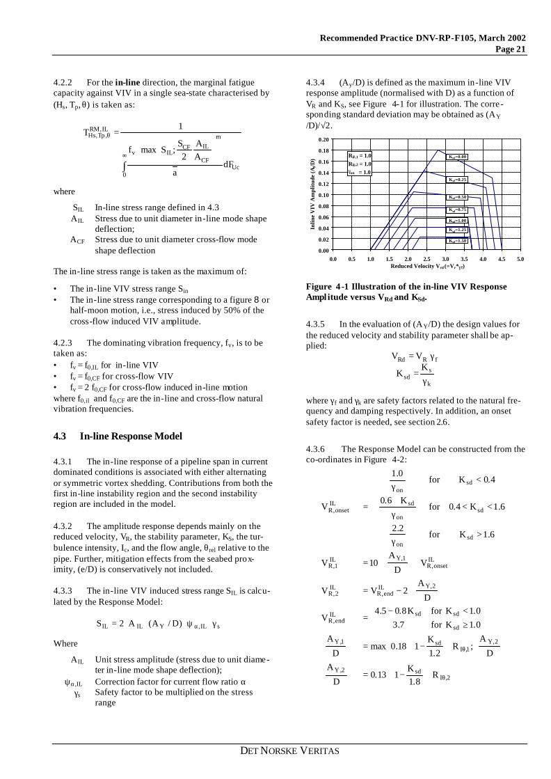
4.3.4 (Ay/D) is defined as the maximum in-line VIV response amplitude (normalised with D) as a function of VR and KS, see Figure 4-1 for illustration. The corre -sponding standard deviation may be obtained as (AY /D)/√2.
0.00
0.02
0.04
0.06
0.08
0.10
0.12
0.14
0.16
0.18
0.20
0.0 0.5 1.0 1.5 2.0 2.5 3.0 3.5 4.0 4.5 5.0
Inlin
e V
IV A
mpl
itud
e (A
y/D) Ksd=0.00
Reduced Velocity Vrd (=Vr*γ f)
Riθ,1 = 1.0Riθ,2 = 1.0γon = 1.0
Ksd=1.50
Ksd=1.25
Ksd=1.00
Ksd=0.75
Ksd=0.50
Ksd=0.25
Figure 4 -1 Illustration of the in-line VIV Response Ampl itude versus VRd and KSd.
4.3.5 In the evaluation of (AY/D) the design values for the reduced velocity and stability parameter shall be ap-plied:
k
ssd
fRRdK
K
VV
γ=
γ=
where γf and γk are safety factors related to the natural fre-quency and damping respectively. In addition, an onset safety factor is needed, see section 2.6.
4.3.6 The Response Model can be constructed from the co-ordinates in Figure 4-2:
2,Isd2,Y
2,Y1,I
sd1,Y
sd
sdsdILend,R
2,YILend,R
IL2,R
ILonset,R
1,YIL1,R
sdon
sdon
sd
sdon
ILonset,R
R8.1
K113.0
D
AD
A;R
2.1K
118.0maxD
A0.1Kfor7.30.1KforK8.05.4
V
D
A2VV
VD
A10V
6.1Kfor2.2
6.1K4.0forK6.0
4.0Kfor0.1
V
θ
θ
⋅
−⋅=
⋅
−⋅=
≥<−
=
⋅−=
+
⋅=
>
γ
<<
γ+
<
γ
=

Recommended Practice DNV-RP-F105, March 2002 Page 22
Inlin
e V
IV A
mpl
itude
DA Y
Reduced Velocity
D
A;V 1,YIL
1,R
D
A;V
2,YIL2,R
)0;V ILend,R
( )0;V ILonset,R
Figure 4 -2 Response Model generation principle.
4.3.7 The reductions RIθ,1(Ic,θrel) and RIθ,2(Ic) accounts for the effect of the turbulence intensity and angle of at-tack (in radians) for the flow, see Figure 4-3.
( )( )
1R017.0
03.0I0.1R
1R003.0I22
1R
2,Ic
2,I
1,Icrel2
1,I
≤≤−
−=
≤≤−
θ⋅−
ππ−=
θθ
θθ
0
0.1
0.2
0.3
0.4
0.5
0.6
0.7
0.8
0.9
1
0 0.02 0.04 0.06 0.08 0.1 0.12 0.14 0.16 0.18 0.2Turbulence Intensity, Ic
R iθ ,2
all angles
Ri θ,1 θrel=30ο
R iθ ,1 θrel=0ο
Ri θ,1 θrel=45ο
Ri θ,1 θrel=60ο
Figure 4-3 Reduction function wrt turbulence intensity and flow angle
4.3.8 ψα,IL is a reduction function to account for re -duced in-line VIV in wave dominated conditions:
>α<α<−α
<α=ψ α 8.0
8.0for0.15.0for3.0/)5.0(
5.0for0.0
IL,
Hence, in case of α < 0.5 in-line VIV may be ignored.
4.4 Cross-flow Response Model
4.4.1 Cross-flow VIV are affected by several parame-ters, such as the reduced velocity VR, the Keulegan-Carpenter number, KC, the current flow velocity ratio, α, the stability parameter, KS, the seabed gap ratio, (e/D), the Strouhal number, St and the pipe roughness, (k/D), among others. Note that Reynolds number, Re, is not explicit in the model.
4.4.2 For steady current dominated flow situations, onset of cross-flow VIV of significant amplitude occurs typically at a value of VR between 3.0 and 5.0, whereas maximum vibration levels occurs at a value of VR between 5 and 7. For pipes with low specific mass, wave dominated flow situations or span scenarios with a low gap ratio, cross-flow vibration may be initiated for VR between 2 and 3.
4.4.3 The cross-flow VIV induced stress range SCF due to a combined current and wave flow is assessed using the following Response Model:
skZCFCF R)D/A(A2S γ⋅⋅⋅⋅=
Where
ACF Unit stress amplitude (stress due to unit diame-ter cross-flow mode shape deflection);
Rk Amplitude reduction factor due to damp-ing
γs Safety factor to be multiplied on the stress range
The cross-flow VIV amplitude (AZ/D) in combined current and wave flow conditions may be taken from Figure 4-4. The figure provides characteristic maximum values. The corresponding standard deviation may be obtained as (AZ /D)/√2.
0.00.10.20.30.40.50.60.70.80.91.01.11.21.31.41.5
0 1 2 3 4 5 6 7 8 9 10 11 12 13 14 15 16
Cro
ss-F
low
VIV
Am
plit
ude
(AZ/
D)
cronset,RV
1.0γ
1.0ψ
1.0ψ
1.0
1.0ψ
on
onseta,
onsetmass,
onsetψ trench,
onsetproxi,
=
=
=
=
=
Reduced Velocity Vrd (=Vr*γ f)
α < 0.8 ; KC < 10
α > 0.8 ; all KC
α < 0.8 ; KC > 30
Figure 4-4 Basic Cross-Flow Response Model

Recommended Practice DNV-RP-F105, March 2002 Page 23
DET NORSKE VERITAS
4.4.4 The amplitude response (AZ/D) as a function of α and KC can be constructed from:
( )
=
≤≤≤α−⋅+
α
=
=
⋅
−=
=γ
ψ⋅ψ⋅ψ⋅ψ⋅= α
DA
DA
30KC9.030KC108.010KC01.07.0
10KC7.0KCall8.03.1
D
A
16VD
A3.1
9VV
5V
3V
1,Z2,Z
1,Z
CFend,R
1,ZCFend,R
CF2,R
CF1,R
on
onset,trenchonset,onset,massonset,proxiCFonset,R
f
pf
Cro
ss-F
low
VIV
Am
plitu
de
Reduced Velocity
D
A;V 2,ZC F
2,R
D
A;V 1,ZC F
1,R
( )1.0;V CFonset,R
)0;VCFend,R
( )0.0;0.2
Figure 4-5 Response Model generation principle
4.4.5 The reduced onset velocity for cross-flow VIV, CF
onset,RV depends on the seabed proximity, trench geometry
and current flow ratio α, whereas the maximum amplitude is a function of α and KC.
4.4.6 ψproxi,onset is a correction factor accounting for the seabed proximity:
<+=ψ
else1
8.0De
for)De
25.13(41
onset,proxi
4.4.7 ψmass,onset is a correction factor accounting for the specific mass (gravity) of the pipe:
<ρρ
ρρ
+=ψelse1
5.1for31
21 ss
onset,mass
where ρs/ρ is the specific mass.
4.4.8 ψα,onset is a correction factor accounting for the current wave ratio:
<αα+=ψ α
else167.1
5.0for3
1onset,
4.4.9 ψtrench,onset is a correction factor accounting for the effect of a pipe located in/over a trench:
D5.01onset,trench
∆+=ψ
where ∆/D denotes a relative trench depth given by:
1D
0where
Ded25.1
D
≤∆≤
−=
∆
The trench depth d is to be taken at a width equal to 3 outer diameters. ∆/D = 0 corresponds to a flat seabed or a pipe located in excess of D/4 above the trench, i.e. the pipe is not affected by the presence of the trench, see Figure 4-6. The restriction ∆/D < 1.0 is applied in order to limit the relative trench depth
d
D
e
3D
Figure 4-6 Definition of Trench Factor
4.4.10 The characteristic amplitude response for cross-flow VIV may be reduced due to the effect of damping. The reduction factor, Rk is given by:
≤−
= − 4Kfor 4Kfor
K3.2K15.01
Rsd
sd5.1
sd
sdk f
4.4.11 The normalised amplitude curves in Figure 4-4 to a large degree embody all available test result. In addition, the following comments apply: • The response for small gap ratio (e/D<< 1) is associ-
ated with one-sided vortex shedding and may not be characterised by VIV parameters as VR and KC. How-ever, the indicated response curve is considered con-servative in general.
• The response for low KC numbers in the cross-flow response model are not in a narrow sense related to the VIV phenomena but rather linked to wave induced water particle motions. Typical maximum response at VR between 2.5 and 3.0 occur at Tu/T0≈ 2. Tu is the

Recommended Practice DNV-RP-F105, March 2002 Page 24
wave induced flow period at pipe level and T0 is the natural period.
4.4.12 Potential vibrations at low KC numbers must be accounted for and care should be observed in case:
9KC3and)1(3
KCVR <<
α−⋅>
This corresponds to rare cases where Tu < 3T0. If violated, the criticality should be evaluated using an appropriate force model.

Recommended Practice DNV-RP-F105, March 2002 Page 25
DET NORSKE VERITAS
5 Force Model
5.1 General
5.1.1 In principle, force models may be used for both vortex induced and direct wave and current dominated loads if appropriate formulations of force models exist and reliable and consistent data are available for calibration. For cross-flow VIV, generally applicable force models do not exist and empirical response models presented in 4.4 reflecting observed pipeline response in a variety of flow conditions is at present superior.
5.1.2 A force model based on the well-known Mori-son’s equation for direct in-line loading is considered herein. Both time domain (TD) and frequency domain (FD) solutions are allowed. A time domain solution may account for all significant non-linearities but is in general very time consuming if a large number of sea-states are to be analysed. For fatigue analyses, a frequency domain solution (if thoroughly verified) is more tractable since it facilitates analyses of a very large number of sea-states at a small fraction of the time required for a time domain solution.
5.1.3 In this document, a complete FD approach for short-term fatigue analyses is presented. Recommended procedures for state-of-the-art Time Domain (TD) short-term damage calculation may be found in DNV-OS-F201. A simplified assessment method is given in 5.3.
5.2 FD solution for In-line direction
5.2.1 The recommended FD solution for the short term- fatigue damage due to combined current and direct wave actions in a single sea-state is based on: • Palmgren-Miner approach using SN-curves; • linearisation scheme for drag term in the Morison
equation based on conservation of damage; • effect of co-linear mean current included in linearis a-
tion term; • narrow banded fatigue damage with semi -empirical
correction to account for wide-band characteristic; The formulation presented in this document has been suc-cessfully verified against comprehensive time domain simulations using Rain flow Counting techniques, see e.g. Mørk &Fyrileiv, 1998. The formulation is based on the following assumptions:
• the main damage contribution comes from lowest natural mode, i.e. the excitation frequency is far from the natural frequency for the higher order modes;
• the effective mass, me , and standard deviation of the flow velocity σU is invariant over the free span length, i.e. for span length less than the dominant wavelength.
5.2.2 The short term fatigue capacity against direct wave actions in a single sea-state characterised by (Hs, Tp, θ) is given in the following form:
ss
)mm(
2
1
1RFC
2RFC
12
sw22
2sw1
1
1RFCv
m1FM
,T,H
22S
Sa
a)m()m(
SS
,2
m1G
SS
,2
m1G
)m(fSa
T
12
1
PS
γ⋅σ=κκ
=χ
+⋅χ+
+
×κ⋅
⋅=
−
−
−
θ
Where σS Standard deviation of stress amplitude fv Vibration frequency
21 a,a Fatigue constant; see 2.4.3
m1 , m2 Fatigue exponent; see 2.4.3 Ssw Stress range, for which change in slope oc-
curs; see 2.4.3
( )x,G 1 ϕ
∫=∞
−ϕ−
x
1t dtte is the
Complementary incomplete Gamma function
)x,(G 2 ϕ ∫= −ϕ−x
0
1t dtte is the
Incomplete Gamma function γs Safety factor on stress range, see 2.6
5.2.3 The standard deviation of the wave induced stress amplitude σS is given by the square root of the spectral moment of the 0th order defined by 5.2.6.
0S M=σ
5.2.4 The characteristic vibration frequency of consid-ered pipe stress response, fv, is taken equal to the mean up-crossing frequency defined by:
0
2v M
M21
fπ
≈
M0 and M2 is defined by 5.2.6.
5.2.5 The rain flow counting correction factor, κRFC, accounts for the “exact” wide-banded damage, i.e. correct-ing the implicit narrow-banded Rayleigh assumption for the stress amplitudes to provide results similar to those arising from a state-of-the-art rain flow counting tech-nique. The Rain Flow Counting factor κRFC is given by:
323.2m587.1bm033.0926.0a
where)1)(a1(a)m( b
RFC
−=−=
ε−−+=κ
κ
κ
κκκ

Recommended Practice DNV-RP-F105, March 2002 Page 26
The bandwidth parameter ε is defined by:
40
22
MMM
1−=ε
The process (spectrum) is narrow-banded for ε → 0 and broad banded for ε → 1 (in practice the process may be considered broad-banded for ε larger than 0.6).
5.2.6 The n th response spectral moment is given by:
∫∞
ωωω=0
SSn
n d)(SM
Where SSS(ω) is the one-sided stress response spectral density function given by:
( )
( )20T
2220
2e
2max
22I
22D
22DSS
)2()(m
)(S)(GggbR)(S
ωωζ+ω−ω
λ
×ω⋅ω⋅ω+⋅=ω ηη
Where
RD Factor accounting for the wave spreading and direction; see 3.4.3.
b Linearisation constant; see 5.2.8. gD Drag force term; see 5.4.1. gI Inertia force term; see 5.4.1. G(ω) Frequency transfer function; see 3.3 Sηη Single -sided wave elevation spectrum; see 3.3 ω0 = 2πf0/γf is the angular natural frequency ζT Total damping ratio fro m
• structural damping; see 6.3.10 • soil damping; see 7.2.10. • hydrodynamic damping; see 5.2.9.
me Effective mass per unit length incl. added mass; see 6.8.3
5.2.7 λmax is an equivalent stress factor given by:
( ) ( )
∂
φ∂λ
−+=λ
21
2
L1
smax
xmax2
EtDCSF1
φ1 (x)) 1st mode shape E Young’s modulus
CSF Concrete stiffness factor; see 6.3.5 Ds Outer steel pipe diameter t Pipe wall thickness L Length of mode shape λ1 Mode shape weighting factor given by:
∫
∫
φ
φ=λ
L
0
21
L
01
1
dx)x(
dx)x(
λ1 is typically in the order of 1.3
In lieu of more detailed data, λmax may be taken as:
1IL
max DA
λ=λ
where A IL is given by 6.8.4.
5.2.8 The linearisation constant b is given by:
)U
(g11.2bu
ccu σ
⋅σ⋅=
where Uc is the mean current and σu=Uw/2 is the standard deviation of the wave induced flow velocity. gc(•) is a cor-rection function accounting for the effect of a steady cur-rent given by:
( ) ( )
( )
∫ ∞−
−
π
−
ϕ=Φ
=ϕ
Φ⋅+ϕπ=
x
x21
2
1
c
dx)x()x(
ex
;21xxx2)x(g
2
ϕ(x) is the Gaussian probability density function and Φ(x) is the corresponding distribution function.
5.2.9 The (linearized) hydrodynamic damping ratio ζh is given by:
1U
c0e
Duh
U
Cgfmg
2
1λ
σ
π=ζ
σ
5.3 Simplified Fatigue Assessment
5.3.1 In situations where quasi-static stress response can be assumed (when the wave period is far larger than the natural vibration period of the span), a simplified fa-tigue assessment may be tractable rather than a complete TD or FD approach.
In such cases, the short term fatigue capacity against direct wave actions in a single sea-state characterised by (Hs, Tp, θ) may be estimated as follows: (cf. 2.4.5)
umFM
,T,H TSaTPS
−θ ⋅=
where S is the quasi-static stress range response from a direct regular wave load at pipe level using Morison’s equation. Tu is the mean zero upcrossing period in 3.3.6.
5.4 Force Coefficients
5.4.1 The force P(x,t) per unit length of a pipe free span is represented by the Morison’s equation. Assuming that the velocity of the structure is not negligible compared with the water particle velocity Morison’s equation reads:
( ) yD4
CUgyUyUg)t,x(P 2aID &&&&& ρ
π−+−−=

Recommended Practice DNV-RP-F105, March 2002 Page 27
DET NORSKE VERITAS
where
ρ Water density D Outer pipe diameter U Instantaneous (time dependent) flow ve-
locity y Pipe lateral displacement gD = 0.5ρDCD is the drag force term gI = M
24
CDρπ is the inertia force term
5.4.2 The added mass term in the Morison equation
zD4
C 2a &&ρπ is assumed implicit in the effective mass me , see
6.7.1.
5.4.3 The drag coefficient CD and inertia coefficient CM to be used in Morisons equation is a function of : • the Keulegan Carpenter number, KC; • the current flow ratio, α; • the gap ratio, (e/D); • the trench depth, (∆/D); • Reynolds number, Re; • the pipe roughness, (k/D); In addition also the cross-flow vibration level, (Az/D) in -fluences the drag coefficient. Note that the dependency of the Reynolds number is embedded in the cylinder rough-ness effect.
5.4.4 The drag coefficient CD is to be taken as
CD,ACD,trenchCD,proxiCD,k0,DD CC ψ⋅ψ⋅ψ⋅ψ⋅=
5.4.5 CD,0 is the basic drag coefficient in oscillatory flow for a free concrete coated pipe (KC>5):
( )
α+
≤α+α−⋅=
5.0KC545.0
5.0KC5
19.0C 0,D
f
For pure current CD,0 = 0.45 (i.e., for KC→∝).
0.0
0.2
0.4
0.6
0.8
1.0
1.2
1.4
1.6
1.8
2.0
0 5 10 15 20 25 30 35 40
KC
Dra
g C
oef
fici
ent C
D
0.1
0.10.1
0.1
CD,A
CD,trench
CD,proxi
CD,k
=ψ
=ψ=ψ
=ψ
α 0.0 0.1 0.2 0.3 0.4 0.5
Figure 5-1 Drag coefficient CD versus KC and α
The drag load is often of small practical importance for small KC values and CD,0 may be interpolated for com-pleteness for KC < 5, see Figure 5-1.
5.4.6 ψproxi,CD is a correction factor accounting for the seabed proximity:
( )
<
⋅++=ψ
else1
8.0e/Dfor )D/e(51
5.09.0
CD,proxi
5.4.7 CD,kψ is a correction factor for the pipe rough-
ness.
⋅+=ψ
Dk
ln05.025.1CD,k
In lieu of detailed documentation of the surface roughness the following values may be applied:
Pipe surface k [metres]
Steel, painted 10-6
Steel, un-coated (not rusted) 10-5
Concrete 1/300
Marine growth 1/200 → 1/20
5.4.8 ψtrench,CD is a correction factor accounting for the effect of a pipe in a trench:
∆
−=ψD3
21CD,trench
∆/D is the relative trench depth given by 4.4.9.
5.4.9 ψA,CD is an amplification factor due to cross-flow vibrations, i.e., proportional to increased projected area to mean flow.
⋅+=ψ
D
A21 y
CD,A
5.4.10 The inertia coefficient CM is to be taken as:
CM,trenchCM,proxiCM,k0,MM CC ψ⋅ψ⋅ψ⋅=
5.4.11 CM,0 is the basic inertia coefficient for a free con-crete coated pipe taken as, see Figure 5-2:
( )( )
α≤αα⋅−
=α
+α−⋅
+α=
5.06.05.026.1
)(f
5KC)(f25
)(fC 0,M
f

Recommended Practice DNV- RP- F105, March 2002 Page 28
0.0
0.2
0.4
0.6
0.8
1.0
1.2
1.4
1.6
1.8
2.0
0 5 10 15 20 25 30 35 40
KC
Iner
tia
Co
effi
cien
t CM
α 0.0 0.1 0.2 0.3 0.4 0.5
1.0ψ1.0ψ
1.0ψ
CMtrench,
CMproxi,
CMk,
=
=
=
Figure 5-2 Inertia coefficient CM versus KC and α
5.4.12 CM,kψ is a correction factor accounting for the
pipe roughness.
CD,kCM,k 2 ψ−=ψ
5.4.13 ψproxi,M is a correction factor accounting for the seabed proximity:
( )
<
⋅++
=ψelse1
8.0e/Dfor )D/e(51
8.084.0M,proxi
5.4.14 ψtrench,M is a correction factor accounting for the effect of a pipe in a trench:
∆
−=ψD3
11M,trench
∆/D is the relative trench depth given by 4.4.9

Recommended Practice DNV-RP-F105, March 2002 Page 29
DET NORSKE VERITAS
6 Structural Analysis
6.1 General
6.1.1 The following tasks are normally required for assessment of free spans: • structural modelling • modelling of pipe-soil interaction • load modelling • a static analysis to obtain the static configuration of
the pipeline • an eigenvalue analysis which provides natural fre-
quencies and corresponding modal shapes for the in-line and cross-flow vibrations of the free spans
• a response analysis using a response model or a force model in order to obtain the stress ranges from envi-ronmental actions.
6.2 Morphological classification
6.2.1 The objective of the morphological classification is to define whether the free span is isolated or interacting. The morphological classification determines the degree of complexity required of the free span analysis: • two or more consecutive free spans are considered to
be isolated (i.e. single span) if the static and dynamic behaviour are unaffected by neighbouring spans;
• a sequence of free spans is interacting (i.e. multi-spanning) if the static and dynamic behaviour is af-fected by the presence of neighbouring spans. If the free span is interacting, more than one span must be included in the pipe/seabed model.
6.2.2 The morphological classification should in gen-eral be determined based on detailed static and dynamic analyses. The classification may be useful for evaluation of scour induced free spans and in application of approxi-mate response quantities. In lieu of detailed data, Figure 6-1 may be used to classify the spans into isolated or interacting dependent on the soil types and span and support lengths.
0.0
0.1
0.2
0.3
0.4
0.5
0.6
0.7
0.8
0.9
1.0
1.1
0.0 0.1 0.2 0.3 0.4 0.5 0.6 0.7 0.8 0.9 1.0Relative span shoulder length, Lsh/L
Rel
ativ
e le
ng
th o
f ad
jaen
t sp
an, L a
/L
La Lsh L
Isolated
Interacting
very soft clay
soft/firm clay
stiff clay
sand
Figure 6-1 Classification of free spans
The curves are, in strict terms, only valid for the vertical (cross-flow) dynamic response but may also be used for assessment of the horizontal (in-line) response.
6.3 Structural modelling
6.3.1 The structural behaviour of the pipeline shall be evaluated by modelling the pipeline, seabed and relevant artificial supports and performing static and dynamic analyses. This section presents requirements for the struc-tural modelling. Soil-pipe interactions are treated in section 7.
6.3.2 A realistic characterisation of the cross-sectional behaviour of a pipeline can be based on the following as-sumptions: • the pipe cross-sections remain circular and plane; • the stresses may be assumed constant across the pipe-
wall thickness; • load effect calculation is normally to be performed
using nominal un-corroded cross section values; • the application of this document is limited to elastic
response, hence plasticity models and effects of two-dimensional state of stress (axial and hoop) on bend-ing stiffness need not be considered.
6.3.3 The effect of coating is generally limited to in-creasing submerged weight, drag forces, added mass or buoyancy. The positive effect on the stiffness and strength, see 6.3.5, is normally to be disregarded. If the contribution of the coating to the structural response is considered sig-nificant, appropriate models shall be used.
6.3.4 Non-homogeneity of the bending stiffness along the pipe, due to discontinuities of the coating across field joints or other effects, may imply strain concentrations that shall be taken into account.
6.3.5 The stiffening effect of concrete coating may be accounted for by:
75.0
steel
concc EI
EIkCSF
=
where CSF denotes the stiffness of concrete coating rela-tive to the steel pipe stiffness and (1+CSF) is the stress concentration factor due to the concrete coating and local-ised bending. The parameter kc is an empirical constant accounting for the deformation/slippage in the corrosion coating and the cracking of the concrete coating. The value of kc may be taken as 0.33 for asphalt and 0.25 for PP/PE coating.
In case the increased stiffness effect is utilised, the in-creased bending stresses due to field joints must also be accounted for.
The CSF given above is assumed valid for all relevant pipe diameters, D/t-ratios and concrete strengths, fcn, provided that that the pipe joint length exceeds 12m, the field joint

Recommended Practice DNV-RP-F105, March 2002 Page 30
length is 0.5-1.0m and the concrete coating thickness does not exceed 150mm.
6.3.6 In lieu of detailed data, it is conservative to as-sume that a girth weld is present in the most heavily loaded cross-section. This is also a basis for the concrete stiffening effect given above.
6.3.7 The cross-sectional bending stiffness of the con-crete coating, EIconc, is the initial, uncracked stiffness. Young’s modulus for concrete may be taken as:
3.010000 cnconc fE ⋅=
where fcn is the construction strength of the concrete. Both Econc and fcn are to be in N/mm2.
6.3.8 The boundary conditions applied at the ends of the pipeline section modelled shall be able to simulate the pipe-soil interaction and the continuity of the pipeline. Sufficient lengths of the pipeline at both sides of the span must be included in the model to account for the effects of side spans, if relevant.
6.3.9 The element length to be used in a finite element model is dictated by the accuracy required. If the stress ranges are to be derived from the mode shapes, see 6.8.4, the accuracy of the stress ranges becomes strongly affected by the element length, especially at the span shoulders.
Ideally the maximum element length should be found by reducing the length until the results (natural frequencies and stresses) converge towards constant values. In practice this may be difficult to perform and, as guidance, the ele-ment length should be in the order of the outer diameter of the pipeline (1D). However, higher order modes and/or short spans (L/Ds < 30) may require shorter elements.
6.3.10 Structural damping is due to internal friction forces of the pipe material and depends on the strain level and associated deflections. If no information is available, a structural modal damping ratio of
ζstr = 0.005
can be assumed. If concrete coating is present, the sliding at the interface between concrete and corrosion coating may further increase the damping to typically 0.01-0.02.
6.3.11 It is recommended to verify the finite element modelling and the post-processing by comparing the re-sults from the finite element analysis with the approximate response quantities of section 6.8 for a single span with zero effective axial force and L/Ds = 60. The in-line and cross-flow natural frequencies and stress ranges shall show similar values within ±5%.
6.3.12 ULS conditions may require a more refined pipe-soil modelling than the linearized eigen-value analysis due to sliding at the span supports.
6.4 Functional Loads
6.4.1 The functional loads which shall be considered are: • weight of the pipe and internal fluid; • external and internal fluid pressure; • thermal expansion and contraction, and • residual installation forces.
6.4.2 Response calculations must account for the rele -vant sequence of load application, if important.
6.5 Static analysis
6.5.1 The static configuration is to be determined for the following conditions if relevant: • as-laid condition; • flooded condition; • pressure test condition, and • operating condition.
6.5.2 The static analysis should normally account for non-linear effects such as: • large displacements (geometric non-linearity); • soil non-linear response, and • loading sequence.
6.5.3 The stiffness of the pipeline consists of material stiffness and geometrical stiffness. The geometrical stiff-ness is governed by the effective axial force, Seff. This force is equal to the true steel wall axial force, Ntr, with corrections for the effect of external and internal pressures:
eeiitreff ApApNS +−=
Where
Ntr “True” steel wall axial force pi Internal pressure pe External pressure Ai Internal pipe (bore) cross section area Ae External pipe (incl. Coating) cross section area
The effective axial force in a span is difficult to estimate due to uncertainties in operational temperature and pres-sure, residual lay tension and axial force relaxation by sagging, axial sliding (feed-in), lateral buckling, multi-spanning and significant seabed unevenness. All these effects should be considered and taken into account if relevant. Then the most reliable method to estimate the effective axial force is use of non-linear FE analysis. As boundary values, the effective axial force for a completely unrestrained (axially) pipe becomes:
0=effS
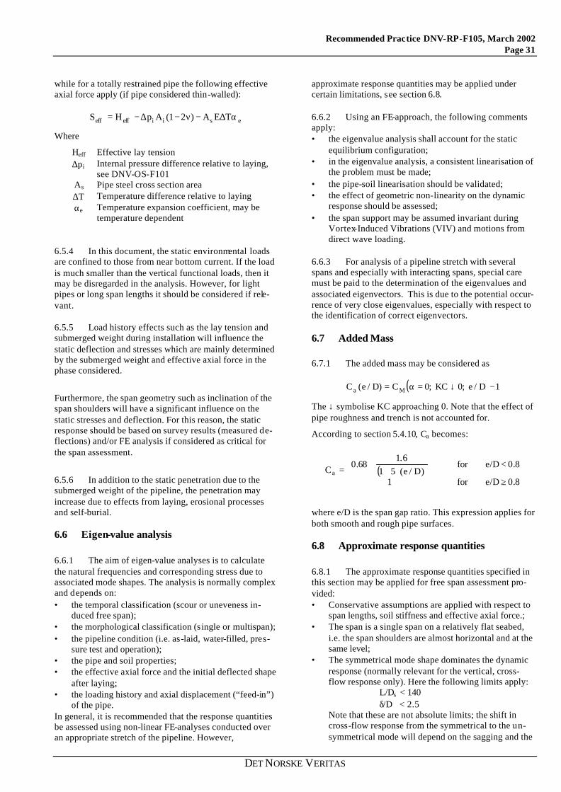
Recommended Practice DNV-RP-F105, March 2002 Page 31
DET NORSKE VERITAS
while for a totally restrained pipe the following effective axial force apply (if pipe considered thin-walled):
esiieffeff TEA)21(ApHS α∆−ν−∆−=
Where
Heff Effective lay tension ∆pi Internal pressure difference relative to laying,
see DNV-OS-F101 As Pipe steel cross section area ∆T Temperature difference relative to laying αe Temperature expansion coefficient, may be
temperature dependent
6.5.4 In this document, the static environmental loads are confined to those from near bottom current. If the load is much smaller than the vertical functional loads, then it may be disregarded in the analysis. However, for light pipes or long span lengths it should be considered if rele-vant.
6.5.5 Load history effects such as the lay tension and submerged weight during installation will influence the static deflection and stresses which are mainly determined by the submerged weight and effective axial force in the phase considered.
Furthermore, the span geometry such as inclination of the span shoulders will have a significant influence on the static stresses and deflection. For this reason, the static response should be based on survey results (measured de-flections) and/or FE analysis if considered as critical for the span assessment.
6.5.6 In addition to the static penetration due to the submerged weight of the pipeline, the penetration may increase due to effects from laying, erosional processes and self-burial.
6.6 Eigen-value analysis
6.6.1 The aim of eigen-value analyses is to calculate the natural frequencies and corresponding stress due to associated mode shapes. The analysis is normally complex and depends on: • the temporal classification (scour or uneveness in-
duced free span); • the morphological classification (single or multispan); • the pipeline condition (i.e. as-laid, water-filled, pres-
sure test and operation); • the pipe and soil properties; • the effective axial force and the initial deflected shape
after laying; • the loading history and axial displacement (“feed-in”)
of the pipe. In general, it is recommended that the response quantities be assessed using non-linear FE-analyses conducted over an appropriate stretch of the pipeline. However,
approximate response quantities may be applied under certain limitations, see section 6.8.
6.6.2 Using an FE-approach, the following comments apply: • the eigenvalue analysis shall account for the static
equilibrium configuration; • in the eigenvalue analysis, a consistent linearisation of
the problem must be made; • the pipe-soil linearisation should be validated; • the effect of geometric non-linearity on the dynamic
response should be assessed; • the span support may be assumed invariant during
Vortex-Induced Vibrations (VIV) and motions from direct wave loading.
6.6.3 For analysis of a pipeline stretch with several spans and especially with interacting spans, special care must be paid to the determination of the eigenvalues and associated eigenvectors. This is due to the potential occur-rence of very close eigenvalues, especially with respect to the identification of correct eigenvectors.
6.7 Added Mass
6.7.1 The added mass may be considered as
( ) 1D/e;0KC;0C)D/e(C Ma −↓=α=
The ↓ symbolise KC approaching 0. Note that the effect of pipe roughness and trench is not accounted for.
According to section 5.4.10, Ca becomes:
( )
≥
<⋅+
+=8.0e/Dfor 1
8.0e/Dfor )D/e(51
6.168.0Ca
where e/D is the span gap ratio. This expression applies for both smooth and rough pipe surfaces.
6.8 Approximate response quantities
6.8.1 The approximate response quantities specified in this section may be applied for free span assessment pro-vided: • Conservative assumptions are applied with respect to
span lengths, soil stiffness and effective axial force.; • The span is a single span on a relatively flat seabed,
i.e. the span shoulders are almost horizontal and at the same level;
• The symmetrical mode shape dominates the dynamic response (normally relevant for the vertical, cross-flow response only). Here the following limits apply:
L/Ds < 140 δ/D < 2.5
Note that these are not absolute limits; the shift in cross-flow response from the symmetrical to the un-symmetrical mode will depend on the sagging and the

Recommended Practice DNV-RP-F105, March 2002 Page 32
levelling/inclination of the span shoulders. In cases where a shift in the cross-flow response is considered as likely, the structural response of the span should be assessed by using FE analysis including all important aspects;
• Bar buckling is not influencing on the response, i.e. C2Seff/PE > -0.5;
• A sensitivity study is performed in order to quantify the criticality of the assumptions.
Approximate response quantities are considered relevant in performing efficient screening of FE or survey results in order to identify critical spans to be assessed with methods that are more accurate, see Fyrileiv & Mørk, (1998).
6.8.2 The fundamental natural frequency may be ap-proximated by:
δ
+⋅+⋅+⋅≈2
3E
eff24
effe10 D
CP
SC1
LmEI
CSF1Cf
where
C1 – C3 Boundary condition coefficients E Youngs modulus for steel I Moment of inertia for steel
CSF Concrete stiffness enhancement factor Leff Effective span length, see 6.8.9 me Effective mass, see below D Outer diameter of pipe PE Euler buckling load = (1+CSF)π2 EI/Leff
2 (positive sign)
δ Static deflection, normally ignored for in-line direction). Shall be limited to 4D.
Seff Effective axial force (negative in compres-sion) , see section 6.5
6.8.3 The effective mass, me, is defined by
φ
φ=
∫
∫
L
2L
2
e ds)s(
ds)s()s(mm
where φ(s) is the assumed mode shape satisfying the boundary conditions and m(s) is the mass per unit length including structural mass, added mass and mass of internal fluid.
6.8.4 The unit diameter stress amplitude (stress due to unit outer diameter mode shape deflection) may be calcu-lated by:
κκ== s
sCF/IL DED
21
2D
IEI
DA
where Ds is the steel pipe diameter and D is the outer pipe diameter (including any coating). κ is the curvature of the assumed mode shape satisfying the boundary conditions mode shape:
2/32
2
2
x1
x)x(
−
∂φ∂
+∂
φ∂=κ
6.8.5 In lieu of detailed information, the (unit diameter) stress amplitude A IL/CF may be estimated by:
( )
( )2eff
s4
max2
2s
CF/IL
L
E)tD(DCSF1C
x2E)tD(D
CSF1A
⋅−⋅+=
∂
φ∂⋅−⋅+=
where t is the steel pipe wall thickness and C4 is a bound-ary condition coefficient.
6.8.6 The static bending moment may be estimated by:
⋅+
⋅=
E
eff2
2eff
5static
PSC1
LqCM
where q represents the loading, i.e. the submerged weight of the pipe in the vertical (cross-flow) direction and/or the drag loading in the horizontal (in-line) direction, see 5.4.1. Note that Leff shall be calculated using the static soil stiff-ness in the Leff/L calculation. Note that, due to historical effects and the local seabed geometry, there is a large uncertainty associated with this simplified expression, see 6.5.5. Note that the term Seff/PE becomes negative when the ef-fective axial force is in compression since PE is defined as positive.
6.8.7 In case the static deflection is not given by direct measurement (survey) or estimated by accurate analytical tools, it may be estimated by:
⋅+
+⋅⋅
=δ
E
eff2
4eff
6
PS
C1
1)CSF1(EI
LqC
where C6 is a boundary condition coefficient. Note that Leff shall be calculated using the static soil stiff-ness in the Leff/L calculation. Note that, due to historical effects and the local seabed geometry, there is a large uncertainty associated with this simplified expression, see 6.5.5.
6.8.8 The coefficients C1 to C6 are given in the table below for different boundary conditions. For multi-spanning scenarios the choice of coefficient should be supported by dedicated FE-analyses.

Recommended Practice DNV-RP-F105, March 2002 Page 33
DET NORSKE VERITAS
Table 6-1 Boundary conditions coefficients Pinned-
Pinned 2) Fixed-Fixed 3)
Single span on seabed
C1 1.57 3.56 3.56
C2 1.00 0.25 0.25 C3
0.8 1) 0.2 1) 0.4 1) C4 4.39 14.1 Shoulder: 14.1(L/Leff)
2 Mid-span: 8.6
C5 1/8 1/12 Shoulder:
6)L/L(181
2eff −
Mid-span: 1/24 C6 5/384 1/384 1/384
1) Note that C3=0 is normally assumed for in-line if the steady current is not accounted for.
2) For pinned-pinned boundary condition Leff is to be replaced by L in the above expressions also for PE.
3) For fixed-fixed boundary conditions, Leff/L=1 per definition.
4) C5 shall be calculated using the static soil stiffness in the Leff/L calculation.
6.8.9 The Leff/L term used above accounts for the effec-tive span length in order to consider the span as fully fixed. This ratio decreases as the L/Ds ratio and soil stiff-ness increase. The Leff/L term is given by (for reference see Hobbs, 1986):
7.2
7.2
for
for
0.161.0036.0
73.4
63.002.1066.0
73.4
LL
2
2
eff
<β
≥β
+β+β
+β+β−=
+⋅
=βEI)CSF1(
LKlog
4
10
where K is the relevant soil stiffness (vertical or horizon-tal, static or dynamic).
6.8.10 The boundary coefficients in Table 6-1 based on the effective span length are found appropriate for fatigue assessment (FLS) under the assumption of small displace-ments. For the check of maximum bending moments (ULS) due to direct wave loading, the pinned-pinned boundary condition may be applied in combination with the apparent span length (not the effective span length).

Recommended Practice DNV-RP-F105, March 2002 Page 34
7 Pipe-soil interaction
7.1 General
7.1.1 The soil is to be classified as cohesive (clays) or cohesionless (sands). As basis for the evaluations of the pipe-soil interaction the following basic soil parameters are relevant: • type of soil; • in-situ stress conditions; • shear strength parameters for drained or undrained
condition including remoulded shear strength for clays;
• soil moduli and damping coefficients as function of cyclic shear strain;
• soil settlement parameters; • general soil data as submerged unit weight, void ratio,
water content and plasticity limits.
7.1.2 If the approximate soil stiffness expressions in 7.3 are to be used, then the following specific parameters are relevant: • submerged unit weight of soil, γsoil’ • Poisson’s ratio, ν • void ratio, es • angle of friction, cohesionless soils, ϕs • undrained shear strength, cohesive soils, su • over-consolidation ratio, OCR • plasticity index, cohesive soils, ip The plasticity index ip is a standard geotechnical parame-ter whose value is usually specified in the soil reports for the pipeline route. The plasticity index influences the dy-namic spring stiffness given in Section 7.3 only for clay and only when the over-consolidation ratio of the clay is greater than one, OCR > 1. Note that OCR > 1 is rarely assumed.
7.1.3 The parameters listed above should preferably be obtained by means of geotechnical tests on undisturbed soil samples and be representative for the particular geo-graphical location of the pipeline. In lieu of detailed in -formation, the values given in Table 7-1 and Table 7-2 may be used.
Table 7-1 Typical geotechnical parameters for sand Soil type ϕs γsoil’
[kN/m3] ν es
Loose 28-30o 8.5-11.0 0.35 0.7-0.9 Medium 30-36o 9.0-12.5 0.35 0.5-0.8 Dense 36-41o 10.0-13.5 0.35 0.4-0.6
Table 7-2 Typical geotechnical parameters for clay Soil type su
[kN/m2] γsoil’
[kN/m3] ν es
Very soft <12.5 4-7 0.45 1.0-3.0 Soft 12.5-25 5-8 0.45 0.8-2.5 Firm 25-50 6-11 0.45 0.5-2.0 Stiff 50-100 7-12 0.45 0.4-1.7
Very stiff 100-200 10-13 0.45 0.3-0.9 Hard >200 10-13 0.45 0.3-0.9
7.1.4 Uncertainties in the soil data should be consid-ered, e.g. by sensitivity analysis. These uncertainties may arise from variations in the soil conditions along the pipe-line route and difficulties in determining reliable in-situ soil characteristics of the upper soil layer, which is the soil of most importance for the pipeline. Soil data down to a depth equal to about 0.5-1.0 times the pipe diameter are most important to consider in this context.
7.2 Modelling of pipe -soil interaction
7.2.1 The pipe-soil interaction is important in the evaluation of the static equilibrium configuration and the dynamic response of a free spanning pipeline. The follow-ing functional requirements apply for the modelling of soil resistance: • the seabed topography along the pipeline route must
be represented; • the modelling of soil resistance must account for non-
linear contact forces normal to the pipeline and lift off;
• the modelling of soil resistance must account for slid-ing in the axial direction. For force models this also applies in the lateral direction;
• appropriate (different) short- and long-term character-istics for stiffness and damping shall be applied, i.e. static and dynamic stiffness and damping.
7.2.2 The seabed topography may be defined by a ver-tical profile along the pipeline route. The spacing of the data points characterising the profile should relate to the actual roughness of the seabed.
7.2.3 The axial and lateral frictional coefficients be-tween the pipe and the seabed shall reflect the actual sea-bed condition, the roughness, the pipe, and the passive soil resistance.
7.2.4 The axial and lateral resistance is not always of a pure frictional type. Rapid changes in vertical stresses are (in low-permeable soil) reacted by pore water and not by a change in effective contact stresses between the soil and the pipe. In addition, the lateral resistance will have a con-tribution due to the penetration of the pipe into the soil, which needs be accounted for.

Recommended Practice DNV-RP-F105, March 2002 Page 35
DET NORSKE VERITAS
7.2.5 For sands with low content of fines, the frictional component of the axial and lateral resistance is propor-tional with the vertical force at any time. For clays, the frictional component is proportional with the undrained shear strength.
7.2.6 Where linear soil stiffness has to be defined for the eigenvalue analysis, the soil stiffness should be s e-lected considering the actual soil resistance and the ampli-tude of the oscillations.
7.2.7 The soil stiffness for vertical loading should be evaluated differently for static and dynamic analyses. The static soil response will be governed mainly by the maxi-mum reaction, including some cyclic effects. Dynamic stiffness will be characterised mainly by the unloading/re-loading situation.
7.2.8 The soil damping is generally dependent on the dynamic loads acting on the soil. Two different types of soil damping mechanisms can be distinguished: • Material damping associated with hysteresis taking
place close to the yield zone in contact with the pipe. • Radiation damping associated with propagation of
elastic waves through the yield zone.
7.2.9 The radiation damping may be evaluated from available solutions for elastic soils using relevant soil modulus reflecting the soil stress (or strain) levels. The radiation damping depends highly on the frequency of the oscillations, and is more important for high frequency os-cillations.
7.2.10 The modal soil damping ratio, ζsoil, due to thesoil-pipe interaction may be determined by:
φ
φ
π=ζ
∫
∫
L
2L
2
0soil ds)s()s(m
ds)s()s(c
f41
where the soil damping per unit length, c(s), may be de-fined on the basis of an energy balance between the maxi-mum elastic energy stored by the soil during an oscillation cycle and the energy dissipated by a viscous damper in the same cycle. Alternatively, the modal soil damping ratio, ζsoil, may be taken from Table 7-3 or Table 7-4, in which L denotes the length of the free span and D is the outer diameter of the pipeline. Interpolation is allowed. Table 7-3 Modal soil damping ratios (in %) for sand.
Horizontal (in-line) direction
L/D
Vertical (cross-flow) direction
L/D
Sand type
<40 100 >160 <40 100 >160
Loose 3.0 2.0 1.0 2.0 1.4 0.8 Medium 1.5 1.5 1.5 1.2 1.0 0.8 Dense 1.5 1.5 1.5 1.2 1.0 0.8
Note that the sand type is identified by the value of the friction angle ϕs (Table 7-1), and the clay type is identified by the value of the undrained shear strength s u (Table 7-2). For pipes supported by rock, values for the modal soil damping ratios may be taken as for dense sand. Table 7-4 Modal soil damping ratios (in %) for clay.
Horizontal (in-line) direction
L/D
Vertical (cross-flow) direction
L/D
Clay type
<40 100 >160 <40 100 >160 Very soft - Soft 3.0 2.0 1.0 3.0 2.0 1.0 Firm – Stiff 2.0 1.4 0.8 1.2 1.0 0.8 Very stiff - Hard 1.4 1.0 0.6 0.7 0.6 0.5
7.3 Approximate Soil Stiffness
7.3.1 The following expressions may be used for the static vertical soil reaction per unit length as a function of the penetration, v: Rv = γsoil’b(Nqv+0.5Nγb) − sandy soils Rv = b(γsoil’Nqv+Ncsu) − clayey soils Where
B Load distribution width:
>≤−=
0.5Dfor v D0.5Dfor v v)vD(2
D Outer pipe diameter (including any coat-ing)
γsoil’ Submerged unit weight of soil. su Undrained shear strength
The expressions for RV are based on bearing capacity for-mulas for ideal 2-D strip foundations. Note that if these formulas are used to predict the expected penetration v for a given contact pressure RV, they may lead to underestima-tion of the true penetration due to effects of the pipelay process and erosion as well as possible 3-D effects on the shoulder near the free span.
7.3.2 The bearing capacity factors Nc, Nq and Nγ versus the internal friction angle ϕs may be calculated from the following formulas:
sq
sqc
s2sq
tan)1N(5.1N
cot)1N(N
)2
45(tan)tanexp(N
ϕ−=
ϕ−=
ϕ+ϕπ=
γ
For clayey soils the friction angle is set equal to 0°, i.e. Nq = 1.0 and Nc = 5.14.

Recommended Practice DNV-RP-F105, March 2002 Page 36
1
10
100
0 10 20 30 40 50
ϕ[degree]
Nc,
Nq
and
Nγ
Nc
Nγ
Nq
Figure 7-1 Bearing capacity factors Nc, Nq and Nγ ver-sus the internal friction angle ϕs
7.3.3 The maximum static, axial soil reaction per unit length may be taken as:
Ra = Rvµa − sandy soils Ra = min{Rvµa, bτmax} − clayey soils
Where
Rv Vertical static soil reaction given by 7.3.1 µa Axial friction coefficient B Given in 7.3.1
kc =
+
−
200
3.1
2001
61.2pp iiOCR
ip in %
τmax
Soil shear strength:
=
2
2 )1(5.0
−−
bRk
s vcu
7.3.4 The static vertical stiffness is a secant stiffness representative for penetration conditions such as during installation and erosion and during development of free spans.
The static vertical stiffness KV,S is defined as KV,S=RV/v, where RV is the static vertical soil reaction per unit length of pipe and v is the vertical penetration of the pipe re-quired to mobilise this reaction. Unless effects of pipelay and erosion and 3-D shoulder effects are significant, the 2-D approach outlined in 7.3.1 can be used to predict v. Oth-erwise, or when no detailed information is available, the static stiffness value may be taken according to Table 7-7 for sand and Table 7-8 for clay.
7.3.5 The vertical dynamic stiffness KV is defined as KV=∆FV/∆δV, where ∆FV is the incremental vertical force between pipe and soil per unit length of pipe, and ∆δV is
the associated incremental vertical displacement of the pipe.
7.3.6 The lateral (horizontal) dynamic stiffness KL is defined as KL=∆FL/∆δL, where ∆FL is the incremental horizontal force between pipe and soil per unit length of pipe, and ∆δL is the associated incremental horizontal dis-placement of the pipe.
7.3.7 For a detailed determination of KV, the following expression may be applied:
ν−⋅=
1G88.0K v
which is based on elastic halfspace theory for a rectangular foundation under assumption of a pipe length that equals 10 times the contact width between pipe and soil. Pois-son’s ratio ν is given in Table 7-1 and Table 7-2.
7.3.8 For a detailed determination of KL, the following expression may be applied:
)1(G76.0K L ν+⋅⋅=
which is based on elastic halfspace theory for a rectangular foundation under assumption of a pipe length that equals 10 times the contact width between pipe and soil. Pois-son’s ratio ν is given in Table 7-1 and Table 7-2.
7.3.9 For conditions with small-amplitude deforma-tions, the shear modulus for the soil can be taken as:
σ+
−⋅
σ+
−⋅
=clayfor )OCR(
e1)e3(1300
sandfor e1
)e3(2000
Gsk
ss
2s
ss
2s
[kN/m2]
where
σs Effective mean stress (in units of kPa), see 7.3.10.
OCR Over-consolidation ratio es Void ratio ks Coefficient, taken from Figure 7-2
0
0.1
0.2
0.3
0.4
0.5
0 20 40 60 80 100 120 140Plasticity index, i p
ks
Figure 7-2 ks versus plasticity index, ip

Recommended Practice DNV-RP-F105, March 2002 Page 37
DET NORSKE VERITAS
This expression for G, which gives lower-bound values for the initial shear modulus, has been calibrated to measure-ments from free pipeline spans. It is based on an expres-sion for the initial shear modulus, formulated by Hardin and Drnevich (1970) and based on experimental results for a broad range of soil types. For extreme conditions, which can be assumed to cause large deformations, considerably lower G values apply.
7.3.10 The effective mean stress, σs, in the soil at the span supports may be calculated from the stress conditions at a representative depth below the pipe. The representa-tive depth may be assumed equal to the contact width b, which is given in Section 7.3.1. The following formula may then be applied:
)L2L
1(b3q
'b)K1(21
shsoil0S ++γ+=σ
in which K0 Coefficient of earth pressure at rest, usu-
ally K0=0.5 γsoil’ Submerged unit weight soil (kN/m3)
q Submerged weight of pipe per unit length of pipe (kN/m)
Lsh Span support length on one shoulder (for transfer of one-half the weight of the free span)
L Span length Note that for pipes on clay, the clay will not be consoli-dated for the weight of the pipe in the temporary phase immediately after pipelay. For calculations for a pipe on clay in this phase, the formula for σs reduces to
'b)K1(21
soil0S γ+=σ
When detailed information does not exist and the topog-raphical conditions are not complex, the support length ratio Lsh/L may be taken according to Table 7-5 for sand and according to Table 7-6 for clay. Table 7-5 Support length ratio Lsh/L for sand
Sand type Lsh/L Loose 0.3
Medium 0.2 Dense 0.1
Table 7-6 Support length ratio Lsh /L for clay
Clay type Lsh/L Very soft 0.5
Soft 0.4 Firm 0.3 Stiff 0.2
Very stiff 0.1 Hard 0.07
7.3.11 The procedure in Sections 7.3.7-7.3.10 leads to values of the dynamic stiffness KV and KL, which can be considered as lower-bound values for initial small-strain stiffness at either end of the free span, but which are not adjusted for possible non-linear soil behaviour at larger strains.
If there are indications that the values for KV and KL should be different from those produced by this procedure, then the ratio between the assumed pipe length on the shoulder and the contact width may be adjusted from the adopted value of 10. Calculation of the effective mean stress σs from the stress conditions at a different represen-tative depth below the pipe than b may also be considered. Note that, in this context, it is acceptable to distinguish between representative depths for calculation of KV and for calculation of KL.
7.3.12 When normal conditions prevail and when no detailed analysis is carried out for determination of KV and KL for small-strain conditions, the values of these stiff-nesses in units of kN/m/m may be calculated in simplified manner as (D is in units of metre):
D)31
32
(CK sVV +
ρρ
=
D)31
32
(CK sLL +
ρρ
=
in which the coefficients CV and CL are taken according to Table 7-7 and Table 7-8. The soil type, which is used as entry to these tables, is identified by the value of the fric-tion angle ϕs for sand (Table 7-1) and by the value of the undrained shear strength su for clay (Table 7-2).
Table 7-7 Dynamic stiffness factor and static stiffness for pipe-soil interaction in sand. Sand type CV
(kN/m5/2) CL
(kN/m5/2) KV,S
(kN/m/m) Loose 16000 12000 250
Medium 22000 16500 530 Dense 32000 24000 1350
Table 7-8 Dynamic stiffness factor and static stiffness for pipe-soil interaction in clay with OCR=1.
Clay type CV (kN/m5/2)
CL
(kN/m5/2) KV,S
(kN/m/m) Very soft 1200 800 50-100
Soft 2700 1800 160-260 Firm 6000 4000 500-800 Stiff 9000 6000 1000-1600
Very stiff 21000 14000 2000-3000 Hard 24000 16000 2600-4200
7.3.13 The simplified expressions are based on the pro-cedure in Sections 7.3.7-7.3.10 for average properties of the considered soil type in conjunction with an assumed

Recommended Practice DNV-RP-F105, March 2002 Page 38
penetration of 20-40% of the diameter and Lsh/L as given in Table 7-7 and Table 7-8. The simplified expressions for KV and KL, with values of CV and CL given in Table 7-7 and Table 7-8, are valid for dynamic conditions with small-amplitude deformations.
7.3.14 For free spans supported by sand, the lateral dy-namic stiffness KL should be calculated under an assump-tion of loose sand properties in order to properly account for effects of erosion.
7.3.15 For extreme conditions, which can be assumed to cause large deformations on the shoulders, a smaller spring stiffness than that associated with small-strain conditions apply. For vertical loading, this smaller spring stiffness is typically of the same order of magnitude as the static ver-tical stiffness KV,S. For lateral loading, reference is made to Section 7.3.16.
7.3.16 In case of lateral loads large enough to cause slid-ing at the span supports, the following bilinear force-displacement curve, which covers both small-strain condi-tions and extreme displacement conditions, may be applied at span supports on sand and clay:
<≤µµ
−⋅+µ
µ<⋅=
max,LLVL1
VL2VL
VLL1
L FFFfor )kF
y(kF
FFfor ykF
in which
y Lateral displacement of pipe on shoulder FL Lateral force per unit length of pipe at dis-
placement y FL,max Maximum lateral resistance per unit length
of pipe FV Vertical contact force per unit length of
pipe on shoulder µL Lateral friction coefficient k1 Initial stiffness up to mobilisation of full
friction k2 Equivalent stiffness for deformations past
mobilisation of full friction Unless data indicate otherwise, µL=0.6 may be applied for span supports on sand and µL=0.2 for span supports on clay. For supports on sand, the initial stiffness k1 may be taken as equal to the lateral dynamic stiffness KL for loose sand. For supports on clay, the initial stiffness k1 may be taken as equal to the lateral dynamic stiffness KL for the clay type in question. The equivalent stiffness k2 depends on the vertical penetra-tion, v, of the pipe on the shoulder. For span supports on sand, values for k2 are given in Table 7-9.
Table 7-9 Equivalent stiffness, k2, for span supports on sand
v/D k2 (kN/m/m) 0.00 0 0.25 19 0.35 28 0.50 44 1.00 105
For span supports on clay, the equivalent stiffness k2 can be calculated as
3.14.0
soil
uu2 D
vD
ss26.8k
⋅
γ
⋅⋅=−
in which γsoil Total unit weight of soil (=γsoil’+γwater) γsoil’ Submerged unit weight of water γwater Unit weight of water (=10 kN/m3)
v Vertical pipe penetration at span shoulder
For span supports on sand, the maximum lateral resistance per unit length of pipe is
25.12
soilVLmax,L Dv
D'0.5FF
⋅⋅γ⋅+µ=
For span supports on clay, the maximum lateral resistance per unit length of pipe is
3.14.0
soil
uuVLmax,L D
vD
ssD13.4FF
⋅
γ
⋅⋅⋅+µ=−
7.3.17 The axial dynamic soil stiffness is usually not important. However, when long free spans are considered, it is important to include an axial soil-support model with friction and stiffness. If no information is available about the axial dynamic soil stiffness, it may be taken as equal to the lateral dynamic soil stiffness KL as described above.
7.4 Artificial supports
7.4.1 Gravel sleepers can be modelled by modifying the seabed profile, considering the rock dump support shape and applying appropriate stiffness and damping characteristics.
7.4.2 The purpose of mechanical supports is generally to impose locally a pipeline configuration in the vertical and/or transverse directions. Such supports can be mo d-elled by concentrated springs having a defined stiffness, taking into account the soil deformation beneath the sup-port and disregarding the damping effect.

Recommended Practice DNV-RP-F105, March 2002 Page 39
DET NORSKE VERITAS
8 References
Blevins, R.D., “Flow-Induced Vibrations”, Krieger Publishing Company, Florida, 1994
Bruschi, R. & Vitali, L., “Large-Amplitude Oscillations of Geometrically Non-linear Elastic Beams Subjected to Hydrodynamic Excitation”, JOMAE, Vol. 113, May, 1991.
DNV Offshore Standard OS-F101, “Submarine Pipeline Systems”.
DNV Offshore Standard OS-F201, “Dynamic Risers”.
DNV Recommended Practice RP-C203, “Fatigue Strength Analysis of Offshore Steel Structures”.
DNV Classification Note CN 30.5, ”Environmental Conditions and Environmental Loads”.
DNV Recommended Practice RP-E305, “On-bottom Stability Design of Submarine Pipelines”.
Fyrileiv, O. & Mørk, K.J., “Assessment of Free Spanning Pipelines using the DNV Guideline”, ISOPE’98, Montreal, Canada, May 24-29, 1998.
Fyrileiv, O., Mørk, K.J. & Rongved, K. “TOGI Pipeline – Assessment of Non-stationary Free Spans”, OMAE’00, New Orleans, USA, February 14-17, 2000.
Hansen, E.A., Bryndum, M., Mørk, K.J., Verley, R., Sortland, L. & Nes, H.,”Vibrations of Free Spanning Pipeline Located in the Vicinity of a Trench", OMAE'01-4016, Rio de Janeiro, Brazil, June 3-8, 2001.
Hardin, B.O., and V.P. Drnevich, “Shear Modulus and Damping in Soils: I. Measurements and Parameters Effects, II. Design Equations and Curves,” Technical Reports UKY 27-70-CE 2 and 3, College of Engineering, University of Kentucky, Lexington, Kentucky, July 1970.
Hobbs, R.E:, “Influence of Structural Boundary Conditions on pipeline Free Span Dynamics”, OMAE’86, 1986.
Mørk, K.J., Vitali, L. & Verley, R., “The MULTISPAN Project: Design Guideline for Free Spanning Pipelines”, Proc. of OMAE’97 conf., Yokohama, Japan, April 13-17, 1997.
Mørk, K.J. & Fyrileiv, O. “Fatigue Design According to the DNV Gu ideline for Free Spanning Pipelines”, OPT’98, Oslo, Norway, February 23-24, 1998.
Mørk K.J., Fyrileiv, O., Verley, R., Bryndum, M. & Bruschi, R. “Introduction to the DNV Guideline for Free Spanning Pipelines”, OMAE’98, Lisboa, July 6-9, 1998.
Mørk, K.J., Fyrileiv, O., Nes, H. & Sortland, L. “A Strategy for Assessment of Non-Stationary Free Spans”, ISOPE-99, Brest, France, May 30-June 4, 1999.
Sumer B.M. & Fredsøe, J. “Hydrodynamics around Cylindrical Structures”, Advanced Series on Ocean Engineering – Volume 12, World Scientific, London, 1997.
Tura, F., Dumitrescu, A., Bryndum, M. B. & Smeed, P.F. “Guidelines for Free Spanning Pipelines: The GUDESP Project”, OMAE’94, Volume V, pp 247-256, Houston, 1994.