free trade area americas - agecon searchageconsearch.umn.edu/bitstream/33995/1/ae040827.pdfunited...

United StatesDepartment ofAgriculture

EconomicResearchService

AgriculturalEconomicReportNumber 827

Free Trade Area

Americas

U.S. Agricultureand the Free TradeArea of the Americas

U.S. Agriculture and the Free Trade Area of the Americas. Market and TradeDivision, Economic Research Service, U.S. Department of Agriculture. AgriculturalEconomic Report No. 827.

AbstractThe Free Trade Area of the Americas (FTAA), a free trade area under negotiation amongthe United States and 33 countries in the Western Hemisphere, will progressively liber-alize trade and investment in the region. It is scheduled to become effective by the endof 2005. The FTAA will lead to a 6-percent increase in annual U.S. agricultural exportsto the Hemisphere and a 3-percent increase in annual U.S. agricultural imports fromthe Hemisphere. The FTAA will increase annual U.S. agricultural exports and importsworldwide by about $1 billion each. The expansion of U.S. agricultural trade due to theFTAA will result from both the direct effect of trade liberalization and the indirecteffect of accelerated economic growth in increasing agricultural demand in the WesternHemisphere. The FTAA complements the multilateral negotiations in the DohaDevelopment Agenda, which have a broader agenda for agricultural reform.

Keywords: Free Trade Area of the Americas, regional integration, preferential tradearrangements, WTO, sanitary and phytosanitary, tariffs, foreign direct investment, envi-ronment.

ContributorsMary E. Burfisher (editor), H. Christine Bolling, Joseph Cooper, Jason Donovan, MarkGehlhar, Paul Gibson, Stephen Haley, Robert Johansson, William Kost, Barry Krissoff,John Link, Mark Peters, Daniel Pick, Gregory Pompelli, Donna Roberts, ShermanRobinson, David Skully, Karen Thierfelder, Constanza Valdes, John Wainio, andSteven Zahniser.

AcknowledgmentsAppreciation is extended to Praveen Dixit for his role in the development and reviewof this project and to Agnes Prentice for statistical assistance. The authors also grate-fully acknowledge the reviews of Phil Abbott, Mary Bohman, Barbara Chattin, MerrittCluff, Joseph Dewbre, Barbara Fecso, Michael Ferrantino, Carol Goodloe, MunisamyGopinath, Russell Hillberry, Jennifer James, Marcos Jank, Won Koo, Mary LisaMadell, Mary Marchant, Steven Neff, Eric Nichols, Kenneth Reinert, James Rude,Robert Spitzer, Thomas Spreen, James V. Stout, David Tarr, and Zhi Wang. Thanksalso to John Weber and Priscilla Smith, our technical editors, and Victor B. Phillips, Jr.and Curtia Taylor, our graphics designers. Research in this report was funded in part bythe National Research Initiative of USDA’s Cooperative State Research, Education, andExtension Service.

Washington, DC 20036-5831 March 2004

ii ✥ U.S. Agriculture and the Free Trade Area of the Americas-Overview/AER-827 Economic Research Service/USDA

Contents

Executive Summary . . . . . . . . . . . . . . . . . . . . . . . . . . . . . . . . . . . . . . . . . . . . . . . . . . . .iii

Overview . . . . . . . . . . . . . . . . . . . . . . . . . . . . . . . . . . . . . . . . . . . . . . . . . . . . . . . . . . . . .1

Chapter 1: Trade and Welfare Effects of the FTAA . . . . . . . . . . . . . . . . . . . . . . . . . . . .26

Chapter 2: Trade Liberalization in the Western Hemisphere:Impacts on U.S. Agricultural Exports . . . . . . . . . . . . . . . . . . . . . . . . . . . . . . . . . . .39

Chapter 3: Measuring Agricultural Tariff Protection . . . . . . . . . . . . . . . . . . . . . . . . . . .52

Chapter 4: U.S. Sugar in the FTAA . . . . . . . . . . . . . . . . . . . . . . . . . . . . . . . . . . . . . . . .67

Chapter 5: The U.S. Orange Juice Industry in the FTAA . . . . . . . . . . . . . . . . . . . . . . .81

Chapter 6: U.S. Foreign Direct Investment in the Western Hemisphere . . . . . . . . . . .93

Chapter 7: Environmental Issues . . . . . . . . . . . . . . . . . . . . . . . . . . . . . . . . . . . . . . . .100

Chapter 8: Regionalizing the Rules for Sanitary and Phytosanitary Measures . . . . . . . . . . . . . . . . . . . . . . . . . . . . . . . . . . . . . . . . . . . . . .111

Appendix 1-1 . . . . . . . . . . . . . . . . . . . . . . . . . . . . . . . . . . . . . . . . . . . . . . . . . . . . . . . .126

Appendix 2-1 . . . . . . . . . . . . . . . . . . . . . . . . . . . . . . . . . . . . . . . . . . . . . . . . . . . . . . . .129

Appendix 2-2 . . . . . . . . . . . . . . . . . . . . . . . . . . . . . . . . . . . . . . . . . . . . . . . . . . . . . . . .132

Appendix 3-1 . . . . . . . . . . . . . . . . . . . . . . . . . . . . . . . . . . . . . . . . . . . . . . . . . . . . . . . .136

Appendix 4-1 . . . . . . . . . . . . . . . . . . . . . . . . . . . . . . . . . . . . . . . . . . . . . . . . . . . . . . . .138

Appendix 5-1 . . . . . . . . . . . . . . . . . . . . . . . . . . . . . . . . . . . . . . . . . . . . . . . . . . . . . . . .139

Appendix 7-1 . . . . . . . . . . . . . . . . . . . . . . . . . . . . . . . . . . . . . . . . . . . . . . . . . . . . . . . .141

Economic Research Service/USDA U.S. Agriculture and the Free Trade Area of the Americas-Overview/AER-827 ✥ iii

Executive SummaryThe Free Trade Area of the Americas (FTAA) is a free trade area currently under nego-tiation among the United States and 33 countries in the Western Hemisphere. Its objec-tive is to progressively liberalize trade and investment in the region. Negotiations onthe FTAA began in 1998 and are to conclude in 2005, with the agreement scheduled tocome into force by the end of that year. These are the implications of the FTAA forU.S. agriculture:

The FTAA will increase annual U.S. global agricultural exports and imports byabout $1 billion each. Elimination of tariffs on intra-regional trade in agriculture andmanufacturing will increase annual U.S. agricultural exports to other countries in theWestern Hemisphere by $1.4 billion (6 percent) and annual imports from the 33 coun-tries by about $900 million (3 percent). The increased U.S. trade with WesternHemisphere countries will lead to small adjustments in U.S. trade with the rest of theworld.

Agricultural trade in the Western Hemisphere will increase by $4 billion (6 percent).Agriculture will account for about 20 percent of trade expansion in the Hemisphere due tothe FTAA, proportionally larger than its current 9-percent share of merchandise tradeand a reflection that current agricultural tariffs are higher than manufacturing tariffs inmany Western Hemisphere countries, including the United States.

Trade liberalization of both agricultural and manufacturing goods in the FTAA willincrease the welfare (consumer purchasing power) of the Western Hemisphere by$63 billion annually. Free trade will allow a more efficient allocation of productiveresources in the region, and can stimulate productivity gains and economic growth indeveloping countries. The expansion of U.S. agricultural trade due to the FTAA willresult from both the direct effect of trade liberalization and the indirect effect of accel-erated economic growth on increasing agricultural demand in the Western Hemisphere.

The FTAA will have small effects on U.S. agricultural production because trade withthe Western Hemisphere accounts for only a small share of aggregate output, andU.S. tariffs are already low. Production changes in most of the commodity categoriesanalyzed in this report will be less than 1 percent. U.S. export growth will lead to smallincreases in production of rice, oilseeds, oils and fats, and dairy products. U.S. sugarproduction could decline significantly, depending on how the domestic support pro-gram may be modified in response to increased sugar imports from other WesternHemisphere countries. The decline in U.S. orange juice production will be reduced ifU.S. demand for domestic, not-from-concentrate orange juice continues to grow.

The FTAA will add to the benefits that trade liberalization already completed in theWestern Hemisphere has had for U.S. agriculture. The impacts of trade reform havebeen greatest for U.S. agricultural exports to Mexico, which instituted a far-reachingset of unilateral trade reforms before it joined the North American Free TradeAgreement (NAFTA). In 1999, U.S. agricultural exports to Mexico were 2.5 times ($3billion) higher than they would have been in the absence of these trade reforms.NAFTA alone accounted for 20 percent of U.S. agricultural exports to Mexico during1994-99. Many U.S. exports have benefited from Mexican trade liberalization, includ-ing wheat, rice, beef, and pork. The effects of reform have not been as important toU.S. agricultural trade with Canada, perhaps because trade barriers between the twocountries were already low, and some agricultural products were excluded from tradeliberalization. MERCOSUR’s influence on U.S. agricultural exports has been mixed: it

iv ✥ U.S. Agriculture and the Free Trade Area of the Americas-Overview/AER-827 Economic Research Service/USDA

has increased U.S. exports of beef, rice, and other commodities to the common marketbut has diverted some U.S. trade, most notably wheat exports to Brazil.

Regional agreements, multilateral reforms, and preferences have already loweredtrade barriers in the Western Hemisphere, but high tariffs remain on some products.The average, post-Uruguay Round Most-Favored-Nation (MFN) bound tariff of FTAAmembers in 2001 was about 40 percent, well below the global average bound rate ofover 60 percent. Applied MFN tariff rates in the Western Hemisphere average 13 per-cent. The FTAA is expected to take reductions from the MFN applied rates rather thanbound rates. Applied rates are generally highest on meats, dairy products, sugar andsugar-containing products, and vegetable oils, and relatively low for wheat, mostoilseeds, fibers, and live plants and animals. The average tariff applied to U.S. agricul-tural exports to the Western Hemisphere is 13 percent. Most U.S. tariffs on agriculturalimports from the Hemisphere are already very low or zero, with over 80 percent ofU.S. imports from the region already qualifying for duty-free treatment in 2001.

The FTAA will expand the potential market for U.S. FDI in processed foods. If theagreement includes investment provisions, these could extend protections for U.S.investments to more countries in the region. However, foreign direct investment (FDI)is influenced by other factors as well, particularly prospects for economic growth, afavorable business climate, and economic and political stability.

Effects of the FTAA on U.S. agri-environment will be small. The agreement will havea small impact on U.S. agricultural production and thus will yield small benefits interms of soil erosion and water pollution from nitrogen and small environmental costsin terms of air pollution from nitrogen and soil depreciation.

Sanitary and phytosanitary issues in the FTAA mirror those in the WTO. Debate onsanitary and phytosanitary (SPS) matters in the FTAA has focused on facilitating theimplementation of current World Trade Organization (WTO) SPS obligations in theWestern Hemisphere. A concern of developing country exporters is their ability to meetincreasing demands for food safety in developed countries. These exporters may needtechnical assistance to effectively implement the WTO SPS agreement.

Doha Development Agenda and FTAA are reinforcing strategies for trade liberaliza-tion. The United States and other FTAA members are simultaneously pursuing agricul-tural policy reform in the Doha Development Agenda, the multilateral negotiationsunderway at the WTO. Despite the reforms achieved in the Uruguay Round, globalagricultural markets are still highly distorted. The Western Hemisphere’s role as a netglobal agricultural exporter gives FTAA members an important stake in further multi-lateral reform, and the region’s relatively low dependence on policies that distort tradesuggests that it will benefit from global reform. Furthermore, successful multilateralnegotiations on a broader agenda for agricultural reform will complement reform in the FTAA, which is focused on market access.

IntroductionThirty-four countries in the Western Hemisphere par-ticipated in the Summit of the Americas in Miami,Florida, in December 1994 and committed themselvesto create a Free Trade Area of the Americas (FTAA).Negotiations on the FTAA began in 1998 in Miami,and they are continuing in Puebla, Mexico. Negoti-ations are scheduled to conclude in early 2005.1 Thepact, scheduled to enter into effect by the end of thatyear, will create a Hemisphere-wide free trade areaencompassing 830 million people and a combinedGDP of $13 trillion.

The objective of the FTAA negotiations is to reachagreement on the progressive liberalization of tradeand investment in the Western Hemisphere. Trade min-isters have agreed that all tariffs are subject to negotia-tion. The FTAA will be a free trade area, meaning thatit will liberalize trade among its members but willallow each member to maintain its independent tradepolicies with respect to the rest of the world (see boxon membership, process, and timetable).

The FTAA will be introduced into a region that hashistorically pursued a strategy of trade liberalizationthrough regional trade preferences. About 20 preferen-tial trade arrangements are already in effect in theWestern Hemisphere, nearly 40 more agreements pro-vide preferences for specific sectors, and other tradeagreements are under negotiation or are proposed.2

Some agreements date back nearly four decades andhave been reinvigorated in the recent wave of regional-ism in the Western Hemisphere; however, most havebeen implemented since the early 1990s. The resultingnetwork of overlapping memberships in trade agree-ments within the Western Hemisphere will be consoli-dated in the FTAA.

The United States has already entered free tradeagreements with its major trade partners in theWestern Hemisphere (see box on U.S. agriculturaltrade with the Western Hemisphere). In 1989, theUnited States implemented a free trade agreement withCanada. This was extended to include Mexico in 1994in the North American Free Trade Agreement(NAFTA). The United States entered a bilateral freetrade agreement with Chile in 2003 and is negotiatingan agreement with five Central American countries.The United States, however, is an outsider to mostregional trade agreements in the region. For example,the MERCOSUR (Mercado Comun del Sur) customsunion of Argentina, Brazil, Paraguay, and Uruguayhas liberalized trade among member countries, puttingproducts of the United States and other nonmembersat a competitive disadvantage.

Over the past decade or so, the United States has pur-sued regional trade agreements as a complement to itsefforts to achieve global agricultural trade liberaliza-tion in multilateral negotiations at the World TradeOrganization (WTO). The global agricultural negotia-tions opened in March 2000, as required by theUruguay Round’s Agreement on Agriculture (URAA)and are continuing as part of the Doha DevelopmentAgenda initiated in late 2001. While the FTAA and themultilateral negotiations are both expected to concludein early 2005, the two negotiations differ in theirobjectives and scope. The FTAA agriculture negotia-tions are expected to achieve deep reforms of tariffsand other impediments to trade and will address exportsubsidies used within the region. The WTO agriculturenegotiations are more comprehensive in that they areaddressing trade barriers, export subsidies, and domes-tic support, but market access reforms in the globalinitiative are not likely to be as deep as in the FTAA.

The regional and global context of the FTAA negotia-tions brings to the fore important questions for U.S.agriculture about the potential benefits from furtherengagement in regionalism in the Western Hemisphere.

Economic Research Service/USDA U.S. Agriculture and the Free Trade Area of the Americas-Overview/AER-827 ✥ 1

U.S. Agriculture and the Free Trade Area of the Americas

OverviewMary E. Burfisher

1The draft text of the FTAA is available to the public at www.ftaa-alca.org

2A compendium of trade agreements in the Western Hemisphere is main-tained at www.sice.org/TRADEE.ASP

In analyzing the potential effects of the FTAA on U.S.agriculture, this report focuses on three questions:

• How has trade liberalization already achieved inthe Western Hemisphere affected U.S. agriculture?

• Will the advance to the FTAA provide significantadditional benefits for U.S. agriculture?

• What is the relationship between the FTAA and mul-tilateral reform at the WTO?

2 ✥ U.S. Agriculture and the Free Trade Area of the Americas-Overview/AER-827 Economic Research Service/USDA

Membership, Process, and Timetable for the FTAA Negotiations

FTAA member countries: Antigua and Barbuda, Argentina, Bahamas, Barbados, Belize, Bolivia, Brazil, Canada, Chile,Colombia, Costa Rica, Dominica, Dominican Republic, Ecuador, El Salvador, Grenada, Guatemala, Guyana, Haiti,Honduras, Jamaica, Mexico, Nicaragua, Panama, Paraguay, Peru, St. Kitts and Nevis, St. Lucia, St. Vincent and theGrenadines, Suriname, Trinidad and Tobago, United States, Uruguay, Venezuela.

Negotiations undertaken in nine separate groups: agriculture; market access; investment; services; government procurement;dispute settlement; intellectual property rights; subsidies, antidumping, and countervailing duties; competition policy.

Timeframe for negotiations:

• December 1994: FTAA initiated at the Miami Summit of the Americas• June 1995-September 1998: Structure, scope, and organization of the negotiations determined• September 1998: Negotiations initiated• September 1998-November 1999: Annotated outlines of the FTAA agreement developed• November 1999-April 2001: Draft text of the FTAA agreement developed• April 2001-May 2002: Draft text consolidated and methods and modalities for market access negotiations established• May 2002: Market access negotiations initiated• December 15, 2002-February 15, 2003: Initial market access offers presented• February 16, 2003-June 15, 2003: Requests for improvement in initial offers presented• July 15, 2003-undetermined second date: Revised market access offers to be presented• January 2005: Deadline to conclude negotiations• December 2005: FTAA scheduled to enter into effect


U.S. Agricultural Trade With the Western Hemisphere, 2002John Link

The United States is by far the world’s largest agricultural trader (exports plus imports), and as the richest and most populous country inthe Americas, it is also the region’s largest market for agricultural products. Total agricultural trade (exports plus imports) between theUnited States and other countries of the Western Hemisphere is growing rapidly, increasing by 175 percent between 1993 and 2002. Interms of total value, U.S. agricultural imports from the region—$22.9 billion in 2002—are higher than U.S. exports to the region—$20.4billion (see figures). In terms of shares of U.S. trade, however, the region is substantially more important as a source of imports for theUnited States than as a destination for U.S. exports. In 2002, about 55 percent of all U.S. agricultural imports came from WesternHemisphere countries, while about 38 percent of U.S. agricultural exports went to the region.

NAFTA trading partners (Canada and Mexico) dominate U.S. agricultural trade, together supplying about 38 percent of total U.S.imports and taking 30 percent of total U.S. agricultural exports in 2002. This asymmetry in U.S. import and export market shares is evenmore pronounced for other Western Hemisphere countries, which together supplied 17 percent of total U.S. agricultural imports but pur-chase only 9 percent of U.S. agricultural exports in 2002.

Among U.S. trading partners in the Western Hemisphere, not including Canada and Mexico, the top seven suppliers account for 83 per-cent of U.S. imports from the Western Hemisphere. Coffee and bananas constitute 32 percent of the $5.8 billion U.S. agriculturalimports from the countries. However, the makeup of U.S. imports from each country is different. Grapes, wine, and stone fruits accountfor slightly over 60 percent of U.S. imports of $1.2 billion from Chile. Coffee, tobacco filler, prepared beef and veal, cashew nuts, andorange juice account for 54 percent of Brazil’s $1.2 billion worth of exports to the United States. Coffee, cut flowers, and bananasaccount for 86 percent of Columbia’s $928 million in exports to the United States. Bananas, pineapples, and coffee make up 67 percentof U.S. imports of $803 million from Costa Rica.

In terms of U.S. exports to the region, the geographic and commodity concentration is not as great. Excluding Canada and Mexico, thetop seven countries account for 54 percent of total U.S. agricultural exports to the Western Hemisphere. Corn and wheat account forabout 30 percent of the total $4.5 billion of exports shipped to the subregion, and again the makeup of exports to each country is differ-ent. In the top U.S. market, the Dominican Republic, tobacco, corn, soybean meal, and wheat account for about 60 percent of the $513million worth of U.S. exports. In Colombia, corn and wheat account for about 54 percent of its $452-million market. Corn, wheat, andsoybean meal make up 49 percent of Venezuela’s $341-million market. In Guatemala, corn, soybean meal, and chicken meats accountfor about a third of its $341 million worth of U.S exports.

The United States is a vital source of agricultural imports for the subregion. In 2001, U.S. exports accounted for almost a fourth of theiragricultural imports. The dichotomy was most striking for Andean countries, Central America, and the Caribbean countries. For thesecountries, U.S. market shares varied considerably by commodity category, with relatively low market shares for U.S. exports of horticul-tural and processed foods and relatively high market shares for U.S. exports of bulk and intermediate goods. The United States is also animportant export market for the subregion, taking about a fifth of its exports in 2001.

U.S. agricultural exports to the Western Hemisphere, 1989-2002

$U.S. million

0

5,000

10,000

15,000

20,000

25,000

Source: Foreign Agricultural Trade of the United States.

Other South America Chile Caribbean

MERCOSUR Andean Central America NAFTA

1989 90 91 92 93 94 95 96 97 98 99 00 01 02

Source: Foreign Agricultural Trade of the United States.

Other South America Chile Caribbean

MERCOSUR Andean Central America NAFTA

U.S. agricultural imports from the Western Hemisphere, 1989-2002

$U.S. million

0

5,000

10,000

15,000

20,000

25,000

1989 90 91 92 93 94 95 96 97 98 99 00 01 02

Existing Regional Integrationin the Western Hemisphere:Impacts on U.S. Agriculture

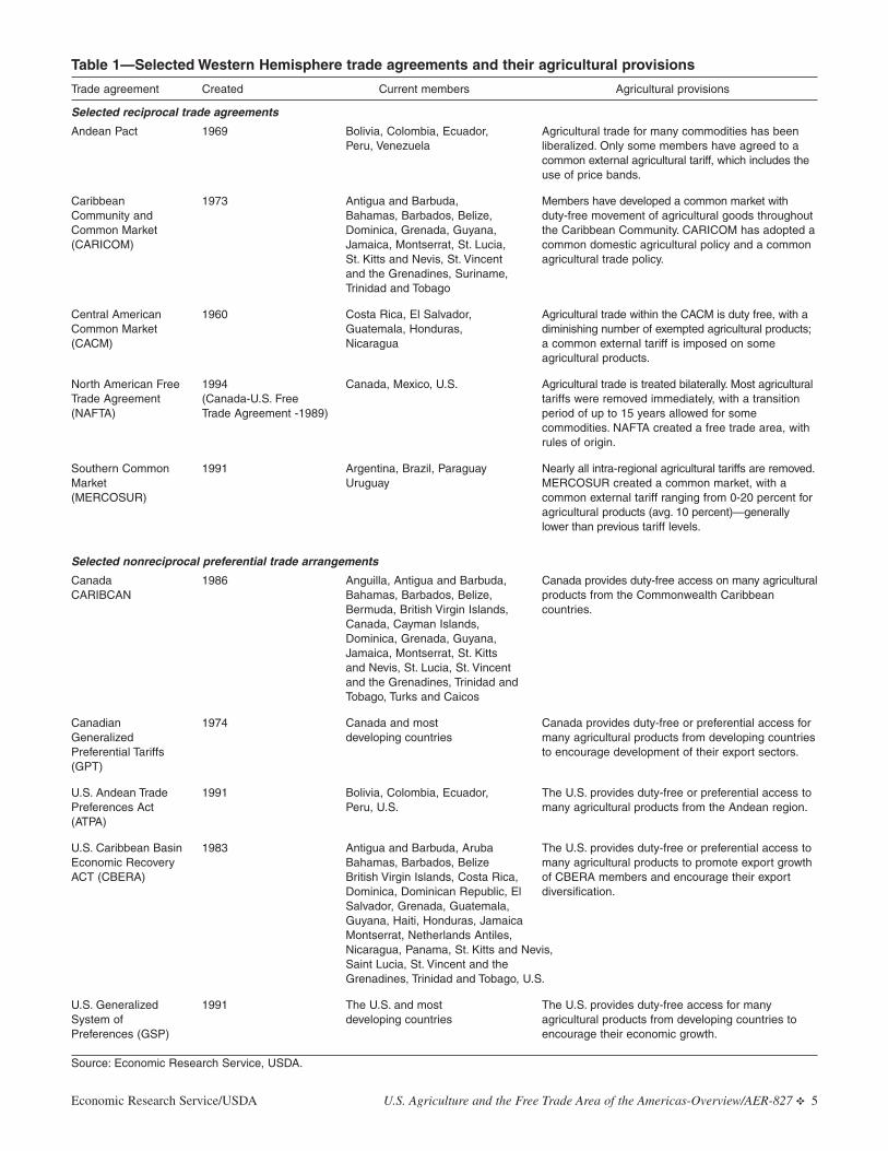
Trade preferences are prevalent in the agricultural trad-ing system in the Western Hemisphere (table 1).Almost every member of the FTAA is now party to atleast one agreement, and the multiple agreements towhich most FTAA members belong create a networkof overlapping memberships within the WesternHemisphere. A role of the FTAA will be to consoli-date, rationalize, and potentially advance the trade lib-eralization that has occurred under these regionalagreements.

Trade Preferences Have Already LoweredAgricultural Tariffs in the Hemisphere

Many types of trade preferences are extended in theWestern Hemisphere. In reciprocal trade arrangements,all parties agree to mutual reduction or elimination oftrade barriers, but the level of market integration canvary. In the Western Hemisphere, the most comprehen-sive reciprocal arrangements are customs unions, whichnow include MERCOSUR, the Central AmericanCommon Market (CACM), and the CaribbeanCommunity and Common Market (CARICOM). In acustoms union, members reduce or eliminate tariffs onproducts of other members and agree on common tar-iffs against the rest of the world. Free trade areas, suchas NAFTA, reduce or eliminate internal tariffs but allowmembers to maintain separate external tariffs. Free tradeareas therefore require detailed rules of origin to preventthe transshipment of imports into the union throughthe country with the lowest external tariffs. The FTAAwill be a free trade area. Other, more limited, types oftrade preferences used in the region include partial scopeagreements, in which trade preferences are given toselected sectors. In economic complementation agree-ments, members increase economic cooperation withthe objective of eventually realizing free trade.

In nonreciprocal preferences, which are applied exten-sively in the Western Hemisphere, only one party pro-vides trade preferences. Among the major nonrecipro-cal arrangements are the U.S. Generalized System ofPreferences (GSP) and Canada’s GeneralizedPreferential Tariffs (GPT), both of which allow duty-free or preferential treatment for many agriculturalimports from developing countries. Generally, neitherarrangement allows preferences for the over-quota tar-iffs of tariff-rate quota (TRQ) regimes. The GSP andGPT preferences apply to all FTAA members, except

NAFTA members, and GSP for Bermuda. Some coun-tries party to GSP and GPT are also eligible for othertrade preferences. The United States and Canada pro-vide nonreciprocal preferences for many agriculturalproducts from the Caribbean area, and the UnitedStates also provides preferences for imports from theAndean countries. Nonreciprocal preferences are con-cessions, not binding commitments; in some cases theymay expire and require reauthorization. Reciprocaltrade agreements that are ratified by their membersprovide a greater degree of assurance about the stabili-ty of negotiated tariff preferences.

In the Western Hemisphere, regional trade agreementsand preferences have largely succeeded in includingagriculture in trade liberalization, although sensitiveimports are often exempted. NAFTA, for example, willeliminate almost all barriers to agricultural tradeamong its members by the time it is fully implementedin 2008, with some exceptions affecting trade withCanada, including dairy, poultry, eggs, peanuts, sugarand sweeteners, cotton, and tobacco. In MERCOSUR,almost all agricultural tariffs are to be removed,although Argentina’s economic crisis has recently ledits government to eliminate regional preferences onmany items, including some food products.

In addition to regional trade agreements with WesternHemisphere partners, many FTAA members have tradeagreements with non-Hemisphere partners. The UnitedStates has free trade agreements with Israel, Jordan, andSingapore. Other negotiations are underway or pro-posed, including agreements with Morocco, the SouthAfrican Customs Union, Bahrain, and Australia.Mexico’s trade agreements include a pact with theEuropean Union (EU) that excludes agricultural com-modities receiving EU domestic support and agreementswith the European Free Trade Association (EFTA) andIsrael. Chile’s agreements include one with the EU,and a MERCOSUR-EU negotiation is in progress.Caribbean countries, along with African and Pacificcountries, are extended preferences from the EU, andHaiti will receive the EU’s “Everything-But-Arms”preferences extended to 48 least developed countries.

Most U.S. Agricultural Imports From the Western Hemisphere Are Already Eligible for Tariff Preferences

Partly due to existing trade preferences, 81 percent($18.8 billion) of U.S. agricultural imports from theregion qualified for duty-free entry in 2001 (table 2).Some of these imports received Most-Favored-Nation



Table 1—Selected Western Hemisphere trade agreements and their agricultural provisions

Trade agreement Created Current members Agricultural provisions

Selected reciprocal trade agreements

Andean Pact 1969 Bolivia, Colombia, Ecuador, Agricultural trade for many commodities has been Peru, Venezuela liberalized. Only some members have agreed to a

common external agricultural tariff, which includes the use of price bands.

Caribbean 1973 Antigua and Barbuda, Members have developed a common market withCommunity and Bahamas, Barbados, Belize, duty-free movement of agricultural goods throughout Common Market Dominica, Grenada, Guyana, the Caribbean Community. CARICOM has adopted a (CARICOM) Jamaica, Montserrat, St. Lucia, common domestic agricultural policy and a common

St. Kitts and Nevis, St. Vincent agricultural trade policy.and the Grenadines, Suriname, Trinidad and Tobago

Central American 1960 Costa Rica, El Salvador, Agricultural trade within the CACM is duty free, with a Common Market Guatemala, Honduras, diminishing number of exempted agricultural products;(CACM) Nicaragua a common external tariff is imposed on some

agricultural products.

North American Free 1994 Canada, Mexico, U.S. Agricultural trade is treated bilaterally. Most agriculturalTrade Agreement (Canada-U.S. Free tariffs were removed immediately, with a transition(NAFTA) Trade Agreement -1989) period of up to 15 years allowed for some

commodities. NAFTA created a free trade area, with rules of origin.

Southern Common 1991 Argentina, Brazil, Paraguay Nearly all intra-regional agricultural tariffs are removed.Market Uruguay MERCOSUR created a common market, with a (MERCOSUR) common external tariff ranging from 0-20 percent for

agricultural products (avg. 10 percent)—generally lower than previous tariff levels.

Selected nonreciprocal preferential trade arrangements

Canada 1986 Anguilla, Antigua and Barbuda, Canada provides duty-free access on many agricultural CARIBCAN Bahamas, Barbados, Belize, products from the Commonwealth Caribbean

Bermuda, British Virgin Islands, countries.Canada, Cayman Islands, Dominica, Grenada, Guyana, Jamaica, Montserrat, St. Kitts and Nevis, St. Lucia, St. Vincent and the Grenadines, Trinidad and Tobago, Turks and Caicos

Canadian 1974 Canada and most Canada provides duty-free or preferential access for Generalized developing countries many agricultural products from developing countries Preferential Tariffs to encourage development of their export sectors.(GPT)

U.S. Andean Trade 1991 Bolivia, Colombia, Ecuador, The U.S. provides duty-free or preferential access to Preferences Act Peru, U.S. many agricultural products from the Andean region.(ATPA)

U.S. Caribbean Basin 1983 Antigua and Barbuda, Aruba The U.S. provides duty-free or preferential access toEconomic Recovery Bahamas, Barbados, Belize many agricultural products to promote export growth ACT (CBERA) British Virgin Islands, Costa Rica, of CBERA members and encourage their export

Dominica, Dominican Republic, El diversification.Salvador, Grenada, Guatemala,Guyana, Haiti, Honduras, JamaicaMontserrat, Netherlands Antiles,Nicaragua, Panama, St. Kitts and Nevis,Saint Lucia, St. Vincent and theGrenadines, Trinidad and Tobago, U.S.

U.S. Generalized 1991 The U.S. and most The U.S. provides duty-free access for many System of developing countries agricultural products from developing countries toPreferences (GSP) encourage their economic growth.

Source: Economic Research Service, USDA.

(MFN) duty-free status accorded by the United Statesto products from WTO member countries. Most ofthese free imports, however, received duty-free treat-ment under NAFTA or other preferences. Trade prefer-ences covered over 60 percent of U.S. agriculturalimports from Western Hemisphere countries in 2001and allowed duty-free treatment or reduced tariff rateson many commodities.

Most of the U.S. agricultural imports that faced dutiesin 2001 entered from NAFTA partners. U.S. tariffs onimports from Mexico will be reduced to zero whenNAFTA is fully implemented in 2008. Some otherdutiable agricultural imports by the United States fromthe region enter under the U.S. TRQ system. In 2001,the U.S. imported $2 billion worth of agricultural com-modities from the Western Hemisphere under its TRQsystem. Of this total, $1.9 billion was under quota, 78percent of which entered duty free, and about$106,000 entered at over-quota tariff rates.

As a result of preferences, average U.S. tariffs on agri-cultural imports from Western Hemisphere countriesare below the average, 2001 U.S. MFN rate of 10.4percent (table 3). Countries qualifying for CBERA orATPA preferences face an average U.S. agriculturaltariff of 1.8 percent, while other FTAA countries, ben-efiting only from GSP, face slightly higher average tar-iff rates. Due to NAFTA, Canada, at 1.2 percent, andMexico, at 0.4 percent, face the lowest average U.S.tariffs among FTAA countries.

In 2001, NAFTA was the only reciprocal trade agree-ment in the Western Hemisphere to which the UnitedStates was a party.3 Therefore, U.S. exports faced

MFN tariffs in all Hemisphere countries other thanCanada and Mexico. The average 2001 bound MFNagricultural tariff of Western Hemisphere countries,excluding the United States, is 43.3 percent. In gener-al, U.S. exports face much lower applied tariffs inthese markets, which average 12.5 percent.4 However,the possibility that countries can increase their tariffsup to rates bound in the WTO creates a degree of riskfor U.S. exporters. Furthermore, U.S. products facethese MFN tariffs while exports from many competingsuppliers in the region have preferential access.

Tariff Protection Remains High on Some Products

While agriculture is included in most preferential tradearrangements in the region, some sensitive productsare allowed exemptions or long transition periods tofree trade (Stout and Ugaz-Pereda). Comprehensivedata on preferential tariffs in the Western Hemisphereare not available, but analysis of applied MFN tariffschedules provides some perspective on which com-modities receive the most protection. Applied tariffrates are generally highest on meats, dairy products,sugar and sugar-containing products, and vegetableoils. Wheat, most oilseeds, fibers, and live plants andanimals have relatively low MFN tariffs. Of interest tothe United States are higher-than-average tariffs ontobacco products, meats, rice, beer, wine, and distilledspirits. Certain fruits and vegetables, including apples,grapes, oranges, grapefruit, potatoes, and onions, alsoface higher-than-average tariffs in many markets, espe-cially during specific times of the year.

Many countries’ agricultural exports are concentratedin a few commodities. For example, in 10 countries inthe Western Hemisphere, a single commodity accountsfor over half of total agricultural exports to the UnitedStates. Due to this commodity concentration, somecountries are more concerned about tariff rates for spe-cific commodities than about overall tariff rates, partic-ularly if products in which they specialize face higher-than-average tariffs. The United States, for example,maintains relatively high tariffs, with limited preferen-tial access, on some agricultural products of specialexport interest to FTAA countries, including sugar,peanuts, tobacco, orange juice, and dairy products.

One way to measure the alignment between an export-ing country’s export concentration and an importingcountry’s tariff peaks is to calculate the weighted average


Table 2—U.S. agricultural imports from theWestern Hemisphere in 2001, by tariff treatment

Import classification Value

$U.S. billion

Total agricultural imports from the Western Hemisphere 23.1Total duty-free imports 18.8

Duty-free imports under MFN (7.5)Duty-free imports under preferences (11.3)

Preferential, nonzero tariffs (NAFTA)1 2.8MFN tariffs less than 5 percent .9 MFN tariffs over 5 percent .6

1All U.S. tariffs under NAFTA will be reduced to zero when theimplementation period is concluded in 2008.

Source: Agricultural Market Access Database.

3In late 2003, the United States entered a bilateral free trade agreementwith Chile. The effects of this agreement on agricultural tariff levels is notincorporated in this analysis.

4These percentages are based on 6-digit aggregates of the HarmonizedSystem. Applied tariff rates are not available for all countries.

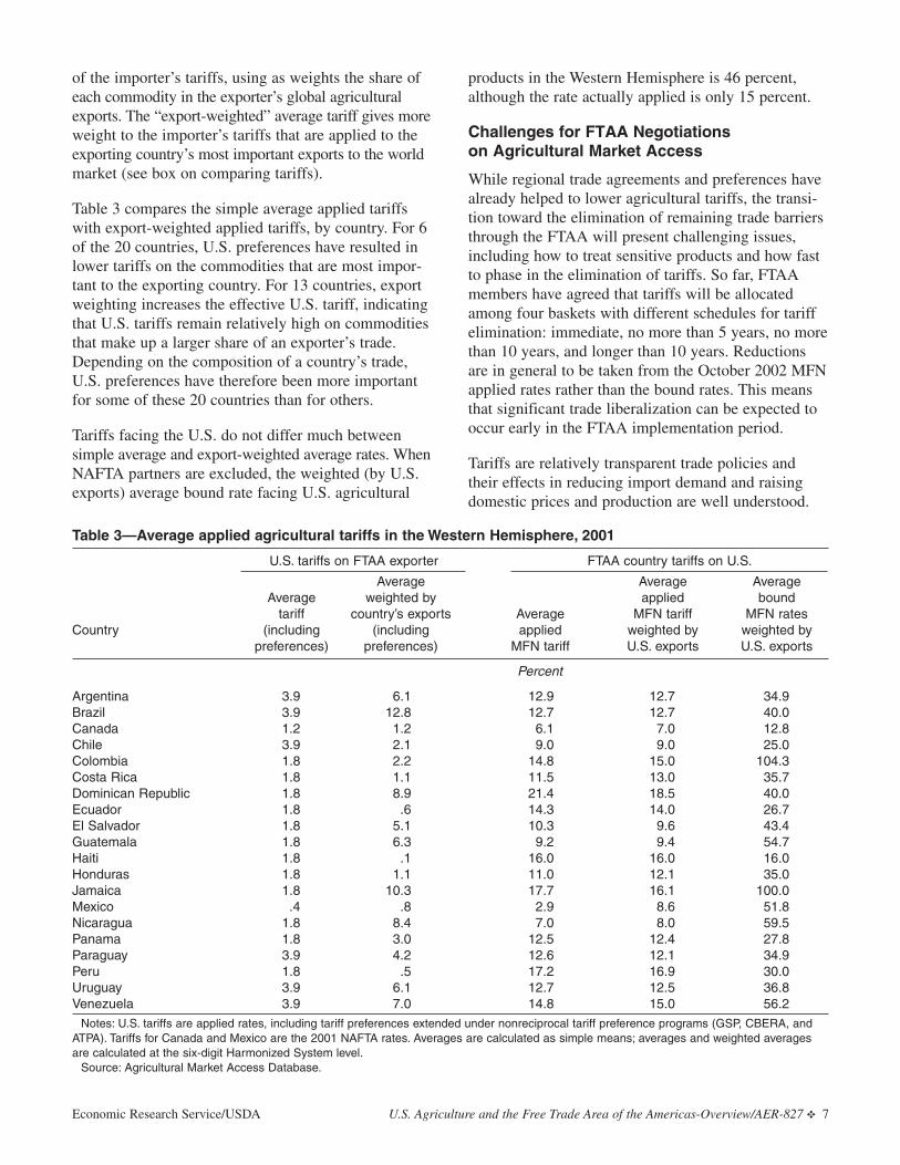
of the importer’s tariffs, using as weights the share ofeach commodity in the exporter’s global agriculturalexports. The “export-weighted” average tariff gives moreweight to the importer’s tariffs that are applied to theexporting country’s most important exports to the worldmarket (see box on comparing tariffs).

Table 3 compares the simple average applied tariffswith export-weighted applied tariffs, by country. For 6of the 20 countries, U.S. preferences have resulted inlower tariffs on the commodities that are most impor-tant to the exporting country. For 13 countries, exportweighting increases the effective U.S. tariff, indicatingthat U.S. tariffs remain relatively high on commoditiesthat make up a larger share of an exporter’s trade.Depending on the composition of a country’s trade,U.S. preferences have therefore been more importantfor some of these 20 countries than for others.

Tariffs facing the U.S. do not differ much betweensimple average and export-weighted average rates. WhenNAFTA partners are excluded, the weighted (by U.S.exports) average bound rate facing U.S. agricultural

products in the Western Hemisphere is 46 percent,although the rate actually applied is only 15 percent.

Challenges for FTAA Negotiations on Agricultural Market Access

While regional trade agreements and preferences havealready helped to lower agricultural tariffs, the transi-tion toward the elimination of remaining trade barriersthrough the FTAA will present challenging issues,including how to treat sensitive products and how fastto phase in the elimination of tariffs. So far, FTAAmembers have agreed that tariffs will be allocatedamong four baskets with different schedules for tariffelimination: immediate, no more than 5 years, no morethan 10 years, and longer than 10 years. Reductionsare in general to be taken from the October 2002 MFNapplied rates rather than the bound rates. This meansthat significant trade liberalization can be expected tooccur early in the FTAA implementation period.

Tariffs are relatively transparent trade policies andtheir effects in reducing import demand and raisingdomestic prices and production are well understood.


Table 3—Average applied agricultural tariffs in the Western Hemisphere, 2001

U.S. tariffs on FTAA exporter FTAA country tariffs on U.S.

Average Average AverageAverage weighted by applied bound

tariff country’s exports Average MFN tariff MFN ratesCountry (including (including applied weighted by weighted by

preferences) preferences) MFN tariff U.S. exports U.S. exports

Percent

Argentina 3.9 6.1 12.9 12.7 34.9Brazil 3.9 12.8 12.7 12.7 40.0Canada 1.2 1.2 6.1 7.0 12.8Chile 3.9 2.1 9.0 9.0 25.0Colombia 1.8 2.2 14.8 15.0 104.3Costa Rica 1.8 1.1 11.5 13.0 35.7Dominican Republic 1.8 8.9 21.4 18.5 40.0Ecuador 1.8 .6 14.3 14.0 26.7El Salvador 1.8 5.1 10.3 9.6 43.4Guatemala 1.8 6.3 9.2 9.4 54.7Haiti 1.8 .1 16.0 16.0 16.0Honduras 1.8 1.1 11.0 12.1 35.0Jamaica 1.8 10.3 17.7 16.1 100.0Mexico .4 .8 2.9 8.6 51.8Nicaragua 1.8 8.4 7.0 8.0 59.5Panama 1.8 3.0 12.5 12.4 27.8Paraguay 3.9 4.2 12.6 12.1 34.9Peru 1.8 .5 17.2 16.9 30.0Uruguay 3.9 6.1 12.7 12.5 36.8Venezuela 3.9 7.0 14.8 15.0 56.2

Notes: U.S. tariffs are applied rates, including tariff preferences extended under nonreciprocal tariff preference programs (GSP, CBERA, andATPA). Tariffs for Canada and Mexico are the 2001 NAFTA rates. Averages are calculated as simple means; averages and weighted averagesare calculated at the six-digit Harmonized System level.

Source: Agricultural Market Access Database.

Many members of the FTAA employ trade barriersthat are more complex, less familiar, and less transpar-ent in their effects on prices and production than tar-iffs. These policies include price bands, seasonal tar-iffs, tariff rate quotas, special safeguards, and domesticabsorption agreements.

One strategy for understanding complex trade policiesis to deconstruct their essential components—theiroperation, their impacts, and their tax burden (whopays)—and compare them with more traditional tariffsand subsidies (table 4). Countries employ many differ-ent types of trade protection and domestic supportpolicies that can have identical effects in raising pricesreceived by producers or in reducing price variability.For example, some countries use price bands to restrictimports when world prices are low, which helps toinsulate and stabilize domestic producer prices.Consumers pay the costs of price bands: they pay tar-iffs on the imported product and face higher prices forthe domestic variety. WTO tariff bindings limit theability of price bands to insulate domestic prices.

In a domestic absorption agreement, prospectiveimporters are first required to purchase a specifiedamount of the product from domestic producers. The

agreement does not change the total amount of the prod-uct consumed in a country, but it does increase theshare of domestic production relative to imports intotal consumption. The increase in demand for thedomestic product leads to higher producer prices,while the amount of imports and tariff revenue collect-ed by the domestic government fall. In effect, a domes-tic absorption agreement leads domestic buyers to shiftexpenditures from the import plus the tariff to theincreased quantity and price of the domestic product.

The FTAA’s mandate includes the identification of trade-distorting practices for agricultural products, includingthose that have an effect equivalent to agricultural exportsubsidies, to bring such policies under greater disci-pline. Some countries argue that agricultural policieswith equivalent producer effects should be disciplinedin the same way, regardless of their implementation.The U.S. position is that multilateral negotiations arethe appropriate forum for addressing domestic supportbecause a country’s production subsidies affect itsglobal, not just its regional, trade. The ongoing WTOmultilateral negotiations are addressing market access,domestic support, and export subsidies.


Comparing Tariffs Across Countries

The aggregation of thousands of individual tariffs into a single, representative measure for each country means that someassumption must be made on how much weight to give individual tariffs. A simple average implies all tariffs are equallyimportant, yet for some countries, most imports may be concentrated in only a few commodities. Giving equal weight totariffs on lightly traded commodities therefore may not be representative of a country’s tariff code. Tariffs are sometimesweighted by the share of each imported commodity in a country’s total imports. But this understates the restrictiveness of acountry’s tariff code because import weights become smaller when tariffs become more restrictive. Consumption weightshave the same measurement bias as import weights. Production weights would assure that highly protected commoditiesproduced in large amounts get appropriately large weights, but production data at the tariff-line level are rarely available.

This report develops export weights in which the importing country’s tariffs are aggregated using as weights the share ofthe commodity in the exporter’s world agricultural exports (Sandrey). An aggregate measure of a country’s tariffs is there-fore calculated for each of its trade partners. This measure gives greater weight to those commodities important to anexporting country and avoids the bias introduced in bilateral trade by the importer’s tariff schedule. It is especially appro-priate when exporting countries are characterized by commodity concentration and the importer’s tariffs are highly distort-ing of that trade. Its limitation is that differences in the composition of its bilateral trade may reflect differences among itspartners’ consumer preferences instead of their tariff structure.

As an example, consider a country for which cinnamon accounts for 95 percent of its global agricultural exports. The exportermay face zero tariffs on all other products in the importer’s market, except for a nearly prohibitive tariff on cinnamon, say100 percent. The importer’s simple average agricultural tariff may be close to zero percent, yet the importer’s single, nearlyprohibitive tariff has a very restrictive effect on its trade with the cinnamon exporter. An import tariff weighted by the shareof the commodity in the exporter’s world trade (95 percent) places a greater weight on the importer’s tariff on cinnamonthan on other products, even if little, or even no, bilateral trade in cinnamon takes place. It will result in a weighted-averagetariff in that importer’s market of close to 95 percent with respect to its cinnamon-exporting partner.

While domestic production subsidies are often difficultto directly negotiate in a free trade area, market forceswould discipline some types of support if free trade isachieved within a region. Open borders can placebudgetary pressure on programs that attempt to sup-port domestic market prices at above free-market lev-els (see box on U.S. sugar in the FTAA). If low-costimports are allowed to enter freely from regional sup-pliers, domestic subsidy costs would have to rise todefend a price support against falling domestic prices.

U.S. Agriculture Has Benefited From TradeLiberalization in the Western Hemisphere

Trends in U.S. agricultural exports during 1980-99, aperiod in which many countries in the WesternHemisphere implemented substantial regional andunilateral trade reforms, provide a valuable perspec-tive on the additional trade benefits that the FTAA islikely to generate. This analysis finds that the trade

reforms already completed in the Western Hemi-sphere have supported an expansion of U.S. agricultural exports to the region.5

The impact of these reforms on U.S. agricultural exportsis most obvious in the case of Mexico, which imple-mented a far-reaching set of unilateral trade reformsbefore it cemented the liberalization of its trade withCanada and the United States by joining NAFTA in1994. In 1999, U.S. agricultural exports to Mexico were2.5 times ($3 billion) higher than they would have beenin the absence of these unilateral and regional tradereforms. NAFTA alone accounted for 20 percent of U.S.


5This analysis is based on a series of “gravity models.” The approach isable to differentiate and measure the impact of trade reforms on U.S.exports to a specific country, compared with other factors, such as the rela-tive closeness of that country’s bilateral trade relationship with the UnitedStates and the size of the importing country’s economy. However, the variables used to identify trade reforms may also capture the influence ofother factors that are contemporaneous to specific trade agreements.

Table 4—Tariffs, complex tariffs, and domestic support: Equivalencies in operation, impacts, and tax burden

PolicyTreatment underWTO disciplines Operation

Impacts onproducer price Who pays?

Ad valorem tariffs Market access Percentage (fixed) tax onimport unit value

Raise domestic producer price Consumers

Specific tariffs Market access Per unit (fixed) tax onimport unit volume


Tariff-rate quotas Market access Low duties applied to with-in-quota volume, highduties applied on over-quota volume


Seasonal tariffs Market access Tax rate dependent onimport season

Raise domestic producer priceduring seasons when productionis highest

Consumers

Special safeguard tariffs Market access Tax rate dependent onimport unit value (pricetrigger) or import volume(volume trigger)

Raise domestic producer priceand reduce its volatility

Consumers

Price bands Market access Tax rate dependent onmarket trends in importunit values and domesticprices


Consumers

Price support Domestic support Fixed producer price floor,subsidy varies withdomestic market price


Government/taxpayers

Domestic absorptionagreements

Trade-related invest-ment measures

Import license and tariffrebate requires purchaseof domestic agriculturalproduct

Raise domestic producer price Consumers/taxpayers(foregone revenue)



U.S. Sugar in the FTAAStephen Haley

Increased FTAA access to the U.S. sugar market is a key issue in the FTAA negotiations on agriculture because U.S.import barriers are high and changes in access will significantly change market conditions facing competing sugar suppli-ers in the Western Hemisphere. The effect of an FTAA on the U.S. sugar industry will depend on how the increase in mar-ket access is achieved and on how U.S. sugar support programs may be modified as a result of these access commitments.

The U.S. domestic sugar market is supported by a sugar TRQ, a nonrecourse loan (price support) program, and a domesticsupply control program (flexible marketing allotments). Excluding NAFTA, the U.S. sugar TRQ system allocates 40 coun-tries the right to export raw sugar to the United States, with quota allocations based on historical trade shares from 1975-81. Twenty-three of the 40 countries are from the Western Hemisphere, and they accounted for 64 percent of the U.S. rawsugar TRQ in 2001. NAFTA currently allows Mexico duty-free access to the U.S. market for a limited quantity of rawsugar. Beginning in 2008, Mexico will have duty-free access with no quantitative limits.

The nonrecourse loan program allows U.S. sugar processors to take out loans from the Government using sugar as collater-al. The loan rate in effect sets a floor price for sugar. After harvest, processors can pay off the loan in cash; alternatively,they can forfeit the sugar to the Government if market prices drop below the loan rate. Sugar forfeitures result in a buildupof Government stocks. The 2002 Farm Security and Rural Investment Act requires the program to be operated at no cost tothe Government. Two mechanisms are used to meet this requirement: allowing processors to purchase sugar fromCommodity Credit Corporation (CCC) stocks in exchange for reduced production, and adjusting marketing allotmentsdownward if imports are below a specified volume.

This case study of sugar analyzes the effects on the U.S. sugar industry of two trade liberalization scenarios: an expansionof the U.S. sugar TRQ (2-million ton, or 280-percent, increase), and an elimination of the TRQ. If the TRQ is expandedbut the current floor price is maintained, increased U.S. imports will likely cause sugar forfeitures to the Government toincrease, with some of the producer adjustment occurring through transfers of publicly owned stocks. It is assumed thatmarketing allotments will be suspended because imports will exceed the threshold. CCC stockholding will become a majorfactor in the adjustment to the FTAA, with stocks projected at 88 percent of the additional market access in 2012.Alternatively, lowering loan rates to levels that would eliminate loan forfeiture by 2010 will allow more adjustmentthrough declining domestic production (see table). While the domestic price will gradually recover to 23 cents, importswill permanently displace some domestic production.

Because the net surplus producer status of the Western Hemisphere is extremely large, and because the largest, lowest costproducers have low transport costs relative to non-Hemisphere competitors, it is assumed that full market access in anFTAA is the equivalent of unrestricted free trade in sugar for the United States. In this scenario, therefore, the U.S. isassumed to eliminate its sugar TRQ and nonrecourse loan program. The implications for U.S. sugar would be significant,with a 61-percent decline in production and a nearly fourfold increase in imports, which would account for almost 70 per-cent of domestic consumption. If the loan rate is abandoned, the U.S. raw sugar price will be closer to the world price, as-sumed to increase to 11 cents per pound. Remaining U.S. producers would face world price movements and constant mar-ket competition with FTAA producers. A large shift from high fructose corn syrup to sugar, while possible, is not likely.

It is not only U.S. producers who will face adjustments to a liberalized U.S. sugar market. Exporters to the U.S. now benefitfrom their access because they are able to sell sugar at the relatively high U.S. domestic price. Some of these exporters arecurrently high-cost producers that will likely have difficulty competing if equal access is provided to all FTAA members.

Adjustment of U.S. sugar to increased market access in an FTAA

Elimination of U.S.2-million metric ton sugar TRQ and

increase in TRQ access loan program

Item Fixed loan rate Reduction in loan rate No loan rate

Loan rate (cents/lb.) 18 13 EliminatedProduction (% change in 2012 from 2008 base) -20.3 -26.6 -61.2U.S. raw sugar price in 2012 (NY - No. 14) 20.2 23.0 13.1Import share of consumption in 2012 38.1 43.6 68.6

Note: The reduction in the loan rate is calculated as the rate that avoids loan forfeiture by 2010.Source: Economic Research Service, USDA.

exports to Mexico during 1994-99. These estimates aresubstantially larger than the assessment of ERS’s 1997NAFTA report (Crawford and Link), which concludedthat U.S. agricultural exports to Mexico in 1996 wereabout 3 percent higher than they would have been inthe absence of NAFTA. The 1997 study, however,which relied upon a computable general equilibriummodel, examined only the first 3 years of NAFTA’s 14-year transition to trade liberalization.

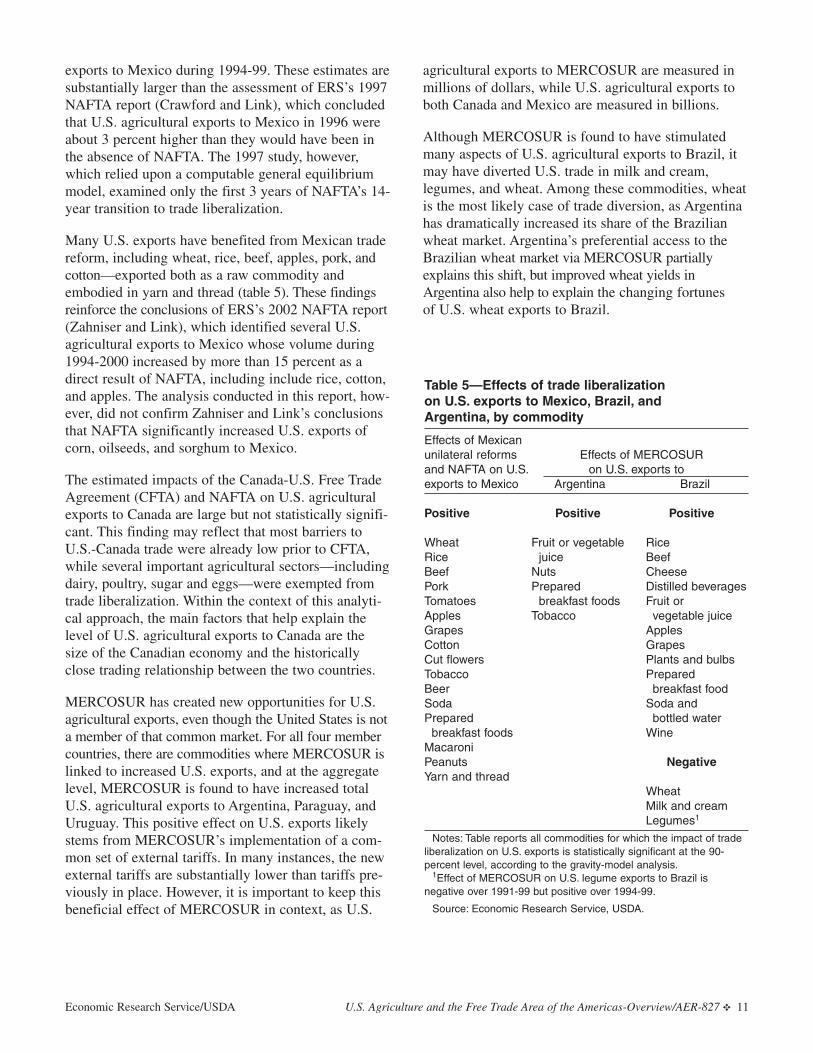
Many U.S. exports have benefited from Mexican tradereform, including wheat, rice, beef, apples, pork, andcotton—exported both as a raw commodity andembodied in yarn and thread (table 5). These findingsreinforce the conclusions of ERS’s 2002 NAFTA report(Zahniser and Link), which identified several U.S.agricultural exports to Mexico whose volume during1994-2000 increased by more than 15 percent as adirect result of NAFTA, including include rice, cotton,and apples. The analysis conducted in this report, how-ever, did not confirm Zahniser and Link’s conclusionsthat NAFTA significantly increased U.S. exports ofcorn, oilseeds, and sorghum to Mexico.

The estimated impacts of the Canada-U.S. Free TradeAgreement (CFTA) and NAFTA on U.S. agriculturalexports to Canada are large but not statistically signifi-cant. This finding may reflect that most barriers toU.S.-Canada trade were already low prior to CFTA,while several important agricultural sectors—includingdairy, poultry, sugar and eggs—were exempted fromtrade liberalization. Within the context of this analyti-cal approach, the main factors that help explain thelevel of U.S. agricultural exports to Canada are thesize of the Canadian economy and the historicallyclose trading relationship between the two countries.

MERCOSUR has created new opportunities for U.S.agricultural exports, even though the United States is nota member of that common market. For all four membercountries, there are commodities where MERCOSUR islinked to increased U.S. exports, and at the aggregatelevel, MERCOSUR is found to have increased totalU.S. agricultural exports to Argentina, Paraguay, andUruguay. This positive effect on U.S. exports likelystems from MERCOSUR’s implementation of a com-mon set of external tariffs. In many instances, the newexternal tariffs are substantially lower than tariffs pre-viously in place. However, it is important to keep thisbeneficial effect of MERCOSUR in context, as U.S.

agricultural exports to MERCOSUR are measured inmillions of dollars, while U.S. agricultural exports toboth Canada and Mexico are measured in billions.

Although MERCOSUR is found to have stimulatedmany aspects of U.S. agricultural exports to Brazil, itmay have diverted U.S. trade in milk and cream,legumes, and wheat. Among these commodities, wheatis the most likely case of trade diversion, as Argentinahas dramatically increased its share of the Brazilianwheat market. Argentina’s preferential access to theBrazilian wheat market via MERCOSUR partiallyexplains this shift, but improved wheat yields inArgentina also help to explain the changing fortunes of U.S. wheat exports to Brazil.


Table 5—Effects of trade liberalization on U.S. exports to Mexico, Brazil, and Argentina, by commodity

Effects of Mexicanunilateral reforms Effects of MERCOSURand NAFTA on U.S. on U.S. exports toexports to Mexico Argentina Brazil

Positive Positive Positive

Wheat Fruit or vegetable RiceRice juice BeefBeef Nuts CheesePork Prepared Distilled beveragesTomatoes breakfast foods Fruit orApples Tobacco vegetable juiceGrapes ApplesCotton GrapesCut flowers Plants and bulbsTobacco PreparedBeer breakfast foodSoda Soda andPrepared bottled water

breakfast foods WineMacaroniPeanuts NegativeYarn and thread

WheatMilk and creamLegumes1

Notes: Table reports all commodities for which the impact of tradeliberalization on U.S. exports is statistically significant at the 90-percent level, according to the gravity-model analysis.

1Effect of MERCOSUR on U.S. legume exports to Brazil is negative over 1991-99 but positive over 1994-99.


Advancing to the FTAA: PotentialEffects on U.S. Agriculture

The FTAA will be a comprehensive agreement that isexpected to address a range of economic issues. Thisanalysis of the expected effects of the FTAA addressesseveral possible negotiating areas with implications forU.S. agriculture, including market access reforms (elimi-nation of agricultural and manufacturing tariffs andother trade measures), foreign direct investment (FDI),U.S. agri-environmental impacts, sanitary and phytosan-itary (SPS) measures, and trade remedy laws (see boxon trade remedy laws).

Welfare Impacts of Market Access Reform in the FTAA

Based on the assumption that all (agricultural and manu-facturing) tariffs will be eliminated, the FTAA willlead to welfare gains (or increased consumer purchas-ing power) of $63 billion for the Western Hemisphere,with gains achieved by every member of the trade agree-ment (table 6).6 U.S. welfare is expected to increase$4.1 billion. Welfare gains derive from two sources:resource reallocation and productivity growth. First,tariff elimination removes tariff-based price distortionsthat influence production and consumption decisions.Countries can then reallocate resources to products inwhich they hold a comparative advantage, and con-sumers can follow their preferences in making expen-diture choices. The resulting allocative efficiency gainsfrom tariff elimination will account for almost $4 bil-lion in welfare gains for the region. Every country willachieve these static welfare gains from the FTAAexcept Chile, which will experience a small loss(under $10 million) due to the welfare costs of itsexport taxes.

Second, the FTAA is expected to generate dynamic gainsin the productive capacity of developing countries in theWestern Hemisphere. The link between trade opennessand accelerated economic growth has been widelyobserved in developing countries and attributed to sever-al sources. Productivity gains accrue when the expansionof exports and imports of capital goods between devel-oping and developed countries leads to technologicalspillovers that stimulate total factor productivity (TFP)growth in the developing countries. These spilloverscan stem from technological advances embodied in

traded goods, “learning by doing,” increased input vari-eties, and the competitive pressures of global markets,all of which help increase the productive efficiency ofland, labor, and capital in all sectors of a developingeconomy. Such potential productivity gains will add $59billion to the estimated welfare impact of the FTAA onthe region, with benefits accruing to every country,including Chile. Welfare gains will be largest inArgentina and Brazil, whose economies will increase insize by about 5 and 7 percent, respectively, due to theFTAA, mainly reflecting the large role of trade in manu-facturing in these economies. By increasing returns tocapital, productivity gains will also help to attract FDI,a goal of the FTAA for the Western Hemisphere’sdeveloping countries but a potential impact that is notincorporated in this analysis.

Aggregate Agricultural Trade Impacts of the FTAA

If all tariffs (agricultural and manufacturing) are elimi-nated in the FTAA and productivity gains are realized,annual agricultural trade within the Western Hemispherewill increase by about $4.0 billion, or about 6 percent(table 7). Agriculture will account for about 20 percentof trade expansion in the Hemisphere due to the FTAA,proportionally larger than its current 9-percent share ofmerchandise trade and a reflection that current agricul-tural tariffs are higher than manufacturing tariffs in manyWestern Hemisphere countries, including the UnitedStates. Annual U.S. agricultural exports to WesternHemisphere countries will increase by $1.4 billion(about 6 percent) due to the FTAA, and U.S. importsfrom the Hemisphere will increase by about $900 mil-


6Welfare, trade, and production effects are based on a simulation using aglobal computable general equilibrium model. These results reflect out-comes after a long-term adjustment (10-15 years) of the world economy totrade liberalization. Results are reported in nominal U.S. 2002 dollars.Percent changes are reported relative to a representative base year (1997).

Table 6—Welfare impacts of an FTAA, by country

Welfare gainsStatic including

welfare productivityCountry gains growth

$U.S. billion

United States 2.3 4.1Canada .1 .2Mexico .1 .3Central America and

the Caribbean .2 4.9Andean countries .5 6.6Argentina .2 20.5Brazil .2 25.3Chile 0 .6Rest of South America 0 .3

Total 3.6 62.8Source: Economic Research Service, USDA.

lion (about 3 percent). The FTAA will be net trade cre-ating in all sectors, including agriculture. In other words,the value of trade that is created within the WesternHemisphere will be greater than the decline in its tradeoutside the Hemisphere caused by preferential tariffs.

FTAA Trade Impacts by Commodity

The largest agricultural trade impacts of the FTAA willbe in processed foods, for which the Western Hemi-sphere’s annual global exports will increase by about$1.5 billion, or 3 percent (table 8). This export categoryis a large, heterogeneous sector that includes fruit andvegetable juices, syrups and confections, frozen seafood,flour, baked goods, roasted coffee and teas, sugar andsugar products, and orange juice. The Western Hemi-sphere’s annual global exports of dairy products will alsohave relatively large growth, at about $330 million, or33 percent, reflecting the high tariffs that remain ondairy products in the Western Hemisphere. The FTAA’sglobal exports of “other crops”—a category that includesfibers, seeds, flowers, and tropical products, such ascoffee and bananas—will increase by about $235 mil-lion, or 3 percent. Global, annual grain exports, includ-ing rice, wheat, and other grains, will increase about$460 million, or 6 percent. The commodity composi-tion of the region’s import growth due to the FTAA issimilar to that of its exports, reflecting that most of thetrade expansion is in intra-regional trade.

Country and Commodity Composition of U.S. Agricultural Trade Growth

The growth in annual U.S. agricultural exports due tothe FTAA will be greatest to Central American andCaribbean countries ($650 million, mostly processedfoods) and Andean countries ($360 million, mostlygrains, and oilseeds and products) (table 9). Annual

U.S. agricultural exports to Canada will increase byabout $160 million (mostly dairy products) becausethe FTAA is assumed to liberalize trade in commodi-ties excluded from NAFTA. Growth in annual U.S.agricultural exports to Argentina ($100 million) andBrazil ($120 million) will be mostly processed foods.

Central America and the Caribbean will also accountfor the largest increase in U.S. agricultural imports dueto the FTAA ($310 million), followed by an increasein imports from the Andean region of $170 million(table 10). Most of the growth in U.S. agriculturalimports from these two regions will be in processedfoods. Although most U.S. tariffs on processed agricul-tural imports from these countries are already zero,U.S. preferences generally maintain high tariffs on asmall number of commodities related to U.S. farmsupport programs, such as chocolate crumb, sweetenedcocoa powders, cake mixes, and other sugar- anddairy-containing products. The United States also has arelatively high MFN tariff on frozen concentrateorange juice, also part of the processed foods sector(see box on U.S. orange juice).

Because trade with the Western Hemisphere accountsfor a small share of U.S. agricultural production, tradeexpansion due to the FTAA will have very smalleffects on U.S. output. Except for rice, real outputwill change less than 1 percent for the aggregate sec-tors described in this report (table 11). Increased U.S.exports will lead to a small expansion of output in


Table 8—Change in annual, global agricultural imports and exports of FTAA members, by commodity

Growth in Growth inFTAA members’ FTAA members’

Commodity global exports global imports

$U.S. million

Rice 179.8 200.7Wheat 130.5 183.1Other grains 146.9 191.9Horticulture 205.0 271.9Oilseeds 126.1 166.7Other crops 234.7 325.7Livestock 45.0 100.9Meats 172.2 265.4Oils and fats 261.0 345.4Dairy products 330.1 350.9Processed foods 1,532.9 1,694.1

Total 3,364.1 4,096.6Source: Economic Research Service, USDA.

Table 7—Change in annual Western Hemisphere and U.S. trade due to the FTAA

Imports Imports Exportsfrom from rest Exports to rest of

Item FTAA of world to FTAA world

$U.S. billionTotal Western

Hemisphere:Agriculture 3.9 0.2 3.9 -0.6Manufacturing 16.2 -3.7 16.2 -1.2

United States:Agriculture 0.9 0.1 1.4 -0.3Manufacturing 6.1 0.7 6.5 -2.6Source: Economic Research Service, USDA.


oilseeds, oils and fats, milk, and dairy products. U.S.sugar production could decline significantly, depend-ing on how the domestic support program may bemodified in response to increased sugar imports fromthe Western Hemisphere countries (see box on U.S.sugar). The moderate decline in U.S. orange juice pro-duction due to the FTAA will be reduced if growthcontinues in U.S. demand for domestic, not-from-con-centrate orange juice (see box on U.S. orange juice).

Inclusion of United States, Agriculture, Maximize Benefits of the FTAA

U.S. participation in the FTAA will help the WesternHemisphere attain the full potential benefits of theagreement. The large size of the U.S. economy makesit the single most important market for the rest of theregion. In agriculture, U.S. participation will account

for about one-third of the region’s global agriculturalexport growth due to the FTAA and about one-quarterof the region’s global agricultural import growth (table12). For U.S. trade partners, the potential trade oppor-tunities with the United States will support both theirefficiency gains based on increased trade and special-ization, and potential productivity gains linked to theexpansion of trade between developing and developedcountry partners. For the United States, participation inthe FTAA ensures expansion of both U.S. agriculturalexports and imports. Without U.S. participation, U.S.agricultural exports would decline because preferentialtreatment will be extended to competing supplierswithin the region through the terms of the agreement.Also, U.S. agricultural import growth, which lowersfood costs and increases variety for consumers, wouldbe diminished.

Table 9—Change in U.S. agricultural exports due to the FTAA

Central Rest ofAmerica and Andean South Total Rest of

Commodity Canada Mexico Caribbean countries Argentina Brazil Chile America FTAA world World

$U.S. million

Rice 0 -2 102 12 0 0 0 0 112 -14 98Wheat 0 2 22 45 0 0 0 1 70 -11 59Other grains -8 -27 56 60 12 1 3 0 98 -7 91Horticulture -7 1 34 22 3 10 1 0 65 -30 35Oilseeds 1 -9 14 29 32 30 1 0 98 -21 77Other crops -3 0 66 32 13 21 1 0 129 -39 90Livestock -3 -2 19 4 4 3 1 0 26 -33 -7Meat -8 -1 77 25 2 4 0 2 102 -52 50Oils and fats 0 -3 64 67 1 3 2 1 135 -10 125Dairy products 203 -2 25 10 2 3 0 1 242 -10 232Processed foods -16 1 171 57 34 45 8 25 325 -110 215Total agriculture 159 -43 649 363 104 121 18 31 1,401 -336 1,065


Table 10—Change in U.S. agricultural imports due to the FTAA

Central Rest ofAmerica and Andean South Total Rest of

Commodity Canada Mexico Caribbean countries Argentina Brazil Chile America FTAA world World

$U.S. million

Rice, raw 0 0 0 0 0 0 0 0 0 8 8Wheat 1 0 0 0 0 0 0 0 1 0 1Other grains 34 0 0 0 1 0 3 0 38 4 43Horticulture 0 5 14 1 1 10 22 0 54 1 55Oilseeds 0 0 1 0 0 3 0 0 4 0 4Other crops 1 3 15 5 1 24 2 0 53 2 55Livestock 27 3 0 0 1 1 0 0 33 13 46Meat 9 0 1 0 0 2 0 1 13 9 22Oils and fats 3 0 0 0 0 1 0 0 4 4 9Dairy products 0 0 1 0 4 0 0 1 7 7 13Processed foods 10 3 279 164 47 91 75 10 679 39 718Total agriculture 86 15 311 171 56 133 102 12 886 88 974


Agriculture is often a sensitive sector in free tradeagreements because most countries provide domesticsupport or relatively high trade protection to their agri-cultural producers, and the effectiveness of some ofthese policies could be compromised by freer trade.Reflecting the diverse levels of economic developmentof FTAA members, their agricultural policies evidencea range of objectives, including providing farm incomesupport, reducing price or income variability, provid-ing income and employment in rural or low-incomeareas, and stimulating economic development. Whilethe use of agricultural support and protection createchallenges for the inclusion of agriculture in theFTAA, benefits will be greater if agriculture is includ-ed, rather than excluded, in the agreement. Trade liber-alization of manufacturing alone would increase FTAAmembers’ demand for manufacturing imports, causingsome countries to reduce their agricultural productionand trade to shift resources into industry. This redistri-bution of agricultural to manufacturing production willlead to a small increase in demand for agriculturalimports in these countries. In addition, productivitygains linked to expanded trade in manufacturing sec-tors will stimulate consumer demand for all products,including food. The effects of the FTAA on agricultur-al trade in the Western Hemisphere will therefore stillbe positive but far smaller if agriculture is excludedfrom trade reform. Including agriculture in the FTAAincreases these positive effects through the potentialefficiency and welfare benefits linked directly to agri-cultural trade liberalization.

Foreign Direct Investment in Processed Foods: FTAA Could Expand Existing Agreements

Over the past decade, foreign direct investment (FDI)in the processed food industries has increased its rolein the Western Hemisphere’s agricultural economy. In2001, the stock of U.S. FDI in the region’s processedfoods industries was about $13 billion, more than dou-ble the level in 1990 (fig. 1). These investments gener-ated $45 billion in sales of processed foods in 2000,also doubling in value since 1990 (fig. 2). These salesin 2000 exceeded the value of U.S. exports to theregion of processed foods in 2000 ($12.5 billion).

Most U.S. FDI in the Western Hemisphere is inMexico and Canada, where both trade and investmentin processed foods have steadily increased. Some ofthe increased trade in processed products, especiallybetween the United States and Canada, is linked togrowth in FDI. The two countries trade many semi-processed food items that are made into highlyprocessed foods by U.S. affiliates serving both U.S.and Canadian markets.

Brazil and Argentina are also major host countries forU.S. FDI. Two factors make FDI more efficient thantrade as a means for U.S. entry in these countries’processed foods markets. First, the two countries aresimilar to the United States in types of crops produced,which makes them competitors in the supply of inputsto the food industry. Second, the high transport costsbetween the Northern and Southern Hemispheres gen-erally make it more cost efficient to purchase agricul-tural inputs locally than to import them.


Table 11—Effects of the FTAA on U.S.agricultural production, by sector

Real changeCommodity in output

Percent

Rice 3.2Wheat 0.0Other grains -0.5Horticulture 0.0Oilseeds 0.4Other crops -0.6Livestock -0.4Milk (raw) 0.1Meat -0.3Oils and fats 0.5Dairy products 0.1Processed foods -0.1


Table 12—Change in annual global agricultural trade due to the FTAA, without U.S. participation and without agriculture

Rest ofWestern

United States Hemisphere

Item Exports Imports Exports Imports

$U.S. billionFTAA, including

U.S. and agriculture 1.07 0.97 2.30 3.12

FTAA without United States -.01 .06 1.47 1.39

FTAA without agriculture -.05 .12 .06 .60Source: Economic Research Service, USDA.


The United States is not the only foreign investor inthese four markets, but it accounts for significantshares of FDI in their food industries (table 13).Country shares of FDI change continually, mainlybased on the underlying “profit and loss” of individualfirms. Shares are unlikely to reflect preferentialinvestor treatment or “investment diversion” becauseof the fundamental change in the climate for FDI inthe Western Hemisphere over the past decade. Latin

American countries underwent a widespread adoptionof investment treaties during the 1990s, in an effort toattract needed foreign capital (OAS). These treatiestypically grant national treatment to foreign investors,eliminate most restrictions on capital and profit remit-tances, and specify dispute settlement procedures.

Most countries in the Western Hemisphere are nowparty to at least one bilateral investment treaty. TheUnited States is party to bilateral investment treatieswith 10 Western Hemisphere countries, includingArgentina. Some regional trade pacts also affordinvestment protection. The NAFTA agreement guaran-tees its members national treatment of investment andspecifies a dispute settlement process. MERCOSURhas investment treaties governing both members andnonmembers, including the United States.

In the FTAA, FDI is being addressed in the negotiatinggroup on investment. The objectives of the negotiationsare to establish a fair and transparent legal frameworkand to create a stable and predictable environment thatprotects the investor, without creating obstacles toinvestment from outside the Western Hemisphere. Sofar, FTAA members are in general agreement on thetypes of protection to be addressed in the pact, includ-ing expropriation and compensation, transparency oflaws, and dispute settlement, and members agree notto relax labor and environmental laws to attract invest-ment. Members have yet to determine whether theseprotections will be extended to new investment or berestricted to existing investment, and whether the pactwill cover financial portfolio investments as well asreal, direct investments (U.S. GAO).

Incorporating investment protections in the FTAA wouldlock in the benefits already provided to the UnitedStates by bilateral and regional treaties, and it wouldextend protection of U.S. investments to the remainingcountries in the Western Hemisphere with which itdoes not have treaties. These investment protectionscould expand the potential market for U.S. FDI in

Figure 1

U.S. FDI position in the Western Hemisphere processed food industry during 1990-2001

$U.S. billion

1990 92 94 96 98 2000

16

14

12

10

8

6

4

2

0Other

Canada

Mexico

BrazilArgentina

Source: Economic Research Service, USDA. Calculations based on data from the Bureau of Economic Analysis.

Figure 2

U.S. FDI generates $45 billion in food product sales in the Western Hemisphere

$U.S. billion

1985 87 89 91 93 95 97 990

5

10

15

20

25

30

35

40

45

50

Other

Canada

Mexico

BrazilArgentina

Source: Economic Research Service, USDA. Calculations based on data from the Bureau of Economic Analysis.

Table 13—U.S. share in total FDI in processed food industries, 2000

Country U.S. share in FDI

Percent

Argentina 25Brazil 40Canada Over 50Mexico 60Source: Economic Research Service, USDA. Calculations based ondata from the Bureau of Economic Analysis and UNCTAD.


Trade Remedy Laws in the FTAA John Wainio

FTAA countries are discussing trade remedy laws, which are used to counter imports that have been allegedly dumped byfirms in the exporting country or subsidized by the government of the exporting country. National trade remedy laws are aparticularly contentious issue, as some countries believe trade remedy laws are a form of thinly veiled protectionism. Othercountries, including the United States, see these laws as essential to efforts to liberalize trade. Without them, they argue, itwould be hard to assure domestic industries that they would be protected against unfair trade practices by other countries.

The initial proposals tabled within the Subsidies, Antidumping, and Countervailing Duties Negotiating Group of the FTAdiffered extensively. At one end of the spectrum, the United States argued that countries should be allowed to maintain theircurrent trade remedy laws; at the other end, some proposed that use of trade remedy laws be limited or even eliminatedwithin the FTAA (U.S. GAO). While negotiators have made progress in certain areas, a number of issues remain unresolved.Chief among these is the extent to which the FTAA will modify WTO rules to tighten the requirements that must be metbefore an FTAA country can impose antidumping and countervailing duties on other countries within the region. The UnitedStates is concerned that this could create a body of law that would be divergent from U.S. law applied to countries that arenot members of the FTAA. This could complicate antidumping investigations that target suppliers from multiple countries,both within and outside the Western Hemisphere, as well as pose legal implications within the WTO.

In 2001, 10 FTAA countries reported having 634 active trade remedy measures in place (see table). Fourteen FTAA coun-tries were the targets of these measures. The majority of these measures, 569, or 90 percent, were the result of allegeddumping. Five countries were applying both antidumping (AD) and countervailing duties (CVD), and five had onlyantidumping duties.1 Eighteen percent of the antidumping measures applied by FTAA countries and 14 percent of thecountervailing measures were assessed against imports from countries within the Western Hemisphere. The United Stateswas the only country applying countervailing duties against its regional trading partners. The United States was also theheaviest overall user of trade remedy measures within the Western Hemisphere, with 32 measures in place against otherFTAA countries. This represented 10 percent of U.S. AD/CVD measures in place on December 31, 2001.

The United States was also the main target of other countries’ measures within the region, with 39 antidumping measuresin place against U.S. exports. The United States had measures against imports from five countries in the region (Argentina,Brazil, Canada, Chile, and Mexico), while six countries had at least one measure in place against the United States(Argentina, Brazil, Canada, Colombia, Mexico, and Venezuela).

1Another three countries (Chile, Costa Rica, and Uruguay) have reported trade remedy investigations in the past, but none reported active measure inplace to the WTO during 2001.

Number of final antidumping and countervailing duty measures in force within the FTAA,as of December 31, 2001

Countries applying both antidumping (AD) Countries applying only Totaland countervailing duties (CVD) antidumping duties FTAA

TrinidadUnited andStates Argentina Canada Mexico Venezuela1 Brazil Colombia Jamaica Peru1 Tobago1 AD CVD

Exporting country AD CVD AD CVD AD CVD AD CVD AD CVD AD AD AD AD AD

NumberArgentina 6 2 1 1 8 2Brazil 1 4 11 5 3 20 4Canada 6 2 6 2Chile 2 3 2 2 9 0Colombia 0 0Costa Rica 0 0Guatemala 0 0Jamaica 0 0Mexico 8 1 2 1 3 2 16 1Nicaragua 0 0Trinidad and Tobago 1 1 0United States 1 14 11 2 5 3 36 0Uruguay 1 1 0Venezuela 1 1 1 3 0

FTAA total 23 9 17 0 21 0 15 0 2 0 13 4 0 4 1 100 9Global total 260 48 47 3 94 10 61 1 19 3 53 14 1 15 5 569 65FTAA share of

global (%) 9 19 36 0 22 0 25 0 11 0 25 29 0 27 20 18 141Measures for Peru, Trinidad and Tobago, and Venezuela are as of June 30, 2001.Source: WTO members’ semi-annual reports to the Committees on Anti-dumping practices and Subsidies and Countervailing measures.


An Analysis of the U.S. Orange IndustryJason Donovan* and Barry Krissoff

*Donovan is a USDA agricultural economist at the Center for Tropical Agricultural Research and Higher Learning (CATIE), Turrialba, Costa Rica.

The U.S. orange juice industry receives considerable tariff protection from imports. Given this insulation, U.S. juice pro-ducers and orange growers are concerned that the FTAA’s reduction or elimination of the U.S. tariff on orange juice con-centrate will expose the domestic sector to low-priced imports from the world’s largest orange juice exporter, Brazil. Asimports increase, U.S. processors are likely to demand fewer oranges from domestic growers. Currently, juice processorspurchase 95 percent of Florida fresh orange production.

Our analysis of the U.S. orange and juice industry uses a global model of the orange juice sector. The model accounts forboth the full implementation of NAFTA and the recent, and increasing, preference of U.S. consumers for not-from-concen-trate (NFC) relative to frozen concentrate orange juice (FCOJ). If U.S. consumer preferences remain unchanged, elimina-tion of the U.S. tariff on orange juice concentrate will lead to a substantial (26 percent) increase in orange juice imports by the United States, mostly of FCOJ (see table). Under this scenario, imports from Brazil will increase by 55 percent.Imports from other suppliers, however, will decline. Production of U.S. oranges will decline by 3 percent and U.S. prices will drop 15 percent. Grower revenue would fall 17 percent.

Our analysis also distinguishes between the two prevalent types of orange juice consumed, FCOJ and NFC. Consumersconsider NFC orange juice to be of higher quality than FCOJ and are willing to pay a premium for it. The share of NFC inU.S. orange juice consumption has increased from 15 to 40 percent over the last 10 years. The high cost of transportingNFC juice from Brazil to the U.S. gives domestic producers a comparative advantage in supplying this product, althoughinnovations in transportation technology could make imports more competitive in the future. Changes in U.S. consumerdemand for orange juice and in transportation technologies are therefore key variables that could determine the effect ofthe FTAA on the U.S. orange and orange juice industry.

If the trend in increased consumer preference for NFC orange juice continues, even at a fairly small rate, overall U.S.orange juice production will experience a more modest decline, with less of an impact on the derived demand for U.S.-grown oranges. The potential shift in consumer preferences to NFC, combined with the FTAA, would result in decreases of2 percent in domestic orange production and 4 percent in domestic prices. Grower revenue would drop 6 percent.

Effects of the FTAA on the U.S. orange and orange juice industries

Change with FTAA plus:Continued

Base period No changes increase inU.S. industry quantity in U.S. U.S. preferencesegment or price preferences for NFC1

Million gal SSE -----------Percent-----------Orange juice imports 376 26.1 23.4

Frozen 369 26.6 23.7NFC 7 3.4 15.0

Orange juice production 1,370 -2.7 -1.9Frozen 753 -4.9 -8.2NFC 617 -0.1 5.6

Dollars/gal SSEFrozen juice price 1.32 -10.4 -10.1NFC price 1.82 -5.6 3.6

MillionsOrange boxes 217 -2.7 -1.9

Dollars/boxOn-tree orange price 5.01 -15.1 -3.8

Notes: Juice yield conversion factor is 6.3 SSE gallons per box. NFC = Not from concentrate. SSE = Singlestrength equivalent. Base period is a simulation of post-NAFTA implementation quantities and prices.

1Scenario assumes a 2.5-percent increase in NFC share of consumption.Source: Economic Research Service, USDA.

processed foods. However, FDI is influenced by manyfactors in addition to investment protection, particular-ly prospects for economic growth, a favorable businessclimate, and economic and political stability. Theseeconomic and political determinants of FDI are likelyto be positively influenced by regional integration inthe FTAA and may have a greater effect on stimulatingfurther growth in FDI than any additional investmentprotection provided by the FTAA agreement.

Potential Agri-Environmental Impact of the FTAA

Within the past decade, environmental and consumergroups have called for formal consideration of theenvironmental impacts of trade agreements. One con-cern of these groups and others is that some countriesmay respond to expanded export opportunities byweakening their environmental standards to lowercosts of production and attract foreign investment.Firms will then relocate production facilities to the lessregulated country, resulting in a loss of jobs at homeand a worsening of pollution as more productionoccurs using dirty technologies. The prevention ofsuch a scenario in free trade is being primarilyaddressed in the FTAA’s investment negotiations. The draft text includes a proposal that labor and environmental standards may not be weakened toattract foreign investment.

Weak environmental standards that already exist in somedeveloping countries are another cause for concern.Compliance with environmental regulations in devel-oped countries is assumed to impose costs, creatingunfair competition if trade is liberalized between countries with different environmental standards.Differences in per capita incomes and levels of devel-opment are a reason that some countries have lowerenvironmental standards than others. Environmentalstandards are more likely to be weak in low-incomecountries, although the income level itself may not bethe driving factor (Dasgupta et al.). Conditions associ-ated with countries that have lower income levels, suchas weak regulatory environments and limited access toinformation on the costs of environmental damage,also lead to poor environmental quality.

Some argue that an improved environment is anachievable goal for the long run, as the economicgrowth associated with trade liberalization will lead tohigher incomes and higher environmental standards indeveloping countries. Whether pollution could or mustincrease during the developmental transition has beena key issue in the debate on trade and the environment.

A growing body of empirical evidence on the relation-ship between income levels and the environment sug-gests that developing countries today are better able toimprove their environmental quality at lower levels ofincome and earlier stages of development than histori-cally (Dasgupta et al.). Factors influencing this changeinclude greater levels of public concern and greaterknowledge about the costs of pollution. Trade liberal-ization, too, has been an influence; in addition to stim-ulating income growth, it allows the speedier adoptionof newer and cleaner technologies and efficiency gainsthat typically are based on production practices thatare less polluting.

To address growing concerns about the effects of globalization on the environment, the United Statesdeclared in 2001 that all trade agreements in which itwill take part will be subject to an assessment of eachagreement’s impacts on the U.S. environment.Determining how such reviews are to be conductedand the scope of potential impacts that should or canbe considered is a challenge for researchers and regu-lators. While research is available to support impactanalyses of some indicators of conventional pollutants,many other pollutants are untested and still others maybe unknown but of potentially great concern in thefuture. Environmental impact evaluations must there-fore remain a sufficiently flexible process to adapt tochanges in technologies, the level of knowledge aboutthe environment, and social concerns about, anddemand for, environmental quality.

The FTAA will be subject to an environmental review.Because trade liberalization in the FTAA is expectedto have minimal effects on U.S. agricultural produc-tion, it has only a small potential to affect the U.S.agri-environment, and these impacts can be assessed inan agriculture sector model. The analysis reported hereis not an official environmental review. It providesanalysis of some of the agri-environmental indicatorsthat could be included in such reviews.

Measurable environmental indicators for agricultureinclude soil depreciation, nitrogen loss, and soil ero-sion as production scale, composition, technologies,and location change.7 The relatively small effects ofthe FTAA on U.S. agricultural production will result inonly small impacts on these agri-environmental indica-tors. The FTAA will yield small benefits in terms ofsoil erosion and water pollution from nitrogen and


7The analysis in this section draws on the U.S. Mathematical ProgrammingModel (USMP), a spatial and regional partial equilibrium model describedin House et al. (1999).

phosphorus, with reductions of less than 0.2 percent ofbaseline values. It will, however, result in small envi-ronmental costs in terms of air pollution from nitrogenand soil depreciation, with increases of less than 0.1percent of baseline values. The environmental impactsof the FTAA cannot yet be measured for sugar, amongother products. Studies of sugarcane production inFlorida suggest that a decrease in U.S. productioncould improve environmental quality as water-reten-tion capacity in the neighboring Florida Evergladeswatershed increases. However, the final environmentalconsequence of retiring sugar acreage will depend onalternative uses of that land.

Sanitary and Phytosanitary Issues in the FTAA: Challenges of Implementation

Sanitary and phytosanitary measures can pose signifi-cant barriers to trade, and they are likely to becomemore prominent as tariff barriers are lowered. FTAAmembers have therefore committed themselves toidentifying and developing mechanisms needed tofacilitate Western Hemisphere trade consistent with theWTO SPS agreement concluded in the UruguayRound and implemented in 1995. The WTO agreementprovides a set of multilateral rules that ensure SPSmeasures are applied only to achieve appropriate levelsof protection for human, animal, or plant life or health.To ensure that such regulations are not protection poli-cies “in disguise,” the agreement requires them to bebased on scientific principles.

Negotiation of an agreement on SPS measures in theFTAA is expected to address whether the WTO SPSagreement provides a sufficient framework for theregional trade pact, or whether the region should pur-sue a “WTO-plus” agreement that spells out additionalrights and obligations. So far, debate on SPS matters inthe FTAA has mainly been over the implementation ofcurrent WTO SPS obligations in the region, rather thanthe WTO agreement’s fundamental principles. Ad-vancing to a WTO-plus agreement presents challenges:it is difficult to draft prescriptive rules to bring about amore energetic fulfillment of current obligations with-out codifying procedures that could become increas-ingly inappropriate as technology, institutions, and theWTO SPS agreement itself change over time.

The key issues on SPS in the FTAA are likely to mir-ror those in the WTO—particularly the concerns ofdeveloping country exporters about their ability tomeet the increasing demand for food safety in devel-oped countries. Developing country exporters need

constructive solutions and assistance in fulfilling theirobligations and in exercising their rights under theWTO SPS agreement.

Some countries have offered proposals that addressimplementation of the core principles of the WTOagreement: transparency, science-based standards,equivalence, regionalization, and multilateral harmo-nization. Transparency requires that countries notifythe WTO (and, therefore, all trade partners) of changesin SPS regulations. Countries can also counter-notify,or complain, about other countries’ regulations.Increased regulatory transparency in the region couldimprove the functioning of markets. While the majoreconomies in the Western Hemisphere, including theUnited States, Canada, Mexico, Argentina, Brazil, andChile, routinely notify the WTO of their proposed reg-ulations, about one-third of Western Hemisphere coun-tries (primarily the Caribbean countries) have not sub-mitted any notifications to the WTO. Many developingcountries have requested assistance with procedures,including translation of documents and extensions ofdeadlines.

Countries must be able to reference scientific evidenceto support their risk mitigation measures. Developedcountry exporters have the resources to successfullychallenge the scientific rationale of others’ measures, aswell as employ new, scientifically based initiatives toensure food safety. For many of the smaller economies,the resources needed to establish a scientific basis forregulations are limited. Weak science is one factor thatmakes the equivalence principle difficult to implementbetween developed and developing countries. Theequivalence principle ensures the right of exportingcountries to use different measures if they demonstra-bly achieve the same safety outcome as importers’ reg-ulations, but insuffient inspection and services indeveloping countries often preclude them from takingadvantage of this provision. This problem is increasingbecause a growing number of SPS measures areprocess standards designed to check the potential forhazards at critical points during production, rather thanproduct standards that address the testable characteris-tics of the finished product only.

Regionalization, which allows trade among regions ofcountries where the risk of disease and pest transmissionis low, was incorporated into NAFTA as well as theWTO SPS agreement. Regionalization is already open-ing trade in the Western Hemisphere. Chile is allowingimports of fresh melons and watermelons from someparts of the United States. The United States is allow-


ing avocado imports from specified regions of Mexicoto the Northeast and Midwest, and is consideringopening access to all 50 States. In general, however,the benefits from regionalization have been con-strained in many developing countries in part becauseregionalization requires adequate public investment inlaboratory, inspection, monitoring, and certificationinfrastructure.

Like domestic support policies, SPS measures insome respects cannot be effectively addressed in aregional framework. SPS rules cannot be tailored forspecific products of interest nor can preferential rulesand regulations be established for regional partners.

Technical assistance, however, can be targeted region-ally and may be especially suitable for the coalition ofdeveloped and developing countries that form theFTAA membership. Experience with the WTO SPSagreement suggests that technical assistance is aneffective mechanism for addressing barriers to tradeand helping to improve food safety. Options for techni-cal assistance within the FTAA include assistance inpest and disease eradication, strengthening of publicsector testing and certification capacity to speedequivalence determinations and support regionaliza-tion, and support for greater participation of develop-ing countries in the activities of international standard-setting institutions.


The FTAA and the Doha Development Agenda

FTAA members (except the Bahamas) are negotiatingtheir regional trade agreement at the same time thatthey are engaged in multilateral negotiations in theWTO Doha Development Agenda. Globally, the con-tinued proliferation of regional trade agreements indi-cates that regionalism and multilateralism havebecome accepted as dual trade strategies for mostcountries. As of June 2003, 140 regional trade agree-ments are in force. Nearly every country in the worldis now a member of at least one trade agreement(Crawford and Laird). Nevertheless, the benefits of a regional versus a multilateral trade strategy is thesubject of a continuing public policy debate (Burfisherand Zahniser).

Multilateralism will always be a “first best” strategybecause it is nondiscriminatory, that is, all countriesparticipate and offer similar tariff treatment to allWTO members. This principle of nondiscriminationforms the foundation of today’s global trade rules.Regionalism, on the other hand, violates this principleby offering preferential tariff treatment to selectedtrade partners. Opponents of regionalism argue that thecreation of trade among a small group of preferredtrade partners is mostly achieved at the expense oftrade with and investment in nonmembers, and it may create large blocs of countries with competingregulatory and instititutional practices.

Advocates of regionalism generally emphasize itsincremental and more attainable benefits, comparedwith global reform. Regional agreements are morelikely to achieve deeper and faster reform among like-minded partners than is possible in the more diversemultilateral negotiations. Advocates also argue that aregion’s successful experience in dealing with nontariffbarriers following the removal or reduction of regionaltariffs can provide experience that strengthens the mul-tilateral process. The newer regional agreementsformed in the past decade, particularly those in theWestern Hemisphere, have also helped to accelerateeconomic growth in small economies by locking inunilateral reforms, stimulating investment and produc-tivity growth, and fostering links with large and moredeveloped economies (Ethier). For small, reformingcountries especially, regionalism can play a role as afirst step in engaging in the global trading system, andit helps give such countries a greater stake in a rules-based global trading system. Trade rules that ensurepredictability and fairness in trade relationships, and

that offer a credible enforcement mechanism, provideconditions that are favorable for the conduct of busi-ness, investment, and the expansion of trade.

As the Western Hemisphere pursues a regional agree-ment, two factors make multilateral agricultural reformof continued importance for FTAA members. First,FTAA countries are global agricultural traders. Theydepend on non-FTAA markets, with about 65 percentof their agricultural exports destined for, and 35 per-cent of their agricultural imports originating from, out-side the Western Hemisphere. Non-FTAA markets areespecially important for the United States and Brazil,for whom they account for 75-80 percent of total agri-cultural exports. The FTAA region is also a majortrade bloc in global agricultural markets. Agriculturalexports going outside the Western Hemisphere accountfor about 45 percent of world agricultural trade, andimports from the rest of the world account for about 9percent of that trade.

The Western Hemisphere’s position as a large net agri-cultural exporter gives it a great stake in WTO negotia-tions that may further liberalize global agriculturalmarkets. Despite the reforms achieved in the UruguayRound, these markets are still characterized by signifi-cant policy distortions (USDA). Further multilateralreform will impose disciplines on FTAA members andthe rest of the world alike. However, in general, the levelof distorting policies used by FTAA members is lowerthan in most other countries and regions. The average,post-Uruguay Round bound agricultural tariff of FTAAcountries of about 40 percent is lower than the globalaverage bound rate of 62 percent (Gibson et al.). Theaverage applied rate of FTAA countries is about 13 per-cent. Domestic support in the FTAA is also relativelylow. The 2002 producer support estimates for the threeFTAA members of the OECD are 18 percent (UnitedStates), 20 percent (Canada), and 22 percent (Mexico)—below the aggregate OECD rate of 31 percent (OECD).Finally, export subsidies by FTAA members are mini-mal, with the EU accounting for over 90 percent of global expenditures on these subsidies in 1998 (Leetma).

These patterns in agricultural trade flows and agriculturalpolicy distortions suggest that the region will benefitfrom further global trade reforms. Any scenario ofglobalized reform shows the benefits of a multilateralagreement for the Western Hemisphere. For example,if the Doha Round replicates the limits set in theUruguay Round, the region’s annual agriculturalexports outside the Western Hemisphere would


increase 10 percent and imports would increase 2 per-cent. Western Hemisphere agricultural export growthin this scenario for multilateral reform is estimated toaccount for about 40 percent of the resulting expansionof global agricultural trade.

The multilateral negotiations also have significance forthe FTAA because of their more comprehensive agen-da for agricultural reform. The Doha Round is negoti-ating disciplines on market access, domestic support,and export subsidies. While the mandate for the FTAAincludes export subsidies in the region and other prac-tices that distort trade in agricultural products, itsregional scope means that it is difficult for the FTAAto limit members’ domestic support. In addition, theFTAA cannot address the use of export subsidies bynon-FTAA countries, which affect competition withinthe Western Hemisphere and in third markets.

FTAA members recognize the global character of theiragricultural markets and the importance of third-coun-try policies. At the Toronto Trade Ministerial in 1999,FTAA members agreed to work in the multilateralnegotiations toward the global elimination of exportsubsidies on agricultural products. FTAA membersaddressed the problem of domestic support at theQuito Trade Ministerial Meetings in November 2002.There, members agreed on the need for significantresults in the negotiations on agriculture in both theFTAA and the WTO and, furthermore, noted thatprogress in the FTAA’s market access negotiations foragriculture will depend on progress being made on abroader agriculture agenda. This interdependence ofthe regional and multilateral negotiations increases theWestern Hemisphere’s stake in the Doha DevelopmentAgenda.


ConclusionAs trade becomes increasingly important for both U.S.agricultural producers and consumers, the potentialbenefits from the U.S. pursuit of a more open and mar-ket-oriented global trading system become greater. U.S.producers will benefit directly from their greater accessto world markets and indirectly from the acceleratedeconomic growth and increased demand for food thattrade liberalization can foster. Consumers will benefit

because global trade rules and freer trade will increasevariety, lower food costs, and ensure the safety andsecurity of food supplies. U.S. pursuit of regionalismcomplements its pursuit of multilateralism. Bothstrategies reinforce the same principles of trade liberal-ization, with regionalism offering an opportunity toachieve deeper reforms on key issues with some part-ners and multilateralism providing the venue for morecomprehensive and inclusive, but likely more gradual,trade liberalization.


Recommended ReadingsBurfisher, Mary E., and Steven Zahniser (2003).“Multilateralism and Regionalism: Dual Strategies forTrade Reform,” Amber Waves, Vol. 1, No. 4,pp. 22-29.

Crawford, Jo-Ann, and Sam Laird (2001). “RegionalTrade Agreements and the WTO,” North AmericanJournal of Economics and Finance, Vol. 12 (2),pp. 193-211.

Crawford, Terry, and John E. Link (coord.) (1997).“NAFTA,” Situation and Outlook Series, InternationalAgriculture and Trade Report WRS-97-2, U.S.Department of Agriculture, Economic ResearchService, <http://www.ers.usda.gov/briefing/nafta/mandated.htm>.

Dasgupta, Susmita, Benoit Laplante, Hua Wang, andDavid Wheeler (2002). “Confronting the EnvironmentalKuznets Curve,” Journal of Economic Perspectives,Vol. 16 (1), pp. 147-168.

Ethier, William J. (2001). “The New Regionalism in theAmericas: A Theoretical Framework,” North AmericanJournal of Economics and Finance, 12 (2), pp. 159-172.

Gibson, Paul, John Wainio, Daniel Whitley, and MaryBohman (2001). Profiles of Tariffs in Global Agricul-tural Markets, Agricultural Economic Report No. 796, U.S. Department of Agriculture,Economic Research Service.

Hasha, Gene (2001). “EU Preferential TradingArrangements: Heightened Competition for U.S.,”Agricultural Outlook, No. AGO-287, U.S. Departmentof Agriculture, Economic Research Service, pp. 16-20.

House, R.M., H. McDowell, M. Peters, and R.Heimlich (1999). “Agriculture Sector Resource andEnvironmental Policy Analysis: An Economic andBiophysical Approach,” in Environmental Statistics:Analyzing Data for Environmental Policy. New York:John Wiley and Sons, pp. 243-261.

Leetma, Susan. (2001). “Effects of Eliminating EUExport Subsidies,” Agricultural Policy Reform in theWTO: The Road Ahead, Agricultural Economic ReportNo. 802, U.S. Department of Agriculture, EconomicResearch Service.

Organization for Economic Development andCooperation (2003). Agricultural Policies in OECDCountries: Monitoring and Evaluation, 2003. OECD:Paris.

Organization of American States (2001). InvestmentAgreements in the Western Hemisphere: A Compen-dium, Study prepared for the FTAA Negotiating Group on Investment.

Sandrey, Ron (2000). The Relative Tariff Ratio Index,New Zealand Trade Consortium Working Paper No. 7,New Zealand Trade Consortium with the New ZealandInstitute of Economic Research.

Stout, James V., and Julieta Ugaz-Pereda (1998).“Western Hemisphere Trading Blocs and TariffBarriers for U.S. Agricultural Exports,” Regional TradeAgreements and U.S. Agriculture, AgriculturalEconomic Report No. 771, U.S. Department ofAgriculture, Economic Research Service.

U.S. Department of Agriculture, Economic ResearchService (2001). Agricultural Policy Reform in the WTO:The Road Ahead, Agricultural Economic Report No. 802.

U.S. General Accounting Office (2001). Free TradeArea of the Americas: Negotiators Move Toward anAgreement That Will Have Benefits, Costs to U.S.Economy, GAO-01-1027.

World Trade Organization (2003). Interim Report(2002) of the Committee on Regional TradeAgreements to the General Council, WT/REG/12.

Zahniser, Steven, and John Link (eds.) (2002). Effectsof North American Free Trade Agreement onAgriculture and the Rural Economy, Agriculture andTrade Report WRS-0201, U.S. Department ofAgriculture, Economic Research Service,<http://www.ers.usda.gov/publications/wrs0201/>.


Chapter 1

Trade and Welfare Effects of the FTAAMary E. Burfisher, Sherman Robinson and Karen Thierfelder

The FTAA will be introduced into a region that has already achieved substantial trade liberaliza-tion through a network of preferential trade relationships. Almost all FTAA members are alsopursuing multilateral trade liberalization in the Doha Development Agenda. In this chapter, weanalyze agriculture trade liberalization in the FTAA in this regional and multilateral context.First, we take into account the regional trade preferences that already provide low or nonexistentduties on many bilateral trade flows in the region. We find that the FTAA’s role in consolidatingand completing the regional integration that already has occurred in the Western Hemisphere canlead to significant, additional expansion in the region’s agricultural trade. We also consider therelationship between the FTAA, which will focus on market access (tariffs and non-tariff tradebarriers), and the more comprehensive multilateral Doha negotiations on agriculture, which areexpected to address market access, domestic support and export subsidies. The WesternHemisphere’s role as a major net agricultural exporter to the rest of the world gives it an impor-tant stake in multilateral agricultural reform, and progress in Doha negotiations on reducingdomestic support and export subsidies will facilitate market access reform in the FTAA.

This analysis uses a global, computable general equilibrium (CGE) model to simulate the poten-tial effects of the FTAA.1 The model is composed of 16 country or regional models, including 9from the Western Hemisphere, linked through trade. Since we focus on agriculture, the modelincludes nine primary agriculture sectors and six processed food sectors; the other sectors in theeconomy are broadly defined as natural resources, manufacturing, and services. The modelaccounts for preferential agricultural tariff rates in the region, and explicitly models domesticagricultural support in the European Union (EU), Japan, Mexico and Canada in 2001, and the2002 U.S. Farm Security and Rural Investment (FSRI) Act.

Regional Trade Agreements in the Western Hemisphere

Trade preferences are an important feature of the agricultural trading system in the WesternHemisphere. About 20 preferential trade arrangements already are in effect in the hemisphere, inaddition to nearly 40 agreements that provide preferences for specific sectors, and more tradeagreements are under negotiation or proposed.2 Almost every member of the FTAA is now partyto at least one agreement, and the multiple agreements to which most FTAA members are partycreate a network of overlapping memberships within the Western Hemisphere. One role of theFTAA will be to consolidate and advance the trade liberalization that has already occurred underthese regional agreements.

Many types of trade preferences exist in the Western Hemisphere. In reciprocal trade arrange-ments, all parties agree to mutual reduction or elimination of trade barriers, but the level of mar-ket integration can vary. In the Western Hemisphere, the most comprehensive reciprocal arrange-ments are customs unions, which now include MERCOSUR, the Central American CommonMarket (CACM), the Andean Community (former Andean Pact), and the Caribbean Communityand Common Market (CARICOM). In a customs union, members reduce or eliminate internaltariffs and agree on common external tariffs. Free trade areas, such as the one created by

26 ✥ U.S. Agriculture and the Free Trade Area of the Americas/AER-827 Economic Research Service/USDA

1 See appendix 1-1 for a more detailed description of the model.2 A compendium of trade agreements in the Western Hemisphere is maintained at

http://www.sice.org/TRADEE.ASP.

NAFTA, reduce or eliminate internal tariffs but allow members to maintain separate external tar-iffs. Free trade areas therefore require detailed rules of origin to prevent the transshipment ofimports into the union through the country with the lowest external tariffs. The FTAA will be afree trade area. Partial scope agreements are agreements in which trade preferences are given toselected sectors. Economic complementation agreements are agreements to increase economiccooperation with the stated objective of realizing free trade.

Nonreciprocal preferences, in which only one party provides trade preferences, are appliedextensively in the Western Hemisphere. Among the major programs are the U.S. generalized sys-tem of preferences (GSP) and Canada’s generalized preferential tariffs (GPT), both of whichallow duty-free or preferential treatment for many agricultural imports from developing coun-tries. Generally, neither arrangement allows preferences in the over-quota tariffs of tariff-rate-quota (TRQ) regimes or for safeguards. The GSP and GPT preferences apply to all FTAA mem-bers, except NAFTA members and GSP for Bermuda. Some countries party to GSP and GPTalso are eligible for other trade preferences. The United States and Canada provide nonrecipro-cal preferences for many agricultural products from the Caribbean, and the U.S. also providespreferences for imports from the Andean countries.3 Nonreciprocal preferences are concessions,not binding commitments; in some cases they may expire and require reauthorization.Reciprocal trade agreements that are ratified by their participants provide a greater degree ofassurance about the stability of the negotiated tariff preferences.

In the Western Hemisphere, regional trade agreements and preferences largely have succeeded inincluding agriculture in general in trade liberalization, although sensitive imports are oftenexempted (table 1-1). NAFTA, for example, will eliminate almost all barriers to agriculturaltrade among its members by the time it is fully implemented in 2008. Canada’s imports of sup-ply managed commodities (dairy, poultry and eggs) and U.S. imports of sugar, dairy, andpeanuts from Canada are among the exceptions. In MERCOSUR, almost all agricultural tariffsare to be removed, although Argentina’s economic crisis has led to the elimination of regionalpreferences on many items, including some food products. The U.S.-Chile free trade agreement,signed in 2003, includes all agricultural products.4

Economic Research Service/USDA U.S. Agriculture and the Free Trade Area of the Americas/AER-827 ✥ 27

Table 1-1—Average applied agricultural tariff rates in the Western Hemisphere, as calculated for use in CGE model

Exporting countriesImporting Andean C. Amer. Rest S. Rest countries countries Argentina Brazil Canada Caribbean Chile Mexico America U.S. worldAndean countries 0.0 12.9 11.2 10.9 10.4 9.5 10.4 10.4 12.4 11.5Argentina 7.5 0.0 0.0 5.4 8.5 0.0 4.8 9.0 8.4 7.7Brazil 25.7 0.0 0.0 7.5 26.6 0.0 0.0 8.6 9.5 21.2Canada 22.0 20.0 19.0 0.0 14.2 16.4 14.5 20.6 14.3 24.6C. Amer./Carib. 12.9 12.0 10.5 12.1 0.0 7.2 11.5 12.3 14.6 11.2Chile 8.0 0.0 0.0 0.0 8.0 0.0 0.0 8.0 8.0 8.0Mexico 17.3 13.3 0.0 2.5 19.8 0.0 0.0 9.4 0.0 16.2Rest S. America 5.8 9.8 10.3 4.5 6.3 7.5 1.6 0.0 9.1 7.1United States 2.7 4.3 4.3 0.0 2.7 4.4 0.0 4.4 0.0 8.5Note: Tariff aggregation and weights vary by country and are described in the appendix. Tariffs are applied rates, including tariff preferences.Sources: U.S. International Trade Commission, historical U.S. tariff database for 2000, Canada tariff schedule for 2000, Agricultural MarketAccess Database (AMAD), and GTAP v5, August 2001.

3 The U.S. Caribbean Economic Recovery Act (CBERA), enacted in 1983, provides preferential or duty-free tariffsto 24 Central American and Caribbean countries. Canada’s CARIBCAN program, enacted in 1986, provides duty-freeaccess on many products to the Commonwealth Caribbean countries. The U.S. enacted the Andean Trade PreferencesAct (ATPA) in 1991, which provides preferential duty treatment to Bolivia, Columbia, Ecuador and Peru. See chapterin this report on Market Access for a discussion of the commodity composition of U.S. nonreciprocal preferences.

4 This U.S.-Chile free trade agreement is not incorporated into the CGE model described in this chapter.

In addition to regional trade agreements among Western Hemisphere partners, many FTAAmembers have trade agreements with non-hemisphere partners. The United States has free tradeagreements with Israel, Jordan, and Singapore, with other negotiations under way or proposed.Mexico has entered into a free trade agreement with the European Union that excludes agricul-tural commodities receiving EU domestic support, and it has agreements with the European FreeTrade Association (EFTA) and Israel. Chile’s agreements include one with the EU, and a MER-COSUR-EU negotiation is in progress. Caribbean countries, along with African and Pacificcountries, are extended preferences by the EU, and Haiti will receive the EU’s “Everything-But-Arms” extended to 48 least developed countries.

One benefit from moving forward to the FTAA will be the reduction or elimination of the dis-crimination that these pacts have introduced within the Western Hemisphere. The United States,for example, is not a member of MERCOSUR and faces a competitive disadvantage relative toits members’ duty-free trade with each other. Likewise, FTAA countries outside of NAFTA nolonger will have to compete against the preferences that the United States, Mexico and Canadagive each other. In addition, the FTAA would “lock in” preferences, whereas nonreciprocalarrangements such as the U.S. GSP and ATPA must be periodically re-authorized and can there-fore be allowed to lapse.

Welfare Effects of the FTAA

Based on the assumption that all agriculture and manufacturing tariffs will be eliminated, theFTAA will lead to welfare (or purchasing power) gains of $63 billion for the region, with gainsachieved by every member of the trade agreement (fig. 1-1).5 U.S. welfare is expected toincrease by $4.1 billion. Welfare gains derive from two sources: resource reallocation and pro-ductivity growth. First, tariff elimination removes tariff-based price distortions that influenceproduction and consumption decisions. Countries then can reallocate resources to products for


5 Results reflect outcomes after a long-term adjustment (10-15 years) of the world economy. Results are reported innominal U.S. 2002 dollars. Percent changes are reported relative to the model base year, a representative year in theglobal economy (1997).

0 5 10 15 20 25

U.S.

Canada

Mexico

Cen.Am.& Carib.

Andean

Argentina

Brazil

Chile

Rest S. Amer.

$US billions

Figure 1-1FTAA's positive welfare effect on participants' economies

Source: ERS, USDA.

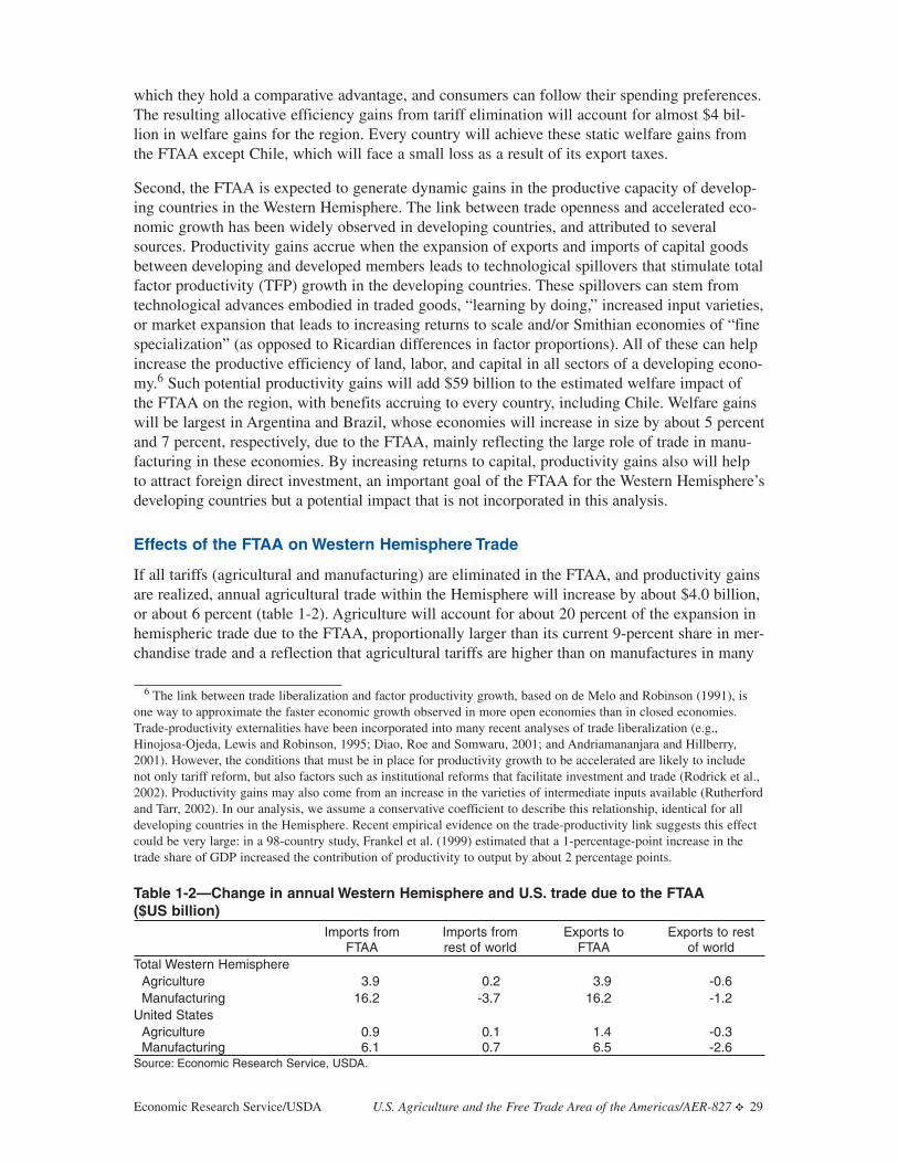
which they hold a comparative advantage, and consumers can follow their spending preferences.The resulting allocative efficiency gains from tariff elimination will account for almost $4 bil-lion in welfare gains for the region. Every country will achieve these static welfare gains fromthe FTAA except Chile, which will face a small loss as a result of its export taxes.

Second, the FTAA is expected to generate dynamic gains in the productive capacity of develop-ing countries in the Western Hemisphere. The link between trade openness and accelerated eco-nomic growth has been widely observed in developing countries, and attributed to severalsources. Productivity gains accrue when the expansion of exports and imports of capital goodsbetween developing and developed members leads to technological spillovers that stimulate totalfactor productivity (TFP) growth in the developing countries. These spillovers can stem fromtechnological advances embodied in traded goods, “learning by doing,” increased input varieties,or market expansion that leads to increasing returns to scale and/or Smithian economies of “finespecialization” (as opposed to Ricardian differences in factor proportions). All of these can helpincrease the productive efficiency of land, labor, and capital in all sectors of a developing econo-my.6 Such potential productivity gains will add $59 billion to the estimated welfare impact ofthe FTAA on the region, with benefits accruing to every country, including Chile. Welfare gainswill be largest in Argentina and Brazil, whose economies will increase in size by about 5 percentand 7 percent, respectively, due to the FTAA, mainly reflecting the large role of trade in manu-facturing in these economies. By increasing returns to capital, productivity gains also will helpto attract foreign direct investment, an important goal of the FTAA for the Western Hemisphere’sdeveloping countries but a potential impact that is not incorporated in this analysis.

Effects of the FTAA on Western Hemisphere Trade

If all tariffs (agricultural and manufacturing) are eliminated in the FTAA, and productivity gainsare realized, annual agricultural trade within the Hemisphere will increase by about $4.0 billion,or about 6 percent (table 1-2). Agriculture will account for about 20 percent of the expansion inhemispheric trade due to the FTAA, proportionally larger than its current 9-percent share in mer-chandise trade and a reflection that agricultural tariffs are higher than on manufactures in many


6 The link between trade liberalization and factor productivity growth, based on de Melo and Robinson (1991), isone way to approximate the faster economic growth observed in more open economies than in closed economies.Trade-productivity externalities have been incorporated into many recent analyses of trade liberalization (e.g.,Hinojosa-Ojeda, Lewis and Robinson, 1995; Diao, Roe and Somwaru, 2001; and Andriamananjara and Hillberry,2001). However, the conditions that must be in place for productivity growth to be accelerated are likely to includenot only tariff reform, but also factors such as institutional reforms that facilitate investment and trade (Rodrick et al.,2002). Productivity gains may also come from an increase in the varieties of intermediate inputs available (Rutherfordand Tarr, 2002). In our analysis, we assume a conservative coefficient to describe this relationship, identical for alldeveloping countries in the Hemisphere. Recent empirical evidence on the trade-productivity link suggests this effectcould be very large: in a 98-country study, Frankel et al. (1999) estimated that a 1-percentage-point increase in thetrade share of GDP increased the contribution of productivity to output by about 2 percentage points.

Table 1-2—Change in annual Western Hemisphere and U.S. trade due to the FTAA ($US billion)

Imports from Imports from Exports to Exports to rest FTAA rest of world FTAA of world

Total Western HemisphereAgriculture 3.9 0.2 3.9 -0.6Manufacturing 16.2 -3.7 16.2 -1.2

United StatesAgriculture 0.9 0.1 1.4 -0.3Manufacturing 6.1 0.7 6.5 -2.6


countries and regions, including the United States.7 Annual U.S. agricultural exports to thehemisphere will increase by $1.4 billion (about 6 percent) and imports by about $900 million(about 3 percent).

The increase in U.S. trade with the Western Hemisphere will lead to small adjustments in U.S.trade with the rest of the world. Annual U.S. agricultural exports to non-FTAA countries willdecline about $300 million, and U.S. imports from these markets will increase slightly, about$100 million. On net, the FTAA will increase annual U.S. global agricultural exports andimports by about $1 billion each.

Figure 1-2 shows changes in FTAA members’ global agricultural exports due to the FTAA. Allcountries will increase their agricultural exports to the region, including Mexico, which will facegreater competition in the United States, its main export market, when the preferences it receivesunder NAFTA are extended to other FTAA members. The Andean region and the CentralAmerican/Caribbean region will have among the highest rates of growth in their annual agricul-tural exports (3 percent and 5 percent, respectively), with most export growth destined for theU.S. market. Despite their nonreciprocal preferences in the U.S. market, these regions face U.S.trade barriers on some agricultural products, particularly processed foods. U.S. tariffs are low orzero on most processed food products, but they remain very high on a small number of products.Comprehensive tariff reform in the FTAA can therefore result in additional agricultural exportgrowth by countries that already benefit from preferences.

The Central American/Caribbean and Andean regions will also have relatively large increases inannual agricultural imports under the FTAA (16 percent and 18 percent, respectively), due to therelatively high tariffs they maintain on imports (fig. 1-3). Whereas most other countries in the


Figure 1-2 FTAA members' global agricultural exports would increase $3.3 billion

Source: ERS, USDA.

-0.5 0 0.5 1.0 1.5

U.S.

Canada

Mexico

Cen.Am.& Carib.

Andean

Argentina

Brazil

Chile

Rest. S. Am.

$U.S. billions

Exports to FTAA Exports to rest of world

7 Tariffs on FTAA members’ imports from the Western Hemisphere, by commodity, are found in appendix table 1-1 C.

hemisphere have already liberalized their agricultural trade with major partners, these tworegions receive nonreciprocal trade preferences from the U.S., their major trade partner in thehemisphere, and from Canada.

The expansion of both agricultural exports and imports in the Central American/Caribbean andAndean regions indicates that their agriculture is likely to undergo significant structural changein response to the FTAA, although on net their aggregate agricultural production will expand.Managing the process of structural change will be important for smaller economies. Their transi-tion to a free trade environment has been a critical issue in the FTAA negotiations. FTAA mem-bers have agreed that the trade pact will take into account differences in the levels of develop-ment and size of the economies in the Western Hemisphere, in order to create opportunities forthe full participation of the smaller economies and to increase their level of development. TheU.S. FTAA proposal on market access is intended to facilitate the adjustment of smalleconomies to free regional trade by offering them deeper and faster access to U.S. markets dur-ing the FTAA’s expected transition period to free trade.

The largest agricultural trade impacts of the FTAA will be in processed foods, for which theWestern Hemisphere’s annual global exports will increase by about $1.5 billion, or 3 percent(table 1-3). This export category is a large, heterogeneous sector that includes fruit and vegetablejuices, syrups and confections, flour, baked goods, roasted coffee and teas, sugar and sugar prod-ucts, and orange juice. The Western Hemisphere’s annual global exports of dairy products alsowill have relatively large growth, at about $330 million, or 33 percent, reflecting the high tariffsthat remain on dairy products in the Western Hemisphere. The FTAA’s global exports of “othercrops”—a category that includes fibers, seeds, flowers, and tropical products such as coffee andbananas—will increase by about $235 million, or 3 percent. Global annual grain exports, includ-ing rice, wheat, and other grains, will increase about $460 million, or 6 percent. The commoditycomposition of the region’s import growth due to the FTAA is similar to that of its exports,reflecting that most of the trade expansion is in intraregional trade.


Figure 1-3 FTAA members' global agricultural imports would increase $4.1 billion

Source: ERS, USDA.

$U.S. billions

Imports from FTAA Imports from non-FTAA

-0.2 0.0 0.2 0.4 0.6 0.8 1.0

U.S.

Canada

Mexico

Cen.Am.& Carib.

Andean

Argentina

Brazil

Chile

Rest S. Amer.

Canada’s largest growth in annual global agricultural exports due to the FTAA will be in wheat($110 million); its largest import growth will occur in dairy products ($210 million). Mexico’slargest increases in annual agricultural exports due to the agreement will occur in processedfoods ($45 million) and horticulture ($16 million); its largest annual import growth will occur inprocessed foods ($21 million) and fats and oils ($30 million). Argentina’s largest increases inannual exports due to the FTAA will occur in processed foods ($90 million) and oilseed and fatproducts ($40 million). Brazil’s annual exports of processed foods, which include sugar andorange juice, will increase by $210 million under the agreement.

Effects of the FTAA on U.S. Agriculture

The growth in annual U.S. agricultural exports will be greatest to Central American andCaribbean countries ($650 million, mostly processed foods) and Andean countries ($360 mil-lion, mostly of grains, and oilseeds and products) (figs. 1-4 and 1-5).8 Annual U.S. agriculturalexports to Canada will increase by about $160 million (mostly dairy) in the FTAA. The FTAAwill liberalize sensitive sectors that had been exempted by NAFTA, including Canadian dairy.Annual U.S. agricultural exports to Argentina ($100 million) and Brazil ($120 million) will bemostly in processed foods.

The Central American and Caribbean region also will account for most of the increase in U.S.agricultural imports due to the FTAA ($310 million), followed by increased imports from theAndean region of $170 million annually. Most of the growth in U.S. imports from these twosupplying regions will be in processed food products. Although most U.S. tariffs on processedagricultural imports from these countries are already zero, U.S. preferences generally maintainvery high tariffs on a small number of commodities related to U.S. farm programs including, forexample, chocolate crumb, sweetened cocoa powders, cake mixes and animal feeds made withmilk derivatives.


Table 1-3—Change in annual, global agricultural imports and exports of FTAA members,by commodity ($US million)

Growth in Growth in FTAA members’ FTAA members’

Commodity global exports global importsRice 179.8 200.7Wheat 130.5 183.1Other grains 146.9 191.9Horticulture 205.0 271.9Oilseeds 126.1 166.7Other crops 234.7 325.7Livestock 45.0 100.9Meats 172.2 265.4Oils and fats 261.0 345.4Dairy products 330.1 350.9Processed foods 1,532.9 1,694.1Total 3,364.1 4,096.6Source: Economic Research Service, USDA.

8 Data on changes in U.S. agricultural trade by country and commodity are reported in appendix tables 1-1A and 1-1 B.

U.S. imports from Brazil will increase by about $130 million annually and from Argentina byabout $60 million annually, with both trade flows composed of a variety of nongrain crops,including sugar and other processed food products. U.S. agricultural imports from Mexico willincrease slightly due to the FTAA, by about $15 million annually.


Figure 1-4 Diverse commodity composition of change in annual U.S. agricultural trade due to FTAA

Source: ERS, USDA.

Rice Wheat Other grains

Horti-culture

Oilseeds Other crops

Livestock Meat Oils and fats

Dairy prods.

Processedfoods

-100

0

100

200

300

400

500

600

700

800$U

.S. m

illio

ns

Imports Exports

Figure 1-5Diverse partners account for change in annual U.S. agricultural trade due to FTAA

Source: ERS, USDA.

Canada Mexico C. Amer. & Carib.

Andean Argentina Brazil Chile

Rest ofworld

Rest S.Amer.

$U.S

. mill

ions

-400

-200

0

200

400

600

800

Imports Exports

Because trade with the Western Hemisphere accounts for a small share of U.S. agricultural pro-duction, trade expansion due to the FTAA will have only a small effect on U.S. output. Exceptfor rice, real output changes by less than 1 percent in the aggregate sectors described in thisanalysis, by sector (table 1-4). Increased U.S. exports will lead to a small expansion of output inoilseeds, oils and fats, milk and dairy products.

Inclusion of U.S., Agriculture Maximize Benefits of the FTAA

The participation of the United States in the FTAA will help the Western Hemisphere attain thefull potential benefits of the agreement. The large size of the U.S. economy makes it the singlemost important regional market for the rest of the hemisphere. In agriculture, U.S. participationwill account for about one-third of the region’s global agricultural export growth due to theFTAA and about one-quarter of the region’s global agricultural import growth (table 1-5). ForU.S. trade partners, the potential trade opportunities with the United States will support boththeir efficiency gains based on increased trade and specialization, as well as potential productivi-ty gains linked to the expansion of trade between developing- and developed-country partners.For the United States, participation in the FTAA ensures expansion of both U.S. agriculturalexports and imports. Without U.S. participation, U.S. global agricultural exports would declinebecause of the preferential treatment that will be extended to competing suppliers within theWestern Hemisphere through the terms of the agreement. Also, U.S. agricultural import growth,which lowers costs and increases variety for consumers, would be diminished.

Agriculture is often a sensitive sector in free trade agreements because most countries providedomestic support or relatively high trade protection to their agricultural producers, and the effec-tiveness of these policies would be compromised by freer trade. Reflecting the diverse levels ofeconomic development of FTAA members, their agricultural policies evidence a range of objec-

tives, including farm income support,reducing price or income variability, pro-viding income and employment in rural orlow-income areas, and stimulating eco-nomic development. While the use of agri-cultural support and protection create chal-lenges for the inclusion of agriculture inthe FTAA, benefits will be greater if agri-culture is included in, rather than excludedfrom, the agreement. Trade liberalizationof manufacturing alone would increaseFTAA members’ demand for manufactur-ing imports, causing some countries toreduce their agricultural production andtrade in order to shift resources into indus-try. This redistribution of agricultural to


Table 1-4—Effects of the FTAA on U.S. agri-cultural production, by sector

Real change Commodity in output (%)Rice 3.2Wheat 0.0Other grains -0.5Horticulture 0.0Oilseeds 0.4Other crops -0.6Livestock -0.4Milk (raw) 0.1Meat -0.3Oils and fats 0.5Dairy products 0.1Processed foods -0.1Source: Economic Research Service, USDA.

Table 1-5—Change in global, annual agricultural trade due to the FTAA, without U.S. par-ticipation and without inclusion of agriculture ($US billion)

U.S. Rest of Western HemisphereExports Imports Exports Imports

FTAA including U.S. and agriculture 1.07 0.97 2.30 3.12FTAA without United States -0.01 0.06 1.47 1.39FTAA without agriculture -0.05 0.12 0.06 0.60


manufacturing production will lead to a small increase in demand for agricultural imports inthese countries. In addition, productivity gains linked to expanded trade in manufacturing sectorswill stimulate consumer demand for all products, including food. The effects of the FTAA onagricultural trade in the Western Hemisphere therefore still will be positive but far smaller ifagriculture is excluded from trade reform. Including agriculture in the FTAA increases thesepositive effects through the potential efficiency and welfare benefits linked directly to agricultur-al trade liberalization.

Doha Development Agenda and the FTAA

FTAA members (except Bermuda) simultaneously are negotiating their regional trade agreementand multilateral policy reforms in the WTO Doha Development Agenda. Globally, the continuedproliferation of regional trade agreements indicates that regionalism and multilateralism havebecome accepted as dual trade strategies for most countries. By May 2003, the WTO had beennotified of 184 regional trade agreements (WTO, 2003). Nearly every country in the world isnow a member of at least one trade agreement (Crawford and Laird, 2001). Nevertheless, thebenefits of a regional versus a multilateral trade strategy is a continuing public policy debate.

Multilateralism will always be a “first best” strategy because it is nondiscriminatory, that is, allcountries participate and offer similar tariff treatment to all WTO members. This principle ofnondiscrimination forms the foundation of today’s global trade rules. Regionalism, on the otherhand, violates this principle by offering preferential tariff treatment to selected trade partners.Opponents of regionalism argue that the creation of trade among a small group of preferredtrade partners is achieved at the expense of trade with and investment in nonmembers.

Advocates of regionalism generally emphasize its incremental and more attainable benefits com-pared with global reform, and its potential role in advancing or strengthening the multilateralprocess. Regional agreements are more likely to achieve deeper and faster reform among like-minded partners than is possible in the more diverse multilateral negotiations. Advocates alsoargue that a region’s successful experience in dealing with nontariff barriers following theremoval or reduction of regional tariffs can provide experience that strengthens the multilateralprocess. The newer regional agreements formed in the past decade, particularly those in theWestern Hemisphere, have also helped to accelerate economic growth in small economies, bylocking in unilateral reforms, stimulating investment and productivity growth, and fostering theirlinks with large and more developed economies (Ethier, 2001). For small, reforming countriesespecially, regionalism can play a role as a first step in engaging in the global trading system,and it helps give such countries a greater stake in a rules-based global trading system. Traderules that ensure predictability and fairness in trade relationships, and that offer a credibleenforcement mechanism, provide conditions that are favorable for the conduct of business,investment, and the expansion of trade.

As the Western Hemisphere pursues a regional agreement, two factors make multilateral agricul-tural reform of continued importance for FTAA members. First, FTAA countries are global agri-cultural traders. They depend on non-FTAA markets, with about 65 percent of their agriculturalexports destined for, and 35 percent of their agricultural imports originating from, outside theWestern Hemisphere. Non-FTAA markets are especially important for the United States andBrazil, for whom they account for 75 percent to 80 percent of their total agricultural exports.The FTAA region is also a major trade bloc in global agricultural markets. Their agriculturalexports outside the Western Hemisphere account for about 45 percent of world agriculturaltrade, and their imports from the rest of the world account for about 9 percent of that trade.


The Western Hemisphere’s position as a large net agricultural exporter gives it a great stake inWTO negotiations that may further liberalize global agricultural markets. Despite the reformsachieved in the Uruguay Round, these markets are still characterized by significant policy distor-tions (USDA, 2001). Further multilateral reform will impose disciplines on FTAA members andthe rest of the world alike. However, in general, the level of distorting policies used by FTAAmembers is lower than in most other countries and regions. The average, post-Uruguay Roundbound agricultural tariff of FTAA countries of about 40 percent is lower than the global averagebound rate of 62 percent (Gibson et al., 2001). The average applied rate of FTAA countries isabout 13 percent. Domestic support in the FTAA is also relatively low. The 2002 producer sup-port estimates for the three FTAA members of the Organization for Economic Cooperation andDevelopment (OECD) are 18 percent (United States), 20 percent (Canada), and 22 percent(Mexico)—below the aggregate OECD rate of 31 percent (OECD, 2003). Finally, export subsi-dies by FTAA members are minimal, with the EU accounting for over 90 percent of globalexpenditure on these subsidies in 1998 (USDA, 2001).

These patterns in agricultural trade flows and agricultural policy distortions suggest that theregion will benefit from additional global trade reforms. Any scenario of globalized reformshows the benefits of a multilateral agreement for the Western Hemisphere. For example, if theDoha Development Agenda replicates the limits set in the Uruguay Round, the region’s annualagricultural exports outside the Western Hemisphere would increase by 10 percent and itsimports by 2 percent. Western Hemisphere agricultural export growth in this scenario for multi-lateral reform is estimated to account for about 40 percent of the resulting expansion of globalagricultural trade.

The multilateral negotiations also have significance for the FTAA because of their more compre-hensive agenda for agricultural reform. The Doha Round is negotiating disciplines on marketaccess, domestic support, and export subsidies. While the mandate for the FTAA includes exportsubsidies in the region and other practices that distort trade in agricultural products, its regionalscope means that it is difficult for the FTAA to limit members’ domestic support for their agri-cultural sectors. In addition, the FTAA cannot address the use of export subsidies by non-FTAAcountries that affect competition within the Western Hemisphere and in third-party markets.

FTAA members recognize the global character of their agricultural markets and the importanceof third-country policies. At the Toronto Trade Ministerial Meeting in 1999, FTAA membersagreed to work in the multilateral negotiations toward the global elimination of export subsidieson agricultural products. FTAA members addressed the problem of domestic support at theQuito Trade Ministerial Meetings in November 2002. There, members agreed on the need forsignificant results in the negotiations on agriculture both in the FTAA and the WTO, and notedthat progress in the FTAA’s market-access negotiations for agriculture will depend on progressbeing made on a broader agriculture agenda. This interdependence of the regional and multilat-eral negotiations increases the Western Hemisphere’s stake in the Doha Development Agenda.

Conclusion

As trade becomes increasingly important for both U.S. agricultural producers and consumers,the potential benefits from the U.S. pursuit of a more open and market-oriented global tradingsystem become greater. U.S. producers will benefit directly from their greater access to worldmarkets and indirectly from the economic growth and increased demand for food that trade lib-eralization can foster. Consumers will benefit because global trade rules help to increase productvariety, lower food costs, and ensure the safety and security of food supplies. The U.S. pursuit ofregionalism complements its pursuit of multilateralism. The dual pursuits reinforce the same



principles of trade liberalization, with regionalism offering an opportunity to achieve deeperreforms on key issues with some partners. Multilateralism provides the venue for more compre-hensive and inclusive, but likely more gradual, trade liberalization, and it can help minimize thepotential negative impacts of regionalism.

This analysis focused on market access reforms in the FTAA. Market access is only one elementof the FTAA negotiations, which also could address other areas that may affect trade in thehemisphere. Furthermore, trade is analyzed in this paper at relatively aggregate levels. For someindividual commodities, complex trade policies and domestic programs will likely influenceboth the liberalization process and the potential trade flows in the FTAA. For these commodi-ties, the results reported here can be only indicative of broad market trends in a free trade area.

References

Andriamananjara, Soamiely and Russell Hillberry. 2001. “Regionalism, Trade and Growth: TheCase of the EU-South Africa Free Trade Arrangement.” U.S. International Trade Commission.Office of Economics working paper No. 01-07-A.

Burfisher, Mary, Sherman Robinson, and Karen Thierfelder. 2002. “The Global Impacts of FarmPolicy Reforms in OECD Countries.” American Journal of Agricultural Economics, Vol. 84, No.3 (August), pp. 234-241.

Crawford, Jo-Anne, and Samuel Laird. 2001. “Regional Trade Agreements and the WTO.” NorthAmerican Journal of Economics and Finance. Vol. 12, No. 2: 193-211.

De Melo, Jaime and Sherman Robinson. 1992. “Productivity and Externalities: Models ofExport-Led Growth.” The Journal of International Trade and Economic Development, Vol. 1,No. 1, pp. 41-68.

Ethier, W.J. 2001. “The New Regionalism in the Americas: A Theoretical Framework,” NorthAmerican Journal of Economics and Finance. No.12, Vol.2, pp: 159-172.

Frankel, Jeffrey A. and David Romer. 1999. “Does Trade Cause Growth?” American EconomicReview, Vol. 89, No. 3, pp. 379-399.

Gibson, Paul, John Wainio, Daniel Whitley and Mary Bohman. 2001. Profiles of Tariffs inAgricultural Markets. U.S. Department of Agriculture, Economic Research Service. AER No.796. Washington, D.C.

Global Trade Analysis Project (GTAP). Base data for 1997, Version 5.1. August, 2002.

Hinojosa-Ojeda, Raul, Jeffrey D. Lewis and Sherman Robinson. 1995. “Regional Integration andOptions for Central America and The Caribbean After NAFTA.” North American Journal ofEconomics and Finance. Vol. 6, No. 2, pp. 121-148.

Lewis, Jeffrey D., Sherman Robinson, and Karen Thierfelder. 2003. “Free Trade Agreementsand the SADC Economies,” Journal of African Economies, Vol. 12, no. 2, pp. 156-206.

Organization for Economic Cooperation and Development (2002). 2001 Producer and ConsumerSubsidy Equivalent electronic database.

Organization for Economic Cooperation and Development (2003). 2002 Producer and ConsumerSubsidy Equivalent electronic database.

Rodrik, Dani, Arvind Subramanian, and Francesco Trebbi. 2002. “Institutions Rule: ThePrimacy of Institutions over Geography and Integration in Economic Development.” NBERWorking Paper No. 9305.

Rutherford, Thomas F. and David G. Tarr. 2002. “Trade Liberalization, Product Variety andGrowth in a Small Open Economy: A Quantitative Assessment,” Journal of InternationalEconomics. Vol. 56, pp. 247-272.

Stout, James V. and Julieta Ugaz-Pereda. 1998. “Western Hemisphere Trading Blocs and TariffBarriers for U.S. Agricultural Exports,” in Regional Trade Agreements and U.S. Agriculture.U.S. Department of Agriculture, Economic Research Service.. AER No. 771. Washington, D.C.

United States Department of Agriculture, Economic Research Service. 2001. Agricultural PolicyReform in the WTO: The Road Ahead. AER No. 802. Washington, D.C.

United States Office of Management and Budget. 2003. Budget of the United States for Fiscal2003. Historical Tables.


Chapter 2

Trade Liberalization in the Western Hemisphere:Impacts on U.S. Agricultural ExportsSteven Zahniser, Daniel Pick, Greg Pompelli, and Mark Gehlhar

Experience with the regional trade agreements already in effect in the Western Hemisphere sug-gests that the trade effects of the FTAA will exceed the impact of its tariff and quota changes.For instance, to the extent that the FTAA requires closer cooperation on sanitary and phytosani-tary issues, as is the case with the North American Free Trade Agreement (NAFTA), membercountries are likely to adjust their import standards so that they do not restrict trade unnecessari-ly. Moreover, the FTAA is likely to have a myriad of indirect effects that ultimately expandtrade, even though these changes may not be spelled out in the agreement. Many developmentsof this sort took place following the implementation of NAFTA and the Common Market of theSouth (MERCOSUR, or Mercado Común del Sur). Examples include increased investor confi-dence within the two regions, the further exploitation of scale economies, and the upgrading oftransportation linkages along new and existing routes of trade.

To better understand the potential breadth of the FTAA’s influence, this chapter assesses theimpact that NAFTA, MERCOSUR, and related agreements have had on agricultural trade withinthe Western Hemisphere. Focusing on U.S. agricultural exports from 1980 through 1999, thechapter employs a series of modified gravity models, as suggested by Cheng and Wall (1999), toidentify noteworthy changes in trade coinciding with these agreements. A main strength of thisapproach is that it distinguishes the impact of a trade agreement on U.S. exports to a specificcountry from the relative closeness of that country’s bilateral trade relationship with the UnitedStates. However, the variables used to identify trade agreements may also capture the influenceof other factors that were contemporaneous to these reforms.

To develop a complete picture of regionalism’s impact on U.S. agricultural exports, separatemodels are estimated at the aggregate level and for 32 individual commodities. This analysisgenerates several important findings:

(1) Unilateral trade reforms undertaken by Mexico during the late 1980s and early 1990shave provided a sizable boost to U.S. agricultural exports to Mexico. According to grav-ity-model estimates, these unilateral reforms accounted for 39 percent of U.S. agricul-tural exports to Mexico from 1989 through 1999, or an average of roughly $1.7 billionper year. Thus, one of NAFTA’s main benefits to U.S. agriculture has been to “lock in”reforms that Mexico had made prior to NAFTA.

(2) NAFTA’s estimated influence on U.S. agricultural exports to Mexico is positive and sta-tistically significant for four of the commodities studied (grapes, tobacco products, yarnand thread, and leather), and it is positive but statistically insignificant for 18 other com-modities. Although the model differentiates NAFTA and Mexico’s unilateral reforms,both were components of an integrated strategy for market reform that Mexico has pur-sued since the mid-1980s. Mexican trade liberalization, both unilateral and throughNAFTA, accounted for an average annual increase in U.S. agricultural exports toMexico of $3.1 billion during 1994-99.

(3) The estimated impact of the Canada-U.S. Free Trade Agreement (CFTA) and NAFTAon U.S. agricultural exports to Canada is not statistically significant. This finding,


which is observed both at the aggregate level and for all the individual commoditiesstudied, may reflect the fact that most barriers to U.S.-Canada agricultural trade wererelatively low prior to CFTA, while several important sectors—dairy, poultry, andeggs—were exempted from trade liberalization.

(4) MERCOSUR’s application of a common external tariff has lowered some barriers toU.S. agricultural exports, creating new opportunities for trade. Relatively high levels ofU.S. agricultural exports during the MERCOSUR period are observed at the commoditylevel for all four MERCOSUR countries and at the aggregate level for Argentina,Paraguay, and Uruguay. In the cases of Argentina and Brazil, several consumer-orientedfood products from the United States appear to have benefited from tariff reductionslinked to MERCOSUR’s common external tariff, although the value of this trade is stillsmall compared with exports to Canada and Mexico.

(5) MERCOSUR appears to have had a trade-diverting effect on U.S. wheat exports toBrazil. With the creation of MERCOSUR, Argentina has dramatically increased itsshare of the Brazilian wheat market, while U.S. wheat exports to Brazil have declined.Argentine wheat enters Brazil duty free, while U.S. wheat faces MERCOSUR’s com-mon external tariff for the product.

The rest of the chapter contains a methodological overview of the modified gravity models andan extensive discussion of their findings. Technical aspects of the models are discussed in appen-dix 2-1, while the International Bilateral Agricultural Trade (IBAT) database, the source of theexport data used in the chapter, is profiled in appendix 2-2.

Gravity Model Methodology

In its most basic application, the gravity model of international trade posits that the level ofexports from one country to another is a function of each country’s gross domestic product(GDP) and its population, as well as the distance between the two countries. To estimate thetrade effects of regional trade agreements, a number of “gravity modelers” (such as Frankel,1997; Endoh, 1999; and Soloaga and Winters, 2001) have included additional explanatory vari-ables that indicate a country’s membership in a specific trade agreement or trade bloc. Thesevariables, however, do not distinguish the influence of a trade agreement from the long-term, rel-ative closeness of a specific bilateral trading relationship. Nor do they account for the stronglikelihood that the impact of a trade agreement varies from one participant to another.

To overcome these shortcomings, this chapter features a different specification of the gravitymodel (table 2-1). Following Cheng and Wall, the modified models include two sets of fixedeffects (variables with the value of one or zero) that respectively identify specific importingcountries and specific years. The fixed effects for importing country play a crucial role in theanalysis, as they control for the importing country’s long-term bilateral trading relationship withthe United States. This increases the likelihood that the trade-agreement variables capture theeffects of those agreements, rather than the general closeness of a particular bilateral relation-ship. Moreover, the trade-agreement variables are country-specific in order to address the possi-bility that the impact of an agreement varies among its participants. Table 2-2 provides a defini-tion of each trade-agreement variable.

While the modified gravity models provide an improved framework for assessing regional tradeagreements, the trade-agreement variables may still capture the influence of unrelated develop-ments that are contemporaneous to these accords. Unusual weather patterns are an obvious



Table 2-1—Comparison of basic and modified gravity models

Basic gravity model

Dependent variable: Log of exports from country i to country j

Explanatory variables: InterceptLog of GDP of country iLog of GDP of country jLog of population of country iLog of population of country jLog of distance between country i and country jOther variables selected by researcher, such as dummy variables to denote trade flows corresponding to particular trade agreements

Econometric Approach: Ordinary least squares (usually)

Modified gravity model, as used in this chapter

Dependent variable: Log of U.S. agricultural exports to country i in year t(in U.S. dollars)

Explanatory variables: InterceptLog of GDP of country i in year t (in U.S. dollars)Fixed effects denoting importing country

For example, the fixed effect for Mexico equals one if Mexico is the importing country and zero otherwise. For purposes of comparison, no fixed effect is included for Canada.

Fixed effects denoting yearFor example, the fixed effect for 1998 equals one if the year is 1998 and zero otherwise. For purposes of comparison, no fixed effect is included for 1999.

Trade-agreement variables – dummy variables that identify country i’s participation in a particular trade agreement in year t

Econometric approach: TobitSource: Economic Research Service.

Table 2-2—Trade-agreement variables in the modified gravity models

NAFTA countriesUnilateral-Mexico Equals one for exports to Mexico during 1989-99 and zero otherwiseNAFTA-Mexico Equals one for exports to Mexico during 1994-99 and zero otherwiseCFTA-Canada Equals one for exports to Canada during 1989-99 and zero otherwiseNAFTA-Canada Equals one for exports to Canada during 1994-99 and zero otherwise

MERCOSUR countriesFull members:

Argentina/1991-99 Equals one for exports to Argentina during 1991-99 and zero otherwiseArgentina/1994-99 Equals one for exports to Argentina during 1994-99 and zero otherwiseBrazil/1991-99 Equals one for exports to Brazil during 1991-99 and zero otherwiseBrazil/1994-99 Equals one for exports to Brazil during 1994-99 and zero otherwiseParaguay/1991-99 Equals one for exports to Paraguay during 1991-99 and zero otherwiseParaguay/1994-99 Equals one for exports to Paraguay during 1994-99 and zero otherwiseUruguay/1991-99 Equals one for exports to Uruguay during 1991-99 and zero otherwiseUruguay/1994-99 Equals one for exports to Uruguay during 1994-99 and zero otherwise

Associate members:Bolivia/1997-99 Equals one for exports to Bolivia during 1997-99 and zero otherwiseChile/1996-99 Equals one for exports to Chile during 1996-99 and zero otherwise

Source: Economic Research Service.

example of an unrelated phenomenon that causes short-term changes in agricultural productionand trade, and less experienced observers might incorrectly attribute these changes to one ormore trade agreements. By having encompassing measures of the effects of trade-policyreforms, the modified gravity models may offer better estimates of their impact than models thatfocus narrowly on tariff reductions. However, these measures may be so broad that they capturethe influence of factors that have little to do with trade agreements.

Empirical Findings

Total Agricultural Exports. Table 2-3 summarizes the results from the model of total U.S. agri-cultural exports. Although each variable denoting exports to Canada or Mexico during theCFTA/NAFTA period obtains a positive coefficient, only the coefficient for Unilateral-Mexico isstatistically significant. Thus, the model supports the theory that Mexico’s unilateral reformshave boosted U.S. agricultural exports to Mexico since 1989. It also suggests that the role ofNAFTA in “locking-in” Mexico’s earlier reforms was an important one.1

Figure 2-1 contrasts the actual and expected values of U.S. agricultural exports to Mexico from1980 through 1999, based on the coefficients from the model. The figure illustrates that themodified gravity model does a reasonably good job of capturing the broad features of this trade,given the relative simplicity of the model and the coarseness of the trade-agreement variables.The largest difference between the actual and predicted values occurs in 1995, right after thesudden devaluation of the Mexican peso in December 1994. This suggests that the inclusion ofan exchange-rate variable might improve the performance of the modified gravity model.

Using the coefficients for Unilateral-Mexico and NAFTA-Mexico, one may calculate the expect-ed value of U.S. agricultural exports to Mexico when these variables are held to zero.2 This sim-ulation reveals that the model attributes a great deal of influence to Unilateral-Mexico andNAFTA-Mexico. Mexico’s unilateral reforms account for 39 percent of U.S. agricultural exportsto Mexico during 1989-1993, while the reforms and NAFTA together account for 59 percent ofthis trade during 1994-99.3 These percentages correspond to additional trade flows worth anaverage of $1.3 billion per year during 1989-93 and $3.1 billion per year during 1994-99. Theimpact of the unilateral reforms alone averages $1.7 billion per year during 1989-1999.

The simulation also provides an estimate (albeit insignificant) of NAFTA’s impact on U.S. agri-cultural exports to Mexico. According to the model, NAFTA accounts for 20 percent of thistrade during 1994-99. This estimate is substantially larger than the assessment of ERS’s 1997NAFTA Report (Crawford and Link, 1997), which concludes that U.S. agricultural exports toMexico in 1996 were about 3 percent higher than they would have been in NAFTA’s absence.This analysis relied upon a computable general equilibrium model and only examined the first 3years of NAFTA’s 14-year transition to trade liberalization. Based on careful consideration of


1 A sample with more observations of U.S. agricultural exports to Canada and Mexico during the CFTA-NAFTAperiod might afford more precise estimates of these coefficients. To explore this possibility, an alternative model wasestimated using the data for all 32 commodity groupings, but this model also yielded insignificant coefficients forCFTA-Canada, NAFTA-Canada, and NAFTA-Mexico. However, these coefficients were significant in another alterna-tive model, estimated using ordinary least squares, in which the original sample was limited to countries with agricul-tural imports from the United States of at least $500 million. The results from both models are available from theauthors.

2 Appendix 2-1 describes this calculation in greater detail.3 A one-tailed t-test supports the joint hypothesis that the coefficients of Unilateral-Mexico and NAFTA-Mexico in

Model 1 are greater than zero at the 90-percent confidence level, even though NAFTA-Mexico’s coefficient by itselfdoes not pass such a test.

NAFTA’s commodity-specific provisions, ERS’s 2002 NAFTA Report (Zahniser and Link, 2002)identifies several U.S. agricultural exports to Mexico whose trade volume during 1994-2000increased by more than 15 percent as a direct result of NAFTA: rice, dairy products, cotton,processed potatoes, apples, and pears.

Figure 2-2 presents a similar simulation of U.S. agricultural exports to Canada in the absence ofCFTA and NAFTA. Although the coefficients for CFTA-Canada and NAFTA-Canada are notstatistically significant, the trade effects associated with these coefficients are large in value.Specifically, the model attributes an annual average of $2.3 billion of U.S. agricultural exports toCanada during 1989-1999 to the two agreements. Since 1985, U.S. agricultural exports toCanada have increased steadily and without interruption, a pattern that may correspond to theinsignificance of CFTA-Canada and NAFTA-Canada.


Table 2-3—Parameter estimates for gravity models of total U.S. agricultural exports

Variable Parameter Estimate Standard Error Interpretation

Number of observations 2,540Number of left-censored observations 5Intercept 12.7975 0.3690 ***Log of importing country’s GDP 0.3183 0.0438 *** U.S. agricultural exports increase

with the importing country’s GDP

Participation in NAFTA or MERCOSUR Impact on U.S. agricultural exports:

CFTA-Canada (1989-99) 0.3758 0.3758 InsignificantNAFTA-Canada (1994-99) 0.3028 0.4081 InsignificantUnilateral-Mexico (1989-99) 0.4987 0.3759 * PositiveNAFTA-Mexico (1994-99) 0.3892 0.4080 InsignificantArgentina, 1991-99 1.0117 0.4390 *** PositiveArgentina, 1994-99 0.7019 0.4764 * PositiveBrazil, 1991-99 -0.9025 0.4397 ** NegativeBrazil, 1994-99 0.8627 0.4764 ** PositiveParaguay, 1991-99 1.5880 0.4389 *** PositiveParaguay, 1994-99 0.2927 0.4765 InsignificantUruguay, 1991-99 0.0012 0.4390 InsignificantUruguay, 1994-99 0.6360 0.4765 * PositiveBolivia, 1997-99 -0.3799 0.4219 InsignificantChile, 1996-99 0.1391 0.3770 Insignificant

Fixed effects for importing country Compared with exports to Canada, U.S. agriculture is:

Argentina -4.2950 0.3059 *** Less likely to export to ArgentinaBolivia -3.0016 0.3403 *** Less likely to export to BoliviaBrazil -1.8809 0.3021 *** Less likely to export to BrazilChile -2.4824 0.3032 *** Less likely to export to ChileMexico -0.2212 0.3178 Just as likely to export to MexicoParaguay -5.5870 0.3617 *** Less likely to export to ParaguayUruguay -4.9627 0.3477 *** Less likely to export to UruguayScale 0.6710Log-likelihood -2,595.8n.a. = not applicableCoefficients for fixed effects for year and some fixed effects for importing country are not reported.Results of one-tailed t-test of parameter estimate’s significance:***Passes at 99-percent confidence level; **passes at 95-percent level; and *passes at 90-percent level.Source: Economic Research Service.

MERCOSUR appears to have had a trade-creating effect on U.S. agricultural exports toArgentina, Uruguay, and Paraguay. This trade has grown dramatically since MERCOSUR’simplementation, but each of these countries is still a relatively minor market for U.S. agriculturalproducts, especially when compared with Canada or Mexico. According to the IBAT database,U.S. agricultural exports to these three countries totaled $176 million in 1999, compared with$13.2 billion for Canada and Mexico combined. Argentina is the largest customer of U.S. agri-cultural products in MERCOSUR, with agricultural imports from the United States totaling$154 million in 1999. A simulation of this trade in MERCOSUR’s absence suggests that thecommon market increased U.S. agricultural exports to Argentina by an average of $117 millionper year during 1991-99 (fig. 2-3).

MERCOSUR’s positive influence on U.S. exports probably stems from the common market’s exter-nal tariff. In many instances, this external tariff is substantially lower than the tariffs previouslyapplied individually by MERCOSUR’s member countries. For example, Argentina’s average appliedtariff rate dropped from 20 percent to 10 percent between 1987 and 1995, while Brazil lowered itsaverage from 58 percent in 1986 to 10 percent in 1995 (Stout and Ugaz-Pereda, 1998: p. 134).However, the model suggests that MERCOSUR has diverted U.S. agricultural exports away fromBrazil, especially during 1991-93 (fig. 2-4). The initial decline in this trade corresponds not with thestart of the common market in 1991 but instead with the year 1987. Thus, factors other than MER-COSUR may be partially responsible for the reduced level of exports. In addition, the commoditymodels analyzed below indicate that developments in wheat trade account for a substantial portionof the negative effect associated with MERCOSUR.


Figure 2-1 Actual and expected values of U.S. agricultural exports to Mexico, 1980-1999

0

1

2

3

4

5

6

7

1980 1982 1984 1986 1988 1990 1992 1994 1996 1998

$U.S

. bill

ions

Actual exports As predicted by model Simulation, No Unilateral Reforms, No NAFTA


One additional result of interest lies among the fixed effects for importing country. Each fixedeffect for the MERCOSUR countries is negative and strongly significant, a result that should notbe surprising given that the excluded country for purposes of comparison is Canada. But thecoefficient for exports to Mexico is statistically indistinguishable from zero. This suggests thatthe long-term U.S. trading relationship with Mexico is about as close as the long-term relation-ship with Canada, once the size of the two economies and the differing impacts of CFTA,NAFTA, and Mexico’s unilateral reforms are taken into account.

Commodity Models. To explore the impact of regional trade agreements at the commoditylevel, we estimate 32 additional models, each for a specific commodity or group of commodi-ties. Table 2-4 summarizes the results of these models with respect to the trade-agreement vari-ables. As a group, these models provide additional support for the hypothesis that Mexico’s uni-lateral trade reforms have strengthened U.S. agricultural exports to that country. Unilateral-Mexico obtains a positive and significant coefficient in 14 commodity models: beer, cotton,flowers and foliage, apples, rice, wheat, peanuts, macaroni, beef, pork, prepared breakfast food,soda and bottled water, tobacco, tobacco products, and tomatoes. In contrast, NAFTA-Mexico ispositive and significant in only four commodity models (grapes, yarn and thread, leather, andtobacco products), but it is positive and insignificant for 18 other commodities.4


Figure 2-2 Actual and expected values of U.S. agricultural exports to Canada, 1980-1999

$U.S

. bill

ions

Actual exports As predicted by model Simulation, No CFTA or NAFTA

0

1

2

3

4

5

6

7

8

1980 1982 1984 1986 1988 1990 1992 1994 1996 1998


4 The 18 commodities include cotton, cut flowers, fruit or vegetable juice, apples, corn, rice, wheat, peanuts, beef,poultry meat, plants and bulbs, prepared breakfast food, soybean oil, soybeans, sunflower seed oil, raw tobacco, toma-toes, and legumes.

Given ERS’s previous research about NAFTA, it is not surprising that grapes and yarn and threadare among the commodities where NAFTA-Mexico is significant. The 2002 NAFTA reportdescribes Mexico’s elimination of its import-licensing requirement for U.S. grapes as an impor-tant element of NAFTA. It also emphasizes the importance of NAFTA’s rules of origin for textilesand apparel, which restrict NAFTA trade benefits to articles produced from fabric, yarn, thread,and fiber manufactured in the NAFTA countries. These rules are likely to have boosted demandof Mexican textile and apparel producers for U.S. yarn and thread.

But there are also many noteworthy absences from the list of commodities where NAFTA-Mexico is significant. The 2002 NAFTA report concludes that NAFTA provided a moderateboost (a 6-percent to 15-percent increase in trade volume during 1994-2000) to U.S. exports toMexico of corn, oilseeds, beef, and sorghum. They also indicate that NAFTA provided a strongboost (more than 15 percent) to U.S. exports to Mexico of rice, dairy products, cotton, processedpotatoes, apples, and pears. These findings suggest that the commodity models in this chapterwould benefit from a NAFTA variable that more precisely measures the agreement’s commodi-ty-specific provisions.

Similar to the model of total agricultural exports, the commodity models provide no evidencethat CFTA and NAFTA have had a significant impact on U.S. agricultural exports to Canada.The coefficient for CFTA-Canada is positive in 8 commodity models, while the coefficient forNAFTA-Canada is positive in 20 commodity models. However, none of these coefficients arestatistically significant. Again, these results differ from ERS’s commodity-level assessments of


Figure 2-3 Actual and expected values of U.S. agricultural exports to Argentina, 1980-1999

Actual exports As predicted by model Simulation, No MERCOSUR

0

50

100

150

200

250

300

350

1980 1982 1984 1986 1988 1990 1992 1994 1996 1998

$U.S

. mill

ions


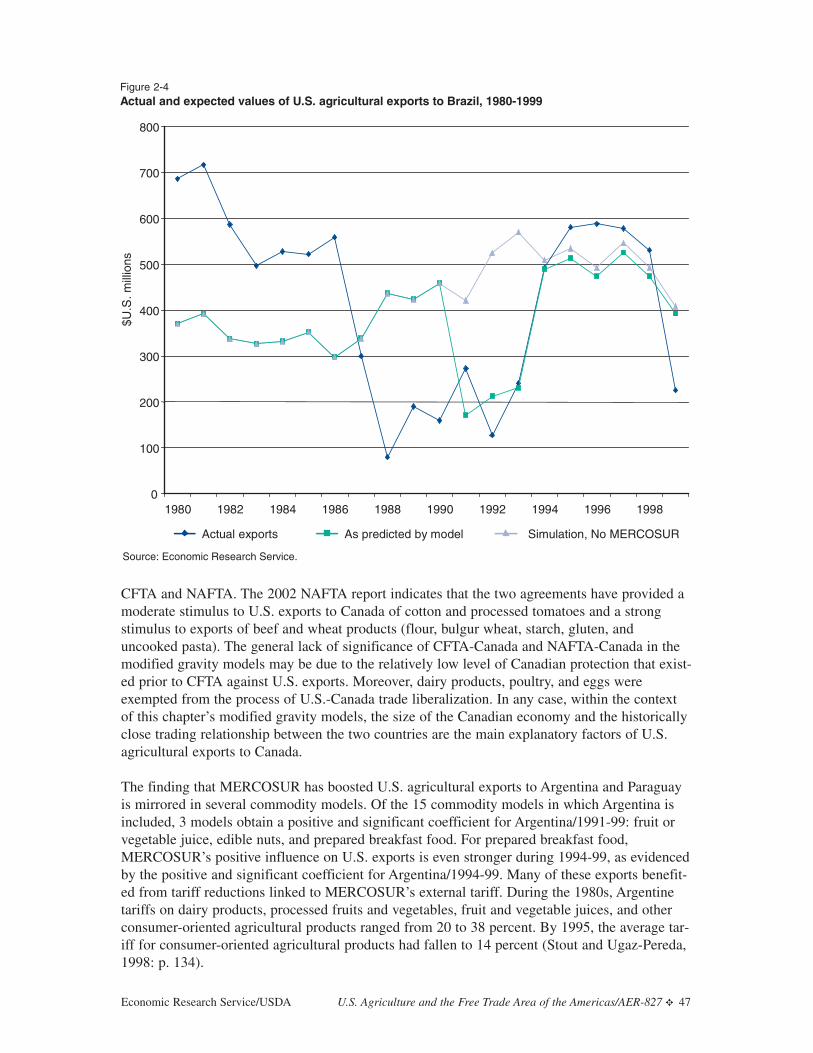
CFTA and NAFTA. The 2002 NAFTA report indicates that the two agreements have provided amoderate stimulus to U.S. exports to Canada of cotton and processed tomatoes and a strongstimulus to exports of beef and wheat products (flour, bulgur wheat, starch, gluten, anduncooked pasta). The general lack of significance of CFTA-Canada and NAFTA-Canada in themodified gravity models may be due to the relatively low level of Canadian protection that exist-ed prior to CFTA against U.S. exports. Moreover, dairy products, poultry, and eggs wereexempted from the process of U.S.-Canada trade liberalization. In any case, within the contextof this chapter’s modified gravity models, the size of the Canadian economy and the historicallyclose trading relationship between the two countries are the main explanatory factors of U.S.agricultural exports to Canada.

The finding that MERCOSUR has boosted U.S. agricultural exports to Argentina and Paraguayis mirrored in several commodity models. Of the 15 commodity models in which Argentina isincluded, 3 models obtain a positive and significant coefficient for Argentina/1991-99: fruit orvegetable juice, edible nuts, and prepared breakfast food. For prepared breakfast food,MERCOSUR’s positive influence on U.S. exports is even stronger during 1994-99, as evidencedby the positive and significant coefficient for Argentina/1994-99. Many of these exports benefit-ed from tariff reductions linked to MERCOSUR’s external tariff. During the 1980s, Argentinetariffs on dairy products, processed fruits and vegetables, fruit and vegetable juices, and otherconsumer-oriented agricultural products ranged from 20 to 38 percent. By 1995, the average tar-iff for consumer-oriented agricultural products had fallen to 14 percent (Stout and Ugaz-Pereda,1998: p. 134).


Figure 2-4 Actual and expected values of U.S. agricultural exports to Brazil, 1980-1999

Actual exports As predicted by model Simulation, No MERCOSUR

0

100

200

300

400

500

600

700

800

1980 1982 1984 1986 1988 1990 1992 1994 1996 1998

$U.S

. mill

ions


In the model of U.S. soybean exports, the coefficient for Argentina/1994-99 is positive andstrongly significant, which at first glance suggests that MERCOSUR has had a positive impacton this trade. However, the significance of this coefficient is more likely due to a severe droughtthat sharply reduced the size of Argentina’s 1996/97 soybean crop (U.S. Department ofAgriculture, Foreign Agricultural Service, 1997). As a result, U.S. soybean exports to Argentina,usually less than $200,000 per year, climbed to $124 million in 1997 and $10 million in 1998.Only the commodity model for raw tobacco shows that MERCOSUR has depressed U.S. exportsto Argentina. U.S.-Argentina trade in this commodity was customarily small during 1980-1999,with exports to Argentina never exceeding $500,000 per year.


Table 2-4—Overview of commodity-specific gravity models of U.S. agricultural exports

ParameterUnilateral- NAFTA- Argentina, Argentina, Brazil, Brazil,

Model Mexico Mexico 1991-99 1994-99 1991-99 1994-99Total agricultural exports Positive Insig. Positive Insig. Negative PositiveBeer Positive Insig. n.a. n.a. n.a. n.a.Cheese Insig. Insig. n.a. n.a. Positive PositiveDistilled alcoholic beverages Insig. Insig. Insig. Insig. Positive PositiveCotton Positive Insig. Insig. Insig. Insig. Insig.Flowers and foilage (cut) Positive Insig. n.a. n.a. n.a. n.a.Fruit or vegetable juice Insig. Insig. Positive Insig. Positive PositiveApples (fresh) Positive Insig. n.a. n.a. Insig. PositiveGrapes (fresh) Insig. Positive n.a. n.a. Insig. PositiveCorn Insig. Insig. Insig. Insig. Insig. Insig.Rice Positive Insig. n.a. n.a. Positive Insig.Wheat Positive Insig. n.a. n.a. Negative Insig.Peanuts Positive Insig. n.a. n.a. Positive Insig.Leather Insig. Positive Insig. Insig. Insig. Insig.Live poultry Insig. Insig. n.a. n.a. Insig. Insig.Macaroni Positive Insig. Insig. Insig. n.a. n.a.Beef (fresh or frozen) Positive Insig. n.a. n.a. Insig. PositivePork (fresh or frozen) Positive Insig. n.a. n.a. n.a. n.a.Poultry (fresh or frozen) Insig. Insig. n.a. n.a. n.a. n.a.Milk and cream Insig. Insig. Insig. Insig. Negative Insig.Edible nuts Insig. Insig. Positive Insig. Insig. Insig.Plants and bulbs (live) Insig. Insig. Insig. Insig. Insig. PositivePrepared breakfast food Positive Insig. Positive Positive Positive PositiveSoda and bottled water Positive Insig. n.a. n.a. Positive PositiveSoybean oil Insig. Insig. n.a. n.a. n.a. n.a.Soybeans Insig. Insig. Insig. Positive Insig. Insig.Sunflower seed oil Insig. Insig. n.a. n.a. n.a. n.a.Tobacco (unmanufactured) Positive Insig. Negative Positive Insig. Insig.Tobacco products Insig. Positive Insig. Insig. Insig. Insig.Tomatoes Positive Insig. n.a. n.a. n.a. n.a.Legumes Insig. Insig. Insig. Insig. Negative PositiveWine Insig. Insig. n.a. n.a. Insig. PositiveYarn and thread Insig. Positive Insig. Insig. Insig. Insig.n.a. = not applicableSign of parameter estimate and estimate’s significance according to a one-tailed t-test:Insig. = Insignificant at 90-percent levelPositive = Positive coefficient, significant at 90-percent levelNegative = Negative coefficient, significant at 90-percent levelNone of the parameter estimates for CFTA-Canada or NAFTA-Canada are significant.Source: Economic Research Service.

Paraguay appears in just seven commodity models, two of which indicate that MERCOSUR is asignificant factor influencing U.S. exports to that country. First, the common market is found tohave increased U.S. beer exports to Paraguay during 1991-99. This trade averaged $12 millionper year during 1997-99, compared with just $204,000 per year during 1988-1990. Second,MERCOSUR is associated with lower U.S. exports of milk and cream to Paraguay. Like U.S.tobacco exports to Argentina, this trade was extremely small throughout the sample period, lastexceeding $100,000 in 1983.

Although the model for total agricultural exports indicates that MERCOSUR has reduced U.S.exports to Brazil, the commodity models suggest that the common market has stimulated manyaspects of this trade. The coefficient for Brazil/1991-99 is positive and significant for sevencommodities: cheese, distilled alcoholic beverages, fruit or vegetable juice, rice, leather, pre-pared breakfast food, and soda and bottled water. In addition, the coefficient for Brazil/1994-99is positive and significant for 11 commodities: cheese, distilled alcoholic beverages, fruit or veg-etable juice, apples, grapes, beef, plants and bulbs, prepared breakfast food, soda and bottledwater, legumes, and wine. In many instances, U.S. exports of these products are likely to havebenefited from Brazilian tariff reductions associated with MERCOSUR’s common external tar-iff. Stout and Ugaz-Pereda emphasize that Brazil’s applied tariffs on agricultural products priorto MERCOSUR were much higher than Argentina’s, with most tariff rates exceeding 40 percent.

The commodity models also provide evidence that MERCOSUR has limited some U.S. exportsto Brazil, as the coefficient for Brazil/1991-99 is negative and significant in the models forwheat, milk and cream, and legumes. (The coefficient for Brazil/1994-99 is not negative and sig-nificant in any of the commodity models.) Among these products, milk and cream and legumesare not prominent candidates for trade diversion. Milk and cream exports to Brazil averaged lessthan $1 million per year during 1988-90 and only $3 million per year during 1997-99. Legumeexports to Brazil actually have grown under MERCOSUR, from an average of $2 million peryear during 1988-90 to $6 million per year during 1997-99.

Wheat, in contrast, is a completely different case. U.S. wheat exports to Brazil dropped from anannual average of $23 million during 1988-90 to just $4 million during 1997-99. Across thesame two periods, Argentine wheat exports to Brazil surged from $183 million to $801 millionper year. MERCOSUR’s tariff preference partially explains this shift, as the common market’sexternal tariff for wheat equaled 11.5 percent in 2002 (Svec, 2002: p. 12). But improved wheatyields in Argentina also help to explain the changing fortunes of U.S. wheat exports to Brazil. Infact, Argentine wheat producers have nearly closed the yield gap that separates them from theirU.S. counterparts (Schnepf, Dohlman, and Bolling, 2001: pp. 30-31).

Conclusion

The modified gravity models in this chapter highlight a number of important recent developmentsin the pattern of U.S. agricultural exports. First and foremost, exports to Mexico during 1989-1999 are significantly higher than previous exports to Mexico, once the changing size of theMexican economy and the historic closeness of the U.S.-Mexico trading relationship are takeninto account. This result is obtained both at the aggregate level and for 14 different commodities.Unilateral reforms by Mexico to open its market in the late 1980s and early 1990s are responsiblefor most of the heightened level of this trade. The additional trade benefits secured by NAFTAappear to be less important to U.S. agricultural exports to Mexico, providing a significant stimu-lus only to grapes, yarn and thread, leather, and tobacco products. As a practical matter, the uni-lateral and regional trade reforms are both parts of the profound economic reorientation thatMexico has undergone since the late 1980s, and the two types of reform together are found to


have a significant impact on U.S. agricultural exports to Mexico. With the exception of one alter-native model, none of the models associate the CFTA/NAFTA period with a significant change inU.S. agricultural exports to Canada. Previous ERS assessments of NAFTA’s commodity-specificprovisions (included those originally negotiated in CFTA) suggest that CFTA and NAFTA havehad a much broader impact on U.S. agricultural exports to both Canada and Mexico.

The models suggest that MERCOSUR has had a mixed effect on U.S. agricultural exports. Forall four countries, there are commodities where MERCOSUR is linked to increased U.S.exports, and at the aggregate level, MERCOSUR is found to have created trade in the cases ofArgentina, Paraguay, and Uruguay. With respect to Brazil, however, a finding of trade diversionis obtained at the aggregate level and for milk and cream, legumes, and wheat. Among thesecommodities, wheat is the most likely case of trade diversion, as Argentina has dramaticallyincreased its share of the Brazilian wheat market.

Care must be taken in the evaluation of these findings, as the variables that denote the participa-tion of a country in a particular trade agreement also capture the influence of other contempora-neous factors. Incorporating additional variables that more fully describe international marketsfor specific commodities should improve the performance of the models in this chapter.Examples include volume measures of trade, actual transportation costs, levels of production bycountry, changes in yields, the amount of consumption, and quantitative measures of tradeimpediments. Of course, additional data collection usually comes at a cost, and one of the mainattractions of gravity models as they stand is that their data requirements are relatively small.The next generation of gravity models is likely to depart from this tradition.

References

Cheng, I.H., and Howard J. Wall. “Controlling for Heterogeneity in Gravity Models of Trade.”Working Paper 99-010A, Federal Reserve Bank of Saint Louis, February 1999. Accessible at:http://www.stls.frb.org/research/wp/99-010.html.

Crawford, Terry, and John E. Link (coordinators). NAFTA. U.S. Department of Agriculture,Economic Research Service, International Agriculture and Trade Report, Situation and OutlookSeries, WRS-97-2, September 1997. Accessible at: http://www.ers.usda.gov/briefing/nafta/man-dated.htm.

Endoh, Masahiro. “Trade creation and trade diversion in the EEC, the LAFTA and the CMEA:1960-1994.” Applied Economics, Vol. 31 (1999), pp. 207-216.

Frankel, Jeffrey A. Regional Trade Blocs in the World Economic System. Washington: Institutefor International Economics, 1997.

Green, William H. Econometric Analysis. New York: MacMillan Publishing Company, 1990.

International Monetary Fund. “World Economic Outlook Database.” September 2000.Accessible at: http://www.imf.org/external/pubs/ft/weo/2000/02/data/index.htm.

Rosenzweig Pichardo, Andrés. “La Política de Comercio Exterior del Sector Agropecuario deMéxico Durante La Década de los Noventas.” In Andrés Casco and Andrés Rosenzweig (eds.),La Política Sectorial Agropecuaria en México: Balance de una Década, Mexico City: InstitutoInteramericano de Cooperación para la Agricultura, December 2000.


Schnepf, Randall D., Erik N. Dohlman, and Christine Bolling. Agriculture in Brazil andArgentina: Developments and Prospects for Major Field Crops. U.S. Department of Agriculture,Economic Research Service, Market and Trade Economics Divison, Agriculture and TradeReport, WRS-01-3, November 2001.

Soloaga, Isidro, and L. Alan Winters. “Regionalism in the Nineties: What Effect on Trade?”North American Journal of Economics and Finance, Vol. 12, No. 1 (March 2001), pp. 1-29.

Stout, James H., and Julieta Ugaz-Pereda. “Western Hemisphere Trading Blocs and TariffBarriers for U.S. Agricultural Exports.” In Mary E. Burfisher and Elizabeth E. Jones (eds.),Regional Trade Agreements and U.S. Agriculture, U.S. Department of Agriculture, EconomicResearch Service, Market and Trade Economics Division, Agricultural Economic Report No.771 (Washington, DC: November 1998), pp. 131-139.

Svec, Kimberly L. “Brazil: Grain and Feed Annual 2002.” U.S. Department of Agriculture,Foreign Agricultural Service, Global Agriculture Information Network (GAIN) Report No.BR2605, March 25, 2002.

U.S. Department of Agriculture, Foreign Agricultural Service. “Oilseeds: World Markets andTrade,” December 1997. Accessible at http://www.fas.usda.gov/oilseeds/circular/1997/97-12/dec97opd2.htm.

United Nations. Demographic Yearbook. New York: various issues.

United Nations. Statistical Yearbook of the United Nations. New York: various issues.

Zahniser, Steven, and John Link (eds.). Effects of North American Free Trade Agreement onAgriculture and the Rural Economy. U.S. Department of Agriculture, Economic ResearchService, Agriculture and Trade Report, WRS-0201, July 2002. Accessible at:http://www.ers.usda.gov/publications/wrs0201/.


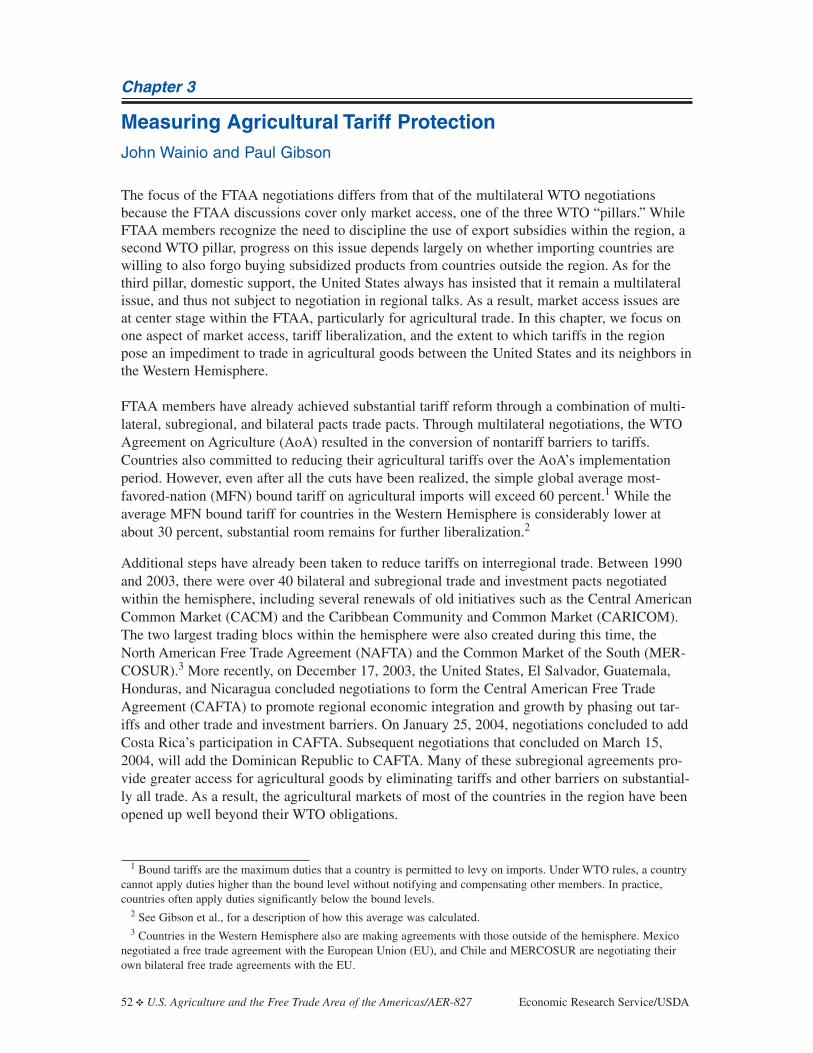
Chapter 3

Measuring Agricultural Tariff Protection John Wainio and Paul Gibson

The focus of the FTAA negotiations differs from that of the multilateral WTO negotiationsbecause the FTAA discussions cover only market access, one of the three WTO “pillars.” WhileFTAA members recognize the need to discipline the use of export subsidies within the region, asecond WTO pillar, progress on this issue depends largely on whether importing countries arewilling to also forgo buying subsidized products from countries outside the region. As for thethird pillar, domestic support, the United States always has insisted that it remain a multilateralissue, and thus not subject to negotiation in regional talks. As a result, market access issues areat center stage within the FTAA, particularly for agricultural trade. In this chapter, we focus onone aspect of market access, tariff liberalization, and the extent to which tariffs in the regionpose an impediment to trade in agricultural goods between the United States and its neighbors inthe Western Hemisphere.

FTAA members have already achieved substantial tariff reform through a combination of multi-lateral, subregional, and bilateral pacts trade pacts. Through multilateral negotiations, the WTOAgreement on Agriculture (AoA) resulted in the conversion of nontariff barriers to tariffs.Countries also committed to reducing their agricultural tariffs over the AoA’s implementationperiod. However, even after all the cuts have been realized, the simple global average most-favored-nation (MFN) bound tariff on agricultural imports will exceed 60 percent.1 While theaverage MFN bound tariff for countries in the Western Hemisphere is considerably lower atabout 30 percent, substantial room remains for further liberalization.2

Additional steps have already been taken to reduce tariffs on interregional trade. Between 1990and 2003, there were over 40 bilateral and subregional trade and investment pacts negotiatedwithin the hemisphere, including several renewals of old initiatives such as the Central AmericanCommon Market (CACM) and the Caribbean Community and Common Market (CARICOM).The two largest trading blocs within the hemisphere were also created during this time, theNorth American Free Trade Agreement (NAFTA) and the Common Market of the South (MER-COSUR).3 More recently, on December 17, 2003, the United States, El Salvador, Guatemala,Honduras, and Nicaragua concluded negotiations to form the Central American Free TradeAgreement (CAFTA) to promote regional economic integration and growth by phasing out tar-iffs and other trade and investment barriers. On January 25, 2004, negotiations concluded to addCosta Rica’s participation in CAFTA. Subsequent negotiations that concluded on March 15,2004, will add the Dominican Republic to CAFTA. Many of these subregional agreements pro-vide greater access for agricultural goods by eliminating tariffs and other barriers on substantial-ly all trade. As a result, the agricultural markets of most of the countries in the region have beenopened up well beyond their WTO obligations.


1 Bound tariffs are the maximum duties that a country is permitted to levy on imports. Under WTO rules, a countrycannot apply duties higher than the bound level without notifying and compensating other members. In practice,countries often apply duties significantly below the bound levels.

2 See Gibson et al., for a description of how this average was calculated.3 Countries in the Western Hemisphere also are making agreements with those outside of the hemisphere. Mexico

negotiated a free trade agreement with the European Union (EU), and Chile and MERCOSUR are negotiating theirown bilateral free trade agreements with the EU.


Another outcome of these pacts is that trade within the region is conducted under an array of dif-ferent tariff rates. Within the United States, agricultural goods imported from some countries mayface MFN tariffs, while the same goods imported from NAFTA countries may face lower tariffrates. In addition, exports of certain agricultural goods from other FTAA countries may be eligi-ble for duty-free treatment under the Generalized System of Preferences (GSP), the CaribbeanBasin Economic Recovery Act (CBERA), or the Andean Trade Preference Act (ATPA). In 2001,more than 60 percent of U.S. agricultural imports from Western Hemisphere countries were eligi-ble to enter at preferential tariff rates, i.e., rates below the MFN bound rates. At the same time,the duties faced by most U.S. exports in its NAFTA partners’ markets are well below MFN levels.In addition, many of the other countries within the hemisphere actually apply duties at rates sub-stantially lower than their permitted MFN bound levels. When trying to gauge the effect that cut-ting MFN tariffs may have on future trade, the large amount that currently takes place at preferen-tial and applied tariffs below bound MFN rates has to be taken into account.

This chapter addresses a number of tariff-related questions relevant to the negotiations: What arethe levels and patterns of tariff protection currently faced by U.S. agricultural exports within theFTAA? To what extent has the United States already opened its agricultural markets to theregion? Which are the most important products being exported by our Western Hemisphere trad-ing partners that continue to face high duties in the United States? Do some products within theregion face higher protection across the board than do others and to what extent are these prod-ucts exported by United States?

Trade and Tariffs Within the FTAA Region

The tariff liberalization that took place within the Western Hemisphere in the 1990s was accom-panied by impressive growth in intraregional trade. During this period, the annual rate of growthin intraregional trade increased by 11.1 percent, exceeding the 8-percent annual growth rate inhemispheric trade with the rest of the world, as well as the annual growth rate in overall globaltrade of 6.6 percent per year (U.S. General Accounting Office, 2001). FTAA agricultural tradebecame an increasingly important component of overall U.S. agricultural trade as well. About 55percent ($23.1 billion) of all U.S. agricultural imports and about 37 percent ($19.9 billion) ofU.S. agricultural exports came from or went to FTAA countries in 2001. NAFTA partnersCanada and Mexico accounted for 38 percent of U.S. agricultural imports and 29 percent of U.S.agricultural exports in 2001. Much of this trade already takes place at zero duties. Comparedwith NAFTA, overall trade with the rest of the FTAA countries is considerably less, accountingfor 17 percent of U.S. agricultural imports and 8 percent of exports. It is this share of U.S. agri-cultural trade that will be most affected by the FTAA. In 2001, the leading U.S. agriculturalexports to FTAA countries consisted of coarse grains, red meats, and snack foods. The leadingimports were fresh vegetables, coffee, and red meats.

Within the region, the United States is generally the most important destination for exports.During the 1998-2000 period, the FTAA countries relied on the U.S. market for an average of 32percent of their agricultural exports, although some marked differences existed between individ-ual countries. The level of dependency on the U.S. market as an export destination was greatestfor the Dominican Republic, which shipped about 80 percent of its total agricultural exportsthere. The NAFTA partners are also highly dependent on the United States, with about 73 per-cent of Mexico’s and 55 percent of Canada’s agricultural exports destined for the United States.The MERCOSUR countries, on the other hand, tend to trade most heavily with each other, ship-ping less than 10 percent of their exports to the United States.4

4 MERCOSUR consists of Argentina, Brazil, Paraguay, and Uruguay.


Table 3-1—Value of U.S. agricultural imports from FTAA countries, 2001, categorized by MFN or non-MFNduty faced1

Total Preferential MFN duty-free MFN with dutiesNumber Number Number Numberof tariff Imports of tariff Imports % of of tariff Imports % of of tariff Imports % of

Exporter lines ($000) lines ($000)2 total lines ($000) total lines ($000) total

Antigua & Barbuda 6 180 3 130 72 3 50 28 0 0 0

Argentina 237 613,194 70 47,898 8 75 186,440 30 109 378,856 62

Bahamas 23 7,219 15 5,692 79 7 814 11 4 713 10

Barbados 25 7,662 17 7,014 92 7 635 8 2 14 0

Belize 34 39,085 27 38,702 99 5 85 0 4 298 1

Bolivia 28 16,473 9 3,380 21 13 12,982 79 8 111 1

Brazil 298 1,008,843 108 114,951 11 107 506,492 50 114 387,400 38

Canada 905 10,448,762 634 7,154,384 68 211 3,231,038 31 303 63,339 1

Chile 207 1,029,063 87 87,745 9 61 385,038 37 89 556,280 54

Colombia 229 944,012 149 369,707 39 60 542,296 57 57 32,009 3

Costa Rica 176 820,078 133 395,319 48 42 423,979 52 17 781 0

Dominica 11 83 8 60 72 2 17 21 1 6 7

Dominican Rep. 212 445,092 159 371,447 83 52 71,735 16 14 1,909 0

Ecuador 189 485,500 126 152,678 31 46 325,872 67 51 6,950 1

El Salvador 113 92,372 76 50,727 55 31 41,227 45 18 418 0

Grenada 7 1,863 5 158 8 2 1,705 92 0 0 0

Guatemala 188 607,914 149 175,730 29 37 431,525 71 15 660 0

Guyana 19 7,468 16 7,181 96 3 276 4 2 11 0

Haiti 23 7,040 13 4,158 59 10 2,864 41 1 18 0

Honduras 103 290,186 72 132,064 46 25 154,106 53 14 4,015 1

Jamaica 130 98,731 86 86,433 88 41 11,006 11 15 1,292 1

Mexico2 619 5,631,860 469 4,643,476 82 151 963,980 17 89 24,404 0

Nicaragua 75 106,727 54 60,066 56 18 46,351 43 9 310 0

Panama 66 41,132 40 25,420 62 20 15,333 37 10 379 1

Paraguay 26 15,927 8 7,009 44 12 8,016 50 8 903 6

Peru 217 213,186 146 130,103 61 59 72,251 34 48 10,831 5

St. Kitts & Nevis 1 72 0 0 0 1 72 100 0 0 0

St. Lucia 5 314 4 286 91 1 28 9 0 0 0

St.Vincent&Gren. 4 133 3 35 26 1 98 74 0 0 0

Suriname 2 295 1 19 6 1 276 94 0 0 0

Trinidad&Tobago 72 17,227 47 13,014 76 23 3,892 23 6 321 2

Uruguay 73 60,353 20 8,010 13 26 8,209 14 27 44,134 73

Venezuela 83 35,174 38 14,861 42 30 18,914 54 21 1,399 4

Total FTAA 1,255 23,093,219 888 14,107,856 61 302 7,467,603 32 549 1,517,761 7

Total NAFTA 1,079 16,080,622 792 11,797,860 73 255 4,195,018 26 339 87,743 1

Total non-NAFTA 831 7,012,598 493 2,309,996 33 213 3,272,584 47 373 1,430,017 20

Global Total 1,516 42,480,933 930 14,920,159 35 393 15,201,018 36 1,056 12,359,756 29 1The definition of agricultural trade corresponds with those tariff lines subject to tariff-cutting committments as specified in Annex 1 of the WTO

Agreement on Agriculture.2All trade entered duty-free with the exception of $2.805 billion of imports from Mexico, which came in at duties that have not yet been cut to

zero under the NAFTA timetable.Sources: U.S. International Trade Commission Trade Dataweb, http://dataweb.usitc.gov; Agricultural Market Access Database,http://www.amad.org


Table 3-1 provides some basic statistics on 2001 U.S. agricultural imports from FTAA countriesas well as the number of tariff-line products in which trade took place.5 Almost 70 percent ofU.S. agricultural imports from the region came from NAFTA partners Canada and Mexico, bothof which tend to have a much broader base in terms of the number of tariff lines and diversity ofproducts exported to the United States. Of the remaining U.S. imports, spread out among theother 31 countries, Chile and Brazil led the way at over $1 billion each, accounting for almost30 percent of the non-NAFTA total.

Table 3-1 also categorizes imports from Western Hemisphere countries by the amount of tradethat came in at MFN versus preferential tariffs. This provides an important gauge of the capacityof the United States to further reduce tariffs under an FTAA as well as an indicator of how muchactual trade will be impacted by tariff cuts.

The U.S. market is already relatively open to the hemisphere. In 2001, 49 percent ($11.3 billion)of total U.S. agricultural imports from FTAA countries entered duty-free under either NAFTA orone of the three nonreciprocal trade preference programs, the GSP, CBERA, and ATPA, each ofwhich offers duty-free entry on a range of products. Another 32 percent ($7.5 billion) of totalagricultural imports entered at MFN duty-free rates. This means that only about 19 percent ofU.S. agricultural imports were assessed duties in 2001. About 12 percent of the total consisted ofimports from Mexico at NAFTA rates that, while not yet duty-free, were considerably belowMFN rates.6 In 2001, only 7 percent ($1.5 billion) of the U.S. imports from FTAA countriescame in at MFN duties. About 4 percent of U.S. imports were assessed MFN duties under 5 per-cent, while less than 1 percent came in at duties above 15 percent.

The larger FTAA countries tend to export a fairly wide range of agricultural products to theUnited States. For many of the smaller countries, however, exports to the United States consistedof only a few products, and often one product dominated. For example, almost 90 percent ofDominica’s exports to the United States during 1998-2000 consisted of cigars, while 87 percentof Grenada’s were made up of nutmeg. In 10 of the 33 countries, a single commodity accountedfor at least one-half of its total exports to the United States.

The value of U.S. duty-free preferences under nonreciprocal trade programs varies across coun-tries, depending on the overall makeup of their agricultural exports. At 99 percent, Belize hadthe highest share of its products enter under preferential rates. A number of Caribbean nations,including the Bahamas, Barbados, the Dominican Republic, Guyana, Jamaica, and St. Luciaexported over 80 percent of their U.S.-bound agricultural products under either GSP or CBERA.Through NAFTA, 68 percent of U.S. agricultural imports from Canada and 82 percent fromMexico benefited from preferential duties. Some countries, however, including Argentina andChile, had extremely low shares (under 10 percent) of their U.S.-bound exports enter at prefer-ential rates.

As a result of preferential rates, the simple unweighted average U.S. applied tariffs facing FTAAcountries in 2001 were even lower. It is generally recognized that U.S. agricultural tariffs are rel-atively low, with an overall simple bound tariff mean of 10.4 percent. Due to NAFTA prefer-ences, Canada at 4.7 percent and Mexico at less than 1 percent face the lowest simple average

5 Product coverage is the same as that specified in Annex 1 of the WTO Agreement on Agriculture. In 2001, theU.S. agricultural tariff schedule distinguished between 1,754 tariff-line items.

6 These duties are being progressively reduced to zero under the NAFTA timetable.

tariffs among FTAA countries.7 Countries qualifying for tariff preferences under the CBERA orATPA programs face simple average tariffs of slightly over 6 percent on agricultural productswhile other FTAA countries, which benefit only from the GSP, face slightly higher averages ofabout 9.1 percent.

While the simple averages may appear to be low, the United States continues to maintain rela-tively high tariffs, with little or no preferential access, on certain agricultural products, many ofwhich are of special export interest to FTAA countries. These include import-sensitive productssuch as sugar and sugar-containing products, peanuts and peanut butter, certain types of tobacco,orange juice, dairy products, and beef. Tariff rate quotas (TRQs) limit imports of many of theseproducts. A TRQ allows a certain amount of a product to be imported at a generally low “inquota” rate, with any additional imports facing the higher “over quota” rate. For example, thetariffs for tobacco imports within the quota are around 10 percent while the tariffs on over-quotaimports are 350 percent.

Table 3-2 shows the extent to which individual FTAA countries’ agricultural exports to theUnited States faced TRQs in 2001. The region as a whole accounted for slightly less than 50percent ($2.0 billion) of the value of products imported under U.S. TRQs, with Canada aloneaccounting for 31 percent ($1.3 billion). The remaining amount was spread over 22 countries,from Brazil ($200,235) to Venezuela ($208). The bulk of this trade took place within the quotaand most of it was at preferential rates. The small amount of over-quota trade was almost exclu-sively from NAFTA partners.8 Neither the GSP, CBERA, nor ATPA program extends preferen-tial access for products subject to over-quota tariffs. That there was very little over-quota trade atMFN rates suggests the trade-chilling effects of these high over-quota tariffs. It also indicatesthat for those FTAA countries whose exports face high over-quota rates, there would appear tobe substantial potential benefit from an elimination of these barriers. A general conclusion fromthese tariff and trade data is that even though the trade benefits for FTAA countries from negoti-ating a free trade agreement with the United States might appear small, given the high propor-tion of trade already taking place at low or zero duties, when one takes into account those sensi-tive products on which prohibitively high rates are levied, the potential benefits could expandconsiderably.

Comparing Tariff Protection Across FTAA Countries

Comparing tariffs across countries is neither a straightforward nor a simple exercise. Over 50years ago, Viner observed that “there is no way in which the ‘height’ of a country’s tariffs as anindex of its restrictive effect can be even approximately measured, or for that matter, evendefined with any degree of significant precision” (Viner, 1950). While there are numerousapproaches to calculate the overall level of tariff protection provided by a country’s tariff sched-ule, none is without some aggregation bias. The easiest and most common approach is to calcu-late a simple unweighted tariff mean. The main drawback with a simple average is that it givesequal weight to all goods regardless of importance in trade.


7 These tariff averages are calculated as simple means across the 1,754 tariff-line items found in the U.S. agricul-tural tariff schedule. Note that tariffs averages calculated from the full tariff schedule differ from those based on 6-digit aggregates of the Harmonized System, as reported in table 3.5

8 Over-quota imports from Mexico were assessed preferential rates under NAFTA, while Canadian imports wouldhave been assessed the MFN rate. All over-quota imports from other countries would also have been at MFN rates.

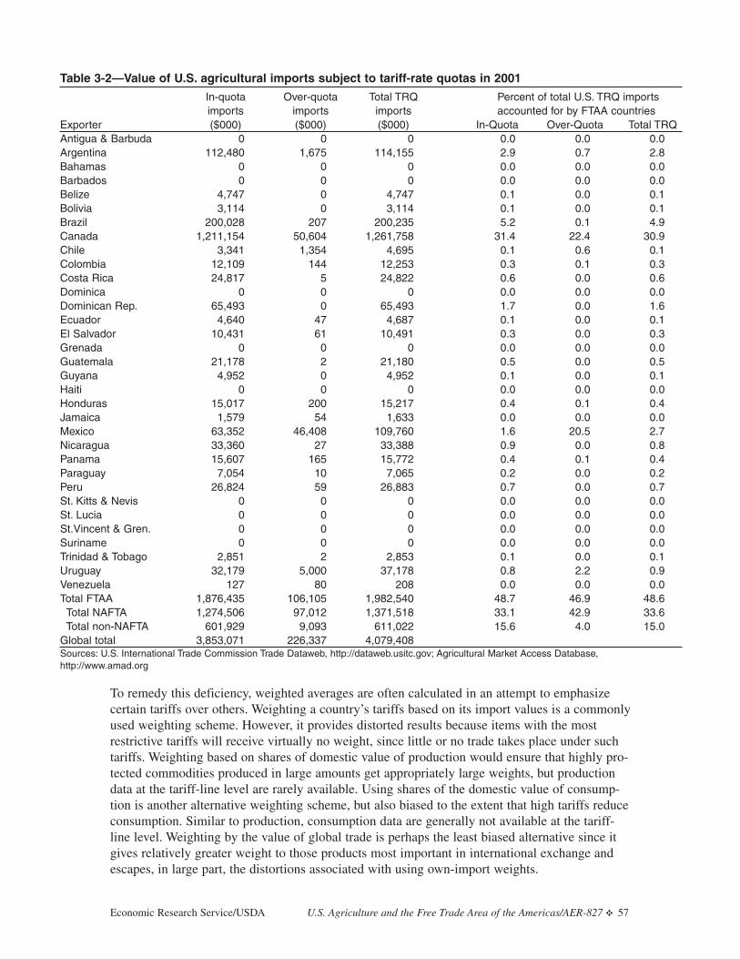
To remedy this deficiency, weighted averages are often calculated in an attempt to emphasizecertain tariffs over others. Weighting a country’s tariffs based on its import values is a commonlyused weighting scheme. However, it provides distorted results because items with the mostrestrictive tariffs will receive virtually no weight, since little or no trade takes place under suchtariffs. Weighting based on shares of domestic value of production would ensure that highly pro-tected commodities produced in large amounts get appropriately large weights, but productiondata at the tariff-line level are rarely available. Using shares of the domestic value of consump-tion is another alternative weighting scheme, but also biased to the extent that high tariffs reduceconsumption. Similar to production, consumption data are generally not available at the tariff-line level. Weighting by the value of global trade is perhaps the least biased alternative since itgives relatively greater weight to those products most important in international exchange andescapes, in large part, the distortions associated with using own-import weights.


Table 3-2—Value of U.S. agricultural imports subject to tariff-rate quotas in 2001

In-quota Over-quota Total TRQ Percent of total U.S. TRQ importsimports imports imports accounted for by FTAA countries

Exporter ($000) ($000) ($000) In-Quota Over-Quota Total TRQAntigua & Barbuda 0 0 0 0.0 0.0 0.0 Argentina 112,480 1,675 114,155 2.9 0.7 2.8 Bahamas 0 0 0 0.0 0.0 0.0 Barbados 0 0 0 0.0 0.0 0.0 Belize 4,747 0 4,747 0.1 0.0 0.1 Bolivia 3,114 0 3,114 0.1 0.0 0.1 Brazil 200,028 207 200,235 5.2 0.1 4.9 Canada 1,211,154 50,604 1,261,758 31.4 22.4 30.9 Chile 3,341 1,354 4,695 0.1 0.6 0.1 Colombia 12,109 144 12,253 0.3 0.1 0.3 Costa Rica 24,817 5 24,822 0.6 0.0 0.6 Dominica 0 0 0 0.0 0.0 0.0 Dominican Rep. 65,493 0 65,493 1.7 0.0 1.6 Ecuador 4,640 47 4,687 0.1 0.0 0.1 El Salvador 10,431 61 10,491 0.3 0.0 0.3 Grenada 0 0 0 0.0 0.0 0.0 Guatemala 21,178 2 21,180 0.5 0.0 0.5 Guyana 4,952 0 4,952 0.1 0.0 0.1 Haiti 0 0 0 0.0 0.0 0.0 Honduras 15,017 200 15,217 0.4 0.1 0.4 Jamaica 1,579 54 1,633 0.0 0.0 0.0 Mexico 63,352 46,408 109,760 1.6 20.5 2.7 Nicaragua 33,360 27 33,388 0.9 0.0 0.8 Panama 15,607 165 15,772 0.4 0.1 0.4 Paraguay 7,054 10 7,065 0.2 0.0 0.2 Peru 26,824 59 26,883 0.7 0.0 0.7 St. Kitts & Nevis 0 0 0 0.0 0.0 0.0 St. Lucia 0 0 0 0.0 0.0 0.0 St.Vincent & Gren. 0 0 0 0.0 0.0 0.0 Suriname 0 0 0 0.0 0.0 0.0 Trinidad & Tobago 2,851 2 2,853 0.1 0.0 0.1 Uruguay 32,179 5,000 37,178 0.8 2.2 0.9 Venezuela 127 80 208 0.0 0.0 0.0 Total FTAA 1,876,435 106,105 1,982,540 48.7 46.9 48.6

Total NAFTA 1,274,506 97,012 1,371,518 33.1 42.9 33.6 Total non-NAFTA 601,929 9,093 611,022 15.6 4.0 15.0

Global total 3,853,071 226,337 4,079,408Sources: U.S. International Trade Commission Trade Dataweb, http://dataweb.usitc.gov; Agricultural Market Access Database,http://www.amad.org


Table 3-3—Top four agricultural exports and concentration ratios - FTAA countries

1998-00 averageexport value Percent

Country Top four HS6-digit export categories $000 of totalAntigua & Barbuda sunflower&safflower oil; peanut oil; raw cane sugar; frsh, chlled

or frzn horsemeat 1,664 46Argentina soymeal; wheat (other than durum ); corn, other than for seed; soybean oil 5,372,464 43Bahamas rum; bananas & plantains; natural sponges; sunflowerseed 152,794 95Barbados raw cane sugar; rum; food preparations, nes; margarine 48,631 72Belize raw cane sugar; bananas & plantains; frozen orange juice; soymeal 112,113 80Bolivia soymeal; soybeans; soybean oil; brazil nuts 291,607 65Brazil soybeans; unroasted coffee; soymeal; raw cane sugar 6,197,053 47Canada wheat (other than durum ); durum wheat; rapeseed; live cattle 4,540,897 28Chile grapes; wine (< 2 lit); fishmeal; apples 1,693,058 48Colombia unroasted coffee; bananas & plantains; cut flowers and buds, fresh;

raw cane sugar 2,542,788 80Costa Rica bananas & plantains; unroasted coffee; pineapples; melons 1,554,500 65Dominica bananas & plantains; cigars & cigarillos; sauces and preparations;

unroasted coffee 19,254 82Dominican Republic cigars & cigarillos; raw cane sugar; cocoa beans; bananas & plantains 390,388 62Ecuador bananas & plantains; cut flowers and buds, fresh; unroasted coffee;

cocoa beans 1,635,083 81El Salvador unroasted coffee; raw cane sugar; food preparations, nes; prepared

cereal products 394,311 69Grenada nutmeg; wheat or meslin flour; mace; cocoa beans 16,676 84Guatemala unroasted coffee; raw cane sugar; bananas & plantains; cardamoms 1,266,949 65Guyana raw cane sugar; rice, husked (brown); rice, broken; rum 141,809 92Haiti unroasted coffee; guavas, mangoes, mangosteens; cocoa beans;

essential oils 21,554 79Honduras unroasted coffee; bananas & plantains; coffee substitutes containing

coffee; cigars & cigarillos 628,844 70Jamaica raw cane sugar; rum; bananas & plantains; unroasted coffee 187,685 56Mexico beer; unroasted coffee; tomatoes, frsh or chlled; spirits (incl.cordials,

liqueurs, & vodka) 2,230,683 30Nicaragua unroasted coffee; raw cane sugar; boneless frsh & chlled beef; shelled

peanuts, unroasted 246,582 58Panama bananas & plantains; raw cane sugar; unroasted coffee; melons 312,689 75Paraguay soybeans; soymeal; cotton (uncarded, uncombed); soybean oil 647,747 75Peru fishmeal; unroasted coffee; asparagus, prepared or preserved,

unfrozen; fish oil 1,184,997 75St. Kitts & Nevis raw cane sugar; mineral & aerated waters; cane molasses;

nonalcoholic beverages 8,147 93St. Lucia bananas & plantains; beer; mineral & aerated waters; peppers 51,716 96St. Vincent

& Grenadines bananas & plantains; wheat or meslin flour; milled rice; roots and tubers 38,226 85Suriname bananas & plantains; rice, husked (brown); unmilled rice; milled rice 31,031 81Trinidad & Tobago rum; mineral & aerated waters; raw cane sugar; cookies & wafers 94,871 42United States soybeans; corn, other than for seed; cigarettes; wheat (other than durum ) 18,092,007 24Uruguay boneless, frozen beef; milled rice; boneless, frsh & chlled beef; cigarettes 460,386 38Venezuela cigarettes; bananas & plantains; unroasted coffee; sesame seeds 188,140 36


Using the value of global trade as a weighting scheme may still not provide countries with theinformation that is needed to evaluate the level of protection their exports face in each importingcountry. Even though two countries’ exports may face exactly the same tariffs in a third country,the average tariff each faces can differ based on the composition of each of the country’sexports. The restrictive effect that an importing country’s tariff schedule has on each of its trad-ing partners’ exports depends on how high its duties are on the basket of products being export-ed by each of these trading partners. Table 3-3 ranks selected FTAA countries based on the per-cent of total agricultural export value accounted for by the top four export categories. The degreeof dependency on a few products is extremely high throughout almost the entire region, with thetop four exports (at the HS 6-digit level) accounting for over 90 percent of total exports in thecases of St. Lucia, the Bahamas, St. Kitts and Nevis, and Guyana.9 All but 10 countries earnover one-half of their agricultural export earnings from only four products. This concentrationlevel demonstrates the importance that a relatively small subset of tariffs can have on tradebetween two partners. Even the United States, which has the most diversified export sector inthe region, does not export every product nor is it equally concerned with every one of its trad-ing partners’ tariffs. The challenge is to devise a meaningful method of measuring and compar-ing relative levels of tariff protection between trading partners that distinguishes between“important” and “unimportant” tariffs.

The information found in tables 3-4 and 3-5 is one way to achieve this goal (see appendix 3-1).Each table contains three sets of tariff means—a simple, unweighted mean of applied tariffs andtwo trade-weighted means, one of applied tariffs and one of bound tariffs.10 Table 3-4 containstariff means faced by U.S. agricultural exports in each of the selected countries, while table 3-5contains the tariff means faced in the United States by each of these countries’ agriculturalexports. The means are based on tariff and trade data at the HS 6-digit level (encompassing 682categories).11 The tables contain 3 sets of tariff means calculated across the 682 categories. Inthe case of the weighted means in table 3-4, the weights used to calculate each mean are basedon global U.S. agricultural exports, not exports to the individual country. In turn, the weightedmeans in table 3-5 are generated using the global agricultural exports of each U.S. trading part-ner as weights. The export-weighting scheme seeks to overcome the usual concern about import-weighting schemes, that high tariffs lead to zero or small imports and thus are underrepresentedin import-weighted averages. Using the exporting country’s total exports as weights ensures thatthe greatest emphasis is placed on those tariffs in the importing country that are of most impor-tance to the exporting partner. It also provides a valuable starting point for considering the effectthat a country’s tariff regime has on its trading partner’s exports.12

From the U.S. perspective, the most protected country in the sample is the Dominican Republic,whether one uses the simple or weighted mean as an indicator. Based on the weighted mean, if

9 The Harmonized System (HS) provides an internationally recognized nomenclature for classifying globally tradedgoods. The World Customs Organization establishes the definitions of HS commodity groupings.

10 All tariff rates were first aggregated in the form of simple averages from the national tariff-line level (usually theHS 8-digit level) to the HS 6-digit level.

11 The U.S. tariff averages found on the previous page were calculated across the 1,754 bound HS-8 tariff-linesfound in the U.S. schedule. The tariff averages found in tables 3-4 and 3-5 were calculated by first calculating simpleaverages for the 682 6-digit levels and then using these averages to calculate the weighted and unweighted overallmeans.

12 See the appendix to this chapter for a detailed discussion of the export-weighting methodology. Like otherweighting schemes, export weights have some limitations. Differences in the composition of a country’s bilateraltrade flows may result from differences in its trader partners’ consumer preferences or from policies such as historicalquota rights, rather than the partners’ tariffs.


Table 3-4—Tariff averages faced by United States in selected FTAA countries

Applied rates Simple MFN bound ratesweighted by unweighted weighted byU.S.exports MFN applied U.S.exports

at the HS6 level rates (HS6) at the HS6 levelArgentina 12.7 12.9 34.9Brazil 12.7 12.7 40.0Canada 1 7.0 6.1 12.8Chile 9.0 9.0 25.0Colombia 15.0 14.8 104.3Costa Rica 13.0 11.5 35.7Dom Rep 18.5 21.4 40.0Ecuador 14.0 14.3 26.7El Salvador 9.6 10.3 43.4Guatemala 9.4 9.2 54.7Haiti 16.0 16.0 16.0Honduras 12.1 11.0 35.0Jamaica 16.1 17.7 100.0Mexico 1 8.6 2.9 51.8Nicaragua 8.0 7.0 59.5Panama 12.4 12.5 27.8Paraguay 12.1 12.6 34.9Peru 16.9 17.2 30.0Uruguay 12.5 12.7 36.8Venezuela 15.0 14.8 56.21Applied rates in the case of Canada and Mexico are the 2001 NAFTA rates.

Table 3-5—Tariff averages facing FTAA exports to the United States

U.S. MFNbound

U.S. applied rates1 ratesMean Simple weighted

weighted by unweighted by totaltotal exports mean exports

Argentina 6.1 3.9 6.5Brazil 12.8 3.9 13.6Canada 1.2 1.2 4.2Chile 2.1 3.9 2.7Colombia 2.2 1.8 3.9Costa Rica 1.1 1.8 3.8Dom Rep 8.9 1.8 13.4Ecuador 0.6 1.8 2.0El Salvador 5.1 1.8 6.7Guatemala 6.3 1.8 8.4Haiti 0.1 1.8 3.0Honduras 1.1 1.8 3.4Jamaica 10.3 1.8 15.5Mexico 0.8 0.4 5.5Nicaragua 8.4 1.8 10.6Panama 3.0 1.8 5.0Paraguay 4.2 3.9 4.4Peru 0.5 1.8 2.7Uruguay 6.1 3.9 7.4Venezuela 7.0 3.9 8.71Applied rates include tariff preferences extended under nonreciprocal tariff preference programs (GSP, CBERA, andATPA). In the case of Canada and Mexico they are the 2001 NAFTA rates.

all U.S. agricultural exports had gone to the Dominican Republic during the base period, theaverage duty faced would be about 18.5 percent. This average is due to tariffs of 30 percent orhigher on such important U.S. exports as tobacco products, pet foods, almonds, apples, andbaked goods. These tariffs are assigned relatively heavy weights in the calculations. Peru had thesecond highest tariff protection on U.S. agricultural exports due to fairly high (25-30 percent)rates on meats and grains, other important U.S. exports. On the other end of the spectrum, fivecountries—Canada, Nicaragua, Mexico, Chile, and Guatemala—all have weighted tariff meansof less than 10 percent.

U.S. exports face applied tariffs in Western Hemisphere markets that are considerably lower thanthe bound rates. The lowest applied rates tend to be concentrated in products of use to farmers(seeds, cuttings and live plants, semen, breeding stock, etc.) or plant and animal materials withcommercial uses (gums, resins, essential oils, extracts, and hides and skins). Regional trade inmany of these products is fairly modest. However, some products that are very important to U.S.agriculture, including wheat, soybeans, and cotton, also face low applied tariffs in many,although not all, countries within the hemisphere. It is also the case, however, that many prod-ucts face uniformly higher-than-average tariffs within the region. From the standpoint of U.S.exports, the most important of these are tobacco products, meats, rice, beer, wine, and distilledspirits. Certain fruits and vegetables including apples, grapes, oranges, grapefruit, potatoes, andonions also face higher-than-average applied tariffs in many markets especially during specifictimes of the year when domestic production is available. Finally, dairy products, sugar, andprocessed products containing dairy products and sugar tend to face higher-than-average appliedtariffs in most countries.

Comparing the weighted and simple unweighted applied means of each country gives a goodindication of the level of bias each country’s tariff schedule contains against U.S. exports. To theextent that a country levies higher tariffs on those products that are important from a U.S. exportperspective than on those products not important to the U.S., the weighted average will exceedthe unweighted one. In this respect, Mexico’s tariff schedule demonstrates the highest relativebias against U.S. exports. When weighted by U.S. exports, Mexico’s mean applied tariff isalmost three times the simple unweighted mean. This is understandable, however, since underNAFTA tariffs on some products were immediately cut to zero while others were reduced tozero by the end of 2003. In the case of the most import-sensitive commodities, however, tariffswill not reach zero until 2008. In 2001, Mexico was still levying tariffs on several importantU.S. export commodities, including corn, poultry, and tobacco/tobacco products. In general,however, there is not much difference between the weighted and unweighted tariff means intable 3-4 partly because countries within the hemisphere tend to have relatively low levels ofdispersion across both their bound and applied tariffs.

The overall, export-weighted, average applied rate for the countries found in table 3-4 is 12.5percent, less than one-third of the bound average of 43.3 percent. The difference between theapplied rates that U.S. exports face and the bound rates are especially large for Jamaica,Nicaragua, and Colombia. Mexico also shows a large difference, with U.S. agricultural exportsfacing an export-weighted, average NAFTA tariff in Mexico of 8.6 percent versus an averagebound tariff of over 50 percent. This is an indication of the maximum level of protection thatU.S. exports could have faced if NAFTA did not exist and if Mexico applied tariffs at the boundlevels. But, Mexico also tends to apply tariffs at levels below the MFN bound rates. Thus, amore accurate indication of the impact of NAFTA would be to compare the NAFTA averagewith an export-weighted average of Mexico’s applied tariffs. If NAFTA were not in place, U.S.exports would have faced an export-weighted, average MFN applied tariff in Mexico of 35.4percent versus the NAFTA average of 8.6 percent. In the case of Canada, the only other market


in the hemisphere where the United States received preferential treatment in 2001, the MFNapplied and bound rates are the same. Thus, in the absence of NAFTA, U.S. exports would havefaced a weighted MFN bound rate of 12.8 percent in Canada instead of the lower NAFTA aver-age of about 7 percent.

Table 3-5 reports the tariffs that each of the 20 FTAA countries faces in the U.S. market. Thefirst two columns contain the unweighted and weighted means of U.S. applied tariffs, which candiffer by exporter based on eligibility for tariff preferences under either NAFTA or one of thenonreciprocal tariff preference programs GSP, CBERA, or ATPA. Again, we provide a weightedaverage of bound tariffs for comparison purposes.

Given the mix of agricultural products it exports globally, Brazil, at 12.8 percent, faces the high-est export-weighted duties in the United States. The United States levies relatively high tariffs ona number of Brazil’s important exports, including sugar, orange juice, tobacco, and soybean oil.Jamaica was the only other country facing an export- weighted average tariff of over 10 percent,largely a function of the importance of its sugar exports, which make up over one-quarter oftotal exports. On the other end, the exports of four countries—Haiti, Peru, Ecuador, andMexico—all faced average tariff rates below 1 percent in the U.S. market. The top exports fromeach of these countries tend to face very low or zero duties in the United States. In fact, for theregion as a whole (excluding NAFTA partners) the top four exports are coffee, bananas,soymeal, and soybeans, all of which face low or zero duties.

Even though the averages are low, the export-weighted applied rates exceed the unweighted onesin all but six of the countries, and in some cases they are over three times as large. Is this anindication that the U.S. tariff schedule is biased against the exports of most FTAA countries?The answer is more complicated than it appears, because of the size and importance of the U.S.market and the structure of the U.S. tariff schedule. In the previous section, we demonstratedthat the U.S. market is already relatively open to agricultural trade within the hemisphere, fortwo reasons. First, the United States has bound 22 percent of its agricultural tariffs at zero in theWTO, and most of the remaining rates have been bound at low levels. As a result, the UnitedStates has the lowest simple mean bound tariff in the region. Additionally, under the CBERAand the ATPA programs, eligible countries are granted duty-free access on their exports to theUnited States. The two programs extended duty-free access to about 65 percent of all agricultur-al tariff lines in the U.S. tariff schedule. With a total of 87 percent of all agricultural tariff-linesbeing duty-free, it is not surprising that CBERA and ATPA countries face simple applied tariffaverages of only 1.8 percent.13 However, these low averages conceal a number of relatively hightariff peaks, many of which are found on products of export interest to some FTAA countries,including sugar, tobacco, frozen orange juice, soybean oil, and peanuts. When these tariffs areweighted by each country’s exports, the weighted averages tend to exceed the unweighted ones.

For some countries in the hemisphere, the differences in the weighted and unweighted averagesdemonstrate that there are considerable potential trade benefits from reducing U.S. tariffs. Thisconclusion would not have been evident based solely on the low simple average tariffs thesecountries face. For some of these, however, market access is being provided through tariff-ratequotas. This can skew the weighted tariff averages found in table 3.5. Sugar, the fifth most


13 The simple averages reported in the previous section are higher than those reported above because they are anaverage over all 1,754 HS 8-digit tariff-lines in the U.S. schedule. In this section, we first calculated simple averagesat the HS 6-digit level. This collapsed the tariff database to 682 HS 6-digit tariffs. This allowed us to use each coun-try’s exports, which are only available at the HS 6-digit level, as weights.

important export from FTAA countries is a good example, since it faces high average duties inthe United States, as a result of steep over-quota tariffs. For almost one-half of the countries intable 3-5, U.S. sugar tariffs are the largest component of the weighted average (see table 3-3).The high weight accorded to sugar in our calculations is potentially misleading in the case ofthose countries whose sugar exports are largely a result of the quota allocation they receiveunder the U.S. sugar TRQ. This is particularly true of some Caribbean countries, where thequota allotment they receive is equal to more than one-half of their total exports to the world.Some of these countries are actually net importers of sugar, and it is likely that the value of theirsugar exports would be significantly less were they not guaranteed a high price on their within-quota exports to the United States. When countries are allocated part of a lucrative quota, theresult might be to create a trade flow that might otherwise not have taken place under free trade.

Comparing the preferential and MFN bound tariff averages is also revealing. In percentage pointterms, the differences are perhaps not as great as one might expect, especially in view of theextension of duty-free access on 65 percent of all tariff-lines under the CBERA and ATPA pro-grams. However, most of the eligible products under these programs already face low duties. Infact, the simple average tariff across those lines on which preferences are extended is about 7 per-cent, while the simple average of the remaining 13 percent of dutiable tariffs on which no prefer-ences are extended is about 47 percent. The conclusion here is that the GSP, CBERA, and ATPAhave not significantly diluted the potential value of an FTAA to the region. There are still manyproducts of export interest to our regional trading partners that do not receive preferences underU.S. programs. In addition, just as U.S. trading partners in the region can legally raise theirapplied rates to their bound levels, the United States can always withdraw or modify the preferen-tial access it gives under these programs. This should provide these countries an incentive to lockin duty-free access to the U.S. market through a reciprocal agreement like the FTAA.


Figure 3-1Relative tariff ratio indices1

1.01.51.61.92.12.12.12.1

4.12.9

4.35.9

6.710.710.7

11.824.3

32.8

0.9

126.6

0 5 10 15 20 25 30 35 40

HaitiPeruEcuadorCosta RicaHondurasMexicoColombiaCanadaChilePanamaParaguayVenezuelaArgentinaDom RepUruguayEl SalvadorJamaicaGuatemalaBrazilNicaragua

1 Ratio of weighted tariff mean faced by U.S. exports in selected countries over weighted tariff mean faced by that country’s exports in the United States.

Sources: U.S. International Trade Commission Trade Dataweb, http://dataweb.usitc.gov; USDA-ERS International Bilateral Agricultural Trade Database (compiled from the U.N. COMTRADE database).

To give expression to the relative importance of two trading partners’ tariffs, Sandrey utilizes thesort of information found in tables 3-4 and 3-5 to create a tariff- and trade-based measure calledthe Relative Tariff Ratio Index (RTR).14 The RTR is a useful way to combine the trade and tar-iffs of two trading partners into a single and concise figure. Figure 3-1 contains RTRs calculatedas the ratio of the trade-weighted average tariff that U.S. exports face in the selected countriesfrom table 3-4 (the numerator) and the equivalent average faced by their exports in the UnitedStates from table 3-5 (the denominator). A ratio of one would reflect similar protection in therespective tariff schedules of the two trading partners. A ratio greater than one means that U.S.agricultural exports face higher average tariffs in the trading partner’s market than its exportsface in the U.S. market. RTRs range from well over 100 for Haiti and to below 1 for Nicaragua(fig. 3-1). These ratios do not reflect the levels of tariffs, but rather the relative tariff protectionfaced at the respective borders of bilateral trading partners. In the case of Haiti, for every tariffpercentage point, on average, that Haitian agricultural exports face in the United States, theUnited States faces 126.6 percentage points in Haiti. In 6 of the 20 countries surveyed, U.S.agricultural exports face average tariffs more than 10 times as high as their exports face in theUnited States. Nicaragua is the only country in which the tariffs faced by U.S. exports are lessthan those faced in the United States by its trading partner’s exports.

Conclusion

Through a combination of multilateral, intraregional, and bilateral pacts, Western Hemispherecountries have made significant progress in reducing agricultural tariff protection over the lastdecade. In an effort to build on the trade and investment ties created by these pacts, 34 countriesin the hemisphere resolved to form a FTAA. One of the main goals of the FTAA is to progres-sively eliminate tariffs on substantially all trade within the hemisphere.

It is in the interest of all Western Hemisphere countries to reduce tariff protection in order toobtain cheaper sources of supply and to achieve the increased level of economic activity madepossible by a more efficient utilization of resources. Free trade permits these efficiency gains byallowing greater specialization according to each country’s “comparative advantage.” Trade lib-eralization will make possible important economic benefits such as greater exploitation ofeconomies of scale and increased domestic and foreign investment in response to new exportopportunities. An FTAA would stimulate the U.S. agricultural economy by reducing the hightariff barriers on U.S. agricultural exports to the region. U.S. agricultural exports face weightedaverage tariffs within the largest non-NAFTA markets in the region that range from just under10 percent to almost 20 percent. The bound rates that these countries committed to in the WTOare even higher, with the weighted averages ranging from 16 percent to over 100 percent. Theextent of the gains from increased trade to the United States depends not just on the level ofapplied tariffs to its exports but also on what these barriers might be in the future if no FTAAwere established. There is always the possibility that these countries could raise their appliedrates to the much higher bound levels.

Over the past decade, Western Hemisphere countries have actively pursued liberalizing and inte-grating their economies through a wide variety of interregional free trade and customs unionagreements. The United States currently has negotiated free trade agreements with nine coun-tries in the region: Canada and Mexico through NAFTA, the five Central American countries


14 Sandrey attributes the original concept for the RTR to John Luxton, former Associate Minister for Foreign Affairsand Trade in New Zealand. See appendix for more information on the RTR.


plus the Dominica Republic through CAFTA, and Chile through the U.S.-Chile FTA. In theremaining countries in the hemisphere U.S. exporters often compete with other countries in theregion whose exports are subject to considerably lower duties. From the U.S. perspective, astrong argument in favor of an FTAA is that it would eliminate the disadvantage U.S. exportersconfront when competing with exports from countries facing preferential rates, thus enablingthem to expand market share.

Opening hemispheric markets has presented negotiators with a number of challenging issues,including reaching agreement on which tariff rates to use as a starting point, how quickly tophase in the elimination of tariffs, and how to treat sensitive products (those most vulnerable toimport competition). Negotiators have agreed to use tariffs that were actually being applied inOctober 2002 as the base rates from which cuts will be made (Spitzer, 2003).15 Starting the cutsfrom applied tariffs is important for U.S. exports since our analysis shows that the weighted-average bound tariffs facing U.S. exports are on average 3.5 times higher than applied tariffs.Therefore, progressively eliminating tariffs from their bound levels would mean that significanttrade liberalization for some U.S. products might not begin until the end of the implementationperiod. By agreeing to use the applied rates as the starting point, U.S. exporters will gainincreased market access within the first year of the agreement.

Negotiators also have established four elimination categories: category A tariffs are to be elimi-nated immediately; category B in the short term (up to 5 years); category C in the medium-term(up to 10 years); and category D in the long term (longer than 10 years) for a limited number ofthe most sensitive commodities. To date, there has been no definitive agreement on the extent towhich countries will be able to place sensitive agricultural products into category D, but accord-ing to the WTO rules governing the formation of FTAs, tariffs must be eliminated on substan-tially all products within 10 years after the agreement’s initial implementation date.

This analysis has focused on one aspect of market access—tariff liberalization—and the extentto which tariffs in the region pose an impediment to trade in agricultural goods between theUnited States and its trading partners in the hemisphere. Using an index that combines tradeflows and tariffs into one simple measure has allowed us to compare the levels of tariff protec-tion that U.S. exports face in other countries with the average levels faced by those countries inthe U.S. market. Using a country’s trading partner’s total exports as weights allows us to escape,in large part, the distorting effects that high tariffs have on the country’s imports. This approachcould provide a useful aggregate measure to compare how an individual country’s allocation ofproducts across categories with different tariff elimination timetables might affect the export bar-riers that it faces over the course of the implementation period.

While we cannot formally project the potential FTAA-induced expansion in U.S. agriculturalexports in this analysis, our detailed comparison of the levels of trade and tariff protection with-in the region shows that there would be considerable potential benefits to the United States fromfurther trade liberalization within the hemisphere. The average level of tariff protection in thesecountries is considerably higher than in the United States. As a result, an FTAA would requirelarger cuts in FTAA country tariffs than in U.S. ones. However, it does not necessarily followthat after all adjustments have had time to take place, we would see a significant imbalance intrade gains. Even in the short term, countries that export a large share of products such as sugar,peanuts, tobacco, and orange juice, on which protection is generally higher in the United States,

15 An exception has been granted for the CARICOM countries, which will be allowed to start their reductions fromWTO bound rates for some agricultural products.

are likely to benefit. In the longer term, because of its size and wealth, the U.S. market shouldprovide ample incentive for countries currently protected by high tariffs to restructure theirindustries in order to compete with U.S. producers. Indeed, one of the main incentives for LatinAmerican countries to form an FTAA is to attract the investment that would allow them to even-tually diversify and expand their exports.

References

Erzan, Refik, and Alexander Yeats. Free Trade Agreements with the United States—What’s In Itfor Latin America? WPS 827, The World Bank, January 1992.

Gibson, Paul, John Wainio, Daniel Whitley, and Mary Bohman. Profiles of Tariffs in GlobalAgricultural Markets. Agricultural Economic Report No. 796, U.S. Department of Agriculture,Economic Research Service, January 2001.

Sandrey, Ron. The Relative Tariff Ratio Index. New Zealand Trade Consortium Working PaperNo. 7. The New Zealand Trade Consortium with the New Zealand Institute of EconomicResearch, 2000.

Spitzer, Robert J. Progress in the FTAA Negotiations. Paper presented at AgriculturalCompetitiveness and World Trade Liberalization conference. Fargo, ND. May 29-30, 2003.

U.S. General Accounting Office, Free Trade Area of the Americas – Negotiators Move TowardAgreement That Will Have Benefits, Costs to U.S. Economy. GAO-01-1027, September 2001.

Viner, Jacob. The Customs Union Issue. Carnegie Endowment for International Peace. NewYork, 1950.

Wainio, John and Paul Gibson. U.S. Exports Face High Tariffs in Some Key Markets.FoodReview, Vol.4, Issue 3, U.S. Department of Agriculture, Economic Research Service,September-December 2001.

Winters, L. Alan. “Reciprocity” chapter. The Uruguay Round—A Handbook on the MultilateralTrade Negotiations. J. Michael Finger and Andrzej Olechowski, editors. The World Bank,Washington, DC., 1987.


Chapter 4

U.S. Sugar in the FTAAStephen Haley

The consequences of a Free Trade Area of the Americas (FTAA) for the supply, distribution, andpricing of U.S. sugar are not yet known. Several scenarios of increased market access to the U.S.sugar market under the FTAA are possible, each with different effects on domestic sugar produc-ers, consumers, and U.S. sugar policy.

Using the U.S. Department of Agriculture (USDA) sugar projections baseline model to analyzethe effects of several market access options, this chapter looks first at the cost structures ofWestern Hemisphere sugar-producing sectors. The ability of Western Hemisphere sugar-produc-ing countries to supply the U.S. market is discussed, with the assumption that FTAA outcomeswill be consistent with current U.S. international commitments affecting sugar. The overallanalysis is being done in the context of domestic sugar policy, with consideration of how somepolicy instruments may be used to adjust to increased sugar access from the hemisphere.

Costs of Sugar Production

One way of analyzing the competitiveness of sugar-producing countries in the WesternHemisphere is to compare and rank average costs of their production. LMC International period-ically publishes estimates of world sugar and sweetener costs of production.1 The data go backto 1979/1980 and The 2000 Report extends the data through 1998/99. Field, factory, and admin-istrative costs are examined for 41 countries that produce sugar from sugar beets and for 63countries that produce sugar from sugarcane. All sugar-producing countries in the WesternHemisphere are included. Although there are many limitations in the use of production cost esti-mates, these data can form the basis for comparing competitiveness in production across regionsand countries.2

Table 4-1 shows four groupings of Western Hemisphere sugar-producing countries rankedaccording to average costs of producing raw cane sugar during 1994/95-1998/99. (Figure 4-1shows the same information as a cumulative cost curve for the individual countries.) The lowestcost producers are in Center/South Brazil, Colombia, El Salvador, and Guatemala. Together,these countries’ sugar production averaged about 14.8 million metric tons (mt) or about 48 per-cent of total hemispheric production. The average cost was estimated at a very low 7.7 cents apound. The second grouping includes Bolivia, North/East Brazil, Costa Rica, Ecuador, Mexico,Nicaragua, and Florida in the United States. Production costs averaged 12.34 cents a pound, andaverage production averaged slightly less than 10.0 million mt. Together, the first and secondcost groupings constitute more than 80 percent of cane sugar production in the WesternHemisphere, giving the cumulative cost curve a long portion below or close to the weighted-average hemispheric cost (100 in fig. 4-1).


1 The study is copyrighted. Results for specific countries or regions may not be quoted or published without theprior approval of LMC International. For more detailed information regarding LMC services, contact: Andrea Kavaler,LMC International, 1841 Broadway, New York, NY, 10023, or by telephone at (212) 586-2427, or via e-mail at:[email protected].

2 See “U.S. and World Sugar and HFCS Production Costs, 1994/95-1998/99,” in Sugar and Sweetener Situation andOutlook, USDA-ERS, SSS-232, September 2001, http://www.ers.usda.gov/publications/so/view.asp?f=specialty/sss-bb/.


The third grouping includes Argentina, Belize, Guyana, Honduras, Panama, Paraguay, Peru, andLouisiana and Texas in the United States. Production costs averaged 16.54 cents a pound. Thefourth group takes into account the highest cost areas, which includes Hawaii in the UnitedStates. The third and fourth groupings’ production averaged 4.1 and 1.9 million mt, respectively.These third and fourth groupings represent the more nearly vertical shaping of the cost curve forcumulative production above 25 million mt (fig. 4-1).

Table 4-1—Costs of producing raw cane sugar, select categories of Western Hemisphereproducers, 1994/95-1998/99

Category Low High AverageCents/pound1

Low cost2 6.72 11.69 7.70Low-to-medium cost3 10.58 17.40 12.34Medium-to-high cost4 14.25 21.83 16.54High cost5 17.74 40.21 23.561Measured in current U.S. cents per pound, ex-mill, factory basis.2Low-cost group is comprised of Center/South Brazil, Colombia, El Salvador, and Guatemala.3Low-to-medium cost group is comprised of Bolivia, North/East Brazil, Costa Rica, Ecuador, Mexico (Gulf and PacificCoasts), Nicaragua, and Florida.4Medium-to-high cost group is comprised of Argentina, Belize, Guyana, Honduras, Panama, Paraguay, Peru, Louisiana,Texas.5High Cost group is comprised of Barbados, Dominican Republic, Jamaica, St. Kitts, Trinidad, Hawaii, Uruguay, andVenezuela.Source: LMC International, 2000.

Figure 4-1 Cumulative cane sugar costs in the Western Hemisphere,relative to weighted-average costs, 1994/95-1998/99

0

50

100

150

200

250

300

0 5,000 10,000 15,000 20,000 25,000 30,000 35,000

1,000 metric tons

Per

cent

age

Production Costs (LMC International)

These data show U.S. cane sugar-producing areas in Louisiana, Texas, and Hawaii in the highercost categories. This means that at least 80 percent of cane sugar production in the hemisphereoccurs at lower cost than in these areas.

The United States is the only significant producer of beet sugar in the Western Hemisphere.Although LMC International ranks the United States as one of the world’s lowest cost producersof beet sugar, its costs in aggregate are still high relative to other Western Hemisphere cane sugarproducers. Table 4-2 shows a low to high range of U.S. production costs, white sugar basis, forcane and beet sugar. The ranges are essentially overlapping in the United States, but the Westernbeet sugar producing areas generally have higher average costs than do those in the East.

Figure 4-2 shows U.S. cane and beet sugar-producing regions’ disaggregated field and factorycosts as percentages of hemispheric averages. Only Florida has a cost element (factory costs)lower than the average. Field and factory costs in U.S. cane areas other than Florida are any-where from 37 percent to 90 percent higher than the corresponding hemispheric average. TheEastern U.S. beet sugar costs are about 16 percent higher than in Florida. The Western U.S. beetsugar costs are intermediate between Texas and Hawaii.


Table 4-2—Range of costs of producing raw cane sugar, and refined beet sugar in theUnited States, 1994/95-1998/99

Category Low HighCents/pound1

Cane sugar, white value equivalent 14.91 27.88

Beet sugar, Eastern U.S. 15.27 25.13Beet sugar, Western U.S. 19.25 34.061Measured in current U.S. cents per pound, ex-mill, factory basis.Source: LMC International, 2000.

Figure 4-2 U.S. sugar costs as percentage of Western Hemisphere average, 1994/95-1998/99

0

20

40

60

80

100

120

140

160

180

200

Florida Eastern U.S.Beet

Louisiana Texas Western U.S.Beet

Hawaii

Costs: raw basisSource: LMC International, 2000.

Per

cent

age

Field Factory

Net Surplus Production

Many factors influence the direction and magnitude of trade flows. Although cost considerationsare important for assessing competitiveness, they are not sufficient for predicting trade flows.Factor endowments, marketing infrastructure, investment capital, industrial organization, con-sumer preferences, government policies, and other elements are important. These elements, how-ever, are not analyzed here in depth because this report’s focus emphasizes the implications ofincreased access of Western Hemisphere sugar on U.S. sugar supply, use, and prices.

Consideration of hemispheric costs shows the United States to be a relatively high-cost sugarproducer, although there are U.S. producing regions where costs are competitive with cost-effi-cient hemispheric producers. Equally important for analysis is consideration of existing tradepatterns and the likelihood that sugar produced in the Western Hemisphere could be shipped intothe U.S. market. A simple way to approach this issue is to examine the net surplus productionstatus of individual countries. Although there are alternative ways to define net producer status,the one chosen in this chapter is the difference of average production less average consumptionfor 1995/96-1999/2000. The averaging approach reduces the effects of extraordinary events andstock-level changes.

Table 4-3 shows net surplus production data for all countries, with totals reported for the geo-graphical groupings of North America, the Caribbean, Central America, and South America. Thehemisphere as a whole is a large net surplus producer of sugar—more than 8.4 million mt. Netsurplus production is positive in all areas except North America where the U.S. and Canadiandeficits outweigh Mexico’s positive balance by more than 2.0 million mt. The ratio of net sur-plus production to production is sizeable in the three surplus areas: 57.1 percent in CentralAmerica, 36.2 percent in South America, and 32.9 percent in the Caribbean. Most countries inthose areas are very experienced in the international market.

The South American and Central American countries tend to have lower costs of production cou-pled with relatively large net production surpluses. A combination of low production costs andlarge net surpluses would indicate a high capability of directing more exports to the U.S. market,although marketing costs would have to be considered as well. The Caribbean area, on the otherhand, is fairly high cost. Most of their exports go to the European Union and the United Statesunder preferential arrangements that guarantee them prices much higher than world levels, there-by covering, to a greater extent than otherwise, their high costs of production. It is only in thisarea where additional trade directed to the U.S. market might seem questionable.

U.S. Sugar Policy

In 1998 at the San Jose Ministerial meeting, the United States and other Western Hemispherecountries agreed that any FTAA agreement will be consistent with the rules and disciplines of theWorld Trade Organization (WTO) and that the FTAA will have to coexist with subregional agree-ments, such as the North American Free Trade Agreement (NAFTA). In addition, it seems reason-able that the U.S. Government is likely to continue its price support for U.S.-produced sugar.

U.S. sugar policy contains three elements: (1) WTO obligations, especially minimum access onimports of raw and refined sugar; (2) NAFTA obligations governing imports of sugar fromMexico; and (3) the U.S. sugar program. Descriptions of these elements follow.


U.S. Sugar Imports and the World Trade Organization

As part of the Uruguay Round Agreement on Agriculture (URAA), the United States agreed toimport a minimum quantity of 1.256 million short tons, raw value (STRV) of raw and refinedsugar each marketing year (October/September). Included in this amount is a commitment toimport at least 24,251 STRV of refined sugar. The URAA made these commitments bindingunder the WTO.


Table 4-3—Average sugar production and consumption, 1995/95-1999/2000

Net surplusDomestic production

Region/Country Production consumption of sugarNorth America

Canada 128 1,230 (1,102)Mexico 4,989 4,300 689 United States 7,260 8,913 (1,653)

Total 12,377 14,443 (2,066)

CaribbeanBarbados 58 17 42 Dominican Republic 514 305 210 Haiti 10 84 (74)Jamaica 215 125 89 St. Kitts and Nevis 21 4 17 Trinidad and Tobago 103 84 19

Total 922 619 303

Central AmericaBelize 113 14 99 Costa Rica 361 205 156 El Salvador 418 219 200 Guatemala 1,560 438 1,121 Honduras 250 224 26 Nicaragua 349 181 168 Panama 168 99 69

Total 3,219 1,380 1,839

South AmericaArgentina 1,644 1,421 223 Bolivia 295 228 67 Brazil 16,490 8,720 7,770 Chile 495 691 (196)Colombia 2,155 1,333 821

Ecuador 356 390 (34)Guyana 271 32 239 Paraguay 125 115 11 Peru 617 896 (279)Surinam 1 14 (13)Uruguay 20 110 (90)Venezuela 580 752 (172)Total 23,049 14,702 8,347

Grand Total 39,567 31,144 8,423Source: USDA

The raw cane sugar tariff-rate quota (TRQ) is allocated to 40 quota-holding countries based on arepresentative period (1975-1981) when trade was relatively unrestricted. A duty of 0.625 cent apound, raw value, is applied to in-quota imports.3 Most countries have the low duty waivedunder the General System of Preferences or the Caribbean Basin Initiative. Between 95 and 98percent of the raw cane sugar TRQ fills each year, and the refined sugar TRQ is filled almost assoon as it opens.

The high-tier sugar tariff applies to sugar imports above the level of the sugar TRQ. TheUruguay Round specified base rates for raw cane sugar of 18.08 cents a pound and for refinedsugar of 19.08 cents a pound. Starting in 1995, the rates were to be cut by 0.45 cent a poundeach year for raw sugar and 0.48 cent a pound for refined sugar. The yearly reductions were totake place until 2000, when the raw sugar high-tier tariff was to be 15.36 cents a pound and therefined sugar high-tier tariff rate was to be 16.21 cents a pound.

North American Free Trade Agreement

The North American Free Trade Agreement (NAFTA) contained provisions on trade in sugar.Those provisions were modified by a side letter in November 1993, before NAFTA went intoeffect on January 1, 1994.

According to the NAFTA side letter, Mexican sugar low-tier tariff exports to the United Statesare restricted by Mexico’s net surplus production of sugar. The “net surplus” is defined asMexico’s production of sugar less its consumption of sugar and high-fructose corn syrup. FromFY 2001 through FY 2007, Mexico is to have duty-free access to the U.S. market for the amountof its surplus as measured by the formula, up to a maximum of 250,000 metric tons, raw value(MTRV). Beginning in FY 2008, Mexico is to have duty-free access with no quantitative limit.

NAFTA specifies a declining high-tier tariff schedule for raw and refined sugar over the transi-tion period to duty-free sugar trade in 2008. For 2003, the raw sugar tariff was 7.56 cents apound, and the refined sugar tariff was 8.01 cents a pound. The raw sugar tariff is scheduled todrop about 1.5 cents each year, and the refined sugar tariff about 1.6 cents a year. Both rates willthen reach zero in FY 2008.

Sugar Loan Program, Allotments, and Payment-in-Kind Acreage Diversion

The primary policy tools available to the U.S. Department of Agriculture to assist sugarcane andsugar beet producers are contained in the Farm Security and Rural Investment Act of 2002 (the2002 Farm Act). The U.S. sugar program provides for USDA to make loans available to proces-sors of domestically grown sugarcane at a rate of 18 cents per pound and to processors ofdomestically grown sugarbeets at the rate of 22.9 cents per pound for refined sugar. Loans aretaken for a maximum term of 9 months and must be liquidated along with interest charges bythe end of the fiscal year in which the loan was made. The loans are nonrecourse. This meansthat when the loan matures, USDA must accept sugar pledged as collateral as payment in full inlieu of cash repayment of the loan, at the discretion of the processor.

The 2002 Farm Act requires USDA, to the maximum extent possible, to operate the U.S. sugarloan program at no cost to the Federal Government. USDA must operate the program in a man-


3 In the Harmonized Trade System, chapter 17 specifies the low-tier tariff at 1.46066 cents per kilogram less0.0206686 cent per kilogram for each degree of polarization under 100 degrees.

ner that will avoid the forfeiture of sugar to Commodity Credit Corporation (CCC). To discour-age forfeiture of nonrecourse loans, the sugar price at the time of loan repayment must be highenough to cover the loan principal plus interest expenses and other costs.

The 2002 Farm Act gives USDA the authority to accept bids from sugarcane and sugar beetprocessors to obtain raw cane sugar or refined beet sugar in CCC inventory in exchange for thereduction of the production of raw cane sugar or refined beet sugar. This is one way to controlexpected excess (or price depressing) supplies of sugar.

To facilitate operation of the sugar program at no cost to the Federal Government, the 2002Farm Act requires USDA to establish flexible marketing allotments for sugar. The overall quan-tity of sugar to be allotted for a crop year is determined by subtracting the sum of 1.532 millionSTRV and carry in stocks of sugar (including CCC inventory) from the USDA’s estimate ofsugar consumption and reasonable carryover stocks at the end of the crop year. USDA isrequired to adjust allotment quantities to avoid the forfeiture of sugar to CCC.

USDA’s authority to operate sugar marketing allotments is suspended if USDA estimates thatsugar imported for human consumption, not including the reexport programs, will exceed 1.532million STRV such that the overall allotment quantity would have to be reduced. The marketingallotments would remain suspended until such time that imports have been restricted, eliminated,or otherwise reduced to or below the 1.532 million STRV level.

Sugar Imports: Current Situation and Future Possibilities

The United States allocates the raw sugar TRQ to 40 countries based on historical trade sharesfrom 1975-1981. Table 4-4 shows allocations made for FY 2001. Twenty-three of the 40 coun-tries are situated in the Western Hemisphere. Excluding Mexico’s NAFTA share, imports fromWestern Hemisphere countries total 715,541 mt, or about 64 percent of the raw sugar TRQexcluding NAFTA. Including the NAFTA share for FY 2001, the total becomes 821,329 mt, orabout 9 percent of sugar for U.S. domestic food and beverage use.

Table 4-4 shows that the Caribbean area (excluding Cuba) is very much dependent on the U.S.market. It was allocated an amount that was about 46 percent of total exports estimated for the2001 marketing year. Central American countries are less dependent on the U.S. market. Theywere allocated an amount equaling about 8.5 percent of their total exports. Although SouthAmerican countries in aggregate received an allocation more than 38 percent higher than eitherof the other areas, their allocation amounted to only about 3.4 percent of total exports and 1.4percent of their total production for 2001.

Various Future Outcomes: Analytical Framework

There is no sure way to predict an outcome of FTAA negotiations for increased imports of sugarinto the United States. There may be no increased access. On the other hand, any increase wouldhave to be consistent with U.S. WTO and NAFTA commitments. In the context of U.S. sugarprice support policies, increased imports could induce large sugar forfeitures to the CCC.

Two types of increased sugar access are possible. In the first, the United States modifies its TRQimport regime by increasing sugar quota allocations made to hemispheric sugar exporters. Theallocation amounts may be either moderate or large. Maintenance of the TRQ structure wouldstill provide support to U.S. prices higher than world levels, and preferential imports would pro-vide hemispheric exporters higher (or certainly no lower) returns than the world market. In the



Table 4-4 — U.S. sugar imports under raw sugar tariff-rate quota, by country,fiscal year 2001

TRQ TRQ allocation as TRQ allocation asRegion/country allocation percentage of production percentage of exports

Metric tons, raw value ——————————-Percent——————————-North America

Mexico 7,258Mexico (NAFTA) 105,788

Total 113,046 2.30 26.41

CaribbeanBarbados 7,372 14.74 14.74Dominican Republic 185,346 40.21 100.19Haiti 7,258 72.58 NAJamaica 11,584 5.39 6.44St.Kitts and Nevis 7,258 36.29 40.32Trinidad-Tobago 7,372 6.70 12.29

Total 226,190 26.12 45.88

Central AmericaBelize 11,584 9.65 11.58Costa Rica 15,797 4.27 9.87El Salvador 27,381 6.35 13.97Guatemala 50,549 3.10 4.25Honduras 10,531 3.45 14.04Nicaragua 22,115 6.08 11.40Panama 30,540 18.51 46.98

Total 168,497 4.97 8.51

South AmericaArgentina 45,283 2.94 25.16Bolivia 8,425 2.96 16.85Brazil 152,700 0.90 1.98Colombia 25,274 1.07 2.57Ecuador 11,584 2.31 19.31Guyana 12,637 4.21 4.72Paraguay 7,258 6.05 36.29Peru 43,177 5.68 107.94Uruguay 7,258 72.58 NA

Total 313,596 1.37 3.37

OtherAustralia 87,408 2.09 2.79Congo 7,258 NA NACote D’Ivoire 7,258 4.10 11.17Fiji 9,478 2.11 2.06Gabon 7,258 NA NAIndia 8,425 0.04 1.69Madagascar 7,258 NA NAMalawi 10,531 4.58 35.10Mauritius 12,637 2.11 2.20Mozambique 13,690 NA NAPapua New Guinea 7,258 16.13 145.16Philippines 142,169 8.62 161.56South Africa 24,221 0.84 1.53Swaziland 16,850 3.19 6.71Taiwan 12,637 4.21 84.25Thailand 14,743 0.28 0.41Zimbabwe 12,637 2.35 6.38

Total 401,716 NA NA

Rounding -62Total excluding NAFTA 1,117,195Total with NAFTA allocation 1,222,983Source: USDA.

second type of access, the United States permits hemispheric duty-free sugar imports with noupward quantitative limit. The second case resembles Mexico’s sugar access to the United Statesunder NAFTA in 2008.

The U.S. sugar baseline projections model is used for analyzing the effect of increased sugarimports from hemispheric exporters (see appendix). The model’s advantage is that it incorpo-rates substantial policy, production, processing, and consumption detail of the U.S. and Mexicansugar and high-fructose corn syrup sectors.4 The model has been updated to be consistent withestimates and projections published in the April 2002 World Agricultural Demand and SupplyEstimates report.

Four modeling scenarios are analyzed. In the first two scenarios, the United States retains itsTRQ import regime but differs in the amounts of increased access. In the first, hemisphericquota access is doubled (excepting Mexico’s raw sugar TRQ allocation of 7,258 MTRV) to708,283 MTRV (780,740 STRV). This double-access scenario is intended as the case of a mod-erate increase. The second scenario, on the other hand, is a case of a large increase. It specifiesan increase of 2.0 million MTRV (2.205 million STRV). Allocations to countries outside theWestern Hemisphere would be equal to levels in FY 2001. Although NAFTA provisions wouldcontinue to hold, increased imports of sugar from FTAA countries into the United States arelikely to affect the level of imports from Mexico.

The first two scenarios occur in the context of the U.S. sugar loan program. Because sugarimports for human consumption exceed 1.532 million STRV, marketing allotments are assumedto be suspended. Because the loan program provides for nonrecourse loans, processors areassumed to forfeit sugar placed under loan if U.S. sugar prices in the model are not projected tobe above the minimum level to avoid forfeiture. For a loan rate of 18 cents a pound, the mini-mum price to avoid forfeiture is calculated to be 20.17 cents a pound. (The additional amountabove 18 cents accounts for interest charges and expenses borne by the processor if the loanwere to be paid off in cash. If the market price were below the minimum, then the processorwould be ahead financially by forfeiting the sugar to the CCC instead of paying off the loanwith cash.)

The 2002 Farm Act gives the USDA authority to exchange publicly owned sugar for reducedproduction of sugar crops. This enables the USDA to reduce sugar loan program costs by elimi-nating storage costs and reducing unneeded excess sugar production that could increase the like-lihood of loan forfeitures. In the first two scenarios, it is assumed that the USDA exchangessugar it owns for reduced production of sugarcane and sugar beets. Because these scenariosinvolve increases in U.S. sugar supply through granting greater market access to hemisphericproducers, the likelihood of loan forfeitures at increased levels is greatly enhanced at a loan rateof 18 cents a pound. This implies that U.S. producer adjustments consist of increasingly largertransfers of publicly owned sugar for reduced plantings, with market prices stabilized at orabove the minimum price to avoid forfeiture. While this represents one type of adjustmentprocess, there could be pressure to reduce the loan rate to allow the market to adjust to the largersupply potential resulting from increased market access. The idea is that U.S. producers mightbe expected to bear a larger share of the burden of the FTAA through price-induced productionreductions rather than the USDA through its sugar-exchange activities.


4 See “Conceptual Overview of the U.S. Sugar Baseline” in Sugar and Sweetener Situation and Outlook. SSS-227,January 2000, www.ers.usda.gov/briefing/sugar/sugarpdf/baseline.pdf; and USDA Agricultural Baseline Projections to2011, Staff Report WAOB-2002-1, www.ers.usda.gov/publications/waob021/waob20021.pdf.

In terms of the modeling activity, the first two scenarios are run with the loan rate first at 18cents a pound and then at levels low enough to eliminate forfeitures to the CCC for both scenar-ios. In the case of the double-access scenario, the loan rate has to be reduced to 15 cents apound in order to eliminate forfeitures. For the 2-million-MTRV scenario, the loan rate has to bereduced to 13 cents a pound to eliminate forfeitures.5

The third and fourth scenarios represent extremes where there is duty-free access to hemispher-ic producers with no quantitative limits. The U.S. sugar loan rate program is assumed aban-doned, and the U.S. raw sugar price drops close to world levels, separated from it by anassumed marketing margin of 2 cents a pound. The third scenario assumes no change in worldprices after the U.S. liberalization. The fourth scenario assumes that world prices increase by 2cents a pound (a 22-percent increase) due to increased U.S. import demand. Although theFTAA negotiations are scheduled for completion by the beginning of 2005, it is assumed formodeling that increased sugar access is not in full force until 2009. This delay is imposed toeliminate confounding effects from U.S. adjustments to NAFTA sugar provisions. Although thehigh-tier NAFTA tariff on imports of Mexican sugar are decreasing prior to 2008, it is not until2008 that the high-tier NAFTA tariff reaches zero and domestic Mexican sugar prices are for-mally bound to U.S. prices.6

TRQ Outcomes With An 18-cent Loan Rate

The sugar base assumes that the loan rate remains at 18 cents a pound throughout the course ofthe projections period. Modeling results for the model’s base (table 4-5) indicate that the 18-centloan rate level implies that the CCC sugar stockholding is likely to be a major factor through2010, when a price equilibrium above the minimum price to avoid forfeiture is finally achieved.The effect of increasing hemispheric market access is to keep prices at the minimum level(20.17 cents a pound) through loan forfeitures that channel excess production to the CCC. Evenin the moderate double-access scenario, CCC stocks in 2012 are projected at 79 percent of theadditional market access (615,000 STRV). In the 2-million-MTRV scenario, CCC stocks in 2012are projected at 1.95 million STRV, or 88 percent of the increased import access amount.

In these scenarios, U.S. sugar production decreases relative to the base primarily because ofreduced planting due to USDA’s Payment-in-Kind Diversion Program. Imports from Mexico arenot much affected because U.S. sugar prices are about the same as in the base scenario.


5 Although not modeled, there are other ways to provide support to sugar producers other than through price sup-port. Even longstanding price support programs can be switched over to income support systems as was recently doneto the peanut support program.

6 Although it may be the case that prior to 2008 U.S. and Mexican prices are linked but separated by the NAFTAhigh-tier tariff, it is not certain when Mexican policymakers will permit this linkage to happen. Currently, the Mexicangovernment owns about 50 percent of current sugar production capacity. For an undetermined time period, theMexican government is expected to restrict how much sugar can be sold domestically and how much must enter intoexport channels. The baseline assumes that the Mexican government’s goal is to create a marketing environment thatwill facilitate a re-privatization of the mills that the government owns and to help insure future returns to the entiresector until 2008 when the transition to NAFTA is complete. In other words, baseline modeling specifies that Mexicansugar prices are exogenous to modeling scenarios until 2008. It is because the NAFTA adjustments cannot be unam-biguously handled until 2008 that the analysis of the FTAA starts in 2009, 1 year after the completion of NAFTAtransition process.


Table 4-5—FTAA scenario results from increased sugar import access Item Units Loan rate Scenario 2008 2009 2010 2011 2012Additional Import Access (FTAA) 1,000 STRV 18 cents/lb Base 0 0 0 0 0

1,000 STRV 18 cents/lb Double-Access 0 781 781 781 7811,000 STRV 18 cents/lb Two-Million MT 0 2,205 2,205 2,205 2,2051,000 STRV 15 cents/lb Base 0 0 0 0 01,000 STRV 15 cents/lb Double-Access 0 781 781 781 7811,000 STRV 15 cents/lb Two-Million MT 0 2,205 2,205 2,205 2,2051,000 STRV 13 cents/lb Two-Million MT 0 2,205 2,205 2,205 2,2051,000 STRV NA Unrestricted 0 2,205 8,028 9,027 8,8671,000 STRV NA 2 cent world 0 1,250 5,685 5,977 6,029

price increase

CCC-owned sugar stocks 1,000 STRV 18 cents/lb Base 326 237 107 0 01,000 STRV 18 cents/lb Double-Access 326 1,018 839 712 6151,000 STRV 18 cents/lb Two-Million MT 326 2,441 2,175 2,051 1,9501,000 STRV 15 cents/lb Base 326 0 0 0 01,000 STRV 15 cents/lb Double-Access 326 374 0 0 01,000 STRV 15 cents/lb Two-Million MT 326 1,798 1,145 1,012 8861,000 STRV 13 cents/lb Two-Million MT 326 1,369 0 0 01,000 STRV NA Unrestricted 326 0 0 0 01,000 STRV NA 2 cent world 326 0 0 0 0

price increase

Raw Sugar Price (NY -No.14) Cents/pound 18 cents/lb Base 20.17 20.17 20.17 20.27 20.71Cents/pound 18 cents/lb Double-Access 20.17 20.17 20.18 20.18 20.18Cents/pound 18 cents/lb Two-Million MT 20.17 20.17 20.20 20.20 20.20Cents/pound 15 cents/lb Base 20.17 19.07 20.18 20.79 21.14Cents/pound 15 cents/lb Double-Access 20.17 17.17 18.00 19.16 20.46Cents/pound 15 cents/lb Two-Million MT 20.17 17.17 17.14 17.13 17.14Cents/pound 13 cents/lb Two-Million MT 20.17 15.17 19.72 23.04 22.93Cents/pound NA Unrestricted 20.17 11.24 11.08 11.08 11.08Cents/pound NA 2 cent world 20.17 13.24 13.07 13.07 13.07

price increase

U.S. Cane Production 1,000 STRV 18 cents/lb Base 4,099 4,099 4,137 4,195 4,2461,000 STRV 18 cents/lb Double-Access 4,099 4,099 3,781 3,861 3,9191,000 STRV 18 cents/lb Two-Million MT 4,099 4,099 3,131 3,252 3,3081,000 STRV 15 cents/lb Base 4,099 4,099 4,133 4,154 4,1741,000 STRV 15 cents/lb Double-Access 4,099 4,099 3,546 3,718 3,7431,000 STRV 15 cents/lb Two-Million MT 4,099 4,099 2,896 3,162 3,2111,000 STRV 13 cents/lb Two-Million MT 4,099 4,099 2,029 2,706 2,7601,000 STRV NA Unrestricted 4,099 4,099 262 228 2291,000 STRV NA 2 cent world 4,099 4,099 1,198 1,083 1,084

price increase

U.S. Beet Production 1,000 STRV 18 cents/lb Base 4,477 4,499 4,579 4,688 4,7851,000 STRV 18 cents/lb Double-Access 4,477 4,499 4,105 4,241 4,3491,000 STRV 18 cents/lb Two-Million MT 4,477 4,499 3,239 3,425 3,5281,000 STRV 15 cents/lb Base 4,477 4,499 4,661 4,706 4,7471,000 STRV 15 cents/lb Double-Access 4,477 4,499 4,213 4,475 4,5201,000 STRV 15 cents/lb Two-Million MT 4,477 4,499 3,348 3,755 3,8551,000 STRV 13 cents/lb Two-Million MT 4,477 4,499 2,569 3,475 3,5371,000 STRV NA Unrestricted 4,477 4,499 528 531 5351,000 STRV NA 2 cent world 4,477 4,499 2,382 2,397 2,414

price increase

U.S. Sugar Production 1,000 STRV 18 cents/lb Base 8,576 8,598 8,717 8,883 9,0311,000 STRV 18 cents/lb Double-Access 8,576 8,598 7,885 8,102 8,2681,000 STRV 18 cents/lb Two-Million MT 8,576 8,598 6,370 6,677 6,8371,000 STRV 15 cents/lb Base 8,576 8,598 8,795 8,861 8,9221,000 STRV 15 cents/lb Double-Access 8,576 8,598 7,759 8,193 8,2631,000 STRV 15 cents/lb Two-Million MT 8,576 8,598 6,244 6,917 7,0671,000 STRV 13 cents/lb Two-Million MT 8,576 8,598 4,598 6,181 6,2971,000 STRV NA Unrestricted 8,576 8,598 790 760 7641,000 STRV NA 2 cent world 8,576 8,598 3,580 3,480 3,498

price increase

Total U.S. Imports for Consumption 1,000 STRV 18 cents/lb Base 2,017 2,056 2,032 2,002 2,0201,000 STRV 18 cents/lb Double-Access 2,017 2,837 2,812 2,785 2,7841,000 STRV 18 cents/lb Two-Million MT 2,017 4,261 4,236 4,213 4,2121,000 STRV 15 cents/lb Base 2,017 2,056 1,846 2,019 2,1461,000 STRV 15 cents/lb Double-Access 2,017 2,837 2,573 2,573 2,5971,000 STRV 15 cents/lb Two-Million MT 2,017 4,261 3,997 3,972 3,9641,000 STRV 13 cents/lb Two-Million MT 2,017 4,261 3,937 4,105 4,8671,000 STRV NA Unrestricted 2,017 4,261 9,622 10,552 10,3781,000 STRV NA 2 cent world 2,017 3,307 7,353 7,592 7,630

price increaseNA = not applicableSource: Economic Research Service.

TRQ Outcomes With Lowered Loan Rates

The TRQ scenarios are run again with lowered loan rate levels. The objective is to determine aloan rate level that is consistent with no sugar forfeitures to the CCC by the end of the projec-tions period. Table 4-5 shows modeling results, including sourcing of U.S. sugar and CCCinventory levels for the various scenario versions for 2012.

For the double-access scenario, lowering the loan rate to 15 cents a pound yields zero forfeituresto the CCC for all years 2010 through 2012. For the 2-million-MTRV scenario, lowering theloan rate to 13 cents a pound allows CCC holdings to reach zero by 2010, with holdings as highas 1.369 million STRV in the first year of the FTAA. (This result comes about because the mod-eling specification implies that domestic production reacts to sugar prices lagged at least 1 year;that is, production responds to the 2009 price decrease in the 2010 crop year.)

These market-adjusting scenarios (double access with a 15-cent loan rate, and a 2-million-MTRVincrease with the 13-cent loan rate) show a similar dynamic pattern: increased imports lower sugarprices; U.S. production decreases the succeeding year; sugar prices then rise, but U.S. productiondoes not increase because abandoned mills and processing facilities are assumed permanentlyclosed. Price dynamics serve to move U.S. sugar supply from domestic to imported sourcing, butbecause the imports are capped under a TRQ system, prices recover eventually and sustain U.S.producers and processors who survived the intervening price downturn.

In the first scenario (double access), FTAA imports cause the U.S. raw sugar price to decrease10 percent in the first year (17.17 cents a pound) relative to the 15-cent loan rate base. The rawprice recovers in the second year by 0.83 cent and is 20 to 21 cents a pound by 2012. U.S. sugarproduction is reduced 8.5 percent (768,000 STRV) relative to the 18-cent loan rate base in 2012.Sugar imports from Mexico are lowered by 203,000 STRV, or 24.9 percent relative to the base in2012. (Lower prices in Mexico increase Mexican beverage end user demand for sugar relative toHFCS.) Imports as a source of U.S. sugar consumption increase from 18.3 percent to 23.9 per-cent in the base.

In the second scenario (2-million-MTRV access), U.S. production in 2012 is reduced by 30.3percent (2.73 million STRV) relative to the base. FTAA imports cause the U.S. raw sugar priceto decrease 24.8 percent in the first year (to 15.17 cents a pound) relative to the base. The largeprice reduction serves to eliminate sugar-processing capacity and lay the groundwork for pricerecovery. This price recovery begins in 2010 (19.72 cents a pound), and prices are in the 23-centrange by 2011. Imports from Mexico in 2012 are actually up by 642,000 STRV relative to thebase because of the high U.S. price. Imports as a share of U.S. sugar consumption are projectedat 43.6 percent.

Unrestricted FTAA Access

The third scenario (unrestricted) opens the U.S. sugar market to all Western Hemisphere produc-ers at zero tariff. Because the net surplus producer status of the hemisphere is extremely large,and because the largest, lowest-cost producers have low transport costs relative to non-hemi-spheric competitors, it is assumed that this scenario is equivalent to unrestricted free trade insugar for the United States. The implication is that the level of U.S. sugar prices will be closer toworld price levels, and that changes in U.S. prices will be highly correlated with changes in cor-responding world prices. The price dynamic associated with the first two scenarios (TRQ allowsa sugar price recovery after the exit of some U.S. production) is no longer present. U.S. produc-ers and processors will have to have low costs to survive.


The baseline model assumes that future world raw sugar prices will be in the 9-cent-a-poundrange after 2008. The U.S. loan rate equals 18 cents a pound through 2008, and the loan rateprogram is assumed abandoned in 2009. Taking into account various price margins, a U.S. rawsugar price is about 11 cents a pound starting in 2009. Table 4-5 shows various results.

Implications for U.S. sugar production are severe: cane sugar production is projected at only229,000 STRV by 2012, and beet sugar production is projected at 535,000 STRV. These declinesare of such great magnitude (95-percent reduction for cane sugar and 89-percent for beet sugar)that one cannot be assured that any U.S. sugar production would remain, save the production ofniche sugars.

The fourth scenario is similar to the third, but world prices are assumed to rise to 11 cents apound because of increased world excess sugar demand caused by the U.S. action. The U.S.price is about 13 cents a pound. The higher 2-cent price compared with the third scenario hassignificant effects for U.S. production. Production is decreased by 61.3 percent rather than beingmostly eliminated. Beet sugar decreases 49.6 percent to 2.414 million STRV, and cane sugarproduction decreases by 74.5 percent to 1.084 million STRV. Most of the remaining productionis located in the low-cost Eastern beet-producing areas and in Florida cane growing areas. Mostsugar consumed in the United States would be coming from imports—7.63 million STRV, or68.6 percent.

Although these latter results do not imply the complete abandonment of sugar production in theUnited States, the challenge is very real. With open access, the U.S. sugar sector is subject toworld price movements. An assumed long-term equilibrium world sugar price at 9 cents a poundmay be too high. Also, the world sugar market is at times volatile, and low prices below mostproducing countries’ costs of production are commonplace. Whether the U.S. sugar sector couldsurvive this environment without assistance would likely be a serious concern.

Modeling results do not indicate large shifts away from high-fructose corn syrup (HFCS) tosugar as sugar prices decline. Costs of producing HFCS in the United States are only slightlyhigher than costs of producing sugar in Center/South Brazil, the lowest cost sugar producer inthe hemisphere. HFCS may be substituted for refined sugar, whose price generally incorporatesthe additional costs of refining raw sugar, about 3 cents a pound. Even though results imply thatU.S. HFCS producers can lower prices to meet the competition from lower priced sugar, theresults are still dependent on low-to-moderate prices of U.S. produced corn and world raw sugarprices equal to or higher than 9 cents a pound. Either lower raw sugar prices or greater U.S. cornprices could cause some significant shifting away from HFCS.

Conclusion

Analysis shows the United States to be a relatively high-cost sugar producer, although U.S. pro-ducing regions (Florida and Eastern sugar beet-producing areas) have costs that are competitivewith cost-efficient hemispheric producers. The hemisphere as a whole is a large net surplus pro-ducer of sugar and could meet all U.S. sugar needs. The effect of an FTAA would depend onwhether increased access were capped under a TRQ system or unlimited. Under a TRQ system,increased imports could cause sugar forfeitures to the CCC. Keeping the current loan programand controlling U.S. Government budget exposure might require a lowering of the loan rate,especially for higher levels of FTAA sugar access.


Analysis of the FTAA shows that under a TRQ system, U.S. sugar prices recover to pre-accesslevels but imports permanently replace some U.S. production. In effect, harm to surviving U.S.sugar producers is temporary and is felt only during the transition to increased sugar importsresulting from the FTAA. In the case of unlimited FTAA access, surviving U.S. producers mustabsorb world price movements and face constant competition with the hemisphere’s most cost-efficient exporters. Sugar imports would likely constitute over 70 percent or more of all sugarconsumed in the United States. Although results do not indicate consumption shifts away fromHFCS, these results are dependent on raw sugar prices at or higher than 9 cents a pound.

References

LMC International. 2000. The LMC Worldwide Survey of Sugar and HFCS Production Costs.Oxford, England, December 2000.

U.S. Department of Agriculture. 2000. “Conceptual Overview of the U.S. Sugar Baseline,”Sugar and Sweetener Situation and Outlook. SSS-227, Jan. 2000, pp 11-19.

U.S. Department of Agriculture. 2000. “Calculation of Real Price Indices for U.S. Sugar Crops,”Sugar and Sweetener Situation and Outlook. SSS-229, Sept. 2000, pp 11-23.

U.S. Department of Agriculture. 2001. “U.S. and World Sugar and HFCS Production Costs,1994/95-1998/99,” Sugar and Sweetener Situation and Outlook. SSS-232, Sept. 2001, pp 10-13.

U.S. Department of Agriculture. Economic Research Service. “Commodity Costs and Returns,”in http://www.ers.usda.gov/data/costsandreturns.


Chapter 5

The U.S. Orange Juice Industry in the FTAAJason Donovan* and Barry Krissoff

As the United States engages in negotiations to create the FTAA, Florida orange growers haveexpressed concern over the impact that reduced import tariffs would have on their share of thedomestic juice market. The Florida orange industry enjoys considerable tariff protection againstimports, especially against imported frozen concentrate. Orange growers worry that reducing oreliminating the tariffs would decrease the price competitiveness of juice produced from domesti-cally grown oranges. Orange growers then would face decreased demand for their oranges fromU.S.-based juice processors. Since juice processors purchase about 95 percent of Florida freshorange production, a decline in processor demand would have an adverse effect on orange pricesand grower revenue.

With these concerns in mind, our objective in this chapter is to assess the potential impact of theFTAA on the U.S. orange juice market. We begin with an overview of the U.S. market, includ-ing a discussion of the changing tastes of American consumers, who now often favor fresh(more precisely, not-from-concentrate) orange juice. Our discussion distinguishes between thetwo prevalent types of orange juice consumed, namely frozen concentrate (FCOJ) and not-from-concentrate (NFC) and why this distinction is important in how the FTAA would affect U.S.orange growers and processors. In the subsequent sections, we describe our global orange juicemodel and present estimates of the impact on U.S. trade, production, and consumption of imple-menting a comprehensive FTAA. The last section provides some concluding comments.

The U.S. Orange Juice Market

U.S. customers consumed more than 1.6 billion single-strength equivalent (SSE) gallons oforange juice in 1999, making the United States the world’s leading consumer of orange juice.Since the mid-1980s, overall per capita orange juice consumption has been increasing. Theaverage 1997 and 1999 per capita consumption (6 gallons) represents a 15-percent increaseover the 1985-87 average (table 5-1). Estimates show that orange juice makes up nearly 20 per-cent of Americans’ total fruit servings (Putnam, Kantor, and Allshouse, 2000). Economicgrowth, as well as the general shift toward convenience products and healthier lifestyles, hasplayed a major role in stimulating consumer demand for orange juice.

The most important trend in consumer demand over the past decade has been the shift awayfrom traditional, reconstituted and frozen concentrated orange juice (FCOJ), toward not-from-concentrate (NFC) orange juice. NFC is processed orange juice that has never been in a concen-trated form. Consumers perceive it as having a taste that more closely resembles the taste offresh-squeezed orange juice. During the 1990s, NFC consumption grew, on average, 2 percentper year, and by 1999, consumption had reached about 40 percent of total juice consumption(table 5-2). Consumers have been willing to pay the higher per-unit price for NFC orange juice.The average annual retail price for NFC is $5.35 per gallon, while the comparable price forfrozen juice is $3.22 per gallon.1 The premium paid for NFC reflects higher production, storage,and transportation costs compared with the more established frozen market.


1 ERS calculations from AC Neilson Scantrak data for marketing year October 1999 through September 2000.* Donovan is a USDA agricultural economist at the Center for Tropical Agricultural Research and Higher Learning (CATIE), Turrialba, Costa Rica. Senior authorship is not assigned.

U.S. orange juice production ranks second in the world behind Brazil, with total U.S. productionsurpassing 1.4 billion SSE gallons in 1999/2000. The U.S. industry is centered in Florida and isestimated to generate $9.13 billion in output, nearly 90,000 jobs, and $4.18 billion in value added(Hodges et al., 2001). During the 1990s, Florida oranges used in juice production increased onaverage 5 percent per year (table 5-2). While utilization increased for both major juice types, theaverage annual increase for NFC, at 10 percent, was more than twice that of FCOJ.

EU, Brazil, and U.S. Dominate World Orange Juice Trade

The United States is the world’s second-largest importer and exporter of orange juice, behind theEuropean Union (EU) and Brazil, respectively. At 355 million SSE gallons, imports made uproughly 14 percent of U.S. orange juice supplies in 1999/2000 season. The majority of U.S.orange juice imports is FCOJ, because it is easy to ship internationally. Relatively little NFC isimported. At 65 degree Brix (the level of concentration at which most FCOJ is traded), sevenparts water must be added to reconstitute the juice for direct consumption. An equivalent amountof NFC would mean shipping seven times the volume. The high shipping costs for NFC haveinsulated the United States from Brazilian import competition and have enabled the U.S. indus-try to dominate the domestic and Canadian NFC orange juice market. Over the past decade,orange juice imports as a share of domestic supplies have declined markedly in the United States(table 5-3). The main cause for these changes in trade flows was the large increase in productionfrom the Florida growers. High production levels—combined with relatively low prices—haveresulted in significant increases in U.S. orange juice stocks. Increased stockpiles may induceFlorida processors to sell at relatively low prices, thereby putting downward pressure on pricesof imported juice.

A few countries (Brazil, Mexico, Costa Rica, and Belize) supply more than 95 percent of U.S.orange juice imports (table 5-4). Brazil is the principal supplier to the United States, supplying271 million SSE gallons, or 75 percent of total imports, in 1999. During the 1990s, Brazil’sorange exports to the United States declined markedly—from 330 million SSE gallons (average1989-1991) to 204 million SSE gallons (average 1997-99). Moreover, Brazil’s share of total U.S.orange juice imports declined from 91 percent to 68 percent during the same period. With

increased competition in the U.S. market,Brazil has shifted its attention to other mar-kets, such as Europe and Japan, wheredemand for orange juice has been growingor is expected to grow at a relatively briskpace.

Some Brazilian exporters have been dis-suaded from exporting to the United Statesby the U.S. imposition of anti-dumpingduties. In 1987, the U.S. Department ofCommerce first issued an anti-dumpingduty on imports of FCOJ from Brazil. By1999, the Commerce Department hadrevoked duties for three of the four largestprocessors in Brazil (Federal Register,1999b). Currently, most Brazilian proces-sors are subject to a low antidumping dutyof 1.96 ad valorem (Federal Register,


Table 5-1—U.S. per capita orange juice consumption, 1985-1999

Year Gallons SSE per capita1

1985 5.001986 5.221987 4.991988 5.091989 4.251990 4.651991 4.291992 5.191993 5.061994 5.381995 5.271996 5.381997 6.211998 5.271999 5.79Source: Economic Research Service, USDA.1SSE means single-strength equivalent.

1999a). Five firms are subject to the high duties ranging from 27 to 64 percent ad valorem, like-ly making the U.S. market prohibitive in these cases (Federal Register, 1999b; Federal Register,2000). Under the FTAA, the United States has opposed changing World Trade Organization(WTO) anti-dumping rules.

Mexico, Costa Rica, and Belize are competitive in the U.S. market largely because of preferen-tial trade agreements, such as the North American Free Trade Agreement (NAFTA) and theCaribbean Basin Initiative. Under NAFTA, the United States agreed to phase out tariffs onorange juice imports from Mexico over 15 years, beginning in 1994. The agreement establishesa tariff-rate quota (TRQ) that gives Mexico annual access for 40 million SSE gallons of frozenconcentrate and 4 million SSE gallons of NFC. The FCOJ in-quota rate is currently at 18 centsper SSE gallon. Once the quota fills, Mexico is charged 30 cents per SSE gallon. The in- andover-quota rates for NFC are currently the same, at 8 cents per SSE gallon; thus, the TRQ actsas a simple tariff. In addition, a safeguard protects the U.S. industry against anticipated surges ofimports from Mexico. Under the terms of the safeguard, tariffs on imports of Mexican FCOJreturn to pre-NAFTA or most-favored-nation (MFN) levels (whichever was lower) whenever twotriggers are reached. These are a volume trigger (annual import from Mexico in excess of 70million SSE gallons during 1994-2002 and 90 million SSE gallons during 2003-07) and a pricetrigger (when for 5 consecutive days the FCOJ price falls below the most recent 5-year averageprice for the corresponding month). While Mexico has often exported beyond the TRQ, it hasnot met the requirements for the safeguard provision.

Enacted in 1983, the Caribbean Basin Initiative (CBI) allows the importation of orange juiceduty-free to those countries identified under the act. CBI countries that currently export orangejuice to the United States include Costa Rica, Belize, Honduras, and the Dominican Republic.With the exception of the Dominican Republic, the orange juice industries of these countriesdepend almost completely on export markets, as their domestic markets are quite small. Inrecent years, CBI exports to the United States have risen sharply (table 5-4). This trend is theresult of increased investments in orange production, mostly in Belize and Costa Rica, andincreased competition in the EU market, prompting the Central American and Caribbean indus-tries to turn to the United States (Del Oro, 2002). CBI exports accounted for 20 percent of U.S.orange juice imports in 2000.


Table 5-2—Use of Florida oranges, 1990/91 through 1999/2000

Oranges used Oranges usedfor frozen concentrate % of for not-from- % of Oranges for Total orange

Season production1 total concentrate production total other uses2 production1990/91 4,099 66 1,559 25 531 6,1891991/92 3,699 65 1,510 26 498 5,7071992/93 5,238 69 1,931 25 449 7,6181993/94 4,560 64 2,082 29 478 7,1201994/95 5,748 69 2,180 26 461 8,3891995/96 5,278 64 2,535 31 486 8,2991996/97 6,038 65 2,682 29 514 9,2341997/98 6,385 64 3,054 31 523 9,9611998/99 3,821 50 3,270 43 490 7,5811999/20003 4,466 51 3,674 42 596 8,7361Metric tons.2Other uses include fresh distribution, non-certified, blends, and utilization by non-members of the Florida Citrus Processors Association.3Forecast.Source: Florida Department of Citrus, as reported in USDA, 2000b.

In recent years, increased domestic production and growing international demand have promptedthe U.S. orange juice industry to place greater attention on export markets, such as Canada andthe EU. U.S. orange juice exports grew 60 percent during the 1990s, to reach $278 million in

2000.2 Among U.S. processed horticultural products, orange juice exports are surpassed only byfrozen potatoes and wine in terms of total export value. Table 5-5 shows that NFC was the driv-ing force behind the increase. While frozen concentrate revenues hardly fluctuated in the 1990s,NFC exports increased by over 300 percent in value (from $35 million to $157 million). Canadahas become the largest NFC consumer outside the United States, accounting for 68 percent ofthe value of exports in 2000. Canada is a likely destination for NFC because of its proximity toU.S. producing areas. As methods of transportation have improved, the EU has increased itsNFC purchases and is likely to continue to do so (Goodrich and Brown, 1999).

Brazilian and U.S. Orange Juice Industries In Fierce Competition

Orange juice is a high-value product with markets mainly limited to high-income countries.Competition is strong between Brazil and the United States. By comparing production and trans-portation costs, this section puts some perspective on the advantages and disadvantages facingboth industries.

Table 5-6 compares orange production, orange utilization, and orange juice production for theUnited States and Brazil from 1997/98 through 1999/2000 seasons.3 The orange crop in Brazil ismuch larger than in the United States. However, the U.S. juice industry utilizes a larger propor-tion of total orange production than the Brazilian industry—processed utilization in Brazil aver-ages 77 percent of the crop, while in Florida it averages 95 percent. Higher processed utilizationcombined with higher juice yields allows U.S. orange juice production to rival Brazil’s.

Brazil and the United States harvest oranges for processing during opposite seasons. Brazil startsto harvest fruit in late June or July, depending on fruit maturity, and extends to the end of


Table 5-3—Domestic and import shares of U.S. orange juice supply, 1985-1999

Domestic BeginningYear production Imports stocks

—————————Percent————————-1985 0.46 0.37 0.171986 0.51 0.36 0.131987 0.59 0.27 0.141988 0.62 0.24 0.141989 0.47 0.36 0.171990 0.61 0.23 0.161991 0.68 0.21 0.111992 0.71 0.19 0.101993 0.63 0.23 0.141994 0.66 0.11 0.231995 0.67 0.14 0.191996 0.68 0.12 0.201997 0.66 0.13 0.211998 0.58 0.17 0.251999 0.62 0.16 0.22Source: Economic Research Service, USDA.

2 Excludes fortified orange juices equaling $9 million in 2000.3 Data for Brazil and the United States are from the States of Sao Paulo and Florida. Almost all orange production

in other States in these two countries is sold as fresh fruit.

December and often into January. Florida usually begins to harvest its crop in mid-Novemberand goes through June. Juice made from Florida’s early to mid-season oranges is pale and some-times very sweet. To consistently meet consumers’ quality expectations, Florida processors blenddomestic juice with imported juice that is less sweet and of deeper color. In this way, the U.S.and Brazilian industries can complement each other. However, because frozen concentrate canbe stored for several years, competition between the countries is often intense despite counter-seasonal production cycles.

Brazil is more likely to be affected by drought than Florida. Drought tends to reduce juice yieldsand make orange trees more susceptible to disease. Brazilian growers generally do not irrigate,relying instead on rainfall. By contrast, most Florida growers irrigate their groves. Irrigation notonly provides moisture during drought conditions, but reduces the effects of frosts or freezes bywarming the surrounding area and icing over the oranges, keeping them warmer internally.

Orange processors in Brazil enjoy a sizable advantage in the cost of production compared toFlorida. One study estimates that production costs are 42 cents per gallon SSE versus 75 centsper gallon SSE in Florida (Muraro et al., 2001). Import tariffs and other expenses considerablyraise the price of Brazilian orange juice delivered to the United States. The current U.S. tariff onfrozen concentrate imports from Brazil is about 30 cents per gallon SSE. Muraro et al. estimatethat transportation costs and the Florida equalization tax add an additional 10 cents to the cost ofdelivered product to the United States. Thus, the total estimated costs of Brazilian frozen con-centrate delivered with all taxes and tariffs paid is around 80 cents which is slightly higher thancomparable costs in Florida. The higher production costs faced by Florida producers generallyreflect higher prices for labor, land, and machinery. Clearly, the U.S. orange juice tariff supportsthe price of orange juice in the United States, and liberalization of the tariff would allow theBrazilian orange juice industry to capitalize on the lower production costs it enjoys compared tothe U.S. industry.


Table 5-4—U.S orange juice imports by source, 1985-2000

Year Mexico Brazil CBI Total——————————————-Million SSE gallons1——————————————-

1985 9.17 562.45 6.95 581.711986 32.47 527.91 8.92 574.291987 40.96 470.83 8.69 522.871988 52.38 352.84 5.45 413.281989 45.16 332.15 7.51 388.821990 63.27 390.80 13.82 472.111991 49.35 269.89 5.52 326.831992 6.59 249.70 18.68 276.881993 20.94 309.67 16.45 348.591994 45.88 321.72 17.39 387.801995 68.71 96.49 21.46 188.601996 49.70 201.71 28.50 281.511997 50.94 155.88 45.91 254.011998 67.79 188.74 40.62 298.931999 48.19 270.84 32.23 354.952000 43.44 207.71 64.70 320.421SSE means single-strength equivalent.Note: CBI countries that export orange juice include Belize, Costa Rica, Dominican Republic, and Honduras.Source: Economic Research Service, USDA.

Measuring FTAA’s Potential Impact

To measure the potential impacts of the FTAA on the U.S. orange juice industry, we developed amultimarket simulation model of the global orange juice market. The model is an extension ofwork by Alston and James (2001) recognizing that countries consume and bilaterally trade simi-lar products with different qualities. Our model explicitly distinguishes two types of orangejuice: frozen concentrate and NFC. It specifies the major players in the orange juice market, theUnited States, Brazil, the EU, Canada, and Mexico, and a rest-of-world region.

In our model design, we focus on two economic agents: producers and consumers of orangejuice. Consumers and producers are assumed to make their decisions in purchasing and sellingorange juice depending on prices of frozen concentrate and NFC. The demand for and supply offrozen concentrate and NFC thus depends on “own and cross” prices. The two products are con-sidered to be imperfect substitutes. NFC is a high-quality juice product and as such is able tocommand a higher price than frozen concentrate. In the model, we establish parameters thatindicate low consumer substitutability of frozen concentrate and NFC.

Consumers also choose within each of the two juice categories whether to purchase domesticallyor from foreign sources and from which importer they prefer in making their purchases. (This isa simplification from the “real world” where the processor makes this decision in response topackers’ demands; packers dilute, add flavors and vitamins, and provide different packaging andsell to retailers, who in turn sell to the consumer.) By distinguishing products according to coun-try of origin, we take into account consumer preferences reflecting certain country-specific qual-ity attributes typically associated with that product—for example, sweetness and color.Nevertheless, we assume that juices from different countries and the domestic product are highlysubstitutable. This is a reasonable assumption since juice is storable, and countries can competeon an all-year-round basis.4 The appendix provides the specifics of the simulation model.

Creating Tariff Scenarios

We consider two counterfactual scenarios. In each scenario we first eliminate the U.S. tariff onits NAFTA partner Mexico. The tariff is scheduled to decrease to zero by 2008. Thus, we esti-mate an adjusted base period (base period plus NAFTA) inclusive of a fully implementedNAFTA agreement. By following this approach, the solutions of our two counterfactual simula-


Table 5-5—U.S. orange juice exports, by type, 1990-2000

Year Frozen Concentrate NFC1

—————————Million dollars—————————1990 142 351991 138 381992 139 661993 145 711994 149 911995 169 1041996 163 1141997 171 1281998 145 1511999 136 1652000 121 1571NFC means “not from concentrate.”Source: Economic Research Service, USDA.

4 Bulk frozen concentrate can be stored for several years provided the temperature is kept at acceptable levels. NFCcan be stored two ways, frozen or chilled. Each of these storage methods allows NFC to be stored for at least a year.

tions can be compared to the adjusted base period and interpreted solely as the effects of theFTAA. The simulation results should be interpreted as the longrun effects of FTAA. The longrun is defined as a time period sufficient to allow orange growers to adjust the planting oforange trees and the bearing of oranges commensurate with market conditions.

Nevertheless, we assume that other factors such as utilization rates, juice yields, and other tech-nological innovations remain constant.

In Scenario 1, we eliminate U.S. tariffs imposed on Brazilian orange juice.5 In Scenario 2, weagain remove the U.S. tariffs on Brazilian orange juice and we relax the assumption that con-sumer preferences remain constant. Instead, we allow for U.S consumers to increase theirdemand for NFC compared with frozen concentrate, to mirror recent trends in U.S. consump-tion patterns.

Table 5-7 reports the results of the first counterfactual scenario for the United States. Removalof the U.S. tariff reduces the Brazilian import price, thereby enhancing the competitiveness ofBrazilian imports. U.S. consumers demand more Brazilian orange juice and less domesticallyproduced juice and the U.S. price for frozen concentrate falls by 10.4 percent. On the supplyside, U.S. frozen juice production decreases 4.9 percent.

Lower priced frozen orange juice leads to a 3.2-percent increase in consumption. Brazilianimports more than account for the increase. U.S. imports of Brazilian frozen concentrateincrease 55 percent and Brazil’s (volume) share of the U.S. import market rises from 65 percentto 80 percent, a level not seen since the early 1990s. In contrast, the switching of import sourcesto Brazil results in a loss of trade for Mexico. Mexico’s exports to the U.S. decline 11.2 percentwhile its share of the U.S. frozen concentrate market falls from 21 percent to 15 percent.

Although not explicitly included in the model, a complete elimination of the U.S. orange juicetariff vis-à-vis Brazil would have adverse effects on the CBI countries that currently enjoyduty-free access to the U.S. market. Given that all of the countries in this region currentlyexport most of their orange juice production to the United States, reduced tariffs for Brazilianexporters would result in lower prices paid for exports from CBI, along with a loss of marketshare. Our rest-of-world region, which closely mirrors CBI exports, experiences a market share


5 Tariff rates used on imports from Brazil do not reflect the anti-dumping duties.

Table 5-6—Estimated utilization of oranges and orange juice processed in Florida (U.S.)and Sao Paulo (Brazil), 1997/98-1999/2000 season

Product —————United States————— ——————Brazil———————1997-98 1998-99 1999-2000 1997-98 1998-99 1999-2000

Orange production1 244 186 231 420 342 395

% of production processed into juice 95 94 96 76 81 74

Juice yield2 6.27 6.47 6.25 5.89 5.75 5.85

Orange juice production3 1486.8 1154.6 1420.5 1884.2 1609.9 1726.8

1Million boxes.2SSE gal/box.3Million SSE gallons.Source: Spreen and Muraro.Note: All figures for Brazil and the United States are from the States of Sao Paulo and Florida. Almost all orange pro-duction in other States in these two countries is sold as fresh fruit.

decline from 14 percent to 6 percent. Reduced market share will likely result in a contractionof their industries.

To meet stronger U.S. demand for frozen concentrate, Brazil increases production 1.4 percentand diverts trade, mainly from the EU, to the United States. The EU is the largest importer ofBrazil’s frozen concentrate production. The tariff imposed by the EU on frozen concentrateimports is 15 percent ad valorem. With the elimination of the U.S. tariff, the United Statesbecomes relatively more attractive than the EU to Brazilian exporters. Brazil exports to the EUdecline 4.7 percent, from 1,154 to 1,100 million gallons SSE, while expanding to the UnitedStates by 55 percent, from 240 to 371 million gallons SSE.

In Scenario 1, we also reduce the U.S. tariff on Brazilian NFC. The qualitative effects on theUnited States in this market are analogous to frozen concentrate but the quantitative effects areconsiderably smaller (table 5-7). This is because U.S. import tariffs are smaller on NFC relativeto frozen concentrate and there is far less reliance on the import market. While the value share inproduction of the U.S. juice market is roughly evenly divided between NFC and frozen concen-trate, NFC imports are a fraction of frozen concentrate imports. Brazilian fresh exports to theUnited States increase 15.1 percent with the more liberalized trading environment, but Brazil’sshare of the U.S. market is still substantially under 1 percent.

It is important to note that our estimates of the impact on the U.S. NFC market may be under-stated. These estimates are small partly because the parameter estimates used to calculate thechanges are based on trade patterns observed during the late 1990s—a period when the UnitedStates imported relatively small amounts of NFC. NFC imports continue to make up a fractionof total U.S. NFC supplies. In the future, however, the comparative advantage that the U.S.industry enjoys in supplying the domestic NFC market may be eroded by reductions in the costsof producing and shipping Brazilian NFC. Evidence suggests that Brazil already has begun toincrease its NFC exports. From 1999 to 2001, Brazilian NFC exports rose from $4 million to$33 million.

In Scenario 1, demand for oranges from U.S. growers falls. We estimate that the 2.7-percentdecrease in overall production of both frozen concentrate and NFC would lead to a correspon-ding decline in the demand for oranges (table 5-8). Assuming fixed costs for harvesting andhauling oranges from the field to the processing plant, a constant utilization rate and juice yield,and fixed processing margins, we estimate that orange prices would fall 15.1 percent. Clearly,lower orange prices combined with lower production hurt orange grower revenue and likelyprofitability of the sector. We estimate a $185-million decline in revenue or 17 percent from ouradjusted base period.

In Scenario 2, we consider the possibility that the expansion in favor of U.S. consumer prefer-ences for NFC over frozen concentrate continues into the future. This preference change isimportant because it affects how much juice is imported relative to how much is produced in theUnited States. Domestic producers supply most of the NFC consumed in the United States; thisis not the case for frozen concentrate supplies, which are far more dependent on imports. Thus,increased demand for NFC relative to concentrate would imply more domestic production andless importation.

NFC’s share of U.S. orange juice consumption increased 20 percent during the 1990s. If thetrend continues, by 2010 the fresh share of total juice consumption would increase by another 20percent. However, it is more likely that the market for NFC will reach maturity in the nearfuture, thus likely mitigating the growth in its share of the market. For this reason, in Scenario 2


we consider modestly increasing the relative shares in favor of NFC by 2.5 percent while main-taining the increase in total juice consumption from Scenario 1. Other factors remain constant asin Scenario 1. For example, we do not consider increased demand because of population growthand therefore may understate the long-term demand for orange juice. We also do not considerimprovements in transportation that would make Brazilian NFC exports to foreign markets morefeasible.

Tables 5-9 and 5-10 report the results from Scenario 2 (FTAA and a preference change in favorof NFC) for the U.S. orange juice and orange market. We find that if this trend in consumerpreferences continues even at a fairly small rate, overall U.S. orange juice production falls byonly 1.9 percent (frozen concentrate production falls 8.2 percent but NFC production increases5.6 percent). The decline in the derived demand for oranges grown in the United States wouldcorrespondingly be eased. While it is far from certain that consumer preferences will continue to


Table 5-8—Impact on U.S. orange growers of eliminating U.S. tariffs on Brazil, Scenario 1

Adjusted base period FTAA new equilibrium Percent change

Orange juice production 1,370 1,333 -2.7

Frozen concentrate price/gallons SSE 1.32 1.18 -10.4

NFC price/gallons SSE 1.82 1.72 -5.6

Orange boxes 217 212 -2.7

On-tree orange price per box 5.01 4.25 -15.1Note: Orange juice production in million of gallons SSE and oranges in millions of boxes. Juice yield conversion factor is6.3 SSE gallons per box.Source: Economic Research Service, USDA.

Table 5-7—Impact on the U.S. orange juice market of eliminating U.S. tariffs on Brazil,Scenario 1

Adjusted FTAA new Percentbase period equilibrium change

Frozen ConcentratePrice/gallon SSE 1.32 1.18 -10.4Production 753 717 -4.9Consumption 1,036 1,070 3.2Total imports 369 467 26.6Total exports 86 114 31.9

Imports from Brazil 240 371 55.0

NFCPrice/gallon SSE1 1.82 1.72 -5.6 Production 617 616 -0.1Consumption 523 521 -0.3 Total imports 7 7 3.4Total exports 101 102 1.1

Imports from Brazil 1 2 15.1Note: All quantity units are in millions of gallons SSE.1For NFC, we calculate prices for each country by adding a price premium of $.50 per gallon SSE to the frozen concen-trate price. Imported NFC prices also take into account higher shipping expenses, which are seven times the costs ofshipping frozen concentrate.Source: Economic Research Service, USDA.

favor NFC into the future, this change combined with FTAA would result in orange productionand prices falling by 1.9 and 3.8 percent, respectively (table 5-10). Grower revenue would dropby 6 percent, a decline that is considerably less than the 17 percent estimated in Scenario 1.


Table 5-9—Impact on the U.S. orange juice market of eliminating U.S. tariffs on Brazil andU.S. consumer preference change, Scenario 2

Adjusted base period FTAA & NFC preference Percent change

Frozen Concentrate

Price/gallon SSE 1.32 1.18 -10.1

Production 753 692 -8.2

Consumption 1,036 1,034 -0.3

Total imports 369 457 23.7

Total exports 86 115 32.8

Imports from Brazil 240 364 51.8

NFC

Price/gallon SSE1 1.82 1.88 3.6

Production 617 652 5.6

Consumption 523 559 6.8

Total imports 7 8 15.0

Total exports 101 100 -0.2

Imports from Brazil 1 2 38.4Note: All quantity units are in millions of gallons SSE.1For NFC, we calculate prices for each country by adding a price premium of $.50 per gallon SSE to the frozen concen-trate price. Imported NFC prices also take into account higher shipping expenses, which are seven times the costs ofshipping frozen concentrate.Source: Economic Research Service, USDA.

Table 5-10—Impact on U.S. orange growers of eliminating U.S. tariffs on Brazil and U.S.consumer preference change, Scenario 2

Adjusted base period FTAA & NFC preference Percent change

Orange juice production 1,370 1,344 -1.9

Frozen concentrate price/gallons SSE 1.32 1.18 -10.1

NFC price/gallons SSE 1.82 1.88 3.6

Orange boxes 217 213 -1.9

On-tree orange price per box 5.01 4.82 -3.8Note: Orange juice production in million of gallons SSE and oranges in millions of boxes. Juice yield conversion factor is6.3 SSE gallons per box.Source: Economic Research Service, USDA.


Conclusion

There are two main points that can be drawn from our analysis of the potential effects of FTAAfor the juice industry. First, removal of the U.S. import tariffs on orange juice increases Brazil’scompetitiveness and leads to substantially larger frozen concentrate imports into the UnitedStates. Adjustments in the U.S. market occur on both the production and consumption sides ofthe market. Orange juice production declines by approximately 3 percent. Consequently, thedemand for U.S.-grown oranges decreases and on-tree prices substantially fall, thus damagingorange grower revenues.

Secondly, the U.S. industry’s focus on NFC production helps to mitigate the adverse impacts ofFTAA on the U.S. industry. U.S. orange growers are in a better position than they would havebeen if tariffs on Brazilian juice had been eliminated several years ago. U.S. and Brazilian pro-ducers supply nearly all the frozen concentrate to the U.S. market, while, in contrast, the U.S.industry alone supplies nearly all the NFC. The U.S. tariff protection on frozen concentrate isalso roughly three times the tariff on NFC. Removal of U.S. tariffs would make Brazil relativelymore dominant in the frozen concentrate market. The U.S. industry’s advantage in NFC wouldnot be seriously compromised from the FTAA. Furthermore, should U.S. consumers’ demand forNFC increase over the next decade, even at a reasonably slow rate, the impacts of the FTAA onU.S. orange juice and orange production would be less severe. Then again, reductions in trans-portation costs of NFC may help Brazil become more competitive in the future. Consumer pref-erences and innovation in transportation technology therefore become key variables in affectingthe outcome of the FTAA on the U.S. orange juice sector.

References

Alston, Julian M. and Jennifer S. James. 2002. “Price Policies and the Domestic andInternational Distribution of Commodity Quality Theory and Application to EU Wheat.” inGlobal Food Trade and Consumer Demand for Quality, edited by Barry Krissoff, MaryBohman, and Julie Caswell. Kluwer Academic Press.

Del Oro. 2002. Authors’ personal conversations with officials of Del Oro-Belize, Inc. May.

Federal Register. 1999a. Notices. Vol. 64, No. 66. Wednesday, April 7.

Federal Register. 1999b. Notices. Vol. 64, No. 154. Wednesday, August 11.

Federal Register. 2000. Notices. Vol. 65, No. 109. Tuesday, June 6.

Florida Department of Citrus. 1997. “Florida-Brazil Processing Linkages.” Working Paper SeriesEconomic and Market Research Department.

Goodrich, R.M. and M.G. Brown. 1999. “European Markets for NFC: Supply and DemandIssues.” Food and International Agricultural Trade and Development Center, InternationalWorking Papers Series, Food and Resource Economics Department, University of Florida,Gainesville, FL.

Hodges, Alan, Effie Philippakos, David Mulkey, Tom Spreen, and Ron Muraro. 2001.“Economic Impact of Florida’s Citrus Industry, 1999-2000.” Economic Information Report EI01-02, Food and Resource Economics Department, University of Florida, Gainesville, FL,July.

Muraro, Ronald P., Thomas H. Spreen, and Fritz M. Roka. 2000. “Focus on Brazil: The Impactof the 1999 Brazilian Devaluation on the Delivered-in Costs of Oranges Produced in São Paulo.”Citrus Industry, pp. 20-22. January.

Putnam, Judy, Linda Scott Kantor, and Jane Allshouse. 2000. “Per Capita Food Supply Trends:Progress Toward Dietary Guidelines.” FoodReview, Vol. 23, Issue 3.

Spreen, Tom and Ron Muraro. Undated. “The World Market for Citrus Products and RiskManagement for Florida Citrus Growers.” Economic Information Report, Food and ResourceEconomics Department, University of Florida, Gainesville, FL.

U.S. Department of Agriculture, Economic Research Service. 2000a. Fruit and Tree Nuts,Situation and Outlook Report, FTS-289. September.

U.S. Department of Agriculture, Foreign Agricultural Service. 2000b. “Recent Development inthe World Orange Juice Trade and the U.S. Competitive Position.” Available at:http://www.fas.usda.gov/htp2/circular/2000/00-02/ojspecial.htm

Zabaneh, Louis. 1999. “Economic Impacts of International Trade Agreements on the WorldFrozen Concentrate Orange Juice Market.” Unpublished Ph.D. Dissertation, Clemson University,Clemson, SC.


Chapter 6

U.S. Foreign Direct Investment in the Western Hemisphere Christine Bolling

Foreign direct investment (FDI) plays an ever-increasing role in defining the U.S. presence inthe Western Hemisphere processed food industry. An especially large burst of U.S. FDI in thehemisphere occurred during the 1990s, following Mexico’s investment code reforms in 1989, theimplementation of MERCOSUR (Common Market of the South) in 1991, and NAFTA (NorthAmerica Free Trade Agreement) in 1994. Given this experience, will the FTAA likely affect therate of U.S. FDI growth in the hemisphere?

There is no clear-cut answer to this issue, since many factors affect companies’ decisions toestablish affiliates in other countries. This paper provides some perspectives on the FTAA andU.S. FDI. It describes trends in U.S. FDI in the processed food industries in the hemispheresince the early 1990’s. It discusses motivations for FDI, including recent changes in FDI protec-tions in the Western Hemisphere, due in part to regional trade agreements. Finally, it offers con-clusions on the potential effects of the FTAA on the motivations for U.S. firms to increase FDIin the hemisphere.

U.S. FDI in the Western Hemisphere

The stock of U.S. foreign direct investment in the Western Hemisphere food processing industryreached $13 billion by 2001, more than doubling since 1990 (fig. 6-1). These investments gener-ated sales that were also double the level of 1990 (fig. 6-2). The importance to the U.S. of FDIin the FTAA is underscored by the fact that the $45 billion of sales from foreign affiliates ofU.S. firms in the hemisphere has eclipsed U.S. processed food export earnings to the hemisphere($12.5 billion in 2000).

Mexico, Canada, Brazil, and Argentina are the largest host countries for U.S. FDI in the WesternHemisphere processed food industry. Mexico and Canada are the second and third most impor-tant worldwide destinations for U.S. FDI in the food processing industry after the UnitedKingdom. U.S. investments cover a wide array of processed food products, but investments inbeverages—both soft drinks and malt beverages—oilseed processing, and highly processedfoods are the largest.

Some U.S. companies, such as Kellogg, General Mills, and Corn Products International havebeen in these markets for decades.1 Others such as Tyson Foods, Perdue, and Smithfield, ven-tured into the hemisphere market during the past decade. Cargill, ADM and Bunge increasedtheir presence in the Latin American oilseed complex in the 1990s. Corn Products Internationalis one of the largest food processing companies in the United States and is now perhaps thelargest presence of the U.S. processing firms operating in the hemisphere. Latin Americaaccounted for a fifth of the company’s earnings, and in the early 1990s, the company’s consumerfood sales and earnings compounded at 11 percent and 17 percent, respectively.

Within NAFTA, market integration has been deepening, as evidenced by rapidly expanding two-way trade and the greater north-south orientation of U.S.-Canada and U.S.-Mexico industries.


1 See appendices for a list of U.S. and other firms engaged in FDI in Argentina and Brazil.

Some of the increased NAFTA trade in intermediate and processed products is linked to growthin FDI. Large firms are now better able to divide production lines between member countries, sothat a product mix can be produced on either side of the border with considerable duty-freeimport/export activity in intermediate goods.

In contrast to Canada and Mexico, FDI has provided the primary means for U.S. companies toparticipate in the Argentina and Brazil markets, with limited trade in intermediate or processedfood products. From the U.S. perspective, Argentina and Brazil have been limited and evendeclining markets for U.S. processed food exports since the 1990s. Sales from U.S. FDI affili-ates in the Argentine and Brazilian processed food industry are $3 billion and $6 billion respec-tively, far greater than the level of U.S. exports of processed foods to those countries (figs. 6-3and 6-4). U.S. FDI sales are also larger than exports in Venezuela, Colombia, Peru, Chile,Honduras, Costa Rica, and the Dominican Republic, indicating that it is less costly to set upaffiliates to serve those markets than to attempt to export from the United States.

Because Brazil and Argentina produce many of the same commodities as the United States andhave lower input costs, it is more economical for U.S. firms in those countries to produceprocessed products by FDI from local inputs. Also, most of the products from U.S.-owned firmsin Argentina and Brazil are destined for their domestic markets. Even in export-orientedArgentina, nearly three-fourths (and in Brazil, nearly two-thirds) of the sales from U.S. FDI arefor domestic use. Nevertheless, some U.S. FDI is export-oriented. U.S.-owned firms inArgentina and Brazil supply products to the U.S. market such as apple juice and frozen concen-trated orange juice, processed meats, processed nuts, chocolate, coffee, and sugar products.

Some processed food trade between the U.S., and Brazil and Argentina is due to trade amongaffiliates. U.S. imports of processed foods from Argentine affiliates of U.S.-based multinationalswere valued at $60 million in 1998 (table 6-1). The value of U.S. imports from affiliates inBrazil is undisclosed, but is thought to be much larger. U.S. exports to food processing affiliateplants in Argentina and Brazil amounted to only $72 million and $21 million respectively in1998. U.S. exports to Argentine affiliates, at 60 percent of the total, comprised a significantshare of the total processed food exports.

The United States is not the only foreign investor in the hemisphere, but it accounts for a signifi-cant share of the region’s FDI. It is estimated that the United States has approximately 40 per-cent of the total FDI in Brazil’s processed food industry. In Argentina’s processed food industry,it is estimated that U.S. firms account for 25 percent of the total foreign direct investment.Likewise, about 60 percent of the total FDI in Mexico’s processed food industry and more thanhalf of the total FDI in Canada’s processed food industry are from the United States. Major non-U.S. investors include industry giants Nestlé (Switzerland) and Unilever (U.K.-Netherlands), thetwo largest food processing companies worldwide in terms of sales. Danone (France) andParmalat (Italy) are relative newcomers in the Western Hemisphere market.

Domestic or multinational firms tend to dominate individual sectors. For example, in Brazil,Kellogg’s manufactures most breakfast cereals, while Coca-Cola and Pepsi dominate the softdrink market. Nestle and Parmalat dominate the dairy industry, along with Brazilian dairy coop-eratives. Unilever’s affiliate Gessy Lever is Brazil’s leader of canned vegetables and tomato-based products. Brazilian firms dominate meat processing, most processed fruits, orange juiceand beer.



Figure 6-1 U.S. foreign direct investment in the Western Hemisphere processed food industry


$U.S

. bill

ions

0

2

4

6

8

10

12

14

16

1990 91 92 93 94 95 96 97 98 99 2000 01

Argentina Brazil Mexico Canada Other

Figure 6-2 Sales from U.S. FDI in the Western Hemisphere processed food industry

Source: Based on data from Bureau of Economic Analysis, U.S. Department of Commerce.

$U.S

. bill

ions

91 92 93 94 95 96 97 98 99 2000

Argentina Brazil Mexico Canada Other

0

5

10

15

20

25

30

35

40

45

50

1990

Motivations for FDI

Motivations for FDI come from internal factors, such as prospective economic growth rates, andexternal factors, such as trade and FDI policies. At the heart of increased FDI in the hemispherehas been investor sensitivity to macroeconomic conditions relating to economic stability andgrowth in key countries such as Mexico, Canada, Argentina, and Brazil, the largest host coun-tries for U.S. FDI in the hemisphere. Sizeable population increases, and the fundamentalchanges that are occurring in eating habits, such as increased use of prepared foods and away-from-home consumption, are other factors driving FDI in food industries. Also, firms are recog-nizing the new market opportunities that are emerging for creating global supply chain systemsthat have the potential to operate efficiently across borders.

Unilateral trade reforms and free trade agreements have played roles in increasing opportunitiesfor FDI. Market integration provides the opportunity for companies to operate with even largereconomies of scale in regional rather than national markets. Falling trade barriers permit compa-nies to reconfigure trade patterns that are more efficient and find new opportunities such asaccessing seasonal supplies that reduce inventory and storage costs.

Liberalization of FDI rules have also helped to stimulate FDI in the hemisphere. Mexico adopt-ed a major unilateral reform of its longstanding restrictive foreign investment regime in May1989. The Regulations of the Law to Promote Mexican Investment and to Regulate ForeignInvestment were issued, which provided greater certainty by establishing rules for classifiedactivities. These laws were extended in a new Foreign Investment Law in 1993 that allowedinvestment in more sectors of the economy. Important rules enacted under NAFTA regimeinclude the rights of foreign investors to have the same process of recourse to dispute settlement


Figure 6-3 Sales by U.S.-owned affiliates in Argentina vs. U.S. trade in food products

Source: Based on data from Bureau of Economic Analysis, U.S. Department of Commerce.

$U.S

. bill

ions

91 92 93 94 95 96 97 98 99 20001990

0

0.5

1

1.5

2

2.5

3

3.5

4

Sales U.S. exports U.S. imports

as national investors do, with some exceptions. Expropriations can only proceed by public utilitycause and through compensation at the commercial valuation. In addition, Canadian, Mexican,and U.S. investors have the right to third party arbitration in investment-related disputes fornationals, governments, or state enterprises of the three countries.

Argentina and Brazil have FDI rules in place through bilateral agreements and through MER-COSUR. Through the 1990s, the Argentine government signed bilateral agreements with 14Western Hemisphere countries and Canada that included provisions for investment. TheArgentine Government signed the Reciprocal Encouragement and Protection of InvestmentAgreement with the United States in 1991. Brazil signed bilateral agreements with Chile andVenezuela that included investment provisions.

The Colonia Protocol for the Promotion and Protection of Investments in MERCOSUR adopt-ed in January 1994 is the principal regulation for governing foreign direct investment betweenMERCOSUR member countries, with provisions on investment treatment, transfers, expropri-ation, and settlement of disputes. The Buenos Aires Protocol for the Promotion and Protectionof Investments, which applies to nonmember countries, was approved in August 1994. Thereare exceptions to investment protection, which include fishing (Argentina), and leasing ofrural property (Brazil). Settlement of disputes between contracting parties is under the disputesettlement proceedings established under the Protocol of Brasilia (1991) or the mechanismestablished in the framework of the Treaty of Asuncion (Article 8 of Protocol of Colonia). Fornonmember countries, settlement is through arbitration according to Article 2 of the BuenosAires Protocol.


Figure 6-4 Sales by U.S.-owned affiliates in Brazil vs. U.S. trade in food products

Source: Based on data from Bureau of Economic Analysis, U.S. Department of Commerce

Bill

ion

dolla

rs

91 92 93 94 95 96 97 98 99 20001990

0

2

4

6

8

10

12

Sales U.S. exports U.S. imports

Conclusion

If rules that are conducive to foreign direct investment are adopted, the FTAA could affect therate of growth of FDI in the hemisphere. Increased FDI will contribute to the achievement of anincreasingly integrated food supply system that serves the hemisphere efficiently.

Strategic corporate considerations will be at the heart of decisions on increased foreign directinvestment. Countries chosen for additional FDI will most likely have some comparative advan-tage in agricultural products and other major inputs. While Brazil, Argentina, Canada, andMexico are most likely to remain as the core countries, U.S. FDI will probably increase in othercountries as well if the FTAA succeeds in extending protection of U.S. FDI to all countries inthe region.

Given that many firm-specific factors affect individual firms’ FDI decisions, it is difficult tobracket the potential growth in FDI in the hemisphere. Nevertheless, growth in FDI is expected tobe positively influenced by free trade agreements for any given set of foreign direct investmentmotivations. Favorable business climate and favorable investment laws, a stable economy andgovernment, and the potential for economic growth are positive precursors for both FDI and tradeagreements. One difficulty in measuring the effect of free trade agreements is that trade agree-ments are typically trailing indicators of an improved business environment in a host country.

References

Bolling, Chris, and Agapi Somwaru. “The Role of Foreign Direct Investment in NAFTA andMERCOSUR Countries.” Northeastern Agricultural Economics Meetings, Morgantown, WV,1999.

Bolling, Christine, Steve Neff, and Charles Handy. U.S. Foreign Direct Investment in the WesternHemisphere Processed Food Industry. ERS AER-760, March 1998.

Farina, Elizabeth M.M.Q. “Challenges for Brazil’s Food Industry in the Context of Globalizationand Mercosur Consolidation,” International Food and Agribusiness Management Review, Vol. 2No. 3 and 4, 1999.


Table 6-1—U.S. trade with foreign affiliates in NAFTA and MERCOSUR countries inprocessed foods, 1998

U.S. exports to U.S. imports fromCountry affiliates in: U.S. exports to: affiliates in: U.S. imports from:

———————————————-Million dollars————————————————————-

Canada 894 (17%) 5,249 2,182 (32%) 6,881

Mexico 461 (16%) 2,843 525 (22%) 2,360

Argentina 72 (61%) 118 60 (11%) 531

Brazil 21 ( 9%) 234 NA (NA) 762NA = Not available for reasons of disclosure. The figure may be as high as $400 million. Percent is percent of totalexports and imports to country.Source: U.S. Department of Commerce, Bureau of Economic Analysis. U.S. Foreign Direct Investment Abroad:Operations of Foreign Affiliates of U.S. Companies, Preliminary 1998 Estimates.

Jank, Marcos Sawaya, Maristela Franco Paes Leme, Adre Meloni Nassar, and Paulo FavaretFilho, “Concentration and Internationalization of Brazilian Agribusiness Exporters,”International Food and Agribusiness Management Review, Vol. 2 No. 3-4, 1999.

Mexico, Background of the Foreign Investment Regime. Available at:http://www.apecsec.org/sg/Guidebook/Mexico.htmlthe.

Munirathinam, Ravichandran, Michael Reed, and Mary A. Marchant. “Competitive TradeoffsBetween Foreign Direct Investment and Trade.” International Advances in Economic Research.3:3 (August 1997) pp. 312-324.

The NAFTA, Chapter 11: Investment, Vol. I. North American Free Trade Agreement Between theUnited States of America, the Government of Canada, and the Government of the UnitedMexican States, U.S. Government Printing Office, Superintendent of Documents, Washington,DC, 1993.

Organization of American States, Foreign Trade Information System (SICE). “InvestmentAgreements in the Western Hemisphere: A Compendium.” http://www.sice.oas.org.bitse.asp.

USDA Foreign Agricultural Service, Brazil: Food Processing Sector 2000, Global AgricultureInformation Network, GAIN Report No. BR0017, 2000.

U.S. Department of Commerce, Bureau of Economic Analysis. U.S. Foreign Direct InvestmentAbroad: Operations of Foreign Affiliates of U.S. Companies, Preliminary 1998 Estimates.


Chapter 7

Environmental IssuesJoseph Cooper, Robert Johansson, and Mark Peters

In the United States, legislation requiring formal environmental assessments of certain physicalprojects dates back 30 years. Within the last decade, nongovernmental organizations (NGOs)and other stakeholders have been calling for an extension of these environmental assessments totrade agreements (WWF, 2001). The goal of this chapter is to discuss the economics of trade andenvironment links, discuss environmental issues in the Free Trade Area of the Americas, providea review of existing literature on the environmental effects of agricultural trade liberalization,and quantify the possible environmental effects of an FTAA on U.S. agricultural areas. Thischapter does not represent an official environmental review under U.S. Executive Order 13141,which mandates that the environmental impacts of trade agreements be evaluated.

The first relatively in-depth environmental assessment of a free trade agreement, was the U.S.-Chile Free Trade Agreement (FTA) (USTR, undated). However, that assessment of U.S. environ-mental effects of agricultural trade liberalization was conducted in a qualitative manner. Theassessment’s judgment that these environmental impacts in the U.S. will be small is primarilybased on the fact that U.S. agricultural exports to Chile are, and will continue to be, a small frac-tion of total U.S. exports. While a qualitative analysis was sufficient in the U.S.-Chile FTA case,many interest groups may desire a more rigorous analysis for trade agreements that may altertrade flows significantly.

Although the discussion in this chapter focuses on effects in the United States, the environmen-tal impact of trade liberalization, and the assessments thereof, are of global interest. Forinstance, paragraphs 6 and 31-33 of the ministerial declaration of the Fourth World TradeOrganization Ministerial Conference held in Doha, Qatar in November 2001 address trade andenvironment issues. These include “the efforts by members to conduct national environmentalassessments of trade policies on a voluntary basis.”1

The Environmental Impact of Trade Liberalization

What are the short- and long-run environmental outcomes of liberalization? Such outcomes maybe positive (decreased environmental damage) or negative (increased environmental damage).Both Anderson (1992) and Lopez (1994) find that if countries do not have effective environmen-tal policies in place, the environmental effects of freer trade can be negative. On the other hand,if such policies are in place, freer trade will generally increase total benefits to society(Anderson, 1992). As an aid to understanding the possible outcomes and their causes, it can beuseful to sort the environmental impact of trade liberalization into three general categories ofeffects—scale, technique, and composition effects (Cole, Rayner, and Bates, 1998):

Scale Effect. Empirical evidence has long linked open economies to economic growth(Edwards, 1992; Harrison, 1996). Increased output and scale of production due to tradeliberalization, however, may generate additional pollution emissions and accelerate thedepletion of natural resources (outcome: likely to be negative).


1 See http://www.wto.org/english/thewto_e/minist_e/min01_e/mindecl_e.htm for text of the declaration.

Technique Effect. All else being equal, increasing per capita income due to liberalizationtends to result in calls for increased regulation mandating cleaner technologies. Trade liber-alization thus may have a technique effect as producers alter production methods to adoptcleaner production technologies (outcome: positive). In addition to this wealth-driveneffect, market-driven technological change reduces the ratio of inputs to outputs, and re-engineers production processes so as to minimize waste (outcome: likely to be positive).

Composition Effect. Trade liberalization may also affect the composition of output pro-duced in an economy, as resources formerly devoted to inefficient protected industries,which are frequently pollution-intensive, will be utilized elsewhere according to thenotion of comparative advantage (outcome: uncertain).

These three effects may interact to create an inverted-U relationship between income and pollu-tion, although it is not at all clear how robust this relationship is (Dasgupta et al., 2002). Namedin honor of Simon Kuznets, who proposed a similarly shaped relationship between income andincome inequality, this hypothetical relationship is known as the environmental Kuznets curve(EKC) (Dasgupta et al., 2002; World Bank, 1999). The argument is that when a country devel-ops from an initially low level of income, the scale effect dominates, as there is increaseddemand for all inputs, including the use of the environment as a sink (disposal site) for waste.Rising incomes, however, increase the willingness to pay for environmental amenities.Regulations are enacted, forcing a shift to cleaner production processes, as the technique effectreduces harmful emissions and environmental damage. As resources are shifted out of protectedpolluting industries and rising incomes shift preferences to cleaner goods, the composition andtechnique effects eventually dominate the scale effect. See Nimon, Cooper, and Smith (2002) fora more detailed discussion of these concepts.

Agricultural production can both enhance and degrade the environment. Agriculture providesrural landscape amenities and wildlife habitat, but also has resulted in soil erosion, nutrient andpesticide runoff, and the loss of wetlands. Agriculture is likely the leading source of water quali-ty impairment of rivers and lakes in the United States (U.S. EPA, 1998). If agricultural trade lib-eralization increases total production in the United States then in parallel, environmental degra-dation could increase. However, at the same time, the loss in rural amenities in some regions(through conversion of agricultural land to other uses) could slow down. Mitigating the increas-ing degradation associated with scale effects could be the increasing adoption of environmental-ly benign farm management practices in less developed regions as their incomes increase.Certainly there will be regional shifts in levels, as well as types, of environmental externalitiesas comparative advantage produces geographic redistribution of agricultural production.

The relative importance of types of agricultural production methods may differ according to acountry’s level of per capita income. For example, the prevalence of extensive methods of agri-cultural production, in which output is increased by expanding the area planted, possibly to mar-ginal lands, may be greater in poorer countries. In contrast, higher-income countries tend to bemore likely to employ intensive methods, in which output is increased by expanding the use ofinputs other than land.

Extensive and intensive methods are associated with different types of externalities. For exam-ple, soil erosion and deforestation may be relatively more prevalent externalities for extensiveagriculture while nutrient and pesticide runoff may be relatively more prevalent under intensiveagricultural practices (Wood et al., 2000). Agricultural trade liberalization may affect the overalllevel of environmental degradation, but it may also cause shifts between types of effects.


Only a few empirical studies specifically examine the environmental effects of agricultural tradeliberalization, and even fewer studies focus on the FTAA countries. Some research has beenconducted on Organization for Economic Cooperation and Development (OECD) countries anda few studies have been done on NAFTA countries (United States, Mexico, and Canada). Asthese three countries will account for a large portion of the amount traded with in the FTAA, thisresearch does provide some insights. However, taken as a whole, the results of these studies areinconclusive. See Nimon, Cooper, and Smith (2002) for a discussion of these studies.

Environmental Impact on U.S. Agricultural Areas

Regarding the change in U.S. agricultural output as a result of trade liberalization under anFTAA, the production changes are quite small, so it would be reasonable to expect that the envi-ronmental effects will be small as well. However, there are still several justifications for con-ducting an empirical analysis of the environmental effects. One is to confirm that these effectswill indeed be small. Secondly, even though the overall effects may be small, they may hidesome notable regional effects. Finally, it can serve as a model for analysis of the environmentalimpacts of future trade agreements.

In this section, we empirically analyze the environmental effects on the United States of estimat-ed agricultural production changes associated with the trade liberalization scenario.2 The empiri-cal framework used is the U.S. Regional Agricultural Model (USMP, see appendix 7-1 for fur-ther discussion). USMP simulates how changes in various farm policies (e.g., those related tocommodity production, resource use, the environment, and trade), commodity market condi-tions, and agricultural sector technologies will affect regional commodity supplies, commodityprices, commodity demands, farm input use, farm income, government expenditures, participa-tion in farm programs, and various indicators of environmental quality.3 The USMP model, inaddition to scale effects, allows for some composition effects such as changing crop mix andtechnology effects such as changing fertilizer application rates and tillage practices, in responseto trade shocks, although these are expected to be small given the small predicted changes inproduction associated with the FTAA.4

Among the primary environmental impacts that traditionally tend to be of interest in agricultureare measures of soil erosion and nitrogen and phosphorus contamination (see appendix 7-1). Asthe current version of USMP has 24 environmental indicators relating primarily to these impacts,


2 U.S. agricultural production impacts of the FTAA are reported in the chapter on trade and welfare effects of theFTAA, in this report.

3 USMP and the MTED model use somewhat different aggregations for the output categories. Appendix 7-2 mapsthe MTED output categories to the closest related USMP output categories. MTED’s fruit and vegetable and sugarcategories have no counterpart in USMP, and hence are not considered here.

4 The state-of-the-art approach for quantitative national level analysis across multiple commodities of the environ-mental impacts of a trade agreement would be through multiple commodity partial equilibrium (PE) models (a simpli-fied model of the economy that presumes no income effects due to price changes), such as USMP, or through multi-sector computable general equilibrium models (a model which simultaneously represent all the industries in a nationaleconomy, or even in all of the world’s economies), such as ERS’ Future Agricultural Resources Model (FARM) model(USTR, 2000). To the best of the authors’ knowledge, the analysis presented in this chapter is the only quantitativenational level analysis across a reasonably comprehensive set of agricultural commodities of several environmentalimpacts of an agricultural trade agreement. Other comprehensive analyses appear to have been performed for severalcountries utilizing ad hoc approaches (e.g., UNEP, 2001). In the American hemisphere, Agriculture Canada’sCanadian Regional Agricultural Model, a PE model similar in scope to USMP, could in principle be used for an envi-ronmental assessment of a trade agreement. OECD (2000) provides an overview of methodologies for assessing theenvironmental effects of trade liberalization agreements.

only a small subset can be presented here; the focus in this presentation is on the indicators inUSMP that may be the most direct measure of environmental implications beyond the edge ofthe field. These indicators are nitrogen loss to water and to the atmosphere, phosphorous loss towater, and sheet-, rill-, and wind-related soil erosion.

As is evident from table 7-1, the total national level impacts (last column) are minimal, as wouldbe expected given the small changes in production. Nationwide in the United States, the FTAAis predicted to lead to small environmental benefits in terms of soil erosion and water pollutionfrom nitrogen and phosphorus, with reductions of less than 0.2 percent of baseline values, andsmall environmental costs in terms of air pollution from nitrogen, with increases of less than 0.1percent of baseline values. However, the totals do mask some larger, but still relatively smallchanges at the regional level. For instance, while soil erosion decreases nationwide, it doesincrease slightly in some regions, and while air pollution from nitrogen increases nationwide, itdoes decrease in some regions. It is important to consider the change in the actual levels in con-junction with the percentage changes as some of the larger percentage changes (e.g., the 3.9 per-cent and 2.9 percent increase nitrogen loss to surface and ground water and to atmosphere,respectively, in the Pacific region) represent changes from relatively small baselines. The higherpercentage changes in the Pacific region relative to the other regions may be due to USMP pre-dicting that most of the increase in U.S. rice production will occur there. Given the spatial real-locations in production of a given crop as well as the shifts from one crop to another as predict-ed by USMP, both decreases and increases in environmental indicators are evident in the tables.The production changes are too small for changes in environmental indicators to be ascribed tochanges in input application rates. At any rate, an in-depth analysis of the specific model resultsis not a productive exercise as the changes in the indicators are likely smaller than the range ofinaccuracy in the results.

Placing monetary values on these environmental impacts (see appendix 7-1) is useful for assess-ing the costs and benefits of agri-environmental policies. However, not only are researchers stillin the early stages of assessing the environmental impacts of agricultural activities beyond theedge of the field, relatively few attempts have yet been made to assign monetary values to theseimpacts. As is evident from table 7-2, the total national level effects (last column) are minimal,as would be expected given the small changes in production. Offsite damages due to nitrogenloss to surface water (table 7-2) increase by $500,000 (with most of that increase being attributa-ble to changes in the Pacific region), while offsite damages due to sheet and rill erosion decreaseby $2.4 million. However, the totals do mask some larger, but still relatively small changes at theregional level. The net increase in the cost of loss of soil productivity due to erosion (i.e., soildepreciation) is minimal.

Additional Trade and Environmental Concerns

This section provides brief overviews of trade and environment issues that cannot be addressedby our empirical analysis, but that may be of some concern within the FTAA region. Theseissues include the creation of “pollution havens,” the introduction of harmful nonindigenousspecies, the environmental impacts of sugar and horticultural production, and transboundaryenvironmental issues.

One concern regarding trade liberalization frequently expressed by governments is that thisprocess creates an incentive for countries to lure capital by lowering environmental standards,which in turn may cause other countries to respond in kind. This process is commonly referredto as the “race to the bottom” hypothesis. Little evidence has been found for this effect in prac-tice (e.g., Fredriksson and Millimet, 2000; Xu, 1999), and the concept appears to apply more to


manufacturing than to agriculture. A related concept is that of the “pollution haven” hypothesis,which says that some countries with low demand for environmental quality will adopt lax envi-ronmental standards that attract investment and export pollution-intensive goods. Countries witha high demand for environmental quality will adopt high standards and import pollution-inten-sive goods.

Another concern is that increased agricultural trade among FTAA countries may increase the riskof introducing invasive agricultural pest species and diseases to new countries and new geograph-ic areas. The costs of invasive pests can be significant, in terms of increased production costs, lostoutput, reduced access to foreign markets, and ecosystem damage. However, the difficulty in


Table 7-1—Change in physical environmental indicators resulting from agricultural trade changes underFTAA (from USMP)

North Lake Corn North Appa- South Delta South Moun- Paci- U.S.Indicator East States Belt Plains lachia East States Plains tain fic Total1

Nitrogen Million tons

Loss to Base 0.020 0.103 0.600 0.283 0.058 0.018 0.077 0.281 0.060 0.060 1.559atmosphere FTAA Scenario 0.020 0.103 0.600 0.283 0.058 0.018 0.077 0.279 0.060 0.061 1.559

Change 0.000 0.000 0.000 0.000 0.000 0.000 0.000 -0.002 0.000 0.002 0.000% Change2 -0.195 0.021 0.024 0.136 -0.122 -0.245 -0.350 -0.541 0.340 2.889 0.034

Loss to water Base 0.237 0.460 1.670 1.039 0.455 0.164 0.472 0.631 0.165 0.096 5.388FTAA Scenario 0.237 0.460 1.670 1.040 0.455 0.164 0.470 0.628 0.165 0.099 5.386Change 0.000 0.000 0.000 0.000 0.000 0.000 -0.002 -0.003 0.000 0.004 -0.003% Change -0.309 0.018 -0.032 0.047 -0.176 -0.154 -0.327 -0.484 -0.066 3.933 -0.050

Phosphorous Million tons

Loss to water Base 0.038 0.038 0.180 0.124 0.053 0.023 0.046 0.060 0.020 0.003 0.585FTAA Scenario 0.038 0.038 0.180 0.124 0.053 0.023 0.046 0.060 0.020 0.003 0.584Change 0.000 0.000 0.000 0.000 0.000 0.000 0.000 0.000 0.000 0.000 0.000% Change -0.337 -0.135 -0.053 0.053 -0.179 -0.193 -0.416 -0.771 0.362 0.113 -0.159

Soil erosion Million tons

Sheet & rill Base 47.542 97.992 419.721 169.302 68.660 46.252 83.480 82.284 62.300 41.0331118.566erosion FTAA Scenari 47.504 98.114 419.713 169.276 68.633 46.174 83.140 82.062 62.445 40.5521117.614

Change -0.038 0.122 -0.008 -0.025 -0.027 -0.078 -0.340 -0.222 0.145 -0.481 -0.952% Change -0.081 0.125 -0.002 -0.015 -0.039 -0.168 -0.407 -0.270 0.232 -1.172 -0.085

Wind erosion Base 0.948 119.919 41.466 136.953 0.498 0.000 0.000 199.336 162.493 28.570 690.184FTAA Scenario 0.950 120.216 41.431 138.085 0.498 0.000 0.000 196.491 163.215 27.957 688.843Change 0.002 0.297 -0.035 1.132 0.000 0.000 0.000 -2.846 0.722 -0.613 -1.340% Change 0.235 0.248 -0.084 0.827 0.108 0.000 0.000 -1.428 0.444 -2.147 -0.194

Total soil erosion Base 48.490 217.911 461.187 306.255 69.157 46.252 83.480 281.620 224.794 69.6041808.750FTAA Scenario 48.454 218.330 461.144 307.361 69.131 46.174 83.140 278.553 225.660 68.5091806.457Change -0.036 0.419 -0.043 1.107 -0.026 -0.078 -0.340 -3.068 0.866 -1.095 -2.292% Change -0.074 0.192 -0.009 0.361 -0.038 -0.168 -0.407 -1.089 0.385 -1.573 -0.127

1Due to rounding of the numbers necessary for presentation in the tables, the regional subtotals may not add up to the values in the U.S. totalcolumn. Negative numbers denote reduced environmental damage relative to baseline; positive numbers denote on increase in damage.2Due to rounding of the numbers necessary for presentation in the tables, the ‘% Change’ numbers may be nonzero even though the ‘change’values may be zero.Source: USMP.

measuring these costs makes it extremely challenging to determine what standards should be setfor import screening. A standard of “zero entry” would be prohibitively expensive, while stan-dards that are too lax could expose agricultural producers, consumers, and the natural environ-ment to unacceptable risks. To safeguard against invasive pests, USDA’s Animal and Plant HealthInspection Service (APHIS) operates a variety of point-of-entry, quarantine, and foreign pest con-trol programs and activities. The important policy question then is whether current standards andresources devoted to these programs and activities are appropriate given the increasing level oftrade expected among the FTAA countries, and hence, expected risks from trade.

Thirdly, among the products whose environmental impacts cannot be modeled by USMP is sugar,either from sugarcane or sugar beets, given that these commodities are not included in the model.One significant agri-environmental issue in the United States involves the Florida EvergladesAgricultural Area (EAA), where sugarcane production has contributed to loss of water retentioncapacity of the land base, a loss which has negative environmental consequences for the broaderFlorida Everglades watershed. The lowering of natural water tables on drained cropland hasaccelerated oxidation and decomposition of organic peat soils in the EAA, resulting in wide scaleland-elevation declines due to soil subsidence. Soil subsidence and related loss in water retentioncapacity in soil are a serious concerns in the EAA (Aillery, Shoemaker, and Caswell, 2001). Suchlosses increase excessive floodwater discharges to the Everglades marsh, decrease dry-seasonwater flows to the marsh and to Florida Bay, and increase reliance on lake management for waterstorage purposes. Hence, a decrease in crop production in the EAA could potentially increasewater retention capacity. Aillery, Shoemaker, and Caswell (2001) found that a 10 percent (20 per-cent) reduction in the domestic price of raw sugar could increase EAA water retention capacityby 10,000 (80,000) acre-feet annually over baselines levels of 46,000 acre-feet annually, attributa-ble primarily to an acceleration of cropland retirement. The magnitude of this change cannot bedirectly compared to the environmental effects estimated for other commodities by USMP as


Table 7-2—Monetized value of selected environmental indicators resulting from agricultural trade changesunder FTAA (million $)

North Lake Corn North Appa- South Delta South Moun- Paci- U.S.Indicator East States Belt Plains lachia East States Plains tain fic Total1

Nitrogen loss to surface water damage

Offsite $ Base 29.0 0.7 5.4 0.6 39.4 34.5 16.2 23.8 2.1 16.0 167.7damages FTAA scenario 29.0 0.7 5.4 0.6 39.4 34.5 16.1 23.8 2.1 16.6 168.1

Change 0.0 0.0 0.0 0.0 0.0 0.0 0.0 0.0 0.0 0.6 0.5% Change2 -0.1 -0.1 -0.1 0.0 0.0 -0.1 -0.3 0.1 -0.4 3.7 0.3

Sheet and rill soil erosion damages and soil depreciation

Offsite $ Base 642.8 576.3 1029.0 234.2 222.6 176.3 297.4 307.7 96.5 127.5 3710.3Sheet & rill FTAA scenario 642.5 577.5 1028.9 234.1 222.5 176.0 296.3 307.0 96.7 126.4 3707.8

damages Change -0.3 1.2 -0.1 -0.1 -0.1 -0.3 -1.2 -0.6 0.2 -1.1 -2.4% Change 0.0 0.2 0.0 0.0 0.0 -0.2 -0.4 -0.2 0.2 -0.9 -0.1

Soil $ Base 14.4 12.9 77.7 123.8 40.5 1.3 51.5 1.9 9.0 36.8 369.9depreciation FTAA scenario 14.5 13.2 77.9 123.9 40.6 1.4 51.0 2.0 9.0 36.4 369.9

Change 0.1 0.2 0.3 0.1 0.1 0.0 -0.4 0.0 0.0 -0.4 0.1% Change 0.5 1.9 0.3 0.1 0.3 1.2 -0.9 2.4 0.3 -1.0 0.0

1Due to rounding of the numbers necessary for presentation in the tables, the regional subtotals may not add up to the values in the U.S. totalcolumn. Negative numbers denote reduced environmental damage relative to baseline; positive numbers denote on increase in damage.2Due to rounding of the numbers necessary for presentation in the tables, the ‘% Change’ numbers may be nonzero even though the ‘change’values may be zero.Source: USMP.

implications of water retention capacities for the environmental indicators in USMP (the level ofdecrease in erosion, for instance) are unclear. Of course, the long-term environmental conse-quences of the movement of land out of sugar production depend on the alternative land uses. Forinstance, if the land is developed into urban uses, the negative environmental consequences couldbe greater than under sugarcane production.

In addition to sugar, the USMP model does not contain horticultural products, and hence, it can-not assess the environmental impacts of changes in their production. Horticultural productiontends to be associated with high levels of pesticide and herbicide applications. However, with apredicted production increase of 0.1 percent due to the FTAA, the environmental consequencesare likely to be small.

Fourthly, in terms of the transboundary environmental implications of agriculture under FTAA, therisk of introducing harmful nonindigenous species (HNIS) is likely to be the main area of directconcern to the United States, since additional transboundary implications for air and water pollu-tion associated with the FTAA over those associated with NAFTA are probably small. One wouldexpect that increased trade with countries not on the U.S. border will have minimal transboundaryeffects on air and water quality in the United States. Of course, this assumption presumes that tradebetween NAFTA countries will not greatly increase with an increase in the free trade area. On theother hand, due to the FTAA, trade between NAFTA countries in some commodities coulddecrease, potentially leading to decreasing transboundary effects on air and water quality betweenthose countries. Finally, the expansion of trade within North America will likely be associated withincreased traffic, congestion, and air pollution along certain transportation corridors.

Conclusion

Agricultural trade liberalization under the FTAA is likely to affect the environment in a varietyof ways, some positive and others negative. However, our modeling results show the effects onselected U.S. agri-environmental indicators to be small, which should be expected given thesmall predicted changes in U.S. production associated with the FTAA. Longer run effects areambiguous, especially given the scale, technique, and composition effects that can occur outsidethe static time reference of the model used here. The FTAA likely will produce compositioneffects associated with the process of liberalization, as price incentives concentrate industries inareas possessing a comparative advantage. Crop substitution, technological modernization,importation of invasive agricultural pest species, increased use of transportation, and the devel-opment of environmentally friendly products are other examples in which the expanded agricul-tural trade associated with the FTAA could have positive or negative effects on the environment.

In principle, assuming that increased trade contributes to rising future incomes in the hemi-sphere, then the increasing willingness to pay for environmental amenities could translate in thelong run into increasingly stringent domestic environmental regulations and enforcement. This,at least, is the case made by the environmental Kuznets curve (EKC) which suggests thatbeyond a certain income level at least, increasing income is associated with decreasing negativeenvironmental consequences, given that increasing income results in the increasing demandsfor environmental services. Growth in GDP in the Caribbean region and several SouthAmerican countries attributable to the trade liberalization under the FTAA could be significant.Income increases in these regions or countries may result in their increasing willingness to payin those regions for environmental amenities. Nonetheless, it is unknown whether or not suchan increase in incomes will be sufficient to induce increasingly stringent domestic environmen-tal regulations and enforcement related to their agriculture sectors.


References

Aillery, M., R. Shoemaker, and M. Caswell. “Agriculture and Ecosystem Restoration in SouthFlorida: Assessing Trade-Offs from Water-Retention Development in the Everglades,” AmericanJournal of Agricultural Economics v83, n1 (February 2001): 183-95.

Anderson, K. “Agricultural Trade Liberalisation and the Environment: A Global Perspective,”World Economy v15, n1 (January 1992): 153-71.

Burfisher, M.E., House, R.M., and Langley, S.V., 1992. Effects of a Free Trade Agreement onU.S. and Southern Agriculture. Southern Journal of Agricultural Economics, 24: 61-78.

Claassen, R., L. Hansen, M. Peters, V. Breneman, M. Weinberg, A. Cattaneo, P. Feather, D.Gadsby, D. Hellerstein, J. Hopkins, P. Johnston, M. Morehart, and M. Smith. 2001. Agri-Environmental Policy at the Crossroads: Guideposts on a Changing Lanscape. AER-794.Economic Research Service, USDA.

Claassen, R., Heimlich, R.E., House, R.M., and Wiebe, K.D., 1998. Estimating the Effects ofRelaxing Agricultural Land Use Restrictions: Wetland Delineation in the Swampbuster Program.Review of Agricultural Economics, 20: 390-405.

Cole, M., A. Rayner, and J. Bates. 1998. “Trade Liberalisation and the Environment: The Caseof the Uruguay Round,” The World Economy 21,3: 337-347.

Dasgupta, Susmita, Benoit Laplante, Hua Wang and David Wheeler (2002). “Confronting theEnvironmental Kuznets Curve,” Journal of Economic Perspectives Vol. 16, No. 1, pp: 147-168.

Economic Research Service (ERS). “Briefing Room on Conservation and EnvironmentalPolicy,” USDA, Economic Research Service, December 2001 update.http://www.ers.usda.gov/briefing/ConservationAndEnvironment/Questions/consenvwq2.htm andhttp://www.ers.usda.gov/briefing/ConservationAndEnvironment/Questions/consenvwq1.htm

Economic Research Service. “Briefing Room on Global Climate Change,” USDA, EconomicResearch Service, December 2000 update.http://www.ers.usda.gov/Briefing/GlobalClimate/Questions/Ccmqa4.htm#lewandrowsk

Edwards, Sebastian. “Trade Orientation, Distortions, and Growth in Developing Countries.”Journal of Development Economics, Vol. 39, No. 1 (July 1992), pp. 31-57.

Faeth, P. 1995. Growing Green: Enhancing the Economic and Environmental Performance ofU.S. Agriculture. World Resources Institute, Washington DC.

Feather, P., D. Hellerstein, and L. Hansen. 1999. “Economic Valuation of Environmental Benefitsand the Targeting of Conservation Programs: The Case of the CRP,” AER-778, EconomicResearch Service, USDA.

Fredriksson, Per G., and Daniel Millimet. 2000. “Is There a Race to the Bottom inEnvironmental Policies? The Effects of NAFTA.” Paper presented at the Commission forEnvironmental Cooperation’s North American Symposium on Understanding the Linkagesbetween Trade and Environment. Washington, D.C., October 11-12. http://www.cec.org/pro-grams_projects/trade_environ_econ/pdfs/Fredrik.pdf.


Harrison, Ann. 1996. “Openness and Growth: A Time-Series, Cross-Country Analysis forDeveloping Countries.” Journal of Development Economics Vol. 48, No. 2 (March), pp. 419-447.

Heimlich, R.E., Wiebe, K.D., Claassen, R., and House R.M. 1997. Recent Evolution ofEnvironmental Policy: Lessons from Wetlands. Journal of Soil and Water Conservation, 52: 157-161.

Hellerstein, D. and V. Breneman. 2000. Estimating the Effects of Changes in Estuarine WaterQuality on Outdoor Recreation: A First Order Gravity Model. White paper. Economic ResearchService, USDA.

Horner, G., Hatchett, S.A., House, R.M., and Howitt, R.E., 1990. Impacts of San Joaquin ValleyDrainage-Related Policies on State and National Agricultural Production. In: National Impactof Drainage-Related Policies, University of California and San Joaquin Valley DrainageProgram.

House, R.M., H. McDowell, M. Peters, and R. Heimlich. 1999. “Agriculture sector resource andenvironmental policy analysis: an economic and biophysical approach.” in EnvironmentalStatistics: Analyzing Data for Environmental Policy. New York: John Wiley and Sons. pp 243-261.

House, R.M., Peters, M., Baumes, H., and Disney, W.T. 1993. Ethanol and Agriculture: Effect ofIncreased Production on Crop and Livestock Sectors. AIB-667, Economic Research Service,USDA.

ICF Consulting. 2001. “North American Trade and Transportation Corridors: EnvironmentalImpacts and Mitigation Strategies.” Paper prepared for the North American Commission forEnvironmental Cooperation, February 21.http://www.cec.org/programs_projects/pollutants_health/trinational/corridors-e.pdf.

Lopez, R. 1994. “The Environment as a Factor of Production: The Effects of Economic Growthand Trade Liberalization,” Journal of Environmental Economics and Management v27, n2(September 1994): 163-84.

McCarl, B., and T. Spreen. 1980. “Price Endogenous Mathematical Programming as a Tool forSector Analysis.” American Journal of Agricultural Economics. 62(1): 86-102.

Nimon, W., J. Cooper, and M. Smith. 2002. “NAFTA, Agricultural Trade, and the Environment,”chapter in “Effects of North American Free Trade Agreement on Agriculture and the RuralEconomy,” Steven Zahniser and John Link (eds), Agriculture and Trade Report No. WRS0201,Economic Research Service, USDA.

OECD. 2000. Assessing the Environmental Effects of Trade Liberalisation Agreements:Methodologies, OECD, Paris.

Padgitt, M., D. Newton, R. Penn, and C. Sandretto. 2000. “Production Practices for Major Cropsin U.S. Agriculture, 1990-97, ” Statistical Bulletin No. 969. 114 pp, September 2000.

Peters, M., J. Lewandrowski, R. House and H. McDowell. 2001. “Economic Impacts of CarbonCharges on U.S. Agriculture.” Climatic Change 50: 445-473.


Peters, M., McDowell, H., and House, R., 1997. Environmental and Economic Effects of TaxingNitrogen Fertilizer. Selected paper presented at the annual meetings of the AmericanAgricultural Economics Association, July 20–July 27, at Toronto, Ontario, Canada.

Ribaudo, M. 1986. Reducing Soil Erosion: Offsite Benefits, AER-561, Economic ResearchService, USDA.

Ribaudo, M., R. Heimlich, R. Claassen, and M. Peters. 2001. “Least-cost Management ofNonpoint Source Pollution: Source Reduction vs. Interception Strategies for ControllingNitrogen Loss in the Mississippi Basin.” Ecological Economics 37: 183-197.

Salathe, L., J. M. Price, and K. Gadson. 1982. “The Food and Agricultural Policy Simulator,”Agricultural Economics Research, Vol 34, No. 2, pp. 1-15.

Sierra Club and Shelia Holbrook-White. 2000. “NAFTA Transportation Corridors: Approachesto Assessing Environmental Impacts and Alternatives.” Paper presented at the North AmericanSymposium on Understanding the Linkages between Trade and Environment, Washington, D.C.,October 11-12. http://www.cec.org/programs_projects/trade_environ_econ/pdfs/sierra.pdf

UNEP (United Nations Environmental Program). 2001. “Economic Reforms, TradeLiberalization and the Environment: A Synthesis of UNEP Country Projects,” Nov. 5, 2001,UNEP, Geneva, Switzerland.

U.S. Department of Agriculture, Economic Research Service. 1996. “Commodity Costs andReturns.” Available at http://www.ers.usda.gov/data/costsandreturns/

U.S. Department of Agriculture, Soil Conservation Service. 1981. Land Resource Regions andMajor Land Resource Areas of the United States. AH-296.

U.S. Department of Agriculture, Soil Conservation Service. 1994. Summary Report, 1992National Resources Inventory.

U.S. Department of Agriculture, World Agricultural Outlook Board. 1998. USDA AgriculturalBaseline Projections to 2007. Staff Report WAOB-98-1, U.S. Department of Agriculture, Officeof the Chief Economist.

U.S. Environmental Protection Agency. 1998. National Water Quality Inventory: 1996 Report toCongress. EPA841-R-97-008. Office of Water.

U.S. Environmental Protection Agency. 2000. Inventory of U.S. Greenhouse Gas Emissions andSinks: 1990-1998. EPA 236-R-00-001.

U.S., Government of. 1999a. “Linkages Between Trade And Environmental Policies: StatementOf The United States,” WTO High Level Symposium On Trade And Environment,http://www.ustr.gov/environment/statements.shtml March 15-16, 1999.

U.S., Government of. 1999b. “Synergies Between Trade Liberalization And SustainableDevelopment,” WTO High Level Symposium On Trade And Environment,http://www.ustr.gov/environment/statements.shtml March 15-16, 1999.


U.S. International Trade Commission. 1997. “Cattle and Beef: Impact of the NAFTA andUruguay Round Agreements on US Trade.” Investigation No. 332-371. Publication 3048.Washington, DC: U.S. Government Printing Office, July 1997.

USTR (U.S. Trade Representative), Quantitative Analysis Working Group. 2000. “Report of theQuantitative Analysis Working Group to the FTAA Interagency Environment Group,” October2000. http://www.ustr.gov/environment/environmental.shtml.

USTR (U.S. Trade Representative). 2001. “FTAA–Free Trade Area of the Americas, DraftAgreement, Chapter on Agriculture,” FTAA.TNC/w/133/Rev.1. Available at: http://www.ftaa-alca.org/ftaadraft/eng/ngag_e.doc, July 3, 2001.

USTR (U.S. Trade Representative). Undated. “Environmental Reviews and Reports,” availableat: http://www.ustr.gov/environment/environmental.shtml

Williams, J., C. Jones, and P. Dyke. 1990. The EPIC Model: EPIC-Erosion/Productivity ImpactCalculator, model documentation. In: A.Sharpley and J. Williams (eds.), EPIC-Erosion/Productivity impact Calculator 1. Model Documentation. USDA Technical Bulletin No.1768, pp. 3-92.

Wood, Stanley, Kate Sebastian, and Sara Scherr. 2000. Pilot Analysis of Global Ecosystems:Agroecosystems. A joint study by the International Food Policy Research Institute and the WorldResources Institute. Washington, DC.

World Bank. 1999. Greening Industry: New Roles for Communities, Markets, and Governments.A World Bank Policy Research Report. New York: Oxford University Press, Inc.

World Trade Organization, 2001a. “Framework for Conducting Environmental Assessments ofTrade Negotiations: Communication from Canada,” WT/CTE/W/183, Geneva, Switzerland,March 15, 2001.

World Trade Organization, 2001b. “Legitimate Non-Trade Concerns: Submission by Argentina(Item 6 of the Work Programme),” WT/CTE/W/188, Geneva, Switzerland, April 25, 2001.

World Wildlife Federation. “Balanced process, balanced results: Sustainability Assessments andTrade.” WWF-World Wildlife Fund for Nature, Gland Switzerland, 2001. Available at:http://www.balancedtrade.panda.org

Xu, X. 1999. “Do Stringent Environmental Regulations Reduce the InternationalCompetitiveness of Environmentally Sensitive Goods? A Global Perspective,” WorldDevelopment v. 27, n. 7 (July 1999): 1215-26.


Chapter 8

Regionalizing the Rules for Sanitary and Phytosanitary MeasuresDonna Roberts

Technical regulations can be significant barriers to regional as well as global trade. In someinstances, countries entering into preferential trading agreements have elected to harmonize theirmeasures to eliminate such trade impediments, a strategy that has been pursued in sectors suchas motor vehicles and measurement instruments in the European Union (Sykes, 1995).Harmonization can increase economic welfare if the resulting gains from trade outweigh the netbenefits of existing regulations. This outcome is more likely if the origins of regulatory hetero-geneity are the result of chance events, information differences, or interest group capture.However, harmonization is likely to be inefficient if incomes, tastes, and risks are the primarysources of variation in national regulations. In these instances, other forms of regulatory rap-prochement are likely to be more appropriate. The customary choice allows regulators in differ-ent jurisdictions to adopt different substantive measures subject to mutually agreed-upon con-straints, sometimes referred to as “policed decentralization” (Sykes, 1999).

This latter option was chosen by the negotiators of the WTO Agreement on the Application ofSanitary and Phytosanitary Measures (SPS Agreement) in the Uruguay Round. The agreementwas negotiated to provide a set of multilateral rules that would recognize the legitimate need forcountries to adopt different measures to protect human, animal, and plant health, while establish-ing a framework to reduce their trade-distorting aspects (see box). The agreement reiterates earliercommitments under the General Agreement on Tariffs and Trade (GATT) to apply technicalrestrictions only to the extent necessary and to avoid unjustifiable discrimination among mem-bers, but also requires regulators to (1) provide notification through the WTO of proposed regula-tions that affect trade (transparency); (2) use scientific risk assessment to inform regulatory deci-sions (science-based risk management) while allowing national determination of the level of SPSprotection (national sovereignty); (3) recognize that different measures can achieve equivalentsafety outcomes (equivalence); and (4) allow imports from regions that are free or nearly free ofpests or diseases (regionalization). Adoption of international standards (multilateral harmoniza-tion) is encouraged, but not required. In addition to these principles, the agreement establishes apermanent SPS committee to oversee implementation of its provisions. Dispute settlement isavailable when WTO countries are unable to resolve differences through bilateral negotiations.

The physical and economic diversity of the Western Hemisphere countries is a significant obsta-cle to harmonization of SPS measures within the FTAA region.1 Because optimal measures formitigating the risks of exotic pests and diseases are usually contingent on the climate of theimporting country, identical animal and plant health measures for tropical and temperate coun-tries would generally lower economic welfare. Large differences in per capita incomes through-out the region likewise could make harmonization of many food safety measures inappropriate:consumers’ willingness to pay for reductions in risks is a function of income, so harmonizingdeveloped and developing countries’ food safety regulations either “up” or “down” coulddecrease aggregate consumer welfare in the region.


1 There are different definitions of harmonization. In this discussion, harmonization is defined as the adoption ofidentical measures.

Some form of policed decentralization would therefore appear to be a better model for an agree-ment in a region comprised of heterogeneous countries. This determination, however, still leavesseveral alternatives open to negotiators. Does the WTO SPS Agreement provide a prototype ofpoliced decentralization that is suitable for the Western Hemisphere, or would a “WTO-plus”agreement which spells out additional rights and/or obligations better serve the interests ofFTAA trading partners?

An evaluation of the options before FTAA negotiators logically begins with a review of theimplementation of the WTO SPS Agreement, which came into force in 1995. General assess-ments of this record by FTAA countries are reviewed in the subsequent section of the paper. Thefinal section examines whether modification of the WTO SPS principles themselves or otheroptions could more effectively advance the overarching goal of welfare enhancement throughtrade in the FTAA region.

Implementation of the WTO SPS Agreement

The SPS Agreement has met with broad approval since it went into effect in 1995. WTO mem-bers concurred that there was no need to amend the SPS Agreement following the first formalreview of the agreement in 1999 (WTOa, 1999). The absence of any proposals to renegotiate theSPS Agreement in the next round of multilateral trade negotiations also signaled general accept-ance of its provisions.2

Beyond these broad assessments, a review of the implementation of the individual provisions ofthe agreement affords more specific evidence about its achievements and shortcomings, provid-ing a more reliable basis for judging the suitability of these rules for FTAA countries. Therecord indicates that the multilateral disciplines for transparency and science-based risk manage-ment have yielded benefits for the world trading system without compromising legitimate regu-latory goals. Fewer gains can be reported under regionalization, equivalence, and multilateralharmonization.

Transparency. There is perhaps more systematic evidence available to gauge fulfillment of thetransparency obligations than for any other commitment under the SPS Agreement. These obli-gations include notification of proposed changes to SPS measures that affect trade, as well asidentification of official contact points responsible for providing information about regulatoryregimes. The notification requirements constitute the cornerstone of the agreement’s transparen-cy provisions that are intended to facilitate decentralized policing by trading partners to ensurecompliance with the SPS Agreement’s substantive provisions.

While transparency does not guarantee that countries will not misuse SPS measures, it con-tributes to the smooth functioning of the world trading system by facilitating both complianceand complaints by trading partners. Compliance is aided when advance notice of new or modi-fied measures provides an opportunity for firms to change production methods to meet newimport requirements, thereby minimizing disruptions that such changes can cause to trade flows.More than 2,500 notifications were submitted between 1995 and 2001, far more than the numbersubmitted under prior GATT obligations.3


2 Nonetheless, in the WTO “implementation negotiations” leading up to the Doha Ministerial Conference, WTOmembers agreed to several initiatives to improve implementation of the SPS agreement (as well as other WTO agree-ments) to help developing countries. The WTO initiated these negotiations to address the needs of developing coun-tries in May 2000 after the Seattle Ministerial Conference failed to launch a new round of trade negotiations. Detailsof the entire “implementation package” agreed to by WTO members at Doha can be found in WTO(b), 2001.

3 Countries notified only 168 measures to prevent risks to public health and safety between 1980 and 1990 underthe TBT Agreement, and fewer than half of those notifications concerned SPS regulations (GATT).

Although one-third of Western Hemisphere countries (primarily Caribbean islands) have notsubmitted any notifications to the WTO, all of the major agricultural exporting and importingcountries in the region, including the United States, Canada, Mexico, Argentina, Brazil andChile, routinely notify proposed measures. The United States alone accounted for more than 500notifications over the 1995-2001 period, while a few developing countries such as Paraguay onlysubmitted one.


WTO Agreement: Principal Provisions of the Agreement onthe Application of Sanitary and Phytosanitary Measures

The SPS Agreement requires:

Science-based risk management (Articles 2 and 5): SPS measures must be basedupon scientific principles and sufficient scientific evidence; more particularly, measuresmust be based on a risk assessment. Measures should be chosen so as to minimizedistortions to trade and must be no more trade restrictive than necessary to achieve acountry’s “appropriate level of protection.” Members are to avoid variation in the levels ofhealth protection provided by its measures if this variation creates a disguised restric-tion on trade. Countries may adopt a provisional measure to avoid risk, but must seekinformation and carry out a risk assessment to justify permanent use of a trade-restrict-ing measure.

Equivalence (Article 4): A WTO member must accept that the SPS measures of anothercountry are equivalent to its own if it is objectively demonstrated that the exporter’smeasures achieve the importer’s appropriate level of protection, even if the measuresthemselves differ.

Regionalization (Article 6): A country is required to allow imports from regions that arefree or nearly free of pests or diseases.

These obligations are balanced by a recognition of:

National sovereignty (Article 3): A country may choose a measure that differs from theinternational standard to achieve its appropriate level of protection as long as it com-plies with the other rules of the Agreement. This recognizes that individual nations maybe unwilling to subscribe to uniform measures for all hazards.

The Agreement endorses:

Harmonization (Article 3): Members are urged (but not required) to adopt internationalstandards. A country that does adopt the standards of the three designated internation-al organizations is presumed to be in compliance with its WTO obligations.

The Agreement also establishes enforcement mechanisms, including:

Notification: A WTO member is required to publish its regulations and provide a mecha-nism for answering questions from trading partners.

WTO SPS Committee: The WTO Committee meets three to four times a year to devel-op guidelines and discuss contentious SPS measures on a continuing basis.

Dispute settlement: Mechanisms include formal consultations between the parties to adispute, followed by adjudication by a WTO panel if required. Decisions by trade disputepanels may be appealed to the WTO Appellate Body.

Notifications also provide an opportunity for trading partners to raise objections or questionsabout the legitimacy or design of a proposed measure, possibly averting a trade dispute. WTOmembers have registered 187 interventions in the SPS Committee between 1995 and 2001 thatreference complaints or questions about notified measures. 4 The tabulation of these interven-tions by region indicates that FTAA countries fully exercised their rights under the transparencyprovisions: these countries were twice as likely to be the source (85) rather than the target (48)of complaints (table 8-1). The majority of their complaints were against the measures ofEuropean countries. Similarly, the regulations of FTAA countries drew more complaints fromEuropean countries than from any other region. Intraregional disputes (20) ranked second asboth the source and target of Western Hemisphere complaints.

Globally, 30 percent of the interventions cited food safety measures, more than for any othertype of regulation (table 8-2). Another 27 percent of the complaints targeted measures related to

transmissible spongiform encephalopathies (TSEs).5 Plant and animal health measures respec-tively accounted for 22 percent and 18 percent of the complaints, while the remaining 3 percentof the committee complaints identified other concerns.

The interventions involving intraregional FTAA complaints differed significantly from the globalpattern. Within the FTAA, plant and animal health measures were challenged more often thanfood safety measures. Only three complaints (all by the United States) identified regional foodsafety measures as unjustified obstacles to trade. Another distinguishing feature of the FTAA’sintraregional disputes is that they were more likely to be resolved in bilateral consultationsbefore advancing to formal dispute settlement proceedings. FTAA countries reported resolutionof 35 percent of their intraregional complaints, compared to 23 percent for complaints involvingat least one country outside the region (WTOd, 2001). Finally, there was a stark differencebetween the global and regional number of developed-country complaints against developed-country regulations: globally, it was the largest category, while regionally it was the smallest,suggesting that the United States and Canada have similar approaches to regulating SPS risks.

While progress on regulatory transparency has been one of the more notable successes of theSPS Agreement, many members have identified procedural shortcomings in the current system.Developing countries in particular have requested assistance with translating documents, exten-sion of deadlines to comment on pending measures, and more timely responses to their requestsfor further information. The WTO SPS Committee revised its recommended notification proce-dures in 1999 and again in 2002 (WTOe, 1999 and 2002). More recently, controversy arose overif as well as how certain measures must be notified. Exporters have identified instances in whichimporters did not notify regulatory actions—even if they severely disrupted trade—becausethese actions were regarded as implementation of existing regulations rather than new measures.Canada’s unexpected embargo of Brazil’s processed beef exports in February, 2001, providesone example of a regulatory action that has prompted interest in strengthening or at least clarify-ing current notification requirements (WTOf, 2001; WTOg, 2001).

Science-based risk management and national sovereignty. The obligation to reference scien-tific evidence in defense of a trade-restricting measure clearly reduces the degrees of freedomfor disingenuous use of SPS regulatory interventions. In each of the four SPS disputes to reach


4 Complaints are variously recorded under “information from members,” “specific trade concerns,” and other busi-ness” in the committee minutes.

5 TSEs include bovine spongiform encephalopathy (BSE), a zoonoses (i.e., disease affecting both animals andhumans) which has been linked to new variant Creutzfeldt Jakob disease (nvCJD) in humans.

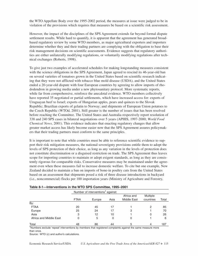
the WTO Appellate Body over the 1995-2002 period, the measures at issue were judged to be inviolation of the provisions which requires that measures be based on a scientific risk assessment.

However, the impact of the disciplines of the SPS Agreement extends far beyond formal disputesettlement results. While hard to quantify, it is apparent that the agreement has generated broad-based regulatory review by some WTO members, as major agricultural exporters and importersdetermine whether they and their trading partners are complying with the obligation to base theirrisk management decisions on scientific assessments. Evidence suggests that regulatory authori-ties are either unilaterally modifying regulations, or voluntarily modifying regulations after tech-nical exchanges (Roberts, 1998).

To give just two examples of accelerated schedules for making longstanding measures consistentwith the science obligations in the SPS Agreement, Japan agreed to rescind its 46-year-old banon several varieties of tomatoes grown in the United States based on scientific research indicat-ing that they were not afflicted with tobacco blue mold disease (USDA), and the United Statesended a 20-year-old dispute with four European countries by agreeing to allow imports of rho-dodendron in growing media under a new phytosanitary protocol. More systematic reports,while far from comprehensive, reinforce the anecdotal evidence. WTO members collectivelyhave reported 35 negotiated or partial settlements, which have increased access for: exports ofUruguayan beef to Israel; exports of Hungarian apples, pears and quinces to the SlovakRepublic; Brazilian exports of gelatin to Norway; and shipments of European Union potatoes tothe Czech Republic (WTOd, 2001). Still greater is the number of issues that has been resolvedbefore reaching the Committee. The United States and Australia respectively report resolution of338 and 240 SPS cases in bilateral negotiations over 5 years (APHIS, 1997-2000; World FoodChemical News, 2001). This evidence indicates that enacting regulatory changes that allowgreater market access has likely become easier now that the SPS Agreement assures policymak-ers that their trading partners must conform to the same principles.

It is important to note that while countries must be able to reference scientific evidence to sup-port their risk mitigation measures, the national sovereignty provisions entitle them to adopt thelevels of SPS protection of their choice, as long as any variation in the levels of protection doesnot constitute discrimination or a disguised restriction on trade. The SPS Agreement thus leavesscope for importing countries to maintain or adopt exigent standards, as long as they are consis-tently rigorous for comparable risks. Conservative measures may be maintained under the agree-ment even when these measures fail to increase domestic welfare. To cite but one example, NewZealand decided to maintain a ban on imports of bone-in poultry cuts from the United Statesbased on an assessment that shipments posed a risk of three disease introductions in backyard(i.e., noncommercial) flocks per 100 importation years (Ministry of Agriculture and Forestry,


Table 8-1—Interventions in the WTO SPS Committee, 1995–2001

Number of interventions1 against:Africa and Multiple

FTAA Europe Asia Middle East countries TotalBy:

FTAA 20 45 17 1 2 85Europe 25 24 17 3 1 70Asia 3 12 10 1 0 26Africa and Middle East 0 5 0 0 1 6

Total 48 86 44 5 4 1871Numbers exclude ‘repeat’ interventions by members that registered complaints against the same measure more than once.Source: WTO (c) and author’s calculations.

2000). Such policies may be scientifically justifiable, but nonetheless fail cost-benefit tests ifthey ignore the benefits of imports to domestic consumers.

Provisions in the agreement, which (1) recommend that countries take into account the objectiveof minimizing negative trade effects, and (2) require that measures be no more trade restrictivethan necessary, alludes to a larger role for economics in SPS policy choice. These two provisionsclearly do not require SPS measures to be justified by the economic welfare effects on produc-ers, consumers, taxpayers, and industries which use the regulated product as an input, but atleast envision consideration of economic factors that extend beyond the potential risk-relatedcosts of imports. Greater gains from trade could be realized if FTAA countries adopted a norma-tive framework which would account for the benefits as well as the potential costs of imports,but requiring (rather than just allowing) countries to do so may be seen as an unacceptableinfringement on national sovereignty.

Regionalization. The agreement’s regionalization provision is an integral part of a science-basedapproach to regulating trade, as SPS risks often do not correspond to political boundaries.Regionalization provides countries with an opportunity to export products from areas where ani-mal or plant health risks are considered negligible, thereby benefiting consumers without jeop-ardizing the agricultural resource base in the importing country. By ensuring that partial eradica-tion or control leads to trade gains, regionalization also provides incentives for additional invest-ments in control measures, so that over time this provision is likely to be of growing importancein international agricultural markets.

The trade effects of regionalization are already evident in the Western Hemisphere. Chile’s deci-sion to allow imports of fresh melons and watermelons from all production areas in the UnitedStates except Hawaii provides one example of a regional approach to mitigating pest risks(WTOh, 2001). Developing-country exporters have also benefited from regionalization: oneprominent example is provided by the United States’ 1997 decision to replace its 83-year-oldban on imports of Mexican avocados with measures that allow imports from specified regions ofMexico to the U.S. Northeast (Roberts, 1997). This measure was subsequently amended toextend the length of the shipping season and to increase the number of States that can importMexican avocados, and U.S. authorities now are considering opening access to all 50 States.

In general, however, farmers and ranchers in developing countries will face more challenges incapitalizing on the regionalization provisions than developed country producers, because exportswill be contingent on adequate public sector investments in laboratory, inspection, monitoring,and certification infrastructure. Argentina’s recent experience with outbreaks of foot and mouth


Table 8-2—Interventions in the WTO SPS Committee, by regulatory objective, 1995-20011

Total FTAA intraregionalNumber Percent Number Percent

Food safety 57 30 3 15Protection from TSEs2 50 27 1 5Plant health 42 22 9 45Animal health 33 18 7 35Other concerns 5 3 0 0Total 187 100 20 1001Numbers exclude ‘repeat’ interventions by members that registered complaints against the same measure more thanonce.2Transmissable spongiform encephalopathies.Source: WTO (c) and author’s calculations.

disease (FMD) illustrates the importance of such investments. The United States and Canada, aswell as several other countries, lifted longstanding bans on Argentina’s exports of fresh, chilled,or frozen beef in 1997 as the country neared completion of its FMD eradication program.Exports of Argentine beef to the United States reached 45,000 metric tons in 1999, but the fol-lowing year U.S. market access for the beef was suspended when FMD was detected in animalsthat had been smuggled across the border. The United States re-opened its market to Argentinebeef in December 2000, subject to certification that the beef came from FMD-free regions(along with other requirements). However, recurring outbreaks led the United States and Canadato reinstate their bans in early 2001.

This episode underscores the fact that investments in public sector regulatory infrastructure mustbe forthcoming if there is to be a return on private sector eradication efforts. It is also evidentthat national regimes will not work in some cases: trans-border pest or disease controls may berequired where there are insufficient natural barriers or when animals (including wildlife) movefreely across borders. It is therefore likely that creating or reinforcing regional sanitary and phy-tosanitary regimes across as well as within countries will often be necessary to fully realize thegains from trade in the region. Coordination of this sort may be beyond the institutional capabil-ities of some FTAA countries.

Equivalence. The SPS Agreement requires members to accept other countries’ measures asequivalent to their own if an exporter shows that its measures achieve the importer’s desiredlevel of SPS protection. This provision recognizes that regulatory flexibility allows countries toallocate scarce resources efficiently rather than identically. The agreement also encourages mem-bers to create bilateral and multilateral agreements to foster equivalence.

Equivalence determinations usually involve process standards, since countries can easily com-pare product standards, which stipulate observable and/or testable attributes of end products. Anenormous number—and arguably a growing proportion—of SPS measures are process stan-dards. One of the principal lessons to emerge from 2 decades of environmental regulation is thatprocess standards are generally an inefficient means of achieving regulatory goals. However,food technologists argue that the unique nature of food hazards—which include pathogens (suchas Salmonella) that can regenerate and cross-contaminate at several points in the productionchain—requires regulating production processes to avoid repeated, expensive tests of conformitywith product standards (MacDonald and Crutchfield, 1996). Some analysts have challenged thisconclusion (Antle, 1996), but process standards continue to emerge as components of risk man-agement programs, notably in Hazard Analysis and Critical Control Point (HACCP) programs,which an expanding number of countries mandate for a growing number of food products. Theequivalence obligation therefore theoretically has the potential to yield significant benefits ininternational markets for products such as cheeses, meats, fresh produce, and seafood for whichprocess standards are key policy instruments for managing microbial risks.

While the SPS Committee has urged members to submit information on their bilateral equiva-lence agreements and determinations, few have done so (WTOi, 2001). Consequently, there is nosystematic accounting of achievements to date. However, experts indicate that such arrange-ments are still rare (Gascoine, 1999).6 Numerous regulatory differences remain in contention


6 Possibly the most prominent equivalence accord has been a veterinary agreement signed by the U.S. and the EU inJuly 1999, after 6 years of occasionally high-profile negotiations over matters seemingly as minor as the colors ofwall paint in food-processing facilities. The veterinary agreement reduces—but does not eliminate—inspection ofsome $1 billion in EU exports of dairy products, fish, and meat to the United States, and $1 billion in U.S. exports offish, hides, and pet food to EU countries.

even between countries generally recognized as having rigorous regulatory standards that arerigorously enforced. One example is the 1997 EU ban on U.S. poultry exports: European author-ities do not consider the chlorine decontamination used in U.S. poultry processing plants equiva-lent to lactic acid decontamination.

Developing countries therefore have questioned whether the equivalence obligation will actuallyprovide many export opportunities for them, given the difficulties that developed countries havehad in exercising their rights under this provision (WTOj, 1998). A number of equivalencearrangements between developing and developed countries do exist, especially for seafood prod-ucts. However, developing countries—echoing the claims of developed countries—have arguedthat developed countries often require “compliance” rather than equivalence of measures. Evendeveloping countries that have had substantial success as agricultural exporters, such as Brazil,Mexico, and Thailand have gone on record to note the difficulties in gaining recognition ofequivalence (WTOk, 1999, and WTOl, 2001). Globally, the limited access to developed countrymarkets for poultry meat illustrates the both the potential and challenge of equivalence. Of the144 countries that are WTO members, only 15 are currently eligible to export fresh, chilled, orfrozen poultry meat to the EU, 4 may export to the U.S.,7 1 may ship to Canada, and none areallowed to export to Australia.

The United States, with the most lucrative market for developing-country exporters in theWestern Hemisphere, has stated that its experience indicates the potential for equivalence maybe limited because the actual trade benefits of an equivalence determination or agreement maynot justify the administrative burden (WTOm, 2000). The United States has also cautioned thatequivalence does not imply mutual recognition: under the equivalence provisions of the SPSAgreement, market access is contingent on a scientific determination that an exporter’s alterna-tive measure achieves the level of SPS protection required by the importer, not on reciprocity.

Multilateral harmonization. The SPS Agreement urges the widest possible harmonization ofcountries’ SPS measures based on internationally recognized standards, and identifies threeorganizations to promote this objective: the Codex Alimentarius Commission (Codex) for foodsafety measures, the International Plant Protection Convention (IPPC) for plant health measures,and the International Office of Epizootics (OIE) for animal health measures.

The agreement’s endorsement of harmonization stems from repeated complaints by exportersthat complying with divergent SPS measures substantially increases the transactions costs oftrade. The net benefits of harmonization for exporters will be positive if the resulting revenuesexceed the costs of complying with the international standard. These benefits are usually consid-ered large compared to those of regionalization or equivalence, as the former usually permitsgreater economies of scale in both production and certification. Consumers may also benefitfrom harmonization if eliminating regulatory heterogeneity among countries lowers prices andexpands product choice.

The limits to multilateral harmonization as sound policy prescription is limited by the factorsnoted earlier for regional harmonization. However, the impact of multilateral harmonization ontrade appears to have been constrained as much by the lack of international standards as by nor-mative considerations. The majority of 1995-99 notifications from WTO members stated that nointernational standard existed for the notified measure (fig. 8-1). The character of internationalstandards as a public good leads to an expectation of under-investment in their creation. Thisunderinvestment leads not only to too few international standards, but also to too many outmod-


7 In addition to the four countries that are permitted to export fresh, frozen and chilled poultry to the United States(Canada, Great Britain, France, and Israel), some plants in northern Mexico may also re-export U.S.-origin poultrymeat to the United States after minimal processing.

ed standards, which may account, in part, for the low adoption rate for those standards that doexist. Partial or full acceptance of international standards as a percentage of total measures noti-fied by income category was highest for the lower-middle income countries (38 percent) fol-lowed by high-income (22 percent), lower income (20 percent) and upper-middle income coun-tries (17 percent) (Roberts, Orden, and Josling, 1999).

The nature of international standards is also important in assessing their impact on trade. Overthe past decade, the three standards organizations have allocated most of their resources to thedevelopment of metastandards, which identify common approaches to risk identification, assess-ment, and management rather than international standards per se. In fact, the IPPC has not pro-duced any commodity-specific standards, although some are under development. Exporters’anticipated gains from international metastandards may be smaller than from international stan-dards: for example, even if an importing country has used the IPPC standard to determine thepest status of an exporting country, its measures may nonetheless vary from those of otherimporters. These metastandards have contributed to the trading system by setting out scientificapproaches to regulation, not by promulgating product standards that will be identical acrossadopting countries.

The WTO SPS Agreement and the FTAA Countries

Developed-country exporters, including the United States and Canada, are the strongest propo-nents of the current balance of rights and obligations in the WTO SPS Agreement. It is clearwhy. These countries have been able to successfully challenge measures that have no scientificbasis while maintaining their own stringent health and environmental standards that reduce veri-fiable risks to negligible levels. All four cases to advance to the WTO Appellate Body between1995 and 2002 have been won by the developed-country complainants: the United States andCanada in EC Hormones, Canada in Australia Salmon, the United States in Japan VarietalTesting, and the United States in Japan Apples (table 8-3). Developed-country exporters havealso been successful in using dispute settlement procedures to achieve their objectives beforetheir complaints reach a WTO panel. For example, Korea agreed to modify its shelf-life meas-ures in response to separate complaints from the United States (primarily for processed meats)and Canada (bottled water) as the result of formal consultations. At the same time, new initia-tives in developed countries to improve food safety, such as the U.S. Food Quality andProtection Act (FQPA), have not been challenged in the WTO even though these new policieshave resulted in lower imports from some countries.

Although many developing exporters in the region, including Chile, Argentina, and Brazil, havealso been able to capitalize on the institutional innovations established by the SPS Agreement,their intermittent success has sometimes been overshadowed by exogenous regulatory trends thatnot only frustrate attempts to expand exports, but also have reduced trade in some instances. Theincreasing demand for food safety in developed countries is the most prominent trend; another isincreased reliance on process standards that place more responsibility on the regulatory infra-structure of the exporting country than on border inspection in the importing country. A regula-tion that reflects both of these trends, the U.S. HACCP requirements for meat and poultry,resulted in a loss of market access for five developing countries (FSIS, 1999).8 Adoption of new


8 Four countries (the Dominican Republic, Guatemala, Honduras, and Slovenia) were “delisted,” which means thatthey voluntarily delisted all establishments certified for the U.S. market while developing a HACCP program. TheU.S. will not accept product from these countries until full documentation is received and evaluated to determinewhether the foreign HACCP program meets domestic requirements. Paraguay’s eligibility to export to the UnitedStates was suspended as it did not implement HACCP requirements or equivalent measures.


Table 8-3—Complaints related to SPS measures that have advanced to formal WTO dispute settlement,1995-2002

Complainant(s)Case Number(s) Issue (Co-complainants) Status

DS 3/41 Korea—produce inspection United States Settled

DS 5 Korea—shelf-life requirements United States Settled

DS 18/21 Australia—ban on salmon Canada Panel and Appellate Bodyimports (EC, India, Norway, US) ruled against Australia. Australia

notified its new measures to the WTO.

DS 20 Korea—bottled water Canada Settled

DS 26/49 EC—ban on use of United States and Canada Panel and Appellate Body ruledhormones (Australia, New Zealand, against EC. Retaliation was

Norway) authorized by the WTO when theEC failed to change its measures.

DS 76 Japan—varietal testing United States (Brazil, Panel and Appellate Body ruledrequirements EC, Hungary) against Japan. Japan has notified

its new measures to the WTO.

DS 96/1 India—quantitative EC Settledrestrictions in imports of agricultural, textile, and industrial products

DS 100 US—poultry requirements EC Pending

DS 133 Slovakia—dairy product Switzerland Pendingimports and transit of cattle (BSE restrictions)

DS 134 EU– restrictions on rice India Pending

DS 137 EU—measures on pine wood Canada Pendingnematodes in conifer wood

DS 144 US—state restrictions on Canada PendingCanadian trucks

DS 203 Mexico—measures affecting United States Pendingtrade in live swine

DS 205 Egypt—import prohibition on Thailand Pendingcanned tuna with GM soyoil

DS 237 Turkey—restrictions on Ecuador Panel suspendedfresh fruit

DS 245 Japan—apples United States Panel and Appellate Bodyruled against Japan.

DS 265 Turkey—import ban on Hungary Pendingpet food

DS 270 Australia—importation of Philippines Under review by panelfruits and vegetables

DS 271 Australia—importation of Philippines Consultationsfresh pineapple

1Some ‘pending’ cases appear to be settled, but settlement has not yet been officially notified to the WTO.Source: WTO.

HACCP measures by other developed countries has similarly led to the suspension of develop-ing country exports, particularly seafood (Unnevehr and Hirschhorn, 2000). These countriestherefore fear that without more progress on implementing the provisions of the agreement thatoffer constructive solutions to these challenges, such as regionalization, equivalence and harmo-nization, their participation in international trade will be further marginalized (WTOj, 1998).

The primary focus of developing importers, on the other hand, is on fulfilling their obligationsrather than exercising their rights under the SPS Agreement. They claim that the new obligations(related to requirements for risk assessments, for example) have diverted scarce resources frominvestments needed to capitalize on the trade opportunities created by other Uruguay Roundagreements. This group of importers, including some Central American countries and Caribbeanislands in the FTAA region, advocate various forms of increased technical assistance to addresstheir concerns (WTOn 2001; WTOo, 1999).

The varying objectives of these three groups will determine the nexus of interests for a FTAASPS agreement. The challenge before the SPS negotiators will be to find common groundamong those who favor the status quo (developed-country exporters), strengthened commitmentsto aid market access (developing-country exporters), or increased assistance to live up to currentobligations (developing-country importers). The absence of any developed-country net importers(such as Switzerland or Japan) in the Western Hemisphere should simplify the task of reachingconsensus on a regional SPS pact. Many developed importers in the WTO have proposed incor-poration of the precautionary principle in the current rules to allow more latitude for addressingconsumer concerns in SPS regulation, a suggestion that has been strongly opposed by bothdeveloped and developing exporters in the Western Hemisphere (WTOp, 2001).


Figure 8-1 Notification of adoption of international standards, by income class, 1995-99

0

100

200

300

400

500

600

700

800

Upper UpperMiddle

LowerMiddle

Lower

no. o

f not

ifica

tions

No Yes Not known Reported standard does not exist

Source: Author's calculations from WTO data.

Options for an FTAA SPS Agreement

A regional accord to discipline the use of SPS measures will differ in important respects fromthe preferential trading arrangements made for tariff and other nontariff barriers within theregion. Rules cannot be tailored for specific products of interest to regional trading partners, norestablish preferential schedules for regional exporters to comply with SPS measures. As in amultilateral agreement, a regional agreement consists of a set of rules, applicable to all FTAAcountries, that is aimed at reducing the trade distorting aspects of all SPS measures.

If new rules or principles are to be negotiated, it should be recognized that the starting point forthe FTAA negotiators will be the WTO SPS Agreement. All FTAA countries, as WTO members,are bound by the provisions in this agreement. The decentralized policing rules of the WTO SPSAgreement therefore establishes a “floor” for any regional rules. Hypothetically, even if FTAAexporters were to agree to relax the equivalence obligation for Western Hemisphere importers,the importers still would be required to recognize the equivalent measures of non-FTAAexporters. Membership in the WTO therefore limits the options of FTAA countries to eitherexisting WTO rules or to “WTO plus” rules that augment trade.

No FTAA country has yet proposed a new addition to the current WTO principles of transparen-cy, science-based risk regulation, national sovereignty, regionalization, equivalence, and multilat-eral harmonization. Rather, FTAA proposals have ranged from leaving the existing WTO rulesintact to making existing rules far more prescriptive (FTAA, 2001). This suggests that differingviews on the success or shortcomings of the WTO SPS Agreement does not involve differencesover fundamental principles, but rather implementation of the current obligations. Althoughmodifying basic treaty rules is favored by those countries who would like to improve implemen-tation of the current obligations, this option has a number of shortcomings. First, making treatyrules more prescriptive is at best a blunt tool for engineering more energetic fulfillment of obli-gations to achieve region-specific goals or outcomes. Secondly, this option also risks codifyingdetailed procedures that may be increasingly inappropriate over time. Finally, altering the basicprinciples of the WTO rules in a regional accord may eventually jeopardize coherence in riskmanagement policy as the multilateral rules evolve over time.

One remedy that can be targeted regionally, and may be especially suitable for a coalition ofdeveloped and developing countries (unlike more homogenous regions) is technical assistance.Seven years of experience with the provisions of the WTO SPS Agreement suggest the followingoptions for technical assistance to expand regional trade:

helping the region’s developing countries to eradicate or mitigate pests and diseases inspecific regions could yield substantial payoffs, because the complaints raised in the SPSCommittee identified animal and plant health measures as the more significant impedi-ments to trade in the hemisphere. Such assistance could be, in effect, extra-territorialinvestments in biosecurity for importing countries, resulting in increased foreign ship-ments that benefit domestic consumers without increasing SPS risks that could harm

domestic production;9

targeting technical assistance to the strengthening of public sector testing and certifica-tion services in the developing countries to speed equivalence determinations or compli-ance audits by developed country food safety regulators. Technical assistance could also


9 Some intergovernmental efforts to eradicate animal and plant pests, including Mediterranean fruit flies, screw-worm, and FMD are already under way in the region.

be used by developing countries to establish a separate “enclave” food system that meetshigher regional standards, while maintaining standards that are more suitable for thedomestic market given national preferences, technologies, and endowments;

using technical assistance to promote the participation of regional developing countriesin activities of the international standards organizations. It is important for new partici-pants to recognize that more widespread adoption of international standards may notalways increase trade—trading partners that adopt international HACCP standards, forexample, may still have different requirements for gaining access to domestic markets, asseen in the poultry meat sector. Nonetheless, the standards organizations are importantinstitutions for development of science-based regulation, and greater participation bydeveloping countries may contribute to the more effective functioning of internationalmarkets by increasing the predictability of regulation in these countries; and,

technical assistance to help the least developed countries in the region come into compli-ance with their obligations as importers. However, nearly every FTAA country has ful-filled the SPS transparency requirements, the most basic obligation under the WTO SPSAgreement, and the costs and benefits of investment in national risk assessment capabili-ties for least developed countries needs to be weighed against the costs and benefits ofalternative strategies, including adoption of international standards.

Technical assistance is already widely recognized as an effective mechanism for addressing SPSbarriers to trade. The WTO SPS Agreement includes an article on technical assistance that states“Members agree to facilitate the provision of technical assistance to other members, especiallydeveloping-country members ...”. If FTAA countries choose increased technical assistance as ameans of expanding regional trade, they will still have to determine how to best strengthen thecurrent WTO commitment in a regional trade pact. Institutional arrangements will also be animportant issue for negotiators. Options include establishment of new regional committees, oruse of WTO mechanisms (including existing subcommittees of the Codex Commission, theOffice of International Epizootics, and the International Plant Protection Convention) to accom-plish FTAA goals. Regardless of the outcome, FTAA policymakers will need guidance on estab-lishing priorities for SPS initiatives in the region. Economic research that could aid in the identi-fication of priority projects currently lags far behind analysis of other trade barriers. Additionalinvestments in multidisciplinary research on SPS measures therefore will be necessary if theobjective of increasing regional welfare through trade is to be realized.

References

Animal and Plant Health Inspection Service (APHIS). “SPS Accomplishment Reports,”Washington D.C., various issues, 1997–2000, Washington, D.C.

Antle, John (1996). “Efficient Food Safety Regulation in the Food Manufacturing Sector,”American Journal of Agricultural Economics, 78 (5): 1242 - 1247.

Food Safety and Inspection Service (1999). “Equivalence Evaluation of Pathogen Reduction andHACCP Requirements,” December 14, on file with author.

Gascoine, Digby (1999). “Harmonisation, Mutual Recognition and Equivalence: How and Whatis Attainable,” WHO/FAO Conference on International Food Trade Beyond 2000,” Melbourne,Australia, October.


General Agreement on Tariffs and Trade (GATT). International Trade, 1990-91, Volume 1,Geneva, Switzerland.

Free Trade Area of the Americas (2001). Draft Agreement: Chapter 1 (Agriculture), Section Five(Sanitary and Phytosanitary Measures), FTAA.TNC/w/133/Rev.1, July 3 on FTAA website athttp://www.ftaa-alca.org.

MacDonald, James and Stephen Crutchfield (1996). “Modeling the Costs of Food SafetyRegulation,” American Journal of Agricultural Economics, 78 (5): 1285-1290.

Ministry of Agriculture and Forestry, 2000. Import risk analysis: chicken meat and chicken meatproducts, Biosecurity Authority, Wellington, NZ, April 7 (on file with author).

Roberts, Donna (1997). “USDA to Lift Import Ban on Mexican Avocados.” AgriculturalOutlook, July: 17-21.

Roberts, Donna (1998). “Preliminary Assessment of the Effects of the WTO Agreement onSanitary and Phytosanitary Trade Regulations,” Journal of International Economic Law, 1 (3):377 – 405.

Roberts, Donna. L. Unnevehr, J. Caswell, I. Sheldon, J. Wilson, T. Otsuki, D. Orden. (2001).Agriculture in the WTO: The Role of Product Attributes in the Agricultural Negotiations.Presented at the International Agricultural Trade Research Consortium Annual MembershipMeeting in Washington, DC. May 18-20, 2001. Commissioned paper No. 17.

Roberts, Donna, David Orden, and Timothy Josling (1999). “WTO Disciplines on Sanitary andPhytosanitary Barriers to Agricultural Trade: Progress, Prospects, and Implications forDeveloping Countries,” invited paper, Conference on Agricultural and the New Trade Agendafrom a Development Perspective, World Bank, Geneva, October.

Sykes, Alan (1999). “The (Limited) Role of Regulatory Harmonization in International Goodsand Services Markets,” Journal of International Economic Law, 2(1): 49–71.

Sykes, Alan O. (1995). Product Standards for Internationally Integrated Goods Markets, TheBrookings Institution, Washington, DC.

Unnevehr, Laurian, and Nancy Hirschhorn ( 2000). “Food Safety Issues in the DevelopingWorld,” World Bank Technical Paper No. 469, World Bank, Wash., D.C.

World Food Chemical News, 2001. “Quarantine laws cited as way to gain market access,”September 10, p. 11.

World Trade Organization (WTOa) 1999. “Review of the Agreement on the Application of theSanitary and Phytosanitary Agreement,” G/SPS/12, March 11, on WTO website athttp://www.wto.org.

WTO (b) 2001. “Implementation-Related Issues and Concerns–Decision of 14 November,”WT/MIN(01)/17, November 20, 2001 on WTO website at http://www.wto.org.



WTO (c). “Summaries of the Meetings of the Committee on Sanitary and PhytosanitaryMeasures,” Sanitary and Phytosanitary Committee, G/SPS/R series, 1995–2001, on WTO web-site at http://www.wto.org.

WTO (d) 2001. “Specific Trade Concerns,” Note by the Secretariat, Sanitary and PhytosanitaryCommittee, G/SPS/GEN/204/Rev.1, March 5, 2001 on WTO website at http://www.wto.org.

WTO (e) 1999 and 2002. “Recommended Notification Procedures,” Sanitary and PhytosanitaryCommittee, G/SPS/7/Rev.1, November 26, and G/SPS/R/Rev. 2, April 2, on WTO website athttp://www.wto.org.

WTO (f) 2001. “Agreement on the Application of Sanitary and Phytosanitary Measures:Proposal by Brazil,” G/SPS/W/108, June 22, on WTO website at http://www.wto.org.

WTO (g). 2001. “Enhancing Transparency: Proposed Changes to The RecommendedNotification Proedures,” Submission by New Zealand, G/SPS/W/112, October 15, on WTO web-site at http://www.wto.org.

WTO (h) 2001. “Notification,” Sanitary and Phytosanitary Committee, G/SPS/N/CHL/56,November 11, on WTO website at http://www.wto.org.

WTO (i) 2001. “Equivalence: Note by the Secretariat,” G/SPS/W/111, July 4, 2001, on WTOwebsite at http://www.wto.org.

WTO (j). 1998. “The WTO SPS Agreement and Developing Countries,” Committee on Sanitaryand Phytosanitary Measures, G/SPS/W/93, November 5, on WTO website athttp://www.wto.org.

WTO (k) 1999. “Summary of the Meeting Held on 7–8 July, 1999”, Sanitary and PhytosanitaryCommittee, G/SPS/R/15, October 29, on WTO website at http://www.wto.org.

WTO (l) 2001. “Experience with Recognition of Equivalence: Statement by Thailand,”G/SPS/GEN/242, April 6, on WTO website at http://www.wto.org.

WTO (m) 2000. “Equivalence: Submission from the United States,” G/SPS/GEN/212,November 7, on WTO website at http://www.wto.org.

WTO (n). 2000. “Proposal by Small Island Developing States”,G/AG/NG/W/97, December 29,on WTO website at http://www.wto.org.

WTO (o) 1999. “Development and Adaptation of Sanitary and Phytosanitary Systems inDeveloping Countries for the Purpose of Complying with Commitments under the Agreement onthe Application of Sanitary and Phytosanitary Measures: Statement by Guatemala, December 17,on WTO website at http://www.wto.org.

WTO (p) 2000. “Note on Non-Trade Concerns,” Submission to the Third Special Session of theWTO Committee on Agriculture, G/AG/NG/W/36, September 22, on WTO website athttp://www.wto.org.

Appendix 1-1

A CGE Model

The computable general equilibrium (CGE) model used in this chapter is composed of 16 coun-tries or regions linked by trade. There are nine primary agriculture sectors and six processedfood sectors; the other sectors in the economy are broadly defined as natural resources, manu-facturing, and services.1 The model data are from the Global Trade Analysis Project (GTAP)version 5, August 2002 update. The model base year is 1997, with results adjusted to 2002 dol-lars using the U.S. gross domestic product (GDP) deflator (U.S. OMB, 2003).

The model follows the standard neoclassical specification of trade-focused CGE models. Eachsector produces a composite commodity that can be transformed according to a constant elastici-ty of transformation (CET) function into a commodity sold on the domestic market or into anexport. Output is produced according to a constant elasticity of substitution (CES) productionfunction in primary factors, and fixed input-output coefficients for intermediate inputs. Themodel simulates a market economy, with prices and quantities assumed to adjust to clear mar-kets. All transactions in the circular flow of income are captured. Each country model traces theflow of income (starting with factor payments) from producers to household, government, andinvestors, and finally back to demand for goods in product markets.

Consumption, intermediate demand, government, and investment are the four components ofdomestic demand. Consumer demand is based on Cobb-Douglas utility functions, generatingfixed expenditure shares. Households pay income taxes to the government and save a fixed pro-portion of their income. Intermediate demand is given by fixed input-output coefficients. Realgovernment demand and real investment are fixed exogenously. Import demand is described byalmost-ideal demand system (AIDS) import demand functions.

The model includes three primary factors and associated factor markets: labor, capital, andagricultural land. Land is disaggregated into two types-cereals and oilseeds, and all other land.Full employment for all categories is assumed, and aggregate factor supplies are fixed. In theexperiments reported here, we assume that all factors are fully mobile. However, land marketsare segmented. Land used in cereals and oilseeds cannot be substituted for land used to pro-duce other crops.

There are three key macro balances in each country model: the government deficit, aggregateinvestment and savings, and the balance of trade. Government savings are the differencebetween revenue and spending, with real spending fixed exogenously, and revenue depending ona variety of tax instruments. The government deficit is therefore determined endogenously. Realinvestment is set exogenously and aggregate private savings are determined residually to achievethe nominal savings-investment balance. The balance of trade for each country (and hence for-eign savings) is set exogenously and valued in world prices. Each model solves for the relativedomestic prices and factor returns that clear the factor and product markets, and for an equilibri-um real exchange rate which brings aggregate export supply and import demand into balance,given the exogenous aggregate trade balance of each country.

The model incorporates budgetary expenditure for 2001 domestic farm programs in theEuropean Union, Japan, Canada and Mexico from the OECD Producer Support Estimate data-


1 We use the standard global CGE model described in Lewis, Robinson, and Thierfelder (2003).

base for 2001 (OECD, 2002). Data for U.S. farm programs are the annual average of July2002 projected expenditures under the Farm Security and Rural Investment Act. The modelincorporates endogenous farm programs, where applicable, following Burfisher, et al. (2002).In the U.S., loan deficiency payments support floor prices for grains and oilseeds, with pay-ments to farmers increasing when market prices decline below the loan rate. In the EU andCanada, export subsidies are used to clear excess domestic supplies resulting from the EU’sfixed intervention prices for grain, oilseeds and livestock, and Canada’s price managementprogram for dairy.

Other farm payments are exogenous income transfers to households. These include direct pay-ments and countercyclical payments in the United States, Canada (National Income StabilizationAccounts or NISA payments) and Mexico (PROCAMPO, the Farmers Direct Support Program).Households spend these transfers on consumption, savings and taxes according to the aggregateaverage propensities described in national accounts data.

The model also includes fixed, per unit ad valorem subsidies to inputs and output. Since the pro-duction technology in the model uses fixed input-output coefficients for intermediate inputs, asubsidy to intermediate goods operates like an output subsidy. Subsidies on capital inputs inagriculture lower the costs of capital and attract capital out of non-agricultural sectors.

The model uses data on tariffs and tariff equivalents from various sources. MFN agricultural tar-iffs for all countries are from the Agriculture Market Access Database (AMAD). AMAD pro-vides tariffs on an ad-valorem basis, including the ad valorem equivalents of specific tariffs.Tariff rate quotas are modeled as ad valorem tariffs using the average of above and below quotatariff rates. AMAD tariffs are aggregated to the GTAP categories using import weights.

This chapter develops a preferential agricultural tariff database for U.S. GSP, ATPA andCaribbean Basin Economic Recovery Act (CBERA) programs, and for Canadian GPT andCaribbean preferences. Preferential tariff data for the U.S. and Canada are from their tariffschedules for 2000, aggregated to GTAP categories using simple averages. In MERCOSUR andChilean bilateral trade pacts, agricultural tariffs in the model are assumed to be zero, althoughMERCOSUR, the Andean Community, and other preferential agreements in the WesternHemisphere allow some exceptions to their common external tariffs and zero internal tariffs(Stout and Ugaz-Pereda, 1998). This assumption may therefore lead to an underestimate of theFTAA’s effects.

Following de Melo and Robinson (1992), the model incorporates links between the expansion ofexports and imports of capital goods between developing and developed countries and techno-logical spillovers that stimulate factor productivity growth in the developing country. Trade isassumed to have a role in stimulating productivity growth through channels that include technol-ogy differences among countries, knowledge spillovers, the transmission of ideas, and marketexpansion that leads to increasing returns to scale and/or Smithian economies of “fine special-ization” (as opposed to Ricardian differences in factor proportions). A sectoral export externalitylinks export growth in manufactures to an increase in total factor productivity (TFP) within thesector. An import externality links imports of manufactures with sectoral TFP. Finally, anincrease in aggregate exports leads to economy-wide increases in the efficiency of capital inputs.Note, however, the conditions that must be in place for productivity growth to be accelerated arelikely to include not only tariff reform, but also factors such as institutional reforms that facili-tate investment and trade (Rodrick et al., 2002).



Appendix Table 1-1 A—Change in U.S. agricultural exports due to an FTAA ($U.S. billion)

C. America & Rest S. Total Rest of Canada Mexico Caribbean Andean Argentina Brazil Chile America FTAA world World

Rice, raw 0 -2 102 12 0 0 0 0 112 -14 98Wheat 0 2 22 45 0 0 0 1 70 -11 59Other grains -8 -27 56 60 12 1 3 0 98 -7 91Horticulture -7 1 34 22 3 10 1 0 65 -30 35Oilseeds 1 -9 14 29 32 30 1 0 98 -21 77Other crops -3 0 66 32 13 21 1 0 129 -39 90Livestock -3 -2 19 4 4 3 1 0 26 -33 -7Meat -8 -1 77 25 2 4 0 2 102 -52 50Oils and fats 0 -3 64 67 1 3 2 1 135 -10 125Dairy prods. 203 -2 25 10 2 3 0 1 242 -10 232Processed foods -16 1 171 57 34 45 8 25 325 -110 215Total agric. 159 -43 649 363 104 121 18 31 1401 -336 1,065


Appendix Table 1-1 B—Change in U.S. agricultural imports due to an FTAA ($U.S. million)

C. America & Rest S. Total Rest of Canada Mexico Caribbean Andean Argentina Brazil Chile America FTAA world World

Rice, raw 0 0 0 0 0 0 0 0 0 8 8Wheat 1 0 0 0 0 0 0 0 1 0 1Other grains 34 0 0 0 1 0 3 0 38 4 43Horticulture 0 5 14 1 1 10 22 0 54 1 55Oilseeds 0 0 1 0 0 3 0 0 4 0 4Other crops 1 3 15 5 1 24 2 0 53 2 55Livestock 27 3 0 0 1 1 0 0 33 13 46Meat 9 0 1 0 0 2 0 1 13 9 22Oils and fats 3 0 0 0 0 1 0 0 4 4 9Dairy prods. 0 0 1 0 4 0 0 1 7 7 13Processed foods 10 3 279 164 47 91 75 10 679 39 718Total agric. 86 15 311 171 56 133 102 12 886 88 974


Appendix Table 1-1 C—Average agricultural tariff rates of FTAA members on imports from WesternHemisphere, by country and commodity

Central Rest. S.U.S. Canada Mexico America Andean Argentina Brazil Chile World

Rice 4.2 0.3 9.0 30.2 16.0 6.8 9.8 3.8 8.5Wheat 0.9 41.9 15.4 0.6 6.8 2.0 2.3 5.1 0.7Other grains 0.2 4.4 17.9 4.7 9.4 2.9 3.6 6.5 1.5Fruits & vegetables 3.8 1.5 13.3 15.8 14.7 9.0 9.0 8.6 10.4Oil seeds 14.4 0.0 1.5 2.9 6.3 3.7 4.4 7.8 1.2Raw sugar 0.1 0.0 5.7 1.7 0.4 0.7 1.3 2.1 0.0Other crops 17.3 2.0 7.6 8.3 8.8 7.7 6.9 8.1 7.0Livestock 0.6 11.6 7.8 10.2 8.2 4.9 5.8 8.6 5.0Meat manufacturing 3.6 41.6 40.3 16.7 16.5 9.7 10.5 8.7 11.7Oils & fats 3.6 4.5 15.7 9.5 15.3 7.3 8.6 7.6 8.9Dairy manufacturing 34.4 202.4 33.5 23.9 16.7 14.4 15.9 4.8 22.5Processed sugar 43.6 2.7 1.4 12.5 10.5 9.6 12.0 8.5 10.7Processed foods 8.2 21.0 16.1 15.2 16.5 13.9 14.9 9.1 15.2Manufacturing 3.4 4.2 8.9 9.3 11.7 11.0 11.0 8.9 10.9Average agric. tariff 10.4 25.7 14.2 11.7 11.3 7.1 8.1 6.8 7.9Ratio ag. to mfg. tariff 3.1 6.2 1.6 1.3 1.0 0.6 0.7 0.8 0.7Sources: AMAD, U.S. and Canadian 2000 harmonized tariff schedules. Tariff rates include bilateral preferential tariff rates.

Appendix 2-1

Description of Methodology

Econometric Approach. In the not too distant past, most gravity models of international tradewere estimated using ordinary least squares, and this approach continues to be applied by manyresearchers. However, the data sets that describe bilateral trade flows usually lack observationsfor those instances where trade equaled zero or was not reported. This is particularly true at thecommodity level, where the proportion of such observations can be rather high. Since this char-acterization applies to the database used in this chapter, the modified gravity models here areestimated as tobit models, as presented by Green (pp. 727-729):(1)

where y*it is latent measure of trade. The observed, dependent variable (yit) equals the log of U.S.

exports to country i in year t, as measured in U.S. dollars.

The number of missing observations in the export data increase as one moves backwards in timethrough the data set, so the sample is restricted to the 1980-1999 period to ensure that missingobservations do not drive the results. In addition, a country’s observations are included only ifthere are at least 10 nonzero observations (out of 14) during 1980-1993 and at least 5 non-zeroobservations (out of 6) during 1994-99. This evaluation is conducted on a model-by-model basis.Thus, the set of countries included in the model of total agricultural exports is substantially larg-er than the sets used in the commodity models.

Explanatory Variables. In addition to the intercept, the models in this chapter contain a num-ber of explanatory variables. The log of the importing country’s GDP accounts for variationsin U.S. exports due to the size of the importing economy. This variable, measured in U.S. dol-lars, is drawn primarily from the International Monetary Fund’s World Economic OutlookDatabase. GDP data for countries not in this database are from the Statistical Yearbook of theUnited Nations.

Although population estimates are readily available in the World Bank’s World DevelopmentIndicators CD-ROM and the United Nations’ Demographic Yearbook, the models employed heredo not include the log of the importing country’s population, a variable that appears in manyprevious gravity models. This decision is motivated by the fact that the log of population isclosely correlated to the log of GDP. According to 1995 data, the correlation coefficient betweenthe two variables is 0.70 for the 127 countries in the sample.

Trade-Agreement Variables. Of primary interest are the explanatory variables that indicate acountry’s participation in a particular trade agreement (table 2-2). Unlike most previous works,these variables are country-specific in order to address the possibility that the impact of a tradeagreement varies among its participants. This possibility is especially strong in the case ofNAFTA, which took effect on January 1, 1994, and will complete its implementation phase onJanuary 1, 2008. NAFTA includes three distinct schedules for tariff elimination: a U.S. schedulefor Mexican exports, a Canadian schedule for Mexican exports, and a Mexican schedule for U.S.and Canadian exports. Moreover, NAFTA subsumes CFTA and its tariff-elimination schedulesfor U.S.-Canada trade.


ititit xy εβ +′=* ,

0=ity if 0* ≤y ,*itit yy = if 0* >y ,

CFTA took effect on January 1, 1989, and its provisions were fully implemented on January 1,1998. Thus, the first 5 years of NAFTA (1994-98) coincide with the last 5 years of CFTA’s tar-iff-elimination schedule. To distinguish the impact of this latter phase of CFTA’s implementationfrom the agreement’s broad influence since 1989, the models include two variables that identifyexports to Canada during the CFTA/NAFTA period: CFTA-Canada (1989-1999) and NAFTA-Canada (1994-99).

For Mexico, NAFTA is the extension of a process of unilateral trade reforms that followed thecountry’s accession to the General Agreement on Tariffs and Trade (GATT) in 1986. In the late1980s and early 1990s, Mexico dramatically reduced its tariffs and opened its economy to for-eign direct investment. Import licensing was eliminated for many agricultural products, and tar-iffs were established well below the 50-percent ceiling established by Mexico’s GATT AdhesionProtocol. U.S. exports that benefited from these reforms include beef, pork, sorghum, soybeans,and other oleaginous crops (Rosenzweig Pichardo, 2000). Because Mexico is one of the mostimportant customers for U.S. agricultural products, these reforms may be viewed as a predeces-sor to NAFTA, somewhat akin to CFTA. For this reason, the models employ two variables tomeasure trade liberalization’s impact on exports to Mexico: Unilateral-Mexico (1989-1999) andNAFTA-Mexico (1994-99). The year 1989 is selected as the beginning of the period covered byUnilateral-Mexico to account for the piecemeal implementation of the reforms over a long peri-od, as well as the fact that key agricultural trade reforms were implemented after 1989.

All four variables listed above are hypothesized to have a positive impact on U.S. agriculturalexports, as these measures have provided the United States with substantially freer access to theCanadian and Mexican markets. In contrast, the process of regional integration in South Americamay have positive or negative effects on U.S. exports. Argentina, Brazil, Paraguay, and Uruguaycreated MERCOSUR through the Treaty of Asunción, which took effect on November 29, 1991.By progressively eliminating most tariff barriers within the common market, MERCOSUR pro-vides its members with preferential access to each other’s markets. Since the United States is notpart of MERCOSUR, this process may divert potential U.S. exports from the common market.

However, MERCOSUR also provides for a common external tariff ranging from zero to 20 per-cent towards non-member countries. In many instances, this tariff is substantially lower than thetariff previously applied by the individual MERCOSUR countries. Thus, its implementation mayspur additional U.S. exports to the common market. In addition, Chile and Bolivia became asso-ciate members of MERCOSUR in 1996 and 1997, respectively. This means that they share inMERCOSUR’s project of internal trade liberalization but do not apply the common external tariff.

To gauge MERCOSUR’s impact on U.S. exports, four variables identify exports to particularMERCOSUR countries following the common market’s creation: Argentina/1991-99,Brazil/1991-99, Paraguay/1991-99 and Uruguay/1991-99. Four more variables(Argentina/1994-99, Brazil/1994-99, Paraguay/1994-99, and Uruguay/1994-99) indicateexports to these countries during 1994-99. This latter group of variables is intended to capturethe additional effect associated with the progressive reduction of tariffs within MERCOSUR, aswell as NAFTA’s possible influence on U.S. exports to MERCOSUR. Finally, two variables(Bolivia/1997-99 and Chile/1996-99) identify exports to Bolivia and Chile following theirbecoming associate members of MERCOSUR.

The coefficient for each trade-agreement variable measures the shift in the intercept associatedwith the observations denoted by that variable. As an example, consider the results for CFTA-Canada in the model of total agricultural exports (table 2-3). The coefficient for this variable


(0.3758) equals the difference between the expected value of the latent trade variable y*it when

CFTA-Canada equals zero and the expected value of y*it when CFTA-Canada equals one.

Expected Value of the Dependent Variable. Following Green (p. 728), the expected value ofthe dependent variable (the log of exports to country i in year t) equals

By subtracting the model’s coefficient for Unilateral-Mexico (0.4987) from and then sub-

stituting this difference for in equation (2), one may calculate the expected value of U.S.agricultural exports to Mexico during 1989-1993 when Unilateral-Mexico is held equal to zero.Similarly, for corresponding exports during 1994-99, one may calculate the expected value whenUnilateral-Mexico and NAFTA-Mexico are held to zero by also subtracting the coefficient for

NAFTA-Mexico (0.3892) from when re-calculating the equation. This technique providesthe basis for a simple simulation of what the value of U.S. agricultural exports to Mexico wouldhave been in the absence of NAFTA and Mexico’s unilateral reforms.

itxβ ′

itxβ ′itxβ ′


(2) ( )ititit

itit xx

xyE σλβσ

β+′⎟

⎠⎞⎜

⎝⎛ ′

Φ=]|[ ,

where( )( )σβ

σβφλ

/'/'

it

itit x

xΦ

=

and σ is the model’s scale parameter.

Appendix 2-2

The International Bilateral Agricultural Trade Database

The export data for the models are drawn from the International Bilateral Agricultural Trade(IBAT) database. This unique statistical resource, developed by Mark J. Gehlhar of ERS, reflectsan innovative effort to choose among the competing trade statistics reported to the UnitedNations. Given the trade statistics reported by two countries, the IBAT database includes the fig-ures from the country with the larger share of reported trade that matches the reported trade ofits trading partners. This evaluation is conducted on an annual basis at the 4- and 5-digit level ofthe Standard Industrial Trade Classification (SITC). Countries in the sample are listed in appen-dix table 2-1.

A relatively simple example from Argentina-Brazil trade helps to illustrate this process. Asreported to the United Nations, the official statistics of Argentina and Brazil contain incompati-ble measures of Argentine wheat exports to Brazil in 1995. This trade equaled $662 millionaccording to Argentina, but just $4 million according to Brazil. Fortunately, the entire body ofstatistics reported by Argentina, Brazil, and their trade partners provides insight into the generalreliability of the two countries’ trade reports. With this information, one may calculate a“Reliability Index” for Argentina’s wheat export data and for Brazil’s wheat import data for1995. This index is defined as the proportion of a country’s reported trade that matches the sta-tistics of its partners. Then, the statistic with the higher Reliability Index is included in the IBATdatabase. With the assistance of a computer, this decision rule can be elegantly applied to all thebilateral trade data reported to the United Nations—commodity by commodity, year by year, andcountry by country.

Consider first the wheat export data of Argentina (appendix table 2-2). A match is defined ashaving occurred when Argentina’s reported exports to country i equal the imports fromArgentina reported by country i, plus or minus 20 percent. Eight of Argentina’s reported bilateralexport flows qualify as matches, for a total of $128 million. This value forms the numerator ofthe Reliability Index. The denominator equals the sum of Argentina’s reported export flowswhere both Argentina and the importing country report some non-zero level of trade ($128 mil-lion + $797 million = $925 million), minus the value associated with the largest proportionatediscrepancy ($662 million). In this instance, Brazil is the country with the largest discrepancy.Thus, the denominator equals $263 million ($925 million - $662 million), and the ReliabilityIndex for Argentina’ wheat export statistics for 1995 equals 0.49.

Next, consider the wheat import data of Brazil. For 1995, Brazil reported wheat imports fromonly two sources: Argentina ($4 million) and Paraguay ($1 million). A match occurs whenBrazil’s reported imports from country i equal the exports to Brazil reported by country i, plusor minus 20 percent. Neither figure qualifies as a match, so the Reliability Index for Brazil’swheat import statistics for 1995 is zero. Since 0.49 is greater than zero, the IBAT databaserecords Argentine wheat exports to Brazil in 1995 as $662 million, not $4 million.

With respect to U.S. trade, the IBAT database primarily uses information provided by the UnitedStates, which has the higher Reliability Index in most face-to-face comparisons. But U.S. data arenot used on every occasion. Appendix table 2-3 lists the proportion of observations in the IBATdatabase that were reported by the United States for the 32 commodity categories featured in thecommodity models. Among these commodities, grapes have the highest proportion of U.S. obser-vations (0.767) and sunflower seed oil has the lowest (0.519). The median proportion is 0.6485,



Appendix Table 2-1—Countries appearing in sample

Algeria Guinea PeruAngola Guyana PhilippinesArgentina Honduras PolandAustralia Hong Kong PortugalAustria Hungary QatarBahamas Iceland RomaniaBahrain India SamoaBangladesh Indonesia Saudi ArabiaBarbados Ireland SenegalBelgium and Luxemburg Israel SeychellesBelize Italy Sierra LeoneBenin Ivory Coast SingaporeBermuda Jamaica Solomon IslandsBolivia Japan SomaliaBrazil Jordan South Africa Customs Union (5)Brunei Darsm Kenya Soviet Union, former (6)Bulgaria Korea SpainBurkina Faso Kuwait Sri LankaCameroon Lebanon St. Kitts, Nevis, and AnguillaCanada Liberia SudanCentral African Republic Macau SurinameChile Madagascar SwedenChina, mainland Malaysia SwitzerlandColombia Mali SyriaCongo Malta Taiwan (7)Costa Rica Mauritania TanzaniaCyprus Mauritius ThailandDenmark Mexico TogoDominican Republic Morocco Trinidad and TobagoEcuador Mozambique TunisiaEgypt Myanmar TurkeyEl Salvador Nepal UgandaEquatorial Guinea Netherlands United Arab EmiratesEthiopia, former (1) Netherlands Antiles (3) United KingdomFiji New Caledonia (4) United StatesFinland New Zealand UruguayFrance (2) Niger VenezuelaGabon Nigeria YemenGambia Norway Yugoslavia, former (8)Germany, united Oman ZaireGhana Pakistan ZambiaGreece Papua New Guinea ZimbabweGuatemala Paraguay(1) Djibouti, Ethiopia, and Eritrea(2) Also includes French Guiana, Guadeloupe, Martinique, and Reunion(3) Curacao, Aruba, and Turks and Caicos Islands(4) Also includes Wallis and Futana Islands(5) Botswana, Lesotho, Namibia, South Africa, and Swaziland(6) Armenia, Azerbaijan, Belarus, Estonia, Georgia, Kazakshtan, Kyrgyzstan, Latvia, Lithuania, Moldova, RussianFederation, Tajikistan, Turkmenistan, Ukraine, and Uzbekistan(7) Asia, not elsewhere specified(8) Bosnia-Herzogovia, Croatia, Slovenia, Macedonia (Skopje), and Yugoslavia


Appendix Table 2-2—Competing reports of Argentine wheat exports, 1995

Reported Exports (x) Reported Imports (m) m / xImporting Country $U.S. thousands

Exporter reports no trade

Egypt 0 3,687 n.a.

Greece 0 3,231 n.a.

Italy 0 1 n.a.

Switzerland 0 169 n.a.

Importer reports no tradeAngola 943 0 0.00

Bangladesh 4,534 0 0.00

Iran 25,754 0 0.00

Kenya 35,926 0 0.00

Mozambique 6,603 0 0.00

Netherlands 20 0 0.00

Tanzania 2,556 0 0.00

Yemen Rep. 4,016 0 0.00

Total, non-reporting importers (A) 80,352

Both countries report trade, large discrepanciesBolivia 879 2,129 2.42

Brazil 661,878 4,457 0.01

Chile 21,289 28,232 1.33

Colombia 10,110 14,736 1.46

Indonesia 60,549 94,750 1.56

Jordan 26,971 14,218 0.53

Paraguay 11,417 5,934 0.52

Reunion 108 142 1.32

Spain 6 8 1.40

Zimbabwe 3,533 9,183 2.60

Total, large discrepancies (B) 796,740

Both countries report trade, small discrepanciesChina 34,176 39,705 1.16

Germany 6 7 1.09

Malaysia 657 791 1.20

Peru 71,243 85,564 1.20

South Africa 6,399 5,218 0.82

Turkey 7,250 8,482 1.17

Uruguay 122 139 1.14

Venezuela 8,429 7,164 0.85

Total, small discrepancies (C) 128,282

Total exports (D = A + B + C) 1,005,374

Total, non-reporting importers (A) 80,352

Observation with largest proportionate 661,878 (Brazil)discrepancy (B*)

Qualified reported exports 263,144

(E = D - A - B*)

Total, small discrepancies (C) 128,282

Reliability Index (RI = C / E) 48.8Source: Economic Research Service.

which is the average of the proportions for corn (0.648) and cotton (0.649). The possibility that asmany half of U.S. trade reports for certain commodities could be inferior to the reports submittedby U.S. trade partners provides strong justification of the IBAT database’s selective approach.


Appendix Table 2-3—Proportion of observations in IBAT database that were reported bythe United States, U.S. exports, 1980-99, by commodity (number of observations reportedby United States divided by total observations)

Beer 0.586 Pork (fresh or frozen) 0.760

Cheese 0.519 Poultry (fresh or frozen) 0.583

Distilled alcoholic beverages 0.592 Milk and cream 0.548

Cotton 0.649 Edible nuts 0.609

Flowers and foliage (cut) 0.671 Plants and bulbs (live) 0.715

Fruit or vegetable juice 0.731 Prepared breakfast food 0.666

Apples (fresh) 0.621 Soda and bottled water 0.706

Grapes (fresh) 0.767 Soybean oil 0.597

Corn 0.648 Soybeans 0.596

Rice 0.567 Sunflower seed oil 0.514

Wheat 0.549 Tobacco (unmanufactured) 0.753

Peanuts 0.723 Tobacco products 0.600

Leather 0.545 Tomatoes 0.708

Live poultry 0.588 Legumes 0.647

Macaroni 0.746 Wine 0.714

Beef (fresh or frozen) 0.738 Yarn and thread 0.603Source: Economic Research Service.

Appendix 3-1

It is no easy task to even approximately measure the protective effect of a country’s tariff sched-ule by collapsing it into a single measure such as a mean. Undeterred by this difficulty, econo-mists have devised numerous ways to estimate tariff means. At the same time, most cautionagainst interpreting these measures as an expression of the restrictive effect of duties on tradeflows. The most common procedures generally used involve either calculating a simple averageof all tariffs or assigning weights to tariffs before averaging.

The main problem with simple averages is that they fail to distinguish between “important” and“unimportant” tariffs, even though the relative importance of individual tariff lines in a country’stariff schedule differs considerably. In the U.S. agricultural tariff schedule, for example, importsin 2001 ranged from a high of $2.3 billion under the national tariff line for beer from malt tojust $330 under one of the over-quota national tariff lines for long-staple cotton. Across the1,754 agricultural tariff lines within the U.S. schedule, 238 registered no imports at all in 2001.Many of these items faced tariffs in excess of 100 percent. Despite its limitations, the simpleaverage is often used because it is relatively easy to compute and understand.

The common alternative to a simple average involves assigning weights to each line in an effortto emphasize certain tariffs over others. The most commonly used weighting scheme assignsweights based on the value of a country’s imports at each tariff line. This would be equivalent todividing the value of total imports by the total duty collected, if all imports were assessed therate in question. This approach has repeatedly been shown to provide biased results, since lowtariffs tend to be associated with high imports and thus large weights, while high tariffs tend torestrict or prohibit imports and thus have small or zero weights. In addition, countries oftenapply different tariffs based on the country of origin due to free trade agreements or the exten-sion of tariff preferences under nonreciprocal programs such as the Generalized System ofPreferences (GSP). Thus, the information conveyed by a tariff mean calculated using animporter’s MFN rates may have no value to a trading partner that faced preferential rates.

To remedy these deficiencies, Sandrey uses the Relative Tariff Ratio Index (RTR) to measureand compare relative levels of tariff protection between trading partners. The RTR first matchesan exporter’s trade to an importer’s tariffs, using the exporting country’s total exports as theweighting scheme. This provides a practical way of distinguishing between “important” and“unimportant” tariffs in the schedules of each of the exporter’s trading partners.

In order to calculate an RTR, one would, of course, need comparable data between one partner’sexports and the other partner’s tariffs. Unfortunately, these data do not necessarily exist at thetariff-line level, when a country has bound its tariff at a level more precise than the HS 6-digitlevel. Tariff schedules across countries use identical HS nomenclatures for categorizing duties upto the 6-digit level. Beyond the 6-digit level, however, commodity definitions vary from countryto country, making specific comparisons across countries impossible. In our calculations, weused trade data for the 3-year period, 1998-2000, from the United Nations Trade Database, acollection of trade statistics reported by member countries to the United Nations. Agriculturaltrade is aggregated into 682 HS-6 categories. Because the HS-6 categories are less detailed thanmany country’s tariff schedules, it was necessary to first average tariffs to the HS-6 level. Thiswas done via a simple average. We then calculated weights based on the value of each exportingcountry’s total exports at the HS-6 level during the 1998-2000 period.


These weights were then used to calculate a unique average tariff for each set of trading part-ners. This was done by weighting each of the importing country’s average tariffs at the HS-6level by the proportion of the exporting country’s total exports accounted for by products foundin that HS-6 category. For example, assume country A’s only export was wheat, while countryB’s only exports were wheat and soybeans, and each accounted for 50 percent of the total exportvalue. If both countries had a tariff of 20 percent on wheat and zero on soybeans, then country Awould face an average tariff of 20 percent in country B, while country B would face an averagetariff of 10 percent in country A. Even though both countries have over 600 HS 6-digit averagetariffs, the only tariffs that factor into the calculation of the importing country’s average arethose on products the trading partner is exporting.

While we find this method of weighting tariffs appealing because it avoids the problem ofrestrictive tariffs getting little or no weight, like all methods, it is not without its potential draw-backs. The weighted tariff averages calculated using this methodology are biased in favor ofproducts that the exporting country is actually exporting, rather than those it might potentiallyexport. One may argue, however, that given the mercantilist view that most governments bring totrade negotiations, actual exports tend to be more influential than potential ones when individualtariff barriers are considered. The reality is that actual trade is known beforehand, while poten-tial trade can only be estimated after factoring in changes in tariffs. The measure also does notaccount for demand differences across individual importers. Products that a country does notexport in large amounts, but for which potential import demand in an individual importing coun-try may be relatively large, will receive low weights. One also runs the opposite risk of givinglarge weight to products that in certain countries may not have any import potential due to a lackof consumer demand for reasons related to individual tastes and preferences, religious restric-tions, or public health concerns.

Tariffs used in the calculations included the final bound MFN tariffs scheduled by WTO mem-bers and the actual tariffs applied to trade. To the extent possible, all non ad valorem duties havebeen expressed in ad valorem equivalents, which are needed for the calculations. The final tariffbindings reflect the rate that will be effective after phased implementation of Uruguay Roundtariff cuts. As a general rule, developed countries phased in their tariff schedules during the peri-od 1995-2000. Developing countries began phasing in their tariff reductions in 1995 as well, buthave until 2004 to complete implementation. In cases where developing countries applied tariffsthat were unbound, they had the flexibility to offer ceiling bindings on these products. Theseceiling bindings were exempt from the reduction commitments, so the final bound tariff wouldtake effect in 1995.

For the United States, the applied tariffs differ from the MFN bound tariffs depending onwhether the country is a NAFTA partner or whether it qualifies for one of several nonreciprocaltrade preference programs, such as the GSP, the CBERA, and the ATPA. Likewise, the tariffs theUnited States faces in other countries can differ from the bound rates if a country applies alower MFN rate in practice. The only preferential rates the United States faces in the hemispherein 2001 were those negotiated through NAFTA.


Appendix 4-1

The U.S. Sugar Baseline Modeling Framework

USDA releases its U.S. sugar baseline projections at the annual Agricultural Outlook Forumheld each February. Baseline projections are a conditional scenario based on specific assump-tions about macroeconomics, agricultural policy, weather, and international developments. Allcommodity baselines incorporate provisions of the Farm Security and Rural Investment Act of2002 (2002 Farm Act) and assume that its provisions remain in effect throughout the projec-tions period. Additionally, the U.S. sugar baseline incorporates the provisions of the URAA andthe NAFTA.

The USDA sugar baseline model currently projects supply, use, and prices out through 2011.The production sector includes sugarcane-producing areas of Florida, Louisiana, Texas, Hawaii,and Puerto Rico. The sugar beet-producing areas include the Great Lakes region (Michigan andOhio), the Red River Valley (Minnesota and eastern North Dakota), the Upper Great Plains(Montana, northwestern Wyoming, and western North Dakota), the Central Great Plains(Colorado, Nebraska, southeastern Wyoming), the Northwest (Idaho, Washington State, easternOregon), and the Far West (California, central Oregon). Acreage allocation decisions are mod-

eled as functions of grower prices relative to alternative crop prices.1 Crop yield projections arebased on observed trends. Regional sugar yield per-acre projections are based on econometricanalysis of the relationship between sugar yields and crop yield developments and yearly trendimprovements that capture technical improvements in each region.

Sugar production differs from other field crops in that it requires extensive processing to be putin a form that is marketable. Unless processing facilities are close to cropping acreage, it isuneconomical to grow sugar crops. In the baseline model, adjustments to processing capacity area function of the margin between predicted sugar prices and the average sugar price necessaryfor processors to cover variable costs. Within a producing region, it is assumed that there is a

normal distribution of costs about point estimates reported by USDA.2 If the margin drops tozero, the modeling specification indicates the exit of half of processing capacity from thatregion. It is further assumed that capacity reductions are irreversible; that is, there is a very highcost of reopening closed facilities.

Sweetener demand is composed of end use demands by the beverage and food-processing indus-tries, nonfood demanders, and households or nonindustrial users. Commodity coverage includesnot only sugar but also high-fructose corn syrup. In recognition of the importance of NAFTA, theUSDA sugar baseline model includes a Mexican sweetener component. Particular attention isplaced on modeling how much exportable sugar surplus Mexico possesses throughout the projec-tions period. Substitution tradeoffs in Mexico between sugar and HFCS are of particular model-ing concern because of the potential of HFCS to displace sugar, especially in beverage end uses.


1 See “Calculation of Real Price Indices for U.S. Sugar Crops,” in Sugar and Sweetener Situation and Outlook.SSS-229, Sept. 2000.

2 See www.ers.usda.gov/farmincome for costs of processing for cane and beet sugar.

Appendix 5-1

Equations (1) and (2) depict the decision process. For each orange juice f = frozen concentrateand n = not-from-concentrate in each importing country (i, j, or k), consumers demand the

domestically produced juice (either f or n) and similar but not identical foreign produced juices.1

The linear consumer demand functions can be expressed as:The equilibrium solution reproduces all prices and quantities observed circa 1999. We call thisour base solution that is assumed to be a longrun equilibrium. When tariffs are reduced orremoved, the model generates a new equilibrium by recalculating domestic supply and demand


1 Brazil and Mexico’s demand functions are specified with domestic price as the only right-hand-side variable sinceimports are limited.

jf

jnk

ijkn

ijkn

ijn

ijn

jn

jfk

ijkf

ijkf

ijf

ijf

avgPcPbaD

avgPcPbaD

++=

++=

∑∑

)2(

)1(

where ijfD and ij

nD represent country i’s demand for concentrate produced in country j for all i’s

and j's. ijkfP and ijk

nP are market prices inclusive of import tariffs where relevant. (When

kj = the price represents the own price of demand and when jk ≠ the price represents cross

prices.) In addition, demand depends on the average consumer price, avg jnP or avg j

fP (weighted

by value of the domestic and import shares in the base equilibrium), of the substitute product,which is either n or f. Other demand shifters such as income and population growth are assumedfixed.

The supply of product n and f is a function of its own and cross prices:

jf

jn

jn

jn

jn

jn

jn

jf

jf

jf

jf

jf

PdPbaS

PdPbaS

++=

++=

)4(

(3)

Where jfP and j

nP are prices in the producer’s domestic market. We assume producers of frozen

concentrate and NFC base their production decisions on own and cross prices. Other supplyshifters such as juice yields are assumed fixed.

Also, prices of imported products deviate from domestic prices depending on transportation costs(TC) and whether there are any tariffs (τ). In particular, we specify tariffs as ad valoremequivalents:

ijnTCij

nj

nPijnP

ijfTCij

fjfPij

fP

++=

++=

)1()6(

)1()5(

τ

τ

for all i where ji ≠ in equations 5 and 6.

World markets clear when net trade of juice across all countries equals 0:

∑∑∑∑

−=

−=

i

ijn

jn

i

ijf

i

ijf

jf

i

ijf

DST

DST

)8(

)7(

levels, re-balancing world trade, production, consumption, and prices in the process. The patternof prices and quantities observed in the base solution can then be compared to the pattern thatemerges from the simulation exercise.

The model requires own- and cross-price elasticity estimates for the supply and demand equa-tions. We specified the overall demand elasticities equal to –0.4 (table 5-11). This is in line withdemand elasticity estimates found in the recent literature (Zabaneh, 1999; Goodrich and Brown,1999). Our search of the literature did not find estimates of cross-price elasticities between U.S.and Brazilian products, supply elasticities, or elasticities of substitution or transformation. Thus,these estimates are based on our understanding of the industry and markets. The elasticity ofsubstitution between NFC and FCOJ was set equal to –1 (in countries that consume both juices).The small size of the elasticity of substitution between NFC and FCOJ is based on the observa-tion that industrialized consumers perceive NFC to be a relatively higher quality product andthat consumers would be reticent to substitute for FCOJ. We assume a high elasticity of substitu-tion (-5) between juice from different countries and the domestic product. Given the limitedempirical evidence and lack of data for estimation, we specified the values of the fundamentalparameters of the model to be equal across countries.

We assumed supply to be inelastic (0.3 for the United States and the European Union and 0.5 forBrazil, Mexico, and rest-of-world). With orange juice being a derived product from oranges, andorange trees generally having a commercial life span of approximately 25 to 30 years, there islikely to be little production responsiveness to yearly price movements resulting from trade lib-eralization. Over a longer time period (several years) orange growers can adjust the planting oforange trees commensurate with market conditions. Depending on the age distribution of treesand alternative uses of the land, the adjustment period may take longer or shorter. We define thelong run as a time period sufficient to allow orange growers to adjust plantings and enter or exitthe industry.

The remaining model parameters are calculated based on the assumptions of weak separabilityand homotheticity for the demand side and from a similar representation of the individual firm’sprofit maximization problem for the supply side and stylized facts about the juice market for the1998-2000 marketing years (Florida Department of Citrus, 1997; U.S. Dept of Agriculture,2000a). This approach follows the methodology described in Alston and James (2002).


Appendix 7-1

The U.S. Agriculture Sector Mathematical ProgrammingModel (USMP)

To consider the effects of trade liberalization on U.S. agriculture’s environmental performancethe latter, we employ USMP, a regional model of the U.S. agricultural sector. USMP is a com-parative-static, spatial and market equilibrium model of the type described in McCarl andSpreen (1980). The model incorporates agricultural commodity, supply, use, environmentalemissions and policy measures. The model has been applied to study various issues, such asdesign of agri-environmental policy (Claassen et. al., 2001), regional effects of trade agreements(Burfisher et al., 1992), climate change mitigation (Peters, et al., 2001), water quality (Ribaudoet al., 2001; Peters et al., 1997), irrigation policy (Horner, et al., 1990), ethanol production(House et al., 1993), wetlands policy (Heimlich et al., 1997; Claassen et al., 1998), and sustain-able agriculture policy (Faeth, 1995).

USMP estimates equilibrium levels of commodity price and production at the regional level,and the flow of commodities into final demand and stock markets. Geographic units consist of45 model regions within the United States based on the intersection of the 10 USDA FarmProduction Regions and the 25 USDA Land Resource Regions (USDA, SCS, 1981). Withineach region, highly erodible land (HEL) is distinguished from non-HEL. Twenty-three inputs(e.g., nitrogen fertilizer, energy, labor) are included, as are 44 agricultural commodities (e.g.,corn, hogs for slaughter) and processed products (e.g., soybean meal, retail cuts of pork). Cropproduction systems are differentiated according to rotation, tillage, and fertilizer rate.Production, land use, land use management (HEL, non-HEL, crop mix, rotations, tillage prac-tices), and fertilizer applications rates are endogenously determined. Substitution among theproduction activities is represented with a nested constant elasticity of transformation function.Parameters of the nested-CET function are specified so that model supply response at thenational level is consistent with supply response in the USDA’s Food and Agriculture PolicySimulator (Salathe et al., 1982), an econometrically estimated national level simulation modelof the U.S. agriculture sector.

Major government agricultural programs, chiefly the Production Flexibility Contract Program(PFCP), the Conservation Reserve Program (CRP), and conservation compliance also are repre-sented. The most important of these for this analysis is conservation compliance, which limitsexpansion of production onto HEL by requiring producers to forego FCP and CRP paymentswhen bringing new HEL into production without implementing an approved conservation system.

On the demand side, domestic use, trade, ending stocks and price levels for crop and livestockcommodities and processed or retail products are determined endogenously. Trade is representedwith excess demand and supply curves, with the assumption that there is no policy response by therest-of-world to U.S. environmental policies. Hence, trade volumes respond to changes in prices.

For this analysis the USMP model is calibrated to projected crop and livestock supply, demand,production, acreage, government program, input cost and other conditions for 2005. U.S. agri-culture sector conditions in 2005 come from the USDA Baseline. Costs of production for cropproduction activities and livestock enterprises are based on ERS 1996 cost-of-production budg-ets (USDA, ERS, 1996). The costs are then indexed to the USDA Baseline projections of vari-able costs for 2005.


With data from U.S. Department of Agriculture (USDA) production practice surveys (Padgitt etal., 2000), the USDA Long-Term Agricultural Baseline (USDA, WAOB, 1998), the NationalResources Inventory (USDA, SCS, 1994), and the Environmental Policy Integrated Climatemodel, or EPIC (formerly known as the Erosion Productivity Impact Calculator) (Williams etal., 1990), USMP is used to estimate how changes in environmental or other policies affect U.S.input use, production, demand, trade, world prices, and environmental indicators.

Environmental indicators include soil erosion, losses of nitrogen and phosphorous to ground andsurface water, volatilization and denitrification of nitrogen, nitrogen runoff damage to coastalwaters and erosion damage.1 2 Environmental emissions for each crop production activity wereobtained from simulations of the production activities using EPIC. EPIC utilizes information onsoils, weather, and management practices, including specific fertilizer rates, and produces infor-mation on crop yields, erosion, and chemical losses to the environment. For the simulationsmanagement practices and initial fertilizer application rates were set consistent with agronomicpractices for the 45 regions as reported in the USDA’s Cropping Practices Survey (a predecessorof the Agricultural Resource Management Survey). Yield and environmental indicators—such as,nitrogen losses and erosion—were then estimated by running each of the cropping systems rep-resented in USMP through EPIC. Take, for example, the process of constructing USMP’s ero-sion indicator. In the first step, yields were obtained by running EPIC for 7 years for each cropin the rotation with erosion rates set at zero and the distribution of rainfall and temperature set tomatch reported rainfall and temperatures for the seven-year period from 1989-1995 for eachregion. Erosion rates were set at zero to ensure that the yields were a function of weather andnot of losses in soil productivity. Average yields by crop for each region were calculated fromcounty data from USDA’s National Agricultural Statistical Service (NASS) for this same timeperiod and used to evaluate EPIC’s performance in simulating crop growth. EPIC-based averageyields by crop and region came within 10 percent of average reported yields for these crops andregions over the 7-year period. The environmental indicators were then obtained by running thesystems through EPIC with erosion rates set at zero for a period of 60 years. This permitted thesystems to be run through two complete cycles of the weather distribution, removing the effectof particular weather patterns on the results. For the estimation of nitrogen losses, a similar two-step process was repeated for nitrogen application rates representing 10-, 20-, 30-, 40-percentreductions from their initial values.

In USMP, economic values have been linked to several of the environmental indicators. Withregards to onsite values, agricultural soil erosion results in agricultural productivity losses, pol-luted air from wind erosion, and off-site costs attributed to water pollution. The loss of produc-tivity stems primarily from the loss of topsoil and nutrients. The USMP’s soil-depreciation indi-cator is the discounted value of long-term yield changes due to this loss, and is based on currentoutput prices.

Estimates of the monetary value of offsite damages are derived from sediment and nitrogendamage indexes developed by the USDA (Claassen et al., 2001; Ribaudo, 1986; Feather et al.,1999). Amenities included in the indexes are municipal water use, industrial uses, irrigationditch maintenance, road ditch maintenance, water storage, flooding, and soil productivity, freshwater-based recreation, navigation, and estuary-based boating, swimming, and recreation. This


1 Denitrification is the process by which nitrogen is released to the atmosphere due to bacterial action in wet andcompact soils and volatilization occurs when fertilizer applied releases directly to the environment. The sum of theseis the USMP indicator “nitrogen loss to the atmosphere.”

2 For information on the environmental impacts of agriculture, see the ERS Briefing Room on Conservation andEnvironmental Policy (ERS, 2001) as well as the Briefing Room on Global Climate Change (ERS, 2000).


set of amenities is by no means an exhaustive list of all amenities affected by sediment andnitrogen runoff, let alone that the impacts of the other environmental indicators have not beenmonetized yet. Hence, the monetized estimates of offsite damage calculated by USMP here—thevalue of nitrogen loss to water and the value of sheet and rill erosion damages—should beviewed as a lower bound on total offsite damages.

Of course, while USMP does contain some of the important agri-environmental indicators, theset is by no means complete. One example of an omitted indicator is emissions of pollutantsassociated with fuel usage. Agricultural trade will be a significant component of overall FTAAtrade (see chapter 1 of this report), and increased international commerce likely involvesincreased transportation and fuel usage. Thus, expanded agricultural trade may contribute toincreased emissions of pollutants. Increased ground transportation is often concentrated in a fewborder corridors, resulting in hotspots of localized environmental stress, such as the high trafficareas in and around Laredo, Texas, and Detroit, Michigan (Sierra Club and Holbrook-White,2000). A recent study of the border corridors of Vancouver-Seattle, Winnipeg-Fargo, Toronto-Detroit, San Antonio-Monterrey, and Tucson-Hermosillo concludes that NAFTA trade “con-tributes significantly to air pollution” in all five corridors (ICF Consulting, 2001). Anotherexample of an omitted source of pollution is manure production, and its contribution to nitrogenand phosphorus production. However, the next version of USMP will contain these manure-related indicators. Finally, USMP cannot estimate environmental impacts associated with com-modities not in the model, such as sugar and fruit and vegetables empirical evidence and lack ofdata for estimation, we specified the values of the fundamental parameters of the model to beequal across countries.