freefem++, a tool to solve pde’s numerically - upmc+-bcam-2011.pdf · freefem++, a tool to solve...
TRANSCRIPT
FreeFem++, a tool to solvePDE’s numerically
F. HechtLaboratoire Jacques-Louis Lions
Universite Pierre et Marie Curie
Paris, France
with O. Pironneau, J. Morice
http://www.freefem.org mailto:[email protected]
With the support of ANR (French gov.) ANR-07-CIS7-002-01
http://www.freefem.org/ff2a3/ http://www-anr-ci.cea.fr/
Cours FF++, 14-17/03/2011, BCAM, Bilbao 1

PLAN
– Introduction Freefem++
– Poisson Problem,Variational
formulation
– Mesh 2d generation and adap-
tation
– Poisson equation in 2d,3d
– Mesh generation 3d
– Poisson equation with matrix
– an academic example (minimal
surface problem)
– Time dependent problem
– some Trick
– Variational/Weak form (Matrix
and vector )
– No linear problem
– Mathematical formulation of Poisson
with Neumann condition
– Schwarz, BEM methods
– Stokes variational Problem
– Navier-Stokes
– Dynamic Link example (hard)
– Internal data structure
– Conclusion / Future
Cours FF++, 14-17/03/2011, BCAM, Bilbao 2

http://www.freefem.org/
Introduction
FreeFem++ is a software to solve numerically partial differential equations
(PDE) in IR2) and in IR3) with finite elements methods. We used a user
language to set and control the problem. The FreeFem++ language allows for
a quick specification of linear PDE’s, with the variational formulation of a
linear steady state problem and the user can write they own script to solve
no linear problem and time depend problem. You can solve coupled problem
or problem with moving domain or eigenvalue problem, do mesh adaptation ,
compute error indicator, etc ...
FreeFem++ is a freeware and this run on Mac, Unix and Window
architecture, in parallel with MPI.
Cours FF++, 14-17/03/2011, BCAM, Bilbao 3
History
1987 MacFem/PCFem les ancetres (O. Pironneau en Pascal) payant.
1992 FreeFem reecriture de C++ (P1,P0 un maillage) O. Pironneau, D.
Bernardi, F. Hecht , C. Prudhomme (adaptation Maillage, bamg).
1996 FreeFem+ reecriture de C++ (P1,P0 plusieurs maillages) O. Piron-
neau, D. Bernardi, F. Hecht (algebre de fonction).
1998 FreeFem++ reecriture avec autre noyau element fini, et un autre lan-
gage utilisateur ; F. Hecht, O. Pironneau, K.Ohtsuka.
1999 FreeFem 3d (S. Del Pino) , Une premiere version de freefem en 3d avec
des methodes de domaine fictif.
2008 FreeFem++ v3 reecriture du noyau element fini pour prendre en compte
les cas multidimensionnels : 1d,2d,3d...
Cours FF++, 14-17/03/2011, BCAM, Bilbao 4
For who, for what !
For what
1. R&D
2. Academic Research ,
3. Teaching of FEM, PDE, Weak form and variational form
4. Algorithmes prototyping
5. Numerical experimentation
6. Scientific computing and Parallel computing
For who : the researcher, engineer, professor, student...
Cours FF++, 14-17/03/2011, BCAM, Bilbao 5

The team to day and the users
1. Dev. team ( ff2a3) : F. Hecht (Kernel) , A. le Hyaric (Graphic), J. Mo-
rice (PostDoc 2years, 3d Mesh, Solver ..), G. A. Atenekeng (PostDoc 1
an, Solver //), S. Auliac (Phd 3 years, automatic Diff. ), O. Pironneau
(Documentation), ...
2. Tester : LJLL : 4, IRMAR : 3, CMAP : 3, INRIA : 3, Seville : 3 Know
users more than 300 in the world , in more than 20 country
3. Industry : EADS, Dassault, CEA, Andras, IFREMER, PME...
4. Teaching : Ecole Polytechnique, les Mines, Central, les Pont et Chaussees...
5. University : Orsay, UMPC, Rennes, Metz, Grenoble, Seville, Jyvaskyla Fin-
lande, Kenitra Maroc, Annaba, Setif Algerie, ENIT Tunisie, Belgique, USA,
Japan, Chine , Chili,
6. FreeFem++ day at IHP (Paris) : 80 participants, 12 nationality, ... (for
missing item, person, etc...)
Cours FF++, 14-17/03/2011, BCAM, Bilbao 6
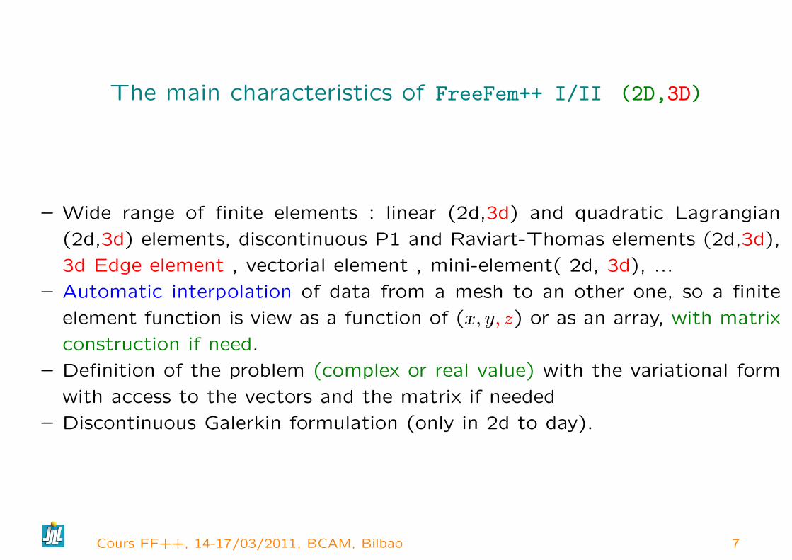
The main characteristics of FreeFem++ I/II (2D,3D)
– Wide range of finite elements : linear (2d,3d) and quadratic Lagrangian
(2d,3d) elements, discontinuous P1 and Raviart-Thomas elements (2d,3d),
3d Edge element , vectorial element , mini-element( 2d, 3d), ...
– Automatic interpolation of data from a mesh to an other one, so a finite
element function is view as a function of (x, y, z) or as an array, with matrix
construction if need.
– Definition of the problem (complex or real value) with the variational form
with access to the vectors and the matrix if needed
– Discontinuous Galerkin formulation (only in 2d to day).
Cours FF++, 14-17/03/2011, BCAM, Bilbao 7
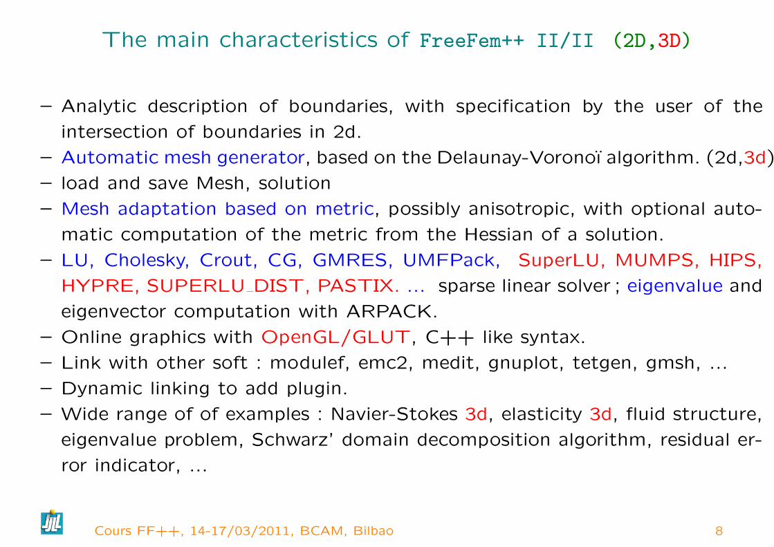
The main characteristics of FreeFem++ II/II (2D,3D)
– Analytic description of boundaries, with specification by the user of the
intersection of boundaries in 2d.
– Automatic mesh generator, based on the Delaunay-Voronoı algorithm. (2d,3d)
– load and save Mesh, solution
– Mesh adaptation based on metric, possibly anisotropic, with optional auto-
matic computation of the metric from the Hessian of a solution.
– LU, Cholesky, Crout, CG, GMRES, UMFPack, SuperLU, MUMPS, HIPS,
HYPRE, SUPERLU DIST, PASTIX. ... sparse linear solver ; eigenvalue and
eigenvector computation with ARPACK.
– Online graphics with OpenGL/GLUT, C++ like syntax.
– Link with other soft : modulef, emc2, medit, gnuplot, tetgen, gmsh, ...
– Dynamic linking to add plugin.
– Wide range of of examples : Navier-Stokes 3d, elasticity 3d, fluid structure,
eigenvalue problem, Schwarz’ domain decomposition algorithm, residual er-
ror indicator, ...
Cours FF++, 14-17/03/2011, BCAM, Bilbao 8
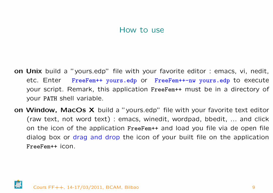
How to use
on Unix build a ”yours.edp” file with your favorite editor : emacs, vi, nedit,
etc. Enter FreeFem++ yours.edp or FreeFem++-nw yours.edp to execute
your script. Remark, this application FreeFem++ must be in a directory of
your PATH shell variable.
on Window, MacOs X build a ”yours.edp” file with your favorite text editor
(raw text, not word text) : emacs, winedit, wordpad, bbedit, ... and click
on the icon of the application FreeFem++ and load you file via de open file
dialog box or drag and drop the icon of your built file on the application
FreeFem++ icon.
Cours FF++, 14-17/03/2011, BCAM, Bilbao 9
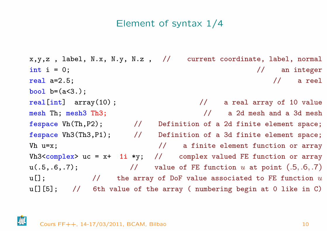
Element of syntax 1/4
x,y,z , label, N.x, N.y, N.z , // current coordinate, label, normal
int i = 0; // an integer
real a=2.5; // a reel
bool b=(a<3.);
real[int] array(10) ; // a real array of 10 value
mesh Th; mesh3 Th3; // a 2d mesh and a 3d mesh
fespace Vh(Th,P2); // Definition of a 2d finite element space;
fespace Vh3(Th3,P1); // Definition of a 3d finite element space;
Vh u=x; // a finite element function or array
Vh3<complex> uc = x+ 1i *y; // complex valued FE function or array
u(.5,.6,.7); // value of FE function u at point (.5, .6, .7)
u[]; // the array of DoF value associated to FE function u
u[][5]; // 6th value of the array ( numbering begin at 0 like in C)
Cours FF++, 14-17/03/2011, BCAM, Bilbao 10

Element of syntax 2/4
fespace V3h(Th,[P2,P2,P1]);
V3h [u1,u2,p]=[x,y,z]; // a vectorial finite element function or array
// remark u1[] <==> u2[] <==> p[] same array of unknown.
macro div(u,v) (dx(u)+dy(v))// EOM a macro (like #define in C )
macro Grad(u) [dx(u),dy(u)]// EOM this end with the comment//
varf a([u1,u2,p],[v1,v2,q])=
int2d(Th)( Grad(u1)’*Grad(v1) +Grad(u2)’*Grad(v2)
-div(u1,u2)*q -div(v1,v2)*p)
+on(1,2)(u1=g1,u2=g2);
matrix A=a(V3h,V3h,solver=UMFPACK);
real[int] b=a(0,V3h);
u2[] =A^-1*b; // or you can put also u1[]= or p[].
Cours FF++, 14-17/03/2011, BCAM, Bilbao 11
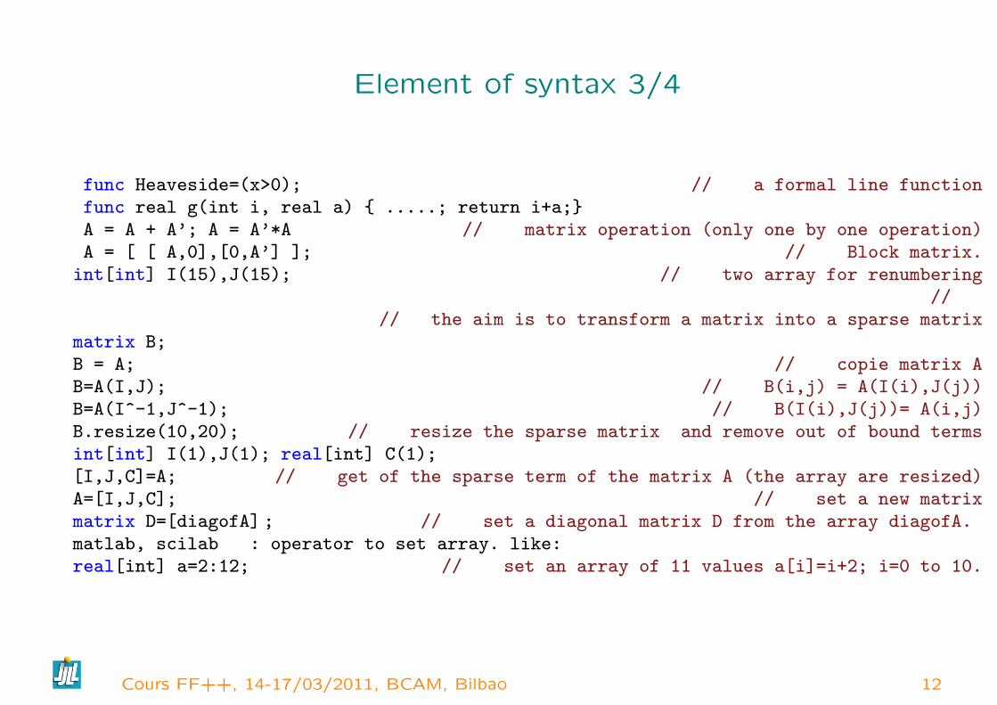
Element of syntax 3/4
func Heaveside=(x>0); // a formal line functionfunc real g(int i, real a) .....; return i+a;A = A + A’; A = A’*A // matrix operation (only one by one operation)A = [ [ A,0],[0,A’] ]; // Block matrix.int[int] I(15),J(15); // two array for renumbering
//// the aim is to transform a matrix into a sparse matrix
matrix B;B = A; // copie matrix AB=A(I,J); // B(i,j) = A(I(i),J(j))B=A(I^-1,J^-1); // B(I(i),J(j))= A(i,j)B.resize(10,20); // resize the sparse matrix and remove out of bound termsint[int] I(1),J(1); real[int] C(1);[I,J,C]=A; // get of the sparse term of the matrix A (the array are resized)A=[I,J,C]; // set a new matrixmatrix D=[diagofA] ; // set a diagonal matrix D from the array diagofA.matlab, scilab : operator to set array. like:real[int] a=2:12; // set an array of 11 values a[i]=i+2; i=0 to 10.
Cours FF++, 14-17/03/2011, BCAM, Bilbao 12
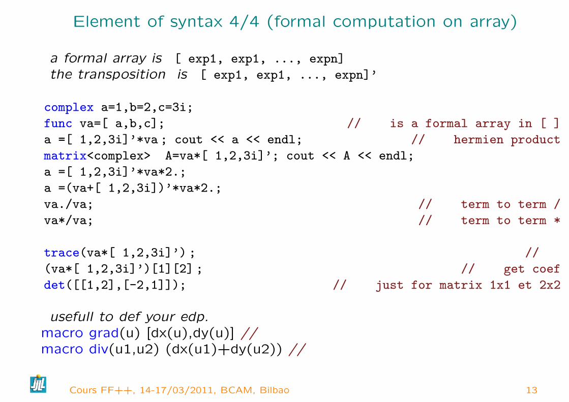
Element of syntax 4/4 (formal computation on array)
a formal array is [ exp1, exp1, ..., expn]
the transposition is [ exp1, exp1, ..., expn]’
complex a=1,b=2,c=3i;
func va=[ a,b,c]; // is a formal array in [ ]
a =[ 1,2,3i]’*va ; cout << a << endl; // hermien product
matrix<complex> A=va*[ 1,2,3i]’; cout << A << endl;
a =[ 1,2,3i]’*va*2.;
a =(va+[ 1,2,3i])’*va*2.;
va./va; // term to term /
va*/va; // term to term *
trace(va*[ 1,2,3i]’) ; //
(va*[ 1,2,3i]’)[1][2] ; // get coef
det([[1,2],[-2,1]]); // just for matrix 1x1 et 2x2
usefull to def your edp.macro grad(u) [dx(u),dy(u)] //macro div(u1,u2) (dx(u1)+dy(u2)) //
Cours FF++, 14-17/03/2011, BCAM, Bilbao 13

Element of syntax : Like in C
The key words are reserved
The operator like in C exempt: ^ & |+ - * / ^ // where a^b= ab
== != < > <= >= & | // where a|b= a or b, a&b= a and b= += -= /= *=
BOOLEAN: 0 <=> false , 6= 0 <=> true = 1
// Automatic cast for numerical value : bool, int, reel, complex , sofunc heavyside = real(x>0.);
for (int i=0;i<n;i++) ... ;if ( <bool exp> ) ... ; else ...;;while ( <bool exp> ) ... ;break continue key words
weakless: all local variables are almost static (????)bug if break before variable declaration in same block.bug for fespace argument or fespace function argument
Cours FF++, 14-17/03/2011, BCAM, Bilbao 14
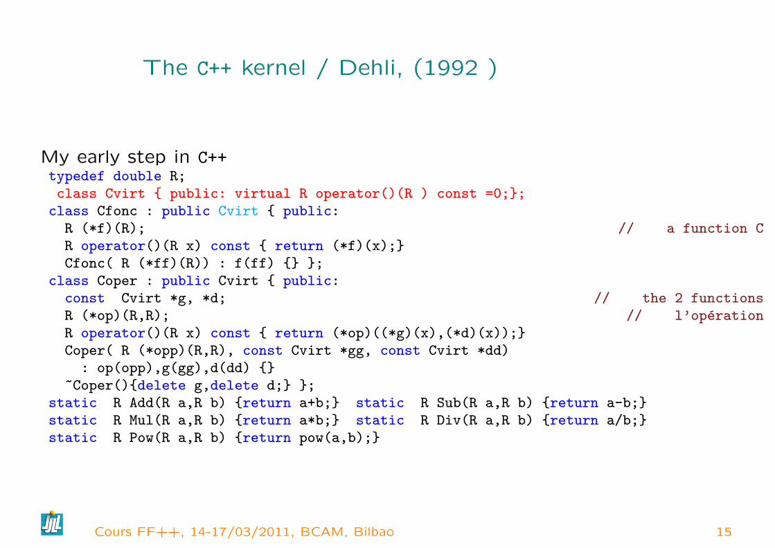
The C++ kernel / Dehli, (1992 ) (Idea, I)
My early step in C++typedef double R;class Cvirt public: virtual R operator()(R ) const =0;;class Cfonc : public Cvirt public:R (*f)(R); // a function CR operator()(R x) const return (*f)(x);Cfonc( R (*ff)(R)) : f(ff) ;
class Coper : public Cvirt public:const Cvirt *g, *d; // the 2 functionsR (*op)(R,R); // l’operationR operator()(R x) const return (*op)((*g)(x),(*d)(x));Coper( R (*opp)(R,R), const Cvirt *gg, const Cvirt *dd): op(opp),g(gg),d(dd)
~Coper()delete g,delete d; ;static R Add(R a,R b) return a+b; static R Sub(R a,R b) return a-b;static R Mul(R a,R b) return a*b; static R Div(R a,R b) return a/b;static R Pow(R a,R b) return pow(a,b);
Cours FF++, 14-17/03/2011, BCAM, Bilbao 15
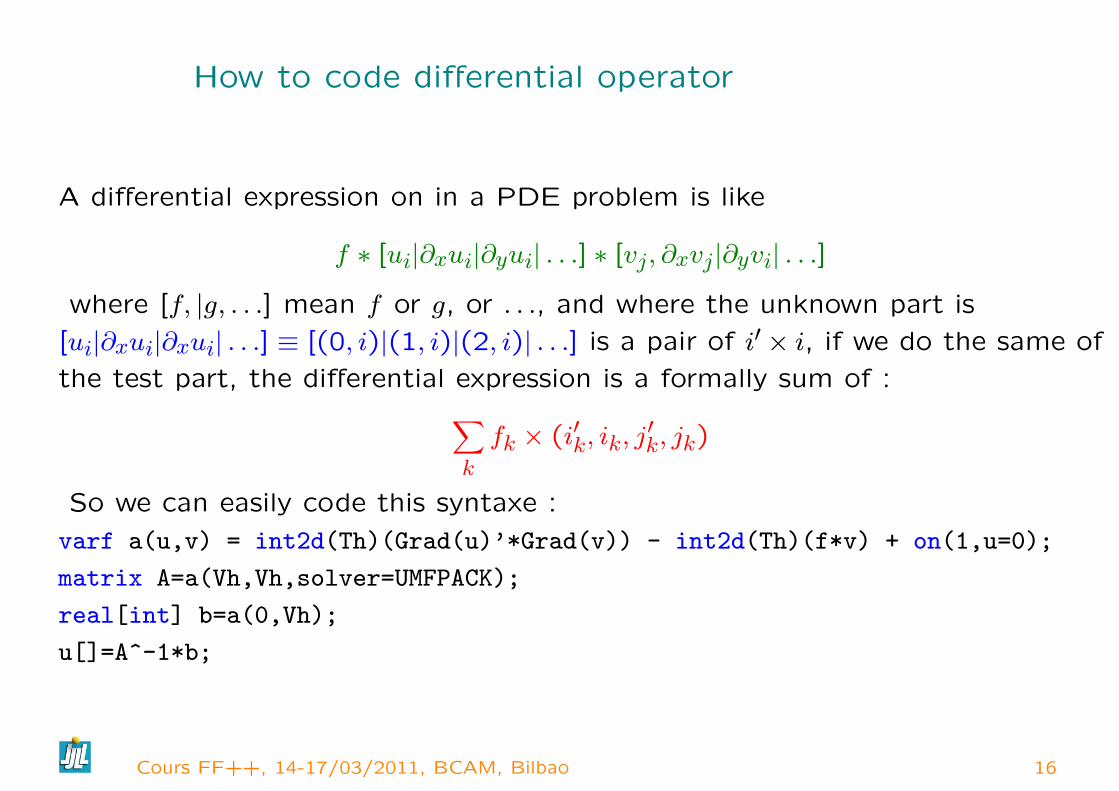
How to code differential operator (Idea, II)
A differential expression on in a PDE problem is like
f ∗ [ui|∂xui|∂yui| . . .] ∗ [vj, ∂xvj|∂yvi| . . .]
where [f, |g, . . .] mean f or g, or . . ., and where the unknown part is
[ui|∂xui|∂xui| . . .] ≡ [(0, i)|(1, i)|(2, i)| . . .] is a pair of i′ × i, if we do the same of
the test part, the differential expression is a formally sum of :∑k
fk × (i′k, ik, j′k, jk)
So we can easily code this syntaxe :
varf a(u,v) = int2d(Th)(Grad(u)’*Grad(v)) - int2d(Th)(f*v) + on(1,u=0);
matrix A=a(Vh,Vh,solver=UMFPACK);
real[int] b=a(0,Vh);
u[]=A^-1*b;
Cours FF++, 14-17/03/2011, BCAM, Bilbao 16

Laplace equation, weak form
Let a domain Ω with a partition of ∂Ω in Γ2,Γe.
Find u a solution in such that :
−∆u = 1 in Ω, u = 2 on Γ2,∂u
∂~n= 0 on Γe (1)
Denote Vg = v ∈ H1(Ω)/v|Γ2= g .
The Basic variationnal formulation with is : find u ∈ V2(Ω) , such that∫Ω∇u.∇v =
∫Ω
1v+∫
Γ
∂u
∂nv, ∀v ∈ V0(Ω) (2)
Cours FF++, 14-17/03/2011, BCAM, Bilbao 17

Laplace equation in FreeFem++
The finite element method is just : replace Vg with a finite element space,
and the FreeFem++ code :
mesh3 Th("Th-hex-sph.msh"); // read a mesh 3d
fespace Vh(Th,P1); // define the P1 EF space
Vh u,v; // set test and unknow FE function in Vh.
macro Grad(u) [dx(u),dy(u),dz(u)] // End of Macro Grad definition
solve laplace(u,v,solver=CG) =
int3d(Th)( Grad(u)’*Grad(v) ) - int3d(Th) ( 1*v)
+ on(2,u=2); // int on γ2
plot(u,fill=1,wait=1,value=0,wait=1);
Cours FF++, 14-17/03/2011, BCAM, Bilbao 18

Laplace equation 2d / figure
Execute fish.edp Execute Laplace3d.edp Execute EqPoisson.edp
Cours FF++, 14-17/03/2011, BCAM, Bilbao 19

Build Mesh 2d
First a 10× 10 grid mesh of unit square ]0,1[2
int[int] labs=[10,20,30,40]; // resp. bottom, right, top, left boundary labelsmesh Th1 = square(10,10,label=labs,region=0); // boundary label:plot(Th1,wait=1);int[int] old2newlabs=[10,11, 30,31]; // the boundary labels 10 in 11 and 30 in 31Th1=change(Th1,label=old2newlabs [,region= old2newregion]); // do Change in 2d or in 3d.
second a L shape domain ]0,1[2\[12,1[2
border a(t=0,1.0)x=t; y=0; label=1;;border b(t=0,0.5)x=1; y=t; label=2;;border c(t=0,0.5)x=1-t; y=0.5;label=3;;border d(t=0.5,1)x=0.5; y=t; label=4;;border e(t=0.5,1)x=1-t; y=1; label=5;;border f(t=0.0,1)x=0; y=1-t;label=6;;plot(a(6) + b(4) + c(4) +d(4) + e(4) + f(6),wait=1); // to see the 6 bordersmesh Th2 = buildmesh (a(6) + b(4) + c(4) +d(4) + e(4) + f(6));
Get a extern meshmesh Th2("april-fish.msh");
build with emc2, bamg, modulef, etc...
Cours FF++, 14-17/03/2011, BCAM, Bilbao 20

a corner singularity adaptation with metric
The domain is an L-shaped polygon Ω =]0,1[2\[12,1]2 and the PDE is
Find u ∈ H10(Ω) such that −∆u = 1 in Ω,
The solution has a singularity at the reentrant angle and we wish to capture
it numerically.
example of Mesh adaptation
Cours FF++, 14-17/03/2011, BCAM, Bilbao 21

FreeFem++ corner singularity program
border a(t=0,1.0)x=t; y=0; label=1;;border b(t=0,0.5)x=1; y=t; label=2;;border c(t=0,0.5)x=1-t; y=0.5;label=3;;border d(t=0.5,1)x=0.5; y=t; label=4;;border e(t=0.5,1)x=1-t; y=1; label=5;;border f(t=0.0,1)x=0; y=1-t;label=6;;
mesh Th = buildmesh (a(6) + b(4) + c(4) +d(4) + e(4) + f(6));fespace Vh(Th,P1); Vh u,v; real error=0.01;problem Probem1(u,v,solver=CG,eps=1.0e-6) =
int2d(Th)( dx(u)*dx(v) + dy(u)*dy(v)) - int2d(Th)( v)+ on(1,2,3,4,5,6,u=0);
int i;for (i=0;i< 7;i++) Probem1; // solving the pde problem
Th=adaptmesh(Th,u,err=error); // the adaptation with Hessian of uplot(Th,wait=1); u=u; error = error/ (1000^(1./7.)) ; ;
Execute adapt.edp
Cours FF++, 14-17/03/2011, BCAM, Bilbao 22
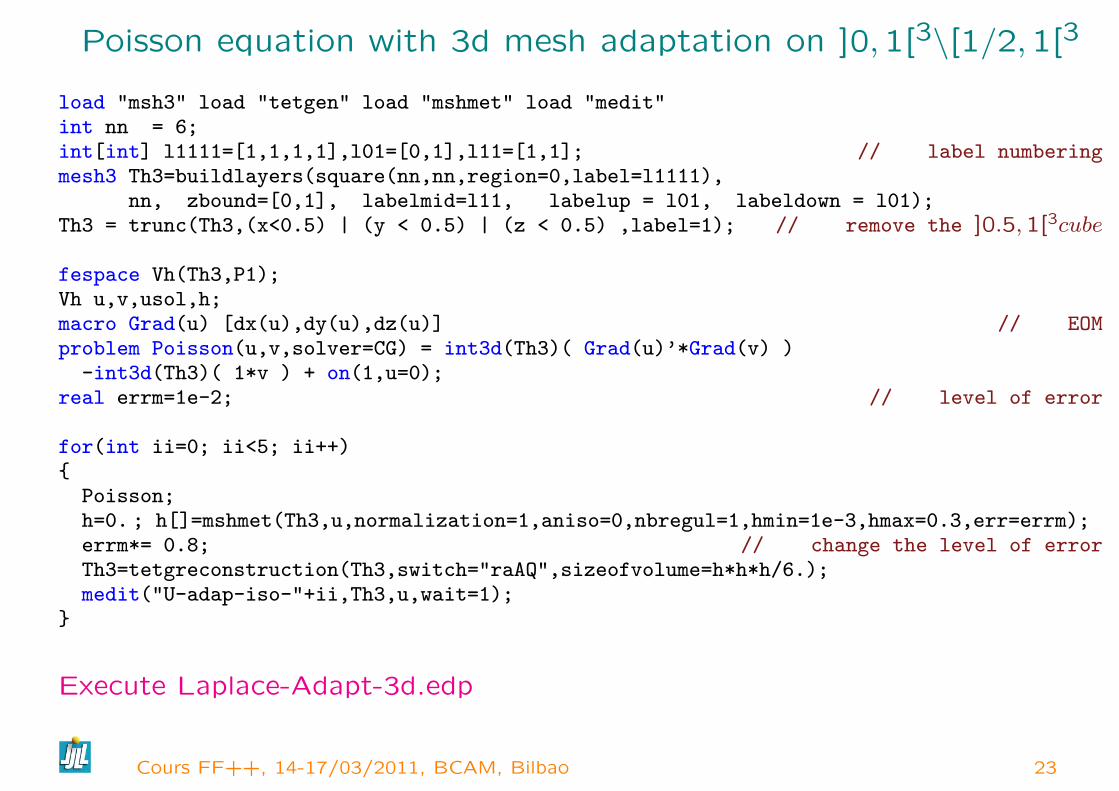
Poisson equation with 3d mesh adaptation on ]0,1[3\[1/2,1[3
load "msh3" load "tetgen" load "mshmet" load "medit"int nn = 6;int[int] l1111=[1,1,1,1],l01=[0,1],l11=[1,1]; // label numberingmesh3 Th3=buildlayers(square(nn,nn,region=0,label=l1111),
nn, zbound=[0,1], labelmid=l11, labelup = l01, labeldown = l01);Th3 = trunc(Th3,(x<0.5) | (y < 0.5) | (z < 0.5) ,label=1); // remove the ]0.5,1[3cube
fespace Vh(Th3,P1);Vh u,v,usol,h;macro Grad(u) [dx(u),dy(u),dz(u)] // EOMproblem Poisson(u,v,solver=CG) = int3d(Th3)( Grad(u)’*Grad(v) )-int3d(Th3)( 1*v ) + on(1,u=0);
real errm=1e-2; // level of error
for(int ii=0; ii<5; ii++)Poisson;h=0. ; h[]=mshmet(Th3,u,normalization=1,aniso=0,nbregul=1,hmin=1e-3,hmax=0.3,err=errm);errm*= 0.8; // change the level of errorTh3=tetgreconstruction(Th3,switch="raAQ",sizeofvolume=h*h*h/6.);medit("U-adap-iso-"+ii,Th3,u,wait=1);
Execute Laplace-Adapt-3d.edp
Cours FF++, 14-17/03/2011, BCAM, Bilbao 23

A cube with buildlayer (simple)
load "msh3" // buildlayer
int nn=10;
int[int]
rup=[0,2], // label of the upper face 0-> 2 (region -> label)
rdown=[0,1], // label of the lower face 0-> 1 (region -> label)
rmid=[1,1 ,2,1 ,3,1 ,4,1 ], // 4 Vert. faces: 2d label -> 3d label
rtet[0,0];
real zmin=0,zmax=1;
mesh3 Th=buildlayers(square(nn,nn,),nn,
zbound=[zmin,zmax],
labeltet=rtet,
labelmid=rmid,
labelup = rup,
labeldown = rdown);
Execute Cube.edp
Cours FF++, 14-17/03/2011, BCAM, Bilbao 24
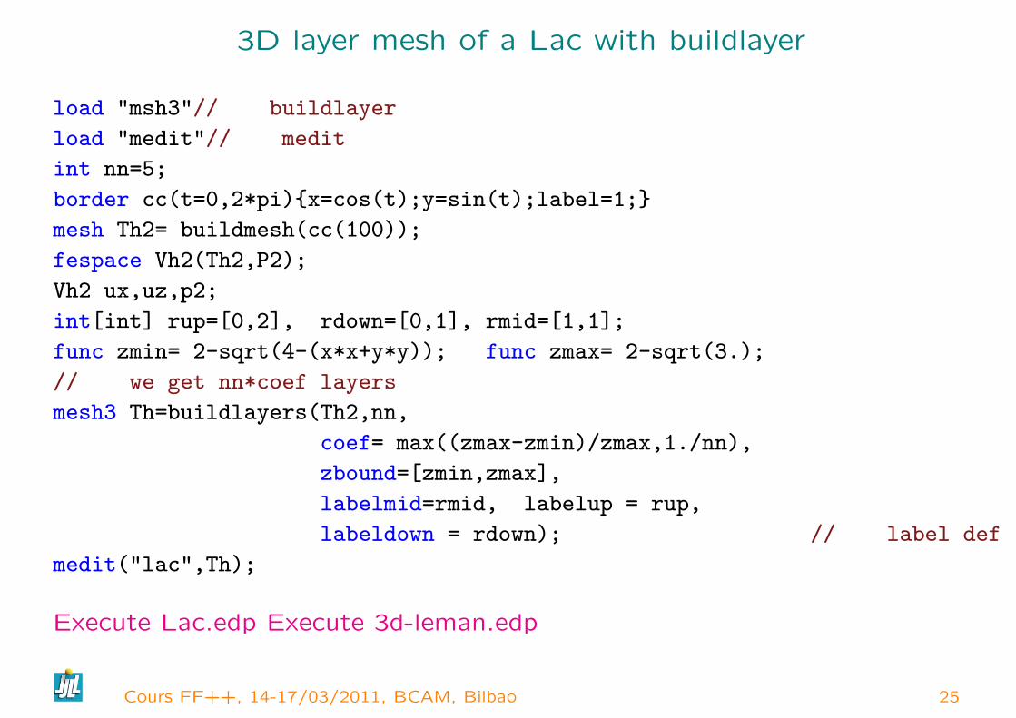
3D layer mesh of a Lac with buildlayer
load "msh3"// buildlayer
load "medit"// medit
int nn=5;
border cc(t=0,2*pi)x=cos(t);y=sin(t);label=1;
mesh Th2= buildmesh(cc(100));
fespace Vh2(Th2,P2);
Vh2 ux,uz,p2;
int[int] rup=[0,2], rdown=[0,1], rmid=[1,1];
func zmin= 2-sqrt(4-(x*x+y*y)); func zmax= 2-sqrt(3.);
// we get nn*coef layers
mesh3 Th=buildlayers(Th2,nn,
coef= max((zmax-zmin)/zmax,1./nn),
zbound=[zmin,zmax],
labelmid=rmid, labelup = rup,
labeldown = rdown); // label def
medit("lac",Th);
Execute Lac.edp Execute 3d-leman.edp
Cours FF++, 14-17/03/2011, BCAM, Bilbao 25
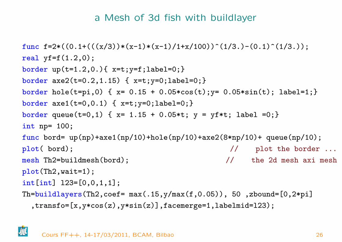
a Mesh of 3d fish with buildlayer
func f=2*((0.1+(((x/3))*(x-1)*(x-1)/1+x/100))^(1/3.)-(0.1)^(1/3.));
real yf=f(1.2,0);
border up(t=1.2,0.) x=t;y=f;label=0;
border axe2(t=0.2,1.15) x=t;y=0;label=0;
border hole(t=pi,0) x= 0.15 + 0.05*cos(t);y= 0.05*sin(t); label=1;
border axe1(t=0,0.1) x=t;y=0;label=0;
border queue(t=0,1) x= 1.15 + 0.05*t; y = yf*t; label =0;
int np= 100;
func bord= up(np)+axe1(np/10)+hole(np/10)+axe2(8*np/10)+ queue(np/10);
plot( bord); // plot the border ...
mesh Th2=buildmesh(bord); // the 2d mesh axi mesh
plot(Th2,wait=1);
int[int] l23=[0,0,1,1];
Th=buildlayers(Th2,coef= max(.15,y/max(f,0.05)), 50 ,zbound=[0,2*pi]
,transfo=[x,y*cos(z),y*sin(z)],facemerge=1,labelmid=l23);
Cours FF++, 14-17/03/2011, BCAM, Bilbao 26

boundary mesh of a Sphere
load "tetgen"
mesh Th=square(10,20,[x*pi-pi/2,2*y*pi]); // ]−pi2, −pi
2[×]0,2π[
func f1 =cos(x)*cos(y); func f2 =cos(x)*sin(y); func f3 = sin(x);// the partiel derivative of the parametrization DF
func f1x=sin(x)*cos(y); func f1y=-cos(x)*sin(y);func f2x=-sin(x)*sin(y); func f2y=cos(x)*cos(y);func f3x=cos(x); func f3y=0;
// M = DF tDFfunc m11=f1x^2+f2x^2+f3x^2; func m21=f1x*f1y+f2x*f2y+f3x*f3y;func m22=f1y^2+f2y^2+f3y^2;func perio=[[4,y],[2,y],[1,x],[3,x]];real hh=0.1/R; real vv= 1/square(hh);Th=adaptmesh(Th,m11*vv,m21*vv,m22*vv,IsMetric=1,periodic=perio); // 4 timesint[int] ref=[0,L]; // to set the label of the Sphere to L ( 0 -> L)mesh3 ThS= movemesh23(Th,transfo=[f1*R,f2*R,f3*R],orientation=1,label=ref);
Execute Sphere.edp Execute sphere6.edp
Cours FF++, 14-17/03/2011, BCAM, Bilbao 27

Build 3d Mesh from boundary mesh
include "MeshSurface.idp" // tool for 3d surfaces meshes
mesh3 Th;
try Th=readmesh3("Th-hex-sph.mesh"); // try to read
catch(...) // catch an error dering reading so build the mesh...
real hs = 0.2; // mesh size on sphere
int[int] NN=[11,9,10];
real [int,int] BB=[[-1.1,1.1],[-.9,.9],[-1,1]]; // Mesh Box
int [int,int] LL=[[1,2],[3,4],[5,6]]; // Label Box
mesh3 ThHS = SurfaceHex(NN,BB,LL,1)+Sphere(0.5,hs,7,1); // "gluing"
// surface meshes
real voltet=(hs^3)/6.; // volume mesh control.
real[int] domaine = [0,0,0,1,voltet,0,0,0.7,2,voltet];
Th = tetg(ThHS,switch="pqaAAYYQ",nbofregions=2,regionlist=domaine);
savemesh(Th,"Th-hex-sph.mesh"); // save une mesh for next run
Cours FF++, 14-17/03/2011, BCAM, Bilbao 28
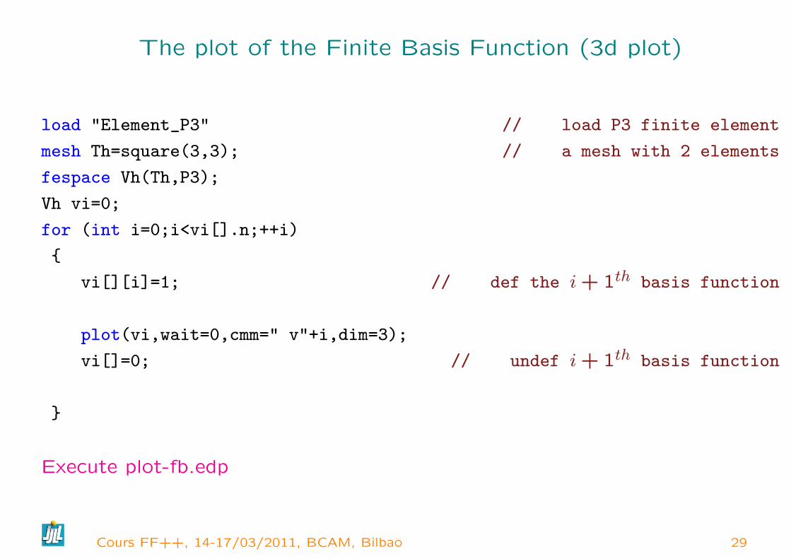
The plot of the Finite Basis Function (3d plot)
load "Element_P3" // load P3 finite element
mesh Th=square(3,3); // a mesh with 2 elements
fespace Vh(Th,P3);
Vh vi=0;
for (int i=0;i<vi[].n;++i)
vi[][i]=1; // def the i+ 1th basis function
plot(vi,wait=0,cmm=" v"+i,dim=3);
vi[]=0; // undef i+ 1th basis function
Execute plot-fb.edp
Cours FF++, 14-17/03/2011, BCAM, Bilbao 29
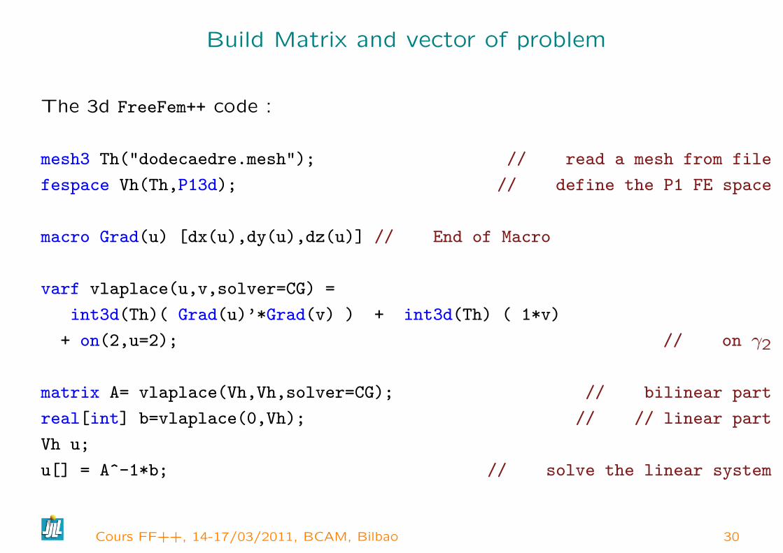
Build Matrix and vector of problem
The 3d FreeFem++ code :
mesh3 Th("dodecaedre.mesh"); // read a mesh from file
fespace Vh(Th,P13d); // define the P1 FE space
macro Grad(u) [dx(u),dy(u),dz(u)] // End of Macro
varf vlaplace(u,v,solver=CG) =
int3d(Th)( Grad(u)’*Grad(v) ) + int3d(Th) ( 1*v)
+ on(2,u=2); // on γ2
matrix A= vlaplace(Vh,Vh,solver=CG); // bilinear part
real[int] b=vlaplace(0,Vh); // // linear part
Vh u;
u[] = A^-1*b; // solve the linear system
Cours FF++, 14-17/03/2011, BCAM, Bilbao 30

Remark on varf
The functions appearing in the variational form are formal and local to thevarf definition, the only important think is the order in the parameter list,like invarf vb1([u1,u2],[q]) = int2d(Th)( (dy(u1)+dy(u2)) *q) + int2d(Th)(1*q);
varf vb2([v1,v2],[p]) = int2d(Th)( (dy(v1)+dy(v2)) *p) + int2d(Th)(1*p);
To build matrix A from the bilinear part the the variational form a of typevarf do simplymatrix B1 = vb1(Vh,Wh [, ...] );matrix<complex> C1 = vb1(Vh,Wh [, ...] );
// where the fespace have the correct number of component// Vh is "fespace" for the unknown fields with 2 component// ex fespace Vh(Th,[P2,P2]); or fespace Vh(Th,RT);// Wh is "fespace" for the test fields with 1 component
To build a vector, put u1 = u2 = 0 by setting 0 of on unknown part.real[int] b = vb2(0,Wh);
complex[int] c = vb2(0,Wh);
Remark : In this case the mesh use to defined ,∫, u, v can be different.
Cours FF++, 14-17/03/2011, BCAM, Bilbao 31
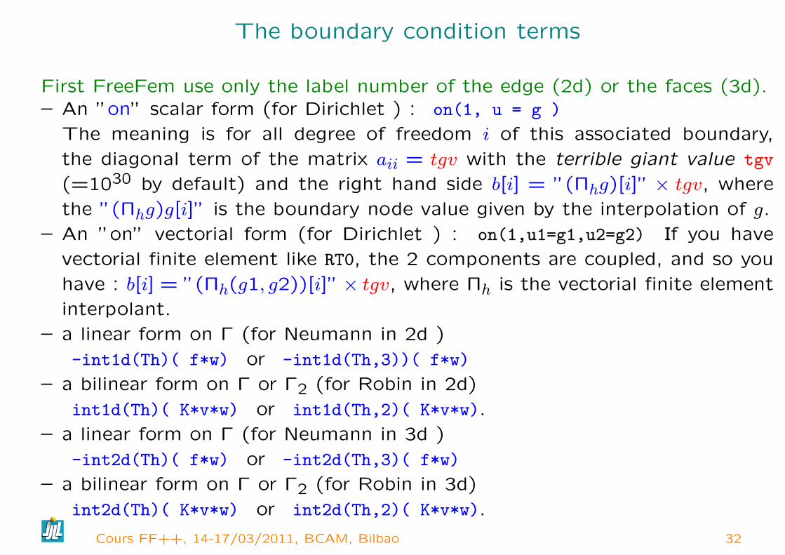
The boundary condition terms
First FreeFem use only the label number of the edge (2d) or the faces (3d).– An ”on” scalar form (for Dirichlet ) : on(1, u = g )
The meaning is for all degree of freedom i of this associated boundary,
the diagonal term of the matrix aii = tgv with the terrible giant value tgv
(=1030 by default) and the right hand side b[i] = ”(Πhg)[i]” × tgv, where
the ”(Πhg)g[i]” is the boundary node value given by the interpolation of g.
– An ”on” vectorial form (for Dirichlet ) : on(1,u1=g1,u2=g2) If you have
vectorial finite element like RT0, the 2 components are coupled, and so you
have : b[i] = ”(Πh(g1, g2))[i]”× tgv, where Πh is the vectorial finite element
interpolant.
– a linear form on Γ (for Neumann in 2d )
-int1d(Th)( f*w) or -int1d(Th,3))( f*w)
– a bilinear form on Γ or Γ2 (for Robin in 2d)
int1d(Th)( K*v*w) or int1d(Th,2)( K*v*w).
– a linear form on Γ (for Neumann in 3d )
-int2d(Th)( f*w) or -int2d(Th,3)( f*w)
– a bilinear form on Γ or Γ2 (for Robin in 3d)
int2d(Th)( K*v*w) or int2d(Th,2)( K*v*w).
Cours FF++, 14-17/03/2011, BCAM, Bilbao 32

a Neumann Poisson Problem with 1D Lagrange multiplier
The variationnal form is find (u, λ) ∈ Vh × R such that
∀(v, µ) ∈ Vh × R a(u, v) + b(u, µ) + b(v, λ) = l(v), where b(u, µ) =∫µudx
mesh Th=square(10,10); fespace Vh(Th,P1); // P1 FE space
int n = Vh.ndof, n1 = n+1;
func f=1+x-y; macro Grad(u) [dx(u),dy(u)] // EOM
varf va(uh,vh) = int2d(Th)( Grad(uh)’*Grad(vh) ) ;
varf vL(uh,vh) = int2d(Th)( f*vh ) ; varf vb(uh,vh)= int2d(Th)(1.*vh);
matrix A=va(Vh,Vh);
real[int] b=vL(0,Vh), B = vb(0,Vh);
real[int] bb(n1),x(n1),b1(1),l(1); b1=0;
matrix AA = [ [ A , B ] , [ B’, 0 ] ] ; bb = [ b, b1]; // blocks
set(AA,solver=UMFPACK); // set the type of linear solver.
x = AA^-1*bb; [uh[],l] = x; // solve the linear system
plot(uh,wait=1); // set the value
Execute Laplace-lagrange-mult.edp
Cours FF++, 14-17/03/2011, BCAM, Bilbao 33
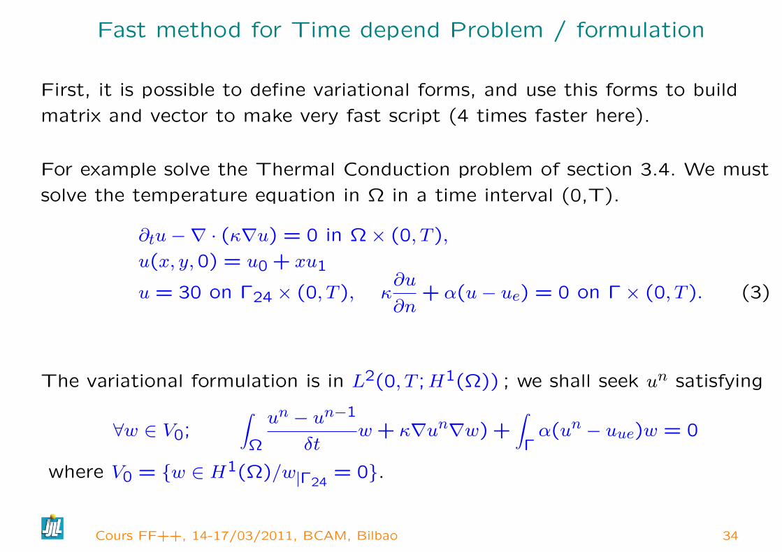
Fast method for Time depend Problem / formulation
First, it is possible to define variational forms, and use this forms to build
matrix and vector to make very fast script (4 times faster here).
For example solve the Thermal Conduction problem of section 3.4. We must
solve the temperature equation in Ω in a time interval (0,T).
∂tu−∇ · (κ∇u) = 0 in Ω× (0, T ),
u(x, y,0) = u0 + xu1
u = 30 on Γ24 × (0, T ), κ∂u
∂n+ α(u− ue) = 0 on Γ× (0, T ). (3)
The variational formulation is in L2(0, T ;H1(Ω)) ; we shall seek un satisfying
∀w ∈ V0;∫
Ω
un − un−1
δtw + κ∇un∇w) +
∫Γα(un − uue)w = 0
where V0 = w ∈ H1(Ω)/w|Γ24= 0.
Cours FF++, 14-17/03/2011, BCAM, Bilbao 34
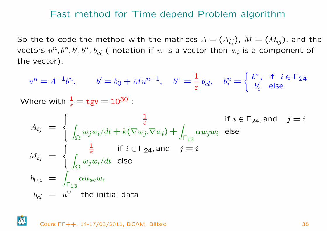
Fast method for Time depend Problem algorithm
So the to code the method with the matrices A = (Aij), M = (Mij), and the
vectors un, bn, b′, b”, bcl ( notation if w is a vector then wi is a component of
the vector).
un = A−1bn, b′ = b0 +Mun−1, b” =1
εbcl, bni =
b”i if i ∈ Γ24b′i else
Where with 1ε = tgv = 1030 :
Aij =
1ε if i ∈ Γ24, and j = i∫
Ωwjwi/dt+ k(∇wj.∇wi) +
∫Γ13
αwjwi else
Mij =
1ε if i ∈ Γ24, and j = i∫
Ωwjwi/dt else
b0,i =∫
Γ13
αuuewi
bcl = u0 the initial data
Cours FF++, 14-17/03/2011, BCAM, Bilbao 35

Fast The Time depend Problem/ edp
...
Vh u0=fu0,u=u0;
Create three variational formulation, and build the matrices A,M .
varf vthermic (u,v)= int2d(Th)(u*v/dt + k*(dx(u) * dx(v) + dy(u) * dy(v)))
+ int1d(Th,1,3)(alpha*u*v) + on(2,4,u=1);
varf vthermic0(u,v) = int1d(Th,1,3)(alpha*ue*v);
varf vMass (u,v)= int2d(Th)( u*v/dt) + on(2,4,u=1);
real tgv = 1e30;
A= vthermic(Vh,Vh,tgv=tgv,solver=CG);
matrix M= vMass(Vh,Vh);
Cours FF++, 14-17/03/2011, BCAM, Bilbao 36
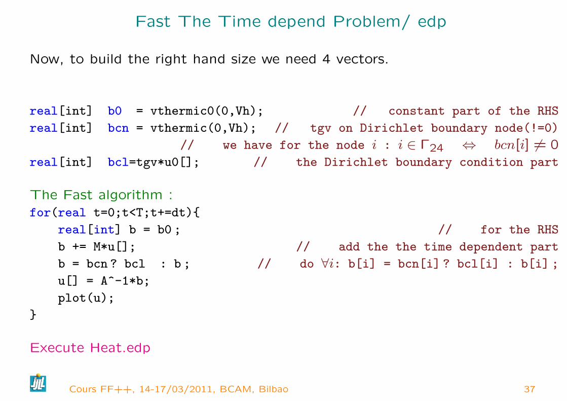
Fast The Time depend Problem/ edp
Now, to build the right hand size we need 4 vectors.
real[int] b0 = vthermic0(0,Vh); // constant part of the RHS
real[int] bcn = vthermic(0,Vh); // tgv on Dirichlet boundary node(!=0)
// we have for the node i : i ∈ Γ24 ⇔ bcn[i] 6= 0real[int] bcl=tgv*u0[]; // the Dirichlet boundary condition part
The Fast algorithm :for(real t=0;t<T;t+=dt)
real[int] b = b0 ; // for the RHS
b += M*u[]; // add the the time dependent part
b = bcn ? bcl : b ; // do ∀i: b[i] = bcn[i] ? bcl[i] : b[i] ;
u[] = A^-1*b;
plot(u);
Execute Heat.edp
Cours FF++, 14-17/03/2011, BCAM, Bilbao 37
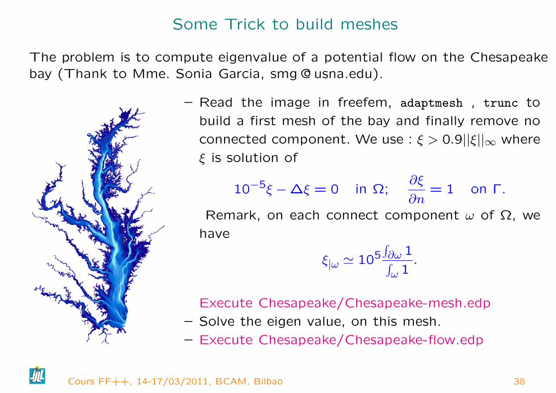
Some Trick to build meshes
The problem is to compute eigenvalue of a potential flow on the Chesapeakebay (Thank to Mme. Sonia Garcia, smg @ usna.edu).
– Read the image in freefem, adaptmesh , trunc to
build a first mesh of the bay and finally remove no
connected component. We use : ξ > 0.9||ξ||∞ where
ξ is solution of
10−5ξ −∆ξ = 0 in Ω;∂ξ
∂n= 1 on Γ.
Remark, on each connect component ω of Ω, we
have
ξ|ω ' 105∫∂ω 1∫ω 1
.
Execute Chesapeake/Chesapeake-mesh.edp
– Solve the eigen value, on this mesh.
– Execute Chesapeake/Chesapeake-flow.edp
Cours FF++, 14-17/03/2011, BCAM, Bilbao 38
Error indicator
For the Laplace problem
−∆u = f in Ω, u = g on ∂Ω
the classical error ηK indicator [C. Bernardi, R. Verfurth] are :
ηK =∫Kh2K|(f + ∆uh)|2 +
∫∂K
he|[∂uh∂n
]|2
where hK is size of the longest edge, he is the size of the current edge, n the
normal.
Theorem : This indicator is optimal with Lagrange Finite element
c0
√∑K
η2K ≤ ||u− uh||H1
≤ c1√∑K
η2K
where c0 and c1 are two constant independent of h , if Th is a regular family
of triangulation.
Cours FF++, 14-17/03/2011, BCAM, Bilbao 39
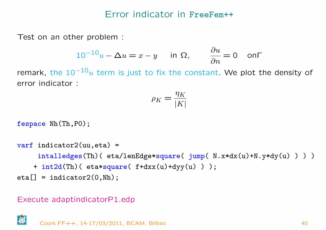
Error indicator in FreeFem++
Test on an other problem :
10−10u−∆u = x− y in Ω,∂u
∂n= 0 onΓ
remark, the 10−10u term is just to fix the constant. We plot the density of
error indicator :
ρK =ηK|K|
fespace Nh(Th,P0);
varf indicator2(uu,eta) =
intalledges(Th)( eta/lenEdge*square( jump( N.x*dx(u)+N.y*dy(u) ) ) )
+ int2d(Th)( eta*square( f+dxx(u)+dyy(u) ) );
eta[] = indicator2(0,Nh);
Execute adaptindicatorP1.edp
Cours FF++, 14-17/03/2011, BCAM, Bilbao 40
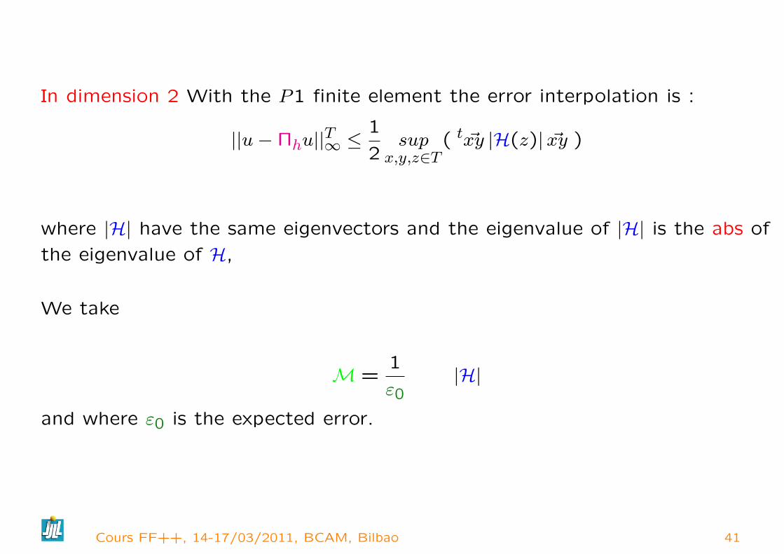
In dimension 2 With the P1 finite element the error interpolation is :
||u−Πhu||T∞ ≤1
2sup
x,y,z∈T( t ~xy |H(z)| ~xy )
where |H| have the same eigenvectors and the eigenvalue of |H| is the abs of
the eigenvalue of H,
We take
M =1
ε0|H|
and where ε0 is the expected error.
Cours FF++, 14-17/03/2011, BCAM, Bilbao 41

The mesh with
u = yx2 + y3
+ tanh(10 (sin(5y)− 2x)),
and
M = 50 |H(u)| so
ε0 = 1100
Cours FF++, 14-17/03/2011, BCAM, Bilbao 42
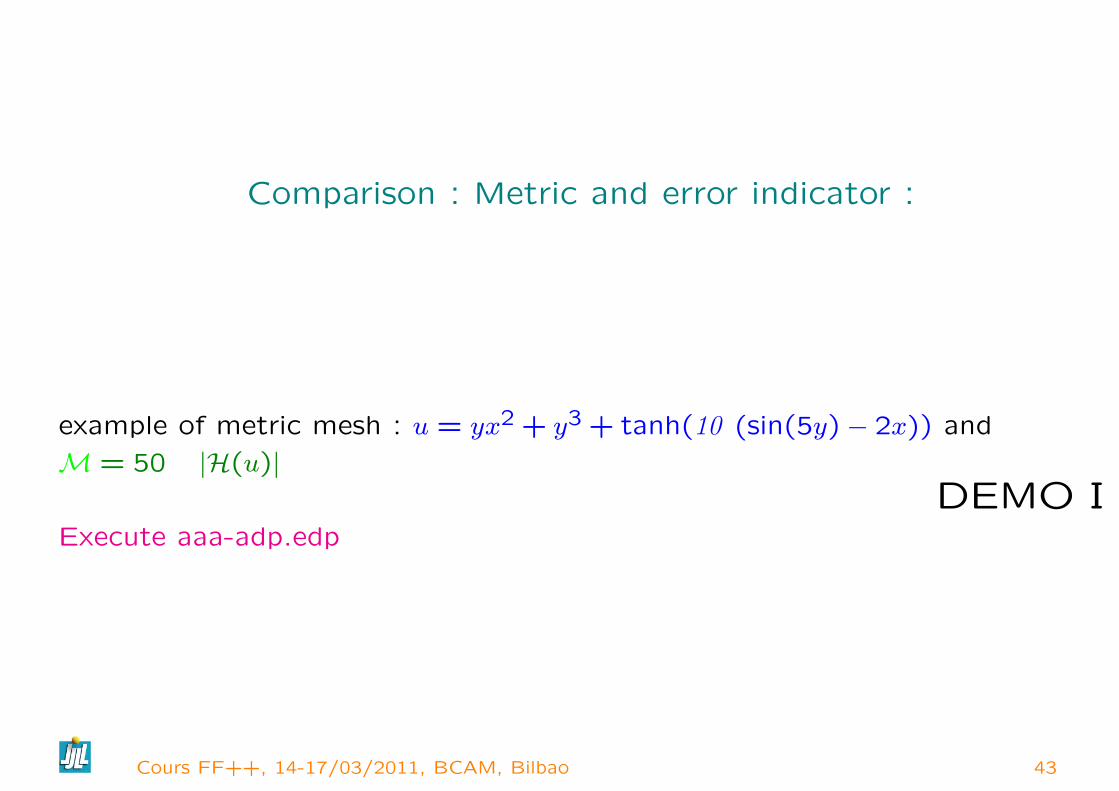
Comparison : Metric and error indicator :
example of metric mesh : u = yx2 + y3 + tanh(10 (sin(5y)− 2x)) and
M = 50 |H(u)|DEMO I
Execute aaa-adp.edp
Cours FF++, 14-17/03/2011, BCAM, Bilbao 43

An academic problem
We propose the solve the following non-linear academic problem of
minimization of a functional
J(u) =1
2
∫Ωf(|∇u|2)− u ∗ b
where u is function of H10(Ω). and where f is defined by
f(x) = a ∗ x+ x− ln(1 + x), f ′(x) = a+x
1 + x, f ′′(x) =
1
(1 + x)2
Cours FF++, 14-17/03/2011, BCAM, Bilbao 44
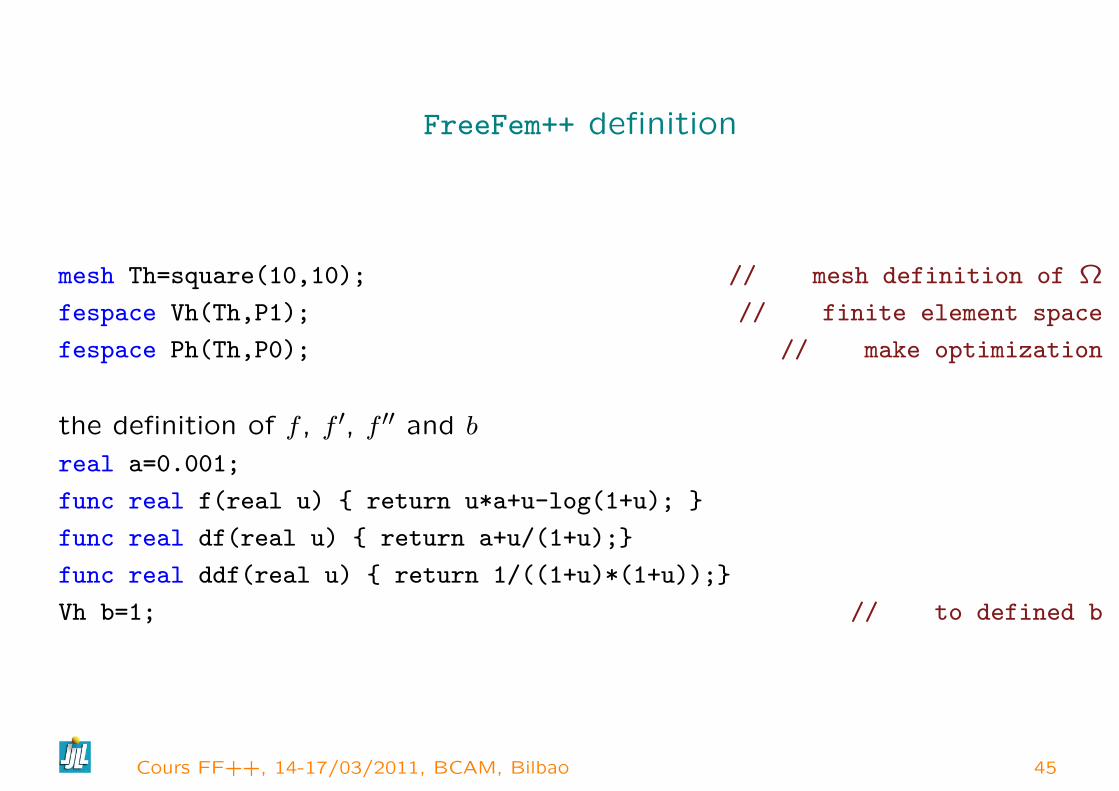
FreeFem++ definition
mesh Th=square(10,10); // mesh definition of Ω
fespace Vh(Th,P1); // finite element space
fespace Ph(Th,P0); // make optimization
the definition of f , f ′, f ′′ and b
real a=0.001;
func real f(real u) return u*a+u-log(1+u);
func real df(real u) return a+u/(1+u);
func real ddf(real u) return 1/((1+u)*(1+u));
Vh b=1; // to defined b
Cours FF++, 14-17/03/2011, BCAM, Bilbao 45
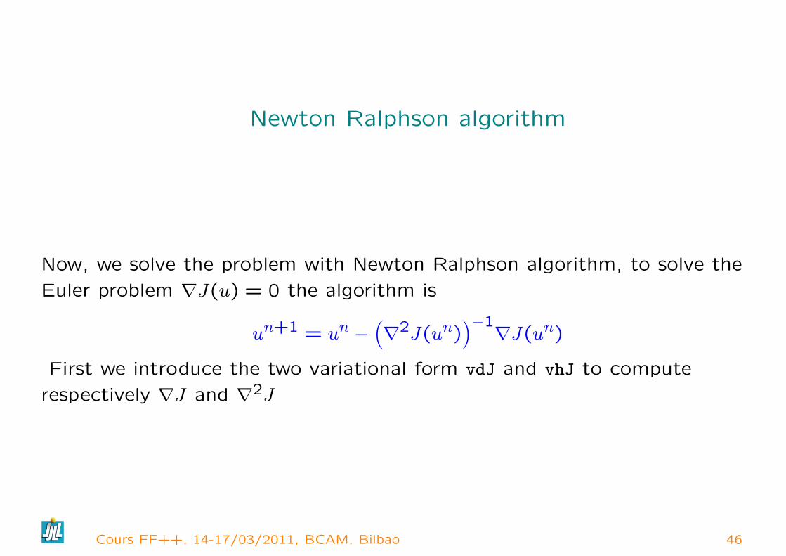
Newton Ralphson algorithm
Now, we solve the problem with Newton Ralphson algorithm, to solve the
Euler problem ∇J(u) = 0 the algorithm is
un+1 = un −(∇2J(un)
)−1∇J(un)
First we introduce the two variational form vdJ and vhJ to compute
respectively ∇J and ∇2J
Cours FF++, 14-17/03/2011, BCAM, Bilbao 46

The variational form
Ph ddfu,dfu ; // to store f ′(|∇u|2) and 2f ′′(|∇u|2) optimization
// the variational form of evaluate dJ = ∇J// --------------------------------------
// dJ = f’()*( dx(u)*dx(vh) + dy(u)*dy(vh)
varf vdJ(uh,vh) = int2d(Th)( dfu *( dx(u)*dx(vh) + dy(u)*dy(vh) ) - b*vh)
+ on(1,2,3,4, uh=0);
// the variational form of evaluate ddJ = ∇2J
// hJ(uh,vh) = f’()*( dx(uh)*dx(vh) + dy(uh)*dy(vh)
// + f’’()( dx(u)*dx(uh) + dy(u)*dy(uh) )
// * (dx(u)*dx(vh) + dy(u)*dy(vh))
varf vhJ(uh,vh) = int2d(Th)( dfu *( dx(uh)*dx(vh) + dy(uh)*dy(vh) )
+ ddfu *(dx(u)*dx(vh) + dy(u)*dy(vh) )*(dx(u)*dx(uh) + dy(u)*dy(uh)))
+ on(1,2,3,4, uh=0);
Cours FF++, 14-17/03/2011, BCAM, Bilbao 47

Newton Ralphson algorithm, next
// the Newton algorithm
Vh v,w;
u=0;
for (int i=0;i<100;i++)
dfu = df( dx(u)*dx(u) + dy(u)*dy(u) ) ; // optimization
ddfu = 2.*ddf( dx(u)*dx(u) + dy(u)*dy(u) ) ; // optimization
v[]= vdJ(0,Vh); // v = ∇J(u), v[] is the array of v
real res= v[]’*v[]; // the dot product
cout << i << " residu^2 = " << res << endl;
if( res< 1e-12) break;
matrix H= vhJ(Vh,Vh,factorize=1,solver=LU); // build and factorize
w[]=H^-1*v[]; // solve the linear system
u[] -= w[];
plot (u,wait=1,cmm="solution with Newton Ralphson");
Execute Newton.edp
Cours FF++, 14-17/03/2011, BCAM, Bilbao 48
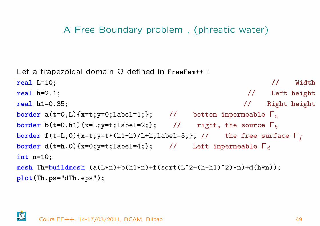
A Free Boundary problem , (phreatic water)
Let a trapezoidal domain Ω defined in FreeFem++ :
real L=10; // Width
real h=2.1; // Left height
real h1=0.35; // Right height
border a(t=0,L)x=t;y=0;label=1;; // bottom impermeable Γaborder b(t=0,h1)x=L;y=t;label=2;; // right, the source Γbborder f(t=L,0)x=t;y=t*(h1-h)/L+h;label=3;; // the free surface Γfborder d(t=h,0)x=0;y=t;label=4;; // Left impermeable Γdint n=10;
mesh Th=buildmesh (a(L*n)+b(h1*n)+f(sqrt(L^2+(h-h1)^2)*n)+d(h*n));
plot(Th,ps="dTh.eps");
Cours FF++, 14-17/03/2011, BCAM, Bilbao 49
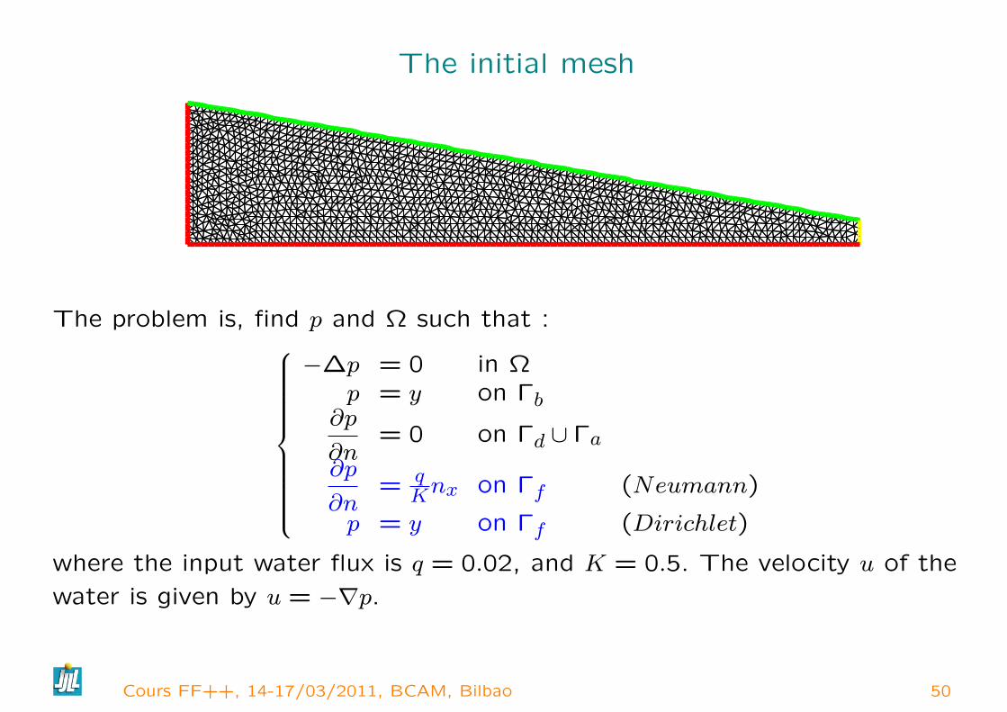
The initial mesh
The problem is, find p and Ω such that :
−∆p = 0 in Ωp = y on Γb
∂p
∂n= 0 on Γd ∪ Γa
∂p
∂n= q
Knx on Γf (Neumann)
p = y on Γf (Dirichlet)
where the input water flux is q = 0.02, and K = 0.5. The velocity u of the
water is given by u = −∇p.
Cours FF++, 14-17/03/2011, BCAM, Bilbao 50
algorithm
We use the following fix point method : let be, k = 0, Ωk = Ω. First step, we
forgot the Neumann BC and we solve the problem : Find p in V = H1(Ωk),
such p = y onon Γkb et on Γkf∫Ωk∇p∇p′ = 0, ∀p′ ∈ V with p′ = 0 on Γkb ∪ Γkf
With the residual of the Neumann boundary condition we build a domain
transformation F(x, y) = [x, y − v(x)] where v is solution of : v ∈ V , such than
v = 0 on Γka (bottom)∫Ωk∇v∇v′ =
∫Γkf
(∂p
∂n−q
Knx)v′, ∀v′ ∈ V with v′ = 0 sur Γka
remark : we can use the previous equation to evaluate∫Γk
∂p
∂nv′ = −
∫Ωk∇p∇v′
Cours FF++, 14-17/03/2011, BCAM, Bilbao 51

The new domain is : Ωk+1 = F(Ωk) Warning if is the movement is too large
we can have triangle overlapping.
problem Pp(p,pp,solver=CG) = int2d(Th)( dx(p)*dx(pp)+dy(p)*dy(pp))
+ on(b,f,p=y) ;
problem Pv(v,vv,solver=CG) = int2d(Th)( dx(v)*dx(vv)+dy(v)*dy(vv))
+ on (a, v=0) + int1d(Th,f)(vv*((Q/K)*N.y- (dx(p)*N.x+dy(p)*N.y)));
while(errv>1e-6)
j++; Pp; Pv; errv=int1d(Th,f)(v*v);
coef = 1;
// Here french cooking if overlapping see the example
Th=movemesh(Th,[x,y-coef*v]); // deformation
Execute freeboundary.edp
Cours FF++, 14-17/03/2011, BCAM, Bilbao 52

Eigenvalue/ Eigenvector example
The problem, Find the first λ, uλ such that :
a(uλ, v) =∫
Ω∇uλ∇v = λ
∫Ωuλv = λb(uλ, v)
the boundary condition is make with exact penalization : we put 1e30 = tgv
on the diagonal term of the lock degree of freedom. So take Dirichlet
boundary condition only with a variational form and not on b variational form
, because we compute eigenvalue of
w = A−1Bv
Cours FF++, 14-17/03/2011, BCAM, Bilbao 53

Eigenvalue/ Eigenvector example code
...
fespace Vh(Th,P1);
macro Grad(u) [dx(u),dy(u),dz(u)] // EOM
varf a(u1,u2)= int3d(Th)( Grad(u1)’*Grad(u2) + on(1,u1=0) ;
varf b([u1],[u2]) = int3d(Th)( u1*u2 ) ; // no Boundary condition
matrix A= a(Vh,Vh,solver=UMFPACK),
B= b(Vh,Vh,solver=CG,eps=1e-20);
int nev=40; // number of computed eigenvalue close to 0
real[int] ev(nev); // to store nev eigenvalue
Vh[int] eV(nev); // to store nev eigenvector
int k=EigenValue(A,B,sym=true,value=ev,vector=eV,tol=1e-10);
k=min(k,nev);
for (int i=0;i<k;i++)
plot(eV[i],cmm="Eigen 3d Vector "+i+" valeur =" +
ev[i],wait=1,value=1);
Execute Lap3dEigenValue.edp
Cours FF++, 14-17/03/2011, BCAM, Bilbao 54

Linear elasticty equation, weak form
Let a domain Ω ⊂ Rd with a partition of ∂Ω in Γd,Γn.
Find the displacement u field such that :
−∇.σ(u) = f in Ω, u = 0 on Γd, σ(u).n = 0 on Γn (4)
Where ε(u) = 12(∇u + t∇u) and σ(u) = Aε(u) with A the linear positif
operator on symmetric d× d matrix corresponding to the material propriety.
Denote Vg = v ∈ H1(Ω)d/v|Γd = g .
The Basic displacement variational formulation with is : find u ∈ V0(Ω) ,
such that ∫Ωε(v) : Aε(u) =
∫Ωv.f+
∫Γ
((Aε(u)).n).v, ∀v ∈ V0(Ω) (5)
Cours FF++, 14-17/03/2011, BCAM, Bilbao 55
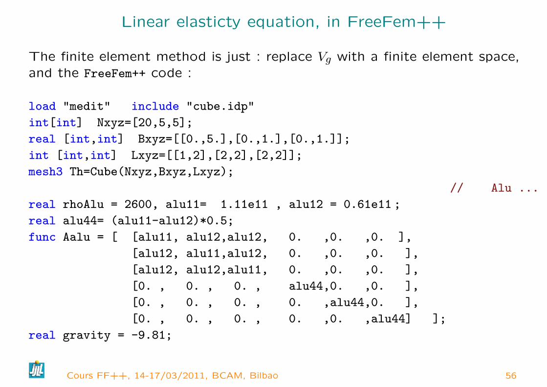
Linear elasticty equation, in FreeFem++
The finite element method is just : replace Vg with a finite element space,and the FreeFem++ code :
load "medit" include "cube.idp"
int[int] Nxyz=[20,5,5];
real [int,int] Bxyz=[[0.,5.],[0.,1.],[0.,1.]];
int [int,int] Lxyz=[[1,2],[2,2],[2,2]];
mesh3 Th=Cube(Nxyz,Bxyz,Lxyz);
// Alu ...
real rhoAlu = 2600, alu11= 1.11e11 , alu12 = 0.61e11 ;
real alu44= (alu11-alu12)*0.5;
func Aalu = [ [alu11, alu12,alu12, 0. ,0. ,0. ],
[alu12, alu11,alu12, 0. ,0. ,0. ],
[alu12, alu12,alu11, 0. ,0. ,0. ],
[0. , 0. , 0. , alu44,0. ,0. ],
[0. , 0. , 0. , 0. ,alu44,0. ],
[0. , 0. , 0. , 0. ,0. ,alu44] ];
real gravity = -9.81;
Cours FF++, 14-17/03/2011, BCAM, Bilbao 56

Linear elasticty equation, in FreeFem++
The problem code :
fespace Vh(Th,[P1,P1,P1]);
Vh [u1,u2,u3], [v1,v2,v3];
macro Strain(u1,u2,u3) [dx(u1),dy(u2),dz(u3),(dz(u2)+dy(u3)),
(dz(u1)+dx(u3)),(dy(u1)+dx(u2))] // EOM
macro div(u1,u2,u3) ( dx(u1)+dy(u2)+dz(u3) ) // EOM
solve Lame([u1,u2,u3],[v1,v2,v3])=
int3d(Th)( Strain(v1,v2,v3)’*(Aalu*Strain(u1,u2,u3)) )
- int3d(Th) ( rhoAlu*gravity*v3) + on(1,u1=0,u2=0,u3=0) ;
real coef= 0.1/u1[].linfty; int[int] ref2=[1,0,2,0];
mesh3
Thm=movemesh3(Th,transfo=[x+u1*coef,y+u2*coef,z+u3*coef],label=ref2);
plot(Th,Thm, wait=1,cmm="coef amplification = "+coef );
medit("Th-Thm",Th,Thm);
Cours FF++, 14-17/03/2011, BCAM, Bilbao 57
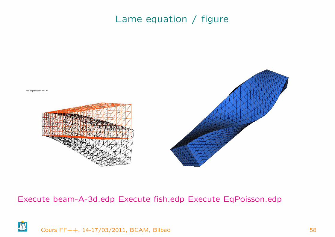
Lame equation / figure
Execute beam-A-3d.edp Execute fish.edp Execute EqPoisson.edp
Cours FF++, 14-17/03/2011, BCAM, Bilbao 58

Linear elasticty equation Eigen Value
The code to compute and show eigen vector of the Linear elasticty equation
varf vLame([u1,u2,u3],[v1,v2,v3])=int3d(Th)( Strain(v1,v2,v3)’*(Aalu*Strain(u1,u2,u3)) )+ on(1,u1=0,u2=0,u3=0) ;
varf vMass([u1,u2,u3],[v1,v2,v3])= int3d(Th)( [v1,v2,v3]’*[u1,u2,u3]*rhoalu );
matrix A= vLame(Vh,Vh,solver=sparsesolver);matrix B= vMass(Vh,Vh,solver=CG,eps=1e-20);
int nev=20; // number of computed eigen value close to 0real[int] ev(nev); // to store nev eigein valueVh[int] [eu1,eu2,eu3](nev); // to store nev eigen vectorint k=EigenValue(A,B,sym=true,value=ev,vector=eu1,tol=1e-10);
nev=min(k,nev); // some time the number of converged EV. can be greater than nev;for (int i=0;i<nev;i++) real coef= 0.5/eu1[i][].linfty;
mesh3 Thm=movemesh3(Th,transfo=[x+eu1[i]*coef,y+eu2[i]*coef,z+eu3[i]*coef]);medit("Thm-"+ev[i],Thm,wait=1);
Execute beam-EV-3d.edp
Cours FF++, 14-17/03/2011, BCAM, Bilbao 59
α periodic Finite element trick
Compute a Poisson problem in domain ]0, p[×]− 1,1[ with α-periodic
condition on vertical boundary Γp ( u(0, y) = αu(p, y) where α is a complex
number such that α = e2iπγ) and u is given on top and bottom border Γd.
Denote
Vα = u ∈ H1(Ω); u(0, y) = αu(p, y), V0α = u ∈ Vα;uΓd = 0
Find u ∈ Vα and u given on Γd such that
∀v ∈ V0α,∫
Ω∇u.∇v −
∫Γrv∂u
∂~n=∫
Ωfv, (6)
denote ϕα = e2iπγx/p we have u ∈ Vα iff ϕαu ∈ V1. So the problem is
equivalent to find uα = uϕα ∈ V1 uαϕα given on Γd such that
∀vα ∈ V01,∫
Ω∇αuα.∇αvα −
∫Γrvα∂uα
∂~n=∫
Ωfvαϕα, (7)
where ∇αu = ∇(ϕαu) = ϕα∇u+ uϕα∣∣∣ 2iπγ/p
0
Cours FF++, 14-17/03/2011, BCAM, Bilbao 60

Coupling periodic Finite element / BEM
Compute a Poisson problem in semi ∞ domain ]0, p[×]− 1,∞[ with periodic
condition on vertical boundary u(0, y) = u(p, y).
Let Γb the straight border of length p // to x axis, with normal equal to
~n =∣∣∣ 0
1 at y = 0 We need to add border term in the variational formulation∫Ω∇u.∇v −
∫Γbv∂u
∂~n=∫
Ωfv, ∀v.. (8)
The term contain the semi infinite modelization part.
Cours FF++, 14-17/03/2011, BCAM, Bilbao 61

Coupling periodic Finite element / BEM
We decompose wi the basis finite element function in the orthogonal de
Fourier basic on border Γb = x ∈ [0, p[, y = 0
fn = exp(−2π(inx+ |n|y)/p),∫
Γbfnfm = pδmn
. Remark −∆fn = 0, fn(x,+∞) = 0 , and we have
wi =∑n
cin fn and by orthogonality cim = 1/p∫
Γbwi fm
and ∂fn∂~n = −gnfn with gn = 2π|n|/p So we have :
−∫
Γbwidn(wj)ds = p
∑n
gn cin cjn
Cours FF++, 14-17/03/2011, BCAM, Bilbao 62

Trick to extract the degree of freedom on label 1 in know order
mesh Th=square(10,10);fespace Vh(Th,[P2,P2]); // exemple of finite elementint[int] ib(0:Vh.ndof-1); // arry ib[i]=i of size the number of DoF // for memory management: all locals are remove at end of block// to get numbering in good order ..// for u1: x-10 alway <0// for u2: x-10 + 1e-10 alway <0 but a little gearter than u1 so after// after sort we have u1 u2 node 1,u1 u2 node 1, .... with node numbering x // at the begin of the array
varf vbord([u1,u2],[v1,v2]) = on(1,u1=x-10,u2=x-10+1e-10);real[int] xb=vbord(0,Vh,tgv=1); // get the interpolation on border 1 .sort(xb,ib); // sort of 2 array in parallel// so now the begin of the array is the dof on label 1 and in ib we have the numberingxb = xb ? 1 : 0;int ndofon1 = xb.sum +0.5; // to count the number of non zero.ib.resize(ndofon1); // resize of the arraycout << ib << endl;
Execute BEM.edp
Cours FF++, 14-17/03/2011, BCAM, Bilbao 63

Schwaz algorithm
Let Ωi i ∈ I an overlaping of Ω, Let Pi a partition of the unite (∑Pi = 1 on
Ω) such that supp(Pi) ⊂ Ωi To solve :
−∆u = f in Ω, u = 0 on ∂Ω
the algorithm is just : let u0 a given solution, and n = 0
For all i ∈ I solve :
−∆un+1i = f in Ωi
un+1i = un on ∂Ωi ∩Ω
un+1i = 0 on ∂Ωi ∩ ∂Ω
n = n+ 1
un =∑i∈I
Piuni
To build the partition with metis, the overlapping is simply done with a loopn times of a successive L2 projection P0 7→ P1 7→ P0 to have n layeroverlapping.
Execute schwarz-nm.edp Execute schwarz-3.edp
Cours FF++, 14-17/03/2011, BCAM, Bilbao 64

Quelques exemples 3D
– Execute examples++-3d/beam-3d.edp
– Execute examples++-3d/3d-Leman.edp
– Execute examples++-3d/Lac.edp
– Execute examples++-3d/Laplace3d.edp
– Execute examples++-3d/LaplaceRT-3d.edp
– Execute examples++-3d/NSI3d.edp
– Execute examples++-3d/Period-Poisson-cube-ballon.edp
– Execute examples++-3d/Poisson-cube-ballon.edp
– Execute examples++-3d/Poisson3d.edp
– Execute examples++-3d/Stokes.edp
– Execute examples++-3d/convect-3d.edp
– Execute examples++-3d/cube-period.edp
Cours FF++, 14-17/03/2011, BCAM, Bilbao 65

Quelques exemples avec PLUGIN
– Execute examples++-load/metis.edp
– Execute examples++-load/LaplaceP4.edp
– Execute examples++-load/NSP2BRP0.edp
– Execute examples++-load/SuperLU.edp
– Execute examples++-load/bilapMorley.edp
– Execute examples++-load/buildlayermesh.edp
– Execute examples++-load/plot-fb-P4dc.edp
– Execute examples++-load/provadxw.edp
– Execute examples++-load/refinesphere.edp
– Execute examples++-load/tetgencube.edp
– Execute examples++-load/tetgenholeregion.edp
– Execute examples++-load/tetgenholeregion rugby.edp
Cours FF++, 14-17/03/2011, BCAM, Bilbao 66
Quelques examples 2D
– Execute BlackScholes2D.edp
– Execute cavityNewtow.edp
– Execute Poisson-mesh-adap.edp
– Execute Micro-wave.edp
– Execute wafer-heating-laser-axi.edp
– Execute nl-elast-neo-Hookean.edp
– Execute Stokes-eigen.edp
– Execute fluid-Struct-with-Adapt.edp
– Execute optim-control.edp
– Execute VI-2-menbrane-adap.edp
Cours FF++, 14-17/03/2011, BCAM, Bilbao 67
Exemple //
Execute examples++-mpi/schwarz-3.edp
Execute schwarz-nm.edp
Cours FF++, 14-17/03/2011, BCAM, Bilbao 68
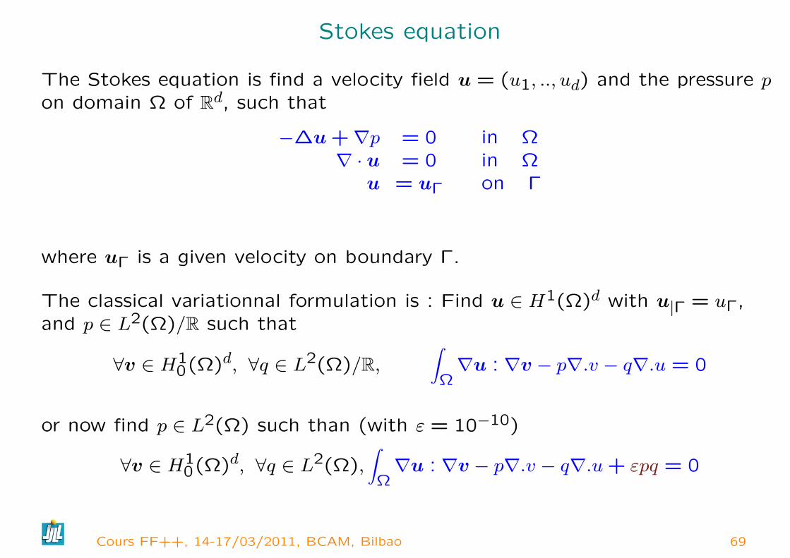
Stokes equation
The Stokes equation is find a velocity field u = (u1, .., ud) and the pressure pon domain Ω of Rd, such that
−∆u +∇p = 0 in Ω∇ · u = 0 in Ω
u = uΓ on Γ
where uΓ is a given velocity on boundary Γ.
The classical variationnal formulation is : Find u ∈ H1(Ω)d with u|Γ = uΓ,and p ∈ L2(Ω)/R such that
∀v ∈ H10(Ω)d, ∀q ∈ L2(Ω)/R,
∫Ω∇u : ∇v − p∇.v − q∇.u = 0
or now find p ∈ L2(Ω) such than (with ε = 10−10)
∀v ∈ H10(Ω)d, ∀q ∈ L2(Ω),
∫Ω∇u : ∇v − p∇.v − q∇.u+ εpq = 0
Cours FF++, 14-17/03/2011, BCAM, Bilbao 69

Stokes equation in FreeFem++
... build mesh .... Th (3d) T2d ( 2d)
fespace VVh(Th,[P2,P2,P2,P1]); // Taylor Hood Finite element.
macro Grad(u) [dx(u),dy(u),dz(u)] // EOM
macro div(u1,u2,u3) (dx(u1)+dy(u2)+dz(u3)) // EOM
varf vStokes([u1,u2,u3,p],[v1,v2,v3,q]) = int3d(Th)(
Grad(u1)’*Grad(v1) + Grad(u2)’*Grad(v2) + Grad(u3)’*Grad(v3)
- div(u1,u2,u3)*q - div(v1,v2,v3)*p + 1e-10*q*p )
+ on(1,u1=0,u2=0,u3=0) + on(2,u1=1,u2=0,u3=0);
matrix A=vStokes(VVh,VVh); set(A,solver=UMFPACK);
real[int] b= vStokes(0,VVh);
VVh [u1,u2,u3,p]; u1[]= A^-1 * b;
// 2d intersection of plot
fespace V2d(T2d,P2); // 2d finite element space ..
V2d ux= u1(x,0.5,y); V2d uz= u3(x,0.5,y); V2d p2= p(x,0.5,y);
plot([ux,uz],p2,cmm=" cut y = 0.5");
Execute Stokes3d.edp
Cours FF++, 14-17/03/2011, BCAM, Bilbao 70

Stokes equation with Stabilization term / T. Chacon
If you use Finite element P2 in velocity and pressure, then we need a
stabilization term. The term to be add to the classical variational
formulation is :
D = −∑
K∈Th
∫KτKRh(∂xp)Rh(∂xq) + Rh(∂yp) (Rh∂yq)dx
with
Rh = Id− IhPhand where
Vh P1 continuous finite space
V dch P1 fully discontinuous finite space
Ih the trivial injection form Vh to V dch
Ph an interpolation operator form V dch to Vh
Id the identity V dch 7→ V dch .
Cours FF++, 14-17/03/2011, BCAM, Bilbao 71

How to build Rh in FreeFem++
matrix Ih = interpolate(Vdch,Vh);
matrix Ph = interpolate(Vh,Vdch);
if(!scootzhang)
// Clement’s Operator or L2 projection with mass lumping
varf vsigma(u,v)=int2d(Th)(v);
Vh sigma; sigma[]=vsigma(0,Vh); // σi =∫Ωwi
varf vP2L(u,v)=int2d(Th,qft=qf1pTlump)(u*v/sigma); // P1 Mass Lump
Ph=vP2L(Vdch,Vh);
matrix IPh = Ih*Ph ;
real[int] un(IPh.n); un=1;
matrix Id=un;
Rh = Id + (-1.)*IPh; // Id−Rhh
Cours FF++, 14-17/03/2011, BCAM, Bilbao 72

How to build the D matrix in FreeFem++
....fespace Wh(Th,[P2,P2,P2]); // the Stokes FE Spacefespace Vh(Th,P1); fespace Vdch(Th,P1dc);....matrix D; // the variable to store the matrix D varf vMtk(p,q)=int2d(Th)(hTriangle*hTriangle*ctk*p*q);matrix Mtk=vMtk(Vdch,Vdch);int[int] c2=[2]; // take the 2 second component of Wh.matrix Dx = interpolate(Vdch,Wh,U2Vc=c2,op=1); // ∂xp discrete operatormatrix Dy = interpolate(Vdch,Wh,U2Vc=c2,op=2); // ∂yp discrete operatormatrix Rh;
... add Build of Rh code hereDx = Rh*Dx; Dy = Rh*Dy;
// Sorry matrix operation is done one by one.matrix DDxx= Mtk*Dx; DDxx = Dx’*DDxx;matrix DDyy= Mtk*Dy; DDyy = Dy’*DDyy;D = DDxx + DDyy;
// cleaning all local matrix and array.A = A + D; // add to the Stokes matrix....
Execute Stokes-tomas.edp
Cours FF++, 14-17/03/2011, BCAM, Bilbao 73
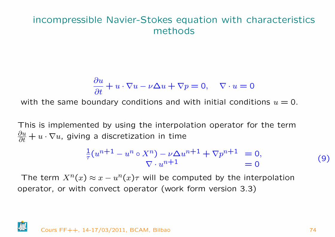
incompressible Navier-Stokes equation with characteristicsmethods
∂u
∂t+ u · ∇u− ν∆u+∇p = 0, ∇ · u = 0
with the same boundary conditions and with initial conditions u = 0.
This is implemented by using the interpolation operator for the term∂u∂t + u · ∇u, giving a discretization in time
1τ (un+1 − un Xn)− ν∆un+1 +∇pn+1 = 0,
∇ · un+1 = 0(9)
The term Xn(x) ≈ x− un(x)τ will be computed by the interpolation
operator, or with convect operator (work form version 3.3)
Cours FF++, 14-17/03/2011, BCAM, Bilbao 74
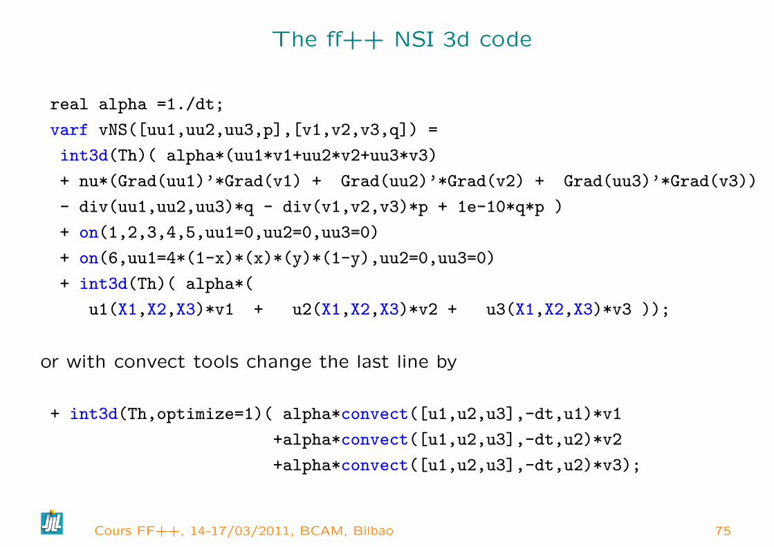
The ff++ NSI 3d code
real alpha =1./dt;
varf vNS([uu1,uu2,uu3,p],[v1,v2,v3,q]) =
int3d(Th)( alpha*(uu1*v1+uu2*v2+uu3*v3)
+ nu*(Grad(uu1)’*Grad(v1) + Grad(uu2)’*Grad(v2) + Grad(uu3)’*Grad(v3))
- div(uu1,uu2,uu3)*q - div(v1,v2,v3)*p + 1e-10*q*p )
+ on(1,2,3,4,5,uu1=0,uu2=0,uu3=0)
+ on(6,uu1=4*(1-x)*(x)*(y)*(1-y),uu2=0,uu3=0)
+ int3d(Th)( alpha*(
u1(X1,X2,X3)*v1 + u2(X1,X2,X3)*v2 + u3(X1,X2,X3)*v3 ));
or with convect tools change the last line by
+ int3d(Th,optimize=1)( alpha*convect([u1,u2,u3],-dt,u1)*v1
+alpha*convect([u1,u2,u3],-dt,u2)*v2
+alpha*convect([u1,u2,u3],-dt,u2)*v3);
Cours FF++, 14-17/03/2011, BCAM, Bilbao 75
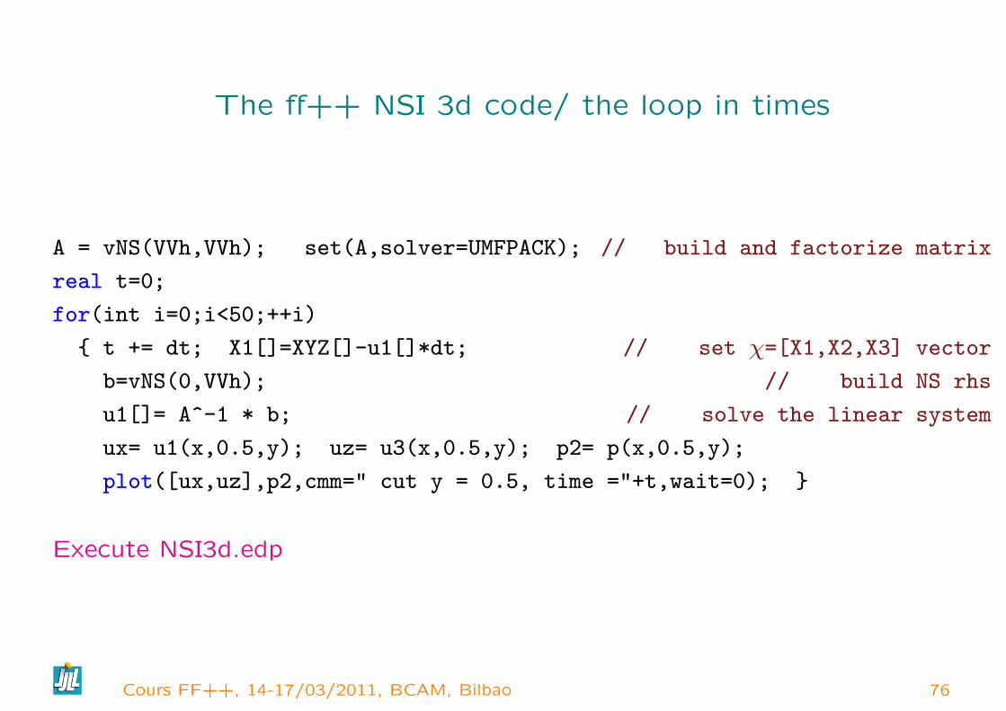
The ff++ NSI 3d code/ the loop in times
A = vNS(VVh,VVh); set(A,solver=UMFPACK); // build and factorize matrix
real t=0;
for(int i=0;i<50;++i)
t += dt; X1[]=XYZ[]-u1[]*dt; // set χ=[X1,X2,X3] vector
b=vNS(0,VVh); // build NS rhs
u1[]= A^-1 * b; // solve the linear system
ux= u1(x,0.5,y); uz= u3(x,0.5,y); p2= p(x,0.5,y);
plot([ux,uz],p2,cmm=" cut y = 0.5, time ="+t,wait=0);
Execute NSI3d.edp
Cours FF++, 14-17/03/2011, BCAM, Bilbao 76

Dynamics Load facility
Or How to add your C++ function in FreeFem++.
First, like in cooking, the first true difficulty is how to use the kitchen.
I suppose you can compile the first example for the examples++-load
numermac11:FH-Seville hecht# ff-c++ myppm2rnm.cppexport MACOSX_DEPLOYMENT_TARGET=10.3g++ -c -DNDEBUG -O3 -O3 -march=pentium4 -DDRAWING -DBAMG_LONG_LONG -DNCHECKPTR-I/usr/X11/include -I/usr/local/lib/ff++/3.4/include ’myppm2rnm.cpp’g++ -bundle -undefined dynamic_lookup -DNDEBUG -O3 -O3 -march=pentium4 -DDRAWING-DBAMG_LONG_LONG -DNCHECKPTR -I/usr/X11/include ’myppm2rnm.o’ -o myppm2rnm.dylib
add tools to read pgm image
Cours FF++, 14-17/03/2011, BCAM, Bilbao 77
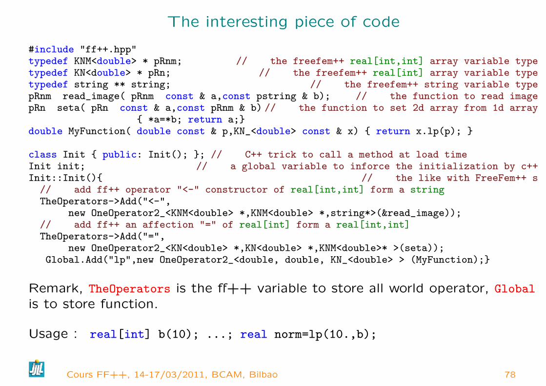
The interesting piece of code
#include "ff++.hpp"typedef KNM<double> * pRnm; // the freefem++ real[int,int] array variable typetypedef KN<double> * pRn; // the freefem++ real[int] array variable typetypedef string ** string; // the freefem++ string variable typepRnm read_image( pRnm const & a,const pstring & b); // the function to read imagepRn seta( pRn const & a,const pRnm & b) // the function to set 2d array from 1d array
*a=*b; return a;double MyFunction( double const & p,KN_<double> const & x) return x.lp(p);
class Init public: Init(); ; // C++ trick to call a method at load timeInit init; // a global variable to inforce the initialization by c++Init::Init() // the like with FreeFem++ s// add ff++ operator "<-" constructor of real[int,int] form a stringTheOperators->Add("<-",
new OneOperator2_<KNM<double> *,KNM<double> *,string*>(&read_image));// add ff++ an affection "=" of real[int] form a real[int,int]TheOperators->Add("=",
new OneOperator2_<KN<double> *,KN<double> *,KNM<double>* >(seta));Global.Add("lp",new OneOperator2_<double, double, KN_<double> > (MyFunction);
Remark, TheOperators is the ff++ variable to store all world operator, Global
is to store function.
Usage : real[int] b(10); ...; real norm=lp(10.,b);
Cours FF++, 14-17/03/2011, BCAM, Bilbao 78

The prototype
OneOperator2_<returntype ,typearg1 ,typearg2>(& thefunction ));
returntype thefunction(typearg1 const &, typearg2 const &)
To get the C++ type of all freefem++ type, method, operator : just do in
examples++-tutorial directory
c++filt -t < lestablesCmatrix 293 Matrice_Creuse<std::complex<double> >R3 293 Fem2D::R3bool 293 bool*complex 293 std::complex<double>*func 294 C_F0ifstream 293 std::basic_istream<char, std::char_traits<char> >**int 293 long*matrix 293 Matrice_Creuse<double>mesh 293 Fem2D::Mesh**mesh3 293 Fem2D::Mesh3**ofstream 293 std::basic_ostream<char, std::char_traits<char> >**problem 294 Problemreal 293 double*string 293 std::basic_string<char, std::char_traits<char>, std::allocator<char> >**
Cours FF++, 14-17/03/2011, BCAM, Bilbao 79
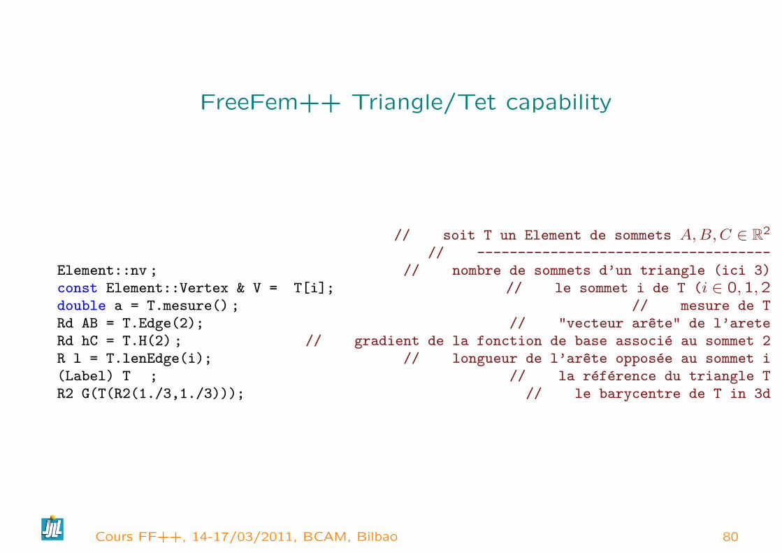
FreeFem++ Triangle/Tet capability
// soit T un Element de sommets A,B,C ∈ R2
// ------------------------------------Element::nv ; // nombre de sommets d’un triangle (ici 3)const Element::Vertex & V = T[i]; // le sommet i de T (i ∈ 0,1,2double a = T.mesure() ; // mesure de TRd AB = T.Edge(2); // "vecteur arete" de l’areteRd hC = T.H(2) ; // gradient de la fonction de base associe au sommet 2R l = T.lenEdge(i); // longueur de l’arete opposee au sommet i(Label) T ; // la reference du triangle TR2 G(T(R2(1./3,1./3))); // le barycentre de T in 3d
Cours FF++, 14-17/03/2011, BCAM, Bilbao 80
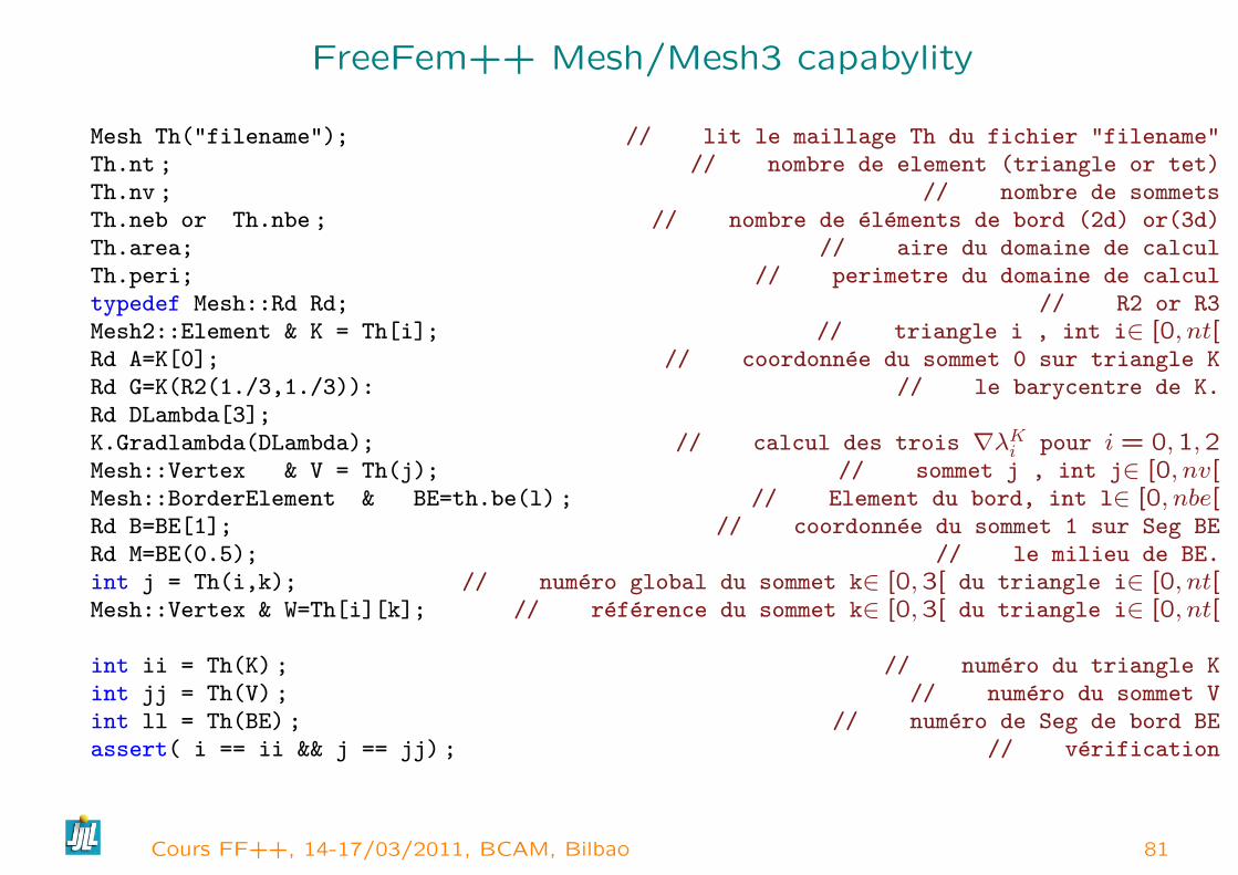
FreeFem++ Mesh/Mesh3 capabylity
Mesh Th("filename"); // lit le maillage Th du fichier "filename"Th.nt ; // nombre de element (triangle or tet)Th.nv ; // nombre de sommetsTh.neb or Th.nbe ; // nombre de elements de bord (2d) or(3d)Th.area; // aire du domaine de calculTh.peri; // perimetre du domaine de calcultypedef Mesh::Rd Rd; // R2 or R3Mesh2::Element & K = Th[i]; // triangle i , int i∈ [0, nt[Rd A=K[0]; // coordonnee du sommet 0 sur triangle KRd G=K(R2(1./3,1./3)): // le barycentre de K.Rd DLambda[3];K.Gradlambda(DLambda); // calcul des trois ∇λKi pour i = 0,1,2Mesh::Vertex & V = Th(j); // sommet j , int j∈ [0, nv[Mesh::BorderElement & BE=th.be(l) ; // Element du bord, int l∈ [0, nbe[Rd B=BE[1]; // coordonnee du sommet 1 sur Seg BERd M=BE(0.5); // le milieu de BE.int j = Th(i,k); // numero global du sommet k∈ [0,3[ du triangle i∈ [0, nt[Mesh::Vertex & W=Th[i][k]; // reference du sommet k∈ [0,3[ du triangle i∈ [0, nt[
int ii = Th(K) ; // numero du triangle Kint jj = Th(V) ; // numero du sommet Vint ll = Th(BE) ; // numero de Seg de bord BEassert( i == ii && j == jj) ; // verification
Cours FF++, 14-17/03/2011, BCAM, Bilbao 81
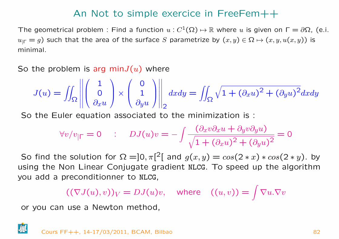
An Not to simple exercice in FreeFem++
The geometrical problem : Find a function u : C1(Ω) 7→ R where u is given on Γ = ∂Ω, (e.i.
u|Γ = g) such that the area of the surface S parametrize by (x, y) ∈ Ω 7→ (x, y, u(x, y)) is
minimal.
So the problem is arg minJ(u) where
J(u) =∫∫
Ω
∣∣∣∣∣∣∣∣∣∣∣∣∣∣ 1
0∂xu
× 0
1∂yu
∣∣∣∣∣∣∣∣∣∣∣∣∣∣2
dxdy =∫∫
Ω
√1 + (∂xu)2 + (∂yu)2dxdy
So the Euler equation associated to the minimization is :
∀v/v|Γ = 0 : DJ(u)v = −∫ (∂xv∂xu+ ∂yv∂yu)√
1 + (∂xu)2 + (∂yu)2= 0
So find the solution for Ω =]0, π[2[ and g(x, y) = cos(2 ∗ x) ∗ cos(2 ∗ y). byusing the Non Linear Conjugate gradient NLCG. To speed up the algorithmyou add a preconditionner to NLCG,
((∇J(u), v))V = DJ(u)v, where ((u, v)) =∫∇u.∇v
or you can use a Newton method,
Cours FF++, 14-17/03/2011, BCAM, Bilbao 82
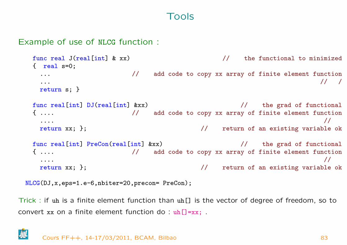
Tools
Example of use of NLCG function :
func real J(real[int] & xx) // the functional to minimized real s=0;... // add code to copy xx array of finite element function... // /return s;
func real[int] DJ(real[int] &xx) // the grad of functional .... // add code to copy xx array of finite element function.... //return xx; ; // return of an existing variable ok
func real[int] PreCon(real[int] &xx) // the grad of functional .... // add code to copy xx array of finite element function.... //return xx; ; // return of an existing variable ok
NLCG(DJ,x,eps=1.e-6,nbiter=20,precon= PreCon);
Trick : if uh is a finite element function than uh[] is the vector of degree of freedom, so to
convert xx on a finite element function do : uh[]=xx; .
Cours FF++, 14-17/03/2011, BCAM, Bilbao 83
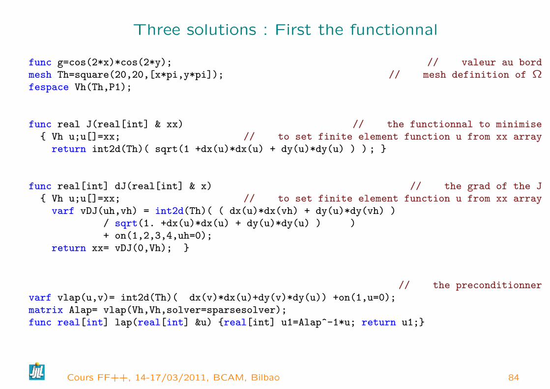
Three solutions : First the functionnal
func g=cos(2*x)*cos(2*y); // valeur au bordmesh Th=square(20,20,[x*pi,y*pi]); // mesh definition of Ωfespace Vh(Th,P1);
func real J(real[int] & xx) // the functionnal to minimise Vh u;u[]=xx; // to set finite element function u from xx arrayreturn int2d(Th)( sqrt(1 +dx(u)*dx(u) + dy(u)*dy(u) ) ) ;
func real[int] dJ(real[int] & x) // the grad of the J Vh u;u[]=xx; // to set finite element function u from xx arrayvarf vDJ(uh,vh) = int2d(Th)( ( dx(u)*dx(vh) + dy(u)*dy(vh) )
/ sqrt(1. +dx(u)*dx(u) + dy(u)*dy(u) ) )+ on(1,2,3,4,uh=0);
return xx= vDJ(0,Vh);
// the preconditionnervarf vlap(u,v)= int2d(Th)( dx(v)*dx(u)+dy(v)*dy(u)) +on(1,u=0);matrix Alap= vlap(Vh,Vh,solver=sparsesolver);func real[int] lap(real[int] &u) real[int] u1=Alap^-1*u; return u1;
Cours FF++, 14-17/03/2011, BCAM, Bilbao 84
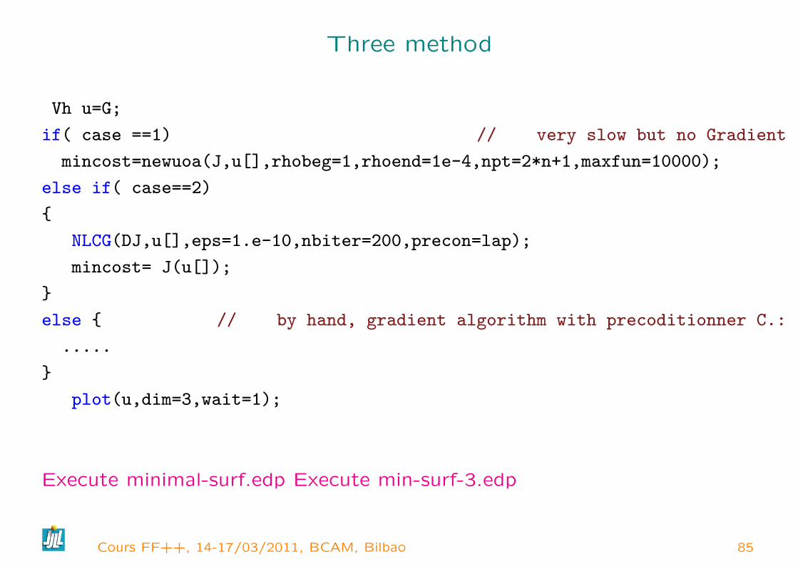
Three method
Vh u=G;
if( case ==1) // very slow but no Gradient
mincost=newuoa(J,u[],rhobeg=1,rhoend=1e-4,npt=2*n+1,maxfun=10000);
else if( case==2)
NLCG(DJ,u[],eps=1.e-10,nbiter=200,precon=lap);
mincost= J(u[]);
else // by hand, gradient algorithm with precoditionner C.:
.....
plot(u,dim=3,wait=1);
Execute minimal-surf.edp Execute min-surf-3.edp
Cours FF++, 14-17/03/2011, BCAM, Bilbao 85
Conclusion and Future
It is a useful tool to teaches Finite Element Method, and to test some
nontrivial algorithm.
– Optimization FreeFem++ in 3d
– All graphic with OpenGL (in construction)
– Galerkin discontinue (do in 2d, to do in 3d)
– 3D ( under construction )
– automatic differentiation ( under construction )
– // linear solver and build matrix //
– 3d mesh adaptation
– Suite et FIN. (L’avenir ne manque pas de future et lycee de Versailles)
Thank, for your attention ?
Cours FF++, 14-17/03/2011, BCAM, Bilbao 86