1

Freight Movement Model Development for Oklahoma

PHASE I V RE PORT: COMBINED REGIONAL-STAT E FREIGHT MOVEMENT

MODEL AND FLIPS SOFT WAR E PROTOT YPE

Developed and Presented by:

Oklahoma State University

University of Oklahoma

Faculty Members

Ricki G. Ingalls, Ph.D. Associate Professor in School of Industrial

Engineering and Management

Manjunath Kamath, Ph.D. Professor and Graduate Coordinator in School

of Industrial Engineering and Management

Graduate Research Assistants

Kedar Adavadkar Karthik Ayodhiramanujan

Harsha Dhavala Rengarajan Parthasarathi

Peerapol Sittivijan Sandeep Srivathsan

Faculty Members

Guoqiang Shen, Ph.D. Associate Professor and Director in Division of

Regional and City Planning

P. Simin Pulat, Ph.D. Professor and Associate Dean in School of

Industrial Engineering

Graduate Research Assistants

Gizem Aydin Justin Lebeau Charu Ojha Jiahui Wang

This material is based upon work partially supported by the National Science Foundation under Grant No. IIP‐0732516.  Any opinions, findings, and conclusions or recommendations expressed in this material are those of the authors and do not necessarily reflect the views of the National Science Foundation. 

2

EXECUTIVE SUMMARY  The problem of forecasting freight movement into the future is a complex combination of data management, demand and supply forecasting, and modeling the distribution of freight flow. In addition, the difficult task of developing software is necessary to support each of these areas. Each of these areas taken by itself is a difficult research area. However, over the last 6 years, the Freight Movement Model for the State of Oklahoma (FMM) project has tackled each of these problems and has successfully developed a software prototype that addresses data management, forecasting, and modeling the distribution of freight flow. This project was one of the original Oklahoma Transportation Center (OTC) projects in 2003. Through several funding cycles over the past six years, the OTC, with funding from the Oklahoma Department of Transportation and the United States Department of Transportation, has invested in this research. The results of this research include methodology and prototype software that can model freight flow on all major highways, waterways, and railways in the United States at the state or Metropolitan Statistical Area (MSA) level and in Oklahoma at the county level. Two major contributions of this research are the ability to forecast the effect of changing freight demands into the future and the ability to model the effect of infrastructure changes such as interstate highway expansions and/or closing. As this project closes, the research team is confident that this work can be used in a variety of applications including infrastructure planning and disaster recovery planning. There are two primary problems addressed by this research. First, this project has developed a methodology that models freight movement within, into, out of, and through the state. It models freight movement not only on highways, but also on railway and waterway networks in the nation and the state. Second, this project has developed a methodology that takes public database information, systematically cleanses that data, and uses the data in the forecasting of freight flows. Solutions to these two problems are part of a prototype software system that can be used to analyze freight flows by commodity and by mode in a given future year. The research team was led by Drs. Ricki Ingalls and Manjunath Kamath of Oklahoma State University and Drs. Simin Pulat and Guoqiang Shen of The University of Oklahoma. The FMM project has been an excellent example of collaboration between the two universities and has funded many graduate research assistants over the life of the project. The Freight Movement Model is an asset for Oklahoma in planning and executing projects related to improving freight movement in the state. The growth of the Oklahoma economy will continue to rely on the efficient movement of freight in the state and the Freight Movement Model can be a vital part in planning that future.

3

List of Contents 

1.  INTRODUCTION ............................................................................................................................................. 9 

1.1 PROBLEM STATEMENT AND RESEARCH ACCOMPLISHMENTS ............................................................................................. 9 1.2 SUPPORT OF OKLAHOMA’S LONG‐RANGE TRANSPORTATION PLANNING AND POLICY .......................................................... 11 1.3 RESEARCH OUTCOMES ............................................................................................................................................ 11 1.4 OUTLINE OF THE REPORT ......................................................................................................................................... 12 

2.  FREIGHT MOVEMENT MODELING METHODOLOGY ....................................................................................... 13 

2.1 FMM METHODOLOGY............................................................................................................................................ 13 2.1.1 Freight Generation .................................................................................................................................... 15 

2.1.1.1 Freight Production .............................................................................................................................................. 15 2.1.1.2 Freight Attraction ................................................................................................................................................ 16 

2.1.2 Freight Distribution ................................................................................................................................... 16 2.1.2.1  Doubly Constrained Growth Factor Methods to Calibrate Tijn ................................................................... 16 2.1.2.2  Doubly Constrained Gravity Model to Calibrate Tijn ................................................................................... 17 

2.1.3 Freight Modal Split Model ......................................................................................................................... 18 2.1.4 Freight Flow Assignment Model ................................................................................................................ 18 

2.1.4.1  All–or–Nothing Assignment ....................................................................................................................... 19 2.1.4.2  System Optimal Assignment ...................................................................................................................... 20 2.1.4.3  User Equilibrium Assignment ..................................................................................................................... 20 2.1.4.4  Stochastic User Equilibrium Assignment .................................................................................................... 20 

2.2 TIMELINE OF THE FREIGHT MOVEMENT MODELING PROJECT .......................................................................................... 21 

3.  IDENTIFICATION OF DATA SOURCES AND ISSUES WITH AVAILABILITY AND PREPARATION OF DATA .............. 22 

3.1 IDENTIFICATION OF DATA SOURCES ........................................................................................................................... 22 3.1.1 Classification of Data Sources ................................................................................................................... 22 

3.1.1.1 Commodity Flow Databases ................................................................................................................................ 22 3.1.1.2 Auxiliary Databases ............................................................................................................................................. 22 3.1.1.3 Network Databases ............................................................................................................................................. 23 

3.2 ISSUES WITH DATA AVAILABILITY AND PREPARATION OF INPUT DATA ............................................................................... 23 3.2.1 The Base Year Selection ............................................................................................................................. 23 3.2.2 Developing Commodity Groups ................................................................................................................. 23 3.2.3 Relating Commodity Groups to Industrial Sectors or Economic Indicators ............................................... 24 3.2.4 Finding the Commodity Flows ................................................................................................................... 27 3.2.5 Finding the Socio‐Economic Variables ....................................................................................................... 27 3.2.6 Finding the Network Information .............................................................................................................. 27 

4.  COMBINED REGIONAL‐STATE MODEL ........................................................................................................... 28 

4.1 SIGNIFICANCE OF THE COMBINED REGIONAL‐STATE MODEL ........................................................................................... 28 4.2 PREPARATION OF NETWORK DATA FOR FLOW ASSIGNMENT ........................................................................................... 29 

4.2.1 Highway Network ...................................................................................................................................... 29 4.2.2 Railway Network ....................................................................................................................................... 32 4.2.3 Waterway Network ................................................................................................................................... 33 

4.3 PREPARATION OF FREIGHT DATA ............................................................................................................................... 34 4.3.1 Code Mapping ........................................................................................................................................... 35 4.3.2 State to County Split for Oklahoma ........................................................................................................... 35 4.3.3 Tonnage to Truck Conversion .................................................................................................................... 38 4.3.4 Aggregation of Freight Flow for all Commodity Types .............................................................................. 39 

4.4 PREPARATION OF FREIGHT DATA FOR ASSIGNMENT USING TRANSCADTM ....................................................................... 39 4.4.1 Building of Origin‐Destination Matrix ....................................................................................................... 39 

4

4.4.2 Configuring the Network ........................................................................................................................... 39 4.5 CONDUCTING FLOW ASSIGNMENT USING TRANSCADTM .............................................................................................. 40 4.6 ANALYZING THE FLOW ASSIGNMENT RESULTS .............................................................................................................. 40 

4.6.1 Volume/Capacity Ratio .......................................................................................................................................... 40 4.6.2 Identifying Flow by Different Flow Types (From, To, Through, and Within) .......................................................... 40 

5.  RESULTS OF FREIGHT FLOW ASSIGNMENT .................................................................................................... 43 

5.1 MODEL VALIDATION ............................................................................................................................................... 43 5.2 PREDICTIONS FOR FUTURE YEAR (2015) .................................................................................................................... 44 

5.2.1 Total Flow on each Network ..................................................................................................................... 44 5.2.2 Volume/Capacity Ratio ............................................................................................................................. 48 5.2.3 Flow by Different Flow Types (From, To, Through, and Within) ................................................................ 50 5.2.4 Top Commodities for Oklahoma................................................................................................................ 54 5.2.5 Top Trading Partners for Oklahoma .......................................................................................................... 56 

6.  FMM PROTOTYPE SOFTWARE: FREIGHT LOGISTICS INFRASTRUCTURE PLANNING SYSTEM (FLIPS) ................. 59 

6.1 COMPONENTS OF THE FLIPS SOFTWARE .................................................................................................................... 59 6.1.1 FMM Pre‐Processor ................................................................................................................................... 59 6.1.2 FMM Main‐Processor ................................................................................................................................ 61 6.1.3 FMM Database .......................................................................................................................................... 61 6.1.4 FMM Geographic Database ...................................................................................................................... 61 6.1.5 FMM Visualization .................................................................................................................................... 61 

6.1.5.1 Summary of Freight Flow Analysis ...................................................................................................................... 62 6.1.5.2 Basic Queries ....................................................................................................................................................... 67 6.1.5.3 Advanced Queries ............................................................................................................................................... 71 

7.  SCENARIO ANALYSIS ..................................................................................................................................... 72 

7.1 BRIDGE COLLAPSE SCENARIO .................................................................................................................................... 72 7.1.1 Results from All‐or‐Nothing (AON) Assignment ........................................................................................ 72 

7.1.1.1 Pre‐Disaster and Post‐Disaster Assignment Comparison .................................................................................... 74 7.1.2 Results from User Equilibrium (UE) Assignment ........................................................................................ 77 

7.1.2.1 Pre‐Disaster and Post‐Disaster Assignment Comparison .................................................................................... 79 7.2 EMPLOYMENT AND POPULATION INCREASE SCENARIO ................................................................................................... 83 

7.2.1 Methodology ............................................................................................................................................. 83 7.2.2 Results and Analysis Under All‐or‐Nothing (AON) Assignment ................................................................. 88 7.2.3 Results and Analysis Under User Equilibrium (UE) Assignment ................................................................ 89 

8.  FUTURE RESEARCH ....................................................................................................................................... 91 

REFERENCES ...................................................................................................................................................... 92 

APPENDIX A: DATA SOURCES AND INPUT PARAMETERS .................................................................................... 94 

APPENDIX B: REGIONAL FREIGHT MOVEMENT MODEL ...................................................................................... 99 

B.1 FREIGHT GENERATION ............................................................................................................................................ 99 B.1.1 Freight Production ..................................................................................................................................... 99 

B.1.1.1 Freight Production – Mathematical Model ......................................................................................................... 99 B.1.1.2 Survey of Databases .......................................................................................................................................... 101 B.1.1.3 Regression Methodology .................................................................................................................................. 103 B.1.1.4 Results of Freight Production ............................................................................................................................ 106 

B.1.2 Freight Attraction .................................................................................................................................... 106 B.2 FREIGHT DISTRIBUTION USING A DOUBLY CONSTRAINED GRAVITY MODEL ...................................................................... 111 

B.2.1 Databases Required for the Gravity Model ............................................................................................. 111 B.2.2 Sample Results for Freight Distribution ................................................................................................... 112 

B.3 MODE‐SPLIT ....................................................................................................................................................... 112 

5

B.4 FREIGHT ASSIGNMENT .......................................................................................................................................... 113 

APPENDIX C: COMBINED REGIONAL–STATE MODEL ......................................................................................... 114 

C.1 INPUTS TO THE COMBINED REGIONAL‐STATE MODEL .................................................................................................. 114 C.1.1 Centroids for the Combined Regional‐State Model ................................................................................. 114 C.1.2 Payload Factors for Tonnage to Number of Trucks Conversion .............................................................. 119 

C.2 FLOW ASSIGNMENT RESULTS FOR BASE YEAR (2002) ................................................................................................. 120 C.2.1 Total flow on each network ..................................................................................................................... 120 C.2.2 Volume/Capacity Ratio ........................................................................................................................... 125 C.2.3 Flow by flow type .................................................................................................................................... 126 C.2.4 Top Commodities for Oklahoma ............................................................................................................. 128 C.2.5 Top Trading Partners for Oklahoma ........................................................................................................ 130 

APPENDIX D:  CAPACITATED NETWORK FREIGHT ASSIGNMENT USING SIMPLIFIED PIECEWISE LINEAR TRAVEL‐TIME FUNCTION .............................................................................................................................................. 133 

D.1 TRAVEL‐TIME FLOW CURVES ................................................................................................................................. 133 D.2 FORMULATION OF THE FREIGHT FLOW ASSIGNMENT PROBLEM .................................................................................... 135 

D.2.1 Model Nomenclature .............................................................................................................................. 135 D.2.1.1 Model Parameters ............................................................................................................................................ 135 D.2.1.2 Model Decision variables .................................................................................................................................. 135 

D.2.2 Model Objective and Constraints ............................................................................................................ 135 D.2.2.1 Objective Function ............................................................................................................................................ 135 D.2.2.2 Flow Balance Constraints for each OD pair k .................................................................................................... 136 D.2.2.3 Free Flow Threshold Constraints ...................................................................................................................... 136 D.2.2.4 Binary Variable Constraints .............................................................................................................................. 136 D.2.2.5 Non‐Negativity Constraints .............................................................................................................................. 136 

D.2.3 Model Formulation ................................................................................................................................. 137 D.3 MODEL VALIDATION ............................................................................................................................................ 137 D.4 MODEL ISSUES .................................................................................................................................................... 139 

APPENDIX E: USER’S MANUAL FOR FREIGHT LOGISTICS INFRASTRUCTURE PLANNING SOFTWARE (FLIPS) ........ 140 

E.1 INSTALLATION INSTRUCTIONS ................................................................................................................................. 140 E.2 GETTING STARTED ................................................................................................................................................ 141 E.3 FILE MENU ......................................................................................................................................................... 141 E.4 APPLICATIONS MENU ............................................................................................................................................ 141 

E.4.1 Freight Flow Summaries .......................................................................................................................... 142 E.4.1.1 Results: .............................................................................................................................................................. 142 

E.4.2 Basic Queries ........................................................................................................................................... 143 E.4.3 GIS Application Advanced Queries .......................................................................................................... 146 

6

List of Figures 

FIGURE 2.1: FREIGHT MOVEMENT MODELING METHODOLOGY ................................................................................................ 14 FIGURE 2.2: FREIGHT MOVEMENT MODELING PROJECT TIMELINE ............................................................................................. 21 FIGURE 3.1: CLASSIFICATION OF DATA SOURCES .................................................................................................................... 22 FIGURE 3.2 CODE MAPPING (ALGORITHM) ............................................................................................................................ 25 FIGURE 3.3: NAICS TO SCTG CODE MAPPING PROCEDURE ..................................................................................................... 26 FIGURE 4.1: FAF2 REGIONS ................................................................................................................................................ 28 FIGURE 4.2: FAF2 REGIONS WITH 77 COUNTIES IN OKLAHOMA ................................................................................................. 29 FIGURE 4.3: US HIGHWAY NETWORK – CONTINENTAL US ....................................................................................................... 31 FIGURE 4.4: US HIGHWAY NETWORK – ALASKA AND HAWAII ................................................................................................... 32 FIGURE 4.5: US RAILWAY NETWORK ................................................................................................................................... 32 FIGURE 4.6: US WATERWAY NETWORK ............................................................................................................................... 33 FIGURE 4.7: US WATERWAY NETWORK – ALASKA AND HAWAII ................................................................................................ 33 FIGURE 4.8: PREPARATION OF NETWORK DATA ..................................................................................................................... 34 FIGURE 4.9: CODE MAPPING SCHEME .................................................................................................................................. 35 FIGURE 4.10: COMBINED REGIONAL‐STATE MODEL ALGORITHM FOR THE HIGHWAY NETWORK (CAPACITATED FREIGHT FLOW 

ASSIGNMENT) ........................................................................................................................................................ 42 FIGURE 5.1: RANDOM LINKS IN TULSA REGION ...................................................................................................................... 43 FIGURE 5.2: COMPARISON OF THE FREIGHT ASSIGNMENT RESULTS WITH INCOG DATA ................................................................ 44 FIGURE 5.3: TOTAL FLOW ON HIGHWAY NETWORK IN 2015 BY ALL‐OR‐NOTHING ASSIGNMENT .................................................... 45 FIGURE 5.4: TOTAL FLOW ON HIGHWAY NETWORK IN 2015 BY SYSTEM OPTIMAL ASSIGNMENT ..................................................... 45 FIGURE 5.5: TOTAL FLOW ON HIGHWAY NETWORK IN 2015 BY USER EQUILIBRIUM ASSIGNMENT .................................................. 46 FIGURE 5.6: TOTAL FLOW ON HIGHWAY NETWORK IN 2015 BY STOCHASTIC USER EQUILIBRIUM ASSIGNMENT ................................. 46 FIGURE 5.7: TOTAL FLOW ON RAILWAY NETWORK IN 2015 IN U.S. .......................................................................................... 47 FIGURE 5.8: TOTAL FLOW ON RAILWAY NETWORK IN 2015 IN OKLAHOMA ................................................................................. 47 FIGURE 5.9: TOTAL FLOW ON WATERWAY NETWORK IN 2015 IN U.S. ...................................................................................... 48 FIGURE 5.10: TOTAL FLOW ON WATERWAY NETWORK IN 2015 IN OKLAHOMA ........................................................................... 48 FIGURE 5.11: V/C RATIO FOR HIGHWAY NETWORK IN 2015 BASED ON SYSTEM OPTIMAL ASSIGNMENT .......................................... 49 FIGURE 5.12: V/C RATIO FOR HIGHWAY NETWORK IN 2015 BASED ON USER EQUILIBRIUM ASSIGNMENT ........................................ 49 FIGURE 5.13: V/C RATIO FOR HIGHWAY NETWORK IN 2015 BASED ON STOCHASTIC USER EQUILIBRIUM ASSIGNMENT....................... 50 FIGURE 5.14: FLOW MAP FOR FROM‐FLOW ON THE US HIGHWAY NETWORK IN 2015................................................................. 50 FIGURE 5.15: A CLOSE‐UP VIEW OF 2015 FREIGHT FLOW FROM OKLAHOMA TO OTHER STATES .................................................... 51 FIGURE 5.16: FLOW MAP FOR TO‐FLOW ON THE US HIGHWAY NETWORK IN 2015 ..................................................................... 51 FIGURE 5.17: A CLOSE‐UP VIEW OF 2015 FREIGHT FLOW TO OKLAHOMA FROM OTHER STATES .................................................... 52 FIGURE 5.18: FLOW MAP FOR TOTAL WITHIN FLOW ON HIGHWAY NETWORK IN 2015 ................................................................ 52 FIGURE 5.19: FLOW MAP FOR THROUGH‐FLOW ON HIGHWAY NETWORK IN 2015 ...................................................................... 53 FIGURE 5.20: A CLOSE‐UP VIEW OF 2015 FREIGHT FLOW THROUGH OKLAHOMA ....................................................................... 53 FIGURE 6.1: FREIGHT LOGISTICS INFRASTRUCTURE PLANNING SYSTEM (FLIPS) ARCHITECTURE ....................................................... 60 FIGURE 6.2: DATA VISUALIZATION TOOL ............................................................................................................................... 62 FIGURE 6.3: SUMMARY OF FREIGHT FLOW ANALYSIS .............................................................................................................. 63 FIGURE 6.4: RESULTS OF FREIGHT FLOW ANALYSIS ................................................................................................................. 63 FIGURE 6.5: SUMMARY OF CRITICAL PATH ANALYSIS: UE 2002 V/C RATIO GREATER THAN OR EQUAL TO 1 ....................................... 64 FIGURE 6.6: TOP COMMODITIES AT A COUNTY ...................................................................................................................... 66 FIGURE 6.7: TOP TRADING PARTNERS FOR A COUNTY ............................................................................................................. 66 FIGURE 6.8: BASIC QUERY WINDOW ................................................................................................................................... 67 FIGURE 6.9: HIGH VOLUME LINKS QUERY ............................................................................................................................. 68 FIGURE 6.10: LINKS IN OKLAHOMA WITH FLOW VOLUME GREATER THAN 1,000,000 TRUCKS/YEAR ............................................... 68 FIGURE 6.11: DATA TABLE CONTAINING LINKS WITH FLOW VOLUME GREATER THAN 1,000,000 TRUCKS/YEAR ............................... 69 FIGURE 6.12: TOP LINKS QUERY ......................................................................................................................................... 69 

7

FIGURE 6.13: TOP 300 LINKS IN OKLAHOMA ........................................................................................................................ 70 FIGURE 6.14: VOLUME/CAPACITY RATIO QUERY.................................................................................................................... 70 FIGURE 6.15: LINKS IN OKLAHOMA WITH VOLUME/CAPACITY RATIO >GREATER THAN 2.0 ............................................................ 71 FIGURE 6.16: ADVANCED QUERY INTERFACE ......................................................................................................................... 71 FIGURE 7.1: US TRUCK FLOW VOLUMES: PRE‐DISASTER, 2002................................................................................................ 73 FIGURE 7.2: OK TRUCK FLOW VOLUMES: PRE‐DISASTER, 2002 ............................................................................................... 73 FIGURE 7.3: US TRUCK FLOW VOLUMES: POST‐DISASTER, 2002 .............................................................................................. 74 FIGURE 7.4: OK TRUCK FLOW VOLUMES: POST‐DISASTER, 2002 ............................................................................................. 74 FIGURE 7.5: LINK USAGE PRE‐POST CHANGES ....................................................................................................................... 75 FIGURE 7.6: POST‐PRE DISASTER DIFFERENCE I40 BRIDGE AREA .............................................................................................. 76 FIGURE 7.7: POST‐PRE DISASTER DIFFERENCE ....................................................................................................................... 77 FIGURE 7.8: US TRUCK FLOW VOLUMES: PRE‐DISASTER, 2002................................................................................................ 78 FIGURE 7.9: OK TRUCK FLOW VOLUMES: PRE‐DISASTER, 2002 ............................................................................................... 78 FIGURE 7.10: US TRUCK FLOW VOLUMES: POST‐DISASTER, 2002 ............................................................................................ 79 FIGURE 7.11: OK TRUCK FLOW VOLUMES: POST‐DISASTER, 2002 ........................................................................................... 79 FIGURE 7.12: POST‐PRE DISASTER DIFFERENCE IN THE I40 BRIDGE AREA ................................................................................... 80 FIGURE 7.13: POST‐PRE DISASTER DIFFERENCE ..................................................................................................................... 81 FIGURE 7.14: OKLAHOMA HIGHWAY NETWORK WEIGHTED DIFFERENCE .................................................................................... 82 FIGURE 7.15: US HIGHWAY NETWORK WEIGHTED DIFFERENCE ................................................................................................ 82 FIGURE 7.16: OKLAHOMA SCTG EMPLOYMENT FORECAST ...................................................................................................... 83 FIGURE 7.17: 2002 USA AON WEIGHTED DIFFERENCE: PRIOR‐AFTER EMPLOYMENT‐POPULATION INCREASE ................................. 88 FIGURE 7.18: 2002 OKLAHOMA AON WEIGHTED DIFFERENCE: PRIOR‐AFTER EMPLOYMENT‐POPULATION INCREASE ........................ 88 FIGURE 7.19: 2010 USA UE WEIGHTED DIFFERENCE:  PRIOR‐AFTER EMPLOYMENT‐POPULATION INCREASE ................................... 89 FIGURE 7.20: 2010 OKLAHOMA UE WEIGHTED DIFFERENCE: PRIOR‐AFTER EMPLOYMENT‐POPULATION INCREASE ........................... 89 FIGURE B.1: DATA STRUCTURE BREAKDOWN OF CFS ............................................................................................................. 101 FIGURE B.2: SIGNIFICANCE ANALYSIS OF THE VARIABLES ON FREIGHT PRODUCTION .................................................................... 105 FIGURE B.3: ALTERNATE SCENARIO CONSIDERED IN TESTING OF SIGNIFICANCE ............................................................................ 105 FIGURE B.4 STATE TO STATE O‐D FURNITURE FLOWS LARGER THAN 10,000 TONS .................................................................... 112 FIGURE B.5: O‐D FURNITURE FROM AND TO FLOWS LARGER THAN 1,000 TONS ........................................................................ 112 FIGURE B.6: ASSIGNMENT OF FURNITURE TRUCK FLOW FROM AND TO OKLAHOMA ON THE NETWORK .......................................... 113 FIGURE C.1: TOTAL FLOW ON HIGHWAY NETWORK IN 2002 BY ALL‐OR‐NOTHING ASSIGNMENT .................................................. 121 FIGURE C.2: TOTAL FLOW ON HIGHWAY NETWORK IN 2002 BY SYSTEM OPTIMAL ASSIGNMENT ................................................... 121 FIGURE C.3: TOTAL FLOW ON HIGHWAY NETWORK IN 2002 BY USER EQUILIBRIUM ASSIGNMENT ................................................ 122 FIGURE C.4: TOTAL FLOW ON HIGHWAY NETWORK IN 2002 BY STOCHASTIC USER EQUILIBRIUM ASSIGNMENT ............................... 122 FIGURE C.5: TOTAL FLOW ON RAILWAY NETWORK IN 2002 IN U.S. ........................................................................................ 123 FIGURE C.6: TOTAL FLOW ON RAILWAY NETWORK IN 2002 IN OKLAHOMA ............................................................................... 123 FIGURE C.7: TOTAL FLOW ON WATERWAY NETWORK IN 2002 IN U.S. .................................................................................... 124 FIGURE C.8: TOTAL FLOW ON WATERWAY NETWORK IN 2002 IN OKLAHOMA .......................................................................... 124 FIGURE C.9: V/C RATIO FOR HIGHWAY NETWORK IN 2002 BASED ON SYSTEM OPTIMAL ASSIGNMENT .......................................... 125 FIGURE C.10: V/C RATIO FOR HIGHWAY NETWORK IN 2002 BASED ON USER EQUILIBRIUM ASSIGNMENT ...................................... 125 FIGURE C.11: V/C RATIO FOR HIGHWAY NETWORK IN 2002 BASED ON STOCHASTIC USER EQUILIBRIUM ASSIGNMENT .................... 126 FIGURE C.12: FLOW MAP FOR TOTAL FROM‐FLOW ON HIGHWAY NETWORK IN 2002 ................................................................ 126 FIGURE C.13: FLOW MAP FOR TOTAL TO‐FLOW ON HIGHWAY NETWORK IN 2002 .................................................................... 127 FIGURE C.14: FLOW MAP FOR TOTAL WITHIN‐FLOW ON HIGHWAY NETWORK IN 2002 ............................................................. 127 FIGURE C.15: FLOW MAP FOR TOTAL THROUGH‐FLOW ON HIGHWAY NETWORK IN 2002 .......................................................... 128 FIGURE D.1 TRAVEL TIME‐FLOW CURVE [33] ...................................................................................................................... 133 FIGURE D.2: SIMPLIFIED TRAVEL‐TIME FLOW CURVE ............................................................................................................ 134 FIGURE D.3: TRIAL NETWORK WITH 7 NODES, 7 BI‐DIRECTIONAL LINKS, AND 4 O‐D PAIRS ......................................................... 138 

8

List of Tables   TABLE 5.1: LIST OF LOCATIONS SELECTED .............................................................................................................................. 44 TABLE 5.2: TOP COMMODITIES COMING INTO OKLAHOMA BY TRUCK IN 2015 ............................................................................ 54 TABLE 5.3: TOP COMMODITIES COMING INTO OKLAHOMA BY RAIL IN 2015 ............................................................................... 54 TABLE 5.4: TOP COMMODITIES COMING INTO OKLAHOMA BY WATERWAY IN 2015 ..................................................................... 55 TABLE 5.5: TOP COMMODITIES GOING OUT OF OKLAHOMA BY TRUCK IN 2015 ........................................................................... 55 TABLE 5.6: TOP COMMODITIES GOING OUT OF OKLAHOMA BY RAIL IN 2015 .............................................................................. 55 TABLE 5.7: TOP COMMODITIES GOING OUT OF OKLAHOMA BY WATERWAY IN 2015 .................................................................... 56 TABLE 5.8: TOP TRADING PARTNERS RECEIVING COMMODITIES FROM OKLAHOMA BY TRUCK IN 2015 ............................................ 56 TABLE 5.9: TOP TRADING PARTNERS RECEIVING COMMODITIES FROM OKLAHOMA BY RAIL IN 2015 ............................................... 56 TABLE 5.10: TOP TRADING PARTNERS RECEIVING COMMODITIES FROM OKLAHOMA BY WATERWAY IN 2015 ................................... 57 TABLE 5.11: TOP TRADING PARTNERS SENDING COMMODITIES INTO OKLAHOMA BY TRUCK IN 2015 .............................................. 57 TABLE 5.12: TOP TRADING PARTNERS SENDING COMMODITIES INTO OKLAHOMA BY RAIL IN 2015 ................................................. 57 TABLE 5.13: TOP TRADING PARTNERS SENDING COMMODITIES INTO OKLAHOMA BY WATERWAY IN 2015 ....................................... 58 TABLE 6.1: TOP 20 OD PAIRS CONTRIBUTING FLOWS ON THE CRITICAL PATH 1............................................................................ 64 TABLE 6.2: COMMODITY‐WISE FLOW SPLIT FROM DALLAS, TEXAS TO REMAINDER OF KANSAS ........................................................ 65 TABLE 7.1: I‐40 BRIDGE COLLAPSE PRE‐POST COMPARISON UNDER AON .................................................................................. 75 TABLE 7.2: UE PERFORMANCE MEASURES ............................................................................................................................ 80 TABLE 7.3: OKLAHOMA SCTG TOTAL EMPLOYMENT ............................................................................................................... 83 TABLE 7.4: OKLAHOMA EMPLOYMENT PROJECTIONS .............................................................................................................. 85 TABLE 7.5: OKLAHOMA POPULATION MODIFICATION ............................................................................................................. 87 TABLE A.1: COMMODITY CATEGORIZATION BASED ON END USER ............................................................................................... 95 TABLE A.2: DATA EXCLUSIONS FROM THE 1997 ECONOMIC CENSUS .......................................................................................... 95 TABLE A.3: SUMMARY OF THE CODE MAPPING RESULTS ........................................................................................................... 98 TABLE B.1: INDEPENDENT VARIABLES/PARAMETERS AT DIFFERENT LEVELS OF GEOGRAPHY ............................................................ 103 TABLE B.2: TEMPLATE OF THE INPUT TABLE IN FREIGHT PRODUCTION ........................................................................................ 104 TABLE B.3: SUMMARY OF RESULTS OBTAINED FROM THE FREIGHT PRODUCTION ........................................................................ 107 TABLE B.4: SUMMARY OF FREIGHT PRODUCTION OUTPUT FOR COMMODITIES THAT USE MULTIPLE INDUSTRIES AS EXCLUSIVE 

INDEPENDENT VARIABLES ....................................................................................................................................... 108 TABLE B.5: SUMMARY OF FREIGHT ATTRACTION OUTPUT FOR ALL COMMODITIES ...................................................................... 111 TABLE C.1: FREIGHT ANALYSIS FRAMEWORK–2 REGIONS....................................................................................................... 117 TABLE C.2: COUNTIES INCLUDED IN OKLAHOMA CITY REGION (OK OKLAH) ............................................................................... 117 TABLE C.3: COUNTIES INCLUDED IN TULSA REGION (OK TULSA) .............................................................................................. 117 TABLE C.4: COUNTIES INCLUDED IN REMAINDER OF OKLAHOMA (OK REM) ............................................................................... 119 TABLE C.5: PAYLOAD FACTOR BY DISTANCE FOR EACH COMMODITY ......................................................................................... 120 TABLE C.6: TOP COMMODITIES COMING INTO OKLAHOMA BY TRUCK IN 2002 .......................................................................... 128 TABLE C.7: TOP COMMODITIES COMING INTO OKLAHOMA BY RAIL IN 2002 ............................................................................. 129 TABLE C.8: TOP COMMODITIES COMING INTO OKLAHOMA BY WATERWAY IN 2002 ................................................................... 129 TABLE C.9: TOP COMMODITIES GOING OUT OF OKLAHOMA BY TRUCK IN 2002 ......................................................................... 129 TABLE C.10: TOP COMMODITIES GOING OUT OF OKLAHOMA BY RAIL IN 2002 .......................................................................... 130 TABLE C.11: TOP COMMODITIES GOING OUT OF OKLAHOMA BY WATERWAY IN 2002 ................................................................ 130 TABLE C.12: TOP TRADING PARTNERS RECEIVING COMMODITIES FROM OKLAHOMA BY TRUCK IN 2002 ........................................ 130 TABLE C.13: TOP TRADING PARTNERS RECEIVING COMMODITIES FROM OKLAHOMA BY RAIL IN 2002 ........................................... 131 TABLE C.14: TOP TRADING PARTNERS RECEIVING COMMODITIES FROM OKLAHOMA BY WATERWAY IN 2002 ................................. 131 TABLE C.15: TOP TRADING PARTNERS SENDING COMMODITIES TO OKLAHOMA BY TRUCK IN 2002 ............................................... 131 TABLE C.16: TOP TRADING PARTNERS SENDING COMMODITIES TO OKLAHOMA BY RAIL IN 2002 .................................................. 132 TABLE C.17: TOP TRADING PARTNERS SENDING COMMODITIES TO OKLAHOMA BY WATERWAY IN 2002 ....................................... 132 TABLE D.1: NETWORK DATA ............................................................................................................................................ 138 TABLE D.2: OD FLOW DATA ............................................................................................................................................ 139 TABLE D.3: FLOW ASSIGNMENT RESULTS FOR LINKS WITH POSITIVE FLOW ................................................................................ 139 

9

1. INTRODUCTION This report documents the Freight Movement Model for the State of Oklahoma project. This project was one of the original Oklahoma Transportation Center (OTC) projects initiated in 2002 through a planning grant. Phase I of the project began in 2003. Through several funding cycles over the past six plus years, the OTC, with funding from the Oklahoma Department of Transportation and the United States Department of Transportation, has invested in this research. The results of this research include methodology and prototype software that can model freight flow on all major highways, waterways, and railways in the United States at the state or Metropolitan Statistical Area (MSA) level and in Oklahoma at the county level. Two major contributions of this research are the ability to forecast the effect of changing freight demands into the future and the ability to model the effect of infrastructure changes such as interstate highway expansions and/or closing. As this project closes, the research team is confident that this work can be used in a variety of applications including infrastructure planning and disaster recovery planning. The Freight Movement Model is an asset for Oklahoma in planning and executing projects related to improving freight movement in the state. The growth of the Oklahoma economy will continue to rely on the efficient movement of freight in the state and the Freight Movement Model can be a vital part in planning that future.

1.1 Problem Statement and Research Accomplishments When this project was undertaken, there were no state-level freight movement models that took a comprehensive approach to freight movement. More specifically, the State of Oklahoma did not have a way to model the freight that moved through the state. In addition, the state was concerned about catastrophic events because of the I-40 bridge collapse in 2002. These two concerns prompted the Oklahoma Transportation Center to create the Freight Movement Model for the State of Oklahoma project. There are two primary problems addressed by this research. First, this project has developed a methodology that models freight movement within, into, out of, and through the state. It models freight movement not only on highways, but also on railway and waterway networks in the nation and the state. Second, this project has developed a methodology that takes public database information, systematically cleanses that data, and uses the data in the forecasting of freight flows. These two problems are part of a prototype software system that can be used to analyze freight flows by commodity and by mode in any given future year. This software system is deployable to state employees and members of the Oklahoma Transportation Center for their use. However, the software is not commercial-grade software. The initial phase, which ended in 2003, resulted in the development of a two-tiered model structure with the Regional Model in one tier and the State Model in the other tier. The regional model would generate the incoming, outgoing and through freight movement by commodity and by mode for Oklahoma from the perspective of North America. The state model would then determine the freight flows within Oklahoma by commodity and by mode. The original thinking was that both models would adapt the 4-step urban travel demand model including freight

10

generation, freight distribution, mode split and freight assignment steps. Besides the model structure, potential sources of data such as freight flow data, socio-economic data and transportation infrastructure data were identified. The second phase (2003-2004) had two major outcomes. The first outcome of the second phase was the development of a math model for predicting regional (US) freight flows. The second outcome was a detailed survey of public databases to determine exactly which databases were needed to generate the input for the regional model. The databases were also tested to ensure that the information could be retrieved and used in the regional model. Several issues with respect to missing data were identified and studied. The major outcomes of the third phase (2005-2006) are as follows. The math model created in Phase II was verified. Taking data from national databases (e.g. commodity flow survey or CFS) for previous years, the research team verified the accuracy of the Regional Model to predict the amount of freight moving into, out of, and through Oklahoma. The second outcome was the development of a proof-of-concept software implementation of the regional model using databases stored in Microsoft Access and functions of TransCAD™ for performing flow distribution, mode split and flow assignment steps. An additional outcome that was significant in its own right was the development of the concept of code mapping to link industry sectors with commodity types. The final phase (2006-2009) of the project focused on the state model development and the corresponding proof-of-concept implementation. A new source of freight flow data “Freight Analysis Framework 2 (FAF2)” (Federal Highway Administration, 2006) developed by the Federal Highway Administration (FHWA) in cooperation with the Bureau of Transportation Statistics (BTS) through Oak Ridge National Laboratory and MacroSys Research and Technology was identified as a better alternative to the CFS database. In the past two years, the research team also developed the combined regional-state model. Prototype software to support the analysis of freight flows predicted by the combined regional-state freight movement model has also been developed. This prototype software reflects extensive work in modeling and software development that was undertaken by the research teams at Oklahoma State University and the University of Oklahoma. We have developed a novel approach for the freight flow model based on a combined regional-state model, where we combined the 114 MSAs in the US and the 77 counties in Oklahoma. This led to the development of a code mapping scheme between industrial sectors and commodity groups for freight flow prediction and distribution of flow from MSA to county level (i.e. assigning flows to/from/within 3 MSAs in Oklahoma to flows to/from/within 77 counties in the state). We performed flow assignment for the 43 commodity groups for the base year (2002) as well as a future year (2010) based on two different methodologies: shortest distance and shortest congested travel time. Analysis of the results indicated that some of the assignments were not logical. As a result, we explored capacitated flow assignment approaches. The first approach was to perform the capacitated flow assignment using the two methods in TransCAD™, namely

11

user equilibrium and system optimal. This approach has been successfully completed and the results have been validated using traffic count data provided by INCOG for the year 2002. For the second approach, we have developed an optimization model based on a simplified travel-time model and its implementation for large-scale networks is a subject of our on-going research. For the prototype proof-of-concept implementation, the following software architecture was developed. TransCAD™ was the main tool used for transportation analysis (flow distribution and flow assignment), databases developed using MS Access were used to hold freight flow model related data, and an in-house developed Visual Basic front-end including the user interface, additional functions, data manipulation and output presentation in a GIS format.

1.2 Support of Oklahoma’s Long-Range Transportation Planning and Policy The 2025 statewide intermodal transportation plan projects that truck volumes will nearly double by 2025. The 25-year plan focuses on highway improvements to connect cities of over 10,000 in population to the Interstate system, as well as on continuation of the Transportation Improvement Corridors program to be able to handle traffic growth in the state. The plan incorporates passenger flow as well as freight flow projections for the state. As cited in the freight movement study performed in 2000 by TransSystems Corporation, most freight movement occurs in and out of and between Oklahoma City and Tulsa. The study divides the state into business economic areas (BEAs) and summarizes freight flow between each geographical region and BEA and also between BEAs. Growth trends for each mode, freight volume on Oklahoma Trucking Corridor routes, demographic data, and manufacturing employment data are used to project growth in freight movement. As a result of the study, critical freight corridors at the national and state level are identified. Our study has approached the problem in a different way. We have built analytical models and based our projections on the results of the model. While results may not be significantly different from the current study results, it will provide the state a model that can be used to modify projections due to changes in economic, demographic, and other factors affecting the freight movement through the state. The study is also expected to play a key role in attracting industries to Oklahoma and retaining them in the state. As companies are expected to grow, they are to be assured by the state that the transportation infrastructure will accommodate the growth especially by minimizing congestion and providing safe modes of transportation.

1.3 Research Outcomes The main outcomes of our research effort are a comprehensive methodology including math models to predict freight flows and a prototype software system that will allow the manipulation of the freight movement model results for the State of Oklahoma. This software system will be available to all Oklahoma Department of Transportation personnel and Oklahoma Transportation Center members for the analysis of freight movement. The research effort was split into different phases and each phase had a well-defined set of outcomes. In Phase I, the team completed a comprehensive review of the existing literature on freight models, applications, databases, and software packages. This was summarized in OTC-FMM Report I. In Phase II, the team formulated a regional model using the traditional 4-step transportation-planning model. The regional model, although with its data issues, was summarized in OTC- FMM Report II. In Phase III, the team validated the regional model and developed prototype software to support analysis of the regional model results. This prototype

12

development was summarized in OTC-FMM Report III. This report concerns the final phase, Phase IV, in which the team has developed the combined regional-state model, and developed prototype software for analyzing freight flow results of the combined regional-state model.

1.4 Outline of the Report This report focuses on documenting the findings during the last phase of the freight movement model project and the development of prototype software. The primary purpose of the combined regional-state model is to generate incoming, outgoing, through and within freight movement by commodity, by mode, and by route for future years for Oklahoma from the perspective of North America. Since the FAF2 database has data in the form of commodity flows by mode and by OD pair, the team by-passed the freight generation, generation and mode split steps in the traditional Urban Travel Demand Model for the proof-of-concept implementation. The database identified three main MSA’s in Oklahoma namely the Oklahoma City area, the Tulsa area and the remainder of Oklahoma. Since the team was focused on the development of the combined regional-state model, the code-mapping scheme was used to split the flow from the three MSAs in the state to the 77 counties in the state. Chapter 2 presents the freight movement modeling methodology developed, while Chapter 3 presents the various databases that were used in our study. Chapter 4 discusses the details of our combined regional–state model, the preparation of data for performing the flow assignment. Chapter 5 presents the results of the flow assignment for the three modes (highway, railway and waterway). Chapter 6 presents our software design and functionalities of the prototype FLIPS software. Chapter 7 presents the various scenarios that were studied and the results of flow assignment from each of the scenarios, while the conclusions and future research are presented in Chapter 8.

13

2. FREIGHT MOVEMENT MODELING METHODOLOGY The primary purpose of our freight movement model (FMM) is to forecast the incoming, outgoing, within, and through freight movement by commodity, by mode, and by route for Oklahoma from the perspective of North America. Forecasts for freight transportation demand are required for planning transportation facilities and strategic planning of transportation systems. NCHRP Report 388, henceforth referred to as the guidebook, reviews existing literature on freight demand forecasting studies and classifies them as structured and direct approaches [2]. Most of the structured approaches are similar to the four-step urban planning process, namely, trip generation, distribution, mode-split and assignment. This approach, when adapted for freight flow, would differ from the traditional passenger travel demand model in the following dimensions, making it more complex.

• Units of measure: Freight may be measured in many units for example, by weight (tons, short tons, cwt, etc.), by units (number of LTL shipments, etc.) or by volume (container/car loads, etc.).

• Facilities: Intermodal facilities for mode transfer, docking facilities, and other modal facilities.

• Modes: Truck, rail, water, air and other combinations resulting in intermodal transfers. Section 2.1 talks about the freight movement modeling methodology, and a chronological order of different databases that were used to accomplish the different steps during the different phases of the project.

2.1 FMM Methodology As discussed earlier, the research team used the adaptation of the four-step urban planning process to model the freight flow. The traditional Urban Travel Demand Model has 4-steps to forecast passenger demand, namely trip generation, trip distribution, mode choice and trip assignment [15]. The modified travel demand model for freight also has similar steps with the freedom to change the order of the steps and group the steps. Our model development has the following four steps.

• Freight generation (freight production and freight attraction) using regression models • Freight distribution using a gravity model or a mathematical programming model • Mode split, possible using historical mode choice data • Freight assignment using a mode-specific transportation network model

Figure 2.1 provides the freight movement modeling methodology. It lists the various steps in the freight movement model along with the list of input data required at each stage and the output created at each stage. The various types of information required are the socio-economic data at the state/MSA level, O-D distances, historical data for mode split, and socio-economic data at county level in Oklahoma.

14

Figure 2.1: Freight Movement Modeling Methodology

Socio-Economic data by State/MSA

Freight Generation

Freight Production

Freight Flow by O-D Pair by Commodity

Type by Mode at State/MSA level

Tonnage of freight by Commodity Type

Originating at / Destined to a State/MSA

O-D Distance Matrix by State/MSA

Freight Flow by O-D Pair by Commodity

Type at State/MSA level

Historical data on Mode Split

Employment (by Industry Code) and

Population by County in OK

Freight Flow by O-D Pair by Commodity

Type by Mode at County level

Highway / Railway / Waterway

Network Data

Regional Model

Regional Flow Assignment

Freight Flow assigned to Links in Highway / Railway / Waterway

Network (State/MSA level detail)

Freight Attraction

Freight Distribution

Mode Split

Combined Regional-State Model

Convert Freight data from State/MSA level to County

level

Combined Regional–State Flow Assignment

Freight Flow assigned to Links in Highway / Railway / Waterway

Network (County level detail within OK)

15

The following sections explain each of the four steps in detailed.

2.1.1 Freight Generation The objective of freight generation is to determine the tonnage that is produced at an origin and consumed at a destination. The main input data at this step is the socio-economic data – population, personal income, employment by industry, etc. at the state/MSA level. This step has two phases – the freight production phase and the freight attraction phase.

2.1.1.1 Freight Production The objective of freight production is to evaluate the tonnage of freight that originates at each state/MSA. A freight origination is a result of the production of that particular commodity type by the corresponding industry or organizations. Hence, a preceding task to freight production is to establish the aforementioned correspondence between industry and commodity type. FMM project refers to the process of associating each of the commodity type to its corresponding set of producing/affecting industries as code mapping (discussed in detailed in Section 3.2.3). On accomplishing code mapping, the subsequent task is to identify the appropriate parameters that reflect the growth of the concerned set of industries. The research team developed a set of regression equations, capable of estimating the freight production, for each of the commodity types. The regression based methodology used the freight production in tonnage as the dependent variable and the various combinations of industry and socio-economic parameters as the independent variables. The procedure used to derive the regression equations is presented in Appendix B (Section B.1.1). The regression equations, along with the socio-economic data (employment, number of establishments, capital expenditure, sales, or revenue) at the state/MSA level, can be used to predict the freight production at the state/MSA level for the future years. The independent variables were chosen from publicly available data sources of several federal and state agencies. This enables the end user to access these data sources in future years at no additional cost. The mathematical formulation of the freight production model is as shown below.

Production = function {socio-economic factors, industry parameters}

nl

inlnlnin XAAP ε++= ∑ ]*[

where i = index of origin, n = commodities, l = independent variable The inputs to the model include Pin Production of commodity n at origin i and Xinl Variable l at origin i for commodity n. Outputs include An1 Derived regression coefficient corresponding to the independent variable l and

commodity n, An Intercept, εn Error. The output of the freight production phase is the tonnage of freight that originates at each state/MSA by commodity type.

16

2.1.1.2 Freight Attraction Another phase of freight generation is freight attraction. The objective of freight attraction is to evaluate the tonnage of freight that is consumed at each destination (state/MSA). A freight destination is a result of the attraction of that particular commodity type at the destination location. The attraction of freight to a particular location is assumed to depend on factors like population and personal income. This data can be chosen from publicly available data sources of several federal and state agencies. Freight attraction regression models were developed for each commodity. The procedure is explained in Section B.1.2. The socio-economic data from the federal and state agencies for future years, along with the regression equations can be used to forecast freight attraction for the future years. The output of the freight attraction phase is the tonnage of freight that is consumed at each state/MSA by commodity type.

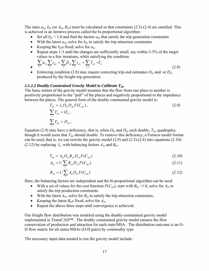
2.1.2 Freight Distribution The freight generation task is followed by freight distribution. Freight distribution is to distribute freight generation (production and attraction) of a state to all other states. The freight distribution can be modeled using two different methods – the doubly constrained growth factor method and the doubly constrained gravity model. The two methods are explained in the following section.

2.1.2.1 Doubly Constrained Growth Factor Methods to Calibrate Tijn The growth-factor model directly uses the observed base-year freight data, tijn, oin and djn, and forecasted future-year freight production and attraction, Oin and Djn and freight growth factors to calibrate Tijn. This model is simple and practical, however, transportation costs are not considered in this model. From 2.1, we have the following flow conservation relationships: For future year: in

jijn OT =∑ (2.3)

jni

ijn DT =∑ (2.4)

For base year: in

jijn ot =∑ (2.5)

jni

ijn dt =∑ (2.6)

These flow conservations require two sets of different growth factors between future year and base year for freight trips in and out of each state or MSA. The best methods can be found in [26], whose work was later extended by [27], [28] and [29] for the gravity model. Define: inininijnijn oOtT α== // , origin (state or MSA) i specific growth factors

jnjnjnijnijn dDtT β== // , destination (state or MSA) j specific growth factors inA , jnB , balancing factors for i and j ininin Aa α= , jnjnjn Bb β= , freight growth rates for i and j Therefore, we have: jninijnijn batT = , (2.7)

17

The rates ain, bjn (or Ain, Bjn) must be calculated so that constraints (2.3)-(2.4) are satisfied. This is achieved in an iterative process called the bi-proportional algorithm:

• Set all bjn = 1.0 and find the factors ain that satisfy the trip generation constraints • With the latest ain, solve for bjn to satisfy the trip attraction constraints • Keeping the bjns fixed, solve for ain • Repeat steps 1-3 until the changes are sufficiently small, say within 3-5% of the target

values in a few iterations, while satisfying the condition:

• n

jiijn

jijn

jjn

jijn

iin TTtt ∑∑∑∑∑ ===

,βα

(2.8) • Enforcing condition (2.8) may require correcting trip-end estimates Oin and/ or Djn

produced by the freight trip generation.

2.1.2.2 Doubly Constrained Gravity Model to Calibrate Tijn The basic notion of the gravity model assumes that the flow from one place to another is positively proportional to the “pull” of the places and negatively proportional to the impedance between the places. The general form of the doubly constrained gravity model is: )( ijnjninnijn CFDOT λ= , (2.9)

inj

ijn OT =∑ ,

jni

ijn DT =∑ ,

Equation (2.9) may have a deficiency, that is, when Oin and Djn each double, Tijn quadruples, though it would seem that Tijn should double. To remove this deficiency, a Furness model format can be used, that is, we can rewrite the gravity model (2.9) and (2.3)-(2.4) into equations (2.10)-(2.12) by replacing nλ with balancing factors Ain and Bjn. )( ijnjnjnininijn CFDBOAT = (2.10)

∑=j

ijnjnjnin CFDBA )(/1 (2.11)

∑=i

ijnininjn CFOAB )(/1 (2.12)

Here, the balancing factors are independent and the bi-proportional algorithm can be used: • With a set of values for the cost function F(Cijn), start with Bjn =1.0, solve for Ain to

satisfy the trip production constraints • With the latest Ain, solve for Bjn to satisfy the trip attraction constraints, • Keeping the latest Bjns fixed, solve for Ain • Repeat the above three steps until convergence is achieved.

Our freight flow distribution was modeled using the doubly-constrained gravity model implemented in TransCAD™. The doubly constrained gravity model ensures the flow conservation of production and attraction for each state/MSA. The distribution outcome is an O-D flow matrix for all states/MSAs (O-D pairs) by commodity type. The necessary input data needed to run the gravity model include:

18

• A state/MSA-to-state/MSA friction factor matrix or an impedance table. In our distribution, a distance-based friction factor matrix was used.

• A USA state/MSA zone layer with estimated productions and attractions from freight generation

• A layer of state/MSA population-weighted centroids The friction factor matrix is based on a state/MSA-to-state/MSA centroid distance matrix, which is commonly calculated in a mathematical function, such as gamma, exponential, or inverse power. The distance matrix itself can also be used as the input friction factor matrix. Since the regression estimated production and attractions include within state/MSA productions and attractions, each of these estimated productions and attractions were multiplied by a “in-state/MSA factor”. The in-state/MSA factor ensures that a state/MSA distributes its relevant production to all other states/MSAs and attracts from other states/MSAs the relevant freight that is distributed to the state/MSA. Using the in-state/MSA factor, the total in-state/MSA production and attraction were computed as an average of the in-state/MSA production and attraction.

2.1.3 Freight Modal Split Model After freight distribution, the next step in the traditional freight-modeling framework would be to perform mode split. Mode split is where the distributed flow is split among the available modes. Many algorithms have been used to represent decision-making for mode selection ranging from an easy and coarse method to a more complicated and detailed one. The easiest method is to use empirical data to develop the ratios of sharing among modes. Another possible way is to construct a diversion curve describing the relationship between proportions of flows by mode against the difference of some factors (e.g. cost or time difference) between any two modes. In this project, we used, for the sake of simplicity, the ratios of sharing among modes and assumed that the ratios among modes in future years will be the same to those of the base year. The output of the modal split step is the freight flow by O-D pair by commodity pair by mode.

2.1.4 Freight Flow Assignment Model The major purpose of a freight assignment model is to predict the freight-flow patterns between the given O-D pairs on a transportation network. The model distributes the freight flow on the network either by shortest routes or by a set of constraints related to the capacity, time, and cost of the network links. The assumption for the assignment is that carriers seek to minimize the time or cost associated with their chosen routes. There are several algorithms used for finding the shortest path in un-capacitated assignment. Similarly for the capacitated assignment, since the original formulation of the traffic assignment problem [16], many algorithms for its solution have been presented [17]. The capacitated assignment is based on the assumption that carriers seek to minimize the cost associated with the chosen route. The cost could be in terms of travel time, monetary cost or any other measure of disutility. The research team developed two alternate models for freight assignment. The first one is the regional model, and the second one is the combined regional-state model. They are explained in the following paragraphs.

19

In the regional model, the spatial unit is the state/MSA in the US. The input to this step is the results of the modal split. Such a model with just a few regions (only one if the state is the spatial unit and 3 if MSA is the spatial unit) in Oklahoma can be used to ascertain the through-flow in the state. This would mean that the results of the freight assignment do not give sufficient information to make infrastructure-planning decisions for the state of Oklahoma. The research team had initially planned to use this information from the regional model as an input to a detailed state model (county level in Oklahoma) for further analysis. But, by the time the regional model was completed, it had become apparent that this approach was not the best way forward for the team. It also became clear that a more detailed methodology was required to accurately model the traffic in the state. The research team developed the second model called the combined regional-state freight movement model. The spatial units in this model include the state/MSA for states other than Oklahoma and the counties in Oklahoma. Irrespective of the spatial unit, the team had the task of converting the freight data in the state of Oklahoma from the state/MSA level to the county level. If the spatial unit is a state, then the freight data has to be split among the 77 counties in Oklahoma. On the other hand, if the MSA is the spatial unit, the state of Oklahoma had three regions – the Oklahoma City region, the Tulsa region and the remainder of Oklahoma. It was observed that the Oklahoma City and Tulsa regions consisted of 8 counties each in Oklahoma, while the remainder of Oklahoma region was comprised of the remaining 61 counties. As a result, the freight flow in each of these three MSA regions has to be split into the constituent counties. This process required the population and employment data by industry code for each county. This means that the inputs to this model include the freight data at the state/MSA level, and the population and employment data by industry code by county level in Oklahoma. The result of this step gives us the freight data at county level in Oklahoma and at the state/MSA level in the other states. This data would serve as the input to the freight assignment for the combined regional-state model. This gives us a detailed model, and the results of the flow assignment would provide us the information required for making infrastructure planning decisions. It can be seen from the Figure 2.1 that the four-step approach can be used for both the approach irrespective of the number of regions (50 regions if the state is the spatial unit or 114 if the MSA is the spatial unit). The research team performed both capacitated as well as un-capacitated flow assignments on the combined regional-state model for the highway network and un-capacitated flow assignments on the railway and waterway network. The various capacitated and un-capacitated freight assignment methods are summarized in the following section. The all-or-nothing assignment is an un-capacitated flow assignment method, while the system optimal, user equilibrium, and stochastic user equilibrium are capacitated flow assignments.

2.1.4.1 All–or–Nothing Assignment All-or-Nothing Assignment is an example of the un-capacitated flow assignment. It uses the shortest paths connecting origins and destinations to assign all traffic flows between O-D pairs. It is called all-or-nothing because either all of the traffic from node i to j moves along a route or it does not; there is no splitting of traffic between two or more routes. The model uses only one shortest path between every O-D pair without considering the time delay caused by volume on the link or the capacity of the link. Even if there are two or more paths with almost similar travel

20

time or cost, it only uses one of them to do the assignment making the assignment unrealistic for real world scenarios.

2.1.4.2 System Optimal Assignment The basic assumption of the system optimal assignment is that the “drivers cooperate with one another in order to minimize total system travel time” (Wardrop’s second principle). In this model, the congestion is minimized by telling the drivers which route to use. It may not be a behaviorally realistic model, but transportation planners can use this model to manage the traffic, minimize the travel costs and hence achieve an optimum social equilibrium. The system optimum equation tries to minimize the flow related travel time on link “a”. It is subject to two conditions; the first condition ensures that summation of the flow on path “k” connecting Origin-Destination pair (r-s) for all “r” and “s” is equal to the freight rate between “r” and “s”. The second condition sets the equilibrium flows on link “a” equal to summation over “r”, “s”, “k” of the flow on path “k” connecting “r-s” times δ (which equals to 1 if link “a” is on path “k” and 0 if otherwise). Also, the flow on path “k” connecting “r-s” should be greater than or equal to zero for all “k”, “r” and “s”. Equilibrium flow on link “a” should be greater than or equal to zero for all “a” belonging to set of 0 and all positive numbers ([18], [19]).

2.1.4.3 User Equilibrium Assignment The user equilibrium (UE) assignment model is based on Wardrop’s first principle and uses an iterative process to achieve a convergent solution, in which no travelers can improve their travel times by shifting routes (Travel Demand Modeling with TransCAD™ 4.8). The deterministic user equilibrium is achieved by assuming that the drivers have perfect knowledge about travel costs on a network and so they choose the best route for them. The equilibrium criteria is met when all the paths carrying no flow have travel time greater than (or equal to) those carrying the flow so that no traveler can reduce his travel costs by unilaterally changing routes. The equation is a “simple flow conservation equation and non-negativity constraint” where the objective is to minimize the summation of the integral of travel time by equilibrium flows on link “a” over all link “a”. It is subject to the same two conditions as in the system optimum equation; the first condition ensures that the summation of the flow on path “k” connecting the Origin-Destination pair (r-s) for all “r” and “s” is equal to the freight rate between “r” and “s”. The second condition sets the equilibrium flows on link “a” equal to summation over “r”, “s”, “k” of the flow on path “k” connecting “r-s” times δ (which equals 1 if link “a” is on path “k” and 0 if otherwise). Also, the flow on path “k” connecting “r-s” should be greater than or equal to zero for all “k”, “r” and “s”. Equilibrium flow on link “a” should be greater than or equal to zero for all “a” belonging to the set of 0 and all positive numbers ([18], [19], [22], [23]).

2.1.4.4 Stochastic User Equilibrium Assignment The concept of Stochastic User Equilibrium (SUE) was introduced by [20] Daganzo and Sheffi in 1977. SUE assumes that the perception of total cost of a link varies from one traveler to another as they do not have all information concerning network attributes. A SUE assignment is an updated version of UE model, which makes use of both the less attractive as well as the most attractive routes. In the SUE assignment, the less attractive route has some flow, unlike the zero flow in UE assignment. The detailed mathematical formulation of SUE can be found in [21].

21

2.2 Timeline of the Freight Movement Modeling Project Figure 2.2 presents the timeline of the project, highlighting the major accomplishments during each year of the project.

Figure 2.2: Freight Movement Modeling Project Timeline

During the first phase (2003) of the project, the research team focused on developing the freight movement modeling methodology and identifying the various data sources. Initially, the team chose to use a two-tier model with the regional model at the first tier and the state model at the second tier using the four-step approach. The team simultaneously worked on identifying various publicly available databases for obtaining the data such as freight flow data, socio-economic data and transportation infrastructure development data. The math models for predicting the regional freight flow were developed during the second phase of the project between 2003 and 2004. The math models developed during the second phase were validated during the third phase from 2004–2005. During the second part of the third phase (2005–2006), the emphasis was on developing the proof-of-concept software prototype for the regional model. During this phase, the research team had identified that the two-tier model was not the best model. So a new approach called the combined regional-state model was developed during Phase IV (2006-2008). The FAF2 database provided the freight data by O-D pair by commodity by mode. Therefore, the team used the available data to provide a proof-of-concept implementation for the combined regional-state model. This meant that the first three steps of the four-step model (freight generation, freight distribution, and modal split) were not redone at the MSA level. The final year of the project, 2008, focused on developing the proof-of-concept software prototype for the combined regional-state model.

22

3. IDENTIFICATION OF DATA SOURCES AND ISSUES WITH AVAILABILITY AND PREPARATION OF DATA

Building a freight movement model involves several steps. Having developed the methodology, the team had to identify data sources that present adequate and reliable data. This step would also include identifying various issues like data availability, missing data, and preparation of input data for analysis.

3.1 Identification of Data Sources This section deals with the identification of reliable data sources. Various forms of inputs required for the models include flow data, network information for the three modes (highway, waterway, and railway), and socio-economic data. These data come from a wide range of publicly available databases. This section of the report includes a classification of the data sources used thus far and a description of the application of the data contained in these databases at the appropriate places in the multi-step modeling approach.

3.1.1 Classification of Data Sources Based on the nature of the databases and their application, the databases have been classified into three categories. There are many public/commercial databases falling into the three categories. The schematic representation is shown in Figure 3.1.

Figure 3.1: Classification of Data Sources

3.1.1.1 Commodity Flow Databases These types of databases quantify/describe the flow of commodities based on various attributes such as origin, destination, mode, reliability, weight, dollar value, distance shipped, etc.

3.1.1.2 Auxiliary Databases These types of databases quantify the factors that are either responsible for the generation of freight flow or are affected by the change in freight flow. They cover socio-economic areas like businesses, manufacturing, and trading which may contribute to the flow of freight and include demographic data like population, income and other socio-economic factors.

INPUT DATABASE IN FREIGHT TRANSPORTATION PLANNING

Commodity Flow • Commodity Flow

Survey (CFS) • Trans-Search Database • Rail Waybill Database • Freight Analysis

Framework (FAF2)

Auxiliary Database • Census.gov • Economic Census • County Business

Pattern (CBP) • Transportation Satellite

Accounts (TSA) • Annual Survey of

Manufacturers

Network Database • National Transportation

Atlas Database (NTAD) • TIGER Database • National Highway Planning

Network (NHPN) • Federal Railroad

Administration (FRA) • Federal Highway

Administration (FHWA) • Bureau of Transportation

Statistics (BTS)

23

3.1.1.3 Network Databases These types of databases contain geographic network of routes by different modes of transportation (highway, railway, and waterway) and also quantify attributes such as travel time and distance.

3.2 Issues with Data Availability and Preparation of Input Data We summarize in sections 3.2.1 through 3.2.6 several issues related to the availability and preparation of various types of input data.

3.2.1 The Base Year Selection During the preliminary stages of model development, many relevant databases were found to have different base years and dates of completion. For example, Commodity Flow Survey (CFS) was collected for years 1987, 1993, 1997 and 2002. The economic census was collected for 1992, 1997 and for years ending in 2 & 7. The population census is collected for 1990 and 2000. County Business Flow Pattern is reported annually by the BTS. The FAF2 database has the flow information from origins to destinations by modes for 2002 and 2005 to 2035 in 5-year increments. Since many databases were publicly available for the year 2002, it was decided to use 2002 as the base year for combined regional-state model development.

3.2.2 Developing Commodity Groups Vehicle traffic levels are derived from the movement of commodities. Thus, a good understanding of the commodities is necessary. Forecasting single commodity/product raises many issues about forecasting accuracy, data requirement, and complexity. Forecasting groups of commodities provides reasonable forecast accuracy. Though a large number of groups provide precision, they increase the complexity of model development. The Standard Classification of Commodity Groups (SCTG) developed by the Bureau of Transportation Statistics (BTS) provides the base for the level of commodity grouping needed. The SCTG codes [25] are available at 2-digits (43 commodity groups) to 5-digits detailed level (more than 300 commodity groups). Since, the 2-digit SCTG codes strike the balance between the number of commodity groups to model and data availability; they are used in the model development. Commodity groups can be categorized as Consumer Goods (directly consumed by the consumer), Industrial Goods (goods that require further processing to become consumer goods or goods that are used by the industries directly), or both (used by consumers and industry in varying proportions). The 2-digit SCTG codes are grouped based on the categorization above. For example, Transportation Equipment (SCTG 37) is an industrial good. Alcoholic beverages and tobacco products (SCTG 08-09) are consumer goods. Electronic /electrical components and office equipment (SCTG 35) belong to the third category; part of it (electric generators, telephone switching apparatus, etc.) is used by the industries and the remainder (electronic entertainment products like CD players, TVs, etc.) is used by consumers directly. Though, the commodity groups are categorized, the forecasting or further analysis will be done for 2 digit commodity groups. A complete list is given in Table A.1 (Appendix A). The categorization is expected to help in model development by taking advantage of commonality in the factors that influence the production and/or the attraction of commodity groups within a category.

24

3.2.3 Relating Commodity Groups to Industrial Sectors or Economic Indicators The 1997 Economic Census data are classified primarily on the 1997 North American Industry Classification System (NAICS), and, to a lesser extent, on the 1987 Standard Industrial Classification (SIC) system used in previous censuses [5]. NAICS defines industries to a sixth digit. The 1997 Economic Census covers 1,057 of the 1,169 industries in NAICS but there are some exclusions in data. Some of these exclusions are covered in County Business Patterns (CBP) and four of these data will be included in the 2002 Economic Census. Table A.2 (Appendix A) gives a list of data exclusions [5]. We now explain the methodology to create a mapping between industry groups and commodity groups. Commodity Flow Surveys (CFS) obtains data on shipments by domestic establishments in manufacturing, wholesale, mining, and selected other industries according to the STCG system, while the 1997 Economic Census presents data classified according to both the 1987 Standard Industrial Classification (SIC) system and 1997 North American Industry Classification System (NAICS), there is not a direct or one-to-one correspondence between the two coding systems as a particular commodity could be contributed by one or more industry and vice versa. For example, freight generated from cigarette paper manufacturing could contribute to both the printed product industry and tobacco product industry. Therefore, a code mapping procedure is proposed and carried out at this stage to find the links between the SCTG commodity groups and NAICS/SIC industry groups. Although Economic Census data has two classification systems, namely the NAICS and SIC, many of the individual SIC industries correspond directly to industries as defined under the NAICS system. But most of the higher level SIC groupings do not have a direct correspondence to NAICS. Care should be taken in comparing data for retail trade, wholesale trade, and manufacturing, which are sector titles used in both NAICS and SIC, but cover some what different groups of industries [5]. Fortunately, a bridge file between NAICS and SIC classification is available from the Census Bureau. It demonstrates the relationship between NAICS and SIC by showing data for the lowest common denominators between the two systems. The research team had to find the mappings from SCTG to NAICS and use the bridge file to find mappings from NAICS to SIC, when necessary. Detailed definitions of SCTG commodity and NAICS industry classifications are obtained from the Economic Census. Starting with a commodity and using keywords that are found in the definitions, the commodity was matched to its associated contributing industry at the 6-digit NAICS level. Keyword matching could be done using the 1997 Economic Census software available in CD-ROM [6] from the Census Bureau. There is an option where the user could type in a keyword to search for the NAICS industry. A 6-digit level data is of little use as there are always missing data issues at such a detailed level in the 1997 Economic Census statistics. Hence, aggregated 3-digit NAICS data was extracted for use in the multiple regression models in the case of the regional model. Figure 3.2 presents the code mapping procedure in the form of a flow chart, while the schematic in the Figure 3.3 shows an example of the code mapping procedure to find the associated industries that may contribute to tobacco products. A summary for the code mapping results is presented in Table A.3 in Appendix A.

25

Figure 3.2 Code mapping (algorithm)

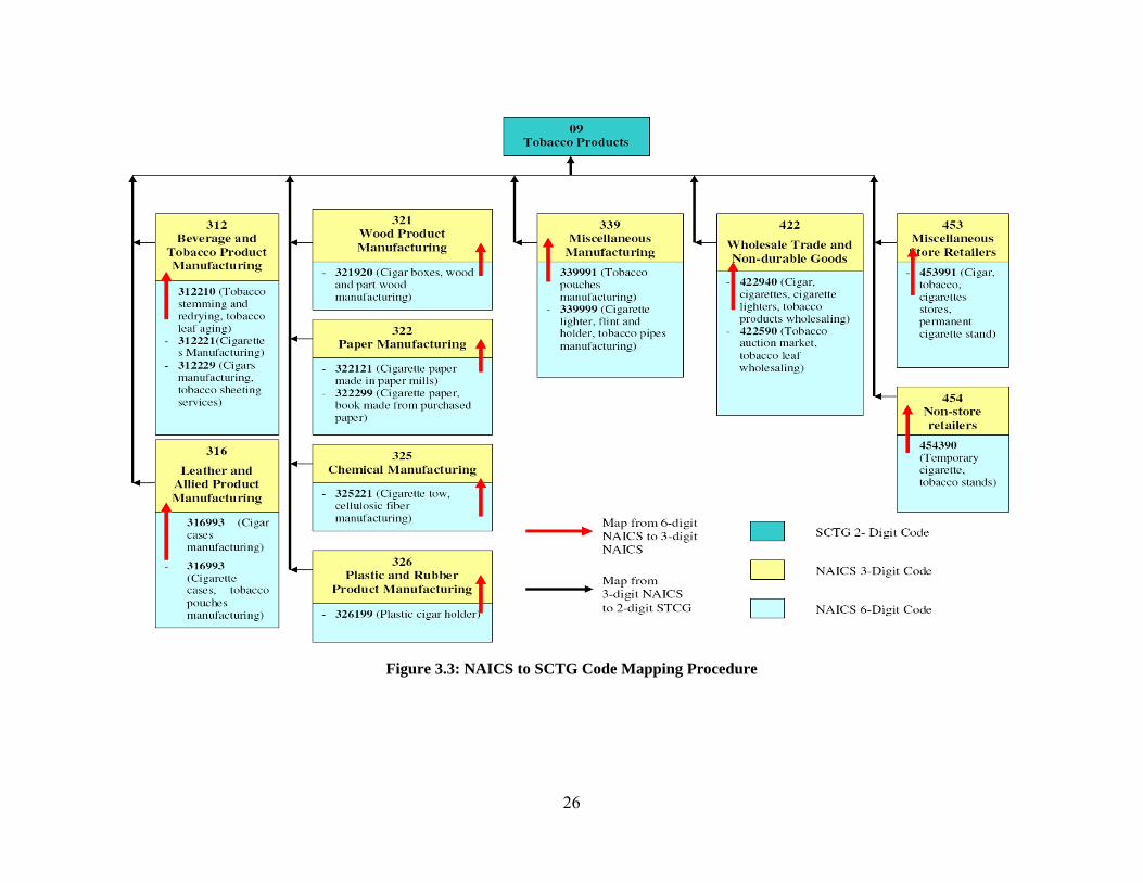
26

Figure 3.3: NAICS to SCTG Code Mapping Procedure

27

3.2.4 Finding the Commodity Flows Origin and destination data for the commodities must be obtained to build a factual model. There are many data sources to obtain the flow data. Two mostly citied databases in other efforts on statewide freight movement model [7, 8] are Commodity Flow Survey (public domain) and TRANSEARCH® (commercial). The flow details in CFS at the state level have just enough detail for our model development. The CFS database was used during the development of the regional model. But, it was found that the database has some issues with missing freight flow data. At this stage, the research team came across a new source of freight flow data “Freight Analysis Framework 2 (FAF2)” developed by the Federal Highway Administration (FHWA), in cooperation with the Bureau of Transportation Statistics (BTS) through Oak Ridge National Laboratory and MacroSys Research and Technology [13]. Basically, the FAF2 database is the adjusted version of CFS 2002 by using techniques such as Iterative Proportional Fitting and Log Linear modeling to fill the missing data in CFS 2002. The freight data of all commodities for about 50 O-D pairs were compared (between the databases) and it was found that the data is consistent. As a result, the FAF2 freight flow database was identified as a better alternative to the CFS database.

3.2.5 Finding the Socio-Economic Variables The commodity flows are derived from demand. These flows depend on other social factors, economic factors, technological developments, etc. The social variables include population estimates for the base year, median household income and disposable income. The economic variables include details about the number of industrial establishments, employment and revenue/sales. Such data are available from Census data (population and economic) published by the U.S. Census Bureau, County Business Pattern by BTS and Regional Economic Information Systems (REIS) by Bureau of Economic Analysis (public domain) and IMPLAN economic databases (commercial). The social and economic census data is the major data source for the independent variables used in the regional model development (discussed in Appendix B) as well as in the development of the combined regional-state model (discussed in Section 4.2.2).

3.2.6 Finding the Network Information The prime database sources of the highway network are the National Transportation Atlas Database (NTAD), National Highway Planning Network (NHPN) database, GIS database provided by ESRI, Tiger database provided by Census and FAF1 and FAF2 provided by the Federal Highway Administration database. The research team used the FAF2 database, which has the necessary attributes like the network’s capacity, free flow speed and travel time. Apart from the input attributes necessary for capacitated assignment, the database is also compatible with the freight data. The database was developed from the NHPN Version-3 database developed by the Federal Highway Administration to support GIS based traffic modeling and mapping. The primary source for the railway network is the Federal Railroad Administration (FRA) and Bureau of Transportation Statistics (2006), “National Waterway Network”, National Transportation Atlas Databases (NTAD). The primary source of the waterway network is the Vanderbilt Engineering Center for Transportation Operations and Research and Bureau of Transportation Statistics “National Rail Network”, National Transportation Atlas Databases 2006 (NTAD). The research team used the railway and waterway networks developed by NTAD and available from the BTS website [9, 10].

28

4. COMBINED REGIONAL-STATE MODEL The regional freight movement model, developed during Phases II and III, has been discussed in detail in Appendix B. In the current chapter, the discussion will be about the combined regional-state model, which was developed during the final phase of the FMM project.

4.1 Significance of the Combined Regional-State Model The FAF database contains commodity flows for the fifty states in the US plus the DC region. Each individual state is either treated as one region or is divided into a number of Metropolitan Statistical Areas (MSAs), and the remainder of the state (see Table C.1 in Appendix C). In total, there are totally 114 centroids of the states and MSAs in the US. The state of Oklahoma is divided into three different MSAs, namely, the Oklahoma City region, the Tulsa region and the remainder of Oklahoma region. This would mean that at the MSA-level granularity the results of the freight assignment within Oklahoma may not have sufficient information to support infrastructure planning decisions for the state of Oklahoma. Therefore, to perform a more detailed analysis of freight in the state of Oklahoma, there is a need to look at the flow assignments at least at the county level. This requires the splitting of the flow from the MSA level to the county level within the state of Oklahoma. It can be seen that the Oklahoma City region records data for eight counties, while the Tulsa region records data for eight counties. The remaining sixty one counties are recorded under remainder of Oklahoma. The list of counties that fall under the MSAs and the remainder of OK are summarized in Tables C.2, C.3 and C.4 respectively (see Appendix C). In the combined regional-state model, our approach combines the 114 centroids of the states and MSAs with the 77 counties in Oklahoma. Such an approach would require splitting the regional freight flow data into the county level data. With the county-level freight data, we have a model that can predict flow volumes by commodity type and by mode and route for incoming, outgoing, within and through freight flows for the Oklahoma counties. Figure 4.1 presents the FAF2 regions. Figure 4.2 presents the FAF2 regions along with the 77 counties in Oklahoma.

Figure 4.1: FAF2 regions

29

Figure 4.2: FAF2 regions with 77 counties in Oklahoma

The methodology involved in the preparation of the data is presented in the following sections.

4.2 Preparation of Network Data for Flow Assignment The preparation of network data depends on the mode of freight flow. This is because of the fact that certain attributes of the network are considered for one mode, while they are not for another. For example, we consider the capacity information in the case of the highway network, while the same attribute is not considered for waterway and railway networks. These issues are discussed in detail in the following sub-sections.

4.2.1 Highway Network Freight Analysis Framework version-2 (FAF2) Highway Link database (FAF 2.2) comprises of 170,773 links of various lengths in TransCAD™ format. Out of these links, 367 links are part of the Canadian highways (connecting the continental US to Alaska). The attributes of the highway links include the length, name of the roadway, state abbreviation, state and county code and one to three signage for each of the links. Other than these attributes which give general description about the location of the link, there are a few other attributes which categorize them in different groups. The ‘STATUS’ categorizes the links in groups like proposed, open to traffic, ferry route and Canadian routes. The ‘LINK_TYPE’ gives information about the FAF2.2 links as follows: 0 = Other FAF 2.2 routes 1 = State truck route not on the National Network. 2 = National Network (NN) route 5 = No trucks allowed These links are categorized by functional classification (FCLASS) ranging from 1-19, where FCLASS is set as: 1 = Rural principal arterial - Interstate 2 = Rural principal arterial - Other 6 = Rural minor arterial 7 = Rural major collector 8 = Rural minor collector 9 = Rural local 11 = Urban principal arterial - Interstate 12 = Urban Principal Arterial - Other freeways and expressways 14 = Urban principal arterial - Other

30

16 = Urban minor arterial 17 = Urban collector 19 = Urban local - (Blank) = Data not available The first step in network preparation is to create centroids for all the regions in the FAF2 database as well as the 77 counties in Oklahoma (see Figure 4.2). The geographic centers of the regions are set as the centroids and are prepared using the ArcGIS software. The centroids are stored as a separate layer file. The next step is to connect the centroids to the network link using centroid connectors. This task was performed by using the “Tools-Map Editing –Connect” tool in TransCADTM, which allows the connection of points in one layer to the nodes or lines of another layer. In this case, the centroid is connected to the network using the shortest connection. Since the centroid connector can connect the centroid to any point on the nearest existing link in the network, that link is now split into two different links. While one of these two links maintains the old ID, the other one will have a new ID. The rest of the attributes (other than the length of the link) can be retained in both the links by using an option that allows copying the attributes of the old link to the new link created after the connection [11]. Another issue that needs to be sorted is that the capacity and free-flow travel time information are furnished for only the original links. For the centroid connectors and split links, there was a need to calculate the free flow times and the capacities. The free flow times were calculated using the link performance function provided by Bureau of Public Roads [32]. The link performance function relates link travel time as a function of volume by capacity ratio (VCR) as follows.

⎥⎥⎦

⎤

⎢⎢⎣

⎡⎟⎠⎞

⎜⎝⎛+=

β

αCVTT ffcon 1 (4.1)

where, Tcon Congested link travel time Tff Free Flow link travel time V Volume on the link C Capacity of the link α Calibration parameter = 1.5 β Calibration parameter = 4.0 The database has the congested travel time, volume and capacity. These three values were used to calculate the free flow time by using the following formula.

⎥⎥⎦

⎤

⎢⎢⎣

⎡⎟⎠⎞

⎜⎝⎛+

=β

αCV

TT conff

1

(4.2)

The resulting free flow speed obtained from the above method was not rational and thus the free flow time was calculated as follows.

31

ff

ff SLT = (4.3)

where, L Length of the link Sff Free Flow speed on the link The next task is to assign the capacities to the centroid connectors, the split links as well as the 367 links in Canada (which connect Continental US to Alaska). The centroid connectors were given a capacity of 23,000, which is higher than the highest capacity on the highway route. The 367 links in Canada are given a capacity of 5,561, which is the average of the capacity for the Interstate highways (with functional classification of 11) in the US. The remaining links are categorized as per their functional classification and RU code. An average capacity was calculated for all the other links having the same functional classification and RU code and this value was assigned as the capacity for the links in that category. With the updated database, the new highway network (see Figures 4.3 and 4.4) was built.

Figure 4.3: US Highway Network – Continental US

32

Figure 4.4: US Highway Network – Alaska and Hawaii

4.2.2 Railway Network Railway network (Rail_Net) is prepared using NTAD 2006 (Rail2m_06 layer representing the railway network, 17,092 links) and IMP_R&T layer (Inter-modal points including the truck and rail terminal nodes, 2,270 links). IMP_R&T points and the Rail2m_06 layer were connected if the railway was within a 5 mile distance. The points that were not within 5 miles were selected and manually connected to the railway network. We connected the centroids with the links below IMPs not with the network directly. Finally, centroids and Oklahoma centroids were connected to the Rail_Net using the node (centroid) selections that were within a 50-mile distance of railway network. Finally, the result was a railway network composed of 21,456 links (see Figure 4.5).

Figure 4.5: US Railway Network

33

4.2.3 Waterway Network The waterway network was prepared using the NTAD 2006 network, which originally had 6,277 links. Truck-Port-Rail (340 links), Rail-Port (10 links), and Port-Truck (112 links) inter-modal points (IMPs) were connected to the waterway network; afterwards IMPs were connected to the centroids. Finally, the number of links in the waterway network was 7,289 (Figure 4.6 and Figure 4.7). Freight data was prepared from the FAF2.2 database (DOM_KT table), which has a total of 760 corresponding records. Oklahoma is represented by 3 points in the waterway network, although Oklahoma only has waterway connection only in Tulsa.

Figure 4.6: US Waterway Network

Figure 4.7: US Waterway Network – Alaska and Hawaii

34

Figure 4.8 presents the different steps in the preparation of the network data for the three modes.

Figure 4.8: Preparation of Network Data

4.3 Preparation of Freight Data FAF2 database provides the freight data by tonnage either for the whole state or for a few MSAs and the remainder part of the state. A heuristic method was developed to split this regional-level freight data into county-level data. The employment by commodity is used for the production data, while the county-wise population is used for the attraction data to split the freight data from the regional level to the county level. The assumption behind the use of these socio-economic factors is that production of any commodity is directly related to the number of employees working to produce that commodity and the attraction of any commodity is directly related to the population of that area.

No

Yes

No

YesIs mode = highway

Capacitated Flow

Assignment? Identify inter-modal points and

connect to the network

Add Centroid layer

Add Centroid Connectors

Connect centroid to the inter-modal

points

Calculate free-flow travel times for links with missing data

Set capacity for links with missing data

Highway / Railway / Waterway Network

Modified Highway / Railway /

Waterway Network data

35

4.3.1 Code Mapping Code mapping (discussed in detail in Section 3.2.3) is a methodology that helps to bridge the commodity codes (SCTG) with the industrial codes (NAICS). The main purpose of the bridging is to relate each of 2-digit SCTG codes with 4-, 5-, or 6-digit NAICS codes by their relevancy so that the employment involved in producing each of the commodities can be acquired. The employment data is available by Industrial codes only. The bridging helps to find a more accurate estimate of the number of employees involved in producing any one commodity. The bridge between 2-digit SCTG codes and 4-digit NAICS codes were first developed for the Regional model, a few years ago. Recent revisions of the mapping showed that at 5- or 6-digit level, some of the codes are not related to the commodity it is being mapped with. A new mapping was thus developed to map the 2-digit SCTG codes with 5- or 6-digit NAICS codes. The final result is a complete mapping between the commodities and the industrial codes that are directly or indirectly involved in the production of that commodity (See Chapter 3 for an example of code mapping). Figure 4.9 presents the code-mapping scheme.

Figure 4.9: Code Mapping Scheme

4.3.2 State to County Split for Oklahoma The freight production and attraction for three regions of Oklahoma are split into production and attraction for the seventy-seven counties of Oklahoma using the following procedure. The employment information by commodity and the population information by county are used to split the production and attraction from the regional level to the county level flow. The County Business Pattern (CBP) provides the employment for each industry at the county level by NAICS codes. The CBP records the employment for all of the counties within the US from 1994 to 2005. It gives the employment by state, county, zip code and metro level. The data is by SIC codes from 1994 to 1997 and then by NAICS codes from 1997 to 2005. The website provides information like the number of employees, payroll and number of establishments for each of the counties. The bridging between SCTG and NAICS codes sets up a list of industries directly or indirectly related in producing a commodity. Then the 2002 employment for each of those industries related to a commodity is extracted from the CBP website. This gives the employment data for that particular commodity. Similarly, employment data is extracted for all the commodity types.

36

The issue with this data is that most of the time the employment for a specific industry for a specific county is given as a range. For such data where a range is provided, the average is extracted and used as the employment data. Then again, the average is calibrated with the total employment using the following formula:

∑⋅=

=

77

1ii

OKii

Emp_Ori

EmpEmp_OriEmp_Cal (4.4)

where, Cal_Empi Calibrated employment in county i Ori_ Empi Original employment in county i EmpOK Total employment in Oklahoma The 2002 population for each county in Oklahoma is obtained from the census database. The population data for each county as well as the employment for each commodity in each county are used to divide the state level production and attraction flows to the county level. However, before splitting the state flow to the county flow, the total flow is separated into four categories, depending on whether they are produced in Oklahoma or attracted to Oklahoma or if they are neither produced nor attracted to Oklahoma or if they are both produced and attracted to Oklahoma. The “From” flow is used for all the flows produced in Oklahoma (i.e., they originate from Oklahoma) and are attracted to the states outside Oklahoma. The “To” flow refers to all the flows which are produced outside Oklahoma (i.e., they originate outside of Oklahoma) but are attracted to (consumed in) Oklahoma. The “Within” flow refers to all the flows that are both produced in Oklahoma and also attracted to Oklahoma. The last type of flow, the “Through” flow, is both produced and attracted outside of Oklahoma, but which uses the highways of Oklahoma while transporting those goods from origin to destination. This separation of flows by O-D pairs helps in determining whether to use employment or population ratio for split. The employment ratio is used to split the “From” flow, while the population ratio is used to split the “To” flow. In the case of the within flow, the employment ratio is used first to split the production followed by the population ratio to split the attraction. FAF2 database provides flow information in Oklahoma as flows in the three geographic parts – Oklahoma MSA, Tulsa MSA and the remainder of Oklahoma. The Oklahoma MSA and Tulsa MSA consist of eight counties each and the remainder consists of sixty one counties. In order to split the production and attraction for Oklahoma flows we use the following formula: Production (of a commodity) from County ‘i’ in Oklahoma MSA: POKC

i = POKC * EMPOKCi

EMPOKCi

i=1

8

∑ (4.5)

37

Production (of a commodity) from County ‘j’ in TULSA MSA: PTUL

j = PTUL * EMPTULj

EMPTULj

j=1

8

∑ (4.6)

Production (of a commodity) from County ‘k’ in OK REM: PREM

k = PREM * EMP REMk

EMP REMk

k=1

61

∑ (4.7)

Flow (of a commodity) from County ‘i’ (OKC) to county ‘j’ (TULSA) or ‘k’ (OK REM):

Fij = POKC

i * POPTULj

POPTULj

j=1

8

∑Fi

k = POKCi * POPREM

k

POPREMk

k=1

61

∑ (4.8)

Flow (of a commodity) from County ‘j’ (TULSA) to county ‘i’ (OKC) or ‘k’ (OK REM):

Fji = PTUL

j * POPOKCi

POPOKCi

i=1

8

∑Fk

j = PTULj * POPREM

k

POPREMk

k=1

61

∑ (4.9)

Flow (of a commodity) from County ‘k’ (OK REM) to county ‘i’ (OKC) or ‘j’ (TULSA):

Fki = PREM

k * POPOKCi

POPOKCi

i=1

8

∑Fk

j = PREMk * POPTUL

j

POPTULj

j=1

8

∑ (4.10)

Attraction (of a commodity) to County ‘i’ in OKC: AOKC

i = AOKC * POPOKCi

POPOKCi

i=1

8

∑ (4.11)

Attraction (of a commodity) to County ‘j’ in TULSA:

∑=

= 8

1

*

j

jTUL

jTUL

TULj

TUL

POP

POPAA (4.12)

Attraction (of a commodity) to County ‘k’ in OK REM:

∑=

= 8

1

*

j

jREM

jREM

REMj

REM

POP

POPAA (4.13)

where, P Production

38

A Attraction EMP Employment POP Population i County in Oklahoma City MSA j County in Tulsa MSA k County in Remainder of Oklahoma

4.3.3 Tonnage to Truck Conversion FAF2 database provides the freight data in terms of either tonnages or dollar values. While performing the all-or-nothing assignment, the unit of freight flow does not matter. This means that there is no need for any special data preparation when we perform flow assignment on the railway and waterway network as well as the all-or-nothing assignment on the highway network. But, while performing the capacitated assignment on the highway network, there is a need for some data preparation. The FAF2 database provides the capacities on the links in terms of number of trucks. This necessitates that the freight data in tonnages be converted to number of trucks. This conversion can be done using payload factors. For each commodity or a group of similar commodities, the average payload factor is derived and then the tonnage is divided by the payload factor to get the number of trucks. There are however various things that need to be considered while calculating the payload factors. The payload factor could be calculated as per the distance traveled by the truck, as it has been observed that for short distances and smaller payloads, single trucks are used. Similarly, for the longer routes with larger payloads, tractor-trailer combinations are more dominant. In one of the studies performed by Cambridge Systematic [12] to assess the impact of freight on the Ohio’s roadways, average payload factors were developed using the VIUS (Vehicle Inventory and Use Survey) for five distance types: local (less than 50 miles), short (50-100 miles), medium-short (100-200 miles), medium- long (200-500 miles) and long (over 500 miles). Another common method of developing the payload factors is by calculating the payload factors according to size of the trucks. The Freight Analysis Framework Highway Capacity Analysis Methodology Report [13] provides a chart of average payload factors by commodity types (STCC) and truck types. The trucks are divided into four types: single unit truck, semi trailer, double trailer and triples. The FAF2 database provides the data for commodities tonnage by SCTG codes. To convert these tons into truck flows by using the payload factors, SCTG codes need to be bridged with the STCC codes. “Commodity Flow Forecast Update Report” [14] prepared by DRI.WEFA in association with BST associates for Port of Portland, Metro, Oregon Department of Transportation, Port of Vancouver and Regional Transportation Council provides a bridge between STCC codes and SCTG codes. With some modifications, this table is used for our purpose. Due to the un-availability of truck 60 type data for each commodity, the payload factor by distance developed by Cambridge Systematics [12] is used (see Table C.5 in Appendix C). Once the bridging is completed, then the O-D flows are categorized according to the distance and then the freight tonnage is divided by the consequent payload factor according to the distance between each of the O-D flows and the type of the commodity. Thus the annual tonnage of freight for each of the O-D pairs is converted into number of trucks per year.

39

4.3.4 Aggregation of Freight Flow for all Commodity Types After converting the freight flow from tonnages to number of trucks, the team aggregated the freight flow between an O-D pair over all the commodity types, to obtain the total freight flow by O-D pair by mode. The assumption behind this step is that the route taken by the shipper is independent of the commodity type that is being shipped.

4.4 Preparation of Freight Data for Assignment using TRANSCADTM TransCAD™ provides a wide variety of methods for traffic assignment. The data required for the traffic assignment in TransCAD™ are the O-D matrix and a transportation network. Once both the network and matrix are set in TransCAD™, it can perform simple assignments using the shortest path (All-or-Nothing) to more sophisticated traffic assignments such as User Equilibrium and Stochastic User Equilibrium (discussed in Section 2.1.4). In the case of the highway network, the link performance functions (mathematical descriptions of relationships between travel time and link volume) are used to update travel times iteratively. The link performance function used for this research is that of Bureau of Public Roads [32] which relates link travel times as a function of the volume to capacity ratio (see section 4.2.1). The default value of α and β is set as 0.15 and 4.0 respectively, however TransCAD™ allows the users to set the value for each specific link also. The link performance function is not used in the case of the all-or-nothing assignments on the highway network, and the multi-modal all-or-nothing assignments on the waterway and railway networks.

4.4.1 Building of Origin-Destination Matrix O-D matrix is a data structure, which stores flow data and is one of two items required to do the assignment in TransCAD™. TransCAD™ has some useful tools for preparing the matrix. The data prepared in Excel with Origin, Destination and Flow in separate rows need to be opened in TransCAD™ and saved as a “.bin” file. The “.bin” file can then be exported as “.mtx” or matrix file and saved. This matrix file can be readily used to do the traffic assignments in TransCAD™. TransCAD™ has various tools for storing, displaying, editing and manipulating data in matrix form. This step is common for freight assignment on all three networks.

4.4.2 Configuring the Network A network is yet another data structure used in TransCAD™ to store important characteristics of transportation systems and facilities in the form of line layer and affiliated attribute table. In the network, a line layer is associated with endpoint layer. To create a network, the highway line layer extracted from the FAF2 database and the capacity file revised earlier are opened in TransCAD™. The attributes of capacity file are linked with the line layer attribute by using the IDs of the links and the “Join” function in TransCAD™. This joined data-view consists of all the attributes (length, free flow time and capacity) required for the capacitated as well as un-capacitated assignment in TransCAD™. Since the centroids of the regions were connected to the line layer by centroid connectors earlier, the network contains all the nodes that are in the O-D flow matrix. After this, “Network/Paths-Create” function is used from TransCAD™ to build the network for the assignment. The procedure is similar for the railway and waterway networks, except that the capacity information is not needed.

40

4.5 Conducting Flow Assignment using TRANSCADTM Traffic assignment in TransCAD™ is a simple step-by-step process once the required data is prepared and opened in TransCAD™. All the flow assignment approaches, except for the all-or-nothing assignment in TransCAD™, require the settings for the iterations, convergence, alpha and beta. TransCAD™ has default values set up for these; however it can be changed per user requirement. For this research project, default values were chosen for the alpha, beta and convergence, while the number of iterations was changed to thirty. The function and error are used only for the Stochastic User Equilibrium assignment.

4.6 Analyzing the Flow Assignment Results The final results from flow assignment give the freight flows assigned onto the networks of transportation modes: highway, railway and waterway. Based on the results, there are a variety of analyses that can be performed. In the case of highway network, where we considered capacity, a volume/capacity ratio analysis can be performed. In addition, the freight flow results can be used to analyze the various flows like the From, To, Through and Within flows. They are presented in the following sub-sections.

4.6.1 Volume/Capacity Ratio Congestion is a serious issue in transportation and logistics. This section limits the discussion to freight congestion on the highway network for the United States in general and for Oklahoma in particular. Here the volume, in number of trucks, on a highway link is determined by User Equilibrium (UE) assignment. The capacity is defined per lane per direction for freight without considering passenger flow. VCR Ratio = Freight volume per direction per lane/freight capacity per direction per lane We classify freight congestion on highway into four groups:

• Under capacity = with VCR ratio between 0.00-0.999 • Medium-severe capacity = with VCR ratio between 1.000 - 1.999 • Severe congestion = with VCR ratio between 2.000 - 3.999 • Absolutely congested = with VCR ratio larger than 3.999

The results for the base-year 2002 and future years 2015 and 2030 were obtained by assigning the OD matrices to the same 2002 base-year highway network. This is due to the fact that modifications to highway network in the future years are not available. The VCR ratios are sorted and displayed to highlight the congested links in USA and in Oklahoma.

4.6.2 Identifying Flow by Different Flow Types (From, To, Through, and Within) Freight flows can be classified by commodity, mode, time, location and other ways. This section focuses on four types of freight flow for Oklahoma:

41

• “From” freight flow means the commodity flow that is generated from Oklahoma but shipped out to destinations not in Oklahoma. For example, the freight produced in Cleveland County in Oklahoma is shipped out to Dallas metro in Texas.

• “To” freight flow is the commodity flow that is generated outside Oklahoma but transported to Oklahoma. For example, the freight produced in Texas’s Houston metro is transported to Tulsa County in Oklahoma.

• “Through” freight flow is commodity flow that is generated from a location outside Oklahoma and transported to another location outside Oklahoma with the route(s) going through Oklahoma. For example, the freight flow generated in California’s LA metro is shipped to Florida’s Orlando metro on route(s) going through Oklahoma.

• “Within” freight flow is the commodity flow that is supplied by a location (i.e., a county) in Oklahoma to another location (i.e., a county) also in Oklahoma. For example, the freight flow produced in Tulsa County shipped to Oklahoma County.

The above four types of freight flows are calculated using modified FAF2.2 data and combined regional-state model developed in this project with a focus on Oklahoma and for highway mode only. For this project, the all-or-nothing (AON) assignment was one of the approaches used to produce the freight flows. AON assumes no capacity limit on each highway link, and therefore, flows are assigned to the shortest path for each OD pair. Four AON assignments are performed to calculate the through freight flow for Oklahoma.

• FromAON assignment using the OD matrix that contains all origins (77 county centroids) in Oklahoma to all other locations (114 metros and non-metros) outside Oklahoma.

• ToAON assignment using the OD matrix that contains all other locations (114 metros and non-metros) outside Oklahoma to all destinations (77 county centroids) in Oklahoma.

• WithinAON assignment using the OD matrix that contains all 77 county origins and 77 county destinations within Oklahoma

• TotalAON assignment using the complete OD matrix that contains all points (77 counties in Oklahoma and 114 metros and non-metros outside Oklahoma).

• Though flow = TotalAON – FromAON – ToAON – WithinAON for each link. For the capacitated highway network assignment, the algorithms used are user equilibrium, system optimal and stochastic user equilibrium assignment. In the case of capacitated network, all types of flows are assigned onto the highway network simultaneously due to the capacity issue. In this case, the type of flow, OD pair and commodity type on a link cannot be directly identified. However, we can use the special function in TransCAD called "critical path analysis" to trace back the type of flow, OD pair and the commodity type that contributed to the flow on a link. Figure 4.10 presents the steps in the combined regional-state model for the various networks in the form of a flow chart.

42

* Note: The conversion of freight flow from tonnage to number of trucks is done only in the case of performing the flow assignment on a highway network.

Figure 4.10: Combined Regional-State Model Algorithm for the Highway Network (Capacitated Freight Flow Assignment)

Split Flow from State/MSA level to

County level

Industry Code from Code Mapping

Employment (by industry code) and

Population by county in OK

Freight data by commodity by county in OK

State / MSA level Freight data in OK

(k-tonnes)

Convert Freight Flow from tonnage to Number

of Trucks * Other State / MSA level freight Data

Payload Factors by Distance

Freight Flow by O-D pair (county level in OK) by commodity

type by mode (number of trucks)

Aggregation of Freight Flow over all

Commodity Types

Freight Flow by O-D pair (county level in

OK) by mode (number of trucks)

Preparation of O-D Matrix in TransCAD

Flow Assignment on Highway Network

Freight Flow by O-D pair (county level in

OK) by mode in Matrix form

Modified Highway / Railway /

Waterway Network

43

5. RESULTS OF FREIGHT FLOW ASSIGNMENT This section first describes some limited validation that was done using the results of the combined regional-state model. A limited amount of actual flow data was readily available for the base year (2002), and we used this data to validate our combined regional-state model. The various results for the base year 2002 are presented in Appendix C, while the validation results are presented in this chapter. A set of results for a future year (2015) is also presented in this chapter.

5.1 Model Validation The research team found some useful link data provided by INCOG for the base year 2002. In order to validate the combined regional-state model, four random links were chosen from Tulsa region (Figure 5.1). The different locations that were selected are presented in Table 5.1. The AADT on those links as provided by INCOG for the year 2002 was compared with the resulting total flow from three types of capacitated assignment – All-or-Nothing (AON_CT), System Optimal (SO) and Stochastic User Equilibrium (SUE), as well as the un-capacitated flow assignment – All-or-Nothing (AON). The passenger car flow volumes were added to the results of flow assignment on those links to obtain the total flow on the links. For the four random links, the percentage difference between INCOG recorded AADT and the total flow produced from the various assignments is less than 15% (Figure 5.2). The percentage difference is lower for capacitated (Stochastic User Equilibrium and System Optimum) assignment than for the All-or-Nothing Assignment. The highest percentage difference is found in the case of a local street.

Figure 5.1: Random Links in Tulsa Region

44

Location Location Details 1 SE U-64 & I-44 Intersection 2 South U-75, I-244 & I-444 Intersection 3 North I-244 & I-444 Intersection 4 West Yale & 21st Street Intersection

Table 5.1: List of Locations Selected

Figure 5.2: Comparison of the Freight Assignment Results with INCOG Data

5.2 Predictions for Future Year (2015) The research team has completed the prediction of the freight flows for the future years (2010 – 2035 in increments of 5 years) using O-D data from the FAF2 database. Some of the results for the year 2015 are presented in the following sections.

5.2.1 Total Flow on each Network The total flow on a link is a direct result from the network assignment model. For the highway network, the unit for total flow is the number of trucks per year. As mentioned previously, the assignment algorithms used for highway are All-or-Nothing, System Optimal, User Equilibrium and Stochastic User Equilibrium. The results of all assignment algorithms for the highway network in the year 2015 are illustrated in Figure 5.3 – 5.6.

0

50

100

150

200

250

300

350

1 2 3 4

Location

AA

DT

( in

1000

00 P

asse

nger

Car

Equi

vale

nt /

year

) SUE

SO

AON

AON_CT

FAF Data

INCOG Data

45

Figure 5.3: Total Flow on Highway Network in 2015 by All-or-Nothing Assignment

Figure 5.4: Total Flow on Highway Network in 2015 by System Optimal Assignment

46

Figure 5.5: Total Flow on Highway Network in 2015 by User Equilibrium Assignment

Figure 5.6: Total Flow on Highway Network in 2015 by Stochastic User Equilibrium Assignment

For railway and waterway networks, the only assignment algorithm used is All-or-Nothing because it is assumed that both networks are un-capacitated. The results of the total flow assigned on the networks are shown in Figure 5.7 through 5.10. In Figure 5.7, it can be seen that there is a huge amount of freight flow from Wyoming to Nebraska (shown by the thick red segment). From the FAF2 database, it was seen that this large

47

flow is the result of a large amount of coal that is transported between the states. Furthermore the flow unit in tons, which may not be indicative of traffic volumes measured in rail-cars

Figure 5.7: Total Flow on Railway Network in 2015 in U.S.

Figure 5.8: Total Flow on Railway Network in 2015 in Oklahoma

48

Figure 5.9: Total Flow on Waterway Network in 2015 in U.S.

Figure 5.10: Total Flow on Waterway Network in 2015 in Oklahoma

5.2.2 Volume/Capacity Ratio The volume to capacity ratio can be used to estimate the congestion level of a particular link in the network. In this project, as we considered capacity only for the highway network, the results for the V/C ratio can be obtained for the highway network only. Figures 5.11-5.13 show V/C ratios of the highway network based on All-or-Nothing, User Equilibrium and Stochastic User Equilibrium respectively.

49

Figure 5.11: V/C Ratio for Highway Network in 2015 based on System Optimal Assignment

Figure 5.12: V/C Ratio for Highway Network in 2015 based on User Equilibrium Assignment

50

Figure 5.13: V/C Ratio for Highway Network in 2015 based on Stochastic User Equilibrium

Assignment

5.2.3 Flow by Different Flow Types (From, To, Through, and Within) For All-or-Nothing assignment, the total flow on the highway network can be further disaggregated into flow types comprising of From, To, Through and Within. Figures 5.14-5.17 illustrate flow volume by each flow type on the highway network.

Figure 5.14: Flow Map for From-Flow on the US Highway Network in 2015

51

Figure 5.15: A Close-Up View of 2015 Freight Flow from Oklahoma to Other States

It can be seen from Figures 5.14 and 5.15 that freight flows from Oklahoma shipped to outside destinations are loaded onto highway links within and nearby Oklahoma. Also, given the 77 finer centroids in Oklahoma, more highway links near Oklahoma carry from freight flows. Within Oklahoma, roads carrying from flows are mostly connected to Oklahoma City and Tulsa metros and major instate highways, such as I-35, I-40, and I-44, and other state highways.

Figure 5.16: Flow Map for To-Flow on the US Highway Network in 2015

52

Figure 5.17: A Close-Up View of 2015 Freight Flow to Oklahoma from Other States

Figures 5.16 and 5.17 show that freight flows to Oklahoma shipped from outside destinations are loaded onto highway links within and nearby Oklahoma. Also, given the 77 finer centroids in Oklahoma, more highway links near Oklahoma carry to freight flows. Within Oklahoma, roads carrying to flows are mostly connected to Oklahoma City and Tulsa metros and major instate highways, such as I-35, I-40, I-44, and other state highways.

Figure 5.18: Flow Map for Total Within Flow on Highway Network in 2015

Figure 5.18 shows the within freight flows for Oklahoma. Highway links carrying most freight are either connected to or nearby Oklahoma City and Tulsa metros. The highway corridor connecting Lawton, Oklahoma City, and Tulsa metros is concentrated with within flows.

53

Figure 5.19: Flow Map for Through-Flow on Highway Network in 2015

Figure 5.20: A Close-Up View of 2015 Freight Flow through Oklahoma

Figures 5.19 and 5.20 show the through freight flows for Oklahoma. From the perspective of USA (Figure 5.19) the major through flows for Oklahoma are realized by East-West flows from California and states nearby Oklahoma. Freight flows among the states from Texas and Kansas and Nebraska, Iowa contribute most to the North-South through flows for Oklahoma. A close-up

54

view of Oklahoma (Figure 5.20) clearly shows that the major inter-state highways, such as I-40, I-44, I-35 and state or county highways, such as 183, 47 and 43, 69, and 75, and 54 and 64, carry more through flows. Other rural highways and arterials carry smaller volumes of through flows.

5.2.4 Top Commodities for Oklahoma Another interesting set of results obtained form the freight flow assignment is the list of top commodities in Oklahoma. Tables 5.2 – 5.4 illustrate top commodities that have a destination in Oklahoma by each transport mode, while Tables 5.5 – 5.7 illustrate the list of top commodities that originate from Oklahoma for each mode.

Destination State Commodity Mode Kton/year OK Cereal grains Truck 2479.89 OK Nonmetal min. prods. Truck 2112.05 OK Milled grain prods. Truck 1823.60 OK Cereal grains Truck 1555.57 OK Cereal grains Truck 1523.22 OK Nonmetal min. prods. Truck 1427.21 OK Other foodstuffs Truck 1265.10 OK Mixed freight Truck 1127.15 OK Natural sands Truck 1125.19 OK Mixed freight Truck 1056.84

Table 5.2: Top Commodities Coming into Oklahoma by Truck in 2015

Destination State Commodity Mode Kton/year OK Coal Rail 17426.85 OK Wood prods. Rail 1276.91 OK Coal-n.e.c. Rail 787.42 OK Nonmetal min. prods. Rail 483.32 OK Cereal grains Rail 447.22 OK Nonmetal min. prods. Rail 407.83 OK Milled grain prods. Rail 325.82 OK Fuel oils Rail 298.20 OK Natural sands Rail 292.04 OK Gravel Rail 237.80

Table 5.3: Top Commodities Coming into Oklahoma by Rail in 2015

55

Destination State Commodity Mode Kton/year OK Fertilizers Water 944.50 OK Base metals Water 193.61 OK Fertilizers Water 79.21 OK Articles-base metal Water 26.31

Table 5.4: Top Commodities Coming into Oklahoma by Waterway in 2015

Origin Commodity Mode Kton/year OK Gravel Truck 2852.96 OK Nonmetal min. prods. Truck 2354.78 OK Cereal grains Truck 2033.42 OK Natural sands Truck 1662.90 OK Unknown Truck 1564.62 OK Cereal grains Truck 1485.76 OK Gravel Truck 1290.60 OK Other ag prods. Truck 1264.58 OK Waste/scrap Truck 1177.63 OK Coal-n.e.c. Truck 1171.62

Table 5.5: Top Commodities Going out of Oklahoma by Truck in 2015

Origin Commodity Mode Kton/year OK Gravel Rail 15273.12 OK Coal-n.e.c. Rail 799.97 OK Fertilizers Rail 693.19 OK Fertilizers Rail 381.69 OK Newsprint/paper Rail 368.88 OK Coal-n.e.c. Rail 350.22 OK Natural sands Rail 339.89 OK Coal-n.e.c. Rail 313.07 OK Coal-n.e.c. Rail 248.02 OK Coal-n.e.c. Rail 235.14

Table 5.6: Top Commodities Going out of Oklahoma by Rail in 2015

56

Origin Commodity Mode Kton/year OK Fertilizers Water 237.77 OK Cereal grains Water 125.21 OK Cereal grains Water 98.97 OK Other ag prods. Water 3.11 OK Cereal grains Water 2.48

Table 5.7: Top Commodities Going out of Oklahoma by Waterway in 2015

5.2.5 Top Trading Partners for Oklahoma The following tables present the top trading partners for Oklahoma, i.e. the top few regions which attract the commodities produced in Oklahoma (Tables 5.8 – 5.10) or the top regions from which commodities are shipped to Oklahoma (Tables 5.11 – 5.13).

Table 5.8: Top Trading Partners Receiving Commodities from Oklahoma by Truck in 2015

Origin Destination Mode Kton/YearOK TX Rail 17163.99OK IA Rail 923.60OK MO Rail 905.42OK AR Rail 625.39OK KS Rail 428.48OK NE Rail 423.26OK IN Rail 397.37OK CO Rail 367.05OK PA Rail 247.58OK CA Rail 234.39

Table 5.9: Top Trading Partners Receiving Commodities from Oklahoma by Rail in 2015

Origin Destination Mode Kton/YearOK TX Truck 21397.67OK KS Truck 9603.01OK AR Truck 9035.74OK MO Truck 4185.48OK AL Truck 898.90OK NJ Truck 787.93OK CA Truck 729.82OK OH Truck 694.98OK GA Truck 652.84OK IL Truck 648.11

57

Origin Destination Mode Kton/YearOK TN Water 362.98OK LA Water 102.08OK MN Water 2.48

Table 5.10: Top Trading Partners Receiving Commodities from Oklahoma by Waterway in 2015

Origin Destination Mode Kton/YearKS OK Truck 11691.41TX OK Truck 11324.28AR OK Truck 5868.16MO OK Truck 4678.22GA OK Truck 1376.40CO OK Truck 1213.12IA OK Truck 1006.92OH OK Truck 880.99NC OK Truck 839.93IN OK Truck 838.19

Table 5.11: Top Trading Partners Sending Commodities into Oklahoma by Truck in 2015

Origin Destination Mode Kton/YearWY OK Rail 17799.83AR OK Rail 1718.72MO OK Rail 1261.85IN OK Rail 866.68TX OK Rail 710.28AL OK Rail 547.76IA OK Rail 544.80KS OK Rail 510.46MN OK Rail 323.84NE OK Rail 298.66

Table 5.12: Top Trading Partners Sending Commodities into Oklahoma by Rail in 2015

58

Origin Destination Mode Kton/YearLA OK Water 944.50IN OK Water 193.61IL OK Water 79.21KY OK Water 26.31

Table 5.13: Top Trading Partners Sending Commodities into Oklahoma by Waterway in 2015

59

6. FMM PROTOTYPE SOFTWARE: FREIGHT LOGISTICS INFRASTRUCTURE PLANNING SYSTEM (FLIPS)

This section summarizes the main development steps and the key features of a software prototype called FLIPS that was developed for the Oklahoma Transportation Center (OTC) and the Oklahoma Department of Transportation (ODOT). FLIPS includes a prototype implementation of model components belonging to both the regional model and the combined-regional-state model and associated databases. The current prototype would serve as a good starting point for the development of a decision support system (DSS) for freight flow analysis. The current implementation strategy combines software developed in-house with select modules of a commercial software package called TransCAD®, and an open source GIS named MapWindow GIS.

6.1 Components of the FLIPS Software The FLIPS software architecture, shown in Figure 6.1, has three main software modules and two databases. They are listed below. Software Modules

• FMM Pre-Processor • FMM Main-Processor • FMM Visualization

Software Modules

• FMM Database • Geographic Database

The following sections discuss each of these components in detail.

6.1.1 FMM Pre-Processor The FMM Pre-processor is the module through which the user interacts and provides input to the FMM software. All input data required by the Main-processor are prepared by the FMM Pre-processor. A key input data required by the Main Processor for flow assignment analysis is production and attraction flows in a future year. This can be done by using regression models in the Pre-processor to forecast future-year production and attraction flows. The alternative way to obtain the production and attraction flows in the future year is through data from the FAF2 database provided by FHWA. In this case, the Pre-processor retrieves the data directly from the FMM database. However, the limitation of using FAF2 is that the projected flows are available only at 5-year intervals, i.e., 2010, 2015 and so on. Another important task implemented in the Pre-processor is code-mapping where the incoming, outgoing and within flows for Oklahoma at the MSA level are split to yield county-level flows.

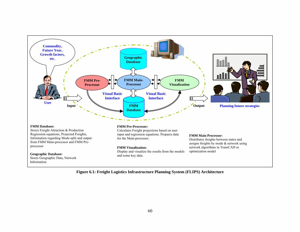
60

Geographic Database

FMM Database: Stores Freight Attraction & Production Regression equations, Projected Freights, Information regarding Mode-split and output from FMM Main-processor and FMM Pre-processor

User

FMM Pre-Processor

FMM Main- Processor

Commodity, Future Year,

Growth factors, etc.

Planning future strategies

Visual Basic Interface

FMM Visualization

Visual Basic Interface

FMM Database

Input Output

Geographic Database: Stores Geographic Data, Network Information

FMM Pre-Processor: Calculates Freight projections based on user input and regression equations. Prepares data for the Main-processor.

FMM Main Processor: Distributes freights between states and assigns freights by mode & network using network algorithms in TransCAD or optimization model

FMM Visualization: Display and visualize the results from the models and some key data.

Figure 6.1: Freight Logistics Infrastructure Planning System (FLIPS) Architecture

61

The calibration of the doubly constrained gravity model is critical for freight assignment which is achieved using the base year’s freight distribution matrix (O-D matrix). This process of calibration is done by TransCad® in the FMM Main-processor. The freight assignment also requires mode-split percentages for splitting the commodity flow between OD pairs to obtain the flow volume by a particular mode of transportation – highway, railway or waterway. The FMM pre-processor also allows the user to view and edit the freight attraction/production regression co-efficients and variable values. This demonstrates the adaptability and extensibility of the software in the sense that the user is provided with the capability of changing these values as and when new socioeconomic data e.g. population and employment data are available.

6.1.2 FMM Main-Processor The key task of the Main-processor is to assign commodity flow onto the network for each transport mode. The assignment can be implemented using the flow assignment module in TransCad®. The module provides many assignment algorithms, e.g., all-or-nothing, user equilibrium, system optimal and stochastic user equilibrium (discussed in Section 2.1.4). An initial version of an alternative way for the network assignment using simplified piecewise linear travel-time function has also been developed and implemented using Xpress Optimization software. The optimization model and the issues that need to be dealt with are presented in Appendix D. In case the future-year production and attraction flows are projected by the regression model, the Main-Processor is also used for freight distribution to obtain the OD freight matrix.

6.1.3 FMM Database This database stores all input and output data from the FMM Pre-processor, FMM Main-processor and FMM Visualization modules. Examples of input data include the population and employment numbers for the base year and the future years, commodity flows from FAF2, coefficients of regression models for production and attraction flows and the utilization ratio for the mode split model. Output data stored in the FMM database include the projected commodity flow and the mode-split flow from the Pre-processor and the OD freight matrix from the Main-processor.

6.1.4 FMM Geographic Database This component of the software stores geographical input and output data for other modules. The main geographical input data is the network structure for each transport mode. For the output, the geographical database stores the assignment results from the Main-processor, and data formatted for use by the FMM visualization module.

6.1.5 FMM Visualization The main purpose of this module is to visualize key data and the flow assignment results produced by the Main-processor. This module has been developed in-house using Visual Basic.Net and MapWindow GIS, which is open-source GIS software. Users who just want to look at some input data and the flow assignment results can use this module independently without interacting with other modules. The main page of this visualization tool, shown in Figure 6.2, has three menu tabs – one for file operations, one for analysis applications and the third for help.

62

Figure 6.2: Data Visualization Tool

The analysis applications of the data visualization module have three main parts – Summary of freight flow analysis and data, Basic queries and Advanced queries. The help menu consists of a user guide. The following sections discuss the various analysis applications.

6.1.5.1 Summary of Freight Flow Analysis This part of the FMM visualization provides freight flow analysis results for each mode in each year, critical path analysis for the highway network, production/attraction flow, population/ employment data, top commodities and top trading partners all at the county level. The critical path in this module is identified by volume per capacity ratio, therefore, congested links are selected and an in-depth analysis of the flow on these critical links is conducted. Figure 6.3 presents the summary of freight flow analysis window. The various summaries that are provided in this section include the freight flow analysis results, the Production/Attraction Flow and Population/Employment Data at the County Level, the critical path analysis, top commodities at each county, top trading partners for each county, etc. Figure 6.4 presents the results of the freight flow analysis, while Figure 6.5 presents the production/attraction flow and the population/employment data at each county. The results of the critical path analysis is presented in Figure 6.5, while Figures 6.6 and 6.7 present the top commodities at each county and the top trading partners at each county.

63

Figure 6.3: Summary of Freight Flow Analysis

Figure 6.4: Results of Freight Flow Analysis

64

Figure 6.5: Summary of Critical Path Analysis: UE 2002 v/c ratio greater than or equal to 1

On the critical path 1, critical links are 52780, 52778, 53096, 177090, 53100, 53101, 53097, 51706, and 53103. The top 20 OD pairs contributing flows on the critical path 1 are as follows.

Origin OID Destina tion DID SumOfQUERY1Cleveland 139820 Oklahoma 139822 603244.63Canadian 139804 Oklahoma 139822 377922.69Pottawatomie 139826 Oklahoma 139822 250872.83Oklahoma 139822 Cleveland 139820 210583.59Oklahoma 139822 Logan 139842 162204.66Oklahoma 139822 Lincoln 139846 151018.13TX Dalla 139575 KS rem 139618 105631.94Grady 139802 Oklahoma 139822 98723.05Oklahoma 139822 Canadian 139804 89585.28McClain 139818 Oklahoma 139822 55306.76Oklahoma 139822 Tulsa 139890 49285.54Oklahoma 139822 Pottawatomie 139826 45875.8Oklahoma 139822 KS rem 139618 41720.42CA Los A 139541 IL rem 139642 40425.82TX Dalla 139575 Oklahoma 139822 39304.84Oklahoma 139822 Grady 139802 31949.21TX Dalla 139575 KS Kansa 139620 30865.2TX rem 139569 IL Chica 139648 30006.49TX rem 139569 Oklahoma 139822 25869.58Oklahoma 139822 Creek 139884 25194.09

Table 6.1: Top 20 OD pairs contributing Flows on the Critical Path 1

65

If we assume that all commodities have the same utility function and mostly depend on travel time, we can trace back to the type of commodities from each OD pair. For example, for OD pair: TX Dalla-KS rem, the flows are as follows;

Origin Destination Commodity Mode SumOf2002 PercentTX Dalla KS rem Base metals Truck 1064310 0.453677812TX Dalla KS rem Basic chemicals Truck 12320 0.005251581TX Dalla KS rem Chemical prods. Truck 46310 0.01974032TX Dalla KS rem Electronics Truck 25190 0.010737608TX Dalla KS rem Furniture Truck 19130 0.008154444TX Dalla KS rem Gasoline Truck 113220 0.048261692TX Dalla KS rem Machinery Truck 33780 0.014399222TX Dalla KS rem Misc. mfg. prods. Truck 44870 0.019126498TX Dalla KS rem Mixed freight Truck 104580 0.044578765TX Dalla KS rem Motorized vehicles Truck 22630 0.009646371TX Dalla KS rem Newsprint/paper Truck 26130 0.011138297TX Dalla KS rem Nonmetal min. prods. Truck 296320 0.126310764TX Dalla KS rem Other foodstuffs Truck 60240 0.025678187TX Dalla KS rem Paper articles Truck 87660 0.037366366TX Dalla KS rem Plastics/rubber Truck 23550 0.010038534TX Dalla KS rem Precision instruments Truck 3760 0.001602755TX Dalla KS rem Printed prods. Truck 12960 0.005524391TX Dalla KS rem Textiles/leather Truck 13750 0.00586114TX Dalla KS rem Transport equip. Truck 103440 0.044092823TX Dalla KS rem Unknown Truck 220 9.37782E-05TX Dalla KS rem Waste/scrap Truck 250 0.000106566TX Dalla KS rem Wood prods. Truck 231340 0.098612082

2345960 1T ota l Table 6.2: Commodity-wise Flow Split from Dallas, Texas to Remainder of Kansas

Therefore, we can estimate that about 45% of flow from TX Dalla to KS rem are Base Metal products.

66

Figure 6.6: Top Commodities at a County

Figure 6.7: Top Trading Partners for a County

67

6.1.5.2 Basic Queries Basic query provides a user the ability to perform simple queries. The three basic queries designed in this menu include the search by flow volume, search by descending order of flow volume, and the search by volume/capacity ratio. If the user wants to search for the links which have a total flow greater than a particular value, the search by flow volume is used. The search by descending order of flow volume is used when the user wants to look for the top few links, while the search by volume/capacity ratio is used when the user needs the links with the volume/capacity ratio greater than a critical value. The user interface of the basic query is shown in Figure 6.8. The user can select the mode of transportation, the year, and the type of query from the drop down box. The years that can be selected are 2002, 2010, 2015, 2020, 2025, 2030, and 2035. The modes that can be selected are highway, railway, and waterway. The types of query include the following – high volume links, top links or the volume capacity ratio.

Figure 6.8: Basic Query Window

On selecting the high flow volume query, the following window will appear. The user can enter the threshold flow volume as shown in Figure 6.9.

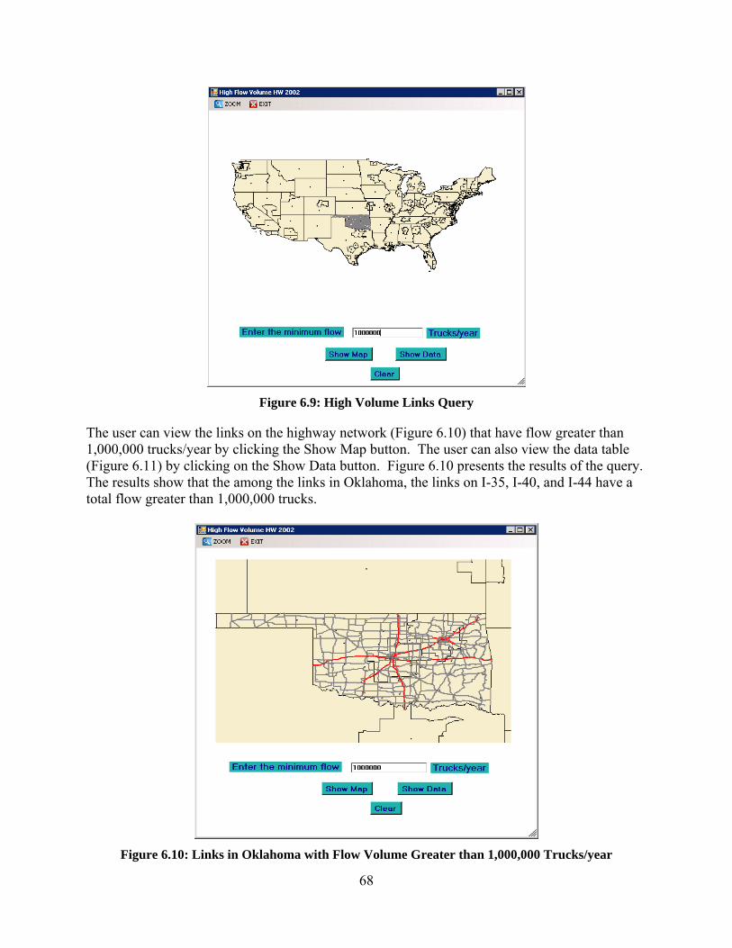
68

Figure 6.9: High Volume Links Query

The user can view the links on the highway network (Figure 6.10) that have flow greater than 1,000,000 trucks/year by clicking the Show Map button. The user can also view the data table (Figure 6.11) by clicking on the Show Data button. Figure 6.10 presents the results of the query. The results show that the among the links in Oklahoma, the links on I-35, I-40, and I-44 have a total flow greater than 1,000,000 trucks.

Figure 6.10: Links in Oklahoma with Flow Volume Greater than 1,000,000 Trucks/year

69

Figure 6.11: Data Table Containing Links with Flow Volume Greater than 1,000,000 Trucks/year

Similarly, the user can also search for the top 300 links as shown in Figure 6.12. As in the case of the high flow volume query, the user can use the Show Map and Show Data buttons to view the map (Figure 6.13) and data table, respectively. It can be seen that some of the links in I-35 and I-44 are among the top 300 links in Oklahoma.

Figure 6.12: Top Links Query

70

Figure 6.13: Top 300 Links in Oklahoma

Similarly, the user can also search for the links which have a volume/capacity ratio greater than 2.0 as shown in Figure 6.14. The result of the query is presented in Figure 6.15.

Figure 6.14: Volume/Capacity Ratio Query

71

Figure 6.15: Links in Oklahoma with Volume/Capacity Ratio >Greater than 2.0

6.1.5.3 Advanced Queries The advanced query menu in the FMM Visualization provides the capability for advanced search. In this menu, the query is performed directly through the MapWindow GIS application. All flow assignment results of all modes are stored in the MapWindow GIS application and users can utilize the advanced query tools available in the software to perform their own search. Figure 6.16 presents the screen shot of the Advanced Query.

Figure 6.16: Advanced Query Interface

72

7. SCENARIO ANALYSIS A key application of the FMM model and prototype is the support for performing “what-if” or scenario analysis. The research team has developed a few proof-of-concept scenarios that were analyzed using two different flow assignment algorithms – All-or-Nothing (AON) and User Equilibrium. The different scenarios that were explored include a bridge collapse scenario and an increase in population and employment in the counties of Oklahoma. The examples presented in the rest of this section should be considered as being representative of the scenario analysis that can be carried out with the FMM model. The results of the scenario analyses have not been validated and have been used to give the reader an idea into the potential insights that can be derived from them.

7.1 Bridge Collapse Scenario The motivation behind the bridge collapse scenario is the collapse of the I-40 bridge that occurred in Webber Falls, Oklahoma on May 26, 2002. This resulted in a reasonably large-scale rerouting of traffic. Such a scenario, where a critical link(s) in the transportation network is disabled because of manmade or natural disasters for an extended time period could help ODOT assess the readiness of nearby alternate thoroughfares to handle the increase in freight (and passenger) traffic because of re-routing.

7.1.1 Results from All-or-Nothing (AON) Assignment The AON assignment model assigns flows using the shortest path for each Origin and Destination (OD) pair. Consequently, the travel time is considered as directly related to distance and does not depend on the link volume, hence, ignores the fact that link travel time is related to link volume and capacity. In addition to that, even if there is another path with the same or close travel time or cost, only one path is used due to no consideration of link capacity. The number of trucks per day prior to the disaster and after the disaster are given in Figures 7.1 and 7.2 and Figures 7.3 and 7.4. When the two maps are compared, it is seen that the high volume traffic in pre-disaster flow was split into smaller flows.

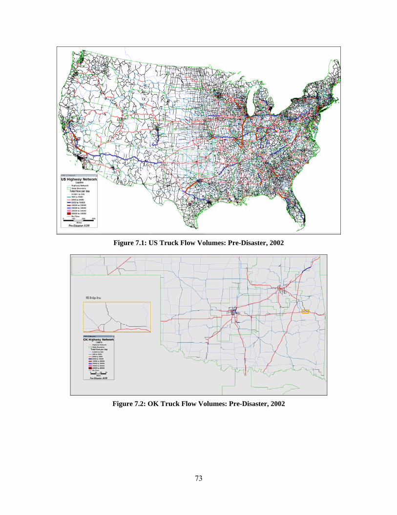
73

Figure 7.1: US Truck Flow Volumes: Pre-Disaster, 2002

Figure 7.2: OK Truck Flow Volumes: Pre-Disaster, 2002

74

Figure 7.3: US Truck Flow Volumes: Post-Disaster, 2002

Figure 7.4: OK Truck Flow Volumes: Post-Disaster, 2002

7.1.1.1 Pre-Disaster and Post-Disaster Assignment Comparison The AON assignment results of pre-disaster and post-disaster networks using the same set of O-D pairs and the freight in Number of Trucks (NT) are given in Table 7.1.

75

Performance Measures Pre disaster Post disaster Difference Change Total VHT 1,411,049,032 1,411,113,486 64,454 0.0046% Total VMT 84,662,941,912 84,666,809,167 3,867,254 0.0046%

Table 7.1: I-40 Bridge Collapse Pre-Post Comparison under AON

Using the comparison the following can be made with respect to the disaster: • Total Vehicle Hours Travelled (VHT) increased by 0.0046%, • Total Vehicle Miles Travelled (VMT) increased by 0.0046%.

Furthermore, the following insights can be obtained by analyzing the assignment results:

• 116,104 links continued to carry no flow. • Miles travelled increased 9.66 miles from pre-disaster to post-disaster network, which

corresponded to 0.006% increase in total miles travelled. • 7 links, which were not used in pre-disaster network, were used in post-disaster network

(Figure 7.5 – shown in blue). • 19 links used in pre-disaster network did not carry any flows in the post-disaster network

(Figure 7.5 – shown in yellow).

Figure 7.5: Link Usage Pre-Post Changes

• The highest increases and decreases occurred in the area surrounding the I40 Bridge (Figure 7.6).

• In total 4.49% of the links (7,692+bridge link of 171,171) had a different flow after the disaster. 2.92% of the links (5,000 of 171,171) had an increase whereas 1.57% of the links (2,693 of 171,171) had a decrease in number of trucks they carried. Changes in flows in US are given in Figure 7.5.

• 0.70% (1,192 of 171,171) of all links or 15.5% (1,192 of 7,693) of the links that had a change in freight flow are in the State of Oklahoma. This indicates that the bridge

76

collapse resulted more changes (84.5% of all changes) in other states’ transportation networks, rather than in the Oklahoma highway network. This means a local disaster can generate regional and national impact as well.

• Changes in US Transportation Network can be observed in Figure 7.7. The links in yellow to blue colors have a decrease in flow volume while those links in orange to red to purple colors have an increase in flow volume. This result indicates that a disaster like bridge collapse does not necessarily increase flows on all links. Also, links with flow changes (+ or -) are not necessarily nearby the disaster location, some links are closer, some are not, hence, no clear “distance delay” pattern as few existing publications indicated.

Figure 7.6: Post-Pre Disaster Difference I40 Bridge Area

77

Figure 7.7: Post-Pre Disaster Difference

7.1.2 Results from User Equilibrium (UE) Assignment In User Equilibrium Assignment (UE), the basic assumption is that no driver can unilaterally reduce his/her travel costs by shifting to another route. The deterministic user equilibrium is achieved by assuming that the drivers have perfect knowledge about travel costs on a network and so they choose the best route for themselves. UE makes use of attractive routes, and assigns a flow of zero to less attractive routes with a consideration of link capacities. Numbers of trucks per day prior to the disaster and after the disaster are given in Figure 7.8, 7.9, 7.10 and Figure 7.11.

78

Figure 7.8: US Truck Flow Volumes: Pre-Disaster, 2002

Figure 7.9: OK Truck Flow Volumes: Pre-Disaster, 2002

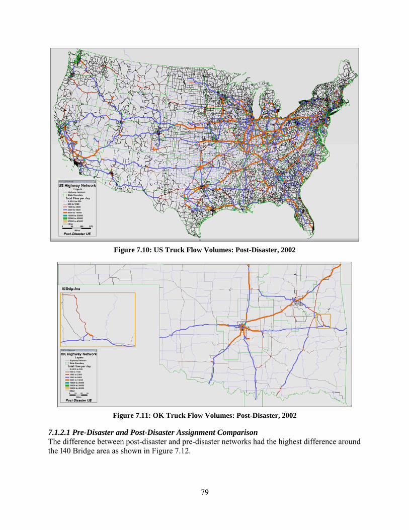
79

Figure 7.10: US Truck Flow Volumes: Post-Disaster, 2002

Figure 7.11: OK Truck Flow Volumes: Post-Disaster, 2002

7.1.2.1 Pre-Disaster and Post-Disaster Assignment Comparison The difference between post-disaster and pre-disaster networks had the highest difference around the I40 Bridge area as shown in Figure 7.12.

80

Figure 7.12: Post-Pre Disaster Difference in the I40 Bridge Area

Performance Measure Pre disaster Post disaster Post-Pre Change

Total VHT 30639976182 30639977124 942 0.0000031%Total VMT 88816750121 88820889731 4139609 0.0047%

Table 7.2: UE Performance Measures

From Table 7.2, it is seen that the disaster increased both Vehicle Miles Traveled (VMT) and Vehicle Hours Travelled (VHT), with much increase in VMT. In Figure 7.13, the difference in total flow is shown on the US highway network by colors. Again, the colors from yellow to blue show the links with a flow decrease, while the colors from orange to red to purple show a flow increase. Also, the flow changes (+/-) spread out in the United States and Oklahoma.

81

Figure 7.13: Post-Pre Disaster Difference

Analysis of assignment results showed the followings: • 154,092 miles (56,868 links of 171,172 links) had a different total flow after the disaster. • 7,974 miles (2,582 of the total links) having a change in total flow were in the Oklahoma

transportation network. We defined a weighted difference measure as the [length of the link*(difference in total flow)2], which considers not only the affected length of the network but also the change on the link.

• 179,886,438 (mile*NT2) change was experienced on US highway network • 171,736,024 (mile*NT2) change was experienced on Oklahoma highway network

5% (which is 81% of the total Oklahoma transportation network-miles) of all affected transportation network links are in Oklahoma and carry 95% (mile*NT2) of all changes, whereas the rest of the changes were on highways in other states. We can conclude that congestion experienced was higher in Oklahoma highways than others, while the effect was widely dispersed away from the bridge region.

82

Figure 7.14: Oklahoma Highway Network Weighted Difference

In Figure 7.14, the weighted difference on Oklahoma highway network is shown. In Figure 7.15, the weighted difference on US highway network is given. From this figure, the highest weighted changes were observed at the following states: OK, TX, CA, AR, KS, IL, IN, OH, and WI. This information suggests that due to the I40 Bridge collapse the listed states were affected the most, having an increased congestion on their highway networks. It is also clear that some links with most flow fluctuation are closer to the bridge, but some are far away from the bridge in other states, such as California, Texas, Illinois, Wisconsin, etc., indicating again a local event can have regional and national impact on freight flow.

Figure 7.15: US Highway Network Weighted Difference

83

7.2 Employment and Population Increase Scenario Oklahoma has a steady growth rate in employment and population. This scenario considered an increase of employment by 10,000 and 5,000 in OKC and Tulsa respectively. Due to the employment increase, population will increase as a result. The population increase was assumed to be twice as much the employment increase, 20,000 in OKC and 10,000 in Tulsa.

7.2.1 Methodology The state total employment by SCTG commodity for years 1998 to 2006 was calculated. Table 7.3 shows the total SCTG employment in Oklahoma. Using the data of the year’s 2003 to 2006 employment for the year 2010 was forecasted using a linear regression model (Figure 7.16).

1998 1999 2000 2001 2002 2003 2004 2005 2006Total SCTGEmployment 624228 624213 623967 624214 623920 623837 618827 623986 629037

Table 7.3: Oklahoma SCTG Total Employment

Figure 7.16: Oklahoma SCTG Employment Forecast

Year 2010 SCTG employment was forecasted to be 635,340. SCTG county employment is calculated for each county by using the total state forecast and county employment averages in previous years. At this step, changes in OKC and Tulsa were introduced. After the new employment totals for counties ratio within state and within MSA are calculated, 2010 MSA modified ratios were used to split FAF freight data from MSA level to county level for Oklahoma (Table 7.4). In the same manner 2010 population was forecasted using the same county ratios as those used in the combined regional-state model splits. OKC and Tulsa populations were increased by 20,000 and 10,000 and modified ratios at MSA level were calculated (Table 7.5).

84

ID County Names

MSA Average Ratio

2010 Emp

2010 Modified

Emp

2010 Modified

Ratio

2010 Modified Ratio by

MSA 1 Adair OK Rem 0.0056 3556 3556 0.0055 0.0156 3 Alfalfa OK Rem 0.0009 552 552 0.0008 0.0024 5 Atoka OK Rem 0.0024 1540 1540 0.0024 0.0067 7 Beaver OK Rem 0.0010 647 647 0.0010 0.0028 9 Beckham OK Rem 0.0061 3869 3869 0.0059 0.0169

11 Blaine OK Rem 0.0029 1823 1823 0.0028 0.0080 13 Bryan OK Rem 0.0105 6649 6649 0.0102 0.0291 15 Caddo OK Rem 0.0037 2352 2352 0.0036 0.0103 17 Canadian OK Okla 0.0202 12803 12803 0.0197 0.0550 19 Carter OK Rem 0.0147 9339 9339 0.0144 0.0409 21 Cherokee OK Rem 0.0062 3922 3922 0.0060 0.0172 23 Choctaw OK Rem 0.0028 1793 1793 0.0028 0.0079 25 Cimarron OK Rem 0.0009 546 546 0.0008 0.0024 27 Cleveland OK Okla 0.0390 24786 24786 0.0381 0.1065 29 Coal OK Rem 0.0009 571 571 0.0009 0.0025 31 Comanche OK Rem 0.0258 16380 16380 0.0252 0.0717 33 Cotton OK Rem 0.0007 422 422 0.0006 0.0018 35 Craig OK Rem 0.0050 3195 3195 0.0049 0.0140 37 Creek OK Tulsa 0.0151 9611 9611 0.0148 0.0508 39 Custer OK Rem 0.0098 6202 6202 0.0095 0.0272 41 Delaware OK Rem 0.0062 3945 3945 0.0061 0.0173 43 Dewey OK Rem 0.0013 818 818 0.0013 0.0036 45 Ellis OK Rem 0.0010 638 638 0.0010 0.0028 47 Garfield OK Rem 0.0230 14642 14642 0.0225 0.0641 49 Garvin OK Rem 0.0070 4421 4421 0.0068 0.0194 51 Grady OK Okla 0.0106 6765 6765 0.0104 0.0291 53 Grant OK Rem 0.0010 656 656 0.0010 0.0029 55 Greer OK Rem 0.0010 644 644 0.0010 0.0028 57 Harmon OK Rem 0.0006 353 353 0.0005 0.0015 59 Harper OK Rem 0.0008 512 512 0.0008 0.0022 61 Haskell OK Rem 0.0022 1408 1408 0.0022 0.0062 63 Hughes OK Rem 0.0023 1475 1475 0.0023 0.0065 65 Jackson OK Rem 0.0092 5874 5874 0.0090 0.0257 67 Jefferson OK Rem 0.0011 708 708 0.0011 0.0031 69 Johnston OK Rem 0.0038 2427 2427 0.0037 0.0106 71 Kay OK Rem 0.0169 10742 10742 0.0165 0.0470 73 Kingfisher OK Rem 0.0054 3434 3434 0.0053 0.0150 75 Kiowa OK Rem 0.0025 1583 1583 0.0024 0.0069 77 Latimer OK Rem 0.0016 1019 1019 0.0016 0.0045

85

79 Le Flore OK Rem 0.0083 5250 5250 0.0081 0.0230 81 Lincoln OK Okla 0.0041 2630 2630 0.0040 0.0113 83 Logan OK Okla 0.0041 2603 2603 0.0040 0.0112 85 Love OK Rem 0.0024 1495 1495 0.0023 0.0065 93 Major OK Rem 0.0021 1355 1355 0.0021 0.0059 95 Marshall OK Rem 0.0050 3159 3159 0.0049 0.0138 97 Mayes OK Rem 0.0113 7158 7158 0.0110 0.0314 87 McClain OK Okla 0.0053 3353 3353 0.0052 0.0144 89 McCurtain OK Rem 0.0137 8726 8726 0.0134 0.0382 91 McIntosh OK Rem 0.0031 1949 1949 0.0030 0.0085 99 Murray OK Rem 0.0034 2164 2164 0.0033 0.0095 101 Muskogee OK Rem 0.0199 12625 12625 0.0194 0.0553 103 Noble OK Rem 0.0019 1195 1195 0.0018 0.0052 105 Nowata OK Rem 0.0015 935 935 0.0014 0.0041 107 Okfuskee OK Rem 0.0019 1196 1196 0.0018 0.0052 109 Oklahoma OK Okla 0.2504 159091 169091 0.2600 0.7264 111 Okmulgee OK Tulsa 0.0068 4296 4296 0.0066 0.0227 113 Osage OK Tulsa 0.0042 2690 2690 0.0041 0.0142 115 Ottawa OK Rem 0.0073 4626 4626 0.0071 0.0203 117 Pawnee OK Tulsa 0.0030 1891 1891 0.0029 0.0100 119 Payne OK Rem 0.0187 11850 11850 0.0182 0.0519 121 Pittsburg OK Rem 0.0092 5828 5828 0.0090 0.0255 123 Pontotoc OK Rem 0.0117 7446 7446 0.0114 0.0326 125 Pottawatomie OK Okla 0.0169 10753 10753 0.0165 0.0462 127 Pushmataha OK Rem 0.0021 1341 1341 0.0021 0.0059 129 Roger Mills OK Rem 0.0006 409 409 0.0006 0.0018 131 Rogers OK Tulsa 0.0181 11480 11480 0.0177 0.0607 133 Seminole OK Rem 0.0058 3716 3716 0.0057 0.0163 135 Sequoyah OK Rem 0.0055 3495 3495 0.0054 0.0153 137 Stephens OK Rem 0.0108 6836 6836 0.0105 0.0299 139 Texas OK Rem 0.0139 8845 8845 0.0136 0.0387 141 Tillman OK Rem 0.0020 1254 1254 0.0019 0.0055 143 Tulsa OK Tulsa 0.2252 143073 148073 0.2277 0.7825 145 Wagoner OK Tulsa 0.0062 3961 3961 0.0061 0.0209 147 Washington OK Tulsa 0.0114 7231 7231 0.0111 0.0382 149 Washita OK Rem 0.0016 1021 1021 0.0016 0.0045 151 Woods OK Rem 0.0025 1602 1602 0.0025 0.0070 153 Woodward OK Rem 0.0066 4189 4189 0.0064 0.0183

Total 635339 650339

Table 7.4: Oklahoma Employment Projections

86

CountyID MSA County Name 2010Population 2010 Modified Population

2010 Ratio 2010 Modified Ratio by MSA

1 OK Rem Adair 21350 21350 0.0059 0.0155 3 OK Rem Alfalfa 5080 5080 0.0014 0.0037 5 OK Rem Atoka 14180 14180 0.0039 0.0103 7 OK Rem Beaver 4842 4842 0.0013 0.0035 9 OK Rem Beckham 20726 20726 0.0057 0.0150

11 OK Rem Blaine 12032 12032 0.0033 0.0087 13 OK Rem Bryan 39081 39081 0.0108 0.0284 15 OK Rem Caddo 28623 28623 0.0079 0.0208 17 OK Okla Canadian 106055 106055 0.0293 0.0829 19 OK Rem Carter 46830 46830 0.0129 0.0340 21 OK Rem Cherokee 43891 43891 0.0121 0.0319 23 OK Rem Choctaw 14481 14481 0.0040 0.0105 25 OK Rem Cimarron 2430 2430 0.0007 0.0018 27 OK Okla Cleveland 237769 237769 0.0657 0.1858 29 OK Rem Coal 5487 5487 0.0015 0.0040 31 OK Rem Comanche 111877 111877 0.0309 0.0812 33 OK Rem Cotton 6141 6141 0.0017 0.0045 35 OK Rem Craig 14651 14651 0.0040 0.0106 37 OK Tulsa Creek 69422 69422 0.0192 0.0720 39 OK Rem Custer 25568 25568 0.0071 0.0186 41 OK Rem Delaware 38886 38886 0.0107 0.0282 43 OK Rem Dewey 4257 4257 0.0012 0.0031 45 OK Rem Ellis 3698 3698 0.0010 0.0027 47 OK Rem Garfield 57460 57460 0.0159 0.0417 49 OK Rem Garvin 28204 28204 0.0078 0.0205 51 OK Okla Grady 49876 49876 0.0138 0.0390 53 OK Rem Grant 4618 4618 0.0013 0.0034 55 OK Rem Greer 5639 5639 0.0016 0.0041 57 OK Rem Harmon 2572 2572 0.0007 0.0019 59 OK Rem Harper 3209 3209 0.0009 0.0023 61 OK Rem Haskell 12029 12029 0.0033 0.0087 63 OK Rem Hughes 13218 13218 0.0036 0.0096 65 OK Rem Jackson 24228 24228 0.0067 0.0176 67 OK Rem Jefferson 5830 5830 0.0016 0.0042 69 OK Rem Johnston 10316 10316 0.0028 0.0075 71 OK Rem Kay 42605 42605 0.0118 0.0309 73 OK Rem Kingfisher 13787 13787 0.0038 0.0100 75 OK Rem Kiowa 9028 9028 0.0025 0.0066 77 OK Rem Latimer 10367 10367 0.0029 0.0075 79 OK Rem Le Flore 48091 48091 0.0133 0.0349

87

81 OK Okla Lincoln 31432 31432 0.0087 0.0246 83 OK Okla Logan 36241 36241 0.0100 0.0283 85 OK Rem Love 9166 9166 0.0025 0.0067 93 OK Rem Major 6860 6860 0.0019 0.0050 95 OK Rem Marshall 14980 14980 0.0041 0.0109 97 OK Rem Mayes 38367 38367 0.0106 0.0279 87 OK Okla McClain 32009 32009 0.0088 0.0250 89 OK Rem McCurtain 32347 32347 0.0089 0.0235 91 OK Rem McIntosh 19394 19394 0.0054 0.0141 99 OK Rem Murray 12372 12372 0.0034 0.0090 101 OK Rem Muskogee 71121 71121 0.0196 0.0516 103 OK Rem Noble 10744 10744 0.0030 0.0078 105 OK Rem Nowata 10432 10432 0.0029 0.0076 107 OK Rem Okfuskee 10678 10678 0.0029 0.0078 109 OK Okla Oklahoma 696997 716997 0.1980 0.5603 111 OK Tulsa Okmulgee 38889 38889 0.0107 0.0403 113 OK Tulsa Osage 45018 45018 0.0124 0.0467 115 OK Rem Ottawa 32104 32104 0.0089 0.0233 117 OK Tulsa Pawnee 15846 15846 0.0044 0.0164 119 OK Rem Payne 83772 83772 0.0231 0.0608 121 OK Rem Pittsburg 43213 43213 0.0119 0.0314 123 OK Rem Pontotoc 36673 36673 0.0101 0.0266 125 OK Okla Pottawatomie 69325 69325 0.0191 0.0542 127 OK Rem Pushmataha 11521 11521 0.0032 0.0084 129 OK Rem Roger Mills 3196 3196 0.0009 0.0023 131 OK Tulsa Rogers 85630 85630 0.0236 0.0888 133 OK Rem Seminole 23252 23252 0.0064 0.0169 135 OK Rem Sequoyah 41614 41614 0.0115 0.0302 137 OK Rem Stephens 43800 43800 0.0121 0.0318 139 OK Rem Texas 19961 19961 0.0055 0.0145 141 OK Rem Tillman 7628 7628 0.0021 0.0055 143 OK Tulsa Tulsa 583254 593254 0.1638 0.6151 145 OK Tulsa Wagoner 66995 66995 0.0185 0.0695 147 OK Tulsa Washington 49451 49451 0.0137 0.0513 149 OK Rem Washita 11981 11981 0.0033 0.0087 151 OK Rem Woods 7654 7654 0.0021 0.0056 153 OK Rem Woodward 19163 19163 0.0053 0.0139

Total 3591516 3621516

Table 7.5: Oklahoma Population Modification

88

We defined a weighted difference measure as the [length of the link*(difference in total flow)2], which considers not only the affected length of the network but also the change on the link.

7.2.2 Results and Analysis Under All-or-Nothing (AON) Assignment

Figure 7.17: 2002 USA AON Weighted Difference: Prior-After Employment-Population Increase

Figure 7.18: 2002 Oklahoma AON Weighted Difference: Prior-After Employment-Population

Increase

89

Figures 7.17 and 7.18 show that employment and population increases in OKC and Tulsa caused positive (increase) highway freight flow changes on some links. The largest flow increases occur in Oklahoma and nearby regions, indicating strong local and regional impact. However, some links far away Oklahoma do have some flow increases.

7.2.3 Results and Analysis Under User Equilibrium (UE) Assignment

Figure 7.19: 2010 USA UE Weighted Difference: Prior-After Employment-Population Increase

Figure 7.20: 2010 Oklahoma UE Weighted Difference: Prior-After Employment-Population

Increase

90

Under User Equilibrium (UE) assignments, employment and population increases in OKC and Tulsa also generated weighted flow increase. Figure 7.19 shows that the changes are on links which are mostly in Oklahoma and surrounding areas. Figure 7.20 is a close-up view of link flow changes in Oklahoma. Figures 7.19 and 7.20 show more links have flow changes than Figures 7.17 and 7.18, indicating the fundamental difference of AON and UE is the capacity impact under UE assignments.

91

8. FUTURE RESEARCH

The problem of forecasting freight movement into the future is a complex combination of data management, demand and supply forecasting, and modeling the distribution of freight flow. In addition, the difficult task of developing software is necessary to support each of these areas. Each of these areas taken by itself is a difficult research area. However, over the last 6 years, the Freight Movement Model for the State of Oklahoma (FMM) project has tackled each of these problems and has successfully developed a software prototype that addresses data management, forecasting, and modeling the distribution of freight flow. This work has laid the groundwork for two primary areas of research, which are being pursued as part of an on-going joint OSU/OU project funded by the OTC. The primary goals of this on-going project are as follows. 1. Design and develop a decision support software environment that can support critical decisions related to transportation infrastructure planning in the public sector and supply chain system planning in the private sector. 2. Extend the FMM methodology developed by the research team for freight movement modeling to supply chain system planning problems pertaining to the logistical infrastructure.

92

REFERENCES

1. Oklahoma Department of Transportation, “2000-2025 Statewide Intermodal Transportation Plan”, Oklahoma Transportation Commission, 2001.

2. Cambridge Systematics, Inc., NCHRP Report 388: “A Guidebook for Forecasting Freight Transportation Demand”, Transportation Research Board, Washington D.C., 1997.

3. Cambridge Systematics, Inc., Comsis Corportation and University of Wisconsin, Milwaukee, “Quick Response Freight Manual Final Report”, U.S. Department of Transportation, Washington, D.C., 1996. Retrieved from http://tmip.fhwa.dot.gov/clearinghouse/docs/quick/ on June 2002.

4. Center for Urban Transportation Studies, University of Wisconsin, Milwaukee, “Guidebook on Statewide Travel Forecasting”, 1999. Retrieved from http://www.fhwa.dot.gov/hep10/state/swtravel.pdf on June 2002

5. U.S. Census Bureau Homepage, “1997 Economic Census Data”, Retrieved from http://www.census.gov/epcd/www/econ97.html on June 2002

6. U.S. Census Bureau, “Economic Report Series 1997”, CD ROM, U.S. Census Bureau, 2001 7. Black, W. R., “Transport Flows in the State of Indiana: Commodity Database Development and

Traffic Assignment Phase 2”, Transportation Research Center, Indiana University, Bloomington, 1997.

8. Wilbur Smith Associates, “Multimodal Freight Forecasts for Wisconsin”, Wisconsin Department of Transportation, 1996.

9. Bureau of Transportation Statistics, “Commodity Flow Survey”, Retrieved from http://www.bts.gov/publications/commodity_flow_survey/ on July 2008.

10. Bureau of Transportation Statistics, “National Transportation Atlas Database”, Retrieved from http://www.bts.gov/publications/national_transportation_atlas_database/2006/ on July 2008.

11. C. Ojha, “Comparison of Freight Flows on US Highway Network Using GIS and Optimal Flow Assigments,” M.S. Thesis, Department of Industrial Engineering, University of Oklahoma, Norman, OK., 2008.

12. Cambridge Systematics Inc., Reebie Associates, Inc. and Mid-Ohio Regional Planning Commission, “Final Report Freight Impact on Ohio’s Roadways,” pp 1-1 to 1-8, 2002, from http://www.dot.state.oh.us/research/2002/Planning/14766-FR.pdf, Retrieved Jan 28, 2008.

13. Federal Highway Administration, “Freight Analysis Framework,” Washington, D.C., 2002, from http://ops.fhwa.dot.gov/freight/freight_analysis/faf/index.htm, Retrieved Dec 1, 2007.

14. Bingham, P., Forecast Summary: Commodity Flow Forecast Update and Lower Columbia River Cargo Forecast. DRI-WEFA Inc. pp 80, 2002, from http://www.flypdx.com/PDFPOP/Trade_Trans_Studies_LCR_Cmdty_Flw_Rpt.pdf, Retrieved January 28, 2008.

15. N. Oppenheim, Urban Travel Demand Modeling – From Individual Choices to General Equilibrium, Wiley-Interscience, New York, 1994.

16. Beckmann, M., C. B. McGuire & C. B. Winston. “Studies in the Economics of Transportation,” Yale University Press, New Haven, CT, 1956.

17. Bar-Gera, H., “Origin-based Algorithm for the Traffic Assignment Problem,” Transportation Science. Vol. 36, Issue 4 pp 398-418, 2002.

18. Mathew, T. V., “Transportation Network Design,” 2006, from http://www.civil.iitb.ac.in/~vmtom/1-cwt/14-ce744/72-tassignment/tassignment/tassignment.html, Retrieved February 25, 2008.

19. Prashker, J.N. & Bekhor, S., “Congestion, stochastic and similarity effects in stochastic user equilibrium models,” Transportation Research Record, 1733, pp.80-87, 2000.

20. Daganzo, C.F. & Sheffi, Y., “On stochastic models of traffic assignment,” Transportation Science, 253-274, 1977.

93

21. Sheffi, Y. & Powell, W. B., “An Algorithm for the Equilibrium Assignment Problem with Random Link Times,” Networks 12, 2, pp 191-207, 1982.

22. Taplin, J., “Simulation models of traffic flow,” Department of Information Management and Marketing, University of Western Australia, 1999, from http://www.orsnz.org.nz/conf34/PDFs/Taplin.pdf, Retrieved April 26, 2008.

23. Jayakrishnan, R. Tsai, Wei K., Prashker, J. N. & Rajadhyaksha, S., “A Faster path based algorithm for traffic assignment,” Transportation Research Record 1443. pp 75-81, 1994.

24. MapWindow GIS, 2006, from http://www.mapwindow.com/, retrieved Feb 19, 2009. 25. Standard Classification of Transported Goods: Definitions, Data Sources and Methods, from

http://www.statcan.ca/english/Subjects/Standard/sctg/sctg-intro.htm, retrieved October 20, 2007. 26. Furness, K.P., “Time Function Interaction”, Traffic Engineering and Control, 7(1971), 19-36. 27. Evans, S. P., "A Relationship between the Gravity Model for Trip Distribution and the

Transportation Problem in Linear Programming", Transportation Research, 7 (1973), 39-61. 28. Evans, S.P., "Derivation and Analysis of Some Models for Combining Trip Distribution and

Assignment." Transportation Research, 10(1976), 37-57. 29. Evans, S. P., and Kirby, H. R., “A Three-Dimensional Furness Procedure for Calibrating Gravity

Models.” Transportation Research 8 (1974), 105-122. 30. Brogan, J. J., Brich, S.C., and Demetsky, M. J., “Application of Statewide Intermodal Freight

Planning Methodology – Final Report”, (2001),Virginia Transportation Research Council, VA 31. LeBeau, L. "Planning For Grain Movement By Railroad and Truck in The United States: An

Exploratory Analysis of Mode-Split Factors for Freight Transportation", M.S. Thesis, Department of Industrial Engineering, University of Oklahoma, Norman, OK., 2007.

32. Bureau of Public Roads, “Traffic Assignment Manual”, Urban Planning Division, U.S. Department of Commerce, Washington DC, U.S., (1964).

33. Ortuzar, J. D. and Willumsen, L. G., “Modelling Transport”, John Wiley & Sons, Chichester, West Sussex, England, (1990).

94

APPENDIX A: DATA SOURCES AND INPUT PARAMETERS The following table shows the grouping of the 43 commodity types into three major categories – consumer goods, industrial commodities, and industry/consumer goods [25].

SCTG Code

Commodity Description

Consumer goods 5 Meat, fish, seafood, and their preparations 6 Milled grain products and preparations, and bakery products 7 Other prepared foodstuffs and fats and oils 8 Alcoholic beverages 9 Tobacco products 21 Pharmaceutical products 28 Paper or paperboard articles 29 Printed products 39 Furniture, mattresses and supports, lamps, lighting fittings, and illuminated

signs 40 Miscellaneous manufactured products Industrial goods 1 Live animals and live fish 10 Monumental or building stone 11 Natural sands 12 Gravel and crushed stone 13 Nonmetallic minerals, n.e.c. 14 Metallic ores and concentrates 15 Coal 17 Gasoline and aviation turbine fuel 18 Fuel oils 20 Basic chemicals 25 Logs and other wood in the rough 27 Pulp, newsprint, paper, and paperboard 32 Base metal in primary or semi-finished forms and in finished basic shapes 34 Machinery 37 Transportation equipment, n.e.c. 41 Waste and scrap 43 Mixed freight Both industry and consumer goods 2 Cereal grains 3 Other agricultural products 4 Animal feed and products of animal origin, n.e.c. 19 Coal and petroleum products, n.e.c. 22 Fertilizers 23 Chemical products and preparations, n.e.c. 24 Plastics and rubber

95

26 Wood products 30 Textiles, leather, and articles of textiles or leather 31 Nonmetallic mineral products 33 Articles of base metal 35 Electronic and other electrical equipment and components, and office

equipment 36 Motorized and other vehicles (including parts) 38 Precision instruments and apparatus

Table A.1: Commodity categorization based on end user

The following table shows data excluded from 1997 Economic census cover in CBP and that will be included in 2002 [5].

NAICS

Industry category excluded from the 1997 Economic Census

Included in 2002 Census

Coverage in CBP

11 Agriculture, Forestry, Fishing and Hunting

CBP (except 111, 112)

481111 Scheduled Passenger Air Transportation (part)

CBP

482 Rail Transportation 491 Postal Service 5251 Insurance and Employee Benefit

Funds

52591 Open-End Investment Funds CBP 52592 Trusts, Estates, and Agency

Accounts

52599 Other Financial Vehicles CBP 54132 Landscape Architectural Services 2002 CBP 54194 Veterinary Services 2002 CBP 56173 Landscaping Services 2002 CBP 6111 Elementary and Secondary

Schools CBP

6112 Junior Colleges CBP 6113 Colleges, Universities, and

Professional Schools CBP

81291 Pet Care (except Veterinary Services)

2002 CBP

8131 Religious Organizations CBP 81393 Labor Unions and Similar Labor

Organizations CBP

81394 Political Organizations CBP 814 Private Households 92 Public Administration

Table A.2: Data exclusions from the 1997 Economic Census

96

The summary of results of code mapping for each of the forty two commodity types are presented in Table A.3.

SCTG Code

Commodity Type Commodity Constituents Mapped NAICS Industry

01 Live animals and live fish Live animals, live fish, poultry, bovine animals, Swine

***

02 Cereal grains Wheat, corn, barley, oats etc 42251 03 Other agricultural products Fresh vegetables, chilled

vegetables, fruits & nuts, other agricultural products like soy bean, cotton etc

42291

04 Animal feed and products of animal origin

Straw/husk, inedible flour, dog & cat food, raw hide, skin, eggs etc

3111

05 Meat, fish, seafood and their preparations

Fresh meat/fish/poultry, chilled meat/fish/poultry, frozen meat/fish/poultry, extracts and juices of fish/meat

3116, 3117

06 Milled grain products, preparations and bakery products

Milled grain products: malt, wheat, rice, flour etc. Bakery products: dough, snack food, pastries

3118, 31121

07 Other prepared food stuff, fats and oil

Dairy products: milk, cheese, curd, butter etc Processed food: frozen vegetables, chips, juice etc Coffee, tea, spices, Sugar, Cocoa preparation, Non-alcoholic beverages etc

3113, 3114, 3115, 31122, 31192, 31194

08 Alcoholic beverages Beer, wine, liquor, spirits etc 4228, 31212, 31213, 31214

09 Tobacco products Cigarettes and miscellaneous tobacco products

3122, 42294

10 Monumental and building stones

11 Natural sand Silica sands, quartz sands, sand for industrial purpose and sand for construction purpose

21232, 42132

12 Gravel and crushed stones Crushed/broken lime stone, other crushed stones etc

21231

13 Non-metallic minerals n.e.c Table salt, phosphates, sulphur, clay, gypsum.

***

14 Metallic ores and concentrates

Iron, copper, nickel, lead, aluminum and zinc ores

***

15 Coal Types of coal: bituminous, 2121

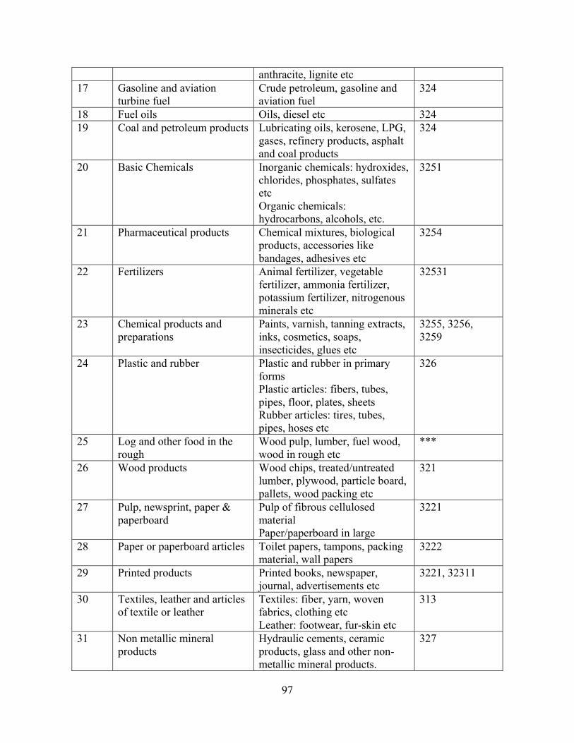
97

anthracite, lignite etc 17 Gasoline and aviation

turbine fuel Crude petroleum, gasoline and aviation fuel

324

18 Fuel oils Oils, diesel etc 324 19 Coal and petroleum products Lubricating oils, kerosene, LPG,

gases, refinery products, asphalt and coal products

324

20 Basic Chemicals Inorganic chemicals: hydroxides, chlorides, phosphates, sulfates etc Organic chemicals: hydrocarbons, alcohols, etc.

3251

21 Pharmaceutical products Chemical mixtures, biological products, accessories like bandages, adhesives etc

3254

22 Fertilizers Animal fertilizer, vegetable fertilizer, ammonia fertilizer, potassium fertilizer, nitrogenous minerals etc

32531

23 Chemical products and preparations

Paints, varnish, tanning extracts, inks, cosmetics, soaps, insecticides, glues etc

3255, 3256, 3259

24 Plastic and rubber Plastic and rubber in primary forms Plastic articles: fibers, tubes, pipes, floor, plates, sheets Rubber articles: tires, tubes, pipes, hoses etc

326

25 Log and other food in the rough

Wood pulp, lumber, fuel wood, wood in rough etc

***

26 Wood products Wood chips, treated/untreated lumber, plywood, particle board, pallets, wood packing etc

321

27 Pulp, newsprint, paper & paperboard

Pulp of fibrous cellulosed material Paper/paperboard in large

3221

28 Paper or paperboard articles Toilet papers, tampons, packing material, wall papers

3222

29 Printed products Printed books, newspaper, journal, advertisements etc

3221, 32311

30 Textiles, leather and articles of textile or leather

Textiles: fiber, yarn, woven fabrics, clothing etc Leather: footwear, fur-skin etc

313

31 Non metallic mineral products

Hydraulic cements, ceramic products, glass and other non-metallic mineral products.

327

98

32 Base metal in primary or semi-finished forms

Sheets, rolls, wires, bars, angle, shape and unwrought forms of metal etc

331

33 Articles of base metal Pipes, tubes, fittings, cutleries, hand tools etc Structures: doors, windows etc

332

34 Machinery IC engine, turbine, boiler, propeller, pump, refrigeration system, agriculture equipment etc

333

35 Motorized and other vehicles (including parts)

Vehicles: automobiles, tractors, bicycles, truck etc Parts: brakes, gear box, wheel, seating etc

3363

37 Transportation equipment Railway: locomotives, rolling stock, fittings etc Aircraft equipments Ships: boats, floating structures etc

3364, 3365, 3366

38 Precision instrument and apparatus

Eyewear, optical element, surgical/medical equipments, photocopying equipment, surveying tools etc

3391

39 Furniture, mattresses and lightings

Furniture: indoor and outdoor Lightings: all types of lighting accessories and fittings

337

40 Miscellaneous manufactured products

Arms, ammunition, jeweler, writing/drawing instruments, precious metals, antiques etc

3399

41 Waste and scrap Metallic waste, non-metallic waste and other miscellaneous waste items

3222, 327, 331

42 Mixed freight Office supplies, hardware, plumbing supplies, groceries, convenience store supplies etc.

311, 4217, 33994

NOTE: *** in the column of mapped industry implies: satisfactory results not obtained yet. Table A.3: Summary of the code mapping results

99

APPENDIX B: REGIONAL FREIGHT MOVEMENT MODEL The regional freight movement model is based on the four-step freight demand model, which has been adapted from the traditional Urban Travel Demand Model. The Urban Travel Demand Model has 4-steps to forecast passenger demand, namely freight generation, freight distribution, mode choice and freight assignment [15]. The inputs to this model are the socio-economic data at the state/MSA level. The regional model development has the following three steps.

• Freight generation (freight production and freight attraction) using regression models • Freight distribution using a gravity model or a mathematical programming model • Mode split using historical mode choice data • Freight assignment using a transportation network model

B.1 Freight Generation Freight generation is the first step undertaken in the traditional four-step urban travel demand modeling (UTDM). The objective of freight generation is to determine the tonnage that is produced at an origin and consumed at a destination. This step has two phases – the freight production phase and the freight attraction phase.

B.1.1 Freight Production The objective of freight production is to evaluate the tonnage of freight that originates at each origin location. A freight origination is a result of the production of that particular commodity type by the corresponding industry or organizations. Hence, a preceding task to freight production is to establish the aforementioned correspondence between industry and commodity type. The FMM project refers to the process of associating each of the commodity types to its corresponding set of producing/affecting industries as code mapping (discussed in detailed in Section 3.2.3). On accomplishing the code mapping, the subsequent task is to identify the appropriate parameters that reflect the growth of the concerned set of industries. The current section includes:

• Freight production (mathematical model) • Databases • Regression methodology

B.1.1.1 Freight Production – Mathematical Model Freight production employs a regression-based methodology with freight production/tonnage as the dependent variable and the various combinations of industry and socio-economic parameters as independent variables. The regression analysis evaluates a set of intercept, coefficients and error for each commodity type. Hence, the forecasting equation based on socio economic and industry variables is obtained and can be used to evaluate freight production in future years. The mathematical formulation of the freight production model is as shown below: -

Production = function {socio-economic factors, industry parameters}

nl

inlnlnin XAAP ε++= ∑ ]*[

where i = index of origin, n = commodities, l = independent variable

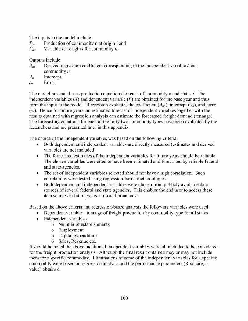
100

The inputs to the model include Pin Production of commodity n at origin i and Xinl Variable l at origin i for commodity n. Outputs include An1 Derived regression coefficient corresponding to the independent variable l and

commodity n, An Intercept, εn Error. The model presented uses production equations for each of commodity n and states i. The independent variables (X) and dependent variable (P) are obtained for the base year and thus form the input to the model. Regression evaluates the coefficient (Anl ), intercept (An), and error (εn). Hence for future years, an estimated forecast of independent variables together with the results obtained with regression analysis can estimate the forecasted freight demand (tonnage). The forecasting equations for each of the forty two commodity types have been evaluated by the researchers and are presented later in this appendix. The choice of the independent variables was based on the following criteria.

• Both dependent and independent variables are directly measured (estimates and derived variables are not included)

• The forecasted estimates of the independent variables for future years should be reliable. The chosen variables were cited to have been estimated and forecasted by reliable federal and state agencies.

• The set of independent variables selected should not have a high correlation. Such correlations were tested using regression-based methodologies.

• Both dependent and independent variables were chosen from publicly available data sources of several federal and state agencies. This enables the end user to access these data sources in future years at no additional cost.

Based on the above criteria and regression-based analysis the following variables were used:

• Dependent variable – tonnage of freight production by commodity type for all states • Independent variables –

o Number of establishments o Employment o Capital expenditure o Sales, Revenue etc.

It should be noted the above mentioned independent variables were all included to be considered for the freight production analysis. Although the final result obtained may or may not include them for a specific commodity. Eliminations of some of the independent variables for a specific commodity were based on regression analysis and the performance parameters (R-square, p-value) obtained.

101

B.1.1.2 Survey of Databases Freight production primarily relies on two databases: Commodity flow survey (CFS) and Economic Census. This section includes an overview of the aforementioned databases and thus provides relevant information to the end users. The Commodity Flow Survey (CFS) is undertaken through a partnership between the Bureau of the Census, U.S. Department of Commerce, and the Bureau of Transportation Statistics, U.S. Department of Transportation. This survey produces data on the movement of goods in the United States. The data from the CFS are used by public policy analysts and for transportation planning and decision-making to assess the demand for transportation facilities and services. CFS is published every 5 years ending in ‘2’ and ‘7’ (for example: 1997, 2002). CFS is the only publicly available database of its nature and thus forms a major source for freight shipment tonnage, which is used as the dependent variable in freight production. The data-structure of the CFS is explained as follows. Commodity flow survey (CFS) characterizes the freight movement by its different attributes such as: origin, destination, commodity type, mode, distance traveled and weight of shipment. The units of measure employed to record the aforementioned attributes are: tons, dollar value and ton-miles. A schematic representation of the CFS data structure is provided in Figure B.1.

Figure B.1: Data structure breakdown of CFS

As observed in the schematic representation, different data tables in CFS characterize the freight flow by different combinations of origin (O), commodity type (C), mode (M) and destination (D). For example: O tonnage = Total freight tonnage originating at a zone (state, city or region) O-C tonnage = Freight tonnage of commodity type C originating at origin O

102

Further discussion is included to explain the level and type of coverage under each of the attributes: O, M, C and D. Origin & Destination: Origin and destination are respectively the zones where the freight movement begins and ends respectively. Commodity flow survey includes O & D at the levels of: national, regional, state and metropolitan statistical area (MSA). It must be noted that the data tables suffer from missing values as the geographic level considered get more detailed (from national to MSA level). FMM researchers have determined the state level data to be ideal for planning purposes. Hence, the freight production considered the origin and destination at a state level in the regional model. This was later changed to the MSA level when reliable MSA level data became available in the FAF2 database. Mode of Transportation: Commodity flow survey includes the modes of transportation such as:

• Truck • Rail • Waterway • Air • Constituents of waterway such as: deep draft, shallow draft and great lakes) • Inter-modal : - Truck – Rail, Truck – Water etc • Other modes such as: pipelines, USPS, parcel/courier services etc

This information provides good historic data to analyze the mode preference for movement of freight. FMM researchers used the CFS data tables to derive the mode split fractions in accordance to the concerned commodity type, origin and destination. Commodity type: Commodities transported in the United States are classified according to the standard classification of transported goods (SCTG) system. SCTG is a 5-digit coding system wherein the level of detail increases as we go from 2-digit to 5-digit codes. In recording the freight movement by the commodity type, CFS includes 2-digit and 3-digit SCTG classified commodities. The structure of the SCTG classification has been extensively discussed in the code mapping section (Section 3.2.3) of this report. The CFS data tables employed in freight production and other tasks accomplished by the FMM researchers will be compiled and included in the software prototype. Economic census is a comprehensive coverage of the nation’s economy every five years. The evaluation of the different sectors of the economy is published at every level of geography: national, state, MSA and county. The coverage extends to all sectors of economy such as:

• Manufacturing, mining, construction and agriculture, • Service sector: finance, insurance, health care, food services and other auxiliary

establishments. • Government • Wholesale and retail • Transportation and utilities

103

The aforementioned sectors of the economy are classified according to the NAICS (North American Industry Classification System) coding system. It is a five digit coding system with a hierarchy analogous to the SCTG system for commodity classification. The structure of the NAICS classification system was discussed in the code mapping section (Section 3.2.3) of this report. All afore-mentioned sectors of economy and industry are not covered at every level of geographic detail. The availability of economic census data in accordance to the geographical level of detail can be extracted from [http://www.census.gov/epcd/ec02/slides/ec02c-products/sld004.htm].

Parameters US State Metro County Zip Capital Expenditure

X

# of establishment

X X X X X

Employment X X X X X Payroll X X X Sales revenue

X X X

Note: Other parameters like inventory, shipments, etc. are available depending on the type of industry and geographic level.

Table B.1: Independent variables/parameters at different levels of geography

The record of the data at different levels of geography includes parameters like number of establishment, employment, sales etc. Evidently economic census forms a major source for the independent variables considered in freight production. Table B.1 indicates the availability of some of the major parameters at different levels of geography. In accordance to the dependent variable (tonnage) chosen from CFS at the state level, the independent variables were obtained from the economic census at the state level.

B.1.1.3 Regression Methodology Based on the code mapping results an input table for regression analysis is generated as shown in Table B.2. An input table similar to that shown in Table B.2 is generated for each of the 42 commodity types. As shown in Table B.2, for each mapped industry, the independent variables considered are: employment, establishment and miscellaneous (different variables like capital expenditure, sales, etc. have been considered depending on the commodity type). Every column of data shown in Table B.2 is considered to be an independent variable and their significance on the dependent variable (freight tonnage) is tested. The regression analysis employed considers the following scenarios as shown in Figure B.2.

104

Table B.2: Template of the input table in freight production

As shown in Figure B.2, each of the variables considered is employed as an independent variable in the regression analysis performed with the dependent variable (freight production). Although the selection/elimination of the considered (variable, industry) combination is based on the performance parameters of regression such as: R-square, p-value etc. Also, alternate scenarios as shown in Figure B.3 are considered.

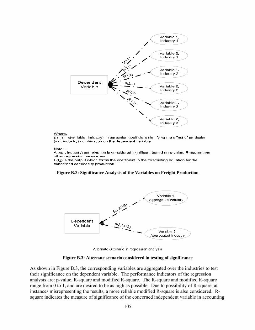
105

Figure B.2: Significance Analysis of the Variables on Freight Production

Figure B.3: Alternate scenario considered in testing of significance

As shown in Figure B.3, the corresponding variables are aggregated over the industries to test their significance on the dependent variable. The performance indicators of the regression analysis are: p-value, R-square and modified R-square. The R-square and modified R-square range from 0 to 1, and are desired to be as high as possible. Due to possibility of R-square, at instances misrepresenting the results, a more reliable modified R-square is also considered. R-square indicates the measure of significance of the concerned independent variable in accounting

106

for the variation in the dependent variable. Hence, the objective is to maximize R-square and control the p-value by employing different combination of variables and industry as discussed previously. This analysis is performed on all the concerned 42 commodity types.

B.1.1.4 Results of Freight Production The results of the freight production performed on all the commodity types considered are presented in Tables B.3 and B.4. The results presented include the following.

• Regression coefficients for the selected independent variable/industry for each of the commodity analyzed

• The result table also includes the R-square obtained, which is a measure of the effectiveness of the forecasting equations developed.

The results obtained in the freight production forms an input in the second step of the UTDM planning methodology.

B.1.2 Freight Attraction Another phase of freight generation is freight attraction. The objective of freight attraction is to evaluate the tonnage of freight that is consumed at each destination. A freight destination is a result of the attraction of that particular commodity type at the destination location. The attraction of freight to a particular location depends on factors like population and personal income. The population data is extracted from the Census database while the personal income data is extracted from the Bureau of Economic Analysis. The dependent variable is the destination tonnages, which are obtained from the CFS database. Once all the information has been compiled for all commodities, the regression equation is generated in Excel using the destination tonnage as dependent variable, and population and personal income as explanatory variables. The regression line expresses the best prediction of the dependent variable, given the explanatory variables. The regression coefficients represent the independent contributions of each independent variable to the prediction of the dependent variable. If the regression model results are not satisfactory (R-square is pretty low), then other explanatory variables are investigated. The variables that were investigated include production worker’s hours, production worker’s wages, cost of material, total value added, total capital expenditures and total value of shipments. The data for these variables are extracted from the CFS database. The regression analysis can be performed using Minitab or Excel. If co-linearity exists among the explanatory variables, some of the variables are removed from further investigations. All the other attraction regression analyses are carried out with the same methodology. The summary of attraction regression equations for all the other commodities along with their R-square are shown in the Table B.5.

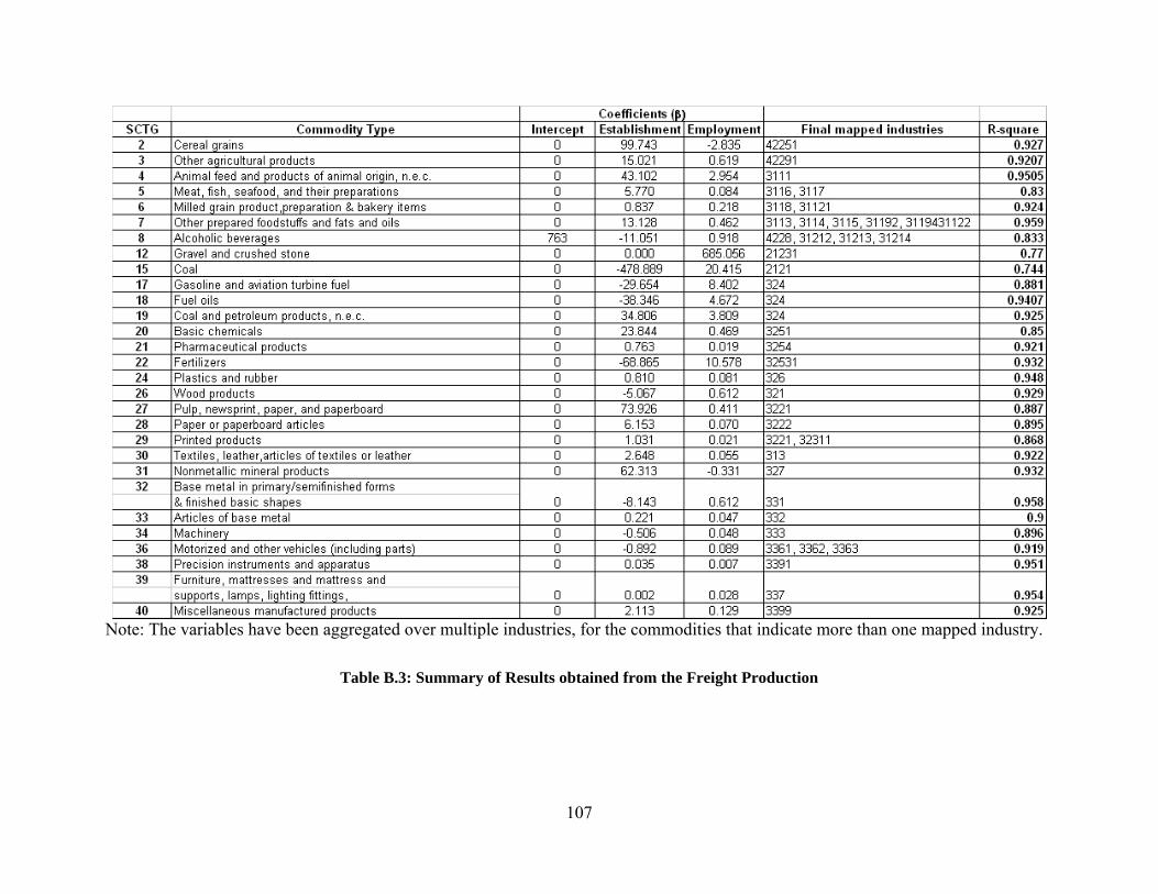
107

Note: The variables have been aggregated over multiple industries, for the commodities that indicate more than one mapped industry.

Table B.3: Summary of Results obtained from the Freight Production

108

Table B.4: Summary of Freight Production Output for Commodities that use Multiple Industries as Exclusive Independent Variables

109

SCTG Code – Commodity

R-Square Value

Explanatory Variable Explanatory Variable Coefficients

02 Cereal grains 0.76 Cost of Materials Total Value of Shipments Total Capital Expenditures

0.0208964 -0.0065589 -0.0766832

03 Other Agricultural Products 0.75

Cost of Materials Total Value of Shipments Production Workers Wages

0.0172065 -0.0048180 -0.0094272

04 Animal Feed and products of animal origins 0.88 Total Value of Shipments 0.0075627

05 Meat, fish, seafood and their preparation 0.88 Population

Personal Income 0.0002787 0.0018066

06 Milled grain products and preparations 0.94 Population

Personal Income 0.0003564 0.0032093

07 Other prepared foodstuffs and fats and oils

0.95 Population Personal Income

0.0013142 0.0154488

08 Alcoholic beverages 0.97 Population Personal Income

0.0003205 -0.0028732

09 Tobacco products 0.80 Population Personal Income

0.0000055 0.0006000

10 Monumental or building stone 0.84 Population

Personal Income 0.0000401 -0.0007548

11 Natural sands 0.93

Population Personal Income Operating Expenses Production Worker Wages

0.0019041 0.0719388 -0.0840313 -0.0321540

12 Gravel and crushed stones 0.85 Population

Personal Income 0.0049339 0.3970376

13 Nonmetallic minerals, n.e.c. 0.91 Cost of Materials

Total Capital Expenditure 0.0099432 -0.0289388

14 Metallic ores and concentrates 0.75

Production Worker Wages Value Added Total Value of Shipments

-0.1613036 -0.0402273 0.0513014

15 Coal 0.88 Number of Employees Sales, Shipments, Receipts

25.6496164 -0.0097379

17 Gasoline and aviation turbine fuel 0.76 Population

Personal Income 0.0038888 -0.1064077

18 Fuel Oils 0.73 Population Personal Income

0.0010948 0.0625725

19 Coal and petroleum products, n.e.c. 0.82 Population

Personal Income 0.0014944 -0.0062459

20 Basic chemicals 0.92 Total Capital Expenditures 0.0296018 21 Pharmaceutical products 0.89 Population

Personal Income 0.0000332 -0.0003563

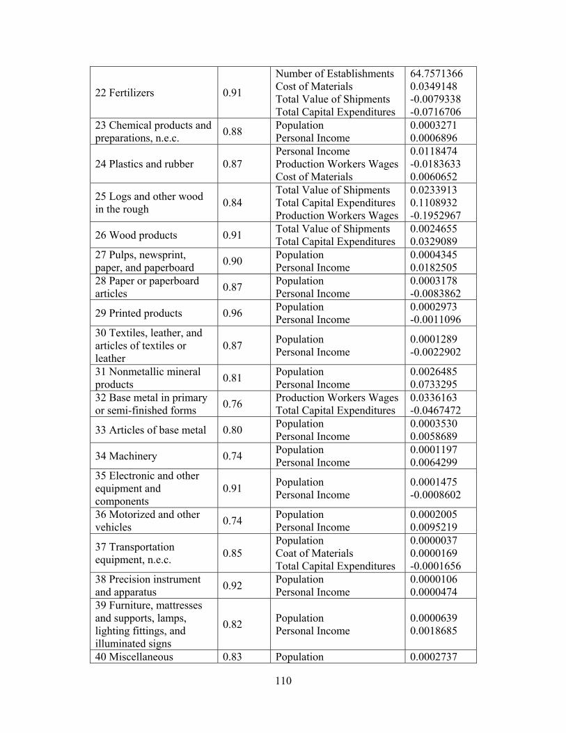
110

22 Fertilizers 0.91

Number of Establishments Cost of Materials Total Value of Shipments Total Capital Expenditures

64.7571366 0.0349148 -0.0079338 -0.0716706

23 Chemical products and preparations, n.e.c. 0.88 Population

Personal Income 0.0003271 0.0006896

24 Plastics and rubber 0.87 Personal Income Production Workers Wages Cost of Materials

0.0118474 -0.0183633 0.0060652

25 Logs and other wood in the rough 0.84

Total Value of Shipments Total Capital Expenditures Production Workers Wages

0.0233913 0.1108932 -0.1952967

26 Wood products 0.91 Total Value of Shipments Total Capital Expenditures

0.0024655 0.0329089

27 Pulps, newsprint, paper, and paperboard 0.90 Population

Personal Income 0.0004345 0.0182505

28 Paper or paperboard articles 0.87 Population

Personal Income 0.0003178 -0.0083862

29 Printed products 0.96 Population Personal Income

0.0002973 -0.0011096

30 Textiles, leather, and articles of textiles or leather

0.87 Population Personal Income

0.0001289 -0.0022902

31 Nonmetallic mineral products 0.81 Population

Personal Income 0.0026485 0.0733295

32 Base metal in primary or semi-finished forms 0.76 Production Workers Wages

Total Capital Expenditures 0.0336163 -0.0467472

33 Articles of base metal 0.80 Population Personal Income

0.0003530 0.0058689

34 Machinery 0.74 Population Personal Income

0.0001197 0.0064299

35 Electronic and other equipment and components

0.91 Population Personal Income

0.0001475 -0.0008602

36 Motorized and other vehicles 0.74 Population

Personal Income 0.0002005 0.0095219

37 Transportation equipment, n.e.c. 0.85

Population Coat of Materials Total Capital Expenditures

0.0000037 0.0000169 -0.0001656

38 Precision instrument and apparatus 0.92 Population

Personal Income 0.0000106 0.0000474

39 Furniture, mattresses and supports, lamps, lighting fittings, and illuminated signs

0.82 Population Personal Income

0.0000639 0.0018685

40 Miscellaneous 0.83 Population 0.0002737

111

manufactured products Personal Income 0.0105644

41 Waste and scrap 0.79 Population Personal Income

0.0005928 0.0135332

43 Mixed freight 0.92 Population Personal Income

0.0003804 0.0001165

Table B.5: Summary of Freight Attraction Output for all Commodities

B.2 Freight Distribution using a Doubly Constrained Gravity Model Regional freight distribution is to distribute freight generation (production and attraction) of a state/MSA to all other states/MSAs. The regional freight flow distribution was modeled using the doubly-constrained gravity model in TransCAD®. A doubly constrained gravity model ensures that the flow conservation of productions and attractions for each state/MSA. The distribution outcome is an O-D flow matrix for all states/MSAs. The following sections document the databases required for the doubly constrained gravity model (see Section 2.1.2.2 for gravity model details), and some sample results of freight distribution.

B.2.1 Databases Required for the Gravity Model Necessary input data needed to run the gravity model include:

• A state/MSA-to-state/MSA friction factor matrix or an impedance table. In our distribution, a distance-based friction factor matrix was used.

• A USA state/MSA zone layer with estimated productions and attractions from freight generation

• A layer of state/MSA population-weighted centroids The friction factor matrix is based on a state/MSA-to-state/MSA centroid distance matrix, which is commonly calculated in a mathematical function, such as gamma, exponential, or inverse power. The distance matrix itself can also be used as the input friction factor matrix. Since the regression estimated production and attractions include within state productions and attractions, each state’s estimated production and attraction were multiplied by a “instate factor”. The instate factor ensures that a state distributes its relevant production to all other states and attracts from other states the relevant freight that is distributed to the state. Using the instate factor, the total instate production and attraction were computed as an average of the instate production and attraction. Such distribution relevant productions and attractions must be stored in table fields that are either contained in a map zone layer or in a table that is joined to a zone layer. The totals of the productions and attractions must be equal; otherwise, a balance procedure is needed. Given that a state’s estimated attribution is more reliable, in the balance procedure, attraction was held constant to balance the production. An inverse function of distance was used to calculate the friction factor matrix.

112

B.2.2 Sample Results for Freight Distribution Figure B.4 and B.5 provide sample results for the commodity type “Furniture”. While Figure B.4 presents the state-to-state O-D furniture flows larger than 10,000 tons, Figure B.5 presents the O-D furniture From and To flows larger than 1,000 tons.

Figure B.4 State to State O-D Furniture Flows Larger than 10,000 tons

Figure B.5: O-D furniture From and To flows larger than 1,000 tons

B.3 Mode-Split Mode split is the process of allocating the total flows between states obtained by freight distribution among the various transportation modes like road, rail, water and air. In passenger transportation, mode choice analysis is a complex process that depends on the passengers’ perception of the advantages and disadvantages of a choice of a particular mode. In case of freight distribution, the mode-split process should also consider the relative advantages of different modes based on service levels, costs, and nature of the commodity [30].

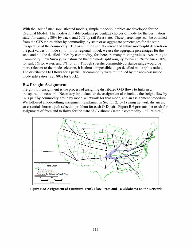
113

With the lack of such sophisticated models, simple mode-split tables are developed for the Regional Model. The mode-split table contains percentage choices of mode for the destination state, for example 80% by truck, and 20% by rail for a state. These percentages can be obtained from the CFS tables either by commodity, by state or as aggregate percentages for the state irrespective of the commodity. The assumption is that current and future mode-split depends on the past values of mode-split. In our regional model, we use the aggregate percentages for the state and not the detailed tables by commodity, for there are many missing values. According to Commodity Flow Survey, we estimated that the mode split roughly follows 80% for truck, 10% for rail, 5% for water, and 5% for air. Though specific commodity, distance range would be more relevant to the mode selection, it is almost impossible to get detailed mode splits ratios. The distributed O-D flows for a particular commodity were multiplied by the above-assumed mode split ratios (i.e., 80% for truck).

B.4 Freight Assignment Freight flow assignment is the process of assigning distributed O-D flows to links in a transportation network. Necessary input data for the assignment also include the freight flow by O-D pair by commodity group by mode, a network for that mode, and an assignment procedure. We followed all-or-nothing assignment (explained in Section 2.1.4.1) using network distances, an essential shortest-path selection problem for each O-D pair. Figure B.6 presents the result for assignment of from and to flows for the state of Oklahoma (sample commodity – “Furniture”).

Figure B.6: Assignment of Furniture Truck Flow From and To Oklahoma on the Network

114

APPENDIX C: COMBINED REGIONAL–STATE MODEL The following sections provide information about some of the inputs needed for the combined regional-state model, and the results for the year 2002.

C.1 Inputs to the Combined Regional-State Model This section presents the various FAF2 regions and the counties in the three MSAs in Oklahoma that form the centroids for the combined regional-state model and the payload factors that were used for converting the freight flows from tonnage to the number of trucks.

C.1.1 Centroids for the Combined Regional-State Model The centroids used in the combined regional-state model come from the FAF2 database [13]. The database consists of 114 regions (Table C.1). As discussed in Section 4.1, the research team added more centroids, representing the counties, in Oklahoma. This requires splitting the Oklahoma City region (OK Oklah) into 8 counties presented in Table C.2, the Tulsa region (OK Tulsa) into 8 counties presented in the Table C.3, and the remainder of Oklahoma (OK rem) into 61 counties (Table C.4). The list of Freight Analysis Framework-2 regions are as follows.

ID BTS/Census Commodity Flow Survey Region Name

FAF Database Abbreviation

FAF Region

1 Birmingham-Hoover-Cullman, AL CSA AL Birmi AL 2 Remainder of Alabama AL rem AL 3 Alaska AK AK 4 Phoenix-Mesa-Scottsdale, AZ MSA AZ Phoen AZ 5 Tucson, AZ MSA AZ Tucso AZ 6 Remainder of Arizona AZ rem AZ 7 Arkansas AR AR 8 Los Angeles-Long Beach-Riverside, CA CSA CA Los A CA 9 San Diego-Carlsbad-San Marcos, CA MSA CA San D CA

10 Sacramento--Arden-Arcade--Truckee, CA-NV CSA (CA Part)

CA Sacra CA

11 San Jose-San Francisco-Oakland, CA CSA CA San J CA 12 Remainder of California CA rem CA 13 Denver-Aurora-Boulder, CO CSA CO Denve CO 14 Remainder of Colorado CO rem CO 15 New York-Newark-Bridgeport, NY-NJ-CT-PA

CSA (CT Part) CT New Y CT

16 Remainder of Connecticut CT rem CT 17 Delaware DE DE 18 Washington-Arlington-Alexandria, DC-VA-MD-

WV MSA (DC Part) DC Washi DC

19 Jacksonville, FL MSA FL Jacks FL 20 Miami-Fort Lauderdale-Miami Beach, FL MSA FL Miami FL 21 Orlando-The Villages, FL CSA FL Orlan FL 22 Tampa-St Petersburg-Clearwater, FL MSA FL Tampa FL 23 Remainder of Florida FL rem FL

115

24 Atlanta-Sandy Springs-Gainesville, GA-AL CSA (GA Part)

GA Atlan GA

25 Remainder of Georgia GA rem GA 26 Honolulu, HI MSA HI Honol HI 27 Remainder of Hawaii HI rem HI 28 Idaho ID ID 29 Chicago-Naperville-Michigan City, IL-IN-WI CSA

(IL Part) IL Chica IL

30 St Louis, MO-IL MSA (IL Part)

IL St Lo IL

31 Remainder of Illinois IL rem IL 32 Chicago-Naperville-Michigan City, IL-IN-WI CSA

(IN Part) IN Chica IN

33 Indianapolis-Anderson-Columbus, IN CSA IN India IN 34 Remainder of Indiana IN rem IN 35 Iowa IA IA 36 Kansas City, MO-KS MSA (KS Part) KS Kansa KS 37 Remainder of Kansas KS rem KS 38 Louisville-Elizabethtown-Scottsburg, KY-IN CSA

(KY Part) KY Louis KY

39 Remainder of Kentucky KY rem KY 40 New Orleans-Metairie-Bogalusa, LA CSA LA New O LA 41 Remainder of Louisiana LA rem LA 42 Maine ME ME 43 Baltimore-Towson, MD MeSA MD Balti MD 44 Washington-Arlington-Alexandria, DC-VA-MD-

WV MeSA (MD Part) MD Washi MD

45 Remainder of Maryland MD rem MD 46 Boston-Worcester-Manchester, MA-NH CSA (MA Part) MA Bosto MA 47 Remainder of Massachusetts MA rem MA 48 Detroit-Warren-Flint, MI CSA MI Detro MI 49 Grand Rapids-Wyoming-Holland, MI CSA MI Grand MI 50 Remainder of Michigan MI rem MI 51 Minneapolis-St Paul-St Cloud, MN-WI CSA (MN

Part) MN Minne

MN

52 Remainder of Minnesota MN rem MN 53 Mississippi MS MS 54 Kansas City, MO-KS MeSA (MO Part) MO Kansa MO 55 St Louis-St Charles-Farmington, MO-IL CSA (MO

Part) MO St Lo MO

56 Remainder of Missouri MO rem MO 57 Montana MT MT 58 Nebraska NE NE 59 Las Vegas-Paradise-Pahrump, NV CSA NV Las V NV 60 Remainder of Nevada NV rem NV 61 New Hampshire NH NH 62 New York-Newark-Bridgeport, NY-NJ-CT-PA

CSA (NJ Part) NJ New Y NJ

63 Philadelphia-Camden-Vineland, PA-NJ-DE-MD NJ Phila NJ

116

CSA (NJ Part) 64 Remainder of New Jersey NJ rem NJ 65 New Mexico NM NM 66 Albany-Schenectady-Amsterdam, NY CSA NY Alban NY 67 Buffalo-Cheektowaga-Tonawanda, NY MeSA NY Buffa NY 68 New York-Newark-Bridgeport, NY-NJ-CT-PA

CSA (NY Part) NY New Y NY

69 Rochester-Batavia-Seneca Falls, NY CSA NY Roche NY 70 Remainder of New York NY rem NY 71 Charlotte-Gastonia-Salisbury, NC-SC CSA (NC

Part) NC Charl NC

72 Greensboro—Winston-Salem—High Point, NC CSA NC Green NC 73 Raleigh-Durham-Cary, NC CSA NC Ralei NC 74 Remainder of North Carolina NC rem NC 75 North Dakota ND ND 76 Cincinnati-Middletown-Wilmington, OH-KY-IN

CSA (OH Part) OH Cinci OH

77 Cleveland-Akron-Elyria, OH CSA OH Cleve OH 78 Columbus-Marion-Chillicothe, OH CSA OH Colum OH 79 Dayton-Springfield-Greenville, OH CSA OH Dayto OH 80 Remainder of Ohio OH rem OH 81 Oklahoma City-Shawnee, OK CSA OK Oklah OK 82 Tulsa-Bartlesville, OK CSA OK Tulsa OK 83 Remainder of Oklahoma OK rem OK 84 Portland-Vancouver-Beaverton, OR-WA MeSA

(OR Part) OR Portl OR

85 Remainder of Oregon OR rem OR 86 Philadelphia-Camden-Vineland, PA-NJ-DE-MD

CSA (PA Part) PA Phila PA

87 Pittsburgh-New Castle, PA CSA PA Pitts PA 88 Remainder of Pennsylvania PA rem PA 89 Rhode Island RI RI 90 Greenville-Anderson-Seneca, SC CSA SC Green SC 91 Spartanburg-Gaffney-Union, SC CSA SC Spart SC 92 Remainder of South Carolina SC rem SC 93 South Dakota SD SD 94 Memphis, TN-MS-AR MeSA (TN Part) TN Memph TN 95 Nashville-Davidson--Murfreesboro--Columbia, TN

CSA TN Nashv TN

96 Remainder of Tennessee TN rem TN 97 Austin-Round Rock, TX MeSA TX Austi TX 98 Dallas-Fort Worth, TX CSA TX Dalla TX 99 Houston-Baytown-Huntsville, TX CSA TX Houst TX

100 San Antonio, TX MeSA TX San A TX 101 Remainder of Texas TX rem TX 102 Salt Lake City-Ogden-Clearfield, UT CSA UT Salt UT 103 Remainder of Utah UT rem UT 104 Vermont VT VT 105 Richmond, VA MeSA VA Richm VA

117

106 Virginia Beach-Norfolk-Newport News, VA-NC MeSA (VA Part)

VA Virgi VA

107 Washington-Baltimore-Northern Virginia, DC- MD-VA-WV CSA (VA Part)

VA Washi VA

108 Remainder of Virginia VA rem VA 109 Seattle-Tacoma-Olympia, WA CSA WA Seatt WA 110 Remainder of Washington WA rem WA 111 West Virginia WV WV 112 Milwaukee-Racine-Waukesha, WI CSA WI Milwa WI 113 Remainder of Wisconsin WI rem WI 114 Wyoming WY WY

Table C.1: Freight Analysis Framework–2 Regions

The following counties are included in the Oklahoma City region.

ID County 1 Canadian 2 Cleveland 3 Grady 4 Lincoln 5 Logan 6 McClain 7 Oklahoma 8 Pottawatomie

Table C.2: Counties included in Oklahoma City Region (OK Oklah)

The following counties are included in the Tulsa region.

ID County 1 Creek 2 Okmulgee 3 Osage 4 Pawnee 5 Rogers 6 Tulsa 7 Wagoner 8 Washington

Table C.3: Counties included in Tulsa Region (OK Tulsa)

118

The following counties are included in the remainder of OK.

ID County 1 Adair 2 Alfalfa 3 Atoka 4 Beaver 5 Beckham 6 Blaine 7 Bryan 8 Caddo 9 Carter

10 Cherokee 11 Choctaw 12 Cimarron 13 Coal 14 Comanche 15 Cotton 16 Craig 17 Custer 18 Delaware 19 Dewey 20 Ellis 21 Garfield 22 Garvin 23 Grant 24 Greer 25 Harmon 26 Harper 27 Haskell 28 Hughes 29 Jackson 30 Jefferson 31 Johnston 32 Kay 33 Kingfisher 34 Kiowa 35 Latimer 36 Le Flore 37 Love 38 McCurtain 39 McIntosh 40 Major 41 Marshall 42 Mayes 43 Murray 44 Muskogee 45 Noble 46 Nowata

119

47 Okfuskee 48 Ottawa 49 Payne 50 Pittsburg 51 Pontotoc 52 Pushmataha 53 Roger Mills 54 Seminole 55 Sequoyah 56 Stephens 57 Texas 58 Tillman 59 Washita 60 Woods 61 Woodward

Table C.4: Counties included in Remainder of Oklahoma (OK rem)

C.1.2 Payload Factors for Tonnage to Number of Trucks Conversion The payload factors, as discussed in Section 4.3.3, are required to convert the freight flows from tonnage to number of trucks. This conversion is especially needed in the case of capacitated freight assignment as the capacities on the various links are furnished in terms of number of trucks, while the freight flow data is in terms of tonnage. The payload factor by distance developed by Cambridge Systematics for each commodity is as follows [12].

SCTG Code

SCTG Commodity Description Local (< 50 miles)

Short (50 – 100

miles)

Short-Medium

(100 – 200

miles)

Long –Medium

(200 – 500

miles)

Long (>

500 miles)

1 Live animals and live fish 12.04 18.37 19.1 18.71 17.67 2 Cereal grains 12.04 18.37 19.1 18.71 17.67 3 Other agricultural products 13.36 11.64 13.27 13.27 13.27 4 Animal feed and products of animal

origin, n.e.c. 12.04 18.37 19.1 18.71 17.67

5 Meat, fish, seafood, and their preparations

8.2 8.13 14.42 15.89 16.11

6 Milled grain products and preparations, and bakery products

8.2 8.13 14.42 15.89 16.11

7 Other prepared foodstuffs and fats and oils

8.2 8.13 14.42 15.89 16.11

8 Alcoholic beverages 8.2 8.13 14.42 15.89 16.11 9 Tobacco products 11.5 16.25 16.03 11.47 15.96

10 Monumental or building stone 16.98. 18.81 25.77 25.77 25.77 11 Natural sands 16.98. 18.81 25.77 25.77 25.77 12 Gravel and crushed stone 16.98. 18.81 25.77 25.77 25.77 13 Nonmetallic minerals, n.e.c. 16.98. 18.81 25.77 25.77 25.77 14 Metallic ores and concentrates 16.98. 18.81 25.77 25.77 25.77 15 Coal 16.98. 18.81 25.77 25.77 25.77

120

16 - 14.43 19.58 17.84 17.84 17.84 17 Gasoline and aviation turbine fuel 14.43 19.58 17.84 17.84 17.84 18 Fuel oils 14.43 19.58 17.84 17.84 17.84 19 Coal and petroleum products, n.e.c. 14.43 19.58 17.84 17.84 17.84 20 Basic chemicals 5.18 15.39 19.55 19.25 19.25 21 Pharmaceutical products 5.18 15.39 19.55 19.25 19.25 22 Fertilizers 5.18 15.39 19.55 19.25 19.25 23 Chemical products and

preparations, n.e.c. 5.18 15.39 19.55 19.25 19.25

24 Plastics and rubber 7.05 4.42 11.47 9.84 11.3 25 Logs and other wood in the rough 10.33 12.35 17.5 17.61 17.83 26 Wood products 10.33 12.35 17.5 17.61 17.83 27 Pulp, newsprint, paper, and

paperboard 4.07 7.67 15.66 15.17 14.59

28 Paper or paperboard articles 4.07 7.67 15.66 15.17 14.59 29 Printed products 4.07 7.67 15.66 15.17 14.59 30 Textiles, leather, and articles of

textiles or leather 1.34 3.57 18.18 18.16 17.48

31 Nonmetallic mineral products 10.69 14.47 18.53 18.63 18.81 32 Base metal in primary or semi-

finished forms and in finished basic shapes

11.82 14.73 19.96 20.14 20.13

33 Articles of base metal 4.00 11.33 14.49 14.49 14.49 34 Machinery 6.97 12.55 17.42 17.21 17.21 35 Electronic and other electrical

equipment and components, and office equipment

4.05 7.42 14.81 14.62 14.62

36 Motorized and other vehicles (including parts)

2.48 14.12 17.21 16.92 14.18

37 Transportation equipment, n.e.c. 2.48 14.12 17.21 16.92 14.18 38 Precision instruments and apparatus 6.97 12.55 17.42 17.21 17.21 39 Furniture, mattresses and supports,

lamps, lighting fittings, and illuminated signs

2.92 3.25 11.02 11.26 11.38

40 Miscellaneous manufactured products

5.48 5.4 11.63 13.04 14.23

41 Waste and scrap 5.48 5.4 11.63 13.04 14.23 43 Mixed freight 5.48 5.4 11.63 13.04 14.23

Table C.5: Payload Factor by Distance for each Commodity

C.2 Flow Assignment Results for Base Year (2002) The results for the base year 2002 are presented in the following sections.

C.2.1 Total flow on each network The results of all assignment algorithms for the highway network in the year 2002 are illustrated in Figures C.1 – C.4.

121

Figure C.1: Total Flow on Highway Network in 2002 by All-or-Nothing Assignment

Figure C.2: Total Flow on Highway Network in 2002 by System Optimal Assignment

122

Figure C.3: Total Flow on Highway Network in 2002 by User Equilibrium Assignment

Figure C.4: Total Flow on Highway Network in 2002 by Stochastic User Equilibrium Assignment

For railway and waterway networks, the only assignment algorithm used is All-or-Nothing because it is assumed that both networks are un-capacitated. The results of the total flow assigned on these networks are shown in Figures C.5 – C.8.

123

Figure C.5: Total Flow on Railway Network in 2002 in U.S.

Figure C.6: Total Flow on Railway Network in 2002 in Oklahoma

124

Figure C.7: Total Flow on Waterway Network in 2002 in U.S.

Figure C.8: Total Flow on Waterway Network in 2002 in Oklahoma

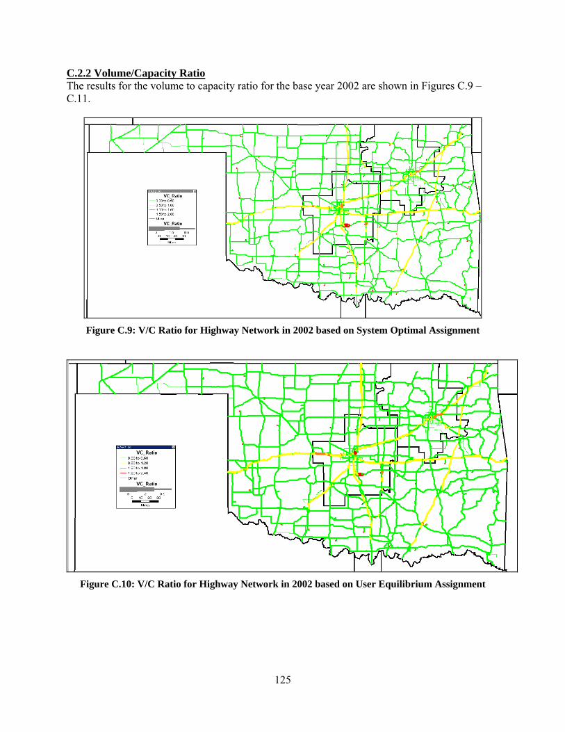
125

C.2.2 Volume/Capacity Ratio The results for the volume to capacity ratio for the base year 2002 are shown in Figures C.9 – C.11.

Figure C.9: V/C Ratio for Highway Network in 2002 based on System Optimal Assignment

Figure C.10: V/C Ratio for Highway Network in 2002 based on User Equilibrium Assignment

126

Figure C.11: V/C Ratio for Highway Network in 2002 based on Stochastic User Equilibrium

Assignment

C.2.3 Flow by flow type For All-or-Nothing assignment, total flow on the highway network can be further disaggregated into flow types comprising of From, To, Through and Within. Figures C.12 – C.15 illustrate flow by each flow type on the highway network.

Figure C.12: Flow Map for Total From-Flow on Highway Network in 2002

127

Figure C.13: Flow Map for Total To-Flow on Highway Network in 2002

Figure C.14: Flow Map for Total Within-Flow on Highway Network in 2002

128

Figure C.15: Flow Map for Total Through-Flow on Highway Network in 2002

C.2.4 Top Commodities for Oklahoma Another interesting set of results that can be obtained from the freight flow assignment is the list of top commodities in Oklahoma. Tables C.6 – C.8 illustrate top commodities that have a destination in Oklahoma by each transport mode, while Tables C.9 – C.11 illustrate the list of top commodities that originate from Oklahoma for each mode.

Destination State Commodity Mode Kton/year

OK Cereal grains Truck 75145.89 OK Gravel Truck 26117.17 OK Other ag prods. Truck 19643.03 OK Nonmetal min. prods. Truck 16067.52 OK Unknown Truck 15949.14 OK Waste/scrap Truck 15191.60 OK Articles-base metal Truck 10018.79 OK Coal-n.e.c. Truck 8451.92 OK Other foodstuffs Truck 8189.01 OK Live animals/fish Truck 7444.66

Table C.6: Top Commodities Coming into Oklahoma by Truck in 2002

129

Destination State Commodity Mode Kton/year

OK Coal Rail 14054.60 OK Natural sands Rail 2543.58 OK Waste/scrap Rail 1750.86 OK Wood prods. Rail 1483.37 OK Coal-n.e.c. Rail 1111.19 OK Gravel Rail 1052.67 OK Nonmetal min. prods. Rail 664.74 OK Cereal grains Rail 600.28 OK Other foodstuffs Rail 494.85 OK Animal feed Rail 298.06

Table C.7: Top Commodities Coming into Oklahoma by Rail in 2002

Destination State Commodity Mode Kton/year

OK Fertilizers Water 951.27 OK Base metals Water 165.75 OK Articles-base metal Water 14.71

Table C.8: Top Commodities Coming into Oklahoma by Waterway in 2002

Origin Commodity Mode Kton/year OK Cereal grains Truck 76544.01 OK Gravel Truck 26435.40 OK Other ag prods. Truck 21027.17 OK Unknown Truck 17944.44 OK Nonmetal min. prods. Truck 16818.73 OK Waste/scrap Truck 15716.06 OK Articles-base metal Truck 10833.68 OK Coal-n.e.c. Truck 10592.82 OK Live animals/fish Truck 7912.09 OK Other foodstuffs Truck 7078.82

Table C.9: Top Commodities Going out of Oklahoma by Truck in 2002

130

Origin Commodity Mode Kton/year OK Gravel Rail 7962.26 OK Fertilizers Rail 2707.75 OK Natural sands Rail 2700.96 OK Coal-n.e.c. Rail 2376.37 OK Waste/scrap Rail 1578.00 OK Motorized vehicles Rail 860.31 OK Newsprint/paper Rail 849.41 OK Plastics/rubber Rail 289.86 OK Base metals Rail 197.22 OK Nonmetal min. prods. Rail 169.00

Table C.10: Top Commodities Going out of Oklahoma by Rail in 2002

Origin Commodity Mode Kton/year OK Fertilizers Water 301.87 OK Cereal grains Water 229.31 OK Other ag prods. Water 3.94

Table C.11: Top Commodities Going out of Oklahoma by Waterway in 2002

C.2.5 Top Trading Partners for Oklahoma The following tables present the top trading partners for Oklahoma, i.e. the top few regions which attract commodities produced in Oklahoma (Tables C.12 – C.14) or the top regions from which commodities are shipped to Oklahoma (Tables C.15 – C.17).

Origin Destination Mode Kton/YearOK TX Truck 17825.75OK AR Truck 7854.19OK KS Truck 7692.83OK MO Truck 3785.83OK CA Truck 739.01OK GA Truck 601.81OK NJ Truck 594.03OK OH Truck 543.65OK IL Truck 541.16OK AL Truck 536.51

Table C.12: Top Trading Partners Receiving Commodities from Oklahoma by Truck in 2002

131

Origin Destination Mode Kton/YearOK TX Rail 8858.58OK MO Rail 812.61OK NE Rail 711.36OK AR Rail 671.11OK IA Rail 666.32OK CA Rail 442.10OK KS Rail 429.88OK IN Rail 287.79OK CO Rail 277.45OK GA Rail 252.36

Table C.13: Top Trading Partners Receiving Commodities from Oklahoma by Rail in 2002

Origin Destination Mode Kton/YearOK TN Water 394.32OK LA Water 138.63OK MN Water 2.17

Table C.14: Top Trading Partners Receiving Commodities from Oklahoma by Waterway in 2002

Origin Destination Mode Kton/YearKS OK Truck 10112.20TX OK Truck 7660.59AR OK Truck 4697.82MO OK Truck 3427.29GA OK Truck 1393.34IA OK Truck 846.22OH OK Truck 840.31LA OK Truck 747.04CO OK Truck 732.18NC OK Truck 617.45

Table C.15: Top Trading Partners Sending Commodities to Oklahoma by Truck in 2002

132

Origin Destination Mode Kton/YearWY OK Rail 14263.66AR OK Rail 1576.07MO OK Rail 1180.23TX OK Rail 494.28IA OK Rail 459.53IN OK Rail 407.87KS OK Rail 381.43AL OK Rail 332.59NE OK Rail 253.44CO OK Rail 216.90

Table C.16: Top Trading Partners Sending Commodities to Oklahoma by Rail in 2002

Origin Destination Mode Kton/YearLA OK Water 910.78IN OK Water 165.75IL OK Water 40.49KY OK Water 14.71

Table C.17: Top Trading Partners Sending Commodities to Oklahoma by Waterway in 2002

133

APPENDIX D: CAPACITATED NETWORK FREIGHT ASSIGNMENT USING SIMPLIFIED PIECEWISE LINEAR TRAVEL-TIME FUNCTION

The research team has developed an optimization model that can assign freight to links in a network, essentially replacing the flow assignment step currently performed using TransCAD®. The motivation for the model came from the fact that initially the travel time increases gradually with the traffic flow until a particular point, after which it increases at a much higher rate as seen in the work of Ortuzar and Willumsen [33]. It was decided that the optimization model would take into account link capacities. As a result, the cost in the objective function would be in terms of the travel time. The following sections present the motivation behind the optimization model, the model details, some preliminary results and issues that need to be addressed in implementing the model.

D.1 Travel-Time Flow Curves For a congested network, the cost-flow or travel time flow curves, as shown in Figure D.1, are used to represent the relationship between link flows and link performances [33]. The dashed line in Figure D.1 shows the estimation of speed and travel time when flow volume approaches the capacity of the link.

Figure D.1 Travel Time-Flow Curve [33]

Some of the cost-flow relationships proposed by researchers are as follows. Smock [34] for Detroit Study

t = t0 exp (V/C) D.1 Overgaard [35] t = t0 αβ(V/C) D.2

134

Bureau of Public Roads [32] in the U.S. t = t0 [1 + α(V/C)β] D.3 where V Link volume in passenger car equivalent unit/hour (e.g. passenger car equivalent unit is

flow volume unit equivalent converting all types of vehicles on a link into passenger cars.)

C Link capacity in passenger car equivalent unit/hour t Congested travel time of the link t0 Free-flow travel time of the link α, β Parameters in the model As discussed in Section 4.2.1, the cost-flow relationship provided by the Bureau of Public Roads [32] was in used our study. It can be seen that the travel time expression, which would form part of our objective function is non-linear. The team tried to resolve this issue by using a simplified (approximate) travel time curve as follows.

Figure D.2: Simplified Travel-Time Flow Curve

The simplified travel-time curve expresses the travel time curve as a piece-wise linear functions, where the flow is distinguished as free flow and congested flow. It is assumed that free flow occurs until the free flow threshold on the link, denoted by x in Figure D.2, is reached. Beyond the threshold, the flow would be congested. Thus, the travel time can be expressed using the following equation. D.4

⎩⎨⎧

>∗+≤

= thresholdflow free flowrate flow congested timeflow free thresholdflow free flow timeflow free

timeTravel

135

D.2 Formulation of the Freight Flow Assignment Problem The objective of the optimization model is to assign freight flow to the highway network so as to minimize the sum of travel time over all links. In the model, we assume that when the flow volume exceeds the free flow threshold of the link, there is a higher penalty on freight flow. This would force the optimization model to choose an alternative route. The various constraints for this model are the flow balance constraints, free flow threshold constraints, binary variable constraints, and non-negativity constraints. The decision variables, the parameters, and the formulation are presented in the following section.

D.2.1 Model Nomenclature The model nomenclature consists of the model parameters and decision variables. The model parameters indicate the inputs that go into the optimization model and the model decision variables represent the variables that the optimization model has to determine.

D.2.1.1 Model Parameters The model parameters are as follows. L Set of all links (i j) Directed arc from node i to node j Cij Free flow threshold on (i j) Fij Free-flow travel time on (i j) Rij Rate at which the congested travel time increases on (i j) Dk Truck flow volume for OD pair k

D.2.1.2 Model Decision variables The model decision variables are as follows. xi,j,k Free-flow truck volume on (i j) corresponding to OD pair k yi,j,k Congested truck volume on (i j) corresponding to OD pair k zij Binary variable indicating flow on (i j) wij Binary variable indicating congested flow on (i j)

D.2.2 Model Objective and Constraints The model formulation consists of the objective function and the various constraints placed on the model due to free flow threshold restrictions on the links, flow balance, binary variables, and the non-negativity of flow.

D.2.2.1 Objective Function

⎭⎬⎫

⎩⎨⎧

⎥⎦

⎤⎢⎣

⎡+∑ ∑

∈Lji kijijkijij RyFz

)(min D.5

The objective of this problem is to minimize the sum of travel time over all links. When the flow on a link is less than the free flow threshold of the link, expression D.5 reduces to the product of

136

the binary variable zi,j and the free-flow travel time Fij. This is because there will be no congested traffic flow in this range. But, when the threshold is exceeded, a heavier penalty (cost) is added to the free-flow travel time as shown in expression D.5. As a result, the total travel time of links in this range of traffic flow would be expression D.5.

D.2.2.2 Flow Balance Constraints for each OD pair k

{ }{ } ⎪⎩

⎪⎨

⎧

=∀=∀

≠≠∀

−=+−+∑ ∑

∈ ∈ kDiikOii

kDiOii

DDyxyx

k

kLjij Lijj

jikjikijkijk

pairODfor|pairODfor|

pairODfor&|0)()(

)(| )(|

D.6

The flow balance constraint in expression D.6 states that the net flow out of a node is zero if the node is a transshipment node (neither an origin nor destination of O-D pair k). When a node is the origin of O-D pair k, then the net flow out of that node is equal to the demand corresponding to the O-D pair k. Similarly, when a node is the destination of OD pair k, the net flow out of the node is equal to the negative of the demand corresponding to OD pair j.

D.2.2.3 Free Flow Threshold Constraints

LjiCzxk

ijijijk ∈∀⋅≤∑ )( D.7

LjiCwx

kijijijk ∈∀⋅≥∑ )( D.8

LjiDwy

k kkijijk ∈∀≤∑ ∑ )( D.9

The free flow threshold constraint D.7 ensures that the free flow volume on a link does not exceed the free flow threshold on that link. The constraints D.8 and D.9 ensure that there is no congested flow assigned on a link when the free flow threshold on the link has not been reached.

D.2.2.4 Binary Variable Constraints

{ } kLjiwz ijij ∀∈∀∈ ;)(1,0, D.10 The above constraint D.10 states that the decision variables can only take binary values.

D.2.2.5 Non-Negativity Constraints

kLjiyx ijkijk ∀∈∀≥ ;)(0, D.11 The above non-negativity constraint D.11 states that the decision variables can never take a negative value.

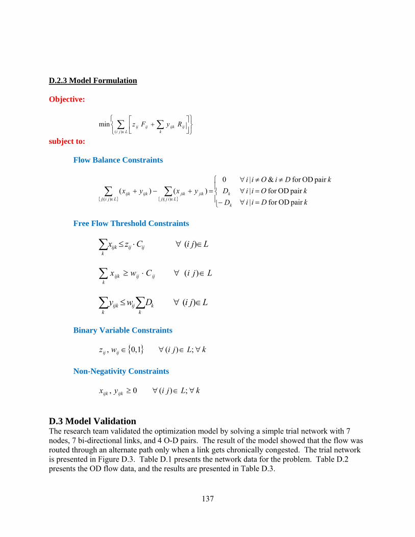
137

D.2.3 Model Formulation Objective:

⎭⎬⎫

⎩⎨⎧

⎥⎦

⎤⎢⎣

⎡+∑ ∑

∈Lji kijijkijij RyFz

)(min

subject to: Flow Balance Constraints

{ }{ } ⎪

⎩

⎪⎨

⎧

=∀=∀

≠≠∀

−=+−+∑ ∑

∈ ∈ kDiikOii

kDiOii

DDyxyx

k

kLjij Lijj

jikjikijkijk

pairODfor|pairODfor|

pairODfor&|0)()(

)(| )(|

Free Flow Threshold Constraints

LjiCzx

kijijijk ∈∀⋅≤∑ )(

LjiCwx

kijijijk ∈∀⋅≥∑ )(

LjiDwy

k kkijijk ∈∀≤∑ ∑ )(

Binary Variable Constraints

{ } kLjiwz ijij ∀∈∀∈ ;)(1,0,

Non-Negativity Constraints kLjiyx ijkijk ∀∈∀≥ ;)(0,

D.3 Model Validation The research team validated the optimization model by solving a simple trial network with 7 nodes, 7 bi-directional links, and 4 O-D pairs. The result of the model showed that the flow was routed through an alternate path only when a link gets chronically congested. The trial network is presented in Figure D.3. Table D.1 presents the network data for the problem. Table D.2 presents the OD flow data, and the results are presented in Table D.3.

138

Figure D.3: Trial Network with 7 Nodes, 7 Bi-Directional Links, and 4 O-D Pairs

Arc # i j C(i,j) Ft(i,j) 1 1 2 57.3 0.12 2 2 1 57.3 0.12 3 2 3 28.65 0.21 4 3 2 28.65 0.21 5 3 4 34.38 0.26 6 4 3 34.38 0.26 7 4 5 17.19 0.31 8 5 4 17.19 0.31 9 2 5 34.38 0.20 10 5 2 34.38 0.20 11 3 6 17.19 0.18 12 6 3 17.19 0.18 13 4 7 34.38 0.25 14 7 4 34.38 0.25 15 3 5 28.65 0.45 16 5 3 28.65 0.45

Table D.1: Network Data

139

OD # O D Flow (OD #) 1 1 6 300 2 1 7 500 3 6 7 275 4 3 5 350

Table D.2: OD Flow Data

Arc ID Origin Destination OD Pair FreeFlowVol CongFlowVol TotFlow

1 1 2 1 0.00 300.00 300.00 1 1 2 2 57.27 442.73 500.00 3 2 3 1 28.63 271.37 300.00 3 2 3 2 0.00 34.36 34.36 5 3 4 2 34.36 0.00 34.36 5 3 4 3 0.00 275.00 275.00 8 5 4 2 17.18 448.46 465.64 9 2 5 2 34.36 431.28 465.64 11 3 6 1 17.18 282.82 300.00 12 6 3 3 17.18 257.82 275.00 13 4 7 2 34.36 465.64 500.00 13 4 7 3 0.00 275.00 275.00 15 3 5 4 28.63 321.37 350.00

Table D.3: Flow Assignment Results for Links with Positive Flow

D.4 Model Issues After validating the model using a small problem instance, the research team tried to solve the full network (171,172 bi-directional links and 135,594 nodes) with 2,472 O-D pairs and the problem seems to be very large to solve. The research team could solve the problem for the whole network with 4 OD pairs using Xpress-MP. It took 12 hours to read the data and build the problem and a further 1.5 hours to solve the problem. Any larger problem consumed the entire memory of the system. This necessitates alternate approaches to solving the model. The research team is in the process of simplifying the network using two different approaches. The first approach is to select the highway network by proximity to Oklahoma. A detailed highway network can be selected in Oklahoma and the neighboring states, while we can choose only the major highways as we move farther away from Oklahoma. The second approach is to solve the k-shortest path problem for each OD pair. Then the new simplified network could be the union of all the links that were part of the k-shortest path problem for all the OD pairs. Another approach is to exploit the structure of the problem. As per our formulation, we see that there are a set of variables which are part of the flow balance constraints for one OD pair only, which gives rise to a block diagonal structure. The research team aims to come up with an efficient algorithm to solve the problem.

140

APPENDIX E: USER’S MANUAL FOR FREIGHT LOGISTICS INFRASTRUCTURE PLANNING SOFTWARE (FLIPS)

E.1 Installation Instructions

Software Requirements: a. .NET Framework 2.0 (included in the CD) b. MapWindow GIS Application (included in the CD) c. MS EXCEL (not included in the CD)

The following steps are to be followed for setting up the application.

Install .NET Framework 2.0 (dotnetfx) which is provided in the CD

Install MapWindow GIS application (MapWindow46SR) provided in the CD using the following path C:\Program Files

When MapWindow GIS application is installed a new folder named MapWindow would

be created inside C:\Program Files

Copy the folder GISProject and paste inside the MapWindow folder, i.e. inside C:\Program Files\MapWindow

In order to run the application double click on the MapApplication – Run (exe file) available inside C:\Program Files\MapWindow\GISProject

141

E.2 Getting Started To start the application, double click on the shortcut icon named MapApplication – Run which is present in C:\Program Files\MapWindow\GISProject. The main window Oklahoma Freight Flow Analysis appears on the screen. This main window consists of three menu items. 1. File 2. Applications 3. Help

E.3 File Menu The “File” menu is used for closing the windows and exiting the application. The “Applications” menu has options to view results and Summaries of Freight Flow, to perform Queries and Advanced Queries using MapWindow GIS application. The Help menu has information about the FLIPS software and a user manual for the application. The File Menu has three items.

1. Close Current Window is used to close the window which is currently open.

2. Close All Windows is used to close all windows except the main window.

3. Exit is used to exit the application.

E.4 Applications Menu Applications Menu has Freight Flow Summaries, Basic Queries and GIS Application Advanced Queries submenus.

142

E.4.1 Freight Flow Summaries Freight Flow Summaries menu helps the user to see the results of Total Flow and Volume to Capacity Ratio for various years and for various modes. We can also view the reports (not implemented in this version) related to Production and Attraction Flows, Population and Employment, Critical Path Analysis, Top Commodities and Top Trading Partners.

E.4.1.1 Results: The Results menu leads to the screen shown below. In this screen, we have to select the Mode, the Year and Type of Result (Total Flow or Volume to Capacity Ratio) .

After selecting the Mode, Year and the Result click on Show Map button. The following screen will be displayed.

143

E.4.2 Basic Queries This menu is used to query and view results in the form of maps and tables. Queries are available for High Flow Volume, Top Links and Volume Capacity Ratio for various modes and various years. When the Basic Queries menu is selected the following Query window will be opened.

In order to run a query, select the mode, year and type of query and click on the OK button. The following query window will open. To run Top Links Query, select mode, year and query type as

144

Top Links and click on OK button. The Top Links query window, for the selected year and selected mode will open.

Enter the input value, select Show Map for viewing result in Map and Show Data for viewing result in Table formats. To run the same query with different input values, click the Clear button and enter the new values. To run High Flow Volume query select mode, year and query type as High Flow Volume and click on the OK button. The High Flow Volume query window, for the selected year and selected mode will open.

Enter the input value, select Show Map for viewing result as Map and Show Data for viewing result in a table format.

145

To run the same query with different input values, click the Clear button and enter the new values. The Zoom menu in the query window is used to perform Zoom In, Zoom Out, Pan and View the map in Full Extent activities. The Volume to Capacity Ratio is available only for Highway mode and not for Railway and Waterway modes. To run Volume to Capacity Ratio Query, select mode as Highway, year and query type as Volume to Capacity Ratio and click on the OK button. The Volume to Capacity Ratio query window, for the selected year will open.

Enter the input value, select Show Map for viewing result in a Map format and Show Data for viewing result in a table format. If you want to run the same query with different input values, click the Clear button and enter the new values.

146

E.4.3 GIS Application Advanced Queries This Menu would enable the user to perform more queries. When this menu is selected the MapWindow GIS application will be opened. This GIS application enables the user to perform advance querying and also view results. First select the shape file with the desired mode and year from the legend tab on the left side of the screen and you can view the results of the selected shape files on the screen.

To perform advance queries click on the attribute table editor icon. You can view results in a tabular format. From the Selection Menu select Query. The query window will pop up. Build the desired query using the fields and buttons provided.

147

We can view the result of the above query in both the table and the map formats.

To know the details of a particular link click on identifier icon and select identifier. The cursor will be changed to i+ shape. Now click on the link for which you want details. The details of the link would be displayed as below.