Frequency Modulation GMSK Modulation

Learning Objectives• Overview of Digital Modulation• Understanding GMSK Modulation • Learning how to Implement a GMSK Modulator on a C54

Digital Modulations• Baseband and bandpass signalling are used to

transmit data on physical channels such as telephone cables or radiofrequency channels.

• The source of data (bits or symbol) may be a computer file or a digitized waveform (speech, video…)

• The transmitted signal carries information about the data and its characteristic changes at the same rate as the data.

• When the signal carrying the data information • Extends from 0 Hz upwards, the term baseband

signalling is used.• Has its power centered on a central frequency fc, the

term bandpass signalling or modulation is used.

Digital Modulation• Modulation is used because:

• The channel does not include the 0 Hz frequency and baseband signalling is impossible

• The bandwidth of the channel is split between several channels for frequency multiplexing

• For wireless radio-communications, the size of the antenna decreases when the transmitted frequency increases.

Carrier Frequency• In simple modulation schemes, a single frequency signal, the carrier,

is modified at the rate of the data.• The carrier is commonly written as:

cos 2 cA f t ffcc= Carrier frequency= Carrier frequency

A = Carrier AmplitudeA = Carrier Amplitude = Carrier phase= Carrier phase

The 3 main parameters of the carrier: The 3 main parameters of the carrier: amplitude, phase and frequency can be amplitude, phase and frequency can be modified to carry the information modified to carry the information leading to: amplitude, phase and leading to: amplitude, phase and frequency modulation.frequency modulation.

Digital Modulation• CPM: Continuous Phase Modulation

• Frequency or phase modulation• Example: MSK, GMSK• Characteristic: constant envelope modulation

• QAM: Quadrature Amplitude Modulation• Example: QPSK, OQPSK, 16QAM• Characteristic: High spectral efficiency

• Multicarrier Modulation• Example: OFDM, DMT• Characteristic: Muti-path delay spread tolerance,

effectivness against channel distortion

What is the Complex Envelope z(t) of a Modulated Signal x(t) ?

.2sin)(2)cos()()( 2 tftztftzetztx cQcItfj c

ffcc= Carrier frequency= Carrier frequency

2 ( )( ) ( ) ( ) ( ) ( ) ( )cj f t j tH I Qz t x t jx t e z t jz t A t e

z(t)z(t) = Complex envelope of = Complex envelope of x(t)x(t)

zzII(t), z(t), zQQ(t)(t) are the baseband components are the baseband components

xxHH(t) (t) = Hilbert transform of = Hilbert transform of x(t) = x(t) = x(t)x(t) with a phase shift ofwith a phase shift of /2/2

.)()(21)( czczx ffSffSfS

SSxx(f)(f) = Power spectral density of = Power spectral density of x(t)x(t)

Complex Envelope z of a Modulated Signal xFrequency Domain

0 1 2

0 1 2

0 1 2

f

f

f

X(f)

Xa(f)

Z(f) 2

1

2

GMSK Modulation• Gaussian Minimum Shift Keying.

• Used in GSM and DECT standards.• Relevant to mobile communications because of constant envelope

modulation:• Quite insensitive to non-linearities of power amplifier• Robust to fading effects

• But moderate spectral efficiency.

What is GMSK Modulation?• Continuous phase digital frequency modulation• Modulation index h=1/2• Gaussian Frequency Shaping Filter• GMSK = MSK + Gaussian filter• Characterized by the value of BT

• T = bit duration• B = 3dB Bandwidth of the shaping filter• BT = 0.3 for GSM• BT = 0.5 for DECT

GMSK Modulation, Expression for the Modulated Signal x(t)

( ) cos 2 ( ) with:

( ) 2 ( )

c

t

kk

x t f t t

t h a s kT d

21)(

ds

NormalizationNormalization

aakk = Binary data = +/- 1 = Binary data = +/- 1

hh = Modulation index = 0.5 = Modulation index = 0.5

s(t)s(t) = Gaussian frequency shaping filter = Gaussian frequency shaping filters(t)s(t)= Elementary frequency pulse= Elementary frequency pulse

GMSK Elementary Phase Pulse

Elementary phase pulse = ( )

( ) 2 ( ) 2 ( ) .t

t

t hq t h s d

( ) ( ) .t

q t s d

For , ( 1) ( ) 2 ( ) ( )

( ) cos 2 ( ) cos 2 ( ) .

n n

k kk k

n

c c kk

t nT n T t h a q t kT a t kT

x t f t t f t a t kT

Architecture of a GMSK Modulator

C o d e r B i t s a k

r t ( ) V C O

h

x t ( ) h t ( )

G a u s s i a n f i l t e r

G M S K m o d u l a t o r u s i n g a V C O

kk

a s t k T kk

a t k T

( ) ( ) * ( )s t r t h t

R e c t a n g u l a r f i l t e r

x t ( ) Coder Bits ak

s t ( )

2 h

t ( ) t

cos()

sin()

+ -

s t r t h t ( ) ( ) * ( )

GMSK modulator without VCO

kk

a t kT

cos 2 cf t

sin 2 cf t

Equation for the Gaussian Filter h(t)2 2

2

22

2 2( ) expln(2) ln(2)

ln(2)( ) exp2

Bh t B t

H f fB

The duration The duration MTMTbb of the gaussian pulse is of the gaussian pulse is truncated to a value inversely truncated to a value inversely

proportional to B.proportional to B.

BT = 0.5, BT = 0.5, MTMTbb = 2 = 2TTbb

BT = 0.3, BT = 0.3, MTMTbb = 3 or 4 = 3 or 4TTbb

Frequency and Phase Elementary Pulses

-2 -1 0 1 2 0

0.1

0.2

0.3

0.4

0.5 BT b

BT b 0 5 , BT b 0 3 ,

t in number of bit periods Tb

T g t b ( ) Elementary frequency pulse

-2 -1 0 1 20

0.2

0.4

0.6

0.8

1

1.2

1.4

1.6

t in number of bit period Tb

BTb

BTb

0 3.

BTb

0 5.

Elementary phase pulse ( )t

/2

The elementary frequency pulse is The elementary frequency pulse is the convolution of a square pulse the convolution of a square pulse

r(t) with a gaussian pulse h(t).r(t) with a gaussian pulse h(t).

Its duration is Its duration is (M+1)T(M+1)Tbb..

GMSK SignalsBinary sequence

GMSK modulated Signal

( )t

z t tI ( ) cos ( )

z t tQ ( ) sin ( )

5

1

0 5 10 15 20-10

1

0 5 10 15 20-10

1t

0 5 10 15 20

1

-1

0 t

0 5 10 15 20-5

0 t

0 5 10 15 20-10 t

t

in rd

Power Spectral Density of GMSK Signals

0 0.5 1 1.5 2 2.5 3 3.5 4 -140

-120

-100

-80

-60

-40

-20

0

20

Power spectral density of the complex envelope of GMSK, BT=0.3, fe=8, T=1. Logarithmic scale

Frequency normalized by 1/T

Implementing a GMSK Modulator on a DSP• Quadrature modulation can be used:

• The DSP calculates the phase and the 2 baseband components zI and zQ and sends them to the DAC.

• Or a modulated loop can be used. • In this case, the DSP generates the instantaneous frequency finst signal that

is sent to the DAC.

inst ( ).kk

f h a s kT

Expression for the Baseband Components• The baseband components zI and zQ are modulated in amplitude by

the 2 quadrature carriers.

( ) cos 2 ( ) cos ( ) cos 2 sin ( ) sin 2c c cx t f t t t f t t f t

( ) ( )cos 2 ( )sin 2I c Q cx t z t f t z t f t

Baseband Components and Carriers• Baseband components

• The carriers are generally RF analog signals generated by analog oscillators

• However, we will show how they could be generated digitally if the value of fc were not too high.

( ) cos ( )

( ) sin ( )I

Q

z t t

z t t

I

Q

Carrier cos 2

Carrier sin 2c

c

f t

f t

Calculation of the Baseband Components on a DSP

• Calculate the phase at time mTS

• Ts the sampling frequency.

• Read the value of cos() and sin() from a table.

For , ( 1) ( ) ( ).

( ) ( ).

n

kk

n

S k Sk

t nT n T t a t kT

mT a mT kT

Calculation of the Elementary Pulse Phase with Matlab

• The elementary pulse phase (mTS) is calculated with Matlab and stored in memory.

• The duration LT of the evolutive part of (mTS) depends on the value of BT.• is called phi in the matlab routine.

( ) 2 ( )

( ) 0 0( )

t

t h s d

t tt h t LT

Calculation of the Elementary Pulse Phase with Matlab 1/2

function [phi,s]=pul_phas(T_over_Ts,L,BT,T) Ts=T/ T_over_Ts ; % calculates the number of samples in phi in the interval 0 - LT Nphi=ceil(T_over_Ts*L); % calculates the number of samples in T Nts=ceil(T_over_Ts); phi=zeros(1,Nphi); s=zeros(1,Nphi); sigma=sqrt(log(2))/2/pi/(BT/T)

Open Matlab routine pul_phas.m

Beginning of the matlab routine

Calculation of the Elementary Pulse Phase with Matlab 2/2

t=[-L*T/2:Ts:L*T/2]; t=t(1:Nphi); ta=t+T/2; tb=t-T/2; Qta=0.5*(ones(1,Nphi)+erf(ta/sigma/sqrt(2))); Qtb=0.5*(ones(1,Nphi)+erf(tb/sigma/sqrt(2))); expta=exp(-0.5*((ta/sigma).^2))/sqrt(2*pi)*sigma; exptb=exp(-0.5*((tb/sigma).^2))/sqrt(2*pi)*sigma; phi=pi/T/2*(ta.*Qta+expta-tb.*Qtb-exptb); s=1/2/T*(Qta-Qtb);

End of the matlab routine

Using the Matlab Routine• Start Matlab• Use:

• T_over_Ts=8• L=4• T=1• BT=0.3

• call the routine using to calculate the phase pulse phi ( ) and the pulse s:

• [phi,s]=pul_phas(T_over_Ts,L,BT,T)• Plot the phase phi and the shaping pulse s

• plot(phi)• plot(s)

Results of Matlab Routine

Results for phi• For L=4 and T_over_Ts=8, we obtain 32 samples for phi. Matlab gives the following values for phi:

• Phi= [0.0001, 0.0002, 0.0005, 0.0012, 0.0028, 0.0062, 0.0127, 0.0246, 0.0446, 0.0763, 0.1231, 0.1884, 0.2740, 0.3798, 0.5036, 0.6409, 0.7854, 0.9299, 1.0672, 1.1910, 1.2968, 1.3824, 1.4476, 1.4945, 1.5262, 1.5462, 1.5581, 1.5646, 1.5680, 1.5696, 1.5703, 1.5706]

• After this evolutive part of phi, phi stays equal to /2 (1.57).• To calculate , the evolutive part and the constant part of the

elementary phase pulse phi are treated separately.

1

1 1

For ,( 1)

( ) ( ) ( ) ( ) with:

( ) 0 0

( )2

( ) ( ) phimem( ) ( )2

n n L n

k k kk k k n L

n L n n

k k kk k n L k n L

t nT n T

t a t kT a t kT a t kT

t tht h t LT

t a a t kT n a t kT

Calculation of • Separation of evolutive and constant parts of phi.

Memory Part and Evolutive Part of

For ,( 1)

phimem( ) phimem( 1) ( ) .2

t nT n T

n n a n L

1

1

( ) phimem( ) ( )

( ) phimem( ) ( )

n

kk n L

S

n

S k Sk n L

t n a t kT

t mT

mT n a mT kT

Recursive Calculation of • Names of variables• Phase = • phi = array of evolutive part of ,

• Nphi samples = LT/Ts• Ns = number of samples per bit = T/Ts• an = binary sequence (+/- 1)

• 2 calculation steps:• Calculate • Calculate zI=cos() and zQ=sin() by table reading

Calculation of : Initialization• Initialization step:• L first bit periods, phimem = 0• At bit L+1, phimem is set to a1 /2.

• Principle of the initialization processing:• FOR i=1 to i=L

• for j=(i-1)Ns+1 to j=(i-1)Ns+Nphi• phase((i-1)Ns+j)= phase((i-1)Ns+j)+phi(j)an(i)

• Endfor• endFOR• phimem=an(1) /2

Calculation of : After Initialization • FOR i=L+1 to last_bit• For j=(i-1)Ns+1 to j=(i-1)Ns+Nphi

• phase((i-1)Ns+j)= phase((i-1)Ns+j)+phi(j)an(i)• endFor• For j=(i-1)Ns+1 to j=i Ns

• phase((i-1)Ns+j)= phase((i-1)Ns+j)+phimem• xi=cos(phase(i-1)Ns+j)• xq=sin(phase((i-1)Ns+j)

• endFor• phimem=phimem+pi/2 an(i+1-L)

• endFOR

Coding and Wrapping the Phase Table• The phase value in [-,[ is represented by the 16-bit number Iphase

• Minimum phase = -, Iphase = -215.• Maximum phase = (1-215), Iphase = 215-1.

152 phaseIphase

Index for the table in Phase Calculation• Phase increment between 2 table values:

• 2 / Ncos and on Iphase 216/Ncos• For Iphase, the index of the table is:

• i= Ncos Iphase 2-16

• Here Ncos 2-16 = 2-9,• So the index in the table is given by shifting Iphase 9 bits to the right.

Coding of phi• The quantized values of phi can be obtained with Matlab:• phi= round(phi*2^15/pi);

• phi is defined and initialized in the file phi03.asm as:

.ref phi .sect "phi"

phi .word 1,2,5,13,29,65,133,256 .word 465,795,1284,1965,2858,3961,5252,6685

.word 8192,9699,11132,12423,13526,14419,15100,15589 .word 15919,16128,16251,16319,16355,16371,16379,16382

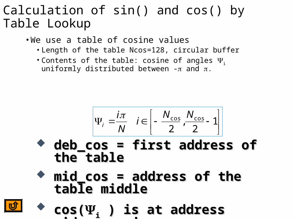
Calculation of sin() and cos() by Table Lookup

• We use a table of cosine values• Length of the table Ncos=128, circular buffer• Contents of the table: cosine of angles i uniformly distributed between -

and . 

1

2,

2coscos NN

iNi

i

deb_cos = first address of the tabledeb_cos = first address of the table mid_cos = address of the table middlemid_cos = address of the table middle cos(cos(ii ) is at address mid_cos + i ) is at address mid_cos + i

Calculation of sin() and cos() by Table Lookup

• Conversion of the phase modulo 2:• Wrapping phase in [-,[ • Done by a macro: testa02pi

* Macro to wrap the phase between - et , phase is in ACCU A testa02pi .macro SUB #8000h,A,B ; sub -2^(15) BC suite1?, BGEQ ; test if phase is in [0,2pi[ SUB #8000h,A ; sub -2^(15) SUB #8000h,A ; SUB -2^(15) B suite? suite1? ADD #8000h,A,B ; add -2^(15) BC suite?,BLT ADD #8000h,A ; add -2^(15) ADD #8000h,A ; add -2^(15) suite? ; end of test .endm

Generating the Sine Values from a Table of Cosine Values

• To generate sin() from the table of cosine values, we use:• cos(/2 - ) or cos(-/2 + ) or cos(3/2+ )• If i is the index of the cosine, for the sine we use:

• i-Ncos/4 if i>= -Ncos/4 • i+3Ncos /4 if i < Ncos/4.

Implementation on a C54x, Test Sequence• We can test the GMSK modulation on a given periodical binary

sequence an:• an=[ 0 1 1 0 0 1 0 1 0 0]• These bits are stored in a circular buffer:

• Size NB = 10• Declaration of a section bits aligned on an address which is a multiple of 16 bits.

AR5 deb_bit

NB

an

Testing the Generation of on the C54x,Results Buffer

• We calculate and store it in a buffer pointed by AR1. The size of the result buffer is 1000 words.

AR1 resu

1000

Buffer for the last 1000 result values of

Testing the Generation of on the C54xBuffers

AR4 phi

Nphi

phi

Circular Buffer for phi (evolutive part) Allocated at an address multiple of 64

(Nphi = 32)

AR3 deb_phase

Nphi

phase

Circular Buffer for the variable phase Allocated at an address multiple of 64

(Nphi = 32)

Listing for the Calculation of Definitions

.mmregs .global debut,boucle .global deb_cos, phi .global deb_phase .global resu

Nphi .set 32 Nphim .set -32 L .set 4 Ncos .set 128 Nsur2 .set 64 Nsur4 .set 32 NB .set 10 NS .set 8

.bss resu,1000

Listing for the Calculation of Macro for phase wrapping

* Definition of macro of phase wrapping testa02pi testa02pi .macro SUB #8000h,A,B ;sub -2^(15)

BC suite1?, BGEQ ;test if phase in [0,2pi[ SUB #8000h,A ;sub -2^(15) SUB #8000h,A ;sub -2^(15) B suite?

suite1? ADD #8000h,A,B ;add -2^(15) BC suite?,BLT ADD #8000h,A ;add -2^(15) ADD #8000h,A ;add -2^(15)

suite? ;end test wrapping [0,2pi[ .endm

Listing for the Calculation of Initialization of Registers and Buffers 1/2

.text * Initialization of BK, DP, ACCUs, and ARi debut: LD #0, DP

LD #0, A LD #0, B STM #deb_bit,AR5 STM #deb_cos,AR2 STM #deb_phase ,AR3 STM #phi,AR4 STM #resu,AR1 STM +1,AR0 STM #Nphi, BK STM #(NS-1),AR7 RSBX OVM SSBX SXM

Listing for the Calculation of Initialization of Registers and Buffers 2/2

* Initialization of the phase buffer RPT #(Nphi-1) STL A,*AR3+%

*initialization of phimem LD *AR5,T MPY #04000h,A ; -2^(14) an(1)(pi/2 an(1)) STL A,*(phimem)

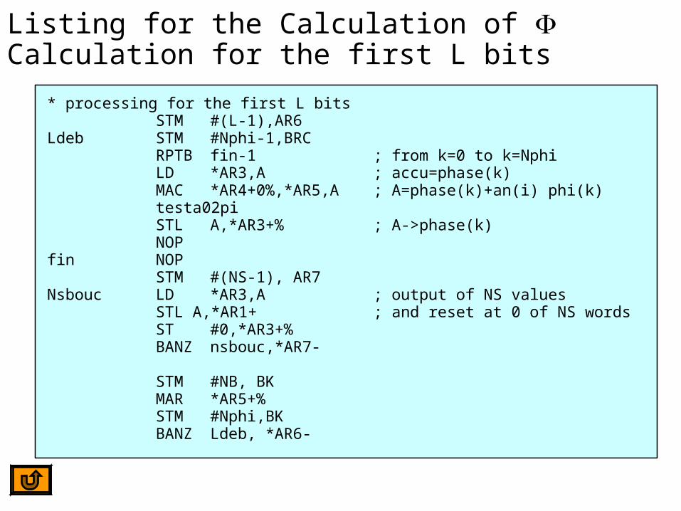
Listing for the Calculation of Calculation for the first L bits

* processing for the first L bits STM #(L-1),AR6 Ldeb STM #Nphi-1,BRC

RPTB fin-1 ; from k=0 to k=Nphi LD *AR3,A ; accu=phase(k) MAC *AR4+0%,*AR5,A ; A=phase(k)+an(i) phi(k) testa02pi STL A,*AR3+% ; A->phase(k) NOP

fin NOP STM #(NS-1), AR7

Nsbouc LD *AR3,A ; output of NS values STL A,*AR1+ ; and reset at 0 of NS words ST #0,*AR3+% BANZ nsbouc,*AR7- STM #NB, BK MAR *AR5+% STM #Nphi,BK BANZ Ldeb, *AR6-

Listing for the Calculation of Calculation of the Following Bits 1/2 * begin of the infinite loop boucle STM #Nphi-1,BRC

RPTB fin2-1 ; for k=0 to Nphi LD *AR3,A ; accu=phase(k) MAC *AR4+0%,*AR5,A ; A=phase(k)+an(i) phi(k) testa02pi STL A,*AR3+% ; A->phase(k)

fin2 * adding phimem to the NS first points of the array * then taking them out and reset to 0 in phase

STM #NS-1,AR7 nsbouc2 LD *(phimem),B

ADD *AR3,B,A ; B=phimem+phase(k) testa02pi STL A,*AR1+ ST #0,*AR3+% ; 0->phase(k) BANZ nsbouc2,*AR7- ; ....

Listing for the Calculation of Calculation of the Following Bits 2/2

fin3 * actualization of phimem

LD *(phimem),A STM #NB, BK MAR *+AR5(#unmL)% LD *AR5,T MAC #04000h,A ; -2^(14) an(1)(pi/2 an(1)) testa02pi STL A,*(phimem) MAR *+AR5(#L)% STM #Nphi,BK B boucle .end

Illustration of the Phase Result Wrapped Between - and

• Plot under CCS the buffer of phase results

Generation of the Baseband ComponentszI=cos() and zQ=sin()

• We calculate zI and zQ and we do not need to save the phase any more.

• We output ZI and Zq, in this example on DXR0 and DXR1.• We need the table of constants for the values of cosine.

• This table is defined in the file tabcos.asm• The cosine values are given in format Q14.

File tabcos.asm

.def deb_cos,mid_cos .sect "tab_cos"

deb_cos .word -16384,-16364,-16305,-16207,-16069,-15893,-15679,-15426 .word -15137,-14811,-14449,-14053,-13623,-13160,-12665,-12140

.word -11585,-11003,-10394,-9760,-9102,-8423,-7723,-7005 .word -6270,-5520,-4756,-3981,-3196,-2404,-1606,-804 .word 0,804,1606,2404,3196,3981,4756,5520 .word 6270,7005,7723,8423,9102,9760,10394,11003 .word 11585,12140,12665,13160,13623,14053,14449,14811 .word 15137,15426,15679,15893,16069,16207,16305,16364 .word 16384,16364,16305,16207,16069,15893,15679,15426 .word 15137,14811,14449,14053,13623,13160,12665,12140 .word 11585,11003,10394,9760,9102,8423,7723,7005 .word 6270,5520,4756,3981,3196,2404,1606,804 .word 0,-804,-1606,-2404,-3196,-3981,-4756,-5520 .word -6270,-7005,-7723,-8423,-9102,-9760,-10394,-11003 .word -11585,-12140,-12665,-13160,-13623,-14053,-14449,-14811 .word -15137,-15426,-15679,-15893,-16069,-16207,-16305,-16364

mid_cos .set deb_cos+64

Listing for the Calculation of zI and zQ• The listing for definitions and initializations is the same as before.• Processing of the L first bits,• Processing of the other bits

• (infinite loop)

Processing of the First L Bits 1/2 * Processing of the L first bits

STM #(L-1),AR6 Ldeb STM #Nphi-1,BRC

RPTB fin-1 ; from k=0 to Nphi LD *AR3,A ; accu=phase(k) MAC *AR4+0%,*AR5,A ; A=phase(k)+an(i) phi(k) testa02pi STL A,*AR3+% ; A->phase(k)

fin NOP STM #(NS-1), AR7

Nsbouc LD *AR3,A ; output of NS values SFTA A,-9,A ADD #mid_cos,A,B STLM B,AR1 NOP NOP LD *AR1,B STL B,DXR0

Processing of the First L Bits 2/2 * Calculation of the sine ADD #Nsur4,A,B BC sui,BGT ADD #(Nsur2),B B sui1

sui SUB #Nsur2,B sui1 ADD #mid_cos,B

STLM B,AR1 NOP NOP LD *AR1,A STL A,DXR1 ST #0,*AR3+% BANZ nsbouc,*AR7- STM #NB, BK MAR *AR5+% STM #Nphi,BK

Processing of the Following bits 1 of 2 * begin the infinite loop boucle STM #Nphi-1,BRC

RPTB fin2-1 ; for k=0 to Nphi LD *AR3,A ; accu=phase(k) MAC *AR4+0%,*AR5,A ; A=phase(k)+an(i) phi(k) testa02pi STL A,*AR3+% ; A->phase(k)

fin2 *phimem is added to the NS first points of the array * then they are output and words are reset to 0 in buffer phase

STM #NS-1,AR7 nsbouc2 LD *(phimem),B

ADD *AR3,B,A ; A=phimem+phase(k) testa02pi SFTA A,-9,A ADD #mid_cos,A,B STLM B,AR1 NOP NOP LD *AR1,B

STL B,DXR0

Processing of the Following Bits 2 of 2

* Calculation of the sine NOP ADD #Nsur4,A,B NOP NOP BC suii,BGT ADD #(Nsur2),B B suii1

suii SUB #(Nsur2) ,B suii1 ADD #mid_cos,B

STLM B,AR1 NOP NOP LD *AR1,A STL A,DXR1 ST #0,*AR3+% ; 0->phase(k) BANZ nsbouc2,*AR7-

fin3 * actualization of phimem

LD *(phimem),A STM #NB, BK MAR *+AR5(#unmL)% LD *AR5,T MAC #04000h,A ; -2^(14) an(1)(pi/2 an(1)) testa02pi STL A,*(phimem) MAR *+AR5(#L)% STM #Nphi,BK B boucle .end

Results Observed in CCS

Generation of 2 Quadrature Carriers• Generation of:• cos(2fct) and sin (2fct)• fc is the frequency of the carrier• In this example we choose fc=1/T• Sampling frequency = 1/Ts = fS

• In RF applications, the carriers are not generated by the DSP. It is only possible to use the DSP for low values of fc.

• The angle (t)= 2fct is calculated then the value of cos() is read from a table.

Calculation of the Angle of the Carriers• Recursive calculation of the angle :

( ) 2 ( 1) 2 ( 1)S c S S c S snT f nT n T f T n T

The precision of the generated The precision of the generated frequency depends on the precision of frequency depends on the precision of ..

The phase increment The phase increment corresponds to corresponds to an increment an increment II to the integer that to the integer that represents represents ..II=2=21616ffccTTSS rounded to the closest rounded to the closest

integer.integer.

Calculation of the Angle of the Carriers• If the number of samples per period of the carrier is a power of 2,

2k:

•I=216fcTS=2(16-k) is exact•Then the precision of the generated frequency depends only on the precision of the sampling frequency.

• Otherwise, there is an error dfc in fc:• |dfc|<2-17fS.

• Error in the amplitudes of the carriers due to finite precision of the table reading. (possible interpolation).

Implementation on a C54x• We use: fs/fc=8=Ns.• The cosine table has 128 Values in Q14.

AR1 deb_cos

128 Cosine values

Circular buffer,Table of cosine

Implementation on a C54x• Here k=3 (8 samples per period) and the increment

• I=216fcTS=2(16-k) =213

• Simple case of fS/fc as an integer value, the table is read with an offset from the pointer = 16 = 27/23 to generate a cosine with 8 samples per period.

• We can work directly on the index i and not on I.

Generation of the Cosine and Sine Carriers• For the cosine:

• The circular buffer containing the cosine values (length N) is accessed with AR1.

• Incremented by the content of AR0=16.• AR1 initialized with deb_cos.

• For the sine:• Same circular buffer accessed by AR2.• AR2 initialized with deb_cos + Ncos/4.• Decremented by AR0=16.

• Outputs (cos and sin) are sent to DXR0 and DXR1.

Generation of quadrature 2 Carriers• File porteuse.asm• A file associated with DXR0 and DXR1 is used to save visual results

obtained with the CCS simulator.• Here cosine table goes from:

• 0 to 2

Listing for the Generation of 2 Carriers 1 of 2

.mmregs

.global debut,boucle Ncos .set 128 Nsur2 .set 64 Nsur4 .set 32 Inc .set 16 * Definition and initialization of Table of cosine

.sect "tab_cos" deb_cos .word 16384,16364,16305,16207,16069,15893,15679,15426

.word 15137,14811,14449,14053,13623,13160,12665,12140 .word 11585,11003,10394,9760,9102,8423,7723,7005 .word 6270,5520,4756,3981,3196,2404,1606,804 .word 0,-804,-1606,-2404,-3196,-3981,-4756,-5520 .word -6270,-7005,-7723,-8423,-9102,-9760,-10394,-11003 .word -11585,-12140,-12665,-13160,-13623,-14053,-14449,-14811 .word -15137,-15426,-15679,-15893,-16069,-16207,-16305,-16364 .word -16384,-16364,-16305,-16207,-16069,-15893,-15679,-15426 .word -15137,-14811,-14449,-14053,-13623,-13160,-12665,-12140 .word -11585,-11003,-10394,-9760,-9102,-8423,-7723,-7005 .word -6270,-5520,-4756,-3981,-3196,-2404,-1606,-804 .word 0,804,1606,2404,3196,3981,4756,5520 .word 6270,7005,7723,8423,9102,9760,10394,11003 .word 11585,12140,12665,13160,13623,14053,14449,14811 .word 15137,15426,15679,15893,16069,16207,16305,16364

Listing for the Generation of 2 Carriers 2 of 2 .text * Initializations of DP, and of the phase Ialpha at 0 * The phase Ialpha is in ACCU A, and the index of table in B * attention we work in the part of ACCUs * Initialize AR1 at mid_cos and AR0 at Nsur4 debut:

LD #0, DP LD #0, A STM #Ncos,BK STM #deb_cos,AR1 STM #(deb_cos+Nsur4),AR2 STM #Inc, AR0

* endless loop boucle:

LD *AR1+0%,A STL A, DXR0 LD *AR2-0%,B STL B,DXR0

* Return to the beginning of the endless loop B boucle

Results Obtained with CCS

Tutorial The listing files for the precedent examples The listing files for the precedent examples can be found in the directory “tutorial”:can be found in the directory “tutorial”: Tutorial > Dsk5416 > Chapter 21 > Labs_modulationTutorial > Dsk5416 > Chapter 21 > Labs_modulation

Further Activities• Application 5 for the TMS320C5416 DSK and for the TMS320C5510. • Alien Voices. A very simple application showing the effect

of modulation on audio frequencies. It shows how the carrier causes sum and difference frequencies to be generated. Here it is used to generate the strange voices used for aliens in science fiction films and television.