frequency modulation · transmitters for frequency modulation 226 43. fm transmitters. -44. the...
TRANSCRIPT

RADIO COMMUNICATION SERIES BEVERLY DUDLEY, CONSULTING EDITOR
FREQUENCY MODULATION
www.americanradiohistory.com


FRF:QUENCY IO D ULATT ON
BY
AUGUST HUND Technical Consultant, U. S. Navy Radio and Sound Laboratory,
San Diego, California
FIRST EDITION FOURTH IMPRESSION
McGRAW -HILL BOOK COMPANY, INC.
NEW YORK AND LONDON 1942
www.americanradiohistory.com

FREQUENCY MODULATION
COPYRIGHT, 1942, BY THE
MCGRAW -HILL BOOK COMPANY, INC.
PRINTED IN THE UNITED STATES OF AMERICA
All rights reserved. This book, or parts thereof, may not be reproduced in any form without permission of
the publishers.
THE MAPLE PRESS COMPANY, YORK, PA.
www.americanradiohistory.com

PREFACE
The purpose of this book is to present an engineering text on frequency modulation covering both basic principles and the design of commercial apparatus. The practical applications that are described follow closely good present -day engineering practice.
Frequency modulation is a new development in the art of radio, and short cuts should be used only when the features that frequency modula- tion stands for are not violated. The main features are high -fidelity transmission and a modulation system that avoids some of the interference otherwise occurring in the transmission by means of carrier currents.
A thorough knowledge of the principles underlying frequency modu- lation is essential to an appreciation of the design necessary for the apparatus.
It has been necessary to make use of Bessel functions and customary calculus, but the reader will find that the engineering applications are simple, especially when the curves and tables given in this book are used. Some of the tables and curves show at a glance the band width required for transfer networks. The applications presented can be understood without a knowledge of the derivations. Detailed numerical computa- tions appear throughout the text and in connection with design formulas. Numerical calculations often appear step by step so that the reader not well versed in such applications should have no difficulty in understand- ing how to obtain a design value. To some readers such a treatment may look tiresome and lacking in unity. It should be understood, how- ever, that the unity of the presentation lies in the method of approach in the mathematical and numerical formulation of problems that occur in the branch of FM engineering.
It has also seemed necessary to use often abbreviations such as FM, PM, and AM instead of the long expressions frequency modulation, phase modulation, and amplitude modulation. It is admitted that such abbreviations have a certain degree of abruptness, especially when used as nouns. The reader will find, however, that sentences often appear much Iess involved when the abbreviations are used. This is a text on a new phase of radio engineering and many novel phenomena are explained and abbreviations for expressions that occur often can, therefore, be excused when, by their use, the remainder of a sentence becomes more prominent.
It has seemed advisable to describe phenomena and features in fre- quency modulation as compared with customary amplitude modulation
v
www.americanradiohistory.com

vi PREFACE
and phase modulation. The latter type of modulation is by no means the same as frequency modulation although some similarities exist. Because of this comparison, the text is also a book on the basic princi- ples of all three types of modulations.
Simultaneous occurrence of frequency modulation with either of the two other types of modulation, as well as the simultaneous action of all three types of modulation, is treated in the theoretical part of the book. This is done in order to show that an amplitude limiter can be used suc- cessfully and without producing distortion only when amplitude vari- ations are not caused in the primary frequency -modulation stage by the same stimulus that causes the desired frequency modulation. Besides, the theory of the superposition of different types of modulations may be thought- provoking about other applications not yet in use.
The text is divided into five chapters and an Appendix. The first chapter deals with fundamental relations. It discusses noise interference and wave propagation in the upper megacycle range of carrier frequencies, which are of concern in FM systems. It will be found that the field intensity now decreases with the square of the distance to the transmitter and that we deal essentially with only a primary service area. Since many principles are discussed in this chapter, much space had to be devoted to it.
Chapter II deals with auxiliary apparatus such as frequency modu- lators, frequency discriminators, and amplitude limiters. Much stress has been put upon showing that the speed of electrical actions in net- works, partly due to their circuit elements, plays an important part in the best design of apparatus. For this reason a section on time constants was added in this chapter. In the section on amplitude limiters, as well as in the section on preaccentuators and deaccentuators, it is brought out how such apparatus are to be designed with respect to suitable time con- stants. This feature can also be noted in Figs. 80 and 85, which show apparatus used in FM receivers. In FM systems the linear tube require- ments are of secondary importance, but the networks between tubes have to be linear with respect to amplitude as well as phase for the entire range of carrier frequencies belonging to the particular band width.
Chapter III gives descriptions of all commercial FM transmitters manufactured in this country. The descriptions are presented in con- junction with the results found in Chap. I.
Chapter IV gives a detailed description of FM receivers. A designer should have no difficulty in applying the given networks to his particular needs. Many receiver tests are also described in this chapter.
Chapter V deals with receiver and transmitter aerials as well as with feeders such as are being used in the range of frequencies assigned to FM stations.
www.americanradiohistory.com

PREFACE vii
The Appendix gives a detailed solution for the distribution of the modulation energy in the frequency spectrum. It is the width occupied by the significant side currents in this spectrum for which the transfer networks have to be designed and not necessarily the peak -to -peak frequency swing. The Appendix gives also tables for the integral -sine,
cosine, and exponential functions that are so useful in computing the reactance and resistance components of high -frequency conductors. The simple numerical application of such tables and corresponding curves like-
wise given in this book is described in detail in Chap. Y. There is also
added a table for circular, hyperbolic, and exponential functions in terms of increasing arguments expressed in radians. The corresponding angle
in degrees is added in these tables in order to have a comparison for
circular functions. To express such functions in terms of radian units especially useful in engineering solutions occurring in FM problems, since
the modulation index, which is the ratio of the amplitude frequency swing
to the signal frequency, is numerical. The references at the end of the Appendix cover most of the current literature and are intended for readers who wish to follow up certain phases of FM engineering.
The features of this book are, therefore: 1. The text is useful for the practicing engineer as well as for class-
room work. 2. A critical treatment of nearly every phase encountered in present -
day FM engineering is presented. 3. The text is complete in itself. 4. All theoretical derivations are applied to present -day FM apparatus. 5. Numerically and in gradual steps, it is demonstrated how appar-
ently difficult mathematical formulas can be readily applied to engineer- ing solutions, by the use of either tables or curves.
6. Many explanations are given directly in the illustrations o that the figures can often be used without consulting the text.
7. The treatment is thorough and should, therefore, also be of use to the expert in the field of FM engineering.
8. Inasmuch as special design formulas often have to be employed in
connection with band width and the natural speeds of networks, this text helps to bring the information on circuit design up to date.
9. The importance of servicing and maintaining FM receivers has been recognized by the inclusion of text material on useful tests and com- plete alignment of FM receivers.
10. Inasmuch as Chap. I presents a general theoretical treatment of
amplitude, phase, and frequency modulation, this book furnishes a com- parison and evaluation of the three methods of modulation.
The author is much indebted to the publishers and their editorial staff, who have encouraged such a publication from the very beginning
www.americanradiohistory.com

viii PREFACE
and made invaluable suggestions while the manuscript was being pre- pared. The author is indebted to Mr. O. L. Heeger, of the Radio Institute of California, under whose auspices lectures on frequency modulation were given by the author to a group of broadcast engineers. This enabled the author to find out what is actually needed in the pres- entation of such a publication. Credit is also due Mr. Clyde W. Tirrell, Navy Radio and Sound Laboratory, San Diego, Calif., who has read the manuscript twice with respect to exposition.
The author welcomes any corrections or suggestions for improvement.
AUGUST HUNA. Santa Monica, Calif.,
October, 1942.
www.americanradiohistory.com

CONTENTS PAGE
PREFACE V
CHAPTER I
FUNDAMENTAL RELATIONS AND FEATURES IN FREQUENCY -MODULATED, PHASE -
MODULATED, AND AMPLITUDE- MODULATED SYSTEMS 1
1. Fundamental Relations. -2. Basic Relations and Features for Amplitude
Modulation. -3. Fundamental Relations and Features for Phase Modu-
lation.-4. Relations and Features for Frequency Modulation. -5. Side -
current Distribution in Frequency Modulation and Phase Modulation. - 6. Application of Bessel Tables and Bessel Curves. -7. Numerical Specula-
tions on Frequency Swing, Equivalent Phase Swing, and Band Width. - 8. Useful Formulas for Small Modulation Index. -9. Three Types of
Modulation. -10. Addition of Modulation Products. -11. Effects When
Two Types of Modulations Are Present. -12. Effects When Frequency
Modulation and Amplitude Modulation Are Present. -13. Actions in
Threefold Modulation (FM + PM + AM).-14. Translation of Signal
Currents into Corresponding Frequency and Phase Variations. -15. Trans-
lation of Frequency Modulation and Phase Modulation into Amplitude
Modulation. -16. Determination of Maximum Frequency and Maximum
Phase Deviations and of the Mean Carrier Frequency. -17. Effect of Band
Restriction Filters on Currents Modulated in Frequency. -18. Interference and Its Partial Elimination in FM Systems. -19. Phase Modulation,
Equivalent Frequency Modulation, and Amplitude Effect of Two Received
Carrier Currents. -20. Superposition of Currents in Transfer Networks. - 21. Different Kinds of Interference Impulses. -22. Frequency Multiplication
in FM Systems. -23. Frequency Division in FM Systems. 24. Heterodyn-
ing in FM Systems. -25. Wave Propagation in the Present -day FM Band
CHAPTER II
AUXILIARY APPARATUS EMPLOYED IN FM SYSTEMS 150
26. Balanced Modulators. -27. Ring Modulators. -28. Frequency Divi-
sion by Regenerative Modulation. -29. Reactance Tubes. -30. Design
Formulas and Useful Quadrature Tube Modulators. -31. Frequency
Modulators. -32. Balancing of a Two -tube Frequency Modulator. -33. Phase Modulators. -34. Commerical Demodulators. -35. Actions in Fre-
quency Discriminators. -36. Band -width Design of Discriminators. -37. Useful Discriminator Networks. -38. Tests on Descriminators. -39. Useful
Amplitude Limiters. -40. Time Constants in FM- Networks. -41. Networks
for Audio -frequency Accentuation and Deaccentuation. -42. Networks for
Producing Inverse Frequency Effects.
CHAPTER III TRANSMITTERS FOR FREQUENCY MODULATION 226
43. FM Transmitters. -44. The Armstrong Indirect FM Transmitter.- 45. The FM Transmitter of the General Electric Company. -46. The
ix
www.americanradiohistory.com

CONTENTS PAGE
FM Transmitter of the Radio Corporation of America. -47. The FM Transmitter of the Western Electric Company. -48. Notes on FM Signal Generators.
CHAPTER IV RECEIVERS FOR FREQUENCY- MODULATED CURRENTS 249
49. FM Receivers. -50. Typical Sections in an FM Receiver. -51. Characteristic Curves in FM Receivers. -52. Image Response in FM Sys- tems in Comparison with Such Responses in AM Systems. -53. All Net- works in an FM Receiver. -54. Alignment of FM Receivers.
CHAPTER V
TRANSMITTER AND RECEIVER AERIALS 278
55. Radiation of Waves in the Carrier Frequency Spectrum of FM Waves. - 56. Input Impedance and Mutual Impedance of Dipoles. -57. FM Voltage Effective at the Input Terminals of an FM Receiver in Terms of the Electric Field Intensity. -58. Effect of the Q Value of Linear Conductors on the Self - impedance.-59. Dipoles for FM Reception. -60. Dipoles with a Reflector. -61. Feeders Used in FM Systems. -62. Formulas and Computations for Feeders and Matching Sections. -63. Feeder Tests. -64. Linear Conductors Used as Radiators. -65. Excitation of Dipoles. -66. Transmitter Antennas. -67. Quarter- wave -length Feeder Sections.
APPENDIX 347
68. Theory of the Spectrum Solution. -69. Effective Input Impedance and Q Value of Feeders. -70. Magnitudes of Important Factors. References.
INDEX 367
www.americanradiohistory.com

FREQUENCY MODULATION In commercial alternating- current technique, distortion in a current is
generally considered an undesirable by- product. In communication engi-
neering even pronounced linear distortion is often desirable since it can be
used for transmitting intelligence, as is described in this volume. In pure mathematics, certain functions lead to an infinite series of
terms, which often do not yield a very useful solution. In this volume,
Bessel and other functions are made use of and yield convenient design
formulas for computing the band width and other circuit properties in com-
munication systems employing phase or frequency modulation.
CHAPTER I
FUNDAMENTAL RELATIONS AND FEATURES IN FREQUENCY -MODULATED, PHASE -MODULATED,
AND AMPLITUDE -MODULATED SYSTEMS
Inasmuch as a high- frequency (h -f) current is characterized by its amplitude, frequency, and phase, it can be distorted or modu- lated by amplitude changes, by frequency changes, or by phase changes. We can; therefore, have amplitude modulation (AM),
frequency modulation (FM), and phase modulation (PM). It is also possible that any two of these modulations may exist
simultaneously or that all three types may occur. With present - day commercial practice only one kind of modulation, say FM, is desirable in a given system. The other two, if they exist
simultaneously, are undesirable by- products. A clear understanding of all three types of modulation is
necessary in order to account for undesirable superimposed modula-
tions of either of the two undesired types. A clear understanding is also essential since, besides direct FM systems, we have a com-
mercial transmitter system where AM produces the first side -
pair modulation product. In virtue of the action of certain
circuit elements, this gives rise to PM effects, and in virtue of the further action of another correcting network gives a frequency spectrum distribution as though FM were the cause. This has
reference to the well -known Armstrong system of frequency modulation.
1
www.americanradiohistory.com

2 FREQUENCY MODULATION [CHAP. I
1. Fundamental Relations. -The general equation' for the instantaneous value It of an unmodulated sinusoidal carrier cur- rent, as shown in Fig. 1, is
It = Im sin a = Im sin (1.2t + 0) (1)
This represents a vector of constant length Im rotating in a counter- clockwise direction with a constant angular velocity 12. We note that, in the general case, we have a fixed relative phase 0. Now,
1t
2 seconds 12
12=27F 1 F carrier frequent
11Th
t seconds
FIG. 1.- Current wave of amplitude I,,,, period 1/F seconds and relative phase 8.
if a signal current of instantaneous value it = im cos wt is acting on a suitable modulator, we can affect the carrier amplitude Im without varying either 12 or 0, thus producing AM. And if Im and E2 are kept constant, so that the signal current varies only the relative carrier phase 0 with maximum phase deviations or phase swings of ±00, we have PM. If Im and O are kept constant and only the carrier frequency F, in 12 = 6.28F, is varied by means of the signal current with maximum frequency deviations or fre- quency swings of ±OF, we have FM.
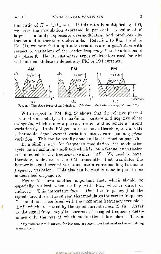
Referring to Fig. 2a, we note that for sinusoidal AM the carrier amplitude or carrier level Im fluctuates periodically between the limits Im -im and Im + im; i.e., the maximum carrier level deviations are ±im as is well known in the art. Full or 100 per cent modulation occurs when the amplitude im of the signal current, so to speak, "uses up" the entire carrier level Im as the modulation takes place downward. This occurs for Im = im or for a modula-
i Inasmuch as in current literature on FM several different symbols are in use for the same quantities, the nomenclature adopted in this book is that used in "High - frequency Measurements," McGraw -Hill Book Company, Inc., New York. F stands for the carrier frequency since it is always larger than the frequency f of the modulating or signal current. Any measurable deviations from the carrier frequency F are denoted by oF. We then have S2 = 21rF; w = 2,rf; and M1 = 2r F. This procedure seems logical and gives expressions that are clearer to the eye than subletters.
www.americanradiohistory.com
SEC. 11 FUNDAMENTAL RELATIONS 3
tion ratio of K = iL /I,,, = 1. If this ratio is multiplied by 100,
we have the modulation expressed in per cent. A value of K larger than unity represents overmodulation and produces dis- tortion and is therefore undesirable. Referring to Fig. 1 and to Eq. (1), we note that amplitude variations are in quadrature with respect to variations of the carrier frequency F and variations of
the phase O. Hence, customary types of detectors used for AM will not demodulate or detect any FM or PM currents.
et PM
rfsec.1
i. 1aB
(u) t (b)
t (c) t,seconds
Fia. 2. -The three types of modulation. (Maximum deviations are i,,,, AO, and ¿F.)
With respect to PM, Fig. 2b shows that the relative phase O
is varied sinusoidally with matimum positive and negative phase swings AB, which is now a phase variation and no longer a current variation iL. In the PM generator we have, therefore, to translate a harmonic signal current variation into a corresponding phase variation. This can be readily done and is described on page 75.
In a similar way, for frequency modulation, the modulation cycle has a maximum amplitude which is now a frequency variation and is equal to the frequency swings ±OF'. We need to have, therefore, a device in the FM transmitter that translates the harmonic signal current variation into a corresponding harmonic frequency variation. This also can be readily done in practice as is described on page 75.
Figure 2 shows another important fact, which should be especially realized when dealing with FM, whether direct or
indirect.' This important fact is that the frequency f of the signal current, i.e., the current that modulates the carrier frequency F, should not be confused with the maximum frequency excursions ±OF, which are caused by the signal current im cos (2irf)t. As far as the signal frequency f is concerned, the signal frequency deter- mines only the rate at which modulation takes place. This is
1 By indirect FM is meant, for instance, a system like that used in the Armstrong
transmitter.
www.americanradiohistory.com

6 FREQUENCY MODULATION [CHAP. I
the vector OP to a length OP1. Then OP1 rotates at this instant
with the unchanged angular velocity 27rF since F is fixed for AM.
Now, if a phase -shifting network causes PP' = im to act perpen-
dicularly, as in Fig. 3b, with the vector OP, then the resultant
instantaneous vector OP1 is no longer in phase with the unmodu-
lated carrier level OP but is deviated by an angle 09 from the
inphase position. If the modulating vector had been -im, the
resultant vector would have been OP2 in Fig. 3b, of same length
im K= Im OP= Im sin lit PP, = (imsin cvt)siniLt
P --- ?2=11tF
z P
AM
m
Im
OPI= Im JtK2sin2wt sin ̀ ittttañ
=Im 1+K2sin2wt sin nt+Ksincut/
nt OP=Imsinflt p PP = (im sin cut)cosllt de=K
LIB im (cos llt sin cvt) -
=2iesin(Il-rw)t -Zimsin(1l-cv)t 0
P
114- CO
PM
(a) (b)
FIG. 3.- Addition of carrier frequency component and modulation product.
as OP1, but the angular shift AO would be in the other direction
from OP. This is what occurs when the signal- current amplitude
swings from +im to -im; i.e., when 27rft changes from 0 to 180
deg of the signal cycle. Hence, we obtain a PM with a peak -to-
peak phase swing of 2 M. Therefore, the instantaneous angular
velocity Ste is generally not equal to St = 27rF except at the moments
of maximum phase deviation indicated in Fig. 3b. This means
that in effect we have also "equivalent" FM since Sty can differ
from St only when F undergoes equivalent variations. Figure 3b indicates also the degree of PM since M denotes the
maximum phase excursion and is equal to tan-1- (PP1 /0P). For
instance, for a ratio of the quadrature components of 0.5, we have
approximately M = 0.5 radian, or 57.3 X 0.5 = 28.65 deg. With
respect to the ratio PP1 /OP, which determines the maximum phase
swing M, it should be understood that absolute linearity (no
distortion) can exist only when this ratio is equal to the angle in
www.americanradiohistory.com

SEC. 2J FUNDAMENTAL RELATIONS 7
radians. This is strictly true only for small arguments of the tangent function, such as 0.2 and smaller. This is the reason why in many practical applications in this text 0.2 is assumed as
the upper limit. Without resorting to the analysis for the 0.2 con-
dition, we note by inspecting Fig. 3b that only for short lengths of
PP, can we expect a PM with the entire length PP, as a portion of a circle. If we have no true circle, then we have radius vectors of different lengths instead of constant OP values. This means we have also a certain amount of AM. Nevertheless, in practical' indirect FM work angles2 not exceeding 0.5 radian or 28.65
(roughly 30 deg) are made use of. Moreover, it should be noted that the length of vector OPl shown in Fig. 3b changes somewhat for such an upper limit as ±30 deg and causes a small degree of
AM, the effects of which can be avoided by means of an amplitude limiter.
Generally, the modulation vector PP, in Fig. 3b can make any angle differing from 90 time degrees, except 0 or 180 deg, with respect to the vector OP representing the unmodulated carrier level and still leave components that account for PM and equiva- lent FM effects. But for such conditions we shall also experience more or less pronounced AM. A system of this type may some
day have values, though in present -day work where amplitude limitation is partly responsible for good FM reception, such vec- torial addition of the modulation product is not advisable, nor is
it efficient. 2. Basic Relations and Features for Amplitude Modulation. -
Since with AM only the carrier level varies, i.e., the amplitude I. in Eq. (1), we have for the instantaneous carrier level for K = im /Im; the relation Imt = K cos wt). This is illustrated in3
l Indirect FM should not be confused with equivalent FM. In indirect FM we
have exactly the same frequency spectrum distribution as in direct FM, and hence all
the features inherent with direct FM. In other words a receiver would not disclose
whether the received wave comes from an Armstrong transmitter using indirect FM or from a direct FM system. This assumes that frequencies below 50 cycles are of
no great interest as far as full modulation is concerned. For equivalent FM the spectrum distribution holding for PM prevails.
a Such large upper limits produce about 10 per cent harmonic distortion. Accord- ing to Eq. (6) we have f AB for the equivalent carrier -frequency change.
' Figure 4 shows the case for Im(1 -J- K sin wt) sin Sgt in order to show also equations for a sinusoidal amplitude variation. If only AM is of interest, cosinoidal and sinusoidal amplitude effects lead to the same result, as far as the frequency spectrum is concerned.
www.americanradiohistory.com

8 FREQUENCY MODULATION [CHAP. I
Fig. 4. If the constant relative phase O is ignored and the instan- taneous amplitude Imt is used instead of Im in Eq. (1), there results
It = Imt sin 52t = Im(1 -{- K cos wt) sin IN modulation product
= Im sin Sgt -{- (KIm cos wt) sin Sgt
a (2)
showing that portion a is the original unmodulated carrier of
level Im and that portion b is the modulation product. It is this
4,4 & sin wt =/m (lfKs /n wt)
k
1 Imsinl2t + /ms /nAts /n cut =lf%
Unmodulated Completely high frequency modulated h /qh (carrier)current frequency current
FIG. 4.- Amplitude modulation of a high- frequency current of carrier frequency 12/27r by means of a signal current of frequency w /27r.
product which, so to speak, "handles" the signal or modulation energy. Hence, with AM the modulation energy is entirely in the side bands. The expansion of portion b yields
b = 0.5KIm {sin [271- (F -{- f)t] + sin [27r. (F - f)t] } (3)
It is this product that is produced at the output of a balanced amplitude modulator since the carrier portion a is balanced out or suppressed in such a modulator.
Inasmuch as the output power is proportional to the square of
the respective amplitudes, we learn from Eqs. (2) and (3) and Fig. 5 that in AM for any degree of modulation K, the carrier amplitude Im of the carrier frequency F is preserved unchanged. The entire modulation energy is added in the side bands only. Matters are entirely different for FM where it can even happen that the amplitude of the carrier frequency F disappears entirely or that a certain side -band pair or several of them completely vanish. Another important fact with AM is that in Eq. (2)
1-
t.
\\' K=
rm
%m
Z7r w
www.americanradiohistory.com

SEC. 3] FUNDAMENTAL RELATIONS 9
the term a and the modulation product are in phase with each other since both terms are governed by one and the same sine function, namely, sin Sgt. Another important feature with AM is that the evaluation of the modulation product b in Eq. (3)
into two components of frequencies F -f and F -- f, respectively, shows that the lower as well as the upper side currents both have positive signs before the sine function. If these side currents are compared with the first side- current pair for FM (consult page 39), this will lead to a method by means of which the degree of
FM can be found experimentally with the aid of a superimposed
0.5KIm 0.5KIm
F F -f F F +f FIG. 5.- Carrier frequency amplitude I,,, and respective side- frequency amplitudes 0.5KI,,,.
known AM. Furthermore, it gives a means for finding experi- mentally whether only true FM prevails or whether undesired AM also exists and to what extent it plays a part.
3. Fundamental Relations and Features for Phase Modulation. With PM the carrier level It, as well as the frequency F = S2/6.28
of Eq. (1), remains constant, but the relative phase O undergoes changes. Hence O is no longer fixed, but we have to deal with an instantaneous value Bo, which, according to Fig. 2, for sinusoidal deviations is Bt = O -I- AO sin wt. Since in this case the maximum - phase off swing ±AB corresponds to the amplitude ±im in case of
AM, we can refer it to the original phase O or phase level of the unmodulated carrier, just as im was referred to the original carrier level Im by means of the factor K = im /Im. Doing this with PM, we can represent the ratio OB /B by the degree of modulation factor K2. The factor K2 indicates to what extent and portion of O the phase is periodically advanced and retarded during the signal cycle of frequency f. Unlike the AM case, the phase degree factor K,, can be larger than unity. As a matter of fact, hundreds and even thousands of degrees of maximum phase excursions or phase deviations AO are desirable, especially if we think in terms of
www.americanradiohistory.com

10 FREQUENCY MODULATION [CHAP. I
equivalent wide -band FM. This is important since, as we shall learn later on, periodic and other phase variations can be translated into equivalent frequency variations.
Using the factor KP in the expression for the instantaneous phase, we have
at = B l 1 - AO sin cot) = 0(1 + KP sin wt) (4)
At this point it is stressed that the fixed relative phase 0 in Eq. (1) as well as in Eq. (4) is only a reference datum; i.e., it, has nothing to do with phase modulation. This will be readily understood from the following numerical case. Suppose 0 is 30 deg. Assume that the periodic maximum off swings or phase deviations are AO = +40 deg. Hence, the carrier phase advances once during the signal cycle of frequency f an angular distance of 40 deg and retards during the same signal cycle to the other extreme position of minus 40 deg with respect to the fixed phase O of the unmodulated carrier. It is, therefore, only the variable phase excursions that bring about PM. Now, suppose that the maximum phase devia- tion is still ±40 deg, but that O or the fixed relative phase is 90 deg. Then the unmodulated carrier has the form IL(sin Sgt + 90 °) or Im cos Sgt. This means only that the unmodulated carrier current indicated in Fig. 1 starts with maximum amplitude Im, instead of with the much smaller instantaneous value It as indicated in the figure. This assumed carrier current is, therefore, only a cosine current as far as the reference ordinate axis is concerned. It is still of the same fundamental wave shape. Generally, modula- tions with such slow variations as correspond to audio frequencies will include very many cycles of the high- frequency current which is modulated. Hence, if this so- called "cosine wave" is phase modulated by means of a maximum sinusoidal deviation of ± 40 deg, the same degree of PM must occur as above. For this reason, it is correct to assume that, as far as PM is concerned; the value of O in Eq. (1) stands only for the variable portion of the phase. Then we have for PM the formula for the instantaneous value of the modulated carrier current
It = IP = Im sin (12t + M sin wt) = Im sin a (5)
where it must be realized that only the second term M sin wt
in the expression for a brings about modulation. The term 12 = 27rF is not changed in the case of PM.
www.americanradiohistory.com

SEC. 3] FUNDAMENTAL RELATIONS 11
Nevertheless, something happens in regard to the instantaneous value of the equivalent frequency. This will become clear if we
realize that Im sin a is still a vector of constant length equal to the unmodulated carrier level Im. It still rotates in the conven- tional counterclockwise direction. However, as it tries to rotate with the constant angular velocity SZ = 6.28F, the phase advances and retards or, so to speak, "flutters" forward and backward within the maximum deviation limits of ±M, which for the fore- going numerical example would be ± 40 deg. If these phase deviations swing through an angular distance of ± 360 deg in 1/f sec, we should "wobble" over ± 1 cycle around the true carrier frequency F. There would be, therefore, a gain of 1 cycle and a loss of 1 cycle and the net effect would still be F cycles per second as far as the carrier frequency F is concerned. Hence, the mean carrier frequency or the complete number of carrier cycles during complete signal -cycle periods, referred to a time interval of 1 sec, remains the same. However, the equivalent instantaneous fre- quency Ft of the modulated carrier current does not remain the same in the case of PM.
The value of a includes the phase flutter and denotes the arc in radians or the corresponding angle in degrees through which the rotating vector Im moves in t sec. Therefore da /dt must be the instantaneous angular velocity SZt = 27rFt and 12t /(27r) must be the apparent instantaneous frequency Ft due to PM and due to the fixed frequency F. This yields
Ft = 2r dt = 2 + 2 cos wt
= F f OB cos wt (6) change in instantaneous
frequency due to PM
Figure 6 illustrates what occurs in PM. The line OA denotes the position of the unmodulated carrier current vector of length Im. If sinusoidal PM prevails, this vector flutters or oscillates about the mean position OA located midway between the extreme positions OB and OC. At the same time the entire XY coordinate system spins counterclockwise with the constant angular velocity S2 = 6.28F. As already discussed, the symbol F in the expression SZ = 6.28F stands for the center or mean carrier frequency; i.e., it stands for the number of carrier frequency cycles for one corn-
www.americanradiohistory.com

12 FREQUENCY MODULATION [CHAP. I
plete signal frequency cycle when referred to a time interval of 1 sec. Since, according to Fig. 2, sinusoidal M deviations prevail, the vector OA moves toward the OB position at a rate determined by the signal frequency f. At the extreme position OB the vector must stand still, at least for an instant. The vector immediately afterwards starts to retard its phase; i.e., it starts moving clock-
wise with respect to the uni- formly rotating reference axis after having moved counterclock- B, wise just before reaching the extreme position OB. Hence, the extreme position OB is a position where no phase modulation takes place at all and the true carrier frequency F must prevail at that
x instant. The vector OB moves then clockwise over the original position OA and toward the other extreme, which is position OC.
When reaching this position, the vector has to change over to a counterclockwise rotation. Hence, the true carrier frequency F must also exist for position OC.
The fastest change in the speed of the vector during this phase flutter must, therefore, occur at the position OA, which would be the correct position for the carrier frequency vector if no PM existed. It is the change in this rotational speed that accounts for the equivalent instantaneous carrier frequency change. In Eq. (6) the change f OB cos (2irf)t is caused by the time rate da /dt; i.e., it is caused by the apparent angular velocity of the resultant rota- tion. By resultant rotation is meant the rotation of the X Y coordinate system with constant angular velocity S2 plus the phase- flutter effect. Hence, we must have alternately instan- taneous frequency maxima and minima in the position OA since the oscillation of the vector about the mean position OA due to PM causes the instantaneous equivalent carrier frequency to increase and decrease. It is important to realize that, on account of the time rate da /dt, a sinusoidal, PM causes a cosinoidal equiva- lent FM. These sinusoidal and cosinoidal functions have similar shapes but different amplitudes. However, the shape similarity does not hold at all when rectanguler, triangular, or other wave
Y
FIG. 6.-0 is fixed relative phase and OB maximum phase swing.
www.americanradiohistory.com

SEC. 3] FUNDAMENTAL RELATIONS 13
shapes bring about modulation. Figure 7 shows this for the case where triangular phase swings cause PM. Along the ascending portion 1 -2 of the phase deviation display, the time rate of the phase excursion is constant. Therefore, the equivalent frequency excursion OF, i.e., the instantaneous frequency deviation from the true carrier frequency F, must also be constant and along the horizontal flat top 1 -2 in the derived AF characteristic. All other portions of the derived AF performance are then self- evident.1
Equivalent FM d
dt I 2 3 4 5
Time
-ae
Flo. 7. -Phase and equivalent frequency variations.
The statement just made about wave shapes for sinusoidal PM entails another important fact, which is brought out in Eq. (6). It will be noted that the variable portion in the instantaneous modulated carrier frequency Ft, due to sinusoidal PM, is dependent not only on the maximum phase deviation AO, which causes equivalent FM, but also on the signal frequency f. This equation shows that for signal frequencies of higher pitch, the equivalent frequency shift is larger than it is for frequencies of lower pitch, since the maximum frequency shift is +f AO. That such a condi- tion must exist can be noted directly from Fig. 6. For larger values of the signal or modulating frequency f, the speed of the phase flutter from A to B, back over A to C, forward again to B,
'For other illustrations consult "High- frequency Measurements," pp. 369, 373; "Phenomena in High -frequency Systems," p. 148, McGraw -Hill Book Company, Inc., New York.
www.americanradiohistory.com

14 FREQUENCY MODULATION [CHAP. I
and backward to C, etc., is larger than for smaller values of f. This states that for a fixed maximum phase swing + O, more equivalent FM occurs for audio frequencies of higher pitch.
4. Relations and Features for Frequency Modulation. -In FM systems, modulation is brought about by changing the carrier frequency F in the term S2 = 6.28F of Eq. (1). This means that the carrier level Im and the phase O are kept constant. Since in Sec. 3 we found that a sinusoidal PM of the form M sin wt caused an equivalent FM of form f AO cos wt, it is convenient to initiate (as far as the derivation' of certain formulas is concerned) FM by a cosinoidal frequency variation as is indicated in Fig. 2. We then have a deviation variation OF cos wt, if OF stands for the maximum frequency excursion from the true carrier frequency F. This gives the instantaneous carrier frequency value
Ft = F + OF cos wt (7)
and the corresponding angular velocity Sgt = S2 + OS2 cos wt (8)
Hence, we may again assume a revolving vector of constant length equal to the carrier level I, , but rotating counterclockwise with an instantaneous angular velocity Slt. This would give an instantaneous current value ./-r = Im sin a, where a denotes the arc in radians or the angle in degrees passed through by the vector I, in 1 sec. The resultant instantaneous angular velocity in the
presence of FM then is Sgt = da /dt and a = J
(SZ + AO cos wt) dt 0
= S2t + OS2 sin n wt. The instantaneous value It = If for FM
then is
If = Im sin [12t + sin (27rf)t] (9)
' With respect to the discussion on pp. 64, 66 it should be understood that not in all cases can we arbitrarily assume cosinoidal or sinusoidal AF' functions, whatever function (in this case AF cos wt) we choose for the derivation. The reason for this is that we bring about FDI by changing certain circuit elements (for instance, a con- denser transmitter is part of the circuit capacitance), or we reflect out -of -phase currents back into the frequency -determining oscillator branch and by phase balance bring about reactance modulations. Hence, the cause and the final action in the frequency- determining branch will tell only which function brings about variation in the carrier frequency. But in above derivation we are interested only in an expression of the modulation product, or products if several occur, and only with respect to the frequency spectrum distribution of the equivalent currents.
www.americanradiohistory.com

SEC. 4] FUNDAMENTAL RELATIONS 15
It should be noted that the amplitude of the variable term is now
controlled by both the maximum frequency deviation OF as well
as by the signal frequency f since the ratio AF If is the equivalent phase amplitude. This can be understood if Eq. (9) is compared with the standard form given in Eq. (1), since O = ß sin wt for
ß = AF /f. Hence, FM causes also equivalent PM with an instantaneous phase O . This fact is of importance and is described on page 33.
Since for FM the maximum frequency swing ±AF has the same relation to the unmodulated carrier frequency F as had the signal amplitude im (Fig. 2) to the unmodulated carrier level Im, we
may call the ratio AF IF = K1 the modulation degree. It expresses
what portion of the unmodulated carrier frequency F is modulated by the maximum frequency deviation OF. If this ratio is multi- plied by 100, we have the expression for the percentage of FM. It was already mentioned on page 4 that OF = ± 75 kc, which
is the present -day FCC ruling for maximum permissible frequency deviation, is by no means 100 per cent FM. Also it is not correct to state, as is often done, that in case of FM the degree of modula- tion can be "pushed" indefinitely. The theoretical maximum value that can be reached is the one for which the entire carrier frequency F is, so to speak, "used up" by the negative frequency swing -AF, i.e., for OF = F. This does not, of course, consider distortion, since for such an extreme and severe modulation condi- tion it would hardly be possible to design a reliable linear modula- tion system. It would require that chains of networks, not only pertaining to the actual modulator but also including frequency multipliers, would have to be designed for a corresponding band width of 2F for full -band transmission.
It should be clearly understood that Eq. (9), which can be
written also as
I f = l,n sin (Q t - fF sin cot )
is only the outcome of the instantaneous value It of the FM current. Equation (7), as well as the corresponding variation in Fig. 2, is
the cause of FM. Hence, as far as the cause is concerned, it is
comparatively easy in case of FM to translate a signal current im cos wt, or a corresponding voltage, into corresponding frequency swings. If we compare the modulation degree factor Kp = OB /B
www.americanradiohistory.com
16 FREQUENCY MODULATION [CHAP. I
in case of PM (consult Eq. 4) with the FM case now under consid- eration, we may think at first sight that an indefinite extension of the modulation degree Kp would be possible since KP is normally many hundred, if not thousand, times larger than unity.' The relative phase O has nothing to do with PM and we can imagine phase advances and retardations of thousands of degrees during the signal -cycle period. But Eq. (6) shows what the theoretical limitation is. In that equation the equivalent FM has an ampli- tude f 0O and, when this amplitude is equal to the fixed carrier frequency F of PM, the limit is reached. For such a condition the entire carrier frequency F is, so to speak, being used up or canceled if -f AO acts. The attaining of this theoretical limit would give rise to great practical difficulties, at least with our present -day means, since a linearity of circuit response over such a wide frequency band (2F for the full band width) could hardly be accomplished. In addition, this degree of modulation would require the entire frequency spectrum from the carrier frequency F down to zero cycles per second, even if only the lower side band were used.
For PM it must be further noted that the equivalent FM and, therefore, also the degree of equivalent FM, but not of PM, increases with the signal frequency f even though the M swing is kept constant.
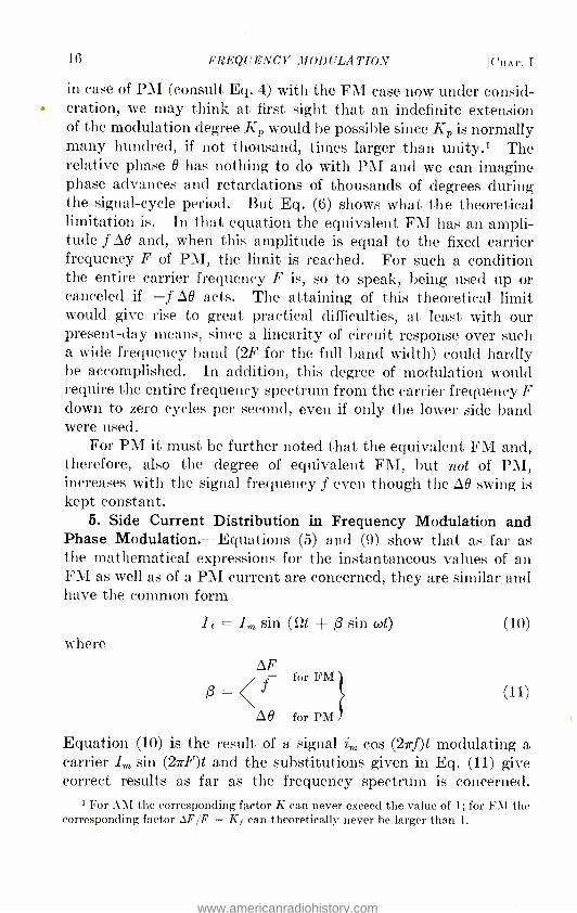
5. Side Current Distribution in Frequency Modulation and Phase Modulation. -Equations (5) and (9) show that as far as the mathematical expressions for the instantaneous values of an FM as well as of a PM current are concerned, they are similar and have the common form
where It = Im sin (12t -F- ß sin wt) (10)
OF for FM
(11)
AO for PM
ß =
Equation (10) is the result of a signal im cos (2irf)t modulating a carrier Im sin (27rF)t and the substitutions given in Eq. (11) give correct results as far as the frequency spectrum is concerned.
i For AM the corresponding factor K can never exceed the value of 1; for FM the corresponding factor AF /F = K1 can theoretically never be larger than 1.
www.americanradiohistory.com

SEC. 5] FUNDAMENTAL RELATIONS 17
Whether the time function of the ß term in Eq. (10) has a minus value, or whether it is a sinusoidal or a cosinoidal function, is a matter of how the particular modulation is produced. This is discussed on page 66.
The solution of Eq. (10) is possible by means of Bessel functions of the first kind (for mathematical details consult the Appendix). Since Eq. (11) for the modulation index ß holds for numerical values of M in radians (which is numerical), and also for the ratio AF /f, we have the same solution, as far as mathematical expres- sions are concerned, whether we deal with FM or with PM. For a maximum frequency swing OF = ±75 kc and a signal frequency f = 15 kc, we have a ß value of 5; for a maximum phase swing of M = ± 286.5 deg' we also have ß = 5. The solution of
Eq. (10) leads to the spectrum distribution
Ie = Int{Jo(ß) sin 12t + J1(ß)[sin (52 + w)t - sin (52 - w)t] + J2(ß)[sin (52 + 2w)t + sin (52 - 2w)t] + J3(0)[sin (52 + 3w)t - sin (52 - 3w)t] + J4(0)[sin (52 + 4w)t + sin (52 - 4w)t]
+ J(ß)[sin (52 + nw)t + (-1)" sin (52 - nw)t]} (12)
if OF, as well as the highest signal frequency f, is small compared with the center or mean frequency F. This is satisfied in com- mercial practice since F is in the megacycle range (for instance, 45 Mc) ; AF is at most ± 75 kc, and the largest f is at most 16 kc. That the application of this formula is simple will be seen from the numerical examples that follow.
This solution is very important as far as circuit design is con- cerned since its numerical evaluation gives the required band width that the circuits must handle. It shows, for instance, that theo- retically an infinite number of side currents of frequencies F ± f, F ± 2f, F ± 3f, F ± 4f, etc., besides a current of carrier frequency F, are possible. Since a spectrum current, whether of center or carrier frequency F or any upper or lower side current, can play only a practical part when its amplitude is relatively significant with respect to the unmodulated carrier level I,,,, the first step is to find the respective amplitudes of the carrier and the side currents.
1 One radian is 57.3 deg since 6.28 radians are 360 deg.
www.americanradiohistory.com

18 FREQUENCY MODULATION [CHAP. I
The amplitude of the carrier frequency F is ImJo(ß). The value of ß is found from Eq. (11), as already shown in the previous numerical case, where ß = 5. For the FM case where the maxi- mum frequency excursion OF is ± 75 kc and the modulating or signal frequency f is 15 kc, the carrier amplitude is I,nJ0(5) _ -0.1776In,. This amplitude is only 17.76 per cent of the unmodu- lated carrier amplitude I. Hence, for an unmodulated carrier level of 100 amp, the spectrum distribution will show at the center frequency F an amplitude of 17.76 amp. We shall find further that, for both FM and PM, symmetrical frequency distribution around the carrier or center frequency F occurs. This means, for instance, that the amplitude of the upper side current of frequency F + 3f has exactly the same value as the amplitude of the cor- responding lower side current of frequency F - 3f. For the previous numerical example, the amplitude of these side currents has the value I,nJ3(5). Since J3(5) has a numerical value of 0.3648, the amplitude, which is 3f = 3 X 15 = 45 kc below or above the carrier frequency F, is only 36.5 per cent of the unmodu- lated carrier level I,n.
We note already two essential differences between AM and FM from this numerical case. One is that many side currents are possible in FM. The other is that the frequency spectrum dis- tribution of the modulation energy in FM is such that the energy is not entirely in the first pair of symmetrical side currents as it is with AM. In general, it is spread over several side currents including the carrier current of frequency F. A third difference is that for AM the equal amplitudes for the only possible side - current pair of respective frequencies F -f and F + f can never become larger than 0.51m, since for 100 per cent amplitude modula- tion K = 1 and the side- current amplitudes are, according to Fig. 5, equal to 0.5KIm.
Moreover, from this numerical example, we note that for FM the spectrum equation (12) shows that for ß = 5 the center - frequency amplitude is only 17.76 amp. Yet the symmetrical amplitudes of the third side- current pair, 45 kc below and 45 kc above the center frequency F, are as 'much as 36.5 amp; i.e., these amplitudes are larger than the carrier -frequency component.
Since the side -current distribution equation (12) holds for both FM and PM, exactly the same numerical results for the respective amplitudes in the spectrum would hold for PM with a maximum
www.americanradiohistory.com

SEC. 6] FUNI)AMEN7'AL RELATIONS 19
phase swing of 57.3 X 5 = 286.5 deg. Hence, equal values of
the modulation index ß, whether due to PM or to FM, yield the same spectrum distribution. In spite of this fact there is a great difference between FM and PM, since it is not only the value of ß that counts but also the cause that produces this value. This can be readily understood from Eq. (11). For PM, the value of the modulation index is equal to the maximum phase deviation M. Hence, for a fixed maximum phase swing it does not matter whether a 50 -cycle signal or a 15 -kc signal modulates the phase of the carrier current. In either case we shall havé the same num- ber of important side- current pairs with the corresponding ampli- tudes. However, for instance, for the tenth upper and lower side current in the 50 cycles per second signal frequency case, the same amplitude pair is 10 X 50 = 500 cycles per second above or below the carrier frequency F; for the 15 -kc signal it is 150 kc above and below the carrier frequency F. Hence, the latter case refers to a much wider pass -band width. This is discussed further in Sec. 7.
In the case of FM matters are different, since the modulation index ß is directly proportional to the maximum frequency swing OF, which causes the FM, and indirectly proportional to the signal frequency f. For AF fixed at a value of ± 75 kc, we find for a 15 -kc signal frequency an index ß = 5. This causes in Eq. (12) approximately eight important side currents on each side of the carrier or center frequency F, and, therefore, a band width of 8 X 15 = 120 kc on each side of the carrier frequency. But for a 50 -cycle hum modulation, the value of the index becomes very large if the same AF value (as used in commercial practice for the upper limit) is preserved and ß is equal to 1,500. As will be shown, we have then an almost continuous spectrum distribution with essentially 1,500 side currents on each side of the carrier frequency and, therefore, a total band width of essentially 2 AF = 150 kc. Hence, in the case of FM, the number of important side currents is larger for the lower frequencies in the signal band than it is for the higher pitch signals, even though AF is kept constant for all signal frequencies f.
6. Application of Bessel Tables and Bessel Curves. -Since to evaluate Eq. (12) it is necessary to obtain the values of the various Bessel factors, J0(0) for the amplitude of carrier frequency F, J,(ß) for the amplitudes of frequencies F -f and F + f, J2(ß)
www.americanradiohistory.com

20 FREQUENCY MODULATION [CHAP. I
for the side- current pair of frequencies F -2f and F -}- 2f, J3(ß) for the next side- current pair of frequencies F -3f and F 3f, etc., some useful tables and curves are given here as well as in the Appendix. The curves, although not accurate enough for many calculations, have the advantage of showing directly the variation of the amplitude values for FM and PM. The tables give more accurate results and a means for plotting certain curves so that graphical interpolation is possible. In the Appendix are formulas from which Bessel factors can be computed.
TABLE I*
O Jo(R) Ji(R) J2(0) J3(I1) J4(13)
0 1.0000 0 0 0 0
0.1 0.9975 0.0499 0.00124
0.2 0.99 0.0995 0.00498 0.00017 0.0000042
0.3 0.9776 0.1483 0.01117
0.4 0.9604 0.1960 0.0197 0.0013 0.000067
0.5 0.9385 0.2423 0.0306
0.6 0.912 0.2867 0.0437 0.0044 0.000331
0.7 0.8812 0.329 0.0589
0.8 0.8463 0.3688 0.0758 0.0102 0.001009 0.9 0.8075 0.4059 0.0946
1.0 0.7652 0.4401 0.1149 0.0196 0.002477 1.2 0.6711 0.4983 0.1593 0.0329 0.005023 1.4 0.5669 0.5419 0.2073 0.0505 0.009064 1.6 0.4554 0.5699 0.257 0.0725 0.014995
2.0 0.2239 0.5767 0.3528 0.1289 0.03399
2.4 0.0025 0.5202 0.4311 0.1981 0.064307 2.8 --0.2601 0.3391 0.4783 0.2728 0.10667
*J0(ß), J1(ß), J3(4), and J4(ß) are the factors by means of which the carrier level T. has to be multiplied.
Table I gives the successive amplitude factors by which the unmodulated carrier level Im is to be multiplied in order to obtain the magnitude of any particular current in the frequency spectrum. It is just as easy to read the values from such tables and to apply them as it is to use trigonometric tables. For instance, for a maximum frequency swing of AF = ±20 kc and a 10 -kc signal frequency, we find that ß = OF /f = 20ío = 2. Table I discloses that J0(ß) = 0.2239 is the value of the factor by which Im has to he multiplied in order to obtain the magnitude of the component
www.americanradiohistory.com

SEC. 61 FUNDAMENTAL RELATIONS 21
of the center frequency F. The value of J1(0) = J1(2) = 0.5767 when multiplied by I,,, gives the amplitude of either the first upper side current of frequency F 10 kc or the amplitude of the first lower side current of frequency F - 10 kc. It does not matter what the value of the carrier or center frequency F is, as long as
0.6
0.5
0.4
0.3
0.2
+Jn(2) 0.1
0
-Jn(2)-0.1
-0.2
-0.3
0.4
-0.5
-0.6
J,(2)
L
JZ(2)- J (2)
Jo(2)
J4(2) I -30 -10 J4(2)
-40kc 1 -20 F +10
polarity
+20 +30 +40
side current factor with
to magnitude (eq. /2)
kc
-J3(2)
[1w1/th
Significant amplitude respect and
-J,(2)
0.6
0.4 a)
--a 0.3
's 0.2 -6
0.1
0
For actualI multip /y t ordinate ,
unmade" level I,,,
Carrier carrier I be sm F- -0.5 W - - -- - -- Al /a
s, Ff -40 -30 -20 -10 F +10
Fn;. 8.- Spectrum distribution for a modulation index of 0 = 2.
it is large enough to accommodate the FM. The succeeding value: in the ß = 2 line of Table I, then, are the factors that give the relative intensities of the successive side currents more remote from the carrier frequency F. Inasmuch as all amplitudes are obtainei by multiplying these Bessel factors by the same value, namely I,,,, the magnitudes of the factors determine directly the relative
+20
mphlude, e respective
ength by the fated carrier . (Note that the amplitude can a / /er than unity; mp /nude factors drawn for
ame polarity)
+30 +40 kc
www.americanradiohistory.com

22 FREQUENCY MODULATION [CHAP. I
intensities of the side- current pairs in the useful frequency spec- trum. It is, therefore, correct if we plot only the Bessel values as shown in Fig. 8. Any other amplitudes farther away from the carrier frequency F than those shown have only a theoretical significance. The total band width is, therefore, 80 kc; i.e., it is much wider than the peak -to -peak frequency swing 2 OF = 2 X 20 = 40 kc. It should be clearly understood that it is the number of important side currents and their corresponding frequencies that count in determining the required band width. It is not necessarily the peak -to -peak frequency swing 2 AF that causes the FM.
It must be admitted that without the preceding theoretical speculations it would hardly be possible to approach or to guess such design formulas as are presented in this publication. The assumption of such a relatively small frequency deviation as ±20 kc, as used in the foregoing numerical example, is by no means out of place as far as practical applications are concerned. The ±75 kc standard set by the FCC refers only to the maximum permissible swing above or below the carrier frequency F. The ±20 -kc case in the example refers simply to a less intense FM; i.e., it refers to a sound probably weaker than the average loudness.
Bessel curves, as shown in Fig. 9, lead to even quicker specula- tions and are just as easy to apply as is the table of values. The J0(ß) curve gives again the respective amplitude factors for the modulated component of the carrier frequency F for various values of the index ß. It has already been mentioned that, unlike AM, we have in FM as well as PM a spectrum distribution of the modulation energy (proportional to the square of the spectrum amplitudes), which also affects the amplitude of carrier frequency F. Figure 9 shows this fact plainly. For the case when no FM exists there can be, no frequency swing, i.e., OF = 0 and, therefore, ß = 0. For ß = 0, there exists only one Bessel factor, namely, J0(0) = 1. The amplitude factor for the first side -band pair starts out with zero value and, therefore, no first side -band pair is possible. All other Bessel curves, such as J2(ß) and J3(ß), also start with zero values for zero values of ß (shown in other curves but not in Fig. 9).
The J0(3) curve, as well as all other Bessel curves, resembles damped wave trains; i.e., they intersect the zero or ß axis. These points of intersection are of importance. For instance, this happens for ß = 2.4048, 5.5201, 8.6537, 11.7915, 14.931, 18.071,
www.americanradiohistory.com

SEC. 6J FUNDAMENTAL RELATIONS 23
21.212, 24.353, 27.494, 30.635, etc., for the MO) curve determining the amplitude for the carrier frequency F. Hence, if the ratio of maximum frequency swing OF to the signal frequency f assumes such values as already given for ß, the carrier amplitude must disappear altogether.
This leads to an experimental method for determining the maximum frequency deviation OF since the ß values for which the carrier amplitude vanishes is known from the above values.
+1.0
+0.9
+0.8
+0.1
+0.6
m+0.5 4+04 -45
Fs +0.3
m+0.2
-7 +0.1
Jo 651-Mu/Ober for amp/dude [Jo (,B)J /,,, of center frequency F
J, 031 -Mu/tip/ier for amp/i/udes[J, 03lPm of side frequencies Fi f
1- . : Jo Gel
MI lit ,
11 1 0 ' t\t'/i sir!,
3 Jill
4 5 6 7 8 9 10 II 12 13 14 15 16 17 18 19 20 Modulation index ß
Flu. 9.- Bessel curves by means of which the magnitude or the amplitude of center fre- quency F and of respective side frequencies F ± f can he computed.
The signal frequency f is also known. The two curves of Fig. 9 show also that with increasing values of ß the modulated carrier amplitude decreases at first toward zero. Then it becomes negative and more negative, decreases again its negative value, and becomes zero again for ß = 5.5201. Then it builds up again to increasing positive amplitudes, etc. At the same time the amplitude of the first side- current pair also undergoes changes determined by the J1(ß) curve. Table II gives the amplitude factors for ß values up to 12 and for a spectrum distribution up to the fifteenth side- current pair, since J15(ß) stands for the multiplier of the unmodulated carrier level I,,, for the side currents of fre- quencies F - 15f and F 15f. For instance, the multiplier
www.americanradiohistory.com

24 FREQUENCY MODULATION [CHAP. I
for the eleventh side -current pair for a modulation index of = 3 is J11(ß) = J11(3) = 0.00000179. Hence, this is a side -
current pair that cannot play a practical part. Table II is very useful. In places where no values are given, the values are zero, or practically so.
TABLE II.- BESSEL FACTORS UP TO THE FIFTEENTH SIDE CURRENT PAIR AND FOR A
MODULATION INDEX (3 UP TO 12
(3 J0(ß) J1(ß) J2(0) J3(0) J4(ß) J5(43) J6(ß) J7(0)
1 0.7652 0.4401 0.1149 0.0196 0.0025 0.00025 0.0'21 0.0515
2 0.2239 0.5767 0.3528 0.1289 0.034 0.00704 0.0012 0.0'175
3 -0.2601 0.3391 0.4861 0.3091 0.1320 0.04303 0.0114 0.02255
4 -0.3971-0.066 0.3641 0.4302 0.2811 0.1321 0.0491 0.0152
5 -0.1776-0.3276 0.0466 0.3648 0.3912 0.2611 0.131 0.0534
6 0.1506-0.2767-0.2429 0.1148 0.3576 0.3621 0.2458 0.1296
7 0.3001-0.0047-0.3014-0.1676 0.1578 0.3479 0.3392 0.2336
8 0.1717 0.2346 --0.133 -0.2911 -0.1054 0.1858 0.3376 0.3206 9 -- 0.0903 0.2453 0.1448-0.1809-0.2655-0.05504 0.2043 0.3275
10 -0.2459 0.0435 0.2546 0.0584 -0.2196 -0.2341 1- 0.0145 0.2167
11 --0.1712--0.1768 0.139 0.2273 --0.015 -0.2383 --0.2016 0.0184
12 0.0477 --0.2234 -0.085 0.1951 0.1825 -0.0735 0.244 --0.1703
ß J8(ß) J,(ß) J10(0) J11(13) J12(13) J13(0) J14(0) J15(13)
1 0.0794 0.08525 0.002631 0.01012 0.0125
2 0.04222 0.0525 0.0625 0.0'23 0.0 819
3 0.03493 0.04844 0.041293 0.05179 0.06228
4 0.02403 0.0'94 0.0'195 0.0'37 0.05624
5 0.01841 0.02552 0.021468 0.0'351 0.04763
6 0.05653 0.0212 0.02696 0.02205 0.03545
7 0.128 0.0589 0.02354 0.02833 0.02266
8 0.2235 0.1263 0.0608 0.0256 0.0096 0.0033
9 0.3051 0.2149 0.1247 0.0622 0.0274 0.0108 0.0039
10 0.3179 0.2919 10.2075 0.1231 10.0634 10.0297 10.012 10.00451
11 0.225 0.3089 0.2804 0.201 0.1216 0.0643 0.0304 0.013
12 0.0451 0.2304 0.3005 0.2704 0.1953 0.1201 0.065 0.032
These factors multiplied by la yield the various spectrum amplitudes.
Figure 10 shows a very convenient form of presenting Bessel functions for use in estimating the required band width for circuit design. The curves are drawn for a constant modulation index ß; the ordinate intersections with the respective curves give directly
www.americanradiohistory.com

SEC. 61 FUNDAMENTAL RELATIONS 25
the multiplier J,,(ß), where n stands for the order of side- current pair. For n = 0, we have only one current, of carrier frequency F. When, for instance, the J6(ß) ordinate, i.e., the multiplier for the amplitudes of frequencies F -6f and F -+ 6f, is of interest, it will
be seen directly, without resorting to the more accurate Table II or to tables in the Appendix, that for ratios of SF /f, as well as
maximum phase swings of AO, smaller than about 3, the number of
Maximum frequency deviation OF
F/ Signal frequency f +0'8 A4- Maximum phase deviation dB in radians
+01
iikt.
,..../3-1 Only values ofn =OJ ZJ,4,etc.play
6 B'2 a practical part
+0.5 ,B =/ Jn /B)JIm is amplitude ' _6 ofparticularspectrum
+ current if Im denotes 0 4'.1,,,',r ÍB=9 the carrier level for
L +a3 !ili 'w a iia /'- no modulation
+o.z 1'1 Lie`:11:1 /:elk %% MIIIIMM WM/M. 111\IATIM P1311M`W` 1 IA1MMII/Ii I,V INI1 \III/ IITAUTAIMMA
-02 íI11%1 AEI/ -0.31IFMr WPM -0.4'mV J3(ß)4 function
/B)J (ß)
-0.5
co_ co_ o
- -0.1
j7669
6
10034,68)
(6IJ9 /B)Jio /B) i /Ql
68)Jsif)J6r6) Order fo Bessel
(fi)
-06 Fu >. 10.- Curves for fixed modulation index ß with respect to the order n in the function
J.(1.1). (By means of these curves the band width can be read off directly.)
significant side currents can never exceed six side -current pairs.
A value of ß = 3 causes practically a band -pass width of 2 X 6f,
since six upper and six lower side currents play a practical part. A value of ß = 2 requires only a band width of 2 X 5f, where f is the frequency of the signal current, i.e., the current that modu- lates the carrier. Further details will be given in Sec. 7.
Figure 11 gives a practical example of how the Bessel factors are used. This example is for a case where the modulation index ß
is 10. From our theory we know now that it does not matter whether we deal with the deviation ratio SF /f = 10 in case of FM, or with a maximum phase deviation AO = 10 radians or 573 deg
in case of PM. This is strictly true as far as the number of
important side currents that play a part and as far as the respective
www.americanradiohistory.com

26 FREQUENCY MODULATION [CHAP. I
relative amplitudes of these side currents are concerned. But it should be understood that for PM the spectrum distribution of Fig. 11 holds for all signal frequencies as long as the maximum phase swing M that causes the PM is kept fixed. It is to be under-
1
5141 . S/3
5.12 +F)If
'
1 S I
SnF+ 10f ¡ 1
I, 1/0 1 I 1 F+9f I I I
`S91 1 1 1 i; F+Bf ¡ i H 1 1 FY- ¡ +
1 1
SB I 187
' 1 1
S8
F4-3f I I
521 I F+2f ¡
i
031-1- ,1
S/ IF^f
I
' F-2f S2
i 1 1 1
.á --- 4,
a _-_- Q L.L.
á T ti \ j LI.>
u Li
t. --1
-`6 I ; , F+Sf I
i 1 S 1
I ' i F-1-4f1
i 1 1 5 1
°'
i ; I l i i I
1 1S4 1
JR
;CcrrrieroffrequencyF 1
1 f Si i i i i i i
11 I
SZF1T I I
S14'
, I
I I ¡ I I
1 I 1 I I
I I I I I 1 I I I I I I
I I I I
I I
I
I 1 , I , , , , , , , , I
0.3 02 0.1 0 -0.1 -02 -03 Amplitude Jr) (ß)-"E--- for n =0 for the carrier of frequency F
n= I for the first side current pair F ±f n= 2 for the second side current pair F± 2f n =3 for the third side current pair F ±3f
n=14 for the SI4 pair of frequencies F -14f and F +14f FIG. 11.- Amplitudes of significant currents in the frequency spectrum for ß = 10. (Note
above distribution holds for both FM and PM.)
stood, however, that for a 50 cycles per second signal current the frequency spacings between consecutive spectrum currents is 50 cycles per second wide, just as for a 15 -kc modulating current this spacing becomes 15 kc wide. For FM, however, the dis- tribution of Fig. 11 holds for the entire signal- frequency range only if the maximum frequency deviation OF that causes the FM
www.americanradiohistory.com

SEC. 6] FUNDAMENTAL RELATIONS 27
changes directly with the signal frequency f, otherwise the deviation ratio SF /f cannot remain equal to 10. Hence, the maximum frequency deviation AF indicated in Fig. 11 is correct only for a definite value of the signal frequency f. For instance, for a 15 -kc modulation frequency, AF would have to have a value of 150 kc in order to render ß = 10, while for a 1,000 -cycle note AF would have to be only 10 kc.
As far as the method of construction of the frequency dis- tribution of Fig. 11 is concerned, use Table II and look at the various values on the ß = 10 line. This line is especially marked in Table II for the sake of this numerical example. These values in succession are: - 0.2459 for the carrier frequency F is the multi- plier for Im; 0.0435 for frequencies F -f and F f; 0.2546 for the next side- current pair of frequencies F -2f and F 2f ; etc. Table II shows that it is of no use to go much farther than to 14 side currents on each side of the carrier frequency since the amplitudes of additional side currents will be negligibly small. Hence, the band width for the modulation index ß = 10 is 2 X 14f. This means that for a 15 -kc signal the band width would be 28 X 15 = 420 kc; for a 1,000 -cycle note it would be only 28 kc. We see already that the highest modulating frequency requires more fre- quency space as far as circuit design is concerned. For this reason a maximum deviation ratio OF /(highest signal f) is chosen equal to 5 in modern transmitter design. Assuming 15 kc as the highest signal frequency, this value of 5 will give a maximum frequency swing equal to 5 X 15 = 75 kc. Hence, for the most severe band- width condition of ,3 = 75/15 = 5, we find from the ß = 5 curve in Fig. 10 that the curve creeps into the zero reference axis between the J8(ß) and the J9(ß) ordinates, but closer to the J8(ß) ordinate. It does not matter how close it is since, according to Eq. (12), the ninth side -current pair must follow the eighth side- current pair as fractional side -current frequencies do not exist. The ß = 5
curve in Fig. 10 shows only a small value for the eighth side - current pair and a value of practically zero for the ninth side - current pair. Hence, we have only eight side currents on each side of the carrier frequency F; therefore, we have a band width of 2 X 8 X f = 16 X 15 = 240 kc.
The transfer networks have to be designed for this frequency band width, whether they are located in the transmitter or in the receiver. Hence, the i-f stages in a receiver have to pass such a
www.americanradiohistory.com

28 FREQUENCY MODULATION [CHAT. I
frequency band. This is also required for the input network of the discriminator (for details, page 78), but not for the discrimina- tor or slope characteristic of the demodulator or FM detector. The reason for this is that the slope characteristic of the demodula- tor translates FM into AM and, hence, depends like the FM transmitter, i.e., the modulator unit of the transmitter, only on the maximum value of the frequency deviation F. Hence, theoretically, we require a slope characteristic that can handle the peak -to -peak frequency swing for the condition of maximum deviation, which is 2 X 75 = 150 kc. Since the degree of linearity of a slope detector decreases at the upper and lower ends of the slope characteristic, it seems best to design the slope for somewhat more than 150 -kc linearity.
That the maximum deviation ratio 75/15 takes care of the most severe condition, as far as the band width and the entire f range are concerned, can also be seen from the following analysis. Suppose we assume a 5 -kc signal, then the value of ß = 7% = 15. From the Bessel factors given in the Appendix, we find that at most 20 side currents on each side of the carrier can play a part. Hence, a frequency space of only 2 X 20 X 5 = 200 kc is required. For the lower signal -frequency range, very large ß values are obtained, resulting in, as a matter of fact, almost a continuous spectrum. For these low signal frequencies the band width becomes essentially equal to the peak -to -peak frequency swing, which is 150 kc.
7. Numerical Speculations on Frequency Swing, Equivalent Phase Swing, and Band Width. An account has just been given of why a maximum frequency swing of ±75 kc was chosen. Besides, the good feature exists that such a large swing can override unde- sirable phase flutter and its equivalent frequency flutter.
It is now of interest to learn how the peak -to -peak FM swing, i.e., the value of 2 OF, is related to the actual significant frequency distribution. We shall again do this for PM and FM. Figure 12 illustrates the case for PM and Fig. 13 the case for FM. For both figures the same amplitude scale was used throughout, as well as the same frequency scale. This permits, then, a direct comparison of the two. In Fig. 12 three cases are compared, but all cases are for one and the same maximum phase deviation of 5
radians or 5 X 57.3 = 286.5 deg. Only the significant side - current amplitudes are shown, which were obtained as described
www.americanradiohistory.com
SEC. 7] FUNDAMENTAL RELATIONS 29
in Sec. 6. We note that for a 10 -kc modulating frequency, the spectrum width required comes out as 160 kc ; for a 5 -kc signal this width is reduced to 80 kc; for a 1,000 -cycle note the required width is only 16 kc.
Since with PM the modulation index ß is equal to the value of
the maximum phase swing M which causes the PM, the correspond- ing side -current amplitudes for the upper, middle, and lower dis- tributions shown in Fig. 12 are all alike. They have exactly the same magnitude regardless of the value of the signal frequency f. Hence, for PM and for fixed M swing, we have just as many side currents for the higher tones as for the lower tones. However, the highest desired signal frequency requires the widest band width, just as was already found for the case of FM. Since we preserve the same number of side currents as well as the same relative mag- nitudes, all that happens is that for the lower signal frequencies the energy spectrum is more crowded together. This means that a band -pass network can be used more efficiently. By efficient use of a band -pass network is meant that the frequency space is
more filled up with amplitudes that convey the signal. As far as the band -pass network design is concerned, this concentration of energy in a narrow band does not play a part. It is the width of the pass band, not the energy in a given width, that affects the problem of designing a filter.
With respect to Fig. 13, a constant frequency swing OF equal to 50 kc was assumed. In order to permit a clear representation, only cases down to a signal frequency f = 2.5 kc are illustrated in Fig. 13. Otherwise too many side currents would have appeared. Since for FM the signal frequency affects the value of the modula- tion index ß, if OF that causes the FM is fixed, we have more side currents for the lower tones than for the higher ones. The filling up of the frequency space is due not so much to crowding the spectrum together as to an increase in the number of significant side currents as the signal frequency is lowered. As a matter of fact, the so- called " crowding together" of the frequency spectrum is
limited. The limit is reached when the total band width due to significant side currents becomes equal to the peak -to -peak fre- quency swing, i.e., equal to 2 F. This occurs for large OF swings in the lower signal- frequency range. The higher the signal frequency, the more the actual band width required exceeds the peak -to -peak swing that causes it.
www.americanradiohistory.com

30 FREQUENCY MODULATION [CHAP. I
It is now of interest to learn what happens when small ß values occur. The representations to the right of Fig. 14 show what we may expect. These Bessel factors for the multiplier of the normal carrier level Im used to obtain the amplitude of the carrier fre-
r
F-6f
F 8f I
F- 7f
Sand width w = /60kc for f = /0kc F-4f F1-4f
F- f Fi-3f
8=a8 =5radians
F -2f F4-2f I I
Carrier._
F-Sf
F-3f
,B=4B= 5radians
F-8f I
I
F
F+f
=Z0=5 radians
E
F+S f
80 k
I II, F+8f
w=80kc j for f=5kc
F+6f I F+7fFt8f I I
J These three representations are all for the same phase deviation 48 and show how the respective amp/if/des preserve their intensify but spread More as the signa/ frequency fis raised. The LONESTsigna /frequency f requires the SMALL EST PASS BAND
- w= 16 k forsigna/ frequency f= 1 M
FIG. 12.- Current distribution for phase modulation of fixed maximum phase swing. AB = 5 radians.
quency F, the amplitude of the first side -current pair of frequencies F -f and F + f, the amplitude of the second side -current pair of frequencies F -2f and F + 2f, and the amplitude of the third side -current pair of frequencies F -3f and F + 3f are again drawn to exactly the same amplitude scale. The ß scale is also the same so that a direct comparison of the curves is possible.
www.americanradiohistory.com

SEC. 7] FUNDAMENTAL RELATIONS 31
It will be noted that the multiplier for the modulated carrier amplitude of frequency F, which is J0(ß), starts out with unity value; i.e., its value is unity for ß = O for which value of ß neither FM nor PM can exist. The multiplier for the first pair of side - current amplitudes, which is J1(ß), starts out with zero value.
Band width /60kc fora signal frequency f =10kc
F-8f I
Cif' S0_ fi -f =%0-5
I I I
Carrier% 80kc1 - dF =f50kc F +8f
F Note that for the upper spectrum distribution the half band width considerably exceeds aP
Band width /40 kc for f =5kc
r F- 24f
I
F+14f
Band width 120 k for f =2.5 kc SO _ aF=t50kc fi 25-20
'
I hF+24f 1,
I F
I
FIG. 13.- Amplitude distr'bution of the component currents in frequency modulation for different modulation index 43 = OF /f.
The reason for this is that J1(0) _ - d[J0(0)] /dß. Hence, for a portion of the J0(ß) curve where the curve progresses horizontally, the rate of change with respect to ß must be zero. Moreover, it is seen that for the second side- current pair the multiplier J2(ß) slides into the ß axis, for practical purposes at least, for values of ß somewhat larger than zero. This is still more the case for the multiplier J3(ß).
www.americanradiohistory.com

32 FREQUENCY MODULATION [CHAP. I
The representation to the left of Fig. 14 shows that the higher the order of the side -current pair, the larger the value of ß has to be before the multiplier causes an appreciable amplitude of the particular side currents of that order. For instance, the ampli- tudes for the eighth side- current pair corresponding to frequencies F - 8f and F + 8f can play a practical part only when the modula- tion index ß is larger than 3. Hence, any other still higher orders of side currents, such as F ± 9f, F ± 10f, or F ± 11f, will have still less noticeable amplitudes for ß values smaller than 3. The J16(ß) curve indicates that side currents of frequencies F - 16f and
0.5
0.4
0.3
;,-; 0.2
0.i
0
E -0.2
0.3
0 15 20 i l
0 2 4 AF
--ß -f Le radians
FIG. 14.- Relative spectrum current amplitudes change with the value of the modulation index /3.
2(B) ,, (!g) -8 (ß) New is6)
11"I n-3 //\ I1NI11/1 Mik //I11111WIII1\!=\\ II11\ I 1'\\\'11l 11\1: IÌ AÌM Ï1:,PV I Ï\ \\ ÏÌ IÏ I\1\\ÏÌÌ\\\%\ lÏ ®11\IIIIiU\MF/\Ifa,1i :1\'Il1\Vi\J\J\ 111.III n 8
I I
n =/6
LO 0.8-
Jo(ß)Ó4- 0.2 - o
0.6- J,(ß) óz-
0
0.6- l
JZ(ß>oz II
P=0.2
Carrier F
o F±2f
0.6-
J3(ß) 02- I F+3f
5 10 F
pa6 radians
F -{- 16f and the following side currents of respective frequencies F ± 17f, F ± 18f, F ± 19f, etc., for ß values smaller than about 11, for all practical purposes do not exist. Hence, in the case of FM, such curves as those shown in Fig. 14 and curves shown at other places in this publication or plotted from tables, give a ready means of determining at sight how many side currents have to be taken into account; i.e., what band width the various circuits must be designed to handle.
It should be borne in mind again that with FM the maximum frequency deviation OF that causes the FM by no means always predicts the correct band width. However, the maximum devia- tion ratio AF/f, for a fixed upper AF limit will do this, since it causes the largest frequency spectrum spread. On the other hand, with PM the maximum phase deviation limit M gives
www.americanradiohistory.com

SEC. 7] FUNDAMENTAL RELATIONS 33
TABLE 111.- ESTIMATING BAND WIDTH
OF
f radians*
Carrier frequency and successive significant side currents expressed in percentage of the
unmodulated carrier level I,,,t
Required band width
Maximum equivalent phase shift,
degrees
M = 57.3 f 0.01 100; 0.5 2f 0.573
0.02 99.99; 1 2f 1.146
0.03 99.98; 1.5 2f 1.719
0.04 99.96; 2 2f 2.292
0.05 99.94; 2.5 2f 2.87
0.1 99.75; 4.99 2f 5.73
0.2 99.00; 9.95 2f 11.46
0.3 97.76; 14.83 2f 17.19
0.4 96.04; 19.6 2f 22.92
0.5 93.85; 24.23; 3.1 4f 28.7
1.0 76.52; 44.01; 11.49; 1.96 6f 57.3
2.0 22.39; 57.67; 35.28; 12.89; 3.4 8f 114.6
3.0 26.01; 33.91; 48.61; 30.91; 13.2; 4.3; 1.14 12f 171.9
4.0 39.71; 6.6; 36.41; 43.02; 28.11; 13.21; 4.91; 1.52 14f 229.2
5.0 17.76; 32.76; 4.66; 36.48; 39.12; 26.11; 13.1; 5.34; 16f 287
1.84 6.0 15.06; 27.67; 24.29; 11.48; 35.76; 36.21; 24.58; 18f 343.8
12.96; 5.653; 2.12 7.0 30.01;0.5;30.14 ;16.76;15.78;34.79;33.92;23.36; 22f 401.1
12.80; 5.9; 2.3; 0.8 8.0 17.17; 23.46; 11.3; 29.11; 10.54; 18.58; 33.76; 24f 485.4
32.06; 22.35; 12.63; 6.1; 2.6; 0.96 9.0 9.03; 24.53; 14.48; 18.1; 26.55; 5.5; 20.43; 32.75; 26f 515.7
30.51; 21.49; 12.47; 6.2; 2.73; 1.1
10 24.59; 4.35; 25.46; 5.83; 21.96; 23.41; 1.45; 21.67; 28f 573
31.79; 29.19; 20.75; 12.31; 6.34; 2.9; 1.2
12 4.8; 22.34; 8.5; 19.51; 18.25; 7.3; 24.37; 17.03; 4.5; 32f 687.6
23.04; 30.05; 27.04; 19.53; 12.01; 6.5; 3.2; 1.4
15 1.4; 20.51; 4.2; 19.40; 11.92; 13.05; 20.61; 3.45; 38f 859.5
17.40; 22; 9; 9.99; 23.67; 27.87; 24.64; 18.13; 11.62; 6.6; 3.5; 1.66
18 1.34; 18.8; 0.75; 18.63; 6.96; 15.54; 15.6; 5.1; 46f 1031.4
19.59; 12.28; 7.3; 20.41; 17.62; 3.1; 13.16; 23.56; 26.11; 22.86; 17.06; 11.27; 6.7; 3.7; 1.9; 0.9
21 3.7; 17.11; 2.02; 17.50; 2.97; 16.37; 10.76; 10.22; 52f 1203.3
17.57; 3.2; 14.85; 17.32; 3.3; 13.56; 20.08; 13.21; 1.2; 15.05; 23.16; 24.65; 21.45; 16.21; 10.97; 6.77; 3.86; 2.05; 1
24 5.6; 15.4; 4.34; 16.13; 0.3; 16.23; 6.4; 13; 14.04; 58f 1375.5 3.6; 16.77; 10.33; 7.3; 17.63; 11.8; 3.9; 16.63; 18.31; 9.3; 4.3; 16.19; 22.64; 23.43; 20.31; 15.5; 10.7; 6.8; 3.99; 2.2; 1.1
* Holds also for t First number 3enotes the percentage amplitude of carrier frequency F; second number is the per-
centage amplitude tor side frequenciesF -f and f; the third number holds for frequenciesF 2f; etc.
www.americanradiohistory.com

34 FREQUENCY MODULATION [CHAP. I
directly a means for estimating the correct band width. This limiting phase excursion is directly the value of ß and does not change with the variation of the signal frequency f. Table III shows what occurs when the ß value is changed over wide ranges. All amplitude values are given as positive quantities, since the purpose of this table is only to determine the required band width for a particular AF /f ratio. The polarity of the various Bessel factors is, therefore, of no concern. The significant amplitudes shown are so chosen that the side currents for which the amplitudes are less than 1 per cent of the unmodulated carrier level Im are neglected. This is quite conservative from an engineering point of view.
-Maximum ß =24
.111 I I I I I hi. F-30f F FII+30f
[4 Band widfh w = 60f FIG. 15. -All significant spectrum amplitudes are drawn with the same polarity in
order to show how the spectrum energy due to modulation is spread towards each side of the carrier of frequency F.
Examination of Bessel tables will show that the greater the value of the modulation index ß, whether due to AF /f or to AO
radians, the more side currents play a part. The modulation energy moves, so to speak, farther out on each side of the carrier frequency F. This gives a ready means of estimating where to stop with important side currents. For instance, for AF /f = 24, we obtain the spectrum distribution of Fig. 15. Note that the largest side -current amplitudes occur near the edges of the pass band. Hence, it is only necessary to read off, for a certain value of ß, the consecutive Bessel factors or amplitude multipliers until the very largest factor is reached. After this it is necessary only to continue reading off the following consecutive Bessel factors until, say, only 1 per cent of the unmodulated carrier level Im
is reached. Since all factors are multiplied by one and the same carrier level Im, the unmodulated carrier level in terms of the
www.americanradiohistory.com

SEC. 7] FUNDAMENTAL RELATIONS 35
Bessel values is unity. This is the largest value that can ever occur since it holds for ß = 0 and happens for Jo(0) = 1. If we are satisfied with significant terms, above 5 per cent of the unmodu- lated carrier level 'm, then we stop reading off values when the 5 per cent limit is reached.
The frequency band width in Table III is obtained by counting the number of significant side currents. For the value ß = ] 2
we note that there are, in addition to the carrier frequency term of 4.8, 16 side currents on each side of the carrier frequency F. Hence, if f is the frequency of the current that modulates in FM, the required band width is 32f. Following up the successive band widths in Table III, we note that there is a definite progression so that we can use this table for estimating any band width for values of OF, f or AO that are not given in this table but are within its range. For instance, a modulation index of 15 gives, according to this table, a frequency spread of 38f, and a modulation index of 12 gives a spread of only 32f. Hence, a value of ß = 14 must lie somewhere between these two values. Good interpolation is obtained if we plot OF /f against band width. There are only two places in this table where the progression of additional important side currents shows more than a proportional increase. One such place occurs for ß = 7. The reason for this is that for this value of modulation index ß a side current was included that had a value of only slightly less than 1 per cent. It is the extreme significant side current shown with a value of 0.8 per cent. Because such an addition of one extra Bessel factor means two extra side currents, this will increase the apparent band width by 2f. This side -current pair could have been neglected. The reason why side- current pairs below 1 per cent cannot have much effect is because the modulation power in each side current is
proportional to the square of its amplitude. Table III shows also that for small values of OF /f, we have
only one significant side- current pair, as for AM. The amplitude of the center or carrier frequency F is then essentially equal to the unmodulated carrier level, or at least practically so, for all values of ß <_ 0.2. This fact can also be seen from inspection of the Bessel curves given in Fig. 14. This leads, then, to a further simplification' of Eq. (12) since only the Jo and the Ji factors for these small values of ß play a practical part.
' See p. 37.
www.americanradiohistory.com

36 FREQUENCY MODULATION [CHAP. I
The last column of Table III gives the values of the equivalent maximum phase swing in degrees. The values in the SF /f column are also maximum phase swings in radians. Hence, this table can be used for PM also.
We have, therefore, the formula
AO = 57.3 -
deg (13)
For OF = ±75 kc, with f = 15 kc as the highest useful audio frequency to be transmitted, we find from Eq. (13) that the maximum equivalent phase deviation is AO = ± 286.5 deg. For the lowest useful audio frequency of f = 50 cycles per second, we have 0O = ±86,000 deg. This is a very large value of phase deviation if PM has to be instrumental in producing equivalent FM with large equivalent frequency swings. This difficulty can be overcome by causing PM with maximum phase swings, which are M' = M/f and which have, therefore, all the features of FM. Fortunately, we have also methods available for multi- plying the phase swings and, therefore, also the equivalent fre- quency swings. Methods are also available whereby the frequency swing can be multiplied much more than is the carrier or center frequency F itself.'
It is now an easy task to compute the degree of phase shift multiplication needed if indirect FM is used in a transmitting system. If we have to deal with indirect FM where the maximum phase excursion is never to exceed 0.5 radian or 28.65 deg, a phase swing multiplication of 86,000/28.65 = 3,000 times is
required for a signal frequency of f = 50 cycles per second and a
maximum frequency deviation of OF = ±75 kc. For the highest desired signal frequency of f = 15,000 cycles per second, a multi- plication of only 286.5/28.65 = 10 times is required. This shows why, with indirect FM designed for small distortion (about 10 per cent or somewhat less), it is the lowest audio frequency to be transmitted that determines the order of the deviation frequency multiplication required, if the maximum value of AF is fixed.
For this reason, a value of f = 50 cycles per second is about the lowest signal frequency that can be handled with full ± 75 -kc
frequency swings, unless still higher multiplications than those brought out above are resorted to.
1 See p. 121.
www.americanradiohistory.com

SEc. 8] PUNI)AufENTAL RELATIONS 37
Generally, we can compute the value N of the required devia- tion frequency multiplication from the relation
OF
N=/fM -p
\57.3p if AB is in radians
if AB is in degrees
(14)
and where OF and f are expressed in the same units, i.e., both are in cycles per second or both are in kilocycles. For M = 0.5 radian, AF = ±75 kc, and f = 60 cycles per second, the phase swing multiplication must be N = 75,000/(60 X 0.5) = 2,500 fold.
8. Useful Formula for Small Modulation Index. -We have just seen that for ß values equal to and smaller than 0.2, we have essen- tially only one significant side -current pair, as for AM. This holds true for both FM and PM. From trigonometric tables it is known that for such small arguments, i.e., for values of 0.2 radian and smaller, the sine function becomes essentially equal to the value of the argument in radians and the cosine function becomes essentially equal to unity. This fact becomes clear if we realize that 0.2 radian corresponds to 11.46 deg and that smaller values than 0.2 radian correspond to still fewer degrees. For an argu- ment of 0.2 radian, cos ß = cos 11.46 deg = 0.98, which is prac- tically unity; values smaller than 0.2 radian approach even closer to unity. For small arguments, sin ß = ß, if ß is numerical, i.e., expressed in radians, and for sin 11.46 deg, we find the value 0.1987, which is essentially equal to the argument 0.2.
Equation (10) shows that for both FM and PM, we have the expression Im sin (Qt + ß sin wt) for the instantaneous modulated current. Putting Qt = x and /3 sin wt = y, we have the solution Im sin (x + y) = Im(sin x cos y + cos x sin y). But cos y = cos (ß sin wt) = 1 for (3 values equal to 0.2 and smaller and sin y = sin (ß sin wt) = ß sin wt for such small values of (3. We do not need, therefore, to use Bessel functions for such cases and have
Im sin (Qt -{- )3 sin wt) = I,n(sin Qt + cos Qt (3 sin wt)
Hence, if we compare this result with the case of AM taken from Eq. (2), we find for the instantaneous modulated current
Im(sin Sgt -}- ß sin wt cos Qt) for FM or PM It = < (15)
Im(sin Qt K cos wt sin Qt) for AM
www.americanradiohistory.com

38 FREQUENCY MODULATION [CHAP. I
This relation explains why Armstrong uses a 90 -deg phase shifter' in his indirect FM transmitting system. The Armstrong system, described in the applied part of this book, uses a balanced amplitude modulator, which produces only the modulation product since the carrier is suppressed. The 90 -deg phase shift of the modulation product is necessary since this product is a cosine carrier function for either FM or PM but is a sine carrier function for AM. The 90 -deg phase shift is caused by a proper plate load in the modulator. The FM effect is produced in the Arm- strong system by applying a signal voltage that has a magnitude inversely proportional to the signal frequency f. This means that the amplitude modulation factor K in Eq. (15), for the condi- tions existing in the output branch of the balanced modulator, is
no longer equal to the original signal level im divided by the unmodulated carrier level Im, but is equal to (im /f) /Im. The constant of proportionality is taken as unity for this explanation. This relation is expressed in terms of currents instead of in terms of the corresponding voltages effective in the balanced modulator. Each case accounts for the same value of K.
Since such an ingenious application holds only for small ß values, as the foregoing derivation shows, the indirect FM, pro- duced after the 90 time degrees phase -shifted modulation product is combined with the unmodulated carrier, is only very narrow' band FM. A large frequency deviation multiplication is to follow in order to satisfy the requirements of modern wide -hand FM.
From Eq. (15) and its assumption of a small ß value, it should be realized that only a small equivalent PM is instrumental (11.46
deg or less) in producing the desired result. Hence, if schemes
That for FM as well as PM the modulation product must he at a phase angle of
90 deg with respect to the unmodulated carrier frequency term is due to the fact that we affect modulation in quadrature, if compared with AM.
2 At most, only 30 -deg equivalent phase fluctuation, which is somewhat more than discussed in connection with Fig. 3. It should be understood that after combination of the modulation product in time quadrature with the unmodulated carrier, we have actually all the features of direct FM in this case. The effect produced is not M as
would he the case for K = im /I, , but is M/f = O. This has exactly the same form
as AF If = 0 and, hence, the modulation index 0 has not only the same numerical value as for FM but also the same 1/f effect behind it. The spectrum distribution is,
therefore, as for actual or direct FM for the entire signal -frequency range. It should he also understood that for a certain signal frequency, FM and PM can have the same spectrum distribution but not for the entire signal- frequency range.
www.americanradiohistory.com
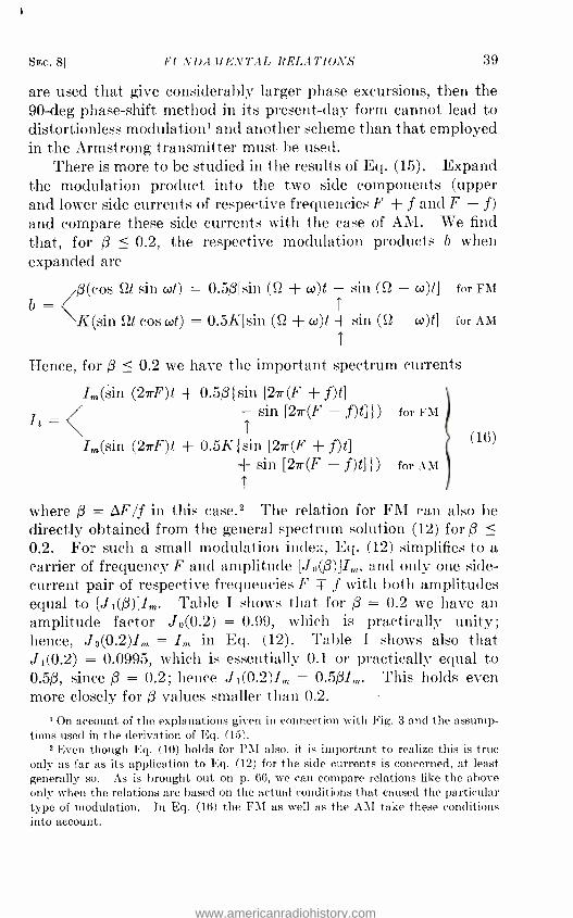
SEC. 8] FUNDAMENTAL RELATIONS 39
are used that give considerably larger phase excursions, then the 90 -deg phase -shift method in its present-day form cannot lead to distortionless modulation' and another scheme than that employed in the Armstrong transmitter must be used.
There is more to be studied in the results of Eq. (15). Expand the modulation product into the two side components (upper and lower side currents of respective frequencies F + f and F - f) and compare these side currents with the case of AM. We find that, for ß <_ 0.2, the respective modulation products b when expanded are
ß(cos Slt sin wt) = 0.50[sin (Sl + w)t - sin (S2 - w)t] for FM
b =<K(sin IN cos wt) = 0.5K[sin (S2 + w)t + sin (St - w)t] for AM
T
Hence, for ß <_ 0.2 we have the important spectrum currents
Im(sin (2irF)t + 0.50{ sin [2ir(F + f)t] - sin [21r(F - f)t] {) for FM
T
Im(sin (2irF)t + 0.5K {sin [2ir(F + f)t] + sin [2r(F -f )t] {) for AM
T
where ß = AF /f in this case.' The relation for FM can also be directly obtained from the general spectrum solution (12) for /3
0.2. For such a small modulation index, Eq. (12) simplifies to a carrier of frequency F and amplitude [Jo(ß)]I and only one side - current pair of respective frequencies F -T f with both amplitudes equal to [J1(3)]Im. Table I shows that for ß = 0.2 we have an amplitude factor J0(0.2) = 0.99, which is practically unity; hence, Jo(0.2)Im = Im in Eq. (12). Table I shows also that J1(0.2) = 0.0995, which is essentially 0.1 or practically equal to 0.5ß, since ß = 0.2; hence J1(0.2)Im = 0.50,. This holds even more closely for ß values smaller than 0.2.
1 On account of the explanations given in connection with Fig. 3 and the assump- tions used in the derivation of Eq. (15).
2 Even though Eq. (10) holds for PM also, it is important to realize this is true only as far as its application to Eq. (12) for the side currents is concerned, at least generally so. As is brought out on p. 66, we can compare relations like the above only when the relations are based on the actual conditions that caused the particular type of modulation. In Eq. (16) the FM as well as the AM take these conditions into account.
It = (16)
www.americanradiohistory.com

40 FREQUENCY MODULATION [CHAP. I
Equation (16) is important since it shows that for a modulation index OF /f = 0.2, or smaller, FM behaves exactly like AM as far as the spectrum distribution is concerned. In addition, we can now consider the modulation index ß as equivalent to a modulation factor. The amplitude of the carrier current of frequency F, whether due to FM or to AM, remains equal to the carrier level
We also note that practically all of the modulation energy for FM exists only in the side bands. Even though for AM the modulation energy rests likewise in the only and first side -current pair, Eq. (16) shows that for AM both the upper and the lower side currents are characterized by positive amplitudes, which
I=Im 1.0- K=100 %
0.8-
T 0.6 -
0.4 -
F
Experimental Ke -curve
-f-- --' +f FIG. 1M.- Experimental curves for the first side -current pair of frequencies F -f and F -}- f
(for different signal frequencies f).
are the same and equal to 0.5KIm. But, for FM, the amplitude of the side frequency F + f is plus 0.50I; the amplitude of side frequency F -f is minus 0.5ßIm. Hence, when FM and AM act simultaneously, there must be a signal frequency fi for which ß = AF/fi becomes equal to K and the lower side current vanishes. This is indicated in Fig. 16. Since, according to Eq. (16), on the upper side -band side both AM and superimposed FM effects are additive, the effective upper side -current amplitude is no longer 0.5KI,, as would be expected if AM only were present, nor (0.5AF, fi)/m, as would be expected if pure FM prevailed. But we find an effective upper side -current amplitude Iu = 0.5KI , -1-
0.50Ií, which expression can also be written as Iu = 0.5KeIm if the effective modulation factor for the upper side band is taken as Ke = K +13. For the lower side band it would be Ke = K -ß
www.americanradiohistory.com

SEC. 8] FUNDAMENTAL RELATIONS 41
Hence, at this particular modulating current of frequency f,, we have automatic lower side- current suppression, as far as a side
frequency F - is concerned. In Fig. 16 the unmodulated carrier level /in is assumed equal to
unity. Hence, the respective side- current amplitudes for various signal frequency values are given by the respective Ke charac- teristics. Such a superposition of two kinds of modulations is generally not desirable since the lower side -current amplitude characteristic behaves differently from the upper side -current amplitude. In other words, it is essential that we avoid a parasitic modulation of the undesired type. It is true that a detector of
AM by itself does not respond at the output side to FM. But when, as is shown in Fig. 16, the effective modulation factor Ke has,
so to speak, "all the characteristics of AM" then the AM detector will respond accordingly. This will produce distortion at its
output and, therefore, a -f distortion. For useful FM acting with
parasitic AM, we must realize that any FM -AM translator is not
exactly immune to AM. All demodulators must depend on some
function of the amplitude; otherwise they could not give zero out- put when zero amplitude is impressed. Fortunately, this is of
no practical consequence, since we use at least one stage of ampli-
tude saturation, or limitation as it is called, ahead of a frequency discriminator. This limits the amplitude applied to the dis-
criminator enough to cut out variations of amplitude. In connection with Fig. 3, it was already mentioned that even
the geometrical quadrature addition of the modulation product with the unmodulated carrier produces, besides the desired PM,
also amplitude variations; i.e., it produces undesirable superim-
posed AM. But by " clipping off," the by- product of AM is
avoided in succeeding stages. Limiters are therefore essential
apparatus, in FM work. Whatever undesirable AM is produced in a transmitter should be corrected right in the transmitter and,
if possible, right at the place where it sets in. In a receiver,
two limiter stages seem desirable. They should precede the
discriminator. Since the Ke curve of Fig. 16 on the lower side -band side passes
through zero at a critical modulation frequency f = f,, we have a
means for finding either the value of K, if the value ß for FM is
known, or the modulation index ß if the condition of AM is known.
Since the critical frequency fi can be determined, for instance, by
www.americanradiohistory.com
42 FREQUENCY MODULATION [CHAP. I
means of the calibration of a beat frequency oscillator, we can find then also the value of the maximum frequency excursion F. For the critical frequency f 1, the determinations just described are based on the equality K = AF/fi when the lower side current vanishes. Consider FM as the desired type of modulation. If we find by means of a search -current method' that the lower side - current amplitude disappears' at a frequency fi = 4 kc and the maximum frequency excursion is known to be OF = ±0.8 kc, then we have a modulation index ß = 0.8/4 = 0.2 and the unde- sired AM has a modulation factor K of 20 per cent.
It should be noted that this experimental method applies also for cases where the modulation index has almost any value3 since according to the distribution equation (12) instead of the factor 0.513 we have to take the associated Bessel factor J,(ß) into account. The first lower side current disappears for a ß = OF /f 1 value which makes J1(0) = 0.5K instead of 13 = K.
On the other hand, if the degree of AM is known, that is, if
AM is the desired modulation and K = 0.2 as in Fig. 16 and the lower side -current amplitude disappears at a frequency of 150
cycles per second, we have AT = OF /150 = 0.2. Hence, in this case the maximum frequency swing ¿F, due to parasitic FM, would be ±30 cycles per second. For the case where a 10 -ke signal frequency causes disappearance of the first lower side - current amplitude, we would have a maximum frequency swing OF = ±0.2 X 10,000 = ±2 kc. If larger 13 values than 0.2
exist for parasitic FM, the above relation for which J1(ß) is equal to 0.5K is to be used in the computation. Larger values will,
however, be unlikely to occur for parasitic modulations since
a network would normally not be so poorly designed. 9. Three Types of Modulation. -As to AM, it is evident that
the instantaneous value of the carrier frequency F remains con-
stant. Since an FM as well as a PM current has the form Im sin (SZt + ß sin cat) for the instantaneous current value, the argu-
I Consult "High- frequency Measurements," pp. 116 -126, 377 -381. 2 For simultaneous FM and AM only the first lower side current disappears at the
critical frequency f,, but never the amplitude of carrier frequency F. Therefore, we
should never use, in the method for determining of by means of Bessel curve inter-
sections (see p. 86), the intersection of the J,(R) curve since the zero amplitude condition could be entirely or partly due to a parasitic superimposed AM, instead of
to the disappearance of the J,(R) value. a For details see p. 70.
www.americanradiohistory.com

SEC. 9] FUNDAMENTAL RELA1JII_V,5 43
ment in the parenthesis must denote the instantaneous angular
velocity SZ,. The instantaneous frequency F, of the carrier fre-
quency is S2r /(27r) or
1 d(SZt + ß sin wt) cóß cos cot I't = 2,r dt 2r
where for FM we have ß = iF /f and for equivalent FM, i.e., PM,
we have ß = AO. Therefore,
F + OF cos wt
Fr = F+fOB cos cot
true FM
PM (which is equivalent FM)
(17)
showing again that for PM the equivalent frequency swing
depends, even for a fixed maximum phase swing AO, on the signal
frequency f also, since the equivalent maximum frequency excur-
sion is f O. At this point it should be understood that an FM -AM
translator will respond to either PM or FM voltages as far as the
a -f effects in the AM output' current are concerned. For this
reason, distortion in FM receivers often can be due to undesirable
PM effects. It is of utmost importance, therefore, that transfer
networks, especially those used in the i -f stages, be designed for a
linear phase shift with respect to all frequencies concerned in the
band width. Figure 17 shows AM in comparison with FM. The modula-
tion cycle can be readily seen in the AM representation. The
line density in the representation for FM (similar to sound rarefec-
tions and condensations) indicates the modulation cycle. The
respective spectrum distributions show that in the case of AM the
modulation energy never affects the amplitude of carrier frequency
F, while for FM the modulation energy is spread over the entire
frequency spectrum. This is, of course, also true for PM since
for a particular signal frequency f we have, according to Eq.
(17), a maximum frequency deviation f M, which can have the
same order as a true frequency swing M'. In FM and in PM,
the modulation effect on the amplitude of carrier frequency F
always causes a decrease in this amplitude, even though extremely
In commercial frequency discriminators the output gives usually the a -f current.
This means that inherent amplitude demodulation takes place in the discriminator.
Hence such a discriminator should actually be called an FM -AM audio con-
verter. For such discriminators the audio current at the output terminals is due
to either FM or PM affecting the input of the discriminator.
www.americanradiohistory.com
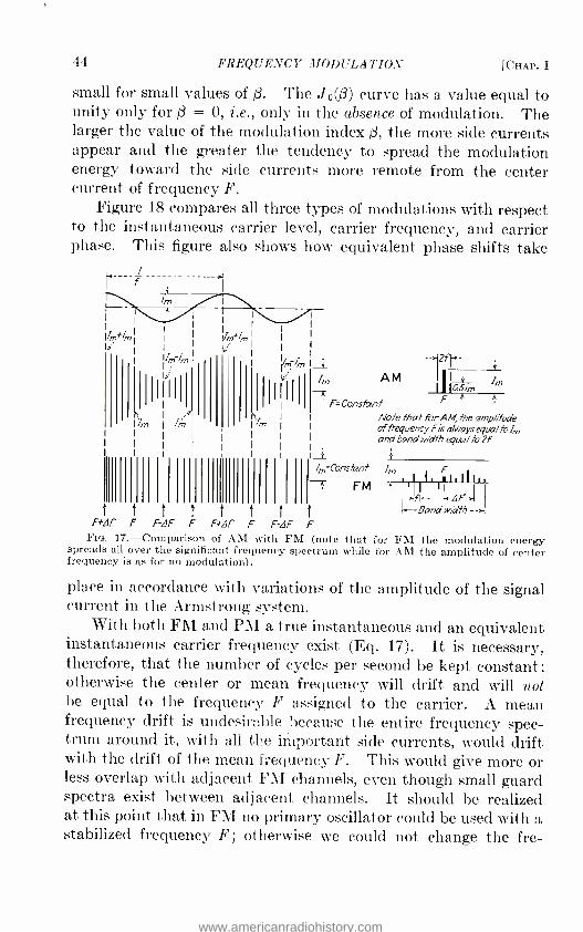
44 FREQUENCY MODULATION [CHAP. I
small for small values of ß. The J0(0) curve has a value equal to unity only for ß = 0, i.e., only in the absence of modulation. The larger the value of the modulation index ß, the more side currents appear and the greater the tendency to spread the modulation energy toward the side currents more remote from the center current of frequency F.
Figure 18 compares all three types of modulations with respect to the instantaneous carrier level, carrier frequency, and carrier phase. This figure also shows how equivalent phase shifts take
I 7
A
Id
Im
III I,n AM
I
I F=Constant
t t t t t t t F +dF F F-OF F F+dF F F -. F F
FIG. 17.- Comparison of AM with FM (note that for FM the modulation energy spreads all over the significant frequency spectrum while for AM the amplitude of center frequency is as for no modulation).
place in accordance with variations of the amplitude of the signal current in the Armstrong system.
With both FM and PM a true instantaneous and an equivalent instantaneous carrier frequency exist (Eq. 17). It is necessary, therefore, that the number of cycles per second be kept constant: otherwise the center or mean frequency will drift and will not be equal to the frequency F assigned to the carrier. A mean frequency drift is undesirable because the entire frequency spec- trum around it, with all the important side currents, would drift with the drift of the mean frequency F. This would give more or less overlap with adjacent. FM channels, even though small guard spectra exist between adjacent channels. It should be realized at this point that in FM no primary oscillator could be used with a stabilized frequency F; otherwise we could not change the fre-
Im
Note That for AM, the amplitude of frequency fis a /ways equal to and band width equal to 2f
c 4
I,, =Constant ¡, F
,}rl IIit. FM °
Ith- rl.aF-I I
--Sand width --I
www.americanradiohistory.com

SEC. 9] FUNDAMENTAL RELATIONS 45
quency directly during the modulation cycle and produce FM. But with PM the frequency can be stabilized since the equivalent frequency change is due to phase fluctuations.
FM
PM
AM
Variab /emcarrier frequency Ft
r7 4= la,sin[2rrFt +% sinl2irft)] 2l Ft= F +dFcos(2rrfi9 .. true frequency
lm level remains constant modulation index /3=7 F
Fixed carrier frequency F ,variable phase
lJ= /msin[2 rFt +de sin (1n ft)) Bt = B +d 8 sin (2rr ft).... true relative phase F =F +f.69.0s(2rrftl... apparent or
equivalent frequency Im level remains constant Modulation index /4 =48
seconds
+dB/f, t1
21n, i i1
i i i1
i i
14 1
lt=lm[l +Pmcos(2rrftgsin(2rrFt)
7 Carrier frequency Fl J remain constant
21 Relative phase B Carrier level In t =la [l+ m cos (2rrft)J
Modulation factor K= m
i7 ! 27m
1
Signal voltage of frequency f of balanced modulator
APPARENT PM Armstrong's modulated current with maximum phase liberations of á f ¡9 =
In, and F remain constant apparent Ft= F+ f cos (27rft)
= F +dB cos (2rrft) et =B+ f sin (2rrft)
FIG. 18.- Comparison of direct FM, direct PM, AM, and indirect FM.
With respect to the effective current value I of a modulated current, we have according to Eq. (1), the formula
1 2r I= 271- J Im sin2 (27rFt + B) dt (18)
For AM we have instead of Im the value I,(1 + K cos cot) and the fixed relative phase O is neglected since it has nothing to do with AM. Making these substitutions, we have
= V 1
f - I (1 + K cos wt)2 sin2 S2 dt = 1.41 A/1 0.5K2 (19)
in contrast with the value I ,.; 1.41 for the unmodulated carrier.' 1 For details consult "High -frequency Measurements, pp. 361 -362.
www.americanradiohistory.com

46 FREQUENCY MODULATION [CHAP. I
Even though it looks evident that for pure FM, as well as for PM which gives equivalent FM, the effective value is the same as for the unmodulated current, it may be of interest to understand the proof of it.
Since for both FM and PM, the instantaneous current value has the form Im sin [27rFt + ß sin (27rf)t], we have for the effective current value the formula
1 ° I = 2- J Iñ, sine [271-Ft + ß sin (27rf)t] dt (20)
For any type of signal current and any type of modulation, we have generally the formula
an
I = 2
1 71- J Ir dt (21)
The evaluations of Eq. (20) for either PM or FM, depending on whether ß = M or is equal to OF /f, are laborious. Fortunately, the evaluation can be made very simple if only harmonic com- ponent currents play a part, even though they may have no integer relationship with respect to each other.
We know from alternating- current theory that the funda- mental and all higher harmonics in a distorted current wave are added geometrically to obtain the effective resultant current value as is indicated by a thermoelectric ammeter, for instance. Now, our spectrum solution in Eq. (12) gives us the amplitude as well as the frequency of all the sinusoidal currents. Even though not in harmonic relationship, we have also to deal with geometrical addition if we want to find the effective current value. In this manner involved integration, as indicated in Eqs. (20) and (21), is avoided. Since in Eq. (12) the amplitudes of the different spectrum currents denote maximum amplitude values, these values must be divided by 1.41 in order to obtain the corresponding effective component values. Therefore, we have for the effective value of an FM or PM current
I = 1.41 1 J2(0) + 2,I;.(0) + 2Jz(0) + 2Já(ß) + . (22)
where ß = 07+' j f for FM, or ß = M radians for PM. The numeri- cal value will then take care of the degree of the respective modula- tion. The factor 2 appears in all Bessel factors belonging to the
www.americanradiohistory.com

SEC. 9] FUNDAMENTAL RELATIONS 47
side -current pairs since, for instance, for the first side -current pair an effective value J,(ß)I,n /1.41 of frequency F -f has to be added geometrically to the effective component value J,(0)Im /1.41 of frequency F + f in order to account for the resultant effective current of the entire pair. The addition has to be made geome- trically (square root of the sum of the squares) since these two components are of different frequencies.
Now with a knowledge of the value of ß, Bessel tables or curves show how many terms have to be used and the effective value I can be computed quickly. For instance, for a value of ß = 0.2 we have only the first side -current pair in addition to the current of carrier
frequency F. Hence I = Im/1.41 -4(0.2) + 2 X 4(0.2) =
(Im /1.41) 1/1 + 2 X 0.12 = (Im /1.41) - /1.02. Since, according to Table I, the exact values of J0(0.2) = 0.9975 and J1(0.2) = 0.0995, we note that I = Im/1.41. This result could also be
obtained from Eq. (16), which shows that for ß <_ 0.2 we have
I = (/,/ 1.41) A/1 + 2 X 0.5202 or I = le -V1 + i2ß2 where le
denotes the effective current value of the unmodulated carrier. We see that 1 + i2132 = 1.02 as above. If no approximations had been made, i.e., if all side currents, even the smallest ones, had been taken into account, the result would have been exactly equal
to unity. Hence, we see that such a checkup will disclose whether we have missed important side currents.
Suppose that we have a case where the modulation index is
ß = 5. This is, for instance, the value for the maximum deviation ratio for wide -band FM since for OF = ±75 kc and the highest signal frequency fm = 15 kc this ß value obtains. Our Bessel
tables show that about eight side -current pairs play a part. The
tables give the following values: J0(5) = 0.1776, J,(5) = 0.3276,
J2(5) = 0.0466, J3(5) = 0.3648, J4(5) = 0.3912, J5(5) = 0.2611,
J6(5) = 0.131, J7(5) = 0.0534, and J8(5) = 0.0184. All values
are written down without respect to polarity since it is not needed
here. The sum under the square -root sign of Eq. (22) then
becomes 4(5) + 24(5) + 2J2(5) + 2J3(5) + 24(5) + 2J5(5) + 2J6(5) + 24(5) + 2J8(5) = 0.0315 + 0.214 + 0.0044 + 0.266 + 0.306 + 0.136 + 0.0342 + 0.0056 + 0.00068 = 0.99838, which is
again essentially unity. For FM as well as PM, the effective current reading should be
the same as the value of the unmodulated carrier current, unless
www.americanradiohistory.com

48 FREQUENCY MODULATION [CHAP. I
the network in which the reading is taken or the network that carries the FM or PM current cannot pass without amplitude, frequency, or phase discrimination all the important side currents. The ammeter method can, therefore, be used to test the pass -band property of FM and PM networks. If a different current reading is obtained for no modulation or for any degree of FM or PM, the network requires a better design. But an increase of current, when measured with an rms ammeter, may be due to superimposed parasitic AM. To find out whether this is the case, the method described on pages 40 and 63 should be employed before cor- recting a transfer network.
Equation (19) has exactly the same form for FM and PM when ß < 0.2, if the amplitude modulation factor K is replaced by the modulation index ß. Nevertheless, there is a great difference between this expression with K and when ß is used instead of K. This is due to the fact that ß can be used only for values of ß = 0.2 or smaller. For such values of ß, Eq. (19) yields an effective modulated current value that is essentially equal to the effective value of the unmodulated current for AM, FM, and PM. For values of ß larger than 0.2, the index ß should not be used in Eq. (19). However, the equation is correct with K values for any possible value of K. For instance, K = 1 means that im = I,,,, or that 100 per cent AM exists and Eq. (19) would yield an effective current value that is 1.2247 times larger than the effective value of the unmodulated carrier current.
Since in the spectrum distribution for large values of ß most of the modulation energy spreads toward the side frequencies farthest away from the carrier frequency F, it is seen that sharp cutoffs are required in the band -pass design of FM networks. It is true that for the smaller values of ß not so many side currents occur. But with a fixed maximum value of AF = ± 75 kc the smaller values of ß occur only for the highest desired signal fre- quency. This frequency is usually taken as 15 kc. Hence, even though not so many important side currents occur, on account of
the large value of the signal frequency f, the band spread becomes widest for these small values of ß when the highest permissible modulation degree is being used. Inasmuch as we have to deal with all the important signal frequencies, it is the value of OF = ± 75 kc and the value of f = 15 kc that determines the required band width. If a sharp cutoff band -pass network cannot eco-
www.americanradiohistory.com

SEC. 10] FUNDAMENTAL RELATIONS 49
nomically be designed, the network should be designed for a band -pass region sufficiently wide so that the essential band width required by the spectrum distribution is properly accommodated. Such an additional band width is, in addition, favorable in regard to the signal -to -noise ratio.
10. Addition of Modulation Products. -In the case of AM, the unmodulated carrier level is equal to the amplitude Im of the unmodulated carrier current. For FM, the unmodulated or normal carrier level is the carrier frequency F, which is also often called the mean or center frequency. Even though for PM we could call a certain fixed phase O the normal level, we may also here refer to the carrier frequency F as the normal level since we have in effect equivalent frequency deviations about the fixed carrier frequency F.
At this point it may be of value to realize that a different instantaneous frequency Ft in case of FM means that the fixed carrier frequency F has changed to a value that at the instant t is Ft. For PM, which causes equivalent FM, the fixed carrier frequency F remains fixed but the PM reflects, so to speak, a superimposed carrier frequency deviation on the fixed value of F. In equivalence this gives also an apparent instantaneous frequency Ft, which differs from F. In each case, i.e., for FM as well as PM, the variations about the mean frequency F are registered at the output of a frequency discriminator since this device responds to frequency swings.'
In connection with Fig. 5, for AM it has been seen that the modulation product b is always in phase with the normal carrier level a, which is equal to Im. Hence, in AM we have only to deal at any instant with algebraic additions, a + b, or subtractions, a - b, depending on whether the magnitude KIm cos wt in the
We have, therefore, a parallel with the actions of a coil when used over a wide frequency range. A coil remains a coil, hut in equivalence it acts above its natural resonance like a condenser since the coil capacitance action outweighs the inductive action. It takes then a small coil with little distributed capacitance to tune to a still higher frequency. With PM we still have the fixed F no matter how much degree of PM exists, hut as far as the equivalent frequency deviations about the fixed F and their effect on the discriminator are concerned, it would require an FM deviation of the saine . /' hut instantaneously in exact opposition to neutralize the frequency- variation effect due to PM. In other words, the equivalent variation f AO cos cut has to be opposed by a true carrier- frequency change -LIF cos wt and such that at any instant of the modulation cycle, AF, = f SO,. This can be readily done for one particular frequency but only with a corrective network for the entire hand.
www.americanradiohistory.com
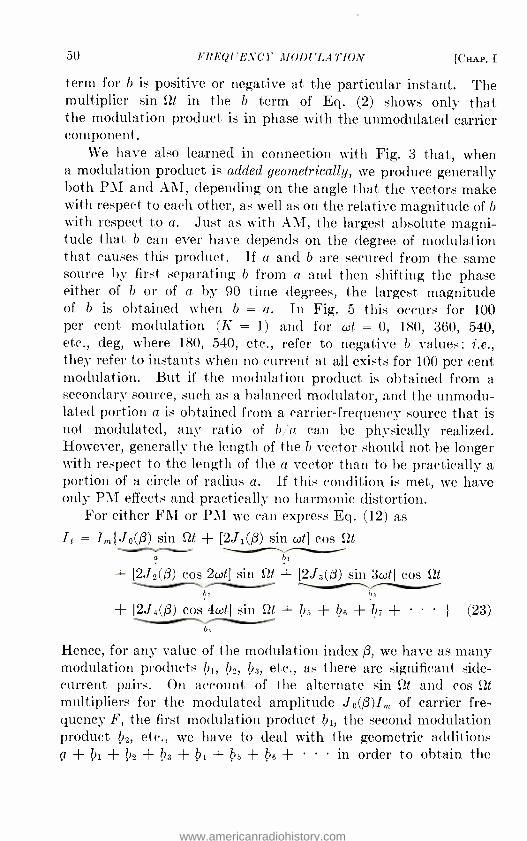
50 FREQUENCY MODULATION [CHAP. I
term for b is positive or negative at the particular instant. The multiplier sin Sgt in the b term of Eq. (2) shows only that the modulation product is in phase with the unmodulated carrier component.
We have also learned in connection with Fig. 3 that, when a modulation product is added geometrically, we produce generally both PM and AM, depending on the angle that the vectors make with respect to each other, as well as on the relative magnitude of b
with respect to a. Just as with AM, the largest absolute magni- tude that b can ever have depends on the degree of modulation that causes this product. If a and b are secured from the same source by first separating b from a and then shifting the phase either of b or of a by 90 time degrees, the largest magnitude of b is obtained when b = a. In Fig. 5 this occurs for 100 per cent modulation (K = 1) and for wt = 0, 180, 360, 540, etc., deg, where 180, 540, etc., refer to negative b values; i.e., they refer to instants when no current at all exists for 100 per cent modulation. But if the modulation product is obtained from a secondary source, such as a balanced modulator, and the unmodu- lated portion a is obtained from a carrier -frequency source that is not modulated, any ratio of b% a can be physically realized. However, generally the length of the b vector should not be longer with respect to the length of the a vector than to be practically a portion of a circle of radius a. If this condition is met, we have only PM effects and practically no harmonic distortion.
For either FM or PM we can express Eq. (12) as
It = /,,{J0(0) sin Sgt + [2J1(ß) sin wt] cos SZt . a bi
+ [2J2(ß) cos 2wt] sin Qt + [2J3(0) sin 3wt] cos Sgt
b. ba
+ [2J4(ß) cos 4wt] sin Sgt + b; + N + b7 + b4
Hence, for any value of the modulation index ß, we have as many modulation products bl b2, b3, etc., as there are significant side - current pairs. On account of the alternate sin Qt and cos Qt multipliers for the modulated amplitude Jo(ß)I,,,, of carrier fre- quency F, the first modulation productbl, the second modulation product b2, etc., we have to deal with the geometric additions a+bi+b2+63 +64 +b5 +b6+ in order to obtain the
(23)
www.americanradiohistory.com

SEC. 10] FUNDAMENTAL RELATIONS 51
vector of the resultant current It at any instant. The addition is, therefore, in quadrature between consecutive modulation products or modulation factors bí, b2 1)3j etc., as well as with respect to the vector á of carrier or center frequency F.
It should be clearly understood that for either FM or PM, which differ in the spectrum solution only in that for FM the index ß = AF j f and for PM the index ß = M, the amplitude of the carrier frequency F is also affected for such quadrature modulations, i.e., modulations along the time. axis. This is especially so for large values of O. However, it is not due to any one component modulation product, but to the effect of all the modulation products belonging to the respective side -current pairs. In other words, the modulation energy distributes itself over all of the frequency spectrum that is of practical importance. For the larger values of ß so much energy is diverted toward the side bands on each side of the carrier frequency F that a carrier amplitude Jo(ß)I,, which is smaller than Im, results; i.e., this diverting of energy to the side bands even takes along some of the normal carrier power. As a matter of fact, the energy distribution in the important spectrum portion of the spectrum due to noise or other erratic interference is not so effective as the energy dis- tribution resulting from FM or PM in producing a response in the demodulator of a proper type of receiver. Hence, the desired intelligence in FM or PM will, so to speak, "outweigh" any noise that causes random energy distributions. The Bessel energy distribution is, therefore, one of the outstanding features of FM as compared with AM. These features are, of course, also true for PM.
The simplest application of Eq. (23) occurs when ß <_ 0.2 since then only the á and bí vectors have significant values. We have then a simple vector addition in quadrature, as shown in Fig. 3. From Table I we note that for such ß values the Bessel factor J0(-0.2) is essentially equal to unity. Hence, the length of vector is equal to Im. Now if we take the case for ß = 0.2, we find Jí(0.2) = 0.0995, which is essentially equal to 0.1, or 0.5ß. The length of the vector representing the modulation product bí is then bí = 2J1(0.2)Im sin wt = 0.2I,n sin wt. As a matter of fact, the formula bí = ¡Im sin wt holds for all ß values smaller than 0.2 and Bessel tables are not needed. The only significant modulation vector bí has then an absolute length
www.americanradiohistory.com

52 FREQUENCY MODULATION [CHAP. I
b1 = 0.2Im at the instant of time when wt = 90 deg; i.e., at the instant when the modulation cycle just reaches the first positive maximum frequency excursion +OF in case of FM. Hence, as shown in Fig. 3, we add to the vertical vector a of length a = Im, the vector bi of length b1 = 0.21m in time quadrature and along the positive direction. Now if we assume that the time is such that wt is equal to 225 deg, then sin 225 = - sin 45 = -0.7071 and b1 = -0.707 X 0.2Im = -0.14142I, . Hence, the vector bl of length -0.141421m is to be added, in quadrature and in the negative direction, to vector g, of length Im. Since Jo(0.2) is strictly equal to 0.99 and J1(0.2) = 0.0995, we find for wt = 90 deg that a = 0.99Im and b1 = 0.199Im and that for wt = 225 deg the exact value of b1 = - 0.7071 X 0.199Im = -0.14061m. For wt = 0, 180, 360, 540, etc., deg the modulation term b, vanishes and only the term a = 0.99Im remains to account for I,. The result- ant value or vector corresponding to le has, for the instant when wt = 90 deg, the value Igo = I, .V0.992 + 0.1992, which is essentially equal to Im. For wt = 225 deg we have 1225 = Im /0.992 + 0.14062, which is again essentially equal to Im. This means that for the entire signal cycle of frequency f, the resultant current has the constant amplitude level Im. The small differ- ences between the actual square -root values and the theoretical value of unity is caused by the fact that the less significant terms were neglected in obtaining the square -root values. These differences become still more pronounced for somewhat higher ß values if we add only the first modulation vector bl in quadrature with a, since actually the vector V2 should be included also. The effect of neglecting the higher modulation products for ß = 0.5 radian or 0.5 X 57.3 = 28.65 deg in PM is that during the signal or modulation cycle the resultant vector V'a2 + bi fluctuates for different wt values and we have a small degree of AM in our calcula- tions.
Suppose we have now to take into account more modulation products due to a larger value of ß, such that more side -current pairs play an important part. Matters are then no more difficult, as the following numerical example and the vector diagram of Fig. 19 will show. The successive quadrature addition of á, b2j 3, b4, etc., for significant b terms satisfies the relation It = Im sin (Qt + )3 sin wt). This holds for respective spectrum dis-.
www.americanradiohistory.com

SEC. 101 FUNDAMENTAL RELATIONS 53
tributions for either FM or PM, depending on whether ß = AF /f or ß = O. Hence, all resultant current vectors for various values of time must have essentially the same absolute length and be equal to In, since the foregoing expression causes a circular trace. The spectrum equation (23) also must yield a circle of radius Im
if sufficient modulation products are included. The resultant vector IL then spins around with an instantaneous angular velocity 0, which is equal to 6.28[F + OF cos (27rf)t] in case of FM; for PM it is equal to 6.28[F + f A9 cos (27rf)t], where M is to be expressed in radians; i.e., it must be numerical. Hence, in each
` 63=0034 /,n
62 b2 =0/761,n
á b, =0.88021,n b,= 0.301Im
ti I E
ON + ( a +b
h 2 v-
b3 =- 003921m it
wt= 90° wt =0° wt =20°
(a) (b) (c)
FIG. 19.- Graphical proof that the resultant current If has always the same carrier level L .
case the resultant current vector spins around with the apparent constant angular velocity 6.28F, but at the same time it is exposed to angular velocity increase and decrease "flutters" at the signal - frequency rate. The instantaneous angular velocity deviations from the mean constant angular velocity 6.28F are given by 6.28 OF cos wt for FM and by 6.28f M cos wt for PM, where w = 6.28f.
Assume a modulation index ß = 1. Table I shows that for this case three significant modulation products play a part. Hence, the magnitude of the resultant current vector is -V (a + b2) 2 + (b1 + b3) 2
since successive quadrature additions must be made. Therefore, the odd terms are in phase, just as the even terms, a, b2, b4, bs, .. are in phase.
At this point it is of importance to realize that the polarity of the Bessel factors plays a part since a negative Bessel value will
www.americanradiohistory.com

54 FREQUENCY MODULATION [CHAP. I
cause opposite polarity of the vector to be added. Of course, the harmonic modulation function wt also affects the polarity.
From Table I the Bessel factors are J0(1) = 0.7652, J1(1) = 0.4401, J2(1) = 0.1149, and J3(1) = 0.0196. Hence, according to Eq. (23), the current of carrier frequency F has, at any time of the modulation cycle, a constant scalar value Jo(1)Im = 0.7652, = a. For the first modulation product we have the instantaneous scalar value b1 = 2J1(1)Im sin wt = 0.88021m sin wt. For the sec- ond modulation product we have the instantaneous scalar value b2 = 2 X 0.1149/, cos 2wt = 0.22981m cos 2wt. For the third modulation product we have the instantaneous scalar value b3 = 0.03921, sin 3wt. Hence, at an instant of time, when wt = 20 deg, for example, we have a = 0.76521m; b1 = 0.8802/, sin 20 deg = 0.8802 X 0.3421, = 0.3011m; b2 = 0.22981, cos 40 deg = 0.2298 X 0.7661m = 0.1761m; and b3 = 0.03921, sin 60 deg = 0.0392 X 0.8661m = 0.0341m.
We have, therefore, the vector addition shown in Fig. 19e, which by graphical construction confirms the value of the resultant as equal to Im. We can also find the resultant from
V(a + b2) 2 + (b1 + b3) 2 Im = Im 0.94122 + 0.3352
= Im0.997 =Im.
For wt = 0 deg, we have the case of Fig. 19b and the values a = 0.76521m, b1 = 0, b2 = 0.22981,, and b3 = 0. We obtain, therefore, a resultant current value a + b2 = 0.76521m + 0.2298/m = 0.9951m, which is again essentially equal to Im. For wt = 90 deg we have the vector display of Fig. 19a and the following computa- tions: a = 0.76521m, b1 = 0.88021m, b2 = - 0.22981m, and b3 =
0.03921m. Therefore, a + b2 = 0.76521m - 0.22981m = 0.53541, and b1 + b3 = 0.88021m - 0.0392/, = 0.8411m. Hence, the result- ant current is Im Y0.53542 + 0.8412 = Im Y0.992, which is likewise essentially equal to /m, as should be the case. Hence, the number of modulation products chosen shows that essentially no undesired AM effects will be superimposed if the band -pass networks will accommodate or pass the three side -current pairs, since the carrier level remains essentially constant and equal to Im.
From these numerical speculations some important conclusions may be drawn. For modern commercial wide -band FM, for the highest signal frequency at full permissible OF' swing, the 0 value is equal to about 5. According to Table III,
www.americanradiohistory.com

SEC. 11] FUNDAMENTAL RELATIONS 55
for ß = 5 we have eight significant side -current pairs; that is, eight modula- tion products, and can expect more or less pure FM. When indirect FM is produced by means of only one modulation product, the corresponding modu- lation vector should never be permitted to reach a maximum value large enough to produce a ß value exceeding a value of 0.2. If, as in some commercial work, 0 values as high as 0.5 radian are tolerated, the small superimposed AM should be "clipped off" with an amplitude limiter. It is true that even in modern direct FM the value of ß = 5 for the highest signal frequency of about 15 kc holds only for the maximum permissible modulation condition in the final stages of an FM transmitter, since at least a several fold frequency multiplication is
employed after the so- called "primary" FM is effected. The frequency multi- plication is customarily accomplished with ordinary receiver tubes, as far as their power rating is concerned at least. Hence, the primary OF swing is not ± 75 kc, but is as many times smaller as the value of the frequency swing multi- plication factor. For an eightfold frequency multiplication the primary AF swing is, therefore, only 75/8 kc and the corresponding ß value for a maximum frequency deviaton ratio of 5 is only 5/8 for the primary FM. Hence, the circuit design requires more band width after the swings are multiplied, since ß increases accordingly on account of an increase in the value of F. The value off in the expression ß = OF /f cannot change with the frequency multiplication, since it accounts only for the speed with which the AF swings occur, and controls the pitch of the sound heard at the receiver. For weaker modulation degrees, i.e., for less intense intelligence transmission, the ß value becomes smaller. Then the number of corresponding side currents produced can surely be accommodated, since the band width is designed for the maximum deviation ratio 75 kc/15 kc = 5.
11. Effects When Two Types of Modulations Are Present. -It is not uncommon to have AM associated with PM or FM. The reason for this is that any circuit reactions may produce unde- sirable PM, even in circuit elements between the antenna and the last power stage. Any reactive back actions on the master oscillator of an AM system will cause direct FM effects unless the source of the carrier frequency is perfectly stabilized. In connection with Fig. 3, as well as in the discussion in Sec. 10, it was noted that undesirable AM effects may appear in FM or PM systems unless these effects are clipped off. It is now of interest to examine what happens when two types of modulation occur simultaneously in a system.
In another publication' the general solution for the instantane- ous value of a modulated current when two types of modulation are present simultaneously is given. If we neglect the constant phase in Eq. (23) of this reference, we have the simplified general solution
"High- frequency Measurements," p. 376, Eq. (23).
www.americanradiohistory.com

56 FREQUENCY MODULI.] l()\ ¡('1.11'. 1
M, M,
It = Im(1 + K sin wt) [sin (SZt + ß sin wt)]
= Im (J.(ß) Sin (SZ + nw)t
- 0.5KJn(13) cos {[S1 + (n + 1)w]t1
+ 0.5KJn (ß) cos {{ S2 + (n - 1) w]t }) (24)
The driving voltage in a load circuit coupled to an AM source causes a h -f current flow in that circuit, which is directly propor- tional to the induced driving voltage. Experience has shown that tanks as well as open -circuit loads' may cause a certain phase shift, in the modulated current flow, which, in turn, means that this phase shift must be also a linear function of the driving voltage. For a sinusoidal modulating voltage, the phase O in Eq. (1), as well as its amplitude Im, must also vary sinusoidally. Hence, in Eq. (1) instead of Im we have the sinusoidal amplitude variation (1 + K sin cot)/na and instead of O we have the sinusoidal phase variation M sin wt. The equation for the resultant current then reads
It = Im(1 + K sin wt) sin (Qt + M sin wt)
Since, in PM, the maximum phase swing M = ß, Eq. (24) applies. This equation shows that we have now two modulation opera-
tors: M1j which causes AM, and M2, which causes PM. The expression It = M1M2Im shows that, as far as the envelope or amplitude contour of the doubly modulated current is concerned, the term M2 can have no effect on the contour. M2 causes quad- rature actions only; i.e., it causes effects along the time axis of the modulated current wave, but no effects along and parallel to the amplitude axis. These statements are correct for the load circuit, but matters are different at the reception end. Equation (24) shows that the complete modulation energy is no longer in the first and only modulation product, as in case of pure AM, but is all over the significant frequency spectrum if undesired PM is also present. Hence, all networks, including the antenna branch, have to be designed to accommodate the wider required frequency spectrum. Since the term M2 in the spectrum solution of Eq. (24) causes quadrature effects as far as the various h -f currents result- ing from the spectrum distribution are concerned, the rotating
' A transmitter antenna is, for instance, an open- circuit load.
www.americanradiohistory.com

SEC. 11] FUNDAMENTAL RELATIONS 57
vector representing the instantaneous position of the twofold modulated current It will no longer spin around at a steady rate. It will change in length according to the AM and will at the same
time experience periodic to -and -fro phase flutters. The expansion of Eq. (24) is simple. We have only to write
down terms for n = 0, ±1, ±2, ±3, etc., and find for the Bessel
functions, expressed in B terms as J0(ß) = Bo, J1(ß) = B1, J2(ß) = B2, J,, 3) = Bn, the expansion
It = I7n[B0 sin Qt - 0.5KBo cos (Q + w)1 + 0.5KB0 cos (2 - w)t
+ B1 sin (Q + w)t - 0.5KB1 cos (Q + 2w)t + 0.5KB1 cos Qt
+ B2 sin (Q + 2w)t - 0.5KB2 cos (Q + 3w)t
+ 0.5KB2 cos (Q + w)t + B3 sin (Q + 3w)t - 0.5KB3 cos (Q + 4w)t
+ 0.5KB3 cos (Q + 2w)t + B4 sin (Q + 4w)t - 0.5KB4 cos (Q + 5w)t + 0.5KB4 cos (Q + 3w)t
+ + B_1 sin (Q - w)t - 0.5KB_1 cos Sit
+ 0.5KB_1 cos (St - 2w)t + B_2 sin (Q - 2w) t - 0.5KB_2 cos (Q - w) t
+ 0.5KB_2 cos (Q - 3w)t + B_3 sin (2 - 3w)t - 0.5KB_3 cos (Q - 2w)t
+ 0.5KB_3 cos (Q - 4w)t + B_4 sin (Q - 4w)t - 0.5KB_.4 cos (Q - 3w)t + 0.5KB_4 cos (Q - 5w)t
+ ] (25)
Since B_1 = J_1(ß), B_2 = J_2(ß), B -3 = J -3(0), B_4 = J_4(ß), and generally J_ = (- 1)'nJn, we have B_1 = -B1, B_2 = B2,
B_3 = -B3j and B_4 = B4.
We have, therefore, for the carrier frequency Q /6.28, the term
Carrier- frequency component = (Be sin Qt + KB1 cos Qt)Im (26)
Hence, the magnitude Bohn, acts along the amplitude direction, as
indicated by the sine function, and the amplitude KB1I,n acts in quadrature with it, as indicated by the cosine function. The resultant vector of carrier frequency F experiences, therefore, an instantaneous phase shift of Ot = tan-1 (KB1/B0) and has an absolute instantaneous length of In, V'Bó + K2B1.
www.americanradiohistory.com

58 FREQt'ENCY MODULATION [CHAP. I
There is no difficulty in the practical application of this formula. Assume a maximum phase swing of ± 10 radians, which would be very pronounced undesired PM, and assume that the desired AM causes a modulation effect that has a modulation depth of 20 per cent, then AO = ß = 10 and K = 0.2. Table II, gives Bo = Jo(10) = - 0.2459, B1 = J1(10) = 0.0435. The amplitude of the carrier frequency is, therefore,
Im -V( -0.2459)2 +- (0.2 X 0.0435) 2 = 0.2598/n2/2.03 deg
since tan yo = 0.2 X 0.0435;' (- 0.2459) = -0.0354 and so = 2.03 deg. The minus sign for the Bo value means only that at this instant the amplitude component B0/L due to PM is negative; i.e., it is downward if we draw the spectrum distribution and call an upward spectrum amplitude positive, as is customary.
Since, for the particular phase -modulation index of 10 selected for this example, the Ji term has a very small value compared with the value of the Jo term, the AM hardly affects the amplitude that would exist for pure PM at the mean carrier frequency F.
Hence, the undesired PM will cause a spectrum distribution such that we have no longer the value of Im at frequency F that would exist for pure AM.
If a modulation index had been chosen only a very little larger, say ß = 11, then Table II would have given Bo = -0.1712 and B1 = -0.1768; i.e., almost equal values exist resulting in a con- siderably different value for the carrier frequency amplitude than that which would exist either for pure PM or for pure AM.
As involved as the component equation (25) may seem, it is rather easy to separate terms. It is only necessary to group terms of the same frequency, divide this much smaller group into terms governed only by the sine function, add up all the absolute values, and draw the sum along, say, the vertical axis of a coordi- nate system. The remaining portion consists only of cosine terms, the absolute values of which are again added but drawn along the horizontal reference axis of the coordinate system. The hypote- nuse is, then, the resultant current component in the spectrum distribution. Its absolute length is the amplitude of the particular spectrum current and its direction is a measure of the equivalent phase angle due to parasitic PM. Doing this, for instance, for the upper side current of frequency (S2 + W) '6.28, we find the side-
www.americanradiohistory.com

SEC. 111 FUNDAMENTAL RELATIONS 59
current vector by expressing all in (S2 + w)t terms as j terms with respect to the real cos(S2 + w)t terms. The expression
I F +r = [0.5K(B2 - Bo) + jB1]Im
is then the outcome and yields the amplitude of the first upper side current for PM + AM as
Ip j = Im v'[0.5K(B2 - B0)]2 + Bi (27)
with a phase angle
0.5K(B2 - Bo) ]
B1
It is seen that here the Bessel factor Bo, which actually belongs for pure PM to the carrier -frequency amplitude, also affects the first side current on either side of frequency F. It is further seen that the Bessel factor B2, which for pure PM belongs to the second side -current pair, enters likewise into the first side -current pair. Physically speaking, this shows that superimposed AM has the effect of cross -spectrum distribution.
Consider again the numerical example used in connection with the current of carrier frequency F. We find in Table II that B2 = J2(10) = 0.2546 and have for the upper side current of frequency F + f, the relation
IF +f = Im V[0.5 X 0.2(0.2546 + 0.2459)]2 + (- 0.0435)2 = 0.164Im
Hence, we also obtain in this particular case for the upper side current of frequency F + f essentially the value 0.1768/m, which holds for pure PM. This is not generally true, being a mere coincidence in this case. With respect to the first lower side current of frequency (S2 - w)/6.28, we find in the same way the side -current vector
IF_f = [0.5K(Bo - B2) - jBi]Im
and its absolute amplitude value is
I F -f = Im -V [0.5K(B0 - B2)]2 -1- Bi (28)
This leads to exactly the same value as for the upper first side current [Eq. (27)]. Hence, for AM + PM we have one and the same amplitude value for F ± f.
www.americanradiohistory.com

60 FREQUENCY MODULATION [CHAP. I
The modulation product of the first side -current pair can be found by collecting from Eq. (25) all the terms for (12 - w)t and (9 + w)t functions and proceeding as follows: With the substi- tution (0 + w)t = a, (S2 - w)t = y, B1 = B, and 0.5K(B2 - Bo) = A, we have for all F ± f terms
Im(B sin a + A cos a - B sin y - A cos y) = [B(sin a - sin y) + A(cos a - cos y)]Im
= I , 12B cos a +y a - sin y - 2A (sin a +y a - sin y
But ¡2(a + y) = Sl and ;(« - y) = w and, therefore,
Modulation product of first side -current Im,[2B1 cos Sgt + K(B0 - B2) sin Sgt] sin wt (29) pair for AM -F PM
where Bo, B1, and B2 are the Bessel factors J0(ß), J1(ß), and J2(ß). Hence, the amplitude of this side -current pair is controlled not only by the Bessel factor B1 but also by factors that actually would belong only to the carrier -frequency amplitude and to the ampli- tudes of frequencies F ± 2f if only pure PM existed. Also this composite product shows that there are two factors in time quadrature for the carrier frequency 9/6.28. One factor has an instantaneous absolute amplitude value 2B1Im sin (6.28f)t and the quadrature action has an instantaneous amplitude value K(Bo - B2)Im sin (6.28f)t. Hence, at any moment, for instance at the time when the modulating cycle passes through its first maxi- mum value (271-ft = 90 deg), the resultant effect of the first mod- ulation product can be computed. For the chosen instant, the respective quadrature amplitudes are found to be 2BiIm and K(Bo - B2)Im. Then for the resultant first side -current amplitude, the value is Im /(2B1)2 + [K(B0 - B2)]2. The same result would have been obtained from Eqs. (27) and (28) by evaluating '/I1-1 + IF +f The two side currents of the first side -current pair have to be added at a 90 -deg angle because currents of different frequencies are being dealt with. For a modulation index ß _ <_ 0.2 there would be essentially only one side -current pair. Moreover, Bessel tables then show that Bo = J0(ß) is essentially unity, B1 = J1(ß) is essentially equal to 0.50, and B2 = J2(ß) is essentially equal to zero. We have, therefore, in Eq. (25) only terms with IV and (12 ± w)t that play a practical part, and find by taking also
www.americanradiohistory.com

SEC. 111 Ft' NDA 17ENTAL RELATIONS 61
the (0 ± 2w)t terms
It = Im[sin S2t - 0.5K cos (S2 + w)t + 0.5K cos (0 - w)t
+ 0.5,8 sin (St + w)t - 0.250K cos (9 + 2w)t
+ 0.250K cos Sgt - 0.50 sin (S2 - w)t
+ 0.250K cos Sgt - 0.2513K cos (S2 - 2w)t]
= Im(sin Sgt + 0.5(3K cos Sgt)
current of frequency F
+ 0.51m[0 sin (S2 + w)t -K cos (S2 + w)t]
current of frequency F + I + 0.51 ,[K cos (S2 - w)t -ß sin (Sl - w)t]
current of frequency F - - 0.25ßKIm cos (S2 + 2w)t
current of frequency i + 2f
(30) - 0.25ßK1,0 cos (S2 - 2w)t current of frequency F - 2f
This shows that no matter which type of modulation is undesired, the terms with the factor 0.2513K can never play an important part, since the magnitude of the amplitude of respective spectrum current is affected not only by the factor 0.25 but also by either the factor ß or K. Now if PM is the parasitic modulation, the tank circuits would surely not be so poorly designed as to cause large phase swings. Suppose that the parasitic maximum phase swing would be even as much as +5 deg. Then ß = AO = 5/57.3 = 0.0782 radian; even if the desired AM is 100 per cent, i.e., K = 1, the maximum amplitudes of these two spectrum currents of frequencies F ± 2f would be only 0.01951m. Only 2 per cent of the normal carrier level Im for the unmodulated condition would exist. For the terms containing the factors 0.513K, the percentage of amplitude would be only 3.99 per cent of Im. Hence, we have for undesirable modulations, no matter which of the two is parasi- tic, for ß values not larger than 0.2 radian, the relation
It = lin sin Stt + 0.51m[ß sin (52 + w)t -K cos (S2 + w)t]
+ 0.51,n[K cos (S2 - w)t -ß sin (52 - w)t] (31)
This result shows that the term of carrier frequency has an ampli- tude equal to the carrier level Im of the unmodulated current. However each side current of respective frequencies F ± f is now
represented by a rotating vector of absolute length 0.5Im V'ß2 + K2
since for both the first upper as well as the first lower side current,
www.americanradiohistory.com

62 FREQUENCY MODULATION (:HAP. I
0.5ßI sin (S2 ± (.0)t acts in quadrature with 0.5KI, cos (0 ± w)t, as is indicated in Fig. 20. It is assumed that PM is the desired modulation and that AM is the parasitic modulation. All sine terms are drawn vertically upward when positive, and all positive cosine terms are drawn horizontally to the right. It should be understood that the vector diagram to the left, i.e., for frequency F - f, is controlled by an angular velocity 6.28(F - f) and the vector addition to the right depends on angular velocity 6.28 (F1 f). Inasmuch as the interest, in this illustration, is in the desired PM effects, it is noted that for the instant of the
PM desired AM undesired ,B =JO =0.2 radians
-11.46 degrees
K= /,77
=01
1m
T sin11 t axis
-0SK1,,7 sin 02 *-04t a5fil n
cos 62-/-60)/
F+f FIG. 20.- Superposition of 10 per cent amplitude modulation and phase modulation with
maximum phase swings of +11.46 deg.
modulation cycle, shown in Fig. 20, the respective quadrature effects due to parasitic AM give no longer instantaneous side - current values that are equal to 0.5ßIL, but generally inclined vectors. Nevertheless, the components along the respective sine axes are still of equal lengths, as for pure PM.
From Eq. (31) it is seen that, at the time t = 0, no modulation effects occur since the remaining terms 0.5KIm and - 0.5KI , cancel each other. This is actually what should happen, as the substitution of the time t = 0 into the modulation frequency terms of Eq. (24) will show. The quantity ß sin wt in the M2 term and the quantity K sin wt in the M1 term become zero, leaving the expression It = Im sin Sgt. Hence, only the unmodu- lated current Iz sin Sgt remains. Notice that by t = 0 we mean
www.americanradiohistory.com

SEC. 12] FUNDAMENTAL RELATIONS 63
only the time associated with the sinusoidal modulation cycle and not the time t associated with Slt of the carrier frequency. Figure 20 also confirms why the values of Eqs. (27) and (28) come out the same.
It should be clearly understood that all derivations in this section are based on the assumption made in connection with Eq. (24) ; i.e., that the phase swing varies sinusoidally and that the amplitude swing is changed sinusoidally and in phase synchro- nism with the phase swings. We shall return to this remark during the discussions presented in Sec. 12.
12. Effects When Frequency Modulation and Amplitude Modu- lation Are Present. -In poorly designed signal generators for
receiver testing, parasitic FM causes unsymmetrical selectivity curves.' Also back reactions from tank circuits on an h -f oscil-
lator that is not perfectly stabilized with respect to its generated frequency F cause parasitic FM. Hence, a brief discussion of
simultaneous AM and FM may not be out of place. It is true that in modern FM, it is a comparatively easy matter to remove undesired AM by the use of amplitude limiters. However, it would be rather difficult in AM work to avoid undesired FM in a similar manner,'- except by striking directly at the cause; i.e.,
' "High- frequency Measurements," pp. 366 -367. 2 Frequency swing limitation has to he used. But since, for good AM, if it is to
compete with good FM, we must permit a swing of ± 15 kc in order to include all
audible sound frequencies, we would for a frequency swing limitation to F ± 15 kc fre-
quency levels have to include the carrier frequency amplitude as well as the first
side -current pair amplitudes due to FM. As a matter of fact, the Bessel factors of the second side -current pair will also affect the first side -current amplitudes when FM is
superimposed on AM. Though strange, but apparently true, at least with present-day apparatus, we can as far as a receiver is concerned use detectors, i.e., amplitude demodulators, in AM receivers, which will respond only to amplitude variations but will not respond at all to frequency modulations in the received current. But we
cannot imagine at present a frequency demodulator that is entirely independent of
amplitude effects. To get around this difficulty we have to saturate the amplitude output of the stage preceding the discriminator so much that only a fixed voltage level is impressed on the discriminator and for all instantaneous deviation frequencies. But as far as the transmitter is concerned, we can in FM work completely separate AM
effects from desired FM effects; in AM work only partial FM limitation is possible. There is an exception, however, to the statement that an amplitude demodulator in
an AM receiver will not be affected by FM variations. Even though FM cannot be detected by a rectifier, on account of unsymmetrical resonance curves (see footnote p. 1) this causes amplitude distortions due to superimposed FM and the rectifier of an AM receiver will register such distortions. Hence, also in AM work we shall register FM effects, but indirectly and in the form of superimposed AM distortions.
www.americanradiohistory.com

64 FREQUENCY MODULATION [CHAP. I
by avoiding appreciable reactance reflections into the frequency - determining element of a tube oscillator. It should be borne in mind that frequency- determining elements are not always neces- sarily inductances and capacitances, i.e., coils and condensers. There may be a poorly arranged piezoelectric element, the zero natural reactance of which may be partly due to external effects. Any current that is reflected back into an oscillator branch of a tube oscillator that is not perfectly stabilized may, through its superposition on the expected true oscillator current, disturb the inphase condition of the oscillator current. Through automatic phase balance this will cause a corresponding frequency shift.
Hence, the condition of most interest here is when FM is caused by reflections from a load or other secondary branch into the frequency -determining oscillator branch. In the secondary circuit or branch, whatever may be the actual case, the amplitude is I7(1 + K sin wt) = M1 for desired sinusoidal AM if im sin wt is the signal current that brings about AM. Any reactive back reactions on the oscillator branch may cause a certain sinusoidal frequency variation AF sin wt in the normally constant oscillator frequency F. Hence, the angular velocity S2 = 6.28F in the sin (Slt + 9) term of Eq. (1) may have a variable term superposed on it and then we have to deal with an instantaneous angular velocity S2t = S2 + AS2 sin wt. As far as FM is concerned, only the argument of the sine fluctuation of Eq. (1) need be considered. We find that
J (SZ } AS2 sin wt + B) dt = SZt -W cos wt + A
The sine term of Eq. (24) is, therefore, M2 = sin (S2t -ß cos wt) since AS2 /w = AF /f is the modulation index ß for FM. The integration constant represents a fixed relative phase and therefore cannot affect the AM as well as the FM. Also it could not con- tribute to PM if such a modulation would act in addition. Hence A can be omitted in the solution. Now, the equation for simul- taneous FM and AM reads It = M1M2I,, or
It = I,n(1 + K sin wt) sin (SU -ß cos wt) (32)
Mi M,
We can expand Eq. (32) and express it in summation terms as was done in Eq. (24) ; then expand the summation into individual
www.americanradiohistory.com

SEC. 12] FUNDAMENTAL RELATIONS 65
terms as was done in Eq. (25). The result for the first side- current pair of respective frequencies F ± f will be
IF_f = 0.5KIm(Bo + B2) cos (St - cwt -Bum cos (2 - cwt
JF +f = - 0.5KIm(Bo + B2) cos (S2 + ca)t - BuIm cos (Sl + cwt (33)
where Bo = JO), B1 = J1(ß), and B2 = J2(0). These expres- sions show that even though symmetrical frequency spacing exists with respect to the carrier frequency F, the amplitude of the first lower side current is
[0.5K (B0 + B2) - BiIIm = (c - d)Im
which is smaller in magnitude than the negative amplitude (c + d)Im of the upper side current. Hence, superposition of AM on FM must produce smaller amplitudes on the lower side -band side. As a matter of fact, on account of the difference (c - d)
in the amplitude factor for the lower side current, we have a convenient experimental method for determining the modulation degree K for AM. Zero amplitude of the first lower side current IF_f is produced by means of a suitable selection of the signal frequency f in the relation ß = AF /f. When, therefore, the first lower side current disappears, then d = c and
K% = 200 B1
Bo+B2 (34)
A similar result has already been found for ß < 0.2 on page 39,
where the modulation components of the first side- current pair for pure AM were combined with those for pure FM. To check this result previously found in Eq. (16), we have only to use the Bessel values of Bo, B1, and B2 for a small modulation index not exceeding the value of 0.2. Bo = 1, B1 = 0.5ß, and B2 is essen- tially equal to zero. Hence, the amplitude of the first lower side current is now (0.5K - 0.5ß)Im and the amplitude of the first upper side current is (0.5K + 0.5,3)Im, which is the result obtained in Eq. (16) and applied in connection with Fig. 16.
It will be noted that in Eq. (16) only the sine terms were dealt with, while Eq. (33) shows cosine terms for the present treatment. Both relations say the same thing, however, though Eq. (33) holds for any value of ß since no assumptions were made as to the magnitude of ß during its derivation. The spectrum solution
www.americanradiohistory.com

66 FREQUENCY MODULATION [CHAP. I
holds for all cases where the signal frequency f is small compared with the carrier frequency F and where AF /F is likewise a small quantity. All these conditions are met in modern FM engineering, since F is in the megacycle range, for instance, equal to 45 Mc, f is never higher than 16 kc, and OF _< 75 kc. The reason why sine terms appear in Eq. (16) is that for the case of pure FM, the derivation was based on the relation I,, sin (12t + ß sin wt) with a signal current i,,, cos wt causing the FM. For AM in Eq. (16) a signal current i, cos wt was likewise used in the relation I,(1 + K cos wt) sin Sgt from which the component currents were derived. But, for the present derivation, Eq. (32) is basic for reasons already given in connection with this equation. In deriving the equation a signal current im sin wt was assumed.
Moreover, the general solution given in Eq. (10), which holds as far as the spectrum distribution is concerned for FM as well as for PM, should not be confused with the solutions that were made for PM + AM and for FM + AM. When we search for effects produced by either two or by all three types of possible modulations acting simultaneously, we have to be consistent, not only as far as the spectrum requirement is concerned, but also as to whether we deal with sinusoidal or with cosinoidal swings. Which is the case can be determined only from the actual condi- tions. For instance, when a sinusoidal AM causes the flow of a sinusoidal modulated h -f current in a transmitter aerial, if a linear phase shift occurs, it must be proportional to the sinusoidal carrier -level modulation. The phase shift is the result of a sinu- soidal current and consequently ß sin wt is the term to be used. But when, as in this section, sinusoidal carrier -level modulations in a load branch react on the generator that produces the center frequency F, the back actions must produce sinusoidal frequency "wobbles" in F so that F + OF sin cot is at first caused by the back reaction on the frequency -determining network. Hence, we have to deal with an instantaneous frequency since the frequency is now a varying function of time. If this is the case, the revolving vector no longer describes equal arcs in equal times, but the angle a is interrelated with the generalized angular velocity through the relation a = f S2 dt since SZ = da /dt. Wherever possible, we should always start out by integrating the frequency, i.e., the angular velocity 6.28F in this case. This will take care of any variation. This was done in the derivation of Eq. (32).
www.americanradiohistory.com

SEC. 12] FUNDAMENTAL RELATIONS 67
These remarks are added since there seems considerable confusion existing in current literature about these points.
With respect to the modulation product of the first side -current pair for FM + AM, we have only to combine all the terms of Eq. (33). Since 0.5 cos (S2 - w)t - 0.5 cos (S2 + w)t = sin Sgt sin wt
and 0.5 cos (S2 + w)t + 0.5 cos (12 - w)t = cos Sgt cos wt, the vec- torial addition
IF.+f = KIm(Bo + B2) sin wt sin Sgt - 2B1Im cos wt cos 12t
This is the first modulation product and has a scalar value
Amplitude of first modulation t Im - V[K(B0 + B2)]2 + 4B1 (35) product for FM + AM
If we compare this product with AM + PM, we find
[K(B0 + B2)Im sin wt] sin Sgt
First modula- - (2BiIm cos wt) cos Sgt for FM + AM tion product/ (36) vector \[K(Bo - B2)/, sin w SW t] sin S
+ (2B1Im sin wt) cos Sgt for PM + AM
A comparison of the absolute magnitudes yields
Amplitude of /Ina V'LK(Bo + B2)]2 + 4B7, for FM + AM
first modulation < (37) product \Im 1/[K(B0 - B2)]2 + 4B1 for PM + AM J
We note that for PM + AM we have Bo - B2 instead of their sum and according to Eq. (36) both quadrature components depend on sinusoidal modulation functions. For FM + AM, we have the sum Bo + B2 and one quadrature component is a sine function and the other a cosine function of the signal frequency f. In Eq. (36) there is also a minus sign before the B1 term for FM + AM, instead of the plus sign for PM + AM. This explains the fact why for superimposed PM instead of FM, there will still be the same amplitude on the lower side -current side as for the cor- responding first upper side current. Hence, the spectrum dis- tribution, as far as side frequencies are concerned, for one and the same ß value, i.e., AO = SFjf, is the same for either FM or PM superimposed on AM. There is a great difference, however, as far as the respective upper and lower side -current amplitudes are concerned. Hence, smaller lower side currents indicate that FM is parasitic; equal side currents on each side of the carrier frequency F may still give a possibility of superimposed PM. In other words,
www.americanradiohistory.com

68 FREQUENCY MODULATION [CHAP. I
superimposed PM will not cause unsymmetrical amplitude dis- tortion, but superimposed FM will.
The fact that the superposition of PM on AM does produce respective side currents for frequencies F ± f of equal amplitude does not mean at all that these amplitudes are the ones that would exist if PM were not present. This is, however, more or less true when the phase swing AO is equal to 0.2 radian and smaller. But, in addition, there will be, even though not very large, equal amplitudes for frequencies F ± 2f. If the amplitudes of the first and the second side currents are compared, we shall have an experimental method for determining a small superimposed PM. The method will apply to most cases where PM is parasitic, i.e., for ß = AO < 0.2 and for K = 50% or more. Equation (30) is basic for this experimental method since it holds for AM + PM, for phase swings equal to and smaller than 0.2 radian, and for any value of K that does not cause amplitude distortion on account of overmodulation in AM. Calling the first side -current amplitude I1 (it does not matter whether it is the first upper or first lower amplitude since they are equal) and 12 the amplitude of the second side current, then according to Eq. (30) we have I L = 0.51m -VK2 + 132 ^ 0.5KI,, and 12 = 0.25/KIm, or ß = M = 212 /I1. Hence, if we measure with a search -current method the corresponding proportional deflections d1 and d2, we have M = 2d2 /d1 radians or 114.6d2/d1 deg for the maximum phase swing due to superimposed PM.
Moreover, if we collect all the terms for the second side -current pair for FM --I-- AM, we find
1.F-2f = 0.5KIm(Bi + B3) sin (2 - 2w)t - B2I,n sin (2 - 2w)t
IF +2f = - 0.5KIm(Bi + B3) sin (2 + 2w)t - B21m sin (2 + 2w)t
Also here we note that the second lower side current of frequency F -2f has an amplitude [0.5K(B1 + B3) - B2]Im = (c' - which is smaller than the amplitude value - (c' + d')Im of fre- quency F + 2f. Hence, there must be also a signal frequency f which makes the second lower side current disappear and for which the degree of AM can be computed from
200B2 K% BL +B3
(38)
(39)
www.americanradiohistory.com

Sic. 13] FUNDAMENTAL RELATIONS 69
The modulation product of the second side- current pair is found by using the relations sin Sgt cos 2wt = 0.5 sin (S2 + 2w)t + 0.5 sin (SZ - 2w)t and cos Sgt sin 2wt = 0.5 sin (S2 + 2w)t - 0.5 sin (SZ - 2w)t in Eq. (38). The results are
[F-2f + I F +2I = - (2B2ImL cos 2wt) sin SZt
[K(B1 + B3)Im sin 2wt] cos Sgt (40)
and Amplitude of second modula-
K B 1 B3 )] + 2 2 4B2 (41) tion product for FM + AM m [ ( +
which holds for any ß = AF f value. In the case where ß <_ 0.2, where essentially only one side -band
pair is significant, the degree of FM can be computed from the actual unequal respective side -current amplitudes I F_I and I F +f. They are, according to computations already made, 0.5(K - ß)Im and 0.5(K + (3)Im Hence, by measuring the respective first side - current amplitudes with a search- current method, we obtain the corresponding current readings I1 and I2 on the lower and upper
side -current side and find ß = f = I2 - I. Since the signal
frequency f is known, we have also a method for finding the maxi- mum frequency deviation AF from f (I2 - I,).
Generally, it can be said that for simultaneous FM and AM the respective spectrum amplitudes on the lower side -band side are smaller than those on the upper side -band side. If FM is a parasitic modulation, its degree, i.e., its frequency spectrum effect is, no doubt, small in the upper a -f range of signal currents since AF is small and AF /f must decrease with increasing signal frequency f. Hence, parasitic FM can play a practical part only in the lower signal -frequency range. Also, it should be understood that parasitic FM, unless suppressed by striking at its cause, requires networks at the reception end to accommodate all the component frequencies, but fortunately only for the lower signal frequencies. Hence, it is easier to avoid distortion due to parasitic FM than to parasitic PM. If AM is the parasitic modulation, limiters can remove the AM effect. But if the parasitic AM is caused by the FM, removal of the AM will also remove some of the modulation (see page 59).
13. Actions in Threefold Modulation (FM + PM + AM).- From the results presented in Secs. 11 and 12, with the assumption
www.americanradiohistory.com

70 FREQUENCY MODULATION [CHAP. I
that FM and PM occurring simultaneously are proportional to amplitude changes of the carrier level Im, we have for carrier -level variations of Im(1 + K sin wt), instantaneous frequency variations about the mean carrier frequency F of AF sin wt, and phase variations 0O sin wt, the following equation giving the instan- taneous current for FM + PM + AM
I, = I,,,(1 + K sin wt) sin (2t - AF cos wt + DO sin wt) (42)
For desired AM, with FM as well as PM parasitic, only the modula- tion index Of = AF /f can be effective in the lower signal -frequency range. For the upper signal- frequency range, the modulation index OP = 00 causes most of the additional spectrum distribution due to the parasitic modulations. This is true since both AF and DO cannot be large for modern circuit design in an AM transmitter. We have, according to Eqs. (25), (27), (28), and (33), for the first lower and first upper side currents, the vector currents
I F_ f = /0.5K(Bo + B2)Im cos (S2 - co)/
-Bum cos (S2- w)t 0.5K(Bo - B2)Im cos (S2 - w)t
-Bum sin (S2 - w)t -0.5K(Bo + B2)Im cos (SZ + w)t
- B1Im cos (S2 + w)t 0.5K(Bo - B2)Im cos (S2 + w)t
+Bum sin (S2 +w)t
for FM + A \1
for PM + AM
for FM + AM
for PM + AM
(43)
This shows that respective symmetrical side currents of frequencies F -f and F + f have, on account of the FM effect, less amplitude value on the lower side band side. Note also that, for FM + AM, the amplitude 0.5K(Bo + B2)Im is in antiphase (one positive and one negative) with the amplitude due to FM. However, for PM + AM the PM effect is a sine term and the AM effect is controlled by a cosine function. Hence, there can be no cancel- lation, even though at a certain moment of the modulation cycle one term may be at its maximum value while the other is at its zero value, or vice versa. Therefore, the combined FM + PM + AM under no condition can cause complete cancellation of the first lower side current for a critical signal frequency f = fr, but will cause a definite minimum.
www.americanradiohistory.com
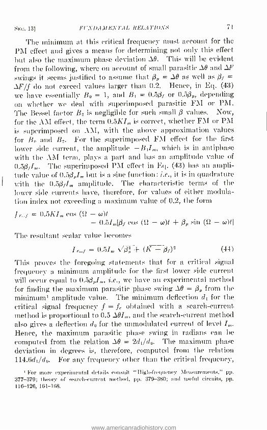
Six. 13] FI'.\' DAM E'NTAL BELAT IONS î 1
The minimum at this critical frequency must account for the PAI effect and gives a means for determining not only this effect but also the maximum phase deviation O. This will be evident from the following, where on account of small parasitic AO and OF
swings it seems justified to assume that ßp = 09 as well as Of = OF /f do not exceed values larger than 0.2. Hence, in Eq. (43)
we have essentially Bo = 1, and B, = 0.513f or 0.50p, depending on whether we deal with superimposed parasitic FAI or PM. The Bessel factor B2 is negligible for such small ß values. Now, for the AM effect, the term 0.5K/, is correct, whether FM or PM is superimposed on AM, with the above approximation values for B and B2. For the superimposed FBI effect for the first lower side current, the amplitude -B11, , which is in antiphase with the AM term, plays a part and lias an amplitude value of 0.50,I,,,. The superimposed PM effect in Eq. (43) has an ampli- tude value of 0.5/3,I,,, but is a sine function : i.e., it is in quadrature with the 0.50f1,,, amplitude. The characteristic terms of the lower side currents have, therefore, for values of either modula - tion index not exceeding a maximum value of 0.2, the form
= 0.5K1,,, cos (12 - co)t
- 0.5I ,[ßf cos (St - co)/ + ßp sin (SI - co)/1
The resultant scalar value becomes
= 0.51, Jßß + (K - ßf)22 (44)
This proves the foregoing statements that for a critical signal frequency a minimum amplitude for the first lower side current will occur equal to 0.50,,I,,,, i.e., we have an experimental method for finding the maximum parasitic phase swing AO = ßp from the minimum' amplitude value. The minimum deflection d, for the critical signal frequency f = obtained with a search -current method is proportional to 0.5 SOI, , and the search- current method also gives a deflection do for the unmodulated current of level Im.
Hence, the maximum parasitic phase swing in radians can be computed from the relation AO = 2d1/ do. The maximum phase deviation in degrees is, therefore, computed from the relation 114.6d, /do. For any frequency other than the critical frequency,
' For more experimental details consult "High -frequency \leasurements,'' pp 377 -379; theory of search- current method, pp. 379 -380; and useful circuits, pp. 116 -126, 164 -168.
www.americanradiohistory.com

72 FREQUENCY MODULATION [CHAP. I
the di deflections, as well as the d2 deflections shown in Fig. 21 for the upper first side current for different signal frequencies f, are larger. It is easy, therefore, to find out experimentally whether we are obtaining deflections for the lower side current or for the upper side current.
From this figure we see that, for a known degree K of AM, we can also compute the maximum parasitic frequency deviation F. Expressing the deflection readings in per cent, the deflection do = 1.0 corresponds to 100 per cent, and all other deflections are as indicated in the figure. Since at the critical frequency fe = 1.5 kc, we find the minimum value di = 0.08 and the dip of the
d =do 1.0-
0.5K-áFJdo
0.8
o
a`> 0.6 "ci= co
d,-def/ection i
0.4
f = fc is critical signa/ frequency of /.5kc for K =0.2
; c12-deflections
K=0.2
Minimum F
deflection F-f 4 -
d1= 0.508da FIG. 21.- Experimental di and d2 curves for the determination of OF if K is known and
K if ß = iF /f is known.
experimental di curve is 0.12 below the K level, we have 0.5 M = 0.C8 and 0.5(K - OF /fe)do = 0.5(0.2 - OF /1.5) = 0.12. Hence, 0B = 0.16 radian or ± 9.17 deg and OF = ± 0.06 kc or ± 60 cycles per second. To plot the deflections on a percentage scale has, furthermore, the advantage of showing with the di and d2 curves directly the effective Ke or modulation characteristics when all three types of modulations act simultaneously. Since both deflection or Ke curves run asymptotically toward the K line, which is due to AM and constant for all signal frequencies, we note that for higher signal frequencies neither parasitic FM nor PM can be very effective for the upper a -f range of signal currents in comparison with the desired AM. Whatever effect is still existent must, be mostly due to parasitic PM since AF /f is then very small in comparison to M.
www.americanradiohistory.com

SEC. 13] FUNDAMENTAL RELATIONS 73
It should be clearly understood that this experimental method puts no limit on the degree K of AM, but neither OF% f nor DO
should ever exceed values larger than about 0.2. This limitation seems amply justified if AM is the desired type of modulation. Even though the relations leading to this experimental method were obtained only from a comparison of FM + AM and PM + AM in Eq. (43) and not directly from FM + PM + AM as given in Eq. (42), it should not matter since we are interested only in
amplitude effects. As a matter of fact, if we would write down
the expression for pure AM as in Eq. (3), then write down the expression for pure FM as given by the
Ji(ß)I,n[sin (S2 + w)t - sin (S2 - w)t]
term of Eq. (12), but for the value J1(ß) = 0.50f which is per- missible for 0 values smaller than 0.2, and then write down also the expression for PM, the same formulas would be obtained.1
If we expand Eq. (42) into component terms, just as was done in Eq. (25) for PM + AM, using values of 0 that never exceed 0.2,
then the first Bessel factor B1 = 0.50, which value holds then for ß = 0, as well as for 0 = ßf. Now if we put Bo = 1 and B2 = 0,
which is permissible for ß < 0.2, we have, for the lower and upper first side currents, which are essentially the only side currents that can play a practical part for such a small modulation index 0,
for FM + PM + AM the expressions
0.5KIm cos (S2 - w)t - 0.5I ,[0f cos (S2 - w)t + 13 sin (9 - w)t] for F -f
(45) 0.5KIm cos (11 + w)t
+ 0.5Im[0f cos (S2 + w)t + ßP sin (S2 + w)11 for F f
which leads to the experimental method already found. If only the approximation B1 = 0.50 is used, retaining the true Bessel
factor Bo instead of the approximation Bo = 1 and also retaining the small Bessel factor B2 instead of neglecting it, we find for the first lower side current the scalar or amplitude value
I
IF -f = 0.5Im \/(Bo + B2)2[ß + (K - ßf)2] - 4BoB2 ßPK2 (46) ßP ßr
The last term under the radical surely cannot play a great part since, on account of the factor 0r in the numerator, even if 0P = 0.2,
we have a multiplier of only 0.04. In addition, even if either 0
This has been done in "High- frequency Measurements, p. 380.
www.americanradiohistory.com

74 FREQUENCY MODULATION [CHAP. I
value is as large as 0.2 we have B2 equal to only 0.00498. Hence, even for the upper limit where our deflection method still gives reliable results for OF and M, the portion 4B0, which is essentially equal to 4, of the last term under the radical has to be multiplied by a value 0.005 X 0.04K2/0.08 = 0.0025K2. For the most severe condition of 100 per cent AM, this factor is as small as 0.0025. We have, therefore, for the first side current the absolute amplitude
( IF±f = 0.5(B0 - B2)/in 002 + \K ±
z )
Since, for p = 0.5(Bo + B2)Im, we have
l (47)
r z IF±f = p26,02 + p21 / K
the current vectors for the respective first side currents are as in Fig. 22. From the resultant vectors it will be noted not only that
p= 0.5[Jo(ßJ*J2(ß)]Im 0.5 fm for critiar /frequency f
45°
p fF.actsdownward
pK acts upward
pK
F -f F f F F+F FIG. 22.- Resultant side currents for frequencies F f of first side current pair.
different projection (vertical) amplitudes result, but also that decidedly different directions prevail. It should be understood that the upper side -current vector spins around faster than does the lower side -current vector but that, in measuring side -current amplitudes, only the projection along the vertical coordinate is of interest. Hence, the PM effect on the lower side -current side must, for the critical frequency f = fc, which produces the mini- mum deflection dl, be equal to the magnitude p M since the second term in Eq. (47) vanishes for this frequency. For partial cancellation of the AM by FM effect, the dotted vector triangle
www.americanradiohistory.com

SEC. 14] FUNDAMENTAL RELATIONS 75
shows that the projection of the resultant amplitude on the verti- cal reference axis no longer gives p AO since the vertical and the horizontal portions of the dotted rectangular triangle are no longer equal.
14. Translation of Signal Currents into Corresponding Fre- quency and Phase Variations. -In Fig. 2, the stimuli that bring about FM and PM, respectively, are either frequency variations for direct FM or variations in phase for PM. Unless sound waves are used directly to bring about FM, we have to deal with either a signal or modulating current or its corresponding voltage. To use sound waves directly to produce FM has reference, for instance, to the use of a condenser microphone, which acts as a part of the circuit capacitance, the capacitance determining partly the frequency F of the carrier current. With such a system, though straightforward, we could not produce modern wide -hand FM nor expect to secure good mean carrier -frequency stability. Hence, the problem is to translate a signal- current variation into cor- responding frequency swings about the mean carrier frequency F in the case of FM, or into such equivalent corresponding frequency swings [Eq. (6)] about the fixed' carrier frequency F in the case of PM. The latter is primarily done by having the signal current cause corresponding relative phase variations in the carrier, while the unmodulated carrier level Im and the carrier frequency F are kept constant.
Even though, with FM as well as with PM, the value of the center frequency F remains constant as far as the number of cycles per second is concerned, there are, according to Eqs. (7) and (6), great differences. For FM the corresponding frequency variation is directly proportional to the maximum frequency excursion OF during the modulation cycle [Eq. (7)]. For PM the equivalent frequency variation is likewise proportional to the maximum excursion, which is in this case, of course, a phase swing 0O, but it is in addition also directly proportional to the frequency f of the signal current [Eq. (6)].
We have also to take into consideration the time function cos wt affecting the instantaneous magnitudes of the FM as well as of the equivalent FM swings. Generally, if PM acts with all
' It should be clearly understood that for PM as well as for indirect FM, the primary oscillator can be a stabilized piezo oscillator since the carrier frequency F is fixed and we have frequency variations only in equivalence.
www.americanradiohistory.com

76 FREQUENCY MODULATION [CHAP. I
the features of true phase modulation, a sinusoidal current im sin cut
causes in Eq. (5) the AO sin wt variation. This could be brought about by means of a corresponding signal voltage impressed on respective screen grids of a balanced modulator (consult Fig. 52). The amplitude of the signal voltage is in this case em, corresponding to im of the signal current. The screen grids are driven in push - pull, but the control grids of the two tubes of the balanced modula- tor are connected together. A carrier voltage of fixed frequency F is applied between the parallel control grids and the respective cathodes, which are likewise connected together. Therefore, the carrier voltage acts in equal pull. The push -pull output on the plate side can yield only the modulation product (Kim sin wt) sin Sgt
since this is a modulator in which the unmodulated carrier is automatically suppressed. These products exist, therefore, only at instants when the signal voltage has a value. Hence, the modulation product is proportional to the signal -voltage variation.
If, as in Fig. 3b, this modulation product, which is an AM product, is added in time quadrature, as far as the period 1/F of the carrier current is concerned, with the unmodulated carrier, we shall have PM with a phase variation AO sin wt, which is proportional to the signal current. This phase shift takes place in the external plate circuit as shown in Figs. 52, 72 and described in detail in connection with them. Hence, the condition required in Eq. (5) can be readily satisfied; i.e., a signal -current variation is readily translated into proportional phase swing modulation which is PM.
But from Eq. (6) we note that the equivalent frequency varia- tion superimposed on the fixed carrier frequency F is by no means the same as the signal- current variation as far as the entire a -f range is concerned. We note that the degree of equivalent FM becomes larger for the higher signal frequencies f than for the sounds of lower pitch. For equivalent FM, we have inherent a -f emphasis, i.e., frequency accentuation toward the upper signal - frequency range. This is characteristic with PM and does not mean distortion, since the actual PM effects are still directly proportional to signal- current variations. Hence, if in a receiver we use a phase discriminator instead of a frequency discriminator, PM would be demodulated properly and without such a -f accen- tuation. But when we are interested in producing equivalent FM variations with no accentuation of this type and as with FM
www.americanradiohistory.com

SEC. 14] FUNDAMENTAL RELATIONS 77
[Eq. (7)], then we can do this only if we cause at the output of the balanced modulator a modulation product which is not only of
the general form (KI, sin wt) sin Sgt but which has an amplitude
KI ", 5111 wt f
instead of the amplitude KI, sin wt. When such a modulation product, namely, (KIm/ f) sin wt sin Sgt, is added in time quadrature, i.e., as (KIm /f) sin wt cos Qt, with the unmodulated carrier I, sin Sgt, we cause in Eq. (5) not maximum AO excursions but max-
imum z O/ f excursions. The equivalent change in instantaneous frequency in Eq. (6) is no longer f AO cos wt but is M cos wt.
Hence, the equivalent FM is exactly the same as though direct FM had been the cause. A frequency discriminator will, so to
speak, not "feel" whether the cause of its FM into AM conversion was due to direct FM or indirect FM. This is exactly what is
done in the well -known Armstrong transmitter. The only "link" still missing is how the 1/f effect is injected
into the balanced amplitude modulator. This task is simple also.
Since Eq. (6) was obtained by differentiation of the argument a of the main sinus function sin a of Eq. (5) in order to account for the instantaneous frequency Ft, and since in the representations of Fig. 7 equivalent PM is an integration of FM, we must integrate the signal current before applying the corresponding voltage to the balanced modulator. Integrating, for instance, i, cos (6.28f)t
yields [m sin (6.28f)t A]/(6.28f); i.e., a similar function of time whose amplitude is also inversely proportional to the signal
frequency f. The integration constant A is here of no practical concern. Electrically, such an integration takes place in any con-
denser since its terminal voltage is proportional to f (in cos wt) dt,
the constant of proportionality being the reciprocal of the capaci- tance, i.e., equal to 1 /C. All that is necessary, therefore, is to apply the actual signal voltage to a series combination of a high
resistance and a condenser. Then have the voltage of the con-
denser affect the balanced modulator. This is usually done through an amplifier tube on whose fixed grid -cathode bias is
superimposed the integrated voltage that is now proportional to e, /f, since 1/C as well as 1/6.28 are constants. This is described in detail on pages 223 to 225. It is, therefore, seen that we can pro- duce true FM effects even though PM is primarily instrumental if
www.americanradiohistory.com

78 FREQUENCY MODULATION [CHAP. 1
the complex signal current due to any signal or intelligence is made to flow through the resistance- condenser combination.
The signal current translation into a similar variation of the carrier frequency F in direct FM presents no engineering difficulty either. As a matter of fact, very large frequency swings can be secured directly since in practice a variable reactance is reflected into the oscillator branch that determines the carrier frequency F. This is done by a superimposed current which is fed back into that branch and which can, therefore, cause frequency variations that are directly proportional to the signal current. (For details, consult pages 155 to 182.) From this it is again evident why for direct FM the primary oscillator cannot be a piezo oscillator whose frequency is inherently stabilized.
15. Translation of Frequency Modulation and Phase Modula- tion into Amplitude Modulation. -Since both FM and PM are time axis modulations that are in quadrature with modulations in amplitude, customary types of demodulators cannot be used for separating the signal component, i.e., the intelligence, from the modulated carrier current.
In the first detector and the i -f networks of an FM receiver, everything is the same as for customary types of superheterodyne circuits used in AM receivers. However the band -pass networks have to accommodate a frequency spectrum corresponding to the maximum deviation ratio AF /fig = 5, where ff is the highest ,desired signal frequency and is generally taken as 15 kc. With respect to the second detector, this must do the same thing, but in the other direction from that which brought about the frequency modulation in the transmitter. As far as PM is concerned, even though a variable phase swing causes PM, we have learned that it causes also equivalent frequency swings with an amplitude value f M. Therefore, we can consider a PM current as one for which the equivalent frequency swing is proportional to the signal frequency as well as to the signal amplitude. This can be taken care of by means of a frequency -correcting network, which con- nects to the output of a discriminator.
Equation (10) shows that an FM current has the form
It = I, sin (S2t -l- ß sin wt) = Im sin S (48)
in which ß = AF /f for FM and ß = M for PM. This expression represents the results of FM or PM and it is the action that has to
www.americanradiohistory.com

SEC. 15] FUNDAMENTAL RELATIONS 79
be reversed in the second detector of a receiver. All that interests
us in this expression is the main sine function which is the argument
6 since it, and not the amplitude Im, which for pure FM as well as
pure PM must remain constant, controls the modulation energy.
Any amplitude variation must be in quadrature with the FM
and will require a different means of detection. In case of FM
the argument S is the outcome of an integration since for FM,
according to Fig. 2, we start with an instantaneous frequency
F1 = F + OF cos wt which multiplied by 6.28 yields the cor-
responding instantaneous angular velocity Qt. In order to obtain
the instantaneous phase angle of the modulated current, we
integrated SZt and found f (S2 + OSZ cos wt) dt = Sgt + (M2/co) sin wt,
if the integration constant is ignored. This constant represents
a fixed relative phase, which can contribute nothing to the
modulation. The outcome is the S value in Eq. (48).
This means, in other words, that our demodulator in the FM
receiver must differentiate in order to reverse the integration action
in the transmitter. Performing this differentiation, we have
d6/dt = SZ + coß cos wt which yields exactly the original function
SZ + ASZ cos wt that caused FM in the transmitter. Hence, the
demodulation of direct FM with a time rate detector should not
cause distortion as long as the demodulator has a linear range for
the entire peak -to -peak frequency swing of, say, 150 kc if AF =
+ 75 kc. We still have PM and indirect FM to consider, the
latter being used in the Armstrong transmitter. With respect to Fig. 3b, we learned that PM can also be
produced by adding the modulation product (KI, sin wt) sin SZt,
as obtained at the output side of a balanced amplitude modulator,
to the unmodulated current vector Im sin Sgt and in time quad -
rature with it. Hence, the modulation product is added as
(KI, sin wt) cos SZt, which is now a cosine function of the carrier cur-
rent variation. The geometrical addition shown in Fig. 3b indicates
that the resultant vector OP1 is longer than I, and has a magnitude
-0P2 + PPi = Im V/1 + K2 sin2 wt. It makes, at any instant, an angle et = tan-1 (PP1 /OP) = tan-1 (K sin wt) with the vector
OP which represents the Im sin Sgt variation of the unmodulated carrier of frequency F.
If we can express the resultant vector OP1 at any instant in the
form of Eq. (48), we know from the proof given above that a linear
differentiator, or, as it is called, a frequency discriminator, will
www.americanradiohistory.com

80 FREQUENCY MODULATION [ Crine. I
demodulate the modulation intelligence. Since this PM is caused primarily by AM, we have to express K in terms of equivalent phase effects. Writing down the expression for the instantaneous value of the resultant vector 0P1j we find
It = Im + K2 sin' wt sin (S2t + et)
= Im A/1 + K2 sine wt sin (S2t + sin wt) (49)
where for all values of primary AM, i.e., K s 1, a corresponding maximum phase swing 43 obtains. From the expression Ot = tan-1 (PP1 /OP) = tan-' (K sin wt), we note that for in degrees we have tan = K. Now, let us examine the most severe primary amplitude modulation condition for which condition K = 1. Figure 3b, as well as the corresponding equations, shows that then PP1 = OP and 43 = 45 deg. This is the maximum phase swing that can be produced with a balanced modulator ahead of this PM device. This assumes that the Im sin Sgt vector, which is sup- pressed in the balanced amplitude modulator, is added in quad- rature and is not a vector that is shorter or longer than Im but is equal to it. Since in Eq. (48), which we have to satisfy for no distortion, the maximum phase swing ß = AO is in radians, we have to obtain also in radians. For the 100 per cent primary AM assumed above, this gives cic. = 45/57.3 = 0.758 radian. Hence, we cannot equate 43 radians to the AM factor K, which .
causes 43 and is K = 1. Therefore, for phase swings as large as 45 deg, the resultant vector OP1 will not travel with its extremity on a circle. Therefore, considerable harmonic distortion will take place.
Now consider the case where only 20 per cent AM is effective in the balanced modulator that produces the modulation product KI, sin wt sin Sgt before it is shifted 90 deg with respect to the carrier angular velocity S2. We then have K = 0.2 and find cf. = tan' (0.2) = 11.3 deg or 11.3/57.3 = 0.1974 radian, which is essentially equal to 0.2 = K. Looking at trigonometric tables, we find that K = 0.2 is about the upper limit producing phase swing linearity at any instant of the modulation cycle of the 0.21m sin wt variation. This is true since for the most severe condition of the modulation cycle the value K = it /Im = 0.2 causes a tangent essentially equal to the angle in radians. Hence, we have
www.americanradiohistory.com

SEC. 15] F TNDAME.tiTAL RELATIONS 81
It = Im V 1 + K2 sine wt sin (S2t + K sin wt) for K <_ 0.2 and K = B (50)
and exactly the same expression as in Eq. (48) is obtained. Equa- tions (49) and (50) show that AM also takes place, but is negligible for K < 0.2. Otherwise it has to be avoided by clipping off the amplitude variations by means of an amplitude limiter. This will, however, take some of the modulation energy away and will cause a certain amount of distortion as can be seen from page 59. Hence, pure PM as expressed in Eq. (50) can be readily demodu- lated with a frequency discriminator. But it has to be realized that a frequency -correcting network has to follow in order to make up for the a -f emphasis toward the higher a -f range on account of the f term in Eq. (6).
Now the next step is to find out how indirect FM can be demod- ulated. At first sight it looks as if, since indirect FM has all the features of direct FM, Eq. (48) holds and indicates that a linear frequency discriminator will demodulate this type of modulation without harmonic distortion. It will be remembered, however, that indirect FM is initiated by an amplitude modulation product in quadrature with the unmodulated carrier as in Fig. 3b. The only difference that exists is that Armstrong uses a 1/f network based on integration (consult page 77), of the signal current between the signal- frequency source and the balanced amplitude modulator. Hence, a signal voltage of amplitude em; f is impressed in push -pull on the screen grids of the two modulator tubes. This means that the modulation product taken off at the output side of the balanced modulator is now proportional to
(Kt' sin cot) sin Slt = p sin S2t
amplitude
When this product is shifted by 90 time degrees and combined with the unmodulated carrier, there results an instantaneous current value
Ic=I, sill S2t p cos Slt=
where
K2 1 + f2 sine wt sin (SU + 0t) (51)
0 tali ' (-f sin wt) (51a)
www.americanradiohistory.com

82 FREQUENCY MODULATION [CHAP. I
Matters are much more favorable in this case than for PM without 1/f correction. We see, for instance, that the undesired AM has now only a KI,n /f extreme component amplitude swing instead of Kim; i.e., it becomes smaller as the signal frequency f is raised. As far as the resultant amplitude variation that is actually effective is concerned, we find even for 100 per cent primary AM an extreme resultant amplitude of only In, 1 + m where m = f -2. Hence, even for the lowest audible frequency of f = 16 cycles per second, we have essentially unity for the square -root value. This assumes that the proportionality con- stant that causes the 1/f effect is unity. The other favorable factor is the fact that the maximum phase amplitude 4 in 9t = 4 sin wt now depends on K/f instead of on K. We have for such a substitution the expression
K2 It = I, 1 + sine wt sin (S2t + 41 sin wt)
tan 4/ = f (52)
Hence, the largest maximum phase excursion takes place at the lowest signal frequency f; this is important. In the Armstrong system a maximum phase swing of ± 30 deg is not exceeded. But, according to the foregoing numerical speculations, if also here >li < 11.3 deg then we can use AO instead of 4' which corresponds to a maximum of 0.2 radian. Consequently, for angles even as low as ± 30 -deg maximum phase excursions, a certain amount of distortion will take place, as was already discussed on page 6. To find out the order of this distortion, we need only consider the argument of the main sine function sin (pt + 4' sin wt). Since generally the constant of proportionality for the 1/f correc- tion, as well as the gain of the modulation network, will not result in unity values, we have to replace K by k = qK, where q takes. care of the resultant constant of proportionality. Then we have tan 41 = k/f and for the sine function the argument y = SZt + tan-' (k /f sin wt) which for k, f = p leads to the demodulation solution which must be the time rate of change of y, or
dy S2
Pf cos wt - k cos wt ky (53)
dt 1 + p2 sine wt 1 + p2 sine wt
www.americanradiohistory.com

SEC. 15] FUNDAMENTAL RELATIONS 83
where p denotes the maximum phase swing. We note that only amplitude distortion prevails. Hence, the term u = cos wt /(1 + p2 sine wt) represents the magnitude of the distortion.
It is, therefore, seen that for direct FI\1 and for indirect FM, which does not produce maximum phase swings much larger than about 11.3 deg, a linear time -rate demodulator can, as is shown in Fig. 23, translate without distortion frequency variations into corresponding amplitude variations. A linear time -rate demodu-
Output vo tage
w=2aP 2E -T
I
E 4-1---t- E, I
]F1--
Ft
r.
,Input frequency variations
Output vo tage
Output l amp /itude variation
Time
Fm. 23.- Conversion of frequency variations into amplitude variations.
lator is a device that gives output voltages that are directly propor- tional to frequency variations. The frequency variations are about the center frequency F and the 2 AF demodulator accom- modates a complete peak -to -peak frequency swing. Since the output of any modulation device is always some function of the amplitude, one or even two amplitude limiter stages should be used ahead of the FM -AM translator. This ensures that relatively large undesired amplitude variations do not remain in the output of the last limiter where they can affect the frequency amplitude converter.
www.americanradiohistory.com

S4 FREQUENCY 11l()l)(7.:1 TlO.v !CHAP. I
The converter, or frequency discriminator, shown in Fig. 23,
is assumed to have an ideal characteristic in order to bring out clearly the modulation conversion. The characteristic is such that for the upper cutoff frequency F,, of the slope filter a voltage 2E is obtained at the output of this filter. For the center or carrier frequency F we have only a voltage of E volts; at the lower cutoff frequency F1 zero output voltage prevails. The charac- teristic also covers a maximum range or frequency width of
1V = 2 OF = 150 kc in order to meet current practice. Hence, if the input voltage has frequency swings over the limits of ± 75 kc, the total width 11" for which the slope converter is designed will be made use of and maximum permissible frequency excursions will
be converted into 100 per cent AM at the output of the modulation converter. If, however, not so intense an FM is arriving at the input side of the modulation converter then, as is indicated in this figure, we shall cover a total frequency space or width of only 1V1
for corresponding frequency fluctuations of +ZVI. The degree of amplitude modulation experienced at the output side of the FM -AM' translator is then no longer 100 per cent but is K = 200 AF1j 1V1 per cent.
The ideal characteristic has the disadvantage that it taxes the receiver even at times when no FM exists, since for absence of FM the output voltage is not zero but = E volts. This characteristic has the disadvantage that it is not symmetrical, at the center frequency F, with respect to a differential action due to output voltages on each side of this frequency. To eliminate these disadvantages, commercial frequency discriminators are designed such that at the center frequency F there is no output voltage at all. For a certain positive OF1 swing we obtain, say, a certain positive output voltage proportional to the magnitude AF1 of this swing; for the same negative swing -AF1, we obtain an equal negative output voltage from the discriminator. Such an action is brought about by push -pull modulation translation. Since such discriminators use rectifiers, they will inherently also bring about subsequent amplitude demodulation so that signal frequency output occurs. Li such discriminators a certain positive frequency deviation AF1 from the center frequency F causes an increase of the output voltage of one tube section; at the same time, a decrease occurs at the output of the other tube section (two rectifers under one envelope). As far as the input
www.americanradiohistory.com

SEC. 16] FUNDAMENTAL RELATIONS 85
side of the two sections is concerned, they behave exactly alike. This explains the differential action at the output side and shows
that we have not only frequency discrimination but also an apparatus from which, for equal simultaneous positive voltages of frequencies F OF1 and F - OF1, there can be no output voltage. This feature will eliminate certain types of static inter- ference. To accomplish such differential action, the output branches of the rectifier units are connected in indirect series.
The respective output voltages therefore add and cause a double amplitude effect; in absence of FM, no output effects exist.
The elimination of certain types of static is based on the fact that when certain abrupt interference (consult Fig. 31) arrives at the i -f stages of the FM receiver, it produces, in virtue of the band -pass action of such a network, a series of spectrum ampli- tudes of the same polarity acting simultaneously and symmetrically with respect to the mid -frequency of the band -pass network. Hence, such disturbances can only enter the discriminator, but cannot produce any output voltage that will act on the a -f stages of the FM receiver. It should be understood, however, that if a
relatively significant FM at the same mid -frequency also occurs, the instantaneous relative phase of the interfering spectrum energy distribution with respect to the FM carrier may have any value whatsoever. This is explained on page 104 and shows that if the phase of the interference is, for instance, 90 deg leading the FM current of mid -frequency F and if the interference intensity I is larger than the desired FM intensity D, then the instantaneous phase of the resultant of I and D is also varied, owing to the I action. This equivalent PM caused by the interference will
affect the output voltage of the discriminator and will, therefore, also register some of the interference at the a-f output of the FM receiver. This is not true, however, when I is much smaller than D, as the explanation in connection with Fig. 29 shows.
16. Determination of Maximum Frequency and Maximum Phase Deviation and of the Mean Carrier Frequency.- Experi- mental methods of determining maximum frequency and maximum phase deviations are required in order to assure, for instance, that the maximum permissible frequency swing of ±75 kc is not exceeded. Otherwise a wider frequency spectrum than permissible might be produced, which might even exceed the width of the guard band between adjacent frequency channels and cause
www.americanradiohistory.com

86 FREQUENCY MODULATION [CHAP. I
interchannel interference. The Crosby method of determining maximum frequency deviations consists in determining the condi- tions for which the Bessel curve of zeroth order,' the Jo(ß) curve, intersects the ß axis; i.e., where the Bessel factor governing the amplitude of the carrier frequency F becomes zero. This occurs,
100,.
0.8 -Jo (fi)-Mu//io/i& ofcurrenf of frequency F
0.6
04 Jo(ß)
0.2
0.2
24048 - 8.6537 _/4.9309 5.5201 - 1179/5 /8.071/
--A 21.2//6; 274935;30.6346;337758: 04 40.0584;431998;4624/2 ; 49.4826
52.624/; 55.7655 ;58.9070; 62.0485 etc.
Sound intensity in superheterodyne AM receiver
s i \\ / \ , -.
1 i i .' \ , - - -.\ , -- 11 1/ 1I 1I I / ii ii 8 8 8 d h
fF
FIG. 24.- Experimental determination of the maximum frequency deviation OF'.
according to Fig. 24, for the first point of intersection for a ß value of 2.4048, for the second intersection for ß = 5.5201, etc. Since ß = .F /f and the signal frequency f is known, we can compute the maximum frequency excursion OF, which causes zero amplitude effect for the carrier frequency F when the OF swing is sufficient to produce such values as are given in this figure. The method consists, therefore, in determining the disappearance of the current amplitude of carrier frequency F when a suitable FM exists either by varying the signal frequency f, if the order of this frequency is of no concern, or by varying the value of IF.
1 Any Bessel curve, such as the J,(ß) or the J,(ß) curve, could be used with the respective a-axis intersections. But on account of other zero spectrum amplitude effects (consult p. 41), it is best to use the J0(ß) curve.
www.americanradiohistory.com

Sic. 16] FUNDAMENTAL RELATIONS 87
Any of the search -current methods' can be used although an ordinary superheterodyne receiver of the type customary for amplitude modulation will do. The first step is to tune the superheterodyne receiver to the carrier frequency F of an unmodu- lated FM transmitter. The i -f selectivity should be as narrow as possible. The oscillator frequency of the superheterodyne is so
chosen that a low beat sound, say a 100 -cycle note, is heard in a headset. Suppose a 4 -kc signal (f = 4,000 cycles per second) is
gradually applied to the modulator of the FM transmitter by raising the signal voltage e,,, cos wt from zero level on upward. As the voltage is raised, the degree of FM is also increased and, therefore, also the value AF in ß, because f = 4 kc is fixed. Hence, ß will also increase with the signal voltage applied to the modulator and will cause more and more side currents. As the frequency spectrum spreads, the modulation energy moves more into the side bands and, according to Fig. 24, the amplitude I,,,J0(ß) of
carrier frequency F decreases until for a ß value of 2.4048 the carrier frequency amplitude must vanish altogether. Hence, by increasing the applied signal frequency voltage from zero volts upward, we gradually decrease also the intensity of the beat note of 100 cycles per second heard in the headset of the AM receiver until essentially zero sound effect is noted for the ß = 2.4048 condition. Hence, at this point we have
AF = 2.4048 X 4 = 9.6192 ke
which is altogether too small a frequency excursion for modern wide -band FM work. A further increase of the signal voltage applied to the modulator again raises gradually the intensity of the 100 cycles per second note toward a certain maximum sound sensation. Then the intensity decreases again gradually until for ß = 5.5201 essentially silence again occurs. This gives the maximum frequency swing OF = 5.5201 X 4 = 22.08 kc. If the signal frequency had been 15 kc for this condition, then the maximum frequency swing would have been 5.5201 X 15 = 82.8 kc.
Hence, if a suitable voltmeter is connected across the input terminals of the modulator as such measurements are being made, the readings on it can be expressed in terms of corresponding frequency swings. Since for the determination of large OF swings,
Consult footnote, p. 71.
www.americanradiohistory.com
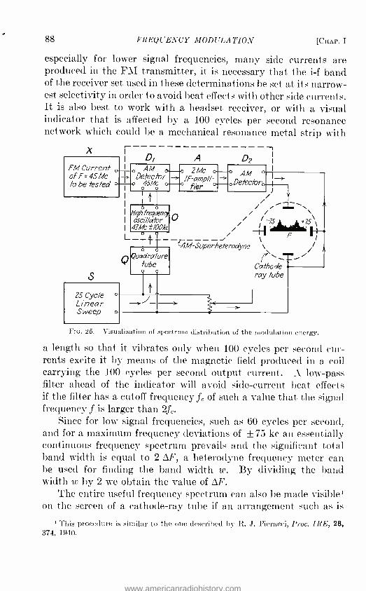
88 FREQUENCY MODULATION [CHAP. I
especially for lower signal frequencies, many side currents are produced in the FM transmitter, it is necessary that the i -f band of the receiver set used in these determinations be set at its narrow- est selectivity in order to avoid beat effects with other side currents. It is also best to work with a headset receiver, or with a visual indicator that is affected by a 100 cycles per second resonance network which could be a mechanical resonance metal strip with
X I D,
FM Current . off= 45 Mc
1-0 Detector
isbe tested
S
25 Cycle o
Linear Sweep o
T
41 frequen oscillator
43Mc ±í00k O //
.j ,,-?75,,\\,, // 7
F I
ÁM-Superheterodyne
A D2
2Mc o o ,4M o
IF-amp/io- .Detector. j- fier
Cathode ray tube
FIG. 25.- Visualization of spectrum distribution of the modulation energy.
a length so that it vibrates only when 100 cycles per second cur- rents excite it by means of the magnetic field produced in a coil carrying the 100 cycles per second output current. A low -pass filter ahead of the indicator will avoid side -current beat effects if the filter has a cutoff frequency f, of such a value that the signal frequency f is larger than 2fr.
Since for low signal frequencies, such as 60 cycles per second, and for a maximum frequency deviations of ±75 kc an essentially continuous frequency spectrum prevails and the significant total band width is equal to 2 OF, a heterodyne frequency meter can be used for finding the band width w. By dividing the band width w by 2 we obtain the value of F.
The entire useful frequency spectrum can also be made visible' on the screen of a cathode -ray tube if an arrangement such as is
'This procedure is similar to the one described by R. J. Pieracci, Proc. IRE, 28, 374, 1940.
www.americanradiohistory.com

SEC. 161 FUNDAMENTAL RELATIONS 89
shown in Fig. 25 is employed. In this figure X denotes the FM source to be tested with respect to the frequency spread and maxi-
mum frequency excursions; 0, Di, A, and D2 are sections of a
superheterodyne unit. In this illustration the frequency of the test current is taken as 45 Mc while the i -f amplifier A works with a center frequency of 2 Mc. Hence, the oscillator frequency of 0 is set to a center frequency of 43 Mc. It will be noted that the oscillator 0, which causes the beat effect to initiate a carrier of
center frequency of 2 Mc by superposition of the test current coming from X and the oscillator current in the first detector D,, is also frequency modulated with maximum frequency deviations of ± 100 kc, which are larger than the frequency deviations that will ever occur in the test current. The FM in the oscillator 0 is
caused by a quadrature tube modulator Q, which is also known as a
reactance tube (for details see Secs.. 29, 30). This quadrature tube Q is driven by a linear sweep voltage coming from the output of a saw -tooth oscillator S. The same sweep voltage also acts directly on one deflection condenser of the cathode -ray tube. The linear sweep scans, therefore, the center frequency of 43 Mc
of the local oscillator 0, 100 kc below and 100 kc above the center frequency of 43,000 kc. Hence, it must also register at the amplifier A any other signals that it meets during such frequency swings, as long as the signals do not fall outside the peak -to -peak swing of 200 kc. Owing to the beat action between the 43 -Mc oscillator current and the test current of center frequency of 45 Mc,
we have decreased the center frequency of 45 Mc to a new center frequency of 2 Mc as far as the center frequency of both sources
X and 0 are concerned. However, the center frequency of 43 Mc
experiences linear off swings toward 42.9 and 43.1 Mc and, there- fore, currents of such an instantaneous local oscillator frequency can cause beat effects with any of the side currents of source X due to any OF swing of the test current, provided the magnitude of this swing does not exceed ± 100 kc. The result is that in the mixer D1
we have at its output just as many side components as are in the original test current, i.e., in the FM current to be examined. The only difference is that these side components are with reference to a center frequency of 2 Mc instead of 45 Mc. The succeeding amplifier A will enlarge the effects of these components, and the detector D2 will separate the positive swings of the spectrum components. The output of D2 applies, therefore, to the other
www.americanradiohistory.com

90 FREQUENCY MODULATION j('nnr. I
deflection condenser of the cathode -ray tube spectrum pulses, which resemble sharp resonance curves for each side current. Hence, when a large AF swing exists in the FM of the test current, the spectrum width noted on the screen of the cathode -ray tube must be equal to 2 OF for a low- signal frequency f of about 50 cycles per second. Suppose we had actually a OF modulation of ±75 kc, or at least very close to it, operative in the test FM cur- rent. Then all that, is necessary is to change the signal frequency f gradually to higher values toward a value in the neighborhood of 15 kc, since this would give a ß value of about 5, and then to note at what signal frequency f the center current amplitude vanishes. This must occur for a ß value of 5.5201. Since, according to Table III, we have only about eight significant side currents on each side of the center frequency for ß values in this neighborhood, i.e., close to 5, it will be an easy matter to recognize the center amplitude and to observe it vanish as the signal frequency f is varied around 15,000 cycles per second. Suppose the experiment shows that for f = 13.2 Ice the center amplitude disappears, then OF = 5.5201 X 13.2 = 72.9 kc. Hence, assuming that the OF condition is the same for the 50 cycles per second signal current modulation, then the width marked by the cathode -ray pattern gives the 72.9 -kc calibration. The band width caused by any other degree of F1 i in the current to be tested, with respect to OF swings, can he estimated from this calibration width.
On page 40 another method is shown for experimentally deter- mining OF, as well as 0O swings.
The mean carrier frequency F can be readily determined when the test current is not subjected to FM. This is done by beating the test current with a current coming from a source of stabilized and known frequency. If the test current is modulated in fre- quency, the unbalance in a frequency discriminator can be used for the determination of the mean frequency F. The discriminator output is fed into a low -pass filter with a cutoff at a very low frequency of about 25 to 30 cycles per second. The unbalance is measured with a microammeter. For the correct frequency value F there can be no deflection in this meter. (For details consult sections on discriminators.)
17. Effect of Band- restriction Filters on Currents Modulated in Frequency. -The required band width as indicated by the significant Bessel amplitudes can be narrowed only if it does not
www.americanradiohistory.com

SEC. 171 FUNDAMENTAL RELATIONS 91
cut off significant side currents. Suppose we are dealing with the frequency spectrum distribution shown in Fig. 8. This figure shows that for ß = 2 the significant terms have amplitudes proportional to the Bessel factors J7,(ß) = B , which are Bo = 0.2239, B1 = 0.5767, B2 = 0.3528, and B3 = 0.1289, giving for all practical purposes the solution
It = 0.22391, sin Stt + 0.5767I,7, sin (S2 + w)t - 0.57671ó sin (1-2 - w)t + 0.35281m sin (St + 2w)t + 0.35281ó sin (Sì - 2w)t + 0.1289/m sin (St + 3co)t
- 0.1289I7 sin (St - 3w)t (54)
for the FM current at any instant. We note that here we have three significant side currents on each side of the center frequency
PZ Limiter action
/ 95.
01'7= 1,7,1/02239'4(2x0.5767)2 P7 o
= 1/751,7,
PP = 05767ím =P,P2; OP= 022,791r,,
Fiu. 26.- Vector diagram for one side- current pair for distribution of 0 = 2 of Fig. 8.
2
í.1751m
F. Suppose we use a band -pass filter that passes only the first side- current pair besides the current 0.22391ó sin Sgt of carrier frequency. We have then the vector addition shown in Fig. 26 where vector OP represents the vector of the carrier frequency F with respect to position as well as amplitude value. The addition of the two side currents, which can also be passed by the filter, results in the quadrature vector PP2. The resultant instantaneous current vector is then OP2 which is longer than the amplitude or carrier level Im of the unmodulated current. A lengthening of the current vector can be produced only by a simultaneous AM, which did not exist in the spectrum solution (54) since it includes all the significant terms. Since both side currents move about P, we swing the phase of the resultant current emerg- ing from the band -pass filter over ±cl) degrees during the modu- lation cycle while the length of the resultant varies between the limits 0.22381ó and 1.1751,. Hence, we have an AM of 100 (1.175 - 0.2238) / (1.175 + 0.2238) = 68 per cent with twice the frequency of modulation. The resultant vector moves from OP2
www.americanradiohistory.com

92 FREQUENCY MODULATION [CRAP. I
with a maximum value of 1.1751m over a minimum value of 0.22391m to position OPz of maximum value of 1.175Iß and back over the minimum amplitude value to position OP2 of maximum value during the modulation cycle. When, therefore, the band -pass filter feeds into an amplitude limiter that saturates at amplitudes of 0.2239I,n, the AM produced by the band -pass filter is removed and the resultant vector flutters between the Opt and Op limits. Hence, all the even harmonic side currents are, so to speak, again injected by means of the limiter action. Since we have also odd harmonic side currents, they must account for the distortion that remains. From Eq. (54), as well as from the frequency spectrum of Fig. 8, we note that in this particular case the distortion of the only remaining odd harmonic is due to the amplitude 0.12891,n, which when geomet- rically taken into account shows that neglecting such a side - current pair causes a small distortion only.
18. Interference and Its Partial Elimination in FM Systems. - Generally, interference can be due to other FM stations on the same or adjacent channels. It can also be caused by AM stations as well by arriving carriers that are not modulated at all. Besides these, we have to deal with noise interference and random' dis- turbances, which occur in any high -gain amplifier.
Quite often distortions in FM receivers are not due to inter- ference at all but to poor circuit design in the receiver. Condi- tions in FM are in many respects vastly different from AM conditions. With FM the harmonic distortion does not depend principally on tube characteristics, as with AM, but more or less on the transmission characteristics of the transfer networks, such as the coupled tuned circuits in the i -f stages, the coupling to the discriminator, and the like. Fortunately, it is easier to design a linear transfer network than it is to design a linear tube such as would be needed for distortionless AM systems. In linear net- works for FM systems we cannot use designs that would be called free from nonlinear distortion when used in AM systems, since for AM a transfer characteristic that is symmetrical with respect to the carrier frequency F in amplitude as well as in phase is good engineering practice. In FM systems such a design would be satisfactory only for the lower signal- frequency range. Only in this range is the modulation index ß = OF /f fairly large if we
For details, consult "Phenomena in High -frequency Systems," pp. 255 -256 and "High -frequency Measurements," pp. 31 -32, 325.
www.americanradiohistory.com

SEC. 18] FUNDAMENTAL RELATIONS 93
assume maximum frequency deviations of about ± 75 kc, say, for signal frequencies below 100 cycles per second. Since we have to deal with the entire signal- frequency range, say up to 16 kc, and for different values of OF, i.e., maximum frequency excursions that are not necessarily so high as ± 75 kc because the frequency excursions may be the result of sounds of less than maximum loudness, we have to deal quite often with modulation indexes that cannot be called relatively large. Hence, all band -pass networks
must have transmission characteristics whose amplitude and whose phase are linear functions for all frequencies included in the band width. If only a symmetrical transfer characteristic were used, as for AM systems, nonlinearity of the phase characteristic would cause also nonlinear signal distortions. The effects of curvature in the amplitude characteristic could be avoided in many cases by the use of an amplitude limiter.
Generally, if two unmodulated carriers arrive in an FM receiver simultaneously and the difference of the respective carrier frequencies is relatively small compared with the magnitude of
each carrier frequency, then the superposition of both unmodulated waves in the mixer stage of the FM receiver causes not only beat effects that produce AM, but also effects that result in PM and, therefore, also equivalent FM. It is the equivalent FM that will
be translated by the discriminator into AM and then will be
heard as interference in the speaker of the receiver. The AM effect can be cut out by the amplitude limiters that precede the discriminator. According to Eq. (6), we have the term (F1 - F2) 09 cos [6.28(F1 - F2)t] for the equivalent FM, where F1
and F2 denote the respective carrier frequencies of the unmodulated currents that combine in the mixer stage. As it is assumed that the difference of these two frequencies is in the a -f range, we see
that a larger frequency difference causes more equivalent FM and, therefore, more interference, since the maximum equivalent frequency excursion is proportional not only to the maximum phase swing AO but also to F1 - F2. As we shall learn in Sec. 19
and as was already seen from the discussion on page 6, if the amplitude of one of the respective interfering unmodulated arriv- ing waves is twice the value of the other amplitude, then the quadrature addition causes a maximum phase deviation of AO = ±26.6 deg or ±0.4642 radian. Hence, a difference frequency of
50 cycles per second would produce an equivalent maximum
www.americanradiohistory.com

94 FREQUENCY MODULATION [CHAP. I
frequency swing of 50 X 0.4642 = 23.21 cycles per second; i.e., a degree of FM that would be completely outweighed by OF = ± 75 kc or the correspondingly smaller values existing for weaker FM signals. But, if we receive two interfering unmodulated waves with a carrier frequency difference of, say, 16 kc, which is
considered the upper limit of the a-f range, we find an equivalent maximum frequency excursion as high as 16 X 0.4642 = ± 7.43 kc, which would give rise to appreciable interference. Fortunately, the sensation to the human ear is not great in the very upper a -f range.
If the amplitudes of two arriving interfering waves have equal values then the quadrature addition in the mixer stage causes a 45 -deg maximum phase deviation. This is equivalent to 0.785 radian and the equivalent frequency excursion would be as much as 16 X 0.785 = ± 12.55 kc. But, if the two interfering waves have one and the same carrier frequency, then no audible frequency due to beat effect can exist and the equivalent FM is zero. This is a great feature since it shows that waves of almost the saine carrier frequency or equal in frequency cannot cause appreciable interference in an FM receiver; in AM receivers the well -known beat whistle interference makes reception almost impossible.
These statements naturally apply also to two modulated carrier waves, as far as their mutual interfering beat effects are concerned. Hence, if two arriving FM signals are on the same channel, there can be no appreciable beat effect. As a matter of fact, if the two center frequencies of two FM stations are varied to approach one and the same carrier frequency value, there will be no beat note heard. This is not true with AM since any ampli- tude beat effects affect the demodulator and can he heard from 16 cycles per second on upward.
With FM it may be said that wide -band transmission is superior to narrow -band transmission. Wide -band transmission refers to modern practice where maximum frequency swings up to ± 75 kc are used in present -day good engineering practice. Such large frequency swings can override interfering phase flutters and their equivalent disturbing frequency swings. Hence, we obtain a
better signal -to -noise power ratio. According to Armstrong this ratio varies, for noise voltages at the output of the amplitude limiter less than the desired voltage, directly with the square of
the band width.
www.americanradiohistory.com

SEC. 18j FUNDAMENTAL RELATIONS 95
It should be understood that the type of noise also plays a part since, as is shown on page 85, some noise can be almost completely avoided at the output of a discriminator with a differential output. We have to distinguish also between impulse and fluctuation noise. Crosby has, for instance, introduced the term "improvement threshold" above which the FM signal -to -noise ratio is greater than the AM signal -to -noise ratio by a certain factor. This factor is proportional to the maximum deviation ratio AF, 1,, where
8' 8 ,-R
Unequalized
I 2 6 `. FM- Received
I \ 4'
4 T I
J max
o
L 05
Half IF wit_ ,I band dh for FM
fmax half band width for AM
Point 6 corresponds io full permissible frequency modulation
F +75 kc
df = ±I5kc fmax =/Skc df'any degree of FM corresponding to point 8, for instance
FIG. 27. -Noise diagram for F
3' %i. 0
F-dF' F-I5kc F F+I5kc F1-6F1
8' \ Equalized FM / Receiver /
4,
0
F-d F' F-I5kc F+bIS kc F+d F'
8' 8
V- c---- -9
ver
F- AF F- 5kc F F +I5kc F +6F'
Shaded areas are proportion/ to effective values of noise heard in respective receivers
M and AM receivers.
stands for the highest signal frequency f of interest, and is
generally taken as 15 kc, and AF denotes the largest frequency excursion of ± 75 kc, which is taken as full modulation swing. Hence, the factor is directly proportional to the band width since this width is, for large ß values, essentially equal to 2 AF. The constant of proportionality is somewhat greater for impulse noise than for fluctuation noise. For wide -band FM, a higher carrier level is needed in order to reach the improvement threshold. The carrier level must also be higher for impulse noise than for fluctuation noise. When standard audio accentuation (consult
www.americanradiohistory.com

96 FREQUENCY MODULATION [CHAP. I
pages 221 to 223) is employed, we have for ±75 -kc excursions, when the peak noise is less than 50 per cent of the peak h -f carrier, a signal -to -noise ratio of 53 db or more for fluctuation noise and 48 db or more for signal -to- impulse noise ratio. Since in the FM receiver a -f deaccentuation should be used (consult pages 221 to 223) in order to offset the a -f accentuation in the transmitter, the signal -to -noise ratio is still more improved by a properly designed FM receiver. We gain for fluctuation noise another 13 db and for impulse noise 12 db, against corresponding gains of 5.6 and 7.5 db in an AM receiver with frequency deaccentuation.
Figure 27 illustrates the receiver noise spectra for both FM and for AM and is the outcome of an analysis given originally by M. G. Crosby.1 The horizontal length 0 -3 denotes half the band width occupied by the audio frequencies and fmax stands for the highest signal frequency and is generally taken as 15 kc. The length 0 -5 denotes half the band width of the i -f channel, which for present - day practice would be 0.5 X 225 kc for 150 -kc peak -to -peak frequency excursions.' The modulation factor for either FM or AM is plotted as ordinate and, since we may compare any degree of modulation, the height 0 -1 may be arbitrarily chosen. The modulation factor for FM depends on the characteristic of the slope filter or differentiator. Since this characteristic, according to Fig. 23, translates FM into AM, the ideal modulation factor for FM, when expressed in terms of output AM is K = 2 X AF /w1. It is the peak -to -peak frequency swing, which causes the particular degree of FM, divided by the channel width of the i -f stages. For the average slope characteristic we do not have the ideal conditions depicted in Fig. 23, and the foregoing relation for K has to be multiplied by a factor that is smaller than unity in order to allow for the modulation conversion efficiency. As far as the modulation factor for AM is concerned in this comparison, it has to take the customary detector demodulation or rectifier efficiency into account. If the efficiency is not very high, more a -f amplification will make up for the low demodulator efficiency.
CROSBY, M. G., Frequency Modulation Noise Characteristics, Proc. IRE, 25, 472, 1937.
2 In Fig. 27 the half -hand width has been assumed equal to OF = 75 kc since this satisfies the linear half portion of the discriminator characteristic. The transfer networks in all i -f circuits are, however, to be designed to accommodate all significant possible side currents. Good engineering practice calls then for a full band width of 1.5 X 2SF, i.e., 50 per cent more than the peak -to -peak frequency swing.
www.americanradiohistory.com

SEC. 181 FUNDAMENTAL RELATIONS 97
The noise analysis is based on the expressions
DI = D sin (Itt f cos wt
It = I sin [S21t + 40'(t)]
(55)
where D1 is the instantaneous value of the desired FM current and It is the instantaneous value of the undesired or interfering current, which in this case is assumed as being due to noise. I stands fqr the resultant instantaneous peak voltage of the interfering noise and 01 /6.28 for the frequency of the noise resultant or component, whichever may be the case. These two expressions have to be added geometrically and yield, for ß = F /f, an expres- sion for the resultant instantaneous current of the form
Dt +It = VD' + 12 + 2DI cos [(S2 - S21)t - 4)(t) + ß cos wt] sin cp (56)
where
cp = { S2t + ß cos wt
sin [(S2 - S21)t - c(t) + ß cos wt] (57) + tan -1 (D /I) + cos [(Q - S21)t - 43(t) + ß cos wt]
For the demodulation, i.e., the modulation translation from FM into AM, it is only the argument cp that interests us. The AM effect in the amplitude is avoided in most cases in the limiter stages preceding the differentiator or discriminator. In addition, it is a quadrature modulation with respect to FM.
According to the theory of FM into AM translation given on page 82, the discriminator has to differentiate and register effects with respect to the instantaneous carrier frequency Ft. Here we have only to differentiate Eq. (57) with respect to the time and
divide it by 27r to find Ft = 2r
d This yields for (Q - S21) /(2ir)
= F2 and 27rF2 = Q2
A Ft = F - AF sin wt -
1 (58)
www.americanradiohistory.com

98 FREQUENCY MODULATION [CHAP. I
for
1 d(13(t) A = F2 - 2r dt
OF sin out
B = 7 + cos 1122t - 4)(t) + ß cos cot} =
7 +
C = +a Here, Fe is the instantaneous frequency when both desired F AI and interfering resultant noise are superimposed. In this expression I refers to the instantaneous peak voltage of a noise that is a function of the time, where the resultant noise undergoes PM and, therefore, causes equivalent FM. But, as for customary PM and its FM equivalent, this corresponds in this case to a noise spectrum, i.e., to many components in the spectrum. By using a single noise component of constant amplitude i but of variable frequency, we have in Eqs. (58) and (58a) the substitution I = i and (13(t) = 0, since i is no longer dependent on t. Hence, in this case Eq. (58) simplifies to
(58a)
F2 - OF sin wt Ft = F - OF sin wt - (D/i) + b
(i/D) + b + 1
for
(59)
b = cos (S22t + ß cos wt) (59a)
Equation (59) is not difficult to apply since, for instance, Ft stands for the instantaneous frequency due to noise only if the frequency excursion AF due to the desired FM is put equal to zero. Doing this, we arrive at the expression for the instantaneous frequency due to noise
Fo;se = F - /I) 2+ cos 02t -F + OF' (t) (60)
(i /D) + cos S22t
which is a simple expression to apply since only the second term can contribute to undesirable or interfering FM. The second term is a time function, which is not at all difficult to evaluate, since F2 is the difference frequency between the center frequency of the current that carries the useful modulation energy in form of FM and the frequency of the resultant noise current. D and i are the peak
www.americanradiohistory.com

Six. 18] FUNDAMENTAL RELATIONS 99
amplitudes of the desired current and the noise component, respectively.
Since only the second term of Eq. (60) causes noise modulation, only this term is to be compared with the term -OF sin wt which is instrumental in producing in Eq. (55) the term ß cos wt where ß = OF /f. Therefore, when a large ratio of desired interference component amplitude is assumed, D/i is large in comparison with unity and the variable portion AF'(t) of Eq. (60) simplifies to
AF "(t) F2 F2(i + D cos 1.22t)
(D /i) (D2 /i) + D cos 1.22t i 1 + (i/ D) + cos S22t
F2(i + D cos 92t) F2i(i + D cos 020 (D2 /i) + D cos S22t D(D + i cos S22t) = D F2 cos 122t
Hence, the maximum frequency deviation due to noise interference is
OF" = D F2 = (F - F1) (61)
On page 84 we found, for the ideal slope characteristic of Fig. 23, that the degree of amplitude modulation after the translation of FM into AM is equal to the ratio of peak -to -peak frequency swing to i -f channel width w and we have, therefore, the expression
K% 200i(F - F1)
(62)
From this expression it is to be noted that the percentage equiva- lent AM, after FM into AM conversion in an FM receiver, i.,
smaller the wider the channel width and decreases with the peak value D of the desired FM current, but it is directly proportional to the peak valuo i of the interference component. Hence, the loudness of the interfering noise is inversely proportional to the signal -to -noise ratio D; "i.
At this point it should be clearly understood that the assump- tion was made that D/i is large compared with unity and this is the limitation assumed in the diagram of Fig. 27 for the noise spectra. The plot of Eq. (62) follows, therefore, the equation K = k (F - F1) where the linear ascent of the line is k and is given by the factor 200,/w. Making this plot we have the ascend- ing line 0 -4 in Fig. 27 representing the FM audible noise output.
www.americanradiohistory.com

100 FREQUENCY MODULATION [CHAP. I
Here the area of triangle 0 -4 -3 represents, therefore, the FM receiver output; the area of triangle 0 -6 -5 is the output of the FM- AM translator of the FM receiver. Rectangular area 0 -1 -2 -3 represents the output of an AM receiver, since in such a receiver fine is the cutoff frequency beyond which even with a high -fidelity a -f system we would not notice audible distortion. Even though Eq. (62) is based on the ideal slope characteristic, it should not matter. For all other suitable discriminator characteristics, we have only to multiply the ratio of peak -to -peak frequency devia- tion to i -f band width by a factor that is smaller than unity in order to account for the modulation translation efficiency. If the factor were 0.5, for example, it would then only be necessary to step up the a -f amplification in order to obtain the same loudness as for the ideal case shown in Fig. 27.
Moreover, Fig. 27 shows that if there were no inherent a -f cutoff (mostly owing to the fact that the average ear cannot per- ceive sound sensations for frequencies much higher than about 16 kc), the largest degree of noise modulation would be realized at 6. At this point 2(F - F1) has a value equal to the band width w and Eq. (62) will read K% = 100i/D ; at an upper cutoff fre- quency corresponding to point 4 it is 200fmgxi /(WD) only. The ratios of these degrees of AM due to noise at the slope detector output is, therefore, equal to the i -f channel width w divided by twice the highest audible frequency fm . In other words, 3 -4 is the highest noise condition instead of 5 -6, owing to the limited frequency response range of the human ear.
For AM reception the modulation factor is equal to the noise - to- carrier ratio for all noise frequencies. Hence, the noise that causes undesirable AM will affect the output of the detector just like the desirable AM and we have the rectangular area 0 -1 -2 -3
as a measure for the noise spectra for AM. Consequently, from Fig. 27 we note that the ratio of FM noise voltage Ef in an FM receiver to the AM noise voltage Ea in an AM receiver is
Ef
Ea
finex
w
2fma=
for impulse noise
w for fluctuation noise
(63)
The ratio for impulse noise is found by dividing the area of triangle
www.americanradiohistory.com
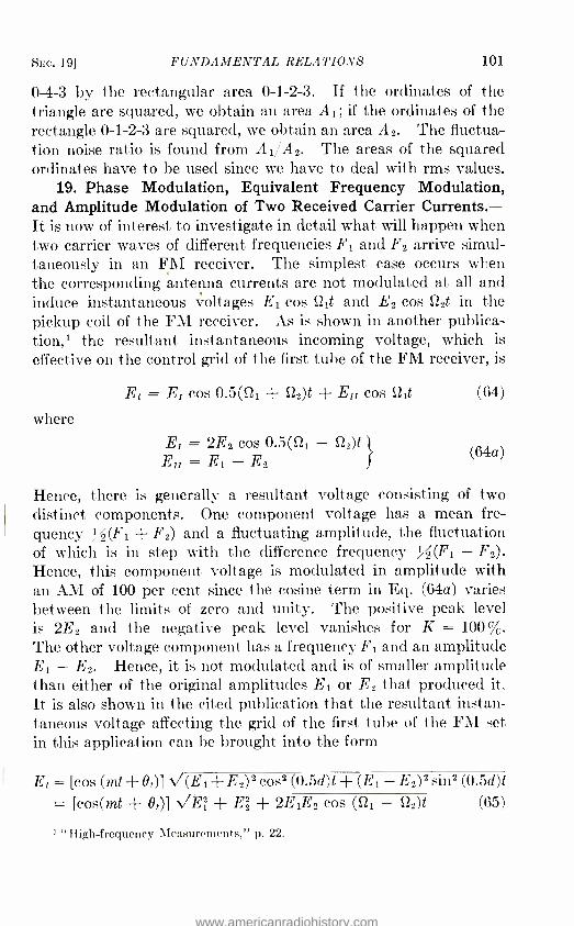
SEC. 19] FUNDAMENTAL RELATIONS 101
0-4 -3 by the rectangular area 0- 1 -2 -3. If the ordinates of the triangle are squared, we obtain an area Al; if the ordinates of the rectangle 0 -1 -2 -3 are squared, we obtain an area A2. The fluctua- tion noise ratio is found from A1/A2. The areas of the squared ordinates have to be used since we have to deal with rms values.
19. Phase Modulation, Equivalent Frequency Modulation, and Amplitude Modulation of Two Received Carrier Currents. - It is now of interest to investigate in detail what will happen when two carrier waves of different frequencies F1 and F2 arrive simul- taneously in an FM receiver. The simplest case occurs when the corresponding antenna currents are not modulated at all and induce instantaneous voltages E1 cos S21t and E2 cos S22t in the pickup coil of the FM receiver. As is shown in another publica- tion,' the resultant instantaneous incoming voltage, which is effective on the control grid of the first tube of the FM receiver, is
Et = E, cos 0.5(1 + S22)t + E11 cos 1.21t (64)
where
EI = 2E2 cos 0.5(12, - S22)t (64a) E =E1 -E2 f
Hence, there is generally a resultant voltage consisting of two distinct components. One component voltage has a mean fre- quency ;(F1 + F2) and a fluctuating amplitude, the fluctuation of which is in step with the difference frequency ¡2(F1 - F2). Hence, this component voltage is modulated in amplitude with an AM of 100 per cent since the cosine term in Eq. (64a) varies between the limits of zero and unity. The positive peak level is 2E2 and the negative peak level vanishes for K = 100%. The other voltage component has a frequency F1 and an amplitude E1 - E2. Hence, it is not modulated and is of smaller amplitude than either of the original amplitudes E, or E2 that produced it. It is also shown in the cited publication that the resultant instan- taneous voltage affecting the grid of the first tube of the FM set in this application can be brought into the form
Et= [cos (mt + et)] V'(E1 +E2)2 cose (0.5d)t + (E, - E2) 2 sine (0.5d)í
= [cos(mt + Os)] VE? + E2 + 2E1E2 cos (121 - S22)t (65)
' "High- frequency Measurements, p. 22.
www.americanradiohistory.com

102 FREQUENCY MODULATION [CHAr. I
where
m = ¡+
Q2); d = 1-21 - Sl2; ll
BL = tan-1 f E1 E2 tan [0.5(Sì, - 122)t] } 1E, + E2 1
Hence, in addition to AM between the limits E1 - E2 and E1 + E2, we have also phase modulation since Eq. (65) has the form
Et = Em, cos {[0.5(Sí, + S22)]t + O,} (66)
No assumptions were made in the derivation of Eq. (66), which holds for any values of F, and F2 as well as for any values of E1 and E2 that may occur in practice. The argument a = 0.5(SZ, + S22)t + B, gives, therefore, a means for computing the equivalent FM from the relation
t
F, = 2r dt = 0.5(F1 + F2) + 27r dt (67)
(65a)
The differentiation of dOt /dt is conveniently done after the values of the amplitudes E, and E2 and F, and F2 have been inserted in the formula for O, given in Eq. (65a). The angle O, can also be obtained from the first relation for Et given in Eq. (65). It is necessary only to plot the value (E1 -{- E2) cos cp along the X axis and the value (E1 - E2) sin yo along the Y axis of a rectangular coordinate system for yo = 0.5(521 - Sì2)t where the corresponding difference frequency is half the value of F1 - F2, although in the second relation of Eq. (65) it will be noted that the actual differ- ence frequency F1 - F2 plays a part. Suppose these quadrature components are plotted and we find, for instance, that at the instant of time which makes 0.5(52, - S-12)t = 45 deg, we have sin cp = cos cp = 0.7071 and 0, = tan-' [(E1 - E2) (E, -f- E2)]. Hence, for equal amplitudes of the incoming currents in the aerial, there would be no phase deviation at this instant; for E2 = 0.5E, we would have 0, = i: and an instantaneous phase swing 0, = 18.4 deg. Hence, when two unmodulated currents of different carrier frequencies and with any amplitude relationship affect the grid of the first tube of an FM receiver, we have the case of a íwofold modulated current, namely, AM + PM, which can also be interpreted as AM with simultaneous equivalent FM as far as the actions in the discriminator are concerned.
www.americanradiohistory.com

SEC. 14 FUNDAMENTAL RELATIONS 103
The most important thing is not the AM, since an amplitude limiter can prevent such modulation from reaching the discrimina-
1 d®, tor, but the instantaneous equivalent deviation frequency
- 27 dt
It is this term which affects the output current of the discriminator. We note from the expression for Ot in Eq. (65a), that there will be equivalent frequency swings as long as there is a time function in any of the terms that make up the value of the relative phase et.
Hence, it is the factor 521 - 522 in the Ut relation of Eq. (65a) that partly determines the degree of PM and, therefore, also the degree of equivalent FM as experienced by the discriminator. Hence, when the arriving unmodulated waves have exactly the same carrier frequency (F1 = F2), then S21 - 522 = 0 and there can be no PM and, therefore, no effects in the discriminator of an FM receiver. Moreover, when the difference between the respective carrier frequencies is relatively small, the degree of PM is also small and, consequently, the equivalent FM likewise must be small. It appears, therefore, from this discussion that a great difference exists when FM reception is compared with AM recep- tion. An AM receiver would, for small frequency differences that are in the a -f range, produce decided beat- frequency interference since, according to the last square -root expression of Eq. (65), the AM produced in the resultant voltage causes audible amplitude variations of beat frequency F1 - F2. Besides, when frequency equality exists and one voltage is the desired voltage and the other is an interference voltage, the amplitude ratio E1 /E2 will show to what extent the interfering wave blanks out the desired wave. Hence, when each arriving wave is a modulated wave, the AM receiver will experience considerable interference in com- parison with such effects in an FM receiver.
Since, according to the first expression of Eq. (65), the resultant amplitude has a cosine part with an amplitude value of E1 + E2 and a sine part with a value of E1 - E2, it is seen that, at any instant when 0.5(21 - S22)t = 0 deg, the sine term vanishes and the amplitude of the resultant is E1 + E2; at an instant when 0.5(521 - S22)t = 90 deg, the resultant voltage must be E1 - E2 since the cosine term vanishes. Hence, the AM occurs between the limits E1 - E2 and E1 + E2 and for equal arriving amplitudes we have 100 per cent modulation.
www.americanradiohistory.com

104 FREQUENCY MODULATION [CHAP. I
When we tune to a desired station, we emphasize the cor- responding desired current D sin Olt that circulates in the input network of an FM receiver; an interfering station must cause a much smaller amplitude I in the interfering current I sin 522t.
The superposition of these two currents gives then a solution similar to that used in connection with Eq. (65), since for the substitution S2 = S21 - ,G2
It = D sin 521t + I sin S22t = D sin Slit -+ I sin S21t cos SZt
+ I cos S21t sin Sgt
= (D + I cos Sgt) 'sin S21t + (I sin SZt) cos S21t
a
(1t = a + jb = ßa2 + b2 sin + tan -' b/ a or
It = 1/D + I + 2D1 cos (521 - S22)t sin S2it + tan- I sin (12,- S22)í 2 2
1 [
{ I cos (S2e - S22)t = I,,, sin at (68)
holding for any amplitude ratio D/I and any frequency ratio F1 /F2. In our receiver, for unequal frequencies F1 and F2 and for selective tuned circuits', I is much smaller than D. This is usually true also for present-day allocation of stations on the same channel (F1 = F2) where the stations are almost certain to be so located that only the desired wave provides a strong signal field intensity. Therefore, the expression for both the instantaneous value of the amplitude Im, and the instantaneous angle at can be simplified. Hence, for I, small in comparison to D, we obtain the approximations
Ime = D [
1 + D
cos (521 - U2)tl
at = U1t + 15 sin (S21 - 02)t
and
It = D I 1 + ib cos (01 - S22)tj sin [1t + T)
sin (01 - S22)t]
(69)
(70)
Comparing this result with the customary AM + PM case for which we have
It = I,, (1 + K cos wt) sin (Ut + 0O sin wt) (71)
www.americanradiohistory.com

SEC. 19] FUNDAMENTAL RELATIONS 105
we note that we have now an AM of degree K = I /D, as was found above, and a superimposed PM with a maximum phase swing I/D which is controlled by a sine function of the beat frequency F1 - F2
instead of by the signal requency f. Since the time rate of change dat /dt of the at approximation given in Eq. (69) and employed in Eq. (70), when multiplied by 1/6.28, gives the instantaneous value of the equivalent carrier frequency, we find
Ft = F1 -D (F1 - F2) cos (S21 - S22)t (72)
Since F1 is the fixed carrier frequency of the incoming desired current D sin (6.28F,)í, the factor I(F1 - F2) /D is the equivalent
PZ
n,
P,
\
D is desired current I is interfering current
P3
-/evel
b D- level
Caps a -b -c Clipped-off'
L -level a
Useful At-variation
1
level
D -level FIG. 28.- Diagram for two received unmodulated carriers of different frequencies
S21/6.28 and t2 /6.28.
maximum frequency deviation due to the PM produced by the interference. Hence, the amplitude of the corresponding fre- quency excursions is also proportional to the difference frequency Fi - F2, but, in addition, depends on the amplitude ratio I /D. This shows that the frequency discriminator cannot be affected at all by the equal carrier frequencies of the two incoming unmod-
www.americanradiohistory.com
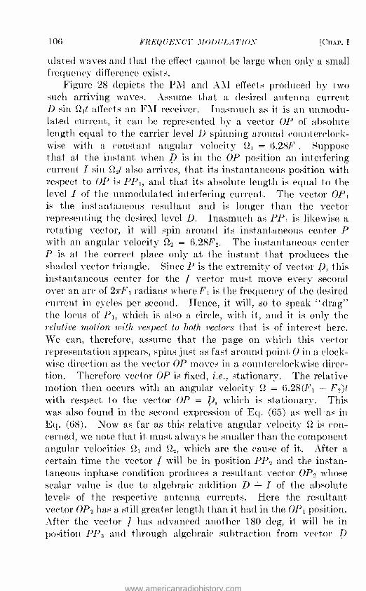
106 FREQUENCY MODULATION [CHAP. I
ulated waves and that the effect cannot be large when only a small frequency difference exists.
Figure 28 depicts the PM and AM effects produced by two such arriving waves. Assume that a desired antenna current D sin S2,t affects an FM receiver. Inasmuch as it is an unmodu- lated current, it can be represented by a vector OP of absolute length equal to the carrier level D spinning around counterclock- wise with a constant angular velocity SZ1 = 6.28F . Suppose that at the instant when D is in the OP position an interfering current I sin S22t also arrives, that its instantaneous position with respect to OP is PP1, and that its absolute length is equal to the level I of the unmodulated interfering current. The vector OP, is the instantaneous resultant and is longer than the vector representing the desired level D. Inasmuch as PP1 is likewise a rotating vector, it will spin around its instantaneous center P with an angular velocity 122 = 6.28F2. The instantaneous center P is at the correct place only at the instant that produces the shaded vector triangle. Since P is the extremity of vector D, this instantaneous center for the I vector must move every second over an arc of 27rF, radians where F1 is the frequency of the desired current in cycles per second. Hence, it will, so to speak " drag" the locus of P1, which is also a circle, with it, and it is only the relative motion with, respect to both vectors that is of interest here. We can, therefore, assume that the page on which this vector representation appears, spins just as fast around point 0 in a clock- wise direction as the vector OP moves in a counterclockwise direc- tion. Therefore vector OP is fixed, i.e., stationary. The relative motion then occurs with an angular velocity St = 6.28(F1 - F2)t with respect to the vector OP = D, which is stationary. This was also found in the second expression of Eq. (65) as well as in Eq. (68). Now as far as this relative angular velocity St is con- cerned, we note that it must always be smaller than the component angular velocities SZ, and S22j which are the cause of it. After a certain time the vector I will be in position PP2 and the instan- taneous inphase condition produces a resultant vector OP2 whose scalar value is due to algebraic addition D + I of the absolute levels of the respective antenna currents. Here the resultant vector OP2 has a still greater length than it had in the OP' position. After the vector I has advanced another 180 deg, it will be in position PP3 and through algebraic subtraction from vector D
www.americanradiohistory.com

SEC. 19] FUNDAMENTAL RELATIONS 107
(because of the instantaneous antiphase condition) will produce a resultant vector OP3 which has a level of only D - I. Hence, during the complete beat -frequency cycle, we have an AM between the level limits D -I and D + I, and a degree o_ amplitude modu- lation K = 100I /D per cent. The unmodulated current of smaller level behaves, therefore, like a modulating current I sin (S21 - S22)t,
which causes AM. From the figure it will be noted that the resultant vectors OP4 and OP5 show extreme ,out -of -phase con- ditions, with exactly the same negative and positive phase 5
with respect to the desired vector OP = D. This is the PM effect with the corresponding maximum phase swings ±M. According to Eq. (70), we have M = I/D for a small ratio of I /D. Since the relative vector spin of I occurs along a circle with the uniform angular velocity S21 - S22 of the beat frequency, the equivalent maximum frequency deviation produced must be equal to (F1 - F2) M where M is in radians. Since both AM and PM, as well as the equivalent FM, are caused by the incoming currents D sin 21t and I sin S22t, they give a means for determining in a simple way the maximum phase swing M. Both currents have to be added in quadrature since they are of different fre- quencies, namely, F1 and F2. Hence, the resultant level must be D + jI with a maximum phase swing AB = tan' (I /D). For example, for I = 0.2D we have M = ± 11.3 deg maximum phase swing during the modulating cycle of frequency F1 - F2. The magnitude of this phase swing is. independent of the frequency difference F1 - F2. This angle corresponds to 11.3/57.3 = 0.197 radian, giving an equivalent frequency swing of 0.197(F1 - F2). If the frequency difference were 100 kc, we would have an equiva- lent maximum frequency excursion of 19.7 kc and for a 1 -kc frequency difference we would have an equivalent frequency swing of only 197 cycles per second. For F1 = F2 there is no PM at all and, therefore, also no equivalent frequency swing due to interference that can affect the discriminator output.
Now in AM receivers the ratio of the a -f interference to the useful audio signal is generally equal to the ratio of the h -f inter- ference voltage to the useful h -f voltage applied to the detector. These respective voltages are the ones applied from the output of the last i -f stage to the amplitude demodulator.
But in an FM receiver the stronger of the two modulated currents has a tendency to remove the weaker one (on account
www.americanradiohistory.com

108 FREQUENCY MODULATION [CHAP. I
of the I/D effect in Eq. 70). Hence, when examining two FM carriers, we can, as in Fig. 28, again add vectorially the desired signal vector D to the interference vector I and find the resultant R as in Fig. 29. The respective FM's cannot affect the length of these vectors, since they still will be equal to the respective carrier levels D and I if the two received currents are D sin (S21t + ß sin wt) and I sin (S22t + )3' sin w't), where ß' and w' express the fact that the intensity of FM and the frequency w'/6.28 of the modu- lating signal do not have to be the same for the interfering
current and the desired FM signal cur- rent. At the instant shown, vector D has advanced an angle (pi with respect to the reference axis; I has advanced an angle g tp2 j and the instantaneous resultant vector R now represents a larger level and has a relative phase advance cp. Since D is now frequency modulated, it no longer spins counter- clockwise with a constant angular
Reference axis FIG. 29.- Resultant effect of
two frequency -modulated cur- rents of different center frequency.
velocity S21, but in addition experiences an oscillatory angular velocity swing about S21 since the corresponding instantaneous carrier frequency
is now F1 + OF cos wt. For the interference vector, a similar superimposed oscillatory swing occurs since the vector I has an instantaneous carrier frequency F2 + OF' cos w't. Also, in the vector representation of this figure, the maximum angle between the resultant R and the desired vector D can never exceed an angle of tan-1 (I /D). For an interference level I equal to half the value of the desired carrier level D, this angle is tan-1- 0.5 = 26.6 deg, irrespective of the instantaneous beat frequency of F1 + OF cos wt - F2 - OF' cos w't. The frequency modulation of the desired
current vector is therefore - -', the frequency modulation of
the interference vector is 1
42, and the FM of the result- 2r dt 1 chp ant vector R, which will affect the discriminator output, is
Hence, even though the angular variation of the interference vector I were several thousand degrees, it could hardly cause much
www.americanradiohistory.com

SEC. 19] FUNDAMENTAL RELATIONS 109
change in since this angle cannot exceed a value of 45 deg even for I = D.
Suppose the desired current D sin 121t has a deviation ratio OF /f = 15 due to a maximum frequency swing of 75 kc and a
signal frequency f = 5 kc. We have, then, equivalent phase advances and retardations of 15 X 57.3 = ± 859.5 deg and, therefore, several complete revolutions during one modulation cycle for either the desired vector D or the resultant vector R.
Therefore, the interference I cannot affect the resultant FM very much as long as D is greater than I during all portions of the modulation frequency cycle.
In order to obtain an idea of how much more effectively FM avoids interference than does AM, reference is made here to Eqs. (70) and (72). Equation (70) shows that in an AM receiver the interference I causes a degree of modulation equal to K = I /D, where D is the amplitude of the desired current. The modulation conversion from FM into AM in a discriminator, even for the most ideal translation, is equal to the peak -to -peak frequency excursion divided by the channel width w. Since the discriminator is
designed for the very maximum peak -to -peak frequency swing,
i.e., 2 X 75 kc, the channel width is 150 kc or 2 OF where OF is
the largest permissible frequency excursion. Now, from Eq. (72)
we note that the equivalent frequency swing is I(F1 - F2) /D. Hence, the peak -to -peak frequency swing is equal to twice this value and the FM to AM translation gives an equivalent AM of a
degree
K - (F1 - F2)I D F
which when multiplied by 100 gives K in per cent. We have, therefore, the comparison:
I D
F1 F2 D OF
Interference modulation in an AM receiver
Interference modulation in an FM receiver for AF as the largest permissible frequency devi- ation ( ±75 kc)
These formulas show that for AM the ratio of interference level I to desired carrier level D determines essentially the intensity of the a -f interference heard in an AM receiver. In other words,
(73)
www.americanradiohistory.com

110 FREQUENCY MODULATION [(H :r. I
the desired carrier level has to be high enough with respect to the interference level to "drown out" the interfering sound. How- ever, for an FM receiver we have, in addition to this ratio, which should also be small (since the formulas are based on such assump- tions), a factor (F1 - F2) /OF which shows that for equal carrier frequencies (F1 = F2) for the interfering and desired signals no interference is possible at all; for a small difference of F1 - F2 not much interference can exist; for the highest audible beat frequency (F1 - F2 = 15 kc) that can be handled and heard in an FM receiver, the factor (F1 - F2) /OF still causes a reduction of interference. For AF = ±75 kc this factor is equal to 0.2 and the resulting interference in an FM receiver would be only 20 per cent of that obtained with an AM receiver. Fortunately, matters are even more favorable, since in properly designed FM receivers the a -f emphasis in the upper a -f range employed i:i FM transmitters is compensated by a corresponding frequency deemphasis in the receiver, also in the upper a -f range. Hence, an audio frequency as high as 15 kc due to interference modulation will also be deemphasized. Moreover, for a 2 -kc tone due to F1 - F2, we have (F1 - F2) /OF = 275 = 0.0267 or only 2.67 per cent FM interference as compared with the corresponding inter- ference in an AM receiver. We note also in Eq. (73) that wide - band FM, i.e., large OF values, avoids more interference.
20. Superposition of Currents in Transfer Networks. -Suppose we have to deal with the superposition of two currents A sin S21t
and B sin S22t in any FM transfer network. The vectorial addition of A + B at any instant will lead to a resultant instantaneous vector R, which has a relative phase O with respect to the reference axis shown in Fig. 30. We have, therefore, no longer phases of zero and cp as for the respective component vectors.
Four possible cases can be distinguished. For case 1, both component vectors revolve with the same constant speed S2 = S21 = S22. We have then the relationship depicted in Fig. 30 with a phase angle O which is equal to an inverse tangent function of the phase difference cp between the component currents of respective amplitudes A and B, and the amplitudes A and B themselves. For such conditions there can be neither amplitude modulation nor phase modulation as well as no equivalent frequency modula- tion. But it is of interest to note that even though the instan- taneous relative phase Br = O is fixed, it can be the result of ratios
www.americanradiohistory.com

SEC. 20] FUNDAMENTAL RELATIONS 111
B sin cp,i (A + B cos cp) which may have any value from minus infinity to plus infinity. Hence, the tangent function is not so convenient a variation for practical applications as are the sine and cosine functions, which vary only between the limits -1 and +1. This statement will be evident if we realize that in FM systems we are not interested in a fixed phase but in a variable phase 91. This phase is then either an equivalent phase variation for direct FM or is a true phase variation in case of PM. Each of these two possible conditions will produce corresponding
7
6
5 4 3
2 X 1
C3 0 C
-2 -3 -4 -5
6
-7
+00 +oo +oo f 4
CÌ
I
I' I Ì Ì -- - -Ian e
Ian B
I
' ' _. - I
: Ì. _
Brádiánsi 2 = '
2I C
q
z,-1 Ì :r 3rr
2
5n C3rr 2-
I
I a
fan B on B I
III t II I iI
I 1 I II II II 1
1 11 11 -03 -CO
Reference I
axis n íSLBsin
c.04
t''- q r
2
B
Resullanl R=A+B cos p+jBsin g
B=1añLr+*BcosI kn 1X
Xradians ® for X<0.2 N57.3Xdegrees
FIG. 30.- Behavior of resultant relative phase deviation when two electromagnetic waves with different center frequency and modulation arrive.
responses ill the output branch of a frequency discriminator. But, fortunately, we note that also here portions of the tangent function, for instance, between 1 and 2 of Fig. 30, refer to "linear" variations. This linear relationship between the value of the relative phase of the resultant current and the value of X prevails for values of X < 0.2.
Since for the other cases that will be described later the value of X is by no means constant, we should realize that the inter- sections of the successive tangent curves with the O axis are the most suitable operating points for satisfying a linear relation. This is true because they are mid -points along the straight portions of the tangent curves. They are also points of "inflec- tion" that can be found from any expression for the value of X by setting the second derivative d20 of the relative phase with respect to the variable in the expression for X equal to zero.
www.americanradiohistory.com

112 FREQUENCY MODULATION [CHAP. I
Hence, for case 1, this would generally mean that d20/dX2 = O.
This will lead to points O = 0, ir, 27r, 37r, etc. However, in the expression for X there are three quantities that can affect the result if variation of any of these quantities should take place. One is the amplitude A of one component current, the second is
the amplitude B of the other component current, and the third is the phase difference cp between the component currents. Hence, if amplitude A should undergo variations, we find the most suitable operating points from d2B /dA2 = 0; for amplitude modula- tion of the carrier B sin Slit we find the operating point from d20/dB2 = O. The third possible variation is when the phase difference cp varies; then we have the relation d20/42 = 0 for finding the operating point.
Inasmuch as the angle O of the relative phase of the resultant current depends on A, B, and so, any desired as well as parasitic variations in any of these factors must produce modulations in the resultant current. We can, therefore, generally say that for the superposition of two currents there is a tendency for producing a variation in the value of the relative phase O. But this is PM and, consequently, also equivalent FM. Even though the component currents are primarily fixed in amplitude and in relative phase, at least as far as the corresponding voltages that cause them are concerned, a transfer network, in virtue of its impedance, may cause such modulations. This will happen if the network does not have a linear phase shift for all frequencies of the band width that play a part. For nonlinear phase responses the relative phase cp cannot remain constant. In addition there must be impedance actions of the transfer network such that equal current amplitudes result for all frequencies of the band width when one and the same voltage amplitude, but of any frequency in the band width, is applied. This will satisfy the condition that neither A
nor B be altered owing to the action of the transfer network. Case 2 refers to the general application that concerns us in
FM systems. It is when both component currents are modulated in amplitude. This could be due to a condition such that the amplitude response of the transfer network is not flat over the entire band width. For instance, an i -f network has an impedance characteristic with respect to the frequency, which increases near the lower and upper cutoff frequencies; or the characteristic, when due to overcoupled tuned circuits, is such as to cause a
www.americanradiohistory.com

SEC. 201 FUNDAMENTAL RELATIONS 113
lower response near the mid -frequency of the pass band. Hence, generally for this case we no longer have constant amplitudes A and B, but A + a(t) and B + b(t) where a(t) and b(t) indicate any time functions that may occur due to such defective transfer characteristics. A simple variation would be a cos wt and b cos wt
causing currents (A + a cos wt) sin Stit and (B + b cos wt) sin SZIt,
respectively. It is always correct to use a(t) and b(t) where (t) stands for any time function that satisfies the amplitude frequency characteristic of the transfer network. Doing this we find, instead of the O = tan-1- X formula of Fig. 30, the expression
0t = B Dot =tari 1 [B + b(t)] sin cp l
{A + a(t) + [B + b(t)] cos = tan- [X(t)] (74)
showing that generally there is no linear phase deviation in the relative phase 0t with respect to the time function (t). Even this is not always true for values of the ratio under the tan-1 bracket < 0.2. Nevertheless, this relation must have a portion on the corresponding tan 0t curve for which Ot = ko + k(t) holds; i.e., a portion for which the variation in the variable portion of 0t is directly proportional to the time function (t), the constant of proportionality being k, since ko accounts only for the fixed portion O of the relative phase. The most suitable operating point is again the mid -point of the linear portion of the cor- responding curve of X(t) plotted against 0t. The operating point is then found as above from d20í /d(t)2 = 0. Doing this, we find a solution of the form
d20` mp 0
d(t)2 q
where either factor m or factor p must be zero in order to render mp /q = 0 as necessary for the determination of the most suitable operating point. Hence, in the second differentiation it is only necessary to evaluate the numerator mp. Doing this we find that m no longer contains the time function (t) and, therefore, cannot cause PM. Hence, the factor
p = Bbsin2cp -F (A +B cos (p)(a +b cos cp)
+ [ (a + b cos cp) 2 + b2 sine cp] (t) = 0 (76)
is to he used in the evaluation for the operating point. This expression will be greatly simplified if we realize that for the oper-
(75)
www.americanradiohistory.com

114 FREQUENCY MODULATION [CHAT'. I
ating point there can be no phase modulation since the phase variations take place about this point. No PM will occur when all terms affected by the modulation function (t) disappear. Hence, for the operating point we obtain
Bb sin2 cp + (A + B cos (p) (a + b cos cp) = 0,
or
Aa + Bb cos cp _ - Ab + Ba - -n (76a)
We are not interested in the steady or fixed component O of 0,
about which phase swings take place, but only in the instantaneous phase swings or phase deviations themselves. Hence, d0, /d(t) is the expression to use for finding these swings, and we have
do, [b(A + B cos (p) - B(a + b cos (p)] sin yo
d(t) [(A + B cos cp) + (a + b cos (p) (t)] 2 + [B sin so + (b sin ) (t)] 2
For the operating point all terms with the variable (t) function must vanish, and therefore
d0, [b(A + B cos so) - B(a + b cos (p)] sin cp
d(t) (A + B cos cp)2 + B2 sin2 (77) operating
point
Since Eq. (77) holds for the operating point, it must be satisfied by Eq. (76a). We find for the numerator of Eq. (77)
[b(A - nB) - B(a - nb)] sin cp = (bA - Ba) sin yo (77a)
and for the denominator, by squaring, the relation
A2 + B2(cos2 cp + sing (p) + 2AB cos yo = A2 + B2 + 2AB cos So
(77b)
The instantaneous phase excursion then becomes
O0, = tari 1
yo (t) l
= tan' [p(t)] (78) A2 +B2 +2AB cos So
Hence, for values of p(t) < 0.2 we may expect linearity; i.e., the phase swings will be proportional to the time function (t) that causes the PM. For such values, we will have the formula
(bA - Ba) sin yo - (79) B' A2 + B2 + 2AB cos yo
www.americanradiohistory.com

SEC. 20] FUNDAMENTAL RELATIONS 115
This is a very general formula since almost any time function can be substituted for (t). For a sinusoidal AM effect of im sin wt we have (t) = im sin wt and linear response takes place as long as imp
does not exceed values of 0.2. Case 3 refers to a condition for which the vector A has no
modulation and has the form A sin Sgt, while the vector B is partly modulated in amplitude and is of the form
(B + bi,,L sin wt) sin (Stt + (p);
i.e., it is applied with a phase of cp with respect to the completely unmodulated carrier A sin Slt.
Case 4 refers to a condition where a completely modulated modulation product (KIm sin wt) sin (S2t + so) is added geo- metrically to an unmodulated carrier Im sin Sgt. Such a scheme was briefly mentioned on page 6 in connection with Fig. 3.
If so is 90 deg, we have the case of Fig. 3.
From this discussion it is seen that poorly designed transfer networks will cause PM owing to amplitude distortion and will, consequently, also produce equivalent FM effects. For instance, for the case where the time function (t) in Eq. (79) is equal to im sin wt, the equivalent frequency swing will be
1 d(M) 27r dt -fp cos wt
In a similar manner, expressions can be derived in which a non- linear phase shift with respect to the pass frequencies causes "directly" a change in the value of cp. The discussion in con- nection with the explanations given in Fig. 28 shows also that when two or more interference pulses enter the band -pass transfer networks simultaneously, there will be mutual modulation effects, even though each pulse by itself would cause no effects at the output of a balanced frequency discriminator. The mutual effects cause PM and equivalent FM. The strongest PM effect will occur when both disturbances have the same mean frequency' and one interference is, in equivalence, 90 deg out of phase with respect to the other interference. As a matter of fact this may happen whenever recurrent disturbances overlap. It also happens when a useful modulated carrier acts at the mean frequency of a simultaneous pulse interference and if the interference produces
1 For details, consult Sec. 21, p. 117.
www.americanradiohistory.com

116 FREQUENCY MODULATION [CHAP. I
a larger equivalent amplitude than does the signal modulated carrier. The discriminator will then register chiefly the noise at its output.
21. Different Kinds of Interference Impulses. -In connection with Fig. 27 we have already discussed how much less sensitive FM receivers are to the interfering effects of fluctuation or random noise than are AM receivers. By fluctuation noise is usually understood such noise as is experienced in receivers with very high amplification. It is often also called interchannel noise. This noise causes a continuous distribution of random h -f currents, which do not have a fixed relative phase relationship. This is the reason why, for such distributions, the rms method was used in connection with the amplitudes of the noise areas in Fig. 27, which led to the second comparison formula of Eq. (63). Since for an AM receiver the band width is equal to twice the maximum signal frequency fm., which is normally taken as 15 kc, and, according to Fig. 27, the height 0 -1 is constant for the total band width 2fm., the sum of the squared amplitudes for this band width is likewise constant. Hence, fluctuation noise must be propor- tional to the factor ` fmax for an AM receiver while for an FM receiver, according to Fig. 27, we have a slope 0 -4 instead of the horizontal 1 -2. This leads to the comparison for a constant k
Fluctuation or random noise
('rmaa 212 CL[F1 - F2] /y,
!I J J /{,f msx
/3 OF f msx for FM (80)
k 1/f for AM I
Strong noise impulses of very short duration will usually cause an energy distribution over the entire band width of the i -f net- works. The duration spread in Fig. 31a is inversely proportional to the band width. Hence, in wide -band FM we have approxi- mately the distribution indicated in Fig. 31a when a single sharp impulse acts on a band -pass transfer network having a lower cutoff frequency F2 and an upper cutoff frequency F1. Therefore, the resultant current depends upon both cutoff frequencies used in the i -f networks. As an approximation, as far as the explana- tion is concerned, the envelope or amplitude curve is filled up with a h -f current of center frequency F = 0.5(F1 + F2) of the pass
www.americanradiohistory.com

SEC. 211 FUNDAMENTAL RELATIONS 117
band. Even though the energy is mostly under the center portion or peak envelope contour of Fig. 31a, as far as the spread as applied to the discriminator is concerned, it is more or less uniform, as is shown in Fig. 31c. Only the shaded portion 2fmax wide will be heard as interference noise. Hence, a balanced discriminator will produce in each half of its circuit, at the same instant, opposite output voltages with zero voltage as the net result. That is what
sin[2rr(F,-fl/I_A 1m /
(a) A unit impulse applied to an ideal band pass filter
r
fAmpli/ude
(c)
Uniform energy
F-75 kc F-15kc F F+15kc F+lSkc
F= 05154-F27
Ampli/ude
---df[/m[sin[2ef-F4h}dA (d) I d/ ,-/-/-
I
II Time F-l5kc F-15kc F F+15kc F+75 kc
FIG. 31. -Unit impulse (a) causes uniform energy distribution while the derivative (b) of unit impulse causes energy distribution (d).
occurs when certain impulses enter the i -f stages and subsequently, after passing the limiter, affect a balanced discriminator. But, when a useful FM signal, which has the same mean frequency also exists, PM due to mutual effect can result, especially when quadrature addition as shown in Fig. 3 takes place. The stronger of the two currents will then be the one that mostly affects the output of the discriminator. The higher the initial peak (center peak) shown in Fig. 31a, the more phase shift, and, therefore, also equivalent frequency shift, will be produced in the desired FM
www.americanradiohistory.com

118 FREQUENCY MODULATION [CHAP. I
wave. But the limited band width of 2 OF often checks such tremendous frequency excursions as far as the output effect is concerned. Figure 31b shows the derivative of the unit pulse shown in Fig. 31a. Such differentiations take place when induc- tive coupling is used, since the driving voltage M di /dt transfers the pulse energy into the circuit that is coupled to the circuit carry- ing the current i. Figure 31d shows the energy distribution, which is even more favorable than for the pulse of Fig. 31a. Figure 32
Unit step pu /se At
Infinity A
Unit i
pulse
dAt dt
Y
Amplitude
fmax Energy distributibn for unit step pu /se
F F+15kc
Amplitude
Energy distribution for unit pu /se
F+75 kc
F F +15kc Fin. 32.- Impulses and their noise distributions.
depicts energy- frequency distributions for a unit step pulse and its derivative.
As far as the action in a band -pass network is concerned, a sudden disturbance, as just illustrated, can be defined by the expression A (t) sin [27rFt + 0(t)], where F stands for the center frequency of the pass band.
22. Frequency Multiplication in FM Systems. -We have to dis- tinguish three typical frequencies in FM systems: the instan- taneous carrier frequency F1, the maximum deviation frequency OF, and the signal frequency f, which is also known as the frequency of the current that modulates. The signal frequency in high - fidelity work should remain the same as at the input of the modula- tor of the transmitter and, therefore, requires no multiplication or change. Only multiplication of the instantaneous carrier fre- quency F, and of the maximum deviation frequency OF is needed. In present -day FM transmitters the primary FM source is not
F+75kc
www.americanradiohistory.com

SEC. 22] FUNDAMENTAL RELATIONS 119
wide -band FM as in the final transmitted electromagnetic wave and multiplication of the primary frequency deviations is necessary.
Inasmuch as the deviation frequency AF cos wt, at any instant of time, is equal to the difference between the instantaneous carrier frequency Ft and the center frequency F, a multiplication of the instantaneous carrier frequency Ft means that the deviation frequency AF is multiplied also and by the same factor as is Ft. In indirect FM, as in the Armstrong transmitter, the value of Ft is the outcome of an equivalent frequency swing M cos it about a fixed carrier frequency F. The phase modulation n the Arm- strong system causes (M /f) sin wt phase swings and in turn equivalent f(OB/I) cos wt frequency deviations. This behaves exactly like the actual instantaneous carrier frequencyF + AF cos wt in case of direct FM, since for indirect FM for all signal fre- quencies f, we have AO = F, if the constant of proportionality is taken as unity.
The requirement for the frequency multiplier is, therefore, that the input as well as the output network handle all spectrum currents' due to currents of frequencies F. The output pass band must be equal to the width of the input pass band times the order of frequency multiplication. In indirect FM successive frequency multiplication is used with an intermediate network, which causes a difference- frequency or center- frequency conversion, because a much larger frequency deviation multiplication is needed than the corresponding carrier frequency multiplication. In direct FM comparatively large frequency swings can be produced directly in the primary FM oscillator and a much smaller deviation frequency multiplication is needed. In direct FM, therefore, the center -frequency multiplication is of the same order as the devia- tion frequency multiplication. For instance, in the RCA trans- mitter, as well as in the FM transmitter of the General Electric Company, two frequency tripiers are used. This means that, on account of a ninefold frequency multiplication, the final output network has to be designed for a band width somewhat wider than required by the maximum peak -to -peak frequency swing. Since this maximum peak -to -peak output swing is never more than 2 X 75 = 150 kc, at the input side of the last tripler it is 15% 3 = 50 kc. It has this same value at the output of the first tripler and
It should he recalled that it is the number of significant side currents and not the instantaneous carrier currents of frequencies F, that determines the band width.
www.americanradiohistory.com

120 FREQUENCY MODULATION [CHAI'. I
is equal to 5% 3 = 16.67 kc at the input side of the first tripler. Hence, the largest permissible maximum frequency excursion in the primary FM will not exceed ± 8.335 kc. Since the maximum deviation ratio 7%5 = 5 = ß causes the widest pass -band spread, we find from Table III that the total band width is 16f = 16 X 15 = 240 kc for the final output network of the FM transmitter. This is also the band -width requirement for an FM receiver, which applies, of course, also to the i -f stages. It is, however, customary to design these networks for a band width of only 225 kc. At the input side of the last tripler, as well as at the output side of the first tripler, we have a permissible maximum frequency deviation of 7% = 25 kc. The corresponding maximum deviation ratio is 2%5 = 1.667 = ß, requiring a band -width design for only eight significant side currents. Hence, a width of 8f = 120 kc is needed. For the input side of the first tripler we have a maximum deviation ratio that is only one -ninth as large as in the antenna current or only % = 0.556 = ß. This requires, according to Table III, a band -width design of about 4f or 60 kc. The present -day Western Electric FM transmitter uses only eightfold frequency multiplication by means of three frequency doublers in cascade. Details of these arrangements are described in Secs. 23 and 47.
In the Armstrong system shown in the block diagram of Fig. 33, a stabilized 200 -kc primary frequency F1 is used for controlling the ultimate center or mean frequency F of the radiated electromag- netic FM wave. Since, in this system, theoretically we should not go over a maximum phase swing of more than 0.2 radian if harmonic distortion is to be avoided,' the value of M/f should never exceed 0.2 radian. Hence, it is the lowest desired signal frequency that determines the equivalent deviation frequency multiplication necessary. Since for indirect FM the value of AO
expressed in radians is equal to OF in cycles per second, because the ratios M/f and AF /f must be the same in this case, we can readily determine what is the lowest signal frequency f for which
Figure 3 shows that for maximum phase angles of such a magnitude that the modulation product, i.e., the quadrature amplitude b, does not form a portion of the circle of radius a, we have also superimposed AM. In Fig. 3b, OP = a; PPI = b.
It is true that we can remove this parasitic amplitude modulation, hut we should bear in mind that for PM + AM we have also so- called "theoretical" cross- spectrum effect; i.e., even though an amplitude limiter can readily remove the AM effect, it is still part of the modulation energy, and the receiver that responds only to FM will miss certain components, which were removed, and will produce distortion.
www.americanradiohistory.com

Ser. 221 FUNDAMENTAL RELATIONS 121
full permissible FM can take place. The full permissible fre- quency swing AF is ± 75 kc. Since, in the block diagram of Fig. 33, we have an over -all frequency deviation multiplication of 16 X 4 X 48 = 3,072, the primary maximum frequency deviation cannot exceed values higher than 75 X 103/3,072 = 24.4 cycles
Siqrial Current input proportional io imsin(2rft)
P
Piezo oscillator F = 200kc
Line amplifier
F
f Pre -distorter
f
Buffer amplifier
F
Frequency multipliers for primary time axis
F =16F, =3200 kc 1
modulation l- =200 kc
df =l64F?T90.5cps1 IdF, =14.4cps.
Pre - accen /uator
Signal current of amplitude proportiónal lo i,,, /f and audio frequency f
90-degree shifted F Balanced amplitude side pair
' modulator modubtion product
Amplifier of primary carrier currentof center frequency f;
FtdF
Frequency multipliers (two doublers)
Fz =3200kc j F3 =4Fi= 12800kc 3- 3 111j=390.5cps1 aF=44f =1561kc
dF Output fi f
F±dF
Carrier current of frequency F
Buffer amplifier =ZOO kc
0F, =74.4 cps
Freauency converter F3- ./7800 F = 07f1-c
3 I F=Fj Fo 11-47 dF =df3. dF3=1561kc I I 4 - ----
0=11900k?1 LL567kç
t Piero usci /lator
Fo = /1900kc
F=48F 43.7Mí I Frequency
4F-48x1562 i
multipliers =75 kc J
14=900 kc I4=156Zkc
FtdFj
l u . 33. -- Block diagram of the Armstrong transn itter.
per second for any condition. Hence, for no harmonic distortion OF, f = 24.4 f should never be larger than 0.2; for the upper limit 0.2, we obtain a signal frequency f = 24.4, 0.2 = 122 cycles per second. Hence, if harmonic a -f distortion is to be avoided, signal frequencies below 122 cycles per second cannot cause full fre- quency modulation for such an order of deviation frequency multiplication. Allowing somewhat less than 10 per cent harmonic distortion, we can use for the ratio OF, f a value of 0.5 radian and
www.americanradiohistory.com

122 FREQUENCY MODULATION [CHAP. I
find that below a signal frequency f = 24.4 ¡'0.5 = 48.8 cycles per second we cannot expect full FM.
In the block diagram of Fig. 33, we note at first that we have a primary FM current of center frequency F1 = 200 kc, as generated and stabilized by the first piezo oscillator. According to the fore- going computations, the largest OF1 deviation is 24.4 cycles per second. This primary FM works through a buffer amplifier and a cascade of frequency multipliers, giving at its output 16 fold frequency multiplication. Hence, at the output of the 16 fold multiplier, we have a larger center frequency F2 = 16 X F1 = 16 X 200 = 3,200 kc and also a larger frequency deviation OF2 = 160F1 = 16 X 24.4 = 390.5 cycles per second. Another fourfold frequency multiplication causes, at the output of the second cascade frequency multiplier, the center frequency F3 = 4 AF2 = 1,562 cycles per second. Then, a mixer stage beats down the center frequency F3 = 12,800 kc to a center frequency F4 = 900 kc without changing the frequency deviation. Hence, AF4 = AF3 = 1.562 kc both before and after this carrier frequency translation. The mixer has also the feature that another center - frequency stabilization is secured by means of a piezo oscillator of stabilized reference frequency of 11,900 kc. Another cascade of frequency multipliers causes a 48 fold multiplication, with a final center frequency F = 48F4 = 48 X 900 = 43.2 Mc and a final frequency deviation OF = 48 OF3 = 48 X 1.562 = 75 kc. This is the ultimate FM condition in the radiated electromagnetic FM wave. It is, therefore, also operative in the received FM current.
23. Frequency Division in FM Systems. -When direct FM is employed, the center frequency of the oscillator cannot be sta- bilized since it is the carrier frequency that is being varied for such a modulation. Since, even with such systems, at least eightfold frequency multiplication is used, a drift in the center frequency will drift the entire significant frequency spectrum with all the important side currents. This is apt to cause adjacent channel interference.
It is necessary, therefore, to stabilize the center frequency after the current is modulated in frequency. The subsequent stabiliza- tion depends on the requirement that, even though the carrier frequency undergoes variations, for no drift occurring, the total number of carrier frequency cycles per second must remain constant
www.americanradiohistory.com

Sic. 23] FUNDAMENTAL RELATIONS 123
and be equal to the number of cycles per second of the assigned carrier frequency F of the transmitter station. The mean or center frequency F of the radiated electromagnetic wave is alto- gether too high for direct stabilization. Besides that, during the modulation for low- signal frequencies f, very large values of the modulation index ß are effective. For a 50- cycle -per- second signal frequency and full FM, we would have ß = 75 X 103/50 = 1,500 and essentially 1,500 side currents on each side of the center frequency F and spaced only 50 cycles apart. It would, therefore, be almost impossible to synchronize the current of center frequency with a stable frequency source. It will also become clear that it is essentially impossible, if we realize that for such large values of (3
as occur at times the modulation energy is spread over almost the entire frequency spectrum corresponding to the ß value, with most of the energy toward the edges of the spectrum distribution. As a matter of fact, the amplitude of the center frequency F would be rather insignificant. It is the frequency of this amplitude that we have to keep in step with a fixed control frequency.
For this reason we have to reduce the number of side currents, and indeed so much that essentially only the first side -current pair exists even for the largest ß values, i.e., for full modulation with low -signal frequencies. This can be readily accomplished by division of the deviation frequency AF since this causes the same division in the corresponding modulation index fi. By using a sufficient degree of deviation division, we shall not only reduce the number of possible side currents but also emphasize the ampli- tude of the current whose frequency is to be stabilized. This is due to the fact that, for small values of ß, the JO(ß) term, which determines the amplitude of the center frequency, approaches the value of unity. Hence, we have not only reduced the number of important side currents, but also obtained a carrier -frequency amplitude that is relatively large and, therefore, can more readily be kept in correct center- frequency step. This is especially a requirement when mechanical center- frequency stabilization is employed.
Figure 34 shows an application of such a center -frequency stabilization. It is used in the FM transmitter of the Western Electric Company and is shown for the case of a channel assign- ment of a carrier frequency F = 46.5 Mc /sec. Figure 34b is a more elaborate block diagram than Fig. 34a, since the automatic
www.americanradiohistory.com

124 FREQUENCY MODULATION [CHAP. I
mechanical frequency adjuster is also indicated. The primary oscillator has a center frequency F1 = 5.8125 Mc. When three stages of frequency doublers are used, we have 2 X 2 X 2 or
Signal
Signa/ current in,sin (27rí /J
(a)
X An/ennaX
F± GIP
Reactance Control tubes
Piezo oscillator F
F2 8192
Modulator
(b)
Piezo oscillator F2=5.676269 Irc
f=8frT=46.SMc 3.Stages
5.8/25Mc dF=BdF-75kc 1
offrequencylFi=9.375kc -J doublers ---- Exciting
oscillatorcurrent
Injected out of phase current
F2
Primary tube oscillator F = .8125Mc
F, = 9.375kc
Mechanical center vF +dF frequency control
Frequency IFrequencÿ Synchronizer in dividers
1024
F
Trimmer Primary FM ./ condensers
F=5.BJ25Mc ,' v/ f±dF F+dF,. 8= We 4F=9.375kc, " F and Of;
tt multiplicalion
Control motor/
Beat modulator for F driving control motor Divides frequency F2 = 5..676269kc
F by /024 beats against F /10Z4kc ; y zF2= 9. /6cps
Control mechanism /024 is inoperative when f i;s exactly 58/25 Mc
FIG. 34.- Western Electric Company's FM transmitter.
eightfold frequency multiplication. Hence, F = 8F1 = 46.5 Mc for the center frequency of the radiated electromagnetic FM wave. For full FM we have a maximum permissible frequency deviation AF of ± 75 kc in the radiated wave. The primary FM must, therefore, have a corresponding maximum permissible frequency
F_+dF
Turnstile X X x46:5 Mc
-±75kc
Power step -up
www.americanradiohistory.com

SEC. 231 FUNDAMENTAL RELATIONS 125
deviation OF1 = 7sá = 9.375 kc. This frequency deviation can be readily produced with a balanced reactance tube modulator that acts in multiple with the frequency -determining branch of the primary tube oscillator of center frequency F1. As will be
shown on page 242, an effective signal- frequency voltage of about 0.6 volt can produce such maximum permissible frequency swings in the master oscillator frequency F. From this point on, our frequency division sets in. As described in detail with respect to Fig. 75, ten frequency halvers are used, each halver being based on regenerative modulation for which a subharmonic frequency of
half of the frequency at the input side is obtained at the output side. Hence, we have a total frequency division of 21° = 1,024.
The reduced center frequency F2 is then F1/1,024 or 5.676269 kc,
and the reduced primary frequency swing of OF1 is 9.375/1,024 or AF2 = 9.16 cycles per second. This would be the largest frequency excursion for full permissible primary FM. When, therefore, a piezo oscillator of stabilized frequency F2 = 5.676269
kc beats with the center frequency F1/1,024 and F1 should drift the least, a motor mechanism adds or subtracts a suitable capaci- tance in the frequency- determining branch of the primary oscil-
lator. This in turn brings the center frequency F1 again to the exact value of 5.8125 kc.
The piezo oscillator of stabilized subharmonic center frequency F2 supplies currents of this frequency to a mixer -modulator, which also carries currents due to the output of the frequency divider circuits. Hence, when the primary center frequency F1 is correct, no beat effects can occur in the mixer modulator. The only action that can be effective is due to the small equivalent maximum frequency swing AF2 = 9.16 cycles per second for the largest permissible frequency deviation, and smaller OF2 swings for smaller degrees of FM. For equivalent ß2 values equal to and smaller than 0.2, we have only one side -current pair of appreciable magni- tude and an equivalent center -frequency amplitude, which is
essentially unity, i.e., at its very maximum value. We find that this will occur for all signal frequencies f above the value of f2
in the expression 3 2 = AF2 /f 2 0.2. This value is f2 = 9.16/0.2 = 45.8 cycles per second. Hence, there will never be more than one side -current pair of appreciable magnitude for all important signal frequencies, because the important signal frequencies lie
above this value of f2. The action of the most severe frequency
www.americanradiohistory.com

126 FREQUENCY MODULATION [CHAP. I
swing of 9.16 cycles per second in F2 on the synchronous motor mechanism can be only, in effect, a small phase liberation of a few degrees, which is several times less than a complete cycle. For instance, for the most severe lower frequency limit of 45.8 cycles per second, the equivalent phase liberation is only 0.2 X 57.3; i.e., it is equal to ± 11.47 deg. The effect on the motor mechanism can be only a small "forward and backward vibration or a buzz" of the rotor of a pitch of 45.8 cycles per second. On account of the inertia effect of the rotor, the rotor could hardly follow to- and -fro phase swings of ± 11.47 deg with a speed of 45.8 cycles per second. Hence, for correct primary frequency F1, the mechanism cannot change the trimmer condenser settings of the primary oscillator. But when F1 drifts toward larger center -frequency values, the rotor starts to turn slowly in a definite direction and can be made to increase the trimmer capaci- tances so as to bring back the correct center frequency F1. If the primary center frequency F1 should drift toward a somewhat smaller value, it will cause the rotor to move slowly in the other direction thus decreasing the trimmer capacitance. This increases the center frequency until again the correct center -frequency value of 5.8125 Mc results, at which time the mechanism becomes again inoperative on the trimmer condensers.
Inasmuch as the mechanism of Fig. 34b, which reestablishes the correct center frequency F1 of the primary FM, is based on synchro- nous motor action and on beat -current effects, it is evident that no relaxation oscillators could be successfully used for frequency division. We require an FM current, even though of reduced center frequency and frequency deviation, which is still the product of the primary FM. For this reason regenerative modulation is employed for causing frequency division. This is continued on page 154.
24. Heterodyning in FM Systems. -We have to deal with three distinctive types of heterodyning used in FM as far as their respective purposes are concerned. One purpose of heterodyning is to produce i -f currents in a mixer detector, as is well known in the superheterodyne technique. An intermediate center fre- quency of 4.3 Mc is generally used and the frequency of the local oscillator can be chosen 4.3 Mc above or below the assigned center frequency F. Since such a frequency value for the i -f stages is high as compared with i -f values used in customary AM systems,
www.americanradiohistory.com

SEC. 24] FUNDAMENTAL RELATIONS 127
we have a greater frequency separation between the desired signal and the image response. This is a decided advantage. The second purpose of heterodyning in FM systems is to obtain center - frequency stabilization without resorting to frequency division. A third purpose is to have a means for increasing the primary frequency deviation relatively more than the corresponding increase in the center frequency. This could not be done by means of frequency multiplication alone.
Heterodyning gives, therefore, a means of changing the center frequency over very wide limits to a lower center frequency with only one stage, i.e., the mixer or converter stage. Suppose we
have an FM current of primary center frequency F1 with a fre-
quency swing of AF1 cos wt. If this current beats with an unmodu- lated local current of frequency F2 which is, as customary, higher than F1, we obtain an instantaneous beat or difference frequency of (F2 - F1 - OF1 cos wt). Hence, the new reference or center frequency is F2 - F1, which may differ considerably from the value of F1 that is to be reduced. But the deviation frequency in the original or primary FM is still preserved as AF1 cos wt.
This leads to two other important uses. One use applies to the case utilized in the Armstrong transmitter and shown in Fig.
33. Here we have to multiply the primary OF1 swing of only 24.4 cycles per second by a factor as much as 16 X 4 X 48 = 3,072,
in order to obtain wide -band frequency swings of ± 75 kc in the radiated wave for the largest permissible FM. Now, if the frequency conversion between the FM current of the instantaneous frequency 12,800 + 1.562 cos wt and the unmodulated local piezo current of frequency of 11,900 kc had not been used for lowering the center frequency to a value of 12,800 - 11,900 = 900 kc, but without disturbing in the least the maximum frequency swing of ± 1.562 kc, the primary center frequency of F1 = 200 kc
would also have been multiplied by the factor 3,072. This would have yielded a final center frequency of 200 X 3,072 = 614.4
Mc instead of the assigned and required value of 43.2 Mc. Hence, we have a convenient means, by combining mixer AM, as occurring in the frequency converter, and successive frequency multiplica- tion, for producing wide -band FM by multiplying the frequency swing at a greater rate than the center frequency.
The reduction of the order of the center frequency, without changing the corresponding primary frequency deviation OF1 cos wt
www.americanradiohistory.com

128 FREQUENCY MODULATION
ª
\ (
4 -- - $
[CHAP. 1
) (2 \ ª (tó ÿ \> *$( =
.°9_ .,.
ZS' II
ca I
m m
,»2
\ g ±3 §< f (\ `\ k( á(IlÇ3
$% _, } \w } ` ÿ
0.°3 }/ C e
% \ [ / #k ª I'Pr e I
('I $$ { I Iwaw
. -
/ \% )#f
www.americanradiohistory.com

SEC. 24] FUNDAMENTAL RELATIONS 129
in the center frequency F1 as well as slow drifts d in the original center frequency F1, gives a means for changing the ratio A
1 /F1, i.e., the percentage of FM. This ratio should not be confused with the ratio AF1 /f, which would be the primary modulation index. If d stands for a frequency drift in the primary center frequency, which may he either positive or negative, frequency conversion in a mixer stage gives a means for emphasizing the percentage drift after frequency conversion is made. For a local oscillator frequency of Fo, we have after frequency conversion takes place, an instantaneous carrier frequency, which is now only Fo - (F1 + d) - OF1 cos wt. The reduced center or mean frequency is then Fo - (F1 + d) and the percentage of center -frequency drift is
100d/(F0 - F1) instead of 100d/F1. An application of this feature is employed for the stabilization
of the mean frequency F of the radiated FM wave. This is done in the FM transmitter of the General Electric Company (Fig. 73) as well as in the transmitter of the RCA, shown in Fig. 35. Sup- pose that in this figure the primary carrier frequency is F1 = 5.3 Me and that a center -frequency drift d, which may be positive or negative, exists during a certain interval of time. Suppose that owing to this drift the center frequency F1 becomes as much as one -fifth of 1 per cent higher than its normal value. Then d = 10.6 he is the corresponding center- frequency drift. As explained in detail on page 241 and shown in Fig. 35, a small primary FM current of frequency F1 + OF1 cos wt + d is applied to a mixer tube, which at the same time experiences also a current coming from a piezo oscillator of stabilized frequency Fo, which in this illustration is taken as 6.3 Mc. The output branch of the mixer is tuned to the difference frequency Fo - F1 = 1 Mc and is coupled to a frequency discriminator. The discriminator is so balanced that for a difference frequency of 1 Mc /sec, which cor- responds to the correct reduced center frequency, no output volt- age results. The output branch of the discriminator affects the steady bias of two quadrature tubes that bring about primary FM in the associated oscillator. However, if the primary center frequency F1 is no longer correct but is 0.2 per cent higher, for example, then the difference frequency will show a reduced center frequency of F0 - (F1 + d) = 6.3 - (5.3 + 0.0106) = 0.9894 Mc. The percentage change due to the center frequency drift d is now 100 X 0.0106 /1 = 1.06 per cent, instead of 0.2 per cent as it
www.americanradiohistory.com

130 FREQUENCY MODULATION [CHAP. I
was in the radiated FM wave. Hence, we have a higher resolving power for the frequency drift in the intermediate 1 -Mc center frequency.
Since now a frequency of only 0.9894 Mc is effective in the external plate branch of the mixer stage, the corresponding voltage applied to the discriminator will upset the balance of the dis- criminator and will cause a corresponding output voltage of definite polarity. Call it positive. This output voltage will change the fixed bias effective in the reactance tubes and, accord- ingly, will change also the mutual transconductance of these tubes. This in turn will change the fixed portion of the reactance injected into the frequency -determining branch of the primary oscillator. Now, if the frequency drift had been negative, i.e., if it had caused a decrease of 10.6 kc in the correct primary center frequency F1, then the discriminator would have been unbalanced ill the other direction and would have caused a negative output voltage, which has still the same value as before. Hence, just as much bias correction in the other direction would act on the reactance tubes and a frequency correction in the opposite sense will be applied to the primary oscillator. The center- frequency control is so effective that the center frequency F can be readily kept within 0.0025 per cent of the assigned or correct frequency. The frequency stabilization action is also so effective that it would check down the desired FM, since the FM produces a superimposed useful frequency swing OF cos wt. The actual difference frequency F1 is
F1= Fo- F- d- OF cos cot (81)
reduced swing due to center frequency FM
For this reason a "preventor" is employed so that any OF cos wt fluctuations cannot reach the reactance tube modulator. This preventor is, in the General Electric FM transmitter (Fig. 73), the C3R3 filter. The design of this filter is based on the fact that frequency drifts d occur slowly, while the desired useful frequency modulations OF cos wt due to modulation usually play a part only, say, from 40 cycles per second on upward and, hence, these frequency variations occur relatively rapidly. When, therefore, a series combination of a resistance R3 and a condenser C3 is connected across the output of the frequency discriminator (across the cathodes), only slow drift voltages will be effective on
www.americanradiohistory.com

SEC. 25] FUNDAMENTAL RELATIONS 131
the respective grids of the reactance tube modulators. The R3C3 network is, therefore, so designed that it acts more or less as a short circuit to currents of the useful a -f range; it behaves as a high impedance toward the slow -frequency drift variations.
25. Wave Propagation in the Present -day FM Band. -This section on wave propagation has reference to the commercial channels of 44.5, 44.7, 44.9, 45.1, . . . , 48.3, 48.5, and 48.7 Mc; the commercial channels of 48.9, 49.1, 49.3, 49.5, 49.7, and 49.9 Mc ; the commercial channels of 43.1, 43.3, 43.5, 43.7, 43.9, 44.1, and 44.3 Mc; as well as the educational channels of 42.1, 42.3, 42.5, 42.7, and 42.9 Mc.
Since for this ultrahigh- frequency range' we have more or less optical propagation conditions as compared with the standard broadcast range used in present -day AM systems, we have to realize that the "line -of- sight" wave propagation plays an impor- tant part. Hence, the terrain between the transmitter and receiver aerials should have no continuous obstructions that are large compared with the operating wave length. To go around obstructions, it becomes necessary to have at least one aerial high over ground, if it is not possible to have both the transmitter aerial and the receiver aerial high over ground. As will be shown in this section, the electric field intensity g decreases inversely with the square of the distance to the transmitter aerial for the above FM channel allocations, while the ground wave for cus- tomary AM systems in the standard broadcast frequency band decreases only inversely with this distance. The inverse square law relation has nothing to do with the type of modulation and depends only on the order of the frequencies to which the FM channels are assigned.
We must also realize that we have only one effective service area for such FM assignments since for these frequencies the action of the ionized layer normally does not play a part in the useful wave propagation. Any field produced by the action of this layer is altogether too unreliable and erratic for normal practi- cal usage. Normally, the ionized layer never returns any rays of such carrier frequencies entering it. However, for waves in the ultrahigh- frequency range, we experience a certain amount of atmospheric refraction so that the path has a slight curvature when near the ground. This is usually taken care of in the propa-
1 "Phenomena in High -frequency Systems," p. 362.
www.americanradiohistory.com

132 FREQUENCY MODULATION [CHAP. I
gation formulas by assuming a linear propagation but an earth surface which has a radius that is 33 per cent larger than the actual earth radius. The curvature effect is somewhat more pronounced during the night when the air is denser near the surface of the ground.
Inasmuch as even half -wave aerials for the above frequency ranges are relatively small antennas, we can use antenna arrays that are suitable for horizontally polarized waves or arrays that are suitable for vertically polarized waves.' For vertical polariza- tion a half -wave -length rod aerial is placed vertical to ground and at least several wave lengths above it. The height above the ground is taken in this case to the mid -point of the dipole with respect to the ground, and the radiation pattern is theoretically circular around the dipole. For horizontal polarization a hori- zontal dipole well above ground is used. Maximum transmission then occurs broadside with the well -known figure -eight radiation pattern as far as horizontal planes are concerned. Even though an antenna may send out horizontally polarized waves, this does not necessarily mean that the electric field vector is still only horizontally polarized at the reception end. We receive not only components that are due to direct radiation and indirect radiation reflected from ground, but also radiation that may be due to reflection from other obstacles that are large compared with the operating wave length.
Generally, experiments show that the signal -to -noise ratio is more favorable for vertically polarized waves received near the ground. This refers, for instance, to "car -to car" FM communica- tions with vertical aerials. The reason for this is that near the ground a vertically polarized wave gives a more effective received field intensity than does an arriving horizontally polarized wave. But, in ordinary FM work it is customary to have the transmitter antenna at least several wave lengths above ground, and then a better signal -to -noise ratio is obtained for horizontally polarized transmission and reception. This is the reason why it is more customary in the United States to employ horizontal polarization and to arrange, for instance, the several dipoles of turnstile struc- tures in horizontal layers or bays. This arrangement also has the
' "Phenomena in High-frequency Systems," pp. 499 -517; TREVOR, B., and P. S.
CARTER, Proc. I.R.E., 21, 387, 1933; PETERSON, H. O., RCA Rev., 4, 162, 1939; BEVERAGE, H. H., RCA Rev., January, 1937.
www.americanradiohistory.com

SEC. 25] FUNDAMENTAL RELATIONS 133
advantage that theoretically a circular radiation pattern results ;
besides, it leads to a rugged antenna structure. Figure 36a shows that for a transmitter antenna T and a
receiver antenna R we have to deal with a direct wave propagation along a path d1 and an indirect wave propagation along a path d2 d3. Hence, the component transmitted along the indirect path must be delayed in phase by an angle 8 = 36Od4/X deg, where
d2sin ry d
+Z
-d3 sin rp- '\ a, ,.--- ht-hr .\\o R
aRefln 7-P
9 =90 -i ; index ofsoil refraction n= sit
Effective die %efric constant ofsoi /K0 ,- j/8x10 s Fsin
Direct path d,= 1/(ht- hr)2 +d2;
Indirect path 0/243= 1/(ht+102 +012;
Path difference (d2 +d3) -d, = d4; 4 ht hr
d4 d1+013 +d3;
Phase delay of indirect wave with respect to direct wave zRr_ d4
CZ' E2 sin cp +E3 sin Sp
E2 f1+ É ]5i0 99= 62II +,0v]sin so
FIG. 36.- Direct and indirect propagation in 40- to 50 -Mc range of carrier frequencies.
E3
er7C so
+Z
i/iiiii/iiiii ,//i/i
(b)
. Reflected
<ii / //////////// / + X
\1)P \A 9
d4 denotes the path difference and X is the operating wave length expressed in the same dimension as d4. Figure 36b shows what occurs when, for instance, vertically polarized waves are concerned and the indirect wave propagation is being considered. Since the angle of incidence must be equal to the angle of reflection, we have the geometry indicated in the diagrams (a and b). Inas- much as the electric vector 82 representing the field intensity of the incident wave must be perpendicular to the direction of propagation, 82 is drawn perpendicular to the incident ray. The
www.americanradiohistory.com

134 FREQUENCY MODULATION [CHAP. I
reflected ray causes the corresponding field vector 83, and 6z = 62 + 83 represents the vectorial sum of these vectors. From the geometry in Fig. 36b, it may be seen that near the reflection point G the resultant vertically polarized field intensity is
8z = 82 (1 + P) sin cp (82)
where p denotes the coefficient of reflection for vertically polarized waves. If the ground were a perfect reflector, i.e., if no portion of the incident wave energy could be absorbed along a path of refrac- tion, 63 would be equal to -62j and p would have a value equal to unity. We must, therefore, take into consideration the condition of the ground. Electrically, the properties of ground can be expressed by a dielectric constant K and an ohmic resistance. For ground, the latter' is conveniently expressed in terms of resistivity per centimeter cube. The reciprocal of the resistivity is the specific conductivity u which is expressed in mhos per centimeter cube.
At this point it may not be out of place to emphasize that two absolute systems of units are in use: the em -cgs system and the es -cgs system. In current literature some curves for v express the electromagnetic unit for a as k10 ", instead of as k10- ", which is correct. The factor k has for soil values like 5, 6, 7. This is a serious confusion when such curves are to be applied, since the error is 1020. To clear up this situation, it should be understood that in the em -cgs system the unit of the resistance is a velocity dimension and 1 em -cm /sec = 10-' ohm. Hence, the corresponding conductivity is the reciprocal of this value. In the es -cgs system, we have, however, 1 es- sec /cm = 9 X 10" /ohms. We are dealing here with a dimension that is the reciprocal of a velocity since the ratio of emu /esu is equal to the square of the velocity of wave propagation in free space (equal to 9 X 1020 cm2 /sec2). Therefore
o, mhos /cm cube X 10 "o esu
10 -'v emu (83)
A specific conductivity of 8 X 10 -5 mho yields then 9 X 10" X 8 X l0 -5 = 72 X 106 esu or 10-' X 8 X 10-5 = 8 X 10⁻¹° emu.
At this point it should also be understood that the path along which an electro- magnetic disturbance progresses depends on the index n of refraction of the medium where n = - jp and p = 1.79731 X l0'5 o /F. The quantity o is in em -cgs units and F in megacycles. If S is the latitude and -y the longitude of a space point a
distance r from a radiator the received field intensity at the space point is
j2x Ft) 8(4.7 8(4.,.,) = C(6.7 oe
For other details, consult "II it;h- frequuncy Measurements," pp. 290 -297.
www.americanradiohistory.com

SEC. 25] FUNDAMENTAL RELATIONS 135
where X" = 300 /FM: and r also is in meters. If 81 is the intensity at unit distance r, we have for the equatorial plane of a linear
al cos 5 /27r(. -Ft 1
= E
In the above expression
= 81 cos 5 E7(Br-2irFf) E-A(r-r0
distri- absorp- bution tion due
to electric constants K and v of medi- um when wave pro- gresses from dis- tance ri to distance r from radiator.
2n_B+,7A
27r I K
A X
1NI
cos 4, Sill 2
B X 2I
cos 4, cos 2
4, = tan -' (p/K)
Hence when a and K vary within the medium we have to deal with a curved path.
The intensity 83 due to the reflected ray will add vectorially to the intensity 82 of the incident ray. The resultant intensity 8z along the vertical Z axis will be the field intensity that would be measured near reflection point G with a vertical pole aerial which is conveniently 0.42 wave length long.' The stronger the intensity 83 of the reflected ray, the stronger the field, and this intensity of the reflected ray depends on the electromagnetic index of refraction n of the ground. According to optics, the refracted ray will always bend toward the normal (Z axis in Fig. 36) when the ray passes from a less dense medium into a denser one. The index of refraction n is then equal to the ratio of the speed in the less dense medium to the speed in the denser medium. Hence, in our case, it is equal to the ratio of the speed of the elec- tromagnetic wave in air to the speed of the wave in the par- ticular ground under consideration. The speed of the wave in air is essentially c = 3 X 1010 cm 'sec, since both the dielectric constant K and the magnetic permeability µ have the conven- tional unity values in air. For the average ground we have
' In many cases the value of 8, vanishes at G.
www.americanradiohistory.com

136 FREQUENCY MODULATION [CHAP. I
likewise µ. = 1, but an effective dielectric constant Ke which is complex since we have both a ground resistance and a ground specific capacity or dielectric constant K. The group velocity of
propagation in ground is, therefore, slower than in air. The decrease in the propagation speed is, however, different on account of variation in the value of the effective dielectric constant Ke, since this constant expresses to what extent we have a transparent dielectric. Hence, for ground, we have a speed of propagation that is equal to c / Ke and an index of refraction n which is n =
'/Ke. Because the actual dielectric constant K is really a specific capacity, it produces quadrature effects, compared with the effects produced by the ground resistance as well as by its recipro- cal, the conductivity. These quadrature effects depend on the frequency of the reflected wave, which in this particular example is the instantaneous carrier frequency F,. Since, even for the largest permissible frequency swings, F, never deviates more than 75 kc from the assigned carrier -frequency value F, this deviation being only about one -fifth of 1 per cent, we may use F instead of F,. We find then for the complex value of the effective dielectric constant
K - j18 X 1011 for 0- in ern -cgs
-C Q
K - j2 X 10-6; for Q in es -cgs
where K expresses how many times larger the dielectric constant of
the ground is than the dielectric constant of the air. The specific conductivity o- is expressed in the indicated cgs units and the carrier frequency F is in megacycles per second. Hence, for a
44.5 -Mc wave and ground constants of K = 15 and o- = 5 X 10 -14
em -cgs units, we have Ke = 15 - j2.02, i.e., an absolute value
/152 -I- 2.022 = 15.14. Since these numerical values of K and o
apply to actual conditions, it is seen that for such high frequencies as are used for frequency allocations in the FM band, we may expect very efficient reflections. In this particular example, the effective dielectric constant ice is hardly affected by the ground conductivity and is almost equal to the actual dielectric constant K,
which is a real value. Table IV gives typical useful values for the electrical constants of ground. If the es -cgs unit for o- is desired,
Ke (84)
www.americanradiohistory.com
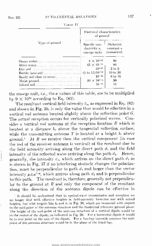
SEC. 25] FUNDA.If ENT AL RELATIONS 137
'I'ABLE 1V
Type of ground
Electrical characteristics of ground
Specific con- Dielectric ductivity e, constant K
em -cgs units (numerical)
Ocean water River water Dry soil Fertile farm soil Sandy soil close to ocean Moist ground Inland soil
4 X 10-11 80 45 X 10-15 80
10-16 3 to 5
(5 to 15)10-14 10 to 30 10-1s 8 to lo
30 X 10-'4 30 10-13 15
the em -cgs unit, i.e., the v values of this table, are to be multiplied by 9 X 10²° according to Eq. (83).
The resultant vertical field intensity 8z, as expressed in Eq. (82)
and shown in Fig. 36, is only the value that would be effective in a
vertical rod antenna located slightly above the reflection point G.
The actual reception occurs for vertically polarized waves. Con- sider a vertical rod antenna at the reception location R which is
located at a distance h,. above the tangential reflection surface, while the transmitting antenna T is located at a height h, above ground.' At R we receive then the vertical component (in case
the rod of the receiver antenna is vertical) of the resultant due to the field intensity arriving along the direct path dl and the field
intensity of the reflected wave arriving along the path d3. Hence, generally, the intensity g1, which arrives on the direct path d, as is shown in Fig. 37 if no interfering obstacle changes the polariza- tion, must be perpendicular to path d1 and larger than the vector intensity prs1e- i', which arrives along path d3 and is perpendicular to this path. The resultant is, therefore, generally not perpendicu- lar to the ground at R and only the component of the resultant along the direction of the antenna dipole can be effective in
1 It should be understood that in optical -wave transmission and reception we
no longer deal with effective heights in field- intensity formulas nor with actual heights, but with heights like h, and h, in Fig. 36, which are measured with respect to the mid -point of the antenna structure and the tangential reference ground plane. The height of the mid -point of the antenna structure of a vertical dipole would be to the center of the dipole, as indicated in Fig. 36. For a horizontal dipole it would be to any point on the axis of the dipole. For a five -bay turnstile antenna the mid- point of the antenna structure would he in the plane of the third bay.
www.americanradiohistory.com

138 FREQUENCY MODULATION [CHAP. I
producing a current in the antenna. If the rod antenna were turned parallel to the direction of the resultant, then the full available field intensity would be operative on the received current value. The same thing is true when the resultant field near the reflection point G is being measured with a rod antenna. Here, generally, the resultant (Fig. 36) of 82 and 83 has a slight forward tilt and for maximum receiver effects the rod antenna has to be tilted also and until it is aligned parallel to the resultant vector of 82 + 83. With respect to Fig. 37 and the reception location R,
Resultant vector El [I tpv B -1d.7at R j6
PvEic E
,90' 90°
Gov reflect/On factor for vertically polarized e. m. waves
Tangential plane
FIG. 37.- Transmission for curved earth. (Tangential plane Ti -G - R, used as fic- titious ground plane.)
we have to bear in mind that the direct and indirect field intensities have a phase difference that is due to two entirely different causes. One cause is the path difference d4 = (d2 + d3) - dl producing, according to Fig. 36, a phase delay S = 360d4/Á deg. This phase difference is taken care of by the factor e i3 in the expression for the indirect component field vector (Fig. 37). The other cause is the phase angle of the reflection coefficient Pv and is, therefore, contained in the expression for pv. We have for the resultant field 8r at R and the vertical reflection coefficient pv, the formulas
8r = c1(1 + Pve- ?s)
pK, -q (85) Pv - pece +q
where q vice -1+p2 p = sin 1,G
S = 360 d4
deg.
For horizontally polarized waves we have the corresponding
(86)
www.americanradiohistory.com

SEC. 25] FUNDAMENTAL RELATIONS 139
formulas r = g1(1 + PhÉ ia)
- Ph p+q (87)
if ph denotes the reflection coefficient for horizontal polarization. We note that the ground properties play a great part in determin- ing the effective electromagnetic field at R.
The effective dielectric constant Ke of Eq. (84) gives a means of finding from known numerical values for K and o- to what extent the ground is transparent to electromagnetic waves in the fre- quency range of the FM waves. If, for instance, the j term with the specific conductivity o- and the carrier frequency F is negligible in comparison with the K term, then the index of electromagnetic refraction n is equal to -\/-1-c and the ground may be considered a perfectly transparent dielectric. This was approximately the case for the numerical example given in connection with Eq. (84). Since this equation has the form Ke = a - jb, it gives directly the phase' of the reflection coefficient and we have C = tan-' (- b /a). For j terms very small in comparison with the real a term, which make Ke essentially equal to K, i.e., make the ground essentially transparent, no wave energy can be absorbed in the ground. The incident electromagnetic wave then is reflected toward the receiver with no decrease in amplitude and with a phase of the reflection coefficient that is either zero or 180 deg.
Suppose that we take a numerical case for which the imaginary term is 10 per cent or less of the actual K value in Eq. (84). Let us consider the case from Table IV for fertile farm soil having a
dielectric constant K = 25 and v = 5 X 10 -" em -cgs units for a carrier frequency of F = 49.9 Mc. We have, then, K, essentially equal to 25. In Eq. (86) we find that q is very nearly equal to 5,
since p2 under no condition can reach a value more than unity, as unity is also the upper limit for p. From Eqs. (85) and (87) we find the respective reflection coefficients
sin 1,1. - 5
/sin 1,G + 5 for horizontally polarized waves
P= 5 sin i' - 5
5 sin t,/i + 5 for vertically polarized waves
www.americanradiohistory.com

140 FREQUENCY MODULATION [CifIAY. I
Now suppose that the angle of incidence 1,G with respect to the tangential plane in Fig. 37 is 15 deg. Then sin ' = 0.2588 and we find for the horizontal polarization ph = -4.7412/5.2588 = -0.901 and for the vertical polarization p _ -3.706/6.294 = - 0.589. Hence, for vertically polarized waves, the reflected wave is considerably reduced in amplitude. Using all terms under the square root in determining the value of q, we find from Eq. (86) that q = X24.067 = 4.92, instead of the approximation 5, and that ph = -4.6612/5.1788 = - 0.901, which is exactly the value found with the approximation. The exact evaluation PU = - 3.626/6.214 = -0.584 shows also that for the vertical polarization the approximation yielding the value of - 0.589 seems close enough. We note that in each case we have a reflected wave which on account of the minus sign is 180 deg out of phase due to the reflection coefficient, besides the additional phase shift due to the difference distance d4.
Generally, it may be said that for horizontal polarization we may expect at G essentially 100 per cent reflection with a phase change of 180 deg in the frequency band used for FM work. This is also true for vertically polarized waves when the angle of inci- dence i' does not exceed 0.5 deg for reflections over land or river water. However, such assumptions cannot be made for reflec- tions over ocean water since then the conductivity is altogether too high. This explains why horizontally polarized waves for aerials located well above ground give better signal -to -noise ratios, than vertically polarized waves.
Since for small grazing angles both polarizations are subject to ideal reflections with a phase shift of 180 deg, we can now derive the radiation formula. In empty space the electric field intensity s in volts per meter for a dipole of effective height (effective length) he meters, at a distance d meters from the dipole, and for a current I amp, is given by the relation 8 = 185he1 cos v /(Xd). The operating wave length X is likewise in meters and v is the angle that the propagation direction makes with the equatorial plane of the dipole. If we use a half- wave -length rod as the transmitter aerial, we have an effective length of he = 0.3185X since for an actual length h of the dipole we have he = 2h /ir and h = 0.5X.
At the mid -point of the dipole where current value I is active, we have a radiation resistance of about 74 ohms with a radiated power of P = 7412 watts. Hence, in the foregoing formula
www.americanradiohistory.com
SEC. 25] FUNDAMENTAL RELATIONS 141
I = -VP/8.6 and we find
8 = 185 X 0.3185X A/P /(8.6Xd) = 6.85 -05/d volts /meter
This is the field intensity in the equatorial plane of a half -wave dipole or rod antenna at a distance d meters for a radiated power of P watts. By equatorial plane is meant the plane through the mid -point of the rod and perpendicular to the rod.
This formula applies to both the direct and the indirect path of the system shown in Fig. 36a. For the indirect path trans- mission, phase and reflection effects must also be considered. The phase delay due to the path difference d4 is S = 27rd4 /X,
where in the formulas for d2 + d3 and d1 the value of d2 is large
compared with the values of (ht + hr)2 and (ht - hr)2. There- fore, we may use the approximations d2 + d3 = d + 0.5(ht + hr)2 /d and d1 = d + 0.5(ht - hr)2 /d. Hence, d4 = d2 + d3 - d1
2hthr /d with a corresponding phase delay S = 4irhthr /Xd. This is the phase delay at R for the indirect wave with respect to the direct wave with propagation over plane ground and gen-
erally for small grazing angles and holding for either type of
polarization. According to the numerical outcome of Eqs. (85)
and (87), for horizontally polarized waves we have the reflection coefficient ph essentially equal to -1 and the resultant field inten- sity at R is
sr= 81(1 -C-i)= (1- cos y +j sin 5)81 =m81
But the phase delay S = 720hthr /(Xd) = 720p deg. can, on
account of the very small value of p due to the large value of d in
comparison with the relatively small value of the product of hthr,
correspond only to values of S not exceeding about 11 deg. For such angles cos S is essentially equal to unity and sin 5 is equal to 471-hthr/(ad) = S. Hence,
sr = 81(1 + jS) = 815 -V1 + 52
since the phase angle is tari 1 5 and, on account of its smallness, is equal to S radians. Hence, for horizontal polarization, on
account of -V1 + 52 being practically equal to unity, we have sr = 815. But according to the above derivations, we have for a
half -wave sender antenna 81 = 6.85 -P /d and, therefore,
8r 6.854 VP - 86.1 hthr VP
(88)
www.americanradiohistory.com

142 FREQUENCY MODULATION [CHAP. I
The electric field intensity 8,. at the receiver R is in volts per meter, and the respective heights ht and hr, as well as the operating wave length X and distance d, are in meters. Since Eq. (88) was derived for horizontally polarized waves, it is assumed that the transmitter dipole or half -wave rod is placed horizontally. Theoretically, a similar horizontal dipole facing broadside to the transmitter half - wave rod should give maximum reception effects and give a field intensity in accordance with Eq. (88). Since in FM transmitters turnstiles are usually employed, the field intensity received is G87. where G denotes the gain produced by the transmitter antenna over the field radiated by a single horizontal half -wave dipole.
Since d meters are equivalent to d/1,609 miles, h meters equal to 3.281h ft, g volts /m = 106ßµ volts /m, and X meters equivalent to (300 m /sec) /(F Mc /sec), we have the comparison formulas
F hth r -VP 0.0103 for FM frequency allocations
(89) 4,257 P
for customary standard broadcast allocations
In each case half -wave radiators are used, the radiated power P is in watts, the respective heights ht and hr in feet, the distance d in miles, and the carrier frequency F in megacycles. It should be understood that these formulas have nothing to do with the type of modulation or type of signal current, except that the upper formula applies to the carrier -frequency range used for the FM frequency allocations mentioned at the beginning of this section. A tele- vision signal, or any AM signal using frequencies F of this range (around 50 Mc), gives field intensities at R in accordance with the upper formula; for the standard broadcast frequencies, the lower formula holds. What is of importance is the fact that for the FM range of carrier frequencies the field intensity decreases with the square of the distance, instead of only inversely with the distance. Generally, we can write the lower formula as k s15/d, if the ground absorption is not taken into account. The factor k depends partly on the effective height he of the antenna system. If this expression is compared with k1F /P /d2 which represents the upper formula of Eq. (89), we see that here k1 depends on the actual elevations ht and he above the tangential plane through the point G of reflection (Fig. 38). The field intensity is also propor-
www.americanradiohistory.com

SEC. 25] FUNDAMENTAL RELATIONS 143
tional to the carrier frequency F, which indicates an advantage for the higher carrier- frequency allocations in the FM range.
For the standard broadcast frequency assignments, the carrier frequency, even though not seen in the lower expression of Eq. (89),
is indirectly effective on the value of sr. For daytime reception we have to deal mostly with the ground wave for which the
T
(Q)
Er measured fie /d in ,a v/m
R
r
d miles
Path difference d4 = d2 td3 -d,
Effective free e,uv /m _4.13243x108d2Er
space field ° hthrF
Fin Mc, ht and hr in feet and din mi /es
(b)
Er
d mi/es FIG. 38. -How the heights h, and h, in field- intensity formulas can be found.
Sommerfeldian numerical distance plays a part. This numerical distance is effective in determining the attenuation or absorption factor by which gr is to be multiplied. This factor has smaller values for the higher carrier frequencies in the standard broadcast range. Hence, the very opposite happens in this range as far as the variation of propagation with the carrier frequency F is
concerned. The upper formula of Eq. (89) holds very well for horizontally
polarized waves, even applying also to vertically polarized waves for small grazing angles if the point of reflection does not happen to be located on a fairly good conducting surface such as, for
www.americanradiohistory.com

144 FREQUENCY MODULATION [CHAP. I
instance, ocean water. For such a surface at the point of reflec- tion, the ground is no longer dielectrically transparent, i.e., free of losses, and the reflected wave is returned not only with most any phase angle instead of with a phase reversal, but also with a greatly diminished amplitude. For all such cases we can write down expressions that can be used for computations by means of Eqs. (85), (86), and (87). We then have, since p2 = sine 4 cannot be very large in comparison with customary values of Ke
in Eq. (86), for line -of -sight distances that are large compared with the respective elevations IN and hr (as is usually the case when we are several miles from the transmitter station), the approxima- tion q = - 1 and the formulas
r =
Ke Sin tÿ - 'Vice - 1 ) for vertically / e--)8
Ke sin 1/ + -Vice - 1 polarized waves
sin 4/ - V Ke - 1 _;al E /
for horizontally
sin 4/ + V Ke - 1 polarized waves
(90)
for S = 4irhthr /(Ad) where h,, hr, X, and d must be expressed in the same dimensions. Hence, we may again expect higher resultant field intensities for horizontal polarization. According to Fig. 36 sin 4, = (ht + hr) /(d2 + d3) which for d large in comparison to h, and hr yields the approximation sin 1,G = (h, + hr) /d = t'/. We have, then, for the respective reflection coefficients
4 -VKe- 12(h.t +hr) -= 1 Ph
1 J
E l S
}
;bl f
horizontal
vertical
(91)
(92)
(93)
1,1/ + Ke -1 d-V
P - Ke -1
+ hr) ll/Ke - -V Ke - 1 2Ke(ht
II/Ke + \V Ke - 1 d
Therefore, for horizontal polarization
r =1 1
and for vertical polarization
gr 81 { 1 +
V Ke - 1
[2(ht + hr) - d VKe - 1
[2Ke(ht + hr)] dVKe - 1
These formulas can be readily evaluated in numerical cases.
www.americanradiohistory.com

SEC. 251 FUNDAMENTAL RELATIONS 145
As to the formulas given, note that we have to use the heights ht and hr, which are expressed in feet in Eq. (89). Generally, we are confronted with wave propagation paths as indicated in Fig. 37. As far as the line -of -sight distance dl of the direct path and the two propagation portions d2 and d3 of the indirect transmission path are concerned, we have exactly the same triangulation as in Fig. 36, where plane earth was assumed. The only difference is that the tangential plane represented by the line T1GR1 in Fig. 37 is substituted for the plane ground with only point G in the actual ground. Even though the normal primary service radius is not great for such high carrier frequencies as are used for FM, we still should not neglect the curvature of the earth. We should also realize that we have a certain amount of electromagnetic refraction in the earth's atmosphere close to ground for such short waves. This refraction is usually taken into account by still taking the propagation paths straight, but assuming an equivalent radius of the earth which is about 33 per cent larger than the actual radius.
With this in mind we see that we have actually only three distances that we know in Fig. 37: the height TT2, the height RR2, and the curved distance T2GR2. At first we know nothing about the exact location of the earth point G in the hypothetical reference plane indicated by T1GR1. The distance TT1 is then the distance from the hypothetical reference ground plane at the transmitter to the mid -point of the actual transmitter antenna structure. For a simple horizontal half -wave antenna it would be the distance from the ground plane to the rod antenna. For a vertical dipole it would be the distance from the ground plane to the mid -point of the rod antenna. For a five -bay turnstile it would be the dis- tance from the ground plane to the plane of the third bay. It does not matter whether it is the third bay from the top or from the bottom of the turnstile, since with an odd number of bays it will be always the same plane, as in this case it is always the third bay plane. For an even number of bays, say six, the point T is 3 bay planes up from the bottom of the turnstile or 3 bay planes down from the top.
In Eq. (89) and the other corresponding Eqs. (92) and (93), we require the heights ht and hr of Fig. 37. Hence, we have to find first the point G. This is readily done since the angle of
incidence 4 must be equal to the angle of reflection 4/ and points
www.americanradiohistory.com

146 FREQUENCY MODULATION [CHAP. I
T and R are known. When, as is usually the case, the path difference d4 is smaller than one -sixth of the operating wave length, we have, for the respective dimensions used in Eq. (89), for the path delay due to d4 a value S = hthrF /d < 433 X 103. From the distances GT2 and GR2 in miles, we find the heights T1T2 and R1R2 in feet from the relations T1T2 = 0.5071 and R1R2 = 0.5GR2. These formulas account for the curvature of the earth's surface and for the small downward atmospheric refraction, which causes a slightly longer propagation path than indicated by the line -of- sight distance. Hence, the required heights ht and hr can be computed from the formulas
ht = TT2 - 0.5G711 (94)
hr = RR2 - 0.5GR2
where ht, hr, TT2, and RR2 are in feet and GT2 and GR2 are in miles. Equations (89), (90), (92), and (93) assume ideal unobstructed
wave propagation conditions; i.e., only the one reflection at the ground point G occurs. For this reason the FCC requires that the values of the free -space field intensity go of Fig. 38 be found from computations based on actual measurements of the effective field intensity at a distance of several miles from the transmitter in different directions and within the line -of -sight distance. The procedure, as well as the formula in this figure, holds only for waves having horizontal polarization where >li is a small angle (almost grazing angle of incidence). This procedure would not be reliable for the case of vertically polarized waves.
It should be realized that for hilly ground contours in certain directions of the transmitter T toward a reception point R, there may be several ground points where electromagnetic reflections toward R are possible. It is, however, the path triangle for which the path difference d4 has a minimum value that counts, since this minimum path will cause the largest effective field intensity 8r
at the reception location R. The stipulation of a minimum value for d4 for given locations T and R will also result in the smallest product value of hthr. In Fig. 38 two cases are indicated using a five -bay turnstile transmitter aerial in order to produce, at least theoretically, a horizontal circular radiation pattern in the equa- torial plane through the third bay or crossed dipoles. Figure 38a then depicts the most common arrangement where the reception point R, with a resultant field intensity sr, is so located that h,.
www.americanradiohistory.com

SEC. 25] FUNDAMENTAL RELATIONS 1.17
is essentially equal to the true elevation of the receiving horizontal dipole above ground. The dipole is perpendicular to the TR direc- tion. In Fig. 38b it will be noted that the most suitable trans- mission path triangle requires at the receiver location R a height h, which is many times larger than the actual elevation of the receiv- ing dipole above ground. The ground elevations above normal sea level are drawn with an exaggerated elevation scale in these figures, which means that the line -of- sight distance d1 is drawn way out of proportion and altogether too small with respect to the elevation scale. For this reason the angles 4' and >!i, cannot always he shown as equal for such exaggerated elevation scales. The paths d2 and d3 should, therefore, he drawn in such a manner that the respective heights h, and hr come out proportional to their horizontal distances from the point G where the ground reflection takes place. In this arrangement IN and h,. are measured vertically rather than perpendicularly to ground, as in Fig. 37.
Figure 39 is presented here with the kind permission of the engineering department of the FCC and is helpful in computing field intensity contours. For these curves, the power P is in kilowatts, G expresses the transmitter antenna field gain, and 8
denotes the desired field intensity in microvolts per meter. For example, the field intensity 8 has a value of 50 for the 50µv /m con- tour. The quantity h stands for the transmitter antenna height h, in feet, and r = 50hG 1/8. With respect to field gain, reference is made to page 149. In connection with Fig. 39 we compute first the value of r from the inscribed formula. Then, from Fig. 39 we find the distance d in miles for the calculated value of r, from the point of intersection of a vertical with the appropriate power curve.
Suppose we have a 30 -ft receiving antenna and a transmitting antenna height of 750 ft and want to determine the distance in miles to the 50 µv,'m contour for an FM station in the 42- to 50-Mc band. Suppose that the antenna power is 500 watts, and the antenna array is such that we have a field gain of 2. We must, on account of the square -root law of the upper relation of Eq. (89), multiply the true antenna power of 500 watts by 22 in order to obtain the effective power that causes 6. We obtain 4 X 500 = 2,000, which means that the effective value of P = 2kw. The distance to the 50 µv /m contour is found by estimating in Fig. 39 the 750 -ft curve. It is halfway between the 500 -ft and the 1,000 -ft
www.americanradiohistory.com

148 FREQUENCY MODULATION [CHAP. 1
curves. We then find the intersection of the horizontal line through the 750 -ft ordinate with the 2 -kw 45 -deg line belonging to the 50 µv j m contour. We proceed then vertically- downward
Ó U Ó 0 ó CS
\ \:\ \\,\ \\ \ \\\. \ \ \ \\
O Ó Ó ó o C ó G i
- - o n d m .+i
.v N - -
1333 NI 1H913H VNN3INV 9N111IWSNVa1 2:10 S31111 NI 39NV1Si0
in order to find the intersection with the 750 -ft curve. Tite height of this intersection point read off on the distance scale
then gives the ronge in miles and is in titis particular cose equal
to 54.5 miles. If this procedure is reversed, Fig. 39 cari be used
www.americanradiohistory.com

SEC. 25] FUNDAMENTAL RELATIONS 149
for finding the power required for a given antenna height in order to cover a certain distance with a 50 tv /m level. It will be noted that these curves also enable us to make calculations for the 1,000 µv /m as well as for the 5 ,uv /m contours.
Moreover, with respect to the upper field intensity formula of Eq. (89), we have to remember that it is based on a half -wave dipole transmitter antenna. However, like the above, it is directly applicable to other antenna arrays when the field gain is
known. Some manufacturers give the field gain and others give the power gain for their antennas. If the field gain is given, the factor is to be squared and multiplied by the true power value in order to obtain the effective value for P to be used under the square -root sign. If the power gain is given, the factor is to be directly multiplied by the true power rating in order to obtain the value for P to be used under the square -root sign. H. H. Beverage and M. G. Crosby' have extended the radiation formula in the ultrahigh- frequency range to distances beyond the horizon. The distancez dh to the horizon in miles for the heights hr and h, in feet is given by the formula
dh = 1.22(ha -f N/h,.) miles (95)
The upper formula of Eq. (89) is then
= 0.0103 hrhrdhd1F P
uv /m (96)
where d is the distance in miles from transmitter antenna located ht ft above the tangential plane to the receiver antenna of height hr ft with respect to the tangential plane. The quantity dh is the distance in miles from transmitter to the horizon, F is the carrier frequency in megacycles, and P is the effective wattage; i.e., the actual power in the antenna times the antenna power gain over one half -wave dipole. For a half -wave antenna at the transmitter, P will be equal to the true antenna power. If the distance d to the receiving antenna is smaller than the distance dh to the horizon, then the exponent q is equal to 2 and the semiempirical formula (96) degenerates into Eq. (89). For present -day FM frequency allocations, we have q equal to about 3.5. This value is the out- come of experimental determinations.
BEVERAGE, H. H., RCA Rev., 1, January, 1937. CROSBY, M. G., RCA Rev., 4, 349, 1940.
2 For other details, consult "Phenomena in High -frequency Systems," p. 362.
www.americanradiohistory.com

CHAPTER II
AUXILIARY APPARATUS EMPLOYED IN FM SYSTEMS
Since frequency modulation is based on variations along the time axis of a current wave, we need not only devices for producing such effects but also devices for extracting signals at the receiver end. We also have to use apparatus for removing undesirable AM effects, which may be inherent to certain methods of producing FM or may be due to interference. As complicated as the produc- tion of an FM current may seem, it can be done at low power rating, i.e., with tubes that are used in receiver engineering. Frequency multiplication is accomplished after the primary or "master" FM has been brought about and the final stages involve mere step -ups in power.
It should be realized that amplification of power in FM systems can be done efficiently with ordinary power amplifiers since the current level remains constant. This is a great inherent advan- tage with this type of modulation as compared with amplitude modulation.
26. Balanced Modulators. -Balanced modulators can be used for producing the amplitude modulation product, i.e., the com- pletely modulated portion of a carrier current. It is, then, the portion b in Eq. (2). The portion a, which is of carrier frequency F, is automatically suppressed.
The reason for suppressing the remaining unmodulated carrier component is that the modulation product can then be shifted in phase and, as is shown in Fig. 3, can be added geometrically with the a component in order to produce another type of modulation. We have then generally PM + AM.
One way of removing the carrier -frequency component of an AM wave is by "bucking" out the carrier component at the output side of an amplitude modulator. This is done by means of an induced voltage, which causes a current flow ( -)Im sin Sgt in opposite direction to the component a = ( +)Im sin SZt. This is comparatively easy to do since the a component has the original I,,, level for any degree of AM and is of pure sine shape.
150
www.americanradiohistory.com

SEC. 26] AUXILIARY APPARATUS 151
Superior methods for the elimination of the carrier component are the bridge and differential methods, since they are based on balance and will inherently cancel out the carrier -frequency component. A modified Wheatstone bridge circuit can be used. One branch of the bridge forms a series inductance -capacitance combination and is tuned to the carrier frequency F. The ohmic resistances of the other three branches are made equal to the effective resistance of the tuned branch. Hence, if the output
Modulation 6-- frequency f input o
Fand f input
Carrier frequency F
input
Out F2F,2f; JF ;(F ±2f
Side band output
f; (Ftf), (2F ±f); Jf
F; f; 3F; (2Ftf); (F2'2f)
Side band output
2F; 2f; (Ftf) 40.- Balanced modulators.
voltage of an amplitude modulator is applied to any two diagonal bridge points, a load connected to the other two bridge points can experience only currents that are not of the frequency F for which the bridge is balanced.
Much more convenient are balanced tube circuits, such as are shown in Fig. 40. These circuits, well known in the art, are self - explanatory. The side -band output terminals are marked in this figure. It is the upper network that is of greatest use, since the signal voltage and the carrier voltage are applied through separate transformers and in such a way that no power transfer is possible between the carrier -frequency and the signal- frequency sources. For the upper network the signal voltage em cos wt acts in push -pull on the two grids while the carrier voltage Em sin Sgt
www.americanradiohistory.com

152 FREQUENCY MODULATION [CHAP. II
acts in equal pull on these grids. Hence, when the voltage Em sin Sgt + em cos wt is effective on one grid, we have a voltage Em sin Sgt - em cos wt acting on the other grid, say on the lower one. The upper grid experiences, therefore, the amplitude effect of Em(1 + K cos wt) where K = em /Em and the lower grid experiences the amplitude effect Em(1 -K cos wt). The current variation in the upper tube is, therefore,
Im sin Qt + 0.5KIm[sin (Q + w)t + sin (12 - w)t];
for the lower tube we have
Im sin Qt - 0.5KIm[sin (Q + w)t + sin (Q - w)t].
But as far as the secondaries of the respective plate transformers are concerned, these current variations act in opposition and we have the effects
+Im sin Sgt + 0.5KIm sin (Q + w)t + 0.5KIm sin (0 - co)t
-Im sin Qt + 0.5KIm sin (Q + w)t + 0.5KIm sin (Q - co)t
which, added together, show that KIm[sin (Q + w)t + sin (Q - w)t]
remains. (2KIm cos wt) sin Qt, the corresponding modulation product, is the only component that is effective in the output current. This modulation product has twice the amplitude value of the corresponding product in Eq. (2). This should not matter since this amplitude difference is due only to a constant of propor- tionality like the fixed mutual inductances that are instrumental in causing the output current of the modulation product in the secondaries of the plate transformers.
In FM systems we use, besicles, balanced transformers, which cause balanced reactance injections as far as the steady reactance component is concerned. This is discussed in the sections dealing with reactance modulators.
27. Ring Modulators. -Ring modulators are important since they are used in connection with frequency division (consult pages 154, 242). Figure 41a shows a ring modulator, which is
likewise a balanced modulator and produces only the modulation product; i.e., it suppresses the carrier -frequency component. Since contact rectifiers are often used for the rectifiers 1, 2, 3, and 4 in Fig. 41a, such as the well -known cuprox dry -disk rectifier, the suitable type depending on the frequency range, there is also indicated in Fig. 41b the rectifier bridge circuit employed in
www.americanradiohistory.com

SEC. 27] AUXILIARY APPARATUS 153
alternating- current instruments in order to clear up any confusion that may arise about the differences between these two circuits. In the amplitude modulator network of Fig. 41a, the rectifiers are connected all in direct series, so to speak, "around a ring." A direct- current flow is then possible from A to C to B to D and back to A. In the rectifier connection of Fig. 41b, the polarity of the rectifiers 1 and 2 must be such that direct -current flow toward point C is possible, just as rectifiers 3 and 4 must also permit the return flow of the current I, + I. Hence, when an
4-112
E,,,sinitt
e,,,cos wt
Load
Hernating, current
(a) BALANCED RING MODULATOR
FIG. 41.- Connection and action of the ring modulator.
Direct current indicator
(b)
Load
(c)
alternating voltage is applied to points A and B, a direct- current meter will experience a corresponding unidirectional deflection.
It is, of course, the ring modulator that concerns us. The connections of Fig. 41a bring about AM in the load branch if a carrier voltage Em sin (6.28F)t and a signal voltage em sin (6.28f)t are applied as indicated. What happens in case of an abrupt or "keying- fashion" modulation instead of a smooth AM can be readily understood from Fig. 41c. Here a switch is used in place of the "electric- bridge" switch effective in Fig. 41a. Suppose that in Fig. 41c the reversing switch reverses the polarity of the applied voltage E2 of carrier frequency F many times, say f times per second; then the voltage E3, which is effective across the load, will key or modulate the current coming from the F source. Exactly the same thing will happen in Fig. 41a except that the keying is not abrupt but is according to the em, cos wt law. During the positive half cycle of the signal current of frequency f, the
www.americanradiohistory.com

] 54 FREQUENCY MODULATION [CHAP. II
bridge point A will be positive with respect to the bridge point B and the voltage 2E1 produces a direct -current flow in accordance with the time function cos wt. During such a current flow, G is electrically connected with C so that the carrier -frequency source of voltage E2 applies a voltage E3 across C and H. When wt is 90, 270, etc., deg, then 2E1 is zero and bridge points A and B are equipotential; hence, no carrier current can flow toward the load. But, when the voltage 2E1 passes through its negative cycle, the rectifiers 3 and 4 permit a direct -current flow since bridge point B is now positive with respect to bridge point A. Therefore, the
FIG. 42.- Frequency division by regenerative modulation.
carrier voltage E2 is effective again and causes the corresponding voltage E3 across H and D but with reversed polarity. Hence, the current of signal frequency f modulates the carrier current of frequency F with the carrier component of frequency F suppressed.
28. Frequency Division by Regenerative Modulation. Figure 42_ shows an application of a ring modulator for dividing the carrier frequency by means of regenerative modulation. As far as the modulation action is concerned, it is exactly the same as in Fig. 41a except that the current of frequency f is the outcome of the current of frequency F and bears a subharmonic relation to the F current. Suppose that a 10 -kc voltage is applied across ter- minals a and b. The plate circuit of the tube is tuned to half the frequency for this particular numerical case, i.e., to 5 kc. This 5 -kc output is fed back by means of the secondary voltage produced across e and g to points k and h, thus causing a keying or modula- tion action which is at the same time in half- frequency step with the current to be modillated. The resulting output across ter- minals c and d is, therefore, a current of frequency which is only 5 kc.
www.americanradiohistory.com

SEC. 29] AUXILIARY APPARATUS 155
Figure 43 shows a case where by means of two ring modulators, I and II, and only one tube, successive frequency halving is accomplished; i.e., a final frequency equal to one -fourth of the original carrier frequency is obtained. Suppose a 10 -kc voltage is again applied to the ring modulator I and the upper output tank is tuned to half the frequency value, i.e., to 5 kc. A portion of the tank energy is fed back toward the other diagonal bridge point of the ring modulator I in order to cause modulation. The other
2 FIG. 43.- Cascaded frequency division employing two -ring modulators I and II and one
and the same tube for regenerative modulation.
Tuned toSkc I
Tuned to
2.5kc
Goes fi input '
kc of e=./g
2 modu/aforll 0 Back-feed of Sfro-current
c
rZSkc-ouf
d Co
Back -feed of2.Skc- current
secondary of the 5 -kc tank applies its terminal voltage across 1
and 2 to ring modulator II. The corresponding lower tank of the external plate circuit is tuned to 2.5 kc and a portion of the tank energy is fed back to the other diagonal bridge points in order to cause electric keying. Hence, at the output c -d a 2.5 -kc current is finally obtained.
29. Reactance Tubes. -Reactance tubes have the object of injecting reactances into associated networks. If the associated network is an ordinary tube oscillator whose frequency is not stabilized, i.e., "not stiff," then the reflected reactance will change the frequency of the oscillations that are generated. But if the frequency is stabilized, i.e., "F is stiff," as in a piezo oscillator or in a carrier -frequency amplifier without sufficient back action, then the injected reactance will cause a corresponding phase shift. Hence, when the injected reactance swings or varies, FM will be caused in the former case and PM in the latter case.
www.americanradiohistory.com

156 FREQUENCY MODULATION [CHAP. II
The case of FM is of importance since some commercial FM transmitters are based on such modulators and considerable frequency deviations can be caused directly by this method. Fig- ure 44a shows a reactance or quadrature tube Tm which, with its plate load R1C1, causes reactance fluctuations in the oscillator frequency- determining CL branch, which is the plate load of the
Reactance tube tor Oscillator High modulator 1-( To. frequency ______ C3 1 C4 choke
+8
Cs _CI
C L
E!
R2 4
emsm cot
g Fired negative grid bias
1
XfdXsin cot H C
(a) Note: The smaller the injected
reactance the more change in the oscillator frequency
E
2 !p t!
(b)- Equivalent oscillator and modulator network FIG. 44.- Action of reactance modulation.
oscillator tube To. From the equivalent network of Fig. 44b
we note that a reactance X + OX sin wt is generally injected across terminals 1 and 2 of the frequency- determining network of the actual oscillator. The portion X represents the steady or fixed reactance and the portion AX sin wt represents the variable reactance component applied to 1 -2. It is the variable component OX sin wt that brings about FM. The fixed component X is also used in FM systems, but for stabilizing the center frequency of the master oscillator. The fixed reactance X is affected by the fixed negative -grid bias of the modulator tube Tm. This bias determines about which reference mutual conductance value the variations in the dynamic mutual conductance due to the signal voltage em sin wt take place.
www.americanradiohistory.com

SEC. 29] AUXILIARY APPARATUS 157
Now any tube oscillator sustains oscillations on account of the energy fed back from the plate circuit into the grid circuit, which, in turn, due to the amplification property of the tube, causes the maintenance of the plate current variation. Hence, the feedback into the grid branch and the subsequent "through- grip" within the tube due to its grid -into -plate actions must be such that the plate current oscillations remain fixed not only in amplitude but also in phase. The latter is often overlooked since for ampli- tude modulation the phase does not matter and for customary a -f amplifications we have no perceptions as far as our ear is concerned when phase distortion occurs. The amplitude balance in an oscillator satisfies the energy balance requirement and the second condition satisfies the phase balance requirement. If, for instance, the energy balance requirement is not met, we should experience some sort of AM. What would occur in one case is that for subsequent grid -into -plate actions more variable plate current would be produced. Then the amplitude of the plate current would keep growing until the plate- current saturation limits the action, or until the increase in circuit losses just prevents a further amplitude growth. For the other case, if the energy due to the internal "through- grip" of the tube is not sufficient to supply the circuit losses, successive amplitudes in the plate - current variations will decrease until the oscillation stops alto- gether. Neither of these cases concerns us here. The only condition of interest, namely, that for growing oscillations, on account of ultimate energy balance or on account of plate - current saturation, whichever might be the case, would cause sustained oscillations in next to no time. But the inphase requirement is important since it can be used for causing useful PM as well as useful FM. Thus if, for instance, the subse- quent plate -current variations during a certain period of time are advanced in phase with respect to the plate -current variations that are affecting the grid potential of the oscillator tube by feedback action, then the frequency of oscillation cannot remain constant since each following cycle speeds up somewhat more than the pre- ceding cycle. In the same way, if the subsequent plate -current variations are lagging in phase, then the corresponding oscillation frequency must gradually drift to lower values. It is this unde- sirable feature in any ordinary tube oscillator which is made use of in reactance modulators. It is generally not done by a feedback
www.americanradiohistory.com

158 FREQUENCY MODULATION [CHAP. II
within the oscillator, but in virtue of an injected out -of -phase current coming from an associated network. The associated network is known as the output branch of a reactance tube.
In Fig. 44a condensers C3 and C4 are coupling elements and condensers C2, C5, and C6 are by -pass or isolation condensers. They can have, therefore, no frequency effect as long as their magnitudes are properly chosen. Condenser C4 acts as a feedback coupling condenser toward the oscillator grid; condenser C2 acts as a forward coupling condenser toward the control grid of the modulator tube Tm. The modulation action that takes place in the circuits of Fig. 44 is, then, as follows:
The tank voltage E across points 1 and 2 causes a correspond- ing current flow in the series combination of resistance R1 and capacitance C1. If R1 is chosen at least five times the value of 1/6.28FC1, then this current can be considered as essentially in phase with the driving tank voltage E. Hence, I1 is vertical in Fig. 44c as is vector E. The voltage E1 across condenser C1 caused by this current I1, then lags II by 90 time degrees and is, therefore, in quadrature. Hence, it is drawn to the right in the vector diagram of Fig. 44c. Essentially this voltage E1 is applied to the control grid of the modulator tube Tm. It "triggers off" a cor- responding plate current variation ii,, which essentially flows only to points 1 and 2 and back toward the cathode of tube Tm, since R1 is high in comparison to the multiple reactance across points 1 and 2. Theoretically, this reactance would be infinite if parallel resonance could take place with no resistance effects. But in practice the parallel combination of C and L acts like an ohmic resistance which is much smaller than the R1 value and very much smaller than the impedance offered by both R1 and C1. The iP
current is in phase with the voltage E1 and causes, therefore, a superimposed current in the plate tank of tube To which lags 90 deg behind the original tank current. This is the reason why for a 90 -deg out -of -phase action, Tm can also be called a quadrature tube. Since we deal with a lagging current, the reactance across points 1 and 2 can no longer be infinite unless something happens. If I is the circulating tank current, what occurs is that the resultant current I -I- iP will change its original carrier frequency Fo to another value until the total reactance across points 1 and 2 is again infinite. But this means that in equivalence a corresponding
www.americanradiohistory.com

SEC. 29] AUXILIARY APPARATUS 159
reactance X has been injected in parallel with both the tank con- denser C and the tank inductance L.
This is exactly what happens when terminals 3-4 are shorted. Since the mutual conductance gm = ó2p /aEi, we note that the magnitude of the positive reactance X, which is injected across points 1 and 2, depends directly on the mutual conductance of
the operating point on the modulator tube characteristic. Hence, the value of X can be controlled by varying the negative grid bias of the modulator tube. Therefore, when a variable signal voltage em sin wt acts across terminals 3 and 4, the corresponding impressed reactance across terminals 1 and 2 is Xt = X + OX sin wt at any instant of time. If the voltage E1 had been taken off across the resistance R1 instead of across C1 and 1/(6.28FC1) ? 5R1, then the ip current reflected back into the oscillator tank circuit would have been a leading current. Hence, a negative reactance would have been impressed across terminals 1 and 2; i.e., a carrier - frequency increase would result as far as the steady component is
concerned. The action just discussed finds two important applications in
FM systems. One is that we have a modulator that gives a
means for translating signal voltages directly into corresponding carrier -frequency variations. The other application has to do with the steady component X in the value of X t. This component gives a means for correcting any slow frequency drifts in the center frequency F by applying an appropriate grid bias to the modu- lator tube. This is done in the RCA as well as in the General Electric Company's FM transmitters (consult pages 128 and 236), where a frequency discriminator is used for translating any slow frequency drifts into either positive or negative volt- ages when the correct center frequency F is either exceeded or fallen short of. These output voltages are then made to act in proper polarity in series with the fixed grid bias of the reactance tube modulator. This modulator brings about FM and the reactance tube will then automatically correct the desired center frequency F by reflecting the proper reactance into the tank circuit of the master oscillator, owing to the grid bias change.
It should also be understood that the reactance tube does not necessarily have to be a quadrature tube in order to cause FM. By quadrature tube is meant a modulator tube that injects pure
www.americanradiohistory.com

160 FREQUENCY MODULATION [CHAP. II
reactances due to plate currents ip that are exactly 90 deg out of phase with the driving tank voltage E. Any reflected current ip that is out of phase by an angle with respect to the phase of the tank voltage E will impress an impedance Z = R ± X across
Quadrature tube modulator
(b) CLASS-A MODULATOR
49m
Operating point
eInsinrolo-ó Eci
Erg ; T,,
High /a-tube such as a 6ÁG7 or its equivalent
>1-c- --Oscillator--
0E C I
I =110E
(a) DYNAMIC NETWORK
9max
-Cc I 0 gO
E level without
1 modu /a/ion
_/-! ,-r i
Out
g,,; variation
i
2 No
modulation
r
Eg Note that for such a modulator the time -axis swings
r em sin iul I
Time
Time
Injected current o =gm E, cos l! t +g,,, em sin w r
--Time
I-4- Modulation- - k- No
modulation FIG. 45.- Performance in a class A frequency modulator.
terminals 1 and 2 of Fig. 44, and will cause FM. This is, however, not desirable since the resistance component is apt to cause appreciable dissymmetry with respect to the center -frequency position when large variations are involved as in wide -band FM.
What occurs in the general case can be readily understood from Fig. 45a, where only the dynamic network without any steady
www.americanradiohistory.com

SEC. 29] AUXILIARY APPARATUS 161
supply voltages is shown. We note from this figure that the reactance tube' Tm is dynamically directly across the oscillator tank circuit and, therefore, is also in multiple with the oscillator tube To. By tube is meant, in each case, the plate -to- cathode path of the particular tube. Hence, for a lumped dynamic tube voltage ei = ei, - µee we have the corresponding dynamic plate current ip = ei/r, where a and r1, denote the dynamic amplifica- tion factor and the internal dynamic tube resistance, respectively, of the modulator tube T,n. It is really an internal tube impedance in this case instead of a dynamic tube resistance since ep /ip is, in the general case, an impedance with an active and a reactive component. Substituting m for e0 /e,,, we have
C 1 mµ\ ip = ep = Yep
rp rp
where Y = ip /ep is the admittance. It must also he complex and when expanded is
Y= 1 (1 - m,µ cos cp) -jmµ r -1 sincp =A - jB (97) rp
The real part vanishes for cos cp = 1 /(mµ). Hence, generally the plate -to- cathode path of the modulator tube Tm acts as though an admittance of amplitude value \/A2 + B2 with a phase tan-1 ( -B /A) were connected across the tank circuit of the oscillator. The corresponding complex impedance in shunt with the tank impedance determines the effective oscillator frequency Ft, since to circulating tank currents the total reactance must vanish in case of natural tube oscillations. When the real term A vanishes, we have only a reactance
AX - 3r, (98) mµ sin cp
injected in the frequency -determining branch of the oscillator circuit.
Generally, it may be said that for larger L/C ratios in the tank circuit, the AX effect and the corresponding frequency deviation AF in the center frequency F will be larger, but at the expense of
1 For the general case we deal with an impedance tube rather than with a quadrature tube or a reactance tube since i is no longer 90 deg behind or ahead of the driving tank voltage E.
www.americanradiohistory.com

162 FREQUENCY MODULATION [CHAP. II
less stable tube oscillations since for high L/C ratios the frequency stability is poorer. Equation (98) shows that AX is directly proportional to the dynamic plate resistance of the modulator tube Tm. Since low values of AX in parallel with the tank react- ance across terminals 1 and 2 give more AF deviation, a power reactance tube is desirable since a power tube has a low dynamic plate resistance.
30. Design Formulas and Useful Quadrature Tube Modulators. In Sec. 29 we learned that either a leading or a lagging current may be superimposed on the normal tank current. The tank circuit in Fig. 44a consists of a condenser in parallel with an inductance. It is correct to assume that, in equivalence, a superimposed cur- rent, due to the action of a reactance tube modulator that is 90 deg leading with respect to the original tank voltage E, causes more condenser current since the superimposed current is in phase with the original condenser current. Hence, the superimposed current must cause an equivalent increase OC in the value of the normal capacitance C. This will then account for the corresponding OF decrease and the new oscillation frequency F. In the same way, a 90 -deg lagging iP current is in phase with the normal current through the inductance L of the tank. This must cause an equivalent decrease AL in the normal value of L. This will then account for the increase in the oscillation frequency. It can also he assumed that a 90 -deg lagging ip current with respect to the normal tank voltage E, since the current is in antiphase with the normal C current, must cause a decrease 6.0 in C. Both assump- tions are correct as long as they satisfy the actual frequency rela- tion, which is 6.28(F + OF) _ [(L - AL)C] -0.5 = [L(C - OC)] -0.5.
Figure 45a shows the dynamic network of Fig. 44. Figure 45b shows the corresponding ideal linear mutual conductance charac- teristic with respect to the corresponding grid voltages of the modulator tube Tm. As far as the operating point is concerned, we deal with a class A modulator. The normal tank current is I since the grid exciter current Il is small in comparison with I. The fixed grid bias is -Ea. When the modulation voltage e,, sin wt is active, the applied carrier voltage of frequency 0/6.28 is either +E1 cos S2t or -E1 cos S2t, causing a corresponding plate current variation +ip cos 52t or -i cos Sgt, depending on whether the injected superimposed ip current is leading or lagging the normal oscillator voltage E by 90 deg. We have, therefore, for
www.americanradiohistory.com

SEC. 30] AUXILIARY APPARATUS 163
the resultant tank current at any instant
,SZCE sin Sgt + g nE1 cos Sgt + gmem sin wt ip leading IT = (99)
S2CE sin SZt - gmE1 cos Sgt + gmem sin wt i, lagging
where the iP leads and lags refer to 90 time degrees. From Fig. 45b we note that when the signal voltage em sin wt is effective, the time axis for the superimposed ip current "waves up and down" in accordance with variations of the sin wt function with an amplitude of gmem. Hence, during the modulation cycle, we have three significant peak values P for the resultant condenser current I, if i is leading E by 90 deg. These peak values are
P= SZCE + g,nE1
- SZCE + gmem + gmE,
= S2CE - gmem + gmE1
wt = 0, 180, 360°
oit =90°
wt = 270°
(100)
The amplitude value p = S2CE + gmE1 is fixed since it exists with- out any signal modulation em sin wt and we have the three signifi- cant cases
0, 180, 360
) + gmenn 90
\P - gmem 270
(100a)
We have, therefore, a means of computing the order of magnitude of the equivalent reactance which is injected across terminals 1 and 2 in Fig. 45a due to the quadrature tube network for the condition when no signal voltage is present, i.e., for em sin wt = 0.
When E1 is lagging the small exciting current I1 sin Slt by an angle of 90 deg, we have the condition of Fig. 44 and the ii. current passing to the oscillator tank must also be lagging by such an angle. Hence, the total peak current through C is no longer 12CE, but for zero signal voltage (em sin wt = 0) is
= S2CE - gmE, = S2CE - gm S2C1 12CE - gm 52C1R1 (101)
since for 90 -deg lagging current in Fig. 44 we have, in Fig. 45a in the phase shifter, Z, = 1 /S2C1 and Z2 = R,, where R, > 5/52C, so
www.americanradiohistory.com

164 FREQUENCY MODULATION [CHAP. II
that I1 is essentially equal to E /Ri. For the normal circulating tank current we have I = SZCE = EA-IL because the current I is the same in the C as well as in the L branch of the tank. Hence, I leads E by 90 deg in the C branch and I lags E by 90 deg in the L branch. The 90 -deg phase lag in the injected ip current causes in the L branch the effect
E IL = SZCE { gmI%1 = EWE + gnt (102)
It does not matter whether we use Eq. (101) or Eq. (102) since each expression accounts for the same injected ip effect. But in either case we note that the normal branch current is either decreased by the amount gmE /S2C1R1 or is increased by this amount. The resultant current in the L branch can also be written as
1 gm E 1 1 E IL = E (a; + SQC1R 1) CL + CiR1/gm SZL - e
(103)
which shows that an inductance Li = C1R1 /gm is injected in parallel with L since the effective inductance Le is
1 1 1 (104) Le L CiR1 /gm
The fixed bias Ee of the modulator tube results in an operating point having a dynamic mutual conductance gm in mhos. For C1
in farads and R1 in ohms, we have for the injected inductance the formula
L2 - C1R1 henrys (105) gm
For the values gm = 5 X 10 -3 mho, R1 = 50,000 ohms, and C1 = 2 X 10 -12 farad, this expression yields Li = 2 X 10_; henrys or 20 microhenrys. Since the injected inductance Li is in multiple with the tank inductance L, the smaller the value of Li becomes the more it will decrease the effective tank inductance and, there- fore, the more it will increase the value of the normal oscillation frequency Fo which would exist if the reactance tube were removed. From Eq. (104) we find that the effective tank inductance Le is
C1R1L
= I,P (106)
C1Ri gmL
www.americanradiohistory.com

SEC. 30] AUXILIARY APPARATUS 165
and that the operating frequency F is
F = 1 (107) 27r CLe
Hence, the frequency has been changed by the ip injection which lags the normal tank voltage E by 90 time degrees. We have, therefore, for the case depicted in Fig. 44 no longer a frequency 1/(6.28) but the frequency given in Eq. (107).
Equation (105) can also be confirmed if we realize that the superimposed i current causes the shunt impedance Zi = E /i across the terminals 1 and 2. Hence, Zi = E /g,nE1 and since
E1 ^ E /S2C1R1 because R1 > 5 /S2C1, we find
C1R1 (108) Zi = S2 gm
- SZLi
Therefore, Li has the same value as already found in Eq. (105).
As mentioned before, the i current can also be considered as
affecting only the C branch of the tank circuit, and we then obtain the difference relation of Eq. (101) instead of the addition relation of Eq. (102). The resultant C current can then be
written as
I = S2E ( ( C - //m = S2E (C -gmCL R
S2ECe (109) 5221í1R1) C11
Hence, the decrease in the value of C is gmCL /C1R1 and must produce the same resultant frequency F as above. Since in this expression we have Ce = C - Ci, the value - Ci is the capacitance injected in multiple with the normal capacitance C of the oscil-
lator tank. But Ci = gmCL /C1R1 = 1 /92Li showing that S2Li =
1 /S2Ci. Therefore, Li is the inductance injected in parallel with the oscillator tank and is of the same value as in Eq. (105).
Figure 46 shows four different quadrature tube arrangements where diagram (a) has reference to the case just derived. Figure 46b uses a resistance R1, which is at least five times as large as the inductive reactance S2L1 in series with it. Hence, the output current I1 due to the tank voltage E is essentially in phase with E and the grid voltage E1 must be essentially 90 deg ahead with respect to E. The corresponding plate current i is then i = limE1 = ymjS2L1I1 jgmS2LiE /R1 This means that i is in phase with E1 or 90 deg ahead of the tank voltage E. But the normal
www.americanradiohistory.com

166 FREQUENCY MODULATION [CHAP. II
tank current is I = S2CE and it is likewise leading E by 90 deg. The in the C branch is, the refore,
Ie = j (OCE -F 9711 R11 = jS2 (e 9RI1) E = JI2CeE (110)
Hence
High frequency choke
CZ R
ip lags Eby 90° Tank
gniLi
(C)
¡ ip=J9m 11 L, E/R, (leads E by 90') -___
R'lOrFL, ¡PyC
L, Injects C,
(d)
'Ip J9mR,11C,E(/eadsEby90°)
C
277-FC,SR' E R Injects C, = gm R,C,
Ip= g,,,R,E /(j11L,Nags Eby 90°)
2FL -SR Injects Li = LI
R' 9'm Ri
9m
gm in mhos R, » ohms Li and L, in henries C, in farads
C 9RLi
R,
(Modulating emsin wt not shown but is in series with grid bib's)
FIG. 46.- Quadrature networks.
is the capacitance injected in parallel with C, since Ce is the resultant or effective tank capacitance when the quadrature
www.americanradiohistory.com

SEC. 30] AUXILIARY APPARATUS 167
circuit acts. Also, in this case we can imagine that the injected ip current flows in the L branch, but is in antiphase with the normal circulating current I in this branch. This is indicated in Fig. 46b. We then have
IL E jgm&2L1E E E E (1
- 1\
(112) j12L R1 jS2L jR1 /gmSZL1 jS2 L Li J
for 1 /Li = 02Ci. Hence, ( -Li) is injected across L, which means that a negative reactance (- S2L1) is injected across the positive reactance 12L of the normal tank inductance L. A nega- tive reactance is, however, due to a condenser, and since in the last expression of Eq. (112) we have S2Li = 1 /(0C1), we note that again an injected capacitance Ci as in Eq. (111) is obtained. It does not matter, therefore, how we derive the expression for the injected reactance as long as we look out for the sign of the react- ance. In Fig. 46c we have a large value of the high- frequency reactance of C1 with respect to the ohmic resistance R1. Hence, the current I1 of frequency F must be leading the tank voltage E by 90 deg. But the grid voltage is now E1 = I1R1 and also must be leading E by 90 deg. Hence, the corresponding injected plate current variation ip = gmI1R1 must also lead E by 90 deg. But for such a large capacitance reactance in comparison with the R1 value we have I1 = jS2C1E and ip = jgmRiS2CiE. We have a (+j) term in this case and the reactance injection belongs, therefore, to the C branch of the tank. This can also be seen from
E 1 1 Xi = -= _
ip jS2gmR1C1 jS2Ci
which is the injected reactance across the tank circuit. We have, therefore, a capacitance
(113)
Ci = gmR1C1 (114)
injected across the normal capacitance C.
For Fig. 46d we have essentially I1 = E /j12L1. This is a current that lags the tank voltage E by an angle of 90 deg and, therefore, E1 and i, likewise are lagging E by such an angle. We have then ip = gmRiE /j0L1 and in turn an input reactance
Xi E L1
= ip
- 712 9 R1 _ jS2LZ (115)
www.americanradiohistory.com

168 FREQUENCY MODULATION [CHAP. II
The injected inductance is, therefore
L1 L2 -
gm
All cases shown in Fig. 46 have been derived for static reactance injections. Such injections exist only when the signal voltage is zero; i.e., em sin wt in Fig. 45 is zero and the corresponding ter- minals are short -circuited. But Figs. 45b and 45c, as well as Eqs. (100) and (100a), show that for a signal voltage em sin wt, also acting on the control grid, the ip current, which is injected in either the C or the L branch of the oscillator tank, has a "wavy" time axis. This means that we have a "wavy" reference axis that varies in accordance with the modulation swing. At instants of time when wt = 0, 180, 360, etc., deg, we have the static or fixed reactance injections corresponding to the C1 and L1 values of Fig. 46.
Suppose we are dealing in Fig. 45a with a phase shifter which causes an injected ip current which leads E by 90 deg. The voltage on the grid of the modulator tube is then jE1j i.e., it is a cos Sgt function if the tank voltage E is a sin Sgt function. Since we assume a linear gm characteristic in Fig. 45b, we note that the time axis swings in the ip current produced by the signal voltage e, sin wt are no longer gmEi but are gmEi ± gmem for such a condition when maximum values of em sin wt prevail. We have, therefore, a peak voltage E1 ± em on the grid which also accounts for the " wavy" grid voltage time axis. We have seen, that the current injected into the L branch of the tank for a 90 -deg phase advance is gmE1j if E1 is the h -f voltage affecting the grid without the signal voltage em sin wt acting. Since optimum condition obtains when E1 = em = 0.5E,, we see that at 1, as well as at 2 in Fig. 45b, the effective grid voltage of the modulator tube Tm is 1.5E1 instead of E1 as for the condition with no em sin wt voltage acting. This grid voltage corresponds, then, to the peak conditions 1 and 2 in the corresponding ip variations since 1.5gmE1 is now active. With no modulation, i.e., when em sin wt = 0, the effective oscil- lator frequency F according to Fig. 46b is due not only to C and L, but also to (C CO, as well as L, and can be computed from
F- 1
27r (C -{- gRl 11 L
(116)
www.americanradiohistory.com

SEC. 30] AUXILIARY APPARATUS 169
where all quantities are in practical units, i.e., in cycles per second, farads, henry, ohms, and mhos. Since our oscillator works at all times in conjunction with the quadrature tube TL, the frequency F is fixed and the portion Ci = gmL1 /R1 must be considered as a part of the frequency -determining elements. This is always true for a single tube modulator. When the instantaneous frequency deviations were cosine functions, we had, according to Eq. (7),
the instantaneous oscillator frequency Ft = F CF cos wt where em cos wt was the modulation stimulus. Hence, the peak swing OF in the frequency deviation must be caused by the difference voltage 1.5E1 - E1 or 0.5E1 acting on the modulator grid. There- fore, the portion 0.5gmEi with respect to the normal circulating tank current I = SZCE must represent the fractional change of
current from zero to maximum deviation. Because AF /F is a
very small quantity, even for wide -band FM in case of present - day FM allocations (since, for instance, F = 44.5 Mc and OF is
equal to only 75 kc), we have for 12 = 6.28F, the ratio
OF - 0.5 0.5gmE1 - 0.0398
gmEi F I CEF
and
OF = 0.0398 CE (117)
where the quantities are again in cycles per second, mhos, farads, and volts. This formula holds for all cases of quadrature tube modulations, irrespective of whether the injected ip current is
leading or lagging the tank voltage E by 90 deg. The reactance modulator constant of 0.0398, which is the result of 1/87r,
is correct only for a linear gm characteristic corresponding to the peak -to -peak swing 20F. If no true linearity exists, this factor will be considerably smaller. Since a frequency modulator, like a frequency demodulator, depends on the peak -to -peak deviation, the total band width w is 2 OF and we have for gm in micromhos and C in micromicrofarads, the formulas
w = 79.7 CEE ka/seo
OF = 39.83 CÉ1 kc/sec
(118)
www.americanradiohistory.com

170 FREQUENCY MODULATION [CHAP. II
'l'he units of the voltages need not be known since we deal only with the ratio E1 /E, which is numerical.
The function of the quadrature tube is to cause directly large OF swings around the center frequency F. This can happen only when small reactance variations are injected in multiple with the tank of the oscillator. This becomes clear if we realize that for injections of Xi = co, i.e., reactances that are infinitely large, the tube oscillator would not be affected at all by the quadrature network and would have a frequency of F = 1/(6.28 JCL) in cycles per second for C in farads and L in henrys. This would, therefore, occur if the ratio E /ir = co, i.e., if the injected current ip = O. Hence, we require relatively large injected current values for ip which, on account of the relation ip = gmE9, means that either EB or gm, or both, should be large.
EB and gm are the grid voltage and mutual conductance, respec- tively, of the modulator tube. The value of E9 is practically limited for two reasons. One is that Ea can be increased by increas- ing the current I1, which in Fig. 45a passes over the Z1, Z2 phase shifter, since this increases the component El of the effective grid voltage E9. But we must realize that the magnitude of I1 is limited by the fact that I1 should be small only in comparison to the useful circulating tank current I, so that the voltage E, which drives I as well as I1, remains essentially constant. If E did not remain essentially constant, we would also cause super- imposed AM. Removing the superimposed AM with an ampli- tude limiter would be only an apparent remedy since, according to Sec. 12, some of the cross -spectrum modulation energy would be lost. Since the other possibility for increasing Eg consists in increasing the value of gm, it is important to use a tube that has a high dynamic gm value. The limitation that exists in this case is that gm should change linearly with effective grid voltage varia- tions for the entire peak -to -peak frequency swing.
At this point it should be realized that a good tube for such work should show also good power amplification. A mere voltage step -up is not necessarily power amplification, otherwise we could use ordinary transformers. It is the magnitude of the ip current that determines the effectiveness of the frequency modulation.
Since the Tm tube is a linear amplifier, which must have also gm linearity with respect to Ea variations, we should realize that in such amplifiers we have gm = i /rp, where the mutual conductance
www.americanradiohistory.com

SEC. 30J AUXILIARY APPARATUS 171
g the amplification factor µ, and the plate resistance rp are all dynamic values. Hence,' a high g, value can be obtained if the value of the dynamic amplification factor A is large compared with the value of the dynamic plate resistance rp. Customary types of three electrode tubes with cathode, plate, and only one grid would not provide a good modulator design. Customary types of double -grid tubes or tetrodes are better by far, since the grid -voltage -plate- current characteristic can be made much steeper in these tubes. The grid next to the plate, besides causing a large g, value, has the advantage of making the plate current, independent of the plate voltage as long as the positive screen -grid voltage is smaller than the positive plate voltage. The tetrode has a further advantage over the triode in that for screen -grid tube operation the plate current depends to a large degree only on the screen -grid voltage. Hence, the screen grid can also be used for impressing the modulation voltage e,,, sin wt. When operated as a screen -grid amplifier, the back actions from the plate into the control grid branch are also small.
Since the shield or screen -grid tube connection gives a very high value for the dynamic plate resistance rp, we have to use a
tube that combines the features of the space- charge connection in a tetrode and the screen -grid connection in a tetrode, so that a high i value obtains for comparatively low plate potentials. Such a tube is the well -known pentode tube. A pentagrid tube such as the 6SA7 or its equivalent represents a very good reactance tube. If a power pentode is used as a modulator tube for produc- ing large AF excursions in the oscillator frequency F, the dynamic plate resistance rp of the modulator tube can reach very low values for large positive grid swings on the modulator tube. This would not be desirable if an impedance Ri ± Xi were injected across the oscillator tank since, according to Eq. (97), this would cause severe AM in addition to FM. But if the real part of the injected impedance is suppressed, we have only reactance injections as in all cases shown in Fig. 46 and limit the rp effect in Eq. (97), thus essentially avoiding superimposed AM.
The application of Eqs. (118) is simple and in some instances leads to further simplifications in these formulas. Suppose we use a quadrature tube network as shown in Fig. 46b. In this
' For other details, consult "Phenomena in High -frequency Systems," pp. 12 -15, 28-32, McGraw -Hill Book Company, Inc., New York.
www.americanradiohistory.com

172 FREQUENCY MODULATION [CHAP. II
case the injected i, current is leading the tank voltage E by 90 deg. This current will, therefore, add directly to the I current in the C branch, and for zero modulation voltage will cause the Ci injection in parallel with the tank circuit. The resultant capacitance is then C + Ci instead of C and the oscillator frequency at any instant is Fi = 1/[6.28 v'(C + Ci)L]. This is a smaller value than the frequency that would exist if the quadrature tube were not active, i.e., if Ci were not injected. Since for this network the h -f voltage is El = SZLi /i = StLiE /R,, we have for the corre- sponding OF swing in Eq. (117)
AF = 0.0398 CR1 cycles per second (119)
if all quantities are in practical units of mhos, ohms, farads, henrys, and St = 6.28F cycles per second.
This result can also be checked by comparing the resultant tank current for maximum em swing on the modulator grid with the case when em sin wt = 0. We then have in the C branch
I =
OL lE 12CE + 1.5gmE1 = SZCE + 1.5gm
= S2(C + 1.5Ci)E for e sin cwt = e,,,
effective capacitance
S2L,E EWE + gmEi = 12CE + gm R1
= 12(C + Ci)E for e,,, sin cet =
effective capacitance
Hence, the instantaneous oscillator angular velocity Sgt is
1 1 1
Stt= V(C + 1.5Ci)L - -VCL 1.5(Ci/C)
V(C + -V1 + (Ci/C)
for e, sin cet
for e,,, sin wt
(120)
o
But Ci /C can be only a very small quantity compared with unity. This is also the case for 1.5Cí /C. Hence, by applying the approxi- mation for a small value s in 1 /V1 + s = (1 + s) -Ó.5 = 1 - 0.5s, we find the approximations
www.americanradiohistory.com

SEc. 301 AUXILIARY APPARATUS 173
St 1 1.5C;
( 2C SËr=\
for e,,,
S2 1 - 2C for e,,, = O
with the corresponding instantaneous carrier frequencies
(1 - 0.75
Ct/ for e,,,
Fr = / F' (1 - 0.5 for e,,,
Subtracting the lower value from the upper value maximum frequency deviation OF, and we find
AF= 0.25 CC
(121)
must yield the
(122)
where, according to Fig. 46b, we have C; = gmLi /Rt and
AF = 0.25 gCR F (123)
This is exactly the expression that was found in Eq. (119), if we realize that St = 6.28F and that 0.25/6.28 = 0.0398.
As is seen from Fig. 45c, the effective h -f grid voltage of fre- quency F in presence of the signal voltage em sin wt is, so to speak, "waved up and down" without changing its carrier level with respect to the "wavy" reference time axis. It has already been seen that this "wavy" time axis is caused by the modulation voltage component em sin wt. This "wavy" action also occurs in the ip current for a linear modulator,' since linear- grid -voltage into plate- current translation takes place, and not AM effects, as would occur with a curved translation characteristic.
From these derivations it can be seen that not only can we bring about proportional FM by means of reactance tubes, but that the static injections, as explained in connection with Fig. 46, give also a means for stabilizing the center frequency about which proportional frequency deviations are taking place. The fixed injections can be changed to other values by using another operat-
' For details, consult "High -frequency Measurements," Fig. 300 on p. 353, McGraw -Hill Book Company, Inc., New York.
www.americanradiohistory.com

174 FREQUENCY MODULATION [CHAP. II
ing point (consult Fig. 45). This means that the center frequency can be changed by employing another fixed negative grid bias. This is done in automatic frequency control systems by having any drifting carrier frequencies affect a frequency discriminator that will not apply an output voltage to the modulator tube if the center frequency is correct. For a carrier -frequency drift toward a somewhat higher frequency value, a corresponding, say positive, output voltage is superimposed on the modulator grid; for a drift toward a lower carrier -frequency value, the discriminator will superimpose a corresponding negative potential on the modulator grid. In each case the discriminator will just cause compensation of the center -frequency drift. This is shown in Figs. 35, 73.
31. Useful Frequency Modulators. -From Eqs. (117) and (118) we note that for a class A modulator, which has a linear g, characteristic as in Fig. 45b, we have a sensitivity of 2 AF /Ec kc /volt, where E, denotes the negative grid bias that determines the operating point. For any other bias, even for class B modula- tor operation, which would be advisable only in push -pull modula- tors, it is only necessary to use the corresponding gin and E, values in these expressions. For two class A modulators in push - pull, the total sensitivity is 4 AF /EC, since twice the peak -to -peak swing of a single class A modulator can be obtained.
As far as useful circuits' are concerned, they are mostly based on a 90 -deg phase shift. We deal, therefore, with quadrature tubes, although there exists also a procedure whereby FM is produced without a phase- shifting network. The circuit then consists of a capacitance, resistance, and inductance in parallel. The inductance is inductively coupled to the frequency- determin- ing branch of a tube oscillator. Variations in the parallel resist- ance then reflect variable impedances into the oscillator branch. As a matter of fact, most reactance -tube modulators reflect a certain resistive component into the oscillator branch unless resistance neutralization is provided. If Eb and Ib are the direct-
1 With respect to many other commercial details on reactance tubes reference is made to C. Travis, Automatic Frequency Control, Proc. IRE, 23, 1125, 1935; D. E. Foster and S. W. Seeley, Automatic Tuning, Simplified Circuits, and Design Practice, Proc. IRE, 25, 289, 1937; I. R. Weir, Field Tests of Frequency and Amplitude Modu- lation with U.H.F. Waves, Gen. Elec. Rev., 42, 188 -191, 270 -273, 1939; C. F. Sheaffer, Frequency Modulator, Proc. IRE, 28, 66, 1940; M. G. Crosby, Reactance Tube Frequency Modulators, RCA Rev., 5, 89, 1940; B. E. Montgomery, An Inductively Coupled Frequency Modulator, Proc. IRE, 29, 559, 1941.
www.americanradiohistory.com

SEC. 31] AUXILIARY APPARATUS 175
current supply voltage and current in the plate branch of a reactance tube, for resistance neutralization the power dissipated over the carrier- frequency cycle is only Eblb while, for an impedance injection into the oscillator branch, the average power is Ebib -I-
0.5EPIP cos cp, where the last term vanishes for so = 90 deg. This term is additive to Eblb for so < 90 deg, and is negative for angles above 90 deg within the second quadrant with a simultaneous decrease in the value of Ib. The plate dissipation of the reactance tube varies considerably, especially when the phase shift is approxi- mately 90 deg.
Audib frequency accentua/or
o o e,,,caswt I
o lo
Frequency mu/tip/iers;
--Balanced reactance t ube modu/a/or--->i r
I
I I
I Balancing condition RC2
R2 I RCgk
R, 6.28cgk Injects L¡
6SA7. 0.0005/If
C=0-25¡2,uf L-___J CJ5
100k
Fabou/5mc
6SA7
l Infects C,
7-Primary osci /lator
4-250v
L 32 turns No. 22 enameled on one inch diameter, tap at 8 turns
J
47.- Balanced -reactance frequency modulator.
Figure 47 shows a balánced reactance -tube modulator affecting the frequency of a tube oscillator having a center frequency in the neighborhood of 5 Mc /sec. This is an order of magnitude that is often used for the center frequency of the primary or master oscillator of an FM transmitter. By primary oscillator is under- stood the source in an FM transmitter that is modulated in fre- quency before frequency multiplication is applied in order to obtain still larger frequency excursions as well as to secure the final much higher center frequency F. Since for direct FM the center frequency is varied, the carrier frequency can not be "stiff " as in a piezo source or in some kinds of electron -coupled oscillators, especially when the cathode of the oscillator is dynami- cally at a high potential and the plate is dynamically at ground potential.
A 6J5 tube or its equivalent will do well as an oscillator tube. Using 6SA7 tubes, or their equivalents, for the modulator, gives
www.americanradiohistory.com

176 FREQUENCY MODULATION [iiriAP, II
the advantage of having available an additional grid electrode for applying the signal voltages. The upper modulator tube injects a lagging ip variation into the oscillator tank; hence, a variable Li is effectively across the tuning coil of the oscillator. The lower modulator tube injects a leading ip variation into the tank and causes, therefore, a variable Ci effect in multiple with the tank condenser. On account of using two modulator tubes, the peak -to -peak swing of the primary modulation is doubled.
The Li and Ci injections can be readily understood from the following: The phase -shifting network in the upper modulator branch is composed of a series combination of the resistance Ri = 50,000 ohms and the control grid to cathode capacitance of the upper modulator tube. It is understood that Cgk also includes the wiring capacitance of the control grid branch toward ground. Since R1 is chosen well in excess of a value equal to five times the capacitive reactance 1 /(S2Cak), the corresponding primary carrier voltage Eu applied to the upper control tube lags the tank voltage E by essentially 90 deg as will also the correspond- ing plate current variation ip = gmEu. Hence, Li is injected in multiple with L. The condenser Co which is of about 0.001 µf capacitance is merely an isolation condenser and may be con- sidered as a short circuit as far as the primary carrier -frequency current is concerned. With respect to the lower tube, we note that the effective control grid voltage E1 is produced by the voltage drop in the low resistance R2 = 1,000 ohms, and that in series with this resistance R2 is a very small capacitance C2, which can never be larger than 2µµf. Hence El, as well as the injected ip variation due to the lower modulator tube which is gmE1, must lead the tank voltage E by 90 deg and Ci variations are operative across the tank condenser C.
The combined modulation action is then simple. Suppose a positive increase of the modulation voltage em cos wt on the upper tube increases the Li injection. Since this injection is in multiple with the tank inductance L, we have an effective tank inductance Le which is given by 1 /Le = (1 /L) -I- (1 /L1). Therefore, a value of Le results, which must be smaller than the normal inductance L of the tank. This means that the primary carrier frequency is accordingly increased. Simultaneously the lower modulator tube injects an apparent fixed capacitance Ci in multiple with the tank condenser C. But at a moment when e1 cos wt is positive, as
www.americanradiohistory.com

SEC. 31] AUXILIARY APPARATUS 177
above on the upper tube, there must be applied an equal negative modulation voltage on the lower tube; i.e., instantaneously the fixed Ci injection decreases. This decrease will also increase the primary carrier frequency.
At this point it should be understood that the fixed Li and Ci
injections, together with the true or normal C and L values of the tank, determine the primary center frequency F. For an ideal modulator of this type, the center frequency F should also be
equal to F = (6.28 '/(_ -L) -' = (6.28 V/CeLe)-1, where Ce = C -{-
Ci and Le = LLi j (L + Li). The quantities Ci and Li are the instantaneous injections in multiple with the oscillator tank. Such an ideal circuit adjustment is, however, not strictly required since any unsymmetrical balance, because there is more frequency increase due to the Li effect than frequency decrease due to the Ci effect, will only shorten the peak -to -peak frequency swing and can be made symmetrical by means of automatic center- frequency stabilization. Normally, we call, therefore, the frequency that occurs for fixed Ci and Li injections together with the existing C
and L values, the center frequency F. Inasmuch as we have found that in effect we have push -pull
modulation during the positive modulation cycle acting on the upper modulator tube at times when the negative modulation cycle is operative on the lower modulator tube, it is evident that the same thing happens when the upper tube is exposed to negative modulation swings and the lower tube to corresponding positive modulation swings.
For the symmetrical modulation about the center frequency, we can, besides changing the L/C ratio, also change the tap points on the 50,000 -ohm potentiometers in Fig. 47 in order to obtain the best operating condition.
Figure 48 shows how plate- resistance neutralization is accom- plished in a reactance -tube modulator. Such neutralization not only reduces distortion but also permits larger frequency deviations since the shunting effect of the plate resistance of the reactance tube on the tank of the oscillator is reduced. The normal react- ance -tube connection would be with the switch S on 1, which connects to the plate of the oscillator. Since the grid of a 1F4
tube, or its equivalent, receives its voltage through the grid -to- cathode interelectrode capacitance, the resistance R has to be chosen quite high, at least five times 1 /(6.28Caf) in order to cause
www.americanradiohistory.com
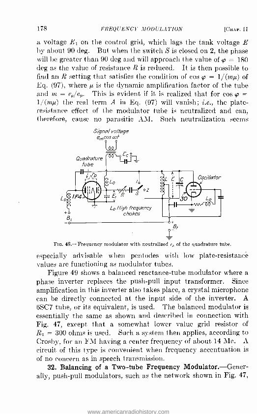
178 FREQUENCY MODULATION [CHAP. II
a voltage E1 on the control grid, which lags the tank voltage E by about 90 deg. But when the switch S is closed on 2, the phase will be greater than 90 deg and will approach the value of cp = 180 deg as the value of resistance R is reduced. It is then possible to find an R setting that satisfies the condition of cos cp. = 1/(m) of Eq. (97), where ,u is the dynamic amplification factor of the tube and m = ea /ep. This is evident if it is realized that for cos cp = 1 ï (mµ) the real term A in Eq. (97) will vanish; i.e., the plate - resistance effect of the modulator tube is neutralized and can, therefore, cause no parasitic AM. Such neutralization seems
Signal voltage em cos Wt
Quadrature tube
jrp óLo
Lo High frequency chokes
lo
o
+n,
FIG. 48.- Frequency modulator with neutralized r1, of the quadrature tube.
especially advisable when pentodes with low plate -resistance values are functioning as modulator tubes.
Figure 49 shows a balanced reactance -tube modulator where a phase inverter replaces the push -pull input transformer. Since amplification in this inverter also takes place, a crystal microphone can be directly connected at the input side of the inverter. A 6SC7 tube, or its equivalent, is used. The balanced modulator is
essentially the same as shown and described in connection with Fig. 47, except that a somewhat lower value grid resistor of
R2 = 300 ohms is used. Such a system then applies, according to Crosby, for an FM having a center frequency of about 14 Mc. A
circuit of this type is convenient when frequency accentuation is of no concern as in speech transmission.
32. Balancing of a Two -tube Frequency Modulator.-Gener- ally, push -pull modulators, such as the network shown in Fig. 47,
www.americanradiohistory.com

SEC. 32] AUXILIARY APPARATUS
T
II
O ó O --NA/-)- L,) t
179
www.americanradiohistory.com

180 FREQUENCY MODULATION CHAP. II
have, the advantage of giving twice the frequency swing and also the advantage that any voltage fluctuations occurring in the power -line supply voltage can be made ineffective as far as the stabilization of the center frequency and all the important side frequencies are concerned. This is accomplished by superimpos- ing on the push -pull modulator action a small and suitable push - push modulator action. Such a superimposed action can be made to offset any reaction between the oscillator frequency and the power -supply voltage. The superimposed push -push action is effected by a small off balance of the respective modulator sections.
To do this we first obtain modulator balance such as is required by the balancing condition given in Fig. 47. Since the Coe capaci- tance is small and rather indefinite, as far as the actual measure- ment is concerned, it seems best to use a value for the series resistor R1 large enough so that essentially only the resistor is responsible for the magnitude of the current flow I1 due to the tank voltage E. A value of R1 = 50,000 ohms will accomplish this. Using a 1,000 -ohm resistor from the control grid of the lower modulator tube to ground and a two -plate midget condenser of 0 -2 µµf in series with it provides a ready means for adjusting the balance. For no signal voltage e,,,, cos wt acting, the primary center frequency F should result. Suppose we want to use the balanced modulator in connection with a transmitter, where eight- fold frequency multiplication follows the primary FM and the assigned carrier frequency of the radiated wave is 44.5 Mc. We have, then, a primary center frequency F = 44.5/8 = 5.5625 Mc. The next step in the adjustment of the modulator is to vary the variable condenser C of the tank until no beat note is obtained against a standard frequency source which has an integral rela- tionship with respect to 5.5625 Mc. This is done with the midget condenser C2 at its mid- capacitance setting. If the supply voltage is varied, say over ± 10 per cent of its normal value of 115 volts, and a beat note is heard again, then a value of the C2 setting is found for which F remains essentially fixed. This adjustment may be called the unmodulated carrier- frequency stabilization toward line -voltage fluctuations. To meet also the actual FM condition, we have to apply FM for maximum permissible frequency devia- tions and repeat the procedure by beating against the carrier.
A maximum voltage em in em cos wt is impressed on the balanced modulator of Fig. 47, such that em corresponds to a maximum
www.americanradiohistory.com

SEC. 32] A UXI LIA RY APPARATUS 181
frequency swing of ± 75 kc in the radiated wave. This leads to ß values, even for the maximum audio frequency fa,ax = 15 kc, as large as ß = 7yí5 = 5, and eight significant side currents on each side of the carrier frequency appear. This can be seen from Table III on page 33. This table also shows that the amplitude of the carrier frequency is only 17.7 per cent of the unmodulated carrier Im; some of the side currents have much larger amplitudes. It seems, therefore, more convenient to work with a reduced carrier frequency, such as the primary center frequency of 5.5625 Mc in this particular example. There is then a corresponding maximum permissible frequency excursion of only 758 = 9.375 kc. For the highest signal frequency fn,ax = 15 kc, there is a ß value of only 9.375/15 = 0.623 radian. According to Table III, essentially only two additional side currents on each side of the center fre- quency then exist. According to Table I on page 20, we now have a center- frequency amplitude of essentially 90 per cent of the unmodulated carrier level. It is, therefore, much easier to make the center -frequency check directly on the primary FM current modulated to the largest permissible frequency swing. It is to be understood that any resetting of the small condenser C2
requires also a slight readjustment of the tank setting of C.
If it is of concern only to balance the modulator of Fig. 47, irrespective of any frequency drifts due to line -voltage drifts of the supply voltage, it is only necessary to tune in with an FM receiver on the radiated wave to be tested with respect to modulator balance. We have then two possible procedures. One is to operate the transmitter with the modulator in the normal condition, i.e., with the normal connection in push -pull. When the C2 setting is varied for an em amplitude corresponding to the highest permissible frequency deviation in the radiated wave, then the greatest FM, i.e., the loudest reception, will be noticed in the receiver for correct balance. But as far as the sensation in the human ear is concerned, it is quite difficult to distinguish between loud and somewhat louder sounds. This is especially true when a certain pronounced loudness exists. The second procedure avoids this difficulty since for it the respec- tive modulator grids are connected together; i.e., they act in parallel. This yields a push -push modulation for which the injected i, variation due to the upper modulator tube tends to cancel the effect of the simultaneous injected i variation due to the
www.americanradiohistory.com

182 FREQUENCY MODULATION [CHAP. II
lower modulator tube. Hence, when this modulator connection is used during the modulator adjustment, the setting of the C2
condenser is varied until minimum sound is noticed in the FM receiver. Theoretically, no FM should exist. Thereafter, during normal operation the modulator is connected with the control grids as indicated in Fig. 47.
33. Phase Modulators.' Generally, it may be said that in FM we have higher plate efficiencies in the respective power stages than for AM systems, on account of the feature of constant carrier level In,. This is, of course, also true for PM systems. The modulation apparatus required in PM systems is simpler than that used in AM systems. It is also possible to produce PM at low - power levels since amplitude linearity in the power stages is of no concern for phase variations. Even though the main purpose of this treatise is to describe systems for FM, it must be recalled that, in indirect FM, phase modulation is instrumental in bringing about all the features of direct FM. Such features exist as far as the final stages in the transmitter are concerned as well as in the entire FM receiver.
With respect to the description given in connection with Fig. 3, we understand that PM can be accomplished with a network such as is shown in Fig. 50. In Fig. 50a, two equal tubes are connected in parallel, as far as their plate outputs are concerned, with respect to the common external plate load, which is a CL tank tuned with respect to the carrier frequency F. It will be noted that the modulating or signal voltage em, cos wt drives the two tubes in algebraic push -pull. As far as the respective control grids are concerned, the tubes are driven in geometric push -push with respect to the voltage Em sin Sgt of carrier frequency F. By algebraic push -pull is meant the customary push -pull input voltage where at any instant equal but opposite voltages act on the respective grids. Owing to the C1R1 network across the carrier - frequency source as well as across the respective control grids,
1 ARMSTRONG, E. H., A Method of Reducing Disturbances in Radio Signaling by a System of Frequency Modulation, Proc. IRE, 24, 689, 1936. LAUTENSCHLAGER,
F., Phase Modulated Oscillators, EN7', 11, 357, 1934. CROSBY, M. G., Communica- tion by Phase Modulation, Proc. IRE, 27, 126, 1939 (this paper gives about the best account on useful devices in PM). Yocum, C. H., Frequency Modulation, Part II, Communications, 19, p. 14, December, 1939, (this article describes also the R. E. Shelby phase modulator). SABAROFF, S., New System of Frequency Modulation, Communi- cations, 21, p 8, September, 1941.
www.americanradiohistory.com

SEC. 33] AUXILIARY APPARATUS 183
the control grid-to-cathode path of one tube is exposed to an applied voltage á 1, which is a sine function of carrier frequency. The control grid -to- cathode path of the other tube is exposed to a voltage g2, which is a cosine function of the carrier frequency. Therefore, the respective tubes are driven in quadrature push -push. On account of the chosen reactance value of condenser C1 at the carrier frequency F, there are at any instant quadrature voltages of equal values acting on respective control grids.
PM- Curren!
C
Tube2
Co
A2=Ern COS Al' --Y
' 628 FC,
á- Emsinllt >O Source of carrier
frequency F
.Q99bQ90,
em coscvt (v
I IG. 50.- Production of phase -modulated currents.
As far as the input is concerned, we have the vector Oa for zero modulation voltage in Fig. 50b for the voltage Em sin Ot
of the carrier -frequency source. The applied control voltage (Em sin S2t) /-V2 on tube 1 must be in phase with vector g and is indicated by vector 0a1; the equal quadrature voltage applied to the other tube is the vector 0a2. The resultant of vectors ái and á2 is the vector OP. This vector must have the same scalar value as vector Oa. The 45 -deg time delay of OP with respect to the voltage Oa of the supply is not directly active at the input side, but for a unity grid -into -plate branch action, on account of the parallel connection, would represent the resultant tank voltage E.
(b )
www.americanradiohistory.com

184 FREQUENCY MODULATION [CHAI'. II
Voltage E would generally be proportional to voltage OP. There- fore, we may take the vector OP as the measure for E with respect to size as well as with respect to relative position when no modula- tion is taking place.
Now suppose that the signal -voltage e, cos cot is acting at an instant when wt = O. This is the instant of time indicated by the cosine trace in Fig. 50a. Then em will add algebraically to al in tube 1 and em will subtract algebraically from amplitude a2 in tube 2. Then we have in Fig. 50b the respective instantaneous carrier voltages OP1 for tube 1 and OP2 for tube 2. The resultant voltage, as far as the output network is concerned, is OP1. After 1/2f sec, -e, is superimposed on the control voltage of tube 1 and +en adds on the control grid of tube 2. This causes the instantaneous voltages OP; on tube 1 and OP2 on the control grid of tube 2, with the resultant vector OP which causes the value of the tank voltage E. Hence, the effect in the output branch of the modu- lator tubes is a phase fluctuation ±M and the peak -to -peak phase swing equal to the time delay of OP with respect to the supply voltage E, sin Sgt.
It will be noted that for such large M swings as are shown in Fig. 50b, a certain amount of harmonic distortion must be expected. Simultaneous AM occurs because the extreme vectors OP, and OP are somewhat longer than the correct vector size given by the radius of the circle. To remove the superimposed AM at the output side of the phase modulator by means of an amplitude limiter would also remove some of the useful modulation energy as is explained on page 59. It is, therefore, better engineering practice not to work with the equal amplitudes a1 and a2 at the input side, but with amplitudes that cause an angle a0P of not more than about 23 deg. Then M < 11.5 deg or about <_ 0.2 radian for which values the extremities of vectors P, and P will remain on the circle of radius a.
Figure 51 shows a block diagram of a phase modulator where the modulation product k1(KI , cos wt) sin Sgt is produced by a balanced amplitude modulator (page 187). The sinusoidal output current of a fixed carrier frequency F divides itself between a buffer amplifier and a balanced amplitude modulator which is also affected by a signal current i, cos wt. The constant kl takes care of the modulator efficiency and K is the degree of amplitude modulation obtained. A 90 -deg phase shifter causes a modulator
www.americanradiohistory.com

SEC. 33} AUXILIARY APPARATUS 185
output current of ki(KIm,, cos wt) cos Sgt. The output of the buffer amplifier delivers a current a = Um sin Sgt, where k stands for the gain of this amplifier. Since the two instantaneous
Fixed F- source
rm K= jm
k, modulator efficiency
k buffer amplifier efficiency
Im sinl2t
Imsinllt
Buffer I klmsrhl2t =á
amplifier dx'
b =k,Klm (cosu,f)(Cosllf)
Balanced amplitude
90- degree I
I
modulator k , KI m (aswt)(sinl2f) -b phase shifter
Tim cos cot
If- source)
i
wt= 90 °
(a)
fseconds
wt°lBO° col -270°
+d671 I-*-I dB
wt=360°
fdB
.;Imsin[628F7`4dBsin cot]
a b, b2
tdB
(b)
a = klm of frequency F; b, portion of b of frequency Ftf; b2 portion of b of frequency F -f; b,=05 k, 1?7 =b2
FIG. 51. -True phase modulation with maximum deviations ± O and modulation index ß = AB radians.
currents are in time quadrature at any moment, they must be
added vectorially at the mixer of the input of the last amplifier.
Hence, the current a + jb = V a2 + b2 flows into the mixer with an instantaneous relative phase tan-' (h /a). Since cos Sgt cos wt
www.americanradiohistory.com

186 FREQUENCY MODULATION [CHAP. II
= 0.5[cos (S2 + co)t + cos (0 - co)t], we have for k1K = k2 the instantaneous mixer current
It = kIm sin SZt + 0.5k2Im cos (SZ + co)t + 0.5k2Im cos (S2 - co)t _ + b1 + 1)2 (124)
As far as the modulation is concerned, we are interested only in the cycle of the modulation frequency f, and not in the cycle of the instantaneous carrier frequency Ft, which for amplitude modula- tion happens to be equal to the center frequency F. We have, therefore, the expressions
b1 = 0.5k2I m cos (Qt + wt)
1 b2 = 0.5k2Im cos (Qt - wt) (125)
which at the instant t = 0, for the signal frequency f, yield b1 = 0.5k2Im cos Sgt = b2. But k2 = k1K = kiim /Im; hence b1 = b2 = 0.5kiim cos SU and
It = Io = AI, sin Sgt + 0.5kiim cos Sgt + 0.5klim cos Sgt
= a + j(b1 + b2) (126)
where b1 = b2 = 0.5k1im. Equation (126) also shows that there is a phase deviation AO = tari 1 [(b1 + b2) /a] = tan-' (kiim /kIm) = tan-1 (k1K /k). Therefore, if the modulator efficiency were 100 per cent and no buffer amplifier were used, we would have M = tan-1 K, where the argument K is the degree of AM in the balanced modulator. For 20 per cent AM we would have LB = tan-' 0.2 = 0.2 radian, or about 11.5 deg. The corresponding vector addition is shown in Fig. 51b at the instant when cot = 0.
For wt = 90 deg we have, then,
I t = I oo = kIm sin Qt + 0.5klim cos (Qt + 90) + 0.5kiim cos (SZt - 90) = kIm sin Sgt - 0.5kiim sin Sgt + 0.5klim sin Qt = a - b1 + b2 = a (127)
since b1 = b2 = 0.5klim. We have, therefore, no phase swing at this instant of time as can also be seen in Fig. 51b. The effects of the upper and lower side currents of respective frequencies F ± f cancel because they are in antiphase and in phase with the carrier - frequency amplitude a = kIm. At the moment for which cot = 180 deg, we find
It = Iiso = kIm sin Sgt - 0.5k1Im cos Qt - 0.5k 1/,,, cos Ot = a - j(b1 + b2) (128)
www.americanradiohistory.com

SEc. 33] AUXILIARY APPARATUS 187
and we have a negative phase swing in Fig. 51b. We have for this swing M = tan' [- (bi + b2) /a]. For wt = 270 deg, we find
I27o= a +b1 -b2 =a (129)
which means that again this is an instant of time on the signal - frequency cycle for which no modulation can occur. I360 is
naturally the same case as Io. We note, therefore, that linear PM occurs, since the instan-
taneous phase swings during the modulation cycle are directly
Unmodu/ated carrier current
Buffer amplifier..
T ';I 4(1
+Ec Piézo oscillator of fixed primary fmsmlltl frequency F
alc) J
Balanced amp/dude modulator
Combines carrier with I phase-shifted
modulation product - - - - - --i
I
Ts I
I > V
I PM- Current
- 14+ -82+_i YI
-Phase- shifted modulation product
Ì _T '
L :II I
I IL, L: II
1 EBO- I
t c LI -z c - -
J 90- degree phase shifter
6.28F= (CLI- "z
J
Illo olY em cos cut Signa/or
modulation voltage
Amplifier of modulation
product
FIG. 52.- Generator for a true PM current with a modulation index ß = O8.
proportional to the instantaneous value i, cos wt of the signal current which causes the modulation. Also here the limitation applies that, for distortion -free PM, the maximum ±M swings, occurring when the maximum values i, of im cos wt act, should not exceed 0.2 radian.
Figure 52 shows an actual network based on the block diagram of Fig. 51 where, in addition, an amplifier for the modulation product is used, which also acts as a buffer stage. We note that a
piezo oscillator of stabilized primary or master frequency F feeds into the buffer tube T3, as well as in push -push to the control grids
www.americanradiohistory.com

188 FREQUENCY JIODULATION [CHAP. II
of like modulator tubes T1 and T2 while the output plates of these tubes are connected in push -pull. Hence, no carrier current can flow in the output coil L1 in absence of a signal voltage em, cos wt. The signal voltage affects the second set of modulator grids in push -pull, and must, therefore, produce the modulation product. The inductive reactances of the primary output coils L in the respective modulator plate branches are neutralized by means of the capacitive reactances of the condensers C, with respect to the carrier frequency F. Hence, the plate variations due to the carrier -frequency source must be in phase with the driving carrier- frequency voltages acting on the respective grids of the modulator tubes T1 and T2. The natural period of the secondary L1, which applies its voltage to the control grid of tube T4, is very short compared with the period of 1/F sec of the carrier current. Hence, voltages induced in. L1 must be either 90 deg ahead or lagging, and the modulation product coming from the two L coils is shifted 90 deg in phase as far as the input and output actions of the amplifier with tube T4 are concerned. Hence, at the input side of the mixer amplifier we combine again a ± jb and cause PM as explained in connection with Fig. 51.
The network of Fig. 52 is the network used by Armstrong, except that a voltage which is proportional to (em, cos wt) f is applied at terminals III and IV. Therefore, the current emerging from terminals V and VI is not a true PM current at all, but is in effect an FM current since it has a maximum phase shift that is proportional to AO f. This has exactly the form of OF /f. When M in radians is numerically equal to OF, we shall have the same number of side currents in either case and for any signal frequency f the identity M f = SF /f holds.
In the commercial Armstrong transmitter not only does a correcting network for the 1/f effect precede the input terminals III and IV, but also a correcting network for a -f preaccentuation having a time constant of about 100 µ sec. This latter correcting network should follow directly the microphone since its purpose is to offset any of the undesired noises in the upper a -f range of frequencies.
We note, therefore, that in the Armstrong system there is primarily balanced AM. In virtue of the 90 -deg phase shifter in the output branch of the balanced modulator, the modulation product adds itself, at any instant, in quadrature with an unmodu-
www.americanradiohistory.com

SEC. 33] AUXILIARY APPARATUS 189
lated current of carrier frequency F. The effect is that PM is produced. But, owing to the amplitude em /f of the signal current, the PM experienced has all the features of direct FM. This means that the same energy distributions exist in the frequency spectrum for the entire a -f range as though FM were operative. We obtain, therefore, indirect FM. The primary indirect FM is, however, very small' since the corresponding extreme phase swings for allowable values of distortion should never exceed values of about 0.2 radian. Allowing only a small amount of harmonic distortion in indirect FM, phase swings larger than about ± 30 deg should be avoided.
At this point it should be understood that, when PM is caused by the addition of two out -of- please currents, such a limitation of maximum phase swings also must be met, if distortion is to be kept low. But if the relative phase O of the unmodulated current In,, sin (Qt + B) can be changed directly, and not by geometric addition, then large phase swings can cause PM without harmonic distortion since simultaneous AM is avoided. It does not seem helpful, therefore, to consider schemes where large phase swings result and geometrical addition is instrumental in bringing about wide -phase swing modulation. It is, however, true that we can cause wide -phase swing modulation, even in the Armstrong system, as long as we keep together, in the transmitter as well as at the reception end, the AM and the PM or the FM, whatever may be the combination. The only drawback in such a doubly modu- lated system would be that, at first, in the power amplifier stages there would not be such high plate efficiencies as with pure FM
1 There seems to be much confusion in current literature about the concept of PM in the Armstrong system. Some writers give the impression that we deal at first with PM because the FM is so small that we actually have only small phase liberations. It should, therefore, be clearly understood that the order of magnitude does not and cannot make of an FM effect a PM effect. If it is an FM effect for wide -band FM, i.e., after frequency multiplication, then it is also an FM effect for a very narrow hand FM. It has been brought out in Chap. I over and over again that there is a great difference between PM and FM. For PM the number of significant side currents is, for a fixed maximum phase swing, independent of the order of the signal frequency f. This is not true for FM since for a fixed maximum frequency swing the number of significant side currents decreases as the signal frequency f increases. In other words the dis- tribution of the modulation energy for FM is generally different from the energy distribution for PM. It is the energy distribution of the modulation energy that counts. Since in the Armstrong system, after combination of the carrier current with the phase -shifted modulation product, the inverse ] f effect also exists, we have throughout an FM effect, no matter how small it is to begin with.
www.americanradiohistory.com

190 FREQUENCY MODULATION [CHAP. II
or with pure PM systems. Secondly, the very feature of high signal -to -noise ratio characteristic of FM would be defeated, since amplitude limiters could not be used.
When the output of an oscillator, whose frequency F is " stiff," is affected, for instance, by a reactance tube, the result will be a PM with quite large phase swings instead of direct FM. The reason for this is that a stabilized frequency F, as in a piezo source, will not allow phase balance and the resultant oscillator current will so to speak "give way" and will yield to periodic phase shifts. What will occur then is an oscillator current which "as a whole" shifts forward and "as a whole" shifts backward without changing the number of cycles within the current wave, which is shifted "as a whole." In other words the entire current wave shifts to and fro along the time axis and, as such, is kinetic with modulation energy that can be separated by phase demodulation. It is true that we have equivalent frequency variations, but we should not confuse equivalent frequency modulation with real changes in the carrier frequency where the time intervals between successive current maxima are not equal as in PM.
Hence, one way of causing PM would be to apply a voltage of a stabilized frequency F to the grid of a pentode tube and to tune the plate output tank circuit to the carrier frequency F with a quadrature tube network in parallel with the plate tank circuit. This assumes that the modulation voltage is not acting. But when the signal voltage en,, cos wt is also present, the plate tank current will be modulated in phase since the frequency F is "stiff." A coupled circuit feeding into a load experiences, therefore, a PM current.
It was shown' how a cathode -ray tube acted upon by two high - frequency voltages, which are in space quadrature as well as in time quadrature and affecting a cathode ray, can be made to show a spiral fluorescent pattern if the two voltages are modulated in amplitude. Using such an arrangement, we have the illustration of Fig. 53a where a piezo generator of stabilized carrier frequency F feeds into a modulator which, on account of the signal voltage em, cos wt, causes AM. The output of the modulator feeds into a 90 -deg phase shifter and then affects the respective deflection plates P,P2 and P3P4 of a cathode -ray tube. Figure 53b shows
I "Phenomena in High- frequency Systems," pp. 146, 157; "High- frequency Meas- urements," pp. 373 -374.
www.americanradiohistory.com

SEC. 331 AUXILIARY APPARATUS 191
that a circular fluorescent cathode -ray trace is obtained when no modulation voltage em cos wt is present. For a certain degree K of amplitude modulation, a concentric fluorescent ring of width W appears on the screen of the cathode -ray tube. In reality the fluorescent ring is a spiral trace which shrinks and grows according
r IPiezo oscillatori I of primary
frequency F L ° °
r- I,,,sinllt
Amplitude modulator
L_p _q J Signal emcosWt
5
P3I
Spiral fluorescent cathode spot trace
For pure AM, spot P traces shrinking and growing spirals within width Wand //near arrangement of points I- 2- 3-4- 5 -6 -5 -4 etc If PM exists simultaneously curved recurrences l-2=3'-4= 5 -f6eíc. and de maximum phase deviation
FIG. 53.- Determination of superimposed phase swing AO in an amplitude- modulated cur- rent with parasitic PM.
kEmsinllt -kem sin rat
kE,,, ' b1ÌÌ.
I
I
l' No modulation (cathode spot P amplitude mplitud> traces circular módulatiai modulation trace)
(b)
(q)
ErEZ =W
E,-EZ
_ um
I,,,
to the signal- frequency modulation. At any instant the vector of the trace, which rotates with the angular velocity 6.28F, has a length that is proportional to Em(1 -}- K cos wt), the constant of proportionality being k. Since, for pure AM the extremities 1, 2, 3, 4, etc., of the rotating vectors, which occur 1/F sec apart, must lie on a radius as OP, we have a means for finding out experi- mentally when PM also exists in addition to AM. If PM exists
www.americanradiohistory.com
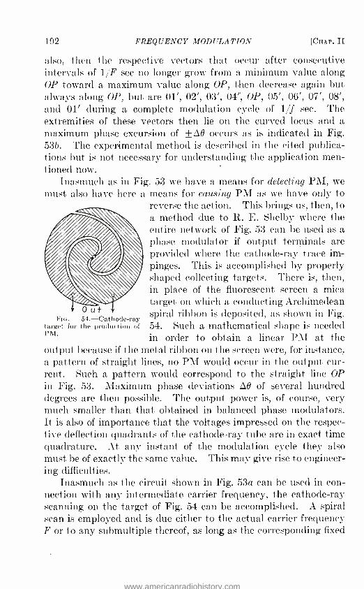
192 FREQUENCY MODULATION [CHAP. II
also, then the respective vectors that occur after consecutive intervals of 1/F sec no longer grow from a minimum value along OP toward a maximum value along OP, then decrease again but always along OP, but are 01', 02', 03', 04', OP, 05', 06', 07', 08', and 01' during a complete modulation cycle of 1/f sec. The extremities of these vectors then lie on the curved locus and a maximum phase excursion of ±M occurs as is indicated in Fig. 53b. The experimental method is described in the cited publica- tions but is not necessary for understanding the application men- tioned now.
Inasmuch as in Fig. 53 we have a means for detecting PM, we must also have here a means for causing PM as we have only to
reverse the action. This brings us, then, to a method due to R. E. Shelby where the entire network of Fig. 53 can be used as a phase modulator if output terminals are provided where the cathode -ray trace im- pinges. This is accomplished by properly shaped collecting targets. There is, then, in place of the fluorescent screen a mica target on which a conducting Archimedean
O u t spiral ribbon is deposited, as shown in Fig. FIG. 54.- Cathode -ray
target for the production of 54. Such a mathematical shape is needed PM. in order to obtain a linear PM at the output because if the metal ribbon on the screen were, for instance, a pattern of straight lines, no PM would occur in the output cur- rent. Such a pattern would correspond to the straight line OP in Fig. 53. Maximum phase deviations M of several hundred degrees are then possible. The output power is, of course, very much smaller than that obtained in balanced phase modulators. It is also of importance that the voltages impressed on the respec- tive deflection quadrants of the cathode -ray tube are in exact time quadrature. At any instant of the modulation cycle they also must be of exactly the same value. This may give rise to engineer- ing difficulties.
Inasmuch as the circuit shown in Fig. 53a can be used in con- nection with any intermediate carrier frequency, the cathode -ray scanning on the target of Fig. 54 can be accomplished. A spiral scan is employed and is due either to the actual carrier frequency F or to any submultiple thereof, as long as the corresponding fixed
www.americanradiohistory.com

SE( '. 34J A('X ILI :II/Y Al'l'ARAT('.S 193
angular velocity G.28F can accommodate the signal modulation speed of 6.28f. It is this speed that causes the circular cathode - ray trace periodically to increase or decrease in diameter as the vector, due to the carrier angular velocity 6.28F, spins around. Even though such a system may give rise to practical difficulties as far as the balancing of the deflection voltages is concerned, it may he said that a more true PM can be produced when such difficulties are overcome. The reason for this is that the cathode - ray tube gives a very good buffer action toward the source that excites it.
We have to realize that we are interested in pure PM and not in PM with partial superimposed FM. Now, the producing of a modulation along the time axis of a current wave can do both: it can change the carrier frequency directly or only the phase. It can also affect both types of time axis modulations. Pure PM without direct. FJI effects is possible only when the sinusoidal wave train is moved to and fro about its fixed relative phase position without, so to speak, "squeezing" or "stretching" the con- secutive current waves together or apart during to -and -fro oscilla- tions of the entire wave train. In this system we have to begin with a "stiff" frequency F, since it is due to a piezo source, and we can hardly imagine any back action on the magnitude of F from the collector electrodes on the mica screen. Hence, we may assume that no superimposed FM can exist.
At this point it 5110111(1 be realized that even though any frequency demodulator can be readily converted into a correct phase demodulator, and vice versa, by adding a simple correcting network (described in Sec. 34), this remedy cannot be used when both types, i.e., FM and PM, act simultaneously.
34. Commercial Demodulators. -In Sec. 15 dealing with the translation of FM into A?I, the fact was discussed that a frequency discriminator will translate FM variations as well as PM variations into corresponding AM variations. These amplitude variations will, in turn, give also an inherent a -f output, owing to the ampli- tude demodulator action of the rectifiers used in the discriminator.
The fact that a discriminator can translate either FM or PiI into a -f variations does not mean at all that the audio output is correct as far as the relative amplitudes of the various audio frequencies f at the transmitter end are concerned. The separa- tion of the various audio components in a frequency discriminator
www.americanradiohistory.com

194 FREQUENCY MODULATION [CHAP. II
is correct for impressed FM voltages, since the discriminator is designed for reversing the action of the FM caused in the transmit- ter. It is not correct, however, when PM voltages are impressed on a frequency demodulator since the translation is not due to phase discrimination but to equivalent frequency discrimination. From Eq. (6) we learned that the equivalent frequency deviation about the true and fixed carrier frequency F is f AO cos wt. Hence, it increases with the pitch of the sound heard or causes a -f accen- tuation toward the higher audio frequencies.
This can be readily remedied by connecting, between the audio output of a frequency discriminator and the a -f amplifier of an FM receiver, a correcting network which compensates for the f effect by means of a 1/f effect. All that is necessary is to connect a series combination of a resistance and a condenser across the output of the discriminator and to apply the condenser voltage to the a-f amplifier. That a 1/f effect is produced thereby is seen from the fact that the uncompensated fin?, cos wt current is propor- tional to the amplitude Jim instead of only to im and flows through both the resistance R and the condenser C. It causes a voltage across the terminals of the condenser which is proportional to im f cos wt dt, the constant of proportionality being 1 /C. The integration gives a value that is inversely proportional to the signal frequency f and cancels the f effect in fine. A voltage that is proportional only to im is, therefore, applied to the a -f amplifier.
A direct phase -to- amplitude translation can be obtained by reversing the action illustrated in Fig. 3. In connection with this figure, we learned that PM can be caused by adding in quadrature to the unmodulated vector a the modulation product b obtained in AM. The product b of Eq. (2) can, according to Eq. (3), be split up into the upper and lower side currents of respective frequencies F ± f if the maximum phase deviation is not much more than about 11.5 deg. Otherwise, an AM effect due to the other side currents given in Eq. (3) would also exist. Since phase demodula- tion is the opposite action to that shown in Fig. 3, it is only neces- sary that the PM demodulator shift the phase of the carrier with respect to the side currents by 90 deg, or vice versa, in order to obtain AM. Customary amplitude demodulation then follows in order the extract the a -f currents. When, for instance, a crystal filter is used without completely neutralizing the crystal- holder capacitance, then PM into AM translation takes place.
www.americanradiohistory.com

Si.c. 35] AUXILIARY APPARATUS 195
35. Actions in Frequency Discriminators. -Since frequency dis- criminators are used not only as FM -AM converters, hut also for center -frequency stabilization in FM transmitters, a brief descrip- tion of the actions in such apparatus is given here.' Frequency discriminators are more or less adaptations of the well -known Seeley type of a -f -c discriminator. They are, therefore, basically a primary branch, which is tuned to the center frequency F, and a secondary system, which gives no unidirectional output voltage if the desired center frequency F prevails. It gives, how-
Input
Amp/dude
tE,when L, and L2are indirect series
4F- F
AAmplitude
when L, and L2 are indirect series
C,L, =C2L2 and tuned to -dF F - +dF center frequency F
Flo. 55. -- Actions in doubly tuned circuits.
ever, either positive or negative output voltages for all instan- taneous carrier frequencies Ft that are close to F and within the peak -to -peak frequency swing for which the discriminator is designed. For frequency demodulation the design has to be for a width of at least 150 kc. There are also other types of FM to AM converters but they are not in common use.
Generally, when an emf is induced in a loosely coupled tuned secondary circuit, owing to a resonance current flowing in a tuned primary circuit, the voltages across the respective primary and secondary coils are 90 deg out of phase. When such circuits are connected in the output branch of a vacuum tube, as in Fig. 55, LI is the primary coil and L2 is the secondary coil. Since E, is
' TRAVIS, C., Automatic Frequency Control, Proc. IRE, 23, 1125, 1935. FosTER, I). E., and S. W. SEELEY, Automatic Tuning, Simplified Circuits, And Design Prac- tice, Proc. IRE, 25, 289, 1937. GRAMMER, G., and B. GOODMAN, Wide Band Fre- quency Modulation in Amateur Communication, QST, January, 1940. CROSBY, M. G., Reactance Tuhe Frequency Modulators, RCA Rev., 5, 89, 1940. WElss, W., Detection in FM Receivers, Communications, 21, p. 16, March, 1941. LEVY, M. L., Frequency Modulation Receivers, Comnnunicalions. 21, p. 5, March, 1941.
www.americanradiohistory.com

196 FREQUENCY MODULATION [CHAP. II
the driving voltage that causes the resonance current flow I, of frequency F, a voltage E2 which is 90 deg out of phase is pro- duced in the loosely coupled secondary coil L2. The absolute magnitude of the resultant total voltage E in the neighborhood of the resonance frequency F is then as indicated by the E curve. We have to distinguish between two relative coil connections. In one connection, the double -pole double -throw switch 1 -2 is on 3 -4 and the fields of coils L1 and L2 are additive; for the other con- nection, 1 -2 is on 5 -6 and the inductances act in indirect series. The fields are, therefore, subtractive. For this reason, the respective E curves are in a mirror symmetry with respect to the amplitude reference axis.
11= 6.28F =i FIG. 56. -How a frequency- discriminator characteristic can be obtained.
Hence, if we desire a system that reacts only when frequency deviations .F' occur about the center frequency F but does not respond at its output when a center- frequency voltage is applied, we have only to use a differential action in a network that is driven by the voltages E1 and E2. This is indicated in connection with the network of Fig. 56, where we likewise obtain symmetrical output voltages E, and I''', and the difference voltage E1 -E11 gives the desired characteristics. Since in Fig. 55, for one switch connection, we have a positive coupling and, for the other switch connection, a negative coupling between primary and secondary tuned circuits, the potential at either end of the secondary winding with respect to the center tap of this winding must be 180 deg out of phase. For this reason the center tap, instead of one end of the secondary, is connected to the primary in Fig. 56. With such a
direct connection from primary to secondary, the respective output voltages E1 and E,, give likewise maximum values on each side of the "mirror or amplitude axis." We note, therefore, that for the center frequency F, the voltages E, and Ell have equal ampli-
Ez -Ea
www.americanradiohistory.com

SEC. 35] AUXILIARY APPARATUS 197
tude values. Also for frequencies that are deviated by the same amount +ZIF above the center frequency F and below it, we have equal E, and E values. Even though the difference effect E1 -E1, could be obtained directly in a network properly connected to terminals a, b, and c of Fig. 56, a preferred form is to apply the respective voltages E, and E,, to two like and separate rectifiers and then to add the resultant direct voltages at the output side in opposition. In this way there can be no direct output voltage at the center frequency F, while at frequencies F ± OF, equal direct voltages of opposite polarity occur at the output side of the
=C2L2
Center frequency f= 1nC,C,
1
d E,,,sin(22rtdt modulated input F instantaneous intermediate
carrier frequency
Small reactance tbfj
LL2
L,
C4 is a small reactance 6116 atlowes/signa/ 2 frequency f
a d
M -Ea
¡El Ló -
Direct 9p voltage
b o Audio Cs 1 h voltage If
R, and R2 are essentially equal and from 0.5 to lx/06ohms
Lo High Diréc/ frequency current
choke 1=11412 FIG. 57.-Frequency discriminator for obtaining direct output voltage r..> well as audio -
frequency recovery.
discriminator. The polarity for the resultant output voltage for a frequency F OF is then in opposition to the polarity of voltage for frequency F - LOF since we are dealing now with a balanced frequency discriminator. It can be shown that in tuned coupled circuits such as are used here having the same Q value in the primary as in the secondary, when coupled critically together, the best discriminator condition obtains if the secondary induct- ance is twice the value of the primary inductance. For such a condition the greatest rate of change occurs in the absolute magnitude of the resultant of two voltage components, which are 90 deg out of phase, when small changes in the angle between the components occur. Hence, the largest possible difference voltage will be obtained at the output.
Figure 57 shows how the difference effect is obtained. Tube T1 serves the purpose of producing a driving voltage E1 across primary inductance L1 of the double -tuned transformer L,, L2. This voltage is then affected when the instantaneous carrier frequency Fr changes. The coupling condenser C3 is the direct
www.americanradiohistory.com

198 FREQUENCY MODULATION [('nAe. H
connection to the center tap of the secondary; hence, it must be dynamically a short circuit to currents of frequencies Fr. Since the center tap of L2 connects to the mid -point of the respective external rectifier resistors R, and R2, a rectified current must flow from b toward the center tap of L2. The resistances R1 and R2 have large values and are usually equal to about 0.1 to 1 megohm for essentially equal tube halves of a 6H6 twin rectifier. Hence, the rectified current must divide itself equally, flowing through the linearity resistance R1 from the cathode of the upper tube half and through the linearity resistance R2 from the cathode of the lower tube half. Since the purpose of the condenser C4
is to connect the respective cathodes dynamically together with respect to F, frequencies, we note that the h -f voltages E, and Ell have such effects on the direct potential at point a with respect to ground that for the center frequency we have E1 = E11. Hence, this potential vanishes because the direct current flow through R1 and R2 is in opposition and causes equal and opposite direct voltages across terminals ab and bc.
But when the instantaneous carrier frequency has a value F, = F + OF', we note in Fig. 56 that E is larger than E, and we have the corresponding values e2 and el acting at the input side of the discriminator shown in Fig. 57. This means that the direct current flow I1 through R1 is now larger than the direct current flow I2 through resistor R2. Since the values of R1 and R2 are essentially equal, a certain positive potential results at terminal d with respect to ground. If the instantaneous frequency had had a value F, = F - OF ", we note from Fig. 56 that E = ez
would be smaller than E1 = e1'. Hence, in Fig. 57 the drop in R, would be smaller than the negative drop in R2, leaving a certain negative potential at terminal d with respect to ground. Hence, the output terminals d and g of the discriminator will give direct voltages with a polarity positive or negative, according to whether the instantaneous carrier frequency Fr is larger or smaller than the center frequency F. The terminals d and g are used when the discriminator is employed for stabilization of the center fre- quency F, since the output voltages can be made to change the fixed grid bias of a reactance tube. When the fixed bias of such a modulator tube is changed, the fixed reactance injection into an oscillator can be made to compensate the center-frequency drift of this oscillator.
www.americanradiohistory.com

SEC. 35] AUXILIARY APPARATUS 199
Inasmuch as in this network rectifiers are used, we have also inherent amplitude demodulation after FM -AM conversion has taken place. Since in Fig. 57 the condenser C4 has a reactance that is small, even for the lowest audio frequency of interest, both rectifier cathodes are essentially at ground potential as far as the useful a -f and h -f voltages are concerned. In this network the condenser C5 is needed only when a h -f choke is employed between the center tap of L2 and mid -point b. The use of such a C5 con-
Audio output
tH C4
C- Condensers have l low reactance to all F currents but high reactance tool/ audio currents ,,.
6116
2
Direct vo/is E
R=100k R=100k
8
6
4
a b C' 2
Last limiter tube of FM receiver
C3--
2 ó 0
C=Cu C=C1
I v EiÌ
_1 r' - f2 -E3
I
> 2
4
-6
8
P, IMMINIMINIIMUMoJ.7m IIIMIIIMIIINMP . ° MI MMIINIII 0. MINNIIII M (in 'has MIMI II MEMNON :45(Eleads E Z a: .IMMEIMMI EIMEIA I MIME... EIMENI M. MEMEIMMUME MgqI/BíziNMMIMMEI NIfMMIMMI
' 1ii -100 -50 0 +50 +100 kc
Frequency deviation 6F
Lead of E2 over Ei
Discriminator characíerisiic with respect to output direct voltage and phase between E2 and E, voltages
Fin. 58.- Discriminator connections as used in commercial apparatus.
e)
by45°l
6SJ7 or its equivalent
+B
denser and a h -f choke coil will decrease the effect of the resistors R1 and R2 on the Q value of the C1L1 branch. The magnitude of condenser C5 is so chosen that it has a high impedance even at the highest audio frequency of 15 kc, but a low impedance for any instantaneous carrier frequencies Ft. Hence, h is a potent a -f pole and terminals h and g will give directly an a -f output. The a -f output could also be taken off across terminals d and g if condenser C4 by- passes only h -f carrier currents and acts as a high reactance for the entire a -f range.
Figure 58 shows a symmetrical discriminator. Its actions are as shown in Fig. 59. In Fig. 58 the output of the two rectifier halves not only work into equal high resistances R but also use
www.americanradiohistory.com

200 FREQUENCY MODULATION [CHAP. II
equal condensers C which behave as low reactances at all carrier frequencies Ft but as high reactances at all audio frequencies. The a -f output is taken off through an isolation condenser C4
from the cathode that is dynamically high or potent with respect
(a)- Voltage E2 leads voltage E1 by 90 degrees, e = -e, positive (E1+E2) -caps cancel effects of negative (E,-1- E3) caps
tE2 Err E2
\. E3 £Z `
\ \
-e= EifE3
Condition for -e center frequency F
-E,4£2 'Charging condenser Cu of fig. 58
fE3
-- -T c -i----,.-. -e E2
Charges condenser C1 of fig. 58
(b)- Voltage E2 leads voltage E1 by 45 degrees, e' > -e ", positive (E, +E2) -caps larger than effect of negative(E, +E3) -caps, hence direct output voltage which is positive
FIG. 59.- Explanation of the cause of an output voltage.
to the other cathode, which is at ground potential. We have twofold power transfer from an i -f stage into the discriminator. One transfer is by means of the coupling condenser C3, which has a negligible reactance at all Ft frequencies. The other power trans- fer is by means of the mutual inductance of the discriminator
www.americanradiohistory.com
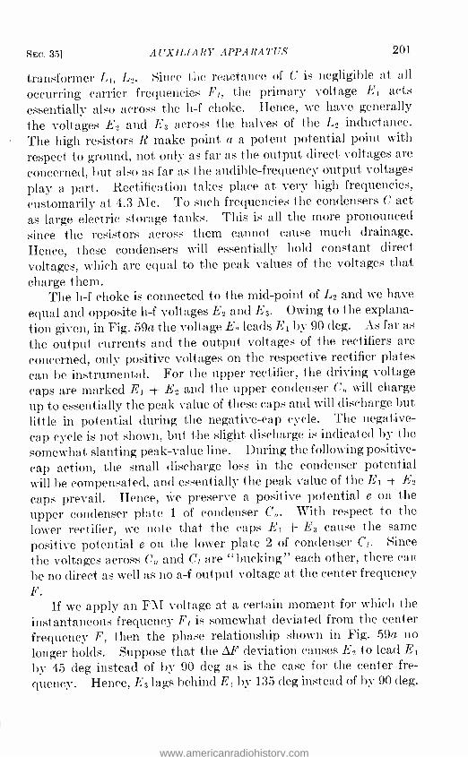
SEC. 35] AUXILIARY APPARATUS 201
transformer L1j L2. Since the reactance of C is negligible at all
occurring carrier frequencies Fr, the primary voltage E1 acts essentially also across the li -f choke. Hence, we have generally the voltages E2 and E3 across the halves of the L2 inductance. The high resistors R make point a a potent potential point with respect to ground, not only as far as the output direct voltages are
concerned, but also as far as the audible- frequency output voltages play a part. Rectification takes place at very high frequencies,
customarily at 4.3 Mc. To such frequencies the condensers C act as large electric storage tanks. This is all the more pronounced since the resistors across them cannot cause much drainage. Hence, these condensers will essentially hold constant direct voltages, which are equal to the peak values of the voltages that charge them.
The h -f choke is connected to the mid -point of L2 and we have equal and opposite h -f voltages E2 and E3. Owing to the explana- tion given, in Fig. 59a the voltage E2 leads E1 by 90 deg. As far as
the output currents and the output voltages of the rectifiers are
concerned, only positive voltages on the respective rectifier plates can be instrumental. For the upper rectifier, the driving voltage caps are marked E1 E2 and the upper condenser C will charge
up to essentially the peak value of these caps and will discharge but little in potential during the negative -cap cycle. The negative - cap cycle is not shown, but the slight discharge is indicated by the somewhat slanting peak -value line. During the following positive - cap action, the small discharge loss in the condenser potential will be compensated, and essentially the peak value of the E1 E2
caps prevail. Hence, we preserve a positive potential e on the upper condenser plate 1 of condenser Cu. With respect to the lower rectifier, we note that the caps E1 E3 cause the same
positive potential e on the lower plate 2 of condenser C1. Since
the voltages across Cu and Cr are "bucking" each other, there can
be no direct as well as no a -f output voltage at the center frequency F.
If we apply an FM voltage at a certain moment for which the instantaneous frequency Fr is somewhat deviated from the center frequency F, then the phase relationship shown in Fig. 59a no
longer holds. Suppose that the AF deviation causes E2 to lead E1
by 45 deg instead of by 90 deg as is the case for the center fre-
quency. Hence, E3 lags behind E1 by 135 deg instead of by 90 deg.
www.americanradiohistory.com
202 FREQUENCY MODULATION [CHAP. II
We have, then, the conditions depicted in Fig. 59b and note that the voltage caps E1 + E2 affecting the magnitude of the positive potential of the upper plate 1 of Cu give rise to a much larger e' value than the voltage caps E1 + E3 which cause the positive value e" on plate 2 of the lower condenser C1. The result is that point a is at a higher potential than ground, and a positive direct potential, as well as an audio signal, can be taken off at pole a with respect to ground.
In connection with this discussion it will be noted that the discriminator characteristic of Fig. 58 is limited, even though high linearity resistors R are being used in the respective load branches of the rectifiers. The limitation is due to the fact that at resonance, i.e., when both the primary and secondary circuits are tuned to the center frequency F, a 90 -deg phase shift occurs between the primary voltage E1 and E2 as well as E3. This is seen in Fig. 59a, where E2 leads E1 by 90 deg and E3 is 90 deg behind E1. But for any instantaneous carrier frequency such as Ft = F + SF', we still have antiphase relationship between E2 and E3, since the secondary coil L2 is center -tapped, but E2 leads E1 only by 45 deg. For a frequency deviation corresponding to the upper bend P1 of the discriminator characteristic, the voltages E2 and E1 are in phase and E3 and E1 are in antiphase, and vice versa, at the lower bend P2 of Fig. 58.
This can be realized from the fact that for all frequency values of Ft, the primary voltage E1 is, after all, responsible for any actions in the discriminator. The condenser C3 represents essentially zero reactance at all Ft values, and, therefore, E1 + E2 acts as the driving voltage on the upper rectifier. But at resonance frequency F, the secondary is tuned and must behave like a resistance load, which accounts for the quadrature addition E2 + jE1. If, therefore, the carrier frequency F is increased by an amount SF', the reactance of C2 decreases while the reactance of L2 increases and the net effect is that the C2L2 branch no longer behaves like a resistance load. The C2L2 branch acts now more like a capacitance load since more current passes through C2 than through the L2 branch. Hence, the resulting current flowing toward the parallel C2 and L2 branches is no longer in phase with the voltage across C2, but is leading this voltage by a certain angle. This causes in turn a phase of E2 with respect to the primary driving voltage E1 which is less than 90 deg leading, 90 deg being
www.americanradiohistory.com

SEC. 36] AUXILIARY APPARATUS 203
the angle of lead for the resonance frequency F. The very opposite occurs if an instantaneous carrier frequency Ft lower than F prevails and the lead of E2 over E1 becomes more than 90 deg. Between the limits corresponding to points P1 and P2 we have, therefore, phase angle leads of from zero to 180 time degrees. Beyond these points, for instance, beyond point P2 of Fig. 58, we
will have more than 180 -deg lead of E2 with respect to E1 but at the expense of reduced output voltages. In addition, the linearity with respect to OF' changes is lost when we go beyond such points
+14
12
10
+ 8
-100 kc -75 -50 -25
> 6
4
25 50
-2 +LF
-4
-6 } -8 ° HO
a -12 K -Band widthW- 24F_14
Fro. 60.- Characteristic of a frequency demodulator (note that band width W refers only to the linear portion of the characteristic and is not necessarily equal to the band width for which transfer network is to be designed).
as Pi and P2 of Fig. 58. The discriminator should not be operated beyond such limits although some sort of frequency demodulation still takes place on respective branches beyond points P1 and P2.
36. Band -width Design of Discriminators. -The problem of
band width in the design of discriminators has reference to the linear portion a to b of the discriminator characteristic of Fig. 60.
Generally, the linear portion should cover somewhat more fre- quency space than 150 kc as required by the maximum permissible peak -to -peak frequency swing. If only the portion a -b is taken into account, 2 AF is the total band width and is equal to 150 kc.
If Q1 and Q2 denote the Q values of the primary C1L1 and the secondary C2L2 branches of the discriminator, where C2L2 = C1L1
= CL, we have for the center frequency F in the kilocycles, as well
75 100 kc
www.americanradiohistory.com

204 F ItECl('L'NCY MODULATION Ic'nAP. I l
as for the desired hand width W in kilocycles, the relations
1,592 X 12 v/CL
11 F
ti'QQ2
where the capacitance C is in mieromicrofarad and the inductance L in microhenrys.
At this point it should he realized that the center frequency F affecting the discriminator in FBI receivers is the intermediate frequency, which is usually 4.3 \Ic. For discriminators used in transmitters for center- frequency stabilization, the center fre- quency F has other values, for instance, 1 Mc as in the RCA transmitter shown in Fig. 35. The center frequency could also be in the neighborhood of intermediate frequencies such as are used in ordinary AEI superheterodynes.
Tuned circuits used in FM receivers, as well as in transmitters, cannot he made very selective since they have to pass all important side currents without frequency attenuation. The tuning must be broader the larger the very maximum frequency swing F. This swing changes in an FM transmitter from a narrow hand to a wide band as the instantaneous carrier frequency is multiplied in order to obtain the final -frequency swing. The networks in the i -f stages of an FM receiver generally use a suitable ohmic resist- ance R across the parallel combination of C and L of a tuned circuit in order to cause broader tuning. When, therefore, such a circuit through magnetic coupling energizes a Crosby discriminator as shown in Fig. 61, we have, for instance, for the Q value of the primary network with C, L, and R in multiple, the empirical design formula
(130)
1 6.28FL F Q 6.28FCR R 1.51I' (131)
where the band width 1V and the frequency F are in cycles per second, C in farads, L in henrys, and R in ohms.
37. Useful Discriminator Networks. -Figures 35 and 73 show discriminators used in the RCA and the General Electric FM trans- mitters for the stabilization of the center frequency. Figure 61 shows how a Crosby discriminator brings about center -frequency stabilization. It will be noted that no condenser coupling between
www.americanradiohistory.com

SEC. 37] AUXILIARY APPARATUS 205
the primary discriminator coil L and the input coil L1 + L2 is
employed as is done in the Seeley discriminator. The primary C, L, R branch is tuned to the center frequency F and for a Q
value as is given in Eq. (131). The secondary coil L1 + L2 forms input branches C1L1 and C2L2. The C1L1 input tank is
Reactance Primary or ` modulator (master oscillator
Signal r--- r----- - - - - - - emcoswtl i I la
Changes fixed bias if Fis not on correct center
frequency
Pieno 'Frequency oscillator ¡mu /tip //er
To 1-2 coil, coupling
to primary 2 oscillator
t -III i l T --
L /, I I
2 t_---- A. )+B LAN,
lb frequency multipliers
Indicates how much automatic - frequency control is effective for keeping center frequency stabilized
Direct current fed back , Direct potential
r - pag LI
_,-- -
for center frequency s bibiiization
al I- 200fci,f
4200,uf
460kc I fB converted l center regyeyl
frequency converter (Mixes frequency multiplied current from Piezo oscillator with primary FM- current)
200, t I /4/ I coupling L =Li =L2=
25millibeariesl
LC=C, =C2 =0-75,uuf J
Frequency discriminator
Indicates .... dFdeviation
Monitor output
FIG. 61.- Center -frequency stabilization by means of an electronic control.
tuned somewhat above and the C2L2 branch somewhat below the center frequency. These resonance frequencies are often chosen near the upper and the lower cutoff frequency of the pass band. The Q value of either input tank is made twice the Q value of the primary C, L, R tank. The symmetrical off- tuning of the respec- tive input tanks depends on the maximum frequency deviations effective in the FM voltage E. This frequency deviation is not necessarily 2 X 75 kc since for practical center- frequency stabiliza- tion we affect the primary or master center frequency of the oscil-
www.americanradiohistory.com

206 FREQUENCY MODULATION [CHAP. II
lator shown in this figure. In this network, a small amount of the primary oscillator energy is fed by means of the 1 -2 link into the mixer of the frequency converter. The output current of a multiplied frequency of a stable piezo source, together with the superimposed current due to the 1 -2 coupling, produces then a difference frequency. The difference frequency has an intermedi- ate center frequency much lower than the primary center fre- quency, say about 460 kc against a value of about 5,000 kc, as is often used for the primary center frequency of the master oscillator. The respective maximum -frequency deviations will still be the same as they were in the primary center frequency. Since the FM voltages E1 and E2 act on the respective rectifiers having linearity resistors of 200,000 ohms, we obtain at terminal a a direct potential with respect to ground, which has a magnitude and polarity depending on the magnitude as well as the direction of the cor- responding center -frequency drift. Hence, if this direct voltage is applied to the grid of the reactance tube, the tube will shift accordingly the fixed reactance injected into the associated oscillator branch when the primary center frequency is not at its correct value.
Since in this network the desired FM is also active, it can be taken off over the output condenser Co from terminal a and be amplified. By means of a suitable voltmeter E, the voltage readings can be expressed in terms of corresponding frequency swings and the degree of FM can be read off directly. The milliammeter MA in the B supply of the reactance tube gives a means of determining to what extent the control of the center frequency takes hold. For the correct primary center frequency this meter will give a certain reading. The meter will give a higher reading if the center frequency is off in one direction and a lower reading if it is off in the other direction.
Inasmuch as the controlling action of the drift in the center fre- quency is more effective the narrower the band width of the discriminator, and because the desirable FM deviations cause also instantaneous potentials, a filter has to be provided to prevent the FM variations from affecting the reactance tube. This is shown in connection with the General Electric FM transmitter in Fig. 73. It is the C3R3 filter that permits only currents of frequencies lower than the lowest desirable a -f f to pass toward the grid branch of the reactance tube. Only such currents are
www.americanradiohistory.com

SEC. 38] AUXILIARY APPARATUS 207
needed in the center frequency control since the center frequency drifts only slowly as a rule.
Figure 62 shows how a discriminator is connected to the final
i -f stage of 4.3 -Mc center frequency, which is designed for a band width of about 225 kc, while the discriminator covers a linear peak -to -peak swing characteristic of somewhat more than 150 kc.
Figure 63 illustrates a similar arrangement of a discriminator and shows how the discriminator characteristic depends on the applied voltage.
In the design of the output network of a discriminator, we
choose the high linearity resistance R¿ about equal to 100,000 ohms Aucho frequency
cared
Í-LIMITER 68.17 or equivalent
Intermediate center frequency F =4..3mc
Sand width = 20/r +g L W= 34F =225kc
, V
REQU,ENCY-Ei SCRIMINATOR1
I I -- 26 i
/ t .-_ I z /00
I I l0014f
100Akf
= 1 L _J 100k1 \-x 62 6 Audio-frequency
L J de accentuator
1 Fro. 62.- Frequency demodulator as a coupling between the last i -f stage (final limiter)
and the recovered audio -frequency output.
in Fig. 63. The respective condensers C, in parallel with each linearity resistor are so chosen that their reactance at the highest desired audio frequency is approximately equal to the value of
each linearity resistor, or 1 /(6.28f axCi) = RI where fm.. is usually taken as 15 kc.
38. Tests on Discriminators. -Commercial FM receivers use a
fixed L,, L2 transformer. The small condenser C1 and C2 in the primary and secondary of this transformer, indicated in Fig. 62,
are the only parts of discriminators that require adjustment. There are many ways of measuring the linearity of a discriminator but the most straightforward method seems to be to use a high -
resistance voltmeter and to measure the output direct voltage between point a and ground, while varying the applied inter- mediate frequency in known steps. Suppose all i -f stages are aligned and that the output condenser C1 of the last i -f stage, which is also a limiter stage, has the correct setting. A voltage of the center intermediate frequency is applied to the grid of the
www.americanradiohistory.com

208 FREQUENCY MODULATION [CHAP. II
mixer tube' and the setting of the secondary condenser ('2 of Fig. 62 is varied until zero output voltage is noted between point a and ground. It is of importance to realize that both terminals of this condenser are above ground potential and, therefore, a well - insulated screw driver is needed for the adjustment. The adjust- ment is, besides, rather critical since it balances the discriminator. Equal voltages are then applied from the signal generator of frequencies, say, 75 kc above and the same below the intermediate center frequency. The high -resistance voltmeter should indicate
Volts
Auchb output
0.00S,uf 12meg.
6t16. /00k 110k ìa - Rr/OOk Rt%GìOk
Last IF-stage (limiter)
ÿ /0qu,uF C1=/00/2/.4F
C,L, -C2L2 and tuned to the center frequency
,w
2.Smi//i oitapp converter óf,
receiver
lied ho
FM 20 Enin
ME 10 For O.Smil/ivo /t applied
0
)0 -80 -60 -40 -20 -L,Ft- / 20 40 60 80
-,- +pF kc 101
ii,, A 10
20
J,i.I Fro. 63.- Discriminator characteristics for different voltages effective in the mixer tube of
an FM receiver.
equal but opposite direct voltages. If unequal voltages are obtained, this is an indication that the primary condenser setting is not correct. By changing the setting of condenser C1 equality can be secured. It is then best to check again the C2 setting with the center frequency to determine if zero output voltage is still obtained. This is about all that can be done with a com- mercial receiver, although the linearity over the entire range can be determined in the same way by using, say, signal frequencies which are ± 10, ± 20, ± 30, etc., kc off the intermediate center frequency of 4.3 Mc. The output voltage of the signal generator should be constant or at least so that the limiter applies equal
Of receiver (not shown).
www.americanradiohistory.com

SEC. 391 AUXILIARY APPARATUS 209
voltages to the discriminator for all intermediate carrier frequencies used in the test.
39. Useful Amplitude Limiters. -In FM receivers, amplitude limiters are needed in the last i -f stage, or in the last two stages that precede the discriminator. Amplitude limitation or satura- tion can be accomplished by grid limiting, screen limiting, plate limiting, or any combination of these methods. The limiter of
From about 9p vo /ts on upward the plate current is constant
-Useful portion of limiter
(al
45
N
h
10 100 1000 10,000 100,000 Antenna voltage,microvolts
d.É 30
1§-,25
4.! 20
)b) Useful portion of limiter df=7Skc
df=5Okc
0 o 100 200 300 400 500 600 100 800 900 1000 1100 1200
Li m'ter current, microamperes Flo. 64.- Useful portions of limiter characteristics.
Fig. 62 uses a pentode tube 6SJ7 or its equivalent. It saturates with effective input voltages of about 10 volts. Since it has essentially unity gain at the start of saturation, the output voltage is also about 10 volts. Inasmuch as we have to transmit currents of signal frequencies up to about 15 kc, the time constants should be short compared with a time interval of 1/15,000 sec. Generally, sharp cutoff tubes make the best limiters. The use of tubes having large gm values will increase the output voltage that is applied to the discriminator. Grid leaks cause plate- current limitation, and low screen and plate supply voltages produce plate-
www.americanradiohistory.com

210 FREQUENCY MODULATION [CHAP .II
voltage limiting. When two limiter stages are used, a gain of about 2 to 5 is obtained.
Figure 64a shows how the input antenna voltage, which is a measure for the received field intensity 6 in µv /m, is related to the output voltage of the last i -f stage which acts as a limiter. This output voltage should remain essentially constant since it is the voltage effective at the input side of the frequency discrimina- tor. We note, therefore, that a high -gain i -f amplifier is essential in FM reception since we have to saturate the last i -f tube with the lowest possible antenna input voltage in order to avoid disturb- ing peak interference. For the static limiter characteristic of
/Sk
Plate
6SJ7 or its e.uiva/ent
rSCRIMINATO i 1 SOp,uf
L
yoJ Aud /Ó- frequency de- accentuator with a time constant of /00asec.
_í_ riook
/00 /00 1000/ L ppf /rkf J LNf
of third /F tube F-43mcI 005/ßf 7.2m
Width +65volts +230 w= 225kc1 330Ir
LIMITER volts 220Auf J Shows how last IF -stage prevents excessive amplitude changes from reaching the discriminator
FIG. 65.- Limiter with suitable values.
Fig. 64a, we note that from about 9 ,uv on upward, a constant voltage is applied to the frequency demodulator. Such an ampli- tude constancy is needed, since even a demodulator that produces an output voltage only with respect to frequency changes is still in some way dependent on the amplitude of the impressed inter- mediate frequency voltage. This can be seen from the two dis- criminator characteristics of Fig. 63. Figure 64b shows the a -f rms voltage given off between the respective rectifier cathodes with respect to the limiter current for different frequency excur- sions. The horizontal portion of these OF characteristics is employed for undistorted frequency demodulation.
Usually 6SJ7 tubes or their equivalent, operated without bias and with about 330,000 ohms in the grid circuit with reduced plate and screen voltages, as shown in Fig. 65, act as good limiters. When the voltages in the antenna exceed the threshold point, then the increasing grid bias, together with the plate current cutoff, prevents the plate current from increasing. With some
www.americanradiohistory.com

SEc. 39] AUXILIARY APPARATUS 211
tubes the knee or threshold point on the limiter characteristic is as high as 200 µv, while with other tubes, it may be only 25 Av.
When an 1852 tube or its equivalent is used in the h -f stage, the knee can be brought down to about 8 Av.
Figures 66a and b compare one and two stages of amplitude limiters and the corresponding characteristics are given in Fig.
(a) SINGLE LIMITER
> To center tap of discriminator input coi / L2 (/7o.65)
*250 volts F regula /ion poor
Large limiter regu la/ion
*45 volts
+B
-1- 4-
(b) DOUBLE LIMITER
s Doub/e Giniter
Sinqle /imiter
11-.)-To center tap ofdiscriminator
L, input coi/ L2
Voltage across limiter FIG. 66.- Actions in single and double stages of amplitude limitation.
66c. For properly designed FM receivers, two stages of amplitude limitation are desirable. It should be understood that the limiter must provide at its limiting voltage enough carrier level to drive properly the first a -f amplifier. Hence, limiting the output voltage of the last i -f stage, as well as the corresponding output current, to too small values, may cause insufficient a -f recovery for weaker degrees of FM. We have, therefore, the same problem as with AM where, for instance, for K = 10 per cent AM we should still produce maximum a -f output with moderate field intensities affecting the first tube of the FM receiver. Hence, it is most
www.americanradiohistory.com

212 FREQUENCY MODULATION [CHAP. II
important that the FM receiver have a high gain before the amplified i -f voltages are applied to the amplitude limiter.
The more the degree of amplitude limitation, the more sensitive the FM receiver has to be. From the theory of random or fluctua- tion noise in an antenna network, we know that the sensitivity should not be increased beyond the point where the random noise produces saturation in the limiter stage. For a maximum fre- quency swing of ± 75 kc and about 100 -ohm antenna impedance, this noise has approximately 1 -µv effective value and is considered to have a corresponding peak value of 4.5 ,ay. Good present -day FM receivers are designed, therefore, to produce complete limiter action when the applied FM voltage at the input side of the receiver is somewhere between 10 and 50 µv. The margin require- ment of the FCC is 50 jiv /m field intensity. Hence, for an effective length of a receiver dipole of 2 m, the applied FM voltage is about 100 ,ay. A 10,000,000 -fold gain is needed to cause a voltage saturation of 10 effective volts at a limiter.
Even though the limiter action can be tested statically by obtaining experimental characteristics as shown in Figs. 64a and 66c, a dynamic test seems a better procedure. In the dynamic test an i -f current with 50 per cent AM is applied to the limiter with a voltage level for optimum limiter saturation. The AM remain- ing in the output should be decreased at least 20 db if the limiter functions properly. By this is meant that if K1 is the degree of input AM and K2 the degree of output AM, then
20 loglo (K1 /K2) > 20 or K1 /K2 > 1.
40. Time Constants in FM Networks. The trend in FM receivers is to increase t lie sensitivity in order to avoid static interference. It used to be customary to work down to about 25 to 50 µv when amplitude limitation is used. Values from 5 to 10 Av are not uncommon sensitivities today.
The static limiter characteristics shown in Sec. 39 have refer- ence only to desired output relations of the limiter stage as experi- enced at the input side of the frequency demodulator. The time constants may also play a part if it is important that undesirable signals, such as interfering noise, be kept from essentially affecting the output of the discriminator. The reason for this is that the time lag introduced by any of the stages preceding the discrimina- tor may affect the voltages that arrive at the input, side of the
www.americanradiohistory.com

SEC. 40] AUXILIARY APPARATUS 213
discriminator. This becomes clear if we realize that the time constant of any band -pass filter must be short in comparison with the time it takes to cause useful FM changes. Hence when, for instance, a desired frequency change occurs so fast that the automatic grid bias due to a condenser charge across a cathode resistor cannot check the corresponding plate- current flow fast enough, distortion must be caused. For instance, when a sharp interfering impulse occurs faster than CR sec, then the cathode bias due to R with its by -pass condenser C will not check the pulse fast enough and will emphasize the pulse interference.
Generally, we have to deal with three types of time constants, since we have fundamentally three different networks.
Any of these networks has a certain effective resistance R. If, therefore, our FM current passes through a coil of inductance L, at the first moment, i.e.,
at t = 0 sec, there can be no effect of the resistance since no voltage drop occurs before current flows. The same is true as far as the inductance L is concerned at this time. During the first few moments only a portion of the inductance seems active, because it takes time to build up the magnetic field to the full
value. This means that unless all the lines of magnetic force are established, the counter emf of the coil cannot cause the full choking action that we would expect from the value of L. Theoretically, the magnetic field of a coil builds up accord- ing to an exponential function when a fixed voltage. is suddenly applied, and collapses according to such a function when the supply no longer acts. Since such functions call theoretically for an infinite duration of time, because of the asymptotic approaches for the charge as well as the discharge, from an engineer- ing point of view we may resort to a growth as well as to a decay constant. Such constants indicate how fast the growths or decays are taking place for fixed R and L values. We have then the well -known damping constant a clue
to the clamping factor e -°`I.
The three fundamental networks are (1) a coil (L, R) such as is used for transferring power from one stage of a network to the next stage; (2) a condenser C that has either its own effective series resistance R or such a resistance in the branch that feeds power to another network; and (3) a circuit that contains a capacitance C, an inductance L, and exhibits an effective resistance R. The time constants in seconds then are
L for L and R
T = CR for C and R
\2L R
for C, L, and R
(132)
www.americanradiohistory.com

214 FREQUENCY MODULATION [CHAP. II
where C is in farads, L in henrys, R in ohms, and r = 1 /a. That the time constant of the third network does not show C directly does not mean that it is not functional since, when the natural frequency of this network is taken into account, we note that f ti 1/(6.28 CL) cycles per second and C can be expressed in terms of f and L.
Taking r = CR sec we know from transient -current theory that during this time a condenser C reduces its charge to 37 per cent of its original value, when a discharge takes place over R ohms.
100
90
80
70
ú60 t 50
á40 30
20
IO
0
:,isle il 5 weam_E e+/.. 5*1Ób5 i.
--5--.nnGS .m I i ti WII/t/qtE' WIREt/' 1G%Pr.
Itl Q 2 3 4 ¢ 6 7
I- r =Sp seconds -.i Fin. 67. -Time- constant characteristics.
8 9 IO II 12 13 14 15
Microseconds 16 17 18 19 20
This constant also indicates that during CR sec the terminal voltage of a condenser rises to a value that falls short of its final value by 37 per cent. Hence, a well -defined and convenient reference level is obtained by using such time constants. From Eq. (132) we note that in a C, L, R circuit the rise as well as the decay occurs half as fast as in an L, R circuit. Moreover, it does not matter whether we think in terms of growth or in terms of decay as far as the speed of the corresponding electrical action is concerned. Plotting then the growth factor ai, we have curves as shown in Fig. 67, which hold for all three expressions of Eq. (132). From these formulas we note that for the L, R case it does not matter at all what the value of L is if R can be properly chosen, or what the value of R is as long as L is properly chosen. Only the ratio L/R determines the speed of the corresponding electrical action. In a similar way, for a condenser -resistance coupling it is only the magnitude of the product CR that counts as far as the speed of the action is concerned.
www.americanradiohistory.com

SEC. 40] AUXILIARY APPARATUS 215
It is true, in actual circuit design, that there are other com- promises to be met besides the speed of electrical actions. For instance, if we use a network where R is a cathode resistor and C
is a by -pass condenser that must pass all currents down to, say, 50 cycles per second essentially like a very low impedance, then we may not reduce the value of C very much. In such a case it may be possible to change the value of R somewhat in order to produce the desired minimum speed action. But also here there is little leeway for changing R, as in cases where R should cause linearity, where R produces the desired bias, or where R determines the gain partly. Fortunately, in such cases the functional values of at least one of the two circuit constants are such that generally a permissible speed can be obtained. From the curves of Fig. 67,
we note also that the intersection of the 63 per cent line with the respective curves determines directly the corresponding time constants T in seconds.
When several i -f stages precede the discriminator, as in an FM receiver, then the network of each section exhibits a certain time delay and interactions of such delays can take place if such net- works are coupled to each other, unless a high -resistance coupling is provided between the two networks so as to prevent these interactions. When a tube is used as a separator of two networks, it may be assumed that the interactions are essentially only small.
A network having a time constant T = 1/a when exposed to a sudden steep voltage impulse that changes abruptly from zero to a maximum E value in volts, experiences, therefore, at the output of this network a voltage Ee °t. For a C, L, R network the a value is (R /2L). For an a -f emphasizer, where a resistance R is connected in series with an inductance L, we would have an a value of ( -R /L). In such a network a signal voltage e,,,, cos wt
is applied across the series combination of L and R. The voltage developed across L acts between the grid and the cathode of an audio amplifier, the output of which actuates the reactance tube of a frequency modulator. But if we have a network of time con- stant Ti on the grid side of a vacuum tube and a network of time constant T2 on the plate side, then a sudden voltage dip occurring at the input side of the first network would apply to the grid a voltage Ec't, where E is the level of the voltage before the clip
takes place. Suppose al = 1/ T1 is due to a condenser C1 across a grid- cathode path and a resistor R1 which is in series with the
www.americanradiohistory.com

216 FREQUENCY MODULATION [CHAP. II
grid. The voltage E is then applied across the series combination of C1 and R1. Then Ee- t"ejR' is impressed on the grid. Suppose further that the plate -to- cathode path is bridged by a condenser C2
and a resistor R2 acts towards the B source and includes also the resistance effect of this source. Then, as far as the effective resistance value of the plate side is concerned, we have also the dynamic plate resistance rP acting in parallel with R2. The effective resistance on the plate side is then Re = rpR2 /(rP + R2), giving a time constant T2 = C2R2 for this network. The voltage across the condenser C2 is then
1 1 (133) EQ = E
(1 - (ai/a2) E «it +
(a2/ai) E
«rzt
Since in this formula either the time constant Ti = 1 /al or the time constant T2 = 1 /a2 is smaller, one term must be negative. Suppose al = 10 and a2 = 2 X 10 then ai /a2 = 0.5 and a2/ai = 2 and we find
EQ = E(2É 0.00001t c0.000020 = 2EE- o.0000lt E-000002t
decays faster
For equal time constants Ti = T2 we have also ai = a2 = a and the evaluation of Eq. (133) does not give a determinate solu- tion. However, it can be shown that we have then a formula EQ = (1 + at)EC"t.
The time constant T = 1/a is made up of at least two electrical constants, such as C and R, or L and R. It gives, therefore, a
means for designing networks that have definite phase charac- teristics with respect to different frequencies. This can be under- stood if we realize that a series combination of, say, a condenser C
and a resistance R has a displacement current through C of
exactly the same magnitude as the current through R. But as
far as the voltages across C, across R, and across the series com- bination of C and R are concerned matters are different, since the time delay of the entire RC combination must show up as far as the terminal voltages are concerned. In a similar manner when C is in parallel with R, as far as the voltages across C and R
are concerned, they must be identical, since we deal with one
and the same terminals. But in this case the branch currents must be affected, as well as the total current which flows to the parallel combination, since the time delay must cause such actions. In
www.americanradiohistory.com

Src. 40] AUXILIARY APPARATUS 217
other words the time delay causes corresponding amplitude changes.
The simplest way of examining the time- constant effect is, in case of harmonic currents, for instance, for a sinusoidal current flow. Suppose we are dealing with a coil and a resistance in series. The coil has essentially only an inductance L in compari- son with the magnitude of the series resistance R. We know that we have a time constant T = R íL sec where L is in henrys and R in ohms. We also know that the impedance to a sinusoidal current flow is Z = vR2 + X2 with a phase angle tan-1 (X /R) between Z and R, where X = 6.28fL and f is in cycles per second. For a series combination of this type we also know that the voltage across the series combination makes a phase angle with the voltage across R. The reactance X depends on the rate of variation of the current flow and increases, therefore, directly with the frequency f, and the phase angle must change accordingly. The relative magnitudes of the coil voltage, terminal voltage across the resistor, and the applied voltage across the series combination must change also. Hence, even when the applied voltage is kept fixed, the terminal voltage across each circuit element, namely across L and R, must show a dependency with respect to f and must bear a definite relation to the time constant T = L /R. Using this substitution in the expression Z = /R2 + w2L2, we find
R V /
1 4_ T20,2
Z = < (134) v Lw2 +T 2 =mL
Calling E the effective voltage impressed on the series combination and E1 and E2 the effective voltages across R and L, respectively, we may write
'El A/1 + T2w2
IL .V w2 .+ T 2
(135)
since for a current I we have E = IZ and E1 = IR. Each expres- sion yields E = /E1 + Ez, i.e., expresses the same thing. Since in the first expression two different voltages E and E1 appear and the remaining voltage E2 is YE2 -a i.e., it is obtainable by geometrical quadrature subtraction, we have
www.americanradiohistory.com
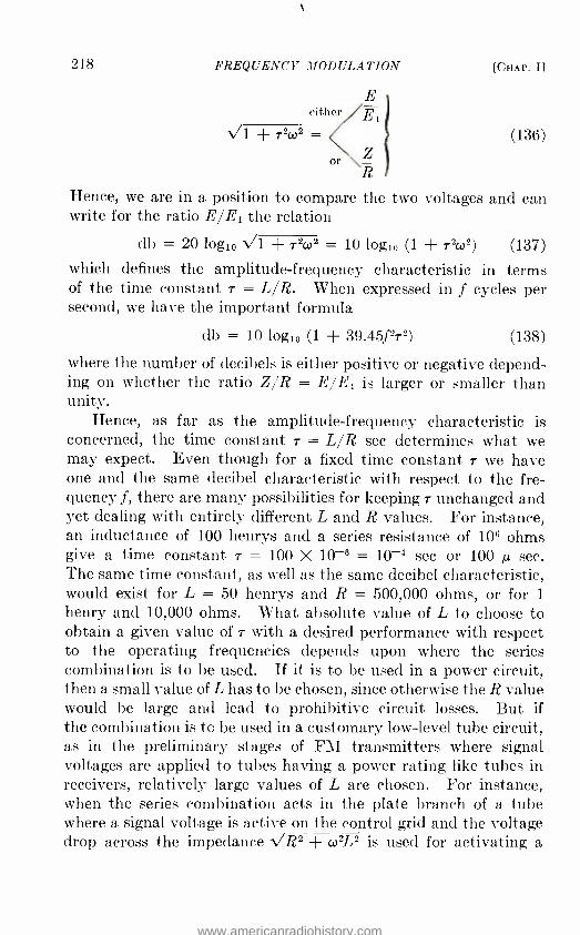
218 FREQUENCY MODULATION [CHAP. II
either
/1 + T2w2 =
or R
Hence, we are in a position to compare the two voltages and can write for the ratio E /E1 the relation
db = 20 logio /1 + 7-2w2 = 10 logro (1
(136)
+ 7.2(.02) (137)
which defines the amplitude- frequency characteristic in terms of the time constant T = L /R. When expressed in f cycles per second, we have the important formula
db = 10 logro (1 + 39.45f2T2) (138)
where the number of decibels is either positive or negative depend- ing on whether the ratio Z/R = E /E1 is larger or smaller than unity.
Hence, as far as the amplitude- frequency characteristic is concerned, the time constant T = L/R sec determines what we may expect. Even though for a fixed time constant T we have one and the same decibel characteristic with respect to the fre- quency f, there are many possibilities for keeping T unchanged and yet dealing with entirely different L and R values. For instance, an inductance of 100 henrys and a series resistance of 106 ohms give a time constant T = 100 X 10 -6 = 10 -4 sec or 100 ,u sec. The same time constant, as well as the same decibel characteristic, would exist for L = 50 henrys and R = 500,000 ohms, or for 1
henry and 10,000 ohms. What absolute value of L to choose to obtain a given value of T with a desired performance with respect to the operating frequencies depends upon where the series combination is to be used. If it is to be used in a power circuit, then a small value of L has to be chosen, since otherwise the R value would be large and lead to prohibitive circuit losses. But if the combination is to be used in a customary low -level tube circuit, as in the preliminary stages of FM transmitters where signal voltages are applied to tubes having a power rating like tubes in receivers, relatively large values of L are chosen. For instance, when the series combination acts in the plate branch of a tube where a signal voltage is active on the control grid and the voltage drop across the impedance /R2 + w2L2 is used for activating a
www.americanradiohistory.com

SEC. 40] AUXILIARY APPARATUS 219
grid of a succeeding tube, it must be realized that dynamically this combination is also across the grid- cathode gap of the suc- ceeding tube, even though an isolation condenser is employed between the stages. Since for the low- frequency range, say 25 cycles per second, R is effective essentially only in the square - root value, this resistance must be high in order to cause sufficient voltage drop on the grid. Hence, a value of about 1 megohm seems suitable. But this requires for a fixed T value, a large value for L also. In a similar way, if the series combination is to be used
e,,,cos Z L : Aúdio
frequency _ Ec .. amplifier
Outputaudió voltage from dscrimina3or
R First audit stage
(a) ACCENTUATOR (b) DE-ACCENTUATOR (in FM transmitter) (in FM receiver)
FIG. 68.- Networks for audio -frequency preemphasis and audio -frequency deemphasis in the upper audio -frequency range of signal currents.
directly in the input side of a tube as in Fig. 68a, then the voltage drop across the inductance drives the grid and we have to use sufficient inductance to cause a desired frequency accentuation in the upper a -f range. This will be brought out in more detail in Sec. 41.
When we deal with a series combination of a condenser C and an ohmic resistance R, we have the impedance Z = -VR2 + 1 /(cwC)2
and in terms of the time constant T = CR sec, the expression
R-V1+w2T 2 = pR
(139)
For an effective voltage E across the series combination, a voltage drop El across R due to the current flow I, and a voltage drop E2 across C, we have
pEi
qI C
(140)
www.americanradiohistory.com

220 FREQUENCY MODULATION [CHAP. II
Hence, if we compare E and E1, we have
db = 20 logro R
= 20 logro p
or
(141)
db = 10 logio 1 1 + W
2 T 2) (142) \ But quite often we utilize the condenser voltage I /wC for causing hie frequency characteristic and we require then the ratio E2 /E,
hick would lead to negative decibel values. If expressed as E /E2, we obtain the answer in positive decibels. By dividing the second expression of Eq. (139) by w on each side, we finally obtain for the comparison of E against E2
db = 20 logio E2
= 20 log10 (wCZ) = 20 logio (qw)
db = 20 logio = 10 logio (1 + (.027-2)
= 10 logio (1 + 39.45f27-2) (143)
This is apparently the same expression obtained in Eq. (138), but with the difference that the time constant is now T = CR sec and we utilize the reactive drop E2 across the condenser C for causing the frequency characteristic. The frequency f in this formula is again in cycles per second.
If we also use in Fig. 68a the reactance drop E2 that exists across L, we can find the solution by multiplying the second expression of Eq. (134) on each side by w and taking the ratio Z /wL = E /E2. We then have
(-co) db = 20 logro (2) = 20 logro = 20 logro
V where m = - T 2 + w2. Hence
db = 20 logio (É) = 10 logio (1 + T2) (144)
This result looks like the result of Eq. (142), but we have to realize that we are dealing now with the inductive drop E2 and with a time constant T = L/R sec. We note, therefore, that the decibel expressions in terms of time constants are, so to speak, interchangeable when having a resistor R in series with an induct- ance L, instead of in series with a capacitance C.
www.americanradiohistory.com

SEC. 41] AUXILIARY APPARATUS 221
All cases just treated are of importance when dealing with corrective networks for a -f preemphasis and deemphasis and will be applied now.
41. Networks for Audio -frequency Accentuation and Deaccen- tuation.- Networks for a -f accentuation and deaccentuation are also known as circuits for a -f preemphasis and deemphasis, respec- tively. The former network is used in the FM transmitter and requires, therefore, the latter network in an FM receiver in order to offset the preemphasis action so that sounds with the correct relative amplitudes in the a -f spectrum will be heard. The reason for using such networks is that most disturbing a -f noise in a
transmitter, irrespective of whether modulated in amplitude, frequency, or phase, seems to lie somewhere between 5 and 15 kc. Since the useful relative amplitudes of the desired a -f signals are generally small in the upper a -f range, preaccentuation is provided in the upper a -f range for the desired signal currents, with respect to desired signal currents in the lower a -f range. Electrically, such preaccentuation can be accomplished with simple circuit ele- ments as well as the equivalent deaccentuation in the FM receiver.
Figure 68 shows such networks, where the network used in the transmitter consists of a suitable resistance R in series with a suitable inductive reactance wL; in the FM receiver a suitable resistance R in series with a suitable reactance 1 /wC is employed. In each case the reactance drop is applied to the grid branch of a class A amplifier and the respective input voltages act across the series combination of the correcting networks. When no other correcting network, such as a 1/f corrector, is employed in a transmitter, then this correcting network precedes the modulator; i.e., the output of the tube of Fig. 68a causes the signal voltage which affects the frequency modulator. If additional stages of a -f amplification are employed after the microphone, then the correcting network should be located right after the sound pickup. The preaccentuator can also be used in the plate branch of a tube as in the transmitter of the General Electric Company (Fig. 73). The R2, L2 network then acts as the accentuator and the effective voltage variations across the impedance Z2 = Á/R22 (wL2) 2 cause preemphasized amplitudes in the upper a -f range and are applied to a single quadrature tube.
Accentuators as well as deaccentuators are apparatus where the time constant r has to be chosen so as to obtain the correct
www.americanradiohistory.com

r= R=/O0psec. R2
[ III IIII
222 FREQUENCY MODULATION [CRAP. II
desired amplitude- frequency characteristic. A time constant of T = loo A sec is considered good engineering practice. Hence, for the case of the accentuator R2, L2 shown in Fig. 73, we have T = L2 /R2 = 100 ,u sec and we obtain the transmission charac- teristic of Fig. 69 by means of Eq. (138). In Fig. 73 it will be noted that the voltage drop across both L2 and R2 is applied toward the grid of the reactance tube. Hence, a high impedance branch has to be chosen so that the grid voltages will be appreciable. Choosing L2 = 100 henrys and R2 equal to 1 megohm yields the
30
25
20 0 X15
óI0
5
0
R2 is impedance at zero frequency
db =20 Zz /0 9'io Rz
Usefu /audió frequency range
2 ó 0 000 O 000 N MA ó Cycles per second
Fin. 69.- Response characteristic in decibels.
000 008 M
0 00 0 00 O 00 000 O 00 000 Ó L.n'Ó 0-0'0 0
ó
requirement T = 100/106 = 100 A sec, and it is, therefore, only necessary to use in the receiver a deemphasizer which also has a time constant of 100 ,u sec. The ratio of the effective impedance Z2 to the series resistance R2 is used in obtaining the decibel characteristic of Fig. 69, since the L2, R2 emphasizer in the plate circuit of Fig. 73 applies its series terminal voltage toward the modulator grid. As far as the audio frequency is concerned, the voltage drop across resistance R2 is essentially responsible for the lower a -f range; at the upper a -f range the inductive drop accounts essentially for the applied a -f voltage. Hence, comparing the impedance Z2 = V/R2 + (wL2)2 at any frequency with the lowest impedance which can ever occur, and which is equal to R2, must give the proper frequency characteristic for the entire audio range.
Figures 70a and b show CR type a -f accentuators and deaccen- tuators each having a time constant of 100 ,u sec. In the FM
www.americanradiohistory.com

SEC. 42] AUXILIARY APPARATUS 223
transmitter of the RCA shown in Fig. 35, the drop across a series combination of an inductance L and a resistance R is used as an a -f preaccentuator. It will be noted that an adjustment is provided for bringing about the best upper a -f emphasis. We note that an a -f response flat within 2 db from the value of 1,000 cycles per second can be expected from 50 to 15,000 cycles per second.
r =CR =100,4 sec.
C= 000/Fcf
I I Class-A
To500ohm!
frequency L R=IOOk e discriminalor source Accentuator fix- output
(a) -In transmitter
r =/00,4 sec.
R=100k
C= 0001/4
17- (0e- accentualor
(b) -in FM receiver
Class-A amp/lifer
Fm. 70.- Accentuator and deaccentuator for a time constant t = 100 microseconds.
This flatness requires, of course, that a deemphasizer of the same time constant be employed in the FM receiver.
42. Networks for Producing Inverse Frequency Effects. -As has been discussed at several places in this text, for indirect FM we have to apply to the balanced amplitude modulator not a voltage en,, cos wt but a voltage that is proportional to (em /f) cos wt, in order to cause subsequent phase swings that are proportional to SO /f instead of to AO as in customary PM. Figure 71 shows the
R=200k
In plate of triode Imcos cut
-- ea
C=0.2,4f
Audio amplifier class A
eg = f, cos wt. dt WC sin wt =k f sin cot
proportional to 1/f Fia. 71.- Network for producing inverse audio- frequency effect.
predistorter that produces the inverse frequency effect. This is the predistorter in the block diagram of the Armstrong transmitter shown in Fig. 33. It is connected between the line amplifier and the a -f preaccentuator. The 1/f network consists of a high resistance R in series with a condenser C, the reactance of the condenser being relatively small at the lowest desired signal frequency f in comparison with the R value. R = 200,000 ohms and C = 0.2 /If are accepted values giving a time constant T
www.americanradiohistory.com

224 FREQUENCY MODULATION [CHAP. II
CR = 0.04 sec. The decibel characteristic for comparison of the total applied signal frequency voltage to the corresponding condenser voltage can be expressed by means of Eq. (143). If the above value for the time constant T is inserted, we have db = 10 loglo (1 + O.O361f2) where f is in cycles per second.
Apparent PM sets in with a modulation index Al
F=200kco-11--. Piezo
oscillator o
Unmodulated carrier
f- network R C 'L .J
B3
To frequency multipliers
T i 1 _ B2
' jb (ampG'fiédphase- shifted modu/anon
product)
Modulation product 90 °shifted in
phase
Input of audio
frequency f 72.- Application of an inverse audio- frequency network.
The derivation in Fig. 71 shows that the voltage applied to the amplifier is proportional to thé amplitude im and is inversely proportional to the signal frequency f where k is the constant of proportionality. When the a -f accentuator is omitted we have then the circuit of Fig. 72. We note that when the modulation product b, which was shifted in phase by 90 deg, is combined with the unmodulated carrier component a, we have a + jb with a maximum phase swing which is now AO /f and this has all the features of the value OF /f previously obtained for direct FM.
www.americanradiohistory.com

SEc. 42] AUXILIARY APPARATUS 225
When a PM is changed into AM by a frequency discriminator, the translation is due to the equivalent frequency swing f AO cos cot.
The same network as shown in Fig. 71 can be used after the frequency discriminator in order to cancel the f effect in the equivalent maximum frequency swing f AO. A customary FM receiver with an additional 200,000 -ohm resistor and a 0.2 -1.f condenser will then work also on PM waves.
www.americanradiohistory.com

CHAPTER III
TRANSMITTERS FOR FREQUENCY MODULATION
Unlike the usual practice in AM transmitters, most of the essential operations in FM transmitters are accomplished at low power levels, as a matter of fact with power levels as customary in receiver tubes. We may, therefore, divide a high -power FM transmitter into three essential parts: one part that causes primary or master frequency modulation, a second part that deals with frequency multiplication, and a third part that involves power step -up. For direct FM, the primary FM would take place about a center frequency which is either one -eighth or one -ninth of the center frequency of the radiated electromagnetic FM wave. An eightfold frequency multiplication, for instance, is employed in the Western Electric FM transmitter, and a nine- fold frequency multiplication is present -day practice in the General Electric and the RCA FM transmitters. Hence, with present -day FM allocations, the Western Electric transmitter would use primary or master FM about a center frequency of approximately 5 Mc /sec.
The second part of an FM transmitter deals with the frequency multiplication of the primary FM in the case of direct FM. For indirect FM, as used in the well -known Armstrong system, a very large order of frequency deviation multiplication is required; as a matter of fact, so large that the ratio of the final frequency deviation to primary frequency deviation is much larger than the ratio of the final center frequency to the primary center frequency.
The third part of the FM transmitter involves a mere power step -up. It may, therefore, be said that a 250 -watt FM trans- mitter is more or less the same as the 250 -watt transmitter section in a 50 -kw F \I transmitter.
43. FM Transmitters. -With respect to the above statements a 1 -kw FM transmitter consists of a 250 -watt transmitter stage which is followed by a final 1 -kw power stage. This final stage could also be a 3 -kw unit. For a 10 -kw FM transmitter, we would have the 250 -watt FM stage followed by an intermediate power
226
www.americanradiohistory.com

SEC. 43] TRANSMITTERS 227
stage of 1 kw which, in turn, drives the final 10-kw output stage. For a 50 -kw transmitter the 250 -watt exciter works into a 3 -kw intermediate power stage and this stage works into the 50 -kw output stage. For still higher output power, we would have after the 250 -watt FM exciter two successive intermediate power stages, one of 1 kw and the other of 10 kw, the latter stage driving the final power stage of, say, 100 kw. Such successive power progressions may not be followed exactly by all manufacturers but is, for instance, the case in present -day General Electric equipment.
Normally, the first power unit, in the above examples the 250 - watt unit, is adjusted to conform to good engineering practice in regard to noise level, frequency stability, and fidelity. In some transmitters inverse feedback is also employed in the last power stage.
The output of the transmitter, when calculated by the indirect method, is 0.6 times the product of the plate voltage and plate current of the last transmitter stage. According to present -day practice, the mean frequency or center frequency of the radiated FM wave must remain within ± 2 kc of the assigned megacycle center frequency. Generally, it may be said that in FIVI trans- mitters the frequency stabilization problem is more difficult from an engineering point of view than it is in AM systems, since in direct FM it is the frequency that is being varied by the modulating current. Even in indirect FM there is some difficulty, though the primary center- frequency source is a stabilized piezo generator. The reason is that in this system another stable reference frequency is employed and the frequency stability of the center frequency of the radiated FM wave is a function of the stability of two inde- pendent piezo standards. Yet, it appears that with the indirect FM system the stability should be equal to, if not better than, systems whose center- frequency stabilization depends on some sort of mechanical or electronic control.
It may be said that the design for low noise level and modula- tion linearity is accomplished better in an FM than in an AM transmitter. This seems to be true also with respect to a -f response. The distribution of the modulation energy in the frequency spectrum seems to be the secret that accounts for the inherent low noise -to- signal ratio in FM work. It cannot be stressed too much that the effectiveness in FM exists on account
www.americanradiohistory.com

228 FREQUENCY MODULATION [CHAP. III
of the Bessel distribution of the many side currents and their relative phase relations. No random distribution of energy will
ever produce such an efficient spread of the modulation energy in the frequency spectrum as does FM.
This is explained in detail in the text and has been proved in many numerical examples. For instance, it was shown that if all significant side currents are added with their actual magni- tudes and correct instantaneous phase relationship, we shall always obtain for the resultant vector a constant length that is
equal to the unmodulated carrier level. But, if we miss some significant side currents, then AM is also superimposed on the desired FM. These statements hold, of course, also for PM energy distributions. Now, random energy distributions have no definite phase relationships; they have also no definite frequencies in the spectrum, and undefined amplitude values. The resultant effect as extracted in the frequency discriminator of a receiver cannot, therefore, be efficient. The reason for this is that fre- quency demodulators are specially designed for reversing the modulation actions caused in a true FM transmitter, and accom- plish, therefore, this task most efficiently.
That we have to use wide -band networks is rather favorable as far as noise suppression is concerned. The useful side currents distribute the FM energy over wide limits, say 100 kc above and 100 kc below the assigned center frequency F. For some FM conditions the frequency spread on each side of the center fre- quency is more than the maximum permissible frequency swing of
AF = ± 75 kc and the circuits are usually designed for a band width of 225 kc. But in the same band width many random noise distributions are spread also, even though due only to sharp input impulses. As amplification takes place in the several i -f stages, the combination of the "erratic" random distributions due to noise and the desired and efficient Bessel distributions due to useful FM would give a very strange picture if it were viewed on the screen of a cathode -ray tube. But this picture is, fortunately, not what the human ear hears, since even with a wide -range a -f
amplifier, say of 225 -kc band width instead of the 30 -kc maximum width for AM, we would still not hear what goes on, say, above 16 kc and below 16 cycles per second. This is because the human ear can perceive sound sensations only between the limits of 16
cycles per second and about 16 kc.
www.americanradiohistory.com

SEC. 431 TRANSMITTERS 229
The frequency discriminator of the receiver recovers the modulation energy due to conversion of FM into AM. Hence, the discriminator characteristic converts the frequency swings OF cos wt, which are never larger than ± 75 kc, into amplitude variations that can never exceed signal frequencies higher than the a -f values of f used in the transmitter. The useful a -f recovery after demodulation of the FM -to -AM translation is, therefore, in the audible- frequency range, which is about 15 kc wide for good
a -f amplifiers. Hence, the recovery of the intelligence or modula- tion is only 15 kc wide. The energy distribution in the entire frequency spectrum is, therefore, just as much "squeezed together" by the FM -to -AM translation of the discriminator as it was
"spread out" in the transmitter when frequency modulation took place. The random noise distributions cannot be Bessel dis-
tributions but are spread out in virtue of the available band width of the transfer networks. Hence, the very opposite occurs since
the cause and the result in case of FM are reversed in case of noise.
This means, in other words, that the band width of the transfer networks has to be designed to accommodate all the significant side currents caused by FM. It also means that the wider the transfer networks have to be designed, the more the energy of an interfering noise can and will spread over the frequency spectrum due to the band width. Since only a 15 -kc width can be recovered after the final amplitude demodulation, not all noise energy will be
recovered in the a -f end. This proves that the discriminator is not efficient at all for modulation spreads due to noise components arriv- ing at the input of the discriminator. It is true that some of these features would also exist if we should use networks in AM reception which are 225 kc wide, so that an a -f frequency recovery of
only 15 -kc width would be effective. Also, here the noise energy would, in many cases, spread itself over the entire 225 -kc width, since this is the property of all wide -band networks, and only the energy components in the audible range could affect the loud speaker. It is, of course, understood that, if the noise distribution over the entire band width has large components in the audible spectrum in comparison with the desired a -f recovery, then the noise will "badly" mask the desired intelligence.
With respect to power measurements, the indirect method mentioned above, by means of the plate voltage and the plate current of the last power stage of the FM transmitter, is probably
www.americanradiohistory.com

230 FREQUENCY MODULATION [CHAP. III
a good procedure if the radiation efficiency from this plate end toward radiation space satisfies the value assumed in the formula given. It is difficult to think of a real reliable method of power measurement at such high frequencies as the 40- to 50 -Mc range and the even higher frequencies around 300 and 350 Mc as used for FM relay transmissions.
Up to about 1 kw of power, we can use incandescent lamps that have insignificant reactance effects. A lamp of such a size should be used that it is lighted to considerable brightness when acting as the load of the FM transmitter to be tested. The brightness is noted with a photometer. Afterward the lamp is brought to the same brightness by a 60 cycles per second current and the cor- responding power read off with a commercial wattmeter. It is true that at frequencies such as are used in the FM range, skin effect causes the filament to carry current only near the surface of the incandescent filament. The error is, however, not serious since the brightness of the incandescent lamp depends only on the actual power dissipated in the filament. It does not matter much whether the dissipation is close to the surface or all over the cross section of the filament. The photometer registers essentially the entire effect as expressed by the radiation from the surface of the filament. It is, however, essential to use a photometer or a photo tube that registers all effects of the heat radiations.
A calorimetric method would be more accurate but much slower. A lamp or some other suitable heat dissipater, which acts essentially as a resistance (dissipater in a tuned load branch), is immersed in a calorimetric liquid. If water is used for the liquid and is made to flow by having an inlet and an outlet, and r is the rate of flow in gallons per minute, and T the centigrade difference between the temperature of the water at the outlet and the temperature at the inlet, then the kilowatt power absorbed by the flowing water is P = 0.263vr.
The transmission -line method, using the line surge impedance, which is a resistance Ro = v'L /C ohms at such frequencies, gives the power as RoI2 if a special ammeter is constructed and used for the determination of the effective current I flowing into the surge impedance experienced at the entrance of a properly terminated line. The termination has to be such that no standing waves exist along it. It seems better to use a diode voltmeter and to compute the power from E2 /Ro.
www.americanradiohistory.com

SEC. 44] TRANSMITTERS 231
44. The Armstrong Indirect FM Transmitter. -Since it was E. H. Armstrong's important engineering developments that paved the way for frequency modulation in broadcasting, it may not be out of place to present first his type of transmitter.
Some of the important theoretical contributions that were made prior to any important engineering applications did not exactly predict great advantages for FM over AM. The reason for this was, perhaps, that general solutions of just one phase, i.e., of FM by itself, without taking the difference between wide -band and narrow -band FM into consideration, did not show any particular advantages for FM. Naturally, any system of modula- tion, if ideally applied, should do the same as any other system of modulation. A modulated current does not realize, if it could, whether it is deformed in amplitude, phase, or in frequency. But when we choose suitable carrier -frequency allocations for which even wide -band transmissions are small in percentage compared with the narrow -band transmissions for customary AM allocations, then the argument of the discussion may be somewhat different. If we also take into consideration that at certain frequency allocations certain noises do not show up as much as
for other allocations and that in virtue of wide -band transmission some of the noise energy when existing can be spread partly into a
frequency region that will not affect the a -f output of a receiver, then we begin to realize that FM, as well as PM, may give better receptions than AM.
It was due to E. H. Armstrong's demonstration of the real merits of FM in his famous paper presented at an IRE meeting in 1935, and to the stirring up of interest in the minds of other engineers who have also contributed to the present art of frequency modulation, that the capabilities of FM transmission were even- tually recognized.
Inasmuch as the individual apparatus used in the Armstrong transmitter has been described already, it is now of interest to learn how it is arranged in a transmitter. It is also of interest to learn what other ingenious means are employed in order to change the very small primary time axis swing modulation into wide -band FM, which behaves as though direct FM were instru- mental in producing the action.
The block diagram of Fig. 33 shows the case for a center fre- quency F 43.2 Mc of the radiated FM wave. A stabilized
www.americanradiohistory.com

232 FREQUENCY MODULATION [CHAP. III
primary frequency F1 = 200 kc is taken from a piezo oscillator and fed first into a buffer amplifier. It then divides itself into two parts. One part feeds into a balanced amplitude modulator, and the other part passes toward a carrier -frequency amplifier. The balanced modulator is affected by a signal current that brings about AM. On account of the predistorter, the signal current has an amplitude that is proportional to im / f instead of to im only. The preaccentuator emphasizes the amplitudes of the signal currents in the upper a -f range, while the line amplifier brings about proper primary signal -level voltage and proper matching. The output of the balanced amplifier is the modulation product with the unmodulated carrier portion suppressed. Hence, the output contains only the side -current pair of respective frequencies F1 ± f.
The output coupling of this modulator is such that the side - band modulation product is shifted in phase by 90 deg, and com- bined with the amplified unmodulated carrier. This results in a PM current with a maximum phase swing of ±M /f. The phase swings are limited to values that never exceed ± 30 deg in order to preserve good linearity. The PM experienced in the succeeding buffer amplifier is, therefore, small and never more than one -twelfth of a single complete h -f cycle of frequency F1. This so- called "PM" has now a modulation index ß = O9/ f. When compared with the modulation index ß = OF /f for direct FM, this shows that even though PM is instrumental in producing the present result we have numerically for the entire a -f or signal -frequency range the same conditions in either case. Hence, in effect, the current in the second buffer amplifier can be taken as an FM cur- rent since the number of significant side currents is exactly the same as if direct FM had been instrumental in producing the modulated output. There is actually an additional feature to this type of FM effect. The feature consists in the fact that the center frequency F1 is fixed, not modulated at all, and yet the number of side currents is as though this frequency were oscillating up and down about F1 with maximum frequency swings of (O9 f)f = OF since, according to Eq. (6), the equivalent frequency swing
for PM is f times the maximum phase swing G9 f. We note, therefore, that for maximum phase swings of O f < 30 deg, or
30/57.3 < 0.524 radian, we have for a signal current of frequency f = 50 cycles per second the corresponding maximum frequency excursions of 0.524 X 50 = 26.2 cycles per second.
www.americanradiohistory.com

SEC. 441 TRANSMITTERS 233
This is a very small frequency excursion even for a carrier frequency as low as F1 = 200 kc. We have to deal, therefore, with a very large frequency multiplication in order to produce the final ±75 -kc frequency excursions. If we assume, for instance, that the largest frequency excursion is ± 25 cycles per second, instead of 26.2 cycles per second, the required deviation fre- quency multiplication would be 75,000/25 = 3,000. Hence, if
cascaded frequency multipliers were used, this degree of multi- plication would also produce a final center frequency of 3,000F1 = 3,000 X 200,000 = 6 X 10$ cycles per second or 600 Mc /sec. This value falls completely out of the present -day carrier frequency allocations for commercial FM. Hence, we have to resort to a
scheme that brings about in the multiplied value of the original small frequency deviation an increase much larger than that in the corresponding center frequency. This is accomplished by insert- ing also a stage of frequency conversion between stages of fre- quency multiplication.
The frequency -conversion principle is well known from the superheterodyne technique. It is based on mixing two currents of different carrier frequencies and utilizing the beat or difference frequency of the respective carrier frequencies as the carrier frequency of the converted output current of the mixer. The only difference that exists here, in comparison with the conversion in customary superheterodyne operation, is that in the latter, one carrier current is modulated in AM and in the present case it is modulated in frequency. Hence, the beat frequency of the converted FM current, when beating with an unmodulated current of oscillator frequency Fo, is now (F3 ± OF3) - Fo in case we have reference only to the maximum frequency swings ± F3 of the current of center frequency F3, which mixes with the piezo current of frequency Fo. Hence, the difference frequency reduces only the center frequency but preserves the magnitude of the frequency excursions ± AF3.
The primary equivalent frequency deviation OF1 is dependent on the signal frequency f since AF1 = 0.524f cycles per second. For a maximum phase swing limitation 9 /f of ± 30 deg or ± 0.524 radian, we have to assume the value of the lowest signal frequency f for which we still expect to obtain full frequency swings of ±75 kc
in the final output current of the transmitter. We found that for 50 cycles per second the deviation OF1 would be 26.2 cycles per second.
www.americanradiohistory.com

234 FREQUENCY MODULATION [CHAP. III
Consulting the block diagram of Fig. 33 we note that we have three groups of frequency multipliers. Each group consists of several stages of frequency multiplication in cascade. The first group multiplies the primary center frequency F1 by 16 and produces the new center frequency F2 = 16F1. The second group causes fourfold frequency multiplication and produces a center frequency of F3 = 4F2. The last group employs a fre- quency multiplication of 48 with an output center frequency F = 48F4. Here it must be understood that F4 is much lower than F3 on account of the center -frequency conversion from center frequency F3 to center frequency F4. The frequency multiplica- tion due to all frequency multipliers is, therefore, 16 X 4 X 48 = 3,072; this must also be the over -all frequency multiplication of the primary frequency swing ±6,F1. As explained above, on account of the center -frequency conversion, the over -all center - frequency increase is less than the increase of the corresponding OF1 swing. As a matter of fact, even though the ratio of the final- frequency swing OF to the original- frequency swing OF1 is a whole number, namely, 3,072, the corresponding center - frequency ratio F /F1 does not have to be a whole number, but happens in this numerical illustration to be so and is 43,200/200 = 216. The reason a whole number is not essential is that in the beat method any difference is possible, just as we can generate currents not only of frequencies that are a whole number when related to the time of 1 sec but also a number like 43.26 cycles per second. This is another desirable feature of this method. We can start out with any convenient primary frequency F1 that looks promising with respect to the corresponding deviation frequency multiplication in order to provide full ± 75 -kc devia- tions in the final center frequency F, and yet the exact value of F can be fractional, i.e., not a whole number.
Since we have found that the over -all deviation -frequency multiplication is AF /AF1 = 3,072 in this particular numerical example, we have a means for finding out what is the lowest audio frequency that, for the adopted 3,072 fold multiplication, results in full ± 75 -kc swings in the radiated electromagnetic wave without exceeding maximum phase swings of ± 30 deg in the primary PM. We find then 75,000/3,072 = 24.4 cycles per second for OF1. This means that for audio frequencies below 24.4 '0.524 = 46.6 cycles per second we cannot expect to obtain
www.americanradiohistory.com

SEC. 45] TRANSMITTERS 235
full frequency modulation. It is true that this puts a limitation to this system, but it does not seem serious. Audio frequencies in this neighborhood, and below it, are not always desired since they are in the region of "hum" frequencies, which should be avoided anyhow. That a large number of tubes of the receiver type are required and that careful shielding is necessary should be understood. But this has been successfully taken care of from an engineering point of view.
Since the primary phase swing is AO, f in the original PM, we note that the upper limit of ±30 deg can be kept correct only if the 1 /f effect in SO /f is properly compensated. Otherwise the maximum desired phase swing of ±30 deg in case of the loudest signal transmissions would fall off toward larger f values. The a -f accentuator will take care of this, since it causes larger i,,
amplitudes of the modulating currents toward the higher audio frequencies.
It will be noted that stages of power amplification follow the arrangement shown in Fig. 33. They have to be designed the same way as for direct FM and for band widths of about 225 kc.
45. The FM Transmitter of the General Electric Company. The General Electric Company's FM transmitter, shown in Fig. 73, is based on direct FM; i.e., the primary center frequency F1,
which is in this case not stabilized or "stiff," is varied about its F1
value. An ordinary tube oscillator having a characteristic C, L network brings about primary FM in conjunction with a reactance - tube modulator. The primary center frequency F1 is, on account of the application of only one quadrature tube, due to C, L as well as to a fixed Ci injection in multiple with C. This is because the voltage of the high frequency applied to the grid of the modu- lator tube is leading the tank voltage of the oscillator by 90 deg. Since the quadrature tube can cause considerable linear frequency swings about the primary center frequency F1, only a ninefold deviation frequency multiplication is required. It is, therefore, possible to use two cascaded -frequency triplers in order to obtain ninefold center -frequency multiplication as well. Hence, if the primary maximum -frequency excursions are ±.6,F1, we have in the antenna current of the transmitter an FM of center frequency F = 9F1 and the corresponding frequency swings OF cos wt = 9 OF1 cos wt.
www.americanradiohistory.com

236 FREQUENCY UENCY MODULATION [CHAP. III
Inasmuch as in such a system ordinary tube oscillators have to be used in order to deviate the oscillation frequency freely, it is necessary to stabilize the center frequency of the radiated FM wave. This is accomplished with a great resolving power by means of frequency conversion and a frequency discriminator for affecting the fixed bias of the modulator tube. The frequency conversion takes place in the mixer tube whose output is tuned to
Reactance modulator /853
Primary 6J5 F. oscillator
dF
C/R, phase shifter
Audio bj ka ampl.s
6SJ7-
Osc.grid choke
CL determines ose. frequency 4.8
d Feedback to (vol/ageregulated) 00 lower FM
noise level 6/16
9f =F
Buffer F lst 3f 2nd.I Power amp, - tripler -.- tripler H ampl.
Osc. plate inductance
Osc. plate choke Ft= 9F, +94f cos rut
= Ft/If-cos wt
Fb=F 3Fo
Anlennax
Power amp!
9.F =F 94F =4F
Feedback for freq.' stahi /i- 9F zation
Mixer
R2L2 pre -emphasis network
C4 discriminator r -f by pass
0000
Discriminator for automatic center frequency control
Relay RF choke
Prevents premature ' application
To plate of voltage contactor
R3C3 filter to allow passage only of corrective voltages of f smaller than the lowest signal f
Fo
HFrequency tripler GL /6/4
Piero . oscillator Fo
GL /6/4
11,
0....._ GL /6/4
- -Acts also as a //mite,
= F
3F0
Fb= 95-3 F0
/l- attenuator 5 goal f "a "path corrects frequency drifts input
"b " path causes corrected signal f feed
Fiu. 73.- Essential sections of the FM transmitter of the General Electric Company.
a frequency Fb much lower than the final center frequency F = 9F1. This is done by combining in this tube a small portion of the useful FM current of instantaneous carrier frequency 9(F1 + AF1 cos wt) with an unmodulated current of frequency 3F0, where Fo is the primary stabilized frequency of a piezo oscillator. The out- put of the mixer or frequency converter has then an instan- taneous intermediate frequency of 9(F1 + OF1 cos wt) - 3F0, which is also F + AF cos wt - 3F0. Hence, the final frequency variation AF cos wt is preserved, and the new center frequency F - 3F0 is many times smaller than the center frequency F of the
www.americanradiohistory.com

SEC. 45] TRANSMITTERS 237
radiated wave and several times smaller than the primary center frequency F1 = 1/[6.28 -V(C + Ci)L1 of the master or primary FM oscillator.
We have, for instance, for a carrier frequency assignment of F = 47.7 Mc, a primary center frequency of F1 = 47.7/9 = 5.3 Mc, and a beat frequency Fb = F - 3F0 = 1 Mc, any center - frequency drifts d of the frequency F being preserved in the output current of the mixer. The percentage drift in the final FM current is much smaller than the corresponding off -drift in the beat cur- rent which is applied to the frequency discriminator. Hence, very small center -frequency drifts in the antenna current will greatly affect the discriminator. The discriminator would, for the foregoing numerical example, be tuned to 1 Mc /sec and would, therefore, be so balanced that at this instantaneous carrier fre- quency of 1 Mc no output voltage is possible. Hence, the sta- bilized piezo frequency Fo is so chosen that 9 X 5.3 - 3F0 = 1 Mc, or Fo = 46.7/3 Mc /sec.
According to the theory of the discriminator, for any other carrier -frequency values that are not exactly equal to the assigned center frequency F = 47.7 Mc we obtain either a positive or a negative output voltage on the discriminator. This is because the balance of this apparatus is based on a 1 -Mc tuning, which can prevail only when F is exactly 47.7 Mc. For any off balance of the discriminator, a corresponding direct current will flow along path a in Fig. 73 and will affect the fixed negative bias of the modulator tube. This affects the g value of this tube and conse- quently the magnitude of the injected capacitance Ci, which adds to the value C of the oscillator. If, therefore, the discriminator is so connected toward the grid of the modulator tube as to cause a decrease in the mutual conductance gm when the center fre- quency F of the antenna current drifts toward a lower carrier frequency value, then the fixed Ci injection will also be lowered, since the injected leading i, current from the modulator is lowered. The result is that the primary center frequency F1 must increase its value correspondingly. In turn, also 9F1 will correspondingly increase and can be made just to compensate the frequency drift. Exactly the opposite occurs when the center frequency F drifts toward a higher value and causes an increase of the g,,, value of the modulator tube. A larger Ci value is, therefore, injected in parallel with the capacitance C of the oscillator and the value of F1
www.americanradiohistory.com

238 FREQUENCY MODULATION [CHAP. III
is increased until the correct primary center frequency is obtained. The corresponding effect in the 9F1 action will then compensate the frequency drift d in the center frequency F, which caused the discriminator to operate. We have, therefore, an "electronic" automatic center -frequency control.
There is another provision made in connection with the center - frequency regulation. From Fig. 73 it is seen that along path L
the signal current, which brings about the useful FM in the primary carrier frequency, is also active. Hence, in the instan- taneous intermediate frequency, which is applied from the mixer to the frequency discriminator, we shall also pass on the demodu- lated FM in terms of audio currents. If it were not for the C3R3 filter, which passes to ground any appreciable audio currents that are higher than the lowest signal frequency f of interest, the direct current along path a would have also audio currents flowing along the same path. These currents would more or less cancel the useful FM in the primary FM source. If this C3R3 filter by- passes, for instance, all audio currents above 40 cycles per second, the grid of the modulator tube will experience only super- imposed biasing effects which are essential in the automatic center -frequency stabilization.
Figure 73, as well as the block diagram of Fig. 74, shows other details in the transmitter. The voltmeter E connected across the output branch of the frequency discriminator indicates directly the magnitude of any frequency drifts since a linear relation pre- vails between output volts and the change in the instantaneous beat frequency Fb = Ft - 3F0. The AF cos wt variations in the value of Ft are about the center frequency F of the output current of the transmitter. As far as the direct voltage indicated by the voltmeter E is concerned, it is in linear relationship with respect to the difference frequency F - 3F0 since the voltmeter action is based on a small direct -current flow and the deflection indicates the average effect. In the General Electric transmitter, provision for a less sensitive scale for the E meter is made so that the meter can also be used when tuning up the transmitter. Large center - frequency discrepancies are then possible, which would give con- siderable output voltages on the discriminator.
All other details in Figs. 73 and 74 are self -evident. The a -f amplifier, which contains the preaccentuator R2L2 in the plate branch, serves primarily for obtaining preemphasis in the upper
www.americanradiohistory.com

Am 451 TRANSMITTERS 239
0
/\
5
/Ç Æ
A §
d\
w
k Ñ
e
:
/ §
2 i \ 2 {f s y 2 2(} 7} .4.-- 4.. »* f f §\ 2 \§ > , 3a k[ }6
7aw §k RH/)
/)\/ uAe
www.americanradiohistory.com

240 FREQUENCY MODULATION [CHAP. III
a -f range. The modulation monitor or indicator shown in Fig. 74 is based on the combined action of both FM current and audio current, the latter coming from the output branch of the dis- criminator. It gives, therefore, indications that can be directly expressed in terms of OF swings. Since swings of ± 75 kc are taken as the full permissible modulation, any correspondingly smaller swings give less than full deflections. The piezo oscil- lator of standard reference frequency Fo is self -contained; i.e.,
its supply power as well as the power needed for automatic tem- perature correction are independent of all other voltage supplies. Automatic relay action is also provided in order to avoid severe overloading and premature application of plate voltage.
46. The FM Transmitter of the Radio Corporation of America. The RCA transmitter is likewise based on direct FM and uses electronic center -frequency control as well as a reactance tube modulator. The wiring diagram is shown in Fig. 35. On account of a reactance modulation, we obtain again considerable primary FM, i.e., large frequency excursions that have a linear relationship with respect to the signal- frequency voltage that causes FM. Hence, only ninefold center- as well as deviation- frequency multi- plication is employed. An electron- coupled primary or master oscillator of center frequency F1 is made use of. This oscillator frequency would be 5.3 Mc for a frequency allocation F = 47.7 Mc, since F = 9F1. The oscillator tube is an RCA 807 tube. Two such tubes are also used in the reactance modulator with their plates connected in parallel and across the tank of the oscillator. The modulator grids are supplied with r -f voltage from the oscil- lator, not by direct connection but inductively. Since these grids are driven in push -pull, we have a phase difference of 180 deg from grid to grid, but 90 deg out of phase with respect to the tank voltage E of the oscillator. It will be noted that the phase of the h -f currents in the plate circuits of the modulator tubes are con- trolled by the grid tank. The link coupling and the adjustment are so made that the h -f currents are exactly 90 deg out of phase with respect to the tank voltage E. The two modulator output branches look, therefore, to the plate tank of the oscillator tube like reactive loads, the degree of the injected reactance depending on what happens in the respective grid branches of the modulator tubes. In absence of signal- frequency voltages on the modula- tor grids, the modulator tubes draw equal and oppositely phased
www.americanradiohistory.com

SEC. 47J TRANSMITTERS 241
currents and the injected reactance effects cancel. But, as soon as the signal voltage of frequency f interferes with such a balance, one modulator tube will draw more current and the other modula- tor tube less current. This causes an effective positive and negative reactance across the oscillator tank. We have, there- fore, a differential modulator with twice the frequency -swing ability found in one modulator tube only. Two modulator tubes give besides the advantage that circuit irregularities can be canceled out.
It will be noted that a Crosby type of frequency discriminator is employed for the center -frequency stabilization in order to keep the mean frequency within about 0.0025 per cent of the assigned value. A separate piezo source of stabilized frequency F affects one grid of a mixer tube; the other grid is supplied with energy from the RCA 807 amplifier, which follows the primary oscillator of center frequency F1. For this particular numerical example the plate branch of the mixer is tuned to a difference frequency Fo - F, = 6.3 - 5.3 or 1 Mc sec. The output of the mixer is then coupled to the 6H6 rectifier tube through a discriminator circuit. The direct current of this rectifier is, in turn, fed into the grid branches of the two modulator tubes in order to provide a differential correction bias. Also, in this transmitter no output voltage is obtained from the discriminator when the instantaneous heat. frequency is exactly 1 Mc. But when the primary oscillator frequency F, drifts, a. differential voltage will result on the respec- tive modulator grids and tend to counteract, the frequency drift. The control ratio is such that, the net frequency change is only a very small fraction of the change that would have resulted if the center frequency F1 were not being corrected.
A 6J5 tube or its equivalent, not shown in Fig. 35, is also used in the interlock circuit which is so arranged that failure of any component in the automatic- frequency control unit actuates a relay. This can be used either to take the transmitter off the air or to sound a bell or to do both. The R, L branch acts again as an a -f preaccentuator.
47. The FM Transmitter of the Western Electric Company. - The FM transmitter of the Western Electric Company also produces direct FBI by means of a balanced reactance tube. Unlike the RCA and the General Electric transmitters, we note from the block diagram of Fig. 34 that only eightfold center-
www.americanradiohistory.com

SEC. 47] TRANSMITTERS 243
frequency multiplication, as well as deviation frequency multipli- cation, is employed in order to obtain the final wide -band FM. Automatic center -frequency control is not electronic, but is electromechanically accomplished. It requires several stages of cascaded frequency division.
For a frequency allocation of 46.5 Mc the primary center frequency F1 would be 5.8125 Mc. For the largest permissible frequency excursion of ±75 kc in the radiated wave, we then have a primary frequency excursion of ± 9.375 kc since it must be one -eighth of 75 kc. As Fig. 34 indicates, the center -frequency stabilization is, for this particular numerical case, based on a piezo reference frequency F2 = 5.676269 kc. How these values are arrived at is described in connection with this figure. A synchronous mechanical drive is arranged to affect the respective trimmer condenser settings of the primary oscillator.
The essential wiring diagram is given in Fig. 75. The primary oscillator uses two tubes 1a and lb. The frequency -determining elements are the inductance L1 and the condensers C1 and C2.
The variable portions C2 are mechanically interlocked with a motor drive which varies the settings of C2 until the correct center frequency F1 of the primary oscillator is secured. The correcting motor will, therefore, turn the movable plates of the respective C2
condensers toward more capacitance setting or less capacitance setting, depending on whether the frequency drift in the value of F1 is an increase or a decrease. Direct FM is caused by the two reactance tubes 2a and 2b which inject reactances into the C1C2L1
branch. The plates of these reactance tubes are connected in push -pull across the tuning coil L1. Reactance -tube action takes place, therefore, with double the linearity range with respect tc frequency changes. The grids of the reactance tubes 2 and 2b
are also driven in push -pull by means of a signal voltage due to em cos wt. The bridged T network in the primary branch of the signal frequency circuit is an a -f accentuator. The tuned network of the oscillator tubes 1a and 1b works over a secondary coil L2 into a phase shifter (series coil and shunt condensers) and applies such h -f voltages of the instantaneous primary carrier frequency to the respective control grids of tubes 2a and 2b that the grid voltages are exactly 90 deg out of phase with respect to the voltage E across the tank coil L1.
The control grids of the reactance tubes are, therefore, affected by both, the primary carrier -frequency voltage and the
www.americanradiohistory.com

244 FREQUENCY MODULATION [CHAP. III
frequency voltage. The plates of tubes 2,, and 2h inject generally an impedance across coil LI, which depends on both the signal frequency and the primary carrier -frequency voltages. It is, therefore, essential that the h-f voltage is perfectly constant so that the reactance injections across coil L1 depend only on the magnitude of the signal- frequency voltage. The phase quadrature caused by this phase shifter produces only a weak AJVI effect, which can be observed with a headset across the negative feedback coil L4. A minimum sound will be observed when 90 -deg phase shift prevails. The use of a balanced oscillator, as well as a balanced reactance -tube modulator, gives rise to larger primary AF1 cos wt swings, even though only a small but linear portion of the respective gm characteristic of respective reactance tubes 2a and 2h is being employed.
As was already described in connection with the block diagram of Fig. 34, stabilization of the center frequency is brought about by a mechanical control and is kept in proper step by means of a reference frequency F2 taken from a piezo source. Using again the same numerical values as for Fig. 34 for a frequency assign- ment of F = 46.5 Mc, the primary center frequency F1 of the tube oscillator shown in Fig. 75 is one -eighth of this value or 5.8125 Mc. By means of regenerative ring modulators in cascade, the primary frequency F1 is divided by 1,024, causing the correct reduced center frequency 5.676269 kc. If there exists a slow drift d1 in the primary center frequency F1, it will show up as a reduced drift d1/1,024 in the above -mentioned reduced center frequency. The correction motor and its associated networks are so adjusted that the motor drive will stand still when the reduced center frequency is at its exact value of F1/1,024, i.e., d1 = 0. But it will slowly move in one or the other direction when there exists a drift d1, the direction depending on whether the drift is positive or negative. The motor will keep turning until the trimmer settings C2 cause the correct primary center frequency F1 = 5.8175 Mc. The mechanical control action is then as follows: The reference piezo source produces the correct reduced center frequency F2 = F1/1,024 = 5.676269 kc. The output current of the sub - sequent frequency dividers feeds into two balanced modulators (mixers) using tubes 6(,, 6h, 7,,, and 7h. The piezo source supplies current of the correct reduced center frequency in phase quadrature to each balanced modulator. The exciting fields for the correction
www.americanradiohistory.com

SEC. 48] TRANSMITTERS 2-t 5
motor are in space quadrature. Hence, when there is no drift in the center frequency, the beat currents applied to the windings of the correction mechanism are of zero frequency. The motor drive will, therefore, stand still. As a matter of fact the drive will merely vibrate or "buzz" somewhat owing to the equivalent phase flutters of the useful FM in the subharmonic current flowing to the balanced modulators with tubes 6a,b and 7(ß,b. A correspond- ing beat frequency will, therefore, be produced and the motor drive starts to rotate in a direction depending on the polarity of the fre- quency drift d1 and keeps moving until the proper value of F1 results.
48. FM Signal Generators. -As has been discussed at several places in this text, many tests on FM networks can be made with simple means, i.e., with high -resistance direct voltmeters, ordinary beat -note indicators, milli- and microammeters, and customary AM signal generators. For the manufacturer of FM sets, better equipment should be used so that all operations of a receiver can be tested thoroughly. A signal FM generator will facilitate a checkup of FM receivers. Such a signal source should cover the carrier -frequency range of FM allocations as well as the inter- mediate- frequency range. Since such an FM signal generator can be greatly simplified if the center- frequency stabilization is omitted, certain means have to be provided to keep the center frequency fairly constant after the generator is warmed up. A voltage regulator is then used in the power supply, so that the heater, plate, and screen voltages can be considered as though coming from batteries. This is especially a requirement for the reactance tube.
Figure 76 shows a simplified FM generator,' which incorporates two frequency tripiers; i.e., it is based on ninefold frequency multiplication. If the primary center frequency F1 is chosen as 4.6 Mc, it will cause an output current corresponding to a frequency allocation of F = 9 X 4.6 = 41.4 Mc. The maximum permissible frequency deviation of OF = ±75 kc in the FM output voltage requires that primary linear frequency swings of OF1 = 7% = ± 8.333 kc must be possible with respect to signal -frequency voltages. The band width of the networks before multiplying the instantaneous primary carrier frequency has to he at, least 2 AF1 = 16,666 kc wide. Between the first and second tripler tubes, the
' HOBBS, M., A Low Power Transmitter for Demonstrating FM Receivers, Elec- tronics, January, 1941, p. 20.
www.americanradiohistory.com

246 FREQUENCY MODULATION
r 1
h ti
J --- , cs. ' y
àáá,óo 6QóSe
[CHAP. III
www.americanradiohistory.com

SEC. 48] TRANSMITTERS 247
networks have to have a band width of at least 6 OF1 = 49.998 kc. After the second tripling occurs, a band width of at least 150 kc is required. For good transfer- network design, the band width should be three times the largest permissible frequency swing and should also have a linear phase characteristic with respect to all pass frequencies. The schematic diagram shown in Fig. 76 is self -explanatory since it is a simplified FM transmitter.
It is stressed that when testing FM receivers with such a signal generator, either pure sinusoidal signal frequency voltages of frequency f should be applied across the terminals where the crystal microphone pickup plugs in or a high -grade crystal pick -up should be used in connection with direct sound pickup. This cannot be stressed too strongly since, after all, FM stands for improved a -f fidelity and recordings are just not good enough for testing superior a -f performance.
It will be noted that a single tube is used in the primary oscil- lator as well as in the modulator. A 6J5 tube, or its equivalent, is employed for the oscillator tube, having a suitable gm value. A 6AG7 tube, or its equivalent, is suitable as a modulator tube. Such a tube can also be used in the output stage, which feeds into a low- impedance transmission line in order to provide the proper termination toward the input side of FM receivers. Such receivers are usually designed for dipole reception where we have about 100 ohms as a termination. In the tripler stages and for the first and the last tube of the a -f preamplifier 1852 tubes or their equiva- lent are used. The modulator tube and the 1852's are mounted on cushion sockets and are especially selected from a group of such tubes in order to avoid microphonicness. The output voltage for the indicated termination is between 5 and 10 mv. This is approximately the value experienced in FM receivers in a metro- politan area.
It will be noted that the a -f accentuator is made up of a 20- ,uf
condenser in parallel with a 5- megohm resistor, and the combina- tion is in series with a 50- 000 -ohm resistor. This accentuator acts toward the grid branch of the last audio stage of the preamplifier. With only a 20 -µµf condenser and a 5- megohm resistor, we shall have a time constant of exactly 100 sec which is generally accepted as good practice. Having also a 50,000 -ohm resistor in series with this predistorting network, we have a means for adjusting the over -all frequency characteristic.
www.americanradiohistory.com

248 FREQUENCY MODULATION [CHAP. III
The last 1852 tube of the a -f preamplifier uses a low external plate resistance as is customary in television amplifiers. Such a plate loading will preserve the effectiveness of the audio amplitudes of the higher frequencies, which otherwise would be greatly decreased owing to the capacitance in the modulator grid branch. It will be seen that the 13.8 -Mc coupling between the output of the first tripler and the input of the second tripler is obtained by means of a 1,000 -µµf condenser joining the two fixed condensers. A certain over -coupling between the two networks also has to be provided in order to obtain the proper band width, which should be somewhat greater than 50 kc. Brass cores in the respective coupling coils are used for tuning to 13.8 Mc for the alignment of
this band -pass coupling. Inasmuch as the output branch of the second tripler has a center frequency as high as 41.4 Mc, the inductance effects of the leads are too pronounced to make it advisable to use condenser interstage coupling. Hence, the primary and secondary coils of the interstage transformer are wound on a common insulating core about ;4 in. apart so that the needed inductive over -coupling prevails. Tuning is accom- plished by 25 -µµf trimmer condensers, which are also shunted by resistors of 25,000 ohms in order to flatten out the double hump. An output terminal for applying a -f voltages to the vertical deflection plates of a cathode -ray tube is also provided, so that the wave form can be examined.
www.americanradiohistory.com

CHAPTER IV
RECEIVERS FOR FREQUENCY- MODULATED CURRENTS
In many respects FM receivers are similar to AM super- heterodyne receivers. For instance, the received antenna current is first converted into a suitable intermediate frequency and then several stages of i -f amplification are used. Then a frequency demodulator, instead of an amplitude demodulator, is used and followed by customary high- fidelity a -f amplification. The audio amplifier should be flat from 50 to 15,000 cycles per second within 2 db with respect to the amplitude at 1,000 cycles per second. On account of the many significant side currents, much wider band -pass networks have to be used in all the h -f stages, including the input side of the frequency demodulator. This is, however, no longer a difficult engineering problem, especially for present - day FM allocations. As far as the operation of such a receiver is concerned, it is not any more involved than is the operation of an AM receiver.
49. FM Receivers. -Present -day FM receivers are designed with a sensitivity to respond to voltages as low as 10 to 40 µv. The field intensity contour required by the FCC is 50 µv / m. We note, therefore, that high -gain tubes have to be used, so that sufficient amplitude will be available for amplitude limitation and still leave an i -f carrier level after limitation such that good a -f recovery is possible. Generally, the signal -to -noise ratio of con- verter tubes is not exactly good in the 40- to 50 -Mc band of carrier frequencies. For certain receiver locations it may be desirable to obtain as much gain as possible before frequency conversion into the intermediate frequency takes place. Such increased gains can be obtained by using an antenna gain, as well as by a gain in the radio -frequency stage. Antenna gains as high as about 5 to 10 are possible, as well as a gain of this order of
magnitude of h -f stage ahead of the mixer causing the inter- mediate frequency.
An 1853 tube or its equivalent seems better than an 1852 tube for the h -f amplifier stage, since it can be used with a variable
249
www.americanradiohistory.com

250 FREQUENCY MODULATION [CHAP. TV
amplification control. Such a control is of benefit when received voltages of more than about 50 µv reach the input side of the FM receiver. Reception of the signal at several positions of the dial may occur unless the h -f gain is reduced. If an 1852, or its equivalent, is used as a converter (g, = 3,000 for a 6,000 -ohm loading), with a gain of about 18, good conversion is obtained with peak oscillator voltages of 2 volts or more. For the FM alloca- tions between 42.1 and 49.9 Mc, the grid current is then about 1µa. A 6SA7 tube, or its equivalent, seems especially good as a mixer tube because, even if no automatic volume control is used, the applied antenna voltage can vary from 1 to 105 µv without causing appreciable drifts in the oscillator frequency.
With respect to intermediate frequencies, ordinary i -f trans- formers, such as are used in AM receivers (460 kc), have been used in FM receivers when quality and image response were of no concern. Intermediate -frequency stages with 1.7 Mc for the intermediate center frequency have also been used. But present - day practice employs mostly i -f center frequencies of 4.3 Mc and sometimes as high as 5.25 Mc. Such higher i -f frequencies move all image- response signals from the FM receptions in the 42.1 to 49.9 -Mc band beyond the tuning range. Therefore, the main image frequency interference due to other FM stations is avoided. It is true that oscillator frequencies that occur, say, 4.3 Mc below the center frequency of the tuned -in FM wave, can cause image effects with carriers in the 30- to 40 -Mc band. Fortunately, the image ratio for such carriers will hardly cause audible beat -note interference.
The selectivity of a receiver is generally chosen such that it is about 6 db down at + 75 kc and about 20 db down at + 100 kc from the center frequency. Generally, two i -f stages precede the limiter stage. For one limiter stage the gain is usually about unity. In some designs an 1853 h -f stage is used, followed, for instance, by a 6SA7 mixer stage, which works into two linear i -f amplifier stages. These i -f amplifier stages use, for instance, 1232 tubes. Then two limiter stages follow employing 6J7 tubes. The output of the last limiter feeds into a 6H6- frequency dis- criminator and the remaining portion of the receiver is the same as in high -quality AM receivers. Hence, the demodulator feeds into an a -f deaccentuator before a -f amplification sets in. It is important that each coupling stage be shielded by itself. If this
www.americanradiohistory.com
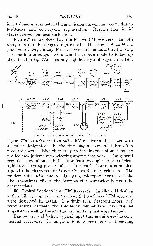
SEC. 50] RECEIVERS 251
is not done, unsymmetrical transmission curves may occur due to feedbacks and consequent regeneration. Regeneration in i -f stages causes nonlinear distortion.
Figure 77 shows block diagrams for two FM receivers. In both designs two limiter stages are provided. This is good engineering practice although many FM receivers are manufactured having but one limiter stage. No attempt has been made to follow up the a -f end in Fig. 77a, since any high -fidelity audio system will do.
\e O\Qo
(a)
s High frequency L. amplifier F-421t0999
Mc
1853 /852
(b)
50 -15000
6S A7 6J 7G 67G cps
6J76 /852 /232 /232 68J7 6SJ 7 6116 6SF8 6/f8 6511'7 681(7 /852 /852 6C5
4.3 4.3 4.3 4.3 4.3 firsf Cusfo ÿ nverter
F'43Mc f=43Mc M f =43Mc
MF= 43Mc
limiter Mc /F-43Mc
limiter Mc frequent
demodulator audio audio
amplifiers
y6SJ7 6K8 6K8 6SJ7 /852 /852 High frequency amplifier
F= 30-40Mc
F Mixer 5Mc Mixer 456kc Jr --- Ft5Mc 5t0456McT456kc -
F ±5Mc 5 ±0.456 Mc
456kc Limiter 456 k
456 k
F±5Mc
Pint) _ )( oscillator
5±0 456
Mc
Pieza% oscillator
6H6
Limiter 456 k
6116 5015000
456 k rrequencyLcps demodulator
6K6K 6CBG Audio 15000 Audio
output - amplifier sta e cps amdsquetch
SO 15000 cps
FIG. 77. -Block diagrams of modern FM receivers.
Figure 77b has reference to a police FM receiver and is shown with all tubes designated. In the first diagram several tubes often used are shown, although it is u.p to the designer of such sets to use his own judgment in selecting appropriate ones. The general remarks made about suitable tube features ought to be sufficient guide for selecting proper tubes. It must be borne in mind that a good tube characteristic is not always the only criterion. The random tube noise due to high gain, microphonicness, and the like, sometimes offsets the features of a somewhat better tube characteristic.
50. Typical Sections in an FM Receiver. -In Chap. II dealing with auxiliary apparatus, many essential portions of FM receivers were described in detail. Discriminators, deaccentuators, and terminations between the frequency demodulator and the a -f amplifier as well as toward the last limiter stage were treated.
Figures 78a and b show typical input tuning units used in com- mercial receivers. In diagram b it is seen how a three -gang
www.americanradiohistory.com

252 FREQUENCY MODULATION [CHAP. IV
condenser is arranged and connected in order to line up the oscillator as well as the other essential variable tuned circuits. A
high frequency amp /ifier 63K7
Antenna
Ik
óoifif 04k ..,. 50k
00//if ---
IFskrge
.--- Ik - - ---T-
1 Q1 °- 1 xtR, I i .--
I / ,/dOlicf - I /' =OQ;,uf 1
L' --- - - ----- -1 Tuning unit-4
[ci/ /attor coil
Three gang condenser-- control
Mixer, coil Y
0..000035,af
6SA .
FirstlFs/age 0.01,ccf I T- - -
To grid of /852
-1300 volts
(a )
To grid I ó I ó
13_
J IF-transformer H
-Tuning
75k 0.0005gf =V 1k I unit
T O.IIk"'
0.0//cf-
,..50 ohms
Ik 0.0005/uf
- '
Ok I
An nna coil
e 02.1.1 A k J
ls/ts,9- L -- - - -J
/ -2 are input terminals of FM receiver leading to a dipole
L7 ,6, -VR /50
Voltage regulator
Fin. 78.- Typical tuning units in FM receivers.
(b)
regulator tube is also incorporated in order to keep any drifts in the oscillator frequency to a minimum.
www.americanradiohistory.com

SEC. 50] RECEIVERS 253
Figure 79a shows an 1852 tube or its equivalent acting as a h -f
amplifier of the voltage induced by a dipole current. It also
shows how the various condensers are ganged up to a common
control. Figure 79b shows an 1853 tube used as a h -f amplifier
and a 6SA7 tube in the converter stage. In such an arrangement we may expect good oscillator stability and can make use of the
variable amplification- factor control of the first tube. It will also
First trans former -r
(a)
High frequency 1852 i stage 6K8
Converter
, 016k =) 60k
0001 f
/
Three gang cordensers6SA7
1853 r 1q
OOOIL- ß k /0.001,uf
/ 0.4k'
005 f
á
Sk
-J 0.0/
(b)
1k
Converter
I L ro
First IFtransformer
0.0ó;u
005/ßf
7ok
+Bof power pack ( +300 volts)
FIG. 79.- Typical input networks of an FM receiver, including high- frequency stage, converter and its outgoing i -f branch.
5k
To grid of first
lOk Famplifier
-+,700 volts
To first
T , 60k i IFamp/ifi'er
+300 volts
be noted that more h -f gain can he expected since this tube is
neutralized as far as the input conductance is concerned. The
neutralization is accomplished by a connection between the grid -
return condenser and the cathode of the 1853 tube. Hence, the
inductive voltage in the leads of the cathode by -pass condenser
neutralizes the voltage across the cathode lead within the tube.
It will also be noted that the coupling between the converter output and the first i -f stage, as well as the interstage i -f coupling (the
latter not shown in this figure), is by means of a capacitance of
about 2,000 µµf common to the 50 -µµf condensers. A certain degree of overcoupling between the two networks is also provided, in order to obtain the desired band width, which should be about 225 kc. At ±75 kc from the 4,300 -kc center -frequency setting,
www.americanradiohistory.com

254 FREQUENCY MODULATION [CHAP. IV
the selectivity is not much more than 6 db down. At ± 100 kc it is not more than about 20 db down. It should be about 20 db down to avoid adjacent channel interference.
It should be understood that in FM receivers the recovered audio output is a function of the time rate of change of the instan- taneous value of the carrier frequency. The percentage of time rate of change is larger for the corresponding center frequency in the i -f stages than it is in the FM current flowing in the receiver antenna. This follows from the fact that the frequency swings in the i -f stages are of the same order of magnitudes as are effec- tive in the received antenna current. But the i -f center frequency is only 4.3 Mc ; it is somewhere between 42.1 and 49.9 Mc in the antenna FM current.
It is essential that all the interstage couplings, including the one between the last i -f stage -the limiter -and the input network of the frequency discriminator, have transfer characteristics that are linear with respect to phase shifts. For nonlinear phase -shift characteristics, even though symmetrical about the center fre- quency, we would obtain amplitude distortion. Fortunately, it is much easier to design linear transfer networks than to design linear tubes. It may be assumed that for a good engineering design the distortion due to a slight nonlinearity is less than about 1 per cent of the peak value of the recovered a -f signal amplitudes.
With only one limiter stage, which is the stage preceding the frequency demodulator, and with linear transfer characteristics up to the discriminator, the gain is mostly due to the stages pre- ceding the limiter. With such low supply voltages as have to be used for amplitude modulation, the gain in the limiter tube itself is only about one and may be only from two to four for two limiter stages. By using suitable high -gain tubes and a high - efficiency converter for causing intermediate frequency, the over -all gain can be driven to the value needed to produce sufficient a -f recovery.
It is also essential that the time constants in the limiter circuits be relatively fast, say only a few microseconds; they should not exceed 3 µsec. Such speedy actions are required in order to keep the effects due to impulse noise away from the discriminator. When, therefore, two limiter stages, as is desirable, are used in the receiver, then the capacitance coupling toward the first limiter
www.americanradiohistory.com

SEC. 50] RECEIVERS 255
grid is made, say, 50 µµf and the grid resistor from grid to ground is made 50,000 ohms. Then we shall have a time constant of
50 X 10 -12 X 5 X 104 = 2.5 µsec, which is sufficient to keep
impulse noises due to automobile ignition fairly well down so that only a very small portion of them will ever reach the plate branch of the first limiter. It can, therefore, affect the discriminator somewhat if only one limiter stage is employed. But if we use
an additional limiter stage with a grid condenser of 50 µµf as in
the first limiter, but with a grid -leak resistor only half as large,
i.e., equal to 25,000 ohms, then the time constant for the grid
input of the second limiter is also only half as large. The resulting value of only 1.25 usec should, no doubt, cut down the remaining ignition interference to next to nothing.
It is because of such cummulative actions that the desirability of using two stages of amplitude limitation cannot be stressed too
much. It is to be hoped that FM receiver engineering will follow
good engineering design and not omit just one tube with a few
circuit elements whose adjustment is not difficult in order to save
economically at the expense of the basic advantage of FM, i.e.,
quality with less interference. Figure 80 shows how two limiter i -f stages are connected
between the i -f stage which has no amplitude limitation and the 6116 frequency discriminator. It also shows how the discrimina- tor terminates into an a -f deaccentuator whose output voltage e
is applied across a 2- megohm potentiometer, which supplies a
suitable a -f driving voltage to a class A amplifier tube. This amplifier tube is the first stage of a -f amplification. All networks following are the same as in customary AM receivers having high -
fidelity audio stages, which are flat within 2 db of the 1,000 cycles
per second value over the entire audio range from 50 to 15,000
cycles per second. In the wiring diagram, the significant time constants are inscribed at the proper places. Essentially these values of time constants should be used, irrespective of whether the same or other tubes are employed. For instance, the deac- centuator ahead of the first audio amplifier tube must use a time constant of 100 y sec since such a time constant is employed in the preaccentuator of FM transmitters. The purpose of the deac- centuator in the receiver is, after all, to offset exactly the frequency emphasis toward the upper a -f range introduced in the transmitter. Even though the amplitude a -f characteristic can be varied by
www.americanradiohistory.com

256 FREQUENCY MODULATION [CHAP. IV
II w &
j Æ \
y
k / 2 . \w o
\ \\ \K *> ex
_2
1
, I)`-- g
\ \| L - 2 f , w ª t w @§ª\ \
2I * :-4
\I |
II / - * ±
fr
L - - i 7\
www.americanradiohistory.com

SEC. 51] RECEIVERS 257
using a small additional control in the deaccentuator, it does not seem wise to use such additional correction in a commercial receiver unless it can be fixed.
51. Characteristic Curves in FM Receivers. -Many of the functions that the different circuit portions have to perform have already been discussed at different places in this text. It is now
of importance to apply such functions to actual circuit conditions In Sec. 50 it was brought out how certain impulse noises can
be reduced, as far as their effects in the discriminator output are
concerned, by employing grid input networks that cause fast actions, i.e., by using networks that have a small time constant.
10,000
° 1000
cIá 100-
c c I
(a)
Selectivity for AM at - 1000 k
000 10,000
1000
10 P2 00
10
1 1 ( 1 1 I I 01
-301 -20 -10 0 10 20 30
- off-resonance +off- resonance Kc.
S1.- Selectivity curves of AM compared with i -f stages used in FM networks.
Generally, circuit actions, if their speed is of interest, are con-
veniently expressed in terms of time functions such as the time constant (consult Sec. 40). This can then be compared with the desired sinusoidal speed actions as well as with the transient speed of certain desired actions; for instance, the actions in case of
television blanking impulses or the perpendicular ascenders of square waves. The time constant can also be compared with undesired actions as ignition and other noise interference.
In ordinary alternating- current applications we know that when a coil with a relatively high natural period feeds, for instance, into a load like the secondary of a h -f output transformer, a good
amplitude- frequency characteristic may be expected. The reason is that the natural period of the output coil is high compared with the period of any sinusoidal components of the resulting output current flowing in the coil. This is actually another way of express ing what happens when dealing directly with time constants. Effective time constants must be used when several networks are
concerned, since it is not always possible just to accumulate
(b)
IT-Selectivity at 43 inc. _- for primary FM stages
at input of the /imiter
000
100 i; v 6
10 °
I rp
01
-300 -200 -100 0 100 200 300 - off-resonance 4- v + off-resonance
Kc.
www.americanradiohistory.com

258 FREQUENCY MODULATION [CHAP. IV
individual time constant effects when there exists appreciable mutual coupling, between the networks, which are reversible.
Figure 81a shows a typical selectivity curve. The ratio of the signal input at somewhat off -resonance to the signal input at resonance, referred to normal output, is plotted against the frequency deviation on each side of the true resonance setting. Figure 81b gives a typical selectivity characteristic in terms of the input voltage with respect to the detuning. The over -all
-80
-300 -200 -100 0 100 200 F +/IF
itc off resonance below input of first limiter Fm. 82.- Decibel characteristic of the over -all selectivity ahead of the amplitude limiter.
selectivity is what counts, and this can be taken only before the first limiter stage since the limiter "clips off" the amplitudes to a constant level. Consequently, constant i -f voltages are impressed on the frequency demodulator. The selectivity characteristic of Fig. 81b, therefore, refers to the FM voltage which acts on the first limiter grid. Figure 82 gives the corresponding typical decibel attenuation characteristic for the over -all i -f selectivity observed at the input of the first limiter. Figure 83 shows how the limiter acts when different magnitudes of frequency swings take place. The knees of these deviation characteristics are points above which the flat portions of the characteristics cause constant discriminator input voltages for increasing FM voltages
300
www.americanradiohistory.com

SEC. 52] RECEIVERS 259
impressed on the input terminals of the FM receiver. It is the
saturated portion of these characteristics that causes the desired
discriminator action. The saturated input voltages have then
the same value as at the output of the last limiter. It is to be
noted that from about 8 µv upward, the useful FM variations are
effective on the discriminator. Below such input voltages, at the
terminals of an FM receiver, random noise, as indicated by the N
characteristic, becomes more or less prominent.
o
-40 -10 0 10 20 30 40 50
Relative FM voltage -input in decibels at the input terminals of a FM receiver
FIG. 83.- Limiter characteristics for different maximum frequency swings.
Useful limiter range AF_ZSkc
;a
% t 25kc. (----\
. -l5kc.
Noise \<.
I l i 1 1 1 1 1
\ .. ' 52. Image Response in FM Systems in Comparison with Such
Responses in AM Systems. -From customary superheterodyne experience we know that in ordinary AM receivers we can classify
five types of interference that result when a local oscillator current
of frequency Fo mixes with a desired received current of frequency
F1 to produce an intermediate frequency Fi. The five types of interference are (1) image interference; (2)
interference on account of harmonics in the oscillator current of
the receiver beating with received currents of undesired frequency;
(3) interference due to received currents that are separated by a
frequency Fi; (4) interference on account of harmonics of the
intermediate frequency produced by the second detector of the
receiver; and (5) interference responses when the difference
frequency is smaller than Fi and such that that the interfering
received current causes a difference frequency equal to ; i, F1 /3,
etc. Let us take up first the case of image interference, which
actually has to be considered also in FM receivers. When low
i -f frequencies are used, we know that received currents of carrier
frequencies F1 + Fi as well as F2 - Fi will be accepted and amplified
in the i -f stages that follow the mixer stage causing the inter-
www.americanradiohistory.com

260 FREQUENCY MODULATION [CHAP. IV
mediate carrier frequencies. Since it is customary in AM super - heterodynes to have the frequency Fo of the local oscillator current higher than the frequency F1 of the desired received current by the frequency difference F1, the current of frequency F2 must represent the undesired frequency. Hence, tuning the networks ahead of the mixer stage to the frequency F1 of the desired current, puts, so to speak, the intensity of the image response due to the undesired received current of frequency F2 into the background. Nevertheless, the immense resolving power of the beat-detection method shows that the image response cannot be ignored alto- gether, unless the i -f stage has a suitable center frequency. This is due to the fact that the smaller the Fi value with respect to the desired frequency F1, the stronger will be the background inter- ference due to the undesired received current of frequency F2. When, as customary, for instance, in AM receivers, Fo > F1, then F2 = F1 -{- 2F1. For an oscillator frequency Fo lower than the desired frequency F1, we have F2 = F1 - 2F1. It has already been noted that as the intermediate frequency Fi is increased in value, the effectiveness of the image response is reduced. The amplitude of the desired frequency F1 is emphasized by tuning, and the magnitude of the undesired received current, which is not tuned in, is suppressed all the more the further it is off- resonance, i.e., the larger the 2F1 value. The selection of a larger Fi value also reduces the effectiveness of interference due to case 3.
As far as case 4 is concerned, which deals with interference due to harmonics of Fi produced in the second detector and fed back toward the input side of the receiver, this interference applies only to AM receivers. The reason for this is that we deal with frequency demodulators in FM receivers and with amplitude detection only after frequency conversion into amplitude modula- tion has taken place.
Case 2 means, for instance, that stations of frequencies 2F0 ± Fi may produce beat currents of intermediate frequency Fi in the mixer, if the local oscillator current of frequency Fo is distorted. It must be realized, however, that the input network is not tuned to 2F0 + Fi or to 2F0 - Fi, but is tuned to the desired frequency F1. Hence, the chances are against appreciable interference. This happens also to hold true for AM receivers. But it is to be remembered that the beat effect in the amplitude does not con- cern us in FM receivers since the limiter will eliminate such
www.americanradiohistory.com

SEC. 52] RECEIVERS 261
parasitic AM actions. However, the difference frequency does concern us in FM receivers since any PM effects caused by inter- fering carriers with the desired carrier causes, in turn, equivalent FM effects, which are proportional to the difference frequency. The larger the difference frequency, the more pronounced will be the undesired equivalent frequency swings.
Case 5 occurs for F2 = F0 ± or for Fo ± %Fi. Then a second harmonic of the beat current produced in the mixer will be readily amplified in the i -f stages and passed on to the frequency demodulator. For proper tuning, i.e., for a good frequency selec- tor ahead of the mixer, this interference will be more or less avoided since the tuning is for F1 = Fo ± Fi. As far as the fundamental frequency F2 of the received interfering current is concerned, this corresponding undesired fundamental current will not be rejected as much in the input networks tuned to the desired frequency F1 as would an undesired received current which is as much as 2Fi off the resonance setting of the networks ahead of the means for frequency conversion to the intermediate fre- quency Fi. This causes image response. But an undesired current of intermediate frequency 0.5F1 can be passed on toward the frequency discriminator only by a second harmonic of fre- quency 2 X 0.5Fí = Fi if such a harmonic exists with enough amplitude. If such a harmonic prevails, it will be emphasized in the i -f stages since it is of frequency Fi. The chances are that the second harmonic effect in the i -f stages due to a given inter- fering current is rather less pronounced than the image interference for a properly tuned input system.
Hence, as far as interference in FM receivers is concerned, it is the image interference, i.e., case 1, that needs investigation. We have, therefore, to find out how much an undesired received current of frequency F1 ± 2F1 is rejected in a system of networks tuned to frequency F1. The characteristics of Fig. 84a show the attenuation for detunings from 0 to 800 kc for one, two, and three circuits tuned to the desired current of frequency F1 = 600 kc. These characteristics give a means for finding the image- response ratio since the tuned networks are assumed to be ahead of the mixer that converts the received carrier frequency into an inter- mediate frequency. These curves apply to carrier frequencies in the standard broadcast range. By image- response ratio is meant the ratio between the carrier voltage applied to the input
www.americanradiohistory.com

262 FREQUENCY MODULATION [('anr.IV
of the receiver to cause normal output at the image frequency F2 = F1 ± 2F1 and that required to produce normal output at the frequency F1 to which the receiver is tuned. Hence, the higher the frequency F, chosen, the more frequency separation exists between the desired frequency F1, to which the networks are tuned, and the undesired frequency F2. The image- response ratio is, therefore, greater for a larger Fi value. For instance, in customary AM receivers having i -f couplings designed for Fi = 175 kc, the desired response to frequency F1 can be made 1,000 times the
Detuning± FZ-F, ,kc. I0 100 200 300 400 500 600 700 800
10.000
o á 1000
c
2 100
10
1"11118
!iIr1 !4
Resonanrecircuds ore to
(a
tunEd 600kc
I I fin uuuuI E.r.: ; j
-
a Si
Image in input in the 'roadcast afcarrier fre.uencie
response
standard tuners
range
I00
90
w Ú 80 07
1:5
E., 10
á 60
50
1 40 600 700 800 9001000 1100 1100 1300 1400 40 41 42 43 44 45 46 47 48 49 50
Carrier frequencies, kc. Megacycles per second Flo. 84. -Image responses in the FM range and standard broadcast range of carrier
frequencies.
(b) Image frequency F =F -2F; Oscillator frequency Fo
io"O.SF,)- Response i n input fune
(7/`7 oJ'i'lhe
' i /b1; n
o r t in M input Biner/F yyrl
value of the undesired response to frequency F2 at the upper end of the standard broadcast range, i.e., around 1,600 kc. The desired response can be made about 10,000 times the undesired response at the lower broadcast carrier frequency values, i.e., near 540 kc. With i -f couplings designed for Fi = 460 kc the image response is still further suppressed, but higher Fi values emphasize some of the other interferences as far as AM receivers are concerned. This is brought out above. The image -response ratio for Fi = 460 kc can be made as much as 20,000 to 1 using two circuits tuned to F1 ahead of the conversion into intermediate frequency. This ratio has reference to the range of 540 to 1,600 kc. When two such tuned networks are used ahead of the mixer in the 10- to 20- megacycle range of carrier frequencies, a response ratio between 100 to 1 and 200 to 1 is obtained.
www.americanradiohistory.com

SEC. 52J RECEIVERS 263
Since efficient rejection of the undesired currents of respective image frequencies F2 = F1 ± 2F1 depends on good selectivity, which can be secured only by good shielding, the question may arise how we can obtain good selectivity with networks that have to be designed for wide -band FM. As was previously mentioned, the networks should be designed for a band width more than the highest permissible peak -to -peak frequency swing of 150 kc, since this width would give the correct required band width only for large ß = AF/if values where OF = 75 kc. It is best to allow for a band width which is 3 OF or 225 kc wide so that full permissible FM can be accommodated for all signal frequencies f. But present -day carrier -frequency allocations are in the 42.1- to 49.9 -Mc frequency band, ignoring the frequency assignments used for FM relay work. Taking the lower limit of center -frequency allocation, we have to meet the most severe requirement with respect to selectivity. The percentage of band width to the center frequency for FM receivers is then 225 X 100 42,100 = 0.535 per cent. For input networks in AM receivers working in the standard broadcast range at the most favorable end of this range, we have for high -fidelity transmission a band width of 2 X 15 = 30 kc and a carrier frequency of 1,500 kc. The percentage of band width, therefore, becomes 30 X 100/1,500 or as high as 2 per cent. Hence, the percentage condition for present -day FM allocations is relatively smaller than for AM systems in the present -day stand- ard broadcast allocations. Conditions are even more favorable in FM receivers used for relay work.
The important cases that interest us in FM receivers are the image- response rejections in the tuned input network of the receiver ahead of the mixer stage, as well as the rejection of received currents that cause a fundamental intermediate fre- quency of 0.5Fí instead of Fi. The corresponding decibel attenua- tions for these cases are as shown in Fig. 84b.
As in AM superheterodynes, the proper choice of the inter- mediate frequency Fi is of importance in FM superheterodynes. When, therefore, in the standard broadcast range of AM stations we select 175 kc for Fi, the second harmonic, which could be caused by distortion, falls outside the assigned carrier -frequency range. The third harmonic, 3Fi, also falls outside of this range. The fourth harmonic, which is 4 X 175 = 700 kc, as well as still higher harmonics, may be assumed to have insufficient amplitude
www.americanradiohistory.com

264 FREQUENCY MODULATION [CHAP. IV
to cause much interference although they fall within the range. For 460 -kc intermediate stages, however, the very pronounced second harmonic of frequency 920 kc falls into the standard broadcast range, as also falls the third harmonic, and interference may be expected.
The two preferred intermediate frequencies for FM systems are F; = 4.3 Mc and 5.25 Mc, the first frequency being the one generally used. Choosing the oscillator frequency F below the frequency F1 of the desired FM current, all image responses for all center -frequency assignments then fall outside the tuning range of the FM receiver. The image responses due to the carrier - frequency assignments in the 30.5- to 39.5 -Mc range are only theoretically possible as can be readily understood from Fig. 84b.
53. All the Networks in an FM Receiver. -Inasmuch as the field intensity contours for commercial FM require at least 50 pv /m electric field strength, normally good a -f recovery can be expected with the network indicated in Fig. 85 where only one stage of h -f amplification takes place before conversion into intermediate frequency is effected. The network of Fig. 85 is a composite of circuit sections already described in detail. Voltage regulation is provided so that the frequency of the local oscillator is not appreciably affected by fluctuations in the line voltage. If more than one stage of h -f amplification is used, the image rejection is still more pronounced. Neutralized input stages should be employed. In many FM sets doubly tuned transformers are being used between the i -f stages, although capacitance coupling or both capacitance and transformer coupling can be used.
54. Alignment of FM Receivers. -If an FM signal generator is available, the receiver can not only be aligned more conveniently, but also can be tested in every respect. If no FM signal generator is at hand, a customary type of signal generator can be used. It should work up to 50 Mc on the fundamental frequency, although the upper range needed for carrier- frequency tests from 42 to 50 Mc can also be covered with second harmonics produced from funda- mentals between 21 and 25 Mc. Since the band width of the networks of the FM receiver should be as much as 225 kc, the signal generator should have a good frequency spread around a frequency of 4.3 Mc, which is usually the center frequency of the i -f stages. This will permit, then, an experimental amplitude - frequency curve to be taken at the output side with respect to
www.americanradiohistory.com

SEC. 541 RECEIVERS
g O C - -- .Ç ^ w E,.
.E -- ó I c , - TT I
\CI h le J I ' ,
0°3 = `1 I e h - I
e . O
_
`v I o L_ S J gllh h I + ,I,° '
4. 'EA,'''
'Z'* Y o . o y - 6\Ñ y-, F"¡O N C C- N ` 0000 I .g ! IFHI" O.E ¢- p. I
v, .Ç . ,¢' k. .ç I
'' I irl ò É .
o- I N x o--.vL-
,
r
N'-O
fo-
F 441 GN
" O
-k.
'''t..''1-. -
',--' a
"i .z. uoo ám ' ó m .N
O+ h
`8gILW1 H' h R E o cC -I?
o ,, I I ;
aN' '_. ; e I °'E.
'4.1 E ó` É o. L ` `,
\ W y
` o I 0
L,
- A v J1--V1 ° \
.v.w r0, g-
265
www.americanradiohistory.com

266 FREQUENCY MODULATION [Cnnr. IV
impressed i -f voltages of constant amplitude at the input side of the i -f amplifiers. As a matter of fact, a good frequency spread in the signal generator should exist from about 1.6 Mc up to about 5.4 Mc so that i -f stages with center frequencies different from 4.3 Mc can be tested also. A good vacuum -tube voltmeter is of use in such tests. For some readings one set of deflection plates of a cathode -ray oscillograph can be used as a tube voltmeter. The length of the linear trace is proportional to the applied voltage. The amplifier of the cathode -ray tube should be used only when a calibration for the frequencies employed is obtained at first. For measuring carrier -frequency voltages, diode voltmeters are a convenient means. If a center -scale direct -current microammeter is at hand, like the Weston student galvanometer having about 600 µa full -scale deflections toward each side of the scale center, this meter can be converted into a high -resistance direct voltmeter by connecting a 1- megohm resistor in series with it. Such a voltmeter is then a ready means for testing the output voltages of a discriminator when input voltages of different i -f frequencies are impressed. A customary type of 0 -1 direct -current milliam- meter is likewise of great use. Even with such simple equipment an FM receiver can be aligned in every respect.
The essential receiver tests consist of the following determina- tions
1. Alignment of the h -f networks. 2. Alignment of the i -f stages. 3. Adjustment of the limiter. 4. Alignment of the frequency demodulator. 5. Customary tests on the a -f section. Generally, when testing several amplifier stages that have like
operating functions, such as successive i -f stages, there is a tempta- tion to adjust immediately for an "over -all" transmission curve like that shown in Fig. 86. Such a curve might be obtained at the output of the last i -f stage which is not limited, or across the input side of the first limiter stage. It can also be obtained at the input side of the last limiter when the impressed signal voltage causes limiter action below the knee of the limiter characteristic. Such a temptation is especially strong if a wide -band frequency signal generator is available since the transmission curve of Fig. 86 can be observed on the screen of the cathode -ray tube. Such a poor procedure of testing consists in varying "at random" the
www.americanradiohistory.com

SEC. 541 RECEIVERS 267
different adjustments in all the stages until the over -all trans- mission curve "appears" to be satisfactory. The resultant apparently good -looking transmission curve is then only too often due to a compromise. This means that generally a poor align- ment in one stage is compensated by overemphasized and shifted alignment in other stages. Surely this cannot lead to good quality. The reason for this is that one stage may be peaked unsymmetri- cally, another stage may have a center peak, and the other stages
.--- ;% \ ; \¡¡ -Narrow
band
-300 -225 -150 -75 -15kc F -15kc 75 150 225 300 Carrier frequency, kc
FIG. 86.- Over -all resonance curves as experienced at the input of the limiter.
may have two response peaks. This has reference to all i -f stages. Hence, no stage by itself satisfies the condition required for linear networks with respect to amplitude and phase.
Normally, we have only two i -f stages ahead of two limiter stages. Suppose the first one is peaked near the center frequency and falls off "badly" on each side of it. This stage cannot pass on all the significant side currents or pass the i -f center -frequency current component with proper amplitude relationship with respect to the amplitude of all the important side currents. This stage also will not satisfy the correct phase relationship of the significant currents to be passed. To make the over -all charac- teristic appear correct, each stage by itself must have a tendency to satisfy the phase as well as the amplitude linearity with respect to all instantaneous intermediate frequencies that are possible. This is clear if we realize that if the first i -f stage by itself does not pass on all the significant spectrum currents as required by the
www.americanradiohistory.com
268 FREQUENCY MODULATION [CHAP. IV
FM of the incoming electromagnetic wave, then the output voltage passed on to the next i -f stage can no longer be the correct FM voltage. Hence, on account of the poor alignment of the first i -f stage, a distorted FM voltage will be impressed on the control grid of the second i -f amplifier. Such an alignment should decid- edly be avoided. It is not apt to be made if no wide -swing signal source is available since then we have to take readings step by step and stage by stage, which is the correct procedure. No matter what method is used, i.e., customary signal source or wide - band signal source, the correct alignment should always be made by aligning at first the i -f stage ahead of the last limiter, then the i -f stage ahead of the stage just aligned, etc.
As far as the h -f stage or stages ahead of the mixer stage, which converts into i -f frequencies, are concerned, ordinary single peaking is practiced. At the frequency allocations used for FM systems, coil and tube damping provide the required broadness of the resonance curve. The input coil of the FM receiver is conveniently connected to a dipole, each rod being about 5 ft or somewhat shorter in length, and a twisted -pair leadin used. If the receiver location is close to the transmitter, one end of the input coil may be connected to an aerial of about 10 ft in length while the other terminal is connected to ground and to the chassis of the receiver. The dipole antenna not only is more efficient, but avoids also more ignition noise and other undesirable pickups. It should, therefore, be used. A suitable resistance of about 1,000 ohms across the input terminals of the FM set may improve the matching when several FM stations are to be received.
In the alignment of the h -f stage, we have to bear in mind that we are dealing with an antenna gain, a h -f amplifier gain, and a subsequent converter gain as far as the voltage impressed on the first i -f stage is concerned. When testing the FM receiver, the tuned -in receiver is adjusted for maximum response, i.e., for maximum gain. It is also necessary to obtain a setting of the oscillator trimmer such that proper tracking exists for all FM stations to be received. The process is as follows: The signal generator is connected to the input terminals of the receiver as shown in Fig. 87 and set to the range that covers the FM carriers of frequencies 42.1 to 49.9 Mc. The limiter input current and the induced antenna voltage that is applied to the FM receiver have to bear a definite relation to each other, in order to avoid undue
www.americanradiohistory.com

SEC. 54] RECEIVERS
---=- I I ostoo..6-
s+ I öooL j I T`®-®--J
269
www.americanradiohistory.com

270 FREQUENCY MODULATION [CHAP. IV
noise interference. Hence, it is this current that has to be meas- ured. The corresponding voltage reading can, of course, be used instead of the limiter current if desired. The milliammeter is, therefore, inserted in the grid return of the limiter as indicated in Fig. 87. The magnitude of the meter reading gives the response with respect to the carrier -frequency voltage impressed on the FM set. An ordinary signal generator will do and without any modulation since we deal with an FM receiver which is based on constant carrier level. The frequency of the signal generator is then set to a frequency value near to 49 Mc, i.e., near to the h -f end of the FM band. The calibration of the signal generator should be known. The setting of the tuning dial driving the three -gang condensers C1, C2, and C3 is varied until the milliam- meter registers a maximum value. If the dial reading on the receiver also indicates 49 Mc then the trimmer of the oscillator is adjusted to its correct setting. However, if, for instance, the maximum response on the milliammeter occurs at a 48.2 -Mc setting, then we have to turn the knob of the FM receiver until maximum response gives a dial setting of exactly 49 Mc. Here- after, the trimmer condenser C3 of the oscillator is varied until maximum response is noted again on the grid meter of the last limiter. Next, vary the trimmers Cl and C2 until a still better limiter current response is obtained. It is important that the voltage applied by the signal generator be just sufficient to indicate decided maximum effects in the milliammeter when the best adjustment occurs. It is necessary, therefore, that the signal voltage be decreased for the latter trimmer adjustments. The next step is to check the tracking. This test requires that the frequency of the signal generator be set to such frequencies as 48, 47, 46 in succession down to about 43 Mc. In each case, the dial of the FM receiver under test is set for maximum response as noted by the grid- current meter of the first limiter tube. Assum- ing equal input voltages, for proper tracking the milliammeter indications should be essentially equal in each case. If this is not so, a compromise has to be made with respect to the trimmer settings. How to do this is well known from the AM technique.
Inasmuch as it is possible to use the oscillator frequency Fo on either side of the tuning frequency F1 of the desired received current, we can obtain a tracking for a condition when Fo is either smaller or larger than F1 and in each case by an amount equal
www.americanradiohistory.com

SEC. 54] RECEIVERS 271
to the center intermediate frequency F which is generally 4.3 Mc.
No possibility will arise of aligning the receiver on the wrong side,
since in FM systems with i -f values as large as 4.3 Mc or even
5.25 Mc the image frequency is far removed. It was brought out in Sec. 52 that for Fo below F1, the image frequency will be 2Fi
below the desired frequency F1. For Fo above F1 it will be 2Fi
above F1. Hence, if the tracking cannot be improved by resetting the trimmers Ci and C2 it may he that the receiver was designed
for the oscillator frequency on the other side of F1. It should be
noted that the signal voltage can also be applied to the signal
grid which feeds the mixer tube. Since, in such an application of the test voltage the tuned antenna and h -f branch are not used, the maximum responses in the grid meter of the first limiter
tube would be the same whether the oscillator frequency Fo
is larger or smaller than F1.
In the alignment of i -f stages, the signal generator is set to
a signal frequency equal to the center frequency, which is, for
instance, 4.3 Mc. The limiter of the receiver performs its useful
function for signals of intensities beyond the knee of the limiter characteristic. Only for the horizontal or saturation portion of the characteristic does complete limitation occur. The charac-
teristics shown in Fig. 81 are over -all selectivity curves as experi-
enced at the input side of the last limiter. Figure 86 shows over -all
resonance curves as experienced at the input side of the last
limiter. It should again be noted that the voltage of the signal
generator should be just sufficient to show decided milliammeter responses. If too much voltage were applied, the second limiter
would work beyond the knee of the limiter characteristic. In Fig. 86, point P corresponds to the center frequency, points P1
to i -f frequencies which are ± 75 kc off the center frequency, and points P2 to i -f carrier frequencies which are ± 100 kc off the center frequency. A good over -all transmission characteristic is, as
already mentioned, about 6 db down at ± 75 kc and about 20 db
down at ± 100 kc. This latter requirement applies especially
for FM receivers that have to be used in locations subject to
adjacent channel interference. Characteristics of this type are the result of at least six properly tuned i -f circuits.
The knee of the limiter characteristic (Figs. 83 and 88) is
the threshold value upward from which complete limiter action is
expected. This limiter characteristic has an important influence
www.americanradiohistory.com

272 FREQUENCY MODULATION [CHAP. IV
not only on the design of the preceding i -f stages, but also on the desirable characteristics of the frequency demodulator that follows the limiter. Suppose that it requires 20 µv at the input side of the FM receiver at the center frequency to bring about complete limitation, i.e., to produce saturation output voltage at the output of the limiter. This intermediate frequency is also applied to the input of the frequency discriminator. Suppose that the FM in the i -f stages has an instantaneous carrier frequency which is 70 kc off the center frequency. On account of the over -all selectivity of the i -f stages, the voltage applied to the input side of the limiter is only about one -third the voltage value at the center frequency. At this moment the limiter operation is on the left side of the knee of the limiter characteristic and three times as much signal voltage, or 60 µv, would have to be impressed at the input side of the FM receiver, in order to secure complete limita- tion. Hence, we must expect a certain amount of distortion. Suppose that the i -f stages preceding the limiter are changed, for instance, by reducing some of the gain in order to obtain better flatness than was assumed in the above numerical example. Then it will be clear that less distortion is apt to take place. Hence, it is essential that the transmission curve of i -f amplifiers be approximately flat, at least toward the 70 -kc off positions, and should be as indicated in Fig. 86 or as in the over -all selectivity curves of Fig. 81.
If a wide -swing -signal FM generator is available, it is set to the center frequency of 4.3 Mc and the vertical deflection plates of a cathode -ray oscillograph connected between terminals a and b of Fig. 87, in order to observe the shape of the transmission curve. This curve should look like the characteristic shown in Fig. 86. However, the symmetrical curve should not be obtained just by adjusting by "cut and try" most of the i -f settings. It should be obtained by starting with the last i -f stage ahead of the last limiter and securing first for this stage a fairly good flat charac- teristic response. Then the i -f voltage, which is again frequency modulated, should be applied to the input of the i -f stage preceding the stage just lined up, and the settings of this stage adjusted, and so on. Next, a compromise setting is finally made for all i -f stages until a good -looking response curve is obtained. The compromise settings should be still close to the settings obtained for the single stage adjustment.
www.americanradiohistory.com

SEC. 54] RECEIVERS VERS 273
The alignment can, however, also be accomplished with an ordinary signal generator which is not modulated at all. Then we use again the milliammeter deflection in the grid return of the last limiter stage, shown in Fig. 87. If the resistor R is not of very high value, but is in the neighborhood of 10,000 ohms, as usually the case, then the indicated 0 -1 milliammeter will serve well for the response deflections. If high grid -return resistors are used in an FM receiver, then a microammeter has to be employed. The alignment of the i -f stages then consists in adjusting the inter- mediate frequency transformers one at a time, for maximum deflection of the grid -return meter, starting with the i -f transformer next to the limiter and proceeding backward to the mixer stage.
In connection with the alignment of commercial FM receivers, it is also necessary to know the requirements of the manufacturer. The reason for this is that the condition for the best over -all transmission curve can be improved by good engineering design. It depends on how the individual selectivity characteristic is
produced in each stage. We often have transformer coupling between i -f tubes. In other cases either condenser coupling is
employed or both kinds of couplings are used. For all such couplings the circuit decrement is kept large in order to broaden the resonance curve and overcoupling is employed for empha- sizing the band width. The designer of an FM receiver does this with customary electric circuit theory. But he will often find when the stages are actually tested in a laboratory that the flatness can be improved if certain circuit parameters, such as degree of
interstage coupling or parallel resistance value with tuning con- densers, are somewhat changed from the calculated magnitudes. For this reason some manufacturers may request a certain align- ment. Usually the experimenter then resorts to two expedients. In one expedient the over -all transmission curve has two peaks as is, for instance, shown in Fig. 86. The other alignment calls for a single peak in the over -all transmission curve.
For a single -peak transmission characteristic the signal genera- tor is set to the center frequency of 4.3 Mc, for instance. In case of 5.25 Mc i -f stages, the unmodulated signal frequency is set to 5.25 Mc. We start again with the alignment of the i -f transformer which feeds the grid of the limiter. It is understood that in
case of two limiter stages the response meter is conveniently inserted in the grid return of the last limiter tube. We have
www.americanradiohistory.com

274 FREQUENCY MODULATION [CHAP. IV
then a limiter gain of from 2 to 5 for the two stages and the signal frequency voltage applied has to be made smaller than for one limiter stage only. This is important to remember since we must not "flood" the limiter with too much input voltage in order to avoid saturation readings that could not yield maximum response deflections as needed for this test. The grid- return meter must show maximum responses in these tests. The secondary as well as the primary settings of the last i -f stage preceding the limiter are adjusted for maximum response on the grid -current meter. This can be done by applying i -f voltages of the center frequency between the grid and ground of the stage that is aligned. This will require somewhat more voltage; but the voltage should be kept as low as possible so that only decided responses occur in the grid -return meter. Then the stage ahead of the i -f stage just aligned is adjusted in the same way. This will require somewhat less i -f voltage from the signal generator. As we proceed with this test we come to the stage with the converter. For the case of a 6SA7 tube, the i -f signal is fed into terminal 8; for a 6K8 mixer tube, it is fed into the grid cap. It should be noted that the h -f tuning coil is connected between grid and ground. We would, therefore, require altogether too much signal voltage for causing sufficient response on account of the low reactance offered to i -f currents. For this reason we have to unsolder the connection from the li -f coil and connect a high resistance anywhere between 25,000 to 100,000 ohms between the signal grid and the chassis. This resistor, which is used only (luring the final i -f alignment, acts also as a bias. In this alignment the i -f voltage is applied between signal grid and chassis. After the first stage has also been aligned, it is good practice to make minor adjustments in all the settings in order to improve the over -all characteristic. This is done by first applying an i -f voltage of the correct center frequency and noting the limiter current reading. Then an i -f voltage that is, say, ±40 kc off is applied and it is noted whether symmetry occurs in the reduced maximum responses for such carrier fre- quencies. Then the procedure is repeated for intermediate carrier frequencies which are ± 75 kc off the center frequency. For a good over -all alignment, symmetry about the center frequency should prevail and the grid -current readings should not be reduced to more than about one -tenth of the center -frequency value for frequencies that are ± 75 kc off center. Since no meter measures
www.americanradiohistory.com

SEC. 54] RECEIVERS 275
correct relative readings for currents with a ratio of 1/10, a double - scale meter should be used or a single -scale meter with a removable shunt.
The double -peak over -all characteristic is aligned as follows: If the alignment is not too much off at first, the i -f voltage of the signal generator is applied to the grid of the mixer. By slowly sweeping the intermediate frequency on each side of the center frequency, the maximum responses of the limiter current are found. This will lead approximately to the intermediate fre- quencies at which peaking takes place. The peaks are usually equally spaced with respect to the center frequency. Unequal peaks prevail if the alignment is somewhat off. In case the responses are not too unequal and occur at intermediate fre- quencies that are still symmetrical with respect to the center frequency, it is necessary to make adjustments either for only the lower peak frequency or the upper peak frequency. Using the lower peak frequency, we start again with the alignment of the i -f
stage next to the limiter. After the entire i -f system has been aligned, stage by stage, we apply again a voltage of the correct center frequency and note the grid current response. Then a
voltage with a carrier frequency that is 75 kc above the inter- mediate center frequency is applied and the response noted. Next, a voltage with a frequency that is 75 kc below the center frequency is applied. The grid -current response should be the same that was obtained when the frequency was 75 kc above the center frequency.
Sometimes the i -f alignment is so poor that it is difficult to determine what are the correct peaking frequencies. It is then best to set the signal generator at an intermediate frequency which is about 50 kc below the center frequency and then to line
up, stage by stage, for maximum responses at this off frequency. Also here we begin with the i -f stage next to the limiter and proceed toward the mixer. To do this, the respective trimmer condensers have to be set first toward maximum capacitance setting and then reduced until the grid- current meter gives maximum response, first when the secondary and then when the primary of the i -f
stage is tuned to a frequency of (F1 - 50 kc). After such an alignment of all stages, signals of intermediate frequencies F, - 75 kc, F1, and F, + 75 kc are applied in turn and the resulting transmission curve should look symmetrical. It should also
www.americanradiohistory.com

276 FREQUENCY MODULATION 1CHnr. IV
show equal peaking at ±50 kc off the intermediate center fre- quency Fi. If this is not the case, it is a sign that we assumed the incorrect peaking frequency. The entire process is then repeated with a somewhat higher off frequency and a new over -all trans- mission curve obtained. If this curve comes out still more unsymmetrical, then the alignment is repeated with an off fre- quency of somewhat less than the 50 -kc off frequency. The process is repeated until equal symmetrical peaks with respect to the center frequency Fi are obtained. If the correct off fre- quency for double peaking is guessed in the first place the process
50
40
-is , 30
20
-5 0 o 10
0 0
OF= 7Skc
dF= SOkc
aF=2Skc
100 200 300 400 500 600 700 800 900 1000 Limiter current, microamps
88. -- Audio-frequency recovery at the output of the frequency demodulator for different degrees of FM.
is just as quick as for single peaking since the alignment is based on obtaining response readings only for the lower peak frequency or only for the upper peak frequency. Generally, the manufacturer will provide information as to which are the correct peaking frequencies so that the method of repeated alignment can be simplified.
With respect to the alignment of the frequency demodulator, refer to the description of the alignment of the frequency dis- criminator on page 208. When the i -f stages, as well as the discriminator, are properly aligned, in case of a single -peak opera- tion the grid -current meter of the last limiter tube should show a maximum response when a voltage of the intermediate center frequency Fi is applied (Fig. 87). The output voltage of the discriminator must vanish since center- frequency balance pre- vails. Now if the i -f stages are excited by a voltage which is, for instance, 75 kc off the center frequency in one direction, then th?
www.americanradiohistory.com

SEC. 54] RECEIVERS 277
grid -current reading should indicate less response, and a direct voltmeter across the output of the discriminator should now show a considerable reading. For an instantaneous intermediate fre- quency that is 75 kc off in the other direction, the output voltage should be of opposite polarity and of the same magnitude as for the 75 -kc off -frequency deviation in the original direction.
With respect to the determination of the limiter action, refer to page 209. It is also of importance to take curves for which the recovered a -f voltage is plotted against the limiter grid current for different frequency swings as in Fig. 88. The a -f voltage is measured across the cathodes of the 6H6 discriminator tube and the length of the linear trace of a cathode -ray oscillograph may be used as a measure of this voltage. The vertical deflection plates of the cathode -ray tube are then connected through a condenser to the respective cathodes of the 6H6 rectifier.
Inasmuch as an FM receiver represents a high -fidelity trans- mission system, it should not be overlooked in the tests that the a -f response through all stages of a -f amplification should be flat within 2 db with respect to the 1,000 cycles per second value over the entire range from 50 to 15,000 cycles per second. When this audio -response curve is taken, it is to be borne in mind that the audio voltages from a beat oscillator should not be applied directly following the discriminator since the frequency deaccentuator is connected between the output cf the discriminator and the first a -f stage. Hence, the a -f voltage of the beat, frequency oscillator must be applied after the deaceentuator.
www.americanradiohistory.com

CHAPTER V
TRANSMITTER AND RECEIVER AERIALS
Inasmuch as the carrier frequencies assigned to FM stations are in the upper megacycle range, antenna arrays can be used without going into undue dimensions. Such arrays can be made to have antenna field gains in definite directions with a circular horizontal pattern. Such a pattern is desirable since the largest service area can be covered with it.
55. Radiation of Waves in the Carrier Frequency Spectrum of FM Waves. -As was described in connection with wave propaga- tion in the FM range of carrier currents, transmission primarily along the "path of sight" takes place. It is true, however, that electromagnetic waves are partly refracted near ground, and are, so to speak, bent somewhat around the earth's surface. Conse- quently, distances that are a small percentage longer than the line -of -sight limit can be covered, but the distance gained is not enough to play an important part. It is also true that, on account of reflections from mountains and other large objects, reception may be possible in the electromagnetic shadow region of the direct wave propagation direction. Nevertheless, it does not seem wise to include in the service area some of the apparent shadow regions. In other words, a transmitter aerial should be located at a relatively high elevation with respect to the service area, which is essentially below it. A circular radiation pattern should be approached practically as much as possible. This can be accomplished theoretically with vertical radiators and also with horizontal radiators if they are properly arranged as well as phased. By phasing are meant radiation field excitations with respect to time angles as well as to space angles.
56. Input Impedance and Mutual Impedance of Dipoles. -A dipole such as is indicated in Fig. 89 is conveniently used as a receiving antenna. Generally, it is believed that for true half - wave- length dipoles the impedance looking into the dipole gap is equal to the radiation resistance of about 75 ohms. By true half -wave dipoles is meant that the total length of the conductors
278
www.americanradiohistory.com

SEC. 56] TRANSMITTER AND RECEIVER AERIALS 279
is exactly equal to half the wave length of the electromagnetic wave length in empty space. Hence, an ordinary twisted lamp cord can be used as a feeder since its characteristic impedance is in this neighborhood. If a good commercial twisted leadin is
employed, the decibel loss in the feeder will be considerably smaller and, therefore, more FM voltage will affect the input of
the receiver. Unlike television reception, where a broad imped- ance across the dipole input is desirable, on account of the 6 -Mc band width of the received video modulation, even for wide -band FM, we have only a relatively small band width with respect to the magnitude of all the carrier frequencies. This statement, of
r osi z,
l ? J
Z, Is self impedance of dipole
Z2 is effective Zó
impedance experienced across the input terminals of the FM receiver
-0.51
Fro. 89.- Dipole feed with a balancing ground connection.
course, has reference only to the case of a dipole that is especially dimensioned with respect to a certain center- frequency allocation. Usually a compromise has to be made with respect to the length of the dipole. Often two 5 -ft colinear rods are employed as a receiver aerial. It is of interest that then a twisted feeder line makes a suitable impedance match with respect to terminals 1 -l', as well as with respect to the effective input impedance at terminals 2 -2'.
Generally, a linear conductor of length l does not show a pure resistance, even if excited in a theoretical half -wave distribution. This is true whether a single antenna rod of length l equal to 0.5X is used with a shunt feed termination, or whether two rods each 0.25X long are lined up colinear and the series feeder is con- nected across the center gap. In each case X denotes the wave length in free space, i.e., it is dependent on the true velocity of
light c with respect to the frequency F of the exciting current. A true resistance termination of about 75 ohms can be expected when the two rods are each about 0.95 X 14X long with respect to the carrier frequency F of the exciting current. It is, therefore, necessary to use dipoles that are about 5 per cent shorter than
www.americanradiohistory.com

280 FREQUENCY MODULATION [CHAP. V
required by the wave -length distribution in empty space. If this is not done, we shall generally have an input impedance that has a reactive component, besides the active radiation resistance component.
There are two ways of obtaining a physical feeling of why this is the case. One is based on the fact that there is a difference between the "unhindered" wave -length distribution in free space and the "apparent" or phase distribution along the dipole halves. In empty space an electromagnetic wave moves with the velocity of light c and, hence, passes through a complete wave length X
during the duration 1/F of a h -f cycle of the antenna current that causes the electromagnetic wave. Along a conductor the group velocity c" of propagation is somewhat smaller than that of light and the apparent wave -length distribution along the conductor is, therefore, somewhat shorter. According to experience, for FM frequency allocations the wave -length distribution along the conductor is about 5 per cent shorter than the distribution in empty space. The other way of obtaining a physical concept of why the actual length l of a dipole has to be somewhat shorter than the true half of the operating wave length is that for a length l = 0.5X, we actually have an input impedance across terminals 1 -1' of value Z1 = -VR1 + XI, where R1 = 73.4 ohms. As will be shown, the reactive component Xi is an inductive reactance. Hence, by shortening somewhat the length 1, a condi- tion can be found for which a pure resistance termination results. For this condition we have then also a somewhat different R1 value.
Generally, a linear conductor of any length l must have a driving impedance anywhere along the conductor, otherwise a current flow could not be possible and could not form certain distributions along the conductor. By the driving impedance at a point is meant, the potential at a certain point of the conductor divided by the current flowing through the cross section of the conductor at that point. For colinear half dipoles, as indicated in Fig. 89, it is convenient to use the impedance at the gap point, i.e., at terminals 1 -1'. If the dipole acts as a transmitter antenna, the feeder will impress a voltage E1 across the input terminals 1 -1' and will send currents toward each open end of the respective dipole rods. At the respective open ends the effective current must be zero; it has a value I1 at the driving points 1 and 1'. This would be the maximum value of the current distribution if
www.americanradiohistory.com

SEC. 56] TRANSMITTER AND RECEIVER AERIALS 281
the two rods were each excited in the exact quarter- wave -length
distribution. The ratio Eiji is then the driving impedance Z1
at the points 1 and 1', which must be equal to the characteristic
impedance of the feeder for maximum energy transfer. When
the dipole acts as a receiver antenna, the same thing occurs at
the current loop and the impedance Z1 may be taken as the ratio
of the induced voltage E1 at the dipole gap 1 -1' to the current
value I1 at the gap points ] and 1'. The impedance at the gap
of the dipole may be called the self- impedance of the dipole.
It can be computed from
Z1 = 30{ [0.5772 + 2.303 loglo (2pl) - Ci(2p1)] -!- j[Si(2pl)] }
= R1 + jX1 ohms (145)
where p = 27r; X and for q = 2p, where ql is twice the electrical
length of the dipole.
Ci(q) = 0.5772 + 0.576 loglo (q)4
1 q2 1 q4
- for -17 <_ q <_ 17 2 2! 4 4! 1 3 1 5
Si(q) = q- 33l +55t- . . .
I I
Ci(q) = si>gClt q2+
_ q
cos q 1! 3! 5! (146)
q \q q3 + q5
for q > 17 cos q (1! 1
Si(q) =1.57- -q2 +q4- /I
sin q 1! 3! 5!
q \ q q3 + q5
1! =1;2!= 1X2;3!= 1X2X3; '
4! = 1 X2 X3 X4;5!=1 X 2 X3 X 4 X 5/ where 0.5772 is the well -known Euler constant. The factor 0.576 happens to be almost equal to this constant, but is actually the outcome of 2.303/4. The terms Si(q) and Ci(q) are the
integral sinus and integral cosinus defined by
Si(q) = fo sin a
da = 1.57 - J a
da a q
Ci(q) = Jcosad
There is no difficulty at all in applying these expressions to engi-
www.americanradiohistory.com

282 FREQUENCY MODULATION [CHAP. V
veering computations. Figure 90 shows how these functions behave. For values q = 2p = 47r /X of the conductor, which cause, when multiplied with 1, points Pi, P2, and P3 on the Ci curve, the effective resistance at the mid -point gap of the conductor is
R1 = 30 [0.5772
+ 2.303 logro ( l/ ]
ohms (147)
since the integral- cosine value vanishes. When a dipole is excited at its fundamental or any higher mode, we may expect in FM
05/ r 05/
?(/ =O.Sq/ (e%/rica/ /eng/h) !"!!!! itir111T2t= 2i7.11111iSi AMMO.. /e%rmines reac/ance m....... íNN NwN í of linear conduc%r
MI cY P: Q/ 'I. i I I. \\/'1 W7B bJ\Mv%Zi 111/1
P o L ii uII u IMO
Deferminespar/ia//y resis/ance
0 I 2 3 4 5 6 7 8
Double electrical length of dipole,gl =4f 11
radians FIG. 90.- Integralsinus (Si) and integralcosinus (Ci) functions for computing the self -
impedance of linear conductors.
10
systems high radiation efficiency and may assume that R1 repre- sents essentially the radiation resistance. This means that the square of the effective loop current I1 flowing at the mid -point of the dipole of length l times the R1 value then represents essen- tially the radiated power.
For point P1 in Fig. 90 we have an electrical length of the dipole of 0.581 = 0.5 X 0.617 = 0.3085 radian. This is equivalent to 0.3085 X 57.3 = 17.7 electrical space degrees. This would correspond to a dipole of very short electrical length as far as the operating wave length X in empty space is concerned. This is evident when we realize that the fundamental mode or half -wave- length distribution desired, corresponds to an electrical length of the dipole of 180 electrical degrees. Point P3 of Fig. 90 cor-
www.americanradiohistory.com

SEC. 56] TRANSMITTER AND RECEIVER AERIALS 283
responds to 6.45/2 = 3.225 radians. For such a condition the dipole has an electrical length of 184.7 deg. If we take the case of an electrical length of exactly 180 electrical degrees, we have pl = 6.281/X = 6.28 X 0.5X /X or 3.14 radians. According to Eq. (145) we find then for the resistance, by using the more accurate Ci table in the Appendix, the expression
R1 = 30[0.5772 + 2.303 logro (6.28) - Ci(6.28)] = 30(0.5772 + 2.303 X 0.798 + 0.026) = 30 X 2.4432 = 73.4 ohms (148)
which checks very well with the well -known radiation resistance value of a half -wave radiator.
The well -known value is, however, derived by means of the radiation effects that exist at a very large distance (many wave lengths away) from the dipole. This is the reason why such a
derivation will not include the reactance component, which is
wattless. But Eq. (145) is based on what happens immediately surrounding the dipole surface and yields also the reactance value
X1 = 308i(2p1) = 3081(6.28) = 30 X 1.43 = 42.9 ohms (149)
At the center of the dipole we have then an impedance Z1 acting which is
Z1 = 73.4 + j42.9 = -V73.42 + 42.92 = 85 ohms (150)
with a phase angle of tan-' (42.9,'73.4) = 30.3 deg. This result shows that the termination has to be made with respect to an impedance value of 85 ohms, instead of with respect to the radia- tion resistance of 73.4 ohms.
This is the general solution. It depends apparently only on the length l of the dipole. In practice we have to use hard -drawn copper tubing or some other suitable material of suitable outside diameter for the dipole. The magnitude of the diameter has to be
chosen with regard to two requirements. One considers the physical strength required to keep the dipole in shape against wind pressure and gravitation action. It also keeps the dipole in the desired orientation for maximum electromagnetic field pickup. The other requirement is that the self- impedance of the dipole,
where the feeder connects to it, should remain essentially constant. As far as the percentage of frequency deviation width of the induced FM current in the dipole is concerned, there is no serious
www.americanradiohistory.com

284 FREQUENCY MODULATION [CHAP. V
difficulty. But we have to realize that a receiver dipole has to pick up FM waves for the entire frequency range from about 40 to 50 Mc. Under such conditions it is impossible to expect pure resistance terminations at the center of the dipole. Hence, a compromise has to be made.
Quite often manufacturers suggest the use of dipoles that have an over -all length of 10 ft. Such a dipole would be l = 0.3048 X 10 = 3.048 in long. The dipole then consists of two 1.524 -m tub - ings if series feed is employed. The two tubes of respective equal lengths 11 are colinear, as shown in Fig. 91. For the ideal case, where the velocity of propagation from input points 1 and 1' toward the respective open ends is equal to 3 X 10⁸m /sec, l = 2l1 would correspond to a half- wave -length distribution for the exciting current of frequency 3 X 108 X 10 -G /2l = 150/3.048 = 49.5 Mc. This value happens to coincide exactly with a carrier - frequency assignment in the FM range. For such an ideal
1= 2/, Spacings as small as possib/e
12=1, #s I- I1'
1,
Rod No./ Roil No.2 FIG. 91. -Two colinear conductors which are either excited as a dipole or as each rod
separately.
excitation a pure resistance would be the value of the impedance Z1. But if, as experience and theory teach, the group velocity c" of propagation is smaller by about 5 per cent, then the phase veloc- ity- c' = c2 /c" = 9 X 10"/c" must be correspondingly larger. We have then c" = 0.95c and c' = 3 X 10⁸/0.95 = 3.16 X 10⁸ m /sec. Hence, for a length l = 3.048 m we have actually a frequency value of c' /(21); when expressed in megacycles,
s
3.16 X 108 X (2 X 3.048) - 51.9 Mc.
The frequency discrepancy between 51.9 and 49.5 Mc for the ideal case can be explained only by the fact that a reactance also exists. It will be found then that for ideal dipole excitation the pure resistance effect is only about 68 ohms instead of R1 = 73.4 ohms as in the actual case.
www.americanradiohistory.com

SEC. 561 TRANSMITTER AND RECEIVER AERIALS 285
A dipole, whether excited in the fundamental mode X/2 or not, does not behave any differently than a closed network, except that when excited in the fundamental mode, the resistive component is
essentially the radiation resistance. Generally, we can, therefore, ascribe an effective Q value to a dipole just as is done for any closed network. The Q value is the ratio of the reactance of
the dipole to its ohmic resistance. It gives a means for predicting the voltage gain taken off near the mid -point of the dipole. In case of a single conductor which is excited at the half -wave dis- tribution, we have to make a suitable shunt termination, as is
shown in Fig. 109, while series termination as in Fig. 91 exists for a dipole. Since the dipole exhibits both distributed inductance and distributed capacitance as well as distribution of effective resistance, we must have an impedance at terminals 1 -1' of Fig. 91 that can exhibit positive or negative reactance effects depending on the frequency of the exciting dipole current. Using larger diameter dipoles, the change in the impedance Z1 with a change in the instantaneous carrier frequency F of an FM current is smaller than if smaller diameter dipoles are used. Hence, the receiving dipoles should not use wires of small diameter.
A formula for colinear straight conductors, as indicated in Fig. 91, has been derived by P. S. Carter.1 We have then no longer the ordinary dipole case with a self- impedance Z1 as in
Eq. (145) where Z1 = - (1 /I1) fe a,
81 sin (py) dy, but the rela-
tion Zn, = - (1 /I1) f t gm sin (py) dy where dy is a line element
of each conductor of length ll. The quantity 81 is the electric field component parallel to 11 in case of Eq. (145) and due to I1
in this conductor. If we now assume that in Fig. 91 the electric field component 8m, which is parallel to radiator rod 2, is caused by a current I1 in rod 1, we deal with a mutual impedance Zm, which is likewise complex. We have then 12 > ll. For the abbreviations
CARTER, P. S., Circuit Relations in Radiating Systems and Applications to Antenna Problems, Proc. IRE, 20, 1004, 1932. Other useful references where the Poynting vector is integrated over the surface of the antenna wire instead of over a spherical surface whose radius is large compared with the wave length Pistolkors, The Radiation Resistance of Beam Antennas, Proc. IRE, 17, 562, 1929; R. Bechmann, Calculation of Electric and Magnetic Field Strengths of Any Oscillating Straight Conductors, Proc. IRE, 19, 461, 1931; J. Labus, Computation of Antenna Impedance, Hochfrequentz and Elektroakustik, .January, 1933, p. 17; G. H. Brown, Directional Antennas, Proc. IRE, 25, 78, 1937; S. Goldman, Electronics, May, 1940, p. 20.
www.americanradiohistory.com

286 FREQUENCY MODULATION [CHAP. V
A = -2Ci(2p12) + Ci(2ps) + Ci[2p(l + s)]
C- 2.303 loglo J
B = 2Si(2p12) - Si(2ps) - Si[2p(l + s)] D = 2Ci(2p12) - Ci(2ps) - Ci[2p(l + s)]
ll + - 2.303 logia
[(i s)sJ 12
27r P A
(151)
we have for the mutual impedance Zm, between terminals 1 -1' of Fig. 91, the relation
Zm = -15A cos (p12) + 15B sin (p12) - j15B cos (p12)
+ j15D sin (p12) ohms (152)
This expression can also be written as
Zm = 15[B sin (pl2) -A cos (p12)] + j15[D sin (p12)
-B cos (p12)] = Rm ± jXm ohms (152a)
with a phase angle of tan-1 (Xm /Rm) and a scalar value -VRm + X. The application of Eq. (152a) is not any more difficult than the application of Eq. (145). The various lengths such as 11, 12, 1, and the spacing s must
4 > be expressed in the same units as the Fia. 92. -Two conductors in wave length. We have then a means
parallel relative position. of computing the mutual impedance Zm as long as there exists a finite spacing s. When two conduc- tors of equal length 11 are not colinear, as in Fig. 91, but run parallel and at a distance d apart, as shown in Fig. 92, we have for the mutual impedance the relation
Zm = 30[2Ei( -jqi) - Ei( -jq2) - Ei( -jq3)] = Rm ± jXm (153)
where
q1 = pd; q2 = p(s./1i + d2 + li); q3 = p(1/1i + d2 - la) (154)
p = y -; and Ei( -jq) = Ci(q) - jSi(q)
Generally, the Ei(x) function can be computed from the series
www.americanradiohistory.com

SEC. 5G] TRANSMITTER AND RECEIVER AERIALS 287
+ x 3
0.5772 +0.576x4 +22! +33!+ Ei(x) _ (155)
4! \x 1 + x x2 x3 x+ J 1
for x > 17
for -17 < x < 17
We obtain again, therefore, a complex value for the mutual impedance Z since according to Eq. (154) the respective Ei
2.0
1.6
1.2
0.8
04
0
0.4
0.8
-1.2
1.6
-2.0 0
Ill _E;(50 . E
Ei(x)=0.5772/6t0.25/ogEx4+x+27
=/i(EX)whichis the integral
+33,+ /ogari/hm
n r
/I 111 2I BMW
PE=iiiin BE III 11 III Ill Ill IA
05 1 15 2 25 3 Argument x
FIG. 93. -The Ei functions which play a part in the computation of dipole resistance and reactance.
functions can be expressed in Ci and Si functions where jSi appears with respect to Ci. We can also directly compute the impedance from the Ei series given in Eq. (155). Figure 93 gives an idea of how the Ei functions behave with respect to different arguments.
In FM applications, especially when dealing with receivers, the simple dipole plays an important part. The curves in Fig. 94 show what occurs when, for instance, two 5 -ft rods of i2 -in. diameter are colinear so that a series antenna feed is possible. By series antenna feed is meant that the effective impedance of the feeder acts in series with the self- impedance Z1 of the dipole. According to Eq. (145) we have then generally an input impedance Zi = R1 ± jXl. It is understood that I1 is the current value at the distribution point 1 or at the distribution point 1' caused
35 4 45 5
www.americanradiohistory.com

288 FREQUENCY MODULATION [CHAP. V
by a potential E1. If, for instance, the dipole is driven, i.e., if it is used as a transmitter antenna, then E1 drives a current I, at point 1
as well as at point 1' over an impedance Z1. The plus sign of the j term in the expression for Z1 holds for overexcited dipoles and the negative sign of the reactance term holds for under - excited dipoles. The dipole reactance Xi vanishes altogether for true resonance, which occurs with the assumed over -all length l
of 10 ft at a carrier frequency of 49.5 Mc according to calculations already given.
700
Genera/ case for 1= > 2 ,T'%// T?n,.
Sft. S19Mc
I/= Z,= RfjX, 97,1,
600- / =<0.5M under -excited 1 => 052
dipole over -excited 500
400 E
ó 300
x 200
c2.
100
0
digo/e
-Z,= 50-/90 T
=103 ohms Z =15 m 61° =85 ohms 9=303°
0.25),-f al-i.10.75.1
' TSP=0° 44Mc Z1=68 ohms
(1=0.5.1)
1= >O.S.ï ery much overexcited
Z, = 695 +j655 =954 ohms iSo=433
841c
1 519Mc Curves hold R, effective resistance
495Mc for 1 =10 ft. X, effective reactance }ofd/o!e -100 ¡ True resonance and %2 in. Z=VR,v2 fn I( y (true2 /2-dislribution) diameter ofdpole
, , aqi) -x1 40 42 44 46 48 50 52 54 56 58 60 62 64 66 68 70 72 74 76 78 80 82 84
Megacycles per second
nu. 94.-Effective resistance and reactance of a dipole.
For carrier frequencies higher than 49.5 Mc, the dipole acts like an inductive reactance X1 in addition to the effective resistance R1. According to calculations given previously the apparent half -wave -length distribution occurs, for the dimensions given in Fig. 94, at a frequency of 51.9 Mc. The impedance Z1 is as given in Eq. (150) and as also indicated in Fig. 94. The voltage E1
at the terminals 1 -1' where the leadin is connected to the dipole is then no longer in phase with the current value either at 1 or at 1', but makes an angle with it of 30.3 deg. Hence, more than a
quarter -wave -length distribution must occur on the respective conductors of 5 ft each. This is even more the case at an operating
www.americanradiohistory.com

SEC. 57] TRANSMITTER AND RECEIVER AERIALS 289
carrier frequency of 84 Mc since the dipole is still more overexcited. It is only for a dipole self- impedance, which is a pure resistance, as for the 49.5 Mc case considered above, that two quarter -wave- length distributions take place on the respective rods that con- stitute the 10 -ft dipole. For exciting carrier frequencies lower than 49.5 Mc, the dipole becomes underexcited; i.e., it behaves like an ohmic resistance R1 and a capacitance reactance Xi. The self -impedance is then Z1 = R1 - jX1. For this reason less than half -wave- length distribution then takes place for the full 10 -ft length of the dipole. We find, then, that at 44 Mc we have a dipole impedance Z1 = 103 ohms compared with a minimum impedance, for the optimum frequency, of 68 ohms, which is
purely resistive. It is, therefore, an easy matter to compute in the same man-
ner, by means of these R1 and X1 curves, the impedance values VR2, + X for all the carrier frequencies in the FM range from about 40 to 50 Mc, in order to learn the order of magnitude required for the matching impedance of the feeder. If the diameter of the rod were larger than ;z in., the impedance change would take place slower, which is desirable, especially after the true resonance frequency of 49.5 Mc is exceeded. More data of
this kind show that the same change of Z1 with the carrier f re- quency F occurs for 1 -in. as for . Z -in. diameter rods, as shown in Fig. 94, for frequencies below the resonance frequency; i.e., for frequencies between 40 and about 50 Mc. Hence, nothing would be gained by increasing the diameter of the rods. Fortunately, it is this range that concerns us in FM work. Therefore, for FM receiver dipoles, hard -drawn copper tubing of about ; i 6 -in. diameter should work very well.
57. FM Voltage Effective at the Input Terminals of an FM Receiver in Terms of the Electric Field Intensity. Inasmuch as the electric field intensity 8, which affects a receiver antenna, is
usually expressed in terms of microvolts per meter, it will induce more voltage at the antenna output terminals for longer effective lengths of the antenna. The term of effective length instead of
effective height seems more appropriate in case of FM aerials, since, for instance, the receiver antenna has to pick up essentially a horizontally polarized electromagnetic wave due to the cus- tomary turnstile wave emission. The effective length le of the dipole indicated in Fig. 89 is then kl; i.e., it is smaller than the
www.americanradiohistory.com

290 FREQUENCY MODULATION [CHAP. V
true length 1. The factor k may be called the form factor of the
dipole excitation. This factor depends on both the current dis- tribution along the dipole and on the orientation of the dipole with respect to the polarization of the electric field intensity s of
the arriving electromagnetic wave. The sensitivity pattern of the dipole is well known and is the
figure -eight pattern, showing that broadside reception gives maximum antenna effects. When the length of the dipole points along the propagation direction of arriving waves, theoretically no voltage can be induced in the dipole. The factor k has a value of 0.636 when the dipole is excited in the true fundamental mode, i.e., in the half- wave -length distribution, and is oriented broadside to the direction of propagation of the arriving waves. For a dipole of length 1 = 10 ft, we have a physical length of 3.048 m and an effective length le = 0.636 X 3.048 = 1.94 m, for the broadside orientation of the dipole. Hence, if the arriving field intensity of the FM wave has just the marginal value required by the FCC, namely 8 = 50 µv /m, the induced voltage across the dipole gap would be E1 = les = 1.94 X 50 = 97 µv. This value would hold for the optimum condition, requiring besides perfect feeder termination at the center of the dipole. It would occur for a frequency of 49.5 Mc of the induced dipole current.
Such an ideal condition usually does not exist since the arriving electromagnetic wave is generally elliptically polarized. Con- sequently a dipole efficiency cannot be such that k is as high as 63.6 per cent of the actual dipole length. It is also to be under- stood that the actual dipole length 1 is a compromise between all the instantaneous carrier frequencies of all the FM allocations. In other words, we have to use a receiver dipole essentially for a frequency range from about 40 to about 50 Mc. Therefore, for most of the instantaneous carrier frequencies of FM waves, we have a dipole self- impedance Z1 that is complex; i.e., it is not purely resistive, and much smaller induced voltages than calcu- lated for the optimum case will result.
Nevertheless, with proper leadin termination and coupling toward the grid of the first tube of the FM receiver, we may expect to obtain a good overall voltage gain between the field intensity s of the arriving electromagnetic wave and the effective grid voltage affecting the first tube of the FM receiver. This is, of course, only a voltage gain, since in reality the insertion loss due to any
www.americanradiohistory.com

SEC. 57] TRANSMITTER AND RECEIVER AERIALS 291
feeder is more than the inherent feeder loss due to its own attenua- tion. This will be discussed in more detail later on.
If E1 is the induced dipole voltage and I1 the current value either at terminal 1 or at terminal 1' of Fig. 89, we have for the self- impedance of the dipole the relation Z1 = E1 /I1. Choosing the surge impedance Zo of the feeder equal to the dipole impedance Z1, then also the same current I1 = E1 /Zo will flow into the matched feeder. If kl denotes a factor equal to or smaller than unity, to account for any feeder attenuation, then the current k1I1
will pass into the small input coil connected across the input terminals 2 -2' of the FM receiver. This assumes that the input impedance of the FM receiver is also equal to Zo ohms, i.e., also equal to Zi ohms of the dipole. Hence, the feeder is terminated at each end in equal image impedances.
For a voltage step -up ratio N of the input transformer, the voltage E0 impressed on the control grid of the first tube has a
value of Ea = NZ0I1. For any effective length le = kl of the dipole, the dipole extracts the power kll18 from the arriving electromagnetic wave. In reality the self -impedance Z1 of the dipole is in series with the surge impedance Zo of the leadin and if perfect matching between Zi and Zo is assumed, the extracted power must be equal to (Z1 + Zo)Ii. The current I1 flowing
into the leadin is, therefore,
kls les (155a) I1 Zi Zo Zi Zo
If no attenuation took place in the leadin, this same current would flow into the input terminals 2 -2' of the FM receiver whose input network is indicated in Fig. 89. For a certain amount of leadin attenuation we have then a current k1I1 flowing in the input coil,
where k1 is normally smaller than unity. The voltage effective on the control grid of the first tube can be computed from
Ee = k3lN8 Zo + Z1 (156)
where Eg is in microvolts ifs is expressed in microvolts per meter and the constant k3 = kk1. The expression is conveniently written in this form since in FM work we deal with instantaneous carrier frequencies about the center frequency which is also the allocation frequency for a particular FM station.
www.americanradiohistory.com

292 FREQUENCY MODULATION [CHAP. V
This expression holds for any matching and, therefore, also for the mismatches as experienced with a fixed dipole dimension. For matching, i.e., Zo = Z1 = Z2, the above formula simplifies to Eg = 0.51ek1N8 µv. For good leadins k1 is close to unity if the length of the leadin is not more than about one wave length long. Hence, the product leN is mostly responsible for the voltage advantage on the control grid of the first tube with respect to the voltage induced across the dipole gap. We have noted already in the preceding numerical example that the product 0.51, is almost unity for pure resonance excitation of the dipole. Hence, the real voltage gain depends on the gain N of the input transformer action, as well as on suitable terminations toward the dipole and toward the input side of the FM receiver. Calling Zo the impedance to ground of the control grid of the first tube, optimum voltage will be applied to the grid when the transformer gain N = vZ% /Zo. For the ideal matching case this gain becomes N = /Za /Z1. We note, therefore, that a low- impedance dipole is desirable since this causes the highest voltage gain N in the input transformer. This is also evident from the fact that the transferred antenna power is proportional to the square of the cur- rent. This current is all the larger, the smaller the self- impedance Z1 of the dipole. Figuring with impedance values not exceeding much more than about 100 ohms, an appreciable voltage advantage on the control grid of the first tube is possible.
58. Effect of the Q Value of Linear Conductors on the Self - impedance. -The discussion advanced in Secs. 56 and 57 shows that as far as the diameter of linear conductors is concerned, it affects somewhat the effective current distribution along the conduc- tor. This is a well -known fact in dealing with transmission lines. A dipole is nothing else but an open -ended transmission line, which, instead of being a parallel -wire system, is made up of two wires extending in opposite directions. It is true that the capacitance effects per elementary section of the dipole, i.e., per unit length, are considerably smaller between respective elementary sections near the open end of the respective dipole rods than for such sections near the leadin. For the open -ended parallel -wire sys- tem, the unit capacitance has the same value everywhere along the conductors. As far as the resultant effect is concerned, we actually deal with effective lengths that refer to equal potential distributions if we think of capacitance effects per unit length. We
www.americanradiohistory.com

SEC. 58] TRANSMITTER AND RECEIVER AERIALS 293
deal with equal current distributions for the effective length for
the concept of inductance and resistance effects per unit length. With respect to actual distributions, the Q value of the conduc-
tor plays a part, whether we deal with Lecher wires or with dipole
conductor arrangements. The larger the Q value of a conductor, the more impedance variation will take place when the frequency of the conductor current changes, since the reactance component is large compared with the resistance component. We have to realize this, since in FM waves the carrier frequency undergoes changes. For a good matching approximation, we require as
small an impedance variation as possible. Hence, the smaller the Q value of the conductor employed, the better the matching that occurs. Since small- diameter conductors have less capaci- tance effects than inductance effects per elementary section of the conductor, small -diameter conductors must be the poorer size for
dipoles and for any other lines where impedance variations of the conductor are of concern.
A dipole is nothing but a modification of an open -ended trans- mission line. This can be understood from the fact that the impedance looking into an open -ended transmission line is Z1 = Zo coth nl, where l is the actual length from dipole input gap toward the open end of each rod. The quantity nl is the general-
ized electrical length, and Zo is the surge impedance A/L /C of
the colinear line if L and C are the inductance and capacitance per elementary section. We then have n = a + ß, where a = 0.5R /Z0 is the attenuation constant and ß = 6.28/X = 6.28F VCL is the phase constant per elementary section. The symbol ß
here should not be confused with the modulation index. The quantity R denotes the resistance per elementary section. It is an easy matter to show that for h -f excitation we have for the input impedance
Lt 0.5Rí -Vet/Lt - jßl cos ßl - R1 - jX1 (157) Z1 Ct p + sin2 ßl
if p = 0.25CtRt /Lt and the total line capacitance, inductance, and resistance are Ct = 1C, Lt = 1L, and Ri = 1R, respectively. We then have
0.5Rt R1
sin2 (SZ A/CtLt) '
X1 -jZo cot (Sì VCtLt) (158)
www.americanradiohistory.com

294 FREQUENCY MODULATION [Clap. V
where S2 = 6.28F and the approximations hold except near frequencies of 2F, 4F, etc.
59. Dipoles for FM Reception. -As far as transmitter aerials are concerned, we are mostly concerned that the station serve as large a populated area as possible with field intensities that are strong enough to outweigh interference at the location of reception. For this reason, the FCC requires a higher field intensity in cities than in rural districts.
The reception of receiver aerials can be improved if aerials having a gain with a tendency to avoid interference are used. Hence, the receiver -antenna design must be based on directivity, as well as on the ability to reject interference. Even though customary antennas as employed in AM systems in the standard broadcast range may be satisfactory in many locations, they can never avoid interference picked up on the open antenna wire itself, and especially so with respect to the single feed line con- necting to the antenna terminal of a set. A dipole having a matched double -line feeder will improve the reception greatly. Even for mismatches a twisted feeder and the like will hardly pick up interference, since it is inherently self -balanced as far as feeder pickups are concerned. We can emphasize this balance if the feeder is connected as in Fig. 89.
That a customary antenna wire has a longer physical length does not mean at all that its electrical length is such as to make it a good converter from electric field intensity 6 to voltage as experi- enced at the input terminals of a receiver. We have to realize that for all the FM allocations (not including the relay bands), the entire center frequency band is only about 16 per cent wide. The highest center -frequency assignment is only 8 per cent above the mean center frequency assignment. The lowest center fre- quency is the same amount below the mean center -frequency assignment. It is, therefore, possible to find a dipole length l that will give fairly good antenna gain for all the FM assignments. Since the dipole has, in addition, the well -known directivity fea- ture and also has comparatively small physical dimensions in the FM range of frequencies, it can be turned into a position for maximum reception of a desired station. The lines of electric force are then parallel to the dipole elongation. It can also be turned to a position in space that weakens appreciably an unde- sired signal with respect to the desired signal. With present -day FM transmission, a dipole that can be rotated around a vertical
www.americanradiohistory.com

SEC. 60J TRANSMITTER AND RECEIVER AERIALS 295
axis so as to keep the colinear dipole always horizontal will
probably be very satisfactory for most cases. However, it may happen that a dipole in an inclined direction toward ground and at the same time rotated about a vertical axis may give even better reception effects.
1'5T d Effective length ofdipole le =k1
Effective / ength of reflector 4=k1 .' p5` Ie(cos It induced voltage m dipole
kot o \e leCsinlltinduced voltage in reflector
á,E \e , O\Q Arriving A5\' , e < electro- magne /ic
wave
Z5.- Lead-in
Fie. 95.- Dipole with reflector a distance X/4 behind dipole.
60. Dipoles with a Reflector. -The directivity toward a certain direction can be greatly increased if a reflector is used behind the receiver dipole. For maximum effect, the reflector should face the desired arriving electromagnetic wave broadside. We have then to deal with mutual effects due to the mutual impedance Zm,
which is operative between dipole and reflector. The location of the reflector at a distance of 0.25X behind the receiving dipole, as indicated in Fig. 95, is then based on the fact that it takes a
certain time for the arriving wave to pass through this distance d.
Since a space distance d which is one -quarter of a wave length long
corresponds to a phase delay in the arriving field intensity 8 of
90 time degrees, for an effective length le of the receiving dipole,
a voltage kit sin Sgt must be induced in a reflector of effective length 1é = kl', when kls cos Sgt is the induced dipole voltage. In practice it will be found that better results are obtained if the actual reflector length l' is made somewhat larger than the desired
dipole length 1.
Corresponding currents I and I' will exist in the dipole and the in reflector rod. The reflector current I' must induce in
the near -by receiver dipole a corresponding voltage El, just as the dipole current I must induce a corresponding voltage E2 in the reflector. The mutual impedance Zm between the two conductors is then Zm = Ei/I' = E2 /I. This is true because the mutual action of the dipole current on the corresponding induced reflector
voltage must be exactly the same as the mutual action of the
www.americanradiohistory.com
296 FREQUENCY MODULATION [CHAP. V
reflector current on the corresponding induced voltage in the receiver dipole. Besides mutual impedance effect we have to deal with the effects of the self -impedances Z and Z' of the dipole and of the reflector. Realizing that the surge impedance Zo of the twisted leadin acts in reality in series with the self- impedance Z of the dipole to which it is connected, the induced dipole voltage Ng cos Slt, due to the arriving wave, must balance the voltage drop (Z + Zo)/ as well as the mutual voltage drop ZmI'. We have, therefore,
(Z + Z0)I + ZI' = klg cos Sgt
In the same way the relation
Z'I' + ZmI = kl'8 sin Slt
(159)
(160)
must satisfy the voltage balance in the reflector. For any distance d in wave lengths other than d = 0.25X, the time -delay angle of 90 deg must be changed accordingly. The retardation and spacing assumed in this solution give, at least theoretically, the best reflector action.
Inasmuch as we are not utilizing directly the reflector current I' but the dipole current I, which actually flows into a matched feeder line, we have to eliminate the current I' from Eqs. (159) and (160). Doing this, we find for the current passing from the receiver dipole toward the FM receiver, in comparison with the value when no reflector is present, the relations
driving voltage impedance
cos Set - kl' (Zm /Z') sin Slt]
Z + Z0 - (Z z2 /Z9
\kla cos Slt
Z +Zo For any suitable distance d between the receiving dipole and the reflector, we have
leg cos Set
(Z1
with reflector
no reflector
(161)
I
dipole current that would exist with-
out reflector
B = 360 - deg
(Zm /Z')leg cos (nt - 9) Z + Zo - (Zm /Z')
change of dipole current due to the reflector action (162)
www.americanradiohistory.com

SEC. 60] TRANSMITTER AND RECEIVE!? AERIALS 297
The comparison formulas of (161) show that the effect of the reflector is twofold. The presence of the reflector changes the dipole voltage which drives the current I flowing into the leadin, as well as the impedance that tends to hinder such a current flow.
The upper formula of Eq. (161) holds for a spacing d equal to one- quarter of the free -space operating wave length X; Eq. (162)
holds for distances d to the reflector larger or smaller than 0.25X.
The angle B tells how much corresponding phase delay takes place. Let us first examine the case for d = 0.25X and assume that
true fundamental resonance excitations occur in both the reflector and the dipole. Hence, a true half -wave distribution occurs in each antenna and the current flowing into the leadin must be equal to the loop value of the current distribution along the dipole. Let us further assume that these resonance currents are not caused by an arriving wave, but inherently by the dipole itself and inherently by the reflector itself. In other words, assume that there is no external agency that is the cause of these respective resonance currents except the mutual actions between the dipole and the reflector. We have, therefore, so- called "self- generating antennas." Hence, each antenna will transmit an electromagnetic wave of exactly the same wave length X. Now let us also assume that the dipole current is lagging the reflector current by 90 time degrees. By the time the electromagnetic field radiated from the reflector reaches the dipole, the induced current in the dipole produced by the field of the reflector antenna must be exactly in phase with the inherent resonance current of the dipole. Hence, it will
cause an increased current flow in the dipole and, consequently, an increased radiation effect due to the larger dipole current.
Now let us find out what happens to the reflector, which also was assumed to be a self- generating antenna. The inherent resonance current of the dipole radiates an electromagnetic wave, which, after moving through a distance of 0.25X, induces a reso- nance current in the reflector antenna. Since the inherent dipole current already lagged the inherent reflector current by 90 time degrees, the induced current in the reflector must be in phase oppósition with respect to the inherent reflector current and, therefore, tends to cancel the inherent reflector current. The reflector, therefore, behaves like an obstacle for anything behind it, but like a field accentuator toward the dipole and farther out. The consequence is that the resultant electromagnetic field against
www.americanradiohistory.com

298 FREQUENCY MODULATION [CHAP. V
the arrow of the C field, which would be due to an arriving FM wave in our case, would tend to keep this field from reaching the reflector antenna.
Now suppose that the resonance current of the dipole is leading the reflector current by 90 time degrees and is no longer inherent but is due to the arriving FM wave, just as the reflector resonance current is due to the arriving 8 field. Matters are then just reversed since the s field is now the cause. An increased dipole current must again result when the field comes from the right as is indicated in Fig. 95. A decreased dipole current would occur when the arriving s field strikes first the reflector; i.e., when it arrives from the left. This is also brought out in Eqs. (161) and (162). But it is more difficult to realize what actually happens since the reflector has an effect on both the driving voltage and the agency that impedes the flow of current into the feeder.
Let us again take the case for d = 0.25X, for which the upper expression of Eq. (161) holds. Both the driving voltage and the impedance in this expression are no longer hs cos Slt and Z + Zo, as in absence of the reflector, but are changed by the voltage (lZ, sin 52t)&/Z' and by an impedance ZVZ', respectively. The impedance change Z,2/Z' can be pronounced only if the reflector is rather close to the dipole. Therefore, this impedance change, although existent, must be relatively small compared with the change taking place in the driving voltage due to the reflector. This voltage change can be written for a spacing d = 0.25X as [- kl'Z,8 cos (S2t - 90)] /Z', where l' is the actual length of the reflector rod. From the explanation given above, the time angle of 90 deg would be positive instead of negative if the arriving electromagnetic field & strikes first the reflector; i.e., if it arrives from the left instead of the right side, as is indicated in Fig. 95. For the direction of arrival shown in Fig. 95, this voltage change is additive to the voltage kl8 cos Sgt that would exist only in absence of the reflector. Hence, the corresponding current I flowing to the leadin of the dipole must be larger than if the reflector were not present.
We have also the ratio Z, /Z' as a factor in the change of the driving voltage when a reflector is present. It is a ratio of the two impedances, where the self- impedance Z' of the reflector has a phase angle which changes quite rapidly with change of the carrier frequency Ft of the arriving electromagnetic wave. This is
www.americanradiohistory.com

SEC. 611 TRANSMITTER AND RECEIVER AERIALS 299
due to the fact that for a good reflector action, the actual length of the dipole should be approximately equal to half the value of the operating wave length X. For such a condition, if exactly met, Z' would be a pure resistance and equal to about 68 ohms. Hence, when the carrier frequency is changed for fixed dipole and reflector dimensions and a L, A/2 excitation
fixed relative orientation of the reflector "6
with respect to the dipole, then the phase i
of Z' changes rapidly. There will also ó I Fo is resonance
be a phase change in Z,ri which empha.- I a /2qd str b ón
sizes this effect and there must also be a change in the value of O of Eq. (162) when p ;F0
F changes. All these changes work in Carrier frequency F
the same direction; i.e., they all bring Fie. 96.- Dipole power gain.
about a voltage subtraction instead of a voltage addition in the driving voltage of the dipole if we either increase or decrease the carrier frequency F by only a few megacycles. Figure 96 indicates what happens.
Inasmuch as the length l' has much to do with the change in
phase of the self- impedance Z' of the reflector and also in the change of phase in the mutual impedance Zni, we have a ready means for experimentally adjusting the length l' of the reflector
to secure the best reflector action when we desire to use a reflector for quite a wide band of center frequencies. The best spacing d
should also be determined experimentally, if the reflector is to be
used in connection with the reception of several FM stations. Because with a dipole and reflector array, the dimensions are still
comparatively small, provision can and should be made to rotate the entire array about a vertical axis.
It is stressed that the actual experiment is the only criterion on
what will actually take place, but the formulas and arguments presented here will surely facilitate the experimentation.
61. Feeders Used in FM Systems. -The dipole self- impedance acts in series with the self- impedance of a leadin, i.e., with the impedance looking into the leadin terminals when the leadin is
connected at the other end to an FM receiver. The less
power lost due to the insertion of the leadin, the more effec-
tive will be the voltage applied to the input terminals of the FM receiver.
2-
www.americanradiohistory.com

300 FREQUENCY MODULATION [CHAP. V
The fundamental feeder system consists, as shown in Fig. 97, of two parallel go- and -return wires. External field actions on such a feeder system are usually small and can be greatly reduced if, for instance, the outgoing potent conductor is shielded by the return conductor. This is done in a concentric feeder. Since in each case we have line constants, such as resistance, capacitance, and inductance, all uniformly distributed, the feeder must offer a certain wave resistance which is also known as surge impedance
900
80
700
600
500 E
.400 N
300
200
100
0
- . r . r - ; D
'` ' (Note: d i's lfie diusJ . .
C iii S i S
,7-,- Para//e/ - ' ti.. P = _ wires n MI
1 or 1 A 1. í 41I
i: By o ¡¡
n !-
- Concentric - line - J 6
= 1 'ii = fi,:es Q e AWN 1
.:::ó : , o
iiU 1 ¡" dt
P f 1° j,e jG
:` i in MI
n ü n ii
- - .M wiiiii ........ ncetr Gc -. iM: ....-: ..=,..G' wAa i moan 2 3 4 6 8 10 20 30 40 60 80100 200 300 4 5 6 7 8 1000
p FIG. 97. -Surge impedance of parallel and concentric feeders.
Zo. This impedance acts essentially like an ohmic resistance at carrier frequencies such as are used in the FM range. It will be noted from the characteristics shown in Fig. 97 that the concentric line gives much lower impedances than does the parallel -wire feeder. A low- feeder impedance will extract more power from an arriving electromagnetic field 8, since then antennas with low self- impedances can be used. The transposed double line, and especially its modification in the form of a twisted leadin, is much used in connection with FM reception since the latter also has a low characteristic impedance Zo which is in the neighborhood of 100 ohms. For a ratio of D/d = 3.6 the concentric line feeder exhibits minimum self -attenuation. By self -attenuation is meant inherent attenuation due to the feeder itself. It is, therefore,
www.americanradiohistory.com

SEC. 61] TRANSMITTER AND RECEIVER AERIALS 3 01
characteristic of the physical dimensions as well as of the electrical properties of the feeder and also depends on the frequency of the current. The self -attenuation has nothing to do with the attenua- tion due to mismatches. According to Fig. 97 such an optimum diameter ratio of 3.6 causes a characteristic impedance Zo = 77 ohms. This is very fortunate since this is about a dipole match.
Inasmuch as the receiving antenna extracts more power from an arriving electromagnetic wave the lower its self- impedance is, we note that the concentric line and the much cheaper twisted - wire feeder are admirably suited for feeding an FM receiver from a dipole.
Since the surge impedance is the impedance that an outgoing or an incoming wavelike electrical disturbance experiences, it denotes at any point of a conductor, for a unidirectional wave propagation along the conductor, the potential at that point divided by the current that flows though the cross section at the point. Hence, it is essential that we deal only with a power propagation in one direction. This direction of power flow should be from the dipole terminals toward the input network of an FM receiver. A unidirectional power flow can occur only under two conditions. One condition requires a very long electrical length of the feeder, for which the arriving power at the far end would he so small that any reflections at that end would hardly play a part. For such a condition the impedance looking into the feeder will be exactly equal to the surge impedance Zo. The resistance com- ponent of Zo, which is essentially equal to the impedance Zo
itself, may be regarded as the radiation resistance of the guided outgoing wave propagation. Such an infinite line condition could not be useful in FM systems since essentially no power would arrive at the load end.
It is the second condition that guarantees only an efficient unidirectional power transfer from dipole to the FM receiver. It requires that the load impedance caused by the effective input impedance of the FM receiver be equal to the surge impedance Zo of the leadin. By equality is meant that the modulus as well as the phase of Zo must be equal to the modulus as well as the phase of the input impedance of the FM receiver. For such a condition the power is extracted from the leadin by the FM set at the sáme rate as it arrives since no reflections are possible at the input terminals of the receiver. This is, therefore, the requirement
www.americanradiohistory.com

302 FREQUENCY MODULATION [CHAP. V
that must be satisfied as closely as practically possible at the input terminals of the FM set. The impedance Zo of the leadin acts in series with the dipole self- impedance Z1. For maximum power transfer in the most ideal case (where the excitation of the dipole occurs in the true half- wave -length distribution), Zo must be purely resistive and equal to 68 ohms. Such an ideal condi- tion can hardly be expected in commercial installations and the self- impedance Zi of the dipole is usually complex; i.e., it has a resistance component R1 in quadrature with a reactance com- ponent Xi.
The transition loss, when the power extracted by the dipole from the arriving electromagnetic wave passes from the dipole gap into the feeder of the FM set, is smallest when the resistance component of the dipole impedance is equal to the resistance component of the surge impedance Zo of the feeder and the sum of the reactances of both impedances Z1 and Zo is zero. Hence, to match a dipole impedance effect in order to secure an ideal power transfer P, we must use for the input a feeder that has also a similar impedance. The surge impedance Zo of the feeder must then have the same resistance value as the radiation resistance of the dipole and an equal but opposite reactance value. In order to produce also a maximum power flow from the other end of the feeder into the input side of the FM receiver, the receiver input impedance should also be conjugate with the value of Zo. This means, the input impedance of the FM receiver should be exactly like the self -impedance Z1 of the dipole. Such terminations are then not a true match since the respective phase angles are plus and minus, and must, therefore, cause some reflection effects. These reflection effects happen to be negative losses or reflection gains. Since in FM receivers we use generally one and the same dipole for receptions of different stations, such conditions can be met only by a compromise.
Hence, when the dipole impedance is Zi = R1 ± jX1 and the surge impedance of the feeder is Zo = Ro ± jX0, where the plus and minus signs denote that for certain carrier frequencies we deal only with positive or only with negative reactance components, we have generally different resistance values as well as different reactance values. Then we do not have the ideal conjugate impedance Zo acting in series with Z1 as far as the current flhw into the feeder is concerned. Hence, the power Po passing into the
www.americanradiohistory.com
SEC. 61] TRANSMITTER AND RECEIVER AERIALS 303
feeder from the dipole must be less than the amount of power P that would pass into the feeder if the impedances were conjugate and the transition loss will be 10 loglo (Po /P) decibels. This results in the formula
Transition 20 logro ( /Ri + Xi + 1/Ró + Xó) - 10 logio (4R1R0) loss
db (163)
But Zo is essentially resistive, i.e., equal to Ro, and we have essentially a transition loss of 10[2 loglo (Z1 + Ro) - loglo (4R1R0)]
decibels. It should be understood that ideal conjugate impedances
establish only maximum power transfer across the termination terminals, and do not result in maximum current. Nevertheless, maximum power transfer is the best condition since, after all,
it is the power that counts as long as the reflections caused by the phase mismatch do not cause appreciable distortion.
Designating the real component of the impedance ratio at a
junction as U and the imaginary component as V, we arrive at the following derivations. Suppose a feeder of surge impedance Ro is to be matched for maximum power transfer with a dipole impedance Z1 = R1 + jX1. We have the substitutions U = R1 /Ro and V = X1 /R0 with a phase angle of O = tan-1 (X1 /R1). If two impedances Z1 = R1 + jX1 and Z2 = R2 + jX2 are terminated into each other, the total reactance becomes X = X1 + X2, and U = R2 /R1 and V = X /R1. Maximum power transfer would then occur when U is equal to unity and V vanishes. For any other respective impedance termination, less power will pass across the termination terminals in the ratio of 4U /[(1 --+ U) 2 + V2] = p.
We can compute the transition loss with respect to maximum power transfer from the relation
Transition loss = 10 loglo (p) (164)
H. A. Wheeler has given a graphical methods where the decibel losses are represented by circles. Equal abscissa and ordinate scales are used, with the U values plotted as ordinates and the V
values plotted along the abscissa axis. Each circle is drawn about U as the center with a radius equal to V..
Ideal matching without reflections across the common ter- minals occurs only when the respective impedances have equal
'Electronics, January, 1936, p. 26.
www.americanradiohistory.com

304 FREQUENCY MODULATION [CHAP. V
phase angles as well as equal moduli; for conjugate impedances at the common terminals, maximum power transfer occurs. We have then the comparisons
R + jX F--- R - jX for maximum power transfer R +jX R+jX (165) R - jX *--- R - jX } for no reflections
The increased power in case of conjugate impedance terminations may also be thought of as being due to a definite reflection gain on account of a suitable mismatch. For the condition of matched impedances, for which no reflections can take place at the joints, we have a resultant phase angle since the reactances do not cancel. The power transfer must be accordingly less than maximum possible power transfer by an amount
20 loglo {v'R2 X') - loglo (R)] db.
We have now a picture of what will cause maximum power transfer and what conditions will have to be met at the dipole terminals, as well as at the input terminals of the FM receiver, to avoid reflections at such joints. In actual FM systems the feeder, for instance, a twisted -wire feeder of surge impedance Zo, as shown in Fig. 98, is connected to the dipole terminal 1 -1' at one end and to the input terminals 2 -2' of the FM receiver at the other end. The insertion of the feeder must cause some loss of power, even if we have a voltage advantage at the grid of the first tube with respect to the voltage E1 across the dipole terminals 1 -1'. We have already learned that at best we have to make a compromise in order to keep reflections down to a minimum and to secure good but not maximum possible power transfer. That our feeder has a surge impedance Zo does not mean at all that it will have exactly such an impedance value when we look into the terminals 2 -2' of the feeder or into its terminals 1 -1'. This is exactly true only when respective terminations Z1 and Z2 are image impedances with respect to the surge impedance Zo. Hence, we must expect some reflection losses and, therefore, must also take into account an additional loss due to this unsymmetry, besides considering the fact that a loss due to interaction occurs. If 12 is the current flowing into the input coil of the FM receiver when the dipole is connected by means of the feeder to terminals 2 -2', and I2 is the current when the dipole terminals 1 -1' are directly connected
www.americanradiohistory.com

SEC. 61] TRANSMITTER AND RECEIVER AERIALS 305
to the receiver terminals 2 -2', then the insertion loss will be 20 logro (I2 /I2) db. Inasmuch as E1 is the driving voltage, we have for the direct connection I2 = E1% (Z1 + Z2). Since the FM receiver loads the feeder with an impedance Z2, which is not exactly equal to the surge impedance Zo of the feeder, we must expe- rience, when looking into terminals 1 -1' of the feeder, an impedance not equal to Zo but equal to a value Zí = Z'(Z'' + Z2)/ (4,' + Z2).
The impedances Z',, Z'P, and Zá' will be defined now. They are based on the fact that any four -pole network, of which the
-I,
/ 5 _ E i.. / t
r . Z, r I--ZoP;Zs--- 1,11
ZZ
i Z;i = Z 2
Z; =Image impedance at terminals /-1'
o Zip' =Image impedance at terminals 2-2'
2 Zop,Zs,
o o,
2 722 12/12
FM- Receiver FIG. 98.- Matching feeder between dipole and FM receiver.
feeder shown in Fig. 98 is an example, can be treated generally, no matter what is between the input terminals 1 -1' and the output terminals 2 -2' of the four pole. As a matter of fact, the general electrical constants of the four -pole network can be found experimentally from only four straightforward measurements. The experimental method consists of measuring the input imped- ance Z'i, across 1 -1' when the other end, i.e., terminals 2 -2', is open. The second measurement determines the input impedance value Z' when the output terminals 2 -2' are shorted. The geometrical mean of these two measured impedances, i.e., the value of -Z'PZ', determines then the image impedance Zi, which has to act in effect across the input terminals 1 -1' in order to avoid reflections. This impedance must, therefore, have not only the same magnitude as the surge impedance Zo of the feeder, but also the same phase with respect to magnitude and polarity. If a generator is exciting
www.americanradiohistory.com

306 FREQUENCY MODULATION [CHAP. V
the feeder, then the generator must have an internal impedance Z, if matching is to exist without reflections. In Fig. 98 the generator is the dipole and, therefore, the self- impedance of the dipole has to be equal to Z', for match. In the same way, the third measure- ment yields the input impedance Zó. when looking into the output terminals 2 -2' of the feeder with the input terminals 1 -1' kept open. The fourth measurement determines the impedance of 4' at terminals 2 -2' when the terminals 1 -1' are short- circuited. Also this geometric mean -VZóPZe' yields a nonreflecting image impedance Zi' for terminals 2 -2'. For a nonreflecting condition, the input impedance of the FM receiver has to have, therefore, a value Z2 = .4' = Zo, which can be met only approximately, as at the other end of the feeder.
We are now in a position to determine what the magnitude as well as the phase of the current 12 flowing into the FM receiver will be. This must be a current value which is different from the value I2 which exists if the dipole is directly connected to the input terminals of the FM receiver. The driving voltage is the dipole voltage E1. At the input terminals 1 -1' of the feeder, with the FM set connected to the output terminals 2 -2', we experi- ence generally an input impedance of Zi, the solution for which in terms of known values has already been given. Hence, the driving voltage E1 has to overcome this impedance as well as the impedance Z2 experienced at the input terminals of the FM receiver. If the feeder were free from all internal energy absorption, the current flowing to the receiver would be simply E1 /(4 + Z2).
Since a certain amount of inherent attenuation takes place in the feeder, the input current I1 flowing into the feeder will be attenuated to a value I;. The attenuation can be measured by sending a known input current into the feeder of a known length and noting the current value at the end of this length, or at the end of any suitable length, when the feeder is terminated into its surge impedance Zo. The attenuation found is then expressed in terms of the actual length used in the dipole feeder. For the ratio p = Ii /Il we have then for the value of current flowing into the FM receiver, the relation
I2 =p Z1 +Z2 (166)
This formula looks simple and adapts itself to a simple experi-
www.americanradiohistory.com

Src.61] TRANSMITTER AND RECEIVER AERIALS 307
mental method that determines either Ii, I1 and E1, and I2 from
computations or by direct measurement of I2. This has to be
done either with larger currents in order to yield measurable values
or by means of corresponding voltage readings upon amplification.
Accurate results are then difficult to obtain. It seems, therefore, to be simpler to use a more involved
expression for the 72 value of Eq. (166), which yields a somewhat
slower but more reliable experimental method with subsequent
computations. The more involved expression is used to advan-
tage with recurrent networks and employs quantities that were
defined above. Forming the ratio of the received current I2,
when the feeder is used, to the received current when the receiver
is directly connected to the dipole terminals, and expressing the ratio in decibels, we find for the insertion loss £ due to the feeder
(Z2 + Z1) /ZóP(Zóp - 4) l = 201og10 [Z1Z2 + ZóPZ2 + Z "Z1 + ZópZB'J
db (167)
We note that in this expression the impedances due to the dipole
and the input impedance of the FM receiver for a given carrier frequency appear, as well as the respective input impedances for
the far end of the feeder both opened or short -circuited. It is,
therefore, possible to plot curves for different carrier frequencies with respect to decibel loss. It is also noted that some of the products of impedances in the denominator show that interactions are also taking place when reflections occur at the respective insertion terminals of the feeder.
The foregoing expression is not difficult to evaluate, even
though from an analytic point of view it is better to write Eq. (167)
in summation terms where each term expresses a significant loss
portion of the entire insertion loss L. Doing this, we have the conventional form
= 20[logio (a) + loglo (b) + loglo (c) + loglo (d) + loglo (e)] db (168)
where 0.5(Z1 + Z2) 2 ZzZ1 2 Zi'Z2
a = f b = Z1 + 4 ; c = Z2 + Zi,
1 Z:'-Z2 Zi-Z1 E d= 1_gmq' 9= Z,'+Z2, m Z+Z, 4
1 ¡Z' -1 IZ - T= tanh- Z,s = tan Z;, e e' Z, op
(169)
www.americanradiohistory.com

308 FREQUENCY MODULATION [CHAP. v
The expression of Eq. (168) is then based on the form
= 20 loglo (abcde) db
for the insertion loss L. In these expressions T is known as the image transfer constant. The first loss term in Eq. (168) is 20 loglo (a). The value of a given in Eq. (169) shows that this term accounts for the difference between the power delivered with an ideal matching network between the dipole and the FM receiver and that delivered with a direct connection from dipole terminals to the FM receiver. This loss, therefore, vanishes when a = 1; i.e., when the self- impedance Z1 of the dipole is equal to the effec- tive input impedance Z2 of the FM receiver. The second and third loss terms with arguments b and c, respectively, are the reflection losses at the joints 1 -1' and 2 -2'. They vanish when the self -impedance Z1 of the dipole is the same as the surge imped- ance Zo of the feeder with respect to both the modulus and the phase angle, and the input impedance Z2 of the receiver is equal in magnitude to Zo, as well as having the same phase as Zo. The loss due to the interaction is represented by the term 20 log, o (d) and vanishes also for the conditions just mentioned. Since such ideal requirements can only be approximated, we must expect a small interaction loss as well as reflection and symmetry losses, the latter being accounted for by the a term. According to Eq. (169), we have e = e- where T is generally complex for a twisted pair feeder but with an essentially resistive component. The loss term 20 loglo (e) accounts for the inherent attenuation loss in the feeder as well as for a small phase delay.
With respect to reflection losses, it must be borne in mind that the phase of the resultant impedance has to be taken into account and, therefore, a reflection gain is also possible. Such a gain has already been pointed out in connection with Eq. (165) where the additional power transfer between conjugate impedances is due to phase angles that are positive for one impedance and negative for the other.
62. Formulas and Computations for Feeders and Matching Sections.- Several methods for the determination of line con- stants, such as the surge impedance, the attenuation, and the like have been described in two other publications' in detail. For this
' "High- frequency Measurements," pp. 383 -403, McGraw -Hill Book Company, Inc., New York. "Phenomena in High -frequency Systems," pp. 406x453, McGraw - Hill Book Company, Inc., New York.
www.americanradiohistory.com
SEC. 62] TRANSMITTER AND RECEIVER AERIALS 309
reason only methods and formulas that apply to cases useful in the FM range of frequencies are given here.
As far as the surge impedance Zo is concerned, it is essentially the ratio Zo = A/L /C where L and C are the inductance and capacitance per unit length of a feeder. When L and C are expressed in henrys and farads, the surge impedance Zo is in ohms. Since for certain feeders such as twisted leadins, the C and L values may change if the unit length is taken too short, it is better to use a unit length of at least a few hundred feet. This will lead then to average values of the respective line or feeder con- stants and will take into account irregularities in the feeder. When a feeder of at least 500 ft. in length is connected to a 1,000 - cycle bridge with the far end open, the total feeder capacitance is large enough so that it can be measured. If the feeder is shorted at the far end, a determination of its total inductance is possible.
The surge impedance is then computed from Zo = -VL /C and gives in approximation the value for it. The values L and C
then hold for the chosen length, say 500 ft. When the chosen length l of the feeder is expressed in meters
and divided by JCL we obtain the group velocity c" of wave propagation in meters per second. It is understood that C and L are again in farads and henrys. The group velocity c" is some- what less than the velocity c of wave propagation in empty space. If the foregoing value for c" in meters per second is multiplied by 6.214 X 10 -4, we obtain the corresponding velocity in miles per second. Since' the group velocity c" is the velocity with which energy is being moved along the feeder, it must also be equal to c" = l/t where t denotes the time in seconds for the power to travel over a length l of the feeder. Hence, the substitution of
Zo = A/L /C and c" = 1/JCL yields t = L /Zo sec, where the total measured inductance L is in henrys and the surge impedance Zo of the feeder is in ohms. Inasmuch as the angular velocity S2 = 6.28F, owing to the frequency F of the feeder current, is
equal to the angular distance (phase angle described) divided by the corresponding time, we have for the phase angle, which is
also known as the phase delay 8 of a feeder of length 1, the formulas 6 28tF radians
S = } (1 "r0)
\360tF deg
' Phenomena in High -frequency Systems, pp. 378 -380.
www.americanradiohistory.com

310 FREQUENCY MODULATION [CHAP. V
if t is again in seconds and the frequency F in cycles per second.
At this point it should be understood that when we are deal- ing with an aperiodic feeder there can be only inherent attenua- tion, since the feeder input behaves like an ohmic resistance. When feeder transformers, i.e., quarter- wave -length sections, are employed, we have a certain amount of both feeder attenuation and wave distribution, since b = 90 deg. The effective time delay S then gives a means for finding out how much shorter than the free -space quarter- wave -length distribution, the actual length l
of the matching feeder has to be in order to produce a true quarter - wave distribution. Suppose we have a carrier frequency F = 50 Mc, and let us at first assume that the group velocity c" at which the energy is being propagated along the matching section of length l is the same as the velocity c = 3 X 10⁸ m /sec which holds in empty space. Then the length has to be
1- 0.25X3X108_ 1.5m 50 X 106
which is 3.281 X 1.5 = 4.925 ft. Since it takes t = 1.5/(3 X 108)
= 5 X 10_9 sec for the wave energy to move along the feeder length of 1.5 m, the time delay is equal to
5 = 360 X 5 X 10 -9 + 50 X 106 = 90
electrical degrees, which in this restricted case happens to be equal also to 90 space degrees as far as the actual length t of the matching feeder is concerned. Hence, this numerical result con- firms the fact that with a group velocity c" equal to the velocity c
in empty space, the length l of an impedance- matching feeder is actually one -quarter of the operating wave length X in free space.
Such a feeder section is shown in Fig. 99a. The surge imped- ance Zo of the quarter- wave -length section is so chosen that the surge impedance is the geometrical mean of the impedances to be matched. When looking into the 1 -1' terminals with Z2 con- nected across 2 -2', the input impedance is Z8/Z2, just as the imped- ance looking into the 2 -2' terminals with Z1 connected across 1 -1' is Zó /Z1. For a half- wave -length section as shown in Fig. 99b we have a one -to -one impedance transformation. For the quarter- wave -length section we have also the relations Z1 = pZo
and Z2 = Zo /p for the current ratio p = 12/11. Whether such a matching section is made up of parallel wires, a concentric line,
www.americanradiohistory.com

SEC. 62] TRANSMITTER AND RECEIVER AERIALS 311
or some other suitable practical design, depends on the impedances
to be matched. On account of the relation A/Z1Z2 = Zo, the surge impedance Zo has to be chosen according to the magnitude of Z1Z2.
Now, let us assume that we have the actual condition, for
which a measurement shows that the group velocity c" is some-
what smaller than the velocity c in empty space. Assume that 1 j2 / 2
1=025.1
Zo=VZ,ZZ 2,
1=05.1
Za=Z,=Z2 2'
Z (b)
Z2 =Z4
FIG. 99.- Quarter- and half -wave length matching lines.
the energy transfer occurs with a velocity that is 5 per cent less
than the value for c. We Have then c" = 0.95 X 3 X 108 = 2.85 X 10⁸ m /sec and require only a length of
0.25 X 2.85 X 108 = = 1.425 m l
50 X 106
or 4.67 ft. The section has, therefore, to be chosen also 5 per cent shorter than would be the case for c" = c. Since now the energy is transmitted along a length of only 1.425 meters, it requires 1.425/(2.85 X 108) = 0.005 p, sec for the energy to be transmitted along this length. According to Eq. (170) the phase delay is
then S = 360 X 0.005 X 10 -6 X 50 X 106 = 90 deg as should be the case for a true quarter -wave length. If the length l had been figured out with a velocity of 3 X 10⁸ m /sec, we would have obtained the former value of 1.5 ni which would cause a
longer wave -length distribution. Hence, it would require a
longer time interval t = 1.5/(2.85 X 108) = 5.264 X 10 -9 sec
and, therefore, cause a larger phase delay S = 360 X 5.264 X 10 -9 X 50 X 106 = 94.9 deg.
Since 90 -deg phase delay corresponds to a true quarter -wave- length distribution, we have now a 0.25 X 94.9X/90 = 0.26354 distribution, which is larger than is needed for impedance matching and cannot result in proper termination impedance regulation.
www.americanradiohistory.com

312 FREQUENCY MODULATION [CHAP. V
This brings us now to the concept of the phase velocity c' when energy is being propagated through a medium that is not empty space. When the medium is not empty space, a certain guiding action occurs as far as the path or the phase speed, respectively, of a wavelike disturbance is concerned. If the guiding action is due to an atmosphere of electrons, or generally due to an atmos- phere of both electrons and positive ions, as in the ionized layer of the upper atmosphere, then electromagnetic waves will no longer progress freely. The electromagnetic waves will undergo successive refractions so that a linear path of propagation changes into a curved path of propagation. The ionized medium then, so to speak, "guides" the wave motion along a curve. The path is then a longer distance. In feeder lines, antennas, and as a matter of fact along any conductors, the guiding is accomplished by the conductor. We have then in each case a group velocity c" with which energy is being propagated. The group velocity c" can never exceed the velocity c in empty space, but the phase velocity c', which accounts for the actual phase distribution, exceeds values of 3 X 10$ m /sec, as was brought out on page 284, since we have the relation
c = N/c'c" (171)
What just happened in the computation of the impedance match- ing section will, therefore, enlighten us as to what is actually meant by the phase velocity c' and why it can be larger than the velocity c of light, which is, so to speak, the upper limit.
In the first place, the phase velocity is not the speed with which the energy flow propagates. In the second place, we found from the computation that if we design a matching feeder based on the velocity of light, we cannot expect that the section is actually a "teeter totter "; i.e., it will automatically lower the input imped- ance on one side when the load termination impedance on the other side of the feeder increases, and vice versa. In other words, the automatic impedance regulation cannot occur correctly. But we found that if we use a somewhat shorter feeder section, proper impedance regulation will take place. The phase distribution was computed from the phase delay formula (170). Hence, a wave- length distribution occurs at an apparent faster rate than is due to the exciting- frequency cycle. Since the distribution is actually a phase distribution, we may assume that it corresponds to an
www.americanradiohistory.com
SEC. 62] TRANSMITTER AND RECEIVER AERIALS 313
apparent frequency that is somewhat higher than the operating frequency. The value of the apparent frequency is found from the phase velocity c', which for a group velocity c ", as in above computations of c" = 2.85 X 10⁸ m;'sec, becomes c' = c2 /c" _ 9 X 10¹⁶/2.85 X 108 = 3.16 X 10⁸ m /sec. This velocity value can be imagined as causing a frequency of phase distribution that is no longer equal to the operating frequency of 50 Mc but is
changed in the ratio of c' /c. Hence, we find this apparent fre- quency, which determines the current as well as the corresponding voltage distribution along the feeder section, as
3.16 X 50 X 106 - 52.6 Mc. 3
Inserting this value in Eq. (170) yields
S = 360 X 5 X 10 -9 X 52.6 X 106 = 94.9 deg
as was found before. Hence, when "guided" wave energy propa- gation takes place, the energy is being transferred somewhat slower, but the corresponding current as well as the voltage dis- tribution occurs according to the phase velocity c'. This is equiva- lent to saying that the conductor has to be shortened by the same percentage as the group velocity c" is slower than c = 3 X 10⁸ m /sec in order to produce a natural mode of feeder excitation.
From the computations with Eq. (170), we note that we can conveniently determine directly the time t required for passing the power along a feeder with quarter- wave -length excitation of the feeder. Since the feeder is generally homogeneous along its entire length, any suitable length can be used for making experimental determinations. As a matter of fact even if irregu- larities as in twisted -wire leadins exist, it is best to make determina- tions with a length of several hundred feet or at least with the actual length l used in the final installation of the feeder. If possible, the tests should be made within the operating range of
frequencies for which the feeder will be used, since line losses may be different with frequencies remote from the intended operating frequency. This may cause a somewhat different group velocity c ". The test then consists of using a suitable length of the feeder and exciting it in the true quarter -wave -length distribution and noting the value of the exciting carrier frequency F.
www.americanradiohistory.com
314 FREQUENCY MODULATION [UNA P. V
Generally, the resonance frequency of a closed circuit is F = 1/27r VCL if C denotes 'the capacitance in farads and L the inductance in henrys for F in cycles per second. The total capacitance and total inductance of a feeder become greater, the longer the feeder. Their values are, therefore, less for a quarter - wave- length feeder than they would be for a feeder that is, for instance, excited in the half -wave- length distribution. According to foregoing calculations, as well as the general definition of the quarter -wave- length line, the electrical space distribution along its length 1 is 90 deg or 0.57r radian. Hence, the frequency F which causes quarter -wave- length resonance requires only the time of a quarter of a cycle, i.e., only a frequency Fo = 0.57rh' = 1/4 NAM. Since the group velocity is c" = 1 /N/CL, the operating wave length must be Xo = c, "Fo for a quarter -wave- length excitation. Hence, c" = l /vL = 41Fo = 4cl,'X0 yields the formula
12 X 108 C =
X0 - l m /sec (172)
if l and Xo are in the same dimensions, for instance in meters or in feet. With the explanations already given, it is now evident that Xo cannot be equal to 41, where l is the physical length of the feeder in meters, since the slower group velocity c" causes a faster phase or distribution velocity c' than the velocity c in empty space. Hence, the phase distribution, which means also the current and voltage distributions along the feeder, occur faster and a shorter feeder length l will bring about the quarter -wave- length resonance condition. It is, therefore, only necessary to choose at first a length 1 of the feeder or of any other line approxi- mately equal to the quarter- wave -length Xo and to vary the corresponding frequency of the exciting current until maximum response occurs. The length l of the feeder is then measured in meters and the true operating wave length X0 in meters computed from the observed frequency Fo in cycles per second by means of the relation Xo = 3 X 10⁸ /F0 meters.
The use of measured values of C and L for a certain feeder length, rather than the theoretical values per unit length, gives the advantage that the actual operating condition is taken into account. This is all the more advisable when cheaper feeder lines are in the final installation, where the line constants may differ somewhat along the feeder. With such measurements over a
www.americanradiohistory.com

SEC. 62] TRANS1IIITTER AND RECEIVER AERIALS 315
length of several hundred feet, we can then always find the cor-
responding C and L values for any desired length since propor- tionality with the length exists, at least as far as the average values are concerned.
The attenuation constant a of a feeder is just as important as its surge impedance Zo. This constant accounts for a somewhat smaller output current and a somewhat smaller corresponding output voltage of the feeder, even when perfectly terminated at each end. For any feeder of surge impedance Zo terminated into an impedance Z2, we experience, when looking into the open terminals of the feeder, an impedance
Z2 + Zo tanh nl Z1 = Z0 Zo + Z2 tanh nl
where nl is the generalized electrical length of the feeder, which includes both the total attenuation al as well as the total phase retardation 3601/X where X denotes the operating wave length. The above formula is the outcome of the relations
E1 = E2 cosh nl + Zo/2 sinh nl
I1 = I2 cosh nl + Zo sinh nl
for the input voltage E1 and input current I1 with respect to the output voltage E2 across the load impedance Z2 and the current I2
flowing through Z2. For Z2 = 0 in Eq. (173), we find the input impedance when the load end is short-circuited. For the load removed, Z2 = 00 , Eq. (173) gives an indeterminate solution. But the basic equations of (174) give a solution for Z1 = E1 /11
since for such a condition the terms with I2 must vanish. We
then have
(173)
(174)
/Z° cotanh ni Z1 =
\Zo tanh nl
open -ended
short -circuited (175)
Since the propagation constant n = a + j360 /X is complex, we
can separate the real term, which accounts for the attenuation loss, and find
a = 0.5 (Z + GZ0) = 0.5 R
nepers per unit length (176)
where R denotes the feeder resistance per unit length. If, as in
most efficient feeders, the conductance G per unit length, which
www.americanradiohistory.com
316 FREQUENCY MODULATION [CHAP. V
acts across a section of the feeder, is essentially negligible, then the approximation holds.
At this point it is of importance to realize what is actually meant by an attenuation constant. Equation (176) shows that the attenuation constant a represents a negative exponent to the base e = 2.7182818. It must have such a base since it is expressed in nepers. The exponent must have a negative value since dissipative line constants like resistance R and conductance G use up energy. They cause, therefore, a gradual decrease in the energy as energy is being passed on along the feeder. It is also important to note that the attenuation constant a decreases with an increase in surge impedance Zo since normally the conductance effect across the feeder is small in comparison to the resistance effect. Hence, a matched feeder of physical length l generally must have an output current amplitude I2, which is equal to /ie «a, if I, is the amplitude of the current passing into the feeder and a is its attenuation constant per unit length. The current ratio I1 /I2 is conveniently expressed in decibels and we have for the decibel loss in a feeder of a length l the relations 20 log1o(I1 /I2) = 20 logro (e°Z) = 20a1 logro (2.7183) = 20 X 0.4343a1. The feeder loss due to attenuation is then
3.3 /R GZ
\_ for twisted feeder
db = N 0.4343R1
Zo for a good concentric and parallel -wire system
(177)
since only for twisted wires and concentric lines, which use a dissipative dielectric between the conductors, can the conductance G play an appreciable part. If there is any doubt about the value of G, the upper relation should be used.
Suppose we are dealing with feeder lines that have a physical length 1, which is an integral number N of the quarter -wave -length excitation. Then l = NX /4 has to be inserted in Eqs. (173), (174), and (175). We have to distinguish between odd and even integer values of N. For odd values as N = 1, 3, 5, etc., we obtain X /4, 3X/4, 5X/4, etc., feeder lengths; for even integers as N = 2, 4, 6, etc., we have a feeder length l equal to a half wave length, a full wave length, and three- halves wave length, etc. If we write down from the first equations of (174) the driving impedance, which is the voltage E1 impressed across the feeder input divided
www.americanradiohistory.com

SEC. 62] TRANSMITTER AND RECEIVER AERIALS
by the current I2 leaving the feeder output, we have
Zd = E11
= Z2 cosh nl + Zo sinh nl
317
(178)
For a negligible a value in comparison with j360 /X in n = a + j360/X, we find n ^ j360 /X and
E11 = Z2 cosh e 360 i) + Zo sinh (
/ j 36 l )
= Z2 cos (3 l) + jZo sin 36 l) (179)
For N = 1, which is by far the most usual case, we have l = X/4 and
E1 = jZo (180)
I2
This result expresses that the load current I2 has a constant rela- tion to the driving voltage E1 at the input side of the feeder, since the surge impedance Zo is fixed. Hence, if the load imped- ance Z2 should change for some reason, for instance, should decrease, then the quarter- wave -length feeder would inherently increase its input impedance by the same amount in order to com- pensate for the change in the load impedance. For N = 2 we obtain an argument of 180 deg in Eq. (179). If we compare the result with the one obtained in Eq. (180), we find for the driving impedance of a feeder
jZo an impedance- matching action so that Zo = 1/Z1Z2
Za = (181) - Z2 an impedance matching of one -to -one since ZI = -Z2
For upper equation l = a /4; for lower equation l = X /2.
These important features of quarter- wave -length and half -wave- length feeders can also be realized if we neglect a in Eq. (174) and make the comparison
E1
Il
1, E2
E2 I2
Z02 Zshows that Z1 = "teeter totter"
impedance action
shows that Z, _ - Z2 one -to -one impedance transformation
For upper equation l = X /4; for lower equation l = X /2.
(182)
www.americanradiohistory.com

318 FREQUENCY MODULATION [CHAT. V
Also it should be realized in these relations, that by quarter - and half -wave- length distributions we do not mean that the physical length l is exactly equal to one -quarter wave length or to one -half wave length of the operating wave length X = c /F, but is equal to a somewhat shorter length 1, which causes feeder resonance response effects for the exciting frequency F. This has been brought out in detail already in Sec. 62. For the correct length l corresponding to the half -wave -length distribution, the feeder, if short -circuited at the far end, would show maximum current response for the current passing into the feeder when constant input voltage E1 is impressed on the feeder. Maximum response current would also be noted when terminated into a low- resistance current meter at the end of the line. Since the low resistance should be zero ohms, the first method of determining maximum response is more reliable. For a length l that causes quarter -wave -length distribution for a current of exciting fre- quency F, maximum current will flow into the feeder when the load end of the feeder is open. Since the actual length l in each case is always somewhat shorter than 0.25X and 0.5X, respectively, for a frequency F in Mc, it is only necessary to cut off a piece which is 0.25 X 3.281/F = 246/F ft long for the quarter- wave -length line and 492/F ft long for the half- wave -length feeder. This would yield a feeder length of 4.94 ft for a preliminary quarter - wave length feeder in case of a 50 -Mc exciter current. Then the line is gradually shortened until maximum current response occurs for the applied voltage of 50 -Mc frequency.
A matched feeder line acts aperiodic and essentially like an ohmic resistance of Zo ohms. But a feeder line that is an integer multiple of the quarter -wave length has an input impedance of
N = 1, 3, 5, etc. (end of
tanh (0.25aXN) for feeder open) N = 2, 4, 6, etc. (end short -circuited)
Z1 =
Zo cotanh (0.25aXN) N = 1, 3, 5, etc. (end
for short -circuited) N = 2, 4, 6, etc. (end open- circuited)
For upper equation Z1 is a low impedance; for lower equation Z1 is a high impedance.
(183)
Hence, the input impedance is due only to the attenuation a when
www.americanradiohistory.com

SEC. 62] TRANSMITTER AND RECEIVER AERIALS 319
modes of feeder resonance prevail. This is similar to the case of closed circuits where, for instance, for voltage resonance the maximum current flow is not infinite, but is only a large finite value on account of the circuit losses due to the total effective resistance. A feeder in the quarter, three -quarter, five -quarter, etc., wave- length distribution (N = 1, 3, 5, etc.) with the load end open, behaves, as far as the input current is concerned, like voltage resonance. As a matter of fact, it is equivalent to it if lumped constants were used. The value of the maximum response current is, therefore, limited only by the attenuation a as Eq. (183) shows.
With ordinary closed circuits, current resonance is also known as the condition of maximum rejection to a current flowing to a parallel combination of a condenser C in multiple with a coil of inductance L and resistance R. Also here only a limited rejection occurs since the multiple combination does not exhibit an infinite impedance at current resonance, but still has a finite ohmic resistance (6.28F)2L2/R = L /CR ohms. The case of current resonance occurs, for instance, with even multiples of quarter - wave- length lines, i.e., half- wave -length, full- wave -length, etc., lines that are open at the load end. It also occurs with odd multiples of quarter- wave -length lines which are short -circuited at the load end.
Hence, by means of the relations given in Eq. (183) we have an experimental method of finding the attenuation a since it is only necessary to determine the input impedance Z1, which is an ohmic resistance for such conditions. Suppose we take the case of a quarter -wave -length distribution along a feeder, i.e., N = 1. For such a distribution, the argument of the hyperbolic functions is 0.25aX and corresponds normally to a small hyperbolic angle. Hence, tanh (0.25«X) is approximately equal to the argument 0.25aX itself. Since for small argument values of 0.25aX, the tanh function gives a small value and the corresponding cotanh function a large value, the upper impedance value in Eq. (183) must be small compared with the impedance value of the lower expression. This should be borne in mind when making the input impedance measurements, otherwise it may happen that a meter will be "burned out." For a feeder length l = 0.25X, we have then an input impedance
www.americanradiohistory.com

320 F'REl1(7ENCY MOD I'LAT/UN [Ctinr. V
Z1 =
Zo(0.25aX)
= 0.125RX ( /
1 + load end open
a low impedance
4Zo Zó
( 8
ll «A R \1 + R°/
a higher impedance of a few hundred ohms
load end short -circuited
(184)
For a negligible conductance G in Eq. (176), we obtain the approxi- mations
Z1
0.125RX
8Zá RX
end open
end short -circuited (185)
Equations (184) and (185) are important since the input impedance Z1 can be directly determined by the resistance -substitution method as will be shown in Sec. 63. We have, therefore, a means for determining the value of a at the operating wave length X
which corresponds to the actual feeder frequency F = cX which is used in the feeder installation. The upper equation of (185) shows that for the quarter- wave -length l = 0.25X, the input impedance Z1 = (0.5R)0.25X = 0.51R. Hence, the effective h -f resistance is only 50 per cent of the true resistance value lR of the feeder of length l = 0.25X.
Such a determination should be made for the range of the instantaneous operating frequency F of the FM current since the value of a increases with the magnitude of the carrier frequency F. At this point it should be realized that the attenuation a is by no means constant when the carrier frequency F is increased or decreased. Also it is not directly proportional with F as is often assumed, but is proportional to F' ", where the exponent in has a value anywhere between 0.5 and unity. We have, for instance, a= 0.05neper at F = 0.8 Mc and a = 0.18 neper at F = 6 Mc for a length of l = 100 ft. Since the decibel loss is 8.686a, the decibel loss per wave length decreases with an increase of F.
For a feeder terminated into a resistance equal to the value of the feeder surge impedance Zo, the current flowing along the feeder is gradually attenuated, owing to a, toward the load end.
www.americanradiohistory.com

Sec. 62] TRANSMITTER AND RECEIVER AERIALS 321
Whatever energy arrives at the load end is completely absorbed in the load resistance. The voltage E2 across the matched load resistance, which is equal to Zo ohms, becomes
E2 antiloglo (db/20) E1
(186)
where E1 is the input voltage across the feeder and the decibel loss is due to a.
Inasmuch as in the upper formula of Eq. (183) the factor 0.25X stands for the physical length l of the open -ended quarter - wave- length feeder and N = 1 for a quarter -wave -length excita- tion, the attenuation loss per unit length is
8.686a = 8.686 tanh -1 (-) ó db
8.686 Za db (187)
The unit length is then in the same dimension as X; i.e., when X is expressed in feet, Eq. (187) holds for a feeder length of 1 ft.
The theoretical formulas for the h -f resistance R and the surge impedance Zo of a line feeder are
R = 2 s./p /F (-1-) + d) 10 -e ohms /cm
Zo = 138 loglo d ohms
(188)
where D = inner diameter of outer conductor, cm. d = outer diameter of inner conductor, cm. p = specific resistance, em -cgs units (about 1,700 for
copper). µ = magnetic permeability ( =1 for copper). F = frequency, cycles per second.
This leads, on account of the approximation a = R /2Z0, to the theoretical formula for the attenuation per centimeter length
a = 725 X 10 -14 / pµF [1/ D + 1 /d]
nepers /cm (189) logro (D /d)
where the portion GZ0 in Eq. (176), due to the cross conductivity G, is neglected. The decibel loss is then 8.686a for each centimeter
www.americanradiohistory.com

322 FREQUENCY MODULATION [CHAP. V
of length. These expressions hold for a length of 1 ft if a is multi- plied by 12 X 2.54, i.e., by a factor of 30.5.
Figure 100 shows how the attenuation constant a per 100 ft changes with the frequency F. We note that we have to figure with losses from 2 to 3 db per 100 ft. Ordinary twisted lamp cord, depending on the condition of the cord, i.e., whether dry or affected by humidity, shows an attenuation per 100 ft of from
10
8
6
5 4
t.) 3
0 ó 2
á 1
ó 0.6 0.5
0.4
á 0.3
0.2
0.1
s
c
tete24
tie
o
ti
_- oi, ec.- 65 e.i 5¡On. 056 n s
die
% \:!-91as oÌ co04lP Ì e
tio,°%!miC Zó
08 2 3 4 6 8 10 20 30 40 60 80 100 200 Carrier frequency F, megacycles per second
Fin. 100. -Attenuation losses of typical feeder lines.
about 3.5 to 10 db and surge impedances from about 80 to 140 ohms.
Since for a ratio D/d = 3.6 the attenuation a in Eq. (189) becomes a minimum value, the decibel loss for concentric copper lines for such an optimum condition (D = 3.6d), which should also be met, can also be expressed by
db 0.256 -VF 1,000 ft D
if the frequency F is in megacycles per second. 63. Feeder Tests. -For engineering design the two important
characteristic feeder constants are its surge impedance Zo and its attenuation constant a. The latter accounts for the inherent feeder losses even though the feeder behaves in an aperiodic manner; i.e., when it is terminated at each end in impedances
(190)
www.americanradiohistory.com

SEC. 631 TRANSMITTER AND RECEIVER AERIALS 323
that are equal to the surge impedance Zo with respect to modulus as well as phase.
On pages 309, 314 a method is given where, by means of ordinary a -f measurements of the total feeder capacitance and inductance, Zo is computed from the square -root value of the ratio of the inductance in henrys to the capacitance in farads. Methods that make the determination in the actual frequency range, for which the feeder is to be used, are more reliable than methods using audio frequencies. There are then several procedures. One is based on the fact that a feeder that is terminated in a load impedance Z2, which is equal to the feeder surge impedance Zo, has an input
/0 B /2
SOohm 4' Vacuum tube vo/ /me%
FiG. 101. -Setup for testing a feeder line.
impedance Z1 also equal to Zo. This can be readily understood from Eq. (173) if we replace Z2 by Zo. We can then use a h -f
source, as shown in Fig. 101, which is, for instance, a push -pull oscillator and has a two -gang condenser C -C for varying the fre- quency from about 30 to 60 Mc /sec. The test current is taken off from output terminals 1 -2 and is due to a small voltage drop across a 1 -ohm resistor. The two output wires from these ter- minals lead over two suitable and equal resistances to terminals 3 -4 of a double -pole double -throw switch. For tests of dipole feeders each of the two equal resistances is about 50 ohms. If the terminals 3 -4 are closed on the input terminals 6 -7 of the feeder with the feeder output terminals 8 -9 connected to a nonreactive resistor R0, then a vacuum -tube voltmeter connected across terminals 3' -4' will indicate a certain deflection d which is a
measure of the voltage E1 across the input terminals of the feeder under test. This voltmeter deflection is also a measure of the input impedance Z1 = E1 /I1 of the feeder. This input impedance can be found by connecting a standard resistance R across ter-
www.americanradiohistory.com

324 FREQUENCY MODULATION [CHAP. V
minais 3 -4 instead of the test feeder, and changing the magnitude of R until the same deflection d obtains. Then Z1 = Z ohms.
Since we are dealing here with very high frequencies, cus- tomary decade resistors cannot be used. One -quarter -watt car- bon resistors hold approximately their direct -current values up to very high frequencies. Thin pieces of constantan or manganin wire, if of short length and suspended inside glass tubes, are still better. But it seems easier to adjust carbon resistors by grinding off some of the thickness until a suitable resistance value obtains. Precision measurements in this range of frequencies are just impossible, even though a balance can be met just as readily as at lower frequencies. Fortunately, when in a measurement the true resistance component is, so to speak, "masked" by unavoid- able reactance effects, which sometimes can be avoided by tuning, this will also be the case for the actual installation and we shall meet the actual condition.
The measurement of the input impedance of dipole feeders at a certain frequency requires an adjustment range of the standard resistance R from 20 to about 200 ohms. It is, therefore, easy to express the tube voltmeter deflections d in terms of the standard resistance R. All that is necessary is to pick out, say, a 10 -ohm resistor and note the corresponding deflection d. Then, the corresponding deflections for 20 -, 30 -, up to 200 -ohm resistors are found. In each case only one resistor is used. It does not matter whether the resistor is exactly a decade value, since the measured bridge value with direct -current supply is just as good for obtaining a calibration curve of voltmeter deflection d with respect to R values.
As far as the terminating resistance Ro is concerned, resistors of the type just mentioned also have to be used. If a square -wave generator is available, the determination can be carried out very quickly since we can use the fact that for proper Ro termination the arriving power at Ro will be completely absorbed in the ter- mination resistor Ro. The square -wave generator is set to its highest output frequency and its output terminals connected through a 2,000 -ohm resistor in series with a 100 -ohm resistor. The wave shape across the 100 -ohm resistor is noted. It should be rectangular, or at least nearly so. The vertical deflection plates of a cathode -ray oscillograph are, therefore, connected across the 100 -ohm resistor. The rectangular -wave shape means that
www.americanradiohistory.com

SEC. 63] TRANSMITTER AND RECEIVER AERIALS 325
we have also about 20 higher harmonics present in proper phase
and amplitude relation with respect to a fundamental sinusoidal
current. Hence, a network connected to the 100 -ohm resistor
has to be able to transmit at least currents of a width of 20 Mc if
the fundamental frequency of the square wave generated is
1 Mc /sec and it is expected that at the output of the network we
will still have a square wave. The latter condition requires
besides that the network must also have a linear phase shift
with respect to the frequencies used. We have, therefore, a very
severe test and can find whether a network is actually aperiodic in
action. We connect, therefore, the feeder input also across the 100 -ohm
resistor while the output end of the feeder is closed over Ro = Zo ohms. If Ro is exactly equal to the surge impedance of the feeder, then the wave shape noted on the cathode - ray tube is the same whether the line is connected to the 100 -ohm resistor or not. If the Ro loading is not correct, then reflections will take place at the load end and will return some of the energy toward the 100 -ohm resistor. This will, in turn, distort the rectangular -wave shape when the feeder is connected to the input of the feeder under test. It is, therefore, only necessary to change the loading Ro
until the wave shape remains square. The value of Ro is then equal to Zo.
When the method shown in Fig. 101 is employed, we have a
system that is based on the relation Zo = vZ,Zs. The imped- ance Zo,, is then measured at the input side of the feeder when the load terminals 8 -9 are open and the input impedance across terminals 6 -7 is found when the terminals 8 -9 are short -circuited. It is, therefore, necessary to obtain in Fig. 101 only the different tube voltmeter deflections d for several exciter frequencies F when terminals 8 -9 are open and terminals 6 -7 are on terminals 3 -4. In the same way, for different frequencies the voltmeter deflections d are noted when the terminals 8 -9 are short -circuited. The corresponding curves are then plotted as in Fig. 102 and by
T- da
.Terminais 8-9 open
/ Terminals 8-9 (short circuited
r 37 39 41 43 45 47 49 51 53
Megacycles per second
FiG. 102. -Determination of surge impedance Z by means of the common deflection do.
www.americanradiohistory.com

326 FREQUENCY MODULATION [CHAP. V
means of the intersections of these curves the deflection do obtained. Since for intersections, we must have the same input impedances for both the open and short -circuited load end condition of the feeder under test, the deflection do is directly a measure for the surge impedance Zo of the feeder. Then Zo, = Zs and is equal to Zo because Zo = VZx.
The line loss can then be measured by terminating the feeder with the correct resistance loading Ra = Zo and measuring the input and output voltages E1 and E2. The decibel loss is then computed from the expression 20 loglo (E2 /E1).
Figure 103 depicts another arrangement for measuring the inherent feeder loss due to attenuation a. An ordinary signal
r - - - - / Signa/
generatorwith modulation_
b Adjustable attenua/or
L-____1 1 4 Matching ; network Fia. 103. -Determination of feeder attenuation.
generator that is modulated in amplitude is connected to an attenuator having a known variable attenuation. The output terminals have an ohmic resistor r1 bridged across them, and the output wires each lead through 0.5r2 resistors to terminals 1 -2. At first terminals 1 -2 are directly connected to the input terminals 3-4 of an AM receiver and the attenuator setting so chosen that the power level indicator of the receiver gives a suitable deflection d. Next, the feeder is inserted between terminals 1 -2 and 3-4 and the attenuation decreased by an amount a until the same deflection d obtains. The value of 8.686a then yields the decibel loss of the feeder used in the test. It will be noted that by the r1j r2 network the attenuator and the feeder under test can be matched, since r1 terminates the output of the attenuator and r1 + r2 terminates the input of the feeder under test.
If the first formula of Eqs. (174) is written down for a feeder having the load end open, then there can be no current flow 12 at this end. Hence, E, = E2 cosh nl gives a relation that contains both the applied terminal voltage E1 at the input end of the feeder to be tested and the voltage E2 at the open load end. When the physical length' 1 of the feeder is made equal to that required for quarter -wave -length resonance, we have
E1 = E2 cosh (0.25nX) (19l
AM Receiver
o
Power
def /echon
level © ind%calor
cl
www.americanradiohistory.com

SEC. 631 TRANSMITTER AND RECEIVER AERIALS 327
According to Eq. (175), for an open -ended quarter wave -length feeder, the input impedance is Z1 = Zo cotanh (0.25nX) _ Zo tanh (0.25aX). The proof of this result is as follows: Since the propagation constant n = a + j3 for a phase delay S = 6.281/X,
we find, for a unit feeder length l = 1, that
cosh (a + jS) Z1 = Z° cotanh (n) = Zo sinh (a + jS)
cosh a cosh jS + sinh a sinh jS Z0 sinh a cosh jS + cosh a sinh jS
cosh a cos 5+ sinh a j sin S
Z0 sinh a cos S + cosh a j sin 5
Hence, for a feeder length l instead of unity, we have to use al and 61 instead of a and S in these formulas. For a quarter -wave- length excitation l = 0.25X and S = 360 X 0.25X, X = 90 deg.
The input feeder impedance, for an open -ended feeder of length l = 0.25X, becomes
0 + sinh (0.25aX) Z1 = Zo cotanh (0.25aX + j0.57r) = Zo
0 + cosh (0.25aX) = Zo tanh (0.25aX) (192)
Hence, the hyperbolic cotangent function with the generalized line
angle of 0.25nX changes for the open -ended quarter- wave -length excitation into a hyperbolic tangent function, which contains only the pure hyperbolic line angle 0.25aX for the total feeder length l = 0.25X. This result expresses the fact that only the attenuation effect remains. This result is also the reason why in
Eqs. (183) the tanh function appears in the upper equation instead of the customary cotanh function.
In a similar way it is now evident why in Eq. (191) we have cosh (0.25nX) = sinh (0.25aX) and we obtain another important formula as far as experimental methods are concerned. It is
E1 = E2 sinh (0.25aX) (193)
Hence, a feeder line with the load end open and excited in the fundamental mode (1 = 0.25X) has an input voltage E1 which is
equal to the resonance voltage E2 measured at the open -load terminals times the hyperbolic sine function. But the ratio of
the resonance voltage E2 acting at the open end of the feeder to
the driving input voltage E1 is, since only attenuation remains
www.americanradiohistory.com

328 FREQUENCY MODULATION [CRAP. V
in the sinh term, also equal to the reactance voltage divided by the voltage consumed in the effective resistance of the quarter -wave- length feeder. Hence, E2 /El must also be the Q value of the quarter -wave- length feeder. From two voltage measurements, one at the input and the other at the open output end of the feeder, we have the formulas for the attenuation a and the decibel loss per unit length
E1 a = nepers (194)
Decibel loss = 8.686«
since the argument of the hyperbolic sine function is normally smaller than about 0.35 hyperbolic radian. Here 1 denotes the length of the resonant feeder. It does not matter whether it is in feet or in meters since in each case it is the same length as found by the experiment.
The experiment consists in noting the maximum response in the current I1 flowing into the feeder and measuring the input voltage E1j the output voltage E2, and the length I. The experi- ment is somewhat awkward when we postulate exactly the fre- quency F at which resonance is to take place, since we had to shorten the feeder gradually until maximum resonance occurs. It is then possible that we shall shorten the length too much and have to start over again. It is, therefore, advisable to use a length that is approximately equal to the quarter -wave- length distribution. Then we measure the length l and change the frequency F of the exciting current until the open -end voltage E2 passes through a decided maximum. Next, the voltage E1 is measured. The frequency of the test will then not be very far off.
Equation (192) gives another method for finding the attenua- tion constant a per unit length. It is based on the determination of the surge impedance Zo and the input impedance Z1 of the open -ended quarter -wave -length feeder. The subsequent compu- tations are made with the formulas
Z1 a = lZ nepers
Decibel loss = 8.686« (195)
where the attenuation and the decibel loss are again per unit length and l is the actual length of the feeder when excited in the
www.americanradiohistory.com
SEC. 63] TRANSMITTER AND RECEIVER AERIALS 329
fundamental quarter- wave -length mode. Also here the hyperbolic
tangent function is replaced by its argument since the error is
small for arguments smaller than about 0.35 hyperbolic radian.
If much larger arguments occur, then, the accurate formulas for
both methods are
L Binh_1 (E2)
tanh -' (Zo)
with the corresponding decibel loss being 8.686 times larger than
the value of a. In connection with Eq. (195) it is noted that we require reliable
methods for determining impedances. We deal with very high
frequencies in such measurements. The surge impedance Zo
can be determined by the input impedance that exists when a
feeder is terminated into a load which is equal to the surge imped-
ance. We require a procedure, therefore, that determines the
input impedance of the feeder. That such a feeder loaded into
the correct value of Zo produces an input impedance Zo we can
see from Eq. (173) by putting Z2 = Zo. If the feeder is open at
the load end and is excited in the fundamental quarter -wave-
length mode, then the upper formulas of Eqs. (184) and (185)
hold. The measured input impedance Z1 then gives either a
means for computing the attenuation a, as well as the correspond-
ing decibel loss, by using Eqs. (195), or the effective high- frequency
resistance R, by using the upper expression of Eq. (185). In this
formula, 0.125XR = 0.51R since l = 0.25X. If this formula is
expressed in terms of the unit length of a feeder, we have for the
high- frequency resistance per unit length, in terms of the measured
input impedance Z1,
2Z1 for values of 0.518 /Zo < 0.35 and con-
1 ductance G effect of feeder neglected
R =
a = nepers (196)
(197)
2Z0 tanh 1
Zo (Z1/ for any value of 0.51R/Zn and G effect neglected
To neglect the conductance effect 0.5GZ0 in comparison to 0.5R /Zo
in the a expression of Eq. (176) seems a justified approximation I
www.americanradiohistory.com

330 FREQUENCY MODULATION [CHAP. V
for concentric lines and parallel wires but not for twisted feeders. If the input impedance Z1 of the open -ended feeder of length l is measured, we have only to divide the double value of Z1 by the actual length 1, which causes fundamental feeder resonance. The quantity Z1 is then, besides, a resistance, and any suitable method that determines high- frequency resistance can be used for its determination.
At this point it is of interest to realize that the measurement is based on a feeder when it is excited in its "gravest" or fundamental resonance condition. Like all line constants, such as C, L, and R of a feeder, the total corresponding values for any length l are equal to 1R, 1C, and lL only when' constant potential as well as current distributions prevail along the feeder in the operating condition for which the feeder is being used in the installation. The constant potential distribution refers to the total capacitance lC of a feeder of length 1. It would also refer to the total conduct- ance value 1G. The constant current distribution requirement refers to both the total resistance 11? as well as to the total induct- ance lL of a feeder.
Fortunately, this holds true in very good approximation for feeders that are aperiodic, i.e., terminated into impedances that are identical in all respects with the surge impedance of the feeder. The slight exponential taper due to the inherent feeder attenuation can be overlooked as far as the total line constants are concerned. But when feeders are used as an impedance -matching transformer, as the quarter- wave -length feeder, then the total h -f resistance is not 11? and the total feeder inductance is also not 1L, but only 0.51R and 0.51L, where R and L are the h -f values per unit length, assuming fixed distributions. For the quarter- wave -length feeder, the total effective capacitance is also only 0.811C, i.e., it is only 81 per cent of the total capacitance of an aperiodic feeder of exactly the same' length. It should be clearly understood that it is the total capacitance, the total inductance, as well as the total resistance of a certain feeder length that count and not the value per unit length. This is true because the total effective h -f values account for the average velocity of energy propagation as well as for the frequency for which fundamental quarter -wave-
For other details consult, "Phenomena in High -frequency Systems," pp. 427 -439, with special reference to Fig. 242 and Tables XXI, XXII, and XXIII.
www.americanradiohistory.com

SEc. 63] TRANSMITTER AND RECEIVER AERIALS 331
length resonance occurs. Hence, they also determine the physical length l which is required.
Returning to Eqs. (197), the physical length l in these formulas is the outcome of an actual operating condition. It is the length that gives maximum input current flowing into the open -ended feeder at the desired exciting frequency for which the test has to be made. Therefore, it does not matter whether we express this length in feet, centimeters, or meters, because in each case it is
the same length obtained experimentally.
Signal generator() E c+
/852
cl
Vacuum tube voltmeter
E a / -il F'---
BRs
0- 0-0
Calibration curve obtained for different values of Rs
0 50 100 150 200 ohms Rs--
104. -Useful circuit for testing feeder lines by the resistance- substitution method.
The experimental determination depends on measuring the effective input impedance Z, which is, for the quarter -wave- length excitations, a pure resistance. Figure 104 shows the arrangement where an 1852 tube, or its equivalent, is driven by an unmodulated voltage of the desired frequency. Inasmuch as a pure sinusoidal test current is essential, the inductance -to- capacitance ratio of the plate tank must be chosen low. The driving voltage E1,
which causes the feeder current I1 at the input of the feeder to be tested, is taken off across the terminals of the variable con-
denser C1, and the tuning of thé tank to the desired frequency is
accomplished by both condensers C1 and C2. Hence, when Ci is set at its minimum value, the following comparison determina- tion is made essentially in a series circuit. It is, therefore, very suitable for the determination of a low input resistance of the feeder. This would correspond to Z1 determinations as given by the upper expression of Eq. (183). The lower expression for
Z1 calls for input resistances up to several hundred ohms and a
larger value of C1 is then desirable.
www.americanradiohistory.com

332 FREQUENCY MODULATION [CHAP. V
The procedure is a resistance substitution method and is also based on the method of equal deflection. Hence, the characteristic of the tube voltmeter can have any form as long as it gives a good spread with respect to ohms of the standard resistance and with respect to the corresponding deflections d. The determination is made as follows: The switch S is first closed on 1 and the respec- tive settings of C1 and C2 are changed until the tube voltmeter indicates maximum response deflection for the applied grid voltage of the desired frequency. Such a maximum deflection indicates that the plate tank is tuned. Next, the switch is closed on 2 and the length l of the feeder is changed until it is excited in the quarter- wave -length resonance, which happens when maximum tube voltmeter response again occurs without resetting either of the two variable condensers. When we, therefore, connect S on 1 or on 2, in each case the tuning should not be changed. But the maximum response deflection d1 with the switch S on 2 is less than the maximum response with the switch on 1. This is due to the fact that the input resistance Z1 = R1 of the quarter -wave- length feeder is now inserted in the plate tank. Next, the switch is closed on 3 and, at first, a pure resist- ance standard R3 of about 10 ohms is connected, which causes a certain deflection d on the tube voltmeter. If a small resetting of any of the tuning condensers is required to produce a still larger deflection, this would be a sign that the standard resistor has an additional capacitance effect. It is the maximum deflection that counts and is used in the calibration curve of Fig. 104. Normally, ;2 -watt carbon resistors, short pieces of hard -drawing pencil leads, or short pieces of constantan wire will do for Rs. The direct- current measurement is used for the value of R,. The calibration curve is then obtained by using several different stand- ard resistors in succession. The curve then gives for the deflection do obtained when the switch is on 2, the input resistance R1 of the quarter- wave -length feeder.
It is now of interest to learn how a fixed dipole behaves for the entire FM band of instantaneous carrier frequencies from about 40 to 50 Mc. The output of an oscillator is connected as shown in Fig. 105 to two short rods a and a' which induce currents in the actual receiving dipole b and b' employing the actual length of the feeder used in the installation. The test should be made well above the ground and with vertical polarization, i.e., with the
www.americanradiohistory.com
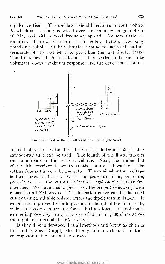
SEC. 63] TRANSMITTER AND RECEIVER AERIALS 333
dipoles vertical. The oscillator should have an output voltage E0 which is essentially constant over the frequency range of 40 to 50 Mc, and with a good frequency spread. No modulation is required. The FM receiver is set to the lowest station frequency noted on the dial.' A tube voltmeter is connected across the output terminals of the last i -f tube preceding the first limiter stage. The frequency of the oscillator is then varied until the tube voltmeter shows maximum response, and the deflection is noted.
Oscillator a
Dipole of muéh shorter length than dipole to be tested
05/
Actual feeder of length as used in the
051 installation
Actual receiver dipole r'
FM-Receiver
FIG. 105.- Testing the overall sensitivity from dipole to set.
Instead of a tube voltmeter, the vertical deflection plates of a cathode -ray tube can be used. The length of the linear trace is then a measure of the received voltage. Next, the tuning dial of the FM receiver is set to another station allocation. The setting does not have to be accurate. The received output voltage is then noted as before. With this procedure it is, therefore, possible to plot the output deflections against the carrier fre- quencies. We have then a picture of the over -all sensitivity with respect to all FM waves. The deflection curve can be flattened out by using a suitable resistor across the dipole terminals 1 -1'. It can also be improved by finding a suitable length of the dipole rods, which is a good compromise for all FM stations. In addition it can be improved by using a resistor of about a 1,000 ohms across the input terminals of the FM receiver.
It should be understood that all methods and formulas given in this and in Sec. 63 apply also to any antenna elements if their corresponding line constants are used.
www.americanradiohistory.com

334 FREQUENCY i!OU(ILAT!O.V [CHAP. V
64. Linear Conductors Used as Radiators. -As far as the radiation pattern of conductors excited in the 0.5X, X, 1.5X, etc., distributions are concerned, reference is made to Fig. 106. It is
seen that only the 0.5X distribution has a decided directivity since all other distributions have several radiation lobes. When a
Broad side
t
/ = /.5A Fta. 106. -Horizontal radiation pattern of horizontal dipoles of total length lin terms of
different wave -length distributions.
Broad side
concentric line is mounted perpendicular to ground and so dimen- sioned that it has a characteristic impedance Zo = 37 ohms, it can be used for feeding without any reflections a quarter -wave- length radiator as shown in Fig. 107. This condition then causes the indicated distributions. As long as the diameter of the inside conductor extension is a small fraction of the radiator length 1,
the radiation resistance at the input point 1 is essentially inde-
www.americanradiohistory.com
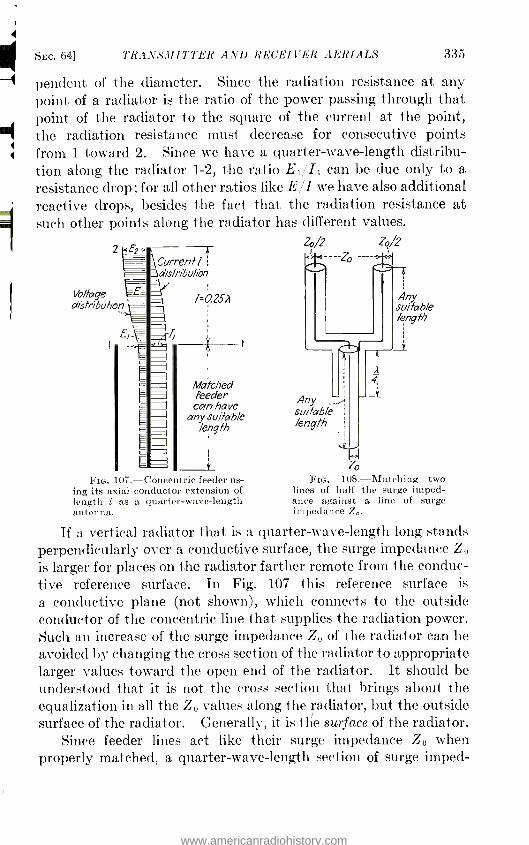
SEc. 641 7'RANS!IIITTER AND RECEIVER AERIALS 335
pendent of the diameter. Since the radiation resistance at any point of a radiator is the ratio of the power passing through that point of the radiator to the square of the current at the point, the radiation resistance must decrease for consecutive points
i from 1 toward 2. Since we have a quarter- wave -length distribu- tion along the radiator 1 -2, the ratio E1 /I1 can be due only to a resistance drop; for all other ratios like E/I we have also additional reactive drops, besides the fact that the radiation resistance at such other points along the radiator has different values.
2 E2 4/2 4/2
Current distributibn
Vo/tage distribuhon 1=0.25.i
Matched feeder can have
any suitable length
Flo. 107. -Concentric feeder us- ing its axial conductor extension of length l as a quarter- wave- length antenna.
Any _
suitable length
1 4 FIG. 108. -Matching two
lines of half the surge imped- ance against a line of surge impedance Zo.
Any suitable length
If a vertical radiator that is a quarter -wave -length long stands perpendicularly over a conductive surface, the surge impedance Zo
is larger for places on the radiator farther remote from the conduc- tive reference surface. In Fig. 107 this reference surface is
a conductive plane (not shown), which connects to the outside conductor of the concentric line that supplies the radiation power. Such an increase of the surge impedance Zo of the radiator can be avoided by changing the cross section of the radiator to appropriate larger values toward the open end of the radiator. It should be understood that it is not the cross section that brings about the equalization in all the Zo values along the radiator, but the outside surface of the radiator. Generally, it is the surface of the radiator.
Since feeder lines act like their surge impedance Z0 when properly matched, a quarter -wave- length section of surge imped-
www.americanradiohistory.com

336
ance Zo can be used ances Zá and Zö by
FREQUENCY MODULATION [CHAP. V
for matching two feeder characteristic imped- choosing
Zo = (198)
After all, lines act like their lumped equivalent values and we can, therefore, connect lines in series or in multiple and apply ordinary laws holding for lumped circuit constants. When two feeders act with their respective surge impedances Zo and Zö in series, the result is an impedance Zó + Z'o' ; for a parallel connection of the two feeders, we have the resultant impedance 4o4'/(4 + Zo). Figure 108 shows how this is done in actual designs. Figure 109
AI B
Can be any suitable length
Lines have surge impedance
Zo= 500 ohms--------
71 meters ="W
8 62 ' !; - !.
Zo 13 =k3A
D2
16-k6A
Zo
is l5 k-A Ca' an be any
suitable length
High frequency source which is frequency modulated
(a) (b) Fha. 109. -High- impedance lines as dipole feeders.
shows how relative phases as well as amplitudes of currents exciting the dipoles D1 and D2 can be obtained from a single common h -f source. This case has a direct application when dipoles, as in turnstiles, have to be fed in time phase quadrature. With respect to Fig. 109a, the constant k5 is 0.95 X 0.25, so that quarter -wave -length excitation takes place on this stub. The length ll can be any suitable length, as far as the phases are con- cerned. Nevertheless, the shortest feasible length should be used in order to keep the feeder losses to a minimum value. If the other length is ll + 0.95 X 0.25X, then the dipole D2 will be excited with a current that is lagging 90 deg behind the current that excites the dipole D1. The constant 0.95 holds very well in
---- lifeefl - - - I
\V c feet
Zo-- ,d feet
Zo =600 ohms
c =7Sd 1.4674 feet
a= FMcfeel
b =FM6 feet
www.americanradiohistory.com

SEC. 64] TRANSMITTER AND RECEIVER AERIALS 337
the FM range of carrier frequencies for normal conductor dimen- sions. It assumes that the group velocity c" of power transfer occurs 5 per cent slower than in empty space. Stubs of lengths l2 and l3 are used for bringing about the proper matching with the respective input impedances across terminals 1 -1' and 2 -2'. The sketch in Fig. 109b shows how a half -wave radiator rod is
excited with a parallel feed if a 600 -ohm parallel line feeder is
employed. The formulas given hold likewise for frequencies well in the FM range of carrier frequencies.
The Q value of a line is the ratio of its total effective reactance at the operating frequency to its total effective resistance. Hence, the smaller the Q value, the less the feeder will be affected by frequency deviations from the center frequency. In other words, the electromagnetic storage ability of the feeder should be com- paratively small if the feeder is to be used over quite a wide band of carrier frequencies as in FM systems. On page 328 we have shown how the Q value of a feeder can be computed from actual experimental data. It is a hyperbolic sine function for quarter - wave- length feeders, and depends only on the attenuation a of
the feeder. Hence, when impedance transformations are to be made between the terminating points on an aerial and the source of an FM transmitter, or the input terminals of an FM receiver in case of reception, several quarter- wave -length feeders should be cascaded rather than making the impedance transformation in one step with only one quarter- wave -length feeder. Such cas- cading causes a lower over -all Q value since the resultant reflection loss is actually smaller than the emphasized reflection loss for only one large step impedance transformation. The most ideal case would be an infinite number of quarter -wave impedance transformations.
This brings us then to an exponential surge impedance taper Zoe " where p = 360í/X deg. This can be done with a Lecher
wire system, which instead of using parallelism has a suitable spread along the length l of the feeder. Such an exponential wire system could lead only to a limited lower termination of
about 150 ohms (see Fig. 97, curve for parallel wires), from a practical point of view. Also from a practical point of view it would be difficult to keep such a mathematical spread in an actual outdoor installation. An exponential surge impedance variation along a feeder could also be obtained by having a
www.americanradiohistory.com

338 FREQUENCY MODULATION [CHAP. V
suitable expansion of the concentric outside cylinder of a con- centric line. According to the corresponding curve of Fig. 97, very low terminations can then be matched efficiently.
It must be stressed again that we are chiefly interested in low - impedance terminations in present -day FM systems since more power can be extracted from an arriving electromagnetic field. With present -day FM antenna arrays it is likewise more or less a low- impedance termination that is required. The low- impedance feeder has, in reception, the added advantage that it will keep out more interference, just as in feeders used in the 'audible range of frequencies, "hum" is kept out more with 50 -ohm lines than with 1,000 -ohm lines.
An ideal impedance transformation could also be obtained by using two flat strips which are equally spaced but which change their areas along the length direction in order to cause an exponen- tial decrease of Zo. With such an arrangement, we have at first a rather rugged structure as well as a means for obtaining very large impedance transformations, which can be made to yield on one side very low Zo values. The exponential taper of the surge impedance could also be affected by keeping the area of both flat conductors for the go and the return the same but causing a suitable spread toward the length direction. The practical design would then be more difficult. Besides the wind pressure would be more severe, since larger areas are used as well as "wind pockets" provided.
65. Excitation of Dipoles.- Suppose we have two dipoles in one plane as shown in Fig. 110. The respective feeder gaps 1 -1' and 2 -2' of the dipoles A -A' and B -B' are taken just large enough to allow the supply of power that excites the respective dipoles and to prevent mutual contact. We can cause half -wave excitations 1.1 and I2, which have generally unequal amplitudes at terminals 1 -1' and terminals 2 -2' as well as unequal phases 'Pi and i'2. The relative time phase is then generally ' = - 42. The electric fields sl and 82 due to the respective dipoles are proportional to the dipole current distributions. If the two dipoles make any given space angle O with each other, instead of 90 space degrees as indicated in Fig. 110, we have
81 = k11 sin (S2t) sin 82 = kI2 sin (S2t - 9) in 1,1.25
(199)
www.americanradiohistory.com
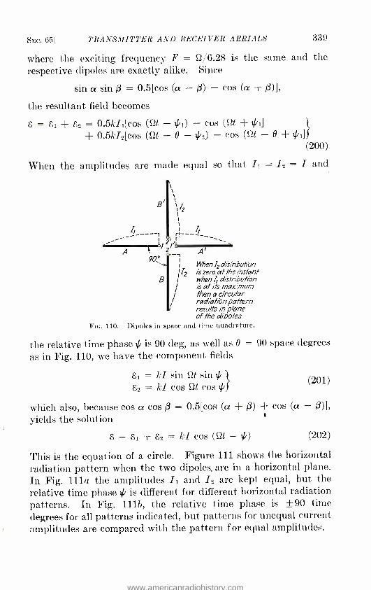
SEC. 65] TRANSMITTER AND RECEIVER AERIALS 339
where the exciting frequency F = 12/6.28 is the same and the respective dipoles are exactly alike. Since
sin a sin ß = 0.5[cos (a - ß) - cos (a + ß)],
the resultant field becomes
8 = 81 + g2 = 0.5k11[cos (S2t - lÿl) - cos (S2t + 4'1]
+ 0.5k12[cos (S2t - B - 42) - cos (Slt - O + 4',] (200)
When the amplitudes are made equal so that I1 = I2 = I and
A 90°
I
2 A' When I2 distribution is zero at the instant when 1 álstribution is at its maximum then a circular radiation pattern results in plane of the dipoles
i ¡I2
FIG. 110. -Dipoles in space and time quadrature.
the relative time phase 4' is 90 deg, as well as B = 90 space degrees as in Fig. 110, we have the component fields
81 = kI sin Slt sin i/i
82 = kI cos Slt cos 4' j
which also, because cos a cos ß = 0.5[cos (a + ß) + cos (a - ß)],
yields the solution
8 = 81 + 82 = kI cos (S2t - 4')
(201)
(202)
This is the equation of a circle. Figure 111 shows the horizontal radiation pattern when the two dipoles. are in a horizontal plane. In Fig. 111a the amplitudes I1 and I2 are kept equal, but the relative time phase 4' is different for different horizontal radiation patterns. In Fig. 1116, the relative time phase is +90 time degrees for all patterns indicated, but patterns for unequal current amplitudes are compared with the pattern for equal amplitudes.
www.americanradiohistory.com

340 FREQUENCY MODULATION [CHAP. V
66. Transmitter Antennas. -In order to cover a large service area, a horizontal circular radiation pattern is required. A vertical half -wave dipole will give such a pattern. In FM trans- mission it is also necessary to have such an FM power transfer from the last power stage toward the antenna array as to avoid as much as possible phase distortion and amplitude modulation.
(eta
' -_ Constant phase ' k =óS difference 11)=90°
but varying currents '-k =I
(b) FIG. 111.- Radiation patterns in crossed dipole plane.
lI =12 but varying phase 4
(a)
12 No.2
No.2
The former would cause equivalent parasitic frequency modulation. Such effects can be kept down if the antenna array has a sufficiently broad input impedance with respect to the maximum peak -to- peak frequency swing.
In order to obtain a large horizontal field gain, it is also neces- sary that the transmitter aerial array concentrate the high -angle radiation toward the horizontal service plane. Half -wave dipoles, as indicated in Figs. 112a and 113, satisfy such conditions. The vertical dipole array, also known as the Franklin antenna, has inherently a circular horizontal radiation pattern like all single half -wave radiators in planes perpendicular to the conductor axis.
www.americanradiohistory.com
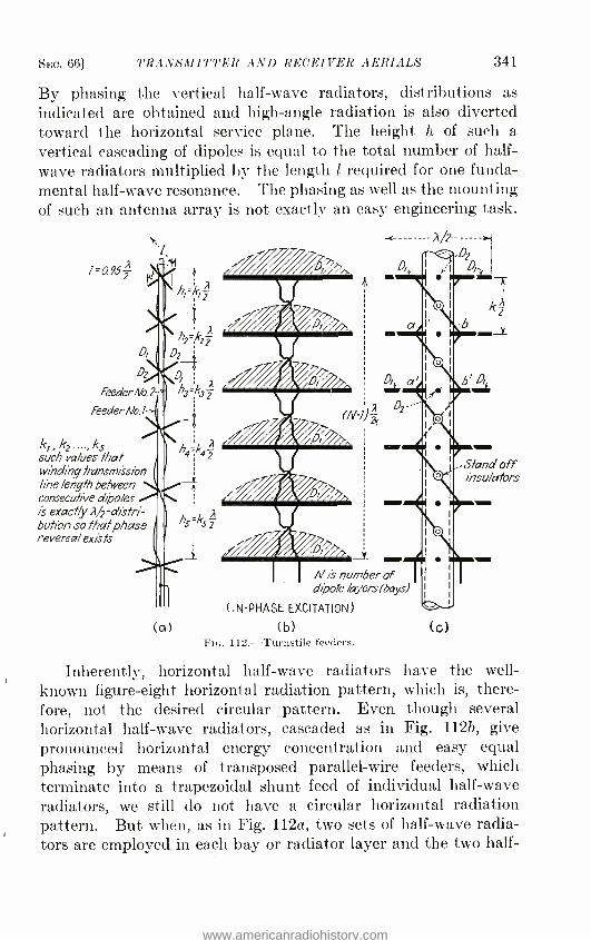
SEC. 66] TRANSMITTER AND RECEIVER AERIALS 341
By phasing the vertical half -wave radiators, distributions as indicated are obtained and high -angle radiation is also diverted toward the horizontal service plane. The height h of such a vertical cascading of dipoles is equal to the total number of half - wave radiators multiplied by the length l required for one funda- mental half -wave resonance. The phasing as well as the mounting of such an antenna array is not exactly an easy engineering task.
1=0.952 I`1
-T h,=k,i
--4 hz ;kz2
D,
Oz D2 D,
FeederNo.2 ha°k3 i Feeder No.1-
k, , k2 ...., ks such values that winding transmission line length between I consecutive dipoles is exact/y 2/2 - destri= bubon so that phase reversa / exists
2
hs=ksz
(a)
. L D,Y
At
T
T °.:r
(N-1)-- a D2
---
T J%%.,f_
T
1
-Stand off insulators
N is number of dipole layers (bays)
(IN-PHASE EXCITATION)
(b) Fie. 112.- Turnstile feeders.
(c)
Inherently, horizontal half -wave radiators have the well - known figure -eight horizontal radiation pattern, which is, there- fore, not the desired circular pattern. Even though several horizontal half -wave radiators, cascaded as in Fig. 112b, give pronounced horizontal energy concentration and easy equal phasing by means of transposed parallel -wire feeders, which terminate into a trapezoidal shunt feed of individual half -wave radiators, we still do not have a circular horizontal radiation pattern. But when, as in Fig. 112a, two sets of half -wave radia- tors are employed in each bay or radiator layer and the two half-
www.americanradiohistory.com

342 FREQUENCY MODULATION [CHAP. V
wave radiators in the same horizontal layer or bay cross under 90 space degrees, we can obtain a circular pattern. To accom- plish this, all D1 dipoles are excited in time quadrature with respect to all D2 dipoles. Figure 113 shows that this pattern is a maxi- mum in the horizontal plane while the vertically polarized com- ponent vanishes in this plane.
From Fig. 112a we also note that there is no difficulty at all in feeding a turnstile antenna as originally suggested and developed
At instant of maximum D excitation Vertical
Ill iL k í-' N r
o AEI ,0
AIM il (A1} =h N=h k;n iß ' -'
d, /;qs i
7.0 0 g s6.0
.E á 5.0
á 4.0
3.0 Ç á, 6 2.0
I.0
á > 0 o
fra
LO 2.0 3.0 4.0 hin wave length -..
Norizontallypolarized electric vector
Vertically polarized vector
1.0
0.8
0.6
0.4
0.2
0
0.2
90 80 70 60 50 40 30 20 10 0 -04
-Zenith angle 6 FIG. 113. -Comparison of horizontal dipole bays with vertical half -wave radiators.
by G. H. Brown. A common source, which is the output of the last power stage of an FM transmitter, then supplies the output power to a feeder system, as is described in connection with Fig. 109. The two lengths 11 and ll + 0.95X/4 bring about time quadrature, i.e., a phase difference of 90 deg. The connections A- B and A' -B' of Fig. 109 then are the connection points on the lowest dipole D1 and the lowest dipole D2 of Fig. 112a. All other dipoles are then connected by the respective dipole interfeeders 1 and 2, where feeder 1 feeds all D1 half -wave radiators and feeder 2 supplies power to all D2 half -wave radiators.
Figure 112e shows how simply this can be done. The D, dipoles are then in the plane of the paper and the D2 dipoles are
TURNSTILE FRANKLIN N= Number of bays
Note. Vertical vector polarization is zero in horizonta /plane
www.americanradiohistory.com
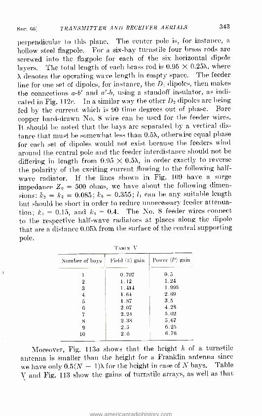
SEC. 66] TRANSMITTER AND RECEIVER AERIALS 343
perpendicular to this plane. The center pole is, for instance, a
hollow steel flagpole. For a six -bay turnstile four brass rods are screwed into the flagpole for each of the six horizontal dipole layers. The total length of each brass rod is 0.95 X 0.25X, where X denotes the operating wave length in empty space. The feeder line for one set of dipoles, for instance, the DI dipoles, then makes the connections a -b' and a' -b, using a standoff insulator, as indi-
cated in Fig. 112c. In a similar way the other D2 dipoles are being fed by the current which is 90 time degrees out of phase. Bare copper hard -drawn No. 8 wire can be used for the feeder wires.
It should be noted that the bays are separated by a vertical dis-
tance that must be somewhat less than 0.5X, otherwise equal phase for each set of dipoles would not exist because the feeders wind around the central pole and the feeder interdistance should not be
differing in length from 0.95 X 0.5X, in order exactly to reverse the polarity of the exciting current flowing to the following half -
wave radiator. If the lines shown in Fig. 109 have a surge
impedance Zo = 500 ohms, we have about the following dimen-
sions: k2 = k3 = 0.085; k6 = 0.355; ll can be any suitable length but should be short in order to reduce unnecessary feeder attenua- tion; k5 = 0.15, and k4 = 0.4. The No. 8 feeder wires connect to the respective half -wave radiators at places along the dipole
that are a distance 0.05X from the surface of the central supporting pole.
TABLE V
Number of bays Field (g) gain Power (P) gain
1 0.707 0.5 2 1.12 1.24 3 1.414 1.995 4 1.64 2.69 5 1.87 3.5 6 2.07 4.28 7 2.24 5.02 8 2.38 5.67 9 2.5 6.25
10 2.6 6.76
Moreover, Fig. 113a shows that the height h of a turnstile antenna is smaller than the height for a Franklin antenna since
we have only 0.5(N - 1)X for the height in case of N bays. Table V and Fig. 113 show the gains of turnstile arrays, as well as that
www.americanradiohistory.com
344 FREQUENCY MODULATION [CHAP. V
of a Franklin antenna, over the value that would be obtained in case of a single half -wave radiator. Hence, for a six -bay turnstile, a 2.5 -kw transmitter would act as though a 2.5 X 4.28 = 10.7 kw supply were used in comparison to a single dipole transmitter antenna.
The turnstile of the General Electric Company contains only three bays spaced vertically about 270 electrical degrees apart instead of 180 deg. The radiation elements are also shunt -excited from a concentric line by a conductor connected through a series capacitor a short distance from the pole. Also here the correct phase relation and current distribution between the various antenna elements is obtained by an appropriate phasing section of the feeder located below the radiating system of the half -wave radiator array. An impedance- matching section is used to provide the correct termination for a 150 -ohm balanced feeder. The theoretical field intensity s caused by such an array in the horizontal plane has then an average value of 3.7 db above the radiation from a single half -wave radiator in the direction of maximum radiation. This is 7.3 db above a single -section turn- stile. The theoretical gain of the General Electric turnstile is about 0.4 db above the four -section turnstile with 180 electrical degrees vertical separation between consecutive bays. In this system we have also a balanced 150 -ohm feeder branching into two single conductor transmission lines of 75 ohms each.
That turnstiles are rugged self -supporting structures can be seen from the fact that in some installations the overturning moment at the base of the tower is in the neighborhood of 48,600 ft -lb. It is also noteworthy that the lighting connection to the top of the turnstile is completely shielded since the wiring is mounted within the supporting center pole. It is also possible to mount the turnstile on top of an ordinary broadcast tower as long as this tower can withstand the overturning moment due to abnormal wind pressure and due to the increased height.
67. Quarter -wave -length Feeder Sections. -We have learned on pages 311, 335 that such sections are being used for matching unequal impedances Z1 and Z2 by means of the surge impedance Zo = -VZ1Z2 of the matching section. The "teeter- totter" action given by this square -root relation can exist only when the feeder is exactly 90 electrical degrees long. If the group velocity c" of wave propagation along the feeders is the same as the
www.americanradiohistory.com

SEC. 67] TRANSMITTER AND RECEIVER AERIALS 345
velocity c of light, the physical length l of the matching section would be equal to one -quarter of the operating wave length X.
We have then generally the formula
l = 4 = 246 F (203)
where the length l of an impedance- matching feeder is in feet, the operating frequency F in megacycles per second, and k denotes a factor that expresses the ratio c " /c, i.e., the fraction of the group velocity to the velocity of light. From the discussion given at several places in this text, it is evident that the value of k is
closest to unity value when the feeder section is as "open a trans- mission line" as possible. For this reason customary Lecher wires show a k value in the neighborhood of about 0.96 to 0.98. A
concentric line with air as a dielectric shows values of k from 0.87 -0.95, where the upper limit holds generally for good lines of this type. Concentric cables with rubber insulation slow down the energy propagation considerably on account of the large dielectric loss and k = 0.5 - 0.6. About the same k values hold also for twisted leadins. The accurate values of k can be easily found by experiment.
www.americanradiohistory.com


APPENDIX This supplementary part gives solutions and tables that were actually used in the
discussion of the preceding chapters. The tables are written in such a form that the spectrum distribution of the modulation energy can be directly noted by mere inspec-
tion. The arguments are given in terms of radians since this gives actually the numerical value of the ratio sF /f in case of true FM and the value of AO in case of
true PM. In case of indirect FM, the arguments stand for k M/f where k takes care
of the modulation efficiency. The tables with the argument ß can also be used for
finding the decay factors c that may be needed in the evaluation of the speed of
electrical actions if several circuits transfer desired as well as undesired information. There are also tables on the Si, Ci, and the corresponding integral epsilon functions. They apply to cases where the self- as well as the mutual impedance of radiators and feeders is concerned. Since, by means of such tables in connection with formulas given in the text, it is possible to compute the reactive or the resistive component of a
conductor, we can, with the numerical result, also find the Q value of a conductor. At this point it should be again realized that in many systems a high Q value is not at all what is desirable. For instance, when a quarter- wave -length section of a line,
as a concentric tank, is used for an interstage coupling in short -wave work, a high
impedance is desired; for a concentric tank used as the frequency -determining branch,
it is a high Q value that is of interest. It should also be realized that neither a Lecher
wire feeder nor a concentric line feeder, even when acting aperiodic, can be considered
as being absolutely free from radiation effect, even though the radiation resistance of a
concentric line is relatively smallest. Generally, the radiation resistance of a feeder
depends on the exciter frequency, on the length of the line in terms of wave length, as well as on the termination. Even though there is the general understanding that a shielded feeder like a concentric line, when terminated into its surge impedance Zo,
does not radiate, it should be noted that it has a radiation resistance just the same.
As a matter of fact the radiation resistance is equal to the sum of the radiation resistance of the open -ended feeder of the same length as the aperiodic feeder and the radiation resistance with the far end short -circuited. Even though the magnitude of the radiation resistance is small, it can greatly affect the Q value in the upper megacycle range as, for instance, used in FM relay work.
68. Theory of the Spectrum Solution. -There are two places in the literature which date back to the years 1887 and 1862 that have to do with the definition of
"instantaneous frequency," which applies to present -day FM even though applied in those years to acoustical problems. Lord Rayleigh in 1887 treated the case where
the tension of a string is periodically varied. This is the mechanical case correspond- ing to the capacitance variation in an oscillatory system. Helmholtz in 1862 solved the difficulty by defining the instantaneous frequency in an acoustic system as
S2, = dF, dt
It is the corresponding integral solution that we employ today in order to include also
the integration constant. It is attributable to J. R. Carson who published in 1922, for
the first time, a solution for the spectrum distribution when a high -frequency current is modulated in frequency due to a sinusoidal variation in the circuit capacitance.
347
www.americanradiohistory.com
348 FREQUENCY MODULATION
In 1930, B. van der Pol followed up the contribution of Carson and gave the concept of the modulation index. He also treated the case when a variation of the circuit capacitance is instrumental in causing FM and solved the obtained differential equation by a method leading to the result found by Carson. He gave also a solution for the case of code modulation, i.e., when the value of the circuit capacitance C, jumps periodically and discontinuously from a value of C - AC to a value of C + AC, and vice versa. W. L. Barrow in 1933 discussed the case of direct capacitance modulation, direct frequency variation, and inverse capacitance modulation. The list of references should be consulted for any other details, since the following dis- cussion applies only to the case, as frequency modulation is used to -day, for which the signal frequency f is small compared to the carrier deviation frequency AF; the maximum frequency deviation of is also small compared with the center fre- quency F. The derivaton for the energy distribution in the frequency spectrum is then as follows.
Suppose that we have the case of a reactance modulation where the tank capaci- tance value is C in absence of modulation, and is affected by an injected parallel capacitance variation of maximum swing AC when modulation is present. We have, therefore, to deal with an instantaneous circuit capacitance C, and a fixed circuit inductance L. Hence, we have no longer an oscillation constant CL but an oscillation factor C,L, which varies during the modulation cycle of 1/f sec. The well -known differential equation then reads
Ld+e=0 if L denotes the tank inductance, i the instantaneous tank current with an instan- taneous condenser voltage e. The effect of the circuit resistance R is ignored since we think in terms of a tube oscillator where the negative resistance action neutralizes the R effect. Besides, the small change of the term R /(2L) is fixed and has nothing to do with the frequency changes due to the modulating current. Since the cor- responding charge is dq = i dt and e = q /C,, we obtain
dtg + C,L - 0 (204)
Since
SZe = 6.28Fe - 1 (205)
we can also write
dtq + q14 = 0 (206)
-VC7L
Hence Eq. (205) holds for FM while S2 = 6.28 F = 1/ VOL holds in absence of modulation.
It does not seem possible to solve Eq. (204) generally, as far as practical results are concerned. A solution is, however, feasible when we define C, or 52,. The definition for C, relates to the case of capacitance variation and the definition of S2, = 6.28 F, is the most direct case of frequency modulation. Such definitions actu- ally express what happens in case of present -day direct FM. Suppose a reactance tube injects the variation C; = AC cos wt, then
C, = C + AC cos wt (207)
is the required definition. Assuming that OC < C, which is always the case in direct FM, we find, by binominal expansion of the instantaneous circuit capacitance C,, for
www.americanradiohistory.com

APPENDIX 349
the reciprocal of the oscillation factor
1 = - S24(L 4C) cos wt + 126(L 4C)2 cost wt - + (208) CIL
Equation (204) then becomes
-dtq q(Ao + Al cos wt + A2 cos 2wt + ) = 0 (209)
In this expressions Au, Al, A 2, etc., are constants obtained after completing the opera-
tions contained in Eq. (208) and grouping the terms according to increasing signal
frequency angular velocities wt, 2wt, etc. Assuming 4C « C, Eq. (208) simplifies
and the terms with (4C)2 and still higher powers of 4C may be neglected. We have,
therefore, 1 ^- 522[1 - 02(L 4C) cos wt] = 522 (1 - cos cat)
C,L
522 (1 + 2 of
cos wt'
C L '- S22
(1 + 2 FF
cos wt) (210)
Here 4F denotes the absolute frequency change, which is the difference between
the assigned carrier or center frequency F and F -/1 - 4C /C. The limitation of
AC « C brings us then to the differential equation
dtq q(02 + 212 452 cos wt) = 0 (211)
This simplified expression of Eq. (209) is the basic relation used by Carson as well
as by van der Pol in obtaining the spectrum solution. The limitation of differential
equation (211) is, therefore, that the maximum frequency deviation 4F must be very small compared with the value of the center frequency F. Hence, the spectrum solution (12) is based on such an assumption. This should not be overlooked if,
some day, we expect to apply OF swings which are not very small with respect to the
center frequency F. If we use the differential equation in the form as expressed by Eq. (206), we have
a means for finding out what condition prevails when the frequency F, = 52,/6.28 is
directly varied instead of the capacitance of the tank. This is actually the case of
true frequency modulation as would happen in an alternator whose speed experiences
oscillations, i.e., vibrates about its mean speed. We have then F, = F + 4F cos wt
and, when multiplied on each side by 6.28, the case for the corresponding angular
velocity at any instant of time. Equation (206) then yields the differential equation
dtq q(S22 + 0.5 4122 + 252 412 cos wt + 0.5 ASP cos 2wt) = 0 (212)
This expression has no limitation and holds for all values of 4F and F. But when 4F «F, we obtain also here the expression given in Eq. (211). With this limitation we are, therefore, confronted with the solution of the differential equation
dtq + 522 (1 + 2 F cos cat) t 1 q = 0 (213)
This expression, which defines a Mathieu function, is well known in theoretical physics. Hence, if we make the substitution
q = E fxdt
www.americanradiohistory.com

350 FREQUENCY MODULATION
we find ds dt + x2 + 122 ( 1+ 2T, cos wt) = 0 (214)
This brings us to a first -order equatión of the Iticcati type. If we also make the additional assumption that 4,F /f is small, as is the case in present -day FM, besides the assumption that f «F, we have the approximate solution
x1.2 = ±j12 \11 + 2 -FAF cos wt ^- ±j(12 + A0 cos wt) (215)
The solution of (213) with such assumptions as are justified is then
q = efyls` + 6J std` = k cos If (12 + Al2 cos wtt )dt] / \ = k cos 1 Stt + - sin cot) = k cos 1 1lt + sin wt 1 (216) w
We note, therefore, that for f «F and of «F, the cosinoidal modulation function in the C, variation causes a corresponding sinusoidal frequency variation. This can be explained by the Helmholtz definition for the instantaneous value of 12, which yields
0S2 .
dF, d ( Al2 \ dt dt
e cu
sin cot) = 12 + OS2 cos wt
The square of this result yields the approximation
122 (1 + 2 F cos wt)
which checks the second term of Eq. (213). In the solution of Eq. (216) the arbitrary phase constant has been ignored since
it would not contribute anything to the discussion presented here. Putting the amplitude value k of Eq. (216) equal to unity, we can expand this equation and find for ß = of /f
q = cos (12t + ß sin wt) = cos SU cos (ß sin wt) - sin W sin (ß sin wt) = cos y cos z - sin y sin z (217)
where z = ß sin wt and y = W. For wt = p, according to Fourier
cos (ß sin p) = Jo(0) + 2J2(6) cos (2p) + 2J4((3) cos (4p) + 2J6(ß) cos (6p) + -
sin (ß sin p) = 2J1(ß) + 2J2(0) sin (3p) + 2J60) sin (5p) + 2J7(0) sin (7p) + -
(218) But
cos y cos z - sin y sin z
Hence, Eq. (217) yields
q = cos (12t + ß sin wt)
= cos (y + z)
= Jo(ß) cos 12t - JI(ß)Ecos (12 - w)t - cos (12 + w)t]
+ J2(13)Ecos (12 - 2w)t + cos (12 + 2w)t] - J2(ß)[cos (12 - 3w)t - cos (12 + 3w)t] + J4(13)[cos (0 - 4u)t + cos (12 + 4cu)t]
(219)
(220)
which is exactly the spectrum solution used in Eq. (12) except that Eq. (12) is ex- pressed in sinus terms, which should not matter as far as the frequencies are con- cerned. We have, therefore, the Bessel coefficients J0(3), J1(ß), J2(ß), J3(0), J4(ß),
www.americanradiohistory.com

APPENDIX 351
etc., of the first type, where for the above derivation the modulation index ß stands for AF If and we have the respective spectrum frequencies F for the center frequency; F ± f for the first side -current pair; F ± 2f for the second side -current pair; and F ± of for the nth side -current pair.
Table VI gives an extension of the Bessel tables given in the text up to a modula- tion index ß = 24.
The Bessel function of the first kind .1 Jn(ß) is, when n = 0 or a positive integer, given by the convergent series
n Jn(ß) = 2n n!)
1
02 04
2(2n + 2) + 2 4(2n + 2)(2n + 4)
/36
+ J 2.4.6(2n +2)( 2n+4 )(2n + 6) (221)
since it satisfies the Bessel' differential equation
d2Jn(ß) 1 dJ (ß) 2l ß dß + 1 - ! Jn(0) = 0
The series for J,(ß) becomes essentially useless in case of numerical computations when the modulation factor ß is even moderately large. For this reason this function is expressed in another series form which is well adapted for numerical computations for large ß values,
l l J(ß) = V 10 [an cos (ß - 2n 4+ 1 b sin \ß
- 2n 4 1 / J
(222)
for
(4n2 - 1) (4n2 - 9) (4n2 - 1) (4n2 - 9) (4n2 - 25) (4n2 - 49) an = 1 -
2!(80)2 + 4!(85)4
b,, 4n2 - 1 (4n2 - 1)(4n2 - 9)(4n2 - 25)
80 3!(8ß)2
For very large values of ß, the functions approximate the values given by
Jn(ß) \ 2n + 1
/ = # cos ß - a
(223)
(224)
' Generally Bessel functions of the first kind J (ß) and 1n(0) are given by the expression of Jn(5) as given in Eq. (221) and
In(ß) - 2 n) [1 + 2(2n + 2) + 2 4(2n + 2)(2n + 4)
/76 + 2 4 6(2n + 2) (2n + 4) (2n + 6) +
This function then satisfies /
d2óß2ß) + ß
dIdnß) (1 + Q2/
In(5) = O
The following interrelation then holds
I,(ß) = .i- nJn(ß) I _n(ß) = -n(0)
www.americanradiohistory.com

352 FREQUENCY MODULATION
Wr:4
Z H1
Z O - 3 J H +,,i,
á eq I
ó I
C
W + x F + ,., 54 C u
.1M 41 Cq + ,:: .
ha + G >
"i d
F m M. :q
Ñ F Q 3
ti+ 1 1
PI + V yv
Ç
C .a M a 3 . a 1 .. F ä
.z
W `/ v Z I .4
7 ° V w o 4 I + 1.
a I V c, 3M . C
+ + + a ? a a a w . O
Z ;} ú ú ÑT
m ,Ti. . 3 SI
0 ,--7; 1" '--z
W
m ++++ .7 z 'Pa
á F 5 i W
....A
6 II
IA:, U z
I
14
Ga
ti
co.
oumm M
mimti ¡.BaMOi-rylM IMÓOD.i ÓII r ÓÑO..tiOÑOMN0NOM0SSS
17,
..-, 0 0 0 0 0 0 0 0 0 0 0 0 0 0 0 0 0 0 0 0 II III ti ti
II
OZ
Op co - NWtiOM n OC ONÓ000 r -i ryo000OOOC-jMS i NONMOON0N0N0M0000 ,-, O O O O O O O O O O O O O O O O O O O II III
e II
O1
8 O 00C+0 OÁO.O.+M0W ` -r .r ti N
ti .OM3 000M.yÓc008 g O N .O N N O N M N NÑ O O 808 o
"s O O O O O O O O O O O O O O O O O O
0) II
OS
y.OtOM MM000+.f0ÓM.O-OtiÑMOOSÑM 0 O.Oy .O.Oyp. I.OVlNtOM-iO OÑNÓNMMN.N+ÓÓ08ÓÓ
ti 00000 i 00000000000
lrOÑñ.O+ONi m M
II
iy.MtiONNOÓÓ II , yÑ.wÑMMÑ.iO000B
0000000000000000 a III Ó N \ pNIMM.O[J t-
111+ 100000
d V W
O Ñ O ñN VbÑMOOtiSO II NNrMMNNONO S 7 000000000000
I I` OO.rNCMO ... ÿ ti24.,M II
NdtOO.cOM.r>.. o MOMMN.+0080 Z1. , 0 0 0 0 0 0 0 0 0 0 0 II e " ÿ IBeMÓ~-NOOi.O?
Il vO<O[OMOJenW.-O MOMd.N000
O17 000000000 I I
o, 0..r, TiÑOM M M OMOOMCe+X-MÑ
II G NMd.M..000 OD ti 00000000
N N Ñ O.Io00.+ Ó Ñ
II _. M.OnNOONwnO ,.. N.eOM.+O O
0 0 0 0 0 0 0 ^ NyO.. OO
II
vOdQN ñ :S ó 'CL, Oó000
E
g átiÑM M
`i, -I-I+1+i+1 +I s. iLi.R. C
y'° ° ,.s,,,,,,,,_...,.....,.. ....... c O.tiNM.a..O.O,000.Oti.Ni.Mi.i.-.OiÑW.O+ÑNÑÑÑÑÑNÑÑMMMMM
www.americanradiohistory.com

4
APPENDIX 353
Ñ
Q1 .-,
eDMyfDGVSÓ M O.
CO O M 0 M .'.n 07 O O..n+ S O NOMMOM.tOaa.MO.mOtOM....aO.aM.. OnwS N OC M. MN a00 O,m N00 mDy. M.OaM ,ON..ON. 0.0a00tOOMaMDOnn ÓOOpÓMÑÓÓSSSO O.O.Oy 0..O..0....OÑV-OO ÓII
0 0 0 0 0 0 0 0 0 0 0 0 0 0 0 00000000000000000000 1111
Ñ II
CO.
M ..
,
.00.. tmav`0
N N. CO Ñ OO 00 N l O. N a.,0 t 00 .O0 a0 l.nO..M.MMON<OOO>..00O..00IN.+t`MaOIV..00MVOd.. NO.O.N...00M ,NNM,,000.u'J.00OOOOCO,,I`O...WN.+O cOM.pOV.tiO.<OO.OMVIM.y.0000M..]NMO.JOtOMN.+000 O. O.-..- O.+ 0.+.- 0.+.- O'..+. O.+ N N N.- . 0 0 0 O O O O S Ì0000000000000000000000000000000000
II ,O. "-,
.GM<O m uO0
ó: Óti.M.MtMOtMOMONOtitiTeO0O,0OOMVO.00+ÑÓ0Oi W ti00+O.00ÑÓÓ~pp .N......M-iÓ.M+Ór.Ór.S.O+S..+.+^ÓÑÑNÓÓÓOSSSSO 00000000000000000000000000000000 Ì
Ñ II
Q7.
.^ N
..>
mc.. ,,me.,-,,mm .mO..cOiOltcONlñ NOM.00O..Ó.00.ON..,.O .NOO...iO.M.. 0.0.[.0MI`N.O.+OOMN.00NNO.W.NO.,0000.N000 M.NnN.000[Mal`MmOM...Oma...D00MN.-.00000 0.0.0.'+^.0r..0.N.+OtiNNN..-r000000000
III III III Ñ
II
,O.
Ó c
'',
o a..tia
óóoó.N..°OVN.m.ñcOO.M.áá+óo.Nnm.~.oóó00áw.W.óóó O ÓNÓOaSaÑÑÓSSSSS .o.O..O.. ..c....N..00S 000000000000 Ì ii 0000000000000000
0 II
m. ,
0 ñ a .00rr l <DOO.MM.MO"O [OLoOV.ppD.OMOOM.N..O/oÓ.00MñÁñOM.mpÓ yOiÑ00Ó[..O.Ó.Ga.00O.O..MM.ON.O.-i.Om..O 0
O..O....0..00N..O..c1NN....000Q-00 O0oS óóóóóóóóóóóóóóóóóóóóóóóóóóóóó
II
Ca ,
na a.cwoo MOpp.MfJMC...dOWO.m1.NÓ<O.O¡..O.OImOOOtiOO..oÑo 0000O00M.u.OJO.ÑmÓtiMm[O.]<OÑ.-.ÓMMÓ088 oO..O..0....N..0.c1clN...+000500 0000000000000000000000000000 III I IIII
I
(12.
pp 7y ti
MÓ88 pp pMO00ÑÑnÓSppS Ó..ÓN ..ÓÓSSO i' f'óólóóóóóó I I'óóóóóóóóóóóóóó
,o
II
Oa ..,
,00 O t N N V'MñbÓONO aaN.nan.nO.nNNawaawOamOOmrm.n.. ñ°o`DOó"póoó.N.`V °'ñmM."."póóSS ..Ó..ONO....O.NO..NÑÑ....00000000 00000000000 i 0 0 0 0 0 0 0 0 0 0 0 0 0 0
.Oy
II
CO.
O.
C
'
Oa00.N Ñ..ul.]ON..')..a00ÓQr[-VMN.MO.Ó.00O0Ó.0.V.O. a.O..aO.O.0aa000.<OOO.O...O.Da.Otp`M^.O OaO... OMlNO.$CVÑÑ..ÓÓ005SOO ONO.....m-iNO..NGO 0000000000000000000000000
I II III ti
II
T1.
. k
....
a M.'..~n ..aO<OOÑ~.000M.ÓO,..tOOO..[OJaMNtiótiÓM.N. ~MN..OÑm.00CN..a.00M00.000,WM.O.Op 0088 OONO..GV..ONNN....00OOS050 000000000000000000000000
II II L
II
01 ....
,
0o 00pp
O.N-O"0 oÓtiMOm...O.00ÓM..O00.00,.NÑCÓ Ñti..O..m..aaOMOOO..OM.. ONON....N..ONNN-...000SSSS 0000000000000000000000
II I
d e E
@
0 v
i
^ OÑ . M. M +I+I+I tl H d
21 s__w_.ö g
O..NMa.ncL000.0OO..NMa.geOr000.Or.NMa N N N N N N N N N N M M
www.americanradiohistory.com

354 FREQUENCY MODULATION
TABLE VII
x Si(x) Ci(x) Ei(x) Ei( -x) x Si(x) Ci(x) Ei(x) Ei(-x)
0.00 0 -. -=0 - m 1.7 1.4496 0.4670 3.9210 -0.07465 0.01 0.00999 -4.02798 -4.0179 -4.0379 1.8 1.5058 0.4568 4.2499 -0.06471 0.02 0.019999 -3.3349 -3.3147 -3.3547 1.9 1.5578 0.4419 4.5937 -0.05620 0.03 0.02999 -2.9296 -2.8991 -2.9591 2.0 1.6054 0.4230 4.9542 -0.04890 0.04 0.03999 -2.6421 -2.6013 -2.6813 2.1 1.6487 0.4005 5.3332 -0.04261 0.05 0.04999 -2.4191 -2.3679 -2.4679 2.2 1.6876 0.3751 5.7326 -0.03719 0.06 0.05999 -2.2371 -2.1753 -2.2953 2.3 1.7222 0.3472 6.1544 -0.0325 0.07 0.06998 -2.0833 -2.0108 -2.1508 2.4 1.7525 0.3173 6.6007 -0.02844 0.08 0.07997 -1.9501 -1.8669 -2.0269 2.5 1.7785 0.2859 7.0738 -0.02491 0.09 0.08996 -1.8327 -1.7387 -1.9187 2.6 1.8004 0.2533 7.5761 -0.02185 0.1 0.0994 -1.7279 -1.6228 -1.8229 2.7 1.8182 0.2201 8.1103 -0.01918 0.15 0.1498 -1.3255 -1.1641 -1.4645 2.8 1.8321 0.1865 8.6793 -0.01686 0.2 0.2000 -1.0422 -0.8218 -1.2227 2.9 1.8422 0.1529 9.2860 -0.01482 0.25 0.2491 -0.8247 -0.5425 -1.0443 3.0 1.8487 0.1196 9.9338 -0.01304 0.3 0.2985 -0.6492 -0.3027 -0.9057 3.1 1.8517 0.08699 10.6263 -0.0149 0.35 0.3476 -0.5031 -0.08943 -0.7942 3.2 1.8514 0.05526 11.3673 -0.01013 0.4 0.3965 -0.3788 0.1048 -0.7024 3.3 1.8481 0.02468 12.161 -0.00894 0.45 0.4450 -0.2715 0.2849 -0.6253 3.4 1.8419 0.00452 13.0121 -0.00789 0.5 0.4931 -0.1778 0.4542 -0.5598 3.5 1.8331 0.03213 13.9254 -0.00697 0.55 0.5408 -0.0953 0.6153 -0.5034 3.6 1.8219 -0.05797 14.9063 -0.00616 0.6 0.5881 -0.02227 0.7699 -0.4544 3.7 1.8086 -0.0819 15.9606 -0.00545 0.65 0.6349 0.04265 0.9194 -0.4115 3.8 1.7934 -0.1038 17.0948 -0.00482 0.7 0.6812 0.1005 1.0649 -0.3738 3.9 1.7765 -0.1235 18.3157 -0.004267 0.75 0.7270 0.1522 1.2073 -0.3403 4.0 1.7582 -0.1410 19.6309 -0.003779 0.8 0.7721 0.1983 1.3474 -0.3106 4.1 1.7387 -0.1562 21.0485 -0.00335 0.85 0.8166 0.2394 1.4857 -0.2840 4.2 1.7184 -0.1690 22.5774 -0.002969 0.9 0.8605 0.2761 1.6228 -0.2601 4.3 1.6973 -0.1795 24.2274 -0.002633 0.95 0.9036 0.3086 1.7591 -0.2387 4.4 1.6758 -0.1877 26.009 -0.00234 1.0 0.9461 0.3374 1.8951 -0.2194 4.5 1.6541 -0.1935 27.9337 -0.002073 1.1 1.0287 0.3849 2.1674 -0.1864 4.6 1.6325 -0.1970 30.0141 -0.001841
1.2 1.1080 0.4205 2.4421 -0.1584 4.7 1.611 -0.1984 32.2639 -0.001635 1.3 1.1840 0.4457 2.7214 -0.1355 4.8 1.59 -0.1976 34.6979 -0.001453 1.4 1.2562 0.4620 3.0072 -0.1162 4.9 1.5696 -0.1948 37.3325 -0.001291 1.5 1.3247 0.4704 3.3013 -0.1000 5.0 1.5499 -0.19 40.1853 -0.001148 1.6 1.3892 0.4717 3.6053 -0.08631
Moreover, we also have
d[448)] =
ß Jn(ß) - Jn +1(ß) = -ß Jn(ß) + Jn_1(ß)
Jn +1(ß) -ß Jn(ß) + J_1(ß) = 0
d[J0(ß)] - J1(ß) dß
(225)
Applying this to the direct Bessel series as given by Eq. (221) we have for the Bessel factor of center frequency F, where n = 0
J0(ß) = 1 - ((1 ))a ((2 5)4 (0.5ß)e . . (226) (3!)2
www.americanradiohistory.com

APPENDIX 355
and for the Bessel factor belonging to either frequency F -f or frequency F + f the substitution n 1 and
J1(8) = 0.5ßr1 _ (O.5ß)2 (0.50)4 (0.50)6 _ d[Ia(ß)] (227) L 1!2! 2!3! 3!4! dß
This result explains why in Fig. 9 the Jo($) curve starts out with a maximum value equal to unity and the J1(0) curve must start with a zero value. Inasmuch as the Bessel factors J (ß) are the respective factors by means of which the unmodulated carrier -current level I,,, has to he multiplied in order to give the level of the particular spectrum current, we note that at places where the Jo(ß) curve intersects the ß axis
there can be no current of frequency F center. In connection with the derivations in the text, the following trigonometric rela-
tions were often used:
(sin x)(sin y) = 0.5[cos (x - y) - cos (x + y)]
(sin x)(cos y) = 0.5[sin (x + y) + sin (x - y)]
(cos x)(sin y) = 0.5[sin (x + y) - sin (x - y)]
(cos x)(cos y) = 0.5[cos (x + y) + cos (x - y)]
as well as the forms
sin (x + y) = sin x cos y + cos x sin y
cos (x + y) = cos x cos y - sin x sin y
sin (x - y) = sin x cos y - cos x sin y
cos (x - y) = cos x cos y + sin x sin y
TABLE VIII
(228)
(229)
x Si(x) Ci(x) Ei(x) Ei(-x) x Si(x) Ci(x)
1 0.9461 0.3374 1.8951 -0.2194 20 1.5482 0.04442 2 1.6054 0.423 4.9542 -0.0489 25 1.5315 -0.00685 3 1.8487 0.1196 9.9338 -0.01304 30 1.5668 -0.03303 4 1.7582 -0.141 19.6309 -0.00378 35 1.5969 -0.01148 5 1.5499 -0.19 40.1853 -0.001148 40 1.587 0.1902
6 1.4247 -0.06806 85.9898 -0.0003601 50 1.5587 0.1863
7 1.4546 0.0767 191.505 -0.0001155 60 1.5867 -0.0481 8 1.5742 0.1224 440.38 -0.00003767 70 1.5616 0.1092 9 1.665 0.05535 1037.88 -0.00001245 80 1.5723 -0.0124
10 1.6583 -0.04546 2492.23 -0.000004157 90 1.5757 0.009986
11 1.5783 -0.08956 6071. 41 100 1.5622 -0.005149 12 1.505 -0.04978 14959 . 5
13 1.4994 0.02676 37197.7 14 1.5562 0.0694 93192.5 15 1.6182 0 . 04628 234956
69. Effective Input Impedance and Q Value of Feeders. -In connection with the dipole theory and the analysis of feeders we have learned that the input impedance depends on the termination as well as on the electrical length. We have also seen
that a concentric line (Fig. 97) requires a ratio D/d = 3.44 in order to yield a surge impedance Zo = 74 ohms, which can match the radiation resistance of 74 ohms of a
www.americanradiohistory.com

356 FREQUENCY MODULATION
dipole. An axial copper wire AWG No. 4 and a % -in.- outside- diameter copper tubing whose wall is %2 in. thick would meet this requirement. It can be shown that optimum Q value obtains for a concentric feeder as shown in Fig. 97, when D/d = 4.22. For such a diameter ratio, the ratio of the reactance to the resistance of the feeder becomes a maximum. Optimum Q is also obtained for the Lecher wires of Fig. 97, when the ratio of the spacing between the centers of the parallel conductors to the diameter of either conductor is 3.093. If such feeders are used between two tube stages, it is of interest to have high impedance termination. The impedance Z, looking into the line then is a maximum for the concentric feeder when D/d = 14.3. For the parallel -wire system, an optimum value occurs when the ratio of wire spacing to the diameter of either parallel wire is 10.48. These requirements are in some ways conflicting with the ratio requirement for a definite surge impedance value Z0. In many practical applications it will be found, however, that when a line is used for a high Q tank, or if it is used for a high impedance termination, the requirement as far as the value of Z0 is concerned is of only secondary importance. The above ratio values for optimum Q and optimum input impedance take the radiation resistance of the line into account as well as the proximity effect in case of the parallel -wire system.
TABLE IX
ß Circular functions Hyperbolic functions
Epsilon functions
Radians Degrees sin ß cos 0 tan 0 sinh p cosh p tanh 0 cfi e13
0.5 28.65 0.4794 0.8776 0.5463 0.5211 1.1276 0.4621 1.6487 0.6065 1.0 57.3 0.8415 0.5403 1.5574 1.1752 1.5431 0.7616 2.7183 0.3679 1.5 85.94 0.9975 0.0707 14.101 2.1293 2.3524 0.9052 4.4817 0.2231 2 114.59 0.9093 -0.4161 -2.1850 3.6269 3.7622 0.9640 7.3891 0.1353 2.5 143.24 0.5985 -0.8011 -0.74706.05026.13230.9866 12.182 0.0821
3.0 171.89 0.1411 -0.9900 -0.1426 10.018 10.068 0.9951 20.086 0.0498 3.5 200.54 -0.3508 -0.9365 0.3746 16.543 16.573 0.9982 33.115 0.0302 4.0 229.18 -0.7568 -0.6536 1.1578 27.290 27.308 0.9993 54.598 0.0183 4.5 257.83 -0.9775 -0.2108 4.6373 45.003 45.014 0.9998 90.017 0.0111 5.0 286.48 -0.9589 0.2837 -3.3805 74.203 74.210 0.9999 148.41 0.0067
5.5 315.13° -0.7055 0.7087-0.9956122.34122.351.0000244.690.(J041 6.0 343.77° -0.2794 0.9602 -0.2910 201.71 201.72 1.0000 403.43 0.0025
Another important relation is the ratio 4Q /,r which is the step -up ratio of an open - ended quarter -wave- length feeder. For instance, at 300 Mc, an open -ended concen- tric line which is X/4 long gives a voltage step -up of 5,810. Since for any line
reactance SIL 2,rcL 27rL Q resistance R RX aR
We have generally the Q value
Q = 6.28Z0 RX
(230)
where R, L, C are the line constants per unit length (per centimeter length since c = 3 X 1010 cm /sec and X is in centimeters).
www.americanradiohistory.com
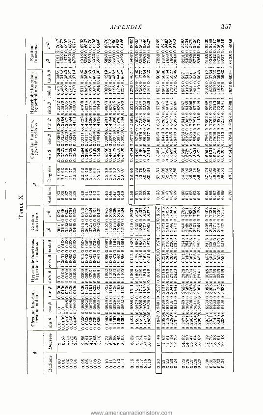
APPENDIX 357
Ó Ó
áU Ww
Ti,.
W
NNNO., MN000 1OM0000
NO00/0.0./. 0 ÑN ÓOC, 01C mM- t-00tCC tODOOOC 0t0O0c0
. . . . . . . . . . . . . . .
O O O O O O O O O O O O O O O
.00.00N 0 N100M 00dCO.0M 00N00 .0
Ó1,N Ñ Ó Ó CÓ0 N.000 1,1,MM Ñ+O D tCJ C 1CC7C OCCOC qLL40 d cocco C O O O O 0 0 0 0 0 O C O C O C
MNMO 00.0m. m-0.. CfMNNN -+ODNNN OOVCODN Md.tON 010NM0 OD000-+M 1,1,1,1,1, W10101g10 lOtOC00000 ..... ..... .....
.-. ..... ..... .. .. ..
N MOOC M NMOO 1,C0.010 OCWNCIN OC 00 1ON00c0 M 000tOW N000NO0 10Jy.MM M. W c000C1.-i M 1Ot000O NeMUJNO M10NC+ .0 cOOOtON N NNNW WWWWW Ó10000 c ..... ..... ..... .....
.
r -. .. .--i N -. -..-+ .. .. .-. -. -. -. ......
07
CO [
..0 Cd
b ...cCi
1.Ui .
A Nd A
Ql 1] g
w
1,01CN1, 000MO0 O..NNN .00C1,N-. CW.000M OW.0dO 0/1,100O0. WWOJ-. NCOC-0 0C CCMC+CMM MMM1,d 1,1,1,1, O O O O O cocco 0 0 0 0 0
-. ON1,C 10 01,N0 -0.. C: 1,C00C 1, N CN10M O W00N0 N1,-.W1, W10-+00 TM OO NNWO 00,-.NN M1,0Ct0e0 NNOOCICI O 1, 1,1,1,1, 10 10000JC0 1010101010 100J0J000J .0
Coco= C C C C C O O C C O C O C O C O C. CON-.0 -.N1001, CC-0.10 100MN 100M00 MNNNN n .0 .0=CONC.. W W W C O 00--N mO O O C O 0 0 0 0 0 U
OO OMW1, .00-- CMN N 0-.000-. WOCMCN 0
N40(0...... tL- O C0O - N M W ä 0 N N N N N N N N
^^.^ r
- dOCNOC N N1,^W I.-00,0C 000O 00CM.0- OD .-.NMOC.0 000-.M1, cD00001eM 000-.M.0 00 N M1,0C.0 0-W0.01 M1,.0NW OCNMeY 00 000,00 0C I000OOOO OOODOOODOD OONNNN N O C O C O cocco O C C C C C C C C O C
QQ. N000NO 00 .00 1,C9 Mä101,.. 00 NNW COO C-.01M1, +0ODN00C1
,.' OC.0NWO NM1,07 ONOOCCO MC+0MM1, 1,1,1,1,1, 1,1,1, M10
m 0 0 0 0 0 O 0 0 O 0 O O O C O .0 CC10C1 M cD.O-1CnIOD
C=CC-.10 N.MNM Cy: 0 d.00MO1, O.0NWOC N
1, OCNWO 011,10.0 000-.C11, .0NCCN 1, 00000 O0 .0.0.0.0 cOtONNN C- NNW W W
00000 0 0 0 0 0 COCCO O C O C O O
_
0 's
..1
D C w 4cl cl-.
74 íU. 'p Ú
Q1 0001,CN0-. Nd0D000 M01,C000OM .01-..W0-. NM1,0'1N WCONM MMMM1, 1,1,eM1,1, 1, 1,101010 O C O C O 00000 C O C C O
.0 N0000N 10 M010CC MNOC- CW.0M OC N NNNN 01N.-000 OCOCCWN cOOMN- 1, N N.0.000 1C 1,1,MM N.--.00 CCa1ooNN OD W WWWW W WWWOC WWWWW NNNNN N O 0000 O 0000 O O O O O 00000 C
1,aMNCC -.-.000 OC...0OM C. 0000NW1, -~.NMC1, Oc0-.NN
MC'CMNN N-.-.00 OCCC00000
Ó 00000 C1C1C1C1O OWWWOC 00000 0 0 0 0 0 00000 0C'OOOCIN 1,OOWCIO O0 710000
01 NN-.CO C100NC010 0]1,04.-.0 d00.0NW OOC10tiN M.1,0C.0N
C MMMMM MM1,d'1, 1,1,1,eM1, m co 0 0 0 coo O O O O O O O
.1.017/0--. N N.0O1, .000.-.N N-.CWCO N 00 W000C1, N 0W.0 .MN-.ON 10M.^OC.0 e1,
!..17,442:-7, N MM1,10 .0NW W0 C,-.NNM 1, C0 1q1q0010 1qC000J0J0C .0.0.0.0.0 .0
O cc co O C coo O C O C O cocco C
M.
U bMONOC NOCO1,-. W.0MON cU.
O.0NNM 01,0OON NMCCIOC o 00..-.N NM1,1,CO 10000DN00 Q N N N N N N N N N N 0101 N N N
10 NONeM C1OD1,0 WIONON e1,NC1tom .0 NNMO 10 00DN00 40010-..0 00M00 00 00000 1. NNMCC 1,d10.0.0 NN000001 O N Cl N M M M M M M M M M M M M 4140400/40 1,
g, 0C0DN00C 0.-.01 01 1, 000N000 40 0/0/(000 e1. 1,1,1,1, 1,1,1,1, 1,
-C1 ..... ..... ..... cl O O O O O 00000 O C 0 0 0 Qi
O..NMeN CO .01.-000 0.010/ .7. .0 .01,000/ 0 W 0C10C1000 0 1010/0/0 .0.0 000000 ODCOOOtDCD t- .... . .... ..... ..... .
O 0000 O 0000 O O O O O 00000 O
qm C.
0....C.;
D áC Ww
ON1,00 ^100.M..0 WOO O-.1, N-.NC'CO Ql 00000 - 1,hCOW0 C NCCO'CN
i 00WN.0 -- CCCWN.0 .0 0C1,MN v 000CCCC1 0= ___ OWWWW W WWWW
.0000 .0.00.00 00000 O O O O O
N.00'01t`.0 W C0
. 00000 1, -.
010/.4,0N N
1, NNODC010 CO -.
00000
00-.1,MCI 001,-.000 CN1,.0 W.-rM10W OMmW-. --COW NN.0C01, eMMN-.-. WWNN NNNNN NNNNN
.
O O C 0 0 00000 N-OON 000-1, 01,CC, MCOW- 1,000MCD OMN.-. WO-.NM dODNOn N N N N N N M M M M M M M d.
VOW r%^MN NMCOWM W OMNM 00000 --^M1, 0.0NW0 M0N0 Q1W OCC00 000000 O-.N-M.-CC. cO..N.W-O.N
..... 010010 0M000-. 40.7.0,0 .0 1,1,MNN COWN 0-C]M .000.0 0OC-C NNNN NNNNN NMMMM
O O O O O 00000
Q1 0000 OOOWW NOO1,C7-. Oct-.1.,-,00 COCO 00000 00000 W WWWN
yy .Nc0.4. 000.01..00 CO-.NM .1.07/NW C 00000 00000 O..-. ..... ÿ 00000 0 0 0 0 0 00000 O O O O O
C 0
cd
J.11
ro
U 2 C Ó .414 Dÿ O.a
.:'1'4.'
C. NOCW WON0.0.000 M WON. OCOO Nc1, Incr.-WC -NeMOW
O poop 00000 00000
C O 0 0 0 0 00000 O O O O O 0 0 0 0 0
. .
o ..... ..... -. -. -. . . .....
...MCC O N O ... M C N 00000 N-..0..N N O N 00000
..1.0C-0. 1, M1,0CCe N1,.0W 1,.0ON 0CW-0CW N N N N M M M M eM 1, 1, 0 0 0 O O C O 0 0 0 0 0 O O C C C
.. ..... ..... OCWOM COOMN.. 0CC000.0 NN NNMM1, 1,M 7.0.0 -.N M eM 00000.0000..00M 0 0.N0/.1, N N N N N N N N N M M M MM
0 0 0 0 0 00000
Q1 0000 CO... NNM1,0C OC NWON 0000 OOCOO 00000 000.. NM1, 000N000 O.NM 000.000
[ 0 0 0 0 0 O O O O O - y m 00000 O O O O O 00000 O O O O O
MOW.01, MM1,000N MM1,1, OCOCCCW OC-.NM
NMeM 10.0NW0 ONM1,0'0 NNNN NNNNN MMMC'0CC 00000 O C O O C
m CO
C . N E"'" 7w
7
00000 0-.-.NN 40ä000.0 ...,NOM Q1 OOOCO OCCOO 00000 NN
O-.NM1, 000CNW0 0..1 CO 00-0 ..00.1
00000 00000 -. .'. 00000 00000 00000 0 0 0 0 0
WOCN WNOCWO COCOON W NcCWO Ql =CC WWNC0c0 101,01-0 W N10MN 000 000C10 00000 W WWWW p 00000 00000 000M0 0.0=== ° .-.óóó 0..7..000 ó0000 0 0000
O W 0 0
OONM 01,0-.N MMNCW W0'CC'C.. WCDM..W CCNOCON NNNN c00000m10 0C0CeMeM1, C0000 00000 OOCCCO 0000 OOOó0 OOOóó
O00CCC1 00000-.000 1, MNOO C. 0000 00000 00000 O C0000W
NM1, 07000CNW OO-.NM 1, 1000W ,C, 00000 00000 O-...-.-. -. -. ---------- m 0 0 J 00 O O O O O C C O O O 000 0
N W O
00000
1001ON 1,-.N1,0 10.-..0010 WWWN NNOOmtC 10101,e1,M 0.-NM eM10OCNW OO..NCC 00000000 NNNNN NMMMM
00000 00000
OS
d 00.0-.-.NN W1,00C NM 00.1.0 1000 NNMW m U 00-.^N NMeM1,O 100DONW 00 =COCO .
1,
^ -'. C.0W0 NON1,N OC.0M-.W N M 0 1, O.0 .0-000.4.
NNM 1,1, COO WWO .--- g O-.NC'C1, 0 OCN00 O O-NM 100.0NW b 00000 00000 . ..-. C 00000 O O O O O 00000 O 0000 g
C-NC01, N 0
CC.0NWO O..NMeM NNNN NNNNN MMMMM 0000 O O O O O 00000
www.americanradiohistory.com

358 FREQUENCY MODULATION
It can be shown that for an open -ended feeder shorter than X/4 the line behaves like a condenser of quality
Zo sin ('2 l) lR (231)
where lis the actual length of the line in centimeters and S is the phase constant 27r /X. In a similar way a feeder short -circuited at the far end and shorter than X/4 acts at the input side like a coil with a quality
Z° sin (2U) - IR (232)
It can be shown that the input impedance Z, for a length I which is almost any integer multiple of X/2 such as X /2, X, 3X12, etc., and open at the far end i3
2Z° 1 (233) Z' IR 27rZo F Fr\ 1
7 XR \Fr - F
where Fr is the frequency that would cause exact line resonance and F is the operating frequency that produces almost line resonance for X/2 distributions. Hence, when we deal with exact line resonance conditions, as with tank feeders (feeder acting as a tank), we have F = Fr and Z, = Zr, or
2Z2 Zr =
IR° 271-Z0
XR
(234)
For the case of an open -ended line whose length l is almost any odd multiple of X /4, we have the input impedance
¡ l 1 2 L -h 3 2Ra ° (F -F / J (235) Z,_ 1
r
We have, therefore, the case similar to a series resonance circuit. Equation (235) holds not only for an open -ended line almost any odd multiple of X/4 long but also for any short -circuited line nearly any integer multiple of X /2.
70. Magnitudes of Important Factors.
/ Permeability µ = 47r X 10 -7 henrys /m
s
Dielectric constant K = 36 farads /m
In empty space
111
salt water (ocean)
Velocity of propagation c = 1 1
x/1.257 X 10-6 X 8.854 X 10 -12
= 2.998 m /sec
Natural impedance Zo = = 376.7 ohms
µd = Ft
Ks = 80K
c 2.998 C. = = m/sec
V80 V80
Natural impedance Z,, = V-- = z° = 376.7 80K
= 37.6 ohms
www.americanradiohistory.com

APPENDIX 359
With respect to Fig. 36a the ratio of the field strength of refracted wave to incident wave (T coefficient of refraction) depends on angles v. We have
2 cos yo sin y T sin (ç, + Y) cos (ç, - y)
sin w . I 2jo sin ry
K - F
www.americanradiohistory.com


REFERENCES In order to eliminate certain references in which the reader may not be interested,
the following are grouped according to their topics. The first group deals, for instance, only with publications having a bearing on the spectrum solution.
Publications on the Theory of the Distribution of the Modulation Energy in the Frequency Spectrum
VON HELMHOLTZ, H. L. F., On Sound Sensations ( "Lehre von den Tonempfindungen"), 1862 (Latest edi., 1913, Braunschweig, p. 649 -650, 1913).
RAYLEIGH, LORD JOHN WILLIAM STRUTT, Scientific Papers, Vol. 3, p. 1, 1887; Vol. 2, p. 88, 1883.
MATHIEU, E., Jour. de math. pures et appliquées, 13, p. 137, 1868. WHITTAKER, E. T., Proc. Edinburgh Math. Soc., 33: p. 22, 1914; 32, p. 75, 1914. CARSON, J. R., Proc. IRE, 10, p. 57, 1922. INCE, L. L., Proc. London Math. Soc., 23, (2), 56, 1925; Proc. Roy. Soc. (Edinburgh),
45, 106, 1925; Proc. London Math. Soc. 25, (2), 53, 1926. Pot., B. VAN DER, Exp. tireless, 1926; Proc. IRE, 18, 1194, 1930. POL, B. VAN DER, and M. J. O. STRUTT, Phil. Mag., 5, 18, 1928. ST7'UTT, M. J. O., Zeit. f. Phys., 69, 597, 1931; "Lamésche- Mathieusche -, und ver -
wandte Funktionen in Physik und Technik," Ergeb. der Math., Band I, Hirsch - waldsche Buchhandlung, Berlin, 1932.
HUMBERT, "Fonctions de Lamé et fonctions de Mathieu," Mémorial des Sc. Math., Vol. 10, Paris, 1926.
WINTER -GUENTER, H., Jahrb. der drahtl., 34, 1, 1929; 37, 172, 1931. SALINGER, H. ENT, 6, 294, 1929. BARROW, W. L., Ann. der Phys., 11, 147, 1931; Proc. IRE, 20, 1626, 1932. POINCARP, H., "Mécanique Céleste II," p. 253. WHITAKER and WATSON, Modern Analysis, Chap. IX.
Publications on the Theory of Wave Propagation in the FM Range of Carrier Frequencies
BEVERAGE, H. H., H. O. PETERSON, and C. W. HANSELL, Application of Frequencies above 30,000 Kilocycles to Communication Problems, Proc. IRE, 19, 1313, 1931.
ECKERSLEY, T. L., Short -wave Wireless Telegraphy, J.I.E.E. (London), 65, 600, 1927; Ultra -short Nave Refraction and Diffraction, J.I.E.E. (London), 80, 286, 1937.
JONES, L. F., A Study of the propagation of wave Lengths between Three and Eight Meters, Proc. IRE, 21, 349, 1933.
TREVOR, BERTRAM, and P. S. CARTER, Notes of Propagation of Waves below Ten Meters in Length, Proc. IRE, 21, 387, 1933.
SCHELLENG, J. C., C. R. BURROWS, and E. B. FERRELL, Ultra -short -wave Propaga- tion, froc. IRE, 21, 427, 1933.
ENGLUND, CARL R., ARTHUR B. CRAWFORD, and WILLIAM W. MUMFORD, Some Results of a Study of Ultra -short -wave Transmission Phenomena, Proc. IRE, 21, 464, 1933.
SMITH -ROSE, R. L., and J. S. MCPETRIE, Proc. Phys. Soc. (London), 43, Part 5, No. 240, 592, 1931.
361
www.americanradiohistory.com

362 FREQUENCY MODULATION
MUNRO, G. H., J.I.E.E. (London), 71, No. 426, 135, 1932. FELDMAN, C. B., The Optical Behavior of the Ground for Short Waves. Proc. IRE,
21, 764, 1933. BURROWS, C. R., A. DECINO, and L. E. HUNT, Elec. Eng., 54, 115, 1935; Proc. IRE,
23, 1507, 1935. VAN DER POL, B., and H. BREMMER, Phil. Mag., 24, 141, 826, 1937; Hochfrequenz-
technik und Elektroakustik, 51, 181, 1938; Report of Committee on Radio Wave Propagation, Proc. IRE, 26, 1193, 1938.
BURROWS, C. R., Radio Propagation over Plane Earth -field Strength Curves, Bell System Tech. J., 16, 45, 1937.
PETERSON, H. O., Ultra- high- frequency Propagation Formulas, RCA Rev., 4, 162, 1939.
CROSBY, MURRAY G., Frequency -modulation Propagation Characteristics, Proc. IRE, 24, June, 1936; The Service Range of Frequency Modulation, RCA Rev. 4, 349, 1940.
BEVERAGE, H. H., Some Notes o_n Ultra- high- frequency Propagation, RCA Rev., 1, January, 1937.
MACLEAN, K. G., and G. S. WICKIZER, Notes on the Random Fading of 50- megacycle Signals over Nonoptical Paths, Proc. IRE, 27, August, 1939.
WEIR, I. R., Comparative Field Tests of Frequency -modulation and Amplitude - modulation Transmitters, Proc. RCA, 16, July, 1939.
NORTON, K. A., Ground Wave Propagation, FCC, Fourth Annual Broadcast Engi- neering Conference, February 10-21, 1941, No. 47475; Report No. 48466 of FCC, Report prepared by K. A. Norton on the Effect of Frequency on the Signal Range of an Ultra -high Frequency Radio Station.
CROSBY, M. G., Observations of Frequency Modulated Propagation on 26 Mega- cycles, Proc. IRE, 29, 398, 1941.
EASTMAN, A. V., and J. R. WOODWARD, Binaural Transmission on a Single Channel, Electronics, 14, February, 1941.
GuY, R. F., and R. M. MORRIS, NBC Frequency Modulation Field Test, Radio Eng., 255, 12 -31, 136, January, 1941; Electronics, Reference Issue, June, 1941 (contains a very clear exposition for the entire field of FM in Sec. 3 consult also footnotes, p. 132).
BURROWS, HUNT, and DECINO, Ultra- short -wave Propagation: Mobile Urban Trans- mission Characteristics, Bell System Tech. J., 1935.
HANDEL, P. V., and WOLFGANG PFISTER, Ultra -short Wave Propagation along the Curved Earth's Surface, Hochfrequenctezhnik und Elektroakustik, 47, June, 1936.
HULL, Ross, Air -mass Conditions and the Bending of Ultra- high- frequency Waves, QST, June, 1935, p. 13.
HOLMES, R. S., and A. H. TURNER, An Urban Field Strength Survey, at Thirty and One Hundred Megacycles, Proc. IRE, May, 1936.
BURROWS, C. R., The Propagation of Short Radio Waves over the North Atlantic, Proc. IRE, Sept., 1931.
CARTER, P. S., and G. S. WICKIZER, Ultra High Frequency Transmission between the RCA Building and the Empire State Building in New York City, Proc. IRE, August, 1936.
BEVERAGE, H. H., Some Notes on Ultra -high Frequency Propagation, RCA Television, Vol. II, October, 1937, p. 98 (a reprint from RCA Rev., January, 1937).
Publications on Dipoles, other Antenna Systems and Feeders Employed in FM Work CARTER, P. S., Circuit Relations in Radiating Systems and Applications to Antenna
Problems, Proc. IRE, 20, 1004, 1932; see also footnotes on p. 285.
www.americanradiohistory.com

REFERENCES 363
I ItOWN, G. H., Directional Antennas, Proc. IRE, 25, 78, 1937; The Turnstile Antenna, Electronics, 9, 14, April, 1936.
AcEVES, J. G., Antennas for FM- reception, 14, 42, September, 1941.
LINDENBLAD, N. E., Antennas and Transmission Lines at the Empire State Television Station, Communications, 21, 10, April, 1941.
HARRIS, C. C., Losses in Twisted Pair Transmission Lines at Radio Frequencies, Proc. IRE, 24, 425, 1936.
WHEELER, HAROLD A., and V. E. WHITMAN, The Design of Doublet Antenna Systems, Proc. IRE, 24, 1257, 1936.
E. STMAN, A. V., and E. D. Scovv, Transmission Lines as Frequency Modulators, Proc. IRE, 22, 878, 1934.
RAKSKIT, H., Recent Technical Development in Wireless and Broadcasting in Great Britain, Science and Culture, 6, November December, 1940.
KRAUS, JOHN D., Multiwire Dipole Antennas, Electronics, January, 1940, p. 26.
BARBER, ALFRED W., Television Receiving Antennas and Transmission Lines, Com-
munications, February, 1940, p. 15.
RODER, HANS, Graphical Methods for Problems Involving Radio- frequency Trans- mission Lines, Proc. IRE, February, 1933, pp. 290 -302.
WHITHER, ROBERT, Radiation Resistance of Concentric Conductor 'transmission Lines, Proc. IRE, September, 1933, pp. 1343 -1353.
GOLDMAN, S., Dipoles and Reflectors, Electronics, May, 1940, p. 21.
BROWN, G. H., Vertical vs. Horizontal Polarization, Electronics, October, 1940, p. 20 (consult also: C. J. Young, Proc. IRE, 22, 1290, November, 1934, and C. N. Anderson and I. E. Lattimer, Proc. IRE, 20, 415, March, 1932); Electronics, Reference Issue, 14, June, 1941.
NERGAARD, L. S., and B. SALZBERG, Resonant Impedance of Transmission Lines, Proc. IRE, 27, 579, 1939.
SALZBERG, B., On the Optimum Length for Transmission Lines Used as Circuit Elements, Proc. IRE, 25, 1564, 1937.
LEEDS, L. A., Concentric Narrow- band -elimination Filter, Proc. IRE, 26, 576, 1938.
EVERITT, W. L., "Communication Engineering," McGraw -Hill Book Company, Inc., New York.
STEBBA, E. J., and C. B. FELDMAN, Transmission Lines for Short -wave Radio Systems, Proc. IRE, 20, 1163, 1932.
BROWN, G. H., and J. EPSTEIN, An Ultra -high Frequency Antenna of Simple Con- struction, Communications, 20, 3, July, 1940.
WINLUND, E. S., FM Engineering Considerations (Contains "Economics of Antenna Design "), FM, July, 1941, p. 23.
Publications on Noise and Interference Due to Noise
CARSON, JOHN R., Selective Circuits and Static Interference, Bell System Tech. J. 4,
(2) April, 1925; also in Electrical Communication, 3 (4) April, 1925; Reduction of
Atmospheric Disturbances, Proc. IRE, July, 1928, p. 967. ARMSTRONG, E. H., A Method of Reducing Disturbances in Radio Signalling by a
System of Frequency Modulation, Proc. IRE, May, 1936, p. 689. LANDON, V. D., A Study of Noise Characteristics, Proc. IRE, November, 1936, p. 1514.
CROSBY, M. G., Frequency -modulation Noise Characteristics, Proc. IRE, April, 1937,
p. 472. RODER, H., Noise in Frequency Modulation, Electronics, May, 1937, p. 22.
PLUMP, E. H., Reduction of Interference by Frequency Modulation, Hochfrequenz-
tecknik and Elektroakustik, September, 1938, p. 73.
www.americanradiohistory.com

366 FREQUENCY MODULATION
WINLUND, E. S., Drift Analysis of the Crosby Frequency- modulated Transmitter Circuit, Proc. IRE, 29, 390, 1941.
ARMSTRONG, E. H., Evolution of Frequency Modulation, Elec. Eng., 59, 485, Decem-
ber, 1940. CARSON, J. R., Amplitude, Frequency, and Phase Angle Modulation, Wireless Eng.,
17, 477, November, 1940. HUDEO, E., The Transmission of Pictures by Frequency Modulation, ENT, 18, 12,
January- February, 1941. HOWE, G. W. O., Frequency versus Amplitude Modulation, Wireless Eng., 18, 1,
January, 1941. NORTON, L., Why Not Narrow Band FM for General Amateur Use ?, Radio, 88 -92,
152 -153, 159, January, 1941.
SPRAYBERRY, F. L., Principles of Frequency Modulation Part II, Radio and Telev.,
11, 744, April, 1941. WEISS, W., Detection in Frequency Modulation Receivers, Communications, 21,
16, 18, March, 1941; Amplitude, Frequency and Phase Modulation, Letter to
Editor, Wireless Eng., 17, 441, October, 1940.
WHEELER, H. A., Two -signal Cross Modulation in a Frequency Modulation Receiver, Proc. IRE, 28, 537, December, 1940.
BARROW, W. L., A New Electrical Method of Frequency Analysis and Its Application to FM, Proc. IRE, 20, 1626, 1932.
CHAFFEE, J. G., The Application of Negative Feedback to FM Systems, Bell System
Tech. J. 404, October, 1937; Proc. IRE, 317, May, 1939.
Yocum, C. H., Frequency Modulated Transmitters, Communications, November, 1939, p. 5; Electronics, November, 1939, p. 20.
FINK, D. G., Phase -frequency Modulation, Electronics, November, 1935, p. 431.
CARSON and FRY, Variable -frequency Electric Circuit Theory with Application to the Theory of FM, Bell System Tech. J., October, 1937, p. 513.
WOODYARD, J. R., Application of the Autosynchronized Oscillator to Frequency Demodulation, Proc. IRE, May, 1937, p. 612.
WEIR, I. R., Wide Band FM vs. AM for Aircraft, Electronics, November, 1940, p. 34; Synchronized Frequency Modulation, Communications, 20, 12, August, 1940.
CROSBY, M. G., A Method of Measuring Frequency Deviation, RCA Rev., 4, 473,
April, 1940.
Publications on Apparatus Employed in FM Transmitters and Receivers
DAY, J. R., A Receiver for FM, Electronics, .June, 1939, p. 32. BARBER, A. W., Frequency Modulated Generators, Radio Eng., November, 1936, p. 14. EASTMAN, A. V., and E. D. SCOTT, Transmission Lines as Frequency Modulators,
Proc. IR.E, July, 1934, p. 878. TRAVIS, CHARLES, Automatic Frequency Control, Proc. IRE, 23, 1125, 1935. MILLER, R. L., Fractional- frequency Generators Utilizing Regenerative Modulation,
Proc. IRE, 27, 446, 1939. NYQUIST, H., Regeneration Theory, Bell System Tech. J., 11, 236, 1932. HORTON, J. W., U. S. Patent, No. 1690299. STERKY, H., Frequency Multiplication and Division, Proc. IRE, 25, 1153, 1937. GROSZxowsKI, J., Frequency Division, Proc. IRE, 18, 1960, 1930. KOGA, I., A New Frequency Transformer or Frequency Changer, Proc. IRE, 15, 669,
1927. RODER, H., Theory of the Discriminator Circuit for Automatic Frequency Control,
Proc. IRE, 26. .590, 1938.
www.americanradiohistory.com

REFERENCES 367
FOSTER, D. E., and S. W. SEELEY, Automatic Tuning, Simplified Circuits and Design Practice, Proc. IRE, 25, 289, 1937.
RODER, H., Some Notes on Demodulation, Proc. IRE, 20, 1946, 1932.
SIIEAFFER, C. F., Frequency Modulator, Proc. IRE, 28, 66, February, 1940.
PIERACCI, ROGER J., A Frequency -modulation Monitoring System, Proc. IRE, 28,
374, 1940. NOBLE, D. E., A State -wide FM Police System, Electronics, November, 1940, p. 18;
December, 1940, p. 28. DAVID, W. R., FM Broadcast Transmitters, Communications, 20, 8, October, 1940.
HOBBS, M., FM Receivers -Design and Performance, Electronics, August, 1940, p. 22.
SHEA, R. F., Frequency Modulation Receiver Design, Communications, 20, 17, June, 1940.
CROSBY, M. G., Reactance Tube Frequency Modulators, RCA Rev., 5, 89, July, 1940.
BUDELMAN, F. T., 2 -way Link FM Data (circuit analysis of 25 -UF1\1 transmitter and 11 -UF receiver), FM, June, 1941, p. 24.
BROWNING, GLENN H., FM Service Instruments and Alignment Procedure, FM, June, 1941, p. 29.
LEVY, M. L., FM -AM Engineering Data (explaining the circuit design details and performance of the Stromberg- Carlson model 535 three -unit FM -AM receiver), FM, March, 1941, p. 8.
JAHNS, EDWARD, New Pilot A -FM Features, FM, July, 1941, p. 30.
THOMAS, H. P., and R. H. WILLIAMSON, A Commercial 50- kilowatt Frequency - modulation Broadcast Transmitting Station, Proc. IRE, 29, 537, October, 1941.
MORRISON, J. F., A New Broadcast Transmitter Design for Frequency Modulation, Proc. IRE, June, 1940. Also, a reprint by the Western Electric Company.
FOSTER, D. E., and JOHN A. RANKIN, Intermediate -frequency Values for Frequency Modulated -wave Receivers, Proc. IRE, 29, 546, October, 1941.
RICE, HARRY E., Factory Alignment Equipment for Frequency- modulation Receivers, Proc. IRE, 29, 551, October, 1941.
MONTGOMERY, BRUCE E., Air Inductively Coupled Frequency Modulator, Proc. IRE, 29, 559, October, 1941.
HALL, E. L., 30 to 340 Mc- wavemeter, Electronics, May, 1941, p. 37.
WEIR, I. R., Operating Problems in Frequency -modulation Transmitters, Com-
munications, 21, 5, May, 1941.
DAVID, W. R., G.E. Perfects FM Station Monitor, FM, 43, April, 1941; A Review of the Current A -FM Receiving Sets, FM, 12, May, 1941.
THOMAS, H. P., FM Measurements (outlines methods of measuring performance of
FM transmitters and of making determinations of field strength), Electronics,
July, 1941, p. 36. HOBBS, M., A Demonstration System for Frequency Modulation, Electronics, 20,
January, 1941. WEIR, I. R., Operating Problems in Frequency -modulated Transmitters, Com-
munications, 21, 7, June, 1941. LEVY, M. L., Frequency -modulation Receivers, Communications, 21, 5, March, 1941.
Frequency -modulation Transmitters, Communications, 21, 8, March, 1941.
TAYLOR, S. GORDON, AM /FM Broadcast Tuner, Communications, 21, 10, March, 1941.
WING, A. K., and J. E. YOUNG, A Transmitter for Frequency -modulated Broadcast Service Using a New Ultra- high- frequency Tetrode, RCA, Rev., 5, 327, January, 1941.
THOMAS, H. E., The Development of a Frequency Modulated Police Receiver for
Ultra- high- frequency Use, RCA Rev., 8, 222, October, 1941.
www.americanradiohistory.com
368 FREQUENCY MODULATION
HALLER, CECIL E., The Design and Development of Three New Ultra- high- frequency Transmitting Tubes, Proc. IIhE, 30, 20, January, 1942.
BARBER, A. W., C. J. Franks, and A. G. RICHARDSON, A Frequency Modulated Low Signal Generator, Electronics, 36 -38, 92 -95, April, 1941.
CROSBY, M. G., Tuned Filter for Frequency Modulation Defection, Electronics and Telev. and Short Wave World, 13, 486, November, 1940.
GI Y, R. F., and R. M. MORRIS, NBC Frequency Modulation Field Test, Radio, 12 -31, 136, January, 1941.
MUNIZ, R., D. OESTREICHER, and W. OESTREICHER, A pull -swing Frequency Modula- tion System for the Amateur, Radio and Telev., 11, 598, February, 1941; 12, 96, June, 1941.
SPRAYBERRY, F. L., Frequency Modulation Receivers, Radio and Telev., 12, 294, September, 1941.
THOMPSON, R. T., An 8 -tube Converter for FM Reception, Radio, 9, 70, 72, 74, March, 1941.
TooMSs, A., The Radio Battle of 1941, FM vs. AM, Radio News, 24, 43, March, 1941.
www.americanradiohistory.com

INDEX A
Accentuation (audio frequency), 11, 76, 121, 128, 219, 221, 236
Actions, in amplitude limiter, 105 (Fig. 28), 91, 209, 259, 276
in accentuator, 96, 121, 128, 219, 221, 236
in Armstrong system, 1, 3, 7, 36, 38, 44, 45, 77, 81, 121, 188, 231
in deaccentuator, 96, 210, 219, 221, 256, 265
in discriminator, 78, 193, 207 in frequency demodulation, 78, 193 in frequency modulation, 3, 14, 155 in phase demodulation, 78, 193, 225 in phase modulation, 3, 9, 225
Advance of phase, 2, 6, 9, 12, 45, 108, 111
Aerials (see antennas) Alignment, of converter, 253, 264
of discriminator, 207 of FM receiver, 264 of h -f stages, 266, 268 of i -f stages, 266, 268, 271
AM FM, 40, 63 AM + PM, 55 AM + PM + FM, 42, 69 Amplitude, carrier, 2, 3, 7
instantaneous value, 2, 3, 7, 8 limiter, 7, 63, 83, 92, 105 modulation, 3, 7 swing (deviation), 3, 9
Allocations of FM stations, 131, 249 Angle, of line, 309, 311, 313
of phase, 2, 3, 6, 9, 12, 45, 108, 111 of reflection, 133, 138, 143, 358
Angular velocity, of carrier, 2
of deviation, 2 of signal, 2
Antennas, receiver, 278, 294 reflector, 295 transmitter, 278, 334, 339 turnstile, 341
Apparent PM, 1, 45 Armstrong system, 1, 3, 7, 36, 38, 44,
45, 77, 81, 121, 188, 231
Armstrong transmitter, 121, 188, 231 Ascending electromagnetic ray, 133, 138,
143 Assignments, frequency of, 131, 249 Attenuation, line, 307, 315, 321, 328 Audio -frequency accentuation (pre -
emphasis), 96, 221 deaccentuation (de- emphasis), 96, 221
Automatic Bessel current suppression, 23, 41, 86
carrier suppression, 23, 86, 151, 153 center -frequency control, 127, 128,
205, 236, 239, 242 lower side -current suppression, 41
B
Backfeed, for center -frequency control, 128, 236
for regenerative modulation, 154, 155
Balanced amplitude modulator, 1, 150, 183, 185, 187
frequency modulator, 153, 175, 179 tube circuits, 151
Band -restriction filter, 90 Band width, 25, 48, 88, 99
comparison with deviation, 31, 33 design, 28, 33, 93, 203
Beat frequency, 93, 101
Beat interference, 93, 101
Bessel curves, 23, 25, 32, 86 distribution, 17, 21, 26, 30, 31, 33, 34,
44, 51, 58, 59, 347 distribution feature, 51 formulas, 17, 50, 56, 57, 61, 65, 70,
347 -355 functions, 17, 19, 23, 25, 32, 352, 353 tables, 19, 20, 24, 33, 353 theorem, 347 -355
Bridge circuits, 150, 151, 153, 155 369
www.americanradiohistory.com

370 FREQUENCY MODULATION
C
Capacity injection, 165, 166, 179 Carrier, current, 2, 3, 6, 8
deviation, 3, 8 frequency, 2 level, 3, 8, 45, 46 reinserted, 121, 185' suppressed, 23, 86, 151, 153
Center frequency, 3, 11, 14 modulation, 14, 155 -182 stabilization, 127, 128, 205, 236, 239,
242 Characteristic, Bessel function, 23, 25,
32, 86 demodulator, 78, 83 discriminator, 78, 83, 196, 199, 203, 208 frequency distribution (see Bessel dis-
tribution) limiter, 209, 211, 259 modulator (class A), 160 natural impedance, 300, 358 resonance, 257, 258, 267 selectivity, 257, 258
Ci curves, 282 Ci functions, 281, 354, 355 Comparison, of AM and FM, 17, 39, 63
of AM and PM, 17, 55 of AM, PM, and FM, 42, 69
Conductivity, 134, 137 Continuous spectrum, 19 Conversion, of FM into AM and audio,
78 into phase variations, 75 of PM into AM and audio, 78, 83 of signal into frequency variations, 75
Converter, 121, 128, 233, 236, 239, 251, 252
Coupling, interstage, 252, 253, 256 Cross -spectrum modulation, 59 Current, instantaneous value, for AM, 3,
8, 37, 39, 45 for FM, 3, 14, 16, 17, 37, 39, 45 for PM, 3, 10, 16, 17, 37, 45 limiter, 209
Current distribution, in frequency spec- trum (see Bessel distribution)
along lines, 305, 317, 318 Curves, attenuation, 258, 262, 322
Bessel, 23, 25, 32, 86 cosine, 3 integral cosine, 282
Curves, integral epsilon, 287 integral sine, 282 reactance, 288 resonance, 257, 258, 267 selectivity, 257, 258 sine, 3
D
AF (frequency deviation), 3, 5, 13, 31 -33, 36, 37, 44, 45, 69, 72, 83
AO (phase deviation), 3, 6, 12, 13, 25, 30, 32, 33, 36, 37, 45, 56, 72
OF and M interrelation, 33, 36, 37 Deaccentuation, 96, 221 Deemphasis, 96, 221 Degree, of amplitude modulation, 2, 6,
8, 38, 40, 48, 65, 68, 96, 107 of frequency modulation, 15, 155 -181 of phase modulation, 6, 10, 182
Demodulation amplitude, 3, 68, 99 frequency, 78, 193 phase, 78, 193
Design for bandwidth, 25, 28, 33, 93, 203 Determination, of AM, 2, 8, 42
of M', 40, 72, 85, 86 of M, 72, 85
Dielectric constant, 134, 136, 137, 358 Difference, between AM and FM, 3, 18,
39, 44, 45, 56, 69 between AM and PM, 3, 44, 45, 56, 69 between PM and FM, 3, 6, 13, 29, 45,
69 Differentiator frequency, 79, 193 Differentiator phase, 79, 193 Dipole, 279, 282, 284, 288, 294 -299, 305,
333 -342 Direct frequency modulation, 27, 75,
155 -181 current output of discriminator, 197 ray (wave), 133
Discriminator, frequency, 79, 197 -209 phase, 79, 193 tests, 207
Distance in wave propagation, 133 -149 Distribution, of current along lines, 305,
317, 318 of current in frequency spectrum, 17,
21, 26, 31, 33, 34, 44 of modulation energy, for AM, 9, 44
for FM, 17, 21, 26, 31, 33, 34, 44 for PM, 17, 21, 26, 30, 32, 33, 34
www.americanradiohistory.com

INDEX 371
Distribution, of voltage, 305, 317, 318 Division of frequency, and deviation fre-
quency, 122, 154, 242
Downcoming electromagnetic wave (ray), 133
E
Effective current, 46 height, 137, 289 length, 289
Ei curves, 287
Ei functions, 287, 354, 355
Electromagnetic and electrostatic units, 134, 136, 137
Electromagnetic mirror, 138 -144 Electromagnetic transparency, 138 -144 Emphasizer (audio frequency), 221
Epsilon functions, 356, 357
Equivalent frequency modulation, 6, 33,
43, 101 frequency swing, 43, 45, 57, 78, 107
phase modulation, 33, 36
phase swing, 15
Excitation of dipoles, 288, 305, 334, 338
Experimental test, for, AF, 16, 78
for M, 68, 71
F
Features, of AM, 7 of FM, 14 of PM, 9
Feeder, 299 Field intensity, 133 -149 Filter (RC), 236
Filter (slope), 83
Fluctuation noise, 100
Formula, decibel loss, 303, 304, 307, 308
deviation -frequency multiplication, 36
field intensity, 142, 143
group velocity, 312 input impedance, 315 instantaneous current, 2, 8, 10, 14-17 mutual impedance of antennas, 286
phase multiplication, 36, 37
phase velocity, 312 reactance, 288 resistance, 288 self -impedance of antennas, 281
surge impedance of lines, 300
FM allocation, 131, 249 definition, 1
degree of, 15
features, 14
receiver, 249 transmitter, 226
Franklin serial, 342 Frequency, audio, 2
carrier, 2
center, 3, 11, 14
demodulator (differentiator), 79, 193
deviation, 2
discriminator, 79, 193
division, 122, 154 excursion (see Frequency, deviation) flutter, 4, 12, 107
i -f, 249 instantaneous value, 3, 11, 14, 44, 45
multiplication, 121, 124, 226, 236, 239,
242 signal, 2
spectrum, 1, 9, 17, 21, 26, 28, 30, 31,
33, 34, 44, 88 spread, 1, 9, 17, 21, 26, 28, 30, 31, 33,
34, 44, 88 stabilization, 127, 128, 205, 236, 239,
242 swing (see Frequency, deviation)
Functions, Bessel, 17, 19, 23, 25, 32, 352,
353 cosine, 356, 357 epsilon, 356, 357 hyperbolic, 356, 357 integral epsilon, 287, 354, 355 integral cosine, 281, 354, 355 integral sine, 281, 354, 355 Mathieu, 349 Riccati, 350
Fundamental relations, for AM, 7
for FM, 14 for PM, 9
Fundamental resonance, along lines and antennas, 318, 320
G
g,, (mutual conductance), 160
General Electric transmitter, 235
Ground dielectric constant, 134, 136, 137,
358 electromagnetic propagation, 133
reflection, 133
www.americanradiohistory.com

372 FREQUENCY MODULATION
Ground dielectric constant, refraction, 133, 358
propagation, 133 transparency (electric), 138 -144
Group velocity, compared with phase velocity, 312
H
Half -wave dipole, 279, 282, 284, 288, 294 -299, 305, 333 -342
Half -wave line, 311 Harmonic distortion, 6 Height, actual, 133, 138
apparent, 133, 138, 142, 143 effective, 137, 289
Heterodyne action, 42, 71, 93, 101, 126 Horizontal dipole, 132, 140, 144 Horizontal polarization, 132, 140, 144
I
i -f alignment, 266 coupling, 266 frequencies, 259 -264 stages, 266
Image response, 259 Impedance, of dipoles, 281
of lines, 315 mutual, 286 self -, 281
Impulse noise, 100 Index of modulation, 17
of refraction, 135 Indirect FM, 3, 7, 11, 36, 77, 81
frequency transmitter, 92 PM, 1, 6 ray, 133
Injection, of capacitance, 166 of impedance, 161 of inductance, 166 of reactance, 156 of resistance, 161
Input impedance, of lines and dipoles, 281, 288, 315
Input stage (i -f), of discriminator, 197, 199
Insertion loss, 307 Instantaneous current, 3, 8, 16, 17, 37,
39, 45 frequency, 3, 11, 14, 44, 45 phase, 3, 9, 11, 45
Integral functions, 281, 287, 354, 355 Integral graphs, 282, 287, 354, 355 Interaction loss, 308 Inteference, and elimination, 92
modulation in AM receiver, 92, 95, 100, 109
modulation in FM receiver, 92, 95, 100, 109
Interstage coupling, 252, 253, 256 Inverse frequency and networks, 36, 45,
77, 81, 223 Inverter (phase), 179
J
J(0) curves (see Bessel curves) functions (see Bessel functions) tables (see Bessel tables)
K
K, degree of amplitude modulation, 2, 6, 8, 38, 40, 48, 65, 68, 96
K0, effective degree when several types of modulations are present, 40, 72
L
Lag line, 309 phase, 2, 6, 12, 91, 105, 108, 309 time, 2, 6, 12, 91, 105, 108
Lecher wire, 300 Limiter, amplitude, 7, 63, 83, 92, 105
characteristics, 209, 211, 259 current, 209, 211, 259 one -stage, compared with double -
stage, 211 voltage, 209, 211, 259
Linear conductor, 334, 356, 358 Lines, angle, 309
closed, 311 concentric, 300 constants, 309 exponential, 337 half wave length, 318 loss, 328 measurements, 308 open, 315, 318, 320, 325 parallel, 300 Q- value, 337, 356, 358 quarter wave length, 318 shorted, 315, 318, 320, 325 termination, 308
www.americanradiohistory.com

INDEX 373
Loss, attenuation, 316, 328 insertion, 307 interaction, 307 reflection, 307
M
Matching conjugate, 302, 304 general conditions, 302, 304 lines, 311 sections, 335, 336
Mathieu function, 349 Maximum amplitude deviation, 3
deviation ratio, 32 frequency deviation, 3, 5
compared with required band width, 5, 31, 33
phase deviation, 3 phase -swing multiplication, 37 permissible frequency deviation, 4
permissible phase swing for no distor- tion, 6, 36
Mean carrier frequency, 85 Measurement, of attenuation constant,
308 -333 of degree of AM, 2, 40 of degree of FM, 40, 72, 86 of degree of PM, 72
of propagation constant, 308 -333 of spectrum spread, 88
Mismatch, 301 Modulation, cross spectrum, 59
direct, 7, 235 -248 distribution, 9, 17, 21, 26, 30-34, 44 due to two unmodulated carriers, 92,
101, 105 energy, 5, 9, 17, 21, 26, 30, 31, 33, 34,
44, 51 equivalent, 6, 7 features, of AM, 3, 7
of FM, 3, 14, 51 of PM, 3, 9, 51
harmonic, 8, 14, 16, 17 indirect, 7, 131 index, 17 one type, 3, 7, 9, 14 products, 1, 6, 8, 37, 38, 49, 60, 67, 69 saw tooth, 88 several types, 40, 42, 55, 63, 69
Modulator, amplitude, 150 balanced, 150, 153, 175, 179 frequency, 155
Modulator, phase, 182 reactance tube (principle), 155
Multiplication, of carrier frequencies, 118 of deviation frequencies, 118
D1utual conductance, 160 Mutual impedance, 286
N
Natural impedance, in empty space, 358 of lines, 325 in water, 358
Networks, accentuator, 223 deaccentuator, 223 discriminator, 196, 197, 199, 205, 207,
208, 210 i -f, 253, 256, 265 inverse frequency, 223 limiter, 210, 211
Noise, 92 fluctuation, 51, 92, 100 random, 92 shape, 95
O
Open -ended line, 315 Optimum feeder dimensions, 300, 355,
356
P
PM (equivalent), 11
PM features, 3, 9 PM + AM, 55 PM + FM + AM, 42, 69 Parasitic modulations, 1, 41
Permeability, 358 Phase angle (see Angle, of phase)
demodulator, 78 deviation, 3, 13, 26, 30, 33
distribution, 16, 30 excursion, 3, 6, 9, 12, 13, 16, 26, 30, 33,
36 fixed, 2, 9, 10 flutter, 4, 12, 28, 107 instantaneous value, 3, 10, 45 inversion, 179 modulator, 182 shifter, 39 swing, 3, 36 swing multiplication, 36, 37 velocity, 312
www.americanradiohistory.com

374 FREQUENCY MODULATION
Phase modulation, degree of, 10 instantaneous current value, 10, 16,
17 spectrum distribution, 17, 26, 30 spectrum distribution in comparison
with FM, 30, 31 Piezo generator (stabilization), 121, 128,
236, 239, 242 Plate limitation, 209 Polarization, horizontal, 131, 139, 144
vertical, 131, 139, 144 Preaccentuator (preemphasis), 221 Predistorter, 121 Product (modulation), 1, 6, 8, 37, 38, 49,
60, 67, 69 Propagation, in any medium, 135
constant, generalized angular velocity n, 315
wave, 131
Q
Q value of lines, 355 -356 Quadrature modulations, 3, 5, 155 Quadrature tube, 162 Quarter wave lines, 311
R
Radiation, formulas, 142, 143, 149 impedance, 288 resistance, 288
Random noise, 51, 92 Ray, direct, 133
indirect, 133 RCA transmitter, 240 Reactance, of dipole, 288
injections, 156, 161, 166 of line, 315, 318, 356, 358 modulators, 155 tubes, 155
Receiver, antennas, 278 current, 281 FM, 249 PM, 225 superheterodyne, 88 tests, 207, 264
References to FM publications, 359 Reflection, coefficient, horizontal, 139,
144 vertical, 139, 144 of waves, 139
Reflector antenna, 295 Refracted wave, 133, 358 Refraction, 133, 358
index of, 135 Regenerative modulation for frequency
division, 154 Reinsertion of carrier, 121, 185 Resistance, of dipole, 288
of line, 315, 319 Response, image, 259 Restriction of band width, 90 Retardation of phase, 9, 45 Riccati function, 350 Ring modulator, 152
S
Self- impedance, 281 Side currents, 4, 9, 17, 21, 26 Side frequencies, 4, 9, 17, 21, 26 Signal current, 2, 75
frequency, 2 generator (FM), 245
Slope characteristic, 83 Specific conductivity, 134, 137 Spectrum, 17, 21, 26, 30, 31, 34, 44, 50,
350 Spectrum distribution, AM, 9, 17, 21,
26, 30, 31, 33, 350 FM, 17, 31, 44 PM, 17, 30
Spectrum frequencies, 9, 17, 21, 26, 30- 33
Spectrum theory, 347 Stabilization, of the center (carrier) fre-
quency, 127, 128, 205, 236, 239, 242 electronic, 236 mechanical, 242
Static interference elimination, 85 Superheterodyne, 88 Superposition of two currents, with
modulation, 108 with no modulation, 101
Suppression, of carrier current, 23, 86, 150
of side current, 23, 40 Surge impedance, of concentric line, 300
of empty space, 358 of lines, 299 -333 of parallel wires, 300 of water, 358
www.americanradiohistory.com

INDEX
Swing amplitude (i,,,), 3, 8
frequency (SF), 3, 14
phase (SO), 3, 10
T
Tables, Bessel, 19, 20, 24, 33, 352, 353 cosine, 356, 357 epsilon, 356, 357 hyperbolic, 356, 357 integral cosine, 354, 355 integral epsilon, 354, 355 integral sine, 354, 355 sine, 356, 357 trigonometric, 356, 357
Terminations, conjugate, 304 matched, 299 -308 for maximum power transfer, 304 mismatched, 299 -308 for no reflections, 304
Tests, alignment, 207, 264 converter, 264 discriminator, 207 on feeders, 299 -321, 322 i -f stages, 264 limiter, 264
Threefold modulation, 42, 69 Time constant, 212
delay, 212 phase, 2, 3, 6, 9
Translation of, AM into audio, 197
current (or voltage), into FM, 75, 155
into PM, 75, 182
375
Translation of, FM into audio, 78, 197
PM into audio, 78, 225 Transmitters, direct FM, 227, 235 -248
indirect, 227, 231 Trigonometric tables, 356, 357 Tuned circuits, 195 -197 Turnstile antenna, Brown, 342
General Electric Co., 344 Twofold modulation, 40, 55, 63 Types of modulation, 3
U
Undesired modulations, 1, 41
V
Velocity, group and phase compared, 312
Voltage, audio of discriminator, 197
direct voltage of discriminator, 197
distribution, 330 limitation, 209
W
Wave propagation, 131
Western Electric Company, electro- mechanical center -frequency control direct FM Transmitter, 123 -126, 242
Wide -band FM, 4 Width of band, 25, 48, 88, 99
www.americanradiohistory.com
