friction and wear behaviour of self lubricating …
TRANSCRIPT
i
FRICTION AND WEAR BEHAVIOUR OF SELF
LUBRICATING BEARING LINERS
Russell Gay
Thesis submitted in candidature
for the degree of Doctor of Philosophy
at Cardiff University
Tribology Group
Institute of Theoretical, Applied and Computational Mechanics
Cardiff School of Engineering
Cardiff University
March 2013

ii
Declaration
This work has not previously been accepted in substance for any degree and is not being concurrently submitted in candidature for any degree.
Signed ________________________ (candidate)
Dated _____________
Statement 1
This thesis is being submitted in partial fulfilment of the requirements for the degree of PhD.
Signed ________________________ (candidate)
Dated _____________
Statement 2
This thesis is the result of my own independent work / investigation, except where otherwise stated. Other sources are acknowledged by explicit references.
Signed ________________________ (candidate)
Dated _____________
Statement 3
I hereby give consent for my thesis, if accepted, to be available for photocopying and for inter-library loan, and for the title and summary to be made available to outside organisations.
Signed ________________________ (candidate)
Dated _____________
iii
Summary
The thesis describes a numerical model for evaluating the variation of friction and wear of a
self lubricating bearing liner over its useful wear life. Self-lubricating bearings have been in
widespread use since the mid-1950s, particularly in the aerospace industry where they have
the advantage of being low maintenance components. They are commonly used in relatively
low speed, reciprocating applications such as control surface actuators, and usually consist of
a spherical bearing with the inner and outer elements separated by a composite textile resin-
bonded liner.
A finite element model has been developed to predict the local stiffness of a particular liner at
different states of wear. Results obtained using the model were used to predict the overall
friction coefficient as it evolves due to wear, which is a novel approach. Experimental testing
was performed on a bespoke flat-on-flat wear test rig with a reciprocating motion to validate
the results of the friction model. These tests were carried out on a commercially-available
bearing liner, predominantly at a high contact pressure and an average sliding speed of 0.2
ms-1. Good agreement between predicted and experimentally measured wear was obtained
when appropriate coefficients of friction were used in the friction model, and when the
reciprocating sliding distance was above a critical value.
A numerical wear model was also developed to predict the trend of backlash development in
real bearing geometries using a novel approach. Results from the wear model were validated
against full-scale bearing tests carried out elsewhere by the sponsoring company. Good
agreement was obtained between the model predictions and the experimental results for the
first 80% of the bearing wear life, and explanations for the discrepancy during the last 20% of
the wear life have been proposed.

iv
Acknowledgments
A large amount of the credit for this thesis is due to my two excellent supervisors, Professor
Pwt Evans and Professor Ray Snidle of Cardiff University, both of which have been brilliant
to work with over the last four years. They have helped me develop my skills as a researcher,
an engineer, and as a project supervisor, invaluable experience I will always be able to call
upon.
My thanks are due to the EPSRC who funded this project through a joint CASE award with
SKF, who also funded my travel to SKF research centres throughout Europe. I would like to
thank Andy Bell, Paul Hancock and Michael Colton from SKF Aerospace with whom it has
been a pleasure to work. I would also like to thank members of the SKF MFSC Workgroup
who have been both friendly and very helpful over the duration of this project.
I must thank my friends Michael Bryant and Grant Dennis for keeping me sane for the last
few years, and thanks also to my colleagues Amjad Al-Hamood, Anton Manoylov, Ingram
Weeks, Dr. Ben Wright, Matteo Carli, Dr Kayri Sharif and Dr. Alastair Clarke, of the
Tribology Group. In addition, thank you to the Cardiff Racing Formula Student team, who
have on many occasions given me a welcome distraction from my work, and the entire UCAS
team, who have provided both fun and frustration in equal measure.
A special thank you to my parents for their support throughout all my studies, and to my
family for their encouragement. Finally I wish to thank my friends - Marc, Charlie, Andy,
Josh, James, Robin, Mike, Hesky, and my girlfriend, Lucy, for not only looking after me over
the last four years, but also making my time in Cardiff so memorable.

v
Contents
Declaration ii
Summary iii
Acknowledgments iv
Chapter 1: Introduction and Review of Relevant Work
1.1 Overview 1
1.2 Tribology and Self-Lubricating Bearings 1
1.3 History of Textile Liners 9
1.4 Woven Fabric Bearing Liners 12
1.4.1 Performance of Polymer Self-Lubricating Bearings 13
1.4.2 Counterface 18
1.4.3 Bearing Geometry 19
1.4.4 Environmental Conditions 21
1.5 Tribology of Dry Sliding 25
1.6 Computer Modelling of Self-Lubricating Bearings 30
1.7 Future Development of Bearing Liners 34
1.8 Aims & Objectives 35
Chapter 2: Modelling the Weave
2.1 Objectives 37
2.2 Weave Visualisation 39
2.3 Finite Element Model 40
2.3.1 Unit Cell Geometry 40
vi
2.3.2 Contact Settings and Element Selection 49
2.3.3 Harmonic Boundary Conditions 58
2.4 Assumptions and Limitations 65
2.4.1 Thread Cross-Sections 65
2.4.2 Variation in Thread Thickness 67
2.4.3 Weave Pattern in Warp vs. Weft Direction 67
Chapter 3: Building the Weave Model
3.1 Overview 69
3.2 Python Script Structure 71
3.2.1 User Variables 71
3.2.2 Abaqus General Commands 72
3.2.3 Create Design Area 73
3.2.4 Model Assembly 78
3.3 Post-Python Tasks 80
3.4 Results 82
3.5 Technicalities of Python Script 84
3.5.1 Selecting Points 84
3.5.2 Mesh Resolution 85
3.5.3 Omission of Prepreg Layer 88
Chapter 4: Friction Model
4.1 Concept Overview 93
4.2 Tribology Assumptions 94
4.3 Principles 96
4.4 Abaqus Output Files 98

vii
4.5 Wear Steps 102
4.6 Model Structure 104
4.6.1 Model Setup 105
4.6.2 Load External Inputs 106
4.6.3 Format Data 107
4.6.4 Define Materials 108
4.6.5 Calculate Friction Coefficients 108
4.7 Results 110
4.8 Limitations 114
Chapter 5: Experimental Work & Comparison to Friction Model Results
5.1 Overview 117
5.1.1 Capabilities 118
5.1.2 Key Features 119
5.1.3 Data Output 125
5.1.4 Early Test Rig Problems 126
5.2 Test Results 128
5.2.1 Example of Test Results 128
5.2.2 Variation in Reciprocating Sliding Distance 136
5.2.3 Variation of Mean Contact Pressures 144
5.2.4 Counterface Roughness 147
5.3 Comparison with Friction Model Results 148
5.3.1 Experimental Results 148
5.3.2 Literature Model 150
5.3.3 Test Bench Model 152
5.3.4 Modified Resin Model 154
viii
5.4 Discussion 156
Chapter 6: Wear Model
6.1 Theory 159
6.2 Spherical Plain Bearing Liner Contact Model 165
6.2.1 Relationship between Contact Load and Eccentricity 165
6.2.2 Liner Contact Model Discretisation and Solution Method 167
6.2.3 Comparison of Liner Contact Model and equivalent Finite Element Model 175
6.3 Adding Wear to the Liner Contact Model 178
6.3.1 Overview 178
6.3.2 Sliding Distance 180
6.3.3 Wear Model Operation 182
6.4 Results and Comparison with Test Data 183
Chapter 7: Conclusions and Future Work
7.1 Overview 189
7.2 Aims and Objectives Met and Contributions 190
7.3 Future Work – Friction Model 191
7.4 Future Work – Experimental Data 193
7.5 Future Work – Wear Model 196
7.6 Summary of Conclusions 198
References 199

Chapter 1: Introduction and Review of Relevant Work
1
1. Introduction and Review of Relevant Work
1.1 Introduction
This thesis investigates a computational approach to predicting friction and wear in self-
lubricating composite bearings, and compares the results of the approach taken with
experimental measurements. This chapter introduces the field of tribology and the principal
applications of self-lubricating composite bearings. Relevant literature related to both
composite bearing tribology and computational modelling of dry-sliding and self-lubricating
bearings is also discussed in detail.
1.2 Tribology and Self-Lubricating Bearings
Tribology is defined as “the science and technology of interacting surfaces in relative
motion” (Department of Education and Science, 1966), though it can be more simply
described as the combined effect of friction, lubrication and wear. It is interesting that it is
only (relatively) recently that a term was created to refer to a science that has existed for
millennia. Dowson (1979) discusses stone carvings found in Ancient Egypt, circa 2400 B.C.,
showing the use of lubricants on sledge tracks, and metal rims on wheels to reduce wear are
evidenced as early as 2750 B.C. The most prominent and truly ancient example of tribology
in history however is in the creation of fire. By patiently rubbing wood together, there is
evidence of man creating fire in a controlled fashion dating back to 100,000 B.C. (Bowman et
al., 2009). In Greek mythology, fire was a concept stolen from the gods by the Titan

Chapter 1: Introduction and Review of Relevant Work
2
Prometheus, so it is fitting that the etymology of the word tribology derives from Ancient
Greek, tribos-, “to rub”, and –logy, “knowledge of”. Prometheus was renowned for his
intelligence, and is the first of many names similarly famous for their genius who have
developed understanding of tribology. Leonardo Da Vinci’s notebooks for example, dating
back to c1500, show that he understood that friction was independent of contact area, and
describes basic tests which are now used educationally at a high-school level (Carnes, 2005).
Bearings have a similarly long history, with one of the earliest examples of a recognisable
bearing design being the axles used in early wheels. The Ancient Greeks used bearings
lubricated with animal fats in their ships, though in this case their under-development in the
field of tribology was to be to their detriment, as the animal fats would catch fire due to the
heat generated by the bearings, destroying entire ships. The invention of the roller bearing is
often attributed to Da Vinci, though this is incorrect as the earliest example was found on the
Nemi ships of the 1st century A.D. (Rossi et al., 2009). Da Vinci is however credited with the
first use of bearings in an aerospace design (U.S.C.P.B., 2012).
Leonardo used rolling-element bearings in his designs, and while the aerospace industry did
not “take off” until the late 19th century, the use of rolling-element bearings in aeroplanes and
helicopters remained common until the 1930s. It was at this time that the use of self-
lubricating journal bearings was proposed, in the form of oil-filled sintered bronze bearings.
While the overall life-span of these bearings was less than that of their rolling-element
counterparts, they required no maintenance over their life, as opposed to rolling-element

Chapter 1: Introduction and Review of Relevant Work
3
bearings which require re-greasing at regular intervals. In addition, rolling-element bearings
require a sufficient amount of rotation to distribute the lubricant, and in applications with a
limited degree of oscillation, rolling-element bearings can quickly become dry in the contact
area, and suffer damage in a limited section of the bearing track (Bell, 2013). The oil in
sintered bronze bearings was saturated into the pores of the bronze, and required high speed
rotation to “draw out” the oil, making them unsuitable for the many low-duty, low-speed
reciprocating motions found in aircraft. Polymer journal bearings were a more useful form of
self-lubricating bearing for the aerospace industry. Polymer journal bearings similarly did not
have the same operating life-span as rolling-element bearings, but offered two key
advantages over their bronze counterparts. Firstly they were lightweight, a very serious
consideration in the aerospace industry where weight can affect top speed, fuel efficiency,
manoeuvrability, and in some cases whether or not the aeroplane can actually take off (Allen
& Bell, 2013). Secondly, they significantly increased the aircraft maintenance interval, i.e.
the number of hours an aircraft can be flown before it needs “servicing”, as the bearings only
require attention when they are replaced at the end of their life. With the cost of grounding a
helicopter and servicing the bearings estimated at €35,000 (Bell, 2012a), and other estimates
putting the cost of maintaining an aircraft as a third of its overall lifetime operating costs
(Lancaster, 1982), increasing the maintenance interval of aircraft represents a very significant
cost saving.
A problem with early polymer bearings was their strength, or lack thereof. The use of
materials such as Nylon and PTFE provided low friction, but they could not support heavy
loads. This meant their use was limited to low-load applications within aircraft. The use of

Chapter 1: Introduction and Review of Relevant Work
4
composite materials in the 1950s created bearings which had the low-friction characteristics
of the pure polymers, but with much higher load-bearing ability. Their areas of application in
aircraft quickly increased, and they are now found in many areas where there is a high degree
of reciprocation, or infrequent usage. Figure 1.1 shows applications of self-lubricating
bearings identified by Lancaster (1982) in both fixed wing (aeroplanes) and helicopter
applications, including a magnified schematic of the applications in a helicopter main rotor.

Chapter 1: Introduction and Review of Relevant Work
5
Figure 1.1 Examples of applications of self-lubricating bearings in helicopters (top) – specifically in the main rotor (middle) – and a Tornado fighter jet (bottom) (Lancaster, 1982)

Chapter 1: Introduction and Review of Relevant Work
6
The use of self-lubricating bearings in fixed wing and helicopter applications generally falls
into two categories. Firstly, parts such as landing gear and load bay doors are subject to high-
load and very low frequency use, and therefore are unsuitable for lubricated bearings, which
require regular movement to maintain full-film lubrication. Secondly, components such as
control flaps and rudder actuators are subject to higher frequency movement, but over a very
limited travel and often in a reciprocating motion. Indeed, as aircraft become more complex
and increasingly manoeuvrable, the frequencies at which these control flaps have to move
increases. While the speed and frequency of control flaps adjustments is increasing, the
majority of fixed wing applications are considered to be at the high-load, low-frequency end
of the spectrum of self-lubricating bearing applications
In helicopter applications, there are again two general categories into which the use of self-
lubricating bearings fall. Firstly, in main rotor applications, the bearings controlling the attack
angle of the rotor blades are subject to medium loads at a medium frequency range (relative
to the spectrum of aerospace applications). Tail rotors, from which helicopters derive their
stability, are subject to low loads, but at very high frequencies, as adjustments are constantly
made to the angle of attack of the blades on the rotor, and the rotor spins at a much higher
speed. A summary of the applications and their operational parameters is presented in Figure
1.2. This summary is not all-encompassing, as there are some areas in both fixed wing and
helicopter applications which fall outside of the denoted region, but it serves as a general
overview of the area.

Chapter 1: Introduction and Review of Relevant Work
7
Figure 1.2 Summary of applications of self-lubricating liners and their operating parameters (Bell, 2009)
“Spherical plain bearings” are particularly useful compared to journal bearings as they can
tolerate misalignment between the axis of rotation and the axis of the housing. These
misalignments can be a result of design, assembly, or deflection under load. A spherical plain
bearing is shown in Figure 1.3, along with a schematic showing misalignment direction with
blue arrows, and rotation with a red arrow.

Chapter 1: Introduction and Review of Relevant Work
8
Figure 1.3 Spherical Plain Bearing showing oscillation of shaft fixed to inner ball in rotation (red) and misalignment (blue) (Made in China, 2012) (SKF Group, 2010)
Self-lubricating spherical plain bearings generally incorporate three components – a metal
inner ring and outer race, and a self-lubricating “liner” between them, illustrated in Figure
1.4. The liner is bonded to the outer race so that the sliding interface is between the liner and
the inner ring.
Figure 1.4 Components of a self-lubricating spherical plain bearing (Bernard, 2011)

Chapter 1: Introduction and Review of Relevant Work
9
The applications of self-lubricating bearings are not limited to aerospace. Most forms of
transport, including automobiles and trains, incorporate some self-lubricating bearings, as do
marine applications and power generation. Increasingly, manufacturing and processing
industries benefit from the cost-savings that can be realised by reducing maintenance
intervals through use of self-lubricating bearings.
1.3 History of Textile liners
With a variety of industries using self-lubricating bearings, and a wide range of application
conditions within each industry, a “one-size-fits-all” self-lubricating bearing material has not
proved to be feasible. PTFE was often used in self-lubricating bearings due to its very low
coefficient of friction, though this is only true at low sliding speeds or high loads (Santner &
Czichos, 1989). At low loads or high sliding speeds a coefficient of friction as high as 0.3
may occur, which does not distinguish it from many other polymers. PTFE alone however is
unable to support higher loads (Lancaster, 1982), necessitating the introduction of some form
of reinforcement.
Ampep Ltd. was founded in 1963, and supplied self-lubricating bearings predominantly to the
aerospace industry. In the mid 1960s one of their new product lines incorporated a self-
lubricating liner called “Fiberslip”, produced by a weaving process. Two yarn types were
included in a two-layer warp providing lubrication and reinforcement properties. The “warp”
of a fabric consists of the yarns which are held tight in the loom, while the “weft” threads are
passed over and under them. Figure 1.5 shows an example of a woven material on a loom,

Chapter 1: Introduction and Review of Relevant Work
10
with the warp and weft yarns highlighted. Note that this is not a bearing material, and that the
image is chosen for illustration purposes only.

Chapter 1: Introduction and Review of Relevant Work
11
Figure 1.5 Woven material on a loom with warp and weft yarns highlighted (Eto, 2008)
Warp
Weft

Chapter 1: Introduction and Review of Relevant Work
12
A yarn can be either mono-filament or multi-filament. A mono-filament yarn is a thread
made up of a single strand of a fabric type, for example a fishing line. A multi-filament yarn
is made up of many strands of the same or different fabric types, usually twisted together, as
shown in Figure 1.6. A prime example of a multi-filament yarn is a rope.
Figure 1.6 Multiple filaments (left) twisted to form multi-filament yarn (right) (Siede, 2012)
1.4 Woven Fabric Bearing Liners
Ampep carried out an investigation into improving the performance of “Fiberslip” by varying
the proportion and location of the lubricant and reinforcement yarns in a woven fabric. One
of these variations is the basis of this investigation, and will be referred to as the test fabric.
The stiffness of the test liner was tested by Harrison (1978) using disc shaped samples of 25.4
mm diameter which were tested up to a load of 400 kN, or a pressure of 197 MPa. The results
presented in the report however show only the trend lines of the stress-strain variation for the
materials tested, not the individual data points. Bennett (2008) conducted a similar test, with

Chapter 1: Introduction and Review of Relevant Work
13
samples of area 628 mm2 and a pressure of up to 400 MPa. In this test, the individual data
points for stress versus strain were given. Two clear stiffness phases were apparent, with the
liner elastic modulus increasing by a factor of four at high loads. Neither of these values
agree with the earlier work of Harrison (1978). However, as the raw data for this test is
available, and the tests were carried out on much larger samples (therefore minimising the
effects of any exceptional features), these results are viewed as more reliable.
1.4.1 Performance of Polymer Self-lubricating Bearings
The majority of the tribological investigations into the performance of self-lubricating liners
was carried out in the late 1970s and early 1980s by Lancaster and Play. Play was a French
tribologist at the Institut National des Sciences Appliquées de Lyon, and Lancaster worked
for the Royal Aircraft Establishment (RAE). In addition to the papers published by the two,
Lancaster produced a series of technical reports for the RAE on the subject. While these
technical reports are not peer-reviewed, much of the information presented in the journal
articles stems from them, with any information of commercial sensitivity removed, and are
therefore referred to in this review. This important body of work still contains the majority of
available knowledge on the subject of self-lubricating liners to date.
Lancaster, in his role as an aerospace engineer, was predominantly concerned with
comparative testing of self-lubricating bearing liners available in the later 70s, to determine
their suitability for applications in military aeroplanes and helicopters. Lancaster (1982)
identified that full-scale bearing tests under a given set of operation conditions (known as
Chapter 1: Introduction and Review of Relevant Work
14
demonstrator tests) would only show the performance of a self-lubricating or “dry” bearing
under those exact conditions, and were unsuitable to develop an understanding of why certain
materials performed better than others. In addition to the range of operating conditions
possible in aircraft, there was also a range of possible surface finishes and coatings applied to
inner rings. Beyond these application parameters, the influence of environmental conditions
such as temperature (King, 1979) and humidity (Morgan & Plumbridge, 1987) have been
shown to have a significant effect on the performance of self-lubricating bearings. The effect
of some of these factors is discussed in this chapter.
For aerospace hardware, SAE International publishes specifications to prove the suitability of
a bearing for a particular application. Specifications AS81819 and AS81820 define the test
conditions and minimum performance requirements required for bearings to be used in high-
speed and low-speed applications, respectively. To comply with these standards, often a
number of bearings must be tested under a given set of conditions to simulate certain
operating conditions, requiring bespoke test benches and often a testing period of many
months. Suitability is usually indicated by a maximum wear depth allowed after a given
number of cycles. Tests were carried out with online wear measurement to sense the wear
depth over the life of the bearing. These results do not account for the deflection of the liner
under load, but they show a general pattern of wear behaviour over the life of a bearing.
Figure 1.7 shows an example of these results.

Chapter 1: Introduction and Review of Relevant Work
15
Figure 1.7 Example of wear progression of a self-lubricating spherical plain bearing
King (1979) tested a range of self-lubricating materials and noted a similar pattern of high
initial wear rate transitioning to a “steady-state” wear rate which was considerably lower. He
described this transition point as a “knee”, and while the pattern was similar between
materials, he noted a wide range of “knee” depths and steady-state wear rates between the
materials he tested. Figure 1.8 shows the commonly accepted progression of wear depth in a
self-lubricating spherical plain bearing, with three zones shown (Dayot, 2011). Zone 1 is the
wear-in of the bearing, zone 2 is the steady-state wear of the bearing, and zone 3 is the wear-
out. The “knee” described by King occurs at the transition between zones 1 and 2.

Chapter 1: Introduction and Review of Relevant Work
16
Figure 1.8 Typical wear depth progression over life of a self-lubricating spherical plain
bearing (Dayot, 2011)
It is hypothesised that the transition in wear rate between zones 1 and 2 is due to the
development of a PTFE “transfer layer” (Yang et al., 2009), discussed later, leading to a
significant reduction in wear and friction. The transition between zones 2 and 3 is similarly
hypothesised to be due to the breakdown of this transfer layer due to cyclic stress and plastic
deformation (Yang et al., 2009). This transfer layer is essentially the inclusion of PTFE wear
debris between the surface asperities on the metal counterface, reducing the effective
roughness of the counterface (Briscoe et al., 1988). Briscoe et al. (1988) tested pure PTFE
pins sliding on metal counterfaces, and observed that development of this transfer layer starts
very early in the wear life, in fact from the first cycle i.e. the first generation of PTFE debris.
Lancaster concluded that a means of screening potential self-lubricating materials quickly
1 2 3
Wear
Depth
Cycles

Chapter 1: Introduction and Review of Relevant Work
17
was necessary, as full-scale bearing tests were too time-consuming to be useful to aid
technology development (Lancaster, 1982). Lancaster devised an apparatus which would
create Hertzian line contact stresses between a rotating metal cylinder and a reciprocating flat
strip of bearing material (Lancaster, 1979), and demonstrated results across a range of
materials which exhibited a similar form to Figure 1.8. He noted considerable differences
between the performance of different materials. However, he was unable to extrapolate these
results to full-scale bearing tests as insufficient data were available to him on the range of
materials tested. Lancaster identified a range of situations which can lead to over- or under-
estimation of wear performance. For particularly rough surfaces, he stated that sample tests
underestimate the initial running-in period, an effect which increases with load. He also
stated that, for composite materials, the sample size should be big enough to contain a
representative proportion of all materials in the composite. The operating conditions to which
the bearings are subjected have a significant influence on performance. Higher loads can lead
to increased wear rates, as can increased sliding speeds, though Pihtile & Tosun (2002) point
to load as the more influential parameter.

Chapter 1: Introduction and Review of Relevant Work
18
1.4.2 Counterface
Lancaster (1982) noted significant increases in lifespan of bearing liners when counterface
roughness was reduced. He found lifespan increased when roughness was reduced from 0.65
µm to 0.20 µm roughness average (Ra), and again when reduced to 0.05 µm Ra. He found
that the effect of reducing the roughness even further to 0.015 µm Ra was however
negligible, a result which corroborated information from industry at the time.
Kennedy et al. (1975) investigated the factors affecting the wear of polyethylene against a
steel counterface. They found that wear rate decreases when moving from a very rough
surface to a smoother surface, but found a point at which increasing the smoothness of the
surface further actually increased the wear rate. In the case of polyethylene on steel, they
found this roughness to be 0.1 µm Ra. Surprisingly, they also found the coefficient of friction
decreased with increasingly rough surfaces.
Lancaster (1981) discussed the effect of counterface hardness on the wear of the counterface.
In the case of hard counterfaces, there is little to no surface modification of the counterface
over the wear life of the bearing liner, and therefore initial and steady state wear rates are
affected by the magnitude of the initial roughness. In the case of softer counterfaces, there is
extreme abrasion of the surface, and therefore surface roughness can increase over the wear
life of the bearing liner, thereby increasing the wear rate. When a medium is interposed
between these however, such as the Cu-10% Al alloy, there is the possibility of the surface
roughness decreasing over the lifespan of the bearing liner, leading to lower wear rates. All
Chapter 1: Introduction and Review of Relevant Work
19
these effects however are severely dampened by the presence of a “transfer film” of third
body particles, which reduces the effect of surface roughness on wear rate.
Lancaster (1982) discussed the wide range of surface coatings used by industry for the inner
ring component in self-lubricating bearings, and postulates that different coatings could cause
different tribological mechanisms to take precedence, which could also be affected by
operating conditions. Holmberg et al. (1997) broke down these dry sliding tribological
mechanisms into four types – macromechanical, micromechanical, chemical and material
transfer. Dependent on load, sliding speed, temperature and environment, the main
tribological mechanism can change with the same sample/counterface pair, thus changing the
performance of the counterface under different operating conditions.
1.4.3 Bearing Geometry
Play and Pruvost (1983) looked at the relationship between cylindrical bearing (journal
bearing) tests of a self-lubricating composite and spherical bearing geometry. They used a
PTFE- and Nomex-fibre woven composite with a phenolic resin. They noted that both
cylindrical and spherical geometries exhibited decreased coefficients of friction with
increased load. They noted that if the average contact pressure in spherical bearings is
adjusted for the real contact area as opposed to the apparent contact area (which they propose
is 1.5× larger than the real contact area), the relationship between contact pressure and
friction coefficient is the same for both spherical and cylindrical geometry. This they believe
explains the small coefficients of friction exhibited in spherical bearings compared to

Chapter 1: Introduction and Review of Relevant Work
20
material tests. They also propose that the lower wear rates found in spherical bearings
compared to cylindrical bearings are due to the movement of the wear debris generated. In
both cases, the debris moves from the heavily loaded zone to the unloaded zone. In the case
of a cylindrical bearing with a line contact, this migration often takes place axially, and the
debris is ejected out of the sides of the bearing. In the case of a point contact in a spherical
bearing, the debris has to move through an unloaded region of the spherical bearing before it
reaches the edge, at which point there is little imperative for it to move further and so it stays
in the bearing. This hypothesis is supported by the observation that spherical bearings show
very little change in overall weight after testing compared to their cylindrical bearing
counterparts.
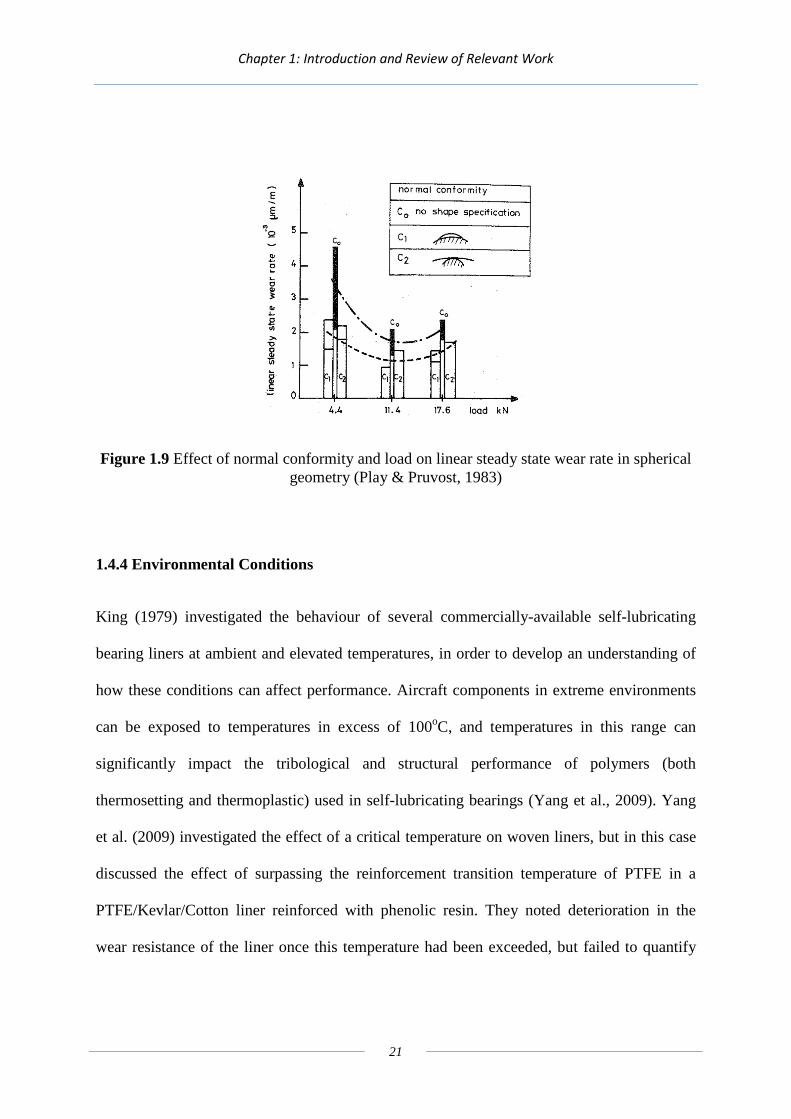
Play & Pruvost (1983) also investigated the effect of conformity on bearing wear rate. They
tested three bearings – one with normal close-tolerance conformity (C0), one with an
increased closed shape (C1) and one with an increased open shape (C2), as shown in Figure
1.9, with the results displayed as bars, with the spread of results shown as blocks at the top of
the bars. Figure 1.9 shows that when the conformity was reduced in either a closed or open
shape, the wear rate was decreased considerably. Play & Pruvost do not offer any explanation
for this feature, other than as an indicator that small changes in bearing geometry can have a
considerable influence on the lifespan of the bearing. They also noted that reduced-
conformity bearings exhibited a significantly increased no-load torque, but they did not
attempt to correlate the two findings.
Chapter 1: Introduction and Review of Relevant Work
21
Figure 1.9 Effect of normal conformity and load on linear steady state wear rate in spherical geometry (Play & Pruvost, 1983)
1.4.4 Environmental Conditions
King (1979) investigated the behaviour of several commercially-available self-lubricating
bearing liners at ambient and elevated temperatures, in order to develop an understanding of
how these conditions can affect performance. Aircraft components in extreme environments
can be exposed to temperatures in excess of 100oC, and temperatures in this range can
significantly impact the tribological and structural performance of polymers (both
thermosetting and thermoplastic) used in self-lubricating bearings (Yang et al., 2009). Yang
et al. (2009) investigated the effect of a critical temperature on woven liners, but in this case
discussed the effect of surpassing the reinforcement transition temperature of PTFE in a
PTFE/Kevlar/Cotton liner reinforced with phenolic resin. They noted deterioration in the
wear resistance of the liner once this temperature had been exceeded, but failed to quantify
Chapter 1: Introduction and Review of Relevant Work
22
the extent of the reduction in wear performance.
King (1979) adopted an early version of the testing apparatus used by Lancaster (1979) to
generate a reciprocating line contact. He showed that an increase in temperature to 100oC
above ambient could increase the wear rate of some materials, particularly those
incorporating reinforcement and other inorganic materials in the weave pattern, by a factor of
10. Evans (1978) noted a similar pattern when testing PTFE composites, and attributed this
effect to the increased temperature hindering the creation of a PTFE transfer layer. Lancaster
(1981) also attributes the temperature-dependent effects to the formation of a transfer layer
being inhibited, and postulates it may be due to the reduction in either cohesive or adhesive
forces at the third-body/wear debris interface at elevated temperatures.
While some materials do show temperature-sensitivity in their steady-state wear rates, King
(1979) found that the “knee” depth of some materials was not dependent on ambient
temperature. King was also not able to extrapolate these results to a prediction of bearing
performance, as he noted that some materials which performed well in his testing conditions
did not perform as well in full-scale bearing tests, and vice-versa. In addition, he noted that
little data were available on full-scale bearing tests, as these are for the most part often
carried out by bearing manufacturers for developed materials and not for experimental
materials which are still in development.
Floquet et al. (1977) identified contact interface temperature as one of the key factors

Chapter 1: Introduction and Review of Relevant Work
23
affecting bearing performance, and created a numerical model to understand the influence of
certain bearing design decisions. They found that the interface temperatures were highest
when the bearing was subjected to a reciprocating motion compared to a uni-directional
rotating motion, and when the bearing liner was attached to the rotating shaft instead of the
static housing (Floquet & Play, 1981).
Humidity is another factor in bearing performance, particularly seen in “bearing torque”,
which is the torque of a bearing under no load. This has been noted to vary for the same
bearing day-to-day at very similar ambient temperatures, and this is often attributed to
variations in humidity (Bell, 2012b). Morgan and Plumbridge (1987) investigated the effect
of humidity on the ultimate tensile strength, indentation recovery and bearing torque of a
woven composite. They used an apparatus housed in sealed humidity cabinets to undertake
tests, so they could vary the humidity of the environment. They noted that the ultimate tensile
strength was reduced by approximately 25% when humidity was increased from 20% to 80%,
and that specimens under lower humidity conditions exhibited more deformation under load
than in higher humidity conditions. This would indicate that the strength of the material is
reduced under high humidity conditions, while its stiffness increases. They rationalised this
discrepancy in that the reinforcement components, which are the greatest factor in the
strength of the material, become weaker when exposed to moisture, whereas the swelling of
the PTFE component under higher humidity leads to a more tightly packed structure, which
increases the overall stiffness. In addition, they noted that bearing torque was approximately
30% higher in bearings at a humidity of 80% than at 20%. Importantly, they noted that the
material took around 20 hours to respond to a change in humidity, meaning it is not affected

Chapter 1: Introduction and Review of Relevant Work
24
by short-term changes in humidity. They discuss the relationship between bearing torque and
humidity proposed by Kuhn, but show that this relationship gives an estimate of bearing
torque that is an order of magnitude too large, and conclude that there are not enough
available data to propose their own relationship. They also conclude that the effect of
temperature variation on bearing torque could be attributed to the associated variation in
humidity due to temperature change.
The effect of humidity on wear rate was investigated by Moreton (1983). In sample tests, he
noted no influence on the wear rates of materials with humidity in the range of 0.1% to 90%
when the tests were loaded under a line contact conditions, however, he noted increases in
wear rate up to 2.5× with some of the same materials in a point contact, while others
maintained their insensitivity. In contrast to Morgan and Plumbridge (1987), he observed no
effect on friction coefficient due to humidity level. He found the materials most affected by
humidity were polyamide, graphite and Aramid. Graphite was particularly susceptible to
increased wear when near 100% humidity occurred and condensation began, leading to an
increase in wear rate of 15×.
Much work has also been undertaken on the effect of contamination of bearings by fluids, as
this is often an unavoidable operating condition (Lancaster, 1982). Bramham et al. (1980)
identified a range of fluids which were detrimental to bearing life, but found no trend for
predicting the effect of an untested fluid based on a known property, such as viscosity. They
also found that some mineral oils gave improved performance. All tests were undertaken

Chapter 1: Introduction and Review of Relevant Work
25
however at one sliding speed and load, therefore the influence of different fluids could very
easily have varied under different operating conditions.
1.5 Tribology of Dry Sliding
The Laboratoire de Méchanique des Contacts (Laboratory of Contact Mechanics) at INSA,
Lyon, carried out a large amount of work on friction and particularly wear of dry sliding
materials. In their paper of 1980, Godet et al. attempt to apply some principles of lubricated
tribology theory to dry sliding, particularly with regard to the formation and transport of third
body debris. In particular they highlight the enormity of the effect that third body debris can
have on the wear rate of a dry sliding system, dependent on whether it is entrained within or
ejected from the contact area.
The principle of wear proposed is that a third body is formed from wear debris within the
contact through some wear mechanism, i.e. adhesion or abrasion, which is then progressively
removed from the contact area (Play, 1985). The volume of wear is therefore the volume of
debris lying outside the contact area. Depending on the material, the debris can also form a
“third-body film” or transfer layer. The thickness of this transfer layer depends on the amount
of wear debris generated and the ratio of the contact area between a sample and the
counterface and the length of the counterface. This seems fairly obvious, as if it is assumed
all wear debris becomes a transfer layer of uniform thickness, the thickness of the layer will
be:

Chapter 1: Introduction and Review of Relevant Work
26
wear volume (m3) / total contact area over a cycle (m2) = thickness of transfer layer (m)
Play (1985) noted that the transfer layer is not uniform, and tends to be thicker towards the
centre of the contact. This is explained by Godet et al. (1980), who discussed how wear
debris can only be ejected from the edges of a contact, therefore debris entrained in the centre
of the contact cannot easily be removed, as in “wet” lubrication theory of un-sealed journal
bearings. Play (1985) also noted that the coefficient of friction and wear rate is considerably
lower in oscillating motion than in uni-directional sliding, a finding supported by Lancaster et
al. (1982). Play (1985) described contacts in terms of a Mutual Overlap Coefficient (MOC),
defined as the ratio of the contact area of the sample to the total contact area of the
counterface traversed by the sample. Play tested the effect of MOC using chalk pins on a
glass counterface. When the vertical displacement of a pin is compared with time, a curve
very similar to that observed by King (1979) is seen, with three distinct phases. The running
in period is, however, much shorter as a proportion of overall test duration. They noted that
wear rate is reduced when this MOC ratio is high (a short stroke length) but the friction
coefficient is increased. However, it is important to note that both these values are taken from
the final “running out” part of the wear curve, and not from the steady-state period. These
effects cannot therefore be directly compared with the literature on bearing liners, where wear
rate and friction coefficient are typically taken during the “steady-state” phase of their wear
curve.
The development of a third body transfer layer is attributed to lower wear rates, and this is
described as a “self-protective” feature of dry sliding materials (Play & Godet, 1977). Play

Chapter 1: Introduction and Review of Relevant Work
27
and Godet (1977) described this self-protective feature as dependent on the length of the
contact normal to the sliding direction, and independent of the width. They proposed a model
with two contact zones, as seen in Figure 1.10 taken from the paper. In the “frontal area”
(denoted A1 on Figure 1.10), wear debris is formed by interaction with asperities of the
counterface, and the debris fills the gaps between the asperities. Excess debris then forms a
third body film on top of the counterface, and the friction and wear of the “eye” (denoted A2
on Figure 1.10) is governed by the interaction between the sliding material and the third body
layer, the wear of which can be described as a “polishing” effect and significantly lower than
that encountered by the first zone. The third body film in the second zone will “lift” the front
zone away from the contact slightly, reducing the load carried by this high wear region, and
therefore the overall wear rate of the contact.
Figure 1.10 Two-zone contact (Play & Godet, 1977)
Direction of travel
d
A1
A2

Chapter 1: Introduction and Review of Relevant Work
28
In reciprocating motion, if the length of the specimen is greater than 2 × d from Figure 1.10,
the centre of the specimen will only ever interact with a transfer layer, which explains the
observation of Play (1985) that transfer films on both the specimen and the counterface are
significantly thicker at the centre of the contact area.
Godet & Play investigated the effect of fibre alignment with respect to sliding direction in an
epoxy-filled carbon fibre composite. They noted that if the fibres were aligned normal to the
sliding direction, the coefficient of friction was reduced by 25% compared to the case in
which fibres were aligned parallel to the sliding direction, as shown in Table 1.1. If the fibres
are oriented at 45 degrees to the sliding direction however, the coefficient of friction is only
increased by 4% compared to the case in which the fibres are parallel to the sliding direction.

Chapter 1: Introduction and Review of Relevant Work
29
Table 1.1 Coefficient of friction dependent on fibre orientation (Godet & Play, 1975)
Fibre Alignment Coefficient of friction
0.16
0.12
0.19
0.125
Kennedy et al. (1975) investigated the factors affecting the wear of polyethylene against a
steel counterface. They found that wear rate decreases when moving from a very rough
surface to a smoother surface, but found a point at which increasing the smoothness of the
surface further increases the wear rate. In the case of polyethylene on steel, they found this
roughness to be 0.1 µm Ra. They also found that the coefficient of friction is decreased with
rougher surfaces. They rationalised this as due to the combined effect of adhesion and third
body thickness. They stated that the main frictional mechanism between polyethylene and
steel is adhesion, which is significantly reduced by the formation of a third body film. As a
rougher surface allows the third body film to be generated and held between the asperities,
this reduces the effect of adhesion and therefore the coefficient of friction. They did not

Chapter 1: Introduction and Review of Relevant Work
30
however extend this hypothesis to explain the increase in wear rate against very smooth
surfaces, though as the trends are the same when surface roughness is compared to both
coefficient of friction and wear rate, such an extension would seem logical.
The work of Bramham et al. (1980) identified a range of fluids which were detrimental to
overall bearing life, and showed that their effect was increased when a constant supply of the
fluid was introduced. They presented one possible explanation for this as the fluid inhibiting
the creation of a transfer layer, or continuously removing the one already formed (Lancaster,
1972). This suggestion is supported by micrography of the surfaces compared to the same
materials examined in dry conditions (Evans, 1978). This further underlines the importance
of the creation and maintenance of a transfer layer in the performance of self-lubricating
materials. Moreton (1983) uses the effects of fluids inhibiting the creation of transfer layers
to explain the huge detriment to performance experienced with some materials when
operating in near 100% humidity, where water condensation at or near the contact zone is
possible.
1.6 Computer Modelling of Self-Lubricating Bearings
Computerised modelling is a relatively new technology in the field of self-lubricating
bearings, and has only recently started to be applied. Metal-on-metal journal bearings are
relatively simple, and can often be modelled using conventional continuum mechanics
principles. The introduction of a composite self-lubricating liner, with non-homogenous
material properties, increases the complexity of the modelling problem significantly.

Chapter 1: Introduction and Review of Relevant Work
31
Fortunately, Finite Element Modelling (FEM) is an accessible method of computationally
modelling structures, with many commercial software packages available to carry out
simulations. Modelling is possible on the scale of the fabric itself using finite element
techniques (Parsons et al., 2010), but it is currently considered unrealistic to model the
bearing liner on the scale of the bearing with the necessary degree of detail.
Cao et al. (2010) investigate the effect of including heat generated due to friction on the
contact stresses in a spherical self-lubricating bearing, with a PTFE-based composite fabric
liner. They compared the results of theoretical temperature analysis and FEM temperature
analysis, and found good agreement between both techniques and experimental data. They
found that the peak contact stress in the bearing was increased by approximately 30% due to
the inclusion of the effect of expansion due to frictional heating.
Liu and Shen (2010) propose a mathematical method of combining the elastic properties of
yarns in a composite fabric containing PTFE and C-50 carbon. They obtained very good
agreement between the elastic modulus of the fabric found by computational and
experimental methods (0.63% difference) and good agreement for the Poisson’s ratio
(12.74% difference).
Some studies have considered the liner as a bulk material, with elastic (Li et al., 2008) or
hyperelastic (Yang et al., 2010) properties. These properties are usually selected after
matching to the experimentally derived stress-strain curve. Li et al. (2008) modelled a self-
Chapter 1: Introduction and Review of Relevant Work
32
lubricating spherical plain bearing with a fabric bearing liner containing Aramid and PTFE
with a synthetic resin. This liner was considered as a laminate, which contains the correct
proportions of the materials but neglects the weaving pattern. The bearing was modelled as
three parts – the inner ring, the bearing liner and the outer ring. The stiffness and Poisson’s
ratio of the liner was calculated by combining the stiffness and Poisson’s ratio of the Aramid
and resin, as the PTFE was ignored due to its low volume fraction. These properties were
then applied to a bulk material representing the liner. This method produced good agreement
between experimental and FEM results (<10% variation) for the displacement of an inner
ring into the liner material under load.
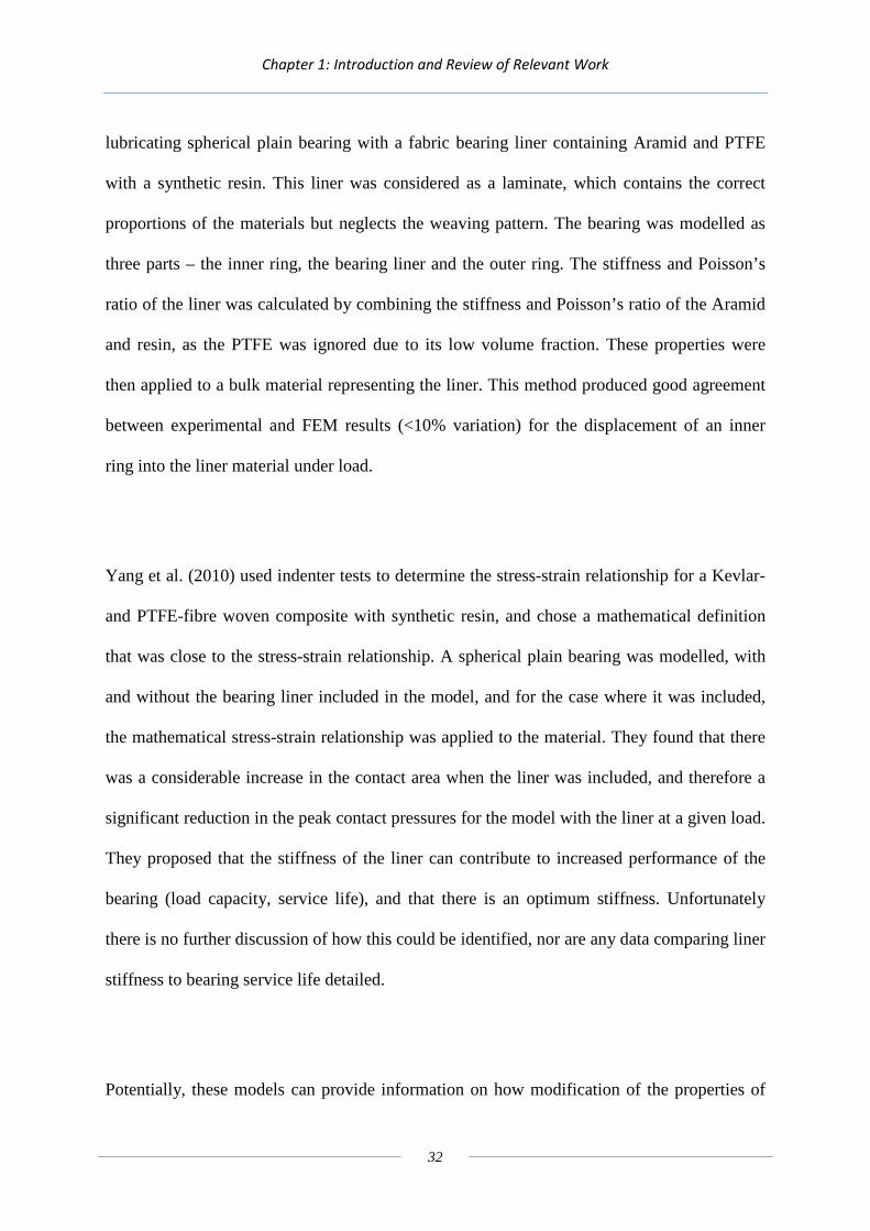
Yang et al. (2010) used indenter tests to determine the stress-strain relationship for a Kevlar-
and PTFE-fibre woven composite with synthetic resin, and chose a mathematical definition
that was close to the stress-strain relationship. A spherical plain bearing was modelled, with
and without the bearing liner included in the model, and for the case where it was included,
the mathematical stress-strain relationship was applied to the material. They found that there
was a considerable increase in the contact area when the liner was included, and therefore a
significant reduction in the peak contact pressures for the model with the liner at a given load.
They proposed that the stiffness of the liner can contribute to increased performance of the
bearing (load capacity, service life), and that there is an optimum stiffness. Unfortunately
there is no further discussion of how this could be identified, nor are any data comparing liner
stiffness to bearing service life detailed.
Potentially, these models can provide information on how modification of the properties of

Chapter 1: Introduction and Review of Relevant Work
33
the fibres and resin affect the stiffness of the liner, but they cannot give any indication of the
effect on friction and wear of the liner. Other modelling methods have approached the
problem of predicting friction and wear. Bortoleto et al. (2012) use a custom script in a
commercially available finite element software to describe the removal of material due to
wear in a dry sliding pin-on-disc test incorporating an Archard wear law formulation. They
calculate friction in the model by calculating the tangential force needed to move the pin and
dividing it by the normal load. However, it is not entirely clear what governs the force needed
to move the pin, as they do not specify a coefficient of friction between the pin and the disk.
In any case their results using this method lead to predicted coefficients of friction between
40% and 70% lower than those observed in experiments. Their results for wear show a
similar magnitude of error, but consistently over-estimate the wear depth.
The discrete element modelling approach has an advantage over finite element modelling in
that wear is very easy to simulate (Richard et al., 2007). In the discrete element method, a
material volume is represented by a cluster of spheres, for which interactions are specified.
The method models not only wear, but allows the movement of third bodies to be tracked
(Fillet et al., 2005). The method also enables thermal effects to be studied in a similar manner
to the finite element method (Richard et al., 2008). These theoretical methods do not appear
to have been verified experimentally, however, and there are concerns regarding the
assumptions made on the size and distribution of wear particles, which are partly governed by
user inputs, which can have a major effect on the predictions of the model (Fillot et al.,
2005).

Chapter 1: Introduction and Review of Relevant Work
34
1.7 Future Development of Bearing Liners
As self-lubricated bearing tribology has progressed, attempts have been made at improving
the performance of bearing liners by using new materials. Li &Ran (2010) found carbon-fibre
reinforcement to give improved wear performance over other reinforcement materials in non-
woven composites. Considerable work has also been undertaken in evaluating the
performance of different resins in woven materials. Verma et al. (1996), for example, found
improved performance of a phenolic resin in a woven composite when the resin was
chemically modified with Poly Vinyl Butryal (PVB). The specific wear rate (mm3N-1m-1) was
reduced by between 20% and 80% in comparisons with non-modified phenolic resin, with a
corresponding reduction in coefficient of friction of between 10% and 50%, dependent on
sliding velocity. The modified resin possesses around 5% higher tensile strength and flexural
modulus, with 7% reduced flexural strength. Importantly, the modified resin has an 80%
higher tensile modulus, and 75% higher Charpy impact energy (kJ m-2). The authors
concluded that the reduction in wear rate was due to the increased ductility of the resin. There
was also a reduction in bulk surface temperature rise of between 20% and 50% observed
through use of the modified phenolic resin, which is a considerable factor in the context of
friction and wear of thermosetting materials (Yang et al., 2009). The effect of temperature on
the pattern of friction and wear observed is discussed. In particular the authors identify a
critical temperature above which “charring” of the resin is observed, the effect of which is to
significantly increase the friction coefficient and wear rate. The theoretically ideal
temperature is one which is high enough to reduce the friction coefficient and wear rate by
increasing the ductility of the resin, but not so high as to cause “charring” and bring about a
reduction in the material properties of the resin.

Chapter 1: Introduction and Review of Relevant Work
35
Investigations into the performance of alternative resin materials are of particular commercial
importance at the present time, as the many phenolic resin systems utilise formaldehyde, the
use of which is coming under increasingly strict regulations (Wagner, 2010). It is therefore
timely to develop new methods of tribologically simulating self-lubricated bearings which
can be used as screening tools for the rapid evaluation of candidate material combinations.
1.8 Aims & Objectives
The project aims to fulfil the following objectives:
• To produce a finite element model of a composite dry bearing liner, providing a
representation of all constituent materials.
• To use this finite element model to inform a model of the variation in friction
coefficient over the wear life of the bearing liner, which will take into account the
changing proportion of the constituent materials in contact with the counterface.
• To verify this friction model against experimental data obtained from a bespoke flat-
on-flat sample wear test bench.
• To model the useful wear life of a complete “dry” spherical plain bearing containing
the bearing liner, and verify predicted wear against results from full-scale bearing
tests undertaken outside of the project. The approach will apply lubricated journal
bearing theory to a “dry” spherical plain bearing.
There are two aspects to the project which are novel – firstly, the modelling of the friction

Chapter 1: Introduction and Review of Relevant Work
36
coefficient of a multi-material tribological contact and its variation throughout the wear life
of a composite material. Secondly, the modelling of the wear life of a complete “dry”
spherical plain bearing using lubricated journal bearing theory.

Chapter 2: Modelling the Weave
37
2. Modelling the Weave
2.1 Objectives
Composite bearing liners have been available since the late 1960s (Lancaster, 1982). Physical
testing of new bearing liners is both costly and time-intensive, therefore methods of screening
potential new composites are urgently sought.
There are three key performance characteristics of bearings:
• Load-bearing capacity – dependent on the stiffness and ultimate tensile strength of the
component materials.
• Efficiency – dependent on the overall friction coefficient of the bearing.
• Lifespan – dependent on the wear rate and any failure modes.
There are additional characteristics of bearings required for certain applications, such as
resistance to corrosion and contaminants, and the ability to operate at extreme temperatures.
An improved bearing liner would show improvements in one or more of the key performance
characteristics. In order to model any of these parameters for a new fabric before the
prototyping phase, some method of simulating the fabric’s response under realistic conditions
is required.

Chapter 2: Modelling the Weave
38
It was decided that a finite element analysis (FEA) model should be developed to simulate a
composite bearing liner, using the commercial finite element software DSS Abaqus. This
would allow estimation of the three key bearing characteristics in the following way:
• Load-bearing capacity – a finite element model of the constituent materials of a
bearing liner would allow an overall stiffness to be calculated.
• Efficiency – a friction model would use the variation in contact pressure and the
proportion of materials in contact over the wear-life of the liner to estimate the
friction coefficient corresponding to different amounts of wear.
• Lifespan – the wear rate of a composite material is affected by the variation in
stiffness at different amounts of wear.
To evaluate the effectiveness of models of this sort, it would be necessary to test them in
terms of a pre-existing material, so that information on the three key performance
characteristics of the bearing liner could be obtained. The end goal of these models (beyond
the scope of the project) is to develop a method of screening potentially new composite
fabrics.

Chapter 2: Modelling the Weave
39
2.2 Weave Visualisation
It was anticipated that the simplest finite element model of the test bearing liner is that of a
“unit cell” – the smallest repeating geometry – subject to boundary conditions to make it
behave as part of a much larger sheet of the material. In order to preserve commercial
confidentiality and intellectual property, only a portion of the unit cell is illustrated in this
version of the thesis.
While the specification of the fabric was obtained from manufacturing specifications, the
fabric was still difficult to visualise due to its complex structure. Texgen is software
developed by the University of Nottingham to “model the geometry of textile structures”
(Texgen, 2013). This software was used to develop a visualisation of the test fabric in 3D,
shown in Figure 2.1.
Figure 2.1 Visualisation of part of the test fabric weave, using Texgen

Chapter 2: Modelling the Weave
40
2.3 Finite Element Model
2.3.1 Unit Cell Geometry
Finite element models were first developed in two dimensions, to evaluate methods for
specifying a composite material structure. DSS Abaqus finite element models contain “parts”
– individual components which are either free to act independently or are constrained in some
way to simulate part of a larger assembly. Parts generally have a single material property for
the whole part even if the part is made of a composite material, in which case non-
homogenous material properties can be specified. In order to model the test composite unit
cell as one part on the micro scale, different material properties had to be specified for
different sections of the part. It would have been possible to create the “unit cell” from
multiple parts representing the yarns and the resin and specifying their interactions, but it was
anticipated that this would create a complex, inflexible model. A method was necessary to
specify the composite material structure using only one part, but containing multiple material
assignments.
An initial attempt to create multiple material definitions was performed element-by-element.
Due to the regular numbering structure for elements in regular meshes in DSS Abaqus,
elements could have material properties specified by creating sets of element numbers,
identifiable from their predicable pattern. Figure 2.6 shows a single “part” made up of two
alternating material definitions, specified by element number. Figure 2.2 also shows an
illustration of how the predictable pattern of element numbering allows sets of element
numbers to be built to create such a “part”. A weave-like structure created using this method

Chapter 2: Modelling the Weave
41
is illustrated in section Figure 2.3.
Figure 2.2 A single “part” made up of two materials, with an area magnified showing an example of the element numbering system
In this example, 2 sets of element numbers would be created – 1,3,5,7,9 for Material 2 and 2,4,6,8 for Material 1.
Figure 2.3 A weave-like pattern specified by element number
Material 1
Material 2
1 2 3
4 5 6
7 8 9

Chapter 2: Modelling the Weave
42
This method was found to have two limitations which prevented it from being extended to 3D
models. Firstly, element numbering is mesh-dependent. Changing the mesh density changes
the size of elements, therefore a given area would have different numbers of elements. Using
this method new sets of element numbers had to be created every time a different mesh was
specified. Secondly, when less regular meshes were used, as required when a mixture of
element types were used, the mesh numbering pattern became less predictable and it was very
difficult to build the necessary element number sets.
A more flexible method of specifying sections and materials was developed which used a
bespoke script with a series of commands, written in the Python programming language. The
make-up of the script is described in detail in Chapter 3. This script creates a 3D Finite
Element model of the weave with a structure representative of the test composite fabric.
Figure 2.4 shows the “unit cell”, made up of PTFE yarns and reinforcement yarns in a resin
matrix. Figure 2.5 is the same “unit cell” but with the resin hidden, to show the weave
structure, which is compared with the weave structure visualised using Texgen (Figure 2.1).

Chapter 2: Modelling the Weave
43
Figure 2.4 Part of a “unit cell” of test composite fabric, made up of PTFE and reinforcement yarns in a resin matrix
Figure 2.5 Part of a “unit cell” of test composite fabric, as Figure 2.4 but with resin hidden to show the weave structure
The geometry of the unit cell is designed around the concept of dividing the test composite
into three “layers” – a reinforcement warp layer; a layer of resin to allow the weft to pass
between the warp yarns; and a PTFE warp layer. In application, the PTFE warp layer would
be the layer initially in contact with the moving part. Figure 2.6 shows this division into
layers on the “unit cell”, and Figure 2.7 shows a cross-section through the weft of the test
fabric, alongside the same diagram but with only 1 warp thread shown.

Chapter 2: Modelling the Weave
44
Figure 2.6 Part of unit cell showing three “Layers” of Finite Element Model
Figure 2.7 Part of a cross-section in the warp direction showing only one weft thread

Chapter 2: Modelling the Weave
45
The cross-sectional diagram in Figure 2.7 implies the need for five “layers” as shown in
Figure 2.8 – a layer for weft threads passing over the reinforcement warp (1); a layer for the
reinforcement warp (2); a layer between the reinforcement warp and PTFE warp (3); a layer
for the PTFE warp (4); and a layer for weft threads passing underneath the PTFE warp (5).
Figure 2.8 Part of a cross-section through the warp, showing five layers - a layer for weft threads passing over the reinforcement warp (1); a layer for the reinforcement warp (2); a
layer between the reinforcement warp and PTFE warp (3); a layer for the PTFE warp (4); and a layer for weft threads passing underneath the PTFE warp (5).
It was seen from tomography of the test composite fabric that where a weft thread passes over
a warp thread, it displaces the warp thread into the inter-warp layer, hence there is no need
for layers 1 and 5. This is highlighted in Figure 2.9, featuring a magnified view of a weft
thread being pulled into the inter-weft layer.

Chapter 2: Modelling the Weave
46
Figure 2.9 Tomography showing cross-section through the weft (top), with warp thread highlighted in blue, along with reinforcement weft thread which has been displaced into the
inter-weft layer in red
Figure 2.10 shows the three-layer approach based on Figure 2.9, showing the reinforcement
warp layer (1); the inter-warp layer (2); and PTFE warp layer (3). Figure 2.11 shows this
same structure in the finite element “unit cell”.
Figure 2.10 Part of a cross-section through the warp, showing 3 layers - the reinforcement warp layer (1); the inter-warp layer (2); and PTFE warp layer (3).
Figure 2.11 Part of a cross-section through the warp of the finite element “unit cell” showing only one weft thread, with displaced warp threads and layer divisions highlighted
1
2
3

Chapter 2: Modelling the Weave
47
From examination of the tomography of the test composite fabric, it was also found that the
inter-warp layer was much thinner than the two warp layers. Figure 2.11, for example, shows
the dimensions of these layers superimposed on the test tomography, with the yellow
measurement lines in the figure taken as average heights; for example the top line represents
the average height of the top surface across a sample. The figure shows the reinforcement
warp and PTFE warp layers are thicker than the inter-warp layer. Figure 2.12 shows the FEA
model with three equal layers and in the modified form with a reduced inter-warp layer
thickness.
Figure 2.11 Tomography showing cross-section through the weft of the test composite fabric
Figure 2.12 Part of a cross-section through the weft of test composite “unit cell”, with three equal layers (top) and reduced inter-weft layer thickness (bottom)

Chapter 2: Modelling the Weave
48
The full unit cell was then assembled between two rigid planes on the top and bottom. The
top plane has a uniform pressure over its top surface of 1 N/mm2 and is only allowed to
displace in the y-direction (perpendicular to the plane). The bottom plane is constrained in all
directions to prevent any movement. This set of constraints and loading represents
compression of the composite fabric between two flat platens, shown in Figure 2.13. Contact
was therefore simulated between the two rigid planes and the unit cell. The simulation gives a
contact pressure distribution on the bottom (contact face) surface of the unit cell, which will
vary based on the stiffness of the materials in contact and the materials directly above them.
The results of these simulations are discussed in Chapter 5.
Figure 2.13 Part of “Unit cell” assembled between two rigid planes (left) with “unit cell” hidden (right) to show only rigid planes

Chapter 2: Modelling the Weave
49
2.3.2 Contact Settings and Element Selection
DSS Abaqus offers a wide range of options for specifying contact in a model, together with a
range of element types. Not all possible options for contact and element selection are
discussed in this section, as full information can be found in the DSS Abaqus User Manuals.
The contact conditions for the finite element model are relatively simple compared to some
more complex models DSS Abaqus is capable of simulating, therefore the settings used are
close to the recommended default settings. This section discusses only the contact controls
which were changed from the default settings, or where there is no default setting. The
selection of elements is also discussed, as certain element types are unsuitable for contact
modelling.
Contact between two bodies in DSS Abaqus is defined by a master and slave surface, with
the condition that slave nodes cannot penetrate a master surface, but master nodes can
penetrate a slave surface. It is recommended that the master surface is defined as the more
coarsely meshed surface. In this model, the two rigid planes were selected as master surfaces,
and the unit cell faces were defined as the slave surfaces.
DSS Abaqus offers two options for contact discretization – node-to-surface and surface-to-
surface, and two options for contact formulation – small-sliding and finite sliding. Except in
borderline cases where convergence is difficult, DSS Abaqus recommends the use of surface-
to-surface contact discretization for maximum accuracy. Figure 2.14 shows an excerpt from
the DSS Abaqus manual, comparing the two contact discretization methods and showing the

Chapter 2: Modelling the Weave
50
surface-to-surface method to be at least an order of magnitude more accurate.
Figure 2.14 Contact discretization methods and their accuracy (DSS Abaqus, 2012)
There are two options available for contact formulation – small-sliding and finite-sliding.
Small sliding is a contact approximation method designed to reduce the solution computing
time, but it can produce results which are not physically meaningful if some sliding is
occurring at the interface. The finite sliding method is, by comparison, more robust, and

Chapter 2: Modelling the Weave
51
highly recommended for all contact problems (DSS Abaqus, 2012). In this model, the finite
sliding formulation is used in both contact interfaces between the “unit cell” and the rigid
planes.
DSS Abaqus offers three possible 3D element shapes – tetrahedral (“tet”), hexahedrons
(“brick”) and pentahedral (“wedge”), shown in Figure 2.15.
Figure 2.15 3D Element types (left to right) – tet, brick and wedge (Moreno, 2012)
Each element type has two main derivatives – first-order and second-order. First order
elements have a node at each vertex of the element; therefore in the case of a six-sided brick
element there are eight nodes. Second-order elements also include a node at the midpoint of
each side, so in the case of a six-sided brick element there are twenty nodes, as illustrated in
Figure 2.16.

Chapter 2: Modelling the Weave
52
Figure 2.16 First-order and Second-order brick elements showing the number and position of nodes
Second order elements are generally more accurate for modelling stresses, but their use incurs
a computational cost penalty. For the application of a contact pressure to a brick element, in
the case of the first-order element, the pressure is equally divided amongst the 4 nodes in
contact. In the case of the second-order element however, the pressure is not equally
distributed amongst the eight nodes in contact, as shown in Figure 2.17.
Figure 2.17 Equivalent nodal loads produced by a constant pressure on the second-order element face in a contact simulation
Chapter 2: Modelling the Weave
53
As the output of this finite element model would need to be processed and understood outside
of the DSS Abaqus Visualisation program, first-order elements were chosen so that pressures
values output by node would be more representative of the contact stresses.
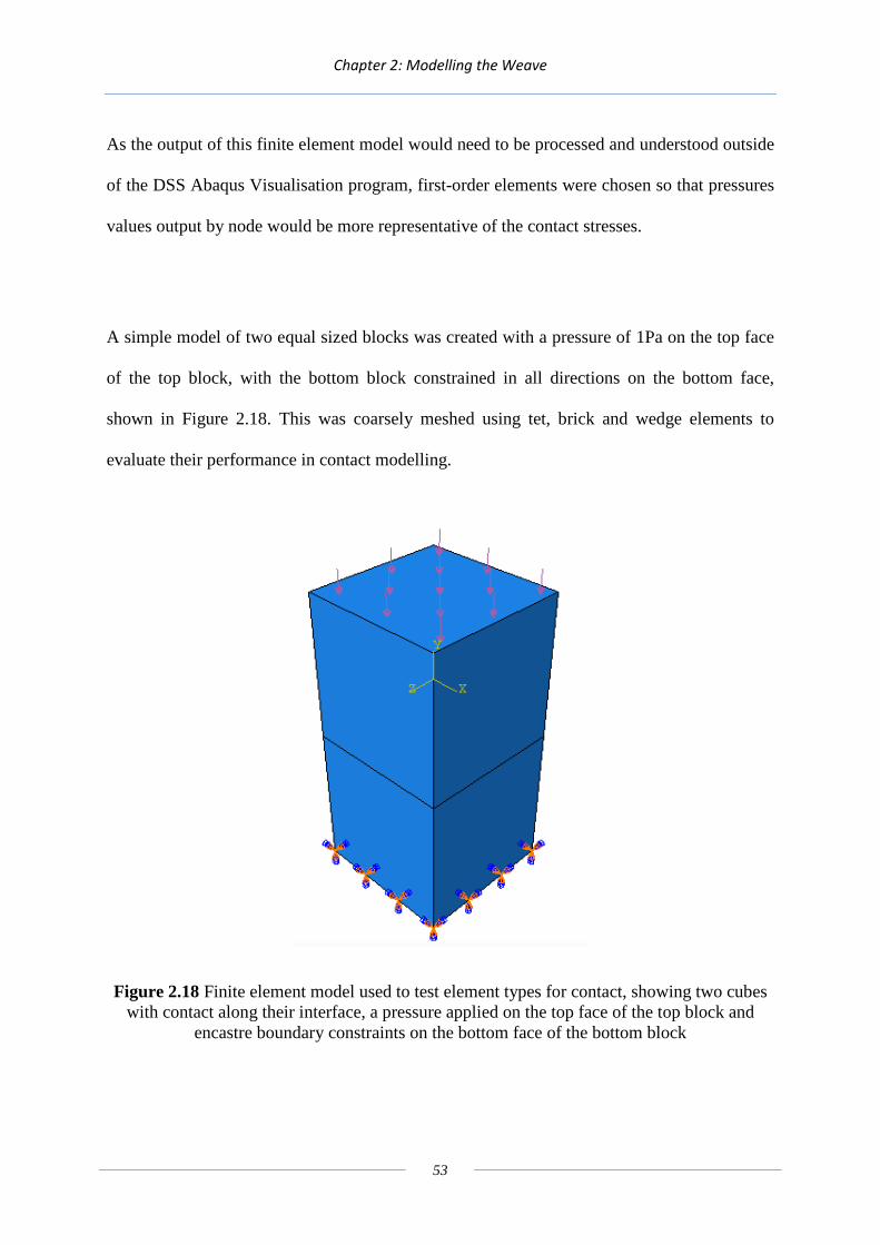
A simple model of two equal sized blocks was created with a pressure of 1Pa on the top face
of the top block, with the bottom block constrained in all directions on the bottom face,
shown in Figure 2.18. This was coarsely meshed using tet, brick and wedge elements to
evaluate their performance in contact modelling.
Figure 2.18 Finite element model used to test element types for contact, showing two cubes with contact along their interface, a pressure applied on the top face of the top block and
encastre boundary constraints on the bottom face of the bottom block

Chapter 2: Modelling the Weave
54
The results of the analysis are shown in Figure 2.19. Both brick and wedge elements
produced a uniform pressure distribution as expected, whereas the tet elements produced a
non-uniform pressure distribution, with variations of up to 0.6% from the mean pressure
value. This small deviation in contact pressure, along with possible problems with shear
locking in non-linear analyses such as contact (Puso, 2006), led to tet elements being
disregarded as suitable elements to mesh the unit cell.

Chapter 2: Modelling the Weave
55
Figure 2.19 Pressure distributions for brick and wedge elements (top and middle) and tet elements (bottom) for the same finite element model

Chapter 2: Modelling the Weave
56
First-order elements were used throughout the unit cell. Quadratic elements could not be used
in areas away from the contact without significantly increasing the complexity of the model
due to the need for complex tie interfaces between first- and second-order elements. Wedge
elements were used in the weaving sections of the model, as these are accurate in contact
calculations, and are also able to fit into the triangular sections of the model without extreme
element distortion. Brick elements were used to represent the weft thread areas. Figure 2.20
shows a cross-section through the weft of the finite element model, with a reinforcement
warp yarn shown, and no mesh. Figure 2.21 shows the same model meshed only using brick
elements, alongside the same mesh with elements highlighted in yellow where there is
enough distortion to potentially effect the accuracy of the results. Figure 2.22 shows the mesh
that was used in the unit cell, which consists of brick elements for the weft thread areas
(highlighted in orange) and wedge elements used for all other areas (highlighted in blue).
Wedge elements were used in the areas with triangular sections as their native shape lends
itself to use in triangular sections.

Chapter 2: Modelling the Weave
57
Figure 2.20 Part of a cross-section through the warp showing reinforcement weft thread without mesh
Figure 2.21 Part of a cross-section through the warp showing reinforcement weft thread meshed using brick elements (left) alongside the same mesh with excessively distorted
elements highlighted in yellow (right)
“Brick” Elements “Wedge” elements
Figure 2.22 Part of a cross-section through the warp showing reinforcement weft thread meshed using wedge and brick elements (left), with brick elements highlighted in orange and
wedge elements highlighted in blue (right)

Chapter 2: Modelling the Weave
58
2.3.3 Harmonic Boundary Conditions
Once a representative unit cell of the test composite fabric had been created, boundary
conditions had to be specified which would make the unit cell behave as if part of a much
larger overall liner, as illustrated in Figure 2.23.
Figure 2.23 “Unit cell” displayed as part of a larger liner
Figure 2.24 shows a finite element model of a block with a repeating pattern of material
assignment compressed between two platens. The bottom platen is fixed, and the top platen is
constrained to move only in the y-direction. The top platen is displaced to give a compressive
strain of 0.9. The block has a height of 1, and a length of 20, with each section possessing the
dimensions of 1×1, each with 10,000 elements. The block has a repeating pattern of material
assignment, with both materials having the same stiffness but with Material 1 having a
Poisson’s ratio of 0.3 and Material 2 having a Poisson’s ratio of 0. This means that sections
with the properties of Material 1 will have edge effects, and those with Material 2 will not.
Figure 2.25 shows the stress contours produced by this simulation, with a close-up of a
repeating unit cell at the centre of the part, away from any edge effects.

Chapter 2: Modelling the Weave
59
Figure 2.24 Model of block with repeating pattern of material assignment, Material 1 in green and Material 2 in cream, compressed between two platens in red
Figure 2.25 Results of analysis of model in Figure 2.29 (top) with a close-up of central repeating block (bottom)
Figure 2.26 shows a model of a block with only two sections, which is the repeating unit cell
of the previous model. This model is given the same compressive strain as the previous
model but no additional constraints, and the results are shown in Figure 2.27, which are
significantly different to those seen in Figure 2.25. This means that without additional
constraints this model is not representative of the behaviour of a unit cell at the centre of the
model.
X
Y

Chapter 2: Modelling the Weave
60
Figure 2.26 Unit cell with two materials compressed between two platens in red
Figure 2.27 Results of analysis of model in Figure 2.31
Figure 2.28 shows the results obtained using the same model, but with boundary conditions
imposed on the far left and right hand edges of the unit cell to stop their displacement in the
x-direction. This is again different to the results seen in Figure 2.25, and therefore not
representative.

Chapter 2: Modelling the Weave
61
Figure 2.28 Results of analysis of model in Figure 2.26 but with x-direction constraint boundary conditions applied to left and right hand side of the block
The model was analysed again, however this time the constraints on the left and right hand
sides were changed to harmonic boundary conditions. Harmonic boundary conditions
constrain opposite sides of the unit cell to have equal displacement. This was achieved by
using DSS Abaqus’s “tie” function to keep corresponding points on opposite sides of the
block at a constant separation, and remove “edge effects”. This works by (in this case)
keeping points with the same height but on opposite sides of the block at the same separation
in the x-direction or z-direction. Figure 2.29 shows a schematic representation of this type of
constraint.

Chapter 2: Modelling the Weave
62
Figure 2.29 Loading of a block without harmonic boundary constraints, showing Poisson “edge effects” (top) and the same model with harmonic boundary constraints, which removes
Poisson “edge effects” (bottom)
Figure 2.30 Results of analysis of model in Figure 2.26 but with harmonic boundary conditions applied to left and right hand side of the block
Load
Load

Chapter 2: Modelling the Weave
63
Figure 2.30 shows the results of this simulation, which are now very similar to those seen in
the larger model in Figure 2.25. Figure 2.31 shows the results of the two simulations with the
scale adjusted to increase the detail in the stress contours in the section. The results are very
similar. However, there are slight differences in the contours, for example at the top left hand
and bottom left hand corners of the unit cell model. The unit cell block however reduced the
number of elements in the model by a factor of ten. While it may be possible for the first,
larger model to be reduced in size while still isolating the repeating cell at the centre from
edge effects, the necessity to have multiple unit cells would mean that a model with harmonic
boundary conditions reduced the number of elements by at least a factor of three. Such a
reduction represents enormous savings in analysis time, as the relationship between the
number of elements and the time taken to perform an analysis is not necessarily linear.

Chapter 2: Modelling the Weave
64
Figure 2.31 Results of analysis of model as Figure 2.35 (top) and Figure 2.30 (bottom) with scale adjusted to increase detail of contours

Chapter 2: Modelling the Weave
65
2.4 Assumptions and Limitations
The following assumptions and limitations apply to the unit cell model, each of which are
discussed in this section:
• All threads in the warp direction and all threads in the weft direction have the same
cross-section, though there can be a difference between warp and weft threads, and
the cross-section of all warp and weft threads is rectangular.
• The weft threads are not of constant thickness when passing through the inter-warp
layer.
• There is a smooth, connected weave pattern in the cross-section through the warp, but
not in the weft cross-section.
2.4.1 Thread Cross-Sections
In the finite element model all threads have a rectangular cross-section. This allows much
simpler meshes to be used than if the threads were of circular or elliptical cross-section. The
threads in the finite element model represent bundles of hundreds of individual fibres, a level
of detail which would have been unrealistic to model on the scale of the unit cell. To account
for the fact that the PTFE and reinforcement threads are not of the same dimensions, the
actual total cross-sectional area of all the fibres in the threads was calculated from
manufacturing specifications of the yarns, allowing for the proportion of resin and
reinforcement/PTFE in the unit cell cross-sectional area and the equivalent stiffness for the
unit cell thread. The weight of threads are measured in “denier”, a unit of measurement of the
linear mass density of yarns, defined as the mass in grams of 9,000 m of the thread. The

Chapter 2: Modelling the Weave
66
origin of this traditional unit of measurement is from weaving, where one strand of silk has a
mass of approximately 1 gram per 9,000 metres (Brossard, 1997). From the linear mass
density of the fibres, and the density of the material, the total cross-sectional area of all
filaments in a yarn may be calculated.
The yarns are made up of many filaments, which will have small gaps between them. Denier
is a more useful way of calculating the total cross-section of all the filaments making up the
yarn than physically measuring it, as it is not affected by how tightly the fibres are wound and
how much space is left between fibres in a single yarn. The total cross-section of all fibres in
a yarn is calculated by dividing the linear mass density of the yarns (denier) by 9000, to give
the mass in grams per metre of thread, then dividing by the density of the material, to give the
total cross-sectional area of all threads.
By dividing the total cross-sectional area of the yarns of each material by the cross-sectional
area of the threads in the unit cell, the percentage of the area of the thread made up by the
yarn material can be calculated. The remaining portion of the “unit cell” thread is assumed to
be made up of resin, the simplification being made that there are no air gaps in the test
composite fabric. The stiffnesses of the two materials are combined in these proportions to
give the representative stiffnesses of the reinforcement and PTFE threads which are found to
be in the ration of 70:1.

Chapter 2: Modelling the Weave
67
2.4.2 Variation in Thread Thickness
The model was originally designed with all three layers having the same thickness, which
allowed the cross section of weft threads to remain constant as they passed through the inter-
warp layer. Upon examination of X-ray tomography images it was seen that this inter-weft
layer was in fact much smaller than expected, and the inter-warp layer was therefore reduced
in the finite element model. This was not viewed as having a detrimental effect on predicted
response, as the inter-warp layer is predominantly resin, therefore reducing its size brings the
proportional amount of resin in the model closer to that seen in the finished liner.
2.4.3 Weave Pattern in Warp vs. Weft Direction
Creating a 2D weave pattern was a relatively simple task compared to being able to create a
3D weave pattern which also allowed for a regular mesh throughout. The method by which
the material was divided into sections is described in chapter 3. A limitation of this method is
that it could be achieved in the warp cross-section, but not in the weft cross-section
simultaneously while using wedge elements. Figure 2.32 shows the thread weaving pattern in
the weft and warp cross-section, and the differences in resolution in the two directions.

Chapter 2: Modelling the Weave
68
Figure 2.32 Part of a cross-section through the warp (top) and weft (bottom) showing the difference in resolution of weave structure
The only way to model a smooth weave pattern in the warp and weft direction was to use tet
elements, which are not currently appropriate for modelling contact (see Section 2.3.2).
However, developments in the DSS Abaqus software since the commencement of the project
mean that tet elements are now regarded as accurate for modelling contact. It should therefore
be possible in future to improve this aspect of the modelling.

Chapter 3: Building the Weave Model
69
3. Building the Weave Model
3.1 Overview
The model described in the previous chapter was difficult to create using only the DSS
Abaqus graphical user interface (GUI), as points had to be selected which were internal, and
many tasks were repetitive. In addition, it was anticipated that the geometry of the model
might be changed for future research into other liner materials. A solution was developed
which built the FE model of the test liner, while allowing some geometrical parameters of the
model to be easily changed.
Python is a freely-available high-level object-oriented programming language, which places
particular emphasis on the ease of comprehension of the code (Python, 2013). DSS Abaqus
includes a scripting interface, allowing commands to be controlled by scripts written in
Python. All actions which can be completed in the Abaqus GUI have an associated Python
command. These commands can be applied to a range of entity types including the entire
model space, a part, a section of a part, or a point in space.
A useful feature of DSS Abaqus is that the related Python commands for all actions
undertaken in the GUI are automatically recorded in a text file. By copying the Python
command associated with an action and applying it again, the same action can be repeated.

Chapter 3: Building the Weave Model
70
These commands can be applied individually, or as a longer series of commands.
Python commands can refer to many aspects of a model, including a part, section or point in
space. By altering the aspect that a Python command refers to, for example choosing a
different part, an action can be repeated and applied to different parts. Additionally, these
commands can be used with a specified value, or refer to a variable which can be changed.
Through careful modification of a series of Python commands an FE model can be built in
Abaqus which will vary based on a user-defined set of input parameters.
Developing a model in this manner has the following advantages:
• The script can be split into user-defined variables and actual commands, which means
that the output can be modified without understanding of the underlying commands.
• User-defined variables can be altered to change some parameters of the model such as
geometry and materials.
• The model does not have to be stored as the finished product, which can be costly in
terms of storage capacity for very large models. By storing the model as a series of
commands, the model can be stored much more efficiently, although with the penalty
of the time taken to build the model from the script.
In the case of the model of the test composite liner, the first two points are particularly
advantageous, allowing the model to be adjusted without knowledge of the commands in the
script. The third point is not of particular concern, as the model is very small relative to the

Chapter 3: Building the Weave Model
71
spectrum of finite element models; however it is worth noting for models with an extremely
high degree of geometric complexity.
3.2 Python Script Structure
3.2.1 User Variables
The Python script builds a DSS Abaqus finite element model of the test composite liner unit
cell based on a series of parameters controlling some aspects of its geometry. The overall
height of the unit cell can be changed, along with the height of the three “layers” of the
model. The pitch (distance between yarns) in both the warp and weft direction can be
changed, as can the cross-section of the yarns which, as discussed in the previous chapter, is
the same for all yarns in both the warp and weft direction. The properties of the materials in
the composite can also be changed. The weave structure of the fabric however cannot be
changed simply by varying the user-defined variables, as this would require considerable
modification of the overall script.
These parameters are stored as the following variables. All dimensions are in mm, and all
Young’s modulii are in Pa:
• Height – the overall height of the unit cell
• Threaddia – the diameter of the yarns
• Weftpitch/warppitch – the distance between each yarn in the warp/weft direction
• Heightlub – the height of the “layer” including the lubricant yarns

Chapter 3: Building the Weave Model
72
• Heightreinf – the height of the “layer” including the reinforcement yarns
• ReinfYoungs, reinfpoisson – Young’s modulus and Poisson's ratio of the
reinforcement yarns
• LubYoungs, lubpoisson – Young’s modulus and Poisson’s ratio of the lubricant yarns
• ResinYoungs, resinpoisson – Young’s modulus and Poisson’s ratio of the resin
No further user input is required within the script. The finite element model does however
require further manipulation within the GUI to produce the output necessary for the friction
model, described later in this chapter.
3.2.2 Abaqus General Commands
This section begins with a series of generic commands to load all Abaqus user interface sub-
modules. This happens automatically when using the GUI, but has to be directly specified
when using the scripting interface.
The script then creates an empty model space to work in. If the script is run repeatedly
without creating a new file, for example while investigating the effect of varying different
parameters, the previous model has to be deleted so that the new model can be built. This
allows for the script to work whether the file space is empty or has previously been used.
The next section informs Abaqus that commands will refer to points in the “compressindex”

Chapter 3: Building the Weave Model
73
format. The default is to refer to commands using the “coordinate” format, which refers to a
series of points using numbers, but does not allow points to be referred to as variables. The
“compressindex” format allows the use of both numbers and variables to define points.
3.2.3 Create Design Area
Abaqus applies material specifications in a multi-material part using “sections” – these
sections allow for a Young’s modus and Poisson’s ratio to be specified, along with the
possibility of using more complex properties, such as non-homogenous materials, though
these are not used in the current model. The “Materials/Sections” part of the script creates the
three materials used in the model.
The script then creates a single static analysis “step”. For a static model, such as the one
considered, a step is a specified amount of time in which loads can be applied to a model, and
the model allowed to stabilise. Multiple loads can be applied in a step, but these will all be
applied simultaneously. To apply multiple loads successively, multiple steps are necessary.
The current model is however a simple deformation/contact model with only one load, and
therefore does not require multiple steps.
In the unit cell there are four threads in the warp direction and eight in the weft direction,
with the spaces between them filled by resin. To create the FE model, a series of parts are
made, each representing either one weft thread weaved between the two warp layers, or a

Chapter 3: Building the Weave Model
74
resin ”spacer” which contains only the warp layers. By dividing the unit cell up into threads
and resin spacing, these parts can be created separately then combined together into the
overall unit cell at a later time, which simplifies the creation of the model.
Each of the weft threads has the same undulating shape and the same length as it passes
through the warp, however the start and end points are all slightly offset. Figure 3.1 (Figure
1.9) shows a cross-section through the warp of the fabric, with all threads shown on top, with
only one thread shown on the bottom to highlight the weaving pattern. The pattern is that a
weft thread passes over a reinforcement warp thread, between a reinforcement and PTFE
warp thread, under a PTFE warp thread, then between a reinforcement and PTFE warp
thread.

Chapter 3: Building the Weave Model
75
Figure 3.1 Part of a cross-section through the warp showing only 1 weft thread
All threads have the same geometry, so instead of creating a new part for each weft thread, a
single weft thread is created with the correct geometry, split into sections, and then re-
assembled to create other weft threads which have offset geometries. A weft thread is created,
which is then cut into two parts – one being the first quarter of the geometry, and the other
being the following three quarters of the geometry. The first quarter is moved to the end of
thread and then re-combined, to give the same thread pattern (offset) but with a new
geometry.
To model the first thread, the script creates a series of points to define a block which has the
height of the unit cell, with the length of one weft thread, and the width of the cross-section
of the thread. This block is then divided into a series of sections, which will later receive
material property definitions to create the complete thread pattern. The method of dividing a
block in 3D is illustrated in Figure 3.2, which consists of cutting planes defined by three
points. The coordinates of these points for a given division are calculated based on the user-
defined geometry of the unit cell.

Chapter 3: Building the Weave Model
76
Figure 3.2 Division of a 3D block (left) by three points, with the cutting plane shown (right)
Once the block has been split up into sections, these sections are each given an appropriate
material assignment to create the weave structure. For larger areas of the same material, this
is performed part-way through the process, so that should an area have the same material
properties but need to be sub-divided further, there are fewer commands necessary. An
example of a PTFE weft thread is shown in Figure 3.3.
Figure 3.3 A PTFE weft thread
In addition to the weft thread sections, a resin spacing section is also created. This has the
height of the unit cell, the length of a weft thread and the thickness defined as the pitch minus
the thread diameter from the user inputted variables. It contains areas which specify the warp
threads, but the majority of the block is resin, as seen in Figure 3.4.

Chapter 3: Building the Weave Model
77
Figure 3.4 Resin spacing section
Once all eight weft threads and the eight resin spacings have been created, they are placed
into an assembly and then merged to create the unit block, shown in Figures 3.5 and 3.6.
With the resin hidden in Figure 3.6, the pattern of the weft threads can be seen more clearly.
Figure 3.5 Part of a “unit cell” of test composite fabric, made up of PTFE and reinforcement yarns in a resin matrix
Figure 3.6 Part of a “unit cell” of test composite fabric, as Figure 3.5 but with resin hidden to show the weave structure
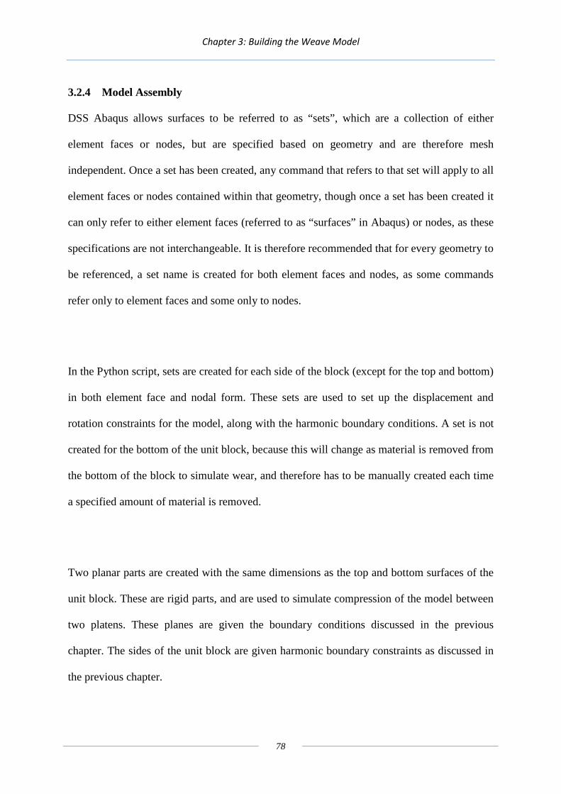
Chapter 3: Building the Weave Model
78
3.2.4 Model Assembly
DSS Abaqus allows surfaces to be referred to as “sets”, which are a collection of either
element faces or nodes, but are specified based on geometry and are therefore mesh
independent. Once a set has been created, any command that refers to that set will apply to all
element faces or nodes contained within that geometry, though once a set has been created it
can only refer to either element faces (referred to as “surfaces” in Abaqus) or nodes, as these
specifications are not interchangeable. It is therefore recommended that for every geometry to
be referenced, a set name is created for both element faces and nodes, as some commands
refer only to element faces and some only to nodes.
In the Python script, sets are created for each side of the block (except for the top and bottom)
in both element face and nodal form. These sets are used to set up the displacement and
rotation constraints for the model, along with the harmonic boundary conditions. A set is not
created for the bottom of the unit block, because this will change as material is removed from
the bottom of the block to simulate wear, and therefore has to be manually created each time
a specified amount of material is removed.
Two planar parts are created with the same dimensions as the top and bottom surfaces of the
unit block. These are rigid parts, and are used to simulate compression of the model between
two platens. These planes are given the boundary conditions discussed in the previous
chapter. The sides of the unit block are given harmonic boundary constraints as discussed in
the previous chapter.

Chapter 3: Building the Weave Model
79
Contact regions and the mesh must now be defined. Contact is not defined using the script as
this has to be redefined every time material is removed from the unit block to simulate wear,
and Abaqus CAE includes very simple commands for finding contact pairs based on
geometry which are sufficient for this model. The model also has to be re-meshed for
different levels of wear, and this is left for the user to perform. The mesh pattern at the
bottom contact surface must have a regular structure for use in the friction model, discussed
in the next chapter. This structure is shown in Figure 3.7. Each thread section is split in two
in the y-direction, as is every resin spacing section. Each warp thread is split in two in the x-
direction, and each weft thread section split into four in the y-direction.
Figure 3.7 Bottom side of unit cell with mesh pattern shown

Chapter 3: Building the Weave Model
80
3.3 Post-Python Tasks
As mentioned earlier, some tasks need to be performed manually after the Python script has
been used to prepare the model for analysis. Firstly, material must be removed from the
bottom of the unit cell if an amount of wear is to be simulated. This is done by creating a
block with the same dimensions as the bottom surface of the unit cell, and with a height equal
to the wear depth simulated. By placing this across the bottom of the unit cell, as shown in
Figure 3.8, and subtracting its geometry from the overall geometry, the size of the unit cell is
reduced. The bottom platen must then be relocated to the new position of the bottom surface,
and the set for the bottom of the unit cell must be manually re-defined.
The mesh pattern must also be manually specified. This is done by placing nodes on the
border of the unit cell, and allowing DSS Abaqus to build the mesh. Figure 3.9 shows the
placement of nodes to create the mesh shown in Figure 3.7.
Figure 3.8 Node placement on bottom surface of unit cell to specify mesh layout, node locations in pink

Chapter 3: Building the Weave Model
81
Finally, the analysis input file must be generated, then modified. DSS Abaqus allows most
output types to be selected from the GUI, however the friction model requires the x-axis and
z-axis coordinates of all nodes on the contact surface, along with the contact pressures at
these points to be available as output information. The following lines must therefore be
manually inserted at the end of the Abaqus analysis input text file, so that this information is
outputted as part of the analysis.
*CONTACT PRINT, NSET=Bottom-side, FREQ=1 CPRESS *NODE PRINT, NSET=Bottom-side, FREQ=1 COOR1, COOR3,

Chapter 3: Building the Weave Model
82
3.4 Results
When a constant pressure is applied across the top rigid plane in the model, contact pressures
are generated on the bottom surface of the model. The pressure at any point is dependent on
both the stiffness of the material in contact, and the material directly above the material in
contact. Figure 3.9 shows the contact pressure contour at three different levels of wear,
alongside a side view of the unit cell with the resin hidden showing the material removed
from the bottom. The contact pressures are normalised with respect to the maximum contact
pressure and are therefore independent of the force applied. High pressure regions are
encountered where there is a high proportion of stiff reinforcement either in the contact or
just away from the area in contact, with low pressure areas where there is a high proportion of
soft PTFE either in or just away from the contact. Areas with a high proportion of resin in the
contact tend to a normalised pressure of approximately 0.3. The long areas of low pressure in
the y-direction seen when there is no wear correspond to the soft PTFE warp threads,
however once a wear depth of 2∆ is achieved these strands have all been worn away and the
surface threads are now predominantly oriented in the x-direction.
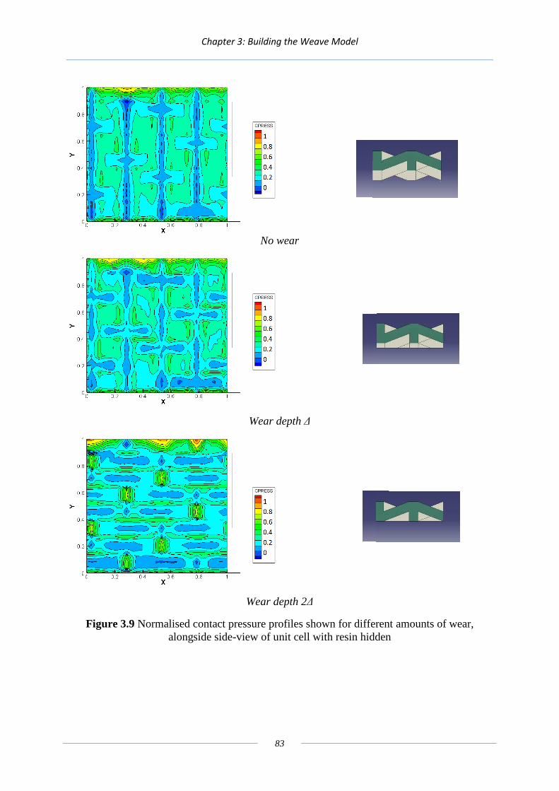
Chapter 3: Building the Weave Model
83
No wear
Wear depth ∆
Wear depth 2∆
Figure 3.9 Normalised contact pressure profiles shown for different amounts of wear, alongside side-view of unit cell with resin hidden

Chapter 3: Building the Weave Model
84
3.5 Technicalities of Python Script
3.5.1 Selecting Points
Selecting a section by coordinates is not an immediately obvious challenge. The most reliable
way of doing so involves calculating the coordinates of the centre of the section and using
this in a command to be applied to that section. Finding these coordinates however requires
additional calculation, and therefore increases the complexity of the script. An alternative
means of selecting a section is, if the coordinates of a point at the intersection between two
sections are known, to use the coordinates of the point at the intersection plus a small
increment to choose one of the sections. Figure 3.10 shows a datum point in red surrounded
by four surfaces. If the coordinates of the point in red are (0, 0), to select the top right section
(dark blue) would require reference to a point (0 + s, 0 + s), and to select the bottom right
section (light yellow) the coordinates would be (0 + s, 0 − s), where s is much smaller than
the dimensions of any section.
Figure 3.10 Datum point (red) surrounded by 4 surfaces (dark blue, light blue, yellow, light yellow)

Chapter 3: Building the Weave Model
85
3.5.2 Mesh resolution
The time necessary to perform a finite element analysis of a model is dependent on the
number of elements in the model, which for a given geometry depend upon the fineness of
the mesh. In this model, a compromise had to be found between a mesh which was
sufficiently fine as to produce a useful contact pressure contour, but with a realistic
computation time.
For a single variable, such as maximum displacement, a graph can be made of displacement
versus mesh resolution, and therefore a mesh which is sufficiently fine that the results are
independent of the mesh resolution can be found, and a finer mesh will not lead to a more
accurate result. In the case of a contour however, increasing the resolution of the mesh will
always increase the resolution of the contour on some scale, and as such the concept of a
mesh-independent result is less applicable to contours.
Figure 3.11 shows the contact pressure contour on the bottom surface of the unit block
without any material removed at three different mesh densities denoted as low, medium and
high density. By moving from a low-density to medium-density mesh it can be seen that more
detailed information is gained on the location of contact pressure peaks and valleys. In the
case of the high-density mesh information is not gained on the location of these peaks and
valleys, it is the definition of the boundaries between these areas that is increased. The low
mesh density allows the model to be analysed in less than ten minutes on the computer used
for these simulations, and the medium mesh density allows the model to be analysed in one

Chapter 3: Building the Weave Model
86
hour. The high mesh density model can take over four hours to analyse, and the trade-off
between increased resolution and increased processing time was not seen to be favourable.
The medium-density mesh was therefore adopted for generation of contact pressure contours
used in the friction model. Computation times are obviously dependent on hardware
specifications and additionally, since the development of this model, there have been
considerable improvements in the analysis speed of DSS Abaqus. As such, there is the
potential for future models to be meshed at much finer resolutions without necessarily
increasing the analysis time unduly.
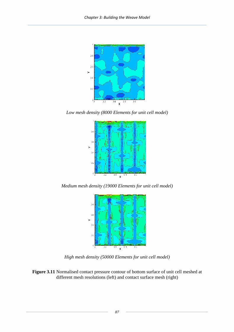
Chapter 3: Building the Weave Model
87
Low mesh density (8000 Elements for unit cell model)
Medium mesh density (19000 Elements for unit cell model)
High mesh density (50000 Elements for unit cell model)
Figure 3.11 Normalised contact pressure contour of bottom surface of unit cell meshed at different mesh resolutions (left) and contact surface mesh (right)

Chapter 3: Building the Weave Model
88
3.5.3 Omission of Reinforcement Layer
The test liner also has a further reinforcement backing layer. This has not been considered in
the analysis presented. In order to show that omission of the reinforcement layer in the finite
element model did not have any significant impact on results, a model was created which
included this layer, with all the same boundary conditions as the previously described model
of the test fabric alone. The thickness of this layer in the finished liner was obtained from
tomography. Figure 3.12 shows the finite element model assembly, with the test fabric in red
and the reinforcement layer in green.
Figure 3.12 Finite element model of test fabric and reinforcement layer, with the test fabric in red and the reinforcement layer in green
The reinforcement liner stiffness was given two values representing the lowest and highest
possible values. Three cases were compared; the test liner alone (case 0), the test liner with a
low stiffness reinforcement layer (case 1), and the test liner with a high stiffness
reinforcement layer (case 2)

Chapter 3: Building the Weave Model
89
To assess the effect of the inclusion of the reinforcement layer, the contact pressure contours
for the three cases were compared. Figures 3.13 and 3.14 show the results of these
simulations. In the case of these figures the differences in the results are extremely minor,
and can only be revealed either by very close inspection of the contact pressure contours or
examination of the raw data. For the higher wear depth presented in Figure 3.14, the
differences are more apparent, but in all cases there is less than a 10% variation in the contact
pressure values.
The inclusion of the reinforcement layer in the model increases the processing time of one
analysis by between 4× and 10×, as the interface between the reinforcement layer and the test
fabric considerably increases the complexity of the calculation. When the Case 1 and 2
contact pressure contours were used in the friction model, the difference in the overall
coefficient of friction obtained was less than 5%, meaning that omission of the reinforcement
layer was a reasonable assumption, given the consequent improvement in processing speed.

Chapter 3: Building the Weave Model
90
Figure 3.13 Comparison of contact pressure contours at zero wear for Case 0 (top), Case 1 (middle) and Case 2 (bottom)

Chapter 3: Building the Weave Model
91
Figure 3.14 Comparison of contact pressure contours at a high wear depth for Case 0 (top), Case 1 (middle) and Case 2 (bottom)

Chapter 3: Building the Weave Model
92

Chapter 4: Friction Model
93
4. Friction Model
4.1 Concept Overview
The central concept investigated using the friction model is that the overall coefficient of
friction of the composite liner is dependent upon the coefficients of friction of the different
materials in contact. It is further hypothesised that this overall coefficient of friction is
dependent upon the proportions of each material at the contact interface, and also upon the
way in which the contact pressure is distributed.
The model uses the previously discussed Finite Element (FE) analysis to obtain stiffness
information at varying wear states, which is then used to predict an overall friction coefficient
at defined states of wear.
The research is concerned with the test bearing liner, but the wear simulation model is
designed so that its application to liners with different combinations of materials is
straightforward. This will enable it to be used as a tool in material development – to minimise
both the time and resources necessary to develop future alternative bearing liner materials.
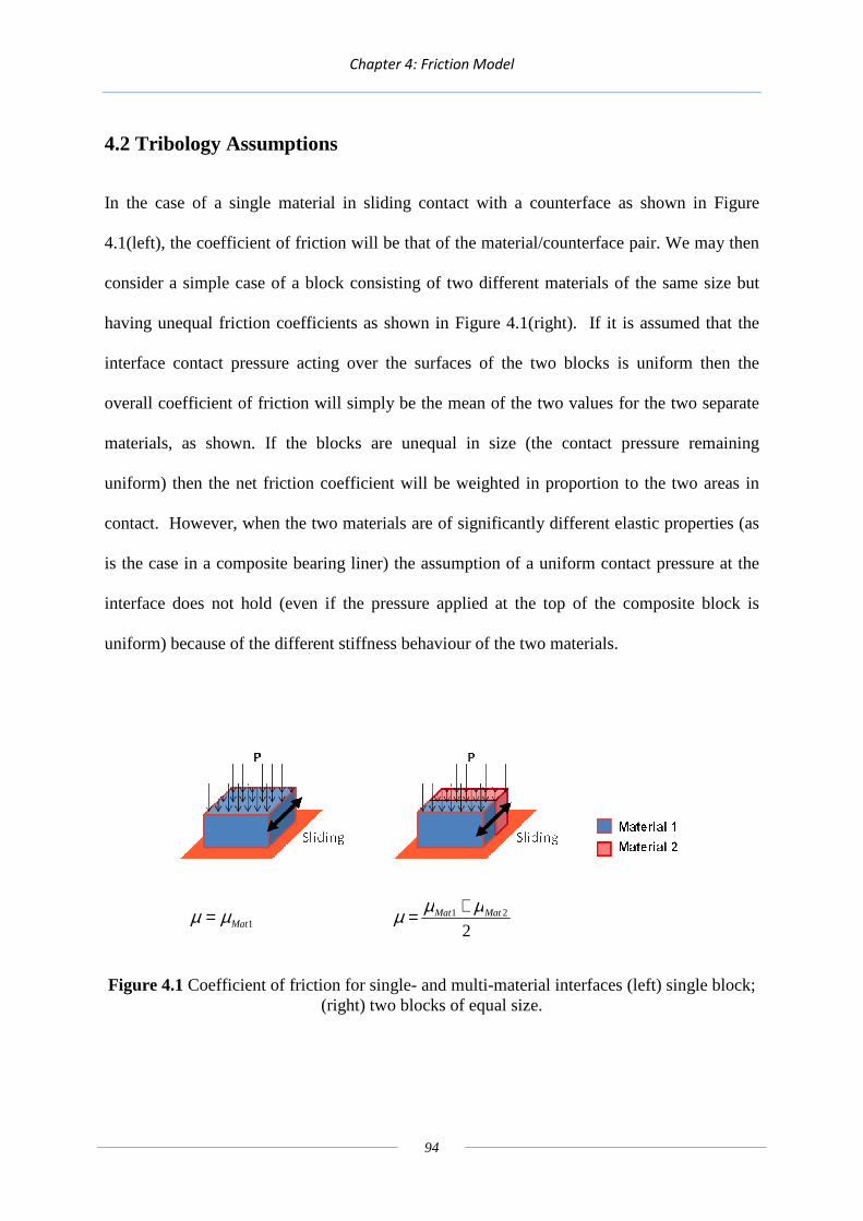
Chapter 4: Friction Model
94
4.2 Tribology Assumptions
In the case of a single material in sliding contact with a counterface as shown in Figure
4.1(left), the coefficient of friction will be that of the material/counterface pair. We may then
consider a simple case of a block consisting of two different materials of the same size but
having unequal friction coefficients as shown in Figure 4.1(right). If it is assumed that the
interface contact pressure acting over the surfaces of the two blocks is uniform then the
overall coefficient of friction will simply be the mean of the two values for the two separate
materials, as shown. If the blocks are unequal in size (the contact pressure remaining
uniform) then the net friction coefficient will be weighted in proportion to the two areas in
contact. However, when the two materials are of significantly different elastic properties (as
is the case in a composite bearing liner) the assumption of a uniform contact pressure at the
interface does not hold (even if the pressure applied at the top of the composite block is
uniform) because of the different stiffness behaviour of the two materials.
1Matµµ = 2
21 MatMat µµµ +=
Figure 4.1 Coefficient of friction for single- and multi-material interfaces (left) single block; (right) two blocks of equal size.

Chapter 4: Friction Model
95
Assuming that in the simple case of the 50/50 area split, one half is subjected to a very high
contact pressure, and the other half is subjected to little or no contact pressure, then the
overall coefficient of friction will tend towards that of the material with the highest contact
pressure. Figure 4.2, for example, shows a two-material block in sliding, with different
pressures applied to each section. Assuming that these pressures are transmitted directly to
the contact, and they are not re-distributed at the interface between the two materials, then the
net coefficient of friction will be given by Equation 4.1
Figure 4.2 A two-material block with different contact pressures on the two materials.
2211
222111~
pApA
pApAW
F friction
++== µµµ (4.1)
In the case of an n-material contact (such as the composite liner which consists of three
distinct materials) we make the fundamental assumption that the overall friction coefficient is
based on the area in contact of each material, and the contact pressures of those areas as

Chapter 4: Friction Model
96
follows:
nn
nnn
pApApA
pApApA
++++==
...
...
2211
222111~ µµµµ (4.2)
Finally, we must take account of the fact that in the composite liner considered the contact
pressure between each individual constituent material and the counterface will, in general,
vary from point to point (as revealed by the FE model) according to the geometry of the
textile weave and the proportions of different materials in the composite.
4.3 Principles
The simulation of friction and wear at the liner/counterface is based on the FE model. Values
are assumed for the elastic properties of the constituent materials together with their friction
coefficients when in contact with the steel interface. An overall coefficient of friction is
calculated for the liner/counterface pair at a range of wear depths, weighted according to the
proportions of each material in contact and contact pressures of the regions in contact as
outlined above.
The contact force at each node of the friction model is calculated by multiplying the contact
pressure at the node by its associated area. The frictional force at each node is then given by
the product of the force at that node and its associated coefficient of friction. The sum of
these frictional forces, divided by the area in contact, gives the effective coefficient of friction
for the contact interface, , shown in Equation 4.3

Chapter 4: Friction Model
97
nodenodecontactnode
nodenodenodecontact
FF
areapF
µ×=
×=
,
,
∑∑=
node
node
areaF~
µ (4.3)
It is important at this point to distinguish between two concepts – FE nodes and friction
model nodes. FE analysis makes use of elements, which in the case of the model developed
are either six-node or eight-node wedge and brick elements, respectively, with faces made up
of three or four nodes, as illustrated in Figure 4.3.
Figure 4.3 Node distribution on Wedge (left) and Brick (right) elements
Friction model nodes represent an area, specifically a rectangular contact face comprising of
a single material. Friction model nodes exist at the centre of the contact face of each FE
element, and have both an associated area and a contact pressure, as illustrated in Figure 4.4.
In an FE model, pressures (p) are applied at nodes, and friction coefficients (µ) are associated
with element faces. In the friction model, friction coefficients are applied over an area, and

Chapter 4: Friction Model
98
have an associated average pressure across the element area, p .
Figure 4.4 FE (left) and friction model (right) meshes of a given area
4.4 Abaqus Output Files
DSS Abaqus by default delivers results in a database file (.odb) which can be used to
visualise results through the Abaqus results visualisation module. Data can also be requested
for certain results in a tabular format, and this is done by adding this request to the Abaqus
processer input file. To request the data for a specific area, in this case the contact area, the
area of interest is manually selected in the user interface and given a name, so that it can then
be called in the input file.
The data required in this case are the coordinates of each FE node in contact, and the contact
pressure associated with each node. Forces are calculated in the FE model at nodes,
irrespective of whether a node-based or element-based contact formulation is used, and
contact pressures are obtained by dividing the force at the node by its associated area to
determine the nodal pressure. These data are then manually manipulated into a structure
FE Node
FE Element
Friction model Node
Friction model Node
(Associated Area)

Chapter 4: Friction Model
99
ready for use in the friction model, stored as a .csv file. Data are referred to by point number.
The point number is a method of referring to nodes without including the coordinates of the
point. Figure 4.5 shows an example of this numbering scheme. In this example the bottom
right node would have the coordinates (0.25, 0.05) and the point number (3,1).
Figure 4.5 Friction model mesh with dimensions (left) and node numbering scheme (right)
These files all have the same structure – the first three lines define the wear depth step and
the number of points in the x and y directions. The “wear step” is the notation used to define
an amount of wear, and is described in the next section. Each subsequent row is then made up
of five data items – the point number in x and then y, the x then y coordinate, and finally the
contact pressure at that node (in pascals). The final line is always five 0’s, to inform the
friction model code that it is the end of the file. Table 4.1 shows an illustration of this format,
along with an actual example in Table 4.2.
3
2
1
1 2 3
0.3
0.2
0.1
0 0.1 0.2 0.3

Chapter 4: Friction Model
100
Table 4.1 Layout of .csv file containing contact pressure data
Layer no.
No. Points
(x)
No. Points
(y)
Point no. (x) Point no. (y) X coordinate Y coordinate Contact Pressure
Point no. (x) Point no. (y) X coordinate Y coordinate Contact Pressure
Point no. (x) Point no. (y) X coordinate Y coordinate Contact Pressure
Point no. (x) Point no. (y) X coordinate Y coordinate Contact Pressure
… … … … …
… … … … …
0 0 0 0 0

Chapter 4: Friction Model
101
Table 4.2 Example of .csv file containing contact pressure data
2
25
33
1 33 0.3846 -1.17 0.2612
2 33 0.4346 -1.17 0.4569
3 33 0.4846 -1.17 1.48
4 33 0.5558 -1.17 1.732
… … … … …
… … … … …
0 0 0 0 0
The layer number in Table 4.1 is not read by the friction model code, and is there to allow
the user to see which wear depth a .csv file corresponds to without knowing its file name. The
number of points in the x and y dimensions are used to specify the size of the array that the
contact pressures will be read into. Currently the arrays are the same size for each wear step,
however this feature gives the potential for different mesh sizes to be used at different wear
steps.

Chapter 4: Friction Model
102
As seen above, the first three lines of each file contain data both for the user’s information
and to define the size of the arrays needed. These data are only read into the friction model
for the first wear step (all wear steps have identical meshes in the contact region); for all
other input files this code indicates to the friction model where to begin loading contact
pressure values into the .csv file.
4.5 Wear Steps
The friction model calculates overall friction coefficients corresponding to discrete amounts
of wear of the liner material, split into a series of wear “steps” ∆, where 8 ∆ is the maximum
wear depth considered for normal use. The reasons for choosing these particular wear
amounts are to maintain the same mesh pattern at the contact interface while removing
discrete amounts of material from the model.
The numerical procedure for simulation of wear effectively removes layer after layer from
the original surface of the composite liner thereby revealing different strata of the textile
weave. As each “wear step” progresses through the weave it therefore exposes surfaces with
different mixtures of the three components (reinforcement, PTFE, resin). This affects not
only the area-fraction occupied by each component, but also the way in which pressure is
distributed on the surface due to changes in the local stiffness behaviour of the liner when
loaded in the FE model.

Chapter 4: Friction Model
103
The wear simulation process, involving reductions in the volume of the model clearly has
implications for the FE element structure. If we consider a section of one of the PTFE yarns
in the warp/weft direction, for example, due to the pattern of the cell division it is possible to
remove discrete amounts of material while maintaining the mesh pattern. Figure 4.6 shows a
section of a weft thread with example mesh patterns at three different levels of wear. It can be
seen that in all cases there are four element faces on the bottom edge of the unit cell.
Figure 4.6 Single weft thread (top) with mesh pattern of the highlighted section shown at 3 different levels of material removal (bottom)
The figure shows that by using cuboid and wedge shaped elements, the same number of
elements in contact can be maintained despite the changed geometry. In the above example
the mesh is too coarse and would lead to mesh-dependent results, however these areas can be
broken down into smaller meshes to obtain a mesh-independent result while maintaining the
same number of elements in contact, as illustrated in Figure 4.7

Chapter 4: Friction Model
104
Figure 4.7 Actual mesh of section seen in Figure 4.6
4.6 Model Structure
The friction model utilises the contact pressure data generated by the FE model, along with
definitions of the materials in contact, and calculates an overall friction coefficient for the
material at different levels of wear based on the proportions of each material in contact and
the contact pressure variation. The model comprises of six parts, which are discussed in detail
in the following sections of the chapter. Figure 4.8 shows a flowchart which illustrates the
sequence in which these parts are handled..

Chapter 4: Friction Model
105
Figure 4.8 Friction model flowchart
4.6.1 Model Setup
This section sets up the variables used in the friction model, be they integers, real (decimal),
numbers or arrays, etc.
The friction model code begins by naming the executable file that will be created. It then
defines all variables used, be they numbers or arrays. For example, “sxl” and “syl” are the
dimensions of the friction model node arrays in x and y, and are defined as integers, as these
will later be read in from the Abaqus output files.

Chapter 4: Friction Model
106
The friction model defines one- and two-dimensional arrays, their size not being set at this
stage, as this is dependent on the data read in from the Abaqus output files. The one
dimensional arrays (sx, sy, sxa, sya) are used to calculate the size of the associated area for
each friction model node. The remaining arrays are used to define different information for
each wear step, with n denoting the integer value of the wear depth:
• Area of each friction model node (“area”)
• Young’s modulus at each friction model node (“youngs”)
• Contact pressure at each FE node (“cpressn”)
• Contact pressure at each friction model node (“cpresseln”)
• Friction coefficient at each friction model node (“coefn”)
• Force due to contact pressure at each friction model node (“forceeln”)
• Force due to friction at each friction model node (“fricforcen”)
• Force due to friction at each friction model node, assuming a non-varying contact
pressure distribution (“testfricmatn”)
4.6.2 Load External Inputs
The contact pressure distribution generated by the FE analysis must be prepared to be read in
from .csv files. These data must first be extracted from the FE results and processed into a
format appropriate to the friction model, as described in a previous section.
The blank, undimensioned arrays are then given their dimensions, in terms of the data read in
from the beginning of the Abaqus output files, in terms of “sxl” and “syl”. These are the

Chapter 4: Friction Model
107
number of nodes in the x- and y-directions, and therefore “sxl-1” and “syl-1” are the number
of friction model nodes in the x- and y-directions.
The data from the Abaqus output files are now read into the model. The contact pressures are
read into a contact pressure array for the current wear step, and, in the case of the first wear
step, the x- and y-coordinates of each FE node are also read, though this is necessary for
subsequent steps.
4.6.3 Format Data
By reading in the coordinates of all FE nodes, the size of the rectangle associated with the
friction model nodes can be calculated by finding the difference between the x- and y-
coordinate of each FE node and its neighbour. This is performed once for all wear steps, due
to their identical mesh patterns. Once the two arrays of x and y vertex lengths have been
calculated, they are multiplied together to give an array of the areas associated with each
friction model node. These values depend on the resolution of the coordinates tabulated by
the FE model, but the difference between the sum of all friction model node areas and the
actual total contact area is always less than 0.12%, therefore this is not seen as a source of
significant error.
As discussed earlier, in this model there will always be one more node in any axis direction in
the FE model than there will be in the friction model. Thus the size of any array of FE nodes

Chapter 4: Friction Model
108
has to be reduced by 1 in all dimensions to match it to the size of a friction model node array.
The matrix reduction is performed by taking an average of the four FE nodes which surround
the friction model node. This process reduces the resolution of the data, however a check is
included to compare the total contact pressure before and after the downsizing process, and in
all wear steps the difference between the total contact pressure before and after was less than
1%.
4.6.4 Define Materials
An array is also created for each individual wear step of the same dimensions, but containing
the coefficient of friction for each friction model node based on the material in contact at that
node. As no suitable method of transferring this information between the FE model and the
friction model code was identified, this array was built manually. The Abaqus graphical
interface is used to view materials definitions at elements, and this is transferred to the
Friction model code by specifying the material at each friction model node in the array.
4.6.5 Calculate Friction Coefficients
Once all the necessary arrays have been generated and filled, they are multiplied together as
according to Equation 4.3.
∑∑=
node
node
areaF~
µ (4.3)

Chapter 4: Friction Model
109
Two other “check” values are also calculated – the total tangential force at each wear step,
and an average area-weighted coefficient of friction for the material based on the areas in
contact and their coefficients of friction, but not the contact pressures, as seen in Equation
4.4.
∑= nodeFTotalForce
∑∑ ×=
node
nodenode
areaarea
Avg)(µµ (4.4)
A deviation in the total force would indicate that either not all contact pressures have been
read in correctly in that step, or there is a problem in the array reduction between FE contact
pressures and friction model contact pressures. The average coefficient of friction acts as a
benchmark for the overall coefficient of friction, and significant deviation between these
values could indicate a miscalculation within the friction model code and can be used to
prompt a checking investigation.
The values for the coefficient of friction for each wear step, with and without inclusion of the
contact pressure weighting, are then displayed to the user. These will vary based on the
coefficients of friction specified for each material in the contact, so careful consideration of
the values used is necessary

Chapter 4: Friction Model
110
4.7 Results
In order to produce a friction coefficient for a given wear step, coefficients of friction must be
defined for the three materials in contact. As the future application of the model was seen as
being for analysis of pre-prototype liner materials, deriving these values from bespoke tests
was not seen as appropriate. Instead values were taken from a commonly available source for
the stiffness and coefficients of friction of these three materials. Table 4.3 shows the values
assumed for the friction coefficient of each material.
Table 4.3 Friction coefficients of materials used in friction model (Engineering Toolbox, 2013)
Friction Coefficient
PTFE 0.04
Reinf. 0.2
Resin 0.6

Chapter 4: Friction Model
111
Figure 4.9 shows the variation in friction coefficient versus wear depth generated by the
friction model. There is an almost constant coefficient of friction of 0.18 until a wear depth of
4∆, at which stage the coefficient of friction increases significantly. This increase in the
coefficient of friction is attributed to the increase in the proportion of reinforcement in the
contact region. Figure 4.10 shows the variation in the proportion of each material in contact.
It can be seen that after a wear depth of 8∆, the proportion of reinforcement in the contact
region increases sharply.
Figure 4.9 Variation of friction coefficient with depth of wear predicted by the friction model

Chapter 4: Friction Model
112
Figure 4.10 Proportions of materials in contact at varying wear depths predicted by the friction model
The sensitivity of the results to the assumed coefficients of friction for each material was also
assessed by simulating each material successively with a friction coefficient of 1.0 and the
other two materials with coefficients of zero. Figure 4.11 shows the results of this analysis,
and demonstrates that the model is most highly sensitive to the coefficient of friction applied
to the resin, except in the case of a wear depth of 8∆ when it is most sensitive to the
coefficient of friction of the reinforcement.

Chapter 4: Friction Model
113
Figure 4.11 Results of sensitivity analysis of friction model
Figure 4.12 shows a comparison between the results obtained from the friction model with
and without taking account of the contact pressure variation across the interface. The values
without the contact pressure variation are easier to generate, as they only require knowledge
of the proportions of materials in the contact area at different wear depths.

Chapter 4: Friction Model
114
Figure 4.12 Results of friction model with and without contact pressure bias
4.8 Limitations
The friction model was originally meant to use contact pressure data from the FEA model at
element integration points (in this case the centre of the element), as this would match the
number of points with the size of the friction model mesh. A difficulty was found, however,
in obtaining the dimensions of the elements when the data were requested in this manner,
which meant the area of each element could not be used in the friction model. As a result the
information about contact pressures is read in at nodes, and the averaging process discussed
earlier is used to obtain the effective pressure acting on each element.
The friction model was originally intended to be highly flexible with regard to the number of

Chapter 4: Friction Model
115
wear steps used and mesh density of the FE/friction model models at each of these steps. The
final code is built on this principle, However, no reliable method for obtaining data about the
material assignment at the Abaqus elements in contact could be found which was available in
a useful format. The array defining the coefficient of friction of each friction model node
(based on the material it is associated with) is a key part of the model, and due to this
limitation it has to be created manually. This means that each extra wear step has to have this
array manually defined, and it also has to be redefined following any changes in mesh density
for existing wear steps.

Chapter 4: Friction Model
116

Chapter 6: Wear Model
159
6. Wear Model
6.1 Theory
The wear taking place in composite spherical plain bearings is in general a much simpler
process than the complex wear mechanisms found in lubricated rolling-element bearings. In
principle, the area of the bearing liner subjected to both load and sliding will wear away,
gradually increasing the conformity of the liner and the inner ball, thus distributing the load
over a wider contact patch. Figure 6.1 shows the constituent parts of a spherical plain bearing,
with the non-conformity between the inner ball and the outer ring exaggerated for clarity. The
three components considered are the inner ball, which will fit onto the reciprocating part of
the application via a shaft, the outer race, which will fit into a housing in the non-moving part
of the application, and a composite self-lubricating liner which resides between the two. This
is a typical arrangement, and other configurations where both the inner ball and the outer ring
are in motion can be reduced to this case by simply considering the relative motion of the
components. The bearing is subjected to a load, and the inner ring reciprocates with an
oscillation measured in degrees about the centre of the inner ball, and with a frequency in Hz.
Rotation about the axis normal to the axis of load application and the axis of reciprocation is
also possible. This is referred to as misalignment, and is a result of misalignment between
components in the overall assembly.

Chapter 6: Wear Model
160
Figure 6.1 Schematic arrangement of spherical plain bearing with exaggerated non-conformity between inner ball (grey) and outer ring (dark blue), also showing the composite
liner (light blue) and the load and reciprocation that the bearing is subjected to
The lifespan of a bearing is measured by the number of operating cycles under load until the
bearing is no longer suitable for the application. In the case of rolling element bearings, the
end of a bearing’s life is usually characterised by catastrophic failure, resulting in
significantly increased friction and often a structural failure of the overall bearing. In most
applications of spherical plain self-lubricating bearings, the bearing becomes unsuitable once
the clearance or “backlash” has reached a pre-determined limit. Backlash in this example is
the maximum radial internal clearance, defined as “The total free play between the ball and
the outer ring when measured in the radial direction, i.e., normal to the centreline of the
bearing bore.” (SAE, 2007)
A means of modelling the progression of backlash over the life of the bearing is sought both
Reciprocation
Misalignment

Chapter 6: Wear Model
161
for estimating the lifespan of a bearing in a given application, and predicting the effect of
changes in bearing geometry or operating conditions. In practice is is found that the majority
of wear takes place on the liner due to loss of material. Some wear is seen on the inner ball,
but this is invariably much less than that which takes place on the liner, and usually amounts
to a marginal change in surface roughness rather than a change in form. The inner ball and
outer race are manufactured from steel and these components are an order of magnitude
stiffer than the liner material in practice. In formulating a simple wear model therefore, the
liner may be treated as the deformable, wearable component sandwiched between rigid, non-
wearing parts.
In the wear model considered here, contact between the liner and inner ball is calculated
based on the liner’s elastic stiffness. Elastic deformation of the loaded liner is assumed to
behave according to a simple bedspring model (Johnson 1987) as illustrated in Figure 6.2.
The figure shows “springs” (initially all of the same length in this case) supporting the load
applied between a rigid curved body and a rigid flat. The springs are deflected to conform to
the shape of the rigid body, so that for a given translation of the rigid body, there will be a
variation in the deflection of the springs.

Chapter 6: Wear Model
162
Figure 6.2 2D bedspring model of a rigid circular object (blue) under load supported by a flat body represented by a series of springs, with the variation in deflection of the springs visible
In general all springs in a bedspring model have an associated length and stiffness, which
means that a given strain of a spring (L
L∆=ε ) will give a stress due to contact, herein
referred to as a contact pressure (L
LEcontact
∆=σ ). This contact pressure will be dependent on
the length (L) and stiffness (E) of the spring considered. By considering the equations for
stiffness and strain, εσ=E and
L
L∆=ε ,
L
LEcontact
∆=σ (6.1)
The product of the contact pressure of a spring and its associated area (A) gives the load
carried by that spring. For a flat bedspring model, the sum of the load carried by all springs
gives the total load carried.
∑∆=
allspringstotal L
LEAW (6.2)
The area and length of a spring is dependent on the geometry of the model, and its stiffness is
Load

Chapter 6: Wear Model
163
dependent on the properties of the material to be simulated. This means that if the deflection
of all springs in a model is known, the load applied to the rigid part in the model can be
calculated.
In order to create a model of a spherical bearing, a method of calculating the displacement of
the ball into the liner is necessary, which gives the variation in displacement of the liner
across the contact region. To calculate the displacement of the inner ball into the liner, the
concept of eccentricity was used as in journal bearing theory. In a journal bearing the
lubricant is oil; in a composite bearing the lubricant is solid, but the geometry of the space
between the rigid parts is the same.
Figure 6.3 shows a journal bearing, with the journal (grey) surrounded by a lubricant, with
the clearance between the journal and the bearing exaggerated. The clearance of the journal
bearing, c, is the difference between the radius of the bearing (Rb) and the radius of the
journal (Rj). The eccentricity of the journal, e, is the distance between the centre of the
journal (Oj) and the centre of the bearing (Ob). The gap between the journal and the bearing,
h(θ), varies dependent on its radial position, θ, which is the angle measured from the centre
of the journal. The minimum gap (hmin) and maximum gap (hmax) are found along the axis of
load application in the case where there is no reciprocation. The axis of translation is the
radial direction at the point where the gap is hmin, i.e. θ = 0. In the composite bearing
application this is also the direction of load application, as shown in Figure 6.3. (In a journal
bearing the axis joining the maximum/minimum clearances does not in general align with the
load axis due to the nature of the hydrodynamic lubrication mechanism which is governed by

Chapter 6: Wear Model
164
the Reynolds equation).
Figure 6.3 Diagram of journal bearing with lubricant, showing key components and dimensions
The eccentricity ratio, ε, is the eccentricity of the journal (e) divided by the radial clearance of
the bearing (c). The eccentricity of the bearing is typically a few orders of magnitude smaller
than the radius of the journal, so, as in hydrodynamic journal bearing theory, the gap between
the journal and the bearing at any angular position may be closely approximated by
)cos1()( θεθ += ch (6.3)
h(θ)
hmin
θ=0
θ
W
hmax
e
Oj
Ob
Lubricant
θ=π
Journal
Bearing

Chapter 6: Wear Model
165
6.2 Spherical Plain Bearing Liner Contact Model
6.2.1 Relationship between Contact Load and Eccentricity
This model is first applied to the case of a two-dimensional journal bearing with a self-
lubricating liner. In this case the gap, h(θ), is the distance between the journal and the outer
race at a given radial position. For a very small load, just enough to give contact, the distance
hmin would be the thickness of the liner, t. If a significant load is applied, W, this will cause
the liner to deflect in the contact region, and the minimum gap will be less than the thickness
of the liner. The deflection of points with gaps less than the thickness of the liner can be used
in Equation 6.1, along with the calculation of liner deflection at a point, )(θhtl −=∆ , to give
L
htEcontact
))(()(
θθσ −= (6.4)
By dividing the area in contact into a series of points or nodes, with the deflection known at
each of these points, a contact pressure contour can then be calculated.
For a flat bedspring model, the total load is found from the sum of all contact pressures
multiplied by the associated area covered by each spring. In the journal bearing case,
however, the spring axes are not parallel, therefore the load carried by each spring has to be
resolved into the direction of the axis of load application. Figure 6.4 shows a spring with a
gap of h(θ), highlighted in red, which is inclined at angle θ from the axis of load application.
If dA is the liner area corresponding to the spring, the amount of load carried along the axis of
load application, will be

Chapter 6: Wear Model
166
L
dAhtEW
))((cos
θθθ−= for h(θ) < t
0=θW for h(θ) ≥ t (6.5)
The total load carried by the liner will be, for all points with h(θ) less than the thickness of
the liner,
∑∑−−
−==π
π
π
πθ
θθL
dAhtEWWtotal
))((cos (6.6)
Equation 6.6 can be extended to the spherical case provided that θ is then treated as the solid
angle between the radial direction corresponding to area dA and the load direction.
Figure 6.4 Diagram of journal bearing adapted for self-lubricating liner, with a spring highlighted in red, and its associated radial position (θ) and gap (h(θ)) shown
h(θ)
hmin
θ=0
θ
W
hmax
e
Oj
Ob
Liner
θ=π
Journal
Outer Race

Chapter 6: Wear Model
167
6.2.2 Liner Contact Model Discretisation and Solution Method
By finding a solution to Equation 6.6 in three dimensions, we can calculate the load applied
to the inner ball for a given eccentricity ratio. The solution is simplified by defining some of
the variables according to the bearing quantities. The stiffness, E, is the stiffness of the liner,
and is based on either empirical evidence or data from a finite element analysis of the
material. The length of the springs, L, is the thickness of the liner, and the initial clearance, c,
is known from the geometry of the bearing specified. This leaves only the area associated
with the springs, A, the cosine of the solid angle between the spring and the load-line, cosθ,
and the eccentricity ratio, ε, to be found.
In order to solve the problem analytically, the liner is divided by a mesh – a series of points
(nodes) each with an associated area, material properties and representative geometry. In the
3D model, a mesh pattern is generated over the surface of the inner ball, and this mesh is then
projected onto the liner. As the clearance between the inner ball and outer race is very small
compared to the radius of the bearing, this is seen as an acceptable simplification. The mesh
contains a series of nodes at which h(θ) can be calculated. Nodes are defined by coordinates
in (z, α). The z-coordinate is the axial distance measured from the inner ring mid-plane, and
the α-coordinate is the rotation about the ring axis as defined in Figure 6.5. The z-coordinate
is the distance from the centreline (z = 0) to the point of intrest, and is positive to the left of
the centreline, and negative to the right. The α-coordinate is the angle measured from the line
of load application (α = 0) and is negative in the clockwise direction, and positive in the anti-
clockwise direction.

Chapter 6: Wear Model
168
Figure 6.5 Front- (left) and side-profile (right) of inner ring of spherical plain bearing, showing coordinate system and example point (AST Bearings, 2013)
The domain of z is –zmax< z < zmax, and the domain of α is –π < α < π. The mesh of nodes
divides the spherical surface of the inner ring in equal increments of z and α and this is
referred to as a regular mesh spacing, although the distance between mesh points and the
spherical surface is not uniform. In the z-dimension, the mesh is split into a series of nodes
with a spacing of ∆z in the z-direction. This quantity is calculated in the following manner,
z=0 α=0
zmax
+z
α
Front Side

Chapter 6: Wear Model
169
where nz is the number of divisions in the z dimension.
zn
zz max2
=∆ (6.7)
Nodes are required on the centreline, z = 0, so it is therefore necessary that nz is an odd
number. This is illustrated in Figure 6.6.
Figure 6.6 Front-profile of inner ring of spherical plain bearing, showing z-dimension mesh when nz=5, with nodes lying along dashed lines
In the α-dimension, a similar equation is used, with ∆α being the spacing between points in
radians, and nα the number of divisions in the α dimension. For a constant load direction
relative to a fixed outer race, contact can only occur on one half of the liner, irrespective of
movement of the inner ball, and for this case the domain of α was adjusted to –½π < α < ½π,
to significantly reduce the number of calculations. To allow the future potential for
dz dz ∆z ∆z ½∆z ½∆z ∆z ∆z
z = 0

Chapter 6: Wear Model
170
introduction of a moving load line however, αmax is left as an adjustable parameter.
α
παn
2=∆ (6.8)
Nodes are required on the centreline, α = 0, and do not extend to the far edge of the inner
ring. It is therefore also necessary that nα is an odd number. This mesh is illustrated in Figure
6.7.
Figure 6.7 Side-profile of inner ring of spherical plain bearing, showing α-dimensional mesh when nα=5, with nodes lying along dashed lines
Figure 6.8 shows the two meshes combined, with an example point highlighted in red and its
associated area highlighted in blue. The area associated with a node is half the distance to its
neighbouring nodes on all sides in both the z-axis direction and α-axis direction. In the case
of a flat plane with x- and y-axes, the area would be
A=(½dx+½dx) × ( ½dy+½dy)=dx dy (6.9)
α=0
∆α α=½π α=-½π
½∆α ½∆α
∆α ∆α ∆α

Chapter 6: Wear Model
171
This model is however spherical, and this spherical geometry must be taken into account
when determining the area associated with a node.
Figure 6.8 Node (red) with associated area highlighted (blue)
Due to the equal spacing of the mesh, each point will have the same associated area. The
sphere is divided into spherical segments in the z-dimension, which have a surface area of
2πRh, where R is the radius of the sphere and h is the height of the segment. This is illustrated
in Figure 6.9. In this model, the height of the segment is dz, and the radius of the sphere is the
radius of the outer race, Rout, minus the thickness of the liner, t. The area associated with a
node is therefore (Stojek & Osteryoung, 1989)
ztRA out ∆−∆= )(α (6.10)

Chapter 6: Wear Model
172
Figure 6.9 Key dimensions of spherical segment (Stojek & Osteryoung, 1989)
To derive a formula for calculating cosθ for all points, we consider two points on the surface
of the inner ball – P0, the point through which the load acts, and P, a general point of interest
– and the origin at the centre of the sphere, O. P0 has the coordinates (z0,α0) and P has the
coordinates (z,α). This is illustrated in Figure 6.10
Figure 6.10 Front- and side-profile of an inner ball showing points P (red) and P0 (blue) along with the associated dimensions of P0
α =0
α
P0
P
c
c
rp
z = 0
z
O
P0
P
rp
c
c
z
y
x
y
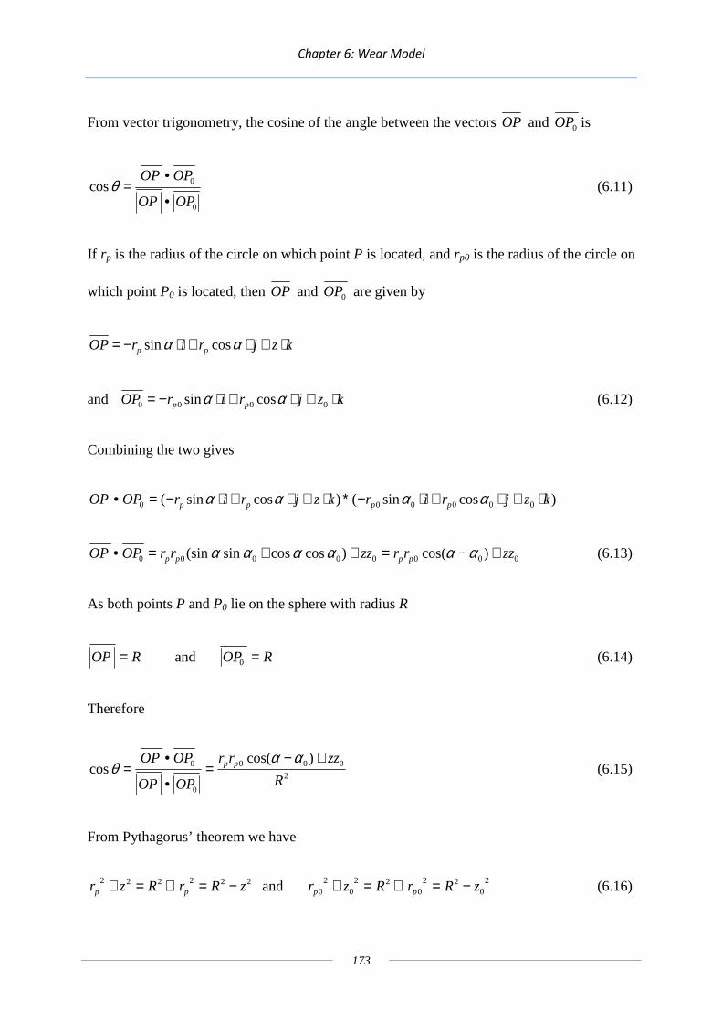
Chapter 6: Wear Model
173
From vector trigonometry, the cosine of the angle between the vectors OP and 0OP is
0
0cosOPOP
OPOP
•
•=θ (6.11)
If rp is the radius of the circle on which point P is located, and rp0 is the radius of the circle on
which point P0 is located, then OP and 0OP are given by
kzjrirOP pp ⋅+⋅+⋅−= αα cossin
and kzjrirOP pp ⋅+⋅+⋅−= 0000 cossin αα (6.12)
Combining the two gives
)cossin()cossin( 000000 kzjrirkzjrirOPOP pppp ⋅+⋅+⋅−∗⋅+⋅+⋅−=• αααα
00000000 )cos()coscossin(sin zzrrzzrrOPOP pppp +−=++=• αααααα (6.13)
As both points P and P0 lie on the sphere with radius R
ROP = and ROP =0 (6.14)
Therefore
2
000
0
0 )cos(cos
R
zzrr
OPOP
OPOP pp +−=
•
•=
ααθ (6.15)
From Pythagorus’ theorem we have
222222 zRrRzr pp −=∴=+ and 20
220
220
20 zRrRzr pp −=∴=+ (6.16)

Chapter 6: Wear Model
174
Therefore
2
002
0222
0
0)cos((
cosR
zzzRzR
OPOP
OPOP +−−•−=
•
•=
ααθ (6.17)
All necessary variables are now available to solve Equation 6.6, except for ε.
∑∑−−
−==π
π
π
πθ
θθL
dAhtEWWtotal
))((cos (6.6)
Equation 6.6 shows a direct relationship between Wtotal and ε . To find the eccentricity of the
inner ball for a given load ε is varied until the total load for all points is the same as the given
load, +/− an error percentage. This is carried out numerically by repeated division.
Two values for ε are initially created, εhigh and εlow, and are given the following initial values
c
tlow −= 1ε and 1=highε (6.18)
An ε value of 1 means that e/c is equal to 1, therefore the eccentricity is the same as the
clearance, meaning the inner ball has completely compressed the liner and has reached the
depth of the outer race at a point. εhigh is initially set to this value as, in this model, it is not
possible to have a higher eccentricity that the clearance of the bearing, as the outer race is
rigid and cannot deflect. For the case where the inner ball is just touching the liner (under
almost no load), the eccentricity of the inner ball is c−t, and as ε =e/c, this gives c
tlow −= 1ε .

Chapter 6: Wear Model
175
The total load is initially calculated at a value of ε exactly half way between εhigh and εlow. If
the load is found to be too high, εhigh is changed to the current ε value, and a new ε is found
between the new εhigh and εlow. If the load is too low, εlow is changed to the current ε value,
and a new ε is found between the new εhigh and εlow. This process is repeated until the ε value
gives the specified load, within a user-defined error margin.
6.2.3 Comparison of Liner Contact Model and equivalent Finite Element model
The simple bedspring model differs from a finite element model primarily due to the fact that
adjacent springs have no connection, unlike a finite element model where adjacent elements
are connected. This means that in a bedspring model only springs which are within the
contact area are deflected, whereas in a finite element model there is some deflection outside
of the contact area. For a given geometry and load the overall contact pressure contour was
compared between the bedspring model and a finite element model using DSS Abaqus
software. The model represents a steel spherical plain bearing having an inner ball radius of
20 mm and a steel outer race of radius 22 mm, with a 0.5 mm thick liner around the interior
of the outer race, with an assumed stiffness of 10 GPa. Figure 6.11 shows this geometry as
assumed in the finite element model. The finite element model is axi-symmetric and two-
dimensional, comprising of a rigid arc of 20 mm radius to represent the inner ball, and a 0.5
mm thick liner of outer radius 22 mm, with an encastre boundary condition along its outer
edge to represent the outer ring. The inner ball and outer ring are not represented as elastic
parts as their stiffness is an order of magnitude (>20×) larger than that of the liner. Both
models had a mesh applied such that there were at least 100 nodes in the contact region.

Chapter 6: Wear Model
176
Figure 6.11 Finite element model of journal bearing with self-lubricating liner
Figure 6.12 shows the results obtained from the the bedspring-based model and the finite
element model. The key differences are:
• The bedspring model contact pressures are distributed over a slightly smaller area.
This is to be expected as a limitation of the bedspring model is that it does not allow
for deflection (and therefore stress) outside of the contact region, whereas finite
element analysis does account for this effect. The difference in the contact dimension
is minor (<2%) and is therefore not seen to be significant.
• The bedspring model exhibits a higher contact pressure in the centre of the contact,
with a slightly lower contact pressure at the outer edge of the contact. This is due to
the difference in deflected shape between the liner in the liner contact model and

Chapter 6: Wear Model
177
finite element model, as shown in Figure 6.13.
The differences between the two models were small, and the bedspring model was seen to be
an acceptable approximation of the contact behaviour in the spherical plain bearing.
Figure 6.12 Comparison of results of finite element (FE) model with bedspring model for the assumed journal bearing geometry. The distance from centre is a radial distance, not a vector
distance in the x-axis/z-axis direction.
Note: The overall load integrated across the contact region appears to be higher for the bedspring model than the finite element model, however as this is a circular contact the load
should be integrated acrossπr2, which gives the two loads as equal to within 1%.

Chapter 6: Wear Model
178
Figure 6.13 Comparison of exaggerated deflected shape of liner between bedspring model (left) and finite element model (right)
6.3 Adding Wear to the Liner Contact Model
6.3.1 Overview
In Chapter 4 the effects of wear of the composite liner on contact pressure and net friction
were modelled by prescribing the wear process as one in which uniform layers of the surface
are removed to reveal different strata of the textile/resin mixture. The aim of the work
described in the following sections was to predict the instantaneous rate of wear of the liner
based upon an empirical wear model which assumes basic wear parameters for the individual
components of the composite. The wear model adopted is the simple Archard wear law as
follows
H
WLKQ = (6.20)
This equation gives Q, the total volume of wear debris (m3), dependent on W, the total normal
load, H, the hardness of the softer of the two contacting materials, K, a dimensionless
constant, and L, the sliding distance.
For an area of ∆A, the rate of change of liner thickness (dt/dζ, where t is liner thickness and ζ

Chapter 6: Wear Model
179
is time) will therefore be
AH
WuK
Adt
Q
d
dt
∆=
∆=
ζ (6.21)
Where u is the sliding speed (u=L/dζ) for area ∆A. W/∆A is the local pressure, p. From
equation 6.21 we then have
upH
KA
d
dt =∆ζ
(6.22)
Let ∆t be the depth of material removed per cycle. For a constant load, constant load direction
and a stationary outer ring we may write
∫=∆0
0
ζ
ζudH
Kpt (6.23)
Where ζ0 is the period of one cycle of oscillation. S, the sliding distance of the inner ball
relative to the liner position considered over one cycle of oscillation is
∫=0
0
ζ
ζudS (6.24)
Adding wear to the liner contact model involves varying the liner thickness at a given point to
simulate wear based on load and sliding distance, together with a modification of the pressure
distribution across the liner surface based on the change in thickness. Equation 6.25 shows
the contact pressure for a local liner thickness t. If we allow for changes in t, for a given

Chapter 6: Wear Model
180
displacement (h(θ)) contact pressure will increase as spring length decreases.
t
htEcontact
))(()(
θθσ −= (6.25)
By varying t in a controlled manner, and periodically recalculating the load distribution for
the modified spring lengths, it is possible to simulate wear in the bearing liner.
6.3.2 Sliding Distance
In order to determine the sliding distance of a point on the liner against the inner ring over a
cycle, we find the integral of the sliding speed (with respect to time) over the period of one
cycle. The sliding speed of the inner ring on the liner depends on the operating conditions, i.e.
the oscillation angle and frequency of oscillation in the reciprocation and misalignment
directions. In this model, only oscillation in the reciprocation direction is considered, as most
existing test data have been obtained using this motion.
The distance travelled by a point (u) moving around a circle or radius R byβ radians is
β⋅R (6.26)
Dependent on the position of a point which lies on a rotating sphere, the radius of the circle
on which it travels is equal to or less than the radius of the sphere, as highlighted in Figure
6.14. The radius of the circle, Rz, on which a point, P, lies in the z-axis direction is
determined by

Chapter 6: Wear Model
181
Rz2 + z2 = R2 therefore Rz
2 = R2 – z2 (6.27)
Where R is the radius of the inner ball, and z is the distance from the centreline of the point in
the z-axis, illustrated in Figure 6.14.
Figure 6.14 Front- and side-profile of an inner ball showing point P (red) and the radius of the circle on which it lies in the z-axis, Rz.
Oscillation in bearings is usually described as +/− Xo. This means that for a point lying
directly on the line of load, it will move Xo in one direction, then Xo back to its starting
position, then Xo in the opposite direction, then Xo to return to its starting position. This is the
movement undertaken in one cycle. For an oscillation angle +/− Xo, the total angular distance
travelled by the point will be 4 × Xo.
α=0
α
P
c
Rz
z=0
z
O
P
Rz
c
c c
z
y
x
y

Chapter 6: Wear Model
182
The total sliding distance over one cycle (S, in Equation 6.24) for a point with z-direction
dimension z, and oscillation of +/− Xo, on a sphere of radius R will therefore be
360
2422 π⋅⋅⋅−= oXzRS (6.28)
6.3.3 Wear Model Operation
Figure 6.15 shows how the wear of the bearing is determined computationally. The routine
runs in a closed loop, which continues to “wear” the liner until a pre-determined level of wear
has been reached.
Figure 6.15 Schematic of wear model routine
Deflection calculated for given load
and current geometry
Contact Pressure contour calculated
for current geometry
Sliding distance for cycle calculated
based on operation parameters
Material removed based on sliding
distance, contact pressure and local
stiffness
Worn geometry obtained
Process continues
until specified wear
depth achieved

Chapter 6: Wear Model
183
The Wear Model produces three key outputs: the wear profiles; contact pressure contours at
discrete intervals; and the progression of backlash through the bearing’s life. The “discrete
intervals” correspond to whole numbers of cycles which can be varied to increase or reduce
the number of data produced by the model.
The contact pressure profile is obtained for information only at this stage, but in future
applications of the model, where new materials may be under development, it may be helpful
as an indicator of pressure and temperature “hotspots”. The wear profile is output at discrete
numbers of cycles so that comparisons can be made to the wear profiles measured in actual
bearing tests.
6.4 Results and Comparison with Test Data
The results of the wear model may be compared with measured backlash values across the
life of a bearing. By using the same parameters as an actual bearing test for the motion, load
and geometry of a real bearing, results can be compared with bearing tests.
Bearing backlash values are usually monitored off-line during qualifying tests, i.e. a test has
to be stopped, and in some cases parts removed, in order to measure the backlash value. This
means that over the life of a bearing, there may only be one backlash value taken. A test rig
was used to monitor backlash values on-line whilst the test rig continued to operate. These
values do not compensate for the deformation of the liner due to load, as they are measured

Chapter 6: Wear Model
184
from the deflection of the inner ring. In these tests the bearings were run until the bearing
temperature reached a cut-off limit. It is not known at what locations these temperatures were
taken in the bearing. Both ambient and bearing temperatures were recorded over the course of
the tests, and three bearings were tested. Measured dynamic backlash values were obtained
periodically during the test and are presented in terms of the mean sliding distances at the
measurement intervals. The results of these tests are commercially confidential, consequently
some details of the test and wear model parameters are removed.
The wear model was given a set of conditions to closely match those of the bearings tested
physically. The bearing was assumed to be in perfect conformity with manufacturing
specifications – i.e. it met all tolerances. The simulation was allowed to run until the liner
was almost entirely worn (the maximum depth was 99% of its thickness), and the simulation
covered the range of wear allowed to take place in the actual tests. The stiffness was set to an
appropriate value, and the load matched to that of the physical tests, as were the frequency
and angle of oscillation in the radial direction. No oscillation in the misalignment direction
was included.
As no appropriate K value (the wear constant assumed in the Archard wear law) had yet been
found, this was set to 1×10⁻⁶, to ensure a high number of cycles to resolve the maximum wear
depth. The mesh density in the α and z directions was increased until increasing them further
showed no significant change in the results obtained. The load error margin (the difference
between the load calculated iteratively and the real load applied) was set at 0.01%.

Chapter 6: Wear Model
185
As the real bearing tests do not account for deflection of the liner, Figure 6.19 shows the
modelled deflection of the inner ring due to the combination of liner wear and liner
deflection. Wear depth is presented as a function of ∆, the “wear step” discussed in previous
chapters. As no appropriate K value was determined within the timeframe of the project, the
predicted deflection is shown plotted against sliding distance normalised with respect to total
sliding distance.
Figure 6.19 Inner ring deflection as a proportion of total sliding distance from the wear model
Figure 6.19 clearly shows the familiar two key features reported in both the literature and
observed in the real bearing tests discussed earlier. First, the “phase 2” linear wear rate
behaviour after 20% of its total sliding distance, and, second, the rapid increase in wear in

Chapter 6: Wear Model
186
“phase 1” before 20% of its total sliding distance. The simulation does not, however, exhibit
the “phase 3” wear out behaviour of a rapid increase in wear in the final 20% of the wear life.
Figure 6.20 shows the predictions of the wear model compared to the real bearing tests.
Figure 6.20 Real bearing test and wear model results showing inner ring deflection as a proportion of total sliding distance
Figure 6.20 shows that while the form of the results of the wear model is similar to the real
bearing tests in the first 80% of its total sliding distance (i.e. a slowing rate of increase of
wear with sliding distance), there is a difference in the magnitude of wear between the results
by a factor of about 2.5. This may be explained as follows. The wear model is allowed to

Chapter 6: Wear Model
187
wear to a much greater depth than is possible in real bearing tests, and the proportion of the
total sliding distance is a proportion of the sliding distance up to a wear of 30 ∆. From the
real bearing test data, Bearings 1 and 3 show that a wear depth of 5∆ is achieved at 60% of
the total sliding distance. All bearing test data and the wear model predictions were therefore
re-normalised, this time with sliding distance as a proportion of sliding distance to achieve 5∆
deflection, as shown in Figure 6.21.
Figure 6.21 Real bearing test and wear model results with inner ring deflection presented as a proportion of sliding distance to 5 ∆ inner ring deflection
The main difference between the wear model and real bearing test results are now seen to be
in the region of 70% to 100% final backlash. The real bearing tests show an increasing wear

Chapter 6: Wear Model
188
rate over this period which is not reflected in the wear model predictions. In real bearings,
this is believed to be the result of increased presence of reinforcement material in the contact
region, which increases the wear rate (as discussed in Chapter 1). The wear model however
does not have a variable wear rate, and the only attribute linked to the increase in
reinforcement material in the contact is the increase in localised stiffness.
The wear model exhibits the behaviour seen in the first two zones of the familiar three-zone
curve, discussed by King (1979) and others, which is encouraging. This correlation between
the wear model and the “knee” between zones one and two is of particular note as this feature
is commonly attributed to the development of a PTFE “transfer layer”, yet no information
regarding such effect is included in the model. While micrography of surfaces sliding with
PTFE do show the presence of such a transfer layer (Yang et al., 2009), some researchers
believe it to be developed extremely early in the wear process (Briscoe et al., 1988), long
before reaching ~20% of the total lifetime cycles. It is therefore hypothesised that this “knee”
is not the result of development of a PTFE transfer layer, but a geometrical effect of spherical
plain bearings. Initially there is very small load application region on the unworn bearing
liner, leading to high localised contact pressures and therefore wear rates. As the liner wears,
the load application region of the inner ball increases, reducing both localised contact
pressure and wear rate. The “wear out” transition between zones 2 and 3 on the real bearing
tests however could be a result of the failure of the transfer layer, leading to increased wear
rates. As the transfer layer (and its eventual failure) is not included in the wear model, this
could explain why the “wear out” feature is not seen in the wear model.

Chapter 7: Conclusions and Future Work
189
7. Conclusions and Future Work
7.1 Overview
The work described in this thesis was concerned with experimental measurement and
theoretical modelling of both friction and wear of a particular self-lubricating, composite
bearing liner material. A finite element-based friction model was developed which took
account of the detailed physical structure and elastic response of the PTFE/reinforcement
textile weave/resin filler composite liner loaded in contact with a steel counterface. The effect
of increasing wear on the contact and friction behaviour was modelled by progressively
removing layer after layer of the contacting face of the FE model to reveal different
proportions of the constituent materials of the composite in contact. In this way a net friction
versus wear depth graph was obtained. The friction coefficients of the individual components
of the composite assumed in the model were taken from both the literature and from values
actually measured in the test rig. The predicted net friction values using friction coefficients
from these two sources were then compared to the overall friction measured in a bespoke
friction and wear test rig. In general the predicted net friction values based on the individual
friction coefficients obtained from the literature were significantly higher than the
corresponding measured values. It was found that the calculation was particularly sensitive
to the friction coefficient of the resin filler, and closer agreement between predicted and
measured net friction was obtained assuming a (lower) friction coefficient actually measured
in the test rig using an isolated resin sample.

Chapter 7: Conclusions and Future Work
190
A numerical wear model for the composite liner was developed based on a simplified
“bedspring” formulation for the elastic behaviour of the liner in contact with the steel
counterface. The Archard wear law was adopted in an iterative scheme to predict the
progression of wear with sliding distance (under constant load), taking account of the
increased conformity and redistribution of contact pressure due to wear itself. The results
from the wear model were compared with the results of full-scale bearing tests carried out
earlier by SKF, and good agreement was obtained for the first 80% of the wear life of the
liner. The remaining sections of this chapter present a discussion of proposed future work on
the friction model, flat-on-flat coupon tests, and the bearing wear model, along with a
summary of the main conclusions of the thesis.
7.2 Aims and Objectives Met and Contributions
• A representative model of the liner material was created, which is both efficient and
useful.
• A friction model for the bearing liner was created. It was found that incorporating the
results of the finite element analysis did not increase the accuracy of the model, but
the model provides a useful prediction of the variation in coefficient of friction over
the operating life of the bearing liner provided appropriate coefficients of friction are
used for the constituent materials.
• Experimental data from the flat-on-flat wear testing rig was obtained, however due to
problems with the reliability of the rig, the data obtained were limited.

Chapter 7: Conclusions and Future Work
191
• A wear model was produced by adapting lubricated journal bearing theory, which
proved to be accurate for the first 80% of the wear life of a practical bearing liner.
• Results from the wear model show good agreement with the initial wear behaviour of
full-scale bearing tests without accounting for presence of PTFE. This suggests that
the formation of a PTFE transfer layer is not responsible for the transition between
initial and steady state wear behaviour as discussed in relevant literature, and that the
transition is in fact a geometric effect.
7.3 Future Work – Friction Model
The friction model showed encouraging results when appropriate coefficients of friction were
assumed for the constituent materials and when the reciprocating sliding distance amplitude
was greater than 25 mm. The model matches the steady-state (i.e. constant wear rate) period
of the trend of friction coefficient over the wear life of the bearing liner, and also the spike in
friction coefficient seen in some test results. It is notable that the method of predicting the
friction coefficient without the inclusion of the detailed elastic contact pressure distribution
provides good agreement with the experimental results, as this method is significantly
simpler to implement than that which calculates the pressure contours across the contact
surface. There was a lack of agreement in the results when the reciprocating sliding
amplitude is less than 25 mm. As discussed in Chapter 5, the particularly low coefficient of
friction seen with a sliding distance of 12.5 mm could be due to either the formation and
maintenance of a PTFE “transfer layer”, or possibly a thermal effect in the contact region.
Suggestions for the investigation of this effect are discussed in Section 7.3. To account for

Chapter 7: Conclusions and Future Work
192
the impact of these effects on the coefficient of friction, some form of sliding amplitude
based parameter should be included in the model. In the experimental testing it was also
noted that lower mean contact pressure resulted in a higher steady-state coefficient of friction,
therefore it may be necessary to include some degree of pressure-dependence in the values of
the individual friction coefficients of the constituent materials in future work.
The current model should be validated using other dry-sliding materials. This would require
further testing on the existing flat-on-flat coupon test rig. It would be desirable for this
material to either have the same structure as the current material, but with one material
changed (for example the resin), or for it to contain exactly the same materials, but in a
different weave structure, perhaps. This would help identify the variables which most affect
the model predictions and hence the real bearing behaviour.
Other factors which were not investigated experimentally in this project include the effect of
counterface surface roughness and humidity. These are factors which have been identified in
the literature review as having a significant effect on the coefficient of friction of liner
materials. These factors are both discussed further in Section 7.3, but including them in the
friction model would require further parameters to be considered.
The friction model should be developed to model friction in full-scale bearings over a range
of operating conditions. This would require development of a full FE model of the bearing
liner and the two spherical components in order to yield the extent of the zone of contact and

Chapter 7: Conclusions and Future Work
193
the detailed pressure distribution under load.
It was noted in Chapter 1 that “bearing torque” (or overall bearing friction) is generally
higher under “no-load” conditions, where a pre-load is introduced by manufacturing an
“overclosure” which ensures that new bearings have an initial contact pressure which is
relaxed as backlash develops due to wear. In this case inclusion of a contact pressure
dependency on the friction coefficient would allow comparison between loaded and un-
loaded bearing friction. If the concept of a critical sliding distance is also included, this
would allow identification of bearing geometries which may be inappropriate or inefficient in
a given application. For a given load and angle of oscillation, for example, reducing the
diameter of the bearing (subject to available load capacity, of course) also reduces the
circumferential sliding distance, therefore by reducing the diameter of the bearing, it is
possible in some applications that the coefficient of friction of the bearing will also be
reduced. The current friction model developed in this project is therefore a useful starting
point for the development of a more comprehensive model for industrial design purposes.
7.4 Future Work – Experimental Data
As discussed in Chapter 5, the number of data obtained from the flat-on-flat coupon test rig
within the timeframe of this project was limited. It is suggested that test regime D in
particular requires further investigation, as this showed a significantly reduced steady-state
coefficient of friction. Further investigation into the relationship between coefficient of
friction and pressure should also be carried out, as this relationship can be combined with

Chapter 7: Conclusions and Future Work
194
calculated contact pressure contours across the liner in real bearing geometries to give an
estimation of bearing friction under a range of loading conditions.
If, in the light of further testing, the results of test D1 are shown not to be anomalous, then
further tests using sliding distances between that of test C and test D should be carried out to
investigate the sliding-distance related transition between the two steady-state coefficients of
friction. It has been proposed that there may be a critical reciprocating sliding amplitude,
below which the friction coefficient attains a significantly reduced plateau value. An
alternative hypothesis is that below the critical sliding distance, the coefficient of friction is
lowered as sliding distance reduces further. This second hypothesis is thought to be less
likely, as the coefficient of friction of ~0.035 seen in test D1 is similar to that observed in
full-scale bearing tests (Henninger, 2011) and, importantly, in coupon fretting tests of the
material, which have very low sliding distances (Dayot, 2011). The proposed concept of a
critical sliding amplitude associated with a significantly reduced steady-state coefficient of
friction should also be investigated with regard to whether it is contact-pressure dependent or
not.
If a critical sliding distance exists, the next step is to investigate whether it is due to thermal
effects or the formation of a third body transfer layer. Options could include introducing a
heating element to the counterface artificially to generate a high temperature close to the
contact region. Of course the thermal/third body effects are not mutually exclusive – high
contact temperatures could aid the formation of the third body film, although in this case this
would still present the thermal effect as the governing variable, as a useful third body film

Chapter 7: Conclusions and Future Work
195
could not be formed without a sufficiently high temperature. Another method of evaluating
the two effects exclusively would be to run a test until the steady-state coefficient of friction
has been reached, then stop the test for a sufficient time to allow cooling back down to
ambient temperature, then start the test again. In this case it could be assumed that the third
body film had been formed, and was still present when the test was restarted. If the
coefficient of friction on restarting was found to be higher, that would suggest that the
temperature was not high enough to make the third body effective as a solid lubricant. If the
coefficient of friction was unchanged, it would imply that the formation of the third body film
was the governing factor in reducing the coefficient of friction.
As stated earlier, the impact of counterface roughness was not investigated with regard to
modification of the wear rate or steady-state coefficient of friction of the samples. It was
noted in Chapter 1 that some published work implies a critical roughness for minimum wear
rate, and that if the initial roughnesses is above or below this critical value, the roughness will
tend to this critical roughness over the course of the wear life of the material. This effect is
seen in Chapter 5, where three different counterface roughnesses were tested. Papers in the
literature suggest that this critical roughness is in the region of 0.05 µm Ra, whereas the
testing carried out in this project indicates a value of around 0.22 µm Ra. Ra is not however
an all-encompassing means of quantifying the functional significance of surface roughness
however, as it does not account for form or the presence (or otherwise) of isolated, high
asperity peaks, therefore detailed analysis of the surface using profilometry is needed to
understand the important surface parameters affecting performance.
Chapter 7: Conclusions and Future Work
196
Humidity was highlighted in Chapter 1 as a key factor in the friction of composite bearing
liners, however the test rig used in these experiments does not have the capacity to either
record or control the local humidity. As the tests in this project were carried out over the
course of three years, there will have been fluctuations in the local humidity, both daily and
seasonal. It is proposed that, in future work, a method of recording local humidity be included
on the test rig, as recording this fluctuation could, perhaps, be used to explain the spread of
results in the same test for both friction and wear performance.
7.5 Future Work – Wear Model
In order to make the wear model useful as a means of predicting the wear of a given bearing
geometry, an appropriate K value (dimensionless constant of wear) must be found. This value
should be obtained from experimental testing, and would hopefully be found to be uniform
across a wide range of bearing geometries. This would mean that the wear model in its
current form could be adopted as an aid for predicting wear of a given bearing geometry for
at least the first 80% of its wear life.
The model should be further developed in order to predict the trend of wear over the last 20%
of the bearing liner life. If the rapid increase in wear rate in this tertiary period is due to an
increase in the proportion of reinforcement in the contact region, a K value could be used
which varies dependent on the proportion of reinforcement calculated to be in the contact
region from models of the material. Inclusion of this feature is possible through use of the
tools already developed in this project.

Chapter 7: Conclusions and Future Work
197
In the current wear model, the stiffness of the liner is taken to be a fixed value. It should be
possible to modify the model so that the stiffness changes with wear. In the case of the test
liner, the softest materials are predominantly in the contact region of the unworn liner,
meaning the liner becomes stiffer as it is worn.
By knowing the load and wear depth of points across the spherical plain bearing contact
interface, it would be possible to make a prediction of the overall friction coefficient of the
bearing and show the progression of this friction coefficient over the bearing’s wear life. This
would require information on the load/friction coefficient behaviour for different wear
depths, which was not available given the time span of the project. Once this information is
available and has been validated, integrating this into the wear model would be a useful
additional feature.
A fully developed and experimentally verified bearing friction and wear model is an
ambitious objective. In the case of customer applications it could be used as an advanced
method of selecting the correct bearing geometry for the given application. As an aid in the
development of new materials, it could be applied as a preliminary screening method for
candidate materials, thus reducing the time spent in carrying out expensive testing.

Chapter 7: Conclusions and Future Work
198
7.6 Summary of Conclusions
• The friction and wear of self-lubricating bearing liners are affected by a range of
factors governed by both the operating and environmental conditions.
• Composite 3D textile weaves can be modelled in an efficient manner when reasonable
engineering approximations are made with regard to their structure.
• The friction model which has been developed is particularly sensitive to the
coefficient of friction used for the resin material and care must therefore be exercised
in determining this quantity.
• When an appropriate set of coefficients of friction are used for the constituent
materials in the friction model, a good approximation is made of the friction
behaviour over the bearing liner’s life when compared to experimental results from
coupon tests.
• Coupon tests of the coefficient of friction of the bearing liner suggest a dependence on
contact pressure and oscillatory sliding distance.
• When the liner is subjected to a uniform contact pressure, its wear rate is found to be
linear throughout its wear life.
• The wear model using the continuum mechanics approach gives a good
approximation of the wear behaviour of full-scale bearing tests over the first 80% of
their wear life and has potential for further development and improvement as a useful
design aid.

199
References
AST Bearings, 2013, “Steel-on-Bronze Series SPB” [online], [Accessed 12-01-2013], Available from: http://www.astbearings.com/steel-on-bronze-spb.html
Bell, A., 2009, “ARD511: Wear Hypothesis for SKF Airframe Self-lubricating bearing technology”, SKF Ltd.
Bell, A., 2012a, Private Communication.
Bell, A., 2012b, Private Communication.
Bell, A., 2013, Private Communication.
Bennett, A, 2008, “ARD498: Liner Compressive Stiffness Analysis”, SKF Ltd.
Bernard, P., 2011, “Discrete Modelling of Woven Structures”, SKF Ltd.
Bortoleto, E.M., Rovani, A.C., Seriacopi, V., Profito, F.J., Zachariadis, D.C., Machado, I.F., Sinatora, A., Souza, R.M., 2013, “Experimental and numerical analysis of dry contact in the pin on disc test”, Wear, v.301, pp. 19-26.
Bowman, D., Balch, J., Artaxo, P., 2009, “Fire in the Earth system”, Science. v. 324, pp. 481–4.
Bramham, R.W., King, R.B., Lancaster, J.K., 1980, “Fluid Contamination Effects on the Wear of PTFE-Containg Dry Bearings”, ASLE Prep 80LC6B3.

200
Briscoe, B.J., Evans, P.D., Lancaster, J.K., 1988, “The influence of debris inclusion on abrasive wear relationships of PTFE”, Wear, v. 124, pp. 177-194.
Brossard, I., 1997, “Technologie des Textiles” (in French), Dunod, Paris.
Callister, W.D., 2007, “Materials Science and Engineering – An Introduction” John Wiley & Sons.
Cao, L., Shen, X., Li, R., 2010, “Three-dimensional Thermal Analysis of Spherical Plain Bearings with Self-lubricating Fabric Liner”, Advanced Materials Research, v. 97, pp. 3366-3370.
Carnes, K., 2005, “The Ten Greatest Events in Tribology History”, STLE.
Cook, J.G., 1968, “Handbook of Textile Fibres 2 – Man-made fibres” Merrow Publishing, Watford.
Dayot, C., 2011, “Wear Scenario of a Bearing Liner”, SKF Ltd.
Department of Education and Science, 1966, “Lubrication (Tribology) Education and Research. A Report on the Present Position and Industries’ Needs”, HMSO, London.
Dowson, D., 1979, “History of Tribology”, Longman Ltd.
DSS Abaqus, 2012, “Analysis User’s Manual”.
Engineering Toolbox, 2013, “The Engineering Toolbox”, [online], [Accessed 12-01-2013], Available from: http:// http://www.engineeringtoolbox.com/

201
Eto, E., 2008, “Barnsdall Weaving Class” [online], [Accessed 12-01-2013], Available from: http://www.supercozy.com/blog/2008_08_01_supercozy_archive.html
Evans, D.C., 1978, “The friction and wear properties of PTFE composites at elevated temperatures”, RAE Tech. Report 77070, Royal Aircraft Establishment, Farnborough.
Evans, D.C., 1978, “Polymer-fluid interactions in relation to wear”, Proc. 3rd Leeds-Lon Symp. on Wear of Non-metallic Materials.
Fillot, N, Iordanoff, I, Berthier, Y, 2005, “Simulation of Wear through Mass Balance in a Dry Contact”, ASME Journal of Tribology, v. 127, pp. 230-237.
Floquet, A., Play, D., Godet, M., 1977, “Surface Temperatures in Distributed Contacts, Application to Bearing Design”, ASME Journal of Lubrication Technology, v. 99, pp. 277-283.
Floquet, A, Play, D, 1981, “Contact Temperature in Dry Bearings. Three Dimensional Theory and Verification”, ASME Journal of Lubrication Technology, v. 103, pp. 243-251.
Godet, M., Play, D., 1975, “Third-body formation and elimination on carbon-fibre/epoxy composite”, Space tribology proceedings of the first European Space Tribology, Fracasti, Italy, p.165-173.
Godet, M., Play, D., Berthe, D., 1980, “An attempt to provide a unified treatment of tribology through load carrying capacity, transport, and continuum mechanics”, Journal of Lubrication Technology, v. 102, pp. 153-164.
Holmberg, K., Matthews, A., Ronkaninen, H., 1997, “The Tribological Mechanisms of Coated Surfaces”, ASME Journal of Tribology, v.2, pp. 615-622.

202
Johnson, K.L., 1987, “Contact Mechanics”, Cambridge University Press.
Kennedy, F.E., Smidhammar, L., Play, D., 1975, “Wear of polyethylene in small-amplitude oscillatory motion”, Proc. 4th Eur. Trib. Congress, v. 2, pp. 1-9.
King, R. B., 1979, “Wear Properties of Dry Bearing Liners at Ambient and Elevated Temperatures”, Wear, v. 56, pp. 37-53.
Lancaster, J. K., 1972, “Lubrication of carbon fibre-reinforced polymers. Part 1 Water and aqueous solutions”, Wear, v. 2, pp. 315-333.
Lancaster, J. K., 1979, “Accelerated Wear Testing of PTFE Composite Bearing Materials”, Tribology International, v. 12, pp.65-75.
Lancaster J.K., 1981, “On the initial stages of wear of dry-bearing composites”, Ministry of Defence.
Lancaster, J.K., 1982, “Accelerated wear testing as an aid to failure diagnosis and materials selection”, Tribology International, v. 15, pp. 323-329.
Lancaster, J.K., Bramham, R. W., Play, D., Waghorne, R., 1982, “Effect of Amplitude of Oscillation on the Wear of Dry Bearings containing PTFE”, ASME Journal of Lubrication Technology, v. 104, pp. 559-568.
Li, J., Ran, Y., 2010 “Evaluation of the friction and wear properties of PTFE composites filled with glass and carbon fiber”, Materialwissenschaft und Werkstofftechnik, v. 41, pp. 115-118.

203
Li, K., Shen, X. J., Chen, Y., Li, R., 2008, “Numerical Analysis of Woven Fabric Composites Lubricated Spherical Plain Bearings”, Proc. 11th Intl Congress, Soc. For Experimental Mechanics Inc.
Liu, Z., Shen, X., 2010, “Study on the Elastic Properties of the Woven Fabric Liner of Spherical Plain Bearing with Self-lubricating”, Advanced Materials Research, v. 139, pp. 190-193.
Moreno, R., 2012, “What does shape function mean in finite element modelling?” [online], [Accessed 12-01-2013], Available from: http://stochasticandlagrangian.blogspot.co.uk/2011/07/what-does-shape-function-mean-in-finite.html
Moreton, R., 1983, “The wear behaviour of PTFE-based composite materials at different relative humidities”, RAE Technical Memo.
Morgan, J.E., Plumbridge, W.J., 1987, “The effect of humidity on dry bearing torque”, Wear, v. 119, pp. 215-223.
Parsons, E., Weerasooriya, T., Sarva, S., Socrate, S., 2010, “Impact of Woven Fabric: Experiments and Mesostructure-Based Continuum-Level Simulations”, Journal of Mechanics and Physics of Solids, v. 58, pp. 1995-2021.
Pihtili, H., Tosun, N., 2002, “Effect of load and speed on the wear behaviour of woven glass fabrics and aramid fibre-reinforced composites”, Wear, v. 252, pp. 979-984.
Pihtili, H., 2009, “An experimental investigation of wear of glass fibre-epoxy resin and glass fibre-polyester resin composite materials”, European Polymer Journal, v. 45, pp. 149-154
Play, D., Godet, M., 1977, “Self-Protection of High Wear Materials”, ASLE Transactions, v. 22, pp. 56-64.

204
Play, D., Pruvost, B., 1984, “Comparative dry Wear of PTFE Liner Bearing in Cylindrical and Spherical Geometry”, ASME Journal of Tribology, v. 106, pp. 185-193.
Play, D., 1985, “Mutual Overlap Coefficient and Wear debris motion in dry oscillating friction and wear tests”, ASLE Transactions, v. 28, pp. 527-535.
Puso, M., 2006, “A stabilized nodally integrated tetrahedral”, International Journal of Numerical Methods in Engineering, v. 67, pp. 841-867.
Python, 2013, “Python Programming Language – Official Website”, [online], [Accessed 12-01-2013], Available from: http://www.python.org/
Richard, D, Iordanoff, I, Berthier, Y, Renouf, M, Fillot, N, 2007, “Friction Coefficient as a Macroscopic View of Local Dissipation”, ASME Journal of Tribology, v. 129, pp. 829-835.
Richard, D, Iordanoff, I, Renouf, M, Berthier, Y, 2008, “Thermal Study of the Dry Sliding Contact with Third Body Presence”, ASME Journal of Tribology, v. 130, pp. 031404.1-031404.10.
Rossi, C., Russo, Fe., Russo, Fl., 2009, "Ancient Engineers' Inventions: Precursors of the Present”, Springer, pp. 171.
SAE, 1998, “AS81820 - Bearings, Plain, Self-Aligning, Self-Lubricating, Low Speed Oscillation”, SAE International.
SAE, 2007, ”Aerospace Recommended Practice”, SAE International.
Santner, E., Czichos, H., 1989, "Tribology of Polymers", Tribology International, v. 22, pp. 103-109.
205
Siede, G, 2012, “Research at ITA: Polymers”, [online], [Accessed 12-01-2013], Available from: http://www.ita.rwth-aachen.de/andere_sprachen/englisch/3-06-polymers.html
SKF Group, 2010, “SKF Spherical Plain Bearings and Rod Ends”.
Sliney, H. E., Williams F. J., 1982, “Performance of PTFE-Lined Composite Journal Bearings”, Ann. Meeting of the Am. Soc. of Lubrication Engr.,; 10-13 May 1982; Cincinnati, OH; United States.
Stojek, Z., Osteryoung, J., 1989, “Experimental Determination of the Coefficient in the Steady State Current Equation for Spherical Segment Microelectrodes”, Office of Naval Research.
Texgen, 2013, “Main Page”, [online], [Accessed 12-01-2013], Available from: http://texgen.sourceforge.net/index.php/Main_Page
U.S. Customs and Border Protection (U.S.C.P.B.), 2012, “What Every Member of the Trade Community Should Know About: The Classification of Ball Bearings, Roller Bearings and Parts Thereof”, Informed Compliance.
US Navy, 1998, “MIL-B-81820F - Bearings, Plain, Self-Aligning, Self-Lubricating, Low Speed Oscillation”.
US Navy, 2000, “MIL-B-81819B - Bearings, Plain, Self-Lubricating, Self-Aligning, High Speed Oscillation”.
Verma, A.P., Vishwanath, B., Kameswara Rao, C.V.S., 1996, “Effect of resin modification on friction and wear of phenolic composites”, Wear, v. 193, pp. 193-198.

206
Wagner, J., 2010, “New Formaldehyde Regulations Are Headed Your Way” [online], [Accessed 12-01-2013], Available from: http://www.propelmg.com/blog/2010/08/new-formaldehyde-regulations-are-headed-your-way/
Yang, Y., Ma, C., Huang, S., Jing, L., Pang, H., 2010, “Effects of Mechanical Properties of Kevlar/PTFE Fabric-Reinforced Self-lubricating Liners on Performance of Self-lubricating Spherical Plain Bearings”, Applied Mechanics and Materials, v. 29, pp. 197-202.
Yang, Y., Zu, D., Zhang, R., QI, X., 2009, “Effects of Friction Heat on the Tribological Properties of the Woven Self-lubricating Liner”, Chinese Journal of Mechanical Engineering, v. 22, pp. 918-927.