fringe tracking status - harvard university

IOTA-Ames Fringe Tracking Status Edward Wilson 21 February 2002 p 1/26

IOTA-Ames Fringe Tracking Status

Edward Wilson [email protected]

Intellization Smart Systems Research Lab, Information Sciences Division

NASA Ames Research Center

21 Feb 2002

Abstract This document summarizes the results of the integration effort from 2/11-15/02 at IOTA and overall progress to date. The fringe-tracking algorithm originally developed in 1998-1999 was improved and ported to ANSI C. With the assistance of Ettore Pedretti, it was integrated with the DAQ_Scheduler.cpp code written at IOTA, and successfully tracked fringes generated by a simulated light source. Weather prevented testing on the sky. The algorithm runs in 1.2 milliseconds per scan on the real-time PowerPC processor. With a slight reduction in accuracy and robustness, this time can be reduced to 0.17 ms per scan if needed. The C source code has been delivered to IOTA. This report discusses three major areas of development so far:

1. Identification of fringe packet center and integration at IOTA 2. Simulation of effect of atmospheric turbulence on optical path difference (initial attempts) 3. Prediction of fringe packet motion (using a linear model so far)

1. Identification of fringe packet center and integration at IOTA The fringe-tracking algorithm originally developed in 1998-1999 is described in the brief paper from ICO 18 [Wilson 1999], listed in Appendix B. It was developed and tested using about 4000 scans taken at IOTA in 1997, which are described in Appendix A. Using that algorithm, we are able to automatically identify fringe packet parameters to accuracy as good as can be determined by eye. That is, we can find fringe packet parameters (center, amplitude, spread of sinc function, frequency of fringes, and phase shift of fringes – or A, B, C, D, E in the model y = A sinc(B(x+C)) cos(D(x+E))) that appear to be the “best” match to the actual data. The first four steps (listed in the paper) find an initial estimate of the fringe packet center. This is what Sebastien Morel implemented at IOTA in 1999 (he converted the MATLAB code to C, then to Labview for implementation). Although the identification of fringe centers worked well, delays in the control loop caused the overall fringe-tracking system to fail. The remaining steps use an FFT and nonlinear gradient-based optimization of the fringe packet parameters. These steps take about 200% longer to compute, and produce only a small improvement in fringe-packet-center identification. For the 4000-scan 1997 data set, the maximum difference between initial and final estimates over all the data was 1.6 steps, standard deviation was 0.5 steps. The improvement in center-estimation (C) alone probably does not warrant implementing the full estimation (ABCDE), since the random motion of the fringe packet center is roughly 20 times larger than this improvement. Full estimation may be useful, however, for prediction of fringe packet motion – initial tests show that past and present values of fringe frequency, D, are useful for predicting future values of interferogram center, C. The remainder of Section 1 focuses only on this initial center identification, and does not discuss the full ABCDE identification.


1.1 Fringe tracking algorithm Since 1999, the initial center-identification algorithm has changed to the following, which appears to give excellent results (as the former one did) and is more physically based, so we expect it to be more robust for future data and algorithm changes:

1. A window (nominally of a length containing two fringe periods) is passed over the data, where a single-frequency discrete Fourier transform (DFT) is calculated to try to detect the expected fringe frequency (this frequency is adaptively updated – by changing the window size - after each scan).

2. The center of the interferogram is then found by:

a. Convolving a template (--- ++++++++ ---) with the DFT result from step 1 that is designed and sized to produce a high output when a peak is found. This is the same as the 1999 algorithm, but the width of the center part (+++) of the template was doubled.

b. The symmetry of the convolution result is calculated and used as another factor in finding

the center. The following 9 figures show an example of this algorithm’s application to a scan from data set 0 in the 1997 data set:

50 100 150 200 250

-0.3

-0.25

-0.2

-0.15

-0.1

-0.05

0

0.05

0.1

0.15

sample number []

no

rmal

ized

dat

a (A

-B)/

(A+B

) []

Raw scan data

raw scan dataidentified center

Figure 1

Figure 1 shows the raw data (combined using (A -B)/(A+B)), as well as the result of the center identification that came after all steps were completed.


110 115 120 125 130 135 140-0.4

-0.3

-0.2

-0.1

0

0.1

0.2

0.3

sample number []

no

rmal

ized

dat

a (A

-B)/

(A+B

) []

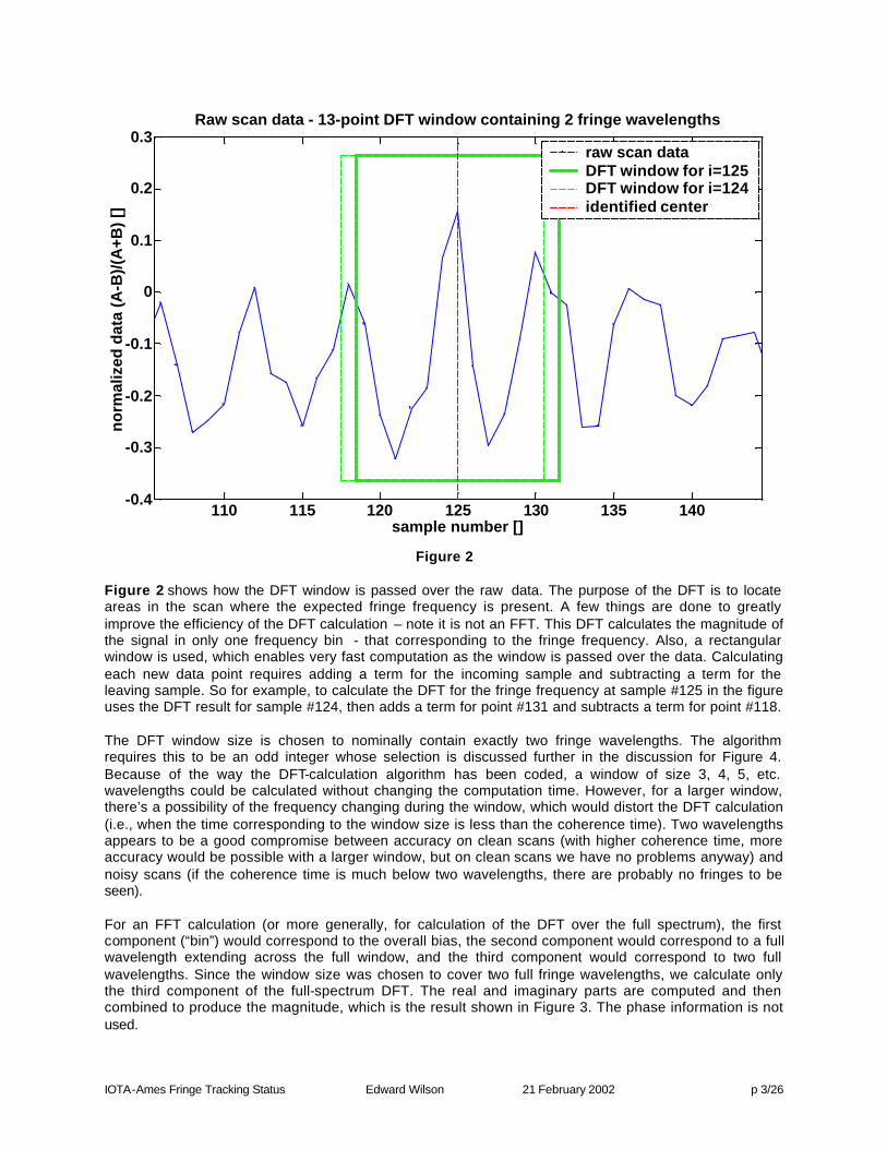
Raw scan data - 13-point DFT window containing 2 fringe wavelengths

raw scan dataDFT window for i=125DFT window for i=124identified center

Figure 2

Figure 2 shows how the DFT window is passed over the raw data. The purpose of the DFT is to locate areas in the scan where the expected fringe frequency is present. A few things are done to greatly improve the efficiency of the DFT calculation – note it is not an FFT. This DFT calculates the magnitude of the signal in only one frequency bin - that corresponding to the fringe frequency. Also, a rectangular window is used, which enables very fast computation as the window is passed over the data. Calculating each new data point requires adding a term for the incoming sample and subtracting a term for the leaving sample. So for example, to calculate the DFT for the fringe frequency at sample #125 in the figure uses the DFT result for sample #124, then adds a term for point #131 and subtracts a term for point #118. The DFT window size is chosen to nominally contain exactly two fringe wavelengths. The algorithm requires this to be an odd integer whose selection is discussed further in the discussion for Figure 4. Because of the way the DFT-calculation algorithm has been coded, a window of size 3, 4, 5, etc. wavelengths could be calculated without changing the computation time. However, for a larger window, there’s a possibility of the frequency changing during the window, which would distort the DFT calculation (i.e., when the time corresponding to the window size is less than the coherence time). Two wavelengths appears to be a good compromise between accuracy on clean scans (with higher coherence time, more accuracy would be possible with a larger window, but on clean scans we have no problems anyway) and noisy scans (if the coherence time is much below two wavelengths, there are probably no fringes to be seen). For an FFT calculation (or more generally, for calculation of the DFT over the full spectrum), the first component (“bin”) would correspond to the overall bias, the second component would correspond to a full wavelength extending across the full window, and the third component would correspond to two full wavelengths. Since the window size was chosen to cover two full fringe wavelengths, we calculate only the third component of the full-spectrum DFT. The real and imaginary parts are computed and then combined to produce the magnitude, which is the result shown in Figure 3. The phase information is not used.


0 50 100 150 200 2500

0.2

0.4

0.6

0.8

1

1.2

1.4

sample number []

DF

T m

agn

itu

de

[]Magnitude of 13-point DFT calculated at each point in the scan

DFT resultidentified center

Figure 3

Figure 3 shows the result of the DFT calculation. So, for example, the value at sample #125 (which happens to also be the identified center) was calculated using samples #119 through #131, and corresponds to a wavelength of 6 samples. Even though it is calculated very differently, this result is very similar to that resulting from the envelope-finding calculations described in the ICO 18 paper. As mentioned earlier, although the envelope-finding calculations provided excellent results, this DFT calculation is more physically based and is expected to provide better robustness for noisy signals that we have not been able to test on so far. Because the window size is 13, the first and last six points are set to zero since they are not calculated using a full window. The code was originally written to make these calculations, but it was found that when calculated using fewer points, these calculations could be noise-sensitive and throw off the rest of the algorithm. Figure 4 shows the result of the DFT calculation using three different window sizes. Since the fringe frequency is not known exactly, and may change, this algorithm adapts to use the best window size. For every scan, the DFT calculation runs three times: once for the window size used on the previous scan, once for 2 larger, and once for 2 smaller. The window size (n_dft, as shown in the plot legend, is the number of samples) corresponding to the highest DFT value (in this case, the highest DFT result occurs for n_dft = 13 at sample #127) is chosen and used for the remaining calculations for this scan and is carried through to the next scan as the middle window size. To prevent n_dft from increasing or decreasing too rapidly during periods of low signal-to-noise ratio, only one step up or down can be made per scan.


0 50 100 150 200 2500

0.2

0.4

0.6

0.8

1

1.2

1.4

sample number []

DF

T r

esu

lt fo

r w

ind

ow

siz

e =

no

min

al +

/- 2

Size of DFT window is checked on each scan

n_dft = 11n_dft = 13n_dft = 15

Figure 4

The DFT can be thought of as a sampled version (exists only at the bin frequencies) of the discrete- time Fourier transform (DTFT) of the continuous signal convolved with the DTFT of the window function (in the simplest case, as we have here, this is a uniform window of finite length). With an infinitely wide window, the DTFT of the window would be an impulse, so the convolution would not distort the DTFT of the signal. With a finite window, two effects occur:

1. Reduced resolution - unlike an impulse, the main lobe of the window function has some finite width. Convolving this with the signal DTFT may make it impossible to resolve between two frequency components.

2. Leakage - the component at one frequency leaks into that at another component due to the spectral smearing.

If the goal is to measure the DTFT of the signal, then ideally you'd like a window with a DTFT of a thin main lobe and small side lobes, but usually you trade off between the two. A rectangular window has a relatively narrow main lobe, while Hanning, etc. windows have a wider main lobe (worse), but have smaller side lobes (better). No matter the shape of the window, the main lobe gets narrower as the number of points in the DFT increases. For non-stationary signals as we have here, at some point you don't want to increase the window size because the frequency content is changing. In this case, the length and shape of the window are chosen so that the Fourier transform of the window is narrow in frequency compared with changes in the FT of the signal. [Oppenheim & Schafer] However, in this application, we are not so concerned with resolution or leakage since our target, the fringe frequency, is changing from scan to scan and within a scan. Reduced resolution actually helps insulate the result from these variations. As long as we adapt to these changes, the DFT result is useful for fringe tracking. This robustness to the exact frequency can been seen by the fact that the DFT results for the three different window sizes in Figure 4 are similar – any one of the could have been used for fringe tracking.


0 50 100 150 200 250-1

-0.8

-0.6

-0.4

-0.2

0

0.2

0.4

0.6

0.8

1

sample number []

No

rmal

ized

DF

T m

agn

itud

e []

Packet-finding template is convolved over DFT result, shown here at packet center

DFT resultTemplateidentified center

Figure 5

Figure 5 illustrates how a template is convolved with the DFT result. The template is very simple, composed of ones, zeros, and minus-ones, leading to very efficient computation. It is modeled after what the ideal DFT result should look like. The computation is efficient, since after the initial computation for the first sample, each additional sample calculation involves only 3 adds and 3 subtracts (no multiplies or divides) – corresponding to the six vertical edges on the template. The +1 region corresponds approximately to the width at half the maximum DFT result. The –1 regions on either side correspond to the locations where the sinc() function crosses zero. In a more ideal DFT result, the DFT result approaches zero at these locations. The overall width of this template is passed to the fringe tracking function as an input variable (nFringe), although performance appears to be very robust to this number. For example, a value of nFringe = 35 for the half-width (meaning the template spans 71 samples) was used to track simulated fringes at IOTA with the scan set to both 30 and 15 microns (the 15-micron scan had a fringe packet twice as wide as that of the 30-micron scan). Figure 6 shows the results of this template convolved with the DFT result. In the next step, shown in Figure 7, the symmetry of the DFT result is calculated at each sample. The idea is that in addition to having high frequency content at the fringe frequency, the fringe packet should be symmetric, so symmetry is measured. For perfect symmetry, at each sample, the nFringe samples to the left would have the exact same values as the (flipped) nFringe samples to the right. The sum of the devi ation from perfect symmetry is calculated at each sample. It was found that flat regions away from the fringe could score high on this symmetry measurement, so the value is normalized by dividing it by the sum of the values being tested (from i-nFringe to i+nFringe). Unlike the other steps in this algorithm, an efficient implementation has not been developed. For this reason, symmetry calculation alone takes about 66% of the total compute time. This is discussed further in Section 1.4.


0 50 100 150 200 250-5

0

5

10

15

20

25

30

35

sample number []

con

volv

ed D

FT

mag

nit

ud

e []

Result of convolution of Packet-finding template with DFT result

template convolution resultidentified center

Figure 6

0 50 100 150 200 2500

0.1

0.2

0.3

0.4

0.5

0.6

0.7

0.8

0.9

1

sample number []

sym

met

ry fa

cto

r []

Symmetry factor calculated on DFT result (lower = more symmetric)

symmetry factoridentified center

Figure 7


0 50 100 150 200 250-100

-50

0

50

100

150

200

250

300

350

400

sample number []

tem

pla

te r

esu

lt /

sym

met

ry r

esu

lt []

Template result / symmetry result - peak is used to determine packet center

template / symmetry resultidentified center

Figure 8

Figure 8 shows how the packet-finding template convolution result is combined with the symmetry factor result. The former is divided by the latter to produce the plot shown. The index corresponding to the maximum value of this result is used as the packet center estimate. These last two steps shown in Figures 7 and 8 have been found to improve center identification by a few samples in some cases, but are not strictly necessary. If compute time becomes an issue, they would be the first things to go.


0 50 100 150 200 2500

0.2

0.4

0.6

0.8

1

1.2

1.4

mean(DFT)=0.12319

mean(DFT)=0.79999

mean(DFT)=0.10948

DFT ratio = center / min(left,right)

= 0.79999 / min(0.12319,0.10948)

= 7.3073

sample number []

DF

T m

agn

itu

de

[]Calculation of confidence metric, dft_ratio = 7.3073


Figure 9

Once the fringe packet center has been identified, a decision must be made as to whether it is a valid identification and should be used to update the scan-center position. In cases where the fringe packet disappears momentarily, it is better to do nothing (keep scanning in the same location) than to chase the noise. This calculation is shown graphically in Figure 9. The concept is that the DFT calculation near the identified center should have a measurably higher value than the DFT calculation on the background noise. The mean of the DFT in windows spanning 20% of the scan width is calculated at the left edge, right edge, and at the identified center – as shown by the blue rectangles in the figure. The ratio of the mean DFT at the cent er to the smaller of the two edge measurements must be greater than a specified threshold. The reason to take both edges and then use the minimum is that this will give a valid background measurement even if the fringe falls at the edge of the scan. The associated windows and calculations are shown in Figure 9. Setting the threshold value will depend on the level of tracking accuracy desired, the relative scan width, and other factors. It is a balance between the cost of accepting a wrong estimate and ignoring a valid one – these costs vary depending on the application. A completely different but useful confidence measure, suggested by Ettore Pedretti, is to do the fringe tracking calculation for all three fringe packets (A-B, A-C, B-C). The level of consistency of the identified center for each fringe packet could be used as a confidence measure.


0 50 100 150 200 250-0.6

-0.5

-0.4

-0.3

-0.2

-0.1

0

0.1

0.2

sample number []

no

rmal

ized

dat

a (A

-B)/

(A+B

) []

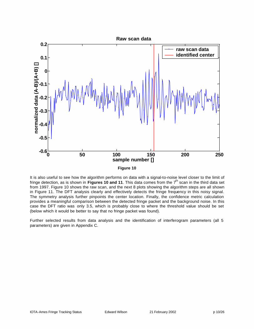
Raw scan data

raw scan dataidentified center

Figure 10

It is also useful to see how the algorithm performs on data with a signal-to-noise level closer to the limit of fringe detection, as is shown in Figures 10 and 11. This data comes from the 7th scan in the third data set from 1997. Figure 10 shows the raw scan, and the next 8 plots showing the algorithm steps are all shown in Figure 11. The DFT analysis clearly and effectively detects the fringe frequency in this noisy signal. The symmetry analysis further pinpoints the center location. Finally, the confidence metric calculation provides a meaningful comparison between the detected fringe packet and the background noise. In this case the DFT ratio was only 3.5, which is probably close to where the threshold value should be set (below which it would be better to say that no fringe packet was found). Further selected results from data analysis and the identification of interferogram parameters (all 5 parameters) are given in Appendix C.


0 50 100 150 200 2500

0.5

1

1.5

sample number []

DF

T r

esu

lt f

or

win

do

w s

ize

= n

om

inal

+/-

2

Size of DFT window is checked on each scan

n_dft = 11n_dft = 13n_dft = 15

140 145 150 155 160 165 170-1

-0.5

0

0.5

sample number []

norm

aliz

ed d

ata

(A-B

)/(A

+B)

[]Raw scan data - 11-point DFT window containing 2 fringe wavelengths

raw scan dataDFT window for i=155DFT window for i=154identified center

0 50 100 150 200 2500

0.5

1

1.5

sample number []

DFT

mag

nitu

de [

]

Magnitude of 11-point DFT calculated at each point in the scan


0 50 100 150 200 250-1

-0.5

0

0.5

1

sample number []

No

rmal

ized

DF

T m

agn

itu

de

[]

Packet-finding template is convolved over DFT result

DFT resultTemplateidentified center

0 50 100 150 200 2500

5

10

15

20

25

30

sample number []

conv

olve

d D

FT m

agni

tude

[]

Result of convolution of Packet-finding template with DFT result

template convolution resultidentified center

0 50 100 150 200 2500

0.2

0.4

0.6

0.8

1

sample number []

sym

met

ry fa

cto

r []

Symmetry factor calculated on DFT result (lower = more symmetric)

symmetry factoridentified center

0 50 100 150 200 2500

50

100

150

200

250

300

sample number []

tem

plat

e re

sult

/ sy

mm

etry

res

ult

[]

Template result / symmetry result - peak is used to determine packet center

template / symmetry resultidentified center

0 50 100 150 200 2500

0.5

1

1.5

mean(DFT)=0.1908

mean(DFT)=0.67718

mean(DFT)=0.20071

DFT ratio = center / min(left,right) = 0.67718 / min(0.1908,0.20071) = 3.5492

sample number []

DF

T m

agn

itu

de

[]

Calculation of confidence metric, dft_ratio = 3.5492


Figure 11


1.2 Implementation in C The algorithm was developed using MATLAB, which was also used to generate all the plots in this report. Since the tracker needs to run on a VxWorks processor (Motorola PowerPC 604 processor on a MVME-2431 card), after the initial prototyping in MATLAB, the algorithm was converted (manually) to C. As the algorithm evolved during this implementation process, the MATLAB and C versions were continually updated to maintain the same variable names, function names, and structure to the extent possible. The two versions produce results that are identical when compared to the limit of floating point precision (6 digits). A test function was developed in both C and MATLAB that generated an idealized scan for testing the algorithm. This arrangement proved useful in determining whether a problem was in the interface between the calling function (in DAQ_Scheduler.cpp), the implementation of the C-version of the function (ptracker_ed()), or the algorithm itself (in which case a problem would be detected when running in MATLAB). This development arrangement will enable off-line data analysis and facilitate further algorithm improvements. The C code is compiled using WindRiver Tornado, which uses the gcc compiler to create a .out file that is then loaded onto the VxWorks target at run-time. The scan control code, in DAQ_Scheduler.cpp includes a reference to the code as:

/**************************************************** * This is the packet tracker callable from DAQ_Scheduler.cpp * the returned value is 1 if a packet was found successfully, otherwise 0 * y_raw_double is a pointer to an array of doubles - the raw (normalized) data * nl and nh are the index limits of that array, e.g. 0 and 127 or 1 and 256, etc. * n_dft is a pointer to an integer containing the number of points used in the * DFT window. It must be an odd number, and should equal the number of * data points in two wavelengths of the fringe (13 is a good initial guess). * It is updated by the function, so it should be kept alive for use * on the next scan. * nFringe is a pointer to an integer containing the number of samples from the * center of an ideal fringe packet to where the sinc function crosses 0. * Recommended setting = 35. Capability to adaptively set this within * ptracker_ed() may be added, which is why it is a pointer. Alternatively, * analysis external to ptracker_ed() could be used. * threshold_ratio, a float, is the limit for comparing max(y_dft) (an internal variable) * with the dft readings away from the detected fringe packet. If this calculated * ratio > threshold_ratio, the returned value will be 1, indicating * that a packet was found. Recommended setting = 5.0 * centerPhase is a pointer to a float containing the phase angle of the identified * center of the fringe packet. -pi corresponds to the very first data point in * the scan, and +pi corresponds to the last one. ****************************************************/ extern "C" { int ptracker_ed(double *y_raw_double, unsigned long nl, unsigned long nh, int *n_dft, int *nFringe, float threshold_ratio, float *centerPhase); }

Tornado uses the g++ compiler to compile DAQ_Scheduler.cpp, and the “extern “C” {" in the declaration enables it to call the C function. Variables that may need to be changed, such as nFringe, n_dft, and threshold_ratio, are passed as inputs to this function so that there should not be a need to recompile the fringe-tracking code if these parameters must be updated for different observing conditions. These parameters can be set through the IDL interface, enabling them to be changed easily during a run. This fits nicely into a proposed implementation architecture in which this algorithm and Ettore Pedretti’s fringe-tracking algorithms can be tested against one another or used together. The second (or third) tracking algorithms can be encoded similarly to this one. Then the DAQ_Scheduler program can switch


between them on the fly, either using a command from the IDL-shared-memory interface for testing, or an internal logic calculation for determining which tracker should be used on a particular scan. 1.3 Testing After the algorithm was successfully updated and integrated during the week of February 11-16, 2002, it was tested on the IOTA system, tracking fringes generated by a light source. Tracking performance was very good, even with temporary loss of fringe data (for example, caused by banging the table) – in these cases, the system correctly decided that confidence was low and did not try to track until the fringe packet re-formed. Also, the system performed very well with the scan travel set at both 15 and 30 microns, and with no manual adjustment of parameters. The fringe packet appears twice as wide for the 15-micron scan, further indicating the robustness of the algorithm. Unfortunately, due to poor weather conditions, we were unable to test it on the sky. When initially implemented, some overshoot was noticed when the fringe tracking was active. This was effectively addressed by implementing a gain of 0.7 in the control loop. So instead of commanding a motion to move to the identified center location, the system moves 70% of that distance. 1.4 Speed The code was developed on a 1-GHz Pentium 3 laptop, and that was the machine used for most of the speed testing. The following results were obtained by running the function for 10,000 or 100,000 times and measuring the total elapsed time. The algorithm generated an ideal fringe packet (time to compute this is included) and then identified the center. All printing was disabled for these tests. Running the full algorithm presented in Section 1.1 took 0.93 milliseconds per cycle on the 1-GHz Pentium 3 laptop and 1.3 ms on the PowerPC. This implies that about 40% should be added to the Pentium values to account for the slower PowerPC processing. If the part of the algorithm that checks for the DFT window size (shown in Figure 4) is omitted, meaning the DFT calculation is done once rather than three times, the total time is reduced to 0.75 ms. This implies that each DFT calculation takes 0.09 ms. Generating 10 ideal packets per cycle instead of one, took 1.5 ms, implying that generation of the test data takes 0.06 ms. Since this calculation is performed only during testing, 0.06 ms should be subtracted from these test results. Doing the symmetry calculation 20 times per cycle increased the compute time to 11.7 ms per cycle, implying that the symmetry calculation shown in Figures 7 and 8 took 0.57 ms per cycle. This significant result was confirmed by running the algorithm with symmetry calculation disabled, which took 0.35 ms per cycle. Summarizing these results, and subtracting out the 0.06 ms required to generate the fringe data for testing, the compute time on the Pentium can be broken down as follows:

% of time time [ms] Algorithm step(s) 66% 0.57 Symmetry calculation 21% 0.18 2 extra DFT calculations for window size adaptation 10% 0.09 Required DFT calculation 3% 0.03 Everything else (template, confidence, etc.)

100% 0.87 Total


Running the full algorithm, including symmetry checking and adaptively setting the DFT-window size on every cycle, the 0.87 ms on the Pentium translates to 1.22 ms on the PowerPC real-time processor. This should be sufficiently fast, even if it is to be run three times (once for each telescope pair). If more speed is required, running with the symmetry calculation turned off will bring the time down to 0.42 ms on the PowerPC. Then, if further speed improvement is needed, eliminating the DFT window size adaptation brings the time down to 0.17 ms on the PowerPC. Some measure of adaptation can be maintained while reducing the compute time as follows: The DFT for the larger and smaller windows can be calculated only near the DFT-result peak for the nominal window, rather than across the whole scan. Also, instead of checking on every scan, it can be done every Nth scan, unless a change in window size was detected on the previous step. However, with the assumption that the speed is sufficiently fast, the delivered code includes the full algorithm at this point. 2. Atmospheric simulation Atmospheric turbulence changes the index of refraction along the path through the atmosphere from the star to each of the primary mirrors. Since the interferometer output is a function of the optical path difference (OPD) from the star through the atmosphere and the optics, atmospheric turbulence affects the interferometer output. We would like to develop a simulation of this phenomenon. Simulation of the effect of atmospheric turbulence on the optical path difference has been pursued initially to enable development of simulated fringe packet data. With simulated data, it will be possible to quantify the accuracy of the fringe fitting procedures (since we will for the first time know the “true” value of the fringe packet center), and possibly refine the identification algorithms. However, at this point, we believe that overall system performance will not be improved significantly by better fringe tracking algorithms. Greatest improvement is expected in development and integration of the scan control system – development of this system will benefit greatly from an accurate fringe simulator. The motion of the fringe packet centers from the actual data was analyzed to get a rough understanding of the stochastic nature. For a Gaussian, white noise (uncorrelated) process (a random walk), the total motion (e.g., [fringe packet location at time step k+N] minus [fringe packet location at time step k]) would be proportional to sqrt(N), where N is the number of steps (assuming each step had a Gaussian, white distribution). However, for the fringe data, it looks like instead of N^0.5, the cumulative packet motion grew with N^0.25, with surprising regularity. Something other than N^0. 5 was expected, since we know that atmospheric turbulence does not have a white distribution (equal across all frequencies). Looking at FFT analysis of the actual fringe data in the following figures, the identified interferogram center motion has a noise spectrum that appears proportional to frequency ^ (-2/3). I had been told to expect f ^ (-4/3) – the approximate noise spectrum due to atmospheric turbulence.


100

101

102

103

101

102

103

104

frequency content

f -4/3

f -3/3

f -2/3

0 500 1000 1500 2000 2500 3000 3500 4000-150

-100

-50

0

50

100

150spliced together (matching ends) interferogram center position from 8 ~500 point runs


100

102

101

102

103

104

Center motion spectrum, data set #0

100

102

101

102

103

104


100

102

101

102

103

104


100

102

101

102

103

104


100

102

101

102

103

104


100

102

101

102

103

104


100

102

101

102

103

104


100

102

101

102

103

104


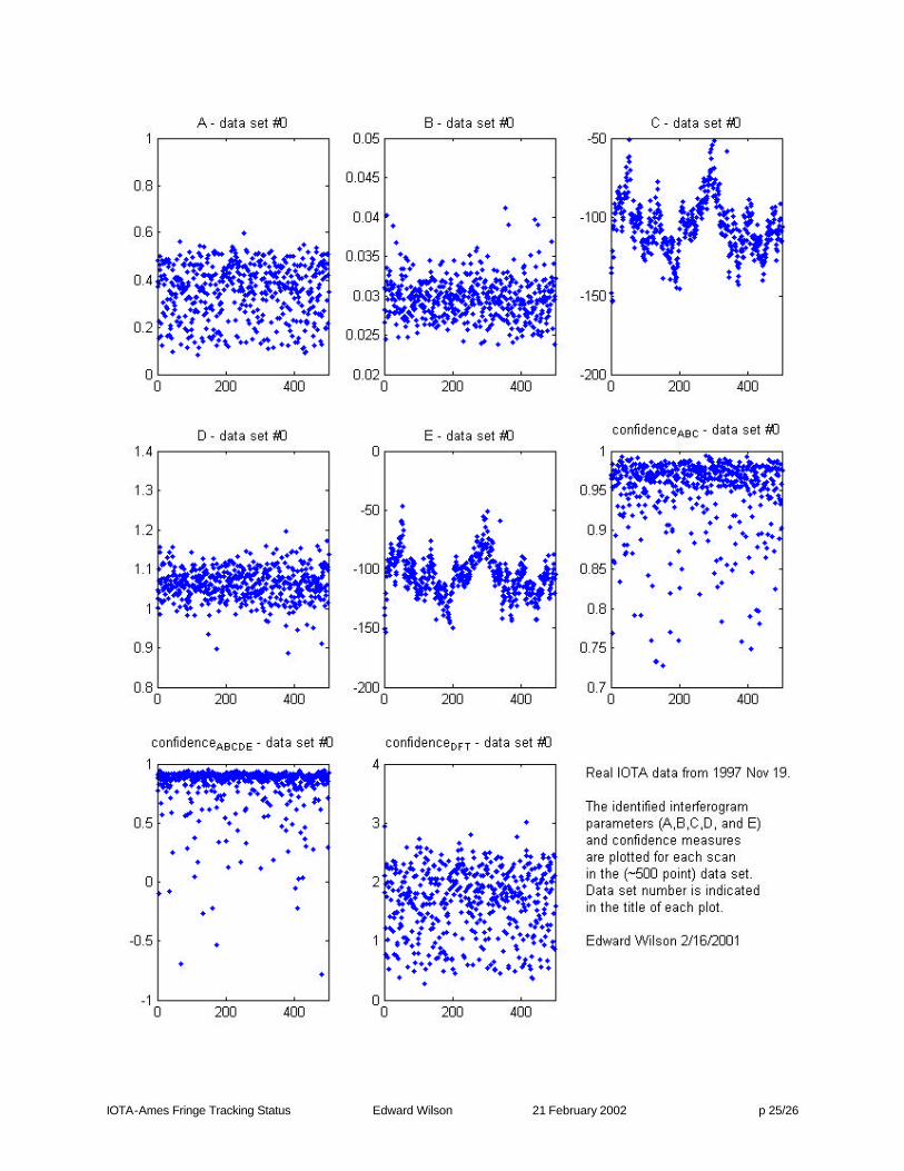
Real IOTA data from 1997 Nov 19. FFT of the identified fringe packet centerposition. A Purely random walk (white, or un-correlated noise) would have a flat spectrum. Atmospheric turbulence theory would predict f(I believe), but f -2/3 seems to be the best fit. Edward Wilson 2/16/2001

FFT of center trajectoryf -4/3 (expected from theory?)f -2/3 (~best fit)


3. Interferogram motion prediction Initial experiments with fringe packet motion prediction were performed. An adaptive linear model was developed as a first step. This model produced approximately 5% (and as high as 10%) improvement over no prediction (i.e., the baseline case of predicting that the fringe packet will remain where it is on the next scan). The next step is to extend the predictive model to a nonlinear neural network. In the data analysis that follows, different sets of parameters from the ideal equation were used, along with the changes in those parameters, to predict the change in interferogram center and the absolute value of the change. A least-squares linear predictor was used for each set of input parameters. The results of each fit were evaluated by testing on a segment of the data that was not used during model development (test data vs. training data). The results of the prediction were tested against a baseline case that: (1) predicted no motion - that the interferogram would stay where it was, and (2) predicted that the absolute value of the motion would equal the RMS of all motion detected so far on that target (this baseline is as good as I could come up with without doing prediction). The percentage improvement from prediction is printed in the following table, which has each of the 9 data sets in rows (there are 8 ~500 point data sets, and the 9th set is all 8 combined), and each of the 8 input parameter combinations tested in columns. col1 col2 col3 col4 col5 col6 col7 col8 | [Mean] Data set 0 7.507 7.854 7.765 6.521 3.889 6.680 4.097 6.489 | 6.350 Data set 2 8.939 9.978 9.550 10.232 6.238 6.826 4.961 6.272 | 7.874 Data set 3 5.267 4.787 4.717 4.959 -0.818 5.280 4.673 2.829 | 3.962 Data set 5 2.312 2.786 3.883 3.583 3.556 3.841 2.804 2.739 | 3.188 Data set 6 7.506 7.581 7.453 7.502 3.026 4.301 6.893 2.850 | 5.889 Data set 7 0.778 -0.149 0.836 1.832 0.637 1.790 2.566 -0.279 | 1.001 Data set 8 -0.102 2.864 3.118 3.067 -0.350 3.017 3.861 2.768 | 2.280 Data set10 0.841 2.403 0.890 0.880 0.511 1.954 0.674 1.270 | 1.178 Data set11 2.940 2.675 3.081 3.074 1.476 2.953 2.931 1.259 | 2.548 --------------------------------------------------------- [Mean] 3.998 4.531 4.588 4.628 2.018 4.071 3.718 2.911 Variables used in prediction [y = A * sinc(B(x+C)) .* cos(D(x+E))]: col 1 : A B C D E A_delta B_delta C_delta D_delta ones_n_1 col 2 : C D B_delta C_delta D_delta ones_n_1 col 3 : C D B_delta C_delta ones_n_1 col 4 : C D C_delta ones_n_1 col 5 : D C_delta ones_n_1 col 6 : C C_delta ones_n_1 col 7 : C D ones_n_1 col 8 : C D C_delta Data sets used: Data set 0 Object: HR#3791.000 Time stamp: 1997 Nov 19 12:00:26 UTC Data set 2 Object: HR#3791.002 Time stamp: 1997 Nov 19 12:24:14 UTC Data set 3 Object: c_HR2188.000 Time stamp: 1997 Nov 19 09:50:40 UTC Data set 5 Object: c_HR8691.000 Time stamp: 1997 Nov 19 03:01:39 UTC Data set 6 Object: c_HR876.000 Time stamp: 1997 Nov 19 07:04:23 UTC Data set 7 Object: t_51_Peg.000 Time stamp: 1997 Nov 19 03:11:09 UTC Data set 8 Object: t_51_Peg.001 Time stamp: 1997 Nov 19 03:23:42 UTC Data set 10 Object: t_51_Peg.003 Time stamp: 1997 Nov 19 04:03:59 UTC Data set 11 Object: IOTA_0_through_10 Time stamp: 1997 Nov 19 03 to 12 UTC


Brief summary of present status:

• Interferogram center ID works very well on the data sets tested so far, including the 1997 data and data generated by a light source using the IOTA configuration as of Feb 2002. The fringe-center estimate provided by the initial steps of the full algorithm (shown in Figures 1-9) appears to be sufficiently accurate for fringe tracking. That is, the initial estimate of C in the equation y = A sinc(B(x+C)) cos(D(x+E)) is sufficient, and full nonlinear estimation of A, B, C, D, E provides only marginal improvement.

• Implementation of this algorithm at IOTA was completed on 2/15/02, and it was successfully

tested on fringes generated by a light source. Compute time on the real-time PowerPC processor is 1.22 ms per scan for one telescope pair. This could be reduced to 0.17 ms with minimal effect on performance if compute time is a major issue.

• Modeling the effect of atmospheric turbulence is in its very early stages. Dawn McIntosh

([email protected]) is leading this effort at the SSRL. We will be very receptive to any guidance from IOTA on this. This will be useful for control system development in simulation.

• Prediction of interferogram motion appears feasible to a small extent, but major effort in this area

is probably not warranted since the payoff appears small relative to that possible through fringe tracking control (without prediction).

Next steps:

• Algorithm tuning – although the algorithm appears to be very robust, some improvements may be required after testing on the sky. We will communicate with Ettore Pedretti to provide any updates as required.

• Publish paper on the results. • Develop neural-network-based nonlinear fringe motion predictor.


Appendix A - 1997 Data We are working with 8 data sets of approximately 500 scans each, with each scan containing 256 points. The data was all taken on 19 Nov 1997 (UTC) with the following time stamp and object name: Number Object name Time stamp

0 HR#3791.000 1997 Nov 19 12:00:26 UTC 2 HR#3791.002 1997 Nov 19 12:24:14 UTC

3 c_HR2188.000 1997 Nov 19 09:50:40 UTC 5 c_HR8691.000 1997 Nov 19 03:01:39 UTC 6 c_HR876.000 1997 Nov 19 07:04:23 UTC

7 t_51_Peg.000 1997 Nov 19 03:11:09 UTC 8 t_51_Peg.001 1997 Nov 19 03:23:42 UTC 10 t_51_Peg.003 1997 Nov 19 04:03:59 UTC

The data was taken with no adjustment of the scan center, other than the smooth mirror drive that accounts for changes in path length due to the rotation of the earth. This was done so the movement of the fringe packet center would be a result of the atmospheric distortion only. Tip-tilt control was functioning. Example raw data plots from both detectors are shown in the following figure.

0 50 100 150 200 25050

100

150

200

250

300

350Raw data from detectors A and B - data set #0, scan #1


Appendix B – Paper published in Proceedings of the 18th Congress of the International Commission for Optics, San Francisco, California, August 1999.

On-line fringe tracking and prediction at IOTA Edward Wilson Robert Mah Intellization Smart Systems Lab, Information Sciences Division 454 Barkentine Lane NASA Ames Research Center Redwood Shores, CA 94065-1126 MS 269-1, Moffett Field, CA 94035 [email protected] [email protected]

Abstract The Infrared/Optical Telescope Array (IOTA) is a multi-aperture Michelson interferometer located on Mt. Hopkins near Tucson, Arizona. To enable viewing of fainter targets, an on-line fringe tracking system is presently under development at NASA Ames Research Center. The system has been developed off-line using actual data from IOTA, and is presently undergoing on-line implementation at IOTA. The system has two parts: (1) a fringe tracking system that identifies the center of a fringe packet by fitting a parametric model to the data; and (2) a fringe packet motion prediction system that uses characteristics of past fringe packets to predict fringe packet motion. Combined, this information will be used to optimize on-line the scanning trajectory, resulting in improved visibility of faint targets. Fringe packet identification is highly accurate and robust (99% of the 4000 fringe packets were identified correctly, the remaining 1% were either out of the scan range or too noisy to be seen) and is performed in 30-90 milliseconds (depending on desired accuracy) on a Pentium II-based computer. Fringe packet prediction, currently performed using an adaptive linear predictor, delivers a 10% improvement over the baseline of predicting no motion. Fringe packet identification To enable on-line tracking and prediction, the first step is to autonomously identify the center of a fringe packet. The approach taken here was to fit the raw data (after some simple filtering) to a parametric model representing a distortion-free fringe packet. The parametric model chosen was:

y = A sinc(B(t+C)) cos(D(t+E)) where y is the normalized value from the interferometer ((channelA-channelB)/(channelA+channelB)), t is time, shown on the horizontal axis on the plot below. This particular grouping of parameters (e.g., D(t+E) instead of Dt + E) was chosen to facilitate gradient-based optimization of the functional parameters. A combination of linear regression, gradient-based optimization, and fast Fourier transform (FFT) tools were used in designing the parameter identification algorithm. The center of the fringe packet is represented by parameter C, and is the only one needed for simple fringe tracking. For prediction of fringe motion (and possible extensions, including on-line data reduction), all 5 parameters are useful. Fringe packet parameters were identified on the 4000-scan data set from IOTA to an accuracy as good as can be determined by eye. That is, we can find fringe packet parameters (amplitude, spread of sinc function, center, frequency of fringes, and phase shift of fringes) that appear to be the “best” match to the actual data. The fringe packet identification algorithm is discussed later. Shown in these figures is an example of fitting to some data from IOTA. The plot on the left shows superposition of y = ±A sinc(B(t+C)) with the actual data (data is discrete - one scan contains 256 points, but points have been connected to improve data visualization). In addition to this, the plot on the right is zoomed in on the packet center and also shows the superposition of the full function, y = A sinc(B(t+C)) cos(D(t+E)).

0 50 100 150 200 250

-0.5

-0.4

-0.3

-0.2

-0.1

0

0.1

0.2

0.3

0.4

0.5

90 95 100 105 110 115 1 2 0 1 2 5 130 135

-0.5

-0.4

-0.3

-0.2

-0.1

0

0.1

0.2

0.3

0.4

0.5


Summary of the steps in identification: 1) Data sets from each of the two collectors are combined: y=(channelA-channelB)/(channelA+channelB) 2) Outliers and local bias are removed 3) The envelope of the absolute value of the signal is calculated, eliminating the individual fringes. Ideally this

function would be y = A abs(sinc(B(t+C))) 4) An estimate for the center of the fringe packet (C) is found by maximizing weighted symmetry over the

envelope. 5) Using an initial guess for B, the rema ining parameter A is found by a least squares fit to the data. 6) Now that A, B, and C have good initial estimates, a gradient-based optimization is performed to find A, B, and

C that form the least squares fit to the data. 7) The fringe parameters, D and E, are found by fitting the ideal fringe function to the data over the center of the

fringe packet (half height of the sinc function determines the center region). 8) An FFT provides an initial guess for D and E, and a gradient-based optimization finds C, D and E, with A and B

held fixed. Simultaneous gradient-based optimization of A, B, C, D, and E was tried, but did not work as well on the noisy data as the sequential procedure listed above. One example of a reason for this difficulty can be seen in the accompanying figure. Half-way through the fringe-packet scan, a sudden phase shift was encountered. If all 5 parameters were adapted simultaneously, the result would be a flat line, with A=0, since the identification would be unable to lock onto the left and right halves of the fringe packet. Squared error would be minimized approximately by a flat line, A = 0. With the present algorithm, two parameters representing the sinc function envelope (A and B) were held fixed while the fringe frequency and phase shift (D and E) were identified. The identification locked onto the right half of the fringe packet since that resulted in a better fit than the left half. Simulation of the effect of atmospheric turbulence on the optical path difference was pursued to enable development of simulated fringe packet data. With simulated data, it will be possible to quantify the accuracy of the fringe packet identification, and possibly refine the identification algorithms. Prediction of fringe-packet-center motion Initial experiments with fringe packet motion prediction were performed. An adaptive linear model using present and past identified fringe parameters was developed as a first step. The center of the next fringe packet and the magnitude of fringe-packet-center motion were predicted, with the goal of optimizing on-line the parameters (e.g., travel limits and rate) of the next scan. This model produced approximately 10% improvement over no prediction (i.e., predicting that the fringe packet would remain where it was on the next scan). Extension to nonlinear prediction methods, including neural networks is under investigation. Summary and future research On-line fringe tracking and identification algorithms have been developed based on off-line data from the IOTA interferometer. Autonomous identification of fringe packet centers, even in the presence of poor signal-to-noise ratio, has been demonstrated using algorithms that can run fast enough to enable real-time implementation (30-90 milliseconds on a Pentium II-based computer). Some encouraging results on fringe-packet motion prediction have been obtained using an adaptive linear predictor. Major areas of future work include implementing these algorithms on the IOTA interferometer (presently underway) and extending the fringe packet prediction algorithm to a nonlinear neural network.


Appendix C: Selected data analysis results – all from the 1997 data set

0 200 40040

60

80

100

120

140

160Center location, data set #0

0 200 40060

80

100

120

140

160


0 200 4000

50

100

150

200


0 200 4000

50

100

150

200


0 200 4000

50

100

150


0 200 4000

50

100

150


0 200 4000

50

100

150

200


0 200 40020

40

60

80

100

120

140


Real IOTA data from 1997 Nov 19. The identified center of the interferogramis plotted for each entire (~500 point) data set, showing the ~random walk and variability in noise characteristics from one data set to the next. Edward Wilson 2/16/2001


0.5 1 1.50

50

100

150

200

250Fringe frequency, data set #0

0.5 1 1.50

100

200

300


0.5 1 1.50

20

40

60

80

100

120


0.5 1 1.50

10

20

30

40

50

60


0.5 1 1.50

50

100

150

200


0.5 1 1.50

10

20

30

40

50

60


0.5 1 1.50

20

40

60


0.5 1 1.50

50

100

150


Real IOTA data from 1997 Nov 19. The identified fringe frequency, D in the ideal equation, y = A * sinc(B(x+C)) .* cos(D(x+E)),is plotted as a histogram. Any values below 0.5 or above 1.5 are not shown. Edward Wilson 2/22/2001


0 100 200-0.4

-0.3

-0.2

-0.1

0

0.1Scan #10, data set #0

0 100 200-0.6

-0.4

-0.2

0

0.2


0 100 200-0.8

-0.6

-0.4

-0.2

0Scan #10, data set #3

0 100 200-0.8

-0.6

-0.4

-0.2

0

0.2

0.4


0 100 200-0.6

-0.4

-0.2

0

0.2


0 100 200-0.4

-0.3

-0.2

-0.1

0

0.1

0.2


0 100 200-0.6

-0.4

-0.2

0

0.2


0 100 200-0.4

-0.3

-0.2

-0.1

0

0.1

0.2


Real IOTA data from 1997 Nov 19. Examples of the raw (combined from the two collectors) data from each data set. The10th scan (arbitrarily chosen) from each data set is plotted. Edward Wilson 2/16/2001


This particular scan represents a problem that was noticed in some other scans as well. It looks like there was a sudden phase shift at around the 102nd data point. This resulted in the overall interferogram envelope to be fit very well (confidenceenvelope = 0.958 where 1.0 is a perfect fit), but the fitting of the fringes as well as the envelope (the entire 5-parameter function) was very bad (confidenceall = -0.004 where 1.0 is a perfect fit). Both confidence measures are normalized RMS error calculations. After visual inspection of the result, the 102nd data point was replicated 3 times, indicated by the blue points in the lower plot (they appear to be at slightly different values due to the pre-filtering that removed the local bias). This resulted in a much better fit of the individual fringes (and increase in confidenceall to 0.803), confirming the sudden phase shift. Could this have been an atmospheric effect, or is it more likely a data collection or mechanical problem in the optics?

80 90 100 110 120 130 140-0.3

-0.2

-0.1

0

0.1

0.2

0.3

0.4confidence

envelope = 0.958

confidenceall

= -0.004

confidenceDFT

= 1.556

Object: HR#3791.002; Time stamp: 1997 Nov 19 12:24:14 UTC; Data set #2; Scan #5

80 90 100 110 120 130 140-0.3

-0.2

-0.1

0

0.1

0.2

0.3

0.4confidence

envelope = 0.950

confidenceall

= 0.803

confidenceDFT

= 1.134

Object: HR#3791.002; Time stamp: 1997 Nov 19 12:24:14 UTC; Data set #2; Scan #5

fringe tracking status - harvard university

Documents