From Correlation to Granger Causality

David I. Stern

Crawford School of Economics and Government, Australian National University, Canberra,

ACT 0200, Australia. E-mail: david.stern@anu.edu.au

22nd September 2011

Abstract: The paper focuses on establishing causation in regression analysis in observational

settings. Simple static regression analysis cannot establish causality in the absence of a priori

theory on possible causal mechanisms or controlled and randomized experiments. However,

two regression based econometric techniques – instrumental variables and Granger causality -

can be used to test for causality given some assumptions. The Granger causality technique is

applied to a time series data set on energy and economic growth from Sweden spanning 150

years to determine whether increases in energy use and energy quality have driven economic

growth. I show that the Granger causality technique is very sensitive to variable definition,

choice of additional variables in the model, and sample periods. Better results can be

obtained by using multivariate models, defining variables to better reflect their theoretical

definition, and by using larger samples. The better specified models with larger samples are

more likely to show that energy causes output growth but it is also possible that the

relationship between energy and growth has changed over time. Energy prices have a

significant causal impact on both energy use and output while there is no strong evidence that

energy use causes carbon and sulfur emissions despite the obvious physical relationship. It is

likely that instrumental variable techniques also are subject to similar vagaries of

specification.

Acknowledgements: I thank Paul Burke and Md. Shahiduzzaman for very useful comments.

Introduction

The dictum “correlation does not imply causation” is so well known that it has its own

Wikipedia page. Yet this does not stop untold numbers of social scientific studies from

making causal claims based on simple regression analysis of non-experimental data with

weak or no analysis of possible causal mechanisms. With no additional information,

regression analysis can only be used to estimate the partial correlations between variables.

Causal inferences can be made from non-experimental data using standard regression

analysis but the process is not straightforward (Freedman, 2007). Researchers must use

theory to establish potential causal mechanisms (Heckman, 2008), determine if variables are

truly exogenous, and ensure that there are no confounding omitted variables. There are,

however, some more sophisticated regression-based techniques – instrumental variables and

Granger causality tests – that can be used to test for causality under weaker conditions,

though some assumptions are still needed. In this paper, I review these techniques and the

potential issues in using them and illustrate the approach by applying Granger causality

testing to modeling the relationship between energy use and economic growth.

To keep things simple, in this section of the paper I examine a model with a single dependent

variable and several explanatory variables. This is extended to true multivariate models in the

following section of the paper. As is well-known, ordinary least squares (OLS) is the best

linear unbiased estimator (BLUE) of the regression parameter vector β in the following

regression model:

€

y = Xβ + ε (1)

where y is the vector of observations on the dependent variable, X is the matrix of

observations on the explanatory variables, and ε the vector of errors if:

E[ε] = 0 (2)

Cov(X,ε) = 0 (3)

E[εε'] = σ2I (4)

and that the matrix X has full column rank (Greene, 1993). In words, it is assumed that the

error term has mean zero, is homoskedastic, and has no serial correlation, that there is no

correlation between the regressors and the errors, and that there are no exact linear

relationships between the regressors. The OLS estimator of β is given by

€

ˆ β OLS = X 'X( )−1X ' y .

It is usual to assume that the error terms are also normally distributed, in which case OLS is

the maximum likelihood estimator. OLS is still an unbiased estimator if (4) does not hold as

long as the other assumptions do and the error term is stationary if serially correlated.1

The main enemies or barriers to establishing causal relations are endogeneity and omitted

variables.2 By endogeneity I mean that there is reverse causation from the dependent variable

to one or more of the explanatory variables.3 In the classic regression model both lead to a

correlation between the regressors and the error term violating (3) and resulting in biased

estimates. More straightforwardly they mean in the former case that the direction of causality

may not be clear and in the second that though there could be a correlation it might simply be

due to a third omitted variable that influences both the explanatory and dependent variable.

If instead the classical regression conditions hold true then we can give the regression

equation a causal interpretation. The explanatory variables will be exogenous – not caused by

the dependent variable y – and there will be no omitted variables correlated with the

explanatory variables. Measurement error in the explanatory variables can also cause the

                                                                                                               

1  Note, that in the time series case it is not necessary that the variables are stationary, it is the error term that has to be stationary. In the case of variables with linear time trends and stationary stochastic components it is easy to generate spurious regressions by regressing unrelated but trending variables on each other. Regressions may seem extremely significant. The explanation is that this is a case of omitted variables bias. Other linearly trending variables that are the true explanatory variables for the dependent variable have been omitted from the regression. These trending variables are correlated with the included irrelevant variable, which acts as a proxy. This correlation can be removed by either detrending all the variables first, or by equivalently including a trend variable in the regression. Yule (1926) showed that nonsense correlations are also likely to arise between short segments of highly serially correlated series, which are in fact stationary in large enough samples.

2  Measurement error will also bias the estimated coefficients and non-spherical errors will affect the efficiency of estimation and significance testing. These may affect the estimated strength of the relationship but are unlikely to produce totally spurious results. Another very important issue is small sample sizes, which result in low statistical power and hence difficulty in determining if there are any real relationships among the variables. This point is taken up again in the discussion of the energy and growth literature.  3 Endogeneity is often used in a broader sense (Deaton, 2010). Wooldridge (2009, 838) defines an endogenous variable as one “that is correlated with the error term, either because of an omitted variable, measurement error, or simultaneity.” I am using the term “endogeneity” to refer to what Wooldridge calls “simultaneity”.

violation of (3) but will not cause us to believe there is a relationship where none exists –

usually the opposite is the case (Hausman, 2001).

The problem is that (3) cannot generally be directly tested statistically. This condition is

effectively imposed when computing the regression coefficients. It can only be determined if

it is valid using additional information. However, misspecification tests can point to omitted

variables issues. For example, Hausman (1978) misspecification tests can be used to test for

omitted variables in panel data models. If the test finds that the parameter estimates of the

fixed effects and random effects estimates differ, it is probably because there are omitted

variables that are correlated with the individual effect. The Hausman test can also be used to

test for measurement error by comparing the coefficients estimated by OLS with an

alternative instrumental variables estimator (Greene, 1993).4 Cointegration analysis of non-

stationary time series data can also be used to suggest that stochastically trending variables

have been omitted.

In some instances exogeneity and causality are obvious. For example, in a joke paper,

Bezimeni (2011) claims 5 to regress individual ages from survey data on responses to a

survey question on trust a factor derived from a factor analysis of various variables and the

percentage of overqualified women in national parliaments’ cafeterias. Clearly, individual

age is exogenous and cannot be caused by any of the explanatory variables. Therefore, the

supposed regression is nonsense. Instead, age might explain some of the responses. But

average age in a location might be an endogenous variable and researchers need to be

cautious of using it as an explanatory variable in a regression. For example, if we regressed

income per capita in local government areas in Australia on average age, we could not

necessarily interpret the results causally, as the age composition of a location will depend to

some degree on the economic opportunities available and vice versa.

Then there are cases where an explanatory variable is clearly exogenous and appears to have

a significant effect on the dependent variable and yet theory suggests that the relationship is

spurious and due to omitted variables that happen to be correlated with the explanatory

                                                                                                               4 Of course, this requires us to construct a valid instrumental variables estimator, which could be difficult.

5  Though regression results are reported, it is obvious from the variables named that no regression analysis was in fact conducted.  

variable in question. Westling (2011) regresses national economic growth rates on average

reported penis lengths and other variables and finds that there is an inverted U shape

relationship between economic growth and penis length from 1960 to 1985. The growth

maximizing length was 13.5cm, whereas the global average was 14.5cm. Penis length would

seem to be exogenous but the nature of this relationship would have changed over time as the

fastest growing region has changed from Europe and its Western Offshoots to Asia.6 So, it

seems that the result is likely due to omitted variables bias.

Establishing Causal Relationships

Instrumental Variables

If relevant variables are omitted from the matrix X in the regression model (1) that are

correlated with the included variables or any of the included explanatory variables are caused

at least partially by the dependent variable y, then the covariance between X and the true error

term ε will be non-zero. In the former case, the error term includes all the relevant factors

needed to explain the variation in y that have been omitted from the model, so if any of these

are correlated with the included variables the included variables will be correlated with the

error term. In the latter case, the dependent variable is a function of the explanatory variables

and the error term. So if any of the explanatory variables are in fact driven by the dependent

variable they will be a function of the error term and hence correlated with it. As mentioned

above, errors in measuring the explanatory variables, X, can also result in Cov(X,ε) being

non-zero.

The method of instrumental variables (IV) introduces a new variable or set of variables Z that

meets the following conditions:

i. Z is correlated with X.

ii. Cov(Z,ε) = 0

iii. Z only affects y through X and can be excluded from the regression equation (1).

Then the IV estimator of estimator of β is given by

€

ˆ β IV = Z 'X( )−1Z ' y . The estimator is biased

but consistent. The IV estimator can also be interpreted as performing a two-stage regression

procedure. First, X is regressed on the instrumental variables Z. Then the predictors of X from                                                                                                                

6  According to Westling’s data, penis length is lowest in Asia and greatest in Africa with Europe and its Western Offshoots having intermediate lengths.  

this first stage regression are used in place of the true X in the regression equation (1).7 As Z

is not correlated with the error term the predictor of X from the first stage regression is also

not correlated with the error term and the classic regression conditions listed above are met.

Given this, the regression coefficients can be given a causal interpretation. The main

difficulty in implementing the IV approach is in finding appropriate instrumental variables.

The classic case of problems due to endogeneity of the explanatory variables is the

simultaneous equations model. For example a model of supply and demand where both price

and quantity are endogenous. For example, the quantity demanded in the market as a whole is

a function of the market price and other variables.8 But market price is determined by

equilibrium between supply and demand and hence is endogenous in the demand equation.

The instrumental variables approach looks for variables that affect the price that suppliers

will charge that will not affect the quantity demanded directly. For example in an agricultural

crop model the weather in the growing regions would be expected to affect supply but not

demand directly. But it is not always possible to find such plausible examples of variables

that would qualify as instruments particularly when we are dealing with macro-economic

models. In order to identify each equation at least one exogenous variable must be excluded

from each equation for each endogenous variable included. As the number of endogenous

variables increases it gets harder to justify the large number of restrictions needed. In the

context of macro-economic models, Sims (1980) referred to these as incredible or even

spurious restrictions.

Recently, the instrumental variables technique has been popularized (Angrist and Pischke,

2008; Levitt and Dubner, 2005) as a method for dealing with omitted variables bias

particularly in the context of policy evaluation (Angrist and Krueger, 2001). For example, we

might want to estimate the effect of additional schooling on earnings. But we cannot observe

underlying ability, which might determine both the amount of schooling that students decide

to undergo and their future earnings too. If we could randomly force some students to stay in

school longer and some to stay in school for less time, the correlation of schooling with

                                                                                                               

7  Implementing this two-step procedure manually with a standard regression package will not, however, generate the correct standard errors for the estimated regression parameters. Therefore, it advisable not to use this approach in practice.  

8  Note that if we are modeling the quantity demanded by individuals the market price could be taken as exogenous, assuming a single market price.  

ability would disappear. But this sort of randomized experiment is rarely, if at all, possible. If

we can find an instrumental variable that is correlated with schooling but not with ability and

which should not directly affect earnings either then we can use the IV approach to obtain a

causal estimate of the effect of schooling on earnings. But finding such a variable is not

straightforward. Angrist and Krueger (1991) exploited the fact that in most US states students

started their school career at the beginning of a school year but could end it as soon as they

hit their 16th birthday. This meant, that children who quit school on their 16th birthday were

forced to attend school for different lengths of time, with children born earlier in the school

year attending school for less time. They argued, therefore, that date of birth was a valid

instrument for schooling, at least from 1930 to 1959 in the United States. As a result they

estimated that an additional year of schooling increased income by 10%. Angrist and Krueger

(2001) point out, however, that their estimate only depends on the choices of those who drop

out of school on their 16th birthday. It is possible that those that continue their schooling

further have a different return to schooling than those that drop out. Whereas the length of

schooling is assigned randomly the act of dropping out is not. They term this a Local Average

Treatment Effect or LATE. Dunning (2008) discusses a related issue - the assumption of

homogenous causal effects across portions of the endogenous regressor. For example, if

lottery winnings are used as an instrument for income in a model of the effect of income on

political beliefs, it is assumed that lottery income and non-lottery income have the same

effect on people’s political beliefs. But this might not be true.

Invalid instruments are correlated with the error term and can cause the results to be even

worse than OLS results (Hahn and Hausman, 2003). Instrument validity can only be tested in

an over-identified model where the number of instruments is greater than the number of

endogenous variables. The Sargan (1958) test is used most frequently.

Another practical issue that arises in implementing the IV method is the problem of “weak

instruments” – instrumental variables that are not in fact strongly correlated with the model

explanatory variables and in the case of measurement error when the size of the measurement

error is large (Hausman, 2001). The weak instrument may simply be uninformative but the

usual estimated standard errors may not reflect this (Imbens and Rosenbaum, 2005) and the

estimate tends to be biased towards the OLS estimates (Angrist and Krueger, 2001; Hausman

and Hahn, 2003). Hausman and Hahn (2003), Imbens and Rosenbaum (2005), and Stock and

Yogo (2005) provide a discussion, diagnostics, and potential solutions. Angrist and Krueger’s

(1991) date of birth instrument has been criticized as a weak instrument (Bound et al., 1995).

Bound et al. used a constructed random variable in place of Angrist and Krueger’s (1991)

instrument and obtained similar results to Angrist and Krueger’s IV estimates when they

average over 500 realizations.

Angrist and Pischke (2010) explain that the increased use of IV and experimental techniques

was a response to Leamer’s (1983) critique of the micro-econometric practice of the time.

Leamer argued that most econometric results were not robust because the necessary

conditions for a causal interpretation of regression were not met. A decade later, Levine and

Renelt (1992) provided similar evidence for cross-sectional macro-econometrics. They found

that very few macroeconomic variables used in econometric studies of growth were robustly

correlated with cross-country growth rates. This situation does not seem to have improved

with time (Eberhardt and Teal, 2011). In a critique discussed in more detail below, Sims

(1980) argued that time series macro-econometrics also suffered from “incredible”

identifying restrictions.

There has been considerable recent controversy around the use of instrumental variable

techniques (e.g. Angrist and Pischke, 2010; Heckman, 2010; Heckman and Urzua, 2010;

Keene, 2010a; Sims, 2010; Deaton, 2010; Imbens, 2010). This appears to stem from the

exaggerated claims of Angrist and co-researchers that his approach had made econometric

results credible to economists and policy-makers in a way that structural models never could

(e.g. Angrist and Pischke, 2010). Angrist’s approach is seen as an “atheoretical” approach to

econometrics (Keane, 2010b), whereas this section has discussed IV techniques much more

broadly, so this critique does not apply to all IV approaches. In fact, the structural models

promoted by Heckman and Keane will often use IV estimation. In reality, Angrist’s approach

is just one tool in the econometrics toolbox. Keane (2010a) admits that “the experimentalist

school has done a great service to empirical economics by forcing researchers to pay more

attention to the sources of variation in data that identify their models” (53). In the past, not

much attention was frequently given to whether instrumental variables in simultaneous

equation models were legitimate. That is less the case today. But this does not mean that

other approaches to econometrics, done properly, are not credible as Angrist and Pischke

(2010) seem to claim.

Granger Causality Testing

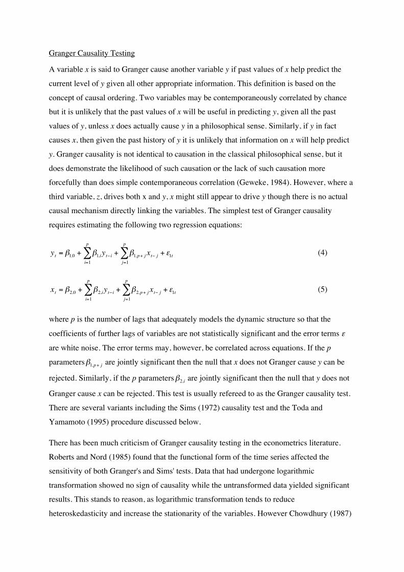
A variable x is said to Granger cause another variable y if past values of x help predict the

current level of y given all other appropriate information. This definition is based on the

concept of causal ordering. Two variables may be contemporaneously correlated by chance

but it is unlikely that the past values of x will be useful in predicting y, given all the past

values of y, unless x does actually cause y in a philosophical sense. Similarly, if y in fact

causes x, then given the past history of y it is unlikely that information on x will help predict

y. Granger causality is not identical to causation in the classical philosophical sense, but it

does demonstrate the likelihood of such causation or the lack of such causation more

forcefully than does simple contemporaneous correlation (Geweke, 1984). However, where a

third variable, z, drives both x and y, x might still appear to drive y though there is no actual

causal mechanism directly linking the variables. The simplest test of Granger causality

requires estimating the following two regression equations:

€

yt = β1,0 + β1,ii=1

p

∑ yt− i + β1,p+ jj=1

p

∑ xt− j + ε1t (4)

€

xt = β2,0 + β2,ii=1

p

∑ yt− i + β2,p+ jj=1

p

∑ xt− j + ε1t (5)

where p is the number of lags that adequately models the dynamic structure so that the

coefficients of further lags of variables are not statistically significant and the error terms ε

are white noise. The error terms may, however, be correlated across equations. If the p

parameters

€

β1,p+ j are jointly significant then the null that x does not Granger cause y can be

rejected. Similarly, if the p parameters

€

β2,i are jointly significant then the null that y does not

Granger cause x can be rejected. This test is usually refereed to as the Granger causality test.

There are several variants including the Sims (1972) causality test and the Toda and

Yamamoto (1995) procedure discussed below.

There has been much criticism of Granger causality testing in the econometrics literature.

Roberts and Nord (1985) found that the functional form of the time series affected the

sensitivity of both Granger's and Sims' tests. Data that had undergone logarithmic

transformation showed no sign of causality while the untransformed data yielded significant

results. This stands to reason, as logarithmic transformation tends to reduce

heteroskedasticity and increase the stationarity of the variables. However Chowdhury (1987)

found more disturbing results that give support to those who have doubted whether Granger

causality was related to philosophical causality or economic exogeneity in any meaningful

way. He found that a Granger test indicated that GNP caused sunspots! A Sims test showed

that prices caused sunspots! None of the alternative hypotheses were validated. Prices and

income may be exogenous in the sunspot equations, but sunspots are not endogenous in any

meaningful philosophical or economic way. But because sunspots are quite predictable prices

and income might have anticipated them. The forward-looking behavior of human agents can

be an obstacle to Granger causality testing.

Sargent (1979) and Sims (1980) introduced the vector autoregression or VAR modeling

approach as a method of carrying out econometric analysis with a minimum of a priori

assumptions about economic theory (Qin, 2011). The VAR model generalizes the model

given by equations (4) and (5) to a multivariate setting. A multivariate Granger causality test

can be identical to that described above but simply with more control variables in the

regression but tests can also be constructed to exclude the lags of variables from multiple

equations (Sims, 1980). The VAR approach to econometrics has been much criticized, but

the critics, such as Epstein (1987) and Darnell and Evans (1990), argue that multivariate

Granger causality tests are a (or the only) useful application of VARs. The advantage of

multivariate Granger tests over bivariate Granger tests is that they can help avoid spurious

correlations and can aid in testing the general validity of the causation test. This is through

adding additional variables that may be responsible for causing y or whose effects might

obscure the effect of x on y (Lütkepohl, 1982; Stern, 1993). There may also be indirect

channels of causation from x to y, which VAR modeling could uncover.

Though a VAR cannot, due to limits on degrees of freedom, include all variables that may be

causally related to the principal variable under investigation, some attempt can be made to

include as many as possible. Of course, failure to reject the null hypothesis that x does not

cause y, does not necessarily mean that there is in fact no causality. A lack of sensitivity

could be due to a misspecified lag length, insufficiently frequent observations, too small a

sample, or the lack of Granger causality even if philosophical causation occurs.

Engle and Granger (1987) introduced the notion of cointegration and tied it closely to the

VAR model. Time series that must be differenced in order to render them stationary are

referred to as integrated or stochastically trending series. The simplest case is the classic

random walk where the current value of a variable is equal to its previous value plus a white

noise error term. Typically, linear combinations of integrated process also are integrated.

The residual from a regression of the two variables will be non-stationary. This violates the

classical conditions for a linear regression. Such a regression is known as a spurious

regression (Granger and Newbold, 1974). However, if a group of integrated variables share a

common stochastic trend the linear combination will be non-integrated. This phenomenon -

the elimination of a stochastic trend by an appropriate linear function - is known as

cointegration (Engle and Granger, 1987). If two variables share a common trend, there will

be Granger causality in one or more directions between them (Cuthbertson et al., 1992).

Cointegration tests themselves cannot establish the direction of causality but tests can be

applied to cointegrating VARs such as those estimated using the Johansen procedure

(Johansen and Juselius, 1990). Hendry and Juselius (2000, 2001) provide a good introduction

to cointegration analysis for energy economics.

An advantage of cointegration analysis is that if any integrated variables are omitted from the

cointegrating relationship, which should be included in it, then the remaining variables will

fail to cointegrate. Thus, if we can reject the null of non-causality in a cointegrated model, we

can be more confident that this is not a spurious causality due to omitted variables.

It is now understood that in the absence of cointegration between the variables a Granger

causality test on a VAR in levels is invalid. Ohanian (1988) and Toda and Phillips (1993)

showed that the distribution of the test statistic for Granger causality in a VAR with non-

stationary variables is not the standard chi-square distribution. This means that the

significance levels reported in the early studies of the Granger-causality relationship between

energy and GDP may be incorrect, as both variables are generally integrated series. If there is

no cointegration between the variables then the causality test should be carried out on a VAR

in differenced data, while if there is cointegration, standard chi-square distributions apply

when the cointegrating restrictions are imposed (Toda and Yamamoto, 1995). Toda and

Yamamoto (1995) developed a modification of the standard Granger causality test on the

variables in levels that is robust to the presence of unit roots. But it is still, of course, subject

to possible omitted variables bias. Cointegration tests can be used to test for omitted non-

stationary variables. A lack of cointegration implies that variables essential to cointegration

are omitted from the model. Therefore, testing for cointegration is still a necessary

prerequisite to causality testing on data with potential unit roots.

Thus the notion of Granger causality can be tested by a variety of means depending on the

nature of the data and model. In the remainder of this paper I apply the Toda and Yamamoto

(1995) procedure for Granger causality testing and a version of Engle and Granger’s (1987)

cointegration procedure to the Swedish energy and growth case study to illustrate the

approach.

Energy and Growth: Correlation or Causation?

Background

Does growth in energy availability and use cause economic growth? Or does economic

growth drive increasing energy consumption? The answers to these questions are important

for both understanding economic history and for analyzing energy policies in the area of

climate change, peak oil, energy security etc.

Granger causality and cointegration methods have been extensively used to test for causal

relations between time series of energy, GDP (output), and other variables from the late

1970’s on (Kraft and Kraft, 1978; Ozturk, 2010) and there is now a very large literature.

Early studies relied on Granger causality tests on unrestricted vector autoregressions (VAR)

in levels of the variables, while more recent studies use cointegration methods. The key

variables are likely to be non-stationary and stochastically trending and hence whether the

variables cointegrate is a key issue. Another key characteristic that distinguishes between

studies is whether a bivariate model of energy and output or a multivariate framework is

used. A third way to differentiate among models is whether energy is measured in standard

heat units or whether some type of indexing method is used to account for differences in

quality among fuels.

The results of the early studies that tested for Granger causality using a bivariate model were

generally inconclusive (Stern, 1993). Where nominally significant results were obtained, they

mostly indicated that causality runs from output to energy. However, in many cases results

differed depending on the samples used, the countries investigated etc. Most economists

believe that capital, labor, and technical change play a significant role in determining output,

yet early studies used only energy as an independent variable. Omitted variables bias, non-

cointegration in the case of stochastically trending variables and spurious regression result.

Results are frequently sample dependent in the face of omitted variables and non-

cointegration (e.g. Stern and Common, 2001). This may explain the very divergent nature of

the early causality literature.

Stern (1993) tested for Granger causality in a multivariate setting using a VAR model of

GDP, capital and labor inputs, and a Divisia index of quality-adjusted energy use in place of

gross energy use. The multivariate methodology is important because reductions in energy

use are frequently countered by the substitution of other factors of production for energy and

vice versa, resulting in an insignificant overall impact of energy on output. When both the

multivariate approach and a quality adjusted energy index were employed, energy was found

to Granger cause GDP.

In similar fashion, Hamilton (1983) and Burbridge and Harrison (1984) found that changes in

oil prices Granger-cause changes in GNP and unemployment in VAR models whereas oil

prices are exogenous to the system. More recently, Blanchard and Gali (2008) used VAR

models of GDP, oil prices, wages, and two other price indices, to argue that the effect of oil

price shocks has reduced over time. Hamilton (2009) deconstructs their arguments to show

that past recessions would have been mild or have merely been slowdowns if oil prices had

not risen. Furthermore, he argues that the large increase in the price of oil that climaxed in

2008 was a major factor in causing the 2008-2009 recession. However, as the short-run

elasticity of demand for oil and other forms of energy is low, the main short-run effects of oil

prices are expected to be through reducing spending by consumers and firms on other goods,

services, and inputs rather than through reducing the input of energy to production (Hamilton,

2009; Edelstein and Killian, 2009). Therefore, models using oil prices in place of energy

quantities may not provide much evidence regarding the effects of energy use itself on

economic growth.

Yu and Jin (1992) conducted the first cointegration study of the energy-GDP relationship.

Again, the results of this and subsequent studies differ according to the regions, time frames,

and measures of inputs and outputs used. When multivariate cointegration methods are used,

a picture emerges of energy playing a central role in determining output in a diverse set of

developed and developing nations. Stern (2000) estimated a dynamic cointegration model for

GDP, quality weighted energy, labor, and capital, using the Johansen methodology. The

analysis showed that there is a cointegrating relation between the four variables and that

energy Granger causes GDP either unidirectionally or possibly through a mutually causative

relationship depending on which version of the model is used. Warr and Ayres (2010)

replicate this model for the U.S. using their measures of exergy and useful work in place of

Stern’s Divisia index of energy use. They find both short- and long-run causality from either

exergy or useful work to GDP but not vice versa. Oh and Lee (2004) and Ghali and El-Sakka

(2004) apply Stern’s (1993, 2000) methodology to Korea and Canada, respectively, coming

to exactly the same conclusions, extending the validity of Stern’s results beyond the United

States. Lee and Chang (2008) and Lee et al. (2008) use panel data cointegration methods to

examine the relationship between energy, GDP, and capital in 16 Asian and 22 OECD

countries over a three and four decade period respectively. Lee and Chang (2008) find a long-

run causal relationship from energy to GDP in the group of Asian countries while Lee et al.

(2008) find a bi-directional relationship in the OECD sample. Taken together, this body of

work suggests that the inconclusive results of earlier work are probably due to the omission

of non-energy inputs.

However, using a panel VECM model of GDP, energy use and energy prices for 26 OECD

countries (1978-2005), Costantini and Martini (2010) find that in the short-run energy prices

cause GDP and energy use and energy use and GDP are mutually causative. However, in the

long run they find that GDP growth drives energy use and energy prices. Other researchers

who model a cointegrating relation between GDP, energy, and energy prices for individual

countries produce mixed results. For example, Glasure (2002) finds very similar results to

Costantini and Martini (2010) for Korea, while Masih and Masih (1997) and Hondroyiannis

et al. (2002) find mutual causation in the long-run for Korea and Taiwan and Greece

respectively. Using an idea from meta-analysis (Stanley and Doucouliagos, 2010), we should

probably put most weight on the largest sample study – i.e. Costantini and Martini (2010) -

concluding that these models identify a demand function relationship where in the long run

GDP growth drives energy use.

Chontanawat et al. (2008) test for causality between energy and GDP only using a consistent

data set and methodology for over 100 countries. Causality from energy to GDP is found to

be more prevalent in the developed OECD countries compared to the developing non-OECD

countries. But it is hard to interpret this given the simple bivariate model employed.

Joyeux and Ripple (2011) analyze the cointegrating and causal relations between income and

three energy consumption series - residential electricity consumption, total electricity

consumption, and total energy consumption - based on panel data and the latest panel

methodologies for 30 OECD and 26 non-OECD countries. The results support a finding of

causality flowing from income to energy consumption for developed and developing

economies, alike. Again, this is a simple bivariate analysis.

Until 2010 all papers in this literature examined time series of a few decades at most using

annual data, which is a small sample size for time series analysis though researchers have

used panel data to try to increase statistical power through larger samples. In addition to the

problems of model specification discussed above, small sample sizes might be a reason for

the inconclusiveness of research in this field. Vaona (2010) tests for causality between

Malanima’s (2006) Italian energy data for 1861-2000 and GDP using the Toda and

Yamamoto (1995) procedure and the Johansen cointegration tests. Not surprisingly, given

that the model is bivariate, the latter fail to reject the null of non-cointegration so he also tests

Granger causality in a VAR of first differences. Both models find mutual causation between

non-renewable energy and GDP and from one measure of renewable energy to GDP.

Oxley and Greasley (1998) test for the causes of the industrial revolution in Britain using

Granger causality tests but the variables they consider do not include energy. Stern and

Kander (2011) estimate a model using 150 years of energy, gross output, labor, and capital

data for Sweden. The model has two equations – a nonlinear constant elasticity of

substitution production function for the log of gross output and an equation for the log of the

ratio of energy costs to non-energy costs. Two specifications are estimated – one assumes

that the rate of technological change was constant over the 150-year period and the other

allows the rate to differ in each 50-year period. Using non-linear and linear cointegration tests

they find that the latter model cointegrates but the former does not. This implies that there is

a causal relationship between the variables, but the direction is unknown.

Data and Methods

Data is identical to that compiled by Stern and Kander (2011) where a full description can be

found. The energy data comes from the Kander (2002) and the other data from the Swedish

historical national accounts (Krantz and Schön, 2007).

First we test the series for unit roots using the Phillips and Perron (1988, PP) test, which has a

null of unit root and the Kwiatowski et al (1992, KPSS) test which has a null of stationarity.

All variables are transformed into logarithms before testing. The variables considered are:

Gross output (GRO), GDP (GDP), Capital (K), Labor (L), Heat content of primary energy

(HE), Divisia index of primary energy (DE), Energy price index deflated by the GDP deflator

(PE), Oil price deflated by the GDP deflator (PO).

The reason for looking at the price of oil is that it is more exogenous than the energy price

index but the series only starts in 1885. I carry out tests for the full 150 year period and for

each individual 50 year period as well as Stern and Kander (2011) found cointegration when

they allowed technical change to be constant for 50 years but not for 150 years. In order to

determine the order of integration I test both the levels and the first differences of the

variables. The PP testing procedure follows that in Stern (2000) exactly based on Enders

(1995) who gives critical values. The regression model that the test is based on is as follows:

€

Δyt =α + βt + γyt−1 + εt (6)

This full model is designated Model 1. The model without the time trend is designated Model

2 and without the constant as well Model 3. Tests on these models are more powerful because

of the absence of extraneous parameters. We use the default four lags to compute the Newey-

West standard errors used by the RATS procedure unitroot.src.

I estimate a variety of VAR models to test some of the various ideas in the literature. These

include bivariate and multivariate models and are discussed in the results section. I initially

tested for the optimal VAR lag length using the likelihood ratio test (Sims, 1980) with four

lags being the maximum considered according to the Schwert (1989) criterion and a 10%

significance level. But results seemed quite sensitive in some cases to the number of lags

when these were only one or two and I decided to estimate each model with four lags plus an

additional two lags, which is equal to the maximum order of integration of the variables.

Adding too many lags results in lowered efficiency of estimation but using too few results in

bias. So it is better to err on the high side.  Causality is tested by excluding only the first four

lags. This is the Toda and Yamamoto (1995) procedure for testing for causality in the

possible presence of unit roots and non-cointegration.

I also estimate a vector error-correction model (VECM), which is a VAR that imposes

cointegration restrictions:

€

Δyt =α + ΒiΔyt− ii=1

p

∑ + Γet− i + εt (7)

where y is the vector of variables, ε the vector of error terms, and e a vector of error

correction terms. The dimension of e is less than that of y. B and Γ are matrices of regression

parameters. The Engle-Granger approach first estimates a cointegrating regression using

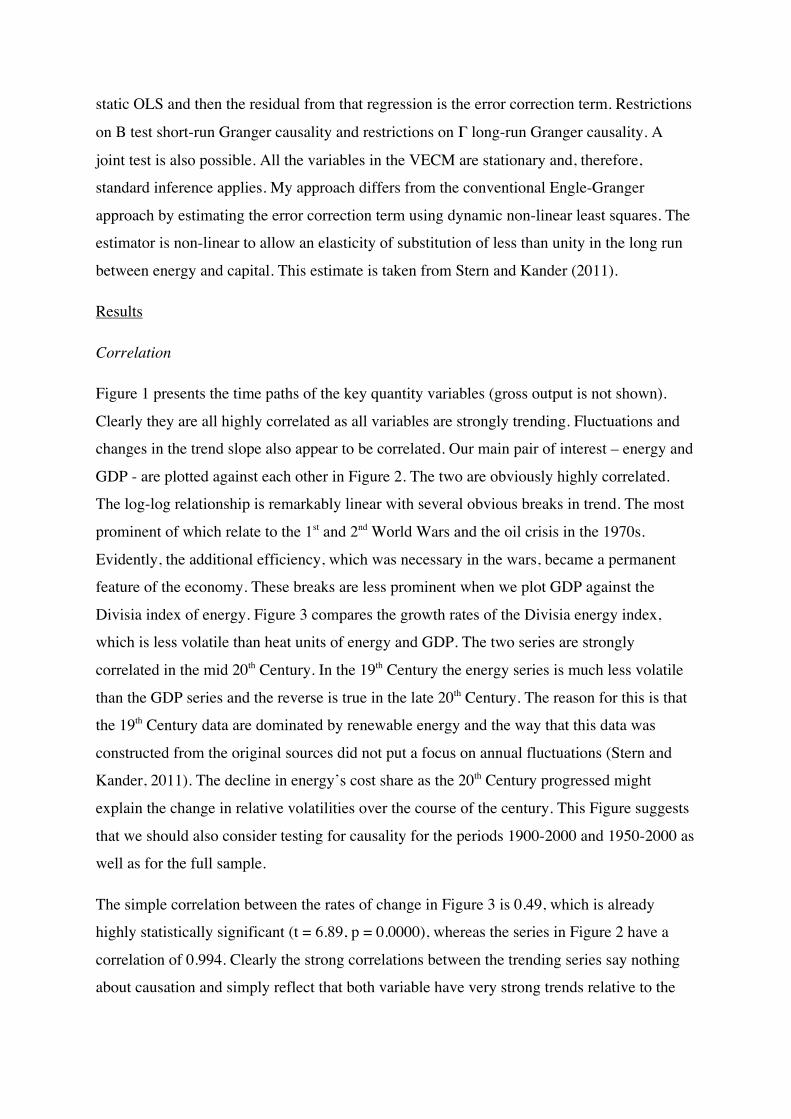
static OLS and then the residual from that regression is the error correction term. Restrictions

on B test short-run Granger causality and restrictions on Γ long-run Granger causality. A

joint test is also possible. All the variables in the VECM are stationary and, therefore,

standard inference applies. My approach differs from the conventional Engle-Granger

approach by estimating the error correction term using dynamic non-linear least squares. The

estimator is non-linear to allow an elasticity of substitution of less than unity in the long run

between energy and capital. This estimate is taken from Stern and Kander (2011).

Results

Correlation

Figure 1 presents the time paths of the key quantity variables (gross output is not shown).

Clearly they are all highly correlated as all variables are strongly trending. Fluctuations and

changes in the trend slope also appear to be correlated. Our main pair of interest – energy and

GDP - are plotted against each other in Figure 2. The two are obviously highly correlated.

The log-log relationship is remarkably linear with several obvious breaks in trend. The most

prominent of which relate to the 1st and 2nd World Wars and the oil crisis in the 1970s.

Evidently, the additional efficiency, which was necessary in the wars, became a permanent

feature of the economy. These breaks are less prominent when we plot GDP against the

Divisia index of energy. Figure 3 compares the growth rates of the Divisia energy index,

which is less volatile than heat units of energy and GDP. The two series are strongly

correlated in the mid 20th Century. In the 19th Century the energy series is much less volatile

than the GDP series and the reverse is true in the late 20th Century. The reason for this is that

the 19th Century data are dominated by renewable energy and the way that this data was

constructed from the original sources did not put a focus on annual fluctuations (Stern and

Kander, 2011). The decline in energy’s cost share as the 20th Century progressed might

explain the change in relative volatilities over the course of the century. This Figure suggests

that we should also consider testing for causality for the periods 1900-2000 and 1950-2000 as

well as for the full sample.

The simple correlation between the rates of change in Figure 3 is 0.49, which is already

highly statistically significant (t = 6.89, p = 0.0000), whereas the series in Figure 2 have a

correlation of 0.994. Clearly the strong correlations between the trending series say nothing

about causation and simply reflect that both variable have very strong trends relative to the

fluctuations around the trend. The correlation between the rates of change is suggestive of a

functional relationship but the direction of causation and the role of other variables is not

indicated.

Figure 4 shows the two price series - the price of oil and the Divisia energy price index

deflated by the GDP deflator. Oil is relatively expensive compared to average energy and its

price is also much more volatile. In particular, the 1st and 2nd World Wars generate massive

price spikes and a smaller spike follows the oil crisis of the 1970s. These two series are

strongly correlated (r = 0.56). The direction of causation is pretty certain – oil prices are one

component of the energy price index and largely driven by global oil prices and exogenous

disruptions such as the World Wars.

What about environmental variables that are of more interest at this workshop? As energy

must be used to transform nature in some way, use of energy is an indicator of overall

environmental impact. We also have data available on carbon (fossil fuel and cement from

CDIAC) and sulfur emissions (Smith et al., 2010) for the full sample period. Figure 5 shows

the trends in the variables. Both emissions series grow more than energy use for most of the

period because in the initial years the energy mix in Sweden was shifting towards fossil fuels.

Since 1975 there has been a shift away from fossil fuels and the trends converge. The two

World Wars also cause a sharp reduction in carbon emissions as renewable energy

temporarily replaced fossil fuels. Figure 6, shows that the reductions in carbon emissions

during the World Wars were only temporary without much break of trend. There is an earlier

break of trend around 1895 when the shift to coal slowed down. Sulfur emissions fall

dramatically after 1975 as is typical for Germanic and Scandinavian countries (Stern, 2005).

Clearly, philosophically, energy use causes carbon and sulfur emissions but the fuel mix is

also of importance and environmental clean-up efforts are now the main variable affecting

the trend of sulfur emissions.

Unit Root Tests

Tables 1 and 2 present the Phillips-Perron unit root tests and Table 3 the KPSS unit root test.

Looking first at Table 1, the null of a unit root cannot be rejected for any series when we

consider Model 1 for either the complete period 1850-2000 or either of the sub-periods.

Though, with the exception of sulfur, the null of no drift or time trend cannot be rejected

when a unit root is taken as given, the joint test equating all three parameters to zero rejects

the null for all but the price series for the complete period. This suggests that the quantity

series are at least I(1) with drift and the price series I(1) with no drift. Sulfur seems to have a

linear trend in addition to a unit root. Similar results are found for Model 2. Once we drop the

time trend, capital is more clearly at least I(1) with drift (ταµ). Model 3 confirms that the

price series are at least I(1). Based on Model 2, though, carbon appears to be levels

stationary for the full period, which is implausible and capital and Divisia energy levels

stationary for 1950-2000. Remember, that at the 5% significance level 1 in 20 hypotheses

will be falsely rejected. Looking at Table 2 for the full sample period, the null of a unit root is

rejected for all three models except for Model 3 for capital. As the first difference of capital

has never been negative this model is not reasonable. Therefore, all series are I(1) on this

basis. Looking at the sub-periods, capital appears to be I(2) in each sub-period.

The KPSS test easily rejects the null of levels or trend stationarity for all the variables in all

time periods except for levels stationarity for the price of energy and carbon emissions in

1950-2000. Levels stationarity cannot be rejected for the full sample or for 1900-2000 for the

first differences of the variables with the exception of sulfur. But it can be rejected for several

variables in 1950-2000. Therefore the Toda-Yamamoto test appears to need up to two extra

lags.

Toda-Yamamoto Causality Tests

I test for causality in a variety of VAR models and time periods to test both the main

questions raised in the survey of energy and growth above and to illustrate points about

causality raised earlier in the paper.

We start by estimating and testing the simple bivariate model for GDP and the heat content of

energy. Table 4 presents the results. We find that GDP causes energy use but not vice versa.

When we replace the heat content of energy with the Divisia index we find that energy causes

GDP in the full sample and in the 1900-2000 period and that GDP is more significant than

energy in the 1950-2000 period. This shows the sensitivity of the tests to variable definition.

We also estimated models for carbon and Divisia energy and sulfur and Divisia energy but

none of the tests were significant except for energy causing carbon emissions in 1900-2000

with a p-value of 0.07. As we noted above, if the sampling frequency is too low, Granger

causality tests will fail to find causality. This might explain these results or additional

variables are needed to provide an adequate model, especially for sulfur.

Next we estimate the multivariate VAR of GDP, Capital, Labor, and Divisia Energy. This too

shows causality from energy to GDP for the full period and from GDP to energy for 1950-

2000 but energy is significant in 1900-2000 as well. When GDP is replaced with gross output

both variables are significant in 1950-2000 and results are similar for the full sample and

1900-2000.

Table 5 shows results of estimating VARs including GDP and the quantity and price of

energy, which can be seen as a demand function. The Divisia price index of energy is

endogenous over the full period but not in the sub-periods. The price of energy has a

significant effect on GDP at the 10% level in all periods and a highly significant effect on the

quantity of energy. GDP causes energy in the full sample and 1900-2000 period. Then we

replace the price of energy by the price of oil and the Divisia energy quantity index by the

heat equivalent of energy. The price of oil is clearly exogenous as we would expect. The

other results are similar to the energy price model except that no variables are significant in

the 1950-2000 period.

I tried adding capital and labor to these latter models to derive a composite model. The results

were similar to the models in Table 5. The price of energy plays the dominant role in the

models and capital and labor are mostly insignificant.

VECM Model

I estimate a VECM model for the variables, gross output, capital, labor and the Divisia

energy index using the cointegration residual for the log production function from Stern and

Kander (2011) and 4 lags of the variables. Because of potential moving average errors and

I(2) variables it is better to have too many lags than too few (Gonzalo and Lee, 1998). The

results are shown in Table 6. For the full period energy and labor are exogenous and drive

GDP and capital stock respectively. There are many more significant relationships in the

1900-2000 period. Energy is still exogenous while capital has an effect on the labor variable

at the 10% significance level. For 1950-2000, the only significant effect is from capital to

energy.

Discussion and Conclusions

The literature on time series analysis of energy and economic growth showed that

multivariate models that included capital and perhaps labor inputs and/or improved measures

of the energy input tended to find causality from energy to GDP. Models with oil prices,

energy, and output tend to find that in the long-run GDP growth drives energy use while

energy prices are exogenous at least in the short-run.

As we would expect most of the Swedish time series variables investigated are strongly

trending and all have stochastic trends. As a result there are strong correlations among them,

which do not necessarily say anything about causality. A simple bivariate energy and GDP

model found causation from GDP to energy but this was reversed when we used a Divisia

index of energy. A multivariate model that included capital and labor inputs also showed

causality from energy to GDP in the 1850-2000 and 1900-2000 samples but from GDP to

energy in the 1950-2000 sample. This latter result is intriguing because Stern and Kander

(2011) find that the contribution of energy to economic growth was much greater in the 19th

and early 20th Centuries than in the late 20th Century. As the cost share of energy fell its

relative contribution to production fell too.

I also estimated a cointegrating VAR for gross output, capital, labor, and energy with the

ECM taken from Stern and Kander’s (2011) nonlinear cointegration estimate. In the larger

samples, energy and labor were exogenous and drove GDP and capital accumulation but

again in the 1950-2000 period energy was endogenous and capital had the most statistically

significant effect on output.

The only other long-term study of energy-growth causality (Vaona, 2010) found mutual

causation between non-renewable energy and GDP and from one measure of renewable

energy to GDP using bivariate models.

Our models of GDP, energy quantity and energy prices mostly find that energy prices, and

particularly oil prices, are exogenous, that prices have a more significant impact on GDP than

energy quantities, and that GDP drives energy use. But the significance of relationships was

attenuated in the 1950-2000 period. Energy prices have two effects on output. First, they

reduce the amount of energy used and thus output. But because it is hard to substitute other

inputs for energy, the cost or expenditure share of energy rises as energy prices rise and the

reduction in demand elsewhere in the economy causes a reduction in GDP (Hamilton, 2009).

The only significant causal relationship I could find between energy and either carbon

dioxide or sulfur emissions was from energy to carbon in the 1900-2000 sample. This is

despite certainty that energy use causes emissions physically. Perhaps the sampling

frequency of this data is insufficient to uncover a relationship or additional variables are

required to be included in the model in order to uncover it.

As far as the larger themes of this paper are concerned we find that the Granger causality

technique is very sensitive to variable definition, choice of additional variables in the model

and sample periods. Better results can be obtained by using multivariate models, defining

variables to better reflect their theoretical definition, and by using larger samples. We found a

lot fewer significant relationships in the 1950-2000 sample than in the two longer samples.

Of course, it is hard to know if that is due to the smaller sample size or to changes in the

nature of the relationship over time. It is likely that IV techniques also are subject to similar

vagaries of specification.

References

Angrist, J. D. and A. B. Krueger. 1991. Does compulsory school attendance affect schooling and earnings? Quarterly Journal of Economics 106(4): 979-1014. Angrist, J. D. and A. B. Krueger. 2001. Instrumental variables and search for identification: From supply and demand to natural experiments. Journal of Economic Perspectives 15(4): 69-85. Angrist, J. D. and J.-S. Pischke. 2008. Mostly Harmless Econometrics: An Empiricist’s Companion. Princeton University Press. Angrist, J. D. and J.-S. Pischke. 2010. The credibility revolution in empirical economics: How better research design is taking the con out of econometrics. Journal of Economic Perspectives 24(2): 3-30. Bezimeni, U. 2011. Determinants of age in Europe: A pooled multilevel nested hierarchical time-series cross-sectional model. European Political Science 10: 86-91. Blanchard, O. J. and J. Galí. 2008. The macroeconomic effects of oil price shocks: why are the 2000s so different from the 1970s? In: International Dimensions of Monetary Policy. University of Chicago Press. J. Galí and M. J. Gertler, Eds. Chicago. Bound, J., D. A. Jaeger, and R. M. Baker. 1995. Problems with instrumental variables estimation when the correlation between the instruments and the endogenous explanatory variable is weak. Journal of the American Statistical Association 90: 443–450. Burbridge, J. and A. Harrison. 1984. Testing for the effects of oil price rises using vector autoregressions. International Economic Review 25: 459-484. Burke, P. J. and A. Leigh. 2010. Do output contractions trigger democratic change. American Economic Journal: Macroeconomics 2: 124-157. Chontanawat, J., L. C. Hunt, R. Pierse. 2008. Does energy consumption cause economic growth? Evidence from a systematic study of over 100 countries. Journal of Policy Modeling 30: 209-220.

Chowdhury, B. 1987. Are causal relationships sensitive to causality tests. Applied Economics 19: 459-465. Costantini, V. and C. Martini. 2010. The causality between energy consumption and economic growth: A multi-sectoral analysis using non-stationary cointegrated panel data. Energy Economics 32: 591-603. Cuthbertson, K., S. G. Hall, and M. P. Taylor. 1992. Applied Econometric Techniques. University of Michigan Press, Ann Arbor MI. Darnell, A. and J. Evans. 1990. The Limits of Econometrics. Gower, Aldershot, Hampshire. Deaton, A. 2010. Instruments, randomization, and learning about development. Journal of Economic Literature 48: 424-455. Dunning, T. 2008. Model specification in instrumental-variables regression. Political Analysis 16: 290-302. Eberhardt, M. and F. Teal. 2011. Econometrics for grumblers: A new look at the literature on cross-country growth empirics. Journal of Economic Surveys 25(1): 109-155. Edelstein, P. and L. Kilian. 2009. How sensitive are consumer expenditures to retail energy prices? Journal of Monetary Economics 56(6): 766-779. Enders, W., 1995. Applied Econometric Time Series. John Wiley, New York. Engle, R. E. and C. W. J. Granger. 1987. Cointegration and error-correction: representation, estimation, and testing. Econometrica 55: 251-276. Epstein, R. 1987. A History of Econometrics. North-Holland, Amsterdam. Freedman, D. 1997. From association to causation via regression. Advances in Applied Mathematics 18: 59-110.

Freedman, D. A. 2007. Statistical models for causation. In: W. Outhwaite and S. P. Turner (eds.) The SAGE Handbook of Social Science Methodology, SAGE Publications.

Geweke, J. 1984. Inference and causality in economic time series models. In: Z. Griliches and M. D. Intriligator (eds.) Handbook of Econometrics. Elsevier Science Publishers, Amsterdam, 1101-1144.

Ghali, K. H. and M. I. T. El-Sakka. 2004. Energy use and output growth in Canada: a multivariate cointegration analysis. Energy Economics 26: 225-238. Glasure, Y. U. 2002. Energy and national income in Korea: Further evidence on the role of omitted variables. Energy Economics 24: 355-365. Gonzalo, J. and T.-H. Lee. 1998. Pitfalls in testing for long-run relationships. Journal of Econometrics 86: 129-154. Granger, C. W. J. 1969. Investigating causal relations by econometric models and cross-spectral methods. Econometrica 37: 424-438. Granger, C. W. J. and P. Newbold. 1974. Spurious regressions in econometrics. Journal of Econometrics 2: 111-120. Greene, W. H. 1993. Econometric Analysis, 2nd edition. Macmillan, New York. Hahn, J. and J. Hausman. 2003. Weak instruments: Diagnosis and cures in empirical economics. American Economics Review 93(2): 118-125.

Hamilton, J. D. 1983. Oil and the macroeconomy since World War II. Journal of Political Economy 91: 228-248. Hamilton, J. D. 2009. Causes and consequences of the oil shock of 2007–08. Brookings Papers on Economic Activity 2009(1): 215-261. Hausman, J. A. 1978. Specification tests in econometrics. Econometrica 46(6): 1251–1271. Hausman, J. 2001. Mismeasured variables in econometric analysis: Problems from the right and problems from the left. Journal of Economic Perspectives 15(1): 57-67. Heckman, J. J. 2008. Econometric causality. International Statistical Review 76(1): 1-27. Heckman, J. J. and S. Urzua. 2010. Comparing IV with structural models: What simple IV can and cannot identify. Journal of Econometrics 156: 27-37. Heckman, J. J. 2010. Building bridges between structural and program evaluation approaches to evaluating policy. Journal of Economic Literature 48(2): 356-398/ Hendry, D. F. and K. Juselius. 2000. Explaining cointegration analysis: Part 1. Energy Journal 21(1): 1-42. Hendry, D. F. and K. Juselius. 2001. Explaining cointegration analysis: Part II. Energy Journal 22(1): 75-120. Hondroyiannis, G., S. Lolos, and E. Papapetrou. 2002. Energy consumption and economic growth: assessing the evidence from Greece. Energy Economics 24: 319-336. Imbens, G. W. and P. R. Rosenbaum. 2005. Robust, accurate confidence intervals with a weak instrument: quarter of birth and education. Journal of the Royal Statistical Society A. 168(1): 109-126. Imbens, G. W. 2010. Better LATE than nothing: Some comments on Deaton (2009) and Heckman and Urzua (2009). Journal of Economic Literature 48: 399-423. Johansen, S. and K. Juselius. 1990. Maximum likelihood estimation and inference on cointegration with application to the demand for money. Oxford Bulletin of Economics and Statistics 52: 169-209. Joyeux, R. and R. D. Ripple. 2011. Energy consumption and real income: A panel cointegration multi-country study. Energy Journal 32(2): 107-141. Kander, A. 2002. Economic growth, energy consumption and CO2 emissions in Sweden 1800-2000. Lund Studies in Economic History 19. Keane, M. P. 2010a. A structural perspective on the experimentalist school. Journal of Economic Perspectives 24(2): 47-58. Keane, M. P. 2010b. Structural vs. atheoretic approaches to econometrics. Journal of Econometrics 156(1): 3-20. Kraft, J. and A. Kraft. 1978. On the relationship between energy and GNP. Journal of Energy and Development 3: 401-403. Krantz, O. and L. Schön. 2007. Swedish historical national accounts 1800-2000, Lund Studies in Economic History 41. Kwiatkowski, D., P. C. B. Phillips, P. Schmidt, and Y. Shin. 1992. Testing the null hypothesis of stationarity against an alternative of a unit root: How sure are we that economic time series have a unit root? Journal of Econometrics 54: 159-178.

Leamer, E. E. 1983. Let’s take the con out of econometrics. American Economic Review 73(1): 31-43. Lee, C.-C. and C.-P. Chang. 2008. Energy consumption and economic growth in Asian economies: A more comprehensive analysis using panel data. Resource and Energy Economics 30(1): 50-65. Lee, C.-C., C.-P. Chang, P.-F. Chen. 2008. Energy-income causality in OECD countries revisited: The key role of capital stock. Energy Economics 30: 2359–2373. Levine, R. and D. Renelt. 1992. A sensitivity analysis of cross-country growth regressions. American Economic Review 82(4): 942-963. Levitt, S. D. and S. J. Dubner. 2005. Freakonomics: A Rogue Economist Explores the Hidden Side of Everything. William Morrow. Lütkepohl, H. 1982. Non-causality due to omitted variables. Journal of Econometrics 19: 367-378. Malanima, P. 2006. Energy consumption in Italy in the 19th and 20th Century. Consiglio Nazionale delle Ricerche, Istituto di Studi sulle Società del Mediterraneo. Masih, A. M. M. and R. Masih. 1997. On the temporal causal relationship between energy consumption, real income, and prices: some new evidence from Asian-energy dependent NICs based on a multivariate cointegration/vector error-correction approach. Journal of Policy Modeling 19: 417-440. Oh, W. and K. Lee. 2004. Causal relationship between energy consumption and GDP revisited: the case of Korea 1970–1999. Energy Economics 26: 51–59. Ohanian, L. E. 1988. The spurious effects of unit roots on vector autoregressions: A Monte Carlo study. Journal of Econometrics 39: 251-266. Oxley, L. and D. Greasley. 1998. Vector autoregression, cointegration and casuality: testing for the causes of the British industrial revolution. Applied Economics 30: 1387-1397. Ozturk, I. 2010. A literature survey on energy-growth nexus. Energy Policy 38: 340-349. Phillips, P. and P. Perron. 1988. Testing for a unit root in time series regression. Journal of Econometrics 33: 335-346. Qin, D. 2011. Rise of VAR modeling approach. Journal of Economic Surveys 25(1): 156-174. Roberts D. and S. Nord. 1985. Causality tests and functional form sensitivity. Applied Economics 17: 135-141. Sargan, J. D. 1958. The estimation of economic relationships using instrumental variables. Econometrica 26(3): 393-415. Sargent, T. 1979. Estimating vector autoregressions using methods not based on explicit economic theories. Federal Reserve Bank of Minneapolis, Quarterly Review 3(3): 8-15.

Schwert, G. W. 1989. Tests for unit roots: A Monte Carlo investigation. Journal of Business and Economics Statistics 7: 147 – 159. Sims, C. A. 1972. Money, income and causality. American Economic Review 62: 540-552. Sims, C. A. 1980. Macroeconomics and reality. Econometrica 48: 1-48.

Sims, C. A. 2010. But economics is not an experimental science. Journal of Economic Perspectives 24(2): 59-68. Smith, S. J., J. van Aardenne, Z. Klimont, R. Andres, A. C. Volke, A. S. Delgado Arias. 2010. Anthropogenic sulfur dioxide emissions: 1850-2005. Atmospheric Chemistry and Physics, 11(3):1101-1116. Stanley, T. D. and H. Doucouliagos. 2010. Picture this: A simple graph that reveals much ado about research. Journal of Economic Surveys 24(1): 170-191.

Stern, D. I. 1993. Energy use and economic growth in the USA: a multivariate approach. Energy Economics 15: 137-150.

Stern, D. I. 2000. A multivariate cointegration analysis of the role of energy in the U.S. macroeconomy. Energy Economics 22: 267-283.

Stern, D. I. 2005. Beyond the environmental Kuznets curve: Diffusion of sulfur-emissions-abating technology. Journal of Environment and Development 14(1): 101-124.

Stern, D. I. 2011. The role of energy in economic growth. Annals of the New York Academy of Sciences 1219: 26-51.

Stern, D. I. and A. Kander. 2011. The role of energy in the industrial revolution and modern economic growth. CAMA Working Papers 1/2011.

Stock, J. H. and M. Yogo. 2005. Testing for weak instruments in linear IV regression. In: D. W. K. Andrews and J. H. Stock (eds.) Identification and Inference for Econometric Models: Essays in Honor of Thomas Rothenberg. Cambridge University Press, Cambridge, UK, 80–108. Toda, H, Y. and T. Yamamoto. 1995. Statistical inference in vector autoregressions with possibly integrated processes. Journal of Econometrics 66: 225-250. Toda, H. Y. and P. C. B. Phillips. 1993. The spurious effect of unit roots on vector autoregressions: an analytical study. Journal of Econometrics 59: 229-255. Vaona, A. 2010. Granger non-causality between (non)renewable energy consumption and output in Italy since 1861. Working Paper Series, Department of Economics, University of Verona 19. Warr, B. and R. U. Ayres. 2010. Evidence of causality between the quantity and quality of energy consumption and economic growth. Energy 35: 1688–1693. Westling, T. 2011. Male organ and economic growth: Does size matter? Munich Personal RePEc Archive 32302. Wooldridge, J. M. 2009. Introductory Econometrics: A Modern Approach. Cengage Learning. Yu, E. S. H. and J. C. Jin. 1992. Cointegration tests of energy consumption, income, and employment. Resources and Energy 14: 259-266.

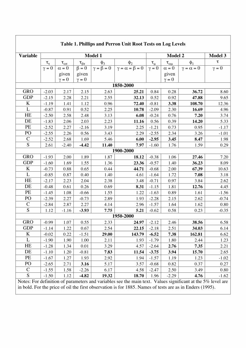
Table 1. Phillips and Perron Unit Root Tests on Log Levels

Model 1 Model 2 Model 3 ττ τατ τβτ φ3 φ2 τµ ταµ φ1 τ

Variable

γ = 0 α = 0 given γ = 0

β = 0 given γ = 0

γ = β = 0

γ = α = β = 0

γ = 0 α = 0 given γ = 0

γ = α = 0

γ = 0

1850-2000 GRO -2.03 2.17 2.15 2.63 25.21 0.84 0.28 36.72 8.60 GDP -2.15 2.28 2.21 2.55 32.13 0.52 0.92 47.88 9.65

K -1.19 1.41 1.12 0.96 72.40 -0.81 3.38 108.70 12.36 L -0.87 0.91 0.52 2.25 10.78 -2.09 2.30 16.69 4.96

HE -2.50 2.58 2.48 3.13 6.08 -0.24 0.76 7.20 3.74 DE -1.83 2.06 2.03 2.23 11.16 0.56 0.39 14.20 5.33 PE -2.52 2.27 -2.16 3.19 2.25 -1.21 0.73 0.95 -1.17 PO -2.55 2.26 0.56 3.43 2.29 -2.55 2.34 3.26 -1.01 C -2.52 2.68 1.69 5.46 6.00 -2.95 3.45 8.47 1.98 S 2.61 -2.40 -4.42 11.40 7.97 -1.60 1.76 1.59 0.29

1900-2000 GRO -1.93 2.00 1.89 1.87 18.12 -0.38 1.06 27.46 7.20 GDP -1.60 1.69 1.55 1.36 23.36 -0.57 1.40 36.23 8.09

K -0.73 0.88 0.65 0.44 44.71 -0.68 2.00 67.39 10.63 L -0.85 0.87 0.40 1.40 4.61 -1.64 1.72 7.08 3.18

HE -2.17 2.23 2.04 2.38 3.48 -0.71 0.97 3.84 2.62 DE -0.48 0.61 0.26 0.69 8.31 -1.15 1.81 12.76 4.45 PE -1.45 1.08 -0.66 1.55 1.22 -1.63 0.89 1.61 -1.56 PO -2.39 2.27 -0.73 2.89 1.93 -2.28 2.15 2.62 -0.74 C -2.84 2.87 2.27 4.14 2.96 -1.57 1.64 1.62 0.80 S 1.12 -1.16 -3.93 7.75 5.21 -0.62 0.58 0.23 -0.35

1950-2000 GRO -0.99 1.07 0.55 2.33 24.97 -2.12 2.46 38.56 6.58 GDP -1.14 1.22 0.67 2.54 22.15 -2.18 2.51 34.03 6.14

K -0.02 0.22 -1.51 29.00 143.79 -6.52 7.38 162.81 6.62 L -1.90 1.90 1.00 2.11 1.93 -1.79 1.80 2.44 1.23

HE -1.28 1.34 0.01 3.29 4.57 -2.64 2.76 7.35 2.21 DE -1.10 1.20 -0.81 7.83 11.54 -3.75 3.94 15.70 2.65 PE -1.67 1.27 1.93 2.92 1.94 -1.57 1.19 1.23 -1.02 PO -2.65 2.71 3.16 5.17 3.57 -0.68 0.82 0.37 0.27 C -1.55 1.58 -2.26 6.17 4.58 -2.47 2.50 3.49 0.80 S -1.50 1.12 -4.82 19.32 18.70 1.96 -2.29 4.76 -1.62

Notes: For definition of parameters and variables see the main text. Values significant at the 5% level are in bold. For the price of oil the first observation is for 1885. Names of tests are as in Enders (1995).

Table 2. Phillips and Perron Unit Root Tests on First Differences of Logs

Model 1 Model 2 Model 3 ττ τατ τβτ φ3 φ2 τµ ταµ φ1 τ

Variable

γ = 0 α = 0 given γ = 0

β = 0 given γ = 0

γ = β = 0

γ = α = β = 0

γ = 0 α = 0 given γ = 0

γ = α = 0

γ = 0

1850-2000 GRO -13.24 7.07 1.22 87.62 58.41 -13.15 7.02 86.40 -10.09 GDP -12.25 7.72 0.64 75.00 50.00 -12.26 7.73 75.11 -8.49

K -3.57 3.28 -0.79 6.47 4.31 -3.52 3.22 6.18 -1.27 L -10.06 4.09 -1.60 50.62 33.75 -9.89 3.96 48.93 -8.76

HE -15.66 3.85 0.18 122.67 81.78 -15.71 3.86 123.44 -14.35 DE -12.64 5.47 1.17 79.95 53.30 -12.59 5.43 79.26 -10.86 PE -13.19 -0.80 0.41 87.11 58.08 -13.23 -0.80 87.54 -13.21 PO -7.39 -0.33 0.58 27.30 18.21 -7.40 -0.04 27.38 -7.44 C -15.71 2.80 -2.25 123.33 82.22 -15.12 2.64 114.27 -14.44 S -11.97 1.07 -3.78 71.66 47.77 -11.11 0.91 61.77 -11.09

1900-2000 GRO -9.12 5.77 -0.18 41.55 27.70 -9.16 5.79 41.95 -6.43 GDP -8.77 6.06 -0.40 38.44 25.63 -8.80 6.08 38.74 -5.59

K -2.29 1.99 -0.44 2.64 1.79 -2.27 1.97 2.62 -1.10 L -6.95 2.30 -0.97 24.16 16.11 -6.91 2.26 23.90 -6.46

HE -12.86 2.78 -0.27 82.69 55.13 -12.92 2.79 83.40 -12.02 DE -10.71 4.85 -1.17 57.36 38.24 -10.63 4.80 56.55 -9.00 PE -10.25 -0.87 1.12 52.51 35.01 -10.18 -0.86 51.85 -10.16 PO -6.89 0.14 0.28 23.76 15.84 -6.93 0.14 24.01 -6.97 C -12.57 0.91 -0.55 78.99 52.66 -12.59 0.91 79.24 -12.51 S -10.21 -0.36 -3.67 52.11 34.74 -9.23 -0.31 42.63 -9.26

1950-2000 GRO -4.48 3.68 -1.09 10.52 7.03 -4.48 3.55 10.07 -2.28 GDP -3.81 3.19 -1.02 7.54 5.03 -3.75 3.03 7.03 -1.77

K -2.20 1.97 -1.94 2.44 1.99 -1.02 0.52 1.09 -1.40 L -3.55 0.84 -0.40 6.32 4.22 -3.60 0.85 6.49 -3.54

HE -8.01 2.37 -1.99 32.22 21.55 -7.32 2.08 26.86 -6.77 DE -8.19 3.81 -3.43 33.65 22.52 -6.75 2.84 22.87 -5.87 PE -4.77 0.13 1.44 11.39 7.64 -4.53 0.15 10.33 -4.59 PO -5.52 0.59 1.60 15.29 10.23 -5.22 0.56 13.65 -5.26 C -8.30 1.29 -3.15 34.42 22.96 -7.17 1.03 25.75 -7.11 S -6.72 -3.31 -4.04 22.69 15.15 -4.82 -1.95 11.65 -4.30

Notes: For definition of parameters and variables see the main text. Values significant at the 5% level are in bold. For the price of oil the first observation is for 1885. Names of tests are as in Enders (1995).

Table 3. KPSS Unit Root Tests

Log Levels Log First Differences Variable H0: Levels Stationary

H0: Trend Stationary

H0: Levels Stationary

H0: Trend Stationary

1850-2000 GRO 3.10 0.58 0.23 0.08 GDP 3.11 0.50 0.15 0.09

K 3.09 0.37 0.19 0.18 L 3.08 0.46 0.39 0.06

HE 3.04 0.37 0.08 0.08 DE 3.02 0.59 0.41 0.26 PE 2.65 0.26 0.09 0.09 PO 0.73 0.17 0.07 0.04 C 2.84 0.45 0.45 0.04 S 2.36 0.49 1.03 0.20

1900-2000 GRO 2.12 0.22 0.09 0.09 GDP 2.12 0.21 0.12 0.11

K 2.12 0.28 0.31 0.31 L 2.01 0.45 0.31 0.06

HE 2.06 0.21 0.10 0.10 DE 2.09 0.25 0.30 0.21 PE 1.64 0.26 0.17 0.07 PO 0.63 0.19 0.06 0.06 C 1.83 0.18 0.08 0.06 S 0.65 0.42 0.90 0.19

1950-2000 GRO 1.09 0.27 0.53 0.10 GDP 1.08 0.27 0.48 0.10

K 1.09 0.29 0.97 0.10 L 0.83 0.20 0.12 0.05

HE 0.91 0.26 0.59 0.07 DE 0.93 0.28 0.82 0.08 PE 0.26 0.22 0.35 0.07 PO 0.75 0.19 0.33 0.08 C 0.38 0.27 0.67 0.10 S 0.85 0.29 0.91 0.10

Notes: For definition of parameters and variables see the main text. Values significant at the 5% level are in bold. For the price of oil the first observation is for 1885.

Table 4. Causality Tests: Production Function Models

Model Period Energy -> GDP GDP -> Energy 1850-2000 0.7574

(0.555) 2.7974 (0.029)

1900-2000 1.6289 (0.174)

2.9700 (0.024)

Bivariate GDP & HE

1950-2000 0.6052 (0.661)

2.392 (0.068)

1850-2000 2.8180 (0.028)

0.6485 (0.629)

1900-2000 2.440 (0.053)

0.7242 (0.578)

Bivariate GDP & DE

1950-2000 0.7751 (0.548)

2.0651 (0.105)

1850-2000 2.3686 (0.056)

1.6173 (0.174)

1900-2000 1.8515 (0.128)

0.588 (0.672)

Multivariate GDP, DE, K, L

1950-2000 1.2092 (0.331)

3.4115 (0.023)

1850-2000 4.5479 (0.002)

0.3397 (0.851)

1900-2000 1.5271 (0.203)

1.4746 (0.218)

Multivariate GRO, DE, K, L

1950-2000 2.9842 (0.037)

2.7127 (0.052)

Notes: All variables are in log levels and all equations include a constant. Number of lags is the selected by the LR test and is the number of lags restricted in the tests. d is the number of additional lags used. The test statistics are F statistics with p-values given in parentheses

Table 5. Causality Tests: Demand Function Models

Model Period Energy -> GDP

Price -> GDP

GDP -> Energy

Price -> Energy

GDP -> Price

Energy -> Price

1850-2000 0.8447 (0.499)

6.7230 (0.000)

2.4157 (0.052)

6.5868 (0.000)

0.9689 (0.427)

2.6133 (0.038)

1900-2000 1.006 (0.412)

5.3176 (0.001)

2.2373 (0.072)

6.4176 (0.000)

0.6615 (0.621)

1.3046 (0.275)

GDP, DE, PE

1950-2000 1.0136 (0.415)

0.3177 (0.864)

5.3721 (0.002)

6.1901 (0.001)

1.5492 (0.212)

0.1994 (0.937)

1850-2000 1.7848 (0.139)

2.7599 (0.032)

2.9792 (0.023)

3.6816 (0.008)

0.3790 (0.823)

0.5074 (0.730)

1900-2000 1.9820 (0.105)

2.5865 (0.042)

2.5345 (0.046)

3.2002 (0.017)

0.2986 (0.878)

0.5596 (0.693)

GDP, HE, PO

1950-2000 0.9804 (0.432)

0.5424 (0.706)

1.8172 (0.150)

1.5731 (0.205)

0.9029 (0.474)

0.2255 (0.922)

Notes: All variables are in log levels and all equations include a constant. Number of lags is the selected by the LR test and is the number of lags restricted in the tests. d is the number of additional lags used. The test statistics are F statistics with p-values given in parentheses

Table 6. VECM Causality Tests

Dependent Variables

Explanatory Variables

Gross Output Capital Labor Divisia Energy 1850-1900

Gross Output 1.7316 (0.132)

0.9974 (0.422)

4.5374 (0.001)

Capital 1.5219 (0.187)

6.067 (0.000)

0.3916 (0.853)

Labor 0.4389 (0.821)

0.7261 (0.605)

0.7261 (0.605)

Divisia Energy 0.4250 (0.830)

0.3995 (0.848)

0.7559 (0.583)

1900-2000 Gross Output 1.6824

(0.148) 2.1965 (0.062)

3.7739 (0.004)

Capital 3.565 (0.006)

3.5442 (0.006)

6.4049 (0.000)

Labor 0.1082 (0.990)

2.0925 (0.075)

0.9616 (0.446)

Divisia Energy 1.0509 (0.394)

0.9331 (0.464)

0.7487 (0.589)

1950-2000 Gross Output 1.8622

(0.128) 0.8006 (0.557)

1.4737 (0.225)

Capital 1.1061 (0.376)

1.2940 (0.290)

1.6958 (0.163)

Labor 1.0676 (0.396)

0.8649 (0.514)

0.8649 (0.515)

Divisia Energy 1.7069 (0.161)

2.7068 (0.037)

0.8056 (0.554)

Notes: Tests are F-statistics for excluding the lags of the respective explanatory variable and the ECM term from the equation. Significance level in parentheses.

Figure 1. Quantity Variables: Sweden 1850-2000

Figure 2. Energy and GDP: Sweden 1850-2000

Figure 3. Growth Rates of GDP and Divisia Index of Energy Use

Figure 4. Energy Prices

Figure 5. Energy, Carbon, and Sulfur Emissions

Figure 6. Carbon Emissions vs. Energy Use