FROM GALLONS TO MILES:

A DISAGGREGATE ANALYSIS OF

AUTOMOBILE TRAVEL AND EXTERNALITY TAXES

Ashley Langer Vikram Maheshri Clifford Winston

University of Arizona University of Houston Brookings Institution

alanger@email.arizona.edu vmaheshri@uh.edu CWinston@brookings.edu

Abstract. Policymakers have prioritized increasing highway revenues as rising fuel economy and

a fixed gasoline tax have led to highway funding deficits. We use a novel disaggregate sample

of motorists to estimate the effect of the price of a vehicle mile traveled on VMT, and provide

the first national assessment of VMT and gasoline taxes that are designed to raise a given amount

of revenue. We find that a VMT tax dominates a gasoline tax on efficiency, distributional and

political grounds when policymakers enact independent fuel economy policies and when the

VMT tax is differentiated with externalities imposed per mile.

January 2017

1

1. Introduction

Personal vehicle transportation is central to the nation’s economic prosperity and to

households’ way of life (Winston and Shirley (1998)). Unfortunately, driving also generates

substantial congestion, pollution, and traffic accident externalities that cost American society

hundreds of billions of dollars per year (Parry, Walls, and Harrington (2007)). Based on the

voluminous literature on consumers’ demand for gasoline,1 economists have paid the most

attention to analyzing policies to reduce pollution and have long argued that gasoline taxes are

more cost effective than Corporate Average Fuel Economy (CAFE) standards because they

encourage motorists to both reduce their driving, measured by vehicle-miles-traveled (VMT),

and to improve their vehicles’ fuel economy.2 In contrast, CAFE does not affect motorists’

VMT in their existing (pre-CAFE vehicles) and it likely increases motorists’ VMT in their new,

post-CAFE vehicles because it improves fuel economy and reduces operating costs.

Unfortunately, policymakers have preferred to increase CAFE standards over time and to

maintain the federal gasoline tax at its 1993 level of 18.4 cents per gallon. This inefficient

approach has been compounded by policymakers’ reliance on gasoline tax revenues to maintain

and expand the highway system. Increasing CAFE standards, while improving the fuel economy

of the nation’s automobile fleet, has led to declines in gas tax revenues per mile and, along with

the fixed gasoline tax, has led to shortfalls in the Highway Trust Fund, which pays for roadway

maintenance and improvements. In fact, the U.S. Treasury has had to transfer more than $140

billion in general funds since 2008 to keep the Highway Trust Fund solvent (U.S. Congressional

Budget Office (2016)). In the midst of this impasse, Congress reiterated its staunch opposition to

1 Havranek, Irsova, and Janda’s (2012) meta-analysis drew on more than 200 estimates of the

price elasticity of gasoline demand. 2 Dahl (1979) conducted an early study of the gasoline tax; more recent work includes Bento et

al. (2009) and Li, Linn, and Muehlegger (2014).

2

raising the gasoline tax when they passed a new five year, $305 billion national transportation

bill in 2015. The U.S. Congressional Budget Office projects that by 2026 the cumulative

shortfall in the highway account will be $75 billion unless additional revenues are raised.3

Facing a limited set of options, some policymakers have become attracted to the idea of

financing highway expenditures by charging motorists and truckers for their use of the road

system in accordance with the amount that they drive, as measured by vehicle-miles-traveled. A

VMT tax has the potential to generate a more stable stream of revenues than a gasoline tax

because motorists cannot reduce their tax burden by driving more fuel efficient vehicles. The

National Surface Transportation Infrastructure Financing Commission recommended that

policymakers replace the gasoline tax with a VMT tax to stabilize transportation funding.

Interest in implementing a VMT tax is growing at the state level on both coasts. Oregon

recruited 5000 volunteers and launched an exploratory study of the effects of replacing its

gasoline tax with a VMT tax. California is conducting a pilot VMT study and the state of

Washington is expected to conduct one. On the east coast, Connecticut, Delaware, New

Hampshire, and Pennsylvania have, as part of the I-95 Corridor Coalition, applied for federal

support to test how a VMT tax could work across multiple states.4

The scholarly economics literature has paid little attention to the economic effects of a

VMT tax because the oil burning externality is a direct function of fuel consumed and because,

3 https://www.cbo.gov/sites/default/files/51300-2016-03-HighwayTrustFund.pdf

4 Moran and Ball (2016) provide a detailed discussion of the Oregon study and suggest that other

states should follow it. The Illinois Senate has proposed legislation to roll back the state’s motor

fuel tax and replace it with a VMT tax within the state’s boundaries. However, Illinois has not

conducted an experiment, and it is not expected that its VMT legislation will be approved.

3

until recently, policymakers have not even mentioned it among possible policy options.5 But

given that (1) policymakers have become increasingly concerned with raising highway revenues

as well as reducing fuel consumption, (2) travelers’ attach utility to VMT, and (3) some

automobile externalities (e.g., congestion and vehicle collisions) accrue more naturally per mile

driven rather than per gallon of fuel consumed, it is important to know whether social welfare is

increased more by a VMT tax than by gasoline taxes that are equivalent in terms of generating

revenue or reducing fuel consumption. And to evaluate the long-run viability of both taxes, it is

important to understand how they interact with separate but related government policies,

including CAFE standards and highway funding that is tied to tax receipts. As we discuss in

detail below, because each tax affects different drivers differently and because both taxes affect

multiple automobile externalities, it is difficult to unambiguously resolve those issues on purely

theoretical grounds.

In this paper, we develop a model of motorists’ short-run demand for automobile travel

measured in vehicle miles that explicitly accounts for heterogeneity across drivers and their

vehicles, and we estimate drivers’ responses to changes in the marginal cost of driving a mile in

their current vehicles. The model allows us to compare the effects of gasoline and VMT taxes on

fuel consumption, vehicle miles traveled, consumer surplus, government revenues, the social

costs of automobile externalities, and social welfare. In theory, a gasoline tax should have the

greatest impact on motorists who are committed to driving the most fuel inefficient vehicles, and

5 An exception is Parry (2005), who calibrated a theoretical model that suggested that VMT taxes

could out-perform gasoline taxes at reducing automobile externalities. The disaggregated

empirical approach that we take here enables us to assess the taxes’ distributional effects by

carefully identifying who is affected by each tax, and to formulate a differentiated VMT tax,

which increases efficiency.

4

a VMT tax should have the greatest impact on motorists who are committed to driving the most

miles.

Our disaggregated empirical approach is able to overcome limitations that characterize

the previous literature on gasoline demand, which has generally used aggregated automobile

transportation and gasoline sales data.6 Aggregate gasoline demand studies specify fuel

consumption or expenditures as the dependent variable and measure the price of travel as dollars

per gallon of gasoline at a broad geographical level. But data that aggregates motorists’ behavior

makes it impossible to determine their individual VMT, vehicle fuel efficiency, or the price that

they normally pay for gasoline. Ignoring those differences and making assumptions about

average fuel economy, gasoline prices, and VMT to construct an aggregate price per mile of

travel will generally lead to biased estimates of the price elasticity of the demand for automobile

travel and hence the economic effects of a VMT tax.7

We initially assess the economic effects of gasoline and VMT taxes that each: (1) reduce

total fuel consumption by 1%, or (2) raise an additional $55 billion per year for highway

spending, which roughly aligns with the annual sums called for by the 2015 federal

transportation bill. Surprisingly, we find that the taxes have very similar effects on social

welfare. But when we account for the recent increase in CAFE standards that calls for

significant improvements in vehicle fuel economy, and when we exploit the flexibility of a VMT

tax by setting different rates for urban and rural driving, we find that a VMT tax designed to

6 McMullen, Zhang, and Nakahara (2010) estimated the behavior of a cross-section of drivers in

Oregon to compare the distributional effects of a VMT tax and a gasoline tax, but a cross-

sectional model cannot control for the potential bias that is caused by unobserved household and

city characteristics that are likely to be correlated with the price of gasoline, vehicle fuel

economy, and vehicle miles driven. 7 Levin, Lewis, and Wolak (2014) find that aggregating gasoline prices tends to reduce the

estimated elasticity of gasoline demand.

5

increase highway spending $55 billion per year increases annual welfare by $10.5 billion or

nearly 20% more than a gasoline tax does because: (1) the differentiated VMT tax is better than

the gasoline tax at targeting its tax to and affecting the behavior of those drivers who create the

greatest externalities, and (2) the greater fuel economy that results from a higher CAFE standard

effectively reduces a gasoline tax and its benefits, but does not affect a VMT tax and its benefits.

Our empirical findings therefore indicate that implementing a VMT tax is a more

efficient policy than raising the gasoline tax to improve the financial and economic condition of

the highway system. Importantly, we also identify considerations that suggest that a VMT tax is

likely to be more politically attractive to policymakers than is raising the gasoline tax.

2. The Short-Run Demand for Automobile Travel

Households’ demand for a given vehicle type and their utilization of that vehicle have

been modeled as joint decisions to facilitate analyses of policies that in the long run may cause

households to change the vehicles they own (e.g., Mannering and Winston (1985)). We conduct

a short-run analysis that treats an individual motorist’s vehicle as fixed; the average length of

time that motorists tend to keep their vehicles suggests that the short run in this case is at least

five years. We discuss later how our findings would be affected if we conducted a long-run

analysis.

Demand Specification

Conditional on owning a particular vehicle, individual i’s use of a vehicle c for a given

time period t is measured by the vehicle-miles-traveled (VMT) accumulated over that time

period, which depends on the individual’s and vehicle’s characteristics, and on contemporaneous

6

economic conditions. We assume that individual i’s utilization equation in period t has a

generalized Cobb-Douglas functional form given by:

𝑉𝑀𝑇𝑐(𝑖)𝑡 = 𝑓𝑐(𝑖)𝜆𝑡𝑝𝑐(𝑖)𝑡𝛽𝑖 (1)

The function 𝑓𝑐(𝑖), which we specify as 𝑓𝑐(𝑖) = exp(𝜆𝑖 + 𝜃𝑍𝑐(𝑖)), contains an individual fixed

effect, 𝜆𝑖, that captures individuals’ unobserved characteristics that affect their utilization of a

vehicle and a vector of vehicle characteristics, 𝑍𝑐(𝑖), excluding fuel economy because it forms

part of the price of driving a mile discussed shortly. To capture heterogeneity among drivers, the

price elasticity, 𝛽𝑖, is specified as 𝛽𝑖 = 𝜓𝑋𝑖, where 𝑋𝑖 includes driver and vehicle characteristics.

The vectors 𝜃 and 𝜓 are estimable parameters.

Note that the price of driving a mile, 𝑝𝑐(𝑖)𝑡, is equal to the price of gasoline in month t for

driver i divided by vehicle c(i)’s fuel economy; thus, this price is likely to vary significantly

across drivers because different vehicles have different fuel economies and because the price of

gasoline varies both geographically and over time. The utilization equation is more general than

a standard Cobb-Douglas demand function for VMT because the price elasticity is allowed to

vary by driver and vehicle characteristics and over time.

To estimate the parameters in equation (1), we take natural logs and combine terms to

obtain the log-linear estimating equation

𝑙𝑜𝑔 𝑉𝑀𝑇𝑖𝑡 = 𝜆𝑖 + 𝜃𝑍𝑐(𝑖) + �̃�𝑡 + 𝛽𝑖 𝑙𝑜𝑔(𝑝𝑐(𝑖)𝑡) + 𝜀𝑖𝑡 (2)

where the tilde denotes the logarithm of the time fixed effects and 𝜀𝑖𝑡 is an error term. All of the

parameters can then be estimated by least squares. We specify the gasoline price as a price per

mile because we are not analyzing vehicle choice; thus, we would expect that the gasoline price

7

would influence the VMT decision only through the price per mile.8 Although we do not have

access to the income of drivers in our sample, we used the average income in a driver’s zip code

and age group to explore including the log of income, but we found that its effect on VMT was

statistically insignificant, in all likelihood because of our imprecise income measure. Thus, we

allow income to have an independent effect on VMT that is captured by the individual driver

fixed effects.

Data

Estimating the model requires us to observe individual drivers’ VMT over time along

with sufficient information about their residential locations and their vehicles to accurately

measure the prices of driving their vehicles. We obtained data from State Farm Mutual

Automobile Insurance Company on individual drivers, who in return for a discount on their

insurance, allowed a private firm to remotely record their vehicles’ exact VMT from odometer

readings (a non-zero figure was always recorded) and to transmit it wirelessly so that it could be

stored.9 All of the vehicles were owned by households and were not part of a vehicle fleet. State

Farm collected a large, monthly sample of drivers in the state of Ohio from August 2009, in the

midst of the Great Recession, to September 2013, which was well into the economic recovery.

The number of distinct household observations in the sample steadily increased from 1,907 in

August 2009 to 9,955 in May 2011 and then stabilized with very little attrition thereafter.10 The

sample consists of 228,910 driver-months.

8 In fact, we found that the gasoline price alone had a statistically insignificant effect on VMT. 9 We are grateful to Jeff Myers of State Farm for his valuable assistance with and explanation of

the data. We stress that no personal identifiable information was utilized in our analysis and that

the interpretations and recommendations in this paper do not necessarily reflect those of State

Farm.

10 Less than 2% of households left the sample on average in each month. This attrition was not

statistically significantly correlated with observed socioeconomic or vehicles characteristics.

8

The drivers included in our sample are State Farm policyholders who are also generally

the heads of their households. The data set included driving information on one vehicle per

household at a given point in time. A driver’s vehicle selection did not appear to be affected by

seasonal or employment-related patterns that would lead to vehicle substitution among

household members because fewer than 2% of the vehicles in the sample were idled in a given

month. In addition, we estimated specifications that included a multi-driver household dummy

to control for the possibility of intra-household vehicle substitution and interacted it with the

price per mile; we found that the parameter for this interaction was statistically insignificant and

that the other parameter estimates changed very little. It is possible that vehicle substitution was

less in our sample than in other household automobile samples because the household head

tended to drive the vehicle that was subject to monitoring by State Farm; thus, we consider later

how our conclusions might be affected if intra-household vehicle substitution occurred more

frequently than in our sample.

The sample also contains information about each driver’s socioeconomic characteristics,

vehicle characteristics, and county of residence, which is where their travel originates.11 To

measure the price of driving one mile over time, we used the average pump price in a driver’s

county of residence for each month from 2009-2013 from data provided by the Oil Price

Information Service. Figure A1 in the appendix plots the county-level average gasoline prices in

each month of our sample and shows that those prices fluctuated greatly over time, which

11 According to the most recent National Household Travel Survey (NHTS) taken in 2009,

roughly half of all vehicle trips were less than 5 miles, suggesting that driving is concentrated in

individuals’ counties of residence. The NHTS is available at:

http://nhts.ornl.gov

9

accounted for most of its variation in the sample; however, average gasoline prices also varied

across counties within a month.12

Given the low rate of intra-household vehicle substitution and our inclusion of individual

fixed effects, we are able to identify the effect of changes in gasoline prices on individual

motorists’ VMT. We measured the fuel economy of the driver’s vehicle by using the vehicle’s

VIN to find the vehicle year, make, model, body style, and engine type and matched that

information to the Environmental Protection Agency’s (EPA) database of fuel economies.13

Following the EPA, we used the combined fuel economy for each vehicle, which is the weighted

average of the vehicle’s fuel economy on urban and highway drive cycles. Finally, as noted,

because State Farm does not collect individual drivers’ income, we allowed income to be entirely

absorbed by the individual fixed effects.

Table 1 reports the means in our sample (and, when publicly available, the means in

Ohio, and the United States) of drivers’ average monthly VMT, the components of the price of

driving one mile, vehicle miles per gallon and the local price of a gallon of gasoline, the

percentage of older vehicles, average annual income, and the percentage of the county

12 The ordering of counties’ average gasoline prices also changed considerably over time. Nearly

50% of the time that a county’s gasoline prices were in the bottom quartile in a given month, that

county’s prices were not in the bottom quartile in the following month, and nearly 30% of the

time that a county’s gasoline prices were in the top quartile in a given month, that county’s prices

were not in the top quartile in the following month. We obtained additional evidence of the

variation in gasoline prices by analyzing the residuals of a regression of county-month gasoline

prices on county and month fixed effects. We found that the residuals ranged from -19 cents to

+22 cents with a standard deviation of 3 cents. The correlation between those residuals and their

one-month within-county lag was only 0.31, suggesting that substantial variation in gas prices

exists beyond county and month fixed effects.

13 We are grateful to Florian Zettelmeyer and Christopher Knittel for assistance in matching

VINs to vehicle attributes.

10

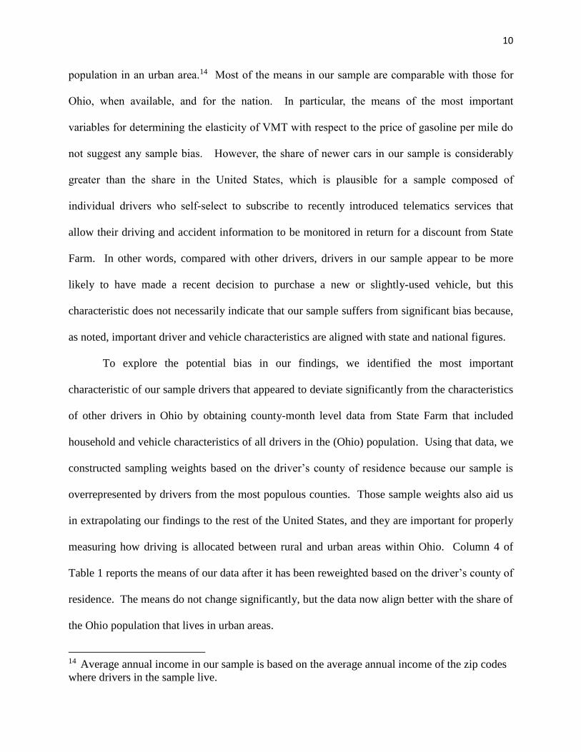
population in an urban area.14 Most of the means in our sample are comparable with those for

Ohio, when available, and for the nation. In particular, the means of the most important

variables for determining the elasticity of VMT with respect to the price of gasoline per mile do

not suggest any sample bias. However, the share of newer cars in our sample is considerably

greater than the share in the United States, which is plausible for a sample composed of

individual drivers who self-select to subscribe to recently introduced telematics services that

allow their driving and accident information to be monitored in return for a discount from State

Farm. In other words, compared with other drivers, drivers in our sample appear to be more

likely to have made a recent decision to purchase a new or slightly-used vehicle, but this

characteristic does not necessarily indicate that our sample suffers from significant bias because,

as noted, important driver and vehicle characteristics are aligned with state and national figures.

To explore the potential bias in our findings, we identified the most important

characteristic of our sample drivers that appeared to deviate significantly from the characteristics

of other drivers in Ohio by obtaining county-month level data from State Farm that included

household and vehicle characteristics of all drivers in the (Ohio) population. Using that data, we

constructed sampling weights based on the driver’s county of residence because our sample is

overrepresented by drivers from the most populous counties. Those sample weights also aid us

in extrapolating our findings to the rest of the United States, and they are important for properly

measuring how driving is allocated between rural and urban areas within Ohio. Column 4 of

Table 1 reports the means of our data after it has been reweighted based on the driver’s county of

residence. The means do not change significantly, but the data now align better with the share of

the Ohio population that lives in urban areas.

14 Average annual income in our sample is based on the average annual income of the zip codes

where drivers in the sample live.

11

3. Estimation results

An estimate of the price elasticity of VMT that varies with driver and vehicle

characteristics, 𝛽𝑖 = 𝜓𝑋𝑖, is of primary interest for our analysis. Identification of the parameters

𝜓 is achieved through individual drivers’ differential responses to changes in the price of

gasoline per mile based on the fuel economy of their vehicles. Biased estimates of 𝜓 would

therefore arise from omitted variables that are correlated with gasoline prices and that affect

drivers’ VMT differently based on their vehicles’ fuel economy. As noted, the drivers’ fixed

effects capture their unobserved characteristics that may be correlated with observed influences

on VMT, especially the price of driving one mile that is constructed in part from the fuel

economy of the drivers’ vehicles. In addition, macroeconomic and weather conditions could

affect the price of gasoline paid by drivers and how much they traveled by automobile. Thus we

controlled for that potential source of bias by including county level macroeconomic variables

(the unemployment rate, the percent of population in urban areas, employment, real GDP, and

average wages and compensation) and weather variables (the number of days in a month with

precipitation and the number of days in a month with a minimum temperature of less than or

equal to 32 degrees).15

Drivers’ responses to a change in the price per mile could vary in accordance with a

number of factors, including how much they drive, whether they live in an urban or rural area,

15 Data on the county level unemployment rate and level of employment, average wages and

compensation, and real GDP are from the U.S. Bureau of Labor Statistics; data on the percent of

population in urban areas are from the U.S. Census; and monthly weather data are from the

National Climatic Data Center of the National Oceanographic and Atmospheric Administration.

12

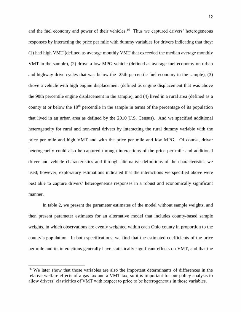
and the fuel economy and power of their vehicles.16 Thus we captured drivers’ heterogeneous

responses by interacting the price per mile with dummy variables for drivers indicating that they:

(1) had high VMT (defined as average monthly VMT that exceeded the median average monthly

VMT in the sample), (2) drove a low MPG vehicle (defined as average fuel economy on urban

and highway drive cycles that was below the 25th percentile fuel economy in the sample), (3)

drove a vehicle with high engine displacement (defined as engine displacement that was above

the 90th percentile engine displacement in the sample), and (4) lived in a rural area (defined as a

county at or below the 10th percentile in the sample in terms of the percentage of its population

that lived in an urban area as defined by the 2010 U.S. Census). And we specified additional

heterogeneity for rural and non-rural drivers by interacting the rural dummy variable with the

price per mile and high VMT and with the price per mile and low MPG. Of course, driver

heterogeneity could also be captured through interactions of the price per mile and additional

driver and vehicle characteristics and through alternative definitions of the characteristics we

used; however, exploratory estimations indicated that the interactions we specified above were

best able to capture drivers’ heterogeneous responses in a robust and economically significant

manner.

In table 2, we present the parameter estimates of the model without sample weights, and

then present parameter estimates for an alternative model that includes county-based sample

weights, in which observations are evenly weighted within each Ohio county in proportion to the

county’s population. In both specifications, we find that the estimated coefficients of the price

per mile and its interactions generally have statistically significant effects on VMT, and that the

16 We later show that those variables are also the important determinants of differences in the

relative welfare effects of a gas tax and a VMT tax, so it is important for our policy analysis to

allow drivers’ elasticities of VMT with respect to price to be heterogeneous in those variables.

13

estimated coefficients of the interactions affect the magnitude of the estimated baseline

coefficient of the price per mile in plausible ways. Specifically, drivers with high VMT have a

lower price elasticity (in absolute value) compared with other drivers’ elasticity, in all likelihood

because their longer distance commutes and non-work trips that contribute to their high VMT,

regardless of whether they live in urban or rural areas, make it less likely that they can adjust

their VMT in response to changes in the price per mile. Drivers of vehicles that have low MPG

have higher vehicle operating costs per mile than other drivers, which gives them a greater

economic incentive to adjust their VMT in response to changes in the price per mile. All else

constant, drivers who live in rural areas may be more price sensitive than other drivers because

they are generally less affluent than drivers who live in more urbanized areas. But both high

VMT and low MPG rural drivers are apparently less able or willing than other rural drivers are to

adjust their automobile work and non-work trips and thus less likely than other rural drivers are

to adjust their VMT in response to changes in the price per mile. Finally, drivers of powerful

vehicles with high engine displacement, and undoubtedly a higher sticker price, tend to be more

affluent than other drivers are and less inclined to adjust their VMT in response to changes in the

price per mile.

The variation in our data, which underlies the statistical significance of the price variable

and its interactions with driver and vehicle characteristics, is that vehicle fuel economy ranges

from 12 to 34 miles per gallon, which when combined with the variation in the price of gasoline

implies a price of driving one mile that ranges from 8.6 cents to 33.7 cents. We stress that it

would not be possible to estimate the heterogeneous, or even homogeneous, effects of the price

per mile on VMT with aggregate data because VMT could not be expressed as a function of the

price of automobile travel per mile.

14

The price elasticities obtained from the two models for drivers who do not have high

VMT, do not have a vehicle with low MPG or high engine displacement, and do not live in rural

areas are virtually identical and their magnitude of -0.17 is plausible. Accounting for all the

interactions, the range of the elasticities for both models is roughly -0.60 to slightly greater than

zero, which is also plausible given the significant heterogeneity that we capture.17 Furthermore,

given that the second set of parameter estimates incorporates sample weights, the ability of the

State Farm sample to generate price elasticities that are representative of the population does not

appear to be affected much by households’ self-selection to subscribe to telematics services.

To get a feel for how the elasticities compare with elasticities obtained from aggregate

gasoline demand models, we note that in the preferred specification that was estimated with

sample weights, the average elasticity of VMT with respect to the price of automobile travel per

mile is -0.117. We estimated that the elasticity of the demand for gasoline with respect to

gasoline prices was -0.124 in our sample, which is somewhat larger than the average short-run

elasticity of -0.09 reported in Havranek, Irsova, and Janda’s (2012) meta-analysis of aggregate

models, and it is noticeably larger than our own estimate of the aggregate price elasticity of

demand for gasoline in Ohio of -0.0407 (0.0099) and the range of aggregate elasticity estimates

for the nation, -0.034 to -0.077, in Hughes, Knittel, and Sperling (2008). We attribute this

difference to our use of disaggregate data, which as Levin, Lewis, and Wolak (2014) find, results

in higher estimates of gasoline demand elasticities.

17 The drivers with slightly positive elasticities appear to be quite unusual because they have high

VMT, drive vehicles with high engine displacement, do not drive vehicles with low fuel

economy, and do not live in rural areas. Accordingly, they account for less than 0.5% of the

drivers in our sample.

15

Finally, we explored the direct effect on VMT of various vehicle types, based on size

classification, and vehicle attributes and we found some statistically significant effects. Table 2

shows that SUVs tend to be driven more per month than other household vehicles, in all

likelihood because those vehicles are versatile and can be used for both work and various non-

work trips, while older vehicles tend to be driven less per month than newer vehicles, in all

likelihood because drivers enjoy using newer vehicles and their up-to-date accessories for a

broad variety of trips.18

We explored alternative specifications of the VMT demand model to enrich the analysis

and to perform robustness checks. We tested whether our results were affected by time-varying

unobservables by estimating separate regressions on several subsamples of shorter length. This

change resulted in coefficients that reflected seasonal patterns, but did not reveal any

fundamental differences in their underlying values. In addition, we estimated models that

included lagged prices per mile to capture any adjustments by motorists to price changes, but the

lags tended to be statistically insignificant and their inclusion only slightly reduced the estimated

effects of the current price per mile, although the combined effect of current and lagged gasoline

prices was similar to the effect reported here. More importantly, even if motorists delayed their

responses to price changes, our main policy simulations would not be affected because we assess

the economic effects of a permanent increase in either the gasoline or VMT tax.

4. Welfare Analysis

18 The relationship between VMT and SUVs and older vehicles is identified based on households

who own more than one vehicle in our sample over time, which means that within a household,

SUVs tend to be driven more than non-SUVs and newer vehicles tend to be driven more than

older vehicles.

16

The gasoline tax is currently used to charge motorists and truckers for their use of the

public roads, to raise highway revenues, and to encourage motorists and truckers to reduce fuel

consumption. However, as noted, the federal component of the tax has not been raised in

decades and the Highway Trust Fund is currently running a deficit that is projected to grow

substantially unless more funds are provided to maintain and repair the highway system.19 It is

therefore of interest to assess the social welfare effects of raising the federal gasoline tax or,

alternatively, of introducing a VMT tax to achieve both highway financing objectives and to

reduce externalities from fuel consumption and highway travel.

Advances in communications technology have made it possible to implement a VMT tax

in any state in the country. Specifically, an inexpensive device can be installed in vehicles that

tracks mileage driven in states and wirelessly uploads this information to private firms to help

states administer the program. Motorists are then charged lump sum for their use of the road

system each pay period, which is normally a month. For example, the cost of Oregon’s

experimental VMT tax program is $8.4 million. For privacy reasons, data older than 30 days are

deleted once drivers pay their VMT tax bills.

We use our estimates of VMT demand with county population weights as our preferred

model to extrapolate our results for Ohio to the United States. The effect on social welfare of a

gasoline or VMT tax that is designed to achieve a certain change in fuel consumption or highway

finance consists of (a) changes in motorists’ welfare and government revenues and (b) changes in

the relevant pollution, congestion, and safety automobile externalities. Motorists’ welfare is

adversely affected because the taxes will cause them to reduce their vehicle miles traveled by

19 Some states have raised their gasoline tax in recent decades.

17

automobile, which they highly value (Winston and Shirley (1998)). Similar to Hausman (1981),

we obtain the short-run indirect utility function for each motorist given by:

𝑉𝑖𝑡(𝑝) = 𝑓𝑐(𝑖)𝜆𝑡

𝑝𝑐(𝑖)𝑡

𝛽𝑖+1

𝛽𝑖+1+ 𝐶 (3)

where C is a constant of integration and other variables and parameters are as defined

previously.20 Under a gasoline or VMT tax that changes the price of driving one mile from 𝑝𝑖𝑡0 to

𝑝𝑖𝑡1 , the change in driver i’s welfare is given by 𝑉𝑖𝑡(𝑝𝑖𝑡

1 ) − 𝑉𝑖𝑡(𝑝𝑖𝑡0 ), and we can aggregate the

effects of a tax policy over all drivers as:

𝛥𝑉𝑡 = ∑ 𝑉𝑖𝑡(𝑝𝑖𝑡1 ) − 𝑉𝑖𝑡(𝑝𝑖𝑡

0 )𝑖 . (4)

Note that the original prices per mile, 𝑝𝑖𝑡0 , the counterfactual prices 𝑝𝑖𝑡

1 , and the changes in

consumer surplus are likely to vary significantly across individual motorists because they drive

different vehicles, use them different amounts, and respond differently to changes in the price per

mile in accordance with their VMT, residential location, and their vehicles’ fuel economy and

engine displacement. A gasoline tax and a VMT tax have different effects on the change in the

cost of driving a mile for almost every driver because the VMT tax increases the cost of driving a

mile by the amount of the tax, while the gasoline tax increases the cost of driving a mile by the

amount of the per-gallon tax divided by the individual driver’s fuel economy. Thus, a VMT tax

increases the price of driving a mile by the largest percentage for drivers of fuel efficient vehicles

because it is a fixed charge and because drivers of fuel-efficient vehicles incur the lowest

operating cost per mile, while a gasoline tax increases the price of driving a mile the most for

drivers of fuel-inefficient vehicles.

20 We obtain the indirect utility function in equation (3) by applying Roy’s Identity to the VMT

demand equation (1) and by assuming a constant marginal utility of income to facilitate welfare

analysis.

18

If we denote the change in government revenues by 𝛥𝐺𝑡 and the change in the cost of

automobile externalities by 𝛥𝐸𝑡, then the change in social welfare from either a gasoline or VMT

tax, 𝛥𝑊𝑡, is given by

𝛥𝑊𝑡= 𝛥𝑉𝑡 + 𝛥𝐺𝑡 + 𝛥𝐸𝑡. (5)

In order to calculate 𝛥𝐸𝑡, we need estimates of the marginal external cost of using a

gallon of gasoline and of driving both urban and rural miles. We measure the external cost per

gallon of gasoline consumed by including its climate externality. We use the Energy

Information Agency’s estimate of 19.564 pounds of CO2 equivalent emissions per gallon of gas

consumed and the Environmental Protection Agency’s midrange estimate of the social cost of

carbon of $40 per ton of CO2 in 2015 to obtain a marginal externality cost of $0.393/gallon.21

The per mile marginal external cost consists of: (1) the congestion externality (including

both the increased travel time and increased unreliability of travel time), (2) the accident

externality, and (3) the local environmental externalities of driving. We use estimates from

Small and Verhoef (2007), which are broadly consistent with estimates in Parry, Walls, and

Harrington (2007), adjusted to 2013 dollars and divided into urban and rural values of

$0.218/urban mile driven and $0.038/rural mile driven.22 The estimates developed by those

21 http://www3.epa.gov/climatechange/EPAactivities/economics/scc.html. Note that this estimate

of the climate externality is substantially higher than the estimates used by Parry (2005), Parry

and Small (2005), and Small and Verhoef (2007) because it incorporates more recent advances in

estimating the social cost of carbon that feed into the EPA’s current estimate of this social cost.

22 For the increased travel time externality, we use $0.049/mi for urban drivers and $0.009/mi for

rural drivers and following Small and Verhoef (2007), we multiply those values by 0.93 to get

the marginal external cost of decreased travel time reliability and add this cost to the cost of

increased travel time to obtain a total congestion externality of $0.129/mi for urban drivers and

$0.023/mi for rural drivers. The accident externality for urban drivers adapted from Small and

Verhoef is $0.073/mi. We use the ratio of the rural and urban congestion externalities to

approximate the rural accident externality of $0.013/mi. Finally, following Small and Verhoef

(2007), Parry (2005), and Parry and Small (2005), we assume that the local pollutant externality

19

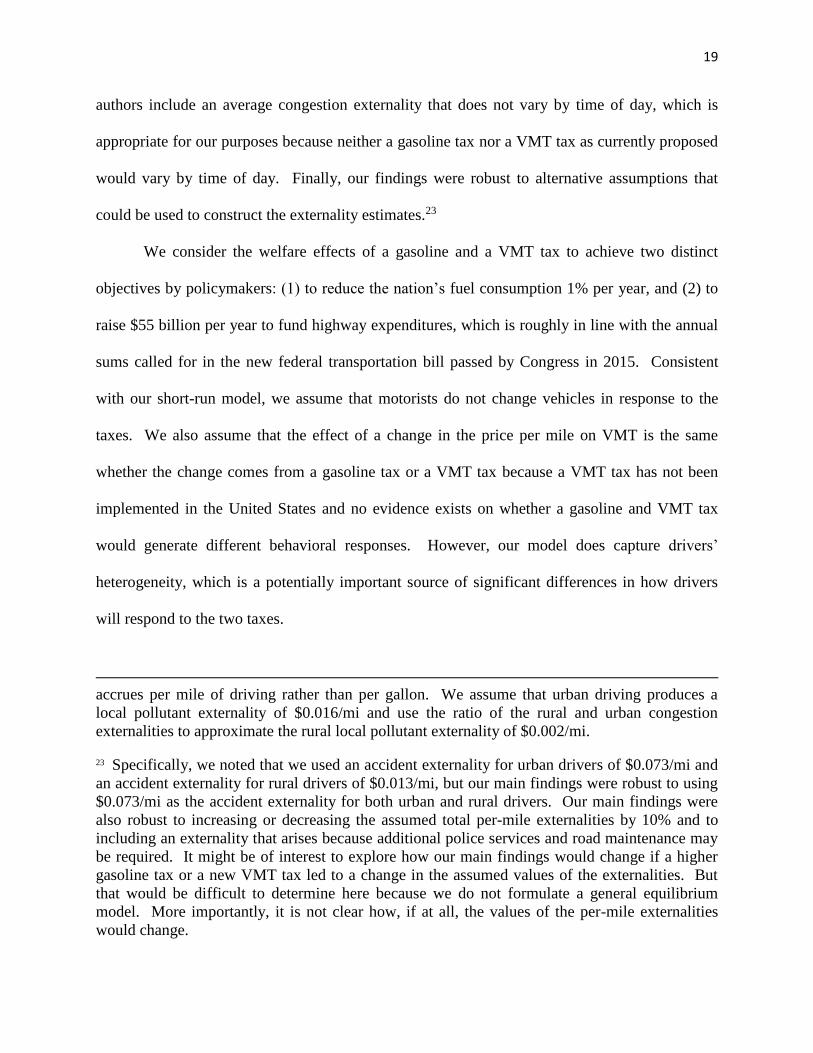
authors include an average congestion externality that does not vary by time of day, which is

appropriate for our purposes because neither a gasoline tax nor a VMT tax as currently proposed

would vary by time of day. Finally, our findings were robust to alternative assumptions that

could be used to construct the externality estimates.23

We consider the welfare effects of a gasoline and a VMT tax to achieve two distinct

objectives by policymakers: (1) to reduce the nation’s fuel consumption 1% per year, and (2) to

raise $55 billion per year to fund highway expenditures, which is roughly in line with the annual

sums called for in the new federal transportation bill passed by Congress in 2015. Consistent

with our short-run model, we assume that motorists do not change vehicles in response to the

taxes. We also assume that the effect of a change in the price per mile on VMT is the same

whether the change comes from a gasoline tax or a VMT tax because a VMT tax has not been

implemented in the United States and no evidence exists on whether a gasoline and VMT tax

would generate different behavioral responses. However, our model does capture drivers’

heterogeneity, which is a potentially important source of significant differences in how drivers

will respond to the two taxes.

accrues per mile of driving rather than per gallon. We assume that urban driving produces a

local pollutant externality of $0.016/mi and use the ratio of the rural and urban congestion

externalities to approximate the rural local pollutant externality of $0.002/mi. 23 Specifically, we noted that we used an accident externality for urban drivers of $0.073/mi and

an accident externality for rural drivers of $0.013/mi, but our main findings were robust to using

$0.073/mi as the accident externality for both urban and rural drivers. Our main findings were

also robust to increasing or decreasing the assumed total per-mile externalities by 10% and to

including an externality that arises because additional police services and road maintenance may

be required. It might be of interest to explore how our main findings would change if a higher

gasoline tax or a new VMT tax led to a change in the assumed values of the externalities. But

that would be difficult to determine here because we do not formulate a general equilibrium

model. More importantly, it is not clear how, if at all, the values of the per-mile externalities

would change.

20

Our initial simulations also assume that the government requires automakers to continue

to meet the current CAFE standard, which forces motorists into more fuel efficient vehicles than

they might otherwise drive. In subsequent simulations, we explore how the economic effects of

a gas or VMT tax would vary in the presence of a higher CAFE standard. By improving fuel

efficiency, CAFE standards could induce a rebound effect, but it is not necessary for us to

assume a particular magnitude of that effect here to analyze the economic effects of a gasoline or

VMT tax.

Because we are analyzing heterogeneous drivers and vehicles, economic theory cannot

unambiguously indicate whether a gasoline tax or a VMT tax will produce a larger improvement

in social welfare. But it is useful to identify the important influences on the welfare effects of

the two taxes and the conditions under which one will generate a larger welfare gain than the

other. Recall, that the additional per mile cost to a driver of a VMT tax is just the VMT tax,

while the additional per mile cost of a gasoline tax is the gas tax divided by the vehicle’s fuel

economy. Figure 1 presents a flow chart that: (1) identifies the important driver and vehicle

characteristics that determine the welfare effects of each tax, and (2) shows how the

heterogeneity of drivers and their vehicles culminate in certain conditions whereby the gasoline

tax generates a larger welfare gain than a VMT tax produces and vice-versa.

The important characteristics are a vehicle’s fuel economy, which for heterogeneous

vehicles we denote as a low MPG or a high MPG vehicle; a driver’s vehicle utilization, which

for heterogeneous drivers we denote as low VMT or high VMT; and a driver’s gasoline price

elasticity of demand, ε, which for heterogeneous drivers we denote as low ε or high ε. We

assume we are not fully internalizing the observed fuel consumption, congestion, and safety

automobile externalities; thus, social welfare is improved by taxes that increase a driver’s cost

21

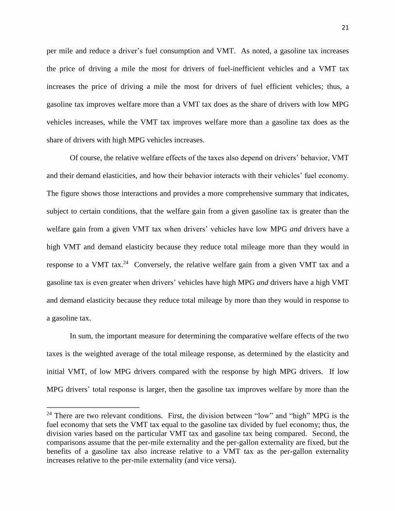
per mile and reduce a driver’s fuel consumption and VMT. As noted, a gasoline tax increases

the price of driving a mile the most for drivers of fuel-inefficient vehicles and a VMT tax

increases the price of driving a mile the most for drivers of fuel efficient vehicles; thus, a

gasoline tax improves welfare more than a VMT tax does as the share of drivers with low MPG

vehicles increases, while the VMT tax improves welfare more than a gasoline tax does as the

share of drivers with high MPG vehicles increases.

Of course, the relative welfare effects of the taxes also depend on drivers’ behavior, VMT

and their demand elasticities, and how their behavior interacts with their vehicles’ fuel economy.

The figure shows those interactions and provides a more comprehensive summary that indicates,

subject to certain conditions, that the welfare gain from a given gasoline tax is greater than the

welfare gain from a given VMT tax when drivers’ vehicles have low MPG and drivers have a

high VMT and demand elasticity because they reduce total mileage more than they would in

response to a VMT tax.24 Conversely, the relative welfare gain from a given VMT tax and a

gasoline tax is even greater when drivers’ vehicles have high MPG and drivers have a high VMT

and demand elasticity because they reduce total mileage by more than they would in response to

a gasoline tax.

In sum, the important measure for determining the comparative welfare effects of the two

taxes is the weighted average of the total mileage response, as determined by the elasticity and

initial VMT, of low MPG drivers compared with the response by high MPG drivers. If low

MPG drivers’ total response is larger, then the gasoline tax improves welfare by more than the

24 There are two relevant conditions. First, the division between “low” and “high” MPG is the

fuel economy that sets the VMT tax equal to the gasoline tax divided by fuel economy; thus, the

division varies based on the particular VMT tax and gasoline tax being compared. Second, the

comparisons assume that the per-mile externality and the per-gallon externality are fixed, but the

benefits of a gasoline tax also increase relative to a VMT tax as the per-gallon externality

increases relative to the per-mile externality (and vice versa).

22

VMT tax does. If high MPG drivers’ total response is larger, then the VMT tax improves

welfare by more than the gasoline tax does.

Initial Findings

In the initial simulations presented in tables 3 and 4, we compare the effects of a 31.2

cent per gallon gasoline tax and a 1.536 cent per mile VMT tax because each tax reduces total

fuel consumption by 1 percent, and we compare the effects of a 40.8 cent per gallon gasoline tax

and a 1.99 cent per mile VMT tax because each tax raises $55 billion per year for highway

spending. In light of the preceding discussion that explained why heterogeneous drivers could

potentially have different responses to the two taxes and that the taxes could potentially have

different welfare effects, it is surprising that we find that the gasoline and VMT taxes have

remarkably similar effects on the nation’s social welfare in the process of reducing fuel

consumption and raising highway revenues.25

The gasoline and VMT taxes reduce fuel consumption 1%, while they increase annual

welfare by $5.1 billion and $5.3 billion respectively via reductions in the various external costs,

especially congestion and accidents, with the loss in consumer surplus and increase in

government revenues essentially offsetting each other. We reach virtually the same conclusion

for a gasoline and VMT tax that each raise $55 billion per year for highway spending, as annual

welfare is increased by $6.5 billion and $6.7 billion respectively. To be sure, our externality

25 All gasoline and VMT taxes presented in our simulation results are in addition to the state and

federal gasoline taxes that currently exist. In order to use our sample of Ohio motorists to

extrapolate results to the national level, we used the results from our sample for March 2013 and

assumed that it was reasonable to scale them so they applied for an entire year. We used our

county-level weights to get an annual estimate of the welfare effects for the state of Ohio and

then scaled that result to the nation by assuming that an Ohio resident was representative of a

U.S. resident in March 2013 (using an inflator of 316.5 million (U.S. Population)/11.5 million

(Ohio Population)).

23

estimates suggest that the externality per mile is substantially larger than the externality per

gallon that is expressed per mile, which suggests that a given decrease in VMT would reduce

automobile externalities more than would a comparable decrease in gasoline consumption.26 But

from the perspective of the framework in figure 1, we did not find notable differences in the

welfare effects of the two taxes because the weighted average of the mileage responses of the

various sub-groups that comprise drivers of high fuel-economy vehicles and that comprise

drivers of low fuel-economy vehicles was similar.

We stress that without a disaggregate model, we could not perform the preceding

simulations because it would be very difficult to know the magnitude of the VMT tax that is

appropriate to compare with a gasoline tax to achieve the same reduction in fuel consumption

and the same increase in highway revenues, and to properly account for the change in

externalities that is critical for the welfare assessment.

Extending the Analysis

As noted, policymakers have generally preferred to use tighter Corporate Average Fuel

Economy standards to increase fuel economy.27 But by raising overall fuel economy and fuel

economy for certain types of vehicles, a change in CAFE standards will also change the effect of

a VMT tax or increased gasoline tax on welfare. Indeed, the most recent CAFE standards call

for new passenger cars and light trucks to achieve average (sales-weighted) fuel efficiencies that

were projected to be as high as 34.1 miles-per-gallon by 2016 and 54.5 miles-per-gallon by 2025.

To meet those standards, it is reasonable to assume that over time average vehicle fuel efficiency

26 Parry (2005) reached a similar conclusion based on the parameter values he assumed. 27 Higher gasoline taxes (or the introduction of a VMT tax) might also induce automobile firms to

innovate more in fuel efficiency. For example, Aghion et al. (2016) find that higher tax-

inclusive fuel prices encourage automobile firms to innovate in clean technologies.

24

will improve considerably from its current sales-weighted average of roughly 25 miles-per-

gallon. Because it is not clear how, if at all, other attributes of a vehicle may change with more

stringent fuel economy standards, we assume other non-price vehicle attributes remain

constant.28

Another relevant consideration for our analysis is that because the (marginal) costs of

local pollution and congestion externalities associated with driving are significantly greater in

urban areas than they are in rural areas, efficiency could be enhanced by differentiating a VMT

tax in urban and rural geographical areas to reflect the different externality costs. As described

earlier, the technology that is used to implement a state-wide VMT tax could be refined to

differentiate that tax for specific geographical areas in a state. It is much harder to implement an

urban-rural differentiated gasoline tax that is based on a motorist’s driving patterns because that

tax is paid when gasoline is purchased. Thus, motorists could fill up their tank in a lower-taxed

rural area and use most of the gasoline in the tank in a higher-taxed urban area.

We explore the effects of those changes in the context of our highway funding policy by

recalculating the welfare effects of gasoline and VMT taxes that raise at least $55 billion per year

for highway spending under the assumptions that (1) average automobile fuel economy improves

40%, which is broadly consistent with projections in the Energy Independence and Security Act

of 200729 and policymakers’ recent CAFE fuel economy goals, and (2) the VMT tax is

differentiated for automobile travel in urban and rural counties.

28 A complete welfare analysis of CAFE is beyond the scope of this paper; thus, we treat the

implementation of CAFE as exogenous and we do not account for higher vehicle prices and

other changes in non-fuel economy vehicle attributes. Those effects would not change the

relative welfare effects of a gasoline and VMT tax.

29 http://georgewbush-whitehouse.archives.gov/news/releases/2007/12/20071219-1.html.

25

We stress that our assumption that every vehicle’s fuel economy is 40% greater is due to

technological change caused by an exogenous policy shock (i.e., higher CAFE standards).

Although we do not model new vehicle adoption jointly with VMT, it is reasonable to assume

that there will be a future period in which each vehicle’s fuel economy is 40% greater because of

the standards, especially because new footprint-based CAFE standards (which are a function of

vehicle size) provide an incentive for automakers to increase all of their vehicles’ fuel economy.

We also assume that our original VMT model parameter estimates are not affected by the change

in fuel economy, which means that drivers would not adjust their response to a change in the

price-per-mile if they drove more fuel efficient vehicles because of a higher CAFE standard. We

perform sensitivity analysis by exploring the effects of alternative assumptions about how the

new CAFE standards would affect vehicle fuel economy.

To solve for differentiated urban and rural VMT taxes, we assume that the ratio of the

urban to rural VMT tax is equal to the ratio of the urban to rural marginal external cost of driving

a mile. Therefore, we first need to calculate the total (per mile and per gallon) externality for

urban and rural driving. We do so by calculating the monthly weighted average urban and rural

fuel economy using the percentage of the population in each vehicle’s county that is urban,

which results in an average urban fuel economy of 21.28 MPG and an average rural fuel

economy of 21.11 MPG in March 2013. We therefore assume that the urban climate externality

is the same as the rural climate externality at $0.0185 per mile. Thus the total urban marginal

external cost of a mile is $0.2365 and the rural marginal external cost of a mile is $0.0565 for a

ratio of 4.19. Each driver’s vehicle is then assumed to be driven in urban or rural areas in the

same proportion as the population of the driver’s county. So, for example, if a driver lives in a

county where 80% of the population is urban, then we assume that before the differentiated VMT

26

tax is implemented that 80% of the miles of the driver’s vehicle are urban. Finally, we determine

the taxes that satisfy the preceding ratio and that generate at least $55 billion per year.

We present the effects of each assumption on social welfare separately in Tables 5 and 6

and jointly in Table 7. Table 5 shows the effects on VMT and social welfare if automobile fuel

economy grows 40%; thus, the gasoline tax is increased even more, to nearly 55 cents/gallon, to

generate revenues of at least $55 billion annually. The original VMT tax of 1.99 cents per mile

raises somewhat more than $55 billion annually, but we do not change the tax because we

believe that it would be unlikely that federal transportation policymakers would reduce an

existing tax to produce a lower stream of highway revenues. Given the base case that fuel

economy has improved 40% under current automobile taxation policy, we find that motorists’

vehicle miles traveled would decrease 3.5 billion miles more under a new VMT tax than they

would under an increase in the gasoline tax. Recall that technological advance that leads to an

increase in vehicle fuel economy will generally lead to an increase in vehicle miles traveled (the

“rebound effect”), but this response will be better mitigated by a VMT tax than by a gasoline tax

because post-CAFE-vehicles use less fuel per mile. To be sure, the higher gasoline tax does

reduce fuel consumption more efficiently than a VMT tax, but the social benefit of those savings

is small relative to the reduction in external costs, especially congestion and accidents, caused by

lower VMT. Accordingly, as implied by the framework in figure 1, the VMT tax increases

welfare by more than the gasoline tax does because it has a greater effect on the total mileage

responses of all drivers.30

30 In practice, improvements in fuel economy would not be homogeneous across vehicle makes

because some automakers would have to increase their fleet’s fuel economy significantly to

comply with more stringent standards (e.g., the American automakers), and other automakers

would be near full compliance and have to increase their fleet’s fuel economy only slightly (e.g.,

Honda and Hyundai). Accounting for automaker fuel economy heterogeneity would not change

27

Table 6 shows that when we differentiate the VMT tax by increasing it in urban areas and

decreasing it in rural areas, it reduces automobile externalities and increases total welfare by

more than the original gasoline tax of 40.8 cents per gallon does, even though the VMT tax has a

smaller effect on total VMT. Thus, by differentiating the tax it provides a second instrument to

better tailor the tax to the external cost of driving and reduce the most socially costly VMT. The

result—more than a 15% increase in net benefits compared with the gasoline tax—suggests that

even this relatively minor differentiation of the VMT tax could improve welfare substantially.

Finally, when we simultaneously account for both improvements in fuel economy and

introduce an urban-rural differentiated VMT tax in Table 7, we find that if policymakers want to

raise at least $55 billion per year for highway spending while also implementing higher CAFE

standards, then a differentiated VMT tax would produce a $10.5 billion annual increase in social

welfare, which amounts to a $1.6 billion or nearly a 20% improvement in social welfare

compared with an increase in the gasoline tax that could generate revenues to fund the same

amount of highway spending. Moreover, the differentiated VMT tax’s efficiency advantage over

the gasoline tax would increase if that tax were more precisely differentiated in accordance with

the variation in automobile externalities, especially congestion, in every U.S. metropolitan area.

An urban-rural differentiated VMT tax also appears to have favorable distributional

effects. Figure 2 shows that the difference between the loss in consumer surplus from a gasoline

tax and the urban-rural differentiated VMT tax with a 40% increase in fuel economy increases

with average household income. In fact, the highest income categories account for most of the

difference between the two taxes’ effect on consumer surplus because high-income drivers are

our overall finding on the relative efficacy of a VMT tax compared with a gasoline tax, but the

potential rebound effect for the least fuel efficient vehicle fleets would be greater than the

potential rebound effect for the most fuel efficient vehicle fleets.

28

more likely than lower-income drivers to live in urban areas where their VMT imposes greater

externalities.31

Robustness and Qualifications

We have found that an urban-rural differentiated VMT tax is more efficient and, in all

likelihood, more progressive than a gasoline tax. However, it is important to subject that finding

to some sensitivity tests and appropriately qualify it. First, we compared the gasoline and

differentiated VMT tax under the assumption that the new CAFE standards would result in a

40% improvement in the fuel economy of all vehicles. Alternatively, we conducted the

comparison under the assumptions that automakers would satisfy the new fuel economy

standards by: (1) improving the fuel economy of only their most fuel efficient vehicles

(specifically, the fuel economy of vehicles at or above the median fuel economy was increased

by 70%; the fuel economy of other vehicles was unchanged), and (2) improving the fuel

economy of only their least fuel efficient vehicles (specifically, the fuel economy of vehicles

below the median fuel economy was increased by 90%; the fuel economy of other vehicles was

unchanged). The difference between the welfare improvement from a differentiated VMT tax

and a gasoline tax slightly increases under the first assumption and it slightly decreases under the

second assumption, but welfare improves from a differentiated tax by at least 17%.

31 Recall that we do not have drivers’ individual incomes and we therefore measure income as

the average household income of the zip-code where the driver lives, which reflects the fact that

incomes are higher in urban zip-codes.

29

Second, it is useful to consider how the findings have been affected by our allowing for

heterogeneity in the price elasticity. If we did not do so, the price elasticity would be -0.1497

(with a standard error of 0.0644). The differentiated VMT tax still generates roughly a 22%

higher welfare gain than the gasoline tax generates, but the magnitude of both welfare gains

increase because: (1) the high-VMT drivers are less price elastic than are low-VMT drivers; thus,

the lower price elasticity applies to a larger number of miles and $55 billion for highway

spending can be raised with a smaller gasoline and VMT tax, which results in a smaller loss in

consumer surplus; and (2) for a given revenue target, the lower price elasticity results in a

smaller change in VMT, which is the source of welfare improvement. Thus, the welfare gains

are smaller in our model that allows for heterogeneity in the price coefficient.

Our analysis should also be qualified for several reasons. First, we pointed out that we do

not have a random sample of motorists; instead, the sample consists of motorists who drive

newer cars than do motorists in the population. We have attempted to correct for any potential

selectivity bias by constructing sampling weights based on county population and we found that

our basic findings on the relative efficiency effects of the gasoline and VMT tax did not

change.32 At the same time, it is possible that the sample has prevented us from capturing some

distributional effects for lower-income motorists who may be underrepresented in the sample.

Second, it is possible that the multi-vehicle households in our sample engage in less intra-

household vehicle substitution than do multi-vehicle households in the population because the

household head tended to be the primary, if not exclusive, driver of the vehicle for which State

32 In Table 7, the welfare benefits from a differentiated VMT tax are 18% higher than the

benefits from a comparable gasoline tax. If instead we conduct the analysis without weights, the

welfare benefits of a differentiated VMT tax are still 18% higher than the benefits from

comparable gasoline taxes.

30

Farm collected data.33 Greater household vehicle substitution caused by a higher gasoline tax

could effectively increase the average fuel efficiency per mile driven and reduce gasoline tax

revenues and the per-mile externality benefits of a gasoline tax. But a VMT tax would not have

this effect on household behavior and highway revenues.

Third, we assumed that motorists’ share of urban and rural miles is proportional to the

population of their counties. Departures from this assumption may affect the extent of the

benefits of the differentiated VMT tax; but they will not affect the general point that a plausible

urban-rural differentiated VMT tax will generate larger welfare gains compared with a uniform

VMT tax.

Finally, in a long-run analysis, motorists can reduce the cost of a gasoline and VMT tax

by purchasing more fuel efficient vehicles and by changing their residential location (for

example, by moving closer to work to reduce their commuting costs). It is possible that those

taxes may have different effects on households’ vehicle and housing investments, but we have no

evidence to characterize those different effects.34 Generally, households’ vehicle purchases and

utilization in the long run are uncertain and this uncertainty suggests that it is important to assess

how the two taxation policies affect households’ actual driving and social welfare in their current

vehicles in the presence of CAFE.

Of course, allowing consumers to make additional utility maximizing responses to an

efficient policy change should increase welfare if those responses do not generate additional

33The lack of intra-household vehicle substitution here may differ from the extent of such

substitution that researchers have found for drivers in other contexts (for example, Gillingham

(2014)). 34 For example, both taxes may encourage motorists to purchase more fuel efficient vehicles, but

to “downgrade” their vehicle quality by not purchasing certain expensive options. It is not clear

which tax, if either, may cause greater downgrading by motorists.

31

external costs. We have found that social welfare gains from the taxation policies increase when

we assume motorists drive more fuel efficient vehicles and that a differentiated urban-rural VMT

tax produces greater welfare gains than a gasoline tax produces. Motorists may change their

residential locations and by moving closer to work, they would increase social welfare by

reducing fuel consumption and VMT. However, such responses would reduce highway revenues

and may call for higher gasoline and VMT taxes than in our previous case to meet revenue

requirements.35 Similarly, drivers may purchase more fuel efficient vehicles in response to a

gasoline tax, which would increase fuel savings but potentially lead to a rebound effect with

more vehicle miles travelled. Determining how those long-run responses would affect the

relative welfare effects of a gasoline and a differentiated VMT tax is an important avenue for

future research but beyond the scope of this study.

5. Further Considerations in Our Assessment

Congress’s steadfast refusal to raise the federal gasoline tax since 1993 appears to be

consistent with polls indicating that large majorities of Americans oppose higher taxes on

gasoline (see, for example, Nisbet and Myers (2007)). Indeed, strong opposition to higher state

gasoline taxes also exists as indicated by New Jersey, which has the second lowest gasoline tax

in the country, shutting down hundreds of highway projects in the summer of 2016 because state

lawmakers failed to reach a deal to raise the gas tax. Kaplowitz and McCright (2015) found that

motorists’ support for gasoline taxation was unaffected regardless of whether they were informed

35 Langer and Winston (2008) found that households changed their residential locations in

response to congestion costs and that the greater urban density resulting from congestion pricing

produced a significant gain in social welfare. Although we do not account for the externalities

caused by urban sprawl in this work, including those costs would increase the welfare gains of

the gas and VMT taxes.

32

of (1) the actual pump price of gasoline, (2) hypothetical variations in actual fuel prices, and (3)

high gasoline prices in other advanced countries. As noted, the 54.9 cents per gallon gasoline tax

that we estimate would be necessary to finance additional annual highway spending would be in

addition to the current federal gasoline tax of 18.4 cents per gallon; thus, voters are likely to be

overwhelmed by nearly a four-fold increase in the gasoline tax.

A de novo VMT tax gives policymakers an alternative and more efficient tool to finance

highway spending and to address the externalities generated by driving. Generally, policymakers

have a status quo bias toward existing policies and are more inclined to introduce a new policy,

such as a VMT tax, instead of reforming a current one, such as the gasoline tax.36 In addition, a

VMT tax has short and long-run advantages over a gasoline tax that may facilitate its

implementation.

In the short run, because the differentiated VMT tax of 0.575 to 2.409 cents per mile,

which we estimate would fund the same amount of additional annual highway spending as an

increased gasoline tax, appears to be “small,” it may be more politically palatable. More

importantly, federal highway spending, which has been largely financed by gasoline tax revenues

that comprise the federal Highway Trust Fund, has been historically compromised by formulas

that do not efficiently allocate the majority of revenues to the most congested areas of the

country and by wasteful earmarks or demonstration projects (Winston and Langer (2006)).

Funds raised from a VMT tax would not necessarily be subjected to those inefficient spending

constraints, which could assuage voter concerns that the tax revenues would be wasted and

36 Marshall (2016) argued that the problem of regulatory accumulation exists because

government keeps creating new regulations, but almost never rescinds or reforms old ones.

33

produce little improvement in automobile travel.37 To be sure, efficient spending of a centrally

collected transportation tax may fall prey to political pressures at all levels of government.

However, an advantage of a VMT tax is that it bears a direct connection to motorists’ demand for

automobile travel, and the transparency of that connection would hopefully expose inefficient

allocations of the revenues that are raised.

In the long run, it is expected that the nation will adopt a fleet of driverless vehicles,

which will improve fuel economy and reduce operating costs by reducing congestion and stop

and go driving (Langer and McRae (2016)). Similar to an exogenous increase in fuel economy

caused by higher CAFE standards, the improved traffic flow would increase the relative social

benefits of VMT taxes. From a political perspective, it is noteworthy that Congressman Earl

Blumenauer of Oregon has argued that the same data collection platform that is being used in the

Oregon pilot project could easily integrate VMT charges as part of a payment platform for

driverless vehicles and even tailor those charges to peak-period travel.38 Karpilow and Winston

(2016) suggest that differentiated VMT taxes may be more politically palatable in the new

driving environment because a notable fraction of people would not own cars, but would simply

order them when they needed transportation. Hence, differentiated VMT taxes may be perceived

as similar to paying a toll when using a taxi and would be more likely to be accepted.

6. Conclusion

37 Highways have also not been built and maintained optimally (Small, Winston, and Evans

(1989)), and are subject to regulations that inflate their production costs (Winston (2013)).

However, it is not clear that the funds from a VMT tax could be allocated only to highways that

do not suffer from those inefficiencies.

38 Earl Blumenauer, “Let’s Use Self-Driving Cars to Fix America’s Busted Infrastructure,”

Wired, May 20, 2016.

34

Although motorists’ demand for automobile travel is one of the most extensively

examined topics in applied economics, we have filled an important gap in the empirical literature

by showing the importance of taking a disaggregate approach to properly specify and estimate

the effect of the price of a vehicle mile traveled on VMT, which has enabled us to provide what

appears to be the first national assessment of the efficiency and distributional effects of a VMT

tax using disaggregate panel data. Our assessment has also considered the efficiency and

distributional effects of a gasoline tax and some other relevant factors.

Given state and federal policymakers’ interest in a practical solution to the projected

ongoing shortfall in highway funding, our assessment is timely and important and shows that a

differentiated VMT tax could (1) raise revenues to significantly reduce the current and future

deficits in the Highway Trust Fund, (2) increase annual social welfare $10.5 billion, and (3)

dominate a gasoline tax designed to generate an equivalent revenue stream on efficiency,

distributional, and political grounds. Our findings therefore support the states’ planning and

implementation of experiments that charge participants a VMT tax and potentially replace their

gasoline tax with it, and they support the federal government implementing a VMT tax instead of

raising the federal gasoline tax.

As noted, a major potential efficiency advantage in the long run of the VMT tax over the

gasoline tax is that it could be implemented to vary with traffic volumes on different roads at

different times of day. And it could also be implemented to vary with pollution levels in

different geographical areas at different times of the year and with the riskiness of different

drivers to set differentiated prices for motorists’ road use that could accurately approximate the

true social marginal costs of automobile travel. If policymakers implement a VMT tax to

stabilize highway funding, we strongly recommend that they exploit those potential efficiency

35

advantages by taking appropriate steps to align it with varying externalities created by different

types of highway travel.

36

References

Aghion, Philippe, Antoine Dechezlepretre, David Hemous, Ralf Martin, and John Van Reenen.

2016. “Carbon Taxes, Path Dependency, and Directed Technical Change: Evidence from

the Automobile Industry,” Journal of Political Economy, February, volume 124,

pp. 1-51.

Bento, Antonio M., Lawrence H. Goulder, Mark R. Jacobsen, and Roger H. von Haefen. 2009.

“Distributional and Efficiency Impacts of Increased U.S. Gasoline Taxes,” American

Economic Review, September, volume 99, pp. 667-699.

Dahl, Carol A. 1979. “Consumer Adjustment to a Gasoline Tax,” Review of Economics and

Statistics, August, volume 61, pp. 427-432.

Gillingham, Kenneth. 2014. “Identifying the Elasticity of Driving: Evidence from a Gasoline

Price Shock in California,” Regional Science and Urban Economics, July, volume 47,

pp. 13-24.

Hausman, Jerry A. 1981. “Exact Consumer’s Surplus and Deadweight Loss,” American

Economic Review, September, volume 71, pp. 662-676.

Havranek, Tomas, Zuzana Irsova, and Karel Janda. 2012. “Demand for Gasoline is More Price-

Elastic than Commonly Thought,” Energy Economics, January, volume 34, pp. 201-207.

Hughes, Jonathan, Christopher Knittel, and Daniel Sperling. 2008. “Evidence of a Shift in the

Short-Run Price Elasticity of Gasoline Demand,” Energy Journal, January, volume 29,

pp. 113-134.

Karpilow, Quentin and Clifford Winston. 2016. “A New Route to Increasing Economic Growth:

Reducing Highway Congestion with Autonomous Vehicles,” unpublished paper.

Jacobsen, Mark R. and Arthur A. van Benthem. 2015. “Vehicle Scrappage and Gasoline

Policy,” American Economic Review, March, volume 105, pp. 1312-1338.

Kaplowitz, Stan A. and Aaron M. McCright. 2015. “Effects of Policy Characteristics and

Justifications on Acceptance of a Gasoline Tax Increase,” Energy Policy, September,

volume 87, pp. 370-381.

Langer, Ashley and Shaun McRae. 2016 “Step On It: Approaches to Improving Existing

Vehicles’ Fuel Economy,” unpublished paper.

Langer, Ashley and Clifford Winston. 2008. “Toward a Comprehensive Assessment of

Congestion Pricing Accounting for Land Use,” Brookings-Wharton Papers on Urban

Affairs, pp. 127-172.

37

Levin, Laurence, Matthew S. Lewis, and Frank A. Wolak. 2014. “High Frequency Evidence on

the Demand for Gasoline,” March, Stanford University working paper.

Li, Shanjun, Joshua Linn, and Erich Muehlegger. 2014. “Gasoline Taxes and Consumer

Behavior,” American Economic Journal: Economic Policy, November, volume 6,

pp, 302-342.

Mannering, Fred and Clifford Winston. 1985. “A Dynamic Empirical Analysis of Household

Vehicle Ownership and Utilization,” Rand Journal of Economics, Summer, volume 16,

pp. 215-236.

Marshall, Will, editor. 2016. Unleashing Innovation and Growth, Progressive Policy Institute,

Washington, D.C.

McMullen, B. Starr, Lei Zhang, and Kyle Nakahara. 2010. “Distributional Impacts of Changing

from a Gasoline Tax to a Vehicle-Mile Tax for Light Vehicles: A Case Study of Oregon”

Transport Policy, volume 17, pp. 359-366.

Moran, Courtney and Casey Ball. 2016. “Penny Lane, Literally: Funding Roads One Vehicle

Mile at a Time,” Willamette Environmental Law Journal, forthcoming.

Nisbet, Matthew C. and Teresa Myers. 2007. “The Polls-Trends: Twenty Years of Public

Opinion about Global Warming,” Public Opinion Quarterly, Fall, volume 71, pp. 1-27.

Parry, Ian W.H. 2005. “Is Pay as You Drive Insurance a Better Way to Reduce Gasoline than

Gasoline Taxes?,” American Economic Review Papers and Proceedings, May, volume

95, pp. 288-293.

Parry, Ian W.H. and Kenneth A. Small. 2005. “Does Britain or the United States Have the Right

Gasoline Tax?,” American Economic Review, September, volume 95, pp. 1276-1289.

Parry, Ian W.H., Margaret Walls, and Winston Harrington. 2007. “Automobile Externalities and

Policies,” Journal of Economic Literature, June, volume 45, pp. 373-399.

Small, Kenneth A. and Erik T. Verhoef. 2007. The Economics of Urban Transportation,

Routledge Press, London, United Kingdom.

Small, Kenneth A., Clifford Winston, and Carol A. Evans. 1989. Road Work: A New Highway

Pricing and Investment Policy, Brookings Institution, Washington, DC.

U.S. Congressional Budget Office. 2016. Approaches to Making Federal Highway Spending

More Productive, Washington, D.C., February.

Winston, Clifford. 2013. “On the Performance of the U.S. Transportation System: Caution

Ahead,” Journal of Economic Literature, September, volume 51, pp. 773-824.

38

Winston, Clifford and Ashley Langer. 2006. “The Effect of Government Highway Spending on

Road Users’ Congestion Costs,” Journal of Urban Economics, November, volume 60,

pp. 463-483.

Winston, Clifford and Chad Shirley. 1998. Alternate Route: Toward Efficient Urban

Transportation, Brookings Institution, Washington, D.C.

39

Table 1 Means and Standard Deviations of the Variables in our Sample, Ohio, and the US*

Our Sample Ohio US

Our Sample

Reweighted

Monthly VMT (miles) a 878.79

(619.68)

798.88

788.87

890.61

(627.92)

Gas price (March 2013 $/gallon) b 3.44

(0.35)

3.38

3.70

3.44

(0.35)

Miles per gallon c 20.90

(3.82)

n.a.

21.6

20.85

(3.82)

Average annual income (real 2013$)d 51,548

(21,414)

49,437

54,639

51,371

(21,469)

% Older Vehiclese 0.17

(0.38)

n.a.

0.75

0.17

(0.38)

Share of population in a driver’s county

that is in an urban areaf

0.81

(0.20)

0.78

0.81

0.78

(0.23)

*Means of variables with standard deviations for our sample in parentheses; n.a. indicates that

the value for a variable was not publicly available. a US and Ohio Monthly VMT for March 2013 are calculated from the FHWA March 2013

Traffic Volume Trends. b Gas Price from Oil Price Information Service. c MPG for Ohio and US from FHWA 2013 Highway Statistics d Average annual income in our sample is based on the average annual income of the zip codes

where drivers in the sample live. Median household income for Ohio and US obtained from the

2010 American Communities Survey. e Defined as more than 4 years old. The figure for the U.S. was constructed using automobile

sales data from the St. Louis Federal Reserve Bank and from estimates of scrappage rates in

Jacobsen and van Benthem (2015). f Urban population as defined in the 2010 U.S. Census.

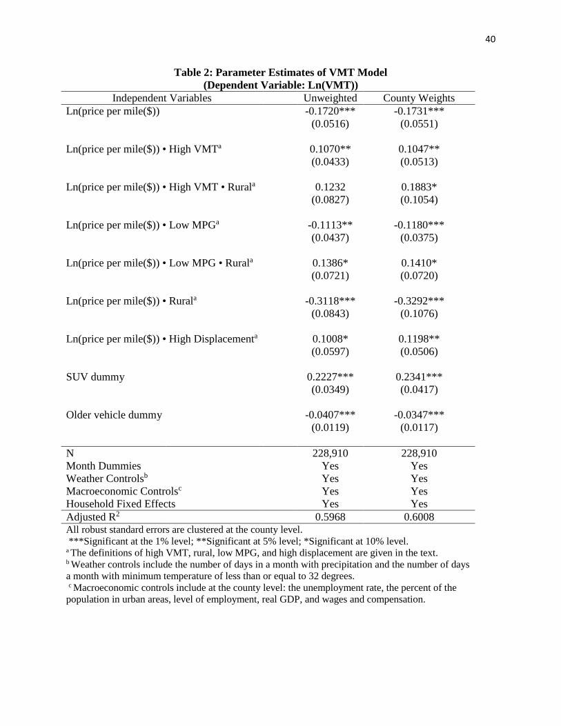
40

Table 2: Parameter Estimates of VMT Model

(Dependent Variable: Ln(VMT))

Independent Variables Unweighted County Weights

Ln(price per mile($)) -0.1720*** -0.1731***

(0.0516) (0.0551)

Ln(price per mile($)) • High VMTa 0.1070** 0.1047**

(0.0433) (0.0513)

Ln(price per mile($)) • High VMT • Rurala 0.1232 0.1883*

(0.0827) (0.1054)

Ln(price per mile($)) • Low MPGa -0.1113** -0.1180***

(0.0437) (0.0375)

Ln(price per mile($)) • Low MPG • Rurala 0.1386* 0.1410*

(0.0721) (0.0720)

Ln(price per mile($)) • Rurala -0.3118*** -0.3292***

(0.0843) (0.1076)

Ln(price per mile($)) • High Displacementa 0.1008* 0.1198**

(0.0597) (0.0506)

SUV dummy 0.2227*** 0.2341***

(0.0349) (0.0417)

Older vehicle dummy -0.0407*** -0.0347***

(0.0119) (0.0117)

N 228,910 228,910

Month Dummies Yes Yes

Weather Controlsb Yes Yes

Macroeconomic Controlsc Yes Yes

Household Fixed Effects Yes Yes

Adjusted R2 0.5968 0.6008 All robust standard errors are clustered at the county level.

***Significant at the 1% level; **Significant at 5% level; *Significant at 10% level. a The definitions of high VMT, rural, low MPG, and high displacement are given in the text. b Weather controls include the number of days in a month with precipitation and the number of days

a month with minimum temperature of less than or equal to 32 degrees.

c Macroeconomic controls include at the county level: the unemployment rate, the percent of the

population in urban areas, level of employment, real GDP, and wages and compensation.

41

Table 3 Annual Net Benefits ($2013) From a Gasoline Tax and VMT Tax to Reduce Fuel

Consumption 1%

31.2 cent/gallon gas tax 1.536 cent/mile VMT tax

Effect on:

VMT (billion miles) -29.5 -30.6

Consumer Surplus ($billions) -42.4 -42.9

Government Revenues ($billions) 42.2 42.7

Congestion ($billions) -2.84 -2.94

CO2 ($billions) -0.56 -0.57

Accident ($billions) -1.61 -1.67

Local Air Pollution ($billions) -0.35 -0.36

Total External Costs ($billions) -5.4 -5.5

Net Benefits ($billions) 5.1 5.3

Source: Authors’ calculations. Some columns may not sum precisely due to rounding. Total

external costs include a government service externality and a local air pollution externality in

addition to the congestion, accident, and CO2 externalities listed.

Table 4 Annual Net Benefits ($2013) From a Gasoline Tax and VMT Tax To Raise $55

billion Per Year For Highway Spending

40.8 cent/gallon gas tax 1.99 cent/mile VMT tax

Effect on:

VMT (billion miles) -38.0 -39.1

Consumer Surplus ($billions) -55.4 -55.5

Government Revenues ($billions) 55.0 55.2

Congestion ($billions) -3.66 -3.76

CO2 ($billions) -0.73 -0.72

Accidents ($billions) -2.07 -2.13

Local Air Pollution ($billions) -0.45 -0.46

Total External costs ($billions) -6.9 -7.1

Net Benefits ($billions) 6.5 6.7

Source: Authors’ calculations. Some columns may not sum precisely due to rounding. Total

external costs include a government service externality and a local air pollution externality in

addition to the congestion, accident, and CO2 externalities listed.

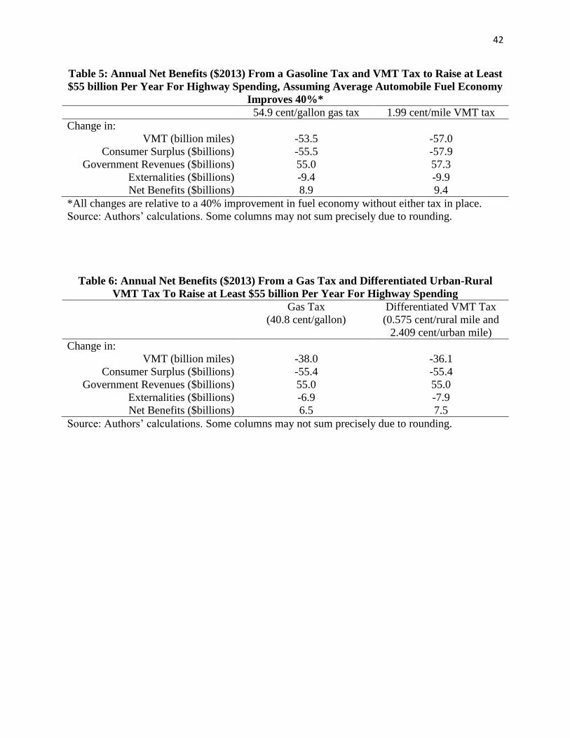
42

Table 5: Annual Net Benefits ($2013) From a Gasoline Tax and VMT Tax to Raise at Least

$55 billion Per Year For Highway Spending, Assuming Average Automobile Fuel Economy

Improves 40%*

54.9 cent/gallon gas tax 1.99 cent/mile VMT tax

Change in:

VMT (billion miles) -53.5 -57.0

Consumer Surplus ($billions) -55.5 -57.9

Government Revenues ($billions) 55.0 57.3

Externalities ($billions) -9.4 -9.9

Net Benefits ($billions) 8.9 9.4

*All changes are relative to a 40% improvement in fuel economy without either tax in place.

Source: Authors’ calculations. Some columns may not sum precisely due to rounding.

Table 6: Annual Net Benefits ($2013) From a Gas Tax and Differentiated Urban-Rural

VMT Tax To Raise at Least $55 billion Per Year For Highway Spending

Gas Tax

(40.8 cent/gallon)

Differentiated VMT Tax

(0.575 cent/rural mile and

2.409 cent/urban mile)

Change in:

VMT (billion miles) -38.0 -36.1

Consumer Surplus ($billions) -55.4 -55.4

Government Revenues ($billions) 55.0 55.0

Externalities ($billions) -6.9 -7.9

Net Benefits ($billions) 6.5 7.5

Source: Authors’ calculations. Some columns may not sum precisely due to rounding.

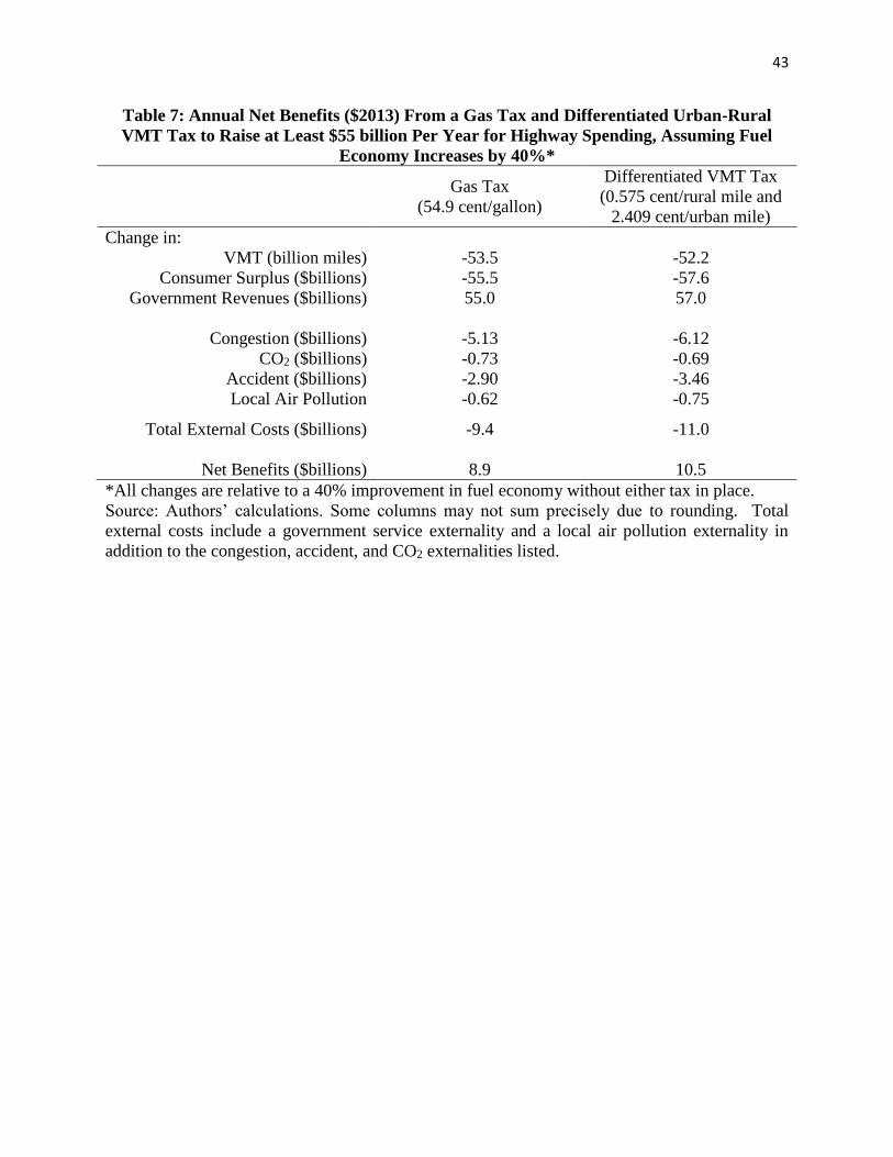
43

Table 7: Annual Net Benefits ($2013) From a Gas Tax and Differentiated Urban-Rural

VMT Tax to Raise at Least $55 billion Per Year for Highway Spending, Assuming Fuel

Economy Increases by 40%*

Gas Tax

(54.9 cent/gallon)

Differentiated VMT Tax

(0.575 cent/rural mile and

2.409 cent/urban mile)

Change in:

VMT (billion miles) -53.5 -52.2

Consumer Surplus ($billions) -55.5 -57.6

Government Revenues ($billions) 55.0 57.0

Congestion ($billions) -5.13 -6.12

CO2 ($billions) -0.73 -0.69

Accident ($billions) -2.90 -3.46

Local Air Pollution -0.62 -0.75

Total External Costs ($billions) -9.4 -11.0

Net Benefits ($billions) 8.9 10.5

*All changes are relative to a 40% improvement in fuel economy without either tax in place.

Source: Authors’ calculations. Some columns may not sum precisely due to rounding. Total

external costs include a government service externality and a local air pollution externality in

addition to the congestion, accident, and CO2 externalities listed.

44

Driver/Vehicle

High MPG

Vehicle Low MPG

Vehicle

High

VMT

High

VMT

Low

VMT Low

VMT

High 𝜖: VMT

tax increases

welfare much

more than a

gas tax. Low 𝜖: VMT

tax increases

welfare

somewhat

more than a

gas tax.

High 𝜖: VMT

tax increases

welfare

somewhat

more than a

gas tax. Low 𝜖: VMT

tax increases

welfare

slightly more

than a gas

tax.

High 𝜖: Gas

tax increases

welfare much

more than a

VMT tax. Low 𝜖: Gas

tax increases

welfare

somewhat

more than a

VMT tax.

High 𝜖: Gas

tax increases

welfare

somewhat

more than a

VMT tax. Low 𝜖: Gas

tax increases

welfare

slightly more

than a VMT

tax.

The welfare gain from a VMT tax is greater

than the welfare gain from a gas tax if the

total mileage response of vehicles that have

high fuel economy (MPG) is large. This

occurs if high MPG drivers have high initial

VMT and high gasoline price elasticities.

The welfare gain from a gas tax is greater

than the welfare gain from a VMT tax if the

total mileage response of vehicles that have

low fuel economy (MPG) is large. This

occurs if low MPG drivers have high initial

VMT and high gasoline price elasticities.

Summary Summary

Figure 1. Comparative Welfare Effects of a Gasoline and VMT tax for

Different Types of Drivers and Vehicles

45

Figure 2. Comparative Distributional Effects of a Gasoline Tax and a

Differentiated VMT Tax

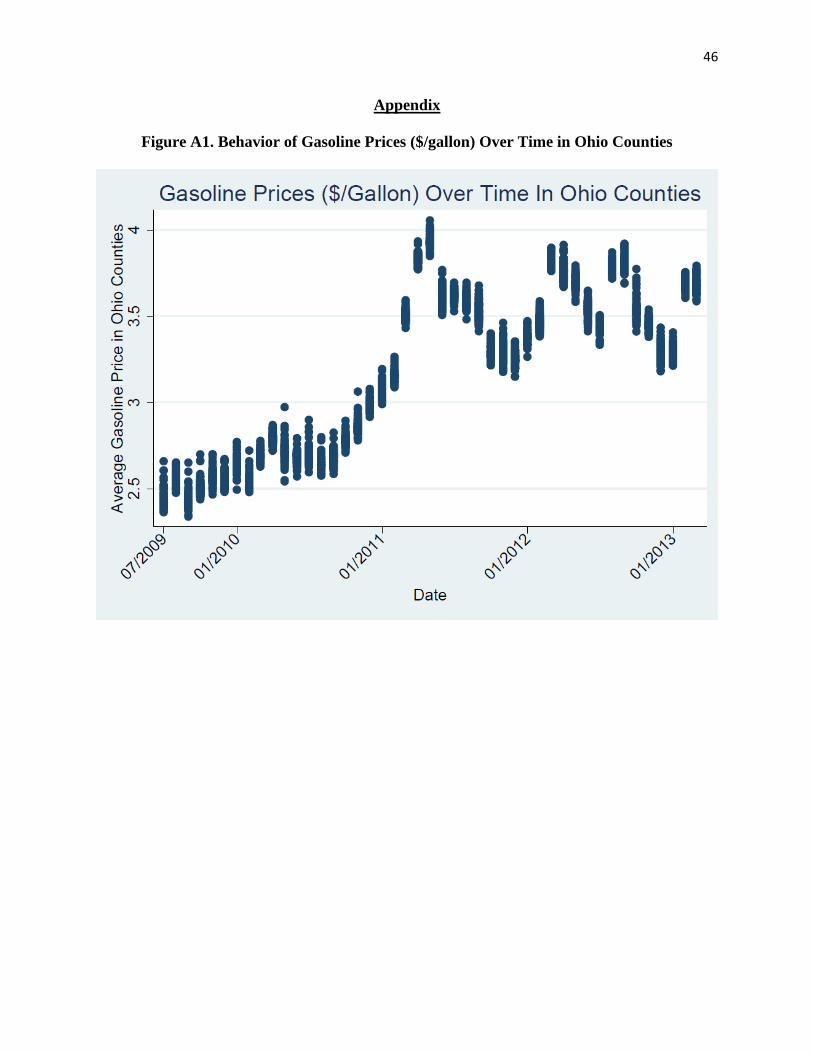
46

Appendix

Figure A1. Behavior of Gasoline Prices ($/gallon) Over Time in Ohio Counties