from humans to humanoids: a study on optimal ... - iit.it
TRANSCRIPT

Universita’ degli Studi di GenovaDipartimento di Informatica, Sistemistica e Telematica
Istituto Italiano di TecnologiaDipartimento di Robotica, Scienze Cognitive e del Cervello
From humans to humanoids: a studyon optimal motor control for the iCub
Serena Ivaldi
A thesis submitted for the degree ofPhilosophiæDoctor (PhD)
XXII Doctoral School on Humanoid TechnologiesApril 2011

Thesis supervisors:
Prof. Giorgio Metta (Principal Adviser)Robotics, Brain and Cognitive SciencesItalian Institute of Technology&Department of System, Communication and SciencesUniversity of Genova, Italy
Prof. Marco BagliettoDepartment of System, Communication and SciencesUniversity of Genova, Italy
Dr. Francesco NoriRobotics, Brain and Cognitive SciencesItalian Institute of Technology
This work has been carried out by Serena Ivaldi during her Ph.D. course in Humanoid tech-nologies, under the joint supervision of Prof. Giorgio Metta and Prof. Marco Baglietto, withthe additional supervision of Dr. Francesco Nori at the Robotics, Brain and Cognitive SciencesDepartment, Italian Institute of Technology, Genova, Italy, directed by Prof. Giulio Sandini.Her Ph.D. has been financially supported by the Italian Ministry of Education, University andResearch (MIUR), the Fondazione Istituto Italiano di Tecnologia (IIT), and by the EuropeanUnion through the projects ROBOTCUB, CHRIS, ITALK, VIACTORS.
Copyright © 2011 by Serena IvaldiAll rights reserved

1. Reviewer:
2. Reviewer:
3. Reviewer:
Day of the defense:
Signature from head of PhD committee:

If you don’t fail at least 90 percent of the time, you’re not aiming high enough.Alan Kay

Acknowledgments
There are many people without whom this thesis would not havebeen possible, and to whom Iam greatly indebted.I am obliged to my supervisors for guiding me through this difficult but exciting experience inresearch, and to Professor Sandini, who gave me the opportunity to join RBCS and work insuch a great research laboratory in IIT. I must thank Giorgiofor his sage advice. A specialacknowledgment to Riccardo and Olivier for reading the manuscript. My deepest gratitudeand appreciation goes to Francesco, whose teaching, guidance and friendship have been in-valuable in many senses, and a source of inspiration. If onlywe had worked together before.A special acknowledgment to my lab mates, theiCubers, colleagues and friends whom I havehad the pleasure to work with and spent most of the time in the last years, and particularly toAlessandra, Valentina, Monica, Elisa and Ambra, who have been friends more than colleagues.There are many people I should name at this point: either if you shared with me a single mo-ment of my PhD or many, thank you.I must thank my family, my sister, my friends, for loving and supporting me during these years.I hope they will be proud of me.Finally, I will never stop being grateful to Paolo for his love, patient encouragement and sup-port, for staying with me, and still being engaged to me despite my time being absorbed bystudy and work. This thesis is undoubtedly dedicated to him.

To Paolo

i

Glossary
CNS Central Nervous SystemEMG Electro-Myo-Graphy/icCPG Central Pattern generatorsM(A)JM Minimum (Angle) Jerk ModelM(C)TCM Minimum (Commanded) Torque Change ModelMVT Minimum Variance TheoryCA Cognitive Architecture
ERIM Extended RItz Method(N)MPC (Nonlinear) Model Predictive ControlDP Dynamic ProgrammingLQ(G) Linear Quadratic (Gaussian)DM Decision MakersOHL One-Hidden-Layer(A)NN (Artificial) Neural NetworksSVM Support Vector Machines(N)MSE (Normalized) Mean Squared ErrorCE(P) Certainty Equivalence (Principle)FH Finite HorizonRH Receding HorizonIH Infinite HorizonCOD Curse Of Dimensionality
DOF Degrees Of FreedomIK Inverse KinematicsFD Forward DynamicsCLIK Closed Loop Inverse KinematicsCOM Center Of MassEOG Enhanced Oriented GraphRNE(A) Recursive Newton-Euler (Algorithm)FT(S) Force/Torque (Sensor)OS Operating SystemIDE Integrated Development EnvironmentAPI Application Program InterfacePCB Printed Circuit BoardDSP Digital Signal Processing(L)GPL (Lesser) General Public LicenseCAD Computer Aided Design

Synopsis
Robots are going to coexist and interact with humans, sharing the same unstructured environ-ment and cooperating with them in many daily tasks. Even though industrial robots can achieveimpressive performances in terms of precision, relying basically on joint position controllersand classical control theory, there is now a wide consensus that such controls are not adequatefor the next generation of robots. More specifically, motioncontrol must be improved, with atwofold aim:
• imitating humans to produce more natural and possibly efficient behaviors;• guaranteeing motion safety.
My research stems from these considerations. In particular, I investigated motion control forthe upper limbs of a humanoid robot, focusing on the most important primitive for any ma-nipulation skill, i.e. reaching, taking inspiration from humans. Indeed, computational motorcontrol provides different models describing human motions, that can be used in the attemptof transferring such criteria on robotic platforms. I concentrated on a theoretical frameworkwhich allows describing the reaching problem as the result of an optimization process, wherethe success in reaching the target is not the only important parameter (i.e. bringing the end-effector of a manipulator on the target configuration) but also how the limb moves in effectingsuch actions, i.e. the criteria which can be used to describeits action. If we see this as anoptimization problem, then a stochastic functional optimization problem, with a suitable costfunction, state equation and constraints must be designed.Because the solution of functionaloptimization problems is almost impossiblea priori in real-time, an approximation techniquecombined with model predictive control has been addressed,where the solution to such prob-lems is explicitly precomputed via numerical techniques. Various simulations and experimentson a humanoid platform confirmed the feasibility of the proposed approach. Subsequently,I focused on the implementation of a theoretical framework that allows estimating joint tor-ques and external wrenches, under suitable hypotheses, fora wide class of robotic systems,and in particular for humanoids robots. The purpose was to provide a robot a force/torquecontrol framework which, combined with the optimization techniques, would enable human-like movements with active compliance. Experimental results successfully demonstrated thepossibility of controlling a complex humanoid robot in a compliant way. This lead to further in-vestigations regarding how to transfer human strategies invarying stiffness and torques duringpoint-to-point movements, using stochastic optimal control strategies. Although some activi-ties related to this topic are still work in progress, preliminary results favor the application ofsuch techniques, suggesting interesting developments.
iii


Contents
Glossary ii
Synopsis iii
1 Introduction 1
2 The robotic platforms 72.1 The humanoid robot James . . . . . . . . . . . . . . . . . . . . . . . . . . .. . . 72.2 The humanoid robot iCub . . . . . . . . . . . . . . . . . . . . . . . . . . . .. . . 10
3 Optimality: from humans to humanoids 173.1 Optimality principles in human motor control . . . . . . . . .. . . . . . . . . . . 19
3.1.1 CNS and motor control . . . . . . . . . . . . . . . . . . . . . . . . . . . .203.1.2 Learning, adaptation and re-optimization . . . . . . . . .. . . . . . . . . 213.1.3 Feedback and feedforward . . . . . . . . . . . . . . . . . . . . . . . .. . 233.1.4 Internal models . . . . . . . . . . . . . . . . . . . . . . . . . . . . . . . .263.1.5 Optimality and movement duration . . . . . . . . . . . . . . . . .. . . . 263.1.6 Optimality and locomotion . . . . . . . . . . . . . . . . . . . . . . .. . . 28
3.2 Which is the correct “cost function”? . . . . . . . . . . . . . . . .. . . . . . . . . 283.2.1 Minimum jerk . . . . . . . . . . . . . . . . . . . . . . . . . . . . . . . . . 293.2.2 Minimum torque change . . . . . . . . . . . . . . . . . . . . . . . . . . .303.2.3 Minimum variance . . . . . . . . . . . . . . . . . . . . . . . . . . . . . . 313.2.4 The Inactivation Principle . . . . . . . . . . . . . . . . . . . . . .. . . . 313.2.5 Which cost function? . . . . . . . . . . . . . . . . . . . . . . . . . . . .. 33
3.3 Optimality: from humans to humanoids . . . . . . . . . . . . . . . .. . . . . . . 343.3.1 Some implementations of optimal control models in robots . . . . . . . 363.3.2 Computational limits . . . . . . . . . . . . . . . . . . . . . . . . . . .. . 383.3.3 A layered control scheme . . . . . . . . . . . . . . . . . . . . . . . . .. . 393.3.4 Orchestration in a control scheme: team theory . . . . . .. . . . . . . . 40
4 Optimal control by means of functional approximators 434.1 Planning “optimally” goal-directed movements . . . . . . .. . . . . . . . . . . . 434.2 From functional optimization to nonlinear programming. . . . . . . . . . . . . . 48
4.2.1 Stochastic functional optimization problems . . . . . .. . . . . . . . . . 48
v

4.2.2 The Extended RItz Method (ERIM) . . . . . . . . . . . . . . . . . . .. . 514.2.3 A stochastic approximation technique . . . . . . . . . . . . .. . . . . . . 574.2.4 Team functional optimization problems . . . . . . . . . . . .. . . . . . . 604.2.5 Some notes on the optimization phase . . . . . . . . . . . . . . .. . . . . 61
4.3 Finite and Receding Horizon control problems . . . . . . . . .. . . . . . . . . . 634.3.1 Applying the ERIM to solve aT -stage stochastic optimal control problem 634.3.2 Variations in Finite Horizon problems . . . . . . . . . . . . .. . . . . . . 714.3.3 A Receding Horizon technique . . . . . . . . . . . . . . . . . . . . .. . . 75
4.4 Neural Finite and Receding Horizon regulators for reaching and tracking . . . . 844.5 Numerical results . . . . . . . . . . . . . . . . . . . . . . . . . . . . . . . .. . . . 87
4.5.1 A two DOF manipulator in a planar space . . . . . . . . . . . . . .. . . 884.5.2 A three DOF nonholonomic mobile robot in a planar space. . . . . . . 924.5.3 A two DOF arm actuated by elastic joints . . . . . . . . . . . . .. . . . 1004.5.4 Discussion of methods and results . . . . . . . . . . . . . . . . .. . . . . 101
5 Motion control on humanoids 1115.1 A closed loop control scheme . . . . . . . . . . . . . . . . . . . . . . . .. . . . . 1115.2 Closed Loop Inverse Kinematics . . . . . . . . . . . . . . . . . . . . .. . . . . . 1135.3 Forward Dynamics . . . . . . . . . . . . . . . . . . . . . . . . . . . . . . . . .. . 116
5.3.1 Robot dynamics: model or learning? . . . . . . . . . . . . . . . .. . . . 1175.4 Force/Torque feedback for control . . . . . . . . . . . . . . . . . .. . . . . . . . 121
5.4.1 Wrench transformations and FTS measurements . . . . . . .. . . . . . . 1245.4.2 Enhanced Oriented Graphs . . . . . . . . . . . . . . . . . . . . . . . .. . 126
5.5 Experimental results . . . . . . . . . . . . . . . . . . . . . . . . . . . . .. . . . . 1405.5.1 Closed loop motion planning with joint velocity control in James . . . . 1415.5.2 Estimation of intrinsic and extrinsic wrenches in iCub . . . . . . . . . . 1485.5.3 Joint impedance control of the iCub elbow . . . . . . . . . . .. . . . . . 160
6 Conclusions 167
Publications 171
References 172

Chapter 1
Introduction
It is a common belief that the human body movesoptimally and that human movements aregrounded on feedback and feedforward control processes [Todorov and Jordan, 2002]. Humanlimbs trajectories during goal-directed movements can be modeled by the optimization of aproperly defined cost functional, usually nonlinear and sometimes non-differentiable, subjectto sets of linear and nonlinear constraints [Biess et al., 2006, Berret et al., 2008].
In the literature different computational models can be found, describing trajectories interms of minimization of variance [Harris and Wolpert, 1998], torque change [Uno et al., 1989],jerk [Flash and Hogan, 1985], energy of moto-neurons signals [Guigon et al., 2008], etc.
In humanoid robotics, where reaching is the fundamental action primitive, such modelsare particularly of interest [Richardson and Flash, 2000],because they do not focus only on thesuccessful reach, but also on the trajectory performed by limbs, and the controls that cause theseactions. Through the implementation of such computationalmodels on robotic platforms it ispossible to mimic human movements and achieve, within certain approximations, human-likebehaviors. The crucial point is not to reproduce human behaviors to make the robot appearingmore human-like or natural [Seki and Tadakuma, 2004] but to achieve efficient control and tounderstand which principles governing the human body can betransferred on a robotic plat-form, assuming that the human body is the optimal reference,refined by evolution and years ofconstant learning and improvement [Atkeson et al., 2000, Shadmehr and Wise, 2005]. Analo-gous reasons explain why optimal control is frequently addressed to solve complex problemslike robot stabilization and walking [Lockhart and Ting, 2007, Atkeson and Stephens, 2007,Schultz and Mombaur, 2010, Mombaur et al., 2010].
In this perspective, the robot must be provided with a tool that is able to plan “optimally”: ifthe biological principles describing its motion are known,it must be able to generate proper tra-jectories and execute desired motions in real-time (possibly without being too much resource-demanding) with a suitable control scheme [Mitrovic et al.,2010].
Unfortunately, implementations on humanoid platforms face computational limits, sincemost optimal control problems incur in the Curse Of Dimensionality (COD), and even the solu-tion of simplified problems (e.g., after strong hypotheses reducing the complexity of the model)cannot always guarantee the fulfillment of time constraints[Diehl et al., 2009]. Rather thansearching for a generalized solution to the planning problem, whose computational limits make
1
it unsuitable for online real-time control, approaches in the literature usually focus on the opti-mization of single point-to-point movements [Simmons and Demiris, 2005, Matsui et al., 2006,Seki and Tadakuma, 2004, Tuan et al., 2008].
The corresponding optimal control problems are tackled vianumerical methods and non-linear programming algorithms, but the optimization process requires heavy computations andoften prevents the application in real-time. Since closed-form solutions are utterly hard to find(impossible in many cases) approximate solutions have to beconsidered.
Among the possible options, in this thesis an off-line approximation of the global con-trol law is preferred: the complete precomputation of a neural approximation of an explicitFinite/Receding Horizon (FH/RH) optimal control law (supported by an intermediate controlloop to compensate modeling errors) allows finding the controls almost instantly, leaving themachine free for other tasks during on-line execution (e.g.contact detection, learning, etc.)[Ivaldi et al., 2009b]. The proposed solution is globally only suboptimal, and locally optimal.
More specifically, the technique consists of two steps. In the first, off-line, a suitable se-quence of approximating functions is trained, so that they can approximate the sequence ofoptimal control functions of a stochastic Finite Horizon problem. The ERIM is chosen as afunctional approximation technique, while the use of feed-forward neural networks guaranteesthat the optimal solutions can be approximated at any desired degree of accuracy [Barron, 1993,Zoppoli et al., 2002, Kurkova and Sanguineti, 2005]. In theon-line phase, a single forwardcomputation of a neural network (consisting of few elementary operations) yields the propercontrol at each time instant.
Note that conventional Nonlinear Model Predictive Controltechniques such as FH/RHusually solve single instances of optimization problems, i.e. each trajectory is the result ofan optimization problem (typically varying its boundary conditions); conversely, in the pro-posed approach a generalized solution is found, for all the possible initial/desired conditions.The generalization is possible by combining functional approximation with stochastic optimalcontrol. Thus, in the on-line phase no further processing isrequired; the computation of theon-line controls is very fast, consisting only in the evaluation of a functional approximator;real-time performances can be guaranteed; furthermore, the machine controlling the robot doesnot require an external optimization routine (usually resource consuming), or licensed software,nor specific hardware.
The feasibility of this approach has been empirically demonstrated for the control of dif-ferent linear and nonlinear systems, such as a nonholonomicmobile robot [Ivaldi et al., 2008c]and planar manipulator; numerical results showing its effectiveness for different cost functionshave been presented in [Ivaldi et al., 2008a].
For humanoids, planning can be carried out either in the taskor directly in the robot jointspace. In the former case, the optimal trajectories can be converted into suitable –joint level–motor commands, exploiting suitable kinematics or dynamics control layers. If Cartesian spaceis used, for example, and joint velocity or position commands are used to control the robotmotion, one can use a classical closed-loop inverse kinematics algorithm (CLIK) for make the“task to space conversion”, taking into account the manipulator physical limitations. By tuningthe CLIK parameters (regulator, regularized Jacobian pseudo-inverse, etc.) it is possible toachieve great precision and stability in tracking the desired trajectory.
2

1. Introduction
But, if robots are going to coexist with humans, sharing the same unstructured environmentand interact with them and their objects, the capability to perform precisely a task must not sub-ordinate to the primary requirement of motion safety. Clearly, suitable force control schemesare necessary to address the tasks with compliance requirements and to guarantee the globalsafety during motion. An interesting analysis of the effects of uncontrolled impacts of roboticmanipulators on humans can be found in [Haddadin et al., 2008a, Haddadin et al., 2008b].
Classically, and especially in industrial environment, great effort has been focused on po-sition control rather than compliance and force control, because the application domain re-quired precise performances (which are normally achieved by stiff, high gain joint positionfeedback control). The lack of compliance has been traditionally compensated by collisionavoidance solutions, where commonly the end-effector trajectory or the manipulator configu-ration is changed during motion so as to avoid collisions with the surrounding (or the self). Theliterature in this topic is vast, and outside the scope of thethesis, but the interested reader canrefer to [Minguez et al., 2008, Kulic and Croft, 2007, Sisbotet al., 2010].
Recent developments in actuator technology have driven theattention towards systemscapable of intrinsic joint-torque control and more in general passive compliance: variableimpedance/variable stiffness actuators [Eiberger et al.,2010, Albu-Schaffer et al., 2010], se-ries elastic actuators [Pratt and Williamson, 1995], pneumatics and hydraulics actuators, etc.Though being intrinsically compliant and thus safer with respect to DC motors, elastic ele-ments combined with actuators do not guarantee safety, as they can store great amounts ofpotential energy, which once released can have greater impacts on both robot and environ-ment, as recently shown in [Haddadin et al., 2010a]. Moreover, these solution often requireconsistent mechanical re-design [Tsagarakis et al., 2009]and the adoption of different formsof power sources [Amundson et al., 2005].
An alternative approach isactive compliance, or active force, consisting in the regula-tion of the interaction forces at each instant of time by means of closed-loop force controllers[Sciavicco and Siciliano, 2005]. The principle being that if external forces can be detectedor measured with suitable sensors, they can be controlled soas to regulate the interactionforces to the desired value: thus, active force control strategies can be build [Mistry et al., 2010,Calinon et al., 2010, Fumagalli et al., 2010a]. The main advantage of the active regulation overthe passive one is the possibility of regulating forces within a wider range of values. One dis-advantage is the response delay of the regulator, which typically limits the bandwidth of thecontrolled system. This approach, given the model of the robot (such as rigid body dynamicsmodel), requires the hardware necessary to measure forces/torques (not only in joints, but atthe end-effectors and at any other possible contact point ofthe robot). Traditionally, the mostadopted solution consists in modifying the motor/joint group in order to insert suitable tor-que sensors, as was done in [Parmiggiani et al., 2009] to integrate joint-torque sensing in thefore-arm of the humanoid iCub, or redesign the robot to include torque sensing, as was donein [Luh et al., 1983] for a Stanford manipulator. As an alternative to placing joint torque sen-sors, an estimation of motor torques can be obtained from thecurrent absorbed by the motors(feasible only when most of the motor torque is transmitted to the joint – low friction).
Another approach consists in exploitingForce/Torque Sensors(FTS): FTS are relativelysmall and compact, and can be often inserted in the kinematicchain easily when the available
3

space on the robotic platform is limited and passive elements cannot be inserted without radicalchanges. In industrial applications, robots are typicallyequipped with FTS mounted at the end-effector, where the most interaction with the environment occurs. The solution described in thisthesis is based instead on a set ofproximalFTS, instead at the base of the kinematic chains andfar from the end-effectors: this configuration allows measuring not only interaction forces act-ing at the end of the chains, but also forces acting in betweenthe sensor and distal joints. A sim-ilar solution has been adopted only once in [Morel and Dubowsky, 1996, Morel et al., 2000]where a single FTS was used to estimate the joint torques in the first 3 Degrees Of Freedom(DOF) of a PUMA manipulator. Here, we propose a method which exploits sets of FTS placedproximally in a multi-branched chain to estimate joint torques of complex kinematic chains. Inparticular, given the FTS measurements, if a precise dynamical model of the robot is known(i.e. a rigid body model), internal forces and torques can becomputed easily by a classicalrecursive Newton-Euler method, and if suitable assumptions hold, certain external forces canbe also estimated. As prove of the effectiveness of this approach, we successfully estimate 32of the 53 DOF of a full-body humanoid robot.
The theoretical framework for computing simultaneously intrinsic torques and externalwrenches applied to single and multiple branches kinematicchains, is based on two funda-mentals:
• the Enhanced Oriented Graph (EOG), i.e. a graph representation of kinematic chains,enriched with symbols for representing unknowns and sensormeasurements;
• theRecursive Newton-Euler Algorithm (RNEA)for the computation of inverse dynamicsof fixed and floating base kinematics chains.
A systematic procedure for computingN + 1 external wrenches fromN internal wrenches(i.e. measurements from FTS) is also given, under certain assumptions. Remarkably, underthese conditions all joint torques can be theoretically computed. In order to compute externalwrenches, the main requirement is that their application point must be known: this informationcan be fixeda priori for particular robot tasks, but in general must be updated on-the-fly. Onthe platform used in this work – the iCub – it is provided by a set of tactile sensors, constitutinga sort of “artificial skin” [Cannata et al., 2008, Maggiali etal., 2008].
Experiments have been performed in a variety of floating baseconditions (e.g. standing,crawling) and with different interactions with the environment. Experimental observationsalso proved that controlling joint impedance in the robot isfundamental to obtain compliantinteraction with the environment and make the robot move in amore safe and natural way.Interestingly, the neural optimal controller has been effective in computing adaptive strategiesfor controlling stiffness and torque of elastic actuators during point to point movements. Al-though some experiments on the iCub are work in progress, preliminary results show that it ispossible to apply computational motor control models used to investigate human movementsonto robots, up to a certain extent, given the physical differences between the two systems.
4

1. Introduction
Contribution of this thesis
In this thesis two theoretical frameworks are proposed. Thefirst is a mathematical tool to im-plement stochastic optimal motion control on humanoid robots, which in a sense seeks inspira-tion from computational motor control models. The proposedmethod consists of a stochasticapproximation technique combined with a model predictive control scheme; intermediate con-trols, at joint level, are introduced to comply with the robot requirements. The second is atheoretical framework for computing the dynamics of a humanoid robot and estimate jointtorques and external wrenches. Notably, this tool enabled to create different interfaces for con-trolling the robot in a compliant way, particularly joint torque control and impedance control.For each of the above, C++ software libraries have been produced, the NeuBot and iDyn libraryrespectively. The latter has been released under GPL license as a part of the iCub Project, whilethe first is available upon request from the author.
The content of this thesis has been partially published as research papers. Their detailedreferences are reported in the bibliography section.
The thesis is organized as follows.In Chapter 2, the humanoid robots which have been used as experimental platforms are
described: James, a humanoid torso, and iCub, a fully body humanoid.In Chapter 3, the optimality principles used to describe motor control are presented. Start-
ing from a brief discussion on the experimental observations performed on humans, we overviewthe main computational motor control models which have or may have or might influence mo-tor control models in humanoids. Some successful examples of integration of optimal controlin robotics are presented, along with a discussion of the main differences between the two sys-tems, which sometimes prevent a straightforward application of neuro-computational modelsinto robots.
In Chapter 4, the reaching and tracking problem are introduced in the optimal controlframework, and the approximate solution via the ERIM, combined with NMPC is discussed.Some numerical results are discussed, pointing out the advantages and disadvantages of themethod, and particularly of the ERIM. However, its application to different problems, high-lights its ability to adapt to different contexts: deterministic, stochastic, with linear and nonlin-ear systems,etc.
In Chapter 5, the closed loop lower level controllers are discussed: first, the Inverse Kine-matics, secondly the force/torque control layer. Since theiCub is not provided with joint torquesensing, in Section 5.4 a framework for computing internal torques and external wrenches froma set of proximal FTS (available in the iCub) is presented. Finally, Section 5.5 reports someexperiments with the humanoid platforms.
Chapter 6 draws the conclusions and suggests future works.
5

6

Chapter 2
The robotic platforms
Two humanoid robotics platforms have been used to validate the theoretical results discussedin this thesis, and to assess the proposed methods with experimental results: the 22 DOF upper-torso James, and the 53 DOF full-body iCub. Experiments havebeen performed at the ItalianInstitute of Technology, where both robotics platforms areavailable.
(a) (b)
Figure 2.1: The humanoid robots James2.1(a)and iCub2.1(b).
2.1 The humanoid robot James
James [Jamone et al., 2006] is a 22 DOF torso (see Figure 2.1(a)), with the overall size of a 10years old boy and a total weight of about 8 kg. It has a head, with moving eyes and neck, a leftarm with a highly anthropomorphic hand.
The robot is actuated by 23 rotary DC motors (Faulhaber [Faulhaber, www]). Torque istransmitted to the joints by rubber toothed belts, pulleys and stainless-steel tendons. Cablespulling solutions have been particularly useful in designing the hand, since most of the hand
7

actuation have been located in the wrist and forearm rather than in the hand itself, where sizeand weight constraints would have limited the proliferation of DOF. Furthermore, tendon ac-tuation naturally provides certain compliance to the system. Extra compliance has been intro-duced by means of springs in series with tendons, for examplein fingers. The drawbacks ofelastic transmission are the nonlinear effects which reveal during rough movements (i.e. whencontrolling joints with high velocities).
Mechatronics of James
The head has two eyes (i.e. CCD digital cameras, Dragonfly) which can pan and tilt indepen-dently, for a total of 4 DOF. A 3-axis orientation tracker (Intersense iCube2) is mounted on thetop of the head, to emulate the vestibular system. The tracker, basically a gyroscope, providesan absolute measure of acceleration, velocity and positionwith respect to the Cartesian axesof a reference frame, thus it is also called inertial sensor.The head is mounted on a two DOFneck, consisting of a tendon driven rigid spring, which allows bending forward (pitch) and lat-erally (roll) [Nori et al., 2007a]. The actuation is obtained with a peculiar structure, recallingthe design of a tendon-driven parallel manipulator: in particular, three steel tendons, separatedby 120 degrees, are used to achieve the two motions. On the topof the neck, a custom-madeforce sensor with a cantilever beam structure is positioned, so as to provide force feedback tothe three motors actuating the neck [Fumagalli et al., 2009].
The arm has seven DOF: three in the shoulder, one for the elbowand three in the wrist. Inparticular, the shoulder consists of three rotative joints, actuated through tendons and pulleys bythree DC motors located in the torso: two joints (the ones yielding abduction) are mechanicallycoupled, as shown in Figure 2.2(a), so as to gather the shoulder a wider range of motion.Notably, thanks to this solution, James can perform wide range movements, for example itcan reach its torso, its right shoulder and drive its left armbehind the head: these cannot beperformed by even more recent humanoid robots, like iCub. Inthe middle of the upper arm, asingle ATI mini45 FTS [ATI, www] is located, as shown in Figure 2.2(b). When FT sensorsare added to a kinematic chain, they are usually placed on theend-effector, i.e. where mostinteraction occurs. In James the proximal location1 has been chosen as the remainder of thefree space in the upper and fore-arm was entirely occupied bythe motors actuating the wrist,elbow and fingers, and DSP boards used to control them. The benefit of this configurationis that the FTS is able to detect interactions with the environment occurring not only on theend-effector (e.g. a grasp) but on the whole arm (e.g. the elbow colliding with an object).This means also that there is not a predetermined contact point, or the whole arm surface is apossible contact point.
A highly anthropomorphic hand, designed for grasping purposes, is the end-effector ofthe manipulator. The hand has five fingers, actuated by eight motors, and a total of 17 DOF:each of the five fingers has three joints (extension of the distal, middle and proximal pha-lanxes), and two additional DOF account for the thumb opposition and by the coordinatedabduction/adduction of the other four fingers. Tactile information is provided by custom-madesensors, placed along the fingers and the hand palm. These sensors, constituted by a two part
1Proximal means far from the end-effector.
8

2. The robotic platforms
(a) (b)
Figure 2.2: 2.2(a). James shoulder (3 DOF). The picture shows the three DOF of the shoulder.Notice in particular how the yaw rotation is obtained by a double rotation around two parallel axes(image from [Jamone, 2010]).2.2(b) Detail of the upper-arm. The ATI Mini45 FT sensor (redsquare) is placed below the shoulder group.
silicone elastomer, a miniature Hall Effect sensor and magnet, have been designed specificallyfor James. More details on their design and application can be found in [Jamone et al., 2006,Jamone, 2010].
Hardware architecture for control
Motor control is distributed on eight Digital Signal Processing (DSP) boards (Freescale DSP-56F807, 80MHz, fixed point 16 bits [Freescale DSP, www]), which perform a fast low-levelcontrol loop (1KHz rate). A CAN-bus line allows the communication between the boardsand a remote PC, where an ESD CAN-USB is provided. The middleware and the inter-process communication is grounded on YARP [Metta et al., 2006]. Magnetic and incrementalencoders are used for the feedback position control loop implemented on the boards. Mostof the motors are directly controlled by standard PID controllers, except for the shoulder,neck and eyes motors which require different control strategies to handle various mechani-cal constraints. The available DSP boards have limited memory and computation capabilityand cannot support but simple operations, namely low level motor control (basically PID po-sition control), signal acquisition and pre-filtering fromthe optical encoders. For this reasons,implementing an on-line controller directly on the DSP boards is impossible in the currentsetup. Reference position and velocity commands can be set by the user through a stan-dard YARP port, communicating in the local network to the so-called “James Interface”: acollection of YARP threads and modules, which acts as a bridge between the device driversrunning on the boards and the remote PC. More accurate descriptions of the control archi-tecture and the different low level as well as high-level control strategies, can be found in[Jamone et al., 2006, Fumagalli et al., 2009, Nori et al., 2007a].
9

Figure 2.3: Some pictures of James’s arm moving in the space. Only shoulder and elbow jointsare controlled.
2.2 The humanoid robot iCub
The aim of the RobotCub consortium [RobotCub Project, www] has been the development ofan open-source infant-like robotic platform, aimed at reproducing the same motor and cognitiveabilities of a two years old child [Tsagarakis et al., 2007, Metta et al., 2010]. The iCub not onlyhas the shape of a human baby, but also a complex cognitive architecture reflecting the manyprocesses involved in the functional development [Sandiniet al., 2007, Vernon et al., 2007a,Vernon, 2010].
iCub is a 53 DOF full body humanoid robot, of the same size as a two-three years oldchild. It was designed to crawl on all fours, and sit up with free arms. The most of its DOFsare located in the upper-body, especially in the highly anthropomorphic hands, which allowdexterous and fine manipulation. It has comprehensively proprioceptive, visual, vestibular,auditory and haptic sensory capabilities.
Certain features of the iCub are unique. The peculiar aspectis that it is a completely opensystem platform: both hardware and software are licensed under the GNU General PublicLicense (GPL), and the middleware used for intra-process communication, YARP, is an open-system too, released under GNU Lesser General Public License (LGPL) [Metta et al., 2006].
Mechatronics of the iCub
The iCub is about104cm tall and weighs22kg, with a total of 53 DOF: six in the head (yaw,pitch, and roll in the neck, pan, tilt and vergence in the eyes), three in the torso (yaw, pitch, androll), seven in each arm (three in shoulder, one in the elbow and three in the wrist), six for eachleg (three in hip, one in the knee and two in the ankle), the remainder in the hands.
Actuation is provided by electric motors. The major joints are actuated by brushless DCmotors, coupled with harmonic drive gears, so that high torques (up to40Nm) are guaranteedfor the critical joints, such as hips, spine and shoulders. Head and hands are actuated by smallerDC motors. Most of the joints (e.g. in hands, shoulder, waist) are tendon-driven: this reducesthe size of the robot and also introduces a certain elasticity (which can be a drawback if precisecontrols with high velocities are addressed, an advantage for its intrinsic compliance if safetyis addressed).
The neck and the eyes are fully articulated (three DOF each),to support tracking and ver-gence behaviors.
Each hand (see Figure 2.6) has 5 fingers and 19 joints, and is actuated by 9 motors (sinceseveral joints are coupled). The first three fingers (thumb, index and middle finger) are in-
10

2. The robotic platforms
Figure 2.4: The humanoid iCub, fully covered by plastic shells, standing on a metallic mainstayover a mobile platform in the RBCS laboratory at IIT.
dependent and constitute eight DOF; while the fourth and fifth ones, used only for additionalsupport to grasping, are coupled and constitute one single DOF. The hands allow a considerabledexterity though being very small: the palm length is 50mm, 25mm thick; the total width of thehand range from 34 to 60 mm at wrist and fingers respectively. These features are quite uniquein humanoid robots with similar dimensions as iCub. This solution is possible because mostof the actuation is located in the forearm, and tendons are routed to the hand joints via a wristmechanism. Each joint is indeed tendon driven. The flexing ofthe fingers is directly controlledby the tendons, while the extension is based on a spring return mechanism (basically this savesone cable per finger).
The 7 DOF arm does not allow the same motion range as in James (e.g. iCub cannottouch its back) and additional physical constraints such asthe body covers prevent a completeexploitation of the robot workspace. To provide better flexibility for manipulation, a 3 DOFwaist has been incorporated, to increase the range of motionof the upper body, resulting ina larger workspace for manipulation. Finally, legs have been designed to support crawlingand sitting, but are also adequate for standing and walking.The ankle has two DOF, namelyflexion/extension and abduction/adduction (foot twist rotation was not implemented).
Additional sensing capabilities
Proprioception is provided at each joint by positional sensors, generally absolute position en-coders. Joints positions are then retrieved directly from encoders measurements, while joints
11

velocities and accelerations are derived from position measurements through a least-squares al-gorithm based on an adaptive window filter [Janabi-Sharifi etal., 2000, Fumagalli et al., 2010b].
Many other different devices enrich the sensory capabilities of the iCub: digital cameras(for the eyes), gyroscopes, microphones, accelerometers,tactile and force sensors.
The latter three set of sensors are fundamental for the iCub active compliance, as will bediscussed in Chapter 5. As shown in Figure 2.7(b) and 2.7(a),iCub is equipped with one inertialsensor (Xsens MTx-28A33G25 [Xsens, www]) located on the head, providing measurementsof linear acceleration and angular velocity and acceleration2. Four custom-made six-axes FTS(see Figure 2.8), one per leg and arm, are placed proximally with respect to the end-effectors(hands and feet).
Sets of distributed capacitive tactile sensing elements are integrated on most of the plasticshells covering the robot limbs [Cannata et al., 2008], and provide a tactile feedback for pos-sible contacts with the environment. This sort of “artificial skin” is constituted by a layer ofcapacitive pressure sensors included on a flexible Printed Circuit Board (PCB), with embeddedelectronics, covered by a silicone foam to protect each taxel (i.e. tactile element) and make theskin also more compliant. An example of the device for the forearm is shown in Figure 2.9.
Moreover, a set of fingertips, one per each finger, provides additional tactile information,for fine manipulation. The first prototype consisted of rectangular sensitive zones, made ofconductive ink painted on an inner support and connected to arigid PCB. The final device ismade of a capacitive pressure sensor, a flexible PCB layer with circular taxels, wrapped aroundthe inner support, and covered by layers of silicone foam andconductive rubber connected tothe ground [Schmitz et al., 2010].
Hardware architecture for control
A set of DSP-based control cards, custom designed to fit the limited space available in theiCub, takes care of the low-level control loop. Each controlboard runs at1 kHz, and is con-nected to the main relay CPU (a PC104, located in the robot head) via CAN bus (four linesin whole), which retrieves all motor-sensory information,handles synchronization and refor-matting of the various data streams. More demanding computation can be performed on aPC cluster connected to the PC104 via a Gigabit Ethernet. Additional electronics have beendesigned to sample and digitalizes the numerous sensors: also in this case, all the signals con-verge to the PC104 by means of additional connections (e.g. serial, firewire). Moreover, therobot is equipped with an umbilical cord containing both an Ethernet cable and power supplyline: with this solution, it can move freely in the space without being constrained to a specificposition. A simple scheme describing the hardware/software architecture for control is shownin Figure 2.10.
Software architecture
The core of the iCub software architecture is a set of modulesdeveloped on top of YARP[Metta et al., 2006, Fitzpatrick et al., 2008]. YARP is a set of cross-platform C++ libraries,
2Precisely, angular acceleration is found using an adaptivewindow filter.
12

2. The robotic platforms
which supports modularity, and provides universal interfaces with hardware and device mod-ules. The philosophy is code reuse, which is to wrap each native device API, and provide asimple generic interface for any hardware device, so that changes in the hardware do not implyrewriting all modules, but only changing the API calls. Moreover, YARP is independent fromboth operating system and development environment, thanksto ACE and CMake: the firstis an OS-independent library for inter-process communication, the second a cross-platformmake-like tool to generate platform and IDE specific projectfiles.
In the YARP framework, a suitable real-time layer is in charge of the low-level control ofthe robot, namely a set of processes running on the boards located through the robot body, inter-facing sensors and actuators with the PC104. A pool of YARP modules defines a soft real-timecommunication layer, when multiple processes can coexist and exchange data through a se-ries of universal ports, following the observer pattern by decoupling producers and consumers.This architecture is evidently suited for cluster computation: each module can be called orobserved remotely from within the network. One evident drawback is that this architecture nat-urally excludes direct real-time control (i.e. a module directly sending commands to the joints),because of the many layers interposed in between the controller module (typically a modulerunning on a cluster PC) and the robot hardware. Issues related to real-time performances mustbe addressed elsewhere.
13

(a)
(b)
Figure 2.5: Top (2.5(a)): some snapshots of the “Yoga” demo, where iCub perform periodically aset of pre-programmed movements in the space. The base frameis fixed, being iCub supported bya metallic mainstay.Bottom (2.5(b)): some snapshots of iCub crawling on a carpet. Black strapsare used to protect knees and wrists and simultaneously improve the friction of the plastic coverswith the floor. Limbs motion is orchestrated by a controller based on central pattern generators[Degallier et al., 2008]. Self-body collision is preventeda priori. Interaction with the environmentoccurs on knees and wrists. The base frame is floating.
Figure 2.6: The iCub hand: in evidence, the embedded electronics (a MAISboard on thetop), the tactile skin covering the palm and the tactile fingertips. More details can be found in[Schmitz et al., 2010].
14

2. The robotic platforms
(a) (b)
Figure 2.7: Right (2.7(a)): the force/torque and inertial sensors used in iCub.Left (2.7(b)): amechanical scheme of the humanoid robot iCub: in evidence, the four proximal six-axes FTS (legsand arms) and the inertial sensor (head).
Figure 2.8: The custom FTS developed for iCub. Left: the sensing element. Center: the embeddedelectronics. Right: the assembled sensor. Notice the CAN line, going out from the sensor, whichtransmit sampled digital measures at1ms rate (image from [Fumagalli et al., 2010b]).
15

Figure 2.9: Distributed tactile elements constitute a sort of artificial “skin”. The plastic cover, theelements and the final device for the fore-arm are shown. Details about skin fabrication and howiCub has been covered with it can be found in [Roboskin Project, www].
Gb
Eth
ern
et
8 C
AN
bu
s lin
es
(1M
bp
s)
PC 104
iCubInterface
RobotMotorGui
WholeBodyTorqueObserver
Inertial Sensor
Force/Torque Sensors
DSP boards
COM
Motion Planning
Figure 2.10: A scheme showing the networked control infrastructure. ThePC104 collectsjoints measurements from the DSP boards, inertial measuresfrom a specific COM port, andFTS measures via CAN bus. Each FTS is equipped with embedded electronics, with A/D con-verters. Through the iCubInterface, all measurements are replicated in the YARP local net-work, where a PC cluster is available, and multiple processes coexist. Among these, one isdedicated to the computation of “virtual” joint torques (asdescribed in Section 5.4), one tothe selection of the control modality (e.g. joint position,velocity or torque control). Theestimated torques are sent back via the PC104 to the DSP boards to enable torque feed-back. More details on this scheme can be found in the online documentation of the iCub:http://eris.liralab.it/wiki/Force Control.
16

Chapter 3
Optimality: from humans tohumanoids
Novel trends in computational neuroscience suggest that optimal control theory is crucial tounderstand the motor commands and the motor control that thehuman exerts during a task.Many researchers support the theory that the motions we observe in humans and animals are“optimal”, because the sensorimotor system is the product of millions of years of evolution,but also because it constantly “evolves” being subject to continuous process such as learning,adaptation and training, which improve behavioral performance in terms of stability, accuracyand efficiency [Shadmehr and Wise, 2005, Franklin et al., 2008]. Even if the physical structureof the human body precludes certain motions, among a wide variety of possibilities, the CNSchooses to implement a selected set of planning strategies.We will consider these movements(that we can observe everyday) as “optimal”, with the meaning that optimal control is a goodmodeling tool for human motor control. The idea that a motor controller is not only adaptive,but also optimal, suggests statingthe motor problem as a stochastic optimal control problem.
It is a common assumption that the motions we observe in humans and animals are “opti-mal”, because the sensorimotor system is the product of millions of years of evolution, but alsobecause it constantly “evolves” being subject to continuous process such as learning, adapta-tion and training, which improve behavioral performance interms of stability, accuracy andefficiency [Shadmehr and Wise, 2005, Franklin et al., 2008].Even if the physical structure ofthe human body precludes certain motions, among a wide variety of possibilities, the CNSchooses to implement a selected set of planning strategies,leading to the “optimal” arm move-ments that we can observe every day.
Stochastic optimal control theory might provide the important link across the three lev-els of motor system: motor behavior, limb mechanics and neural control [Todorov, 2005,Todorov and Jordan, 2002, Todorov, 2004]. It naturally provides a mathematical frameworkto explain which are the controls generating the observed behavior, by providing or exploitinga cost function to describe the motion criteria.
Moreover [Scott, 2004], it might help to unravel how the primary motor cortex and otherregions of the brain plan and control movement, providing valuable insights into the adaptivetask-dependent control of movements. For this reason, neuroscientists and engineers cooperate
17

Figure 3.1: Optimal feedback control as the neural basis for motor control. The basic principleis that feedback gains are optimized on the basis of some index of performance. Such controllerscorrect variations (errors) if they influence the goal of thetask; otherwise, they are ignored. Optimalstate estimation is created by combining feedback signals and efferent copy of motor commands.The latter uses a forward internal model to convert motor commands to state variables (image from[Scott, 2004]).
for identifying the possible one-to-one correspondences between CNS and control schemes.In general, all models agree on a certain control scheme, where the body (limbs, muscles,
etc.) is the plant to control, the optimal controller provides feedback, sometimes feedforwardterms, relying on an internal model of body and environment,while delayed signals are fedto a state estimator. The corresponding conceptual scheme,in one possible representation, isshown in Figure 3.1. A more detailed scheme is shown in Figure3.2.
Concerning the optimal controller, two principal approaches can be used to select or iden-tify a motion criteria. The first is to exploitinverse optimal control theory[Dupree et al., 2009,Krstic, 2009]: after recording experimental data, trying to infer the cost function to which theobserved behaviors are optimal. The second, which is actually the most used, is to choose a pri-ori a sound cost function and a mathematical model, and to verify its effectiveness in capturingthe motion principles by comparing model predictions with experimental observations.
However, it is still uncertain how the CNS determines such optimal control policies. Mo-tor control and learning explain the exceptional dexterityand rapid adaption to changes, whichcharacterize human motor control, but do not provide an unique answer to the questions regard-ing the criteria which are at the basis of such plasticity anddexterity. So far, many differentcomputational models have been proposed.
Existing optimization principles can be divided into two groups:
1. Deterministic approaches, where the cost is typically expressed as the integral of somedeterministic function over the movement time. The problemis stated as the minimiza-tion of the cost subject to a set of dynamic constraints and boundary conditions.
• Minimum jerk model [Flash and Hogan, 1985]• Minimum torque change model [Nakano et al., 1999]
2. Stochastic approaches, where random disturbances are included in the description of themodel, thus the expected value of the cost function, subjectto dynamic constraints and
18

3. Optimality: from humans to humanoids
Figure 3.2: A schematic model for generating goal directed movements. With specific referenceto the model proposed by Shadmehr and Krakauer, the cost/reward function refers to basal ganglia,the state estimation is performed by the parietal cortex, while the forward model can be put downto the cerebellum. The feedback controller is actually a combination of different modules whichcan be referred to the premotor and motor cortex (image from [Shadmehr and Wise, 2005]).
boundary conditions, can be minimized.
• Minimum variance model [Harris and Wolpert, 1998]• Minimum intervention model [Todorov and Jordan, 2002]
In the following we will overview the main basic principles of human motor control whichcan be considered as “optimal”, and focus on some computational models which have beendeveloped to model goal directed movements. However, the question “which is the cost func-tion?” will remain unanswered. We will then discuss our views on trying to transfer the conceptof optimality from humans to humanoids, trying to identify the challenges and introducing themethod we propose in this work, which will be object of the next chapter.
3.1 Optimality principles in human motor control
Human movements in adults show several prominent features.Multi-joint arm trajectories fordiscrete point-to-point planar movements, for example, have some spatiotemporal invariantfeatures: roughly straight hand paths, bell-shaped velocity profiles and smooth acceleration[Morasso, 1983, Flash and Hogan, 1985, Kelso, 1982].
These invariant features can be seen as the result of an twofold optimization process: onecoming from the CNS, evolved in time since the origin of our species, one from the personalontogenesis process, where movements are refined. Even if the latter should yield in eachperson a certain variability to the motor trajectories, experimental results bring evidence thatbehaviors in human motor control are basically stereotyped.
Despite the huge number of possible combinations of agonistic and antagonistic muscletensions that can generate the same torque, and the intrinsic noise of the motor system, ob-served hand trajectories are stereotyped, and the EMG signals show a typical triphasic pattern
19

activation. Clearly, the motor control system solves such infinite-dimensional problems ac-cording to some principles.
In the following, we will briefly describe the CNS, i.e. the biological structure in chargefor motor control, and some insights on the learning and adaptation mechanisms which makethe primate rough infant movements evolve to adult ones. Then, a review of the main computa-tional motor control models, which can be of interest for robotic applications, is presented anddiscussed.
3.1.1 CNS and motor control
The CNS we study nowadays is the product of millions years of evolution, it is worth ananalysis since it can provide some insights for a human inspired motor controller .
The CNS is a complex system which allows us to move, acquire skills, and adapt thoseskills to a variety of contexts. Each time we reach for an object, the CNS must solve a com-plex physical problem, to control and coordinate our limbs during interaction with a changingenvironment, subject to gravity [Shadmehr and Wise, 2005].
It consists of two major parts: the spinal cord and the brain,composed by the brainstem,divided into forebrain, midbrain and hindbrain (in its turndivided into medulla and pons). Alllevels of the CNS participate in motor control and motor learning, and in primates they allcontribute to visually grounded reaching and pointing.
The forebrain, consisting of diencephalon and telencephalon, contains several structuresthat play a role in motor control. The hypothalamus, which isthe main controller for the bodyfunctionalities, including homeostasis, reproduction and defense. The basal ganglia, receivingan efference copy of the motor commands, and providing an internal model of the body1. Thethalamus, integrating the distributed brain systems (cerebellum, cerebral cortex, basal ganglia,globally named “loops”) into sub-cortical motor systems.
The spinal cord contains numerous types of neurons. Among them, motor neurons sendcommand signals to muscles via motor nerves, while sensory nerves transmit sensory feedbackto the CNS, i.e. information from skin, muscles and generally all body parts. Sensory nervefibers terminate in the spinal cord, directly connected to the brain; special sets of neurons,called central pattern generators (CPG) in the spinal cord produce motor commands underly-ing rhythmic behaviors. The brainstem also has motor neurons and sensory nerves, and withadditional neural networks can modulate the CPG activity. Moreover, it contains reticular for-mations regulating reflexes, and cerebellum, which is the principal region devoted to motorcontrol.
The cerebellum is the largest component of the brainstem motor system: its main activityis the control of posture, gait, tone and ongoing activity inmuscles, reaching and pointingmovements; it also accounts for limb coordination, contributes to motor skills by reducingvariability in the timing of movements and in force of musclecontractions. The connectionsbetween premotor cortex and cerebellum allows planning, integrating and executing smoothly
1Of course, the description of the functionalities of the brain is simplified, it is meant to provide a rough idea ofthe CNS structure. The interested reader can refer to [Shadmehr and Wise, 2005] for a more complete dissertationof the CNS particularly for motor control.
20
3. Optimality: from humans to humanoids
complex movements. Moreover, the cerebellum is involved inthe motor learning and in thecontinuous process of re-learning, adjusting and refining reflex responses.2
The functional organization of the CNS inspired control schemes based on optimal feed-back control. The parietal cortex integrates proprioceptive and visual outcomes, as well assensory feedback, playing a role of state estimator. Premotor cortex and motor cortex trans-form predictions into sets of moto-neuronal discharges, encoding for force and direction ofmovement. The global control strategy takes into account the internal models built by the cere-bellum to correct motor commands, while optimal control is yield by basal ganglia, facilitatingthe integration of different modules.
3.1.2 Learning, adaptation and re-optimization
Invariance, information, feedback and optimality play a role in the selection and adaptation ofany movement through evolution and development.
Children show a constant developmental refinement of their motor control capabilities:starting from simple motor reflexes, the motor control systems evolves, until motions becomesstereotypic, typically in adult age, and a certain degree ofkinematics and dynamics invarianceis observable.
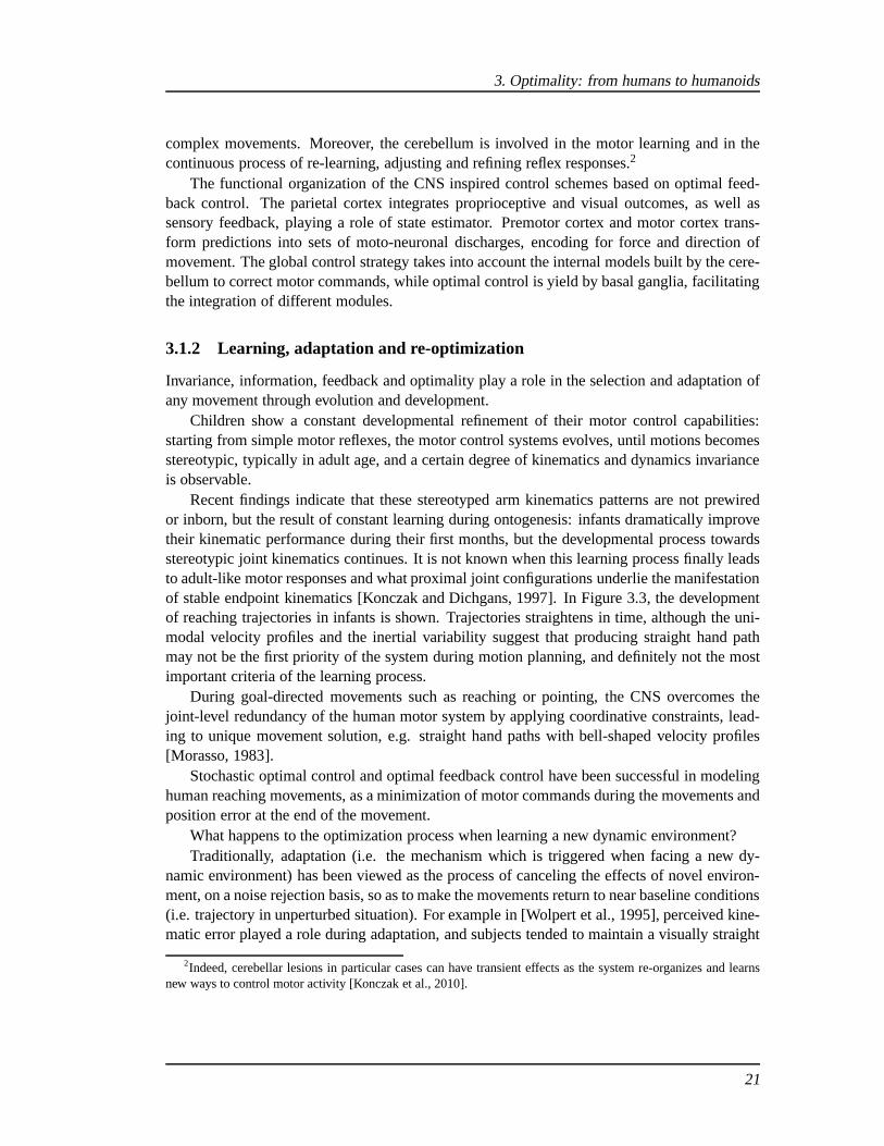
Recent findings indicate that these stereotyped arm kinematics patterns are not prewiredor inborn, but the result of constant learning during ontogenesis: infants dramatically improvetheir kinematic performance during their first months, but the developmental process towardsstereotypic joint kinematics continues. It is not known when this learning process finally leadsto adult-like motor responses and what proximal joint configurations underlie the manifestationof stable endpoint kinematics [Konczak and Dichgans, 1997]. In Figure 3.3, the developmentof reaching trajectories in infants is shown. Trajectoriesstraightens in time, although the uni-modal velocity profiles and the inertial variability suggest that producing straight hand pathmay not be the first priority of the system during motion planning, and definitely not the mostimportant criteria of the learning process.
During goal-directed movements such as reaching or pointing, the CNS overcomes thejoint-level redundancy of the human motor system by applying coordinative constraints, lead-ing to unique movement solution, e.g. straight hand paths with bell-shaped velocity profiles[Morasso, 1983].
Stochastic optimal control and optimal feedback control have been successful in modelinghuman reaching movements, as a minimization of motor commands during the movements andposition error at the end of the movement.
What happens to the optimization process when learning a newdynamic environment?Traditionally, adaptation (i.e. the mechanism which is triggered when facing a new dy-
namic environment) has been viewed as the process of canceling the effects of novel environ-ment, on a noise rejection basis, so as to make the movements return to near baseline conditions(i.e. trajectory in unperturbed situation). For example in[Wolpert et al., 1995], perceived kine-matic error played a role during adaptation, and subjects tended to maintain a visually straight
2Indeed, cerebellar lesions in particular cases can have transient effects as the system re-organizes and learnsnew ways to control motor activity [Konczak et al., 2010].
21

Figure 3.3: Evolution of reaching trajectories in infants. The pictureshows sagittal hand paths ofan infant at different developmental times, showing the progression toward the smoothing of theendpoint motion (image from [Konczak and Dichgans, 1997]).
Figure 3.4: Re-optimization of reaching trajectories when adapting the arm to a new dynamicenvironment. The pictures show a comparison between the baseline trajectory (when the forcefield is null), and the ones learned when the external force field is deterministic (green line, signedσ0) and stochastic (red line, signedσL), with clockwise and counterclockwise orientation (imagefrom [Izawa et al., 2008]).
22

3. Optimality: from humans to humanoids
path in front of perturbations. However, in [Scheidt et al.,2000] it was later shown that kine-matic errors are not necessary for adaptation, i.e. the internal kinematic and dynamic model iscontinuously adapted even in absence of visual kinematic feedback.
In [Mistry et al., 2008] it is shown that humans learn the new force field “dynamically”as opposed to solely rejecting the disturbances via increased stiffness and co-contraction. Indetail, the authors suggested that when facing a novel dynamic environment, the CNS attemptsto return to the baseline trajectory as a methodological strategy to learning an unknown dy-namics. Subsequently, once the internal model is properly learned, the CNS can turn its ef-forts into re-optimizing the motor cost, altering the baseline trajectory if necessary. Similarly,[Izawa et al., 2008] suggested that adaptation entails accuracy and motor cost, and not the kine-matic error from a desired baseline trajectory: thus, a re-optimization process computes a newoptimal motor control trajectory whenever the external force field changes, as shown in Fig-ure 3.4.
Goal-directed movements originate to acquire a rewarding state at a minimum cost, ina stochastic optimal control framework, then it is likely implausible that the brain computes adesired movement trajectory and that trajectory remains invariant with respect to environmentaldynamics. Instead, when the environment changes, the learner performs at least two differentcomputations: update the internal models (i.e. the mappingbetween the consequences of motorcommands in terms of changes in the sensory states) and exploit the refined model to find re-optimize the trajectory planning strategy. As discussed in[Izawa et al., 2008], the cerebellumis the key structure for computing such models, since cerebellar damages produce impairmentsin the ability to adapt reaching to environmental changes. However, the mechanisms for thebrain use this models to re-optimize movements are still uncertain.
In conclusion, motor adaptation entails both learning continuously accurate forward mod-els, compensating environmental changes, and finding the optimal controllers that maximizerewards / minimize costs of planned movements. When facing unpredictable tasks, like pick-ing a box without knowing its load, the CNS initially generates highly variable behaviors, buteventually converges to stereotyped patterns of adaptive responses, which can be explained bysimple optimality principles [Braun et al., 2009].
3.1.3 Feedback and feedforward
Many theories of motor function are based on the concept of “optimality”: they quantify taskgoals as cost functions, and apply the tools from optimal control theory to obtain detailedbehavioral predictions, or to explain empirical phenomena. In the need of anticipating or re-sponding optimally to trajectory perturbations, humans must combine feedback and feedfor-ward signals.
Fast and coordinated limb movements cannot be executed under pure feedback control,because biological feedback loops are too slow (i.e. the delay in the sensory feedback cannotbe neglected - it is about 60ms) and have small gains. Hence, coherently with recent theoriesin neuroscience [Diedrichsen et al., 2010], we believe thatthe CNS solves this and many otherproblems by combining multiple identification and control processes: precisely, exploitingintegrated state estimators, internal models, and feedforward and feedback commands.
The most remarkable property of human movements is that theycan accomplish complex
23

Figure 3.5: The cerebellar feedback error learning model. The “controlled object” block standsfor a physical model of the limbs and body parts controlled bythe CNS. The inverse model is aneural representation of the mapping between desired movement trajectory and corresponding mo-tor commands required to attain the goal, thus it provides a feedforward command. The feedbackcommand can be a simple PID or a more complex controller (image from [Wolpert et al., 1998]).
24

3. Optimality: from humans to humanoids
Figure 3.6: Reaching around an obstacle affects the subsequent trial when there is no obstacle. Leftcolumn shows the trajectories from the control group, reaching with or without an obstacle. Themiddle and right columns show data for a group where two consecutive movements were randomlywith (+) or without (-) an obstacle (image from [Diedrichsenet al., 2010]).
high-level tasks in presence of disturbances, noise, delays, and unpredictable changes in theenvironment. Internal models support such plastic behavior, providing a fast prediction ofthe current system state to the motor controller (anticipating the feedback signals, which forstructural and physical properties come with a certain delay both in humans and robots). Buteven with a quasi-perfect model of the body, open-loop approaches can only yield suboptimalperformances in unstructured stochastic environments. Feedback is then necessary to explainthe performance achieved by the system when adapting its strategies to tasks, environments,physical constraints, since it allows solving a control problem repeatedly rather than repeatingits solution, thus affording remarkable efficiency and plasticity. Figure 3.6 reports the evidenceof the continuous optimization process, which takes into account changes in the environment:when an obstacle impairs unconstrained reaching movements, the normally straight trajectoryis modified to avoid the obstacle. If the obstacle is removed,the CNS does not “switch” tothe control law found without obstacles, but rather adapt the previously found law to the newoptimal one.
Another interesting feature of optimal feedback controllers is that desired trajectories do notneed to be planned explicitly but simply fallout from the feedback control laws. This explainsthe trial-to-trial variability of trajectories performedby humans during repetitive tasks, likehand motion when subjects perform a goal-directed tasks: this variability cannot be explainedby an optimal controller which purely executes trajectory tracking (i.e. if it tracks a pre-defineddesired trajectory), but is captured by an optimal feedbackcontroller that each time tries tominimize global task errors [Scott, 2004].
25

3.1.4 Internal models
Motor control must necessarily incorporate a constant adaption mechanism in order to copewith a changing environment [Shadmehr et al., 2010b]. Sensory feedback is noisy and de-layed, which can make movements unstable or inaccurate, thus it is plausible that, togetherwith feedback control relying on sensory measures, feedforward commands are employed topre-compensate and internal models are used to predict the effect of actions on a changingbody and its surrounding. Such models are usually called “forward models”, as they buildprediction of sensory consequences based on motor commands: as shown in Figure 3.6, theyreceive a copy of the motor commands, called “efferent copy”, eventually access to the cur-rent state of system (even if a connection is not explicitly drawn) and produce a predictionof the sensory consequences of the action, which can be used “immediately” to refine controlstrategies, that is largely before the measured sensory feedback which is inevitably affectedby delays. Predictions from internal models can be used to both calibrate continuously move-ments, and to improve the ability of the sensory system to estimate the state of the body andthe environment. In particular, internal models have a learning dynamics such that predictionof the consequences of adopted controls is learned before they learn to control their actionsin response to task or environmental changes [Flanagan et al., 2003]. Forward models remaincalibrated through motor adaptation: that is, learning is driven by sensory prediction errors.
It is not yet perfectly clear whether the cerebellum contains an explicit representation ofboth forward and inverse models. While forward models seem necessary to compensate for thebiological delays in the sensory apparatus, it is not equally evident if an inverse model (i.e. amodel providing the neural commands necessary to achieve a desired trajectory) exists for allbody parts and corresponding movements.
3.1.5 Optimality and movement duration
Optimal control theory has been recently proposed to explain the mechanisms for movementduration [Shadmehr et al., 2010a]. Human movements show several prominent features, theprincipal being described by [Viviani and Flash, 1995]:
• isochrony principle: movement duration is nearly independent of movement size• two-thirds power law: instantaneous speed depends on movement curvature• movement compositionality: complex movements are composed of simpler elements
Isochrony is strongly connected to the decomposition of complex movements into units of mo-tor action. In [Viviani, 1986] it was suggested that the portion of trajectories with constantvelocity gain factor may correspond to autonomous “chunks”of motion planning, i.e. elemen-tary pieces of trajectories. The isochrony principle applies both globally to the entire trajectory(from the initial to the endpoint) and locally to the small motor actions units. An adequatetheory capable of successfully accounting for all these principles, and explaining motor controlfeatures by means of motor primitives, is still under debate.
In particular, the mechanism underlying the selection of movement duration in the brainis still under investigation. During reaching, curvature path and angular velocity are closely
26

3. Optimality: from humans to humanoids
related, by the so called “two-thirds power law”:
V =KC2/3 =K( 1R)2/3 (3.1)
whereV is the angular velocity,K a velocity gain factor,C the curvature andR the radiusof curvature. This model, proposed by [Lacquaniti et al., 1983], was later extended and re-fined by [Viviani and Stucchi, 1992], and led to many further investigations on its relationshipwith the motion segmentation [Richardson and Flash, 2002] theory, based on the movementcompositionality principle.
The average velocity of point-to-point movements increases with the amplitude of motion,while its duration is weakly dependent on the motion extent.It has been shown that the averagevelocity increase is due both by the velocity gain (depending on the amplitude of motion) andby the distribution of curvatures along the trajectory. These two factors contribute to the relativeinvariance of movement duration, and particularly the strong dependence of velocity gain to theamplitude of motion suggested thatisochronycould best describe this experimental cue.
Most studies in movement duration are grounded on Fitts and Schmidt’ laws [Fitts, 1954,Schmidt et al., 1979], which relates the average movement duration with the amplitude of mo-tion and the error tolerance when reaching the target, on thebasis of either a logarithmic or alinear relationship of their ratio. According to Fitts’ psychomotor model, the time required toaccomplish a movementT is a logarithmic function of the following type:
T = a + b log2 (DW+ c) (3.2)
wherea, b, c are empirical constants [Beamish et al., 2006],D is the amplitude of movement(i.e., the distance between the initial and the endpoint position), andW is the target ampli-tude. ParameterD represents the Euclidean distance between the initial and target points in theCartesian 3D space. The idea is that a certain amount of time is required to perform a move-ment, but the more the movement has to be precise (i.e. we wantto touch a pin instead of a bigball) the more time is required to “adjust” the final positionto the desired. Several analysis andextensions to this law have been done [MacKenzie, 1992], in particular for 2D tasks. Theseand other models, such as the minimum time principle [Tanakaet al., 2006], predict movementduration correctly, but only for point-to-point movements.
More recently, in [Bennequin et al., 2009], a theory of movement timing was proposed, andit was suggested that movement time is continuously selected by the brain based on the combi-nation of different geometrical measures along curves. This hypothesis does not contravene thedescription of the whole trajectory by optimization criteria: on the contrary, invariance is com-patible with different optimization principles such as theminimum-jerk [Flash and Hogan, 1985]or the minimum variance principles [Harris and Wolpert, 1998], and with optimal feedbackcontrol [Todorov and Jordan, 2002], and in general can be used together with optimizationprinciples to solve redundancy problems at the task level, or to control the optimal selection ofthe relevant parameters which could enhance a trajectory description.
27

Figure 3.7: Schematics of the CNS controller proposed in [Kuo, 2005]. Right: A general feed-back control model produces motor commands driving the bodydynamics; sensory processing isused to compute the estimate of the body state. Left: detail of the state estimation, exploiting aninternal model of the body and sensor dynamics, and the efference copy (i.e. the copy of the motorcommand). The integration of multiple sensors is computed optimally, in the sense that feedbackgains are iteratively adjusted to minimize prediction error (image from [Kuo, 2005]).
3.1.6 Optimality and locomotion
Many researchers support the theory that optimization principles also explain the generation ofgait and locomotors trajectories [Mombaur et al., 2008, Arechavaleta et al., 2008]. In humansthe control of posture and goal oriented movement during locomotion is possible through anumber of neural mechanisms, whose controls range to the head stabilization (creating a mo-bile reference frame) [Pozzo et al., 1990], to the exploitation of the vestibular system, to thegeneration of trajectories. Again, different models have been proposed.
In [Kuo, 2005] an optimal model for estimation and control ofhuman postural balance isproposed. Assuming that the CNS estimates the postural “state” with a certain delay, and thatthis estimate is used to produce a feedback control to stabilize the system, as shown in Fig-ure 3.7, the author propose a computation model based on stochastic optimal control. In detail,a linear quadratic controller is addressed, where the cost function is the sum of quadratic termsweighting the joints displacement from the equilibrium configuration and the neural effort, i.e.the amount of muscle activation used to stabilize the system; sensory noise is taken into accountin the model, both as body model and transducer noise. Similarly, in [Lockhart and Ting, 2007]it is argued that an optimal control model with delayed feedback rule is at the basis of the neu-ral effort produced by mammalians to keep the balance. Particularly, a feedback control law (acombination of the errors of position, velocity and acceleration of the COM of the body withrespect the stable steady configuration) was optimized according to a quadratic cost function,weighting COM kinematic deviations and muscle effort (fromEMG measurements).
3.2 Which is the correct “cost function”?
Stochastic optimal control theory provides an elegant mathematical framework for describingmovements: by the notion of “motion criteria” transposed into “cost function” or “reward func-
28
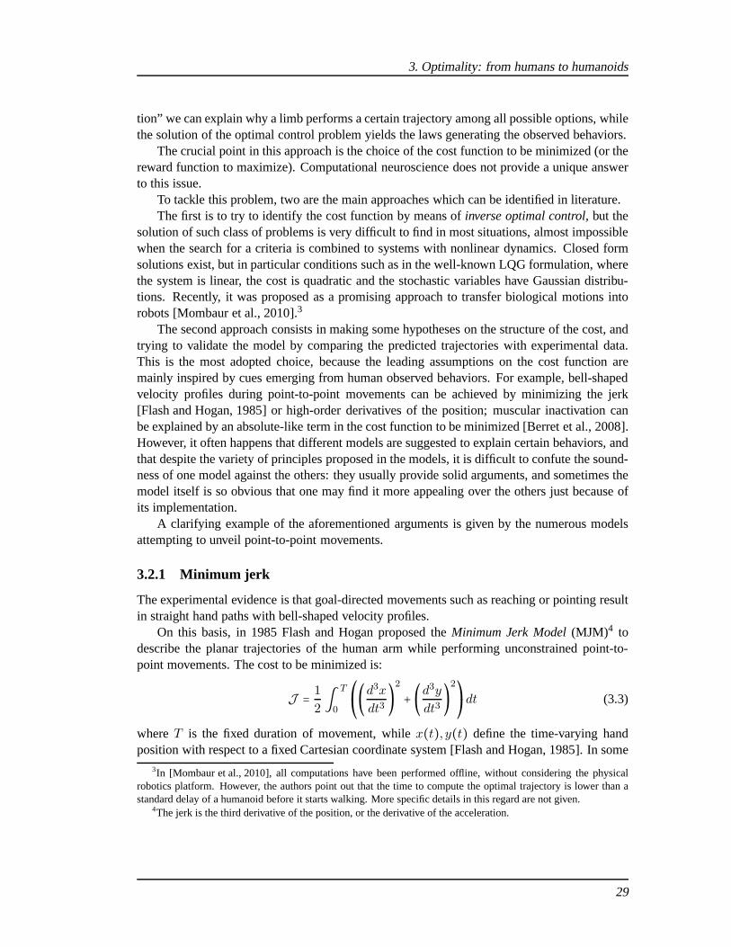
3. Optimality: from humans to humanoids
tion” we can explain why a limb performs a certain trajectoryamong all possible options, whilethe solution of the optimal control problem yields the laws generating the observed behaviors.
The crucial point in this approach is the choice of the cost function to be minimized (or thereward function to maximize). Computational neurosciencedoes not provide a unique answerto this issue.
To tackle this problem, two are the main approaches which canbe identified in literature.The first is to try to identify the cost function by means ofinverse optimal control, but the
solution of such class of problems is very difficult to find in most situations, almost impossiblewhen the search for a criteria is combined to systems with nonlinear dynamics. Closed formsolutions exist, but in particular conditions such as in thewell-known LQG formulation, wherethe system is linear, the cost is quadratic and the stochastic variables have Gaussian distribu-tions. Recently, it was proposed as a promising approach to transfer biological motions intorobots [Mombaur et al., 2010].3
The second approach consists in making some hypotheses on the structure of the cost, andtrying to validate the model by comparing the predicted trajectories with experimental data.This is the most adopted choice, because the leading assumptions on the cost function aremainly inspired by cues emerging from human observed behaviors. For example, bell-shapedvelocity profiles during point-to-point movements can be achieved by minimizing the jerk[Flash and Hogan, 1985] or high-order derivatives of the position; muscular inactivation canbe explained by an absolute-like term in the cost function tobe minimized [Berret et al., 2008].However, it often happens that different models are suggested to explain certain behaviors, andthat despite the variety of principles proposed in the models, it is difficult to confute the sound-ness of one model against the others: they usually provide solid arguments, and sometimes themodel itself is so obvious that one may find it more appealing over the others just because ofits implementation.
A clarifying example of the aforementioned arguments is given by the numerous modelsattempting to unveil point-to-point movements.
3.2.1 Minimum jerk
The experimental evidence is that goal-directed movementssuch as reaching or pointing resultin straight hand paths with bell-shaped velocity profiles.
On this basis, in 1985 Flash and Hogan proposed theMinimum Jerk Model(MJM)4 todescribe the planar trajectories of the human arm while performing unconstrained point-to-point movements. The cost to be minimized is:
J = 1
2∫ T
0
⎛⎝(
d3x
dt3)2 + (d3y
dt3)2⎞⎠dt (3.3)
whereT is the fixed duration of movement, whilex(t), y(t) define the time-varying handposition with respect to a fixed Cartesian coordinate system[Flash and Hogan, 1985]. In some
3In [Mombaur et al., 2010], all computations have been performed offline, without considering the physicalrobotics platform. However, the authors point out that the time to compute the optimal trajectory is lower than astandard delay of a humanoid before it starts walking. More specific details in this regard are not given.
4The jerk is the third derivative of the position, or the derivative of the acceleration.
29

peculiar conditions, closed-form solutions forx(t), y(t) can be found. For example, given theboundary conditionsx(0) = x0, y(0) = y0, with zero velocity and acceleration at the beginningand end of the trajectory,x(0) = y(0) = x(0) = y(0) = 0, x(T ) = y(T ) = x(T ) = y(T ) = 0,the explicit solution is:
x(t) = x0 + (x0 − xf)(15τ4 − 6τ5 − 10τ3)y(t) = y0 + (y0 − yf)(15τ4 − 6τ5 − 10τ3) (3.4)
whereτ = t/T ∈ [0,1]. Extensions to non-null boundary velocities, path segmentation throughmultiple “via points” easily follow.
It must be noted that trajectories are purely kinematics andare completely independentof the dynamics of the arm. However, the trajectories predicted by the MJM are straight-lineCartesian paths with bell-shaped velocity profiles, which is consistent with the experimentaldata for rapid human movements in absence of accuracy constraints.
The MJM is defined in an extrinsic-kinematic space (i.e. Cartesian space). An analogousmodel, defined in the arm joint space, was proposed in 1995 by Rosenbaum et al., where thefunction
J = 1
2∫ T
0
n∑i=1
(d3θidt3)2 dt (3.5)
whereθi is thei-th joint angle. The model was called Minimum Angle Jerk Model (MAJM),always predicted straight paths in the joint space but in contrast to the MJM it allowed torepresent trajectory curvatures.
3.2.2 Minimum torque change
The main defect of the MJM is that it always predict straight paths, so it does not fit to widerange movements and curved trajectories which occur for example during transverse move-ments, regardless of the influence of arm dynamics, arm posture, external forces, and move-ment duration.
Overcoming this issue, in 1989 Uno et al. proposed theMinimum Torque Change Model(MTCM), where trajectories were selected so as to minimize the rate of changes in torques,precisely:
J = 1
2∫ T
0
n∑i=1
(dτidt)2 dt (3.6)
whereτi is the torque at thei-th joint of the chain [Uno et al., 1989]. The MTCM takes intoaccount the arm dynamics, and is able to reproduce graduallycurved trajectories. One con-troversial point in the MTCM is whether the CNS actually minimize torques, which seem tobe difficult to estimate and integrate over a real trajectory(being dependent on the musclesdynamics). Computing an optimal trajectory with the MTCM isactually demanding.
Ten years later, Nakano et al. proposed a variant of MTCM, called TheMinimum Com-manded Torque Change Model(MCTCM) [Nakano et al., 1999], which provided a computable
30

3. Optimality: from humans to humanoids
Figure 3.8: A schematic representation of the main difference between MTCM and MCTCM(image from [Nakano et al., 1999]).
approximation of the MTCM while taking into account both link and muscle dynamics.5 Aschematic representation of the two models is shown in Figure 3.8. The cost to be minimized isidentical in both MTCM and MCTCM: the main difference between the two is the dynamicalmodel of arm and muscles used to compute the torque commands.The MCTCM confirmedexperimental observation in humans (see Figure 3.9), whereother models such as MJM failedto reproduce trajectory curvatures depending on movement location and direction representedin intrinsic body coordinates. Their results indicated that CNS may plan optimally in intrinsiccoordinates considering the arm muscles dynamics and usingmotor commands representationswhich include muscle tension.
3.2.3 Minimum variance
In 1998 Harris and Wolpert observed that both eyes and arm movements were generated byneural controls corrupted by a signal-dependent noise, i.e. whose variance was proportional tothe amount of control signal itself. Thus, rapid motions, requiring larger control signals, woulddeviate from the desired trajectory as an effect of the disturbed control, resulting at the end inunsuccessful or imprecise final positions [Harris and Wolpert, 1998]. Thus, they proposed theMinimum Variance Theory(MVT) which states that the accuracy in goal-directed movementsis maximized by minimizing the variance of the final configuration. The MVT speed-accuracytradeoff agrees with Fitts’ law; moreover explains why repeated movements generally improvelimb motion, as optimal trajectories can be learned during exercise.
3.2.4 The Inactivation Principle
In 2008 Berret et al. proposed a cost including a term called “absolute work of forces”, re-flecting the mechanical energy effort of a motion. In contrast to previous models, this term isnon-smooth and non-differentiable, being based on an absolute function, however it is reason-able since it is grounded on the Inactivation Principle [Berret et al., 2008]. According to this
5The MTCM assumes null viscosity in the arm model, while MCTCMuses a non-null viscosity matrix incalculating the joints torques, thus considering both linkdynamics and muscles as controlled object in the model.For more detail, see [Nakano et al., 1999].
31

(a)
(b)
Figure 3.9: A comparison among different motor control models.3.9(a)Observed and predictedplanar trajectories.3.9(b)observed and predicted velocity, acceleration and torque profiles duringplanar trajectories (images from [Nakano et al., 1999]).
32

3. Optimality: from humans to humanoids
Figure 3.10: Velocity profiles of a pointing finger, and EMG recordings of the muscles during 1DOF arm upward and downward movements. The speed profiles show muscular inactivations inproximity of velocity peaks (DA/DP=Deltoid Anterior/Posterior, BI=Biceps, TR=Triceps - imagefrom [Berret et al., 2008]).
principle, supported by experimental observations from EMG signals (see Figure 3.10), mini-mizing absolute terms implies simultaneous inactivation of agonistic and antagonistic musclesacting on a single joint, near the time of peak velocity. In detail, the proposed cost is of thefollowing type:
J = ∫ n∑i=1
∣τiθi∣ +αiθ2
i (3.7)
Notably, (3.7) accounts for a hybrid model, where both kinematics and dynamics variables aretaken into account.
3.2.5 Which cost function?
Table 3.1 reports a summary of the aforementioned cost functions, and of many others, and stillit is not fully comprehensive of all the models that have beensuggested in literature. From thepoint of view of an engineer, it is difficult to choose which among the proposed models shouldbe implemented on a robotic manipulator or sustained for future implementations.
One possible criteria to choose a model could be its explicitsolution, for only those mod-els with closed form solution could be implemented easily. This criteria rules out all modelsexcept the MJM, but explains why it is frequent to find comparisons between its predictionsand experimental data from observed behaviors in humans. Overall, this model is quite ap-pealing for roboticists too: since the analytical solutionis provided (and it is also very simple),its implementation is straightforward. Furthermore, jerkminimization is beneficial if control
33

Criterion Cost functionJ References
Hand jerk ∫ T0
...x2 + ...
y 2dt [Flash and Hogan, 1985]
Angle jerk ∫ T0
...θ1
2 + ...θ2
2
dt [Wada et al., 2001]
Angle acceleration ∫ T0
θ12 + θ22dt [Ben-Itzhak and Karniel, 2008]
Torque change ∫ T0
τ12 + τ22dt [Uno et al., 1989]
Torque ∫ T0
τ21 + τ22 dt [Nelson, 1983]Geodesic ∫ T
0[θ⊺M(θ)θ]1/2dt [Biess et al., 2007]
Energy ∫ T0∣θ1τ1∣ + ∣θ2τ2∣dt [Berret et al., 2008]
Effort ∫ T0
µ21 + µ2
2dt [Guigon et al., 2008]
Table 3.1: Different cost functions (and related computational motorcontrol models) for point-to-point movements.
strategies must be implemented on real devices: since the velocity and acceleration profiles arevery smooth, the system is less “stressed”.
From a robotics perspectives, one desirable feature is to produce controls which do notstress the mechanical structure of the manipulator or tend to minimize energy efforts. In thissense, MCTM or MCTC support this motivation, even if the biological counterpart seems a bitunclear.
It must be also pointed out that in humanoids robots motion trajectories can be controlledeither with kinematics or dynamics loops, e.g. with joints velocity or joint torques. Thus,control variables must be taken into account as decision criteria.
The conclusion of this argument is twofold: first, in computational neuroscience there aremany sounds models that can be used to study and describe human motions; second, manymodels are eligible for implementation in robotics, and thechoice is basically application androbot dependent.
As if all this was not enough, recently some researchers debated the structure of this costs[Nagengast et al., 2011]. In particular, they suggested that humans not only optimize the aver-age cost associated to a movement, but being risk-sensitive, while optimizing the mean payoffthey also take into account the variability of the payoff itself. In other words, they minimize theaverage cost together with its mean variance. According to the authors, early experimental re-sults suggested that the CNS acts like a risk-sensitive decision maker, which trades off the meanand the variance of movement effort. These claims suggest that the stochastic optimal controlframework alone may not be sufficient to address the optimization problem behind motor con-trol, and that other mathematical tools like decision theory and multi-objective optimizationshould be inevitably taken into account.
3.3 Optimality: from humans to humanoids
In the previous section an overview of the main features of human motor control was presented.Despite the incredible number of research studies and experiments, we still do not known pre-cisely which are the correct mechanisms underlying the CNS controlling and learning complex
34

3. Optimality: from humans to humanoids
motor skills, except that most models assume optimal feedback control as a framework for mo-tor control. All models are sound and could be advantageous for robotics, but require differentimplementations.
Nowadays, in robotics great attention is devoted to reproduce the behavior and the learn-ing mechanisms of living creatures, developing systems that exhibit and replicate the controland learning abilities observed in animals or human beings.While modern mechatronics hasreached great results (even within technology limitations), and humanoid robots exhibit shapesand structures which closely imitate humans, the great challenge is still to reproduce the learn-ing processes and the interactions between the brain and thesensory and nervous system, thatgenerate controls, emotions etc. and that could provide therobot with a real intelligent control:the challenge is cognitive control [Metta et al., 1999, Sandini et al., 2004].
Computational motor control models can provide useful guidance in the design of ad-vanced control solutions for robots. Actually the two areasof research benefit from mutualachievements [Schaal and Schweighofer, 2005], because many problems faced by the primatebrain in the control of movement have parallels in robotic motor control, while models andalgorithms from automatic control and robotics research can bring useful inspiration, baselineperformance, and sometimes direct analogs for neuroscience.
Indeed, it is our belief that only with the study of the human it is possible to build bettercontrols for humanoid robots.
As engineers, we aim to a control policyu(t) = γ(x(t),w), whereu is a control vector,γ a control function or policy,x the system state vector andw a set of parameters whichdetermine the policy. A policy can resort into direct control (i.e. direct generation of motorcommands) or indirect control, that is the most common case in robotics, where for exampledesired planned trajectories are converted into motor commands (in this case, decoupling thesystem can notably simplify the control architecture).
The policy itself or its parameters (or both) can be fixed or adaptive. In the latter case, ifthe control problem is stated as an optimal control problem,an optimization routine can be setso that policy and parameters can be found, e.g.
γ,w = argminJ (x(t), u(t))s.t. u(t) = γ(x(t),w)
whereJ is the cost function defining the motion criteria.In automatic controls there is a vivid research in the designof optimal control laws and the
solution of such optimization problems, which sometimes can also have explicit solution (e.g.thanks to Riccati’s equations, under the well-known LQG assumptions) [Vidyasagar, 1987,Bertsekas and Tsitsiklis, 1996, Sastry and Bodson, 1994]. Many application of optimal con-trols to robotics refer to classical approaches: for example in [Kim et al., 2000], where a robustcontrol is found combining a stabilizing control (based on Riccati and Lyapunov equations) anda neural network accounting for unknown dynamics; in [Barambones and Etxebarria, 2002] arobust neural sliding mode controller is presented, while tracking controllers are discussed in[Sun et al., 2002, Braganza et al., 2005]. However, the high complexity and the desire to de-sign an adaptive plastic system, as close as possible similar to the human, impose limitationson the use of classical controls, even if they provide a wide and assessed theory for stability,
35

convergence and optimality. The main limitation of such classical control schemes is that theyare not suitable for cognitive functionalities. The biological inspiration we seek, force us toovercome the limits of traditional automatic controls, andchoose new schemes to emulate theadaptation and learning capabilities of humans, combined with the optimality principles whichhave been observed experimentally.
Thus, we need more specific tools. In this perspective, we must design a suitable controlscheme, which can guarantee all the good properties (such asstability, robustness, etc.) thattraditional automatic control have; which can possibly benefit from decoupling and simplifyingthe systems and the control architecture, exploiting modularity; which is naturally arranged tobe integrated with one or multiple learning mechanisms. Moreover, we need a mathematicaltool which is able to compute trajectories and controls “optimally”: it must be able to solvea general optimal control problem given the problem statement, the computational model andthe cost function to be minimized.
In the following, we will briefly present the state of the art implementations of biologicallyinspired optimal control in robotics, particularly in humanoid robotics. Finally, we will intro-duce the key aspects of our proposed framework, to motivate the mathematical tool describedin this work. Some insights of future developments will be also given.
3.3.1 Some implementations of optimal control models in robots
Reaching
Among the computational models presented in Section 3.2, only few have been actually imple-mented on real robotic platforms. An analytical solution exists (and can be easily implemented)for the MJM and the MAJM. An interesting implementation of a MJM based controller forthe iCub robot can be found in [Pattacini et al., 2010]. An implementation of the MVT fora 2DOF arm was done in [Simmons and Demiris, 2005]. Models involving torques, such asthe MCTCM, require the arm dynamics, thus a constrained nonlinear optimization problemmust be solved, minimizing the cost function under some constraints (the nonlinear dynamics)and the boundary conditions (start and final configuration ofthe arm, physical limits). Thesolution of this class of problems is generally difficult, and depending on the problem state-ment there could be more than one method (or none) suited for its solution. For example, in[Kaneko et al., 2005] a solution to the MCTCM is found by meansof a numerical optimizationof the Euler-Poisson equation: though describing a generalprocedure, the authors admit theimpossibility to guarantee the convergence of the routine,thus making the algorithm unsuit-able for real-time planning or control in robotic applications. In [Shiller and Dubowsky, 1991]optimal control is used to compute time-optimal motions of arobotic manipulator, consideringnonlinear dynamics, actuator constraints, joint limits, and obstacles. In [Zhao and Chen, 1996]an optimal motion planning is addressed to control a flexiblespace robot, in order to minimizethe maneuvering time along with control and vibration energy. In [Mettin et al., 2010] an op-timal control problem is used to find controls for ball pitching with an under-actuated 2DOFhuman-like arm, where in particular only the shoulder is actuated while the elbow is a pas-sive spring with adaptive stiffness: the criteria is to maximize the ball velocity along a certainelevation angle. In [Matsui, 2008, Matsui et al., 2009] the authors propose an experimentally-
36

3. Optimality: from humans to humanoids
validated 3DOF model of the human arm during constrained andunconstrained reaching move-ments, where the criterion (i.e. the cost to be minimized) isbased on energy and torque change,constrained by the hand-joint’s freezing mechanism, explaining the experimental fact that thehand joint hardly changes its angle during reaching movements. Again optimal control theoryis used to find the optimal trajectories of the hand during goal-directed motions.
Locomotion
The use of optimal control for humanoids has become recentlypopular to solve the gait andlocomotion problems, and particularly both for stabilizing the robot and to plan optimally walk-ing trajectories [Chevallereau and Aoustin, 2001, Kanoun et al., 2009]. In [Tlalolini et al., 2011]the authors suggest that human walking analysis could improve the current humanoid robotswalks, an particularly to reduce the energy consumed duringwalking. In detail, they prove thata foot rotation subphase (specific during human fast walking) introduced in the gait contributesto the minimization of a torques-based cost, thus yielding optimal motions.
In [Arechavaleta et al., 2008] the authors investigate human goal-directed walking, with theunderlying assumption that locomotors trajectories are chosen according to some optimiza-tion principle. With the attempt to identify the criteria which are optimized (duration, length,etc.), they found that the time derivative of the curvature is minimized, and that trajecto-ries are well-approximated by the geodesics minimizing theL2 norm of the control, shapedas clothoids6. In [Whitman and Atkeson, 2009] dynamic programming is usedto optimizebody motion, foot placement and step timing for a two link inverted pendulum model. In[Schultz and Mombaur, 2010] running is modeled as a multiphase periodic motion with dis-continuities, based on multibody system models of the locomotors system with actuators andspring-damper elements at each joint; thus, running motions are generated as the solution ofa an optimal control problem, based on energy criteria, solved by an efficient direct multipleshooting algorithm. In [Blair and Iwasaki, 2011] the authors suggest that the basic principleunderlying animal locomotion is a mechanical rectificationthat converts periodic body move-ments to thrust force through interactions with the environment: thus, an optimal gait problemis formulated, where a quadratic cost function is minimizedover a set of periodic functionssubject to a velocity constraint, and the system is represented by a bilinear dynamic model,assuming small oscillations with respect to a nominal posture. In [He and Geng, 2007] optimalcontrol is used for stable jumping of a one-legged hopping robot, with the goal to maximizeenergy efficiency of the motion. In [Lengagne et al., 2009] optimality is again exploited tomake kicking motions more accurate, exploiting a combination of an off-line planning aimedbasically at minimizing torques, with a fast re-planning process, which adapts the controls de-pending on the current target configuration. In detail, the cost function they try to minimizein the planning step is the sum of squared joints torques, which corresponds to the goal ofimproving the robot autonomy. As an optimization tool, the authors use IPOPT. The authorspoint out the limitations of their method, by admitting thatthe optimization of an instance ofthe problem takes about two hours CPU time (without more specific details).
6The clothoid or Cornu spiral is a curve, whose curvature grows with the distance from the origin.
37

3.3.2 Computational limits
Implementations of the aforementioned biologically inspired models on humanoid platformsface notable computational limits, since most optimal control problems incur into the COD, andeven the solution of simplified problems (e.g. after strong hypotheses cutting the complexityof the model) cannot always guarantee the fulfillment of timeconstraints [Diehl et al., 2009].Rather than searching for a generalized solution to the planning problem, whose computationallimits make it unsuitable for online real-time control, many proposed approaches in literatureusually focus on the optimization of single point-to-pointmovements [Simmons and Demiris, 2005,Matsui et al., 2006, Seki and Tadakuma, 2004, Tuan et al., 2008].
The corresponding optimal control problems are usually tackled via numerical methods andnonlinear programming algorithms, but the optimization process requires heavy computationsand often prevents the application in real-time.
As an example, in [Tuan et al., 2008] a single movement generation is reported to takefrom 1 to 4 minutes, even with a fast optimizer as IPOPT [Wachter and Biegler, 2006]. In[Bauml et al., 2010], the optimization of a single trajectory for a 7DOF arm is performed inreal-time, but under numerous assumptions regarding the system dynamics and kinematics, andmost of all by a parallel computation on a cluster of 32 CPU cores, yielding 80% of success inthe desired task.
Since closed-form solutions are utterly hard to find (impossible in many cases) approximatesolutions can be addressed.
For example, Nonlinear Model Predictive Control (NMPC) methods can be used, but eventhe explicit precomputation of NMPC laws is prohibitive forstate/parameters aboveR10. Forexample, in [Diehl et al., 2006] a NMPC with fast direct multiple shooting algorithm and sev-eral approximations were made to reduce a 20 CPU seconds computations on a 3GHz PentiumIV to 200ms, for a 5 state150ms trajectory. The reader should see [Diehl et al., 2009], whereoff-line precomputation, delay compensation and other techniques were surveyed, discussingreasonable compromises between computational time, convergence of the method, approxima-tion performances and real-time guarantee.
One remarkable point is that optimal control schemes applied in robotics must take intoaccount the platform constraints, and particularly the hardware and software limitations. Forexample, the generation of direct joint-level control mustcomply with their control loop rate(e.g. 1KHz in iCub and James); simultaneously, it requires aconsiderable amount of computa-tions, both in term of time and resources. Thus, despite local computations should be preferredbecause they could fasten the control cycle, it may not be feasible to perform such processingon local boards (i.e. the boards directly connected to the joints) if they have limited processingcapabilities. This, which is the case of iCub and James, implies that most computations mustbe performed by one or more PC in a cluster, which is remotely connected to the robot; in thisconfiguration, real-time constraints cannot be a priori guaranteed, and in general the safety ofthis controls can be solved only up to a certain level.
38

3. Optimality: from humans to humanoids
3.3.3 A layered control scheme
The implementation of cognitive control for a complex humanoid robot is a challenge. An intel-ligent control system, modeled after biological systems and human cognitive capabilities, mustpossess learning, adaptation and classification capabilities, providing improved performanceswith respect to classical controls, but guaranteeing stability and adaptation in the presenceof unknown disturbances, unmodeled dynamics (because the modeling is too difficult or be-cause these dynamics have been neglected), and unstructured uncertainties [Metta et al., 1999,Sandini et al., 2004].
The control architecture we propose is particularly targeted for those systems where somecomputations can be only performed remotely. In detail, we support a layered architecture,where the task planning level is decoupled from the generation of low-level commands. Thetransformation between the two spaces can be performed by anintermediate level, which isbasically constituted by an Inverse Kinematics (IK) moduleand eventually by a Forward Dy-namics (FD) module, as shown in Figure 3.11.
Remark 1. The layered architecture proposed hereinafter, reflects a traditional pattern ofreaching, considered a two-stage process, where a planningphase is followed by an executionphase (and planner and controller can be two separate modules). This traditional view hasbeen challenged by the dynamical system approach to movement control, claiming that thereis no explicit trajectory planning, but rather an implicit set of trajectories which are generatedby a dedicated dynamical system. An example is the VITE model[Hersch and Billard, 2006].Here, we do not support such schemes, even if our technique iscapable of coping with thedynamical systems theory.
PlanningTask
OptimalROBOTTask to Joint Space
J x∗, x∗ τ∗ or q∗
Figure 3.11: A conceptual scheme of a classic hierarchical control scheme for robotics. Thetask parameters, such as the control function to be minimized, the current status of the robot, thetask goal etc. are fed to the optimal planner, which computesthe optimal trajectory, typically inthe operational space (e.g. Cartesian space). An intermediate layer is in charge with convertingcommands from operational to joint space. In this scheme, feedback loops are not voluntarilydepicted.
The planning module is the core of this work. To describe the planning problem as anoptimal control, the modeler has to specify:
• a family of admissible control laws• a quantitative definition of task performance• a compatible robot kinematics and dynamics model
The latter is usually known, since the kinematics and dynamics model of the robot is in generaleasy to find from the CAD specifications, thus the robot can be described by means of a set of
39

differential equations. In general, parameters are not perfectly known, and many dynamics can-not be fully modeled, so a supervised learning model could beused instead. The task is insteadspecified by a cost function: this usually comes with the computational motor control modeladopted to plan the movement. The family of admissible control laws is difficult to choose,a priori, because it is strongly connected both to the robot model and to the task. Planningoptimally a trajectory according to some principles, in a stochastic optimal control framework,is generally a tough problem. Without a priori hypotheses onthe structure of the problem (cost,system model, constraints, etc.) it is impossible to state whether a given algorithm is guaran-teed to yield a solution within a certain time. In Chapter 4 wewill present a method to computeoptimal trajectories, which concentrates the computationin an offline phase, but under suita-ble assumptions allow retrieving almost instantly the solution online, taking into account thefeedback on the current status of the system. Moreover, given the particular structure of ourcontroller, we will show that not only it is possible to learnthe optimal solution online thoroughan intensive learning phase, but it is possible to update thesolution incrementally, combiningcontrol and adaptation, in case for example the system changes.
The IK and FD can be both learned from experimental data, or estimated if an accuratemodel of the robot kinematics and dynamics is available. In Chapter 5 we will discuss somepossible methods that can be used, along with their advantages and disadvantages.
3.3.4 Orchestration in a control scheme: team theory
The optimal controllers inspired by the CNS and the many motor control models must be ob-viously integrated in the robot Cognitive Architecture (CA), that is the software system thatimplements the processes of the CNS [Vernon et al., 2007b] and constitute the effective “intel-ligence” of the robot. The CA usually consists of a set of independent modules, interconnectedaccording to hierarchy, antagonism and cooperation, including all the relevant aspects for themodules across different application domains7.
The primary requirement of a CA is to provide a complete perceptual representation of therobot state: the robot is a complex plant, subject to a continuous excitation of its sensory sys-tem, including all types of sensors, from proprioceptive (e.g. encoders) to visual (e.g. cameras)and tactile (e.g. skin).
There are many technological challenges in dealing with a great amount of sensor-collecteddata [Albers, 2002], in generating new actions and control strategies, and in the meantimein learning through data and interaction with environment,in self-organizing and adaptingsensor strategies. Our belief is that motor control models,represented as stochastic optimalcontrollers, could be integrated and enriched in significance in the context of a team theoryframework.
Team theory is an area of game theory (see [Radner, 1962, Ho and Chu, 1972]) that pro-vides a mathematical framework which can easily describe the cooperation among devices,such as sensors and controllers, hereafter named asDecision Makers(DM), in highly complexsystems. A team is a family of autonomous devices able to perform a task. It can often been
7Decision making, at any level; attentive system; prediction and internal models of self and environment; rea-soning; autonomous exploration; memory and learning, etc.
40

3. Optimality: from humans to humanoids
viewed as a network in which each team member controls, observes, measures, gets differentinformation, and decides to elaborate, share or transmit some personal information to the otherteam members, trying to maximize some common benefit or minimize a common cost.
The CNS can be modeled by a dynamic systemS, resulting from the aggregation ofNdynamic subsystemsS1, S2, . . . , SN , connected among them, interacting, and evolving in asynchronous way. We conjecture that human “controllers”, either performing high-level ac-tivities (e.g. learning, memory) or generating simple loops, can be represented as a familyof different DM, each having a different task, processing capabilities and reacting to differentstimuli. Each decision makerDMi acts on one or more subsystems, as a controller or, whenbehaving as intelligent sensor, it generates the signals tobe sent to the other decision makers.In all cases,DMi influences the decisions and the behavior of the other team decision makers.
Whenever a dynamic system is controlled by a plurality of decision makers, a first probleminsists in identifying the goals pursued by the decision makers. Within the human organism,it is reasonable to presume that controllers, sensors, and organs, though having different infor-mation, cooperate to the accomplishment of a common goal: wellbeing, growth (learning) andhealth of the living being. The existence of cooperation among the decision makers and thefact they possess “individual” information lead us to statethe problem of their cooperation inthe framework of team theory.
More specifically, ifN decision makersDMi, i = 1, . . . ,N , cooperate to the minimizationof a common cost functionalJ , the optimization problem can be stated as follows:
minγ1,...,γN
E J [γ1(I1), . . . , γN(IN), ξ] ,whereξ represents a set of exogenous random variables,γi is DMi’s decision or control func-tions, andIi is its information vector. The expectation is evaluated with respect toξ.
The solution of a team optimal control problem is a hard task,and can be solved, in ge-neral, only through approximation methods. However, thereare many examples in literatureof solutions exploiting functional approximators [Zoppoli et al., 2011, Baglietto et al., 2001b,Zoppoli et al., 2002, Baglietto et al., 2001a]. Even in this case these methods allow obtainingapproximate solutions to such functional optimization problems, that benefit by the fundamen-tal property of not incurring the COD phenomenon,” i.e., theexponential growth of the numberof parameters with the complexity (suitably measured) of the problem dealt with.
In this perspective, using ANN to approximate the optimal planning control functionsseems a promising approach, which could be integrated in a more complex scenario wheremultiple controllers or more generally decision makers, cooperate for the achieving of a com-mon goal.
41

42

Chapter 4
Optimal control by means offunctional approximators
4.1 Planning “optimally” goal-directed movements
In robotics, the task of positioning the end effectors and toreach a goal is fundamental: when-ever a robot has to move its arm to grasp an object, track a moving target, avoid collision withthe environment or just explore, reaching is involved [Brock et al., 2008, Nori et al., 2007b].Given the desired position it is common practice to plan a suitable trajectory in the Cartesianspace using parameterized functions (e.g. polynomials or splines) and then to find the cor-responding joint or torque commands analytically, exploiting traditional robotics schemes toperform the conversion from the operational space into joint space.
In humanoid robotics, the focus is not only on reaching the target, but on the way the targetis reached, that is the criterion which the limbs accomplishwhile performing a movement. Oneof the main goals of humanoid robotics is indeed to exploit redundancy and constraints of thehumanoid shape to achieve behaviors that are approximatelyas efficient as human movements,and to provide a testing platform for computational models,such as the ones presented inChapter 3. In this perspective, a technique must be providedto the robot which allows findingoptimal control commands for any given cost function or task, implementing different motioncriteria.
Design of optimal control laws for robots is not new. In the area of automatic controls,there’s a tradition in using simple and robust controls which yield to optimal control laws (i.e.solving a LQ problem by Riccati’s equations). However, the biological inspiration force us toovercome the limits of traditional automatic controls, which are not sufficient to implement theadaptability of the control laws to new tasks, criteria and unknown dynamics.
The goal of the planning module is to find the optimal trajectory which makes the end-effector accomplish a certain task in an optimal fashion, i.e. minimizing a given cost func-tional. It must be quick, i.e. not computationally demanding in terms of time and resources,reactive to unpredictable target’s changes, able to cope with the manipulator’s physical limita-tions (singularities, joint limits, etc.) and control architecture.
A planning policy can resort into direct control or indirectcontrol:
43

• direct control accounts for direct generation of motor commands, joint-level, of the fol-lowing type:
τ∗ = γ(x) or q∗ = γ(x)whereτ, q ∈ Rn are the vector of joint torques and joint velocities, respectively (thusreferring to joint torque or joint velocity control schemes), andx the operational spaceconfiguration of the end-effector
• indirect control, that is the most common case in robotics,where for example desiredplanned trajectories are converted from the operational space into motor commands inthe joint space, for example by means of Inverse Kinematics (IK) or Forward Dynamics(FD) modules:
x∗ = γ(x) then q∗ = IK(x∗, x∗), τ∗ = FD(q∗, q∗)Sometimes it is better to segregate the trajectory planningfrom the trajectory execution, so thatit is possible to tune both modules separately: in this case,indirect control is preferred.
Among different possible approaches, we decided to state the planning problem as a Fi-nite Horizon (FH) or Receding Horizon (RH) problem, and to use functional approximationtechniques in order to approximate numerically the global solution to the optimization prob-lem, to pre-compute the optimal control laws. The RH approach becomes necessary wheneverthe duration of the movements cannot be predicteda priori. One argument is that the dura-tion of motion can be found by computational models like the ones described in Section 3.1.5(e.g. Fitts’ law ). Unfortunately, it is difficult to cast similar predictions for humanoid robotsand to generalize these models for different tasks such as tracking or reaching. Nevertheless,the RH solution comes for free since it is immediately available once the generalized FH so-lution is found, for example by applying at each time instantonly the first FH control law[Parisini and Zoppoli, 1995], as will be explained later on.Having both solutions available,we can tailor the solution depending on the task: e.g. a FH strategy is more suited for purereaching movements, while a RH strategy for tracking targets moving indefinitely.
Trajectory planning finally consists in the computation of atime-invariant, feedback, stochas-tic optimal control law. In detail, a suitable sequence of neural networks is trained off line, sothat they can approximate the optimal solutions of a stochastic FH control problem, whichis generalized for every possible state configuration (i.e.every possible system and targetstates belonging to an opportune set of admissible states).The Extended RItz Method (ERIM)[Zoppoli et al., 2002] is chosen as a functional approximation technique, while the use of feed-forward neural networks (thanks to their well-known approximation capabilities [Barron, 1993])guarantees that the optimal solutions can be approximated at any desired degree of accuracy[Kurkova and Sanguineti, 2005] by using a parsimonious number of parameters to be opti-mized.
In this way, the computation demand is concentrated in the off-line phase, while in theon-line phase only the computation of a single control law (corresponding to a neural networkforward) is performed et each time. Thus the control action is generated with a very smallcomputational effort. The feasibility of this approach hasalready been tested on the controlof a thrusts-actuated nonholonomic robot [Ivaldi et al., 2008c]. Numerical results showing itseffectiveness for different cost functions were presentedin [Ivaldi et al., 2009b], for the motion
44

4. Optimal control by means of functional approximators
of a 2DOF manipulator. Experimental results were presentedin [Ivaldi et al., 2010] for thecontrol of the 4DOF arm of James.
If planning is performed in the operational space, an intermediate control loop is in chargewith converting the desired trajectory into proper joint torque or velocity commands, takinginto account the platform physical constraints. This mid-layer will be discussed in Chapter 5.Conversely, if planning is performed directly at joint-level, the system state model embeddedin the problem formulation already takes into account the platform physical constraints.
While addressing the problem of finding the optimal control laws for the motion of therobot, many issues occur, in particular the problems of adapting the control laws to the time-variant, nonlinear dynamic system (as the robot is), and at the same time counteracting thedisturbances due to unmodeled dynamics (friction, backlash, etc., which are in general difficultto model), delays, and the uncertainties in the model itself. To simplify the problem, somereasonable assumptions can be made.
The following are assumed to hold:
Assumption 1. The robot’s joints position, velocities and accelerationsare perfectly measur-able, without noise or delay.
Assumption 2. The robot’s kinematics and dynamics are perfectly known (e.g., the Jacobianis known without errors).
Assumption 1 is not verified on a real platform, and particularly in robots like iCub orJames, where encoders provide a joint position measure only. The latter is very precise, andup to a certain degree can be treated as noiseless. In contrast, joint velocity and acceleration,which can be retrieved by double differentiation, are corrupted by a significant quantizationnoise, which must be filtered. Delay instead cannot be neglected. However, in this chapterwe are going to address the method more formally, and these issues will be discussed withmore detail in future sections. Assumption 2 holds if a fairly precise model of kinematics anddynamics exists. The kinematic model is relatively easier to write, since it relies on a Denavit-Hartenberg description of links and joints. The dynamics isfair more complicated, because ofthe many parameters which are more difficult to estimate, such as inertias. For example, iCub isdescribed by a rigid-body dynamics model, whose parametershave been retrieved by the CADmodel of the robot: hence, its forward dynamics is known. However, dynamics parameters arenot always “fixed”, but could be time-varying: e.g. mass or inertia may vary depending on theload which is applied to the manipulator.
If the robotic system is known, the following assumptions onthe goal state that the target toreach (in case of goal oriented movements) is unpredictableand unknown, but can be measuredat each time instantt.
Assumption 3. The target Cartesian positions and velocities can be perfectly measured.
Assumption 4. The target kinematics or dynamics is unknown.
Now let us consider the following scenario, where the robot is actively engaged to itsenvironment: looks around trying to identify interesting objects and eventually attempts toreach them with the hands in order to grasp or manipulate; recognize people and engage in
45

cooperative tasks, thus driving the hand towards a desired tool to take it and deliver it to itscompanion.
The aforementioned goal-directed movements can be formalized as optimization problems:exploiting the models presented in Chapter 3, the goal is to find the control laws which makethe robot move according to some “optimal” criteria i.e. driving the end-effector to a targetposition in a finite time while minimizing a certain cost function.
The following definitions are necessary:
• xt the state vector containing the Cartesian coordinates and velocities of the end-effector,at time instantt;
• ut the control vector, containing velocity commands in the Cartesian space;• x∗ the state vector representing the target/desired Cartesian positions and velocities in
the Cartesian space; it can be fixed or time-varying, and in this case it is denoted byx∗t ;• γ the optimal control function which steer the current statext to the desired.
Then the problems can be stated in the following way:
Problem 1 (Reaching). Find a sequence of optimal control lawsγ0, . . . , γN−1 which drivethe end-effector from the initial posext towards the targetx∗, supposed fixed, inN controlinstants, while minimizing a certain cost functionJ .
Problem 2 (Tracking). Find the optimal control lawγ which at each time instantt drives theend-effector from the current posext towards a targetx∗t moving unpredictably in the space,while minimizing a certain cost functionJ .
The statement of this problems is very generic, and there is no mention of models, dis-turbances acting on the system, or of the unpredictable actions that might change the currentstatus of the problem. Generally speaking, we can consider the system to be modeled as
xt+1 = f(xt, ut, ηt)wherext ∈ Xt ⊆ Rn is the state vector,ut ∈ Ut ⊆ Rm the control vector,ηt ∈ Nt ⊆ Rn a noisevector acting on the system; the control function can be written as
J = N−1∑t=0
ht(xt, ut) + hN(xN)whereht, hN constitute the partial costs of the functionJ to be minimized.
Different approaches for the solution of such optimizationproblems have been presented inliterature. A classical method is the well-known Dynamic Programming (DP) [Bertsekas, 1995],a generic global optimization procedure providing the optimal control lawsγ(xt), by repea-tedly solving the Bellman’s recursive equation
Jt (xt) =minut
[ht(xt, ut) + Jt+1(xT )]at sampled statesxt. One of the main advantages of DP is that there exists an explicit analyticalsolution to the control problem if it is stated under the known LQG hypotheses (linear system,
46
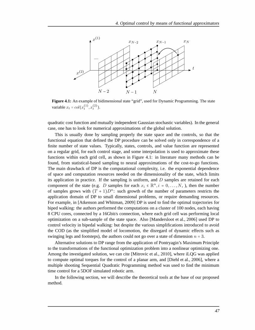
4. Optimal control by means of functional approximators
.......
xN−1xN−2 xNx(1)
x(2)t
NN − 1N − 2Figure 4.1: An example of bidimensional state “grid”, used for Dynamic Programming. The state
variablext = col(x(1)t , x(2)t ).
quadratic cost function and mutually independent Gaussianstochastic variables). In the generalcase, one has to look for numerical approximations of the global solution.
This is usually done by sampling properly the state space andthe controls, so that thefunctional equation that defined the DP procedure can be solved only in correspondence of afinite number of state values. Typically, states, controls,and value function are representedon a regular grid, for each control stage, and some interpolation is used to approximate thesefunctions within each grid cell, as shown in Figure 4.1: in literature many methods can befound, from statistical-based sampling to neural approximations of the cost-to-go functions.The main drawback of DP is the computational complexity, i.e. the exponential dependenceof space and computation resources needed on the dimensionality of the state, which limitsits application in practice. If the sampling is uniform, andD samples are retained for eachcomponent of the state (e.g.D samples for eachxi ∈ Rn, i = 0, . . . ,N , ), then the numberof samples grows with(T + 1)Dn: such growth of the number of parameters restricts theapplication domain of DP to small dimensional problems, or require demanding resources.For example, in [Atkenson and Whitman, 2009] DP is used to findthe optimal trajectories forbiped walking: the authors performed the computations on a cluster of 100 nodes, each having8 CPU cores, connected by a 16Gbit/s connection, where each grid cell was performing localoptimization on a sub-sample of the state space. Also [Mandersloot et al., 2006] used DP tocontrol velocity in bipedal walking: but despite the various simplifications introduced to avoidthe COD (as the simplified model of locomotion, the disregardof dynamic effects such asswinging legs and footsteps), the authors could not go over astate of dimensionn = 3.
Alternative solutions to DP range from the application of Pontryagin’s Maximum Principleto the transformations of the functional optimization problem into a nonlinear optimizing one.Among the investigated solution, we can cite [Mitrovic et al., 2010], where iLQG was appliedto compute optimal torques for the control of a planar arm, and [Diehl et al., 2006], where amultiple shooting Sequential Quadratic Programming method was used to find the minimumtime control for a 5DOF simulated robotic arm.
In the following section, we will describe the theoretical tools at the base of our proposedmethod.
47

4.2 From functional optimization to nonlinear programming
Functional optimization problems deal with the minimization of functionals with respect to ad-missible functions, belonging to infinite-dimensional spaces. Under general hypotheses, theseproblems cannot be solved analytically, however it is possible to provide arbitrarily accuratesuboptimal solutions by solving a suitable approximate nonlinear optimization problem. In thefollowing one of this methods, the Extended RItz Method (ERIM), is described.
4.2.1 Stochastic functional optimization problems
The general formulation of a functional optimization problem is:
Problem 3. Findinfγ∈SF(γ) = inf
γ∈SEzJ [γ, z] (4.1)
whereγ ∈ S are the admissible solutions to the problem, beingS the subset of an infinite-dimensional real normed linear spaceH of functionsγ ∶ B ⊆ Rn ↦ R
m; F ∶ S ↦ R is a costfunctional, whileJ ∶ Rm × Z ↦ R is a given cost function; finallyz ∈ Z ⊆ R
p is a randomvector taking values from a known setZ with a known distribution, setting the problem in astochastic context.
The target of Problem 3 is to find the optimal solutionγ among the admissible functionsγ ∈ S, that minimizes the cost functionalF(γ). The method described hereinafter is statedwithin a stochastic environment, however it can be applied also in deterministic situations. Thestochastic formulation is more complex but is necessary in the presence of random variablesacting on the system, which must be comprised in the problem formulation (e.g. noise, initialor final states with a probability distribution).
The solution of this class of problems is not easy. The analytical computation of the op-timal solution of Problem 3 is feasible in few cases, again principally under LQG conditions.In all the other situations, since finding the analytical solution is hard, it is possible to usenumerical techniques to approximate the desired optimal functions. The principal difficulty isthat in functional problems the goal is to find one or more specific functions over an infinitedimension space:γ = argminF(⋅). Further complications arise in presence of functionaldependencies: anticipating later discussions, if two or more functions must be found, e.g.γ1, γ2 = argminF(γ1, γ2) and there exists a functional dependency, e.g.γ2 = γ2(γ1), thenthey must be found jointly, i.e. they cannot be decoupled. Anusual approach to functionaloptimization is to constrain the solution to take on some structure (e.g. searching for linearsolutions only), so that to obtain a suboptimal solution butthat can be expressed in a simplerand closed form. Other approaches consists in giving up searching for global solutions andstop at local ones, after simplifying the problem, or aimingat the global solution via numericalapproximations, using parameterized functions.
There are several ways to solve such optimization problems by means of functional ap-proximation: the method proposed for this work constrains the functions to take on a fixedstructure with a finite but sufficiently large number of free parameters. By substituting theseparameterized functions in the cost functional and in the constraints expressed by the subset
48
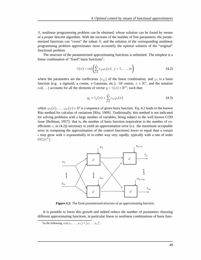
4. Optimal control by means of functional approximators
S, nonlinear programming problem can be obtained, whose solution can be found by meansof a proper descent algorithm. With the increase of the number of free parameters, the param-eterized functions can “cover” the subsetS, and the solution of the corresponding nonlinearprogramming problem approximates more accurately the optimal solution of the “original”functional problem.
The structure of the parameterized approximating functions is unlimited. The simplest is alinear combination of “fixed” basis functions1:
γ(x) = col( ν∑i=1
cijϕi(x), j = 1, . . . ,m) (4.2)
where the parameters are the coefficientscij of the linear combination, andϕi is a basisfunction (e.g. a sigmoid, a cosine, a Gaussian,etc.). Of course,x ∈ Rn, and the notationcol(. . .) accounts for all the elements of vectory = γ(x) ∈ Rm, such that:
yj = γj(x) = ν∑i=1
cijϕi(x) (4.3)
whereϕ1(x), . . . , ϕν(x) ∈H is a sequence of given basis function. Eq. 4.2 leads to the knownRitz method for calculus of variations [Ritz, 1909]. Traditionally, this method is not indicatedfor solving problems with a large number of variables, beingsubject to the well known CODissue [Bellman, 1957]: that is, the number of basis function(equivalent to the number of co-efficientsci in (4.2)) necessary to yield an approximation error (i.e. the maximum acceptableerror in computing the approximation of the control functions) lower or equal than a certainε may grow withn exponentially or in either way very rapidly, typically witha rate of orderO(1/εn).
ϕ
ϕ
ϕ
ϕ
x1
xn
κ1
κν
κν+1
κν+m
γ1
γm
Figure 4.2: The fixed parametrized structure of an approximating function.
It is possible to lower this growth and indeed reduce the number of parameters choosingdifferent approximating functions, in particular linear or nonlinear combinations of basis func-
1In the following,col(x1, . . . , xn) ≜ [x1 . . . xn]⊺.
49

tions containing free parameters (instead of fixed basis functions), in the form:
γ(x,w) = col (γj(x,wj), j = 1, . . . ,m) (4.4)
where
γj(x,wj) = ϕν+j(ϕ1(x,κ1), . . . , ϕν(x,κν), κν+j), j = 1, . . . ,m (4.5)
as shown in Figure 4.2.
Remark 2. The following must be remarked:
• the hidden layer containsϕi, i = 1, . . . , ν, while the output layerϕi, i = ν +1, . . . , ν +m;• the subscripti denoting eachγi is used to disambiguate the basis functions, which in
principle can be of different type; generally, all the functions in a layer adopt the samebasis function homogeneously, for example, one can have a linear output layer and asigmoidal hidden layer (in that case, it is simply said that the OHL-NN has sigmoidalbasis functions);
• for a generic basis functionϕ(⋅, κ), κ ∈ RK is the generic vector containing the freeparameters;K = dim(κ) depends on the basis function type, for example ifϕ(x,κ) =c⊺x + b, thenκ = col(c1, . . . , cn, b) ∈ Rn+1;
• w = col(κi; i = 1, . . . , ν +m) ∈ RW is the big vector of parameters to be optimized, withW = ∑ν+m
i=1 dim(κi);• Eq. 4.4 is a two-layer NN, which is known to be a universal functional approximator
[Hornik et al., 1989], i.e., there are conditions which state the existence of a sufficientnumber of neural units and of the corresponding optimal vector of parameters, givena desired accuracy in approximation. In general, continuous functions can be approx-imated to any degree of accuracy on a given compact set by feedforward NN based onsigmoidal functions, provided that the numberν of neural units is sufficiently large. Thenif the functionγ(x) is unique, and is a continuous functionC(X,Rn), for everyε > 0there exist an integerν and a weight vectorw (and a corresponding “neural” functionγν(x,w)) such that∥γ(x) − γν(x,w)∥ < ε, ∀x ∈ X. Of course, multi-layer NN can beused, guaranteeing further approximation capabilities but at the cost of a larger numberof parameters.
Common basis functions are parameterized splines, sigmoidal or radial basis functions.Using (4.4) instead of (4.2), the number of parameters to be optimized grows “moderately”(polynomially or even linearly) withn. The latter choice leads to the so-calledExtendedRItz Method(ERIM), which was first formalized in [Zoppoli et al., 2002],and refined un-til [Zoppoli et al., 2011]. The theoretical aspects discussing the fundamental property of thepolynomial growth ofW with respect ton and the approximating properties of the methodwere discussed in [Kurkova and Sanguineti, 2005], as long as the concept ofP -optimizing se-quences, which will be introduced later on. The ERIM has proven to be effective in the solutionof functional approximation problems in a variety of context and conditions, with stochasticconstraints/costs, binary signals, linear and nonlinear systems.
50

4. Optimal control by means of functional approximators
4.2.2 The Extended RItz Method (ERIM)
The ERIM basically consists in constraining the admissiblecontrol functionγ(x) ∈ H fromProblem 3 to take on a suitable parameterized but fixed structure γ(x,w) ∈ S, as in Eq. 4.4,with a certain number of free coefficientsw ∈ RW .
The most common structure with the ERIM is aOne-Hidden-Layer Neural Network(OHL-NN), with the following form:
y = γ(x,w) = col( ν∑i=1
cijϕ(x,κi) + bj , j = 1, . . . ,m) (4.6)
where:
• w ∈ RW collects all the parameters to be optimized:w = col (cij ,κi ,bj); i =1, . . . , ν; j = 1, . . . ,m; cij , bj ∈ R, κi ∈ RK ; thenW = νK +m(ν + 1);
• x ∈ Rn, y ∈ Rm so thatγ ∶ Rn ×RW ↦ Rm;
• ϕ ∶ Rn × RK ↦ R are theparameterized basis function(i.e. fixed structure, variableparameters)
Incidentally,γ ∶ Rn ×RW ↦ Rm describes a OHL-NN with linear output layer, whereν ∈ Z+
is the number of “neurons” constituting the network (i.e. the number of “neural units” in thehidden layer) and(ν + m) the total number of “neural units”.ν is also calledcardinalitynumber of the OHL network. W is the finite number of free parameters, and grows linearlywith ν: W = νK +m(ν + 1). The main approximation properties of OHL-NN are discussedin [Hornik et al., 1989, Barron, 1993].
A common structure for the basis functionϕ is theperceptron, represented in Figure 4.3.A perceptron unit consists of a linear combination ofx, where each variable elementxi ismultiplied by a so-called “weight” (i.e. a varying coefficient), plus a bias coefficient, and theirsum is processed by a so called “activation function”.
Remark 3. Except for the additional biasbj , the main difference between (4.6) and (4.4) isthat the sequence of basis functionsϕ0, . . . , ϕν in the hidden layer (where subscripti meantthat each could have a different structure) has been replaced with a set ofν parameterizedbasis function, each of the same type. The reason is that by increasing the cardinalityν we canavoid using different functions if the combination of the simple parameterized basis functionsϕ(⋅, κi) ∈ H,∀κi ∈ Rk has “sufficient” approximation properties. Choosing the most appro-priate OHL networks is crucial: for example, when approximating the solution of Problem 3,generally nonlinear OHL networks require fewer parametersto be optimized with respect tolinear ones (the approximating accuracy being equal).
Sometimes (4.6) is enriched, for example it can have an activation function in the outputlayer different from a simple linear combination of the signals from the hidden layer with a
51

yp = σ(zp)x1
xq
xn
1
wp0
wp1
wpq
wpn
σ
zp
Figure 4.3: A perceptron neural unit, precisely thep-th in the hidden layer of a OHL-NN. Here,σ is the “activation function” of the unit (e.g. a sigmoid),w is a generic “weight”,x is the inputvector to NN, whiley is the output of the hidden layer. A perceptron can be also thebase unit forthe output layer of a OHL-NN: in that case,yp = γp(x,wp), while x (in the figure) is the vectorcoming from the hidden layer.
bias, as anticipated in Remark 22.3
In practical implementations, Eq. 4.6 can be further slightly different. To keep the formu-lation as clear as possible, two important operations have been omitted from the equation (butwill be discussed later on): the input and output normalization functions, i.e. the mappingsMx,My for the range of the variables fed to the NN and exiting the NN is within the range[−1,1]. Using sigmoidal as activation functions ,γ is consequently adapted so that it complieswith the constraints on its admissible values:
γ(x,w) = col(σj [ ν∑h=1
chjσ(x, κh) + bj] , j = 1, . . . ,m) (4.7)
where the notationsσ andx account for the output and input normalization: the input variablesx are normalized from their original range to[−1,1], while the NN outputs are scaled from[−1,1] (the output range of a sigmoidaltanh-based neural network) to the admissible rangeof γ(x). A graphical representation of the OHL-NN in that case is shown in Figure 4.4. Thisoperations are particularly useful whenx andy = γ(x) have a physical meaning, as will beclear in Chapter 5.
Common choices for the parameterized basis functionsϕ(x,κi) are:
2Sometimes a sigmoidal output layer (instead of a classical linear output layer) is preferred since it naturallygenerates bounded values within a specific range, which can be made consistent with the real output ranges afterdata normalization. This choice allows removing signal constraints and not taking care of the possibility that theNN generates inconsistent values.
3It must be noted that the use of OHL-NN is particularly convenient, for its simplicity and for the theoryassessing their approximation properties. However, NN with more than two layers can be used –the so calledmulti-layer NN – which in general may behave even better.
52

4. Optimal control by means of functional approximators
ϕ
ϕ
x1
xn
x1
xn
κ1
κν
c11
cν1
c1m
cνm
b1
bm
z1
zm
σ
σ
y1
ym
y1 = γ1
ym = γm
My1
Mym
Mx1
Mxn
Figure 4.4: A OHL network with normalized input/output. The normalization blocks are put inevidence (magenta and yellow), and the normalized variables are put in evidence by the notationx, y. Single “neural” units (green boxes) as well as the parameters to be optimized (blue text) arealso highlighted.
• radial constructions:ϕ(x,κi) = h(∥x − τi∥2Γi
),where∥x∥2
Γi= x⊺Γix, Γi = Γ⊺i ,Γi > 0, while κi = col(τi, non-redundant elements of
Γi); an example is represented by Gaussian functions, likee−∥x−τi∥
2
Γi ;• ridge constructions:
ϕ(x,κi) = h(α⊺i x + βi),whereκi = col(αi, βi), with βi ∈ R, αi ∈ Rn; moreover,h ∶ R ↦ R can be a linearfunction (such that, e.g.,h(x⊺αi + βi) = x⊺αi + βi) or a nonlinear function, e.g. asigmoidal one4. Feedforward neural networks with one hidden layer and linear activationfunctions are also ridge constructions.
Remark 4. Sometimes to simply the output normalization (My) a common choice is to choosea NN with sigmoidal output layer, for example using
ϕ(z) = ez − e−z
ez + e−z. (4.8)
4Sigmoidal functions are continuous, differentiable, real-valued functions with a “S” shape and the followingproperties: lim
z→+∞σ(z) = 1, lim
z→−∞σ(z) = 0/ − 1. The most common “sigmoid” is the logistic function
σ(z) =1
1 + e−z
defined within[0,1]. Another sigmoidal function, frequently used in NN, is the hyperbolic tangent
tanh(z) =ez − e−z
ez + e−z
defined within[−1,1].
53

which intrinsically generates bounded values within the range[−1,1]. Then, ifγ must generateadmissible values within the range[−U,U], it is straightforward to multiply the output of theNN byU to obtain the desired.5.
Solution to nonlinear programming problems
By substitutingγ(x) with γ(x,w) in Eq. 4.1, the functionalF(γ) becomes a function of afinite number (W ) of parameters:
F(w) ≜ F(γ(⋅,w)) (4.9)
Therefore the original functional optimization problem isturned into a nonlinear programmingone, which can be solved by means of some nonlinear programming descent algorithm. Inparticular, by substituting (4.6) withν = 1,2, . . ., a sequence of “approximating nonlinearproblems” is obtained, each of them defining a nonlinear programming problem equivalent toProblem 3 and defined by the cardinalityν:
Problem 4. Findinfw∈ΨF(w) = inf
w∈ΨEzJ [w,z] (4.10)
wherew ∈ Ψ ⊆ RW ,W = W (ν) is the vector of admissible parameters, related to the con-
straints ofS: Ψ ≜ w ∶ γ(⋅,w) ∈ Aν ∩ S.In order to define the conditions for which the nonlinear programming problem can “ap-
proximate” the functional optimization one, i.e. the parameterized solution approximates thefunctional one, some properties ofF and some conditions must hold.
Assumption 5. An optimal solutionγ to Problem 3 exists, and the infimum and minimum arecoincident:
γ = argminγ∈SF(γ), F = F(γ)
Assumption 6. An optimal solutionw to Problem 4 exists, and the infimum and minimum offunctionF(w) are coincident and attained forw:
w = wν = argminw∈ΨF(wν), F = Fν = F(wν), γ = γν = γ(⋅,wν)
Note thatν is explicit inw = wν , F = Fν and γ = γν to make evidence of the depen-dence on a particular cardinality numberν; but the subscriptν can be dropped whenever theoptimal parameterized solution is intended and it is not necessary to clarify which particularνis used. Moreover, the following properties are required:
5The guarantee of admissible outputs is fundamental when themethod is exploited for generating controls for areal physical platform like a humanoid robot, where unpredictable or wrong controls could damage the system theenvironment, the robot itself or, the worst, people interacting with it.
54
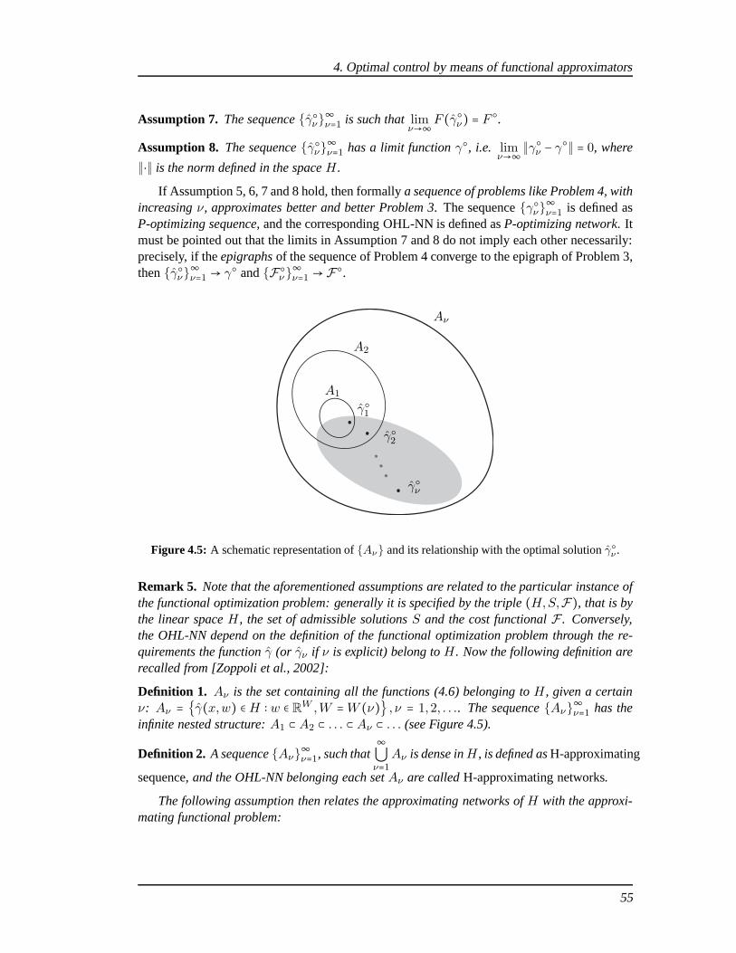
4. Optimal control by means of functional approximators
Assumption 7. The sequenceγν∞ν=1 is such thatlimν→∞
F (γν) = F .Assumption 8. The sequenceγν∞ν=1 has a limit functionγ, i.e. lim
ν→∞∥γν − γ∥ = 0, where
∥⋅∥ is the norm defined in the spaceH.
If Assumption 5, 6, 7 and 8 hold, then formallya sequence of problems like Problem 4, withincreasingν, approximates better and better Problem 3. The sequenceγν∞ν=1 is defined asP-optimizing sequence, and the corresponding OHL-NN is defined asP-optimizing network. Itmust be pointed out that the limits in Assumption 7 and 8 do notimply each other necessarily:precisely, if theepigraphsof the sequence of Problem 4 converge to the epigraph of Problem 3,thenγν∞ν=1 → γ andFν∞ν=1 → F.
.
..
. . .
γ1
γ2
γν
A1
A2
Aν
Figure 4.5: A schematic representation ofAν and its relationship with the optimal solutionγν .
Remark 5. Note that the aforementioned assumptions are related to theparticular instance ofthe functional optimization problem: generally it is specified by the triple(H,S,F), that is bythe linear spaceH, the set of admissible solutionsS and the cost functionalF . Conversely,the OHL-NN depend on the definition of the functional optimization problem through the re-quirements the functionγ (or γν if ν is explicit) belong toH. Now the following definition arerecalled from [Zoppoli et al., 2002]:
Definition 1. Aν is the set containing all the functions (4.6) belonging toH, given a certainν: Aν = γ(x,w) ∈H ∶ w ∈ RW ,W =W (ν) , ν = 1,2, . . .. The sequenceAν∞ν=1 has theinfinite nested structure:A1 ⊂ A2 ⊂ . . . ⊂ Aν ⊂ . . . (see Figure 4.5).
Definition 2. A sequenceAν∞ν=1, such that∞⋃ν=1
Aν is dense inH, is defined asH-approximating
sequence, and the OHL-NN belonging each setAν are calledH-approximating networks.
The following assumption then relates the approximating networks ofH with the approxi-mating functional problem:
55

Assumption 9. The decisional functionγ ∈ S benefits by certain regularity properties so that∞⋃ν=1
Aν is dense inS and the correspondingH-approximating sequence exists.
Of course, this assumption is not sufficient to guarantee theexistence of aP -optimizingsequence. Indeed, the existence ofH-approximating sequences only ensures that an optimalsolution to Problem 3,γ, is an accumulation point for “some” sequenceγν∞ν=1, not neces-sarily for theγν∞ν=1 determined by ERIM after solving a sequence of Problem 4.
The convergence properties of the P-optimizing sequences are fundamental to establish thecomplexity of the method. If the convergence speed of the sequencesF(γν) −F∞ν=1 andγν) − γ∞ν=1, that is the speed at which the optimal solutions of a sequence of Problem 4,with ν = 1,2, . . . epi-converge to the optimal solutions of Problem 3, can be described by:
∃p, q, p′, q′ ∈ R+ ∶ F(γν) −F ≤ O (np
νq) , ∥γν − γ∥ ≤ O (n
p′
νq′ )
then given an approximation accuracyε it is sufficient to choose a cardinality numberν satis-fying:
∃c, c′ ≥ 0 ∶ F(γν) −F ≤ cnp
νq≤ ε, ∥γν − γ∥ ≤ c′n
p′
νq′ ≤ ε
to have
ν ≥max
⎡⎢⎢⎢⎢⎣(cε)
1
q
np
q ,(c′ε)
1
q′
np′
q′
⎤⎥⎥⎥⎥⎦. (4.11)
If a P-optimizing sequence verifies (4.11), then it is calledpolynomially complex P-optimizingsequence, as given the maximum approximation errorε (for whichF, γ are approximated)the basis cardinality numberν grows at most as a power ofn, which is the input dimensionof the OHL-NN, hereby calledpolynomially complex P-optimizing network. The existence ofa polynomially complex P-optimizing sequence makes the approximate solution of Problem 3computationally feasible, and by (4.11) ensures that it is possible, by acting onν, to obtain anydesired degree of accuracy in the approximation by using networks containing a suitable butmoderate number of parameterized basis functions.
Remark 6. The polynomial growth ofν in the ERIM is a fundamental improvement withrespect to the equivalent of the classical Ritz, where typically the growth is in the order ofO(1/εn). In literature many limitations of the latter method are reported, the major beingthe inability to deal with the setS of admissible functions depending on a large number ofvariablesn, and the consequent COD. Furthermore, the known error estimates (for the Ritzmethod) either refer to the casen = 1 or provide upper bounds which do not make explicitthe dependence onn: hence, it is unclear to which extent it is possible to obtainarbitrarilyaccurate approximations by means of a “moderate”ν when the admissible decision functionsγ depend on a large numbern of variables.
The upgrade of the approximating functions (from linear to nonlinear basis ones) is the keyof the ERIM, which makes it avoid the COD. Several kinds of approximating networks behave
56

4. Optimal control by means of functional approximators
like “polynomially complexH- approximating networks”, if the functions to be approximatedattain some regularity conditions. In particular, for various triple(H,S,F) it has been shownthat a proper sequence of OHL-NN can be constructed by minimizing the functional overS ∩Aν : the resulting is polynomial complex P-optimizing sequence. To this extent, the functionalF must exhibit the properties of continuity and convexity. More discussions on the convergencerates in this case can be found in [Kurkova and Sanguineti, 2005, Krurkova, 1997], where theupper bounds of the rates are found: the interesting property is that the errorF(γν) −F(γ)(both when the cost functionalF is continuous only and continuous and uniformly convex) isbounded by a quantity which is at least inversely proportional to ν1/2, thus independently onn. Notwithstanding, a largeν is not sufficient alone to lower the approximation error, as itsupper bound is also proportional to the variation norm of theoptimal solution,∥γ∥Gn
ϕ, being
Gnϕ ≜ ϕ(⋅, κ) ∶ κ ∈ Rk is the set of functions that can be obtained by varying the free parameters
in the basis functionsϕ. That is, the norm is related to the basis functionsϕ in the OHL-NNand can be estimated if some a-priori knowledge on the admissible solutions is available. Itis important to remark that the conditions which allow constructing the polynomially complexsequences, regard the functionalF and the set of admissible functionS, and are specifiedby geometric and regularity properties stated in a “static”context: a dynamic system evolvingduring the optimization process is not taken into account, or, if it exists, is implicitly consideredand embedded in the properties ofF andS.
4.2.3 A stochastic approximation technique
Problem 4 can be solved by means of a classical gradient technique, if the following funda-mental assumption regardingJ (see Eq. 4.10) is verified:
Assumption 10. J (w,z) is aC1 function with respect tow, ∀z.
In the following, the various constraints onw, which define the setΨ ∶ w ∈ Ψ, are takeninto account through penalty functions, so that Problem 4 isreduced to an unconstrained non-linear programming problem. If “exact” constraints onw must be fulfilled, there exist specificstochastic approximation techniques that can handle them as required [Kusher and Yin, 1997].If Assumption 10 is verified, then under some additional regularity hypotheses alsoF(w) is aC1 function, thus its gradient can be computed, i.e. all the partial derivatives ofF with respectto the parametersw. Then, it is possible to compute the set of optimal parametersw by meansof a classical nonlinear programming technique.
Among classical nonlinear programming algorithms, we focus our attention on gradientalgorithms to introduce the concept of stochastic approximation in a simple and straightforwardway. A general gradient descent algorithm is in the form
w(k + 1) = w(k) + α(k)s(k), k = 0,1, . . . (4.12)
wheres(k) is a generic descent direction, andα(k) is a positive step-size. The idea of gradientmethods is to exploit the derivative of the cost functionJ (w) to find its minimum, attained atw, where∇J (w) = 0. A descent directions(k) satisfies the condition∇J (w(k))⊺s(k) <0. The numerical procedure consists in starting from a guess or a random realization of the
57

parameters,w(0), to generate a sequence of parameters valuesw(1),w(2), . . . ,w(k),w(k+1)which satisfiesJ (w(k)) > J (w(k+1)). Typical examples of gradient descent algorithms are:
• Steepest Descent:w(k + 1) = w(k) −α(k)∇J (w(k))• Newton:w(k + 1) = w(k) −α(k)[∇2J (w(k))]−1∇J (w(k))• Quasi-Newton:w(k + 1) = w(k) − α(k)D(k)∇J (w(k)), whereD(k) is an approxi-
mation of the Hessian
Incidentally, it must be noticed that the aforementioned algorithms are designed for a numericalapproximation based on a deterministic gradient,∇J . In our case, the gradient is stochastic,becauseF = E J . In this case, the stochastic gradient (which is particularly tough to com-
pute) can be substituted by its numerical approximation, and specifically by the gradient whichis computed if a single realization of the stochastic variable occurs. Without going into furtherdetails of the algorithms, we will bring forward with our discussion using the steepest descentalgorithm, that turns out to be the best choice for this problems [Spall, 2003].
The iterative steepest descent algorithm which allows solving Problem 4 is:
w(k + 1) = w(k) −α(k)∇w EzJ (w(k), z) , k = 0,1, . . . (4.13)
Due to the general assumptions of Problem 4, it is practically impossible to compute an-alytically the gradient∇wE
zJ (w(k), z): indeed, at each iteration stepk, the gradient of a
complex function resulting from a multiple integral, related to the stochastic properties ofz.Stochastic approximation, applied to overcome such computational difficulties, consists in
using∇wJ [w(k), z(k)] i.e. the gradient computed after a single realization of thestochasticvariablez. Thus, instead of (4.13), the following updating algorithmis used:
w(k + 1) = w(k) − α(k)∇wJ [w(k), z(k)] , k = 0,1, . . . (4.14)
where the sequencez(k) is generated randomly according to the known probability distri-bution ofz. α(k) is a suitably decreasing positive step-size. The convergence of thestochasticgradientmethod is assured by a particular choice of the step sizeα(k), that must fulfill a setof conditions [Kushner and Yang, 1995].
Remark 7. If J (w,z) is continuous and differentiable (see Assumption 10), under some reg-ularity hypotheses alsoE
zJ (w,z) is, and:
∇wEzJ (w,z) = E
z∇w [J (w,z)] . (4.15)
In practical situations, this formula can be exploited to have a certain “rough” approximationof the stochastic gradient to be used in place of the single realization∇wJ [w(k), z(k)], i.e.
Ez∇w [J (w,z)] ≈ 1
Q
Q∑q=1
∇w [J (w,z(q))] . (4.16)
By increasing suitably the number of realizationsQ to consider at each iteration stepk, it ispossible to obtain a better approximation of the original gradient. This approach has been
58

4. Optimal control by means of functional approximators
used, for example, in [Ivaldi et al., 2008b], and similarly in [Ivaldi et al., 2009a] for the eva-luation of a stochastic constraint. Of course the additional computational burden of such ap-proximation with respect to the “single” stochastic approximation approach must be balancedwith the improvement in the descent accuracy. This solutionmust be also balanced with thestrategy for the adaptive step-sizeα(k), which is often “perturbed” as being the main objectof heuristics like simulated annealing: since the gradientis already “perturbed” (even if aver-aged onQ realizations as in Eq. 4.16), sometimes it is difficult to assess if the gradient or thestep-size are determinant for the convergence of the algorithm (4.13).
Eq. 4.14 is the simplest stochastic approximation method. Among the sufficient conditionsfor its convergence, which can be found in [Kusher and Yin, 1997], some concern the “shape”of the cost surfaceF(w) (but are very difficult to assess due to the characteristics of the surfaceitself), some the decreasing behavior ofα(k). [Baglietto, 1998] the convergence requisites arediscussed. In particular, if functionF(w) andα verify the following assumptions:
• F(w) ≥ 0,∀w ∈ RW ;• F(w) is continuous and differentiable, and a Lipschitz constantL exists such that∥∇F(w)−∇F(w′)∥ ≤ L ∥w −w′∥ , ∀w,w′ ∈ RW ;
• ∃c ∈ R+ ∶ ∇F(w(k))⊺ E [s(k)∣Is(k)] ≥ c ∥∇F(w(k))∥2 , k = 0,1, . . ., wheres(k)is a certain descent direction in (4.12) andIs(k) ≜ [s(k − 1), . . . , s(0),w(k − 1), . . . ,w(0)];
• ∃K1,K2 ∈ R+ ∶ E [∥s(k)∥2 ∣Is(k)] ≤K1 +K2 ∥∇F(ω(k))∥2 , k = 0,1, . . .;• the sequence of step-sizesα(k) > 0 also satisfies:
∞∑k=0
α(k) =∞ ,∞∑k=0
α2(k) <∞then:
• the sequenceF(w(k)) converges;• lim
k→∞∇wF(w(k)) = 0;
• any limit pointw in sequencew(k) is stationary, and∇wF(w(k)) = 0.
Of course, the properties ofF(w(k)) are related to the ones ofJ . With regard to thestep-size properties, it is requested thatα(k) decreases towards zero with the increase of theiterationsk: this is necessary since at the convergence pointw it could happen thats(k) ≠ 0(even if the exact gradient is null, as a consequence of the stochastic approximation). It is butnecessary that the stepsize does not become too “small” too soon, to avoid the risk that thealgorithm could be stucked in some local minima, and not be able to move out of it.
Example 1. If s(k) < b and∞∑k=0
α(k) ≤ B <∞, then∥w(k) −w(0)∥ ≤ ∑k−1i=0 α(i) ∥s(i)∥ ≤
bB,k = 1,2, . . ., that isw(k) is confined into a ball of radiusbB and centerw(0): if theoptimal solution was outside that ball, the algorithm wouldnever reach that and eventuallystop in a local minima. This motivates why the step-size can be neither constant nor too small.
59

A step-size satisfying the aforementioned conditions (andwidely used because of its sim-plicity) is:
α(k) = c1
c2 + k, c1, c2 > 0. (4.17)
In literature different techniques have been suggested to accelerate the algorithm’s conver-gence; in particular,ad hocmethods exists to optimize the neural networks’ parameters. Itis necessary to point out that heuristics frequently improve the optimization process, but theirconvergence and performance cannot be generally proveda priori.
4.2.4 Team functional optimization problems
Whenever a plurality of unknown functions is considered, Problem 3 must be extended. Let usconsider a team withM agents orDecision Makers(DM), whose decisions are expressed bythe functionsγ0, . . . , γM−1. Assuming that each DM can measurexi and use it to compute itsdecisionγi(xi), and that the decisions of the team must minimize a certain global costJ , thefollowing problem can be stated.
Problem 5. Find
infΓ∈SM
F(Γ) = infΓ∈SM
EzJ [γ0(x0), . . . , γM−1(xM−1), z] (4.18)
whereΓ ≜ col (γ0, . . . , γM−1) is the set of functionsγi(xi) ∶ Bi ∈ Rni ↦ Rmi , each belonging
to an infinite-dimensional real normed linear spaceHi, i = 0, . . . ,M −1; SM ⊆H0×H1× . . .×
HM−1 is the subset of admissible functions; each functionγi has a specific argumentxi, whichmay depend onz as well as on the other decision functionsγj, j ≠ i; z ∈ Z ⊆ Rp is a randomvector taking values from a known setZ with a known distribution; finallyF ∶ SM ↦ R is thecost functional, andJ ∶ Rn0 ×Rn1 × . . .RnM−1 ×Z ↦ R.
Examples of Problem 5 are:
• team functional optimization problems, when several decision makers, each provided a“personal” information vectorIi (whereIi = xi or genericallyIi = g(x0, . . . , xM−1)),cooperate to minimize a common cost functional
• T -stage stochastic single-person optimal decision problems, whereM is the number ofcontrol/decision instantsT , and random disturbancesz act on the controlled system
• Finite Horizon control problems, whereM is the number of control instants, randomdisturbancesz represents the noise vector (e.g. the noise acting on the system), whilexi is the generici-th state vector of the system to be controlled: in this case the systemmodel is known and embedded in the problem formulation (transparently in (4.18))
The latter is of particular interest, since it would be the object of our further investigations.
Remark 8. It must be remarked that the argumentsxi may depend onz and other functionsγj , j ≠ i, through known mappings. In fact,xi is often written asIi and called “informationvector”, denoting the aggregation of all the possible information in input to the decision func-tion γi, representing a so-calleddecision maker(DM), or decisional entity. In this cases, it is
60

4. Optimal control by means of functional approximators
useful to have a graphical representation of the information flux among the functionsγi, as afundamental role is played by the “partial nesting” or not ofthe information structure of eachDM [Baglietto et al., 2001b].
The theoretical properties holding true for Problem 3 can befully extended to Problem 5.
4.2.5 Some notes on the optimization phase
The proposed method enables NN to approximate the optimal feedback solutions, and is sup-posed to overcome the COD of DP-based solutions. Certain aspects deserve some attention:
• The optimal solution are approximated numerically, and itis not possible to distinguisha local from the (or a) global solution when running the optimization algorithms; forthe same reason, the stability of the weight update cannot beguaranteed, since a pre-cise analytical condition is missing. The so called “training phase” requires consistentcomputations and a large number of patterns for the training, depending on the problemstatement. Computations are so demanding (in terms of time), that they sometimes pre-vent the use of the solution in real-time applications. In Section 4.5.4 a more detaileddiscussion on such limits is reported.
• NNs have been chosen for their approximating properties. Barron proved that neuralnetworks are universal approximators for continuous functions, more efficient than tra-ditional functional approximators (polynomials, splines, trigonometric expansions, etc.),even though there exists a fundamental bound on the functional reconstruction error[Barron, 1993], which is condensed in Maurey-Jones-Barrons bound. The mean inte-grated squared error between the approximating neural network and the target functionf is bounded by
O⎛⎝C2
f
ν
⎞⎠ +O (
νn
LlnL) (4.19)
whereν is the number of neural units,n is the input dimension of the function,L isthe number of training observations, andCf is the first absolute moment of the Fouriermagnitude distribution of the target functionf [Barron, 1994]. In particular, withν ≈Cf(L/(n lnL))1/2 neural units, the order of the bound on the mean integrated squarederror is optimized to beO(Cf((n/L) lnL)1/2). In [Niyogi and Girosi, 1996], similarresults are shown for Gaussian radial basis functions (RBF)networks, in particular thegeneralization error is bounded by
O (1ν) +O ⎛⎝[
νn ln(νL) − ln δL
]1/2⎞⎠ (4.20)
wheren is the number of inputs,ν the number of neural units,L is the set of trainingobservations, andδ is a positive real number, with0 < δ < 1. A frequent heuristic todetermine an approximation of the optimal number of neural units ν for a given numberof training observationsL is also given byν ∝ L1/3. This result takes into account the
61
compromise between the minimization of the generalizationerror (which would requirehigh numbers ofν) and of the estimation error (which would require a low number ofL). As a rule of thumb, in other works (for example [Barambonesand Etxebarria, 2002])reasonably good results are usually obtained if the number of neural units is roughly two-three times the order of the system. Since in our framework the functions to approximateare the unknown, it is not possible to make any guess, in particular onCf (Eq. 4.19).The underlying assumption is that an optimal set of parameters exists, given a desiredapproximation error. In practical terms, multiple trainings are usually performed, andthe number of neurons is “manually” adjusted .
• A two-layer (or One-Hidden-Layer) neural network can be used to approximate any non-linear function, with a suitable number of neural units. In [Nguyen and Widrow, 1990]a method is proposed for the initialization of the weights inorder to reduce the trainingtime. The basic idea is that picking initial weights so that the hidden units are scatteredin the input space substantially improves learning speed ofnetworks with multiple in-puts. In the following formulation, the elements of the input vector (xt for example) takevalues from the range[−1,1] (the so calledinput normalization). Considering the outputy of a OHL neural networks with sigmoidal activation function, y = ∑ν−1
i=0 viσ(xwi + bi)whereν is the number of neurons in the hidden layer, andN is the dimension of the in-put vectorx (sox ∈ Rn), then callingrand(a, b) the operation which extracts a uniformrandom number within a certain range[a, b], weights and biases are randomly initializedin the following way:
∣wi∣ = ν 1
n , bi = rand(− ∣wi∣ , ∣wi∣)The authors in [Nguyen and Widrow, 1990] also suggest that a certain overlap betweenthe intervals must be provided, by setting the magnitude ofwi to 0.7ν
1
n . Nguyen’s for-mulation was proposed for neural networks approximating SISO (Single-Input-Single-Output) and MISO (Multiple-Input-Single-Output) functions. In particular, the exactformula is provided only for the first case, while the latter is “solved” by simply scalingthe range of admissible values with the magnitude. Extensions to the MIMO (Multiple-Input-Multiple-Output) can be easily found. For example, apossible adaptation to themultiple dimension case is to choose weightw and biasb as:
b = urand(0.7ν(1/n)) , w = urand((0.7/n)ν(1/n)) (4.21)
whereν,n are the number of neurons and the number of inputs of the NN, respectively,andurand(a) is a function extracting a random value within the range[−a, a].
• The choice of the approximating functions is critical. Alternatively to NN, one coulduse other functional approximators, like Gaussian MixtureModels (GMM) or SupportVector Machines (SVM). However, there is no trivial way intoapplying SVM in ourcurrent approach. Firstly, SVM is meant as a supervised learning method, i.e. it triesto find a functionf(x,α) (with alpha being it’s parameters) that approximates best aset of labeled samplesS, whereS = (x1, y1), . . . , (xn, yn), wherexi is the i-th inputvector andyi the i-th label (desired output). SVM basically tries to find a solution that
62
4. Optimal control by means of functional approximators
minimizes the error between the predictedy and the actualy, by means of a quadraticoptimization problem, which is convex (hence it yields a single optimal solution). Thisis incompatible with our approach, where there is no such thing as a desired output andtherefore neither an error; there is only the cost functional F . Moreover, the canonicalSVM expects to be trained on a batch of labeled samples, whereas in our method samplesof the stochastic variables are fed into the ’learning’ algorithm one-by-one, after whichthe parameters are updated. A possible setting in which SVM could easily be applied, isif a set of optimal control commandsut would be known for a given set of input vectorsxt, so that a certain training set could be created, and the SVM could then be trained onthis set of labeled samples.
4.3 Finite and Receding Horizon control problems
4.3.1 Applying the ERIM to solve aT -stage stochastic optimal control problem
In the following the ERIM is applied to the solution of general T -stage stochastic optimalcontrol problem, i.e. a problem where a sequence ofT optimal control functions minimizing acertain cost functional has to be found. Typical problems are the control of teams of cooperatingagents, decisional problems where multiple entities play arole, but more frequently to the FiniteTime or Finite Horizon control.
Here we state aT -stage stochastic optimal control problem, where the goal is to find theT optimal control laws that steer the dynamic system from an initial known statex∗
0to a final
desired onex∗T , by minimizing a suitable cost functionJ .6
Problem 6. Given known boundary conditions, i.e. fixed initial statex0 = x∗0 and final statex∗T to reach inT stages, for the system:
xt+1 = ft (xt, ut, ηt) , t = 0,1, . . . , T − 1 (4.22)
wherext ∈ Xt ⊆ Rn, ηt is a stochastic variable with known distribution, and the controls aresubject to the following
ut = γt (xt) ∈ Ut(xt) ⊆ Rm (4.23)
find a sequence of optimal control functionsγ0(x0), . . . , γT−1(xT−1)minimizing the cost func-
tional
F = Eη0,...,ηT−1
J = Eη0,...,ηT−1
T−1∑t=0
ht(xt, γt (xt)) + hT (xT ) (4.24)
Eq. 4.22 is a set of equations describing a discrete-time stochastic dynamic system (ingeneral, nonlinear), where at the time instantt, xt is the state vector, which may be takingvalues from a finite setXt ⊆ Rn, starting from a known initial statex0 = x∗0 ; ut is an admissiblecontrol vector, constrained to take values from a finite setUt(xt) ⊆ R
m; ηt is an exogenous
6The following is a fundamental problem, addressing the mainaspects of a FH stochastic optimal control prob-lem. The boundary conditions (i.e. fixed initial and desiredstate) but make it unsuitable for RH controls, as will beexplained later on.
63

variables vector.T is a known positive integer. It must be remarked that the constraints (4.23)can be expressed by means of additional penalty functions tobe added to the main cost function,that is turning a hard constraint into a soft one.η0, η1, . . . , ηT−1 are random disturbances,and if Dynamic Programming (DP) was applied to solve the problem later on, the mutualindependence of each random vector would be required. If theERIM is applied, then thisassumption can be removed.
The state vectorxt, at time instantt, is perfectly known or measurable, thus it can be used todesign a feedback control lawut = γ(xt). We remark that a feedback control law is necessarywhenever noise and generally disturbances act on the system, or if we want to counteract tounknown or unmodeled dynamics in the system itself, which could drive it into undesired statesor even compromise its stability. The cost functionJ is generally of the type:
J = T−1∑t=0
ht(xt, ut) + hT (xT ) (4.25)
where the final termhT (⋅) usually weights the disparity between the system state at the end ofthe maneuver and the desired state; and a sum of termsht(⋅), which can weigh the disparitybetween the desired and the system state during the maneuver, the trajectory shape, or theeffects of controls, their consumption etc. Note that because of (4.23),J is a “function offunctions”, and precisely:
J = J (γ0, . . . , γT−1) (4.26)
Eq. 4.25 has a stochastic nature, because the system is affected by noise, so the formulationof the problem takes into account the minimization of the expected value ofJ , i.e. the costfunctionalF = E J .Remark 9. It is important to point out that in Problem 6 the initial system statex0 is fixed tox∗0, because the goal was to find a sequence of controls for specific boundary conditions. The
final statexT is not constrained to take on a desired value, but a desired valuex∗T is specified.Typically, the desired state (i.e. the state to reach) is expressed by penalty functions in the costfunction to be minimized, such as:
hT (xT ) = VT (xT − x∗T )2whereVT ∈ Rn×n, VT = V ⊺T > 0 is a gain matrix weighting each component differently. In thefollowing, we will not explicitly state the dependency of system trajectories, cost function, etc.to the desired final state, to keep all formulas lighter.
It is well known that Problem 6 can be solved “analytically” through the DP only if suitableconditions hold, typically the known LQG hypotheses (linear system, quadratic cost functionand mutually independent Gaussian stochastic variables).In the general case, one has to lookfor approximate solutions. This is usually done by discretizing or sampling properly the statespace and the controls, so that the functional equation thatdefined the DP procedure can besolved only in correspondence of a finite number of state values: for each control stage, auniformly (or not) sampled state space is found (an example was shown in Figure 4.1).
64
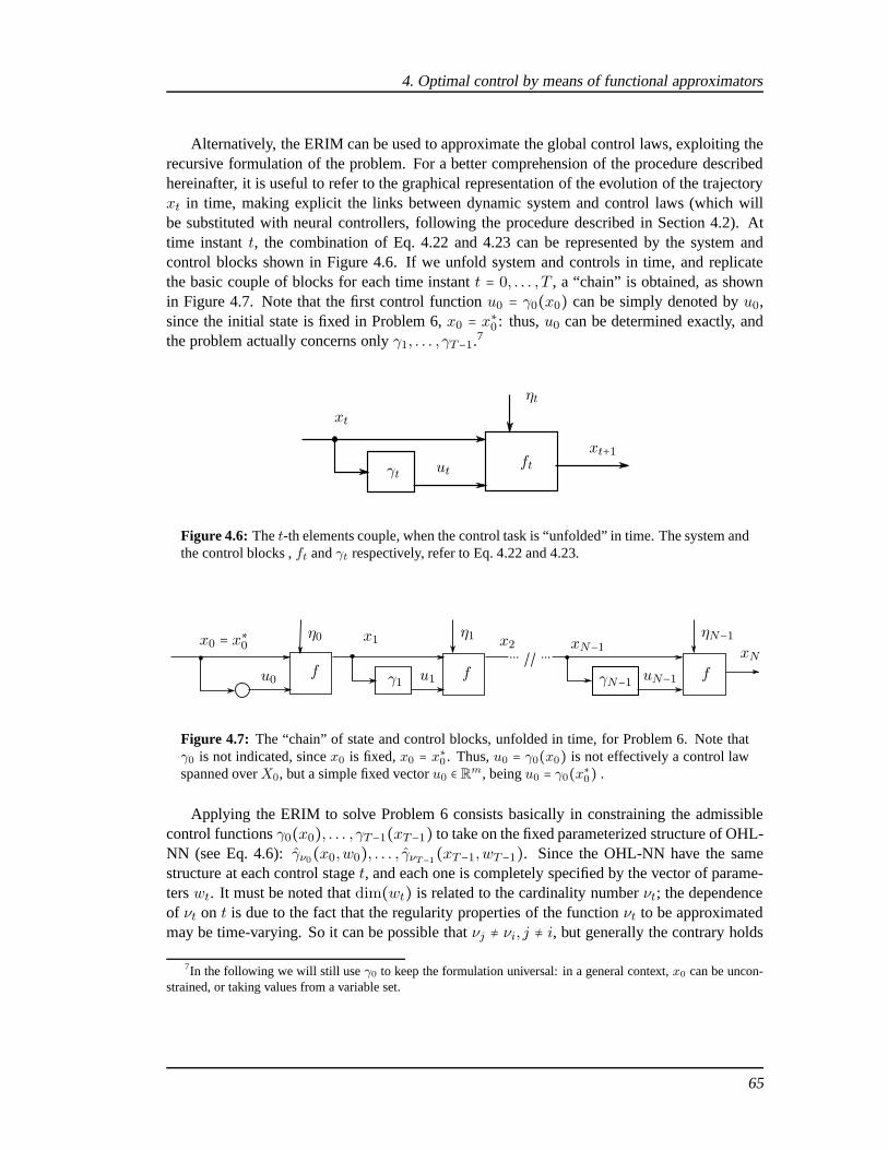
4. Optimal control by means of functional approximators
Alternatively, the ERIM can be used to approximate the global control laws, exploiting therecursive formulation of the problem. For a better comprehension of the procedure describedhereinafter, it is useful to refer to the graphical representation of the evolution of the trajectoryxt in time, making explicit the links between dynamic system and control laws (which willbe substituted with neural controllers, following the procedure described in Section 4.2). Attime instantt, the combination of Eq. 4.22 and 4.23 can be represented by the system andcontrol blocks shown in Figure 4.6. If we unfold system and controls in time, and replicatethe basic couple of blocks for each time instantt = 0, . . . , T , a “chain” is obtained, as shownin Figure 4.7. Note that the first control functionu0 = γ0(x0) can be simply denoted byu0,since the initial state is fixed in Problem 6,x0 = x∗0 : thus,u0 can be determined exactly, andthe problem actually concerns onlyγ1, . . . , γT−1.7
xt
xt+1utγt
ft
ηt
Figure 4.6: Thet-th elements couple, when the control task is “unfolded” in time. The system andthe control blocks ,ft andγt respectively, refer to Eq. 4.22 and 4.23.
x0 = x∗0 η0
u0
x1 η1
u1γ1
x2 // xN−1ηN−1
uN−1γN−1
xNfff
Figure 4.7: The “chain” of state and control blocks, unfolded in time, for Problem 6. Note thatγ0 is not indicated, sincex0 is fixed,x0 = x∗0 . Thus,u0 = γ0(x0) is not effectively a control lawspanned overX0, but a simple fixed vectoru0 ∈ Rm, beingu0 = γ0(x∗0) .
Applying the ERIM to solve Problem 6 consists basically in constraining the admissiblecontrol functionsγ0(x0), . . . , γT−1(xT−1) to take on the fixed parameterized structure of OHL-NN (see Eq. 4.6):γν0(x0,w0), . . . , γνT−1(xT−1,wT−1). Since the OHL-NN have the samestructure at each control staget, and each one is completely specified by the vector of parame-terswt. It must be noted thatdim(wt) is related to the cardinality numberνt; the dependenceof νt on t is due to the fact that the regularity properties of the function νt to be approximatedmay be time-varying. So it can be possible thatνj ≠ νi, j ≠ i, but generally the contrary holds
7In the following we will still useγ0 to keep the formulation universal: in a general context,x0 can be uncon-strained, or taking values from a variable set.
65

xt
xt+1
utγft
ηt
wt
Figure 4.8: Thet-th elements couple of Figure 4.6, after the application of the ERIM. Note thatγtis being approximated byγ(xt,wt). The structure ofγ is fixed, while the control law is completelyspecified bywt.
true, so it is possible to drop the subscriptνt from γ and letwt specify thet-th control function:
ut = γ(xt,wt), t = 0, . . . , T − 1 (4.27)
as shown in Figure 4.8 for thet-th element of the chain. Note again that the first controlfunctionu0 = γ0(x0) does not need to be replaced with the OHL-NN, since the initial state,in this context, is a fixed vectorx0 = x∗0 , but we will still mention it to keep a more generalformulation. Indeed, this is valid only if the initial stateis fixed: if x0 is a stochastic variablewith its own probability density, thenγ0(x0)must be replaced withu0 = γ(x0,w0) as the otherfunctions (becauseu0 obviously depends onx0). This case will be object of interest later on.
By substituting (4.27) in (4.24), the general cost functionJ (the “function of functions” asin (4.26)) is turned into a function which is only dependent on a finite number of real variables:
J (w) = J (u0,w1, . . . ,wT−1) (4.28)
wherew contains all the parameters to be optimized:
w ≜ [u0,w1, . . . ,wT−1] ∈ RW , (4.29)
with W =m +∑T−1i=1 Wi (beingu0 ∈ Rm andwi ∈ RWi).
The solution of Problem 6 by means of the ERIM can be then summarized by these threemain steps:
• write the cost functionalJ (u0, γ1, . . . , γT−1)• substitute the control functions with the OHL-NN:J (u0, γ(⋅,w1), . . . , γ(⋅,wT−1))• write the cost functionJ (u0,w1, . . . ,wT−1)
If the assumption on the known initial statex0 = x∗0 does not hold, the general formulation is:
66

4. Optimal control by means of functional approximators
J (γ0, γ1, . . . , γT−1)
J (γ(⋅,w0), γ(⋅,w1), . . . , γ(⋅,wT−1))
J (w0,w1, . . . ,wT−1)Problem 6 is then turned into the following:
Problem 7. Given known boundary conditions, i.e. fixed initial statex0 = x∗0 and final statex∗T to reach inT stages, for the system (4.22), where the controls are subject to (4.27) find thevectors of optimal parametersw0, . . . ,w
T−1, i.e. w (see Eq. 4.29), which minimize the cost
function
F = Eη0,...,ηT−1
J (w) = Eη0,...,ηT−1
T−1∑t=0
ht(xt, γ(xt,wt)) + hT (xT ) (4.30)
under the constraints given by the state equation.
Gradient algorithms and stochastic approximation
As done for Problem 3- 4, it is possible to approximate progressively better Problem 6, by suit-ably increasing the cardinality number in theT OHL-NNs, with a sequence of unconstrainednonlinear programming problems. In analogy to the solutionproposed for Problem 4, the opti-mal parameters of Problem 7 can be found through a nonlinear programming algorithm and astochastic approximation technique:
w(k + 1) = w(k) −α(k)∇w EηJ (w), k = 0,1, . . . (4.31)
whereη ≜ col(η0, . . . , ηT−1). As already discussed in Section 4.2.3, it is impossible to calcu-late exactly all the gradient components, because of the stochastic nature ofη. A stochasticapproximation technique is then applied and the update equation becomes:
w(k + 1) = w(k) − α(k)∇w(k)J (w, η(k)) k = 0,1, . . . (4.32)
where the sequenceη(0), . . . , η(k), η(k + 1), . . . is generated randomly according to theknown probability density function of eachηi,∀i. Of course, it must be assumed that functionJ(w, η(k)) isC1 with respect tow for all η0(k), . . . , ηT−1(k).
In order to update the value of each parameterwit(k) (the i-th parameter of the vectorwt
at the iteration stepk), the partial derivatives ofJ with respect tow(k)must be computed, i.e.
∂J∂u0(k) ,
∂J∂wt(k) = col(
∂J∂wi
t(k)) , t = 1, . . . , T − 1; i = 1, . . . ,Wt (4.33)
67
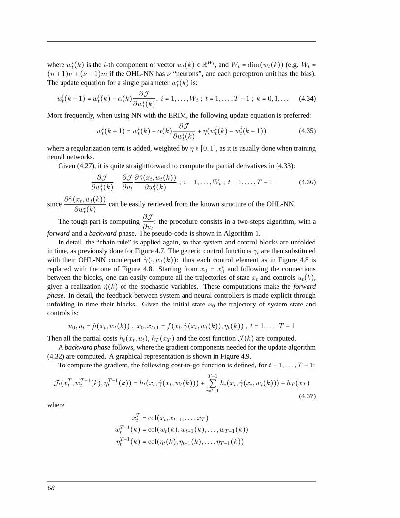
wherewit(k) is thei-th component of vectorwt(k) ∈ RWt, andWt = dim(wt(k)) (e.g.Wt =(n + 1)ν + (ν + 1)m if the OHL-NN hasν “neurons”, and each perceptron unit has the bias).
The update equation for a single parameterwit(k) is:
wit(k + 1) = wi
t(k) −α(k) ∂J∂wi
t(k) , i = 1, . . . ,Wt ; t = 1, . . . , T − 1 ; k = 0,1, . . . (4.34)
More frequently, when using NN with the ERIM, the following update equation is preferred:
wit(k + 1) = wi
t(k) −α(k) ∂J∂wi
t(k) + η(wit(k) −wi
t(k − 1)) (4.35)
where a regularization term is added, weighted byη ∈ [0,1], as it is usually done when trainingneural networks.
Given (4.27), it is quite straightforward to compute the partial derivatives in (4.33):
∂J∂wi
t(k) =∂J∂ut
∂γ(xt,wt(k))∂wi
t(k) , i = 1, . . . ,Wt ; t = 1, . . . , T − 1 (4.36)
since∂γ(xt,wt(k))
∂wit(k) can be easily retrieved from the known structure of the OHL-NN.
The tough part is computing∂J∂ut
: the procedure consists in a two-steps algorithm, with a
forward and abackwardphase. The pseudo-code is shown in Algorithm 1.In detail, the “chain rule” is applied again, so that system and control blocks are unfolded
in time, as previously done for Figure 4.7. The generic control functionsγt are then substitutedwith their OHL-NN counterpartγ(⋅,wt(k)): thus each control element as in Figure 4.8 isreplaced with the one of Figure 4.8. Starting fromx0 = x∗0 and following the connectionsbetween the blocks, one can easily compute all the trajectories of statext and controlsut(k),given a realizationη(k) of the stochastic variables. These computations make theforwardphase. In detail, the feedback between system and neural controllers is made explicit throughunfolding in time their blocks. Given the initial statex0 the trajectory of system state andcontrols is:
u0, ut = µ(xt,wt(k)) , x0, xt+1 = f(xt, γ(xt,wt(k)), ηt(k)) , t = 1, . . . , T − 1Then all the partial costsht(xt, ut), hT (xT ) and the cost functionJ (k) are computed.
A backward phasefollows, where the gradient components needed for the update algorithm(4.32) are computed. A graphical representation is shown inFigure 4.9.
To compute the gradient, the following cost-to-go functionis defined, fort = 1, . . . , T − 1:
Jt(xTt ,wT−1t (k), ηT−1t (k)) = ht(xt, γ(xt,wt(k))) + T−1∑
i=t+1
hi(xi, γ(xi,wi(k))) + hT (xT )(4.37)
where
xTt = col(xt, xt+1, . . . , xT )wT−1t (k) = col(wt(k),wt+1(k), . . . ,wT−1(k))
ηT−1t (k) = col(ηt(k), ηt+1(k), . . . , ηT−1(k))
68

4. Optimal control by means of functional approximators
x0η0
u0
x1 η1
u1γ1
x2 // xN−1ηN−1
uN−1γN−1
xN
fff
∂J∂u0
∂J∂w1
∂J∂wN−1
J
Figure 4.9: Backward phase: the partial derivatives of the cost function with respect to the outputsare back-propagated through the OHL-NNs. Inside each blockγ, the partial derivatives with re-spect to the parameters to be optimized are computed and usedfor the gradient descent. Note thatto simplify the notation and the scheme,γt = γ(⋅,wt).
The partial derivatives with respect to the parameters are then, fort = 1, . . . , T − 1:
∂Jt∂wt(k) =
∂ht(xt, ut)∂ut
∂γ(xt,wt(k))∂wt(k) +
+∂Jt+1(xTt+1, uT−1t+1 , ηT−1t+1 (k))
∂xt+1
∂ft(xt, ut, ηt(k))∂ut
∂γ(xt,wt(k))∂wt(k) (4.38)
whereas for the first control, fixed, beingu0 = γ(x∗0):∂J0∂u0
= ∂h0(x0, u0)∂u0
+∂J1(xT1 , uT−11 , ηT−11 (k))
∂x1
∂f0(x0, u0, η0(k))∂u0
(4.39)
Exploiting the chain rule, it is possible to compute the partial derivatives needed by the al-gorithm, by following the trajectories ofut, xt across the chain backward, i.e.t = T,T −
1, . . . ,1,0; this operation leads to the following recursive equations:
∂Jt∂xt= ∂ht(xt, ut)
∂xt+∂Jt+1∂xt+1
∂ft(xt, ut, ηt(k))∂xt
+∂Jt∂ut
∂γ(xt,wt(k))∂xt
(4.40)
∂Jt∂ut= ∂ht(xt, ut)
∂ut+∂Jt+1∂xt+1
∂ft(xt, ut, ηt(k))∂ut
(4.41)
initialized by∂JT∂xT
= ∂hT (xT )∂xT
(4.42)
It must be pointed out that in the equations above, the dependency onk has been madeexplicit only for the stochastic variablesη(k), which are randomly generated according totheir distribution, and the parametersw(k) = col(u0(k),w1(k), . . . ,wT−1(k)) because thelatter are the ones iteratively changed at each stepk. The initial statex0 is fixed tox∗
0, and
so is the desired final statex∗T . However, the state trajectoryxt, t = 0,1, . . . , T changes ateach iteration stepk, as a consequence of the change in the parameters and consequently ofthe control laws generating the sequence of controlsut, t = 0,1, . . . , T − 1, and so does thecost-to-go. Therefore, it would have been more correct to write xt(k) andJt(k): in fact, thedependence onk has been dropped to keep the equations clearer.
69

Algorithm 1 Find w = [u0,w
1, . . . ,wT−1]minimizing (4.30) in Problem 7.
Require: T
Ensure: w = u0,w1, . . . ,wT−11: k = 02: Initialize u0(k),w1(k), . . . ,wT−1(k) randomly or according to some specific technique3: repeat4: Generateη0(k), . . . , ηT−1(k) according to their probability density
Forward5: x1(k) = f0[x∗0 , u0(k), η0(k)] according to (4.22)6: for t = 1 ∶ T − 1 do7: Computeut(k) = γ(xt(k),wt(k))8: Computext+1(k) = ft(xt(k), ut(k), ηt(k)) according to (4.22)
9: Compute∂ht
∂xt(k) ,∂ht
∂ut(k) ,∂ft
∂xt(k) ,∂ft
∂ut(k)10: end for
Backward
11: Compute∂J
∂xT (k) according to (4.42)
12: for t = T − 1 ∶ 0 do
13: Compute∂J
∂ut(k) according to (4.41)
14: Compute∂J
∂xt(k) according to (4.40)
15: for i = 1 ∶Wt do
16: Compute∂J
∂wit(k) according to (4.36)
17: Update weightwit(k) according to (4.34)
18: end for19: end for20: until Convergence condition is met21: return w = w(k)
70

4. Optimal control by means of functional approximators
Remark 10. The forward-backward technique is naturally decentralized, since each neuralcontrol block can “autonomously” be updated, if the proper signal connections between con-sequent blocks are set up. It is interesting to observe that they provide a time-varying parame-terized feedback control law.
In Algorithm 1, the convergence conditions are not specified, since it is possible to designdifferent stopping rules, and the convergence condition could change according to the specificinstance of Problem 6- 7. In general, it is difficult to guarantee convergence of the algorithm to aglobal minimum. The particular choice of OHL-NN also affects the multi-dimensional surfaceJ (w), which is also stochastic with respect toη’: so, even if the theoretical convergence of themethod is assured by a suitable choice of the step sizeα(k) (e.g. monotonically decreasing -the strictness is not required), in practice it is frequent to find hard to “descent” the cost functionbecause of local minima and “flat” region where the cost is practically constant.
The same procedure described to solve Problem 6 by turning itinto Problem 7 can begeneralized to the case of team control problems, where multiple cooperating Decision Makersact for the accomplishment of a common goal, if a certain “order” is defined among the teamagents. In aT -stage control problem, the order is naturally induced by the timing relationshipamong the blocks, that comes after the feedback is made explicit. In general team controlproblems a causality order can be induced by the flux of information from one agent to another,e.g. if decisionu1 taken byDM1 influencesDM2 in generatingu2 and so on. An example canbe found in [Ivaldi et al., 2009a].
4.3.2 Variations in Finite Horizon problems
Hereinafter variations to Problem 6 are discussed, when different conditions occur.
• If the initial statex0 is not fixed tox∗0, but can take values from a certain set
x0 ∈X0 ⊆ Rn (4.43)
thenx0 is a stochastic variable (whose probability density properties are assumed to beknown) which must be taken into account in the expectation ofthe functional cost to beminimized, such that (4.24) becomes
F = Ex0,η0,...,ηT−1
J = Ex0,η0,...,ηT−1
T−1∑t=0
ht(xt, γt(xt)) + hT (xT ) (4.44)
Moreover, (4.43) is a new constraint. The solution to the problem is practically the sameas previously described. The first controlu0 is not anymore determined straightforward:in Problem 7u0 = γ(x∗0 ,w0) collapses inu0 simply, i.e. does not require a NN, whereasif x0 is stochastic, thenu0 = γ(x0,w0) and the NN is necessary. The correspondingforward and backward phases are shown in Figure 4.10(a) and 4.10(b).
• The final state specified in the statement of Problem 6, but asalready explained in Re-mark 9 its dependence was not made explicit in the cost functionJ . To specify a desiredfinal statex∗T , two possible approaches are possible: first, the use of a so-called soft
71

x0η0
u0γ0
x1 η1
u1γ1
x2 // xN−1ηN−1
uN−1γN−1
xNfff
(a)
x0η0
u0γ0
x1 η1
u1γ1
x2 // xN−1ηN−1
uN−1γN−1
xN
fff
∂J0
∂w0
∂J1
∂w1
∂JN−1
∂wN−1
J(b)
Figure 4.10: The “chain” of states and controls, unfolded in time, when (4.43) holds. Note thatγtin the control blocks meansγ(⋅,wt). 4.10(a)and4.10(b)show the forward and backward phaserespectively.
constraint, i.e. a penalty function to be added to the cost functionJ , usually convexwith a single minimum inx∗T , which behaves like an attractor for the system statexT tox∗T ; second, ahard-constraint, requiring thatxT = x∗T , which but may not be satisfiedif reachability inT stages is weak. As a consequence of the stochastic vector acting onthe system, but also on the nature of the cost and state functions themselves, it might notbe possible to satisfy the constraint exactly. The interesting, here, is the first approach(also because satisfying hard constraints in our context could require notable efforts). In(4.24) a term accounting for the final state is already considered: hT (xT ), where, forexample,hT (xT , x∗T ) = ∥xT − x∗T ∥2.In general, if the desired final statex∗T is made explicit, the functional cost (4.24) mustbe written as:
F = Eη0,...,ηT−1
T−1∑t=0
ht(xt, γt(xt)) + hT (xT , x∗T ) (4.45)
and if the desired state is not fixed a priori, but is time-varying (i.e. there existsx∗t , t =0, . . . , T ) the cost function becomes:
F = Eη0,...,ηT−1
T−1∑t=0
ht(xt, γt(xt), x∗t ) + hT (xT , x∗T )
• With a little complication with respect to the previous case, if x∗T is not fixed, but againcan take values from a finite set
x∗T ∈ X∗T ⊆ Rn (4.46)
72

4. Optimal control by means of functional approximators
then (4.24) becomes
F = Ex∗T,η0,...,ηT−1
T−1∑t=0
ht(xt, γt(xt)) + hT (xT , x∗T ) (4.47)
and (4.46) is again a new constraint. In this case, the control functionsγt must also takeinto account the desired final state, as they could “change” depending on the desired finalstate. Then it is correct to write:
ut = γ(xt, x∗T ), t = 0, . . . , T − 1 (4.48)
to make the feed termx∗T explicit. Of course the “chain” and the equations used for theforward-backward algorithm must be modified to accomplish to the new cost and controlfunction.
One could also definex∗T as the initial state of a constant system, i.e.
ζt+1 = gt(ζt) = ζt, t = 0, . . . , T − 1whereζ0 = x∗T (with the same probability properties). Then an aggregate system couldbe designed, whereξt = col(xt, ζt) ∈ R2n would be the new state vector,F = col(ft, gt)the new system of equations,ut = γ(ξt) the new control function.
• If both x0 andx∗T are not fixed, then
F = Ex0,x
∗T,η0,...,ηT−1
T−1∑t=0
ht(xt, γt(xt), ξt) + hT (xT , x∗T ) (4.49)
and Problem 6 becomes a finite horizon problem with stochastic boundary value con-straints.
• A desired trajectory might also be specified for the system state, thus outlining atrackingproblem(see Figure 4.11). The goal is to find the set of optimal controls that minimizeF while making the system statext track a desiredx∗t . The target state can be treateddifferently if some information about the target system is known or not. If the target canbe modeled, i.e. a differential equation can be written as
x∗t+1 = f∗t (x∗t , u∗t , η∗t ) (4.50)
where the simplest equation isx∗t+1 = x∗t (4.51)
with a suitable initialization vector with known probability properties, then it is possibleto gather both systems (4.22) and (4.50) into an aggregated system.
Then an augmented system vector is designed,ξt = col(xt, x∗t ) ∈ R2n, andF = col(ft, f∗t )andut = γ(ξt) will be the new system of equations and control functions.
The latter example raises a practical point. Notwithstanding the polynomial complexityproperties of the ERIM, in practical situations one wants tokeep the input space to the
73
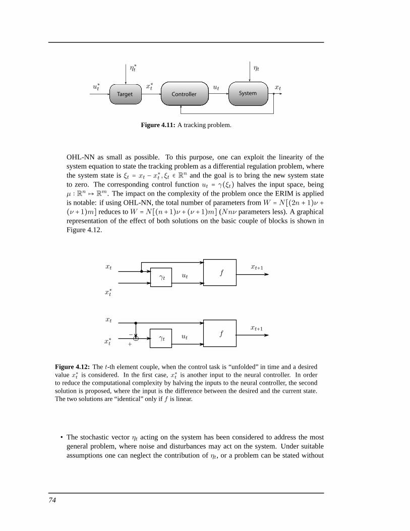
Target Controller Systemut xtx∗tu∗t
η∗t ηt
Figure 4.11: A tracking problem.
OHL-NN as small as possible. To this purpose, one can exploitthe linearity of thesystem equation to state the tracking problem as a differential regulation problem, wherethe system state isξt = xt − x
∗t , ξt ∈ Rn and the goal is to bring the new system state
to zero. The corresponding control functionut = γ(ξt) halves the input space, beingµ ∶ Rn
↦ Rm. The impact on the complexity of the problem once the ERIM is applied
is notable: if using OHL-NN, the total number of parameters fromW = N[(2n + 1)ν +(ν + 1)m] reduces toW = N[(n+ 1)ν + (ν + 1)m] (Nnν parameters less). A graphicalrepresentation of the effect of both solutions on the basic couple of blocks is shown inFigure 4.12.
−
+
xt
xt
xt+1
xt+1
x∗t
x∗t
ut
ut
γt
γt
f
f
Figure 4.12: The t-th element couple, when the control task is “unfolded” in time and a desiredvaluex∗t is considered. In the first case,x∗t is another input to the neural controller. In orderto reduce the computational complexity by halving the inputs to the neural controller, the secondsolution is proposed, where the input is the difference between the desired and the current state.The two solutions are “identical” only iff is linear.
• The stochastic vectorηt acting on the system has been considered to address the mostgeneral problem, where noise and disturbances may act on thesystem. Under suitableassumptions one can neglect the contribution ofηt, or a problem can be stated without
74

4. Optimal control by means of functional approximators
x0
u0γ0
x1
u1γ1
x2 // xN−1
uN−1γN−1
xNfff
Figure 4.13:Forward phase, when the system is (4.52).
anyηt since the beginning.8 In that case, the system equation is
xt+1 = ft(xt, ut), t = 0,1, . . . , T − 1 ; (4.52)
the control functionut = γt(xt) does not change, while the cost function does, accordingto the statement of the problem. If, for example,x0 is stochastic, then the cost functionto minimize is
F = Ex0
T−1∑t=0
ht(xt, γt(xt)) + hT (xT ) . (4.53)
A graphical representation of the chain of system and control blocks, unfolded in time,is shown in Figure 4.13.
4.3.3 A Receding Horizon technique
There are two main limitations to FH control. First, the horizonT must be known and fixeda priori, but often, feedback control systems must run for sufficiently long periods, and thecontrol horizon can be hardly “predicted”. This is the case of a robotic motion controller inparticular tasks, such as when a the target to reach is time-varying. In these ongoing processes,FH optimal control cannot be adopted: this issue is usually solved by seeking for Infinite Hori-zon (IH) controls (for example, optimal LQG regulators haveboth FH and IH formulations).
Second, variable or stochastic final states can be taken intoaccount if the ERIM is used,but in the general statement of aT -stage problem the final state is fixed, and the sequenceof optimal controls is open-loop. In other words, in Problem6 no changes are admitted,and if something in the problem statement changes, for example the target state, the con-trol sequence is no longer optimal. In addition, Receding Horizon (RH) control can be used[Kwon and Han, 2005]. The main advantage of RH control is thatit naturally yields closed-loop controls due to the repeated computation and implementation of only the first control ofan optimal sequence: this is substantially different from FH control, where the initial and finitestate to reach are fixed. The basic concept of RH is as follows.
At the current timet a sequence ofT optimal controls, minimizing aT -stage cost function,are derived, basically solving a FH problem like Problem 6. Precisely, the finite fixed horizontaken into account is[t, t + T ], and controls are denoted by
uFH0∣t , u
FH
1∣t , . . . , uFH
T−1∣t (4.54)
8Sometimes it is difficult to assess the effect of exogenous variables on the system, because these terms are notidentifiable or modeling is hard. Then either one includes inthe problem a generic random vectorηt or neglect thenoise.
75

where the suffixi∣t refers to thei-th control in the FH sequence generated at timet. Amongthe sequence of optimal controls computed on the fixed horizon [t, t + T ], only the first one isadopted as the current control law, hence
ut = uRH
t (xt) = uFH0∣t (4.55)
T defines the so called “Finite Horizon Sliding Window”. At staget+1, the same procedure isrepeated: the time interval[t+1, t+1+T ] is considered, and a sequence ofT optimal controlsis computed
uFH0∣t+1, u
FH
1∣t+1, . . . , uFH
T−1∣t+1
and then only the first is applied to the system. The procedureis repeated up to infinity, fort = t+2, t+3, . . ., where the corresponding time intervals are[t+2, T+2+T ], [t+3, T+3+T ], . . ..A graphical representation of the concept of RH is shown in Figure 4.15: notice that the term“receding” is indeed introduced since the horizon recedes as time proceeds. We point outthat the above receding horizon procedure implicitly defines a time-invariant control policyut ∶ Xt ↦ Ut of the formuRH
t (xt), as in Eq. 4.55, which is intrinsically closed-loop, as shownin Figure 4.14.
Target Controller System
FHOptimization
Solverxt
x∗t
x∗tuRHt
ηt
xt
J uFH0∣t , . . . , u
FH
T−1∣t
uFH0∣t
Figure 4.14:Using RH for closed loop control. The mechanism for selecting the first of a sequenceof FH optimal controls is reported with more clarity in Figure 4.15.
Stabilizing properties of RH control have been establishedfor different problem statements,for example under LQ assumptions [Kwon and Paearson, 1978, Kwon et al., 1983] and fornonlinear systems [Mayne and Michalska, 1990]. The solution was first provided using the ter-minal equality constraints,xt+T = 0, [Keerthi and Gilbert, 1988, Mayne and Michalska, 1990];such hard constraint was relaxed in [Michalska and Mayne, 1993], where the regulator wassimply required to drive the system to a neighborhood of the origin, where the control switched
76

4. Optimal control by means of functional approximators
uFH0∣t
uFH1∣t
uFHT−1∣t
uFH0∣t+1
uFH1∣t+1 uFH
T−1∣t+1
uFH0∣t+2
uFH1∣t+2
uFHT−1∣t+2
uRHt uRH
t+1
uRHt+2
t
t
t
t
Figure 4.15: The concept of a Receding Horizon controller. At time instant t = 0, the target valuex∗0
is measured, and a sequence of optimal controlsuFH
0∣0 , . . . , uFH
T−1∣0 is computed, consequently
with a FH trajectoryxFH
0∣0 , . . . , xFH
T−1∣0. Then only the first control is retained,u0= uFH
0∣0 . At timet = 1,2, . . ., the same procedure is repeated. Three consecutive “instants” are shown, forT = 4.
to a linear regulator designed to stabilize the nonlinear system, steering the state to its origin. In[Parisini and Zoppoli, 1995] the attractiveness of the origin was imposed by means of a penaltyfunction in the cost function.
A general RH control problem can be stated in the following way:
Problem 8. Given the fixed initial statex0 = x∗0 and a desired statex∗t
to reach, for the system:
xt+1 = ft (xt, ut, ηt) , t = 0,1, . . . ,∞wherext ∈ Xt ⊆ R
n, ηt is a stochastic variable with known distribution; find the optimalcontrols ut ∈ Ut whereut is the first of a sequence ofT optimal controlsu
0∣t, . . . , uT−1∣t,
having the form
u0∣t = γ0(xt) ∈ Ut(xt) ⊆ Rm
77

which minimize at each time instantt the cost functional
F = Eη0∣t,...,ηT−1∣t
J = Eη0∣t,...,ηT−1∣t
T−1∑i=0
hi(xi∣t, γi (xi∣t)) + hT (xT ∣t) (4.56)
wherex∗0∣t = xt andx∗
T ∣t = x∗t .
Notice that the control functionsγi, i = 0, . . . , T − 1 are time-invariant, i.e.γi∣t = γi,∀t. Aspreviously pointed out for Problem 6, in (4.56) there is not an explicit reference of the desiredstate in the cost functionJ . It is straightforward to notice the relationship between Problem 6and Problem 8: the RH controlut is the first of the optimal controls which are effectivelycomputed once a specific instance of Problem 6, where the initial statex∗0 of the FH problem isthe current statext in the RH problem (x∗
0∣t = xt) while the desired statex∗T is set to the sameof the RH problem (x∗
T ∣t = x∗t ).Incidentally, one may notice that if both initial and desired state to reachx∗
tare known
a priori, exploiting the reachability properties one may think of directly implementing a FHcontrol. However, due to the stochastic noise, the reachability in T stages may not be satisfiedor guaranteed, thus a RH control law would be more indicated.
However, the main motivation for using a RH controller is that it can easily deal with atime-varyingx∗t to reach. In particular, in this case a certain principle must be assumed.
Certainty Equivalence
Whenever the controlled system has to track a desired target, or its decisions depend upon theevolution of a certain system, the RH can be easily applied ifcombined with the so calledCertainty EquivalencePrinciple (CE/CEP).
The CE is fundamental when the target is time-varying,x∗t , and its dynamics and statisticalproperties are unknown or unpredictable, but it is perfectly measurable at time instantt. Inthis case, everyt the RH controller is designed as if the stochastic quantityx∗t would remainunchanged in the future, fort, t + 1, . . . ,∞. For example, if the target at instantt is in the statex∗t, the controller would assumex∗t = x∗t ,∀t > t. At time t+1, a new measurex∗
t+1 of the targetis provided, so the controller would assumex∗t = x∗t+1,∀t > t + 1. The procedure is repeatediteratively. The corresponding RH control problem is:
Problem 9. Given the fixed initial statex0 = x∗0 and a time-varying desired statex∗t to reach,for the system:
xt+1 = ft (xt, ut, ηt) , t = 0,1, . . . , t <∞wherext ∈ Xt ⊆ R
n, ηt is a stochastic variable with known distribution; find the optimalcontrolsut ∈ Ut ⊆ Rm whereut is the first of a sequence ofT optimal controlsu
0∣t, . . . , uT−1∣t,
having the formui∣t = γi (xt) ∈ Ut(xt) ⊆ Rm , i = 0, . . . , T − 1
which minimize at each time instantt the cost functional
F = Eη0∣t,...,ηT−1∣t
J = Eη0∣t,...,ηT−1∣t
T−1∑i=0
hi(xi∣t, γi(xi∣t)) + hT (xT ∣t)
78

4. Optimal control by means of functional approximators
wherex∗0∣t = xt andx∗
T ∣t = x∗t .
0 1 2 4 53 6 7 8
x∗t xt
xFHi∣0
x
t
Figure 4.16: An example of tracking when a RH controller is used. A time-varying targetx∗
is tracked by a system, where a RH controller is used to find theoptimal controlsu and thecorresponding “optimal” state trajectoryx. At each time instant, the CEP is applied, and aT
stages - FH problem is solved. Here, the finite horizon isT = 6. At time instantt = 0, the targetvaluex∗0 is measured, a sequence of optimal controlsuFH
0∣0 , . . . , uFH
5∣0 is computed, consequently
with a FH trajectoryxFH
0∣0 , . . . , xFH
5∣0 . Then only the first control is retained,u0= uFH
0∣0 , and the
system statex1= xFH
1∣0 is found. The procedure is repeated iteratively fort = 1,2, . . .. In figure, the
FH trajectoriesxFH
i∣t , i = 0, . . . ,5, ∀t are shown, as well as the final RH trajectoryxt .
We remark that in Problem 9 there are no assumptions or modelsof the target behavior.This means that the RH controlsut are “locally” optimal, with respect to the current measureof the target. Combining the RH framework with the CEP, meansthat at each staget, theToptimal controls are derived, with the stochastic quantityremaining constant: that is, in thecase of tracking, considering the target trajectory to hold, as shown in Figure 4.16.
It is now evident that the main advantage of RH control is thatit yields closed-loop controlswhich can counteract to disturbances and time-varying parameters, due to the repeated com-putation and implementation of only the first control of a sequence which is “optimal” giventhe current problem statement: so at each time instantt, the initial and desired state of a newinstance of FH problem are set, after measuring the current system and target state. This issubstantially different from FH control, where the initialand finite state to reach are fixedapriori . In particular, as already observed for Problem 6, variableor stochastic final states canbe taken into account if the ERIM is used, but in the general statement of aT -stage problemthe final state is fixed, and the sequence of optimal controls is computed in “open-loop” (and isa sequence of numerical values, not functions).
79
ERIM and RH control
The classical RH technique assumes that a FH optimization routine computes at each con-trol instantt a sequence of optimal controls: basically the control vectors are generated afterthe solution of a nonlinear programming problem at each timeinstantt. This procedure canbe implemented in real applications only if the process dynamics is sufficiently “slow”, i.e.the time between two consequent controls is enough to solve aFH control problem. This as-sumption is unrealistic in the case of humanoid robotics, asthe robot (and sometimes alsothe target) dynamics is fast and the complexity of the problem generally increases with thenumber of DOF to control. In order to solve the optimization problem on-line, with the guar-antee of satisfying the temporal constraint, a proper hardware and software are required: atleast, one should be provided with a real-time processing unit supporting fast and highly pre-cise computations, directly connected to the robot sensingand actuation devices (to avoid de-lays). Unfortunately, different multi-level control architectures often do not support this controlscheme. Both iCub and James, for example, cannot support it,as shown in Figure 4.14, be-cause the PC104 “controlling” the robot is not more than an interface to the cluster (wheredemanding computations are performed), and cannot bear such computations. This fact moti-vates the use of the ERIM in this problem: since it allows concentrating in an off-line phaseall the computational burden required to approximate the optimal control functions, in the on-line phase the control actions can be promptly generated with a small computational effort[Ivaldi et al., 2008a, Ivaldi et al., 2008b].
Remark 11. The ERIM can be generalized also for Infinite Horizon (IH) control. In practi-cal applications, the impossibility of applying the ERIM tothe IH case is basically due to thenecessity of using a chain containing an infinite number of neural networks, which leads to acontroversy in the initialization of the backward phase when finding the optimal parameters ofthe functional approximators [Pianosi and Soncini-Sessa,2008]. A workaround is to approx-imate and “truncate” the cost, for example assuming that at staget the IH for the backwardphase “starts” at t, wheret ≪ t < t∞. However, the complexity of the solution in this case isconsiderably high, and justified only for offline precomputation of the optimal control laws, orin applications where the dynamics of the controlled systemis particularly “slow”, such as inmanagement of water reservoirs [Pianosi, 2008].
Applying the ERIM to a RH control problem is very easy. Following the same proceduredescribed for turning Problem 6 into Problem 7, applying theERIM consists in constraining thefinite sequence of control functions, generated at each timeinstantt, to take on a fixed structurewith a certain number of parameters to be optimized. More precisely, Problem 9 becomes:
Problem 10. Given the fixed initial statex0 = x∗0 and a time-varying desired statex∗t to reach,for the system:
xt+1 = ft (xt, ut, ηt) , t = 0,1, . . . ,∞wherext ∈ Xt ⊆ R
n, ηt is a stochastic variable with known distribution; find the vectorsof optimal parameterswt ,∀t corresponding to the optimal controlsut ∈ Ut ⊆ R
m with thefollowing structure:
ut = γ(xt,w)
80
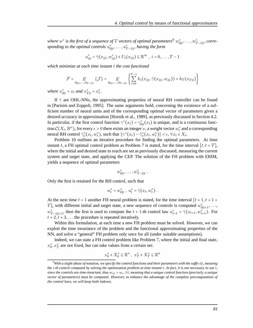
4. Optimal control by means of functional approximators
wherew is the first of a sequence ofT vectors of optimal parameters9 w0∣t, . . . ,w
T−1∣t, corre-
sponding to the optimal controlsu0∣t, . . . , u
T−1∣t, having the form
ui∣t = γ(xi∣t,wi∣t) ∈ Ut(xi∣t) ⊆ Rm , i = 0, . . . , T − 1which minimize at each time instantt the cost functional
F = Eη0∣t,...,ηT−1∣t
J = Eη0∣t,...,ηT−1∣t
T−1∑i=0
hi(xi∣t, γ(xi∣t,wi∣t)) + hT (xT ∣t)wherex∗
0∣t = xt andx∗T ∣t = x∗t .
If γ are OHL-NNs, the approximating properties of neural RH controller can be foundin [Parisini and Zoppoli, 1995]. The same arguments hold, concerning the existence of a suf-ficient number of neural units and of the corresponding optimal vector of parameters given adesired accuracy in approximation [Hornik et al., 1989], aspreviously discussed in Section 4.2.In particular, if the first control functionγ(xt) = γ0∣t(xt) is unique, and is a continuous func-tionC(Xt,R
n), for everyε > 0 there exists an integerν, a weight vectorwt and a correspondingneural RH controlγν(xt,wt ), such that∥γ(xt) − γν(xt,wt )∥ < ε, ∀xt ∈Xt.
Problem 10 outlines an iterative procedure for finding the optimal parameters. At timeinstantt, a FH optimal control problem as Problem 7 is stated, for the time interval[t, t + T ],where the initial and desired state to reach are set as previously discussed, measuring the currentsystem and target state, and applying the CEP. The solution of the FH problem with ERIM,yields a sequence of optimal parameters
w0∣t, . . . ,w
T−1∣t .
Only the first is retained for the RH control, such that
wt = w0∣t , ut = γ(xt,wt ) .At the next timet + 1 another FH neural problem is stated, for the time interval[t + 1, t + 1 +T ], with different initial and target state, a new sequence of controls is computedw
0∣t+1, . . .,wT−1∣t+1, then the first is used to compute thet + 1-th control lawut+1 = γ(xt+1,wt+1). For
t + 2, t + 3, . . . the procedure is repeated iteratively.Within this formulation, at each time a new FH problem must besolved. However, we can
exploit the time invariance of the problem and the functional approximating properties of theNN, and solve a “general” FH problem only once for all (under suitable assumptions).
Indeed, we can state a FH control problem like Problem 7, where the initial and final state,x∗0 , x
∗T are not fixed, but can take values from a certain set:
x∗0 ∈ X∗0 ⊆ Rn , x∗T ∈ X∗T ⊆ Rn
9With a slight abuse of notation, we specify the control functions and their parameters with the suffixi∣t, meaningthei-th control computed by solving the optimization problem attime instantt. In fact, it is not necessary to uset,since the controls are time-invariant, thuswi∣t = wi,∀t, meaning that a unique control function (precisely, a uniquevector of parameters) must be computed. However, to enhancethe advantage of the complete precomputation ofthe control laws, we will keep both indexes.
81

in that case, the cost functional must include them in the expectation ofJ , i.e.
F = Ex∗0,x∗
T,η0,...,ηT−1
J
and the same for the control laws, whose outputs necessarilydepend on the boundary values,in the most general form:ut = γ(xt, x∗0 , x∗T ,w),∀xt ∈ Xt ⊆ R
n, where the approximatedoptimal controls are generated for any possible instance ofa FH control problem, given theknown stochastic boundary conditions. In that case, Problem 10 becomes:
Problem 11. Given the fixed initial statex0 = x∗0 and a time-varying desired statex∗t to reach,for the system:
xt+1 = ft (xt, ut, ηt) , t = 0,1, . . . ,∞wherext ∈ Xt ⊆ R
n, ηt is a stochastic variable with known distribution; find the vector ofoptimal parametersw corresponding to the optimal controlsut ∈ Ut ⊆ Rm with the followingstructure:
ut = γ(xt, x∗t ,w)wherew is the first of a sequence ofT vectors of optimal parametersw0, . . . ,wT−1, corre-sponding to the optimal control functions having the form
ui = γi (xi, x∗0 , x∗T ,wi) ∈ Ui(xi) ⊆ Rm , i = 0, . . . , T − 1wherex∗0 = xt, x∗T = x∗t , which minimize at each time instantt the cost functional
F = Ex∗0,x∗
T,η0,...,ηT−1
J = Ex∗0,x∗
T,η0,...,ηT−1
T−1∑i=0
hi(xi, γ(xi,wi)) + hT (xT )
wherex∗0∈ X∗
0⊆ Rn andx∗T ∈ X∗T ⊆ Rn.
The fundamental difference between Problem 10 and Problem 11 is that while the firstrequires the execution of the optimization procedure at each time instantt (i.e. the solutionof a specific FH problem), the latter requires the solution ofa more generalized (yet morecomplex) FH control problem only once. The main advantage ofthis approach, is that it ispossible to pre-compute explicitly, upon a desired approximation accuracy, the optimal RHcontrol law, completely in an off-line phase. The information of the optimal RH control lawlies on the vector of optimal parameters,w, that is on a finite number of real values. Thus, oncethe control law is computed, it can be easily implemented andembedded in real-time controlloops: at any time instantt, given the target and system measurementsx∗t , xt, the computationof the associated optimal controlu is almost instantaneous, being a simple forward of a NN (afinite number of sums and products). A scheme illustrating the benefits of this solution whenapplied to closed loop control is shown in Figure 4.17.
The pseudo-code for the solution of Problem 11 is shown in Algorithm 2.
82

4. Optimal control by means of functional approximators
Algorithm 2 Receding-Horizon procedure combined with ERIM, for the solution of Prob-lem 11.
“Online” RHEnsure: ut , ∀t
1: Pre-computew = Offline FH(T,X∗0,X∗T )
2: loop3: Measurex∗t , xt4: Apply ut = γ(xt, x∗t ,w)5: end loop
“Offline” FHRequire: T ,X∗0 ,X∗TEnsure: w = w0, . . . ,wT−1
1: k = 02: Initialize w(k) randomly or according to some specific technique3: repeat4: Generateη0(k), . . . , ηT−1(k) according to their probability density5: Generatex∗
0(k), x∗T (k) according to their distribution overX∗
0,X∗T
6: Initialize x0(k) = x∗0(k)Forward
7: for t = 0 ∶ T − 1 do8: Computeut(k) = γ(xt(k), x∗T ,wt(k))9: Computext+1(k) = ft(xt(k), ut(k), ηt(k))
10: Compute∂ht
∂xt(k) ,∂ht
∂ut(k) ,∂ft
∂xt(k) ,∂ft
∂ut(k)11: end for
Backward
12: Compute∂J
∂xT (k)13: for t = T − 1 ∶ 0 do
14: Compute∂J
∂ut(k)15: Compute
∂J∂xt(k)
16: for i = 0 ∶Wt do
17: Compute∂J
∂wit(k)
18: Update weightwit(k)
19: end for20: end for21: until Convergence condition is met22: return w = w(k)
83
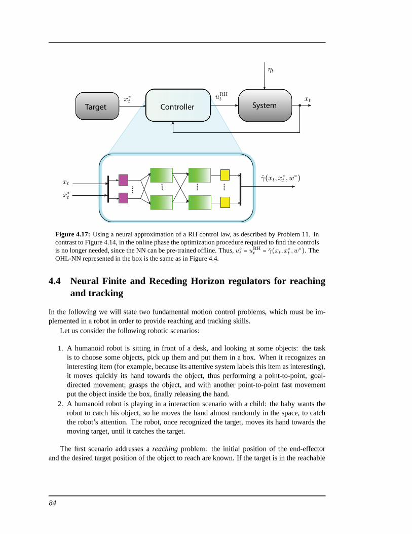
Target Controller System
xt
x∗t
x∗tuRHt
ηt
xt
γ(xt, x∗t ,w)
Figure 4.17: Using a neural approximation of a RH control law, as described by Problem 11. Incontrast to Figure 4.14, in the online phase the optimization procedure required to find the controlsis no longer needed, since the NN can be pre-trained offline. Thus,ut = uRH
t = γ(xt, x∗t ,w
). TheOHL-NN represented in the box is the same as in Figure 4.4.
4.4 Neural Finite and Receding Horizon regulators for reachingand tracking
In the following we will state two fundamental motion control problems, which must be im-plemented in a robot in order to provide reaching and tracking skills.
Let us consider the following robotic scenarios:
1. A humanoid robot is sitting in front of a desk, and looking at some objects: the taskis to choose some objects, pick up them and put them in a box. When it recognizes aninteresting item (for example, because its attentive system labels this item as interesting),it moves quickly its hand towards the object, thus performing a point-to-point, goal-directed movement; grasps the object, and with another point-to-point fast movementput the object inside the box, finally releasing the hand.
2. A humanoid robot is playing in a interaction scenario witha child: the baby wants therobot to catch his object, so he moves the hand almost randomly in the space, to catchthe robot’s attention. The robot, once recognized the target, moves its hand towards themoving target, until it catches the target.
The first scenario addresses areachingproblem: the initial position of the end-effectorand the desired target position of the object to reach are known. If the target is in the reachable
84

4. Optimal control by means of functional approximators
space of the robot’s workspace, and a certain movement duration can be estimated, it is possibleto state the reaching problem as a FH optimal control problem.
The second scenario addresses instead atracking problem: the initial position of the end-effector is known, however the target position is known onlyinstantly (at each measurement),since it changes rather unpredictably (although smoothly). Moreover, it is hard to cast a pre-diction on the movement duration: in this case, it is possible to state the tracking problem asan IH or RH optimal control problem.
In the previous Sections, it was shown how the ERIM can approximate numerically theoptimal solution to such problems. Another advantage of this approach, is that once the struc-ture of the control functions is fixed (i.e. OHL-NN withν “neurons”), it is possible to switchfrom one solution to the other by simply loading a new set of parameters, which is merely avector of real numbers. Thus, one can build a “neutral” NN control function on the main boardconnected to the robot (i.e. the PC104 for iCub), and then simply load the right set of parame-ters for any desired control task. Furthermore, not only it is possible to switch from FH to RHcontrollers, but also among different FH controllers, where the cost function to minimizeJ hasbeen chosen to implement different computational motor control models, as the ones describedin Chapter 3. That is one can switch from reaching with the MJM(Section 3.2.1), to reach-ing with the MTCM (Section 3.2.2), to tracking minimizing a simple quadratic cost function.Switching can be done online, because the optimal control functions are pre-computed in an of-fline phase, where the NNs are “trained” with iterative procedures like the ones in Algorithm 1and Algorithm 2.
Let us now state the problems more specifically.Let us denote byxr the Cartesian coordinates of the end-effector of the robot,with respect
to a fixed reference frame, byq, τ the corresponding vectors of the manipulator joints coordi-nates and torques, respectively. Then the forward kinematics isxr = farm(q) ∶ Rnq ↦ R
nx ,and can be easily retrieved by means of the Denavit-Hartenberg description of the robot kine-matics [Sciavicco and Siciliano, 2005]. The forward dynamics can be instead described by therigid-body dynamics model. We remark that:
• q ∈ Rnq is the vector of joints coordinates, and can be different (conceptually) from thevector of controlled joints;
• xr ∈ Rnx is usually a vector withdim(xr) = 3,6,7 depending on what is controlledamong the Cartesian coordinates: position only, or position and orientation
The generic Cartesian coordinates of the target are denotedby xg ∈ Rnx. At time instantt, therobot and target state vectors arexrt , x
gt .
It is assumed that the following compact model can be used to describe the evolution of theend-effector with respect to the target, if the controlut acts on the robot:
ξt+1 = f (ξt, ut) , t = 0,1, . . . (4.57)
where at time instantt, ξt is the big state vector, taking values from a finite setΞ ⊆ Rn, andutis the control vector, constrained to take values from a finite setU ⊆ Rm.
85

γt γt+1
xgt x
gt+1
xrt xrt+1ut ut+1
TT
RR
Figure 4.18: A conceptual scheme, representing the interaction among robot, target, and neuralcontrols, unfolded in time.T accounts for the “target”, whileR for the “robot”. γt can be either aFH control law,γ(⋅,wt ), wherewt = wFH
t , or a RH control lawγ(⋅,w), wherew = wRH.
Remark 12. Here, we keep the problems statement as generic as possible:indeed, we donot specify neither the nature ofut nor the one ofξt. For example, the control vectorutcan be a velocity joint command, or a joint torque command;ξt can be generically a vectordescribing the difference between the current end-effector coordinates and the target ones,ξt ≜ [xgt − xrt ], or a more detailed vector containing position, velocities, acceleration errors,etc. (e.g.ξt ≜ [xgt −xrt , xgt − xrt ]). Consequently, we do not specify the structure off , that couldbe a pure kinematics or dynamics model, or a combination of both.
Assumption 11. The robot kinematics and dynamics model is perfectly known.
Thanks to Assumption 11, it is possible to write Eq. 4.57, where f is perfectly known.Moreover, thanks to the time invariance of the systemf (and of the cost function),t = 0 canbe considered as a generic time instant. The goal of the reaching control problem is to find,at time instantt, a sequence ofN optimal controlsu
0, . . . , uN−1 that minimize a suitable cost
functionJ , which is chosen so as to characterize the trajectory of the system stateξi, which issteered from an initial stateξ0 towards a desiredξ∗.J takes generally the following form
J = N−1∑i=0
hi(ξi, ξ∗, ui) + hN(ξN) (4.58)
wherehN , hi are partial cost terms. A typical cost structure in automatic controls is:
J = N−1∑i=0
Pi ∥ui∥2 + Vi ∥ξi∥2 + VN ∥ξN∥2 (4.59)
wherePi, Vi, VN are suitable positive definite weight matrices. Ifξi ≜ xg(t) − xr(t) then(4.59) penalizes generically the error between the Cartesian coordinates of end-effector and ofthe target to reach, at the end and during the whole trajectory (seeVN andVi), along with apenalty on the amount of “energy” spent for the controls. Some examples of cost functions forcomputational motor control models have been presented in Chapter 3.
Then, the neural reaching problem can be stated as follows, as a FH optimization problem:
Problem 12 (Neural Reaching). Given the system of Eq. 4.57, find the vectors of optimalparametersw0, . . . ,w
N−1 that minimize the cost function
F = Eξ0∈Ξ,ξ∗∈Ξ∗
N−1∑i=0
hi(ξi, ξ∗, γ(ξi, ξ∗,wi)) + hN(ξN , ξ∗)
86

4. Optimal control by means of functional approximators
under the constraints given by the state equation, where controls take on the structureui =γ(ξi, ξ∗,wi) ∈ U ⊆ Rm.
It is remarked that the problem is generalized for any possible initial stateξ0 ∈ Ξ and desiredstateξ∗ ∈ Ξ∗ (i.e. for every possible robot and target’s coordinates), in virtue of the expectationoperatorE. The solution of Problem 12 follows the aforementioned iterative procedure for thesolution ofT -stage FH problems. It is important to point out that once theproblem is solved,the set of vectorsw0, . . . ,w
N−1 explicitly carry the information about the optimal controllaws.
Incidentally, the solution of Problem 12 allow solving without effort the correspondingRH problem. Indeed, by making the assumption that at time instant t the target stateξ∗t = 0
will hold for N stages, thus applying a CEP, it is possible to exploit the first FH control lawand apply it as a RH control law, as previously discussed. This method particularly fits tothe tracking unknown/unpredictable targets: the robot assumes the target to retain the currentposition whenever a new measurement is available, and movestoward it as if the plannedtrajectory would assume it fixed forN stages. A change in the target’s position does not affectthe tracking policy, since at each time instant the target’scoordinates are measured and theproper control corresponding to a newer trajectory is performed.
Then, the neural tracking problem can be stated as follows, as a RH optimization problem:
Problem 13 (Neural Tracking). Given the system of Eq. 4.57, find the vector of optimal para-metersw, being the first among the setw0, . . . ,w
N−1 that minimize the cost function
F = Eξ0∈Ξ,ξ∗∈Ξ∗
N−1∑i=0
hi(ξi, ξ∗, γ(ξi, ξ∗,wi)) + hN(ξN , ξ∗)under the constraints given by the state equation, where controls take on the structureui =γ(ξi, ξ∗,wi) ∈ U ⊆ Rm.
Oncew = w0 is found, the generic tracking control law is:
ut = γ(ξt, ξ∗t ,w)that is a generic, time-invariant closed loop control function.
Since the RH problem exploits the solution of the corresponding FH problem, only thelatter must be solved. The solution of the aforementioned problems is based on the forward-backward algorithm: Figure 4.18 shows a simple scheme with the “chain” of NN, target andsystem blocks, unfolded in time, which are used for computing the optimal parameters (seealso [Ivaldi et al., 2010]).
4.5 Numerical results
In the following, we will discuss some numerical results, where two peculiar systems havebeen tested in a variety of problems settings, both in reaching and tracking mode: a 2DOFrobotic manipulator and a 3DOF nonholonomic mobile robot. The aim was to analyze theperformances of the proposed methods on relatively simple nonlinear systems with respect to
87

the growing complexity of the problem. In particular, the idea to use a simple nonlinear systemwas inspired by the desire to apply the method directly at joint level control, thus combiningthe optimal planning with the low-level task to joint space conversion modules.
Numerical simulations show interesting results: however,even if the proposed methodsshow some evident advantages, there are many practical issues which have to be taken intoaccount, and which we believe could set limitations on the application domain of the methods.First, the method can manage only theoretically a significant number of parameters withoutincurring in the COD, i.e. the exponential growth of the number of parameters with the com-plexity of the problem, because their growth is actually polynomial [Zoppoli et al., 2001]. Butthe number of parameters is still very high, due to the fact that the number of controlsN mustbe large enough to provide a plausible sequence of controls,and similarly each NN can pro-vide sufficient approximation capability for wide class of functions only with large number ofparameters. The second issue is the training complexity, which is a combination of the effectsof the number of parameters, the back-propagation algorithm, and the stochastic gradient. Thethird issue is related to the stochastic formulation and theconsequent amount of training data,and the time required to train the chain. Finally, the initialization of the OHL-NN can play arole, as a randomized initialization is correct from a theoretical point of view, and is the onlyplausible way to initialize the neural network if there is noa priori hypotheses on the structureof the control laws. If any information on their “shape” is available, it could be useful to ini-tialize the networks differently, for example with a classical least-squares algorithm. A moredetailed analysis of these defects is reported in Section 4.5.4.
4.5.1 A two DOF manipulator in a planar space
In the following preliminary numerical results concerningthe control of an anthropomorphicarm are presented. For the sake of simplicity, a two DOF arm isused: the main reason is thepossibility to easily compute both Cartesian and joint coordinates easily, as the forward andinverse kinematics are known, and asn =m = 2 the manipulator is not redundant. The forwardkinematics of the planar arm is:
xr = l1 cos q1 + l2 cos(q1 + q2)yr = l1 sin q1 + l2 sin(q1 + q2) .
whereq1, q2 are the joints angles, whilexr, yr the Cartesian coordinates of the end-effector intheX − Y planar space. A representation is shown in Figure 4.19.
Point-to-point movement with the MJM
With the following numerical example, we want to verify the capability of a chain of neuralnetworks to approximate a desired control function minimizing a certain cost, upon a desiredaccuracy. Here, the “neural controllers” must drive the end-effector from an initial to a desiredposition in the robot’s workspace, with initial and final null velocities.
The “neural controllers” must drive the end-effector of a manipulator from any initial po-sition ξ0 = [x0, y0] ∈ X ⊆ R2 to a final desiredξ∗ = [x∗, y∗] ∈ X ⊆ R2. The initial and final
88

4. Optimal control by means of functional approximators
Y
Xq1
q2
l1
l2
(xr, yr)
Figure 4.19:A simple model of a two DOF planar arm.
velocity must be equal to zero. The MJM has been chosen as a computational model describingthe motion trajectory, and the followingminimum jerkis the cost criterion:
J = ∫ T
0
⎡⎢⎢⎢⎢⎣(d3xrdt3)2 + (d3yr
dt3)2⎤⎥⎥⎥⎥⎦dt (4.60)
As shown in Figure 4.20, the MJM produces bell-shaped, smooth trajectories in the joint space,while the planar trajectory is almost straight. The known analytical solution has been comparedwith the “neural” trajectory: withN = 60, OHL-NN with sigmoidal activation function andlinear output layer, andν = 40, the accuracy in the approximation was very high.
Tracking a point moving unpredictably
An instance of Problem 13 has been stated with the following cost function:
J = N−1∑i=0
c(ui) + ξTi+1Vi+1ξi+1 (4.61)
whereξi = [xri − xgi , yri − ygi ] ∈ X ⊆ R2, ξ∗ = 0, N = 30, ν = 40, OHL-NNs with sigmoidal
activation function. f was basically a double integrator. Approximately109 samples wereused for the off-line training of the NNs, considering any possible position of both target andend-effector in the reachable space. The criterion for the task accomplishment in (4.61) isa tradeoff between the minimization of the energy consumption and the “best” end-effectorproximity to the target during and at the end of the maneuver (it could not be able to reach itperfectly, as a consequence of the unpredictable behavior of the target or the robot’s intrinsicphysical limits). Weight matricesVi were chosen such as to obtain a reasonable compromisebetween the attractiveness of the target and the energy consumption, whereasc(uj,t), j = x, yis a nonlinear but convex function [Ivaldi et al., 2008c]:
c(uj,t) = α [ 1βln(2 + eβuj,t + e−βuj,t) − 1
βln(4)] , j = x, y (4.62)
which, for large values ofβ approximates the ideal but non differentiable costα ∣uj,t∣, as shownin Figure 4.22. Of course,uj,t indicates thej-th component of the control at time instantt, i.e.
89

0.4 0.35 0.3 0.25 0.2 0.15 0.1 0.05 0−0.05
0
0.05
0.1
0.15
0.2
0.25
0.3
0.35
x [m]
y [m]
t=0
t=N
0 60300
0.1
0.2
0.3
0.4Cartesian position of the end−effector
time instants
[m]
0 30 60−1
−0.5
0
0.5Cartesian velocity of the end−effector
time instants
[m/s
]
0 30 60−0.5
0
0.5
1
1.5
2Arm joints angle position
time instants
[rad
]
0 6030−2
0
2
4Arm joints angular velocity
time instants
[rad
/s]
xy q
1
q2
xy
q1
q2
Figure 4.20: A minimum jerk planar movement of a two DOF arm: Cartesian andjoints positionand velocity are shown, as well as samples of the planar trajectory. The neural approximation andthe analytical solution [Flash and Hogan, 1985] are almost coincident (MSE≅ 10−7).
90

4. Optimal control by means of functional approximators
0.25 0.2 0.15 0.1 0.05 0
0
0.05
0.1
0.15
0.2
0.25
x [m]
Robot trajectory in the x−y plane.
y [m]
end-e!ector
target
(t=0)
t=N
(t=0)
0 20 40 600
0.05
0.1
0.15
0.2
0.25Cartesian position of the end−effector
time instants
[m]
xy
0 20 40 60−0.04
−0.02
0
0.02
0.04Cartesian velocity of the end−effector
time instants
[m/s
]
xy
0 20 40 600
0.5
1
1.5
2
2.5Arm joints angle position
time instants
[rad
]
q1
q2
0 20 40 60−0.15
−0.1
−0.05
0
0.05Arm joints angular velocity
time instants
[rad
/s]
q1
q2
Figure 4.21:The end-effector of a two DOF arm, tracking a point moving in an unpredictable wayon a planar space.
91

ut. Moreover,Vi = diag(1.0,80.0,5.0, 10.0), i = 0, . . . ,N − 1, VN = 40I (beingI the identityor unit matrix), whileα = 0.01 andβ = 50. In Figure 4.21 the end-effector, starting still ina certain position, tracks a target moving unpredictably inthe space. Cartesian coordinates aswell as joints coordinates (for the two DOF) during the movement are shown. It is worth notingthat although the target dynamics is quite fast, and the end-effector was initially “far” from thetarget, the arm follows the moving point with reasonable performances.
−5 −4 −3 −2 −1 0 1 2 3 4 50
1
2
3
4
5
c(uj i)
uji
Figure 4.22: The cost function (4.62), withK = 0.01 andβ = 50.
F
x
y
Tθ
u1
u2
d
Figure 4.23:The mobile robot described by Eq. 4.63.
4.5.2 A three DOF nonholonomic mobile robot in a planar space
A nonholonomic mobile robot moves on a planar space. The robot position with respect to thecoordinate system is described by the Cartesian coordinates in the spacex,y and by the angleθ of its axis of symmetry with respect to thex axis (see Figure 4.5.1). On the robot sides twocouples of thrusters, aligned with the axis of symmetry, aremounted at constant distanced,and can be modulated so as to obtain the desired intensity of the forceF and the desired torque
92

4. Optimal control by means of functional approximators
C by which to control the robot motion. The thrusts identify the two controlsu1 andu2:
F = (u1 + u2)e =mx
C = (u1 − u2)d = Jθ (4.63)
Massm and moment of inertiaJ are assumed to be constant during the maneuver. The systemstateξ is then composed of six variables,ξ = col(x, x, y, y, θ, θ), and the nonlinear differentialdynamic of the robot is:
ξ1 = ξ2, ξ3 = x4, ξ5 = ξ6 ,ξ2 = 1
m(u1 + u2) cos ξ5 , ξ4 = 1
m(u1 + u2) sin ξ5 , ξ6 = d
J(u1 − u2)
subject to constraints to the maximum allowed thrust values: ∣ui∣ ≤ U, i = 1,2.Let us now denoteξt ≜ ξ(t∆t), ut ≜ u(t∆t), where∆t is the sampling period, obtained
by dividing the durationT of the maneuver intoN discrete stages. As done before, thej-thcomponent of vectorsξt, ut is denoted byξj,t, uj,t. Then a discrete-time version of the systemcan be obtained by using a first-order Euler’s approximation:
ξ1,t+1 =ξ1,t +∆t ξ2,t
ξ2,t+1 =ξ2,t +∆t1
m(u1,t + u2,t) cos(ξ5,t)
ξ3,t+1 =ξ3,t +∆t ξ4,t
ξ4,t+1 =ξ4,t +∆t1
m(u1,t + u2,t) sin(ξ5,t)
ξ5,t+1 =ξ5,t +∆t ξ6,t
ξ6,t+1 =ξ6,t +∆td
J(u1,t − u2,t)
which can be written in a more general and compact form as
ξt+1 = f(ξt, ut) , t = 0,1, . . . ,N − 1whereξt may take values from a finite setXt ⊆ R
n, while ut is constrained to take valuesfrom a finite setUt(ξt) ⊆ Rm (related to the physical limits of the thrusters). The desired robotconfiguration at instantt is denoted byξ∗t : a desired trajectory to track can be described by thesequence of vectorsξ∗
0, . . . , ξ∗N .
It is important to remark that the linearized models of such nonholonomic systems are notcontrollable. So far a number of control strategies have been proposed. In [Aicardi et al., 1995]a Lyapunov stabilizing control law was proposed, while in [Gu and Hu, 2005] a switching con-troller was presented, based on a Lyapunov-like function, gathering stability over a recedinghorizon. In [Parisini and Zoppoli, 1995] a receding horizoncontrol strategy was introduced,which was based on the use of neural approximators: in particular, the generalized control lawwas found as the best interpolation of a set of optimal deterministic controls, within a specifictraining set.
93

A reaching problem over a Finite Horizon
We address the problem of regulating the planar robot in Figure 4.5.1, that is to steer the robottowards a target positionξ∗ from any initial one, by minimizing a certain cost function,whichgenerally takes into account the fuel consumption and the maneuver accuracy. The criterion forthe task accomplishment is a tradeoff between the minimization of the fuel consumption, takeninto account by a general nonlinear convex functionc(ui,t), (i = 1,2), and the “best” robotproximity to the target at the end of the maneuver ( it could not be able to reach it perfectly, asa consequence of the robot’s intrinsic physical limits):
J = N−1∑t=0
c(u1,t) + c(u2,t) + ∥ξ∗t+1 − ξt+1∥2Vt+1(4.64)
As previously done for the manipulator example, the weight matricesVt are chosen so as toobtain a reasonable compromise between the attractivenessof the target and the fuel consump-tion. More specifically, we usedN = 10 control stages inT = 10 (so∆t = 1.0); moreoverVt = diag[1,0.1,40.0,0.1, 40.0,0.1], for t = 1, . . . , T − 1, andVN = diag(40.0). c(ui,t) hasbeen indeed designed to be realistically proportional to the thrust, and approximate at the sametime the ideal but non differentiable costK ∣ui,t∣: again, we used Eq. 4.62, withK = 0.01 andβ = 50. The control functions were implemented by OHL-NN, using12 inputs variables (6from ξt and6 from ξ∗t ) andν = 80 neural units in the hidden layer.
A tracking problem over a Receding Horizon
There are many applications of mobile robots following a target: for example, when they mustfollow a human as their leader. To this purpose, a RH regulation problem can be stated. As donefor the 2 DOF, an instance of Problem 13 has been stated. Again, the general RH control lawcan be easily found after the solution of the equivalent FH regulation problem, which is statedfor any possible robot and target configuration. In detail, aset ofL admissible configurationsof both robot and target,xr andxg were generated, then fed to the iterative algorithm for thecomputation of the optimal parameters of the approximatingNNs. Note that formulating theproblem as a regulation one, the system state (i.e. the difference between robot and target) issteered to the origin of the state space: this brings the advantage to halve the number of inputsto the NN, as already discussed in Figure 4.12. In the following numerical examples, the costis the same as in (4.64),N = 30, ∆t = 1s and the OHL-NNs haveν = 80 neurons.
Figure 4.25 shows some FH trajectories, after≈ 106 training steps, which have been usedto provide the solution to the RH problem. It must be remarkedthat the entire workspace wassampled to get a suitable set of configurations for both robotand target, but in the regulationproblem the goal is to bring the difference between the robotand the target configuration tozero, that is why the trajectories are directed towards the origin of the Cartesian space. Thestarting points are found after computing the difference between the robot and the target’s con-figuration (both position and velocities). To keep the plotsas clear as possible, each trajectoryis shown in the planar space, and corresponding positions and velocities are shown. It is evidentfrom Figure 4.25 that the training phase was not sufficient toapproximate the global optimalsolution: some trajectories in fact are not perfect as expected in the proximity of the origin
94
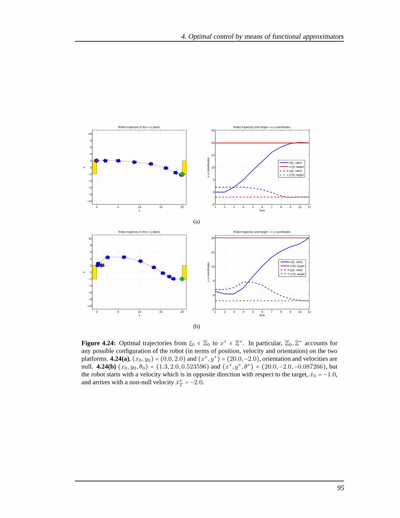
4. Optimal control by means of functional approximators
0 5 10 15 20
−10
−8
−6
−4
−2
0
2
4
6
8
10
x
y
Robot trajectory in the x−y plane.
1 2 3 4 5 6 7 8 9 10 11−5
0
5
10
15
20
25
timex−
y co
ordi
nate
s
Robot trajectory and target− x−y coordinates.
x(t): robotx*(t): targety(t): roboty*(t): target
(a)
0 5 10 15 20
−10
−8
−6
−4
−2
0
2
4
6
8
10
x
y
Robot trajectory in the x−y plane.
1 2 3 4 5 6 7 8 9 10 11−5
0
5
10
15
20
time
x−y
coor
dina
tes
Robot trajectory and target− x−y coordinates.
x(t): robotx*(t): targety(t): roboty*(t): target
(b)
Figure 4.24: Optimal trajectories fromξ0 ∈ Ξ0 to x∗ ∈ Ξ∗. In particular,Ξ0,Ξ∗ accounts for
any possible configuration of the robot (in terms of position, velocity and orientation) on the twoplatforms.4.24(a), (x0, y0) = (0.0,2.0) and(x∗, y∗) = (20.0,−2.0), orientation and velocities arenull. 4.24(b)(x0, y0, θ0) = (1.3,2.0,0.523596) and(x∗, y∗, θ∗) = (20.0,−2.0,−0.087266), butthe robot starts with a velocity which is in opposite direction with respect to the target,x0 = −1.0,and arrives with a non-null velocityx∗T = −2.0.
95

−3 −2 −1 0 1 2 3−3
−2
−1
0
1
2
3
x [m]
y[m
]
0 10 20 30−2
−1
0
1
2Cartesian x
Pos
itio
n[m
]
0 10 20 30−2
−1
0
1
2Cartesian y
0 10 20 30−0.4
−0.2
0
0.2
0.4
time instants
Vel
ocit
y[m
/s]
0 10 20 30−1
−0.5
0
0.5
1
time instants
Figure 4.25: FH neural trajectories, where the difference between the robot and the target’s con-figuration is driven to zero inN steps. Each trajectory is found using the outcome of a sequenceof N neural control functions, after106 training steps and as many robot and target samples. Thered circles are the starting points in the Cartesian space. Some examples of FH trajectories in theplanar space are shown.
96

4. Optimal control by means of functional approximators
−3 −2 −1 0 1 2 3−3
−2
−1
0
1
2
3
x [m]
y[m
]
0 20 40 60 80−2
−1
0
1
2Cartesian x
Pos
itio
n[m
]
0 20 40 60 80−2
−1
0
1
2Cartesian y
0 20 40 60 80−0.4
−0.2
0
0.2
0.4
time instants
Vel
ocit
y[m
/s]
0 20 40 60 80−1
−0.5
0
0.5
1
time instants
Figure 4.26: RH neural trajectories, using the first neural control function of the FH set in Fig-ure 4.25. The same starting points for the trajectories are shown. Here, only the first neural con-troller of the ones used in Figure 4.25 is used to generate theRH control at each time instants.The numerical simulation shows the effect of the RH control law for a longer time with respect tothe fixed horizon used to compute the control functions. Remarkably, the RH controllers are still“active”, though generating null controls, when the targetis reached by the robot.
97

−2 −1.5 −1 −0.5 0 0.5 1 1.5 2
−2
−1.5
−1
−0.5
0
0.5
1
1.5
2
x
yRobot trajectory in the x−y plane.
1
2
3
0 50 100−2
−1
0
1
2RH position x
0 50 100
−2
−1
0
1
RH position y
0 50 100−0.2
−0.1
0
0.1
0.2
0.3RH velocity x
0 50 100−0.5
0
0.5
1RH velocity y
Figure 4.27:The RH controller applied to a mixed tracking/reaching task: the robot moves towarda target which arbitrarily and suddenly changes its position in the state space in an unpredictableway. This case is representative, for example, of the following situation: the mobile robot exploringits workspace (i.e. a room) and while its attentive systems continuously looks for interesting objectsthat the robot must pick up and take somewhere else.
98

4. Optimal control by means of functional approximators
−1 −0.5 0 0.5 1−1
−0.8
−0.6
−0.4
−0.2
0
0.2
0.4
0.6
0.8
1
x
y
Robot trajectory in the x−y plane.
0 50 100−1
−0.5
0
0.5
1RH position x
0 50 100 150−1
−0.5
0
0.5
1RH position y
0 50 100−0.05
0
0.05
0.1
0.15RH velocity x
0 50 100−0.05
0
0.05
0.1
0.15RH velocity y
Figure 4.28: The RH controller applied to a tracking task: the mobile robot follows a target, as-suming a totally unpredictable motion. (even if here, for the sake of simplicity, the target trajectoryhere is a simple circle. This case is representative, for example, of a mobile robot following amoving target, according to a predator-prey paradigm.
99

(as optimality suggests). This is a common problem when training the chain of neural net-works (see hereinafter the discussion in Section 4.5.4): possible causes can be the insufficientnumber of training iteration, or simply the fact the stochastic gradient algorithm stopped at alocal minima and both gradient and descent step cannot make the cost lower any further, andconsequently enhancing the performance of the neural controls. However, dealing with RH,only the first control law is used and the solution of the FH is only preparatory (i.e. we needto solve the complete chain of neural networks, but once found we retain the first and discardthe remaining) so it is possible that even if some control laws are not “optimal” the one neededfor the RH is already “trained”. This is also a consequence ofthe learning algorithm, whichmakes the first neural networks in the chain train faster withrespect to the last ones. In factFigure 4.26 shows the trajectories produced with the RH technique, using the first neural con-troller of the ones used for the FH trajectories in Figure 4.25. It must be noticed that the timeto reach the origin of the planar space is approximately the same of the FH case, and the shapeof the control function is similar also. However, it is important to put in evidence that the RHcontroller remains “active” even when the target is reached: thus, if the robot has reached thetarget, it keeps controlling even if the difference betweenthe two vectors is zero. The latter isan important property, since it shows (in this regulation example) thatγ(0) = 0.
Finally, Figures 4.27 and 4.28 show the RH controller applied in two different trackingtasks: a multiple reaching case and a pure tracking task, where the target is moving unpre-dictably.
4.5.3 A two DOF arm actuated by elastic joints
We consider the following system, describing an arm actuated byn flexible/elastic joints:
M(q)q +N(q, q) +K(q − θ) + J⊺(q)f = 0Bθ +K(θ − q) = τ (4.65)
where for then elastic joints,q ∈ Rn and θ ∈ R
n are the generalized coordinates of thedriven links and actuators. A simplified model is assumed, whereB = diag(b1, . . . , bn) isthe inertia matrix of the actuators,τ ∈ Rn are the motor torques.M(q) is the inertia ma-trix of the manipulator links, whileN(q, q) contains the centrifugal, Coriolis and gravityforces. f is a generic external force field, e.g. a divergent force field, perceived by the end-effector.K is the stiffness matrix, generally symmetric and definite positive: here, we assumeK = diag(k1, . . . , kn), ki > 0∀i. Given the invertibility of the mass matricesM,B, Eq. 4.65can be written as:
q = −M−1(q)N(q, q) −M−1(q)K(q − θ) −M−1(q)J⊺(q)fθ = B−1τ +B−1K(q − θ) (4.66)
which is a control-affine system of the form
x = a(x) + b(x)u + c(x)f (4.67)
where the system state vectorx and the control vectoru arex = col(q, q, θ, θ) andu = col(k, τ)respectively. Of course, (4.67) is in continuous form, and it is straightforward to find its
100

4. Optimal control by means of functional approximators
discrete-time form, for example by applying an Euler’s discretization algorithm. The discrete-time state vector is thenξi = col(qt, qt, qt, θt, θt, θt), t = 0,1, . . . ,N −1, while the control vectoris ut = col(kt, τt), t = 0,1, . . . ,N − 1, and the generic state equation is
ξt+1 = a(ξt) + b(ξt)ut + c(ξt)ft , t = 0,1, . . . ,N − 1Here, the following situation is considered: a two DOF arm (n = 2), performing point-to-
point movements with fixed and known initial and final positions. In this example, all jointshave variable stiffness, thusK is not constant, but in general is a function of timeK = K(t).Indeed, joint stiffness can change in response to differentcommands from the robot controlsystem, as a function of the system configuration or of some motion criteria. The goal is to findthe optimal torque and stiffness profiles that drive the arm from a known initial poseξ∗0 to adesiredξ∗N in N stages, while minimizing a given cost functionJ :
J = N−1∑i=0
Ru2i +Q ξ2i +QN ξ2N
whereR,Q,QN are suitable weight matrices.This motor control problem is formulated as a FH neural reaching problem, described by
Problem 12. The OHL-NN approximating the control laws have6n = 12 inputs and2n = 4
outputs. The following parameters were used to describe thearm dynamics:
• mass:m1 = 1.4, m2 = 1.1• link length: a1 = 0.3, a2 = 0.33• link COM: l1 = 0.11, l2 = 0.16• link inertia: I1 = 0.025, I2 = 0.045
MoreoverB = I, while friction has been neglected (or considered null).Figure 4.29 shows a suboptimal solution, for the caseN = 15, with ∆t = 0.1s. Controls
were generated byN OHL-NN with ν = 5. The cost weights areQ = diag[1,1,0.0001,0.0001, 0, 0],QN = Q, R = diag[0.001]. The stiffness profile is highlighted: notably, its variation during themovement recalls co-contraction, that is the human abilityto change intrinsic musculo-skeletalcompliance. This feature is crucial when dealing with uncertainties and unpredictability in themodel.
4.5.4 Discussion of methods and results
The proposed method is effective and has several advantages, in particular in the capabilityof providing approximating optimal control functions which can be used to implement closedloop control in limited processing and resource machines. The ERIM is potentially capa-ble of managing difficult problems, and the only requirements, preventing its application toFH and RH problems, are the differentiability of all the items involved in the optimizationproblem (state and cost functions, controls, constraints)and the sufficient smoothness of thecontrol functions to be found. However, its effectiveness is evident only if the complexityof the problem is “small”. It is true that other nonlinear optimization methods show simi-lar limitations when dealing with NMPC schemes. However, two are the main drawbacks.
101

−0.2 −0.1 0 0.1 0.2 0.3 0.4−0.1
0
0.1
0.2
0.3
0.4
0.5
start
end
tt
x
y
0 5 10 150
10
20
30
time instants
join
t st
i!n
ess
[N
m/r
ad
]
k1
k2
0 5 10 15−20
−10
0
10
20
time instants
join
t to
rqu
es
[Nm
]
τ1
τ2
Figure 4.29: A point-to-point neural suboptimal trajectory, for a 2DOF arm actuated by elasticjoints. The graphs show the control trajectories of variable joint stiffness and torque.
102
4. Optimal control by means of functional approximators
First the optimal solutions are approximated: local as wellas global optima are possible,and it is not possible to distinguish a local from the (or a) global solution during and afterthe training phase. Second, the stability of the weight update cannot be guaranteed, sincea precise analytical condition is missing. It is possible topartially overcome these two is-sues in practice by re-training the chain of neural networksmultiple times, with differentvalues of its update parameters, i.e. changing the learningstepsize, the initialization ruleof weights and biases, etc. This approach has been adopted also for Neural Dynamic Opti-mization [Seong and Widrow, 2001a, Seong and Widrow, 2001b,Seong and Widrow, 2001c],which face the same issues (the two methods are similar). In practical terms, many issues oc-cur, and cannot be neglected since the method has been presented as a universal one and one ofthe most convenient in solving such optimization problems.
The “curse of dimensionality”
The ERIM is preferred over DP because it can manage a significant number of parameterswithout incurring in the COD, i.e. the exponential growth ofthe number of parameters withthe complexity of the problem. In Section 4.2, the polynomial growth with respect to thenumber of parameters was discussed.
The number of parameters to handle is but considerable, and is due to the following facts.
• A plausible sequence of controls must be provided. The numberN of neural networksconstituting the “chain” and providing controls at each time instant (t, t+1, . . . , t+N −1)must be chosen considering a finite-time movement (i.e. steering the robot from a startingconfiguration to a final one) and the controls frequency. Two issues arise. If the frequencyis high, i.e. ∆t is in the order ofms, hundreds or thousands of time instants must beconsidered, each corresponding to a “neural” element in thechain.
Example 2. The end-effector must perform a movement inT seconds, and controls aresent each∆t ms. For ∆t = 5ms andT = 1,5,10,20s the number of “neural” elementsin the chain is200,1000,2000, 4000 respectively.
The second problem is the fact that the duration of the longest movement should beconsidered in order to set the FH problem properly: unfortunately, the maximum durationcannot be predicted a priori, because it can be context or task dependent (e.g. if you wantto catch a moving object, the movement is fast and can last fewseconds; conversely aprecise pre-grasp movement can last many seconds). In particular, for a FH controller itis fundamental since a too small number of controlsN could lead to control sequenceswhich are not able to drive the end-effector to the desired position correctly.
• The NN must have a sufficient number of parameters to approximate correctly the de-sired optimal control function. In our framework, the function γ to be approximatedis the unknown. With the ERIM, we constrain the function to take on a parameterizedstructure, such that the NN can approximate any possible desired function, but there isno indication on the nature nor on the “shape” of the admissible control function. Theunderlying assumption is that the control function is continuous and differentiable, so
103

that it can be approximated by the NN: in general, the smoother the function, the easiestthe approximation (i.e. less parameter are necessary to approximate it).
Example 3. Suppose a polynomialy(t) = ∑Ni=0 cit
i is used to interpolate a functionf(t)from noiseless data. If the function is a line, theoretically then only two parameters arenecessary, as it can be described by the equationy(t) = c0 + c1t. If the function is acubic, then more are necessary, beingy(t) = c0 + c1t + c2t2 + c3t3. The more complexthe function, the more parameters are necessary.
Remark 13. Some functions are “hard” to approximate with few parameters, e.g. Heav-iside’s step function, Dirac delta-like splines. In general, rough derivatives require moreparameters, or more basis functions.
A specific theorem assessing the number of parameters of an OHL-NN necessary toapproximate a certain function does not exist. However, bounds exist and are mainlyrelated to the smoothness properties of the function to be approximated.. If there are noa priori hypothesis on the “shape” of the control functions, and onlydifferentiability isassumed, then the number of “neurons” for each OHL-NN must bechosen accordingto some practical heuristics. For example, one can solve multiple instances of the sameproblem, augmenting the number of parameters progressively until certain performancesare met.
In general, given an OHL-NN withν neurons,n inputs,m outputs, the total number ofparameters isNν = (n + 1)ν + (ν + 1)m. The “chain” used to solve a FH problem containsT /∆t neural elements. In this configuration the total number of parameters is:
Ntot = TNν
∆t= T (n + 1)ν + T (ν + 1)m
∆t(4.68)
which grows linearly withν. Still, its growth is not negligible with the problem complexity,and even for a simple problem (like the control of a two or three DOF robot) it is enough largeto invoke a COD issue. A graphical representation of the growth of the number of parametersNtot with respect to the problem complexity is shown in Figure 4.30: it can be clearly seen thatin a practical situation where∆t = 5ms,T = 10s andν = 200, the total number of parametersis about 4 millions!
Training a chain of neural networks is “hard”
Another drawback is the training complexity, which is a combination of the effects of thenumber of parameters, the back-propagation algorithm, andstochastic gradient. For the sakeof simplicity, the stochastic element will be discussed later on, and here the focus is only onthe back-propagation algorithm. Denoting asoF , oB the number of operations required for asingle forward and backward phase (on a single NN) respectively, T /∆t the number of neuralelements in a chain, andK the number of iterations of the algorithm to compute the optimalparameters, the total number of operations for the trainingphase is:
otrain = T K
∆t(oF + oB)
104

4. Optimal control by means of functional approximators
which encounters the same problem mentioned for the growth of Ntot. Moreover, since thealgorithm autonomously stops only if the global optimum is reached, or a local one has beenreached and a certain stop condition is verified, the number of iterationsK is practically un-known, but usually very large. In addition, there is not the guarantee that a single instance ofthe learning algorithm (one “shoot”, i.e. one instance given the random initialization of theparameters and a specific data set) can lead to the solution: actually it is common practice to“re-train” the chain multiple times, changing the learningparameters, e.g. changing the descentrule, the regularization terms, etc., or launching in parallel multiple shoots of the optimizationalgorithm. Sometimes the neural networks are “stuck”, immovable in flat regions where thecost function has a very smooth gradient, so that even considerable changes in the stepsize donot lower the cost. This is a known problem in literature [Gori and Tesi, 1992] and so far anumber of heuristics have been suggested, like simulated annealing techniques which basicallyperturb the descent. However, in a stochastic context the gradient is already “perturbed” andsometimes these techniques are not of any use, like discussed in [Spall, 2003].
Training a chain of neural networks in a stochastic context is “harder”
If training a chain of neural networks and system blocks is hard in a deterministic context, it iseven harder to do it in a stochastic context. Difficulties areevident in the simplest case whenonly the initial state is stochastic, i.e. the initial statetakes values from a finite set,ξ0 ∈ Ξ0,according to a certain known distribution:
• Because of stochastic steepest descent, it is not guaranteed that the expected costFalways decreases during training. Recalling the stochastic gradient technique from Sec-tion 4.2.3, since∇F cannot be computed exactly, the gradient coming from a singlerealization of the stochastic variables is used. This meansthat at each iteration step a“perturbed” gradient is used, instead of the correct one. Itis possible to use a betterapproximation of the gradient, computing its expected value over a certain numberM ofrealizations of the stochastic variable, i.e.
∇J ≈ 1
M
M∑h=1
∇J (η(h),w(k))where at iteration stepk, for the current weightsw(k), M realizations of the stochasticvariables vectorη are computed, and forward and backward phases are performedon thechain of neural networks with fixed parametersw(k), so that it is possible to computean average of all the partial derivatives. Obviously,M must be set balancing the benefitsof a better gradient with the computational burden which is introduced by makingMadditional forward-backward phases. Additional ways to address the problem of globalminima of stochastic functions can be found in [Spall, 2003].
• A large number of training, test and validation data is required. The cost functionaldepends on a set of stochastic variables, whose probabilistic distributions are known.Thus, a significant amount of data is required, because we need to sample properly thewhole space of stochastic parameters. If, as frequently happens, the stochastic variable is
105

the initial (or desired) system state (or both), then a suitable sampling of the state space isrequired, taking into account the dimension of the space as well as the resolution (i.e. theminimum distance for which two samples are considered as “different”) and the samplesdistribution.
Example 4. Consider a state space of unitary dimension (n = 1) where the state variableθ is an angle, e.g. defining the orientation of a mobile robot with respect to a fixed frame.The variable range is[0,2π]. Calling θs the sampling resolution, the number of samples(if the sampling is uniform) isNsamples = 2π
θs. If the dimension of the state space is
n, supposing all the variables are of the same type, then the total number of uniform
samples isNsamples= [2πθs ]n. A graphical representation is shown in Figure 4.31: note
that in a practical situation where for examplen = 6 andθs = π/180, Nsamplesis in theorder of1015!
In general, if the dimension of the state space isn andM the number of samples in asingle dimension (supposing the same number of samples for each state variable), thetotal number of samples is at leastNsamples= Mn. The quality of the data set mayalso influence the learning phase. Not only a significant number of data is required,but the sampling type may also affect the training process. In [Fumagalli et al., 2010a]a dissertation on the difference between uniform sampling and random sampling fordifferent machine learning methods was presented. In particular, a random samplingmethod was compared to a selective one, where a certain “sparsity” of the training setwas guaranteed taking a subset, such that the inter-sample distance (computed as theEuclidean distance between the two samples in the standardized input space) was atleast bigger than a certain threshold. Experimental results showed that the two methodsperform identically for large training sets: the difference between the two was evidentonly for small amounts of data (very small, considering the problem dimension). A plotabout such performances is shown in Figure 4.32.
Initialization of the NN affects the optimization algorith m
Finally, the initialization of the networks certainly plays a role. A randomized initialization is“correct” from a theoretical point of view, since it provides an unbiased starting point for thesteepest descent algorithm: having multiple shootings (i.e. multiple instances of the learningalgorithm, for different randomized initial conditions) enhances the chance to lead to the globalminima avoiding the local ones. However, if there exist hypotheses on the “shape” of the con-trol laws, it is possible to exploit such information to “pre-shape” the approximating networks,e.g. to initialize with a suboptimal solution. In this case,a classical Least Squares algorithmcan be used to train the NN [Hagan and Menhaj, 1994], which consists of the following steps:
1. Generate (or measure)L different stochastic variables, such as desired stateξ∗ ∈ Ξ∗:ξ∗(0), . . . , ξ∗(L − 1).
2. For each realizationξ∗(`), solve the corresponding T-stage optimal control problem(which is deterministic, if the stochastic variables are fixed) and find the deterministicsequence of optimal controlsu0(`), u1(`), . . . , uT−1(`)
106

4. Optimal control by means of functional approximators
3. Train theT neural networks with a least-square based method: that is, train thet-thneural network with the training set(ξt(0), ut(0), . . . , (ξt(L − 1), ut(L − 1))
At the end of the aforementioned procedure, each NN is initialized so as to minimize the least-square error between its prediction and the output from the training set. Basically, this methodsimply initialize the network with a suboptimal solution found with a supervised learning tech-nique.
107

0 50 100 150 200 250 300 350 4000
2
4
6
8
10
12
14
15x 10
6
ν
Nto
t
T = 1s T = 5s T = 10s T = 20s
Figure 4.30: The growth of the total number of parameters to be optimized,Ntot, with respect tothe FH problem complexity: the number of neuronsν, the duration of motion (in seconds)T . Here,∆t = 5ms,n = 6,m = 2.
0 1 2 3 4 5 6 7 8 9 1010
0
105
1010
1015
1020
1025
1030
1035
1040
1045
1050
θs [degrees]
Nsa
mple
s
n = 1 n = 4 n = 6 n = 8 n = 14
Figure 4.31: The growth of the number of data samples, when the variable isan angle, and itsrange[0,2π] is uniformly sampled. The number grows exponentially with the dimension of thedata spacen. Note that they axis has a logarithmic scale.
108

4. Optimal control by means of functional approximators
100 100060 5000500 2000200
0.01
0.02
0.03
0.04
0.05
0.06
0.07
0.08
0.09
Training set dimension
NM
SE
RandomEuclidean PVAEuclidean P
Figure 4.32: Comparison of random and selective subsampling based on standardized Euclideandistance. This image is taken from [Fumagalli et al., 2010a], where the input space of a simplemapping problem (mapping joints position, velocities and accelerations with forces and torquesmeasured by a proximal sensor) was randomly or uniformly sampled. EuclideanP and EuclideanPV A denote subsampling based on Euclidean distance in the standardized input space (usingonly position or using position-velocity-acceleration).The performance index was the Normal-ized Mean Squared Error (NMSE) computed on a common validation set. The evidence is that thetwo different subsampling strategies are equivalent for large training sets. The Euclidean-basedsampling outperforms for small data-sets, while the two methods perform nearly identically withthe increase of the data-set.
109

110

Chapter 5
Motion control on humanoids
5.1 A closed loop control scheme
In Section 4.4 a general approach foroptimal neural motor controlwas presented. More pre-cisely, it was shown that a neural approximation of FH and RH control laws can be exploitedfor optimal planning in a tracking/reaching control scheme, satisfying some performance cri-terion. It was shown that it is possible to concentrate all the resource demanding computationsin an offline phase, and to retrieve almost instantly the controls online, taking into account thefeedback on the current status of the system.
In Section 4.5 several examples for different robots were presented. Trajectories were con-veniently planned in the task space (e.g. the Cartesian space), and the optimization procedureprovided the optimal control lawγ (and consequently controlsu(t)), either found using aFH or RH paradigm, and the optimal system state trajectory. An example of planning in jointspace was also discussed, where the dynamics of the robot wasfundamental to the task.
In this chapter we will discuss how to combine the neural optimal motion planning with ahumanoid robotics control scheme. As anticipated in Chapter 2, most humanoids robots canbe controlled through a series of control layers, where different control loops are integrated.In particular, two are the principal methods to control the robot from a “high” level: sendingjoint velocity commands, or joint torques commands. At lower level (i.e. on the boards) eachcontrol type is converted into suitable commands for the actuators, but let us just considerthe aforementioned controls as the ones “supported” by the platforms and their architecturewithout entering into the details of the low level control.
In the above control problems, it was assumed that the desired trajectory was expressed inthe joint space or in the task space, and in the latter case that an equivalent description in termsof joint positions, velocities and acceleration was implicitly available. In humanoids robotics,if the desired trajectory for the end-effector is specified in the operational space, it is necessaryto interpose some Inverse Kinematics (IK) module to transform operational space referencesinto the corresponding joint space references. If torque control is enabled, a Forward Dynamics(FD) module can further translate them into suitable joint torque commands.
In Figure 5.1, a conceptual scheme combining the neural planning module with IK andFD is shown (where iKin and fDyn represent the IK and FD modulerespectively). Both IK
111
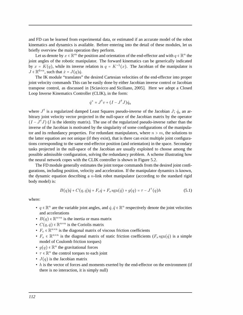
and FD can be learned from experimental data, or estimated ifan accurate model of the robotkinematics and dynamics is available. Before entering intothe detail of these modules, let usbriefly overview the main operation they perform.
Let us denote byx ∈ Rm the position and orientation of the end-effector and withq ∈ Rn thejoint angles of the robotic manipulator. The forward kinematics can be generically indicatedby x = K(q), while its inverse relation isq = K−1(x). The Jacobian of the manipulator isJ ∈ R6×n, such thatx = J(q)q.
The IK module “translates” the desired Cartesian velocities of the end-effector into properjoint velocity commands This can be easily done by either Jacobian inverse control or Jacobiantranspose control, as discussed in [Sciavicco and Siciliano, 2005]. Here we adopt a ClosedLoop Inverse Kinematics Controller (CLIK), in the form:
q∗ = J†v + (I − J†J)qawhereJ† is a regularized damped Least Squares pseudo-inverse of theJacobianJ ; qa an ar-bitrary joint velocity vector projected in the null-space of the Jacobian matrix by the operator(I − J†J) (I is the identity matrix). The use of the regularized pseudo-inverse rather than theinverse of the Jacobian is motivated by the singularity of some configurations of the manipula-tor and its redundancy properties. For redundant manipulators, wheren > m, the solutions tothe latter equation are not unique (if they exist), that is there can exist multiple joint configura-tions corresponding to the same end-effector position (andorientation) in the space. Secondarytasks projected in the null-space of the Jacobian are usually exploited to choose among thepossible admissible configuration, solving the redundancyproblem. A scheme illustrating howthe neural network copes with the CLIK controller is shown inFigure 5.2.
The FD module generally estimates the joint torque commandsfrom the desired joint confi-gurations, including position, velocity and acceleration. If the manipulator dynamics is known,the dynamic equation describing an-link robot manipulator (according to the standard rigidbody model) is:
B(q)q +C(q, q)q + Fv q + Fs sgn(q) + g(q) = τ − J⊺(q)h (5.1)
where:
• q ∈ Rn are the variable joint angles, andq, q ∈ Rn respectively denote the joint velocitiesand accelerations
• B(q) ∈ Rn×n is the inertia or mass matrix• C(q, q) ∈ Rn×n is the Coriolis matrix• Fv ∈ Rn×n is the diagonal matrix of viscous friction coefficients• Fs ∈ Rn×n is the diagonal matrix of static friction coefficients (Fs sgn(q) is a simple
model of Coulomb friction torques)• g(q) ∈ Rn the gravitational forces• τ ∈ Rn the control torques to each joint• J(q) is the Jacobian matrix• h is the vector of forces and moments exerted by the end-effector on the environment (if
there is no interaction, it is simply null)
112
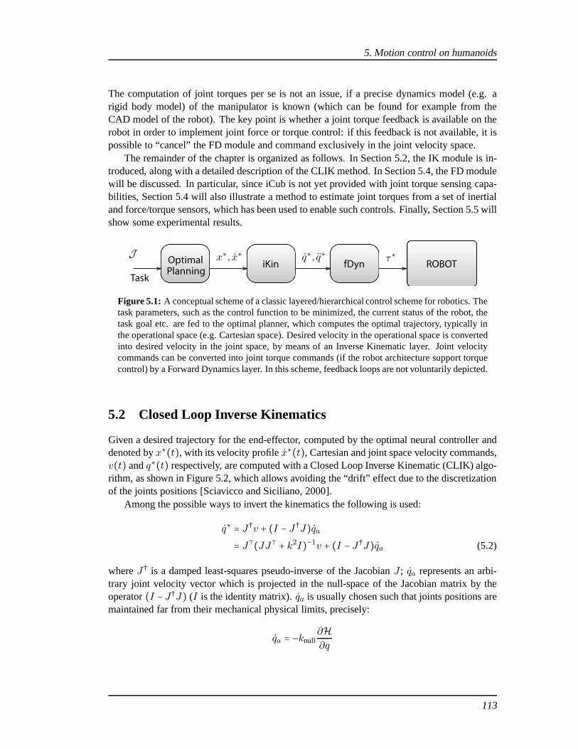
5. Motion control on humanoids
The computation of joint torques per se is not an issue, if a precise dynamics model (e.g. arigid body model) of the manipulator is known (which can be found for example from theCAD model of the robot). The key point is whether a joint torque feedback is available on therobot in order to implement joint force or torque control: ifthis feedback is not available, it ispossible to “cancel” the FD module and command exclusively in the joint velocity space.
The remainder of the chapter is organized as follows. In Section 5.2, the IK module is in-troduced, along with a detailed description of the CLIK method. In Section 5.4, the FD modulewill be discussed. In particular, since iCub is not yet provided with joint torque sensing capa-bilities, Section 5.4 will also illustrate a method to estimate joint torques from a set of inertialand force/torque sensors, which has been used to enable suchcontrols. Finally, Section 5.5 willshow some experimental results.
PlanningTask
Optimal iKin fDyn ROBOTJ x∗, x∗ q∗, q∗ τ∗
Figure 5.1: A conceptual scheme of a classic layered/hierarchical control scheme for robotics. Thetask parameters, such as the control function to be minimized, the current status of the robot, thetask goal etc. are fed to the optimal planner, which computesthe optimal trajectory, typically inthe operational space (e.g. Cartesian space). Desired velocity in the operational space is convertedinto desired velocity in the joint space, by means of an Inverse Kinematic layer. Joint velocitycommands can be converted into joint torque commands (if therobot architecture support torquecontrol) by a Forward Dynamics layer. In this scheme, feedback loops are not voluntarily depicted.
5.2 Closed Loop Inverse Kinematics
Given a desired trajectory for the end-effector, computed by the optimal neural controller anddenoted byx∗(t), with its velocity profilex∗(t), Cartesian and joint space velocity commands,v(t) andq∗(t) respectively, are computed with a Closed Loop Inverse Kinematic (CLIK) algo-rithm, as shown in Figure 5.2, which allows avoiding the “drift” effect due to the discretizationof the joints positions [Sciavicco and Siciliano, 2000].
Among the possible ways to invert the kinematics the following is used:
q∗ = J†v + (I − J†J)qa= J⊺(JJ⊺ + k2I)−1v + (I − J†J)qa (5.2)
whereJ† is a damped least-squares pseudo-inverse of the JacobianJ ; qa represents an arbi-trary joint velocity vector which is projected in the null-space of the Jacobian matrix by theoperator(I − J†J) (I is the identity matrix).qa is usually chosen such that joints positions aremaintained far from their mechanical physical limits, precisely:
qa = −knull∂H∂q
113

ROBOT
−
etR(s) vt
x∗t
q∗tJ†
farm
qt
xrt
x∗t
Figure 5.2: A simple CLIK scheme. The blockJ† refers to (5.2). The retrieving of the target’scartesian coordinates is not modeled, as it would require todiscuss the robotic visual system, thetarget identification module etc. For the sake of simplicity, many details about the closed loopcontrol are voluntarily neglected, to keep the scheme clear, e.g. the computation of the feed-forward command is not detailed.
which minimize the cost function
H(q) = 1
2
N∑i=1
( qi − qi
qmaxi − qmin
i
)where[qmin
i , qmaxi ] is the range for thei-th joint, andqi its midpoint. In such manner it is possi-
ble to cope with singularities and to exploit the intrinsic redundancy of the manipulator. The pa-rameterk2 in (5.2) can be determined adaptively in different ways, forexample using the con-dition number of the Jacobian matrix or the manipulability measure [Chiaverini et al., 2008].In [Sugihara, 2009] a pseudo-inverse Jacobian based on the Levenberg-Marquardt formula wasproposed, where the damping factor was found considering the position/orientation error andthe singular value decomposition of a suitable weighted Jacobian. The algebraic operationyielded smallest joint deviations in the proximity of the singular configuration of the redundantarm, however the author himself pointed out that the method could lead to physically unfeasi-ble motions, as the continuity of the solution was not preserved. Here1, we prefer the methodproposed in [Chiaverini et al., 1991], wherek depends on the smallest singular valueσmin ofthe Jacobian matrix:
k2 = ⎧⎪⎪⎨⎪⎪⎩0 σmin > σ[1 − (σmin
σ)2]k σmin < σ . (5.3)
For example, in James we setσ = 0.20 andk = 0.10, after manually driving the arm to singularconfigurations and studying the singular values, and setting a safety threshold. In fact, it mustbe pointed out that the smallest singular value can be lower than the thresholdσ even in non-singular configurations of the arm.
Note that the singularity is solved by acting on the singularvalues, which are configuration-dependent, while redundancy is resolved by selecting the solution which stays furthest awayfrom the joints bounds. A point-wise approach like this may not lead to the best solution forthe overall trajectory. It is reasonable to solve the IK thisway, since “globally” the controlfunctions are already an approximation of the global ones, and the smoothing properties of theneural networks should prevent rough behaviors.
1All cited method were evaluated: best results were found using (5.3).
114

5. Motion control on humanoids
ROBOT
−
etR(s)
µ
vt
x∗t
q∗t
J†
farm
qt
xrt
x∗t
xgt
J
Figure 5.3: James’s arm CLIK controller, with the contribution, in evidence, of the neural con-troller.
The generation of the commanded Cartesian velocitiesv(t) in (5.2) is shown in Figure 5.2.With an abuse of notation2, v(t) = x∗(t) +R(s) ∗ e(t), wheree(t) = x∗(t) − x(t) andR(s)a regulator which will be discussed hereinafter. The classical CLIK scheme relies on a purelyproportional regulator, i.e.R(s) = Ke, whereKe is a diagonal positive defined matrix. In anideal situation, the correction termKee(t), wheree(t) = x∗(t)−x(t), guarantees convergenceto zero of the Cartesian error and the error dynamice +Kee = 0 is asymptotically stable. Theconvergence velocity of such system depends on the eigenvalues of the gain matrixKe > 0
[Chiaverini et al., 2008, Sciavicco and Siciliano, 2000].When the robot is performing tracking tasks, the discrete-time system must respond to
rapid variations of the target trajectory: hence, the gainKe should be raised until some rea-sonable performances are met. Unfortunately,Ke cannot be raisedad libitum: its upper-limitis determined by the physics of the problem, and high-frequency terms, delays and unmod-eled dynamics also prevent to increaseKe to a desired value. For these reasons the simpleproportional gainKe is substituted with the following:
R(s) =Ke1 + sτe
s(5.4)
whereKe is still a positive diagonal matrix,τe a time constant. Incidentally, (5.4) correspondsto a PI controller, where the proportional gain isKeτe and the integral one isKe. The samplingtime ∆t is then fundamental for the proper tuning of the digital integral gain. The time con-stantτe (corresponding to the zero−1/τe) can be then manually adjusted (e.g. looking at stepand ramp response, and their transient trajectories), so asto raise the proportional gain whilepreserving the system safety.
In general, regulator (5.4) can guarantee asymptotic stability with faster response of thesystem with respect to the purely proportional regulator. The commanded Cartesian velocitiesare then:
v(t) = x∗(t) +Keτee(t) +Ke ∫ e(t)dt. (5.5)
Also in this case, it is possible to guarantee stability and convergence, forτe > 0,Ke > 0 andthe trend of convergence depends on the two eigenvalues resulting from s2 + keτes + ke = 0
(Ke = keI).The semi-global stability of the regulatorR(s) by means of a Lyapunov function can be
also proved. Given a desired trajectoryx∗ ∈ C1, wherex∗(t), x∗ are bounded, define with
2R(s) denotes a Laplace transform of the regulatorR.
115

e(t) ≜ x∗(t)−x(t) the trajectory error, such thate = x∗ − x = x∗ −Jq. Consider the followingcandidate Lyapunov functionV (e) = 1
2e⊺e > 0 (“globally” definite positive, sinceV (0) = 0),
with V = e⊺e = e⊺(x∗ − Jq). Take the following velocity
q = J†(x∗ +Keτee +Ke∫ e(t)dt) ,
then substitute it intoV :
V = e⊺[x∗ − JJ†(x∗ + keτee + ke∫ e(t)dt)]= −e⊺Keτee − e
⊺Ke∫ e(t)dt≤ −keτe ∥e∥2 − keα ∥e∥
whereα ≜ ∫ e(t)dt. Assume that∃α ∶ ∫ e(t)dt ≤ α ∥e∥. If V is a Lyapunov function,i.e. V ≤ 0, thene = 0 is a globally stable equilibrium state. Sinceke, τe > 0, the sign ofαdetermines the stability property. Ifα > 0, then∀ ∥e∥ , V ≤ 0, sinceV is a quadratic function,with V (0) = 0. If α < 0, thenV is still a quadratic function, withV (0) = 0, but V (e) > 0 for0 < ∥e∥ < α
τe: in this region, there is no attractiveness, however it is possible to shorten that
region to a desired, by increasing suitablyτe. In this case,e = 0 is semi-globally stable.
5.3 Forward Dynamics
In Section 5.2 we presented a method for converting desired trajectories in the operationalspace into desired trajectories in the joint velocity space. The latter can be either sent to therobot, to a joint velocity control interface, or further translated into joint torques commands, ifthere is a force/torque control interface is available. Furthermore, desired trajectories can beplanned directly in torque space, considering a nonlinear model of kinematics and dynamics ofthe system. In each of the following cases, it is necessary tocompute the Forward Dynamics ofthe robot, i.e. the mapping between its proprioceptive configuration (joint positions, velocitiesand accelerations) and joint torques. Of course, a suitabledynamics model (e.g. a rigid bodydynamics model) must be known.
The classical dynamic equation describing an-link robot manipulator is described byEq. 5.1. A notable property is the linearity of the model withrespect to the dynamic parameterswhich characterize the manipulator, particularly in the absence of external forces (h = 0) (5.1)can be written as:
τ = Y (q, q, q)π (5.6)
whereY ∈ Rn×p is theregressorandπ ∈ Rp is the vector collecting the set of constant parame-ters which describe the manipulator dynamics [Sciavicco and Siciliano, 2005].
Such parameters, including link mass, inertia, Center of Mass (COM) location, etc., canbe usually retrieved from the CAD model of the robot. Frequently, they are partially known,or known with some uncertainties: in this case, supervised learning techniques such as Sup-port Vector Machines (SVM) and NN can be used either to find thebest set of parameters or
116

5. Motion control on humanoids
to directly approximate the forward dynamics of the robot. An interesting analysis and com-parison of model based versus supervised learning technique for this problem can be found in[Fumagalli et al., 2010a], and will be shortly discussed in Section 5.3.1.
5.3.1 Robot dynamics: model or learning?
The robot dynamics, expressed byY (⋅) in equation Eq. 5.1, can be identified either derivingit analytically, or approximating it using a set of experimental data and a machine learningtechnique. In the latter case, the learning algorithm is agnostic to the underlying dynamicsmodel that is used to produce the examples, but the main advantage is that nonlinear effectsdo not need to be explicitly modeled, as these are learned implicitly by the algorithm. Inthis section3, we will report some significant results about a comparison of the model-basedapproach and two machine learning algorithms, applied to the identification of a robotic armdynamic model:
1. Model-Based Approach
Eq. 5.1 defines torques as a linear product of matrixY (q, q, q) and vectorπ: the firstdepends solely on the joint positions, velocities and accelerations, whereasπ containsthe dynamical parameters that we must estimate to describe the manipulator dynamics[Kozlowski, 1998]. In particular,π is the minimum set of identifiable parameters, i.e. alinear combination of a multitude of elements, containing products among each link massmi ∈ R, inertial parametersIi ∈ R6 (the inertia matrix can be defined by six parametersbecause of its symmetric properties), Center Of MassCi ∈ R3 (COM - in form of adistance vector between the COM frame and the reference frame of the link, eventuallya roto-translational matrix if frames have also different orientations), length, and so on4.The system dynamical parametersπ can be often retrieved from an accurate model ofthe robot (e.g. CAD drawings), but they are not generally accurate, hence a weightedlinear Least Squares technique can be used to improve their estimate. GivenL samples,consisting of measurements(τ`, q`, q`, q`), the set of optimal parameters can be foundas:
π = argminπ
L∑=1
(τ` − Y (q`, q`, q`) π)⊺ω(τ` − Y (q`, q`, q`) π) .
whereω is a suitable weighting diagonal matrix. The explicit solution is given by:
π =∆†Ωτ = [∆⊺Ω∆]−1∆⊺Ωτ ,
whereΩ = diag(ω),∆ = col(Y (q1, q1, q1), . . . , Y (qL, qL, qL)), andτ = col(τ1, . . . , τL).2. Least Squares Support Vector Machines for Regression
3The detailed description of the methods can be found in [Fumagalli et al., 2010a].4Each kinematic chain link has an associated reference frame, defined by the Denavit-Hartenberg convention
[Denavit and Hartenberg, 1955, Lagarde et al., 2009]. All the dynamic and kinematic quantities of each link (COM,inertia, length, etc.) refer to the associated reference frame.
117

Least Squares Support Vector Machines (LS-SVMs) belong to the class of kernel me-thods which use a positive definite kernel function to estimate a linear approximatorin a (usually) high-dimensional feature space [Suykens et al., 2002]. Let us define thedata setS = x`, y`L`=1, where inputsx` ∈ Rn and corresponding outputsy` ∈ R for ` =1, . . . ,L. LS-SVM estimates a linear decision function of the formf(x) = ⟨w,φ(x)⟩+b,whereb is a bias term andφ(⋅) ∶ Rn
↦ Rf maps samples from the input space into a
(usually) high-dimensional feature space. The weight vector w and biasb are chosensuch that both the squared norm ofw and the sum of the squared errorsε` = y` − f(x`)are minimized, which is found by solving a dual optimizationproblem in the form
maximize1
2∥w∥2 + 1
2C
L∑=1
ε2` −L∑=1
α` (⟨x`,w⟩ + b + ε` − y`) ,
whereα` ∈ R are the Lagrange multipliers associated with each sample. The decisionfunction can be rewritten asf(x) = ∑L
`=1α` ⟨φ(x`), φ(x)⟩ + b. Hence, a kernel functionk(xi, xj) = ⟨φ(xi), φ(xj)⟩ can be used to implicitly map the data into the feature space.Given a kernel matrixK = k(xi, xj)Li,j=1, the solution to the optimization problem in(2) is given by a system of linear equations:
[αb] = [K +C−1I 1
1T 0]−1 [y
0] .
which is reduced to a(L + 1) × (L + 1) matrix inversion, solved efficiently by state ofthe art algorithms such as Cholesky decomposition [Cawley,2006].
3. Neural Networks Lastly, a multiple input - multiple output OHL-NN can be used, forits generalization and approximation capabilities [Hornik et al., 1989], and de-noisingproperty when dealing with experimental data. Given a batchdata set, a typical trainingalgorithm for NN is based on the well known Levenberg-Marquardt (LM) algorithm[Levenberg, 1944, Marquardt, 1963], where the criterion for training the network (thatis to find the optimal parametersw) is to minimize the mean squared error between theestimated and the measured data:
w = argminΦ(w) = argmin1
2
L∑i=1
ε⊺` (w)ε`(w) ,
whereε`(w) = τ` − µ(τ`,w) is the error between the measured and the predicted data,estimated by a NNγ(⋅,w), with the same structure seen in Chapter 4. The iterativealgorithm consists in a back-propagation of the error function, to compute its partialderivatives with respect tow, and a weight update equation
wk+1 = wk − [J⊺(wk)J(wk) + µI]−1J⊺(wk)ε(wk) ,
whereε(wk) = [ε1(wk), . . . , εL−1(wk)], andJ(wk) ∈ RL×W is the Jacobian matrix ofthe errors with respect to the parameters of the NN. The parameterµ, adjusted iteratively,balances the LM between a steepest descent and a Gauss-Newton algorithm.
118

5. Motion control on humanoids
Generally, learning algorithms outperform the rigid body dynamic model in terms of pre-diction accuracy, given that a sufficient amount of trainingdata is available. The generalizationperformance of these methods improves steadily as more training samples become available.LS-SVM converges slightly faster than Neural Networks, buttheir final performance on largedata sets is nearly identical. The model-based method, on the other hand, requires very fewsamples to achieve acceptable predictions.
In [Fumagalli et al., 2010a], the three methods have been evaluated experimentally on acommon data set that has been gathered during a sequence of random arm movements, per-formed in joint space by the humanoid robot James. Without entering into the details of theexperiment and the full comparison among the methods, we report here some interesting re-marks:
• Number of Training Samples: the two learning methods have a strong dependency onthe size of the training set. They consistently improve performance with the increase ofthe training set, eventually outperforming the model-based approach by an order of mag-nitude, as shown in Figure 5.4(a); whereas the model-based approach appears to performat a constant level, regardless of the number of samples. This means that the model-basedapproach is the preferred approach when only very few samples are available.
• Contribution of Velocity and Acceleration on the Estimation: including joint veloc-ities and accelerations does not always improve the generalization performance of thelearning methods when training is done on a small number of samples. This is probablydue to the fact that learning algorithms require an increasing amount of training samplesto make effective use of this additional information (i.e. the COD [Duda et al., 2001]).Figure 5.4(b) shows that both LS-SVM and NN use joint velocities to improve their pre-dictions only if given a sufficiently large training set. Joint accelerations do not seemto contribute positively to the estimation, but this is probably caused by the experimentitself, where motions were smooth, and by the fact that accelerations were not measureddirectly but derived from positions (thus, very noisy).
• Selective subsampling: to avoid data oversampling in an abundance of training data, aselective subsampling strategy was designed to remove samples that were nearly identi-cal to each other, which particularly affects LS-SVM performance. A certain “sparsity”of the training set was guaranteed by taking a subset, such that the inter-sample the Eu-clidean distance in the standardized input space was at least a thresholdt. When thisdistance is determined solely based on the joint positions,then Euclidean subsamplingresults in a significant improvement for small data sets. Forlarge data sets, and thus asmall inter-sample threshold, the Euclidean and random subsets have very similar sam-ple distributions and therefore similar performance. In contrast, random subsamplingperforms better than Euclidean subsampling based on joint positions, velocities and ac-celerations. Some results are shown in Figure 5.5.
119

100 100060 200 500 500020000
0.05
0.1
0.15
NM
SE
P − ModelP − LS−SVMP − NN
10060 500 1000 500020002000
0.05
0.1
0.15
NM
SE
PV − ModelPV − LS−SVMPV − NN
100 1000500200 50002000600
0.05
0.1
0.15
Training set dimension
NM
SE
PVA − ModelPVA − LS−SVMPVA − NN
(a)
100 100060 5000500200 2000
0.05
0.06
0.07
NM
SE
P − ModelPV − ModelPVA − Model
100 100060 5000500 2000200
0.06
0.02
0.01
0.005
0.002
NM
SE
P − LS−SVMPV − LS−SVMPVA − LS−SVM
100 100060 5000500 2000200
0.01
0.1
0.02
0.005
0.05
Training set dimension
NM
SE
P − NNPV − NNPVA − NN
(b)
Figure 5.4: Comparison of the three methods on random training subsets of increasing dimension and three different input spaces. Four jointsof James’ arm were involved in the experiment.P denotes the input space containing only joint positions (q ∈ R4), PV contains both jointpositions and velocities (q, q ∈ R8), andPVAcontains joint positions, velocities and accelerations (q, q, q ∈ R12). Note that in5.4(b)both axesare in logarithmic scale to accentuate differences in final performance.
120
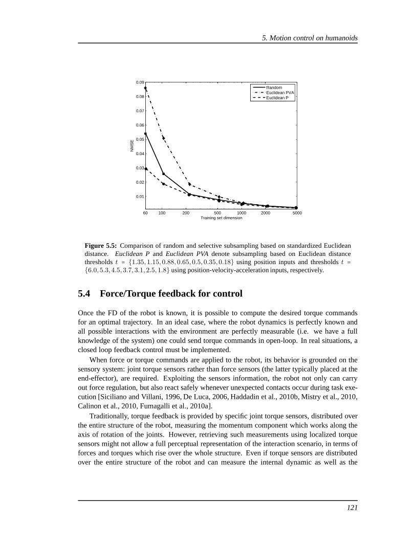
5. Motion control on humanoids
100 100060 5000500 2000200
0.01
0.02
0.03
0.04
0.05
0.06
0.07
0.08
0.09
Training set dimension
NM
SE
RandomEuclidean PVAEuclidean P
Figure 5.5: Comparison of random and selective subsampling based on standardized Euclideandistance. Euclidean Pand Euclidean PVAdenote subsampling based on Euclidean distancethresholdst = 1.35,1.15,0.88,0.65,0.5,0.35,0.18 using position inputs and thresholdst =6.0,5.3,4.5,3.7,3.1,2.5,1.8 using position-velocity-acceleration inputs, respectively.
5.4 Force/Torque feedback for control
Once the FD of the robot is known, it is possible to compute thedesired torque commandsfor an optimal trajectory. In an ideal case, where the robot dynamics is perfectly known andall possible interactions with the environment are perfectly measurable (i.e. we have a fullknowledge of the system) one could send torque commands in open-loop. In real situations, aclosed loop feedback control must be implemented.
When force or torque commands are applied to the robot, its behavior is grounded on thesensory system: joint torque sensors rather than force sensors (the latter typically placed at theend-effector), are required. Exploiting the sensors information, the robot not only can carryout force regulation, but also react safely whenever unexpected contacts occur during task exe-cution [Siciliano and Villani, 1996, De Luca, 2006, Haddadin et al., 2010b, Mistry et al., 2010,Calinon et al., 2010, Fumagalli et al., 2010a].
Traditionally, torque feedback is provided by specific joint torque sensors, distributed overthe entire structure of the robot, measuring the momentum component which works along theaxis of rotation of the joints. However, retrieving such measurements using localized torquesensors might not allow a full perceptual representation ofthe interaction scenario, in terms offorces and torques which rise over the whole structure. Evenif torque sensors are distributedover the entire structure of the robot and can measure the internal dynamic as well as the
121

interaction occurring on their link, they can measure a single component of momentum whichworks along the axis of rotation of the joints. More specifically, since forces and torques arelinearly related by the transposed Jacobian, which might have a non-empty null-space, thereexist singular configurations where some interaction forces at sensory level cannot be fullyretrieved (e.g. pure forces working on a direction which is parallel to the joint torque sensoraxis arehidden).
A more robust and complete representation of the interaction forces can be retrieved byForce/Torque Sensors (FTS). Classically, robots are equipped with six-axis FTS mounted intheir end-effectors, where the most interaction with the environment occurs during manip-ulation [Sciavicco and Siciliano, 2005]. This solution is compact and less invasive with re-spect to the design of joint torque sensors [Parmiggiani et al., 2009, Luh et al., 1983], allowsa complete representation of the interaction and thus the achievement of active compliance[Caccavale et al., 2005, Chiaverini et al., 1999, Sicilianoand Villani, 2000]. However, this in-formation is localized at the tool level. In other words, a FTS at the end-effector does not allowretrieving neither the information about the manipulator dynamics, nor about the potential in-teraction occurring on any link of the robotic system. In this situation, this information mustbe retrieved with other sensors.
If a FTS is located proximally, for example in the middle of a kinematic chain, it is possibleto exploit its measurements in a different way, and basically “propagate” its measures throughthe chain. A simple way consists in “projecting” its measurements on the joints through thetransposed Jacobian. A more complete representation can befound by applying recursivelyNewton’s laws, and will be briefly introduced in Section 5.4.1. However, the analytical solutionfor computing joint torques becomes quite complex for more complicated kinematic structures.
In Section 5.4.2, we describe instead a procedure which allows retrieving a more completeand better representation of the interaction forces over the entire structure of single and multi-branched kinematic chains, such as a humanoid robot. The proposed approach makes use ofthree sets of sensors, distributed along the kinematic chain:
• force/torque, used to measure dynamical wrenches, i.e. the forces and moments that aredue to the dynamics of the structure;
• inertial, since their measurements can be propagated through the chain if the kinematicmodel of the robot is known, thus allow retrieving a completedescription of the kine-matics information of the links in the manipulator;
• finally, distributedtactile sensors provide the information about the location of contactsoccurring dynamically with the environment.
Under suitable assumptions, we will show that by exploitingthese sensors it is possible bothto detect external wrenches and to obtain complete information of the wrenches transmittedalong the structure (and thus also joint torques). Basically, if a precise dynamical model ofthe robot is known (i.e. a rigid body model), internal forcesand torques can be computedby means of recursive algorithms, such as the classicalRecursive Newton-Euler Algorithm(RNEA) [Sciavicco and Siciliano, 2005]. To the best of our knowledge, a similar solution hasbeen adopted only once in [Morel and Dubowsky, 1996, Morel etal., 2000] where a single FTSplaced at the base of a 3 Degrees Of Freedom (DOF) PUMA manipulator was used to estimate
122

5. Motion control on humanoids
−µi+1
−fi+1
fi
µi
Ci
ri−1,Ciri,Ci
⟨i − 1⟩⟨i⟩
Figure 5.6: Notation for thei-th link of a kinematic chain. A more complete description can befound in [Sciavicco and Siciliano, 2005].
the joint torques. In Section 5.5.2, some experiments are shown, where the proposed methodhas been applied to estimate forces and torques on 32 of the 53DOF of the iCub. Moreover, weenrich the estimation by also computing external forces at any contact location. This informa-tion can be fixeda priori for particular robot tasks, but in general must be updated on-the-fly:in iCub it is provided by its “artificial skin”. In the remainder of this section we will introducethe Enhanced Oriented Graph (EOG) method, which is used to perform the RNEA computa-tions on both single and multiple branched open kinematic chains, when one or multiple FTSare available. It must be pointed out that the RNEA is here proposed as a tool to compute kine-matic and dynamic information recursively, but its adoption is not a must and other recursivealgorithms could be used. The proposed method is thus shown to be generic and applicableto every open kinematic tree. Force sensors are used to improve the estimation of the internalwrenches and for the computation of external interaction. The number of FTS to employ andtheir placement along a manipulation structure is not defined. We only suggest spreading themon different links of the system to increase the quality and reliability of the results. The method,in fact, presents a systematic procedure for computingN + 1 external wrenches fromN inter-nal wrenches (i.e. measurements from FTS). Remarkably, under some conditions that will bepresented in next sections, all link wrenches and joint torques can be theoretically computed.
It is necessary to introduce the notation of the variables required for computing the internaland external forces and torques. Given a forcef ∈ R3 and a momentµ ∈ R3, a wrenchw ∈ R6
is the vectorw = col (f,µ). FTS, which actually measure a wrench, are named according tothe physics terminology, whereµ is called torque. To discriminate from the joint torqueτ , wecall µ moment accordingly to the mechanical terminology. The description of the kinematicsand the dynamics of a link (see Figure 5.6) adopts the Denavit-Hartenberg notation. We limitthe discussion to revolute joints for the sake of simplicity, but the method is generic for bothrevolutionary and linear joints. Here is a list of the adopted symbols:
⟨⋅⟩ generic Cartesian reference frameva givenv ∈ Rn a genericn-dimensional vector,va is v expressed in⟨a⟩Rb
a theSO(3) rotation matrix from⟨a⟩ to ⟨b⟩ra,b distance vectorr from ⟨a⟩ to ⟨b⟩
123

zi z-axis of⟨i⟩, aligned with the axis of rotation of jointiθi the angle associated to thei-th jointpi ∈ R3, denotes the linear acceleration of⟨i⟩
ωi, ωi ∈ R3, the angular velocity and acceleration of⟨i⟩mi mass associated with thei-th linkIii ∈ R3×3 represents the inertia tensor of thei-th link, defined with respect to the center of
mass oriented as the frame⟨i⟩Ci ∈ R3 the coordinate vector of the center of mass of linki-th, with respect to⟨i⟩fi ∈ R3, represents the forces applied on⟨i⟩, that link i + 1 exert on thei-th linkµi ∈ R3, represents the moment applied on⟨i⟩, that link i + 1 exert on thei-th linkτi ∈ R the joint torque, i.e. the component ofµi alongziwi ∈ R3 is the wrenchw = ( fµ ) applied on⟨i⟩, that link i + 1 exerts on linki
5.4.1 Wrench transformations and FTS measurements
Consider a kinematic chain, where a FTS is embedded in theiS-th link as shown in Fig-ure 5.8(b). Name the sensor frame⟨s⟩ and number progressively the links frames⟨iS ⟩ , ⟨iS + 1⟩ , . . .as⟨s + 1⟩ , ⟨s + 2⟩ and so on: interestingly, all links wrenchesws+k = [f s+k
s+k , µs+ks+k] can be ex-
pressed as function of the FTS measurementsws = [f ss , µ
ss] by the compact formula:
ws+k = As+k ws + ws+k
τs+k = ws⊺ Cs+k z0 + τs+k
whereAs+k andCs+k basically contain the rotations and distance vectors between frames totransform wrenches between different coordinate frames, specifically:
As+k = [ Rss+k⊺ 0
−Rss+k⊺(rs+k−1s−1,s+k−1)∧ Rs
s+k⊺]
Cs+k = [(rs+k−1s+1,s+k−1)∧ Rss+k−1
Rss+k−1
]
ws+k = [f s+ks+k , µ
s+ks+k] and τs+k instead contain all the dynamic terms which are not taken into
account by simply applying a wrench transformation betweendifferent frames in a rigid-body.Indeed, matrixAs+k is the Adjoint matrix defining a wrench transformation in a rigid body[Murray et al., 1994].
As an example, in the “static” case (i.e. whenqi = qi = 0,∀k) we have:
f s+ks+k = Rs
s+k⊺f ss −
k−1∑j=0
Rs+js+k ms+j p
s+jCs+j
124
5. Motion control on humanoids
µs+ks+k = Rs
s+k⊺µss −R
ss+k⊺ (rs+k−1s−1,s+k−1)∧ f s
s
−
k−1∑j=0
Rs+js+k
⊺ms+j (rs+js+j,Cs+j
)∧ ps+jCs+j
+
k−2∑j=0
Rs+js+k
⊺ms+j (rs+k−1s+j,s+k−1)∧ ps+jCs+j
τs+k = [ Rss+k−1
⊺µss −R
ss+k−1
⊺(rs+k−1s−1,s+k−1)∧ f ss
−
k−1∑j=0
Rs+js+k−1
⊺ms+j (rs+js+j,Cs+j
)∧ ps+jCs+j
+
k−2∑j=0
Rs+js+k−1
⊺ms+j (rs+k−1s+j,s+k−1)∧ ps+jCs+j
⎤⎥⎥⎥⎥⎦⊺
z0
which gives:
⎡⎢⎢⎢⎢⎢⎣f s+ks+k
µs+ks+k
⎤⎥⎥⎥⎥⎥⎦=⎡⎢⎢⎢⎢⎢⎢⎢⎢⎣
−Rss+kmsp
sCs
−Rs+1s+kms+1p
s+1Cs+1
⋯
−Rss+k⊺(rss,Cs
)∧mspsCs
−Rs+1s+k⊺(rs+1s+1,Cs+1
)∧ms+1ps+1Cs+1
⋯
−Rss+k⊺(rs+k−1s,s+k−1)∧msp
sCs−Rs+1
s+k⊺(rs+k−1s+1,s+k−1)∧ms+1p
s+1Cs+1
⋯ −Rs+k−2s+k ms+k−2p
s+k−2Cs+k−2
−Rs+k−1s+k ms+k−1p
s+k−1Cs+k−1
⋯ −Rs+k−2s+k−1
⊺(rs+k−2s+k−2,Cs+k−2)∧ms+k−2p
s+k−2Cs+k−2
−Rs+k−1s+k−1
⊺(rs+k−1s+k−1,Cs+k−1)∧ms+k−1p
s+k−1Cs+k−1
−Rs+k−1s+k
⊺(rs+k−1s+k−2,s+k−1)∧ms+k−2ps+k−2Cs+k−2
⎤⎥⎥⎥⎥⎥⎥⎥⎥⎦and the following torques:
τs+k =
⎡⎢⎢⎢⎢⎢⎢⎢⎢⎢⎢⎢⎢⎢⎣
ms(psCs)⊺ (rss,Cs
)∧ −ms (psCs)⊺ (rs+k−1s,s+k−1)∧ Rs
s+k−1
⋮
ms+k−2(ps+k−2Cs+k−2)⊺ (rs+k−2s+k−2,Cs+k−2
)∧ Rs+k−2s+k−1+
−ms+k−2(ps+k−2Cs+k−2)⊺ (rs+k−1s+k−2,s+k−1)∧ Rs+k−2
s+k−1
ms+k−1(ps+k−1Cs+k−1)⊺ (rs+k−1s+k−1,s+k−1)∧ Rs+k−1
s+k−1
⎤⎥⎥⎥⎥⎥⎥⎥⎥⎥⎥⎥⎥⎥⎦
z0
The “dynamic” case (i.e. when joint velocities and accelerations are not zero, thus duringmotion) is not explicitly reported for the sake of brevity and simplicity, because the equationsbecome much more complicated. However, even in that case thejoint torques can be retrievedjust applying the aforementioned formulas recursively.
125

v0 v1 vn
⟨0⟩ ⟨1⟩ ⟨n⟩
e0,1 en−1,ne1,2
Figure 5.7: An open chain represented as a graph.
5.4.2 Enhanced Oriented Graphs
Graph theory has been extensively used to represent mechanical systems [Wittenburg, 1994,Featherstone and Orin, 2008] and kinematic chains, producing compact and clear models, inmatrix forms with beneficial properties (e.g. branch-induced sparsity [Featherstone, 2010])when the connectivity among its elements is expressed. There is not a unique choice for agraph representing a chain: for example, in [Featherstone,2007] graphs are undirected, nodesand arcs represent bodies and joints respectively; the resulting graph is undirected (i.e. non-oriented), but nodes are “labeled” according to a “regular numbering scheme”.
This section presents the theoretical framework of theEnhanced Oriented Graphs(EOG),applied to the computation of both internal and external wrenches applied to single and multiplebranches, generally non-grounded, kinematic chains. The proposed method is an extension ofthe classical RNEA [Featherstone and Orin, 2008, Sciaviccoand Siciliano, 2005]. Similarly tothe classical approach we represent a kinematic chain as a graph such that computations ofthe system dynamics can be obtained performing a pre-order and a post-order traversal visit ofthe graph itself. However, we enhance the graph with specificnodes representing both knownand unknown (kinematic or dynamic) variables. Remarkably,not all the unknowns will bespecified a-priori (e.g. contacts at arbitrary locations might appear and other contacts mightbe removed) and therefore the graph structure will be adapted accordingly5. This dynamicallyevolving graphical description of the chain modifies the waythe graph is visited during theNewton-Euler recursion, thus changing in particular the direction along which the recursionis propagated in the graph. In order to cope with this evolving representation we introducedanother difference with respect to previous RNEA graphicalrepresentations by representingthe kinematic chain as anorientedgraph: the direction along which edges are traversed willdetermine either the use of the classical Newton-Euler recursion formula or a slightly modifiedversion of it.
The enhanced graph representation
We here consider an open (single or multiple branches) kinematic chain withn DOF composedof n + 1 links.
Adopting the Denavit-Hartenberg notation [Sciavicco and Siciliano, 2005], we define a setof reference frames⟨0⟩, ⟨1⟩, . . . , ⟨n⟩ attached at each link.
5Within this context, a crucial role is played by the distributed tactile sensor, primarily used to compute thepresence and the location of externally applied wrenches. Even if the tactile sensor would be capable of measuringalso the component of the force normal to the skin surface, this information is not used in this paper where we focuscomputing both the applied force and torque (i.e. the whole externally applied wrench) exploiting the embeddedsensors.
126

5. Motion control on humanoids
The i-th link of the chain is described by a vertexvi (sometimes called node), usuallyrepresented with the symboli©. A hinge joint between the linki and the linkj (i.e. a rotationaljoint) is represented by an oriented edgeei,j connectingvi with vj: i©→ j©. In an DOF openchain, each vertex (except for the initial and terminal,v0 andvn respectively) has two edgeconnections. Therefore, the graph representation of then-links chain is an oriented sequenceof nodesvi, connected by edgesei−1,i.
The orientation of the edges can be either chosen arbitrarily (it will be clear later on thatthe orientation simply induces a convention) or it can follow from the exploration of the kine-matic tree according to the “regular numbering scheme” [Featherstone and Orin, 2008], whichinduces a parent/child relationship such that each node hasa unique input edge and multipleoutput edges. Following the classical RNEA and the classical Denavit-Hartenberg notation, weassume that each joint has an associated reference frame with thez-axis aligned with the rota-tion axis; this frame will be denoted⟨ei,j ⟩. In kinematics, an edgeei,j from vi to vj representsthe fact that⟨ei,j ⟩ is fixed in thei-th link. In dynamics,ei,j represents the fact that the dynamicequations will compute (and make use of)wi,j , i.e. the wrench that thei-th link exerts on thej-th link, and not the equal and opposite reaction−wi,j, i.e. the wrench that thej-th link exertson thei-th link (further details in Section 5.4.2). In order to simplify the computations of theinverse dynamics on the graph (see Section 5.4.2), kinematic and dynamic measurements havebeen explicitly represented. Specifically, the graph representation has been enhanced with anew set of graphical symbols: a triangle to represent kinematic quantities (i.e. velocities andacceleration of links –ω, ω, p), and a rhombus for wrenches (i.e. force sensors measurementson a link –f , µ). Moreover these symbols have been further divided intoknownquantities torepresent sensors measurements, andunknownto indicate the quantities to be computed, as inthe following:
• : unknown kinematic information• : known (e.g., measured) kinematic information• ◊: unknown dynamic information• ⧫: known (e.g., measured) dynamic information
Kinematic variables can in general be measured by means of gyroscopes, accelerometers,or simply inertial sensors. When attached on linki-th, these sensors provide angular and linearvelocities and accelerations (ω, ω, p andp) at the specific location where the sensor is located.We can represent these measurement in the graph with ablack triangle() and an additionaledge from the proper link where the sensor is attached to the triangle6. As usual, the edge hasan associated reference frame , in this case corresponding to the reference frame of the sensor.Similarly, an unknown kinematic variable is represented with a white triangle () with anassociated edge going from the link (where the unknown kinematic variable is attached) to thetriangle. The reference frame associated to the edge will determine the characteristics of theretrieved unknown kinematic variables as it will be clear inSection 5.4.2.
Similarly, we introduce two new types of nodes with a rhomboidal shape:black rhombi(⧫) to represent known (i.e. measured) wrenches,white rhombi(◊) to represent unknown
6According to our kinematic convention an edgeei,j is fixed on thei-th link. Therefore a sensor fixed in thei-th link, will be represented byei,s, i.e. an edge from the link to the sensor.
127

link and sub-link
(a)
fiSµiS
fsµs
−fiS+1
−µiS+1CBs CF
s
⟨iS − 1⟩
⟨s⟩
⟨iS ⟩(b)
Figure 5.8: 5.8(a): The notation introduced to represent node (vertex, link) and sub-node (sub-link). 5.8(b): A representation of a FTS within theiS-th link. Note that the sensor divides the linkinto two sub-links, each with its own dynamical properties.In particular, it is evident that the centerof mass (COM) of the original link,CiS , differs fromCF
s ,CBs , i.e. the COM of the two “sub-links”.
wrenches which need to be computed. The reference frame associated to the edge will be thelocation of the applied or unknown wrench.
Remark 14. There is not a fixed rule to determine the orientation of the edge connecting therhombi to the graph: according to our convention for representing the wrenches, the edge canbe either directed from the rhombus to the link or vice versa depending on the variable we areinterested in representing (i.e. the wrench from the link tothe external environment or the equaland opposite wrench from the environment to the link).
It is important to point out that, whereas the position of⧫ is static within the graph(because sensors are fixed in the manipulator), the locationof◊instead can be dynamic (contactpoint locations are dynamically detected by the distributed tactile sensor). If a contact movesalong a chain, the graph is accordingly modified. This rule shows a big benefit of the EOG,which dynamically adapts in response to the location of the unknown external wrenches.
Within this representation, embedded FTS can be inserted by“cutting” the manipulatorchain where the FTS is located and creating two virtual “sub-links” from the link hosting phys-ically the sensor. The EOG is then split into two sub-graphs,where black rhombi (⧫, i.e.known wrenches representing the FTS measures, one per graph) are introduced and attached tothe sub-links. In practice, suppose that an FTS is placed in the iS-th link (see Figure 5.8(b)).Let ⟨s⟩ be the frame associated to the sensor. The sensor virtually divides link iS into two“sub-links” (hereafter denoted forward and the backward sub-links). The sensor therefore mea-sures the wrench exchanged between the “forward” and the “backward” sub-links (this will berepresented by two rhomboidal nodes). Under these considerations, the FTS within a link isrepresented by splitting the node associated to the link into two sub-nodes (with suitable dyna-mical properties, see Figure 5.9). Two known wrenches in theform of black rhombi are then
128

5. Motion control on humanoids
v1
v1
v2
v3
v3
v2B
v2F
Figure 5.9: The graph shows how to insert an FTS in a graph representationof a kinematic chain.The node on which the sensor is attached (highlighted), is practically divided into two sub-nodes.The graph is divided into two sub-graphs and two black rhombi(known wrenches correspondingto the sensor measurement) are connected to the sub-nodes.
vj
vj
vk
vk
flow
flow
ej,k
ej,k
unknown
unknown
known
known
Figure 5.10:The basic operation for propagating information across an EOG. Givenvj we assumeto knowωj , ωj, pj . This information can then be propagated to all the connected nodes. Ifvk isconnected tovj by ej,k (i.e. the edge is directed fromvj to vk) then we can computeωk, ωk, pkusing (5.7) (just replacei + 1 with k). If vk is connected tovj by ek,j (i.e. the edge is directedfrom vk to vj) then we can computeωk, ωk, pk using (5.7) (just replacei − 1 with k). Similarconsiderations can be done for dynamic variables.
129

attached to the sub-nodes, with suitable edges whose associated reference frame is⟨s⟩ for bothedges.
Exploiting the RNEA for EOG
The graphical representation proposed in the previous section can be used to compute the inter-nal dynamics of a (floating) kinematic chain provided with sufficient tactile, haptic and inertialsensors. In particular, in this section we describe how to compute both kinematic and dynamicvariables, associated to the edges of the graphical representation.
A first recursion on the graph (pre-order traversal) will compute the linear acceleration (p)and the angular velocity and acceleration (ω, ω) for each of the reference frames associated tothe edges of the graph. This procedure practically propagates the information coming from asingle inertial sensor to the entire kinematic chain. At each step, the values of (p, ω, ω) fora given link are propagated to neighbor links by exploiting the encoder measurements and akinematic model of the chain.
A second recursion (post-order traversal) will compute allthe (internal and external) wren-ches acting on the chain at the reference frames associated with all the edges in the graph. Inthis case, Newton-Euler equations are exploited to propagate force information along the chain.At each step, all but one wrench acting on a link are assumed tobe known and the remainingunknown wrench is computed exploiting a dynamic model of thelink and the output from thekinematic recursion.
Kinematics
We here describe the basic equations for propagating the kinematic information within thegraph. The proposed notation might seem a little bit too general, especially if compared withthe classical computations where the major simplification is the assumption that kinematics arepropagated in the kinematic tree along a constant path. In our case instead, we are interested in aformulation capable of exploiting multiple (dynamically inserted) inertia sensors to propagatethe kinematic information from the sensors to the surrounding links. Therefore the flow ofkinematics cannot be predefined but needs to be dynamically adapted to the current structureof the EOG.
The basic step here described consists in propagating the kinematic information associatedto an edge connected to a nodev to all the other edges connected tov. As usual, for each edgei we consider the associated reference frame⟨i⟩. Referring to Fig. 5.11(a)-5.11(c) we assumethat knowing the linear acceleration (pj) and the angular velocity and acceleration (ωj, ωj)of the reference frame⟨j⟩ we want to compute the same quantities for the frame⟨i⟩ sharingwith ⟨j⟩ a common nodev. Fig. 5.11(a) represents the case where the edgei exits v butthe edgej entersv; recalling the kinematic meaning of the edge directions, the sketch in Fig.5.11(a) represents a situation where⟨i⟩ is attached tov while ⟨j⟩ is rotated by the joint angleθjaroundzj . The situation is exactly the one we have in the classical Denavit-Hartenberg forward
130

5. Motion control on humanoids
kinematic description and therefore we have [Sciavicco andSiciliano, 2005]7:
ωi = ωj + θjzj ,
ωi = ωj + θjzj + θjωj × zj ,
pi = pj + ωi × rj,i + ωi × (ωi × rj,i),(5.7)
wherezj andθj indicate the rotational axis and the angular position of thejoint associated tothe edgej. Similarly, Fig. 5.11(b) represents the case where the edgei entersv but the edgejexits the node; therefore Fig. 5.11(b) represents a situation where⟨j⟩ is attached tov while ⟨i⟩is rotated by the joint angleθi. The situation is exactly the opposite encountered in classicalDenavit-Hartenberg so that we have:
ωi = ωj − θizi,
ωi = ωj − θizi − θiωj × zi,
pi = pj − ωj × ri,j − ωj × (ωj × ri,j).(5.8)
Finally, Fig. 5.11(c) represents the case where both⟨i⟩ and⟨j⟩ are attached to the link repre-sented byv. In this case, continuity formulas are obtained puttingθi = 0 andθi = 0 in Eq. 5.7(or equivalently Eq. 5.8):
ωi = ωj,
ωi = ωj,
pi = pj + ωi × rj,i + ωi × (ωi × rj,i).(5.9)
These rules can be used to propagate kinematic information across different edges connectedto the same node. The only situation which cannot be solved isthe one where all edges enterthe nodev, i.e. none of the associated reference frames is fixed to the link v. We can handlethese casesa posterioriby defining a new arbitrary reference frame⟨v⟩ attached to the link.In our formalism, this is achieved by adding a kinematic unknown () and an edge fromv towith associated frame⟨v⟩.Remark 15. If the edge directions are chosen according to a “regular numbering scheme” asproposed in Section 5.4.2, each edge will have a unique ingoing edge and multiple outgoingedges.
The only nodes with no outgoing edges will be the ones corresponding to the leaves of thekinematic tree (typically the end-effectors). For these nodes, we will add a kinematic unknown() and an edge fromv towith associated frame⟨v⟩ (typically the end-effector referenceframe of the classical Denavit-Hartenberg notation).
7In the classical recursive kinematic computation [Sciavicco and Siciliano, 2005] there is a one-to-one corre-spondence between links and joints (see Figure 5.6) thus resulting in a kinematic equations slightly different fromEq. 5.7. Classically, thei-th link has two joints and associated reference frames⟨i⟩ and ⟨i − 1⟩, respectively.Only ⟨i⟩ is attached to thei-th link while ⟨i − 1⟩ is attached to the linki − 1. The rotation between these twolinks is around thez-axis of ⟨i − 1⟩ by an angle which is denotedθi and therefore the analogous of Eq. 5.7 in[Sciavicco and Siciliano, 2005] refer toθi in place ofθj andzi−1 in place ofzi. In our notation, we get rid ofthis common labeling for joints and links by explicitly distinguishing the link represented with the nodev and theattached joints represented with the edgesi, j, . . . and associated frames⟨i⟩, ⟨j⟩, . . . whose axes are thereforezi,zj , . . . with associated anglesθi, θj .
131

⟨i⟩
⟨j⟩v
(a)
⟨i⟩
⟨j⟩v
(b)
⟨i⟩
⟨j⟩v
(c)
⟨i⟩v
CI(v) ∖ i
CO
(d)
⟨i⟩v
CI(v)
CO ∖ i
(e)
Figure 5.11: 5.11(a)-5.11(c): the three cases accounting for the exchange of kinematic informa-tion. 5.11(d)-5.11(e): the two cases accounting for the exchange of dynamic information.
132

5. Motion control on humanoids
Dynamics
We here describe the basic equations for propagating the dynamic information within the graph.Also in this case, the flow of dynamical information cannot bepredefined because the graphstructure continuously changes according to the position of the applied external wrenches (asdetected by the distributed tactile sensor). The basic stepproposed in this section assumes thatall but one wrench acting on a link are known and the remainingunknown wrench is computedby using the Newton-Euler equations. Using the graph representation, a nodev with all itsedges represents a link with all its joints. As proposed in Section 5.4.2, at each edgeeu,v,we can associate the wrenchweu,v thatu exerts onv. At each edgeev,u we can associate thewrenchwev,u that v exerts onu. The Newton-Euler equations for the linkv can therefore bewritten as follows [Sciavicco and Siciliano, 2005]:
∑eI∈ CI(v)
feI − ∑eO∈ CO(v)
feO =mvpCv ,
∑eI∈ CI(v)
(µeI + feI × reI ,Cv)− ∑
eO∈ CO(v)
(µeO + feO × reO,Cv) = Iiωi + ωi × (Iiωi),(5.10)
where8:
pCv = pi + ωi × ri,Cv + ωi × (ωi × ri,Cv), (5.11)
and whereCI(v) is the set of ingoing edges,CO(v) is the set of outgoing edges and wherethe indexi refers to any edge inCO(v) (necessarily non-empty in consideration of what wediscussed in Section 5.4.2). In other terms, recalling the kinematic meaning of outgoing edges,i is an edge associated with any of the arbitrary reference frames⟨i⟩ fixed with respect to thelink v. As anticipated, Eq. 5.10 can be used to propagate the dynamic information across thegraph. Assuming that all but one wrench acting on a link are known, the remaining unknownwrench can be computed with Eq. 5.10. Let us denote withi the edge associated with theunknown wrench. Ifi ∈ CI(v), then the situation is the one represented in Fig. 5.11(d) and wehave:
fi = − ∑eI ∈ CI(v)
eI≠i
feI + ∑eO∈ CO(v)
feO +mvpCv ,
µi = −fi × ri,Cv − ∑eI ∈ CI(v)
eI≠i
(µeI + feI × reI ,Cv)
+ ∑eO∈ CO(v)
(µeO + feO × reO,Cv) + Iiωi + ωi × (Iiωi).(5.12)
8With slight abuse of notation we indicated withr⋆,Cvthe vector connecting the generic frame⟨⋆⟩ to the one
placed on the center of massCv of thev-th link.
133

If i ∈ CO(v), then the situation is the one represented in Fig. 5.11(e) and we have:
fi = ∑eI∈ CI(v)
feI − ∑eO∈ CO(v)
eO≠i
feO −mvpCv ,
µi = −fi × ri,Cv + ∑eI∈ CI(v)
(µeI + feI × reI ,Cv)− ∑
eO∈ CO(v)
eO≠i
(µeO + feO × reO,Cv) − Iiωi − ωi × (Iiωi).(5.13)
Remark 16. With reference to Eq. 5.12-5.13, it must be noted that if onlyone edge is connectedto the generic nodev, thenCI(v) ∪ CO(v) = i. Hence, the sums∑fk, ∑(µk + fk × rk,Cv
)(beingk is the generic index for the edge) are null and the equations are basically simpler.This case is peculiar, and its significance will be clear later on when the solution of the EOGis discussed in detail.
Building EOG for Computing Dynamics and External Wrenches
In Section 5.4.2 and 5.4.2 we presented the basic steps for propagating kinematic and dynamicinformation across a graph representing a kinematic tree. In this section we describe how touse these basic steps to compute the whole-body dynamics, with specific attention at gettingestimates for the externally applied wrenches (denoted with ◊). During these computationsthe graph structure is assumed static but it might change from one computation to the next.Initially, the graph structure needs to be defined.
1. Create the graph representing the kinematic tree; define anode for each link and an edgefor each joint connecting two links. The edge orientation isarbitrary and in particular itcan be defined according to a “regular numbering scheme”.
2. For each inertial sensor (measuring the linear acceleration and the angular velocity andacceleration) insert ablack triangle() and an edge from the nodev to the triangle,wherev represents the link to which the sensor is attached. Associate to the edge thereference frame⟨s⟩ corresponding to the sensor frame.9
3. For any nodev with only ingoing edges, add awhite triangle() and an edge fromv tothe triangle. Associate to the edge an arbitrary reference frame⟨v⟩10.
These steps define the kinematic EOG which can be used to compute the kinematics ofthe entire chain. Specifically, if this graph contains a single inertial sensor (represented by anode), the associated measurements can be used to compute the linear acceleration and an-gular acceleration and velocity for all the edges of the graph. Computations can be performedfollowing the procedure in Algorithm 3, that is apre-order11 traversal of the tree with elemen-
9Kinematic chains are often grounded and therefore there exists a base link with null angular kinematics,ω =
[0,0,0]⊺ , ω = [0,0,0]⊺ and gravitational linear accelerationp = g, beingg the vector representing the gravityforce. This situation is mathematically equivalent to an inertial sensor attached to the base link and measuringconstantlyω = 0, ω = 0 andp = g.
10See also Remark 15.11pre- andpost-orderrefer to different classical graph visiting algorithms [Cormen et al., 2002].
134

5. Motion control on humanoids
tary operations defined by Eq. 5.7, Eq. 5.8 or Eq. 5.9. If multiplenodes (i.e. inertial sensors)are present in the graph, each path between two of these nodescorresponds to a set of threeequations containing the measurements: one for the linear accelerations, one for the angularvelocity and one for the angular accelerations. These equations can be used to refine the sen-sor measurements or to give better estimates of the joint velocities and accelerations (typicallyderived numerically from the encoders and therefore often noisy).
Remark 17. In this respect, a possible algorithm for computing the better estimate of thekinematics, given the multiple sources, is briefly reportedin Algorithm 4. Basically, given aset ofK kinematics sources, which for brevity we nameκ1, . . . , κK , Algorithm 3 is solvedK times. At each timek, κk is the only kinematic source which is not being removed fromthe EOG, and then the onlyin the graph. The solution of the EOGK times yields a set ofconditional estimatesωj∣κ1
, . . . , ωj∣κK, ∀j (analogous considerations hold forω and p), which
can be used by classical filters to provide the better estimate (e.g. maximum likelihood filters,Kalman filters etc).
A clarifying example is shown in Figure 5.12(a): notice thatthe visit order is not relatedto the edge direction, since the latter only affects the recursive equations that must be used topropagate the variables, as shown in Figure 5.10. Once velocities and accelerations have beencomputed for all edges, a new series of steps needs to be performed on the EOG to obtain thedynamic enhanced subgraphs.
4. For each FTS embedded in the linkv cut the graph into two subgraphs according to theprocedure Figure 5.9. Dividev into two nodesvB andvF representing the sub-links(with suitable dynamic properties); define twoblack rhombi(⧫) and add two edgesfrom the rhombi to the nodes. Associate to both the edges the same reference frame⟨s⟩corresponding to the sensor frame.
5. If there are other known wrenches acting on a link (e.g. sensors attached at the end-effector), insert ablack rhombus(⧫) and an edge from the rhombus tov, wherev repre-sents the link to which the wrench is applied. Associate to the edge the reference frame⟨s⟩ corresponding point where the external wrench is applied.
6. If the distributed tactile sensor is detecting externally applied wrenches, insert awhiterhombus(◊) for each externally applied unknown wrench. Add an edge connecting therhombus withv, wherev represents the link to which the wrench is applied. The edgeorientation is arbitrary depending on the wrench to be computed (i.e. the wrench from thelink to the external environment or the equal and opposite wrench from the environmentto the link). Associate to the edge the reference frame⟨c⟩ corresponding to the locationwhere the external wrench is applied.
After these steps have been performed, we basically obtained the dynamic enhanced sub-graphs, each of which can be considered independently. Wrenches can be propagated to theunknown nodes (◊) if and only if a unique unknown for each sub-graph exists. Ifthis is thecase, then for each unknown we can define a tree with the node◊as root. Wrenches can be
135

(a) (b)
Figure 5.12: 5.12(a):An example of kinematic EOG with multiple branches. Starting from the root, the propagation of kinematics information follows the pre-order traversal of the tree. Thus, theorder of “visiting” nodes is: a, b, c, d, g, e, f.5.12(b): an example of dynamic EOG with multiplebranches. The propagation of dynamics information followsthe post-order traversal of the tree:starting from leaves, information is propagated from children to parents, until the root◊. Thus,the order of “visiting” nodes is: d, g, c, e, f, b, a. It must be noted that leaves are not necessarily⧫, as explained in Remark 16.
propagated from the leaves to the root following the procedure in Algorithm 5, which is basi-cally apost-ordertraversal of a tree [Cormen et al., 2002] with elementary operations definedby Eq. 5.12 or Eq. 5.13. If there is no◊node in a subgraph (i.e. no external forces are actingon the subgraph), then thepost-ordertraversal of this graph produces two equations (one forforces and the other for wrenches) with no unknowns12. These equations can be used to esti-mate on-line the dynamical parameters of the correspondingkinematic sub-tree exploiting thelinearity of these parameters in the equations [Sciavicco and Siciliano, 2005].
Remarkably, in the considered cases (one◊per subgraph at maximum) each edge in thesubgraph is visited during thepost-ordertraversal. As a result, all internal wrenches are com-puted and therefore a complete characterization of the whole-body dynamics is retrieved.
As a consequence of what has been shown, givenN FTS distributed on a chain,N +1 sub-graphs are produced and therefore a maximum ofN + 1 external wrenches can be estimated(one for each sub-graph).
Case Studies
In order to clarify how to exploit computation of wrenches onan EOG, different situation arehereafter reported.
Once again, the reader should note that the employment of theDenavit-Hartenberg notation
12Practically, these equations can be obtained by defining an arbitrary◊connected to an arbitrary node. Apost-
order traversal of the graph with◊as root determines the equations by simply assuming that thewrench associatedto the edge connected to◊is null.
136

5. Motion control on humanoids
Algorithm 3 Solution of kinematic EOG exploiting a tree
Require: EOG,ω0, ω0, p0Ensure: ωi, ωi, pi, ∀vi
1: Attach a nodefor every kinematic source (e.g. inertial sensor)2: Setω0, ω0, p0 in3: Re-arrange the graph with aas the root of a tree4: KinVisit(EOG,vroot)
KinVisit(EOG,vi)
1: Computeωi, ωi, pi with Eq. 5.7 or 5.8 or 5.9 according to direction of the edgesi, j con-nected tov
2: for each child vk of vi do3: KinVisit(EOG,vk)4: end for
Algorithm 4 Fusion of multiple kinematic sources
Require: EOG,κk = [ωk, ωk, pk], k = 1, . . . ,KEnsure: ωi, ˆiω, ˆip, ∀i
1: for eachk = 1 ∶K do2: Attach a nodefor κk3: Computeωi∣κk
,∀i
4: end for5: Computeωi = filter* (ωi∣κ1
, . . . , ωi∣κK)
* filter is a generic filter for data fusion from multiple sensors
v0
v0
v1
v1
vn
vn
⟨0⟩
⟨0⟩
⟨1⟩
⟨1⟩
⟨n⟩
⟨n⟩
e0,1
e0,1
en−1,n
en−1,n
e1,2
e1,2
f0 =?µ0 =?
ω0 = 0ω0 = 0p0
fn+1µn+1
ωn+1 =?ωn+1 =?pn+1 =?
Figure 5.13: A representation of classical Newton-Euler computations for the graph in Fig. 5.7.Kinematics is assumed known at the base (). Wrenches are assumed known at the end-effector(⧫, e.g. if an external FTS is used) and propagated to the base.
137

vi
vj
vk
vh
win
win
winwout
6-Axis FTSs
(a)
step
1st
ep2
step
3st
ep4
vi
vi
vjvj
vk
vk
vh
vhej,i
ej,i
eh,j
eh,j
ej,k
ej,k
⋅
⋅
win
win win
win
winwin
wout
wout
(b)
Figure 5.14: 5.14(a): an example of link with multiple connections, which represents a typicalcase of multi-branched tree. At the extremity of the links, except for one, FTS are located. Thesituation can be represented with an EOG.5.14(b): an EOG representing a situation similar to theone of 5.14(a). On the left side, the sketch of the graph; on the right side, the figure shows the orderin which the graph will be visited for computation.
138

5. Motion control on humanoids
Algorithm 5 Solution of dynamic EOG exploiting a tree
Require: EOG,ws∀ FTSEnsure: wi, ∀vi
1: For every FTS, attach a node⧫to the corresponding link2: Setws in each⧫3: For each⧫, split the graph and create two sub-graphs (see text for details)4: Attach a node◊to each link where a contact is detected: if there is no contact in a subgraph,
choose an arbitrary position and attach a fictitious◊13
5: Re-arrange each sub-graph with a◊as the root of a tree6: for each subgraphdo7: DynVisit(EOG,vroot)8: end for
DynVisit(EOG,v)
1: if v has childrenthen2: for each child ev,h ∈ C(v), ev,h ≠ i do3: wev,h = DynVisit(EOG,h)4: end for5: end if6: Computewi with Eq. 5.12 or Eq. 5.13 according to the direction of the edges
for the definition of the kinematic structure of the links, and the RNEA for the definition of thedynamics of the system, are not mandatory. Custom choices can be adopted.
When passing from one vertex to the other, Eq. 5.12 or Eq. 5.13is used. This equationprovides the computation of both internal and external forces, depending on the definition ofknown and unknown variables on the graph. With reference to Figure 5.10, when the flow ofthe information is along the same direction of the edge,fi of Eq. 5.12 or Eq. 5.13 is to becomputed. One of the forces among the∑fk otherwise, depending on which of thek links theunknown is located.
• Single-Branched Open Chain
In the case presented in Figure 5.13 for a single open chain, there exists, for the links inbetween the base link and the final link, one singlefk, since the maximum value ofkdepends on the number of links attached to thei-th. When the flow of the informationis along the same direction of the edge,fi of Eq. 5.12 or Eq. 5.13 is to be computed;fkotherwise. Next sections show some cases which demonstratethe generality of the EOGmethod also for open, multi-branched kinematic chains. With respect to Figure 5.13, wepoint out that the unknown◊attached to the base is used if a contact is detected on thatlink (e.g. if the artificial tactile skin reveals a contact atthe base). In absence of contact,the node◊is no longer needed. In this case, it is possible to write the recursive equationsas a compact set, where all the dynamic variables are known: this formulation can beexploited to obtain, for example, a better estimate of the rigid-body model parameters,
139

e.g. links mass.
• Multiple-Branched Nodes and External Forces
External forces may be acting in other locations different from the end-effector (e.g. onan internal link in between the base and the end-effector), as a consequence of contactswith the environment. In such cases, the application point (or the centroid of the contactregion) must be known. Also in this case, Eq. 5.12 or Eq. 5.13 holds. Note that oneexternal force can be determined if, and only if, all the other wrenches flowing throughthe edges connected to the link can be determined.
Consider the general example of one link connected toN other links,N ≥ 2. Thesituation is represented in Figure 5.14(b). The graph associated to a similar situationinstead is shown in Figure 5.14(a), left side. The right sideof Figure 5.14(a) shows thesteps the algorithm performs to determine the unknown wrench wout acting on linki,when a direct measurement of that wrench is missing.
The first step consists in setting the unknown wrenches giventhe quantities that haveflown from the known leaves. These quantities can in general be measured by FTS withina link, or seta priori (e.g. with the assumption that linkk is moving without interaction,this wrench can be set equal to zero). In the second step, eachof the links connected tovjperforms the calculation (using Eq. 5.12 or Eq. 5.13) necessary to define the informationpassing through the edge which connects to linkj, according to the direction of the edge.Moreover, vertexj preforms again the evaluation of the force transmitted toi, again fromEq. 5.12 or Eq. 5.13, according with the direction of the edgeej,i. Finally, vi evaluateswout. Note that in this example, the assumption thatwout is the only unknown must hold.
• Virtual Joint Torque Sensors In case the Denavit-Hartenberg notation has been em-ployed for the definition of the kinematic of the structure, an estimation of the jointtorque can be performed, once thei-th wrench is known:
τi = µ⊺i zi−1 (5.14)
wherezi−1 is thez-axis of the reference frame⟨i − 1⟩ as in Fig. 5.6. The method showsthat it is possible to have an estimation of joint torques, which can be used, successively,for joint torque control. Moreover, this is not the only information that it is possible toextract from the method. Joint torques are here found as one component of the wrenchesflowing through the edges. These wrenches allow having a better representation of thepossible contact situation, which can be used as a virtual measurement, to perform everykind of tasks involving force detection and control. It is necessary to note that the more6-axis FTS are employed, the more accurate will be the estimation.
5.5 Experimental results
In this following experimental results on the humanoid robotic platforms are illustrated.
140

5. Motion control on humanoids
q0[] q1[] q2[] q3[]-10 -140 -115 0 max
150 100 15 100 min
Table 5.1: Value ranges of the James’ arm joint positions.
5.5.1 Closed loop motion planning with joint velocity control in James
In Section 4.4 a method to find the neural controls that make a robot move optimally withrespect to a specific criterion was presented. Numerical results were shown in Section 4.5 for atwo DOF arm and a three DOF mobile robot, where theoretical and practical issues were alsodiscussed.
Here, the method is applied to the control of James’ arm, focusing on the first four joints,i.e. three joints of the shoulder and one of the elbow. The range of the four joints is reported inTable 5.1. James hand is considered as the end effector of themanipulator. At this stage, theorientation of the hand is neglected.
Denoting withxr = [x, y, z] the Cartesian coordinates of the end effector with respect to afixed reference frame, and withq = [q0, q1, q2, q3] the vector of the joint position variables ofthe arm (see Table 5.1), then the forward kinematicsxr(t) = farm(q(t)), farm ∶ R
4→ R
3 isfound using the Denavit-Hartenberg convention [Sciaviccoand Siciliano, 2005]. The target’sCartesian coordinates are denoted byxg(t). The orientation of the end effector is neglected.Within this context, the four DOFs manipulator is redundant.
Different tasks are shown: the focus is both on the response of the CLIK regulator whentracking a time varying desired trajectory, and on the performance of both FH and RH neuralcontrollers, used to plan Cartesian trajectories for reaching and tracking tasks. In this specificcase, the regularizing parameters of the Jacobian matrix inEq. 5.3 were set toσ = 0.20 andk = 0.10: these values were chosen by driving the arm to singular positions, so as to set asafety threshold. The variable delay in the communication process (from PC to DSP boards viaPC104 and back) affects the global performance of the control loop. Delay is actually variableand depends on multiple terms: delay on the CAN bus (ranging from 2 to 4ms, approximately),the delay of the DSP in elaborating the commands from the PC, computing the low-level con-trol trajectories, sending the commands to the motors (≈ 1ms), and the delay in the backwardcommunication (i.e. retrieval of joint positions and velocities from the DSP, from 2 to 5 ms, ap-proximately). To avoid a stochastic modeling of delays, they were treated as a high frequencypole. At first, the simple proportional regulatorR(s) = Ke was tested. Unfortunately, high-frequency dynamics prevented to raiseKe to a desired value: in the experiments,Ke = 20I wasalready revealing elastic effects (a step-response was used to investigate the system); higher,e.g.Ke = 40I, was compromising the safety of the robot (high oscillatingvelocities exalt theelasticity effect of tendons transmission). For these reasons the simple proportional gainKe
was substituted with Eq. 5.4, so as to have a high proportional gain while not incurring in insta-bility of the system. Different settings concerning sampling time, time constant and gain wereinvestigated (in particular varying∆t = 5÷50ms), and reasonable performances were obtainedwith ∆t = 20ms, τe = 30,Ke = 0.5 It must be remarked that the commanded velocitiesv(t)
141

Figure 5.15: Recording a human handwriting trajectory with the Vicon system. A marker hasbeen placed on the subject finger: cameras recorded the kinematics of the marker while the subjectperformed the motion.
are checked by a further lower level control: to prevent the robot to make fast movements, jointvelocitiesq∗(t) are saturated in the range[−25,+25](/s). This rough solution is necessary toavoid the stress of the elastic parts of the robot (mainly tendons) and their consequent damage.
Hand-writing: human vs. robot
In Figure 5.16 a hand-writing task is presented, where the end-effector (located in the wrist)performs a time varying 3D movement, precisely James’s signature. The signature consists of asequence of Cartesian coordinates which were measured witha VICON motion capture system[Vicon, www] during a human writing task. Therefore, the time of the global trajectory andits dimensions correspond to a smooth human movement. Only position references can be re-trieved from the Vicon, thus feed-forward commandsx∗ were not used in the CLIK algorithm.Cartesian position and velocities of the end-effector are shown in Figure 5.17(a), while thecorresponding arm’s joints position and velocities are shown in Figure 5.17(b). The purposeof this experiment was mainly to tune the performances of theregulator of Eq. 5.4, since thetransient response was fundamental in order to have a fluid tracking of the desired trajectory.It must be noted that joint velocities are noisy, because encoders can measure only the motorpositions (though accurately), so the joint velocities arecomputed via numerical differentiationon the DSP boards, which cause a noisy estimation as shown in Figure 5.17(b).
“Human-like” motions
In [Ivaldi et al., 2008a] a bell-shaped motion on a planar surface was planned for a 2DOF arm,where the cost function was aminimum jerkone, and the movement timeT was fixed. Here,a 4DOF manipulator performs multiple reaching movements, where the desired point to reachchanges at each time, unpredictably, and the motion criteria follows the same principle. Thus,a MJM is implemented (see Section 3.2.1). The time to accomplish a movement is roughlydetermined at each trial by Fitts’ law: with reference to Eq.3.2 in the experiment, the followingparameters were used:a = 1.5, b = 0.7, c = 0.5,W = 0.0025 (the latter meaning that the target is2.5mm wide). ParameterD was computed at each trial, being the Euclidean distance betweenthe initial position of the end effector and target positionin the Cartesian space. In Figure 5.18
142

5. Motion control on humanoids
0.24
0.26
0.28
0.3
0.32
0.34
0.1
0.15
0.2
0.25−0.16
−0.14
−0.12
−0.1
yz
x
human robot
Figure 5.16:The human (blue) and James’s signature (red).
multiple subsequent reaching trajectories are shown, where the duration of each was chosenaccording to (3.2). Figure 5.19(a) focuses on two among the aforementioned movements:the Cartesian position and velocities are actually shaped as minimum jerk trajectories. In thesecond movement, an “error” is evident: looking at the jointlevel, in Figure 5.19(b), it must benoted that the desired velocity in Joint 3 exceeds the safetythreshold (here15 deg/s, then thereal, executed trajectory is slightly different from the desired minimum-jerk one.
Tracking a target moving unpredictably
In this experiment, a RH neural controller as described by Problem 13 is used to plan Cartesiantrajectories for reaching. The desired trajectory is characterized by the following convex costfunction:
J = N−1∑i=0
c(ui) + ξ⊺i+1Vi+1ξi+1
whereξ = [∆x,∆x,∆y,∆y,∆z,∆z], i.e. the difference between the target and the end-effector Cartesian positions and velocities,u = [x, y, z] ≜ [ux, uy, uz]. Note thatJ againrepresents a tradeoff between the minimization of the energy consumption (acceleration andvelocity can be considered as proportional to the power consumption) and the “best” end-effector proximity to the target during and at the end of the maneuver. The second term isindeed related to the distance to the target during the maneuver, which results in high velocitydesired trajectories. Conversely, the first term acts as a damping quantity, which is necessary
143

0 10 20 30 40
0.145
0.15
0.155
0.16
x
Cartesian position [m]
desired actual
0 10 20 30 40−0.06
−0.04
−0.02
0
0.02Cartesian velocity [m/s]
0 10 20 30 40−0.34
−0.32
−0.3
−0.28
−0.26
−0.24
y
0 10 20 30 40−0.1
0
0.1
0.2
0.3
0 10 20 30 400.1
0.15
0.2
0.25
Time [s]
z
0 10 20 30 40−0.05
0
0.05
0.1
0.15
Time [s]
(a)
0 10 20 30 4010
20
30
40Joint position [deg]
Join
t0
0 10 20 30 40−10
0
10Joint velocity [deg/s]
desired actual
0 10 20 30 40−50
−40
−30
−20
Join
t1
0 10 20 30 40−5
0
5
10
0 10 20 30 4020
25
30
35
Join
t2
0 10 20 30 40−10
0
10
0 10 20 30 4060
70
80
90
Time [s]
Join
t3
0 10 20 30 40−10
0
10
20
Time [s]
(b)
Figure 5.17: Comparisonbetween human and robothandwriting. 5.17(a)Cartesian position and ve-locity of the end-effectorduring the signature task.Red dashed lines are thedesired reference (i.e. thehuman recorded trajec-tory), while black linesare the measured trajec-tories of the robot hand.5.17(b) Joint positionsand velocities of the robotarm during the signaturetask. Red dashed linesare the desired velocities,while black lines are theeffective joint measuredvalues.
144

5. Motion control on humanoids
0 5 10 15 20 25 30 35 40 45 50
−0.1
0
0.1
0.2
Cartesian Position [m]
x
desired actual
0 5 10 15 20 25 30 35 40 45 50−0.4
−0.3
−0.2
−0.1
0
0.1
y
0 5 10 15 20 25 30 35 40 45 500.1
0.2
0.3
0.4
0.5
0.6
z
T ime [s]
Figure 5.18: Cartesian positions of the end-effector during multiple reaching tasks. The durationof each single point-to-point movement is determined by Eq.3.2, while the trajectories have aminimum jerk shape. Failures in reaching (i.e. inability toreach the target perfectly) are due tojoint velocities limitations (for safety reasons) which obviously compromise the perfect executionof the trajectories.
145

10 15 20
0.15
0.16
0.17
0.18
0.19
0.2
x
Cartesian Position [m]
desired actual
10 15 20−4
−2
0
2
4Cartesian V elocities [m/s]
10 15 20
−0.3
−0.25
−0.2
−0.15
y
10 15 20−2
−1
0
1
2
10 15 200.15
0.2
0.25
0.3
0.35
z
Time [s]10 15 20
−2
−1
0
1
2
Time [s]
(a)
10 15 20
−10
0
10
Joint velocity [deg/s]
desired actual
10 15 2030
35
40Joint position [deg]
Joi
nt
0
10 15 20
−10
0
10
10 15 20
−40
−20
0
Joi
nt
1
10 15 20
−10
0
10
10 15 2010
20
30
Joi
nt
2
10 15 20
−10
0
10
20
30
Time [s]10 15 20
60
80
100
120
Joi
nt
3
Time [s]
(b)
Figure 5.19: A trialamong the multiple reach-ing tasks. 5.19(a)Carte-sian positions and veloc-ities of the end-effectorduring a single reachingmovement. The trajec-tories are correctly bell-shaped. 5.19(b) Jointpositions and velocities.Note that the joint veloc-ities are saturated withinthe range[−15,15].
146

5. Motion control on humanoids
0 0.1 0.2 0.3 0.4 0.5 0.6 0.7 0.8 0.9 10
1
2
3
4
5
6
7
8
9
10
D
T
Time to perform a reaching movement - a = 1.5, b = 0.7, c = 0.5
W=0.0005
W=0.001
W=0.002
W=0.0025
W=0.005
Figure 5.20:Fitts’ law: the time to accomplish a movementT function of the amplitude of move-mentD.
to reduce the risk of damage of the platform.
Remark 18. c(ui) reminds the absolute work term [Berret et al., 2008], measuring the energyexpenditure of a movement. In this case the goal is not to minimize an absolute work term(which would require the torques and thus a more complex dynamic model), however it is inte-resting to show that the proposed method can be applied to theimplementation of “complex”nonlinear costs, which are usually superseded due to their mathematical difficulty (e.g. inducedby the absolute value).
Weight matrices were set toVi = diag(1.0,80.0,1.0,80.0,5.0,10.0), i = 1, . . . ,N − 1,VN = 40I. c(ui) is a numerical approximation of∥ui∥2. Output velocities were bounded withina safe range. The state functionf (4.57) describing the system is a double time integrator of thecontrolled accelerationsui. The double integrator approximates ideally the robot and the CLIKcontroller; the latter takes entirely account of singularities and redundancies, and is properlytuned to achieve the desired behaviors. Thus, the overall system performances do not degrade.
The training of the neural networks chain was performed off-line with the following pa-rameters:N = 60, ν = 40 (whereN represents is the number of control steps, andν is thenumber of total neurons of the net),ϕ = tanh. More than107 random samples were used tofeed the networks, considering the whole reachable Cartesian space for the robot, and an aug-mented space for the target (to consider also unreachable targets); velocities and position wereuniformly sampled.
Remark 19. The considerable amount of training data is required as the control problem isstated in a stochastic framework: each possible configuration (in terms of position, velocityand acceleration) of the four joints of the robot, producinga certain end-effector positionand velocity in the Cartesian space, as well as the target’s coordinates in the space, mustbe considered. It is remarked that the control problem does not take into account any prior
147

knowledge of the target behavior: there’s no prediction on its evolution, based neither on thepast nor on some a priori information.
Remark 20. The flops count for the on-line computation of the approximated optimal controlsis about4633, which in a Pentium IV 3GHz are approximately10µs. More specifically, theoperations to make a forward “step” of a NN areν(n+m) products,ν(n+m+1)+m+2(ν+m)sums,2(ν +m) exponentials andν +m divisions.
In Figure 5.22 the task is presented: the target is “fixed” (i.e. still), but changes unpre-dictably its position after a variable unknown period of time. This situation is representativeof the case where the attentive system of the robot selects a target to be reached in the space(e.g. when the robot recognizes a known object of interest).Whenever a new interestingobject is presented to the robot, it is selected as the new target14. Cartesian trajectories ofthe end-effector and target position (named “desired”) areshown in Figure 5.21(a), while thecorresponding arm’s joint position and velocities, computed by the CLIK, are shown in Fig-ure 5.21(b). The saturation of velocities is evident in the joint velocity profiles.
In Figure 5.23 instead, a target moving in the 3D space along acircle path is followedby the end-effector. This situation is comparable to the case when the robot wants to catcha moving object (e.g. the human engage the robot in a “catch itif you can” game, where hemoves the object randomly in the space so as not to make the robot reach for the object). Evenif the robot does not have any information on the target’s kinematics or dynamics, and doesnot model or attempt to predict the behavior of the target andsomeway anticipate it, the robotis able to track almost perfectly the desired trajectory. Figure 5.24(a) and 5.24(b) show theCartesian coordinates of the wrist and the joint position and velocities of the arm during themovement.
5.5.2 Estimation of intrinsic and extrinsic wrenches in iCub
Theoretical results discussed in Section 5.4.2 have been implemented in iDyn, a library for dy-namics of single and multiple-branched serial-links kinematic chains [Ivaldi et al., www]. iDynis built on top of iKin [Pattacini, www, Pattacini et al., 2010], a library for forward-inversekinematics of serial-links chains of revolute joints with standard Denavit-Hartenberg nota-tion. Both libraries are part of an open source software project, released under a GPL license.Though being tailored for the iCub, remarkably iKin and iDynare generic, cross-platformand portable C++ libraries (relying on CMake and YARP middleware [Fitzpatrick et al., 2008,Fitzpatrick et al., 2010]) that can be used to study kinematics and dynamics of potentially anyrobotic device.
Figure 5.25 illustrates a scheme of the global control system. Sensor measures, acquiredthrough local boards, are sent through CAN bus or COM port to the PC104, being the localCPU on the robot (located on its head). An interface module running on the PC104 repli-cates collected measures to a local Gigabit Ethernet network, exploiting YARP middleware[Fitzpatrick et al., 2008]. In one PC of the iCub cluster, theso called “whole body dynamics”
14This situation must not be underestimated, because the evolution of the reference variableξ∗ has suddenchanges, steps in the position and impulses in the velocity level.
148

5. Motion control on humanoids
0 5 10 15 200.19
0.195
0.2
0.205
0.21
x
Cartesian position [m]
desired actual
0 5 10 15 20−0.02
−0.01
0
0.01
0.02Cartesian velocity [m/s]
0 5 10 15 20−0.4
−0.3
−0.2
−0.1
0
y
0 5 10 15 20−1
−0.5
0
0.5
1
0 5 10 15 200.2
0.25
0.3
0.35
0.4
Time [s]
z
0 5 10 15 20−0.5
0
0.5
1
Time [s]
(a)
0 5 10 15 2020
40
60Joint position [deg]
Join
t0
0 5 10 15 20−50
0
50
100Joint velocity [deg/s]
desired actual
0 5 10 15 20−100
−50
0
50
Join
t1
0 5 10 15 20−50
0
50
100
0 5 10 15 2010
15
20
Join
t2
0 5 10 15 20−40
−20
0
20
0 5 10 15 200
50
100
Time [s]
Join
t3
0 5 10 15 20−40
−20
0
20
Time [s]
(b)
Figure 5.21: Multiplereaching with a RH neuralcontroller. 5.21(a)Carte-sian positions and veloc-ities of the end-effectorduring the movements. Itis worth noting the differ-ent velocity profiles (e.g.y, z) due to the differ-ent parameters of the costfunction.5.21(b)Positionand velocity of the arm’sjoints during the move-ments.
149

−1
0
1
2
−0.35−0.3
−0.25−0.2
−0.15−0.10.2
0.22
0.24
0.26
0.28
0.3
0.32
0.34
0.36
x
target 3
target 2
start
y
target 1
zneural trajectory targets
Figure 5.22: “Neural” trajectory (blue) of the end-effector, reaching atarget (red) which changesunpredictably. The shape of each trajectory is determined by the cost functionJ and its parameters.
0.180.2
0.220.24
0.260.28
0.30.32
0.34
−0.32
−0.3
−0.28
−0.26
−0.24
−0.22
−0.2
−0.18
−0.16
−0.2
−0.18
−0.16
−0.14
−0.12
−0.1
y
z
x
desired actual
start
Figure 5.23: Trajectory of the end-effector (blue) when tracking a target (red) moving along acircle. The starting position of the end-effector is represented by the green sphere.
150

5. Motion control on humanoids
0 10 20 30 40
0.145
0.15
0.155
0.16x
Cartesian position [m]
desired actual
0 10 20 30 40−0.15
−0.1
−0.05
0
0.05Cartesian velocity [m/s]
0 10 20 30 40−0.35
−0.3
−0.25
−0.2
−0.15
y
0 10 20 30 40−0.2
−0.1
0
0.1
0.2
0.3
0 10 20 30 40
0.2
0.25
0.3
0.35
Time [s]
z
0 10 20 30 40−0.2
−0.1
0
0.1
0.2
Time [s]
(a)
0 10 20 30 4020
40
60Joint position [deg]
Join
t0
0 10 20 30 40
−20
0
20
Joint velocity [deg/s]
desired actual
0 10 20 30 40−60
−40
−20
0
Join
t1
0 10 20 30 40
−20
0
20
0 10 20 30 4020
25
30
35
Join
t2
0 10 20 30 40
−20
0
20
0 10 20 30 4050
100
150
Time [s]
Join
t3
0 10 20 30 40
−20
0
20
Time [s]
(b)
Figure 5.24: Tracking apoint moving along a cir-cle path. 5.24(a) Carte-sian positions and veloc-ities of the end-effector.5.24(b) Position and ve-locity of the arm’s jointsduring the movement.
151

Whole Body Torques
ROBOTTask
Control
User
Input
ws
ω0, ω0, p0
q
τ
τ∗
q
q
Figure 5.25: A schematic structure of the control system. From the robot,it is possible to retrieve
the joints positionsq, the inertial measurementsω0, ω0, p0 () and the FTS measuresws (⧫).Joints velocities and accelerations are estimated throughspecific filters (black rectangles on thetop). Dashed arrows indicates information sent through YARP ports on the local network, thussubject to delays. More details on this scheme can be found inthe online documentation of theiCub: http://eris.liralab.it/wiki/Force Control.
is computed, i.e. the whole body joints torques are computedthrough iDyn. Joint torques es-timated by the latter process are then sent back to the boardson the robot via PC104, wherelocal force/torque control strategies can be finally applied. It must be noticed that while thecomputation of the torques (i.e. the time required by iDyn tocompute the whole body torques,precisely to solve the kinematic and dynamic EOG) takes on average3.2ms, the time elapsedbetween the received measurements and the outcome of the computation is about5.3ms. Tothis time, a variable delay must be added, due to the stochastic behavior of the network, whichis necessary to carry information among different PCs.
Remark 21. The weak point of the global process is the round-trip-time of a sensor measure:practically, a delay is introduced whenever information issent through the local network, thusbetween the sensor measure and the application of a suitablecontrol strategy exploiting thatmeasure a certain time elapses. This delay, which is varyingbetween4 and10ms on average,is the weak point of the active control strategy as it is implemented on the platform, sinceit constrains the control bandwidth. We are currently investigating the possibility to modifythe platform, in particular the embedded electronics, in order to support direct joint torquecontrol, but in a totally different way, to improve control performances for certain criticaljoints. However, for the current configuration of the robot,the proposed approach is apparentlythe only possibility to provide force/torque control.
Given the sensors position and the description of the robot kinematics, it is quite easy tobuild the kinematic and dynamic EOG.
The structure of the EOG needed for the computation of the robot kinematic variables forall joints is shown in Figure 5.26(a)15: the inertial sensor is the unique absolute source of kine-
15Each vertex is named asX − k, whereX = H , LA, RA, RL,LL, T is a code for the limb (head, torso,
152

5. Motion control on humanoids
matic information () (encoders are relative sources, and their information is considered as aproperty of the links); unknowns () have been placed at the end-effectors, so that kinematicsvariables are propagated through all the graph nodes.
Since the complete knowledge of the kinematic information is a prerequisite for the com-putation of the dynamics, the kinematic EOG shown in Figure 5.26(a) is adequate for all appli-cations. The dynamics EOG is instead task-dependent.
As the iCub is provided with a set of four FTS, the dynamic EOG is divided in five sub-graphs, each containing a wrench measure (⧫). The head terminal wrench is usually set tozero, so it is treated as a known variable (again⧫).
The choice of the nodes where unknown wrenches (◊) are applied is instead totally arbi-trary and depends on the application point of an interactionforce.
For example, if the robot is moving unconstrained in the space, without incurring into con-tacts with itself or the surrounding as in Figure 2.5(a), unknown wrenches (◊) can be staticallyattached to the end-effectors of the main limbs, hands and feet. Whereas in an interactionscenario, such as the robot crawling on the floor (see Figure 2.5(b)), external wrenches areclearly assumed on wrists and knees. This application also highlights the importance of theinertial sensor, which allows performing the Newton-Eulercomputations with a floating baseframe. Indeed, linear and angular velocity and acceleration of the head, measured by the sen-sor, change continuously as an effect of the progression of the robot on the floor, combinedwith the head movements.
In general, unknown wrenches due to any sort of contact cannot be statically attached to aspecific link, since the application point of the external force (i.e. the centroid of the contact)is unknown and generally difficult to predict (unless visualfeedback is exploited to predictpossible contact situations, but it is not always reliable). However, thanks to the artificialtactile skin it is possible to retrieve such information dynamically: therefore the EOG structurecan be defined on the fly based on the contact position at each time instant. In such cases, as aconsequence of the fact that only one unknown is allowed per each sub-graph, the external forcedue to contact is the unknown (◊) while wrenches located at the end-effectors are assumed tobe known and null (⧫).
Examples of sub-graphs are reported in Figure 5.32, which correspond to the contactsshown in Figure 5.31, where three different contact locations in the left arm are presented.
Model Validation
A rigid-body dynamics model has been used to describe the whole robot. Kinematics anddynamics parameters were retrieved from the CAD description of the robot. Two experimentsprove the reliability of the approach:
1. both arms and legs FTS measurements were compared with their model-based predic-tion, during unconstrained movements (i.e. null external wrenches);
2. measurements from an external FTS, applied at a given position on the end-effectors,were compared with their estimation.
right/left arm/leg) andk means that the corresponding link is thek-th for that specific limb.
153

(a) (b) (c)
Figure 5.26: Representation of iCub’s kinematic and dynamic EOG.5.26(a): iCub’s kinematic EOG. It is noticeable that the inertial sensormeasure () is the unique source of kinematic information for the wholebranched system.5.26(b): iCub’s dynamic EOG, when iCub isstanding on the mainstay and moving freely in the space, as shown in Figure 2.5(a). Given the four FTS, the main graph is cutby the four linkshosting the sensors, and a total of five sub-graphs are finallygenerated. The unknowns are the external wrenches at the end-effector: if the robotdoes not collide with environment, they must be zero, whereas if a collision happens, an external wrench must arise. The displacement betweenthe expected and the estimated wrenches allows detecting contacts with the environment. Of course, the hypothesis holds that interactions canonly occur at the end-effectors. The external wrench on top of the head is assumed to be null. Notice that the mainstay is represented witha unknown wrench◊. 5.26(c): iCub’s dynamic EOG, when the iCub is crawling like a baby, asshown in Figure 2.5(b). As in the previouscase, five sub-graphs have been generated after the insertion of the four FTS measurements, but unlike the free-standingcase, here the mainstaywrench is missing, being the iCub floating (unfixed) on the floor. Specific locations for the contacts with the environment are specified as beingpart of the task: thus, the unknown external wrenches (◊) are placed at wrists and knees, while wrenches at the feet and palms are assumedknown and null (⧫). Interestingly, while moving on the floor the contact with the upper part could be varying (e.g. wrists, palms, elbows),sothe unknown wrench could be placed in different locations than the ones shown in the graph.
154

5. Motion control on humanoids
Figure 5.27: Enhanced graphs for predicting the four FTS measurements,ws, when the externalwrench acting at the end-effectors (hands and feet) is known, typically null.
FTS Predictions
During unconstrained, contact-free motion, as shown in Figure 2.5(a), the measurementsws
from the four six-axes FTS embedded in the limbs have been compared with the analogousquantitiesws predicted by the dynamical model. Sensor measurementsws can be predictedassuming known wrenches at the limbs extremities (hands or feet) and then propagating forcesup to the sensors. In this case, null wrenches were assumed, because of absence of contactwith the environment. It must be noticed that in Figure 2.5(a) all limbs are moving freely inthe space without colliding with the robot own body or the environment. Though having afixed base (the robot is supported by a metallic mainstay mechanically inserted into its hip),remarkably also the head is moving: thus, the presence of theinertial sensor is crucial forthe computation of joint torques. The EOG in this case is shown in Figure 5.27. Table 5.2summarizes the statistics of the errorsws−ws for each limb during the sequence of movementsin Figure 2.5(a). In particular, the table shows the mean andthe standard deviation of the errorsbetween measured and predicted sensor wrench during the movements. Figure 5.28 plots theerror betweenws andws for the right arm during the same sequence of movements (onlyonelimb out of four is shown without loss of generality).
External Wrench Estimation
When solving the dynamic EOG in Figure 5.26(b), it is possible to retrieve one external wrenchper sub-graph. Thus, we compared the estimation of an external wrench applied at the end-effector with a direct measure of it, through a free-standing six-axes FTS which was “pushed”on the terminal link. In particular, a wrenchwE was exerted on the left hand and measuredwith the external FTS. Its value was then compared withwE , the estimation of the externalwrench obtained by propagating the embedded FTS measure in the sub-graph until the framewherewE was applied. A plot ofwE andwE is reported in Figure 5.29.
As a counter evidence of the reliability of the method we compared the torquesτ , deter-mined with (5.14) with the ones corresponding to the projection on joints of an external wrenchapplied at the end-effectorτE = J⊺
EwE , whereJE ∈ R6×n is the Jacobian (here referred to the
frame of the node connecting torso, head and arms).
155

right arm:ε ≜ ws,RA −ws,RA
εf0 εf1 εf2 εµ0εµ1
εµ2
ε -0.3157 -0.5209 0.7723 -0.0252 0.0582 0.0197σε 0.5845 0.7156 0.7550 0.0882 0.0688 0.0364
left arm: ε ≜ ws,LA −ws,LA
εf0 εf1 εf2 εµ0εµ1
εµ2
ε -0.0908 -0.4811 0.8699 0.0436 0.0382 0.0030σε 0.5742 0.6677 0.7920 0.1048 0.0702 0.0332
right leg: ε ≜ ws,RL −ws,RL
εf0 εf1 εf2 εµ0εµ1
εµ2
ε -1.6678 3.4476 -1.5505 0.4050 -0.7340 0.0171σε 3.3146 2.7039 1.7996 0.3423 0.7141 0.0771
left leg: ε ≜ ws,LL −ws,LL
εf0 εf1 εf2 εµ0εµ1
εµ2
ε 0.2941 -5.1476 -1.9459 -0.3084 -0.8399 0.0270σε 1.8031 1.8327 2.3490 0.3365 0.8348 0.0498
*: ε ≜ w −w = [εf0 , εf1 , εf2 , εµ0, εµ1
, εµ2]
*: SI Unit: f ∶ [N], µ ∶ [Nm].Table 5.2: Errors in predicting FTS measures (see text for details)
156

5. Motion control on humanoids
0 10 20 30−3
−2
−1
0
1
2
εf0[N ]
0 0.5 1 1.5 2 2.5 3 3.5−3
−2
−1
0
1
2
εf1[N ]
0 10 20 30−2
−1
0
1
2
3
εf2[N ]
time [s]
0 10 20 30−0.6
−0.4
−0.2
0
0.2
0.4
εµ0[Nm]
0 10 20 30−0.4
−0.2
0
0.2
0.4
εµ1[Nm]
0 10 20 30
−0.2
−0.1
0
0.1
0.2
εµ2[Nm]
time [s]
Figure 5.28: Right arm: error between the wrenches measured by the FT sensor ws,RA and theone predicted with the modelws,RA, during the “Yoga” demo.
During this experiment the arm is not moving, while the external force is applied on thehand. Joint torques measured with thevirtual torque sensorsare τ = τ I + τE , beingτ I theinternal joint torque, i.e. the torque which is due to the intrinsic dynamic of the system.τE ,i.e. the external force projected on joints, instead is not affected by the internal dynamics(e.g. the gravitational component in this specific static case). Figure 5.30 shows a comparisonof the variation of torque, due to an external wrench application. In particular, we show thecomparison betweenτE andτE = τ − τ I .
Exploiting the tactile feedback
As anticipated, the iCub artificial “skin” [Cannata et al., 2008, Roboskin Project, www] allowsretrieving information about the location of possible contact points (i.e. location of externallyapplied wrenches) practically on the most of the robot body.Figure 5.32 shows how the dy-namism of the EOG method can be fully exploited when the link where the contact occurs isknown through tactile measurements.
We remark again that Figure 2.5(a)-2.5(b) are only possibleinstances of the EOG, and thatthe graph is continuously re-created along with the update of the sensory information comingfrom the tactile skin, indicating the contact locations.
157

0 2 4−4
−2
0
2f0 [N ]
0 2 4−2
−1
0
1f1 [N ]
0 2 4−10
−5
0
5f2 [N ]
time [s]
0 2 4−0.5
0
0.5µ0 [Nm]
0 2 4−0.5
0
0.5
1µ1 [Nm]
0 2 4−0.5
0
0.5µ2 [Nm]
time [s]
wE wE
Figure 5.29: Left arm: comparison between the external wrench estimatedafter the FT sensormeasurements and the one measured by an external FT sensor, placed on the palm of the left hand.
158
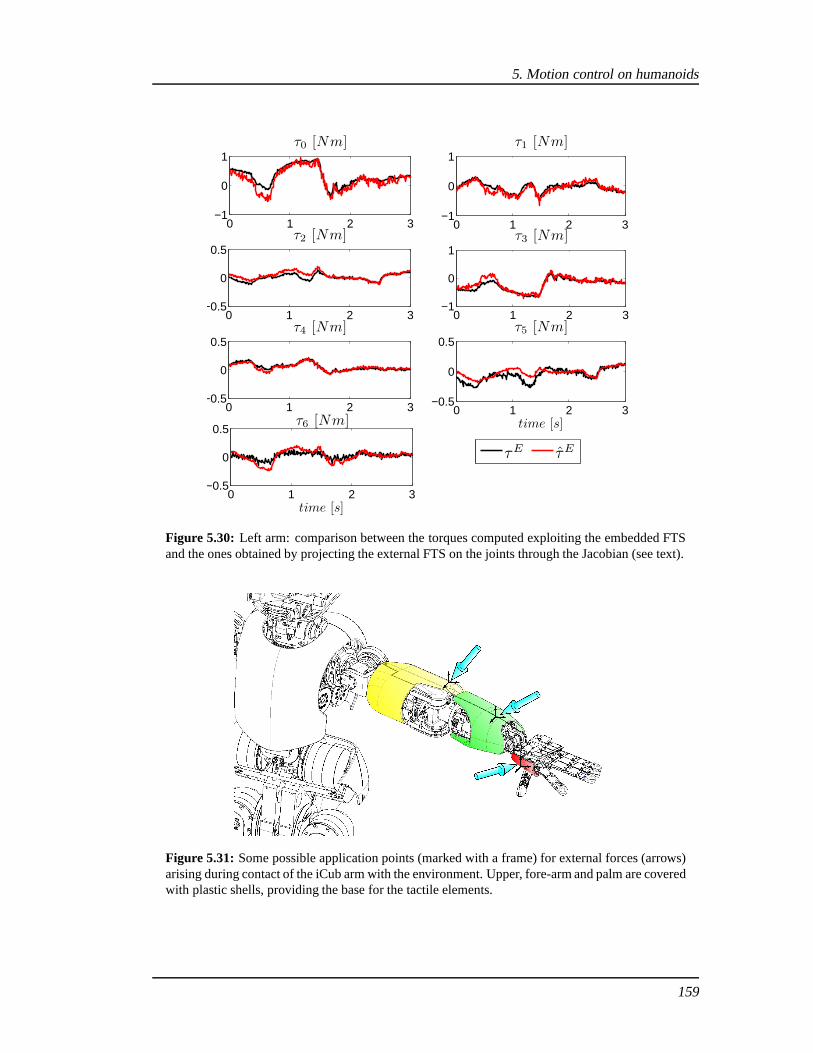
5. Motion control on humanoids
0 1 2 3−1
0
1τ0 [Nm]
0 1 2 3−1
0
1τ1 [Nm]
0 1 2 3−0.5
0
0.5τ2 [Nm]
0 1 2 3−1
0
1τ3 [Nm]
0 1 2 3−0.5
0
0.5τ4 [Nm]
0 1 2 3−0.5
0
0.5
time [s]
τ5 [Nm]
τE τE
0 1 2 3−0.5
0
0.5
time [s]
τ6 [Nm]
Figure 5.30: Left arm: comparison between the torques computed exploiting the embedded FTSand the ones obtained by projecting the external FTS on the joints through the Jacobian (see text).
Figure 5.31: Some possible application points (marked with a frame) for external forces (arrows)arising during contact of the iCub arm with the environment.Upper, fore-arm and palm are coveredwith plastic shells, providing the base for the tactile elements.
159

Figure 5.32:A sketch of the different situations in case of contacts occurring at different locations
in the left arm, as shown in Figure 5.31. The external wrench to estimate (◊) is attached to differentnodes. In the first and second sub-graphs, the wrench at the end-effector is assumed to be known(⧫), typically null, since only one unknown per graph is allowed (see text for details).
5.5.3 Joint impedance control of the iCub elbow
Robots with rigid joint, like iCub, can be controlled in torque by simply commanding a feed-forward torque, i.e.τff = τ . If robots are actuated by flexible joints, joint stiffness can be alsocontrolled. In iCub, actuation is provided by rigid electric motors, however a joint impedancecontrol interface is available, which can be exploited to emulate a compliant joint: in parti-cular, it is possible to control the equilibrium position ofa virtual spring and its stiffness anddamping. Precisely, the joint impedance control law is:
τ∗ = −kS (q − q∗) − kD q + τoffset (5.15)
wherekS , kD > 0 are the stiffness and damping constants, emulating a virtual spring at the joint,andτff a feed-forward offset torque. The desired computed torqueτ∗ is tracked at lower levelby a simple PID algorithm. Playing with stiffness and damping, it is possible to make the robotjoint behave like a soft or hard spring, while maintaining control on the desired joint position.Notably,kS andkD are physically related, as shown in Figure 5.33: the dampingconstant mustincrease with the stiffness, to prevent unstable behaviors. In the following experiment, we aimat demonstrating that by controlling a manipulator by suitably adapting stiffness and torque, ina feedforward manner, it is possible to cope with uncertainties and time delays in the system.
For sake of simplicity, we consider a single joint arm, moving in the vertical plane, de-scribed, as in Eq. 4.65, by the generic dynamic equation, which in the case of a single DOF canbe simply written as:
τ =m lC cos(q) g + (m l2 + I )q = G(q) +Bq (5.16)
whereτ is the joint torque,m, lC , I the link mass, length of the COM, and inertia respectively.
160
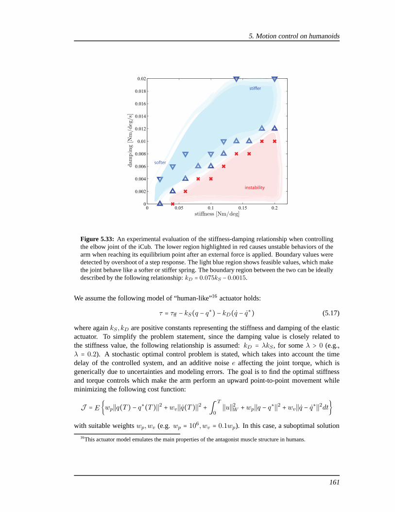
5. Motion control on humanoids
0 0.05 0.1 0.15 0.20
0.002
0.004
0.006
0.008
0.01
0.012
0.014
0.016
0.018
0.02
stiffness [Nm/deg]
dam
pin
g[N
m/d
eg/s
]
instability
softer
sti er
Figure 5.33: An experimental evaluation of the stiffness-damping relationship when controllingthe elbow joint of the iCub. The lower region highlighted in red causes unstable behaviors of thearm when reaching its equilibrium point after an external force is applied. Boundary values weredetected by overshoot of a step response. The light blue region shows feasible values, which makethe joint behave like a softer or stiffer spring. The boundary region between the two can be ideallydescribed by the following relationship:kD = 0.075kS − 0.0015.
We assume the following model of “human-like”16 actuator holds:
τ = τff − kS(q − q∗) − kD(q − q∗) (5.17)
where againkS , kD are positive constants representing the stiffness and damping of the elasticactuator. To simplify the problem statement, since the damping value is closely related tothe stiffness value, the following relationship is assumed: kD = λkS , for someλ > 0 (e.g.,λ = 0.2). A stochastic optimal control problem is stated, which takes into account the timedelay of the controlled system, and an additive noisee affecting the joint torque, which isgenerically due to uncertainties and modeling errors. The goal is to find the optimal stiffnessand torque controls which make the arm perform an upward point-to-point movement whileminimizing the following cost function:
J = E wp∣∣q(T ) − q∗(T )∣∣2 +wv ∣∣q(T )∣∣2 + ∫ T
0
∣∣u∣∣2W +wp∣∣q − q∗∣∣2 +wv ∣∣q − q∗∣∣2dtwith suitable weightswp,wv (e.g.wp = 106,wv = 0.1wp). In this case, a suboptimal solution
16This actuator model emulates the main properties of the antagonist muscle structure in humans.
161

0 50 100 150 20020
30
40
50
60
q[d
eg]
0 50 100 150 200−20
0
20
40
q[d
eg/s]
time instants
(a)
0 50 100 150 2000
0.02
0.04
0.06
0.08
ks
[Nm
/deg
]
0 50 100 150 2000
0.2
0.4
0.6
0.8
τ[N
m]
time instants
(b)
Figure 5.34: An experiment consisting of multiple trials, the iCub elbowfollows desired profiles(red) for stiffness and torque. Desired trajectories have been precomputed by the iLQG solving astochastic optimal control problem.5.34(a)joint position and velocity.5.34(b)joint stiffness andtorque.
has been found by means of the iLQG algorithm [Todorov and Li,2005].17 The following pa-rameters, compatible with the forearm of the iCub, were usedto describe the system dynamics:
• mass:m = 0.812kg• link length: a = 0.2735m• link COM: lC = 0.1033m• link inertia: I = 5.0826 × 10⁻³kg m2
The desired movement was set fromq∗0= −60 to q∗T = −30 degrees, which were remapped in
the iCub elbow joint range. The movement durationT was set to1.5s, while the control ratewas set to10ms. The additive noisee was modeled by:
e = (α + βq)η (5.18)
whereη has a normal distribution (η ≈ N(0,1)). Interestingly, the analysis has been performedon a further model, where the error is also proportional to the control torque:
e = (α + βq + γτ)η (5.19)
which accounts for a control-dependent noise. In order to set reasonable values of the pa-rameters, the modeling error has been identified: precisely, estimated joint torque has been
17The description of the iLQG method and its implementation isnot reported here, for not being completelyrelevant to the experiment discussion.
162

5. Motion control on humanoids
10 20 30 40 50−0.1
0
0.1
0.2
0.3
0.4
0.5
0.6
0.7
0.8
0.9
joint velocity [deg/s]
e[N
m]
joint torque error
stdmean
Figure 5.35: Mean e and standard deviationσe of the joint torque error from the elbow jointof iCub’s right arm. The standard deviation is evidently bilinear with the increase of velocity,while the error mean is linearly proportional to the velocity. Polynomial fitting models areσe =1.254q2 − 0.351q + 0.057 ande = 0.213q − 0.049 respectively.
compared with the one computed by (5.16), so thate = τmeasured − τmodel. A sequence of up-ward movements with a minimum jerk profile was performed withthe right arm of iCub, withincreasing average velocity (from0 to 55 deg/s): mean and standard deviations of the errorsare reported in Figure 5.35. Then, a normality test onη was performed, exploring within rea-sonable accuracy the parameter spaceα−β over a discrete grid in the range[0.0 ∶ 0.001 ∶ 1.0].Precisely, the Jarque-Bera test [Jarque and Bera, 1987] available in Matlab, was used. The bestsets of parameters found after the exploration were(α, β) = (0.15,0.37) for the model (5.18)and(α, β, γ) = (0.04,0.41,0.21) for (5.19): their fitting is shown in Figure 5.36.
Once the stochastic optimal control problem has been solved, the desired trajectories havebeen used to control the iCub elbow stiffness and torque, in afeedforward manner. To adaptthe computational control (5.17) to the robot available interface (5.15), the following has beendefined:τoffset = τff + kD q∗.
Preliminary results are shown in Figure 5.34. Some observations must be made. The damp-ing effect is evident, introducing a small but noticeable delay in the trajectory. The stiffnesstrajectory features extremely low values: however, the point of this experiment is to show thatthe feed-forward termτff is sufficient to achieve a desired behavior and that stiffness duringtrajectory must be increased only to counterbalance the uncertainties and noise in the problem.Thus, it is also correct to expect some misalignments between the desired and real trajectories.Moreover, there’s a known problem with the stiffness values: the resolution of the stiffness val-
163

ues in the DSP is0.01 Nm/deg, which is quite high for the trajectories we are aiming to: thismeans that the desired stiffness trajectory is practically“truncated” and actually is quantized.Another flaw in the experiments is that torques are estimatedby the EOG on the basis of themeasurements from the FTS, which have a certain drift duringthe use. This drift can be com-pensated, however it is not yet fully predictable. So it happens that a certain offset between themodel and the real measurements is affecting our results pertrial (for example, in the figures itis approximately0.1Nm): this explains the differences between the desired torque and the oneestimated (with a certain delay, again) by the robot dynamics module.
To overcome these issues, we are currently performing the same experiments on a prototypeof the new arm of the iCub, which is equipped with a joint torque sensor at the elbow.
164

5. Motion control on humanoids
0 200 400 600 800 1000 1200−3
−2
−1
0
1
2
3
time [ms]
torq
ue
erro
r[N
m]
e = (α + βq)η , α = 0.15, β = 0.37
eη
−4 −3 −2 −1 0 1 2 3 40
10
20
30
40
50
(a)
0 100 200 300 400 500 600 700 800 900 1000−3
−2
−1
0
1
2
3e = (α + βq + γτ )η , α = 0.04, β = 0.41, γ = 0.21
time [ms]
torq
ue
erro
r[N
m]
−4 −3 −2 −1 0 1 2 3 40
10
20
30
40
50
ηN(0,1)
(b)
Figure 5.36:An experimental evaluation of the elbow joint torque error due to uncertainties in thedynamic model of the iCub arm. Examples ofη (histogram) fitting a normal Gaussian (red line)are presented.5.36(a)shows the torque errore modeled by Eq. 5.18, while5.36(b)by Eq. 5.19.
165

166

Chapter 6
Conclusions
Optimal control theory has recently become of great interest for neuroscience, since it providesa framework and a rich set of tools for describing and modeling computational motor control ina convenient way. The existence of “optimality” principlesin sensori-motor control in the brainand in the CNS has been demonstrated in different experiments, focusing on the precomputa-tion of motor commands, trajectories, feedback and feed-forward commands. However, thereis not a unique answer to what mechanisms are really at the basis of our motions: a variety ofoptimal control models has been proposed, and since different models are apparently equallyeffective in explaining movements in the same or a similar context, it is difficult to assess whichis the most representative of human movements, and why.
Notably, by investigating human motor control it is not infrequent to address similar prob-lems as the ones engineers usually face in robotics, and especially in humanoid robotics. Byimplementing what we believe the optimality principles underlying the human CNS, it is pos-sible not only to provide an experimental verification of theproposed models, but also achievebehaviors which may outperform traditional classical controls. The point being that while clas-sical control theory has been mainly focused on minimizing tracking errors, reject disturbances,minimize the motion duration, guarantee stability, etc., the study of human motor control mayunveil other criteria as the fundamentals for achieving peculiar performances and characteris-tics which make our motor control so efficient and “optimal”,in a sense.
But, when trying to transfer human models on a robot, one faces several limits: in termsof physical and structural impairments in the architecture, in the technology for actuation andsensing, and in the theoretical tools which can be exploitedto generate controls. It is thencrucial to catch the biological principles of human motor controls and understand to whichextent these principles can be implemented in a robotic platform, and evaluate what is therevenue of that process. This thesis actually followed thispoint.
The first part of this thesis addressed the solution of stochastic optimal control problems,which can be used to state control problems to study both humans and humanoids, accordingto recent theories in computational motor control. The availability of powerful mathematicaltools for generating suitable controls is particularly crucial: indeed, classical control theoryis built on top of strong assumptions, as the known LQG conditions, which are hard to beverified in experimental platforms such as robots. With thisthesis, we propose a theoretical
167

tool which can be used to generate optimal controls for a wider class of problems, since itdoes not require particular features (neither in the systemnor in the cost functions) but thecontinuity and differentiability of their actors. Thus, itcan be applied to complex systems suchas humanoid without restricting assumptions. The applicability of the proposed approach hasbeen empirically demonstrated by several numerical and experimental examples, with linearand nonlinear systems.
However, there are several issues which still need to be addressed and remain open forfurther research. First, the convergence for the stochastic approximation algorithm cannot beguaranteed, and in general does not always occur. A certain practical experience with theoffline optimization is required. A possible solution to cutdrastically the time required to trainthe neural approximators would be to parallelize the computations and run the optimizationover a high-performance cluster grid of GPUs. This is not enough to guarantee to find theglobal optima of the control problem, however a considerable search in the parameter space canbe performed, even if not exhaustively, and to a certain extent it can help excluding unfeasiblecontrol laws. The time constraint is the main limitation of the proposed technique, since findinga solution (global or local) requires a considerable amountof training time and samples, thuslimiting the application domain of the technique to offline optimization. However, once theapproximating functions are trained, even in a rough manner, the algorithm is also suited foran incremental training which can be perfectly integrated on a modular robot architecture.
Despite its flaws, results obtained applying the method in different case studies are promis-ing: in particular, for the application in real-time domains such as robotics, since pre-computingthe control laws allows saving time during online execution. The performances of the RH neu-ral controller combined with the CLIK were impressive on James, and given the elasticity of theplatform were particularly positive. It is also worth noting that the experiments performed onJames were also the first (to the best of our knowledge) where the ERIM has been successfullyapplied for the control a real physical system.
Another interesting advantage of the proposed approach is that the formulation of the motorcontrol problem in the stochastic optimal control framework is particularly suited for findingcontrol laws in a modular architecture, where multiple agents coexist and in a sense cooperateto achieve the same goal. A brief hint of these future developments has been discussed inSection 3.3.4, where the main concepts of Team Theory have been introduced. Since the CAof the robot is basically a pool of modular controllers, interacting with each other regularly,it would be more than interesting to investigate a parallel between CNS and CA, and modelinterconnections between different controllers acting onthe robot: each may have its own goal,but they all cooperate for the same task accomplishment.
The second part of the thesis has been dedicated to the development of a theoretical frame-work which allows integrating dynamics in motor control models, providing both an estimateof the joint torques and a detection of external forces due tocontacts.
The estimation of the latter on the iCub has been particularly significant: it is clear that theproposed method is fundamental for enabling force/torque control in a platform where a directjoint torque feedback is missing. The main disadvantage of the FTS-based method is indeed thedelay caused by the software estimation of the torques, which cannot be done directly on theDSP but is performed on a remote machine. In this regard, we are currently investigating the
168
6. Conclusions
performances of the torque estimation via EOG on the prototype of the new iCub arm, whichwill be equipped with direct joint torque sensing.
However, numerous experiments in iCub involving active force control showed the effec-tiveness of the proposed approach, which has been already integrated in other modules of theiCub software library. The current implementation of the robot dynamics paves the way fornumerous developments: e.g., the integration of the dynamics computations with the tactilefeedback of the artificial skin, for accurate detection of external forces; the explicit computa-tion of the forward and inverse dynamics of the iCub limbs, toallow more advanced controlschemes; the accurate estimation of the dynamical parameters of the robot (since only CADparameters have been used so far).
The message emerging from the experimental results discussed in this thesis is that thereis more than a rationale in using the formalism of stochasticoptimal control to model humanmovements. The main benefit of such an abstract mathematicalframework is that the keyconcepts and motion criteria can be “ported” from humans to humanoids and vice versa ina relatively easy way, i.e. a parallel between the two systems can be done. Within certainlimitations, it is also possible to integrate successfullythe computational motor control modelsprovided by neuroscience into controllers for humanoid robots, which is particularly convenientsince the proposed optimal control framework is also suitedfor continuous adaptation andincremental learning, i.e. it can be combined with a developmental approach to humanoidrobotics.
169

170

Publications
Submitted / in preparation
1. S. Ivaldi, M. Fumagalli, M. Randazzo, F. Nori, G. Metta, G.Sandini. “Computing robotinternal/external wrenches by means of F/T sensors: theoryand implementation on theiCub humanoid.”
2. M. Fumagalli, S. Ivaldi, M. Randazzo, F. Nori, G. Metta, G.Sandini. “Force feedbackexploiting tactile and proximal force/torque sensing: theory and implementation on thehumanoid robot iCub”.
3. L. Natale, F. Nori, G. Metta, M. Fumagalli, S. Ivaldi, U. Pattacini, M. Randazzo, A.Schmitz and G. Sandini. “Studying developmental robotics on the iCub platform”.
4. B. Berret, S. Ivaldi, F. Nori, G. Sandini. “On the role of muscle co-contraction in plan-ning movements: implications on novel robotic actuators”.
≈≈≈Book chapters
1. M. Fumagalli, A. Gijsberts, S. Ivaldi, L. Jamone, G. Metta, L. Natale, F. Nori and G.Sandini. “Learning how to exploit proximal force sensing: acomparison approach”.O. Sigaud & J. Peters (eds.),From Motor Learning to Interaction Learning in Robots,Studies in Computational Intelligence, vol. 264, Springer-Verlag pp.159-177, 2010.
2. S. Ivaldi, M. Baglietto, G. Metta and R. Zoppoli. “An application of receding-horizonneural control in humanoid robotics”.Assessment and Future Directions of NonlinearModel Predictive Control, in L. Magni et al. (Eds.): Nonlinear Model Predictive Control,LNCIS 384, Springer-Verlag Berlin Heidelberg, pp. 541-550, 2009.
International Conference papers
1. S. Ivaldi, M. Fumagalli, F. Nori, M. Baglietto, G. Metta and G. Sandini. “Approximateoptimal control for reaching and trajectory planning in a humanoid robot”.Proc. of the2010 IEEE/RSJ International Conference on Intelligent Robots and Systems - IROS ’10.October 18-22 2010, Taipei, Taiwan.
171

2. S. Ivaldi, M. Baglietto, F. Davoli and R. Zoppoli. “Optimal control of communicationin energy constrained sensor networks through team theory and Extended RItz Method”.Proc. of the 2009 Int. Joint Conference on Neural Networks - IJCNN ’09, pp. 1372-1379.June 2009, Atlanta, GA, USA.
3. S. Ivaldi, M. Baglietto, G. Metta and R. Zoppoli. “An application of receding-horizonneural control in humanoid robotics”.Proc. Int. Workshop on current research andfuture directions of Nonlinear Model Predictive Control - NMPC ’08, pp. 1-8. September2008, Pavia, Italy.
4. S. Ivaldi, M. Baglietto and R. Zoppoli. “Finite and Receding Horizon Regulation of aSpace Robot”.Proc. Int. Conf. on Mathematical Problems in Engineering , Aerospaceand sciences - ICNPAA ’08, pp. 608-616. June 2008, Genoa, Italy.
Refereed short papers and presentations at International conferences
1. S. Ivaldi, A. Sciutti. “Aquabot”. “Affordable robots” idea context of the 2009 Int.Conf. on Advanced Robotics - ICAR ’09.June 2009, Munich, Germany. Third rank.(Project/presentation)
2. S. Ivaldi, A. Sciutti. “Night garbage collectobot”.“Affordable robots” idea context ofthe 2009 Int. Conf. on Advanced Robotics - ICAR ’09.June 2009, Munich, Germany.Accepted, but not selected for the final context. (Project/presentation)
3. S. Ivaldi, M. Baglietto, G. Metta, R. Zoppoli and G. Sandini. “A finite and receding hori-zon neural controller in humanoid robotics”.IEEE/RAS Int. Conference on IntelligentRobots and Systems - Workshop: Robotics challenges for machine learning II - IROS’08. September 2008, Nice, France. (Short paper and poster)
Refereed abstracts at National conferences
1. S. Ivaldi, M. Baglietto, F. Davoli and R. Zoppoli. “Extended Ritz Method for optimalcontrol of communication in energy constrained mixed (analog/digital) transmissions”.SIDRA annual conference ’09. September 2009, Siracusa, Italy. (Abstract and poster)
2. S. Ivaldi, M. Baglietto, G. Metta and R. Zoppoli. “An application of receding horizonneural control in humanoid robotics”.SIDRA annual conference ’08. September 2008,Vicenza, Italy. (Abstract and talk)
3. S. Ivaldi, M. Baglietto, R. Zoppoli. “Extended Ritz Method for optimal control in com-munication problems”.SIDRA Annual Conference ’07. September 2007, Genoa, Italy.(Abstract and poster)
172

Bibliography
[Aicardi et al., 1995] Aicardi, M., Casalino, G., Bicchi, A., and Balestrino, A. (1995). Closedloop steering of unicycle like vehicles via lyapunov techniques.IEEE Robotics AutomationMagazine, 2(1):27–35.
[Albers, 2002] Albers, A. (2002). Conceptual design of humanoid robots. InThe Third IARPInternational Workshop on Humanoid and Human Friendly Robotics, Tsukuba ResearchCenter, AIST, Tsukuba, Ibaraki, Japan.
[Albu-Schaffer et al., 2010] Albu-Schaffer, A., Wolf, S., Eiberger, O., Haddadin, S., Petit, F.,and Chalon, M. (2010). Dynamic modelling and control of variable stiffness actuators. InIEEE Int. Conf. on Robotics and Automation, pages 2155–2162, Anchorage, Alaska, USA.
[Amundson et al., 2005] Amundson, K., Raade, J., Harding, N., and Kazerooni, H. (2005).Hybrid hydraulic-electric power unit for field and service robots. InIEEE/RSJ Int Conf. onIntelligent Robots and Systems.
[Arechavaleta et al., 2008] Arechavaleta, G., Laumond, J.,Hicheur, H., and Berthoz, A.(2008). An optimality principle governing human walking.IEEE Transactions on Robotics,24:5–14.
[ATI, www] ATI (www). http://www.ati-ia.com/products/ft/ft models.aspx?id=mini45.
[Atkenson and Whitman, 2009] Atkenson, C. and Whitman, E. (2009). Dynamic program-ming approaches to humanoid behavior optimization. InIEEE-RAS Humanoids 09 - Work-shop: Modeling, Simulation and Optimization of Bipedal Walking, Paris, France.
[Atkeson and Stephens, 2007] Atkeson, C. and Stephens, B. (2007). Multiple balance strate-gies from one optimization criterion. InIEEE Int. Conf. on Humanoid Robots.
[Atkeson et al., 2000] Atkeson, C. G., Hale, J. G., Pollick, F., Riley, M., Kotosaka, S., Schaul,S., Shibata, T., Tevatia, G., Ude, A., Vijayakumar, S., Kawato, E., and Kawato, M. (2000).Using humanoid robots to study human behavior.IEEE Intelligent Systems and Their Ap-plications, 15(4):46–56.
[Baglietto, 1998] Baglietto, M. (1998).Nonlinear Approximators for Team Optimal ControlProblems. PhD thesis, University of Genova.
173

[Baglietto et al., 2001a] Baglietto, M., Parisini, T., and Zoppoli, R. (2001a). The case of dy-namic routing in traffic networks.IEEE Transactions on Neural Networks, 12:485–502.2004 IEEE Transactions on Neural Networks Outstanding Paper Award.
[Baglietto et al., 2001b] Baglietto, M., Parisini, T., and Zoppoli, R. (2001b). Numerical solu-tions to the witsenhausen counterexample by approximatingnetworks. IEEE Transactionson Automatic Control, 46(9):1471–1477.
[Barambones and Etxebarria, 2002] Barambones, O. and Etxebarria, V. (2002). Robust neuralcontrol for robotic manipulators.Automatica, 38:235 – 242.
[Barron, 1993] Barron, A. R. (1993). Universal approximation bounds for superpositions of asigmoidal function.IEEE Transactions on Information Theory, 39(3):930 – 945.
[Barron, 1994] Barron, A. R. (1994). Approximation and estimation bounds for artificial neu-ral networks.Machine Learning, 14:115 – 133.
[Bauml et al., 2010] Bauml, B., Wimbock, T., and Hirzinger, G. (2010). Kinematically opti-mal catching a flying ball with a hand-arm-system. InIEEE/RSJ Int. Conf. on IntelligentRobots and Systems, pages 2592–2599, Taipei, Taiwan.
[Beamish et al., 2006] Beamish, D., Bhatti, S. A., MacKenzie, I. S., and Wu, J. (2006). Fiftyyears later: A neurodynamic explanation of fitts’ law.J R Soc Interface, 3(10):649–654.
[Bellman, 1957] Bellman, R. (1957).Dynamic Programming. Princeton Univeristy Press,Princeton, NJ.
[Ben-Itzhak and Karniel, 2008] Ben-Itzhak, S. and Karniel,A. (2008). Minimum accelerationcriterion with constraints implies bang-bang control as anunderlying principle for optimaltrajectories of arm reaching movements.Neural Computation, 20(3):779–812.
[Bennequin et al., 2009] Bennequin, D., Fuchs, R., Berthoz,A., and Flash, T. (2009). Move-ment timing and invariance arise from several geometries.PLoS Computational Biology,5(7):e1000426.
[Berret et al., 2008] Berret, B., Darlot, C., Jean, F., Pozzo, T., Papaxanthis, C., and Gauthier,J. (2008). The inactivation principle: mathematical solutions minimizing the absolute workand biological implications for the planning of arm movements. PLoS Computational Biol-ogy, 4(10):e1000194.
[Bertsekas and Tsitsiklis, 1996] Bertsekas, D. and Tsitsiklis, J. (1996). Neuro-dynamic pro-gramming. Athena.
[Bertsekas, 1995] Bertsekas, D. P. (1995).Dynamic Programming and Optimal Control.Athena Scientific.
[Biess et al., 2007] Biess, A., Liebermann, D. G., and Flash,T. (2007). A computational modelfor redundant human three-dimensional pointing movements: integration of independent
174

BIBLIOGRAPHY
spatial and temporal motor plans simplifies movement dynamics. The Journal of Neuro-science, 27(48):13045–13064.
[Biess et al., 2006] Biess, A., Nagurka, M., and Flash, T. (2006). Simulating discrete andrhythmic multi-joint human arm movements by optimization of nonlinear performance in-dices.Biological Cybernetics, 95(1):31–53.
[Blair and Iwasaki, 2011] Blair, J. and Iwasaki, T. (2011). Optimal gaits for mechanical recti-fier systems.Automatic Control, IEEE Transactions on, 56(1):59–71.
[Braganza et al., 2005] Braganza, D., W.E.Dixon, Dawson, D., and Xian, B. (2005). Trackingcontrol for robot manipulators with kinematic and dynamic uncertainty. InProc. of the 44thIEEE Conference on Decision and Control, and the European Control Conference 2005.
[Braun et al., 2009] Braun, D., Aertsen, A., Wolpert, D., andMehring, C. (2009). Learningoptimal adaptation strategies in unpredictable motor tasks. The Journal of Neuroscience,29(20):6472–6478.
[Brock et al., 2008] Brock, O., Kuffner, J., and Xiao, J. (2008). Springer Handbook ofRobotics, chapter Motion for manipulation tasks, pages 615–645. Siciliano, Khatib (Eds.),Springer.
[Caccavale et al., 2005] Caccavale, F., Natale, C., Siciliano, B., and Villani, L. (2005). Integra-tion for the next generation: embedding force control into industrial robots.IEEE RoboticsAutomation Magazine, 12(3):53–64.
[Calinon et al., 2010] Calinon, S., Sardellitti, I., and Caldwell, D. (2010). Learning-basedcontrol strategy for safe human-robot interaction exploiting task and robot redundancies. InIEEE/RSJ Int. Conf. on Intelligent Robots and Systems, Taipei, Taiwan.
[Cannata et al., 2008] Cannata, G., Maggiali, M., Metta, G.,and Sandini, G. (2008). An em-bedded artificial skin for humanoid robots. InIEEE Int. Conf. on Multisensor Fusion andIntegration, Seoul, Korea.
[Cawley, 2006] Cawley, G. C. (2006). Leave-one-out cross-validation based model selectioncriteria for weighted ls-svms. InIJCNN-2006: Proceedings of the International Joint Con-ference on Neural Networks, pages 1661–1668, Vancouver, BC, Canada.
[Chevallereau and Aoustin, 2001] Chevallereau, C. and Aoustin, Y. (2001). Optimal referencetrajectories for walking and running of a biped robot.Robotica, 19:557–569.
[Chiaverini et al., 1991] Chiaverini, S., Egeland, O., and Kanestrom, R. K. (1991). Achievinguser-defined accuracy with damped least-squares inverse kinematics. InProc. Fifth Interna-tional Conference on Advanced Robotics ’Robots in Unstructured Environments’, 91 ICAR,pages 672–677.
[Chiaverini et al., 2008] Chiaverini, S., Oriolo, G., and Walker, I. (2008). Springer Hand-book of Robotics, chapter Kinematically redundant manipulators, pages 245–268. Siciliano,Khatib (Eds.), Springer.
175

[Chiaverini et al., 1999] Chiaverini, S., Siciliano, B., and Villani, L. (1999). A survey of robotinteraction control schemes with experimental comparison. Mechatronics, IEEE/ASMETransactions on, 4(3):273 –285.
[Cormen et al., 2002] Cormen, T., Leiserson, C., Rivest, R.,and Stein, C. (2002).Introductionto Algorithms. McGraw-Hill Higher Education, 2 edition.
[De Luca, 2006] De Luca, A. (2006). Collision detection and safe reaction with the dlr-iiilightweight manipulator arm. InIEEE/RSJ Int. Conf. on Intelligent Robots and Systems,pages 1623–1630.
[Degallier et al., 2008] Degallier, S., Righetti, L., Natale, L., Nori, F., Metta, G., and Ijspeert,A. (2008). A modular bio-inspired architecture for movement generation for the infant-likerobot icub. InIEEE RAS / EMBS Int. Conf. on Biomedical Robotics and Biomechatronics,Scottsdale, Arizona.
[Denavit and Hartenberg, 1955] Denavit, J. and Hartenberg,R. S. (1955). A kinematic nota-tion for lower-pair mechanisms based on matrices.Journal of Applied Mechanics, 23:215–221.
[Diedrichsen et al., 2010] Diedrichsen, J., Shadmehr, R., and Ivry, R. (2010). The coordinationof movement: optimal feedback control and beyond.Trends in Cognitive Science, 14:1.
[Diehl et al., 2006] Diehl, M., Bock, H., Diedam, H., and Wieber, P. (2006).Fast Motions inBiomechanics and Robotics, chapter Fast Direct Multiple Shooting algorithms for optimalrobot control, pages 65–93. LNCIS 340, Springer Berlin / Heidelberg.
[Diehl et al., 2009] Diehl, M., Ferreau, H., and Haverbeke, N. (2009). L. Magni et al. (Eds.):Nonlinear Model Predictive Control, chapter Efficient numerical methods for nonlinearMPC and Moving Horizon estimation, pages 541–550. LNCIS 384, Springer-Verlag BerlinHeidelberg.
[Duda et al., 2001] Duda, R. O., Hart, P. E., and Stork, D. G. (2001). Pattern Classification.Wiley-Interscience.
[Dupree et al., 2009] Dupree, K., Patre, P., Johnson, M., andDixon, W. (2009). Inverse opti-mal adaptive control of a nonlinear euler-lagrange system,part i: Full state feedback. In48thIEEE Conf. on Decision and Control, held jointly with 28th Chinese Control Conference.CDC/CCC 2009, pages 321–326.
[Eiberger et al., 2010] Eiberger, O., Haddadin, S., Weis, M., Albu-Schaffer, A., and Hirzinger,G. (2010). On joint design with intrinsic variable compliance: derivation of the DLR QA-joint. In IEEE Int. Conf. on Robotics and Automation, pages 1687–1694.
[Faulhaber, www] Faulhaber (www). www.faulhaber.com.
[Featherstone, 2007] Featherstone, R. (2007).Rigid Body Dynamics Algorithms. Springer-Verlag New York, Inc., Secaucus, NJ, USA.
176

BIBLIOGRAPHY
[Featherstone, 2010] Featherstone, R. (2010). Exploitingsparsity in operational-space dynam-ics. International Journal of Robotics Research, 29:1353–1368.
[Featherstone and Orin, 2008] Featherstone, R. and Orin, D.E. (2008).Handbook of Robotics,chapter Dynamics, pages 35–65. Springer.
[Fitts, 1954] Fitts, P. (1954). The information capacity ofthe human motor system in control-ling the amplitude of movement.J. Exp. Psychol., 47(6):381–391.
[Fitzpatrick et al., 2008] Fitzpatrick, P., Metta, G., and Natale, L. (2008). Towards long-livedrobot genes.Robotics and Autonomous Systems, 56:29–45.
[Fitzpatrick et al., 2010] Fitzpatrick, P., Natale, L., andMetta, G. (2010). The Cmaking of ahumanoid.The Kitware Source: Software Developer’s Quarterly, 13:7–9.
[Flanagan et al., 2003] Flanagan, J., Vetter, P., Johansson, R., and Wolpert, D. (2003). Predic-tion precedes control in motor learning.Current Biology, 13:146–150.
[Flash and Hogan, 1985] Flash, T. and Hogan, N. (1985). The coordination of arm move-ments: an experimentally confirmed mathematical model.The Journal of Neuroscience,5(7):1688–1703.
[Franklin et al., 2008] Franklin, D., Burdet, E., Tee, K., Osu, R., Chew, C.-M., Milner, T., andKawato, M. (2008). Cns learns stable, accurate, and efficient movements using a simplealgorithm.The Journal of Neuroscience, 28(44):11165–11173.
[Freescale DSP, www] Freescale DSP (www). http://www.freescale.com/.
[Fumagalli et al., 2010a] Fumagalli, M., Gijsberts, A., Ivaldi, S., Jamone, L., Metta, G., Na-tale, L., Nori, F., and Sandini, G. (2010a).O. Sigaud et al. (Eds.): From Motor Learningto Interaction Learning in Robots, chapter Learning to Exploit Proximal Force Sensing: aComparison Approach. Springer-Verlag.
[Fumagalli et al., 2009] Fumagalli, M., Jamone, L., Metta, G., Natale, L., Nori, F.,Parmiggiani, A., Randazzo, M., and Sandini, G. (2009). A force sensor for the controlof a human-like tendon driven neck. InIEEE-RAS International Conference on HumanoidRobots.
[Fumagalli et al., 2010b] Fumagalli, M., Randazzo, M., Nori, F., Natale, L., Metta, G., andSandini, G. (2010b). Exploiting proximal F/T measurementsfor the iCub active compliance.In IEEE/RSJ Int. Conf. on Intelligent Robots and Systems, Taipei, Taiwan.
[Gori and Tesi, 1992] Gori, M. and Tesi, A. (1992). On the problem of local minima in back-propagation.Pattern Analysis and Machine Intelligence, IEEE Transactions on, 14(1):76–86.
[Gu and Hu, 2005] Gu, D. and Hu, H. (2005). A stabilizing receding horizon regulator fornonholonomic mobile robots.IEEE Transactions on Robotics, 21:1022–1028.
177
[Guigon et al., 2008] Guigon, E., Baraduc, P., and Desmurget, M. (2008). Optimality, stochas-ticity and variability in motor behavior.Journ. Computational Neuroscience, 24(1):57–68.
[Haddadin et al., 2008a] Haddadin, S., Albu-Schaffer, A., ,and Hirzinger, G. (2008a). Therole of the robot mass and velocity in physical human-robot interaction - part i: Non-constrained blunt impacts. InIEEE Int. Conf. on Robotics and Automation, Pasadena, CA,USA.
[Haddadin et al., 2010a] Haddadin, S., Albu-Schaffer, A., Eiberger, O., and Hirzinger, G.(2010a). New insights concerning intrinsic joint elasticity for safety. InIEEE/RSJ Int.Conf. on Intelligent Robots and Systems.
[Haddadin et al., 2008b] Haddadin, S., Albu-Schaffer, A., Frommberger, M., , and Hirzinger,G. (2008b). The role of the robot mass and velocity in physical human-robot interaction- part ii: Constrained blunt impacts. InIEEE Int. Conf. on Robotics and Automation,Pasadena, CA, USA.
[Haddadin et al., 2010b] Haddadin, S., Urbanek, H., Parusel, S., Burschka, D., Rossmann, J.,Albu-Schaffer, A., and Hirzinger, G. (2010b). Real-time reactive motion generation basedon variable attractor dynamics and shaped velocities. InIEEE/RSJ Int. Conf. on IntelligentRobots and Systems, pages 3109 –3116.
[Hagan and Menhaj, 1994] Hagan, M. T. and Menhaj, M. B. (1994). Training feedforwardnetworks with the marquardt algorithm.IEEE Transactions on Neural Networks, 5(6):989–993.
[Harris and Wolpert, 1998] Harris, C. M. and Wolpert, D. M. (1998). Signal-dependent noisedetermines motor planning.Nature, 394(6695):780–784.
[He and Geng, 2007] He, G.-P. and Geng, Z.-Y. (2007). Optimalmotion planning of a one-legged hopping robot. InIEEE Int.Conf. on Robotics and Biomimetics, pages 1178–1183,Sanya, China.
[Hersch and Billard, 2006] Hersch, M. and Billard, A. (2006). A biologically-inspired con-troller for reaching movements. InBiomedical Robotics and Biomechatronics, 2006. BioRob2006. The First IEEE/RAS-EMBS International Conference on, pages 1067–1072.
[Ho and Chu, 1972] Ho, Y. and Chu, K. (1972). Team decision theory and information struc-tures in optimal control problems - part i.IEEE Transactions on Automatic Control, 17:15–28.
[Hornik et al., 1989] Hornik, K., Stinchombe, M., and White,H. (1989). Multilayer feedfor-ward networks are universal approximators.Neural Networks, 2(5):359–366.
[Ivaldi et al., 2009a] Ivaldi, S., Baglietto, M., Davoli, F., and Zoppoli, R. (2009a). Optimalcontrol of communication in energy constrained sensor networks through team theory andextended ritz method. InInt. Joint Conf. on Neural Networks, pages 1372–1379, Atlanta,GA, USA.
178

BIBLIOGRAPHY
[Ivaldi et al., 2008a] Ivaldi, S., Baglietto, M., Metta, G.,and Zoppoli, R. (2008a). An ap-plication of receding-horizon neural control in humanoid robotics. InInt. Workshop onAssessment and future directions of Nonlinear Model Predictive Control, Pavia, Italy.
[Ivaldi et al., 2009b] Ivaldi, S., Baglietto, M., Metta, G.,and Zoppoli, R. (2009b).L. Magniet al. (Eds.): Nonlinear Model Predictive Control. TowardsNew Challenging Applications,chapter An application of receding-horizon neural controlin humanoid robotics, pages 541–550. LNCIS 384, Springer-Verlag Berlin Heidelberg.
[Ivaldi et al., 2008b] Ivaldi, S., Baglietto, M., Metta, G.,Zoppoli, R., and Sandini, G. (2008b).A finite and receding horizon neural controller in humanoid robotics. In Int. Conf. OnIntelligent Robots - IROS. Workshop: Robotics Challenges for Machine Learning II.
[Ivaldi et al., 2008c] Ivaldi, S., Baglietto, M., and Zoppoli, R. (2008c). Finite and recedinghorizon regulation of a space robot. InInt. Conf. on Mathem. Probl. in Engin. Aerospaceand Sciences, pages 608–616. Cambridge Scientific Publishers, London.
[Ivaldi et al., 2010] Ivaldi, S., Fumagalli, M., Nori, F., Baglietto, M., and Metta, G. (2010).Approximate optimal control for reaching and trajectory planning in a humanoid robot. InIEEE/RSJ Int. Conf. on Intelligent Robots and Systems, pages 1290–1296, Taipei, Taiwan.
[Ivaldi et al., www] Ivaldi, S., Fumagalli, M., and Pattacini,U. (www). Doxygen documentation of the iDyn library.http://eris.liralab.it/iCub/main/dox/html/group__iDyn.html.
[Izawa et al., 2008] Izawa, J., Rane, T., Donchin, O., and Shadmehr, R. (2008). Motor adapta-tion as a process of reoptimization.The Journal of Neuroscience, 28(11):2883–2891.
[Jamone, 2010] Jamone, L. (2010).Autonomous sensori-motor learning in a humanoid robot.PhD thesis, University of Genoa, Italy.
[Jamone et al., 2006] Jamone, L., Metta, G., Nori, F., and Sandini, G. (2006). James: A hu-manoid robot acting over an unstructured world. InProc. 6th IEEE-RAS International Con-ference on Humanoid Robots, pages 143–150.
[Janabi-Sharifi et al., 2000] Janabi-Sharifi, F., Hayward, V., and Chen, C.-S. J. (2000).Discrete-time adaptive windowing for velocity estimation. IEEE Transactions on ControlSystems Technology, 8(6):1003–1009.
[Jarque and Bera, 1987] Jarque, C. and Bera, A. (1987). A testfor normality of observationsand regression residuals.International Statistical Review, 55(2):163–172.
[Kaneko et al., 2005] Kaneko, Y., Nakano, E., Osu, R., Wada, Y., and Kawato, M. (2005).Trajectory formation based on the minimum commanded torquechange model using euler-poisson equation.Systems and Computers in Japan, 36:92–103.
[Kanoun et al., 2009] Kanoun, O., Yoshida, E., and Laumond, J. (2009). An optimizationformulation for footsteps planning. InIEEE-RAS Int. Conf. on Humanoid Robots, pages202–207, Paris, France.
179

[Keerthi and Gilbert, 1988] Keerthi, S. and Gilbert, E. (1988). Optimal infinite-horizon feed-back laws for a general class of constrained discrete-time systems: stability and moving-horizon approximations.Journal of Optimization Theory and Applications, 57:265–293.
[Kelso, 1982] Kelso, J., editor (1982).Human motor behavior: an introduction. LawrenceErlbaum Associates Inc.
[Kim et al., 2000] Kim, Y. H., Lewis, F. L., and Dawson, D. M. (2000). Intelligent optimalcontrol of robotic manipulators using neural networks.Automatica, 36:1355 – 1364.
[Konczak and Dichgans, 1997] Konczak, J. and Dichgans, J. (1997). The development towardstereotypic arm kinematics during reaching in the first 3 years of life. Experimental BrainResearch, 117:346–354.
[Konczak et al., 2010] Konczak, J., Pierscianek, D., Hirsiger, S., Bultmann, U., Schoch, B.,Gizewski, E., Timmann, D., Maschke, M., and Frings, M. (2010). Recovery of upper limbfunction after cerebellar stroke: Lesion symptom mapping.Stroke, 41:2191–2200.
[Kozlowski, 1998] Kozlowski, K. (1998).Modelling and Identification in Robotics. Springer-Verlag New York, Inc., Secaucus, NJ, USA.
[Krstic, 2009] Krstic, M. (2009). Inverse optimal adaptivecontrol : the interplay betweenupdate laws, control laws, and lyapunov functions. InAmerican Control Conference, pages1250–1255.
[Krurkova, 1997] Krurkova, V. (1997).Dimension-independent rates of approximation byneural networks, pages 261–270. “Computer-intensive methods in control and signal pro-cessing: curse of dimensionality”. Warwick and Karny Eds.,Boston.
[Kulic and Croft, 2007] Kulic, D. and Croft, E. (2007). Pre-collision safety strategies forhuman-robot interaction.Autonomous Robots, 22:149–164.
[Kuo, 2005] Kuo, A. (2005). An optimal state estimation model of sensory integration inhuman postural balance.Journal of Neural Engineering, 2:S235–S249.
[Kurkova and Sanguineti, 2005] Kurkova, V. and Sanguineti, M. (2005). Error estimates forapproximate optimization by the extended ritz method.SIAM J. on optimization, 15:461–487.
[Kusher and Yin, 1997] Kusher, H. J. and Yin, G. G. (1997).Stochastic approximation algo-rithms and applications. Springer-Verlag, New York.
[Kushner and Yang, 1995] Kushner, H. and Yang, J. (1995). Stochastic approximation withaveraging and feedback: rapidly convergent “on-line” algorithms. IEEE Transactions onAutomatic Control, 40:24–34.
[Kwon et al., 1983] Kwon, W., Bruckstein, A., and Kailath, T.(1983). Stabilizing state-feedback design via the moving horizon method.International Journal of Control, 37:631–643.
180

BIBLIOGRAPHY
[Kwon and Han, 2005] Kwon, W. and Han, S. (2005).Receding horizon control: Model Pre-dictive Control for State Models. Springer-Verlag. Advanced Textbooks in Control andSignal processing. London, UK.
[Kwon and Paearson, 1978] Kwon, W. and Paearson, A. (1978). On feedback stabilization oftime-varying discrete linear systems.IEEE Transactions on Automatic Control, 23(3):479–481.
[Lacquaniti et al., 1983] Lacquaniti, F., Terzuolo, C., andViviani, P. (1983). The law relatingkinematic and figural aspects of drawing movements.Acta Psychologica, 54:115–130.
[Lagarde et al., 2009] Lagarde, M., Andry, P., Gaussier, P.,Boucenna, S., and Hafemeister, L.(2009). Proprioception and imitation: on the road to agent individuation. InFrom Motor toInteraction Learning in Robots. Springer.
[Lengagne et al., 2009] Lengagne, S., Ramdani, N., and Fraisse, P. (2009). Planning and fastre-planning of safe motions for humanoid robots: Application to a kicking motion. InIEEE/RSJ International Conference on Intelligent Robots and Systems, pages 441–446, St.Louis, US.
[Levenberg, 1944] Levenberg, K. (1944). A method for the solution of certain problems inleast squares.Quarterly of Applied Mathematics, 2:164–168.
[Lockhart and Ting, 2007] Lockhart, D. and Ting, L. (2007). Optimal sensorimotor transfor-mations for balance.Nature Neuroscience, 10(10):1329–1336.
[Luh et al., 1983] Luh, J., Fisher, W., and Paul, R. (1983). Joint torque control by a directfeedback for industrial robots.IEEE Trans. on Automatic Control, 28(2):153–161.
[MacKenzie, 1992] MacKenzie, I. (1992). Fitts’ law as a research and design tool in human-computer interaction.Human-Computer Interaction, 7:91–139.
[Maggiali et al., 2008] Maggiali, M., Cannata, G., Maiolino, P., Metta, G., Randazzo, M., andSandini, G. (2008). Embedded distributed capacitive tactile sensor. InMechatronics 2008,Limerick, Ireland.
[Mandersloot et al., 2006] Mandersloot, T., Wisse, M., and Atkeson, C. (2006). Controllingvelocity in bipedal walking: A dynamic programming approach. In6th IEEE-RAS Int. Conf.on Humanoid Robots, pages 124–130.
[Marquardt, 1963] Marquardt, D. (1963). An algorithm for least-squares estimation of nonlin-ear parameters.SIAM Journal on Applied Mathematics, 11:431–441.
[Matsui, 2008] Matsui, T. (2008). A new optimal control model for reproducing two-pointreaching movements of human three-joint arm with wrist joint’s freezing mechanism. InIEEE Int. Conf. on Robotics and Biomimetics, pages 383–388.
181
[Matsui et al., 2006] Matsui, T., Honda, M., and Nakazawa, N.(2006). A new optimal controlmodel for reproducing human arm’s two-point reaching movements: a modified minimumtorque change model. InIEEE Int. Conf. on Robotics and Biomimetics, pages 1541–1546.
[Matsui et al., 2009] Matsui, T., Takeshita, K., and Shibusawa, T. (2009). Effectiveness of hu-man three-joint arm’s optimal control model characterizedby hand-joint’s freezing mech-anism in reproducing constrained reaching movement characteristics. InICROS-SICE Int.Joint Conf. (ICCAS-SICE), pages 1206 –1211.
[Mayne and Michalska, 1990] Mayne, D. and Michalska, H. (1990). Receding horizon controlof nonlinear systems.IEEE Transactions on Automatic Control, 38(11):1623–1633.
[Metta et al., 2006] Metta, G., Fitzpatrick, P., and Natale,L. (2006). Yarp: yet another robotplatform. International Journal on Advanced Robotics Systems. Special Issue on SoftwareDevelopment and Integration in Robotics, 1(8/9):975–997.
[Metta et al., 2010] Metta, G., Natale, L., Nori, F., Sandini, G., Vernon, D., Fadiga, L., vonHofsten, C., Rosander, K., Santos-Victor, J., Bernardino,A., and Montesano, L. (2010).The icub humanoid robot: An open-systems platform for research in cognitive development.Neural Networks, special issue on Social Cognition: From Babies to Robots, 23:1125–1134.
[Metta et al., 1999] Metta, G., Sandini, G., and Konczak, J. (1999). A developmental approachto visually-guided reaching in artificial systems.Neural Networks, 12(10):1413–1427.
[Mettin et al., 2010] Mettin, U., Shiriaev, A., Freidovich,L., and Sampei, M. (2010). Optimalball pitching with an underactuated model of a human arm. InIEEE Int. Conf. on Roboticsand Automation, Anchorage, Alaska, USA.
[Michalska and Mayne, 1993] Michalska, H. and Mayne, D. (1993). Robust receding horizoncontrol of constrained nonlinear systems.IEEE Trans. on Automatic Control, 38:1623–1633.
[Minguez et al., 2008] Minguez, J., Lamiraux, F., and Laumond, J.-P. (2008).Handbook ofRobotics, chapter Motion planning and obstacle avoidance, pages 827–852. Springer.
[Mistry et al., 2008] Mistry, M., A.Theodorou, E., Liaw, G.,Yoshioka, T., Schaal, S., andKawato, M. (2008). Adaptation to a sub-optimal desired trajectory. InSociety for Neuro-science - Symposium on Advances in Computational Motor Control, Washington DC, USA.
[Mistry et al., 2010] Mistry, M., Buchli, J., and Schaal, S. (2010). Inverse dynamics control offloating base systems using orthogonal decomposition. InIEEE Int. Conf. on Robotics andAutomation.
[Mitrovic et al., 2010] Mitrovic, D., Klanke, S., and Vijayakumar, S. (2010).O. Sigaud, J.Peters (Eds.): From Motor to Interaction Learning in Robotics, chapter Adaptive OptimalFeedback Control with Learned Internal Dynamics Models, pages 65–84. SCI 264 Springer-Verlag Berlin Heidelberg.
182
BIBLIOGRAPHY
[Mombaur et al., 2008] Mombaur, K., Laumond, J.-P., and Yoshida, E. (2008). An optimalcontrol model unifying holonomic and nonholonomic walking. In 8th IEEE-RAS Int. Conf.on Humanoid Robots, Daejeon, Korea.
[Mombaur et al., 2010] Mombaur, K., Truong, A., and Laumond,J.-P. (2010). From humanto humanoid locomotionan inverse optimal control approach. Autonomous Robots, 28:369–383.
[Morasso, 1983] Morasso, P. (1983). Three dimensional arm trajectories.Biological Cyber-netics, 48:187–194.
[Morel and Dubowsky, 1996] Morel, G. and Dubowsky, S. (1996). The precise control ofmanipulators with joint friction: A base force/torque sensor method. InIEEE Int. Conf. onRobotics and Automation, pages 360–365.
[Morel et al., 2000] Morel, G., Iagnemma, K., and Dubowsky, S. (2000). The precise con-trol of manipulators with high joint friction using base force/torque sensing.Automatica,36(7):931–941.
[Murray et al., 1994] Murray, R. M., Sastry, S. S., and Zexiang, L. (1994). A MathematicalIntroduction to Robotic Manipulation. CRC Press, Inc., Boca Raton, FL, USA.
[Nagengast et al., 2011] Nagengast, A., Braun, D., and Wolpert, D. (2011). Risk-sensitivityand the mean-variance trade-off: decision making in sensorimotor control. Proceedings ofThe Royal Society B, doi: 10.1098/rspb.2010.2518:1–8.
[Nakano et al., 1999] Nakano, E., Imamizu, H., Osu, R., Uno, Y., Gomi, H., Yoshioka, T., andKawato, M. (1999). Quantitative examinations of internal representations for arm trajec-tory planning: Minimum commanded torque change model.Journal of Neurophysiology,81:2140–2155.
[Nelson, 1983] Nelson, W. (1983). Physical principles for economies of skilled movements.Biological Cybernetics, 46:135–147.
[Nguyen and Widrow, 1990] Nguyen, D. and Widrow, B. (1990). Improving the learningspeed of 2-layer neural networks by choosing initial valuesof the adaptive weights. InIJCNN International Joint Conference on Neural Networks, volume 3, pages 21–26, SanDiego, CA, USA.
[Niyogi and Girosi, 1996] Niyogi, P. and Girosi, F. (1996). On the relationship between gen-eralization error, hypothesis complexity, and sample complexity for radial basis functions.Neural Computation, 8:819 – 842.
[Nori et al., 2007a] Nori, F., Jamone, L., Sandini, G., and Metta, G. (2007a). Accurate controlof a human-like tendon-driven neck. InProc. 7th IEEE-RAS International Conference onHumanoid Robots, pages 371–378.
183

[Nori et al., 2007b] Nori, F., Natale, L., Sandini, G., and Metta, G. (2007b). Autonomouslearning of 3d reaching in a humanoid robot. InIEEE/RSJ International Conference ofIntelligent Robots and Systems.
[Parisini and Zoppoli, 1995] Parisini, T. and Zoppoli, R. (1995). A receding horizon regulatorfor nonlinear systems and a neural approximation.Automatica, 31:1443–1451.
[Parmiggiani et al., 2009] Parmiggiani, A., Randazzo, M., Natale, L., Metta, G., and Sandini,G. (2009). Joint torque sensing for the upper-body of the iCub humanoid robot. InInt. Conf.on Humanoid Robotics, Paris, France.
[Pattacini, www] Pattacini, U. (www). Doxygen documentation of the iKyn library.http://eris.liralab.it/iCub/main/dox/html/group__iKin.html.
[Pattacini et al., 2010] Pattacini, U., Nori, F., Natale, L., Metta, G., and Sandini, G. (2010). Anexperimental evaluation of a novel minimum-jerk cartesiancontroller for humanoid robots.In IEEE/RSJ Int. Conf. on Intelligent Robots and Systems, Taipei, Taiwan.
[Pianosi, 2008] Pianosi, F. (2008).Novel methods for water reservoir management. Advisor:prof. Rodolfo Soncini-Sessa. PhD thesis, Politecnico di Milano.
[Pianosi and Soncini-Sessa, 2008] Pianosi, F. and Soncini-Sessa, R. (2008). Extended ritzmethod for reservoir management over an infinite horizon. In17th IFAC World Congress.
[Pozzo et al., 1990] Pozzo, T., Berthoz, A., and Lefort, L. (1990). Head stabilisation duringvarious locomotor tasks in humans. i. normal subjects.Experimental Brain Research, 82:97–106.
[Pratt and Williamson, 1995] Pratt, G. and Williamson, M. (1995). Series elastic actuators. InIEEE/RSJ Int. Conf. on Intelligent Robots and Systems, pages 399–406, Los Alamitos, CA,USA.
[Radner, 1962] Radner, R. (1962). Team decision problems.Ann. Math. Statist., AC-17:15–21.
[Richardson and Flash, 2000] Richardson, M. and Flash, T. (2000). On the emulation of natu-ral movements by humanoid robots. InInt. Conf. on Humanoids Robots.
[Richardson and Flash, 2002] Richardson, M. and Flash, T. (2002). Comparing smooth armmovements with the two-thirds power law and the related segmented-control hypothesis.JNeurosci, 22(18):8201–8211.
[Ritz, 1909] Ritz, W. (1909).Uber eine neue methode zur losung gewisser variationsproblemeder mathematischen physik.J. fur die reine und angewandte mathematik, 135:1–61.
[Roboskin Project, www] Roboskin Project (www).http://www.roboskin.eu.
[RobotCub Project, www] RobotCub Project (www). http://www.robotcub.org.
184

BIBLIOGRAPHY
[Sandini et al., 2004] Sandini, G., Metta, G., and Vernon, D.(2004). Robotcub: an openframework for research in embodied cognition. InProc. 4th IEEE/RAS International Con-ference on Humanoid Robots, volume 1, pages 13–32.
[Sandini et al., 2007] Sandini, G., Metta, G., and Vernon, D.(2007). The iCub cognitive hu-manoid robot: An open-system research platform for enactive cognition. 50 Years of AI,LNAI 4850:359–370.
[Sastry and Bodson, 1994] Sastry, S. and Bodson, M. (1994).Adaptive Control: Stability,Convergence, and Robustness. Advanced Reference Series (Engineering). Prentice-Hall.
[Schaal and Schweighofer, 2005] Schaal, S. and Schweighofer, N. (2005). Computational mo-tor control in humans and robots.Current Opinion in Neurobiology, 15:675–682.
[Scheidt et al., 2000] Scheidt, R., Reinkensmeyer, D., Conditt, M., Rymer, W., and Mussa-Ivaldi, F. (2000). Persistence of motor adaptation during constrained, multi-joint, arm move-ments.Journal of Neurophysiology, 84(2):853–862.
[Schmidt et al., 1979] Schmidt, R., Zelaznik, H., Hawkins, B., Frank, J., and Quinn, J. (1979).Motoroutput variability: a theory for the accuracy of rapidmotor acts.Psychol Rev, 47:415–51.
[Schmitz et al., 2010] Schmitz, A., Maggiali, M., Natale, L., Bonino, B., and Metta, G. (2010).A tactile sensor for the fingertips of the humanoid robot icub. In IEEE/RSJ InternationalConference on Intelligent Robots and Systems, Taipei, Taiwan, October 18-22, 2010.
[Schultz and Mombaur, 2010] Schultz, G. and Mombaur, K. (2010). Modeling and optimalcontrol of human-like running.IEEE/ASME Trans. on Mechatronics, 15(5):783–792.
[Sciavicco and Siciliano, 2000] Sciavicco, L. and Siciliano, B. (2000). Robotica industriale:modellistica e controllo di manipolatori. McGraw-Hill.
[Sciavicco and Siciliano, 2005] Sciavicco, L. and Siciliano, B. (2005).Modelling and Controlof Robot Manipulators. Adv. textbooks in Control and Signal Processing. Springer, 2ndedition.
[Scott, 2004] Scott, S. (2004). Optimal feedback control and the neural basis of volitionalmotor control.Nature Reviews Neuroscience, 5:532–546.
[Seki and Tadakuma, 2004] Seki, H. and Tadakuma, S. (2004). Minimum jerk control ofpower assisting robot based on human arm behavior characteristics. In IEEE Int. Conf.on System, Man and Cybernetics, volume 1, pages 722–727.
[Seong and Widrow, 2001a] Seong, C.-Y. and Widrow, B. (2001a). Neural dynamic optimiza-tion for control systems. i. background.IEEE Transactions on Systems, Man, and Cyber-netics, Part B, 31(4):482–489.
185

[Seong and Widrow, 2001b] Seong, C.-Y. and Widrow, B. (2001b). Neural dynamic optimiza-tion for control systems.ii. theory.IEEE Transactions on Systems, Man, and Cybernetics,Part B, 31(4):490–501.
[Seong and Widrow, 2001c] Seong, C.-Y. and Widrow, B. (2001c). Neural dynamic optimiza-tion for control systems.iii. applications.IEEE Transactions on Systems, Man, and Cyber-netics, Part B, 31(4):502–513.
[Shadmehr et al., 2010a] Shadmehr, R., de Xivry, J., Xu-Wilson, M., and Shih, T.-Y. (2010a).Temporal discounting of reward and the cost of time in motor control. The Journal ofNeuroscience, 30(31):10507–10516.
[Shadmehr et al., 2010b] Shadmehr, R., Smith, M., and Krakauer, J. (2010b). Error correction,sensory prediction, and adaptation in motor control.Annual Review of Neuroscience, 33:89–108.
[Shadmehr and Wise, 2005] Shadmehr, R. and Wise, S. (2005).The Computational Neurobi-ology of Reaching and Pointing: a foundation for Motor Learning. MIT Press.
[Shiller and Dubowsky, 1991] Shiller, Z. and Dubowsky, S. (1991). On computing the globaltime-optimal motions of robotic manipulators in the presence of obstacles.IEEE Transac-tions on Robotics and Automation, 7(6):785–797.
[Siciliano and Villani, 1996] Siciliano, B. and Villani, L.(1996). A passivity-based approachto force regulation and motion control of robot manipulators. Automatica, 32(3):443 – 447.
[Siciliano and Villani, 2000] Siciliano, B. and Villani, L.(2000).Robot Force Control. KluwerAcademic Publishers, Norwell, MA, USA.
[Simmons and Demiris, 2005] Simmons, G. and Demiris, Y. (2005). Optimal robot arm con-trol using the minimum variance model.Journal of Robotic Systems, 22(11):677–690.
[Sisbot et al., 2010] Sisbot, E., Marin-Urias, L., Broqure,X., Sidobre, D., and Alami, R.(2010). Synthesizing robot motions adapted to human presence. Int. Journal of SocialRobotics, 2:329–343.
[Spall, 2003] Spall, J. (2003).Introduction to Stochastic Search and Optimization: Estimation,Simulation, and Control. Wiley, Hoboken, NJ.
[Sugihara, 2009] Sugihara, T. (2009). Solvability-unconcerned inverse kinematics based onlevenberg-marquardt method with robust damping. InIEEE-RAS Int. Conf. on HumanoidRobots, pages 555–560, Paris, France.
[Sun et al., 2002] Sun, F., Li, H., and Li, L. (2002). Robot discrete adaptive control based ondynamic inversion using dynamical neural networks.Automatica, 38:1977 – 1983.
[Suykens et al., 2002] Suykens, J., Gestel, T. V., Brabanter, J. D., Moor, B. D., and Vande-walle, J. (2002).Least Squares Support Vector Machines. World Scientific Publishing Co.Pte Ltd., Singapore.
186

BIBLIOGRAPHY
[Tanaka et al., 2006] Tanaka, H., Krakauer, J., and Qian, N. (2006). An optimization principlefor determining movement duration.J Neurophysiol, 95:3875–3886.
[Tlalolini et al., 2011] Tlalolini, D., Chevallereau, C., and Aoustin, Y. (2011). Human-likewalking: Optimal motion of a bipedal robot with toe-rotation motion. IEEE/ASME Trans-actions on Mechatronics, 16(2):310–320.
[Todorov, 2004] Todorov, E. (2004). Optimality principlesin sensorimotor control.NatureNeuroscience, 7(9):907–915.
[Todorov, 2005] Todorov, E. (2005). Stochastic optimal control and estimationmethodsadapted to the noise characteristics of the sensorimotor system. Neural Computation,17:1084–1108.
[Todorov and Jordan, 2002] Todorov, E. and Jordan, M. (2002). Optimal feedback control asa theory of motor coordination.Nature Neuroscience, 5(11):1226–1235.
[Todorov and Li, 2005] Todorov, E. and Li, W. (2005). A generalized iterative lqg method forlocally-optimal feedback control of constrained nonlinear stochastic systems. InAmericalControl Conference, pages 300–306.
[Tsagarakis et al., 2007] Tsagarakis, N., Metta, G., Sandini, G., Vernon, D., Beira, R., Santos-Victor, J., Carrazzo, M., Becchi, F., and Caldwell, D. (2007). iCub - the design and real-ization of an open humanoid platform for cognitive and neuroscience research.Journal ofAdvanced Robotics, 21(10):1151–1175.
[Tsagarakis et al., 2009] Tsagarakis, N. G., Vanderborght,B., Laffranchi, M., and Caldwell,D. G. (2009). The mechanical design of the new lower body for the child humanoid robot’icub’. In IEEE/RSJ Int. Conf. on Intelligent Robots and Systems, pages 4962–4968, St.Louis, MO, USA.
[Tuan et al., 2008] Tuan, T., Soueres, P., Taıx, M., and Guigon, E. (2008). A principled ap-proach to biological motor control for generating humanoidrobot reaching movements. InIEEE Int. Conf. Biomedical Robotics and Biomechatronics, pages 783–788.
[Uno et al., 1989] Uno, Y., Kawato, M., and Suzuki, R. (1989).Formation and control ofoptimal trajectory in human multijoint arm movement.Biological Cybernetics, 61:89–101.
[Vernon, 2010] Vernon, D. (2010). Enaction as a conceptual framework for developmentalcognitive robotics.Paladyn Journal of Behavioral Robotics, 1:89–98.
[Vernon et al., 2007a] Vernon, D., Metta, G., and Sandini, G.(2007a). The icub cognitivearchitecture: Interactive development in a humanoid robot. In Proc. IEEE 6th InternationalConference on Development and Learning ICDL 2007, pages 122–127.
[Vernon et al., 2007b] Vernon, D., Metta, G., and Sandini, G.(2007b). A survey of artificialcognitive systems: Implications for the autonomous development of mental capabilities incomputational agents.IEEE Transactions on Evolutionary Computation, Special Issue onAutonomous Mental Development, 11(2):151 – 180.
187

[Vicon, www] Vicon (www). http://www.vicon.com/.
[Vidyasagar, 1987] Vidyasagar, M. (1987).Control System Synthesis: A factorization ap-proach. MIT Press.
[Viviani, 1986] Viviani, P. (1986). Generation and modulation of action patterns, H. Heuer& C. Fromm (Eds.), chapter Do units of motor action really exist?, pages 201–216. Berlin:Springer-Verlag.
[Viviani and Flash, 1995] Viviani, P. and Flash, T. (1995). Minimum-jerk, two-thirds powerlaw, and isochrony: converging approaches to movement planning. Journal of ExperimentalPsychology: Human Perception and Performance, 21:32–53.
[Viviani and Stucchi, 1992] Viviani, P. and Stucchi, N. (1992). Biological movements lookconstant: Evidence of motor perceptual interactions.Journal of Experimental Psychology:Human Perception and Performance, 18:603–623.
[Wachter and Biegler, 2006] Wachter, A. and Biegler, L. (2006). On the implementation of aprimal-dual interior point filter line search algorithm forlarge-scale nonlinear programming.Mathematical Programming, 106:25–57.
[Wada et al., 2001] Wada, Y., Kaneko, Y., Nakano, E., Osu, R.,and Kawato, M. (2001). Quan-titative examinations for multi joint arm trajectory planning–using a robust calculation al-gorithm of the minimum commanded torque change trajectory.Neural Networks, 14(4-5):381–393.
[Whitman and Atkeson, 2009] Whitman, E. and Atkeson, C. (2009). Control of a walkingbiped using a combination of simple policies. InIEEE-RAS Int. Conf. on Humanoid Robots,pages 520–527, Paris, France.
[Wittenburg, 1994] Wittenburg, J. (1994). Topological description of articulated systems.Computer-Aided Analysis of Rigid and Flexible Mechanical Systems, pages 159–196.
[Wolpert et al., 1998] Wolpert, D., Miall, R., and Kawato, M.(1998). Internal models in thecerebellum.Trends in Cognitive Sciences, 2(9):338–347.
[Wolpert et al., 1995] Wolpert, D. M., Ghahramani, Z., and Jordan, M. I. (1995). Are arm tra-jectories planned in kinematic or dynamic coordinates? an adaptation study.ExperimentalBrain Research, 103:460–470.
[Xsens, www] Xsens (www). The MTx orientation tracker.http://www.xsens.com/en/general/mtx.
[Zhao and Chen, 1996] Zhao, H. and Chen, D. (1996). Optimal motion planning for flexiblespace robots. InIEEE Int. Conf. on Robotics and Automation, pages 393–398, Minneapolis,Minnesota, USA.
188

BIBLIOGRAPHY
[Zoppoli et al., 2001] Zoppoli, R., Sanguineti, M., and Parisini, T. (2001). Can we cope withthe curse of dimensionality in optimal control by using neural approximators? InProc. 40thIEEE Conference on Decision and Control, volume 4, pages 3540–3545.
[Zoppoli et al., 2002] Zoppoli, R., Sanguineti, M., and Parisini, T. (2002). Approximatingnetworks and extended ritz method for the solution of functional optimization problems.Journal of Optimization Theory and Applications, 112:403–439.
[Zoppoli et al., 2011] Zoppoli, R., Sanguineti, M., Parisini, T., and Baglietto, M. (2011).Neu-ral Approximations for Optimal Control and Decision. Control and Communications Sys-tems Series. Springer-Verlag.
189