From induced seismicity to direct time-dependent seismichazard

V. Convertito1∗, N. Maercklin2,3, N. Sharma3, and A. Zollo31INGV, Osservatorio Vesuviano, Naples, Italy;

2AMRA Scarl, Naples, Italy;

3Universita di Napoli Federico II, Naples, Italy

December 2012

Journal article, originally published as: V. Convertito, N. Maercklin, N. Sharma, and A.Zollo (2012). From induced seismicity to direct time-dependent seismic hazard. Bulletin of theSeismological Society of America, 102(6), 2563–2573, doi:10.1785/0120120036.

Keywords: hazard – induced seismicity – geothermal – The Geysers

Abstract

The growing installation of industrial facilities for subsurface exploration worldwide re-

quires continuous refinements in understanding both the mechanisms by which seismicity

is induced by field operations and the related seismic hazard. Particularly in proximity of

densely populated areas, induced low-to-moderate magnitude seismicity characterized by high-

frequency content can be clearly felt by the surrounding inhabitants and, in some cases, may

produce damage. In this respect we propose a technique for time-dependent probabilistic

seismic-hazard analysis to be used in geothermal fields as a monitoring tool for the effects

of on-going field operations. The technique integrates the observed features of the seismic-

ity induced by fluid injection and extraction with a local ground-motion-prediction equation.

The result of the analysis is the time-evolving probability of exceedance of peak ground ac-

celeration, which can be compared with selected critical values to manage field operations.

To evaluate the reliability of the proposed technique, we applied it to data collected in The

Geysers geothermal field in Northern California between 1 September 2007 and 15 November

2010. We show that in the period considered the seismic hazard at The Geysers was variable

in time and space, which is a consequence of the field operations and the variation of both

seismicity rate and b-value. We conclude that, for the exposure period taken into account

(i.e., 2 months), as a conservative limit, peak ground acceleration values corresponding to the

lowest probability of exceedance (e.g., 30%) must not be exceeded to ensure safe field opera-

tions. We suggest testing the proposed technique at other geothermal areas or in regions where

seismicity is induced, for example, by hydrocarbon exploitation or carbon-dioxide storage.

∗Corresponding author; Istituto Nazionale di Geofisica e Vulcanologia, Osservatorio Vesuviano, Via Diocleziano

328, 80124 Napoli, Italy, http://www.ov.ingv.it.

Abstract!"#!

The growing installation of industrial facilities for subsurface exploration worldwide requires "$!

continuous refinements in understanding both the mechanisms by which seismicity is induced by field %&!

operations and the related seismic hazard. Particularly in proximity of densely populated areas, induced %'!

low-to-moderate magnitude seismicity characterized by high-frequency content can be clearly felt by %"!

the surrounding inhabitants and, in some cases, may produce damage. In this respect we propose a %%!

technique for time-dependent probabilistic seismic hazard analysis to be used in geothermal fields as a %(!

monitoring tool for the effects of on-going field operations. The technique integrates the observed %)!

features of the seismicity induced by fluid injection and extraction with a local ground-motion %*!

prediction equation. The result of the analysis is the time-evolving probability of exceedance of peak-%+!

ground acceleration, which can be compared with selected critical values to manage field operations. !%#!

To evaluate the reliability of the proposed technique, we applied it to data collected in The %$!

Geysers geothermal field in Northern California between 2007/09/01 and 2010/11/15. We show that in (&!

the considered period the seismic hazard at The Geysers is not constant in time and space, which is a ('!

consequence of the field operations and the variation of both seismicity rate and b-value. We conclude ("!

that, for the exposure period taken into account (i.e., 2 months), as a conservative limit, peak-ground (%!

acceleration values corresponding to the lowest probability of exceedance (e.g. 30%) must not be ((!

exceeded to ensure safe field operations. We suggest to test the proposed technique at other geothermal ()!

areas or in regions, where seismicity is induced for example by hydrocarbon exploitation or carbon (*!

dioxide storage.!(+!

!(#!

($!

)&!

)'!

)"!

)%!

)(!

Introduction!""!

Subsurface exploration aimed at producing energy exploiting the internal heat of the Earth is attracting "#!

large attention in many countries. Although new energies are beneficial, field operations such as high-"$!

pressure fluid pumping and hydraulic stimulation of reservoirs in geothermal fields induce seismicity. "%!

Thus, it is mandatory to gain understanding of both the mechanisms by which earthquakes are induced "&!

and to study the effects of the induced seismicity in terms of seismic hazard. These are the main #'!

factors for mitigating seismic risk for the exposed community (Giardini, 2009). !#(!

In the framework of the Enhanced Geothermal Systems (EGSs) and induced seismicity #)!

analysis, the present paper focuses on The Geysers geothermal field, which is a vapor-dominated #*!

geothermal field located in Northern California. The main steam reservoir has a temperature of about #+!

235°C and underlies an impermeable caprock with its base at 1.1-3.3 km below the surface. #"!

Commercial exploitation of the field began in 1960, and seismicity became more frequent in the area ##!

and increased with increasing field development (e.g., Eberhart-Phillips and Oppenheimer, 1984; Majer #$!

et al., 2007). The observed induced seismicity is concentrated within the upper 6 km of the crust, in the #%!

reservoir below producing wells and near injection wells (Eberhart-Phillips and Oppenheimer, 1984). #&!

Induced seismicity has been monitored since the mid 1970s and its temporal and spatial distribution has $'!

been analyzed to understand the causing mechanisms (e.g, Allis, 1982; Eberhart-Philipps and $(!

$)!

period April 2007 through October 2010. !$*!

Probabilistic seismic hazard analysis (PSHA) in a time-dependent approach can be used as a $+!

monitoring tool of the ongoing effects of the induced seismicity and can help to guide the field $"!

operations for minimizing seismic risk. In this respect, in the last years several studies have been $#!

performed which use both standard approaches with slight modifications to hazard analysis or proposed $$!

new techniques. For example, Van Eck et al. (2006) applied the standard Cornell (1968) approach to $%!

study hazard in The Netherlands related to seismicity induced by exploitation of a gas field, $&!

considering both Peak-Ground Acceleration (PGA) and Peak-Ground Velocity (PGV) as ground %'!

motion parameters. As a modification to the standard approach in order to account for the duration of %(!

gas production in a given field, they considered shorter return periods compared with the standard 475 !"#

years. #!$#

A new approach to tackle the problem of controlling the threat from induced seismicity has !%#

been proposed by Bommer et al. (2006). The authors correlated thresholds of tolerable ground motion !&#

!'#

occurrence of the induced earthquakes. Based on the analysis of real-time recorded seismicity levels in !(#

terms of frequency of earthquake occurrence and the recorded PGV values, the system can issue three !!#

different colors: green, amber and red. These colors alert the operators about the level of induced !)#

seismicity, in terms of frequency of occurrence and ground motion values, and can help to decide )*#

whether field operations can continue (green), must be adjusted (amber) or must be stopped (red).#)+#

Analyzing data from the Basel 2006 earthquake sequence, Bachmann et al. (2011) introduced a )"#

probability-based monitoring approach as an a)$#

assumed that seismic sequences triggered by fluid injection can be treated as a sequence of clustered )%#

earthquakes. As a consequence, they modeled them using the Reasenberg and Jones (1989) model and )&#

the Epidemic Type Aftershock Sequence model (Ogata, 1988). The models were first tested and their )'#

forecasting performance evaluated in a retrospective approach. The forecast was then translated into )(#

seismic hazard in terms of probabilities of exceedance of a ground motion intensity level. #)!#

In the present work, a time-dependent PSHA is performed by using a modified version of the ))#

approach proposed by Convertito and Zollo (2011). The technique is aimed at integrating the +**#

observations of the seismicity parameters and the Ground Motion Prediction Equations (GMPEs) to +*+#

estimate the probability of exceedance of PGA, which represents one of the inputs for risk analysis. +*"#

The other inputs are the vulnerability, which provides the probability of exceedance of a given damage +*$#

level, and the exposure representing a qualitative and quantitative estimate of the elements exposed to +*%#

the risk. Specifically, data are collected during different time windows of the field operations (Tobs), +*&#

and PGA values having selected return periods are estimated by solving the hazard integral (Cornell, +*'#

1968). In order to test if the proposed approach is able to predict what should be observed if the field +*(#

operations could remain on the same level as that in the current Tobs, the estimated PGA values having +*!#

selected probabilities of exceedance are compared with the observed values. As noted by Van Eck et al. !"#$

(2006), the exposure periods and the return periods to be considered must be different from those used !!"$

in standard PSHA because of the duration of the catalog and in general of the duration of EGSs !!!$

operations. $!!%$

We implemented the procedure proposed in this paper using data recorded by the Lawrence !!&$

Berkeley National Laboratory Geysers/Calpine (LBNL) seismic network and the Northern California !!'$

Seismic Network. The whole dataset is contained in the Northern California Earthquake Data Center !!($

(NCEDC) catalog which covers the period 1969/10/02 to present, although data from before 1975 may !!)$

not be reliable. However, here we considered only the period 2007/09/01 through 2010/11/15, due to !!*$

the aim of the present analysis, and because of the limited availability of the waveforms before that !!+$

period. Moreover, in order to be confident of accounting only for induced seismicity, we selected only !!#$

earthquakes having a depth less than 4km.$!%"$

$!%!$

Methodology overview$!%%$

For any selected site, PSHA furnishes a hazard curve that represents the probability of exceedance of !%&$

the ground-motion parameter, A, in a given time interval; as for example, during the design life of a !%'$

building, a bridge or other infrastructure. The computation of the hazard curve requires evaluation of !%($

the hazard integral (Cornell 1968; Bazzurro and Cornell 1999), which provides the mean annual rate of !%)$

exceedance for the i-th selected earthquake source zone and for a range of possible magnitudes and !%*$

distances. The hazard integral is given by the equation$!%+$$!%#$

!&"$

where I is an indicator function that equals 1, if A is larger than Ao for a given distance r, a given !&!$

magnitude m, and a given . Both distance and magnitude range between a minimum and a maximum !&%$

value of interest, that is Rmin r Rmax, and Mmin m Mmax. The variable represents the !&&$

residual variability of the A parameter with respect to the median value predicted by the selected !"#$

GMPE (e.g., Bazzurro and Cornell 1999; Convertito et al., 2009). The GMPE, in its standard !"%$

formulation expresses the variation of the strong ground-motion parameter as a function of the source-!"&$

to-site distance and the magnitude of an earthquake. The probability density function (PDF) for m, f(m), !"'$

depends on the adopted earthquake recurrence model which can be, for example, the standard !"($

Gutenberg and Richter (1944) (GR). The PDF for the distance r, f(r), depends on the site location and !")$

source geometry. Given the magnitude and the distance, is defined as the number of logarithmic !#*$

standard deviations by which the logarithm of the ground motion deviates from the median. Thus, via !#!$

its associated PDF, f( ), it allows to account for the residual variability of the ground-motion parameter !#+$

for which the hazard is estimated (e.g., Bazzurro and Cornell 1999). Finally, i represents the mean !#"$

annual rate of occurrence of the earthquakes within each identified source zone and is estimated from !##$

the seismic catalogs. In the classic approach to PSHA, a homogeneous Poissonian recurrence model is !#%$

assumed where i is constant in time. Assuming that the event A > Ao is a selective process, for a given !#&$

site, equation (1) allows to compute the probability of exceedance P in a time interval t as:$!#'$

$!#($

(2)$!#)$

$!%*$

where the sum is taken over all of the sources that contribute to the hazard. Doing the analysis for a set !%!$

of sites in an area of interest, and setting the exposure time, ( 50 years for civil structures) and the !%+$

probability of exceedance, a hazard map can be obtained (Reiter 1990). $!%"$

The application to induced seismicity requires some modifications to the classical approach to !%#$

PSHA. First, due to the variations of injection and production rate, the earthquake occurrence may be !%%$

not stationary over small time-windows. As a consequence, it is required that the parameter, as well !%&$

as the b-value of the GR relationship, varies with time and the hazard integral is modified as: $!%'$

$!%($

where t ranges between (T, T+ t) which corresponds to the time-window of interest. Second, due to the !"#$

limited dimension of the seismogenic volume an upper-bound maximum magnitude Mmax must be !%&$

selected. Thus, an upper and lower truncated formulation of the f(m) is used instead of the classic !%!$

unbounded one in which the b-value varies with time. Moreover, the assumption of f(r) being a uniform !%'$

distribution based on the extension of the geothermal field, may be not strictly valid. However, while !%($

recognizing that more sophisticated approaches such as that proposed by Lasocki (2005) do exist, for !%)$

the application to The Geysers, due to the level of recorded seismicity and the presence of several !%"$

injection wells, we assume that f(r) can be reasonably assumed as uniform. A similar assumption has !%%$

been utilized by Van Eck et al. (2006).$!%*$

To compute the conditional probability in equation (1), we used the GMPE proposed by Convertito et !%+$

al. (2011) specific for the area of interest. The data used for regression correspond to PGA measured as !%#$

the largest between the two horizontal components from 220 earthquakes recorded at 29 LBNL stations !*&$

from 2007/09 through 2010/11. The analyzed magnitude range is 1.0 < Mw < 3.5 while the selected !*!$

maximum depth value is 6km which corresponds to hypocentral distances ranging between 0.5 and !*'$

20km. These values provide also the range of validity of the GMPE. For consistency with the analysis !*($

presented in the section Predicted vs observed ground motion values for monitoring purposes we have !*)$

not included in the dataset the PGA values recorded during the 2009 at the stations COBB, ADSP and !*"$

GCVB (see Figure 1) which have been selected for the site-specific seismic hazard analysis. $!*%$

Based on a pre-processing of the waveforms we selected only the best quality data for developing the !**$

GMPE. Specifically, these are earthquakes with at least 20 P-picks and only those waveforms with a !*+$

signal-to-noise ratio larger than 10. Moreover, to compute correct physical units, we applied the !*#$

appropriate instrument response correction to the waveforms within the frequency band ranging !+&$

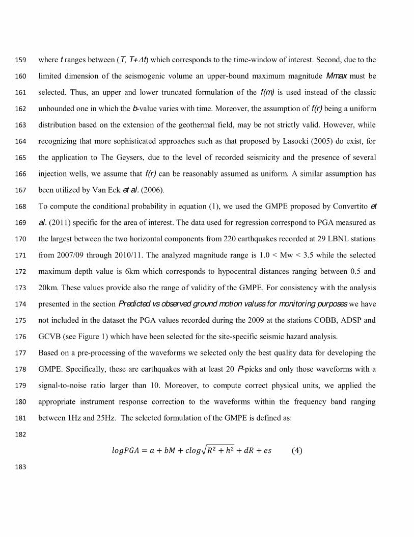
between 1Hz and 25Hz. The selected formulation of the GMPE is defined as:$!+!$

$!+'$

!+($

where PGA corresponds to peak-ground acceleration in m/s2. The distance metric R is the hypocentral !"#$

distance in km and M is the moment magnitude. Additionally, the h parameter is introduced to avoid !"%$

unrealistic high values at short distances (e.g., Joyner and Boore 1981; Emolo et al., 2011) and s !"&$

accounts for site effect. The coefficients and their uncertainties are listed in Table 1. We obtained the !"'$

best h value by minimizing the total standard error and maximizing the R2 statistic which measures how !""$

well the regression curve approximates the real data points (Draper and Smith, 1996). The obtained !"($

fictitious depth h = 3.5km yields the minimum standard error = 0.324 and a maximum R2 of 0.852. !()$

The need of developing a specific GMPE arises from the fact that the probability that published !(!$

GMPEs fail to predict peak-ground motion values from shallow-focus, small magnitude earthquakes is !(*$

high, as noted by Bommer et al. (2006) and, moreover, to date no other GMPEs published for The !(+$

Geysers geothermal field exist. Further, the use of a specific GMPE allows to account for possible !(#$

differences in static stress-drop conditions and anelastic attenuation between earthquakes induced !(%$

within geothermal fields and natural earthquakes occurring elsewhere. $!(&$

!('$

Seismic hazard analysis$!("$

Seismic source identification$!(($

Based on the earthquakes locations, magnitude distribution and the location of the injection wells, we *))$

divided the considered region at The Geysers into two source zones named ZONE1 (Z1) and ZONE2 *)!$

(Z2), which are outlined by the dashed lines shown in Figure 1. Our separation is supported by *)*$

arguments by Beall and Wright (2010), Beall et al. (2010) and Stark (2003) for The Geysers field. A *)+$

difference in the seismicity distribution has been also noted by Eberhart-Phillips and Oppenheimer *)#$

(1984). All the authors noted that the southeastern part of the Geysers reservoir is less active *)%$

seismically than the northwestern part where seismicity extends to greater depth. The difference was *)&$

basically ascribed to a depth variation in the high temperature (at 260-360°C) vapor dominated *)'$

*)"$

whole area into two different seismic areas. The northwestern area contains all the earthquakes with *)($

magnitude larger than 4.0 whereas the southeastern one is characterized by lower magnitude !"#$

earthquakes.$!""$

Moreover, the separation is justified from a statistical point of view by analyzing the b-values of the !"!$

Gutenberg-Richter relationship for the two areas using the Utsu (1992) test. The Utsu test allows to !"%$

verify that data used for estimating the b-values come from different populations, and hence are !"&$

associated with two different seismic sources. Using data for the entire duration of the analyzed catalog !"'$

starting from 2007 through 2010, we obtained a probability of the order of 1.0X10-6. $!"($

Maximum magnitude estimation$!")$

In studies dealing with induced seismicity, one of the most debated issue concerns the selection of the !"*$

maximum magnitude value, Mmax, that could be induced by field operations. As an example, Shapiro !"+$

et al. (2007) proposed a technique for estimating Mmax from an analysis of injection duration, the !!#$

strength of the injection source and rock properties such as hydraulic diffusivity. Recently, Shapiro et !!"$

al. (2010) also proposed the seismogenic index to quantify the seismotectonic state at an injection !!!$

location. The seismogenic index depends only on the tectonic features and is independent of injection !!%$

time or other injection characteristics, whose value correlates with the probability of significant !!&$

magnitude event. However, particularly for the period of interest analyzed in the present paper, detailed !!'$

data about injection rate and extraction rate are not freely available. As a consequence, we follow Van !!($

Eck et al. (2006) and estimate Mmax for each source zone by using the technique of Makropoulos and !!)$

Burton (1983), although it is based on a stationary assumption. The technique assumes that the total !!*$

energy, which may be accumulated and released in a seismogenic volume, is fairly constant in the !!+$

considered time window. This hypothesis can be considered valid if the whole duration of the analyzed !%#$

dataset is taken into account. Then, when the cumulative energy is plotted as function of time (Figure !%"$

2), the distance between the two parallel lines enveloping the released energy, correlates with the upper !%!$

limit of the energy that would be observed in the region, if the accumulated energy during the time was !%%$

released by a single earthquake. From the analyzed dataset we obtain Mmax values of 4.5 for Z1 and of !%&$

3.8 for Z2, respectively, as shown in Figure 2. These estimated values are coherent with the !%'$

observations reported in Table 2 which confirm that the magnitude M 4.5 has never been exceeded in !"#$

the analyzed period. $!"%$

Time-dependent seismicity parameters estimation$!"&$

Once the seismic sources are identified and the expected Mmax values are estimated, seismicity rate !"'$

and the b-value need to be calculated as function of time for the time-dependent PSHA. To this aim, we !()$

first estimated the minimum magnitude of completeness Mc of the available catalog by using a !(*$

technique similar to the Goodness-Of-Fit technique proposed by Wiemer and Wyss (2000). Basically, !(!$

the technique employs a comparison between the observed and the theoretical f(m) pdf with the aim of !("$

minimizing the root-mean square for a set of trial values for Mc, while the uncertainty is obtained by !(($

using a Monte Carlo approach. The results are shown in Figure 3b for Z1 and Figure 4b for Z2. Second, !(+$

we estimated the b-values by using the Aki (1965) technique, while their uncertainties are obtained !(#$

according to the formula of Shi and Bolt (1982). The obtained b-values are shown as gray dots in !(%$

Figure 3c for Z1 and in Figure 4c for Z2. The observed different temporal behavior of the two analyzed !(&$

parameters in Z1 and Z2 further supports the hypothesis of two different zones from the seismogenic !('$

point of view. The gray lines in the Figure 3d and 4d indicate the weekly seismicity rates, which !+)$

provide a detailed picture of the activity rate. However, for the purposes of performing a stable PSHA, !+*$

a monthly observation time is considered. A one-month time window permits to have a statistically !+!$

significant data sample for computing both the b-value and seismicity rate. The same time window has !+"$

been selected by Eberhart-Phillips and Oppenheimer (1984) and Majer and Peterson (2007) as it allows !+($

to catch the main features of the temporal seismicity evolution such as the difference between winter !++$

and summer months. Thus, assuming a non-homogenous Poisson model for earthquake occurrence, we !+#$

integrated the seismicity rate (t) in each time interval of one-month length and the resulting values !+%$

are plotted as black lines in Figure 3d for Z1 and Figure 4d for Z2. As a general consideration, it is !+&$

evident that the monthly seismicity rate level in Z1 is on average three times that in Z2. Particularly for !+'$

Z1 some interesting insights can be gained from the analysis of the plots. At a large time-scale, three !#)$

main peaks in the seismicity rate can be observed corresponding to March 2008, January 2009 and !#*$

November 2009, while the rate is quite constant between January 2010 and July 2010. In each year, a !#!$

seasonal variation of the seismicity rate can be noted, which is related to changes in the amount of !"#$

water injection throughout the year as shown in Figure 3a and Figure 4a. A similar observation has !"%$

been made by Majer and Peterson (2007) at The Geysers for the period from 2000 to mid 2006. !"&$

However, these observations must be accompanied with the analysis of Mc, which shows several !""$

fluctuations, particularly for Z2. This means that the catalogue has a variable minimum magnitude !"'$

completeness, which reflects several effects such as seismic network malfunctioning or improvements. !"($

Looking at the Mc value variation as function of time, in our present application, we choose to use only !")$

events with magnitude larger than 1.2 for subsequent analyses.$!'*$

As a further consideration, representing a key aspect for PSHA, the variations of the seismicity !'+$

rate and Mc also lead to a variation of the b-values. Figures 3c and 4c compare the temporal variation !'!$

of the b-values and their uncertainties with the seismicity rate for the two zones Z1 and Z2, !'#$

respectively. While the estimated b-values for Z2 show a large scatter, distinct trends can be seen for !'%$

Z1, corresponding to the periods September 2007 to January 2008, July 2008 to April 2009, May 2009 !'&$

to November 2009, and January 2009 to June 2010. Because the Mc values are stable within these !'"$

periods, these observed trends in the b-values can be considered as real features of the induced !''$

seismicity. Thus, it is expected that the probabilities of occurrence of larger magnitude earthquakes !'($

relative to lower magnitude events change in time and are different within the two zones. These !')$

temporal and spatial variations can affect the results of any PSHA and have to be included in such !(*$

analyses. $!(+$

$!(!$

Time-dependent hazard analysis $!(#$

Time-dependent PSHA proposed in the present paper utilizes a modified version of the technique !(%$

proposed by Convertito and Zollo (2011), which was originally developed for analyzing syn-crisis !(&$

seismicity before an impending volcanic eruption. In the present application, we calculate the !("$

seismicity rate and the b-values at several time intervals Tobs of one-month, and select four !('$

probabilities of exceedance: 30%, 50%, 70% and 90%. Taking an exposure time of 2 months, these !(($

probabilities correspond to return periods of about 6 months, 3 months, 2 months and 1 month, !()$

respectively. We chose the value of 2 months for the exposure time to account for at least two !"#$

variations in the time-window period used to collect data. $!"%$

We applied the GMPE reported in equation (4) to predict PGA, assuming that s = 0, which !"!$

corresponds to a rock-site condition. Concerning the GR relationship and the related magnitude PDF, !"&$

an upper bound on the magnitude values must be imposed. Here we chose a time varying truncated !"'$

version of f(m,b(t)) which is formulated as:$!"($

$!")$

In equation (5), =b(t)ln10, Mmax corresponds to the maximum magnitude value in each zone, i.e. !"*$

4.5 for Z1 and 3.8 for Z2, and the minimum magnitude of interest Mmin is set to 1.2 for both zones !"+$

which corresponds to the selected minimum magnitude of completeness. $!""$

To test the effect of the time variations of the input seismic parameters on the PSHA results, we &##$

computed hazard maps for different observation periods. The observation periods are 2008/08/10, &#%$

2009/02/06, 2009/09/04, 2010/03/03, 2010/06/01 and 2010/09/29, which are indicated by the squares &#!$

in the panels b, c and d of Figure 3 and Figure 4 for Z1 and Z2, respectively. Specifically, because we &#&$

have used a monthly representation for both the b-value and the seismicity rate , the indicated dates &#'$

represent the central value of the corresponding 1-month time period. We selected these specific &#($

periods to be able to monitor the different features of seismicity rate and b-values and to evaluate their &#)$

influence on PSHA. The corresponding hazard maps, showing the PGA values having 30%, 50%, 70% &#*$

and 90% of exceedance probabilities are shown in Figure 5. These maps illustrate that the hazard is not &#+$

constant in time. As an effect of the time variation of the seismic parameters, the largest PGA value &#"$

changes both in time and space. For example, for the first two observation periods (2008/08/10 and &%#$

2009/02/06) the zone with higher hazard is Z1, where PGA values as large as 4.5m/s2 are estimated as &%%$

values having 30% of probability of exceedance. On the other hand, largest PGA values are expected in &%!$

Z2 during the later observation periods (2010/03/03 and 2010/06/10). Because Z1 is characterized by a &%&$

larger Mmax value than Z2, the larger PGA values in Z2 during the later periods can be mainly !"#$

ascribed to the differences in the b-values. $!"%$

$!"&$

Predicted vs observed ground motion values for monitoring purposes $!"'$

As an additional analysis, we evaluated the use of PSHA as a monitoring tool to help to reduce seismic !"($

risk during the field operations. Benefitting from the availability of an independent dataset of PGA !")$

values for the analyzed period, we could follow a simple strategy to check the reliability of the PSHA !*+$

results. We compared the estimated PGA values with those PGA values actually recorded in the area !*"$

after the observation period considered for PSHA. In particular, we did a site-specific seismic hazard !**$

analysis at three sites named ADSP, COBB and GCVB (see Figure 1), considering the same !*!$

probabilities of exceedance as for the hazard maps computed in the Time-dependent Hazard Analysis !*#$

section. For each site and each of the selected Tobs we considered the successive three months and PGA !*%$

values. In particular, for the two sites ADSP and COBB data have been retrieved from the USGS (see !*&$

Data and Resources section) which, for the time period of interest, contains PGA values for 2009. For !*'$

the GCVB site, the NCEDC database (see Data and Resources section) has been accessed and PGA !*($

values were measured from the waveforms with the same procedure adopted for preparing the dataset !*)$

used for retrieving the GMPE. Thus the selected observation periods start at March, June and !!+$

September 2009, respectively. Before discussing the results it is important to note that in the case of !!"$

hazard associated with low-to-moderate magnitude earthquakes it might be more interesting to consider !!*$

the medium-to-highest probabilities instead of considering the lower ones as in the case of the standard !!!$

PSHA. This is because, for monitoring purposes it could be more relevant to know what actual ground-!!#$

motion level will be exceeded in the near future, rather than to assess the values associated with rare !!%$

events, which contribute more to the lowest probability of exceedance. $!!&$

The results of the site-specific PSHA in the monitoring context are shown in Figure 6. The estimated !!'$

PGA values resulting from the hazard analysis together with their associated probability of exceedance !!($

are indicated by the dashed horizontal lines. The observed PGA values are indicated by the gray !!)$

squares. Based on the recorded PGA values which are lower than 1.2 m/s2, all the sites experienced !#+$

light-to-moderate shaking, and the values predicted by the hazard analysis are consistent with these !"#$

observations. While the PGA values having 90% of probability of exceedance are systematically !"%$

exceeded, the PGA values having a 30% of probability of exceedance could be used if a cautious value !"!$

for a more conservative approach is needed. $!""$

$!"&$

Summary and Conclusions$!"'$

In this paper we suggested and applied a procedure for time-dependent probabilistic seismic hazard !"($

analysis in the context of the induced seismicity in geothermal reservoirs. The main aim consists in !")$

verifying that hazard levels produced by induced seismicity stay below critical values during all phases !"*$

of industrial operations. The analyzed dataset is made of waveforms and a parametric catalog of !&+$

earthquakes recorded at The Geysers geothermal field in Northern California between 2007/09/01 and !&#$

2010/11/15. $!&%$

Here we used a modified version of the approach proposed by Convertito and Zollo (2011) which is !&!$

based on the following main points that could be used as guidelines for a real monitoring application: $!&"$

- Identify the seismic source zones at The Geysers, considering both well locations and recorded !&&$

earthquakes (see Figure 1);$!&'$

- Estimate the expected maximum magnitude in each zone, that is 4.5 in Z1 (NW Geysers) and !&($

3.8 in Z2; $!&)$

- Compute the minimum magnitude of completeness Mc of the network and monitor its time-!&*$

variation (Mc set to 1.2 for the entire analyzed period); and$!'+$

- Compute the b-values and seismicity rates as functions of time (Figures 3 and 4). $!'#$

- Select proper critical ground motion thresholds related to potential damage or perceived !'%$

shaking.$!'!$

- Recalibrate field operations if predicted ground motion values exceed the thresholds. $!'"$

From all these parameters and their time-variation we obtained the time-dependent seismic hazard at !'&$

four probabilities of exceedance (30%, 50%, 70% and 90%), using PGA as the ground motion !''$

parameter of interest. The main result is that, based on the current value of the input parameters, !'($

seismic hazard at The Geysers is not constant in time and space. However, with reference to the values !"#$

used in ShakeMap® (Wald et al., 1999) the average hazard level remains below potential damaging !"%$

values. $!&'$

In addition, the availability of waveforms allowed us to investigate the possibility of using the !&($

time-dependent PSHA results for monitoring purposes. To this aim, we performed site-specific PSHA !&)$

at a set of observation times, which provided PGA values having given probabilities of exceedance, to !&!$

be used as predictions. We then compared these predicted PGA values with the PGA values observed !&*$

in the period after the respective observation time. The obtained results show that PGA values !&+$

corresponding to the lowest probability of exceedance (e.g., 30%) can be used as a conservative limit, !&"$

in accordance with the fact that lower probabilities are associated more to rare events. On the other !&&$

hand, the observations confirm that the predicted PGA values corresponding to higher probabilities of !&#$

exceedance are actually exceeded. $!&%$

A larger waveform database, together with the analysis of other ground motion parameters, !#'$

such as the PGV or the spectral ordinates at several structural periods, and possibly a longer study !#($

period seems to be necessary to justify and demonstrate the capabilities of time-dependent probabilistic !#)$

seismic hazard analysis as a monitoring tool during industrial operations. However, the results obtained !#!$

in the present study are encouraging, and we suggest testing our hazard analysis and monitoring !#*$

approach at other geothermal areas and, for example, also at gas field or carbon dioxide storage sites. $!#+$

$!#"$

Data and Resources$!#&$

Waveforms and parametric data have been retrieved from the National California Earthquake Data !##$

Center (NCEDC; network BG and station NC.GCVB; http://www.ncedc.org; last accessed on 20 !#%$

January 2012). The PGA values used for the analysis presented in the section Predicted vs observed !%'$

ground motion values for monitoring purposes have been retrieved from USGS !%($

(ftp://ehzftp.wr.usgs.gov/luetgert/calpine/sm_sum.txt, last accessed on 2012/04/24). Figures 3a and 4a !%)$

have been reproduced from an original figure by Calpine Corporation downloaded at !%!$

http://www.geysers.com/docs/20110818_Hartline_NW_Geysers_EGS_FINAL_Template.pdf (last !%*$

accessed on 20 January 2012). All figures have been generated with the Generic Mapping Tools !"#$

(Wessel and Smith, 1991). $!"%$

$!"&$

Acknowledgments !"'$

This work has been supported financially within the 7th Research Programme of the European Union !""$

through th gineering Integrating Mitigation of Induced Seismicity in ())$

; Contract number: 241321). The authors wish to thank the Associated ()*$

Editor Arthur McGarr and two anonymous reviewers whose suggestions improved the quality of the ()+$

manuscript. ()!$

()($

References$()#$

Aki, K. (1965). Maximum likelihood estimate of b in the formula logN=a-bM and its confidence limits. ()%$

Bull. Earthquake Res. Inst., 43, 237 239.$()&$

Allis, R. G. (1982), Mechanisms of induced seismicity at The Geysers geothermal reservoir, California. ()'$

Geophys. Res. Lett., 9, 629-632.$()"$

Bachmann, C. E., S. Wiemer, J. Woessner, and S. Hainzl (2011). Statistical analysis of the induced (*)$

Basel 2006 earthquake sequence: introducing a probability-based monitoring approach for (**$

Enhanced Geothermal Systems. Geophys. J. Int., 186(2), 793 807, doi: 10.1111/j.1365-(*+$

246X.2011.05068.x.$(*!$

Bazzurro, P. and C. A. Cornell (1999). Disaggregation of Seismic Hazard. Bull. Seismol. Soc. Am. 89, (*($

501-520. (*#$

Beall, J. J. and M. C. Wright (2010). Southern Extent of The Geysers High Temperature reservoir (*%$

based on seismic and geochemical evidence, Geothermal Resources Council Transactions, 34, 53-(*&$

56. (*'$

Beall, J.J., M.C. Wright, A. S. Pingol, and P. Atkinson (2010). Effect of high injection rate on (*"$

seismicity in The Geysers, Geothermal Resources Council Transactions, 34, 47-52. (+)$

Bommer, J. J., S. Oates, J. M. Cepeda, C. Lindholm, J. Bird, R. Torres, G. Marroquin, and J. Rivas !"#$

(2006). Control of hazard due to seismicity induced by a hot fractured rock geothermal project. !""$

Engineering Geology, 83, 287 306, doi: 10.1016/j.enggeo.2005.11.002. !"%$

Convertito, V., I. Iervolino, and A. Herrero (2009). Importance of mapping design earthquakes: !"!$

insights for the Southern Apennines, Italy. Bull. Seismol. Soc. Am., 99, 2979 2991, doi: !"&$

10.1785/0120080272. !"'$

Convertito, V., and A. Zollo (2011). Assessment of pre-crisis and syn-crisis seismic hazard at Campi !"($

Flegrei and Mt. Vesuvius volcanoes, Campania, southern Italy. Bull. Volcanol., 73, 767 783, !")$

doi: 10.1007/s00445-011-0455-2.$!"*$

Convertito, V., N. Sharma, N. Maercklin, A. Emolo, and A. Zollo (2011). Seismic hazard analysis as a !%+$

controlling technique of induced seismicity in geothermal systems. Fall Meeting, American !%#$

Geophysical Union, San Francisco, California, December 5 9, abstract S41C-2194. $!%"$

Cornell, C. A. (1968). Engineering seismic risk analysis. Bull. Seismol. Soc. Am., 58, 1583 1606.$!%%$

Draper, N. R., and H. Smith (1996). Applied regression analysis. New York. Third Edition, John Wiley !%!$

and Sons, Inc., 407 pp.$!%&$

Eberhart-Phillips, D., and D. H. Oppenheimer (1984), Induced seismicity in The Geysers Geothermal !%'$

Area, California. J. Geophys. Res., 89, 1191 1207.$!%($

Emolo A., V. Convertito, and L. Cantore (2011). Ground-Motion Predictive Equations for Low-!%)$

Magnitude Earthquakes in the Campania-Lucania Area, Southern Italy. J. Geophys. Eng. 8, 46!%*$

60, doi: 10.1088/1742-2132/8/1/007.$!!+$

Giardini, D. (2009). Geothermal quake risks must be faced. Nature 461, 848 849, doi: !!#$

10.1038/462848a. !!"$

Gutenberg, B., and C. R. Richter (1944). Frequency of earthquakes in California, Bull. Seism. Soc. Am. !!%$

34, 185 188. !!!$

Joyner, W. B., and D. M. Boore (1981). Peak horizontal acceleration and velocity from strong-motion !!&$

records including records from the 1979 Imperial Valley, California, earthquake. Bull. Seismol. !!'$

Soc. Am., 71, 2011 2038.$!!($

Lasocki, S. (2005). Probabilistic analysis of seismic hazard posed by mining induced events. In: Potvin !!"#

!!$#

-156. #!%&#

Makropoulos, K. C., and W. Burton (1983). Seismic risk of circum-Pacific earthquakes I. Strain energy !%'#

release. Pure Appl. Geophys., 121,247-266, doi: 10.1007/BF02590137. !%(#

Majer, E. L., and J. E. Peterson (2007). The impact of injection on seismicity at The Geysers, !%)#

California Geothermal Field. Int. J. Rock Mech. Mining Sci., 44, 1079 1090, doi: !%!#

10.1016/j.ijrmms.2007.07.023. !%%#

Majer, E. L., R. Baria, M. Stark, S. Oates, J. Bommer, B. Smith, and H. Asanuma (2007). Induced !%*#

Seismicity Associated with Enhanced Geothermal Systems. Geothermics, 36, 185-222. !%+#

Ogata, Y. (1988). Statistical models for earthquake occurrences and residual analysis for point-!%"#

processes. J. Am. Stat. Assoc., 83, 9 27. !%$#

Oppenheimer, D. C. (1986), Extensional tectonics at the Geysers Geothermal Area, California. J. !*&#

Geophys. Res., 91, 11463 11476. #!*'#

Reasenberg, P. A. and L. M. Jones (1989). Earthquake hazard after a mainshock in California. Science, !*(#

243, 1173-1176, doi: 10.1126/science.243.4895.1173. !*)#

Reiter, L. (1990). Earthquake hazard analysis. Columbia University Press, New York, 254 pp. !*!#

Shapiro, S. A., C. Dinske, and J. Kummerow (2007). Probability of a given-magnitude earthquake !*%#

induced by fluid injection. Geophys. Res. Lett., 34, L22314, doi: 10.1029/2007GL031615. !**#

Shapiro, S. A., C. Dinske, and C. Langenbruch (2010). Seismogenic index and magnitude probability !*+#

of earthquakes induced during reservoir fluid stimulation. The Leading Edge, 29, 304 309, doi: !*"#

10.1190/1.3353727. #!*$#

Shi, Y., and B. A. Bolt (1982). The standard error of the magnitude-frequency b value. Bull. Seismol. !+&#

Soc. Am., 72,1677 1678.#!+'#

Stark, M. (2003). Seismic Evidence for A Long-Lived Enhanced Geothermal System (EGS) in the !+(#

Northern Geysers Reservoir, Geothermal Resources Council Transactions, 27, 727-731.#!+)#

Utsu, T. (1992). On seismicity. In: Report of Cooperative Research of the Institute of Statistical !"!#

Mathematics 34, Mathematical Seismology VII, Annals of the Institute of Statistical !"$#

Mathematics, Tokio, 139 157. #!"%#

Van Eck, T., F. Goutbeek, H. Haak, and B. Dost (2006). Seismic hazard due small-magnitude, shallow-!""#

source, induced earthquakes in The Netherlands. Engineering Geology 87, 105 121, doi: !"&#

10.1016/j.enggeo.2006.06.005.#!"'#

Wald, D. J., V. Quitoriano, T. H. Heaton, H. Kanamori, C. W. Scrivner, and C. B. Worden (1999). !&(#

TriNet "ShakeMaps": Rapid Generation of Peak Ground motion and Intensity Maps for !&)#

Earthquakes in Southern California. Earthquake Spectra 15, 537 556, doi: 10.1193/1.1586057. !&*#

Wiemer, S., and M. Wyss (2000). Minimum magnitude of completeness in earthquake catalogs: !&+#

examples from Alaska, the Western United States, and Japan, Bull. Seismol. Soc. Am. 90, 859!&!#

869. !&$#

Wessel, P., and W. H. F. Smith (1991). Free software helps map and display data, EOS Trans. AGU, !&%#

72, 445 446. !&"#

#!&&#

Affiliations#!&'#

1. Istituto Nazionale di Geofisica e Vulcanologia, Osservatorio Vesuviano, Via Diocleziano 328, 80124 !'(#

Napoli, Italy.#!')#

2. AMRA S.c.a.r.l., Analysis and Monitoring of Environmental Risk, Via Nuova Agnano 11, 80125 !'*#

Napoli, Italy.#!'+#

3. !'!#

Universitario di Monte S. Angelo, Via Cintia, 80126 Napoli, Italy. #!'$#

!'%#

Tables#!'"#

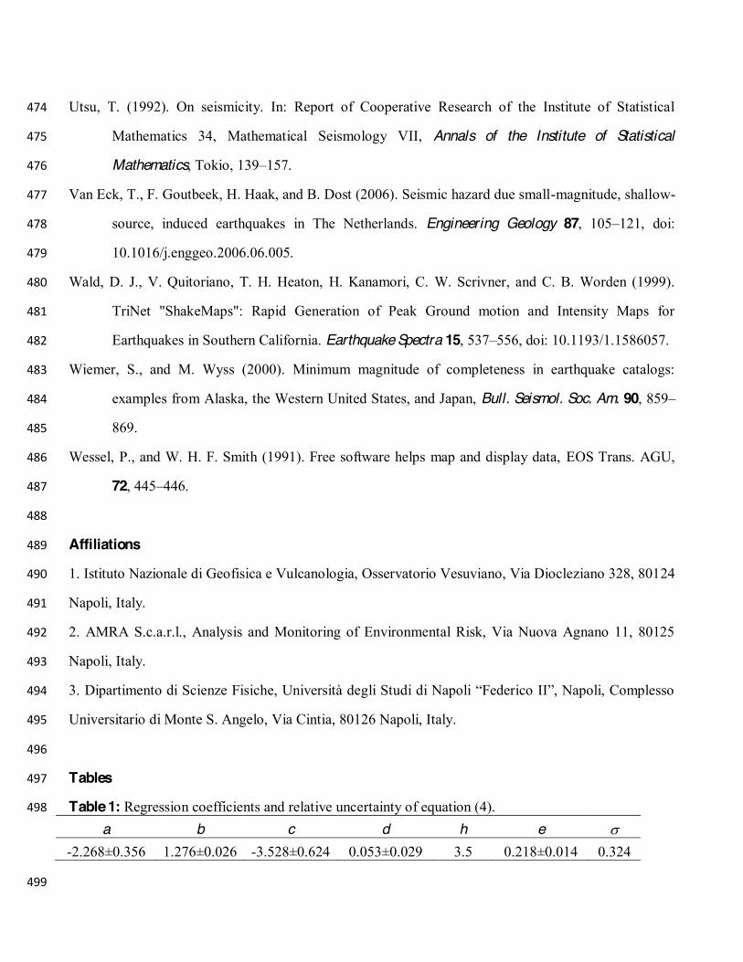
Table 1: Regression coefficients and relative uncertainty of equation (4). #!'&#

a# b# c# d# h# e# #

-2.268±0.356# 1.276±0.026# -3.528±0.624# 0.053±0.029# 3.5# 0.218±0.014# 0.324#

#!''#

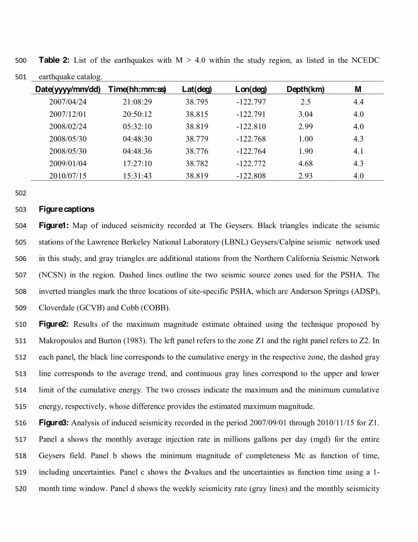
Table 2: List of the earthquakes with M > 4.0 within the study region, as listed in the NCEDC !""#

earthquake catalog. #!"$#

Date(yyyy/mm/dd)# Time(hh:mm:ss)# Lat(deg)# Lon(deg)# Depth(km)# M #

2007/04/24# 21:08:29# 38.795# -122.797# 2.5# 4.4#2007/12/01# 20:50:12# 38.815# -122.791# 3.04# 4.0#2008/02/24# 05:32:10# 38.819# -122.810# 2.99# 4.0#2008/05/30# 04:48:30# 38.779# -122.768# 1.00# 4.3#2008/05/30# 04:48:36# 38.776# -122.764# 1.90# 4.1#2009/01/04# 17:27:10# 38.782# -122.772# 4.68# 4.3#2010/07/15# 15:31:43# 38.819# -122.808# 2.93# 4.0#

!"%#

Figure captions#!"&#

Figure1: Map of induced seismicity recorded at The Geysers. Black triangles indicate the seismic !"'#

stations of the Lawrence Berkeley National Laboratory (LBNL) Geysers/Calpine seismic network used !"!#

in this study, and gray triangles are additional stations from the Northern California Seismic Network !"(#

(NCSN) in the region. Dashed lines outline the two seismic source zones used for the PSHA. The !")#

inverted triangles mark the three locations of site-specific PSHA, which are Anderson Springs (ADSP), !"*#

Cloverdale (GCVB) and Cobb (COBB). !"+#

Figure2:# Results of the maximum magnitude estimate obtained using the technique proposed by !$"#

Makropoulos and Burton (1983). The left panel refers to the zone Z1 and the right panel refers to Z2. In !$$#

each panel, the black line corresponds to the cumulative energy in the respective zone, the dashed gray !$%#

line corresponds to the average trend, and continuous gray lines correspond to the upper and lower !$&#

limit of the cumulative energy. The two crosses indicate the maximum and the minimum cumulative !$'#

energy, respectively, whose difference provides the estimated maximum magnitude. #!$!#

Figure3: Analysis of induced seismicity recorded in the period 2007/09/01 through 2010/11/15 for Z1. !$(#

Panel a shows the monthly average injection rate in millions gallons per day (mgd) for the entire !$)#

Geysers field. Panel b shows the minimum magnitude of completeness Mc as function of time, !$*#

including uncertainties. Panel c shows the b-values and the uncertainties as function time using a 1-!$+#

month time window. Panel d shows the weekly seismicity rate (gray lines) and the monthly seismicity !%"#

rate (black lines). The squares identify the dates of the selected observation periods at which seismic !"#$

hazard analysis has been performed.$!""$

Figure4:$Same as Figure 3, but for Z2. $!"%$

Figure5: Seismic hazard maps relative to the dates indicated by the squares in Figure 3 and Figure 4. !"&$

The reported PGA are expressed in m/s2 and represent the peak-ground motion values having the !"!$

probability of exceedance reported on the top of each map. Each date corresponds to the central time of !"'$

a 1-month window centered on that date. The dashed lines outline the two seismic zones shown in !"($

Figure1. $!")$

Figure6: Site specific seismic hazard analysis for the three sites indicated in Figure 1. The analysis has !"*$

been performed for three observation periods starting at 2009/03/03 (panel a), 2009/06/01 (panel b) and !%+$

2009/09/29 (panel c), respectively, and whose duration is three months. The dashed horizontal lines !%#$

correspond to the result of the PSHA at the indicated probability of exceedance. Gray squares represent !%"$

the PGA values observed at the specific station. $!%%$

$!%&$

$!%!$

$!%'$

$!%($

$!%)$

$!%*$

$!&+$

$!&#$

$!&"$

$!&%$

$!&&$

$!&!$$!&'$

$!&($

$!&)$

!"#$!

Figure 1!""%!

!""&!

!""'!

!""(!

!""#!

!"""!

!"")!

!""*!

!""+!

!""#!

!"$%!

!"$&!

!"$'!

!"$(!

Figure 2!"$)!

!"$"!

!"$$!

!"$*!

!"$+!

!"$#!

!"*%!

!"#$

Figure 3$!"%$

$!"&$

!"#$!

Figure 4!"#"!

"#%!

Figure 5 !""#

!"#$!

Figure 6!"#%!