from listing data to semantic maps: cross … · cross-linguistic commonalities in cognitive...

http://dx.doi.org/10.7592/FEJF2016.64.colour

FROM LISTING DATA TO SEMANTIC MAPS: CROSS-LINGUISTIC COMMONALITIES IN COGNITIVE REPRESENTATION OF COLOUR

Mari Uusküla, David Bimler

Abstract: When a free-listing task is used to elicit verbal concepts from a given semantic domain, it provides two indicators of the salience of each word for that linguistic community. These are the proportion of the subjects who include a word in their lists, and its average ranking priority position across the lists. The data also contain cues about the cognitive representation of the semantic domain, and in particular about the conceptual closeness among words. Closely associated words tend to prime each other and to appear in the lists in close succession. Clusters of mutually associated terms can be recognised, listed in one another’s company, although with different priority for different subjects. We applied this approach to the domain of colour terms, converting lists for fourteen European languages into matrices of inter-term similarity, for analysis with multidimen-sional scaling (MDS) and hierarchical clustering. Two-dimensional MDS solutions or ‘maps’ were typically required to reflect two competing criteria by which terms were sequenced. Speakers of each language tended to follow a salience gradient, but also made separate clusters of fully-chromatic concepts – colour terms in strictu sensu – and unsaturated or desaturated concepts defined primarily by lightness rather than by hue. This and other features recurred across the lan-guages despite their geographical and phylogenetic diversity, as cross-cultural universals in colour language, in addition to the well-known regularities governing basic colour terms and the stages of colour-lexicon development.

Keywords: basic colour terms, Cognitive Salience Index, colour language, cross-linguistic comparison, linguistic typology, listing task, multidimensional scaling

INTRODUCTION

In the Method of Listing, a semantic domain is specified, such as ‘colour terms’ or ‘animal names’, and participants are asked to list all the examples of the domain they can think of, in the order in which they come to mind. These lists contain information about the salience of the terms (Borgatti 1999; Weller & Romney 1988). Thus the Listing Method is a useful tool for determining which colour terms in a given language deserve to be singled out as Basic Colour Terms or BCTs (Corbett & Davies 1997; Jrassati et al. 2012): that is, ‘natural classes’,

http://www.folklore.ee/folklore/vol64/colour.pdf

58 www.folklore.ee/folklore


the default level of specificity for classifying and communicating about colours. Crucially, languages differ in the number of BCTs.

The concept was introduced by Berlin and Kay (1991 [1969]), although details of the definition and the criteria of ‘basicness’ have subsequently evolved (one might speak of a continuous scale of basicness underlying the dichotomy between ‘basic’ and ‘non-basic’ (Kerttula 2007)). The argument here is that a non-basic term features in the productive lexicons of fewer speakers than a BCT, and those who do list it, do so later in their sequences. Smith, Furbee, Maynard, Quick and Ross (1995) ranked English colour terms in order of decreasing salience, and separated them into three distinct classes: BCTs; non-basics, which they subdivided into ‘opaque’ and ‘transparent’; and ‘complex’ terms (plus a ‘residual’ category, which includes textures and patterns).

Using the index ‘i’ to identify the terms, we can write ni as the number of speakers who listed the i-term, and ni / N as the proportion, where N is the total number of sequences collected. We can also write mri as the mean rank of that term across those ni sequences. Both indicators of salience have been published in a number of studies of a variety of languages (e.g. Davies & Corbett 1994a, 1994b; Davies & Corbett & Margalef 1995; Hippisley 2001). Urmas Sutrop (2001) combined them in the Cognitive Salience Index, CSI(i) = ni / N / mri. The goal of this study is to extend this approach.

A useful model for thinking about the listing task is the image of a ‘semantic network’ or a ‘semantic map’. Terms are imagined as nodes in the network, connected by links, with activation spreading between the nodes which is faster along stronger and more direct links (e.g. Collins & Loftus 1975; Goñi et al. 2011). The participant initially accesses the network through some especially prototypical or culturally-salient node (e.g. ‘red’), and then explores it more-or-less systematically, as one term prompts the recollection of its neighbours; tending to progress down the gradient of salience, at each step following a link or association to whichever node has received most activation, until the bound-ary of the semantic domain is reached.

Thus a corpus of listing sequences contains additional structure about the pattern of associations and inter-relationships among the terms (non-basic colour terms as well as BCTs), to be extracted by more sophisticated analysis. If participants tend to list a pair of terms in close proximity – one term often immediately preceding or following the other – this is suggestive of a close con-ceptual link between them. In a precedent from the domain of animal names, Henley (1969) obtained a matrix of estimated inter-name link strength from listing data by averaging the ‘adjacency’ between each pair of terms (i.e. the absolute difference in the terms’ sequence positions) across participants. Al-though each individual’s personal network is unique, here we treat them as

Folklore 64 59

From Listing Data to Semantic Maps

approximations of a single cultural consensus. That is, the individual lists are conceived as coming from that consensus network (perturbed by random fluctuations), which we set out to reconstruct.

Despite the network metaphor, it is convenient to summarise the pattern of associations in terms of a spatial model. Here items are represented as points, arranged in a low-dimensional space so that proximity between each pair of terms reflects the average adjacency of corresponding terms. Another useful model is a hierarchical-clustering ‘tree’: a structure of successively forking branches, with terms at the ‘leaves’, so that all the leaves arising from one branch define a cluster (nested within larger clusters). Again, the distance between leaves – measured down one branch to a fork and up the other branch – reflects (dis‑)similarity. Shepard (1974) applied multidimensional scaling or MDS to a matrix of animal-name adjacencies, and extracted a parsimonious, two-dimensional spatial map with interpretable axes. In a further replication of Henley’s work, Storm (1980) elicited lists from subjects across six age bands, although the matrices of pairwise differences resisted reduction to a low-dimensional MDS solution.

The same analysis is also applicable to recall data in which participants at-tempt to recall terms from a list that was read to them (for instance, Friendly 1979, whose examples again include animal names). The focus here is on the clustering of items in the MDS or tree solution, i.e. how items were organised by memory into thematic ‘chunks’. Having recalled one item from a ‘chunk’, the participant finds it easier to access others and exhaust the semantic cluster before continuing to another (e.g. Goñi et al. 2011). We expect to encounter this modular structure here: self‑contained sub‑lists of colour terms, which flock together, though appearing at different positions in different participants’ lists.

Although we are interpreting list adjacency in terms of ‘similarity’, this is a conceptual, not a perceptual connection. Associational connection can stem from a contrast, or an antagonism, as much as from the number of features the two items share. Cultural associations and collocations contribute to their mutual priming. We sourced listing data from 14 languages, from three dif-ferent language phyla – Indo-European, Uralic and Altaic – though all were European, and in cultural contact with their neighbours. We are interested in the extent of commonality across the MDS solutions. In other words, do the different language communities impose similar patterns of thematic and dimensional organization upon their colour lexicon?

One development in colour linguistics has been the recognition of common threads across cultures in terms of BCTs and the corresponding perceptual categories. Languages vary in the size of their colour lexicon, and the terms themselves may not be exact counterparts. A parsimonious inventory of focal



hues accounts for a large proportion of linguistic variability (i.e. the prototype hues, chosen as the best example of each category), with languages diverging primarily in how many of these foci they recognise as the nuclei of categories (Regier & Kay & Cook 2005). In Guatemala, Harkness (1973) observed that speakers of Mam (a Mayan language) partitioned colour space into fewer colour categories than their Spanish-speaking neighbours, but the foci of those cat-egories each had a counterpart from the Spanish foci. The Namibian language Himba and the Papua‑New‑Guinea language Berinmo both recognise five BCTs, but dumbu in Himba is not quite equivalent to wor in Berinmo (Roberson et al. 2004): different boundaries in colour space distinguish these categories from neighbouring categories. Nevertheless, their foci are very similar.

Thus it is reasonable to look for recurring patterns in colour-lexicon seman-tic networks, albeit purely cognitive patterns, in contrast to the perceptual / conceptual universals noted by Berlin and Kay.

METHOD

Procedure

Data were collected in the course of a standard interview for establishing the BCTs in a language, in which participants also performed a colour-naming task subsequent to the listing task (Corbett & Davies 1997). The participants were blind to the topic as they were recruited to ‘answer questions regarding their native language’. They were requested to ‘Please name as many colours as you know’ in their L1. Time allocated for listing and the length of the list were not limited. All elicitation data was gathered orally and written down (and/or recorded) by the experimenter, except for the Swedish and English groups who wrote their responses.

Languages and participants

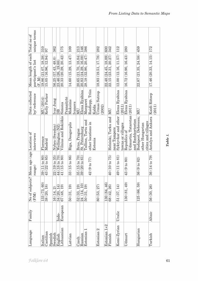
The sample contains 14 languages belonging to the Indo-European, Uralic and Altaic families. Between them, these languages are spoken in a vast territory of Eurasia. The distribution of languages according to family is presented in Table 1, along with numbers of participants and other information.

Present Udmurt participants were divided between speakers of Northern and Southern Udmurt dialects, in which ‘pink’ is translated as lemlet and ljölj respectively (many of the present participants knew both terms and listed them consecutively). Southern dialects also possess the BCTs kuren’ ‘brown’ and

Folklore 64 61


Lan

guag

eF

amil

yN

o of

su

bjec

ts?

(F/M

)M

ean

age

(ag

e ra

nge

)L

ocat

ion

of

inte

rvie

ws

Dat

a co

llec

ted

by/ r

efer

ence

Mea

n le

ngt

h o

f ea

ch

part

icip

ant’s

list

(F

, M)

Tot

al n

o of

u

niq

ue

term

s

Ital

ian

133

(73,

60)

39 (

11 t

o 80

)F

lore

nce

MU

(20

14)

19.8

6 (2

1.07

, 18.

38)

310

Cas

tili

an

Spa

nis

h38

(20

, 18)

43 (

22 t

o 85

)M

adri

dK

elly

Par

ker

15.0

5 (1

6.96

, 12.

94)

97

Sw

edis

h16

(14

, 2)

22 (

19 t

o 35

)N

ybro

(S

wed

en)

Ivar

Ju

ng

56.2

5 (5

7.43

, 48.

0)36

2E

ngl

ish

Indo

-34

(20

, 14)

44 (

18 t

o 70

)W

elli

ngt

on (

NZ

)D

B23

.46

(26,

19.

88)

Lit

hu

ania

nE

uro

pean

67 (

48, 1

9)41

(15

to

80)

Vil

niu

s an

d R

okiš

kis

Sim

ona

Pra

nai

tytė

20.3

3 (2

0.29

, 20.

42)

175

Lat

vian

50 (

31, 1

9)33

(15

to

86)

Rīg

a, D

auga

vpil

sM

aksi

ms

Ivan

ovs

14.6

0 (1

5.29

, 13.

47)

109

Cze

ch52

(33

, 19)

35 (

15 t

o 70

)B

rno,

Pra

gue

MU

20.6

5 (2

1.70

, 18.

84)

213

Ru

ssia

n24

(14

, 10)

39 (

20 t

o 61

)S

t. P

eter

sbu

rgE

len

a R

yabi

na

20.8

3 (2

4.29

, 16.

00)

146

Est

onia

n 1

50 (

31, 1

9)42

(9

to 7

7)T

alli

nn

, Tar

tu a

nd

oth

er lo

cati

ons

in

Est

onia

Mar

gare

t R

aidl

epp,

Tri

in

Kal

da

28.1

8 (3

2.90

, 20.

47)

386

Est

onia

n 2

80 (

53, 2

7)U

rmas

Su

trop

(2

002)

18.9

3 (1

9.51

, 17.

78)

282

Est

onia

n 1

+213

0 (8

4, 4

6)22

.48

(24.

45, 1

8.89

)60

0F

inn

ish

68 (

42, 2

6)40

(10

to

75)

Hel

sin

ki, T

urk

u a

nd

nea

r T

ampe

reM

U22

.15

(23.

31, 2

0.27

)34

2

Kom

i-Z

yria

nU

rali

c51

(37

, 14)

49 (

11 t

o 81

)S

ykty

vkar

an

d ot

her

to

wn

s or

vil

lage

sE

len

a R

yabi

na

(201

1)12

.00

(12.

16, 1

1.57

)11

2

Udm

urt

130

(81,

49)

43 (

9 to

80)

Rep

ubl

ics

of

Udm

urt

ia, T

atar

stan

an

d B

ash

kort

osta

n

Ele

na

Rya

bin

a (2

011)

16.7

2 (1

6.90

, 16.

43)

280

Hu

nga

rian

125

(66,

59)

36 (

9 to

82)

Bu

dape

st, D

ebre

cen

; ot

her

Hu

nga

rian

ci

ties

an

d vi

llag

es

MU

22.8

7 (2

1.35

, 24.

58)

459

Tu

rkis

hA

ltai

c56

(30

, 26)

36 (

14 t

o 79

)A

nta

lya

and

An

kara

Kai

di R

ätse

p (2

011)

17.4

6 (2

0.33

, 14.

15)

172

Ta

ble

1.



nap-čuž ‘orange’ but in Northern dialects no single term is assigned to orange and brown stimuli consistently enough to qualify for basicness. The language possesses the term busir ‘purple’, but this is not known to all language speak-ers (Ryabina 2011).

All subjects were recruited volunteers, with a representative sample of speak-ers – as a rule of thumb, Weller and Romney (1988) recommend a minimum of 20 to 30 informants. The sampling was random. Participants had different dialectal, educational and social backgrounds. The interviews were carried out by a native speaker (for Lithuanian, English, Estonian, and Udmurt) or a proficient L2 speaker (for all other languages). All subjects were screened for normal colour vision using pseudoisochromatic plates (Ishihara 2008) or the City University test (Fletcher 1980).

Data for 80 of the 130 Estonian subjects were collected by Urmas Sutrop in his 2002 study.

For three of the languages, additional data were available from participants in a separate study that focussed on terms used in the blue region of colour space (Bimler & Uusküla, in preparation). That study featured colour sorting as well as the naming task, but not all participants performed the listing task. Specifically: of the 133 Italian subjects, 102 participated in the main study, while 31 lists came from 54 participants in the second study. Of the 67 Lithuanian subjects, 51 participated in the main study, while 16 lists came from 50 par-ticipants in the separate study. Of the 130 Udmurt subjects, 125 participated in the main study, while 5 lists came from 25 participants in the second study.

Analysis

As noted above, the Cognitive Salience Index for items generated in listing data (Sutrop 2001) combines two sources of information: the proportion of par-ticipants to whom a term occurs, and the stage at which it occurred to those participants, i.e. its priority in their lists.

CSI(i) = ni / N / mri

Smith (1993) defined a salience index S, which is similarly a confluence of frequency and priority (also Smith et al. 1995). However, the tables of ni and mri that have been published for a number of languages (e.g. Davies & Corbett 1994a, 1994b; Davies & Corbett & Margalef 1995; Hippisley 2001) are not suf-ficient for calculating S(i).

Folklore 64 63


Following Henley (1969) and Friendly (1977), we defined a measure of ad-jacency ADJ(i,j) between the i-th and j-th terms. A matrix of separations SEPp is obtained for the p-th subject, with entries

SEPpij = ln | spi – spj |.

This definition incorporates information from listing data beyond immediate-ly-sequential items. Even if a participant does not list term B directly after term A, we assume that the activation of A persists, increasing the probability that B will be listed subsequently; with the corollary that more remote separa-tion, such as the appearance of B two steps rather than three steps after A, is still an indication of the association between them.

The number of participants for whom SEPpij is defined (because they included both terms i and j in their sequences) is cij, the co-occurrence of that pair of terms. Then ADJ(i,j) uses the mean of the separations, averaged across only those participants:

ADJ(i,j) = exp [(Σp SEPpij) / cij].

The effect of the logarithmic transform in SEPpij is that ADJ is the geometric mean of absolute differences rather than the arithmetic mean. This is so that an increment to a small separation (such as the difference between two consecu-tive terms, where SEPpij = 0, and terms separated by an intermediary, where SEPpij = ln 2) has more effect on the value of ADJ(i,j) than the same increment for more widely separated terms.

Not all the terms nominated in each language were included in the analy-sis; only the more salient ones, for which the associations ADJ(i,j) with other terms could be estimated with some confidence. The reliability of each esti-mate depends on the co-occurrence cij, and is limited by statistical fluctuations: ADJ(i,j) is less reliable when the i-th and j-th terms are both low-salience so they co-occur only in the lists of a few unrepresentative participants. Naturally this threshold of confidence allowed more terms to be considered in language samples for which more participants were recruited, or if these recruits were relatively productive.

Adjacency matrices were analysed with MDS, using the PROXSCAL software within SPSS to represent terms as points in a low-dimensional space. Ordinal transforms were used (the non-metric form of MDS), with the tie-breaking option. We retained two-dimensional solutions to allow them to be compared across languages, including those for which fewer items could be analysed reli-ably and a third axis could not be justified.

PROXSCAL allows the entries in a proximity matrix to be weighted by reli-ability (less‑reliable entries having less influence in determining the locations of



the two corresponding items). We entered the square root of co-occurrences, √ cij, for this purpose. To ensure that the algorithm converged towards the overall best fit rather than being trapped in a ‘local minimum’, starting configurations were randomised, iterating over 500 random starts for each matrix.

Hierarchical clustering was applied using Ward’s algorithm, implemented in SPSS 20. Note that non-metric models are not applicable for HCA, i.e. the analysis necessarily assumes that the (postulated) underlying similarities among items follow a linear relationship to the estimates obtained from the data. In addition, there is no option for including information about the reli-ability of individual estimates.

RESULTS

Some basic statistics for the lists are included in Table 1: mean length of each participant’s list (with separate values for males and females), plus the to-tal number of unique terms nominated. Productivity ranged from a mean of 12 terms per list for Komi-Zyrian, up to 56.25 for Swedish. Swedish was a spe-cial case; the instructions were evidently understood differently than in other samples, as if participants felt called upon to list all the terms they could think of, perhaps to make up for the small sample size. Swedish participants were all art or design students, who recorded their lists in writing, in constrast to other groups who gave oral responses. The distributions of terms per list listp were strongly skewed, so the following analyses were performed on log(listp) to produce more normal distributions.

ANOVA confirmed the reality of this variation, with a significant effect from the independent variable ‘language group’ (F = 14.25, 13 d.f., p < 0.001). The contribution to variance from the variable ‘gender’ was also significant, with women tending to list more terms than men (F = 21.33, 1 d.f., p < 0.001). However, this was not consistent across languages, i.e. a gender-by-language interaction term also reached significance (F = 2.24, 13 d.f., p = 0.07). In analyses of each sample in isolation, the male/female difference was significant for five languages: English: (t = 2.43, p = 0.02), Estonian (t = 2.85, p = 0.005), Italian (t = 2.13, p = 0.035, Spanish (t = 5.70, p = 0.022), and Turkish (t = 3.21, p = 0.002).

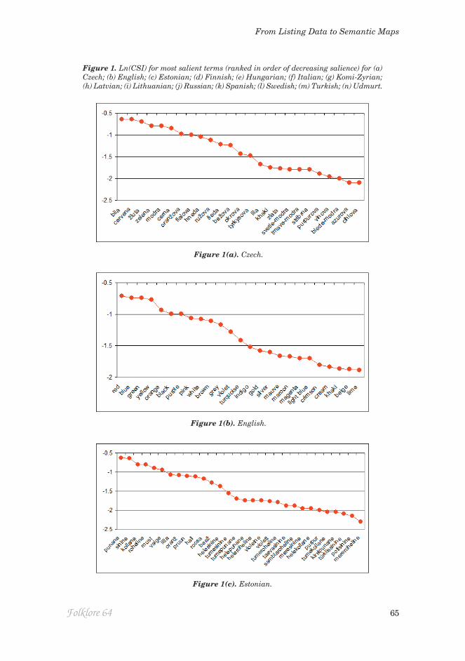
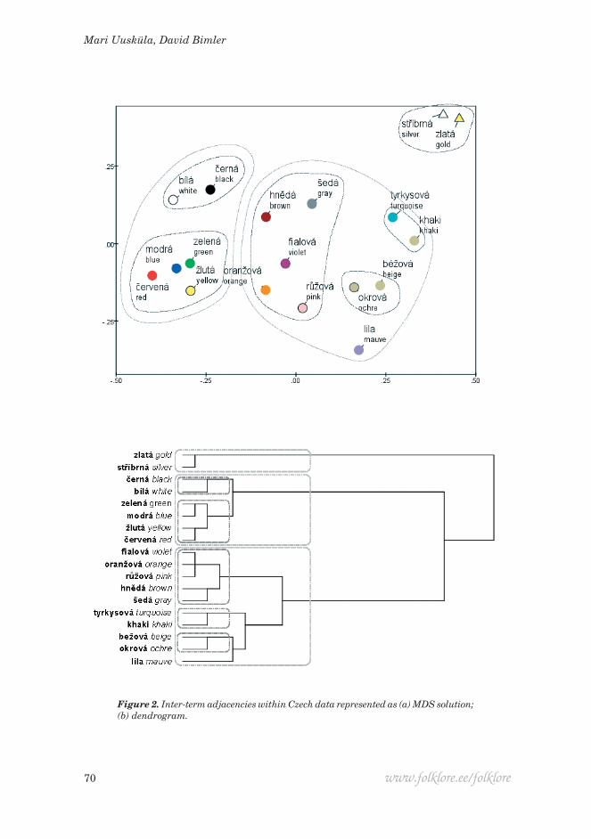
Figure 1(a) shows CSI values for the 25 most salient terms in Czech, while Figure 2(a) is the MDS solution for the most frequent terms, using Czech as a simple but representative case. When terms are ranked in order of decreasing salience, the values typically follow a roughly exponential decline. Figure 1(a) exploits this generalisation by plotting CSI on a logarithmic scale, to render the decline roughly linear.

Folklore 64 65


Figure 1(a). Czech.

Figure 1(b). English.

Figure 1(c). Estonian.

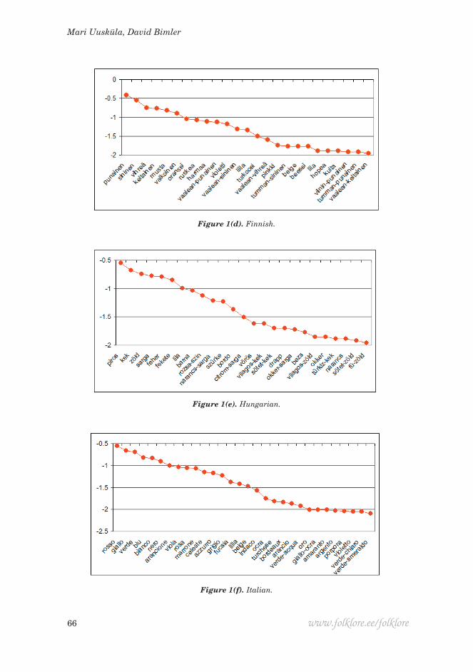
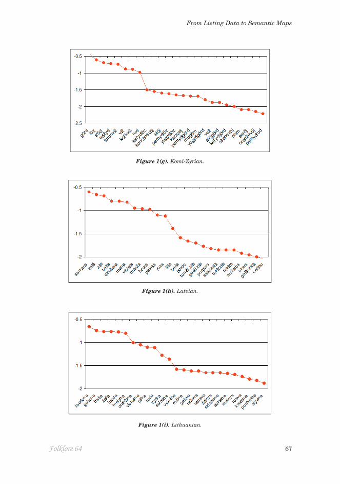
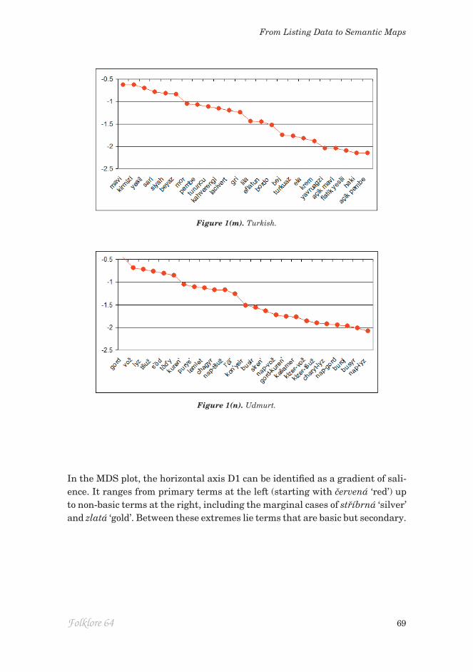
Figure 1. Ln(CSI) for most salient terms (ranked in order of decreasing salience) for (a) Czech; (b) English; (c) Estonian; (d) Finnish; (e) Hungarian; (f) Italian; (g) Komi-Zyrian; (h) Latvian; (i) Lithuanian; (j) Russian; (k) Spanish; (l) Swedish; (m) Turkish; (n) Udmurt.



Figure 1(d). Finnish.

Figure 1(e). Hungarian.

Figure 1(f). Italian.

Folklore 64 67


Figure 1(g). Komi-Zyrian.

Figure 1(h). Latvian.

Figure 1(i). Lithuanian.



Figure 1(j). Russian.

Figure 1(k). Spanish.

Figure 1(l). Swedish.

Folklore 64 69


Figure 1(m). Turkish.

Figure 1(n). Udmurt.

In the MDS plot, the horizontal axis D1 can be identified as a gradient of sali-ence. It ranges from primary terms at the left (starting with červená ‘red’) up to non-basic terms at the right, including the marginal cases of stříbrná ‘silver’ and zlatá ‘gold’. Between these extremes lie terms that are basic but secondary.



Figure 2. Inter-term adjacencies within Czech data represented as (a) MDS solution; (b) dendrogram.

Folklore 64 71


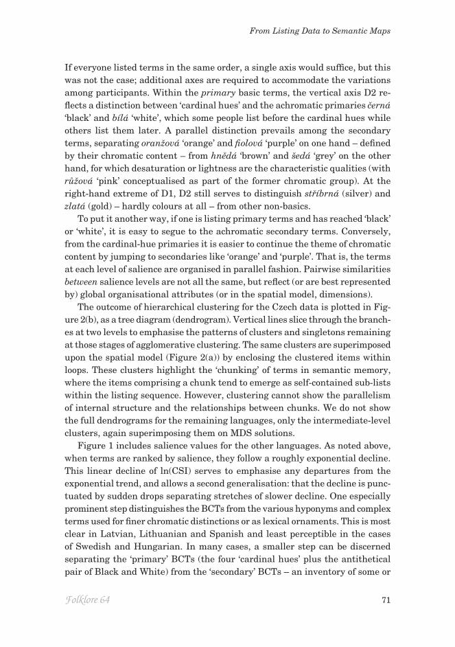
If everyone listed terms in the same order, a single axis would suffice, but this was not the case; additional axes are required to accommodate the variations among participants. Within the primary basic terms, the vertical axis D2 re-flects a distinction between ‘cardinal hues’ and the achromatic primaries černá ‘black’ and bílá ‘white’, which some people list before the cardinal hues while others list them later. A parallel distinction prevails among the secondary terms, separating oranžová ‘orange’ and fiolová ‘purple’ on one hand – defined by their chromatic content – from hnědá ‘brown’ and šedá ‘grey’ on the other hand, for which desaturation or lightness are the characteristic qualities (with růžová ‘pink’ conceptualised as part of the former chromatic group). At the right-hand extreme of D1, D2 still serves to distinguish stříbrná (silver) and zlatá (gold) – hardly colours at all – from other non-basics.

To put it another way, if one is listing primary terms and has reached ‘black’ or ‘white’, it is easy to segue to the achromatic secondary terms. Conversely, from the cardinal-hue primaries it is easier to continue the theme of chromatic content by jumping to secondaries like ‘orange’ and ‘purple’. That is, the terms at each level of salience are organised in parallel fashion. Pairwise similarities between salience levels are not all the same, but reflect (or are best represented by) global organisational attributes (or in the spatial model, dimensions).

The outcome of hierarchical clustering for the Czech data is plotted in Fig-ure 2(b), as a tree diagram (dendrogram). Vertical lines slice through the branch-es at two levels to emphasise the patterns of clusters and singletons remaining at those stages of agglomerative clustering. The same clusters are superimposed upon the spatial model (Figure 2(a)) by enclosing the clustered items within loops. These clusters highlight the ‘chunking’ of terms in semantic memory, where the items comprising a chunk tend to emerge as self-contained sub-lists within the listing sequence. However, clustering cannot show the parallelism of internal structure and the relationships between chunks. We do not show the full dendrograms for the remaining languages, only the intermediate-level clusters, again superimposing them on MDS solutions.

Figure 1 includes salience values for the other languages. As noted above, when terms are ranked by salience, they follow a roughly exponential decline. This linear decline of ln(CSI) serves to emphasise any departures from the exponential trend, and allows a second generalisation: that the decline is punc-tuated by sudden drops separating stretches of slower decline. One especially prominent step distinguishes the BCTs from the various hyponyms and complex terms used for finer chromatic distinctions or as lexical ornaments. This is most clear in Latvian, Lithuanian and Spanish and least perceptible in the cases of Swedish and Hungarian. In many cases, a smaller step can be discerned separating the ‘primary’ BCTs (the four ‘cardinal hues’ plus the antithetical pair of Black and White) from the ‘secondary’ BCTs – an inventory of some or



all of the counterparts of English orange, purple, brown, grey, pink and light blue. The Swedish plot is anomalous, suggesting that more than 16 lists are ideal for the results to stabilise.

Salience on its own is sometimes misleading as an indicator of basicness. Spanish violeta ‘violet’ and morado ‘purple’ are both more salient than gris ‘grey’, while in Czech bežová ‘beige’ falls on the BCT side of the step. The Estonian equivalent beež enjoys a similar status. Conversely, Russian seryj ‘grey’ slips down to the non-basic side of the step, as do Lithuanian rožine and ružava ‘pink’ which are both less salient than vyšninė ‘cherry’.

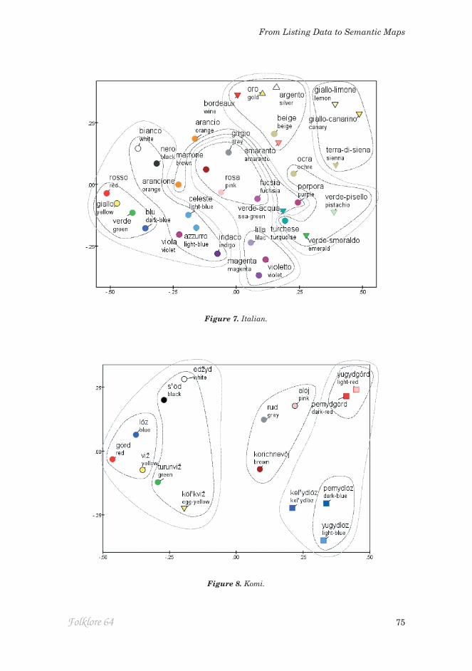
In Komi-Zyrian the initial gradient of putative BCTs extends for eight terms, the eighth being rud ‘grey’, followed by a step to the modified ‘blue’ forms kelyd’löz and pemydlöz. Subsequently alöj ‘pink’ and koričnevöj ‘brown’ appear, neither evidently salient (the latter is a loan-word from Russian); oranževöj ‘orange’ is 25th in order of salience and not in wide use.

In Udmurt the BCT gradient extends for 11 terms. It includes lemlet ‘pink’, but ljölj – its counterpart in Southern dialects – falls along the steeper decline to the non-basic segment of the plot. The next non-basic term is busir’ ‘purple’. The ninth and tenth basic terms are nap-čuž ‘orange’ and purys’ ‘grey’, while the 11th is the ostensibly basic čagyr ‘light blue’.

Languages like Udmurt, in which more than one BCT share the region of colour space spanned by the English BCT ‘blue’, are of special interest because of the challenge they pose to the dogma that the ceiling of complexity is set at 11 BCTs. The canonical case is Russian, where multiple lines of inquiry converge in supporting the basicness of goluboj ‘light blue’ (Paramei 2005, 2007). In Figure 1(j) it is the eighth most salient term. Lithuanian is a second candidate: like Udmurt, there has been linguistic pressure from neighbouring Russian-speaking populations, perhaps contributing to the basicness of the ‘light-blue’ term žydra. Figure 1(i) ranks žydra as the 11th most salient term, at the beginning of the step from BCTs down to non-basic terms, ahead of salotinė ‘light green’. In Italian the two light-blue terms azzurro and celeste are the 11th and 12th most salient terms, ahead of grigio ‘grey’, which is followed by an abrupt drop in salience to fucsia ‘fuchsia’. In contrast, in Turkish it is the dark-blue term lacivert that may be basic (Özgen & Davies 1998), complement-ing the broader ‘blue’ term mavi. The status of lacivert remains moot (Rätsep 2011) but it is the 11th most salient term in Figure 1(n), again ahead of ‘grey’ gri, attesting to its.

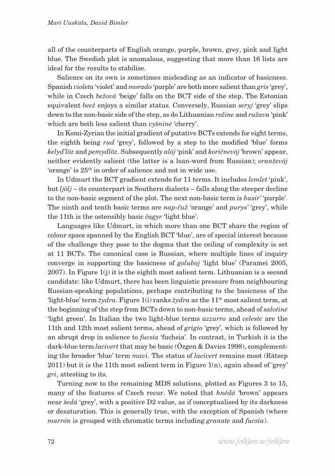
Turning now to the remaining MDS solutions, plotted as Figures 3 to 15, many of the features of Czech recur. We noted that hnědá ‘brown’ appears near šedá ‘grey’, with a positive D2 value, as if conceptualised by its darkness or desaturation. This is generally true, with the exception of Spanish (where marrón is grouped with chromatic terms including granate and fucsia).

Folklore 64 73


Figure 3. English.

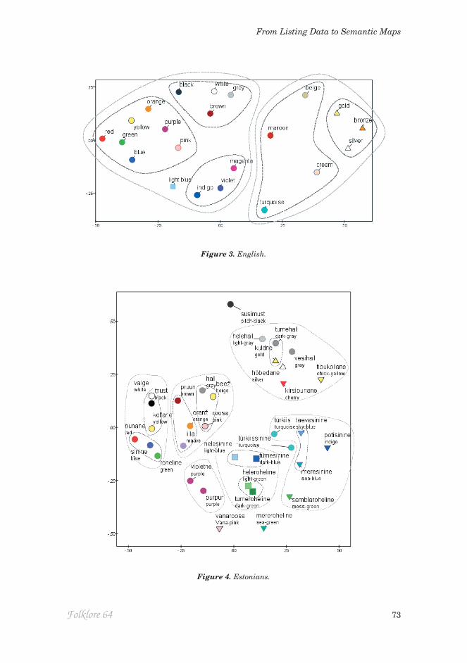
Figure 4. Estonians.



Figure 5. Finnish.

Figure 6. Hungarian.

Folklore 64 75


Figure 7. Italian.

Figure 8. Komi.



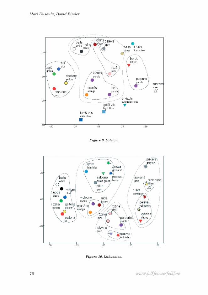
Figure 9. Latvian.

Figure 10. Lithuanian.

Folklore 64 77


Figure 11. Russian.

Figure 12. Spanish.



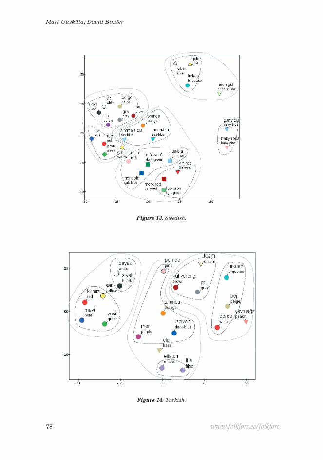
Figure 13. Swedish.

Figure 14. Turkish.

Folklore 64 79


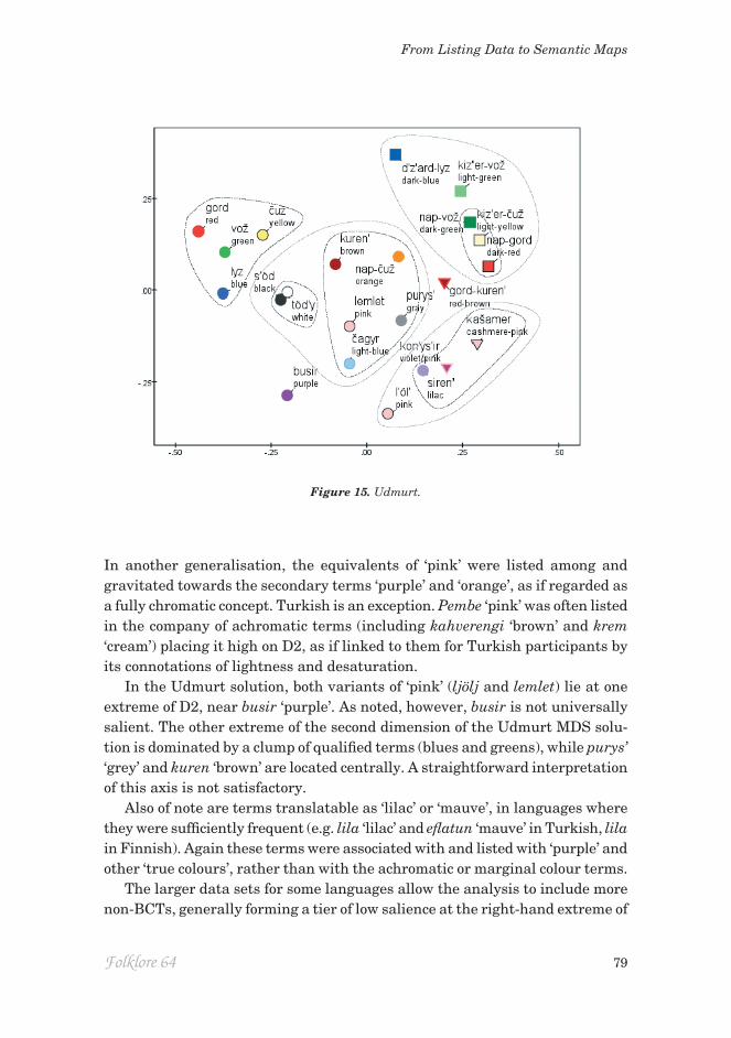
In another generalisation, the equivalents of ‘pink’ were listed among and gravitated towards the secondary terms ‘purple’ and ‘orange’, as if regarded as a fully chromatic concept. Turkish is an exception. Pembe ‘pink’ was often listed in the company of achromatic terms (including kahverengi ‘brown’ and krem ‘cream’) placing it high on D2, as if linked to them for Turkish participants by its connotations of lightness and desaturation.

In the Udmurt solution, both variants of ‘pink’ (ljölj and lemlet) lie at one extreme of D2, near busir ‘purple’. As noted, however, busir is not universally salient. The other extreme of the second dimension of the Udmurt MDS solu-tion is dominated by a clump of qualified terms (blues and greens), while purys’ ‘grey’ and kuren ‘brown’ are located centrally. A straightforward interpretation of this axis is not satisfactory.

Also of note are terms translatable as ‘lilac’ or ‘mauve’, in languages where they were sufficiently frequent (e.g. lila ‘lilac’ and eflatun ‘mauve’ in Turkish, lila in Finnish). Again these terms were associated with and listed with ‘purple’ and other ‘true colours’, rather than with the achromatic or marginal colour terms.

The larger data sets for some languages allow the analysis to include more non-BCTs, generally forming a tier of low salience at the right-hand extreme of

Figure 15. Udmurt.



D1 in the MDS solutions. Note that D1 is best interpreted as the ‘priority’ aspect of salience, rather than as ‘frequency’. A term can be relatively infrequently used, but still lie to the left of D1, if those people who do list it, do so early in their lists, in the context of high-salience terms. This is most apparent for terms for which alternative forms or dialect variants exist, with participants listing only one or the other form, but in similar contexts – resulting in adjacent points in the MDS solution. Thus the Lithuanian participants are split between rožine and ružava ‘pink’, reducing the frequency of both forms, but both are high-priority (it is possible that neither word is basic; see Pranaitytė 2011). Other examples are beige and beessi ‘beige’ in Finnish, türkiis and türkiissinine ‘turquoise’ in Estonian, and in Italian arancione and arancio ‘orange’, where less than a sixth of participants used the latter truncated form. The Finnish BCT counterpart to ‘pink’ is vaalean-punainen, literally ‘light red’, although conceptually understood as a whole (Uusküla 2007). Pinkki was only listed by 16 of 68 participants, but those 16 tended to list it just before or after vaalean-punainen, testifying to its near‑synonymity and providing it with a high priority (for finer distinctions within ‘pink’ in Germanic languages, see Vejdemo et al. 2015).

Returning to less-salient terms, in the Uralic languages these tend to be ‘transparent’ terms coined by combining BCTs (e.g. ‘red-brown’), or by modify-ing them with a qualifier of lightness or saturation (‘light green’, ‘dark blue’) or a metaphorical reference (e.g. ‘sea-green’), including the dyeing process in the case of Estonian potisinine ‘indigo’, literally ‘pot‑blue’. The modified terms coalesce in distinct domains within the MDS maps, each domain grouped by a common source BCT (rather than by a common modifier). Typically in the data these terms are listed in chunks: a systematic attempt to exhaust all variants of (say) ‘blue’ before moving on to (say) ‘green’. In addition, the MDS maps suggest that the sequence of these sub-lists tends to echo the earlier sequence of the BCTs themselves, for the arrangement of these domains is similar (though on a larger scale) to the arrangement of the BCTs in the ‘basic’ region of the map (for instance, tume-hall ‘dark grey’ and other modified greys in the Estonian map receive high D2 coordinates that locate them close to kuldne ‘gold’, echoing the role of D2 in distinguishing hall ‘grey’ itself from chromatic secondary BCTs). Typically ‘green’ and ‘blue’ are particularly generative, and the derived forms are characterised by their chromatic content, judging from their extreme positions on the D2 axis (see Figures 4, 6, 8; also Latvian and Swedish, Figures 9 and 13).

Figure 10 for Lithuanian displays a similar peripheral fringe of ‘nuance’ terms such as žalsva ‘greenish’. The morphology of Lithuanian promotes the formation and the acceptance of such terms (Pranaitytė 2011). In contrast, in English hedged terms of the form ‘X-ish’ are valid descriptions for non-proto-typal examples of a colour, but they are seldom regarded as colours per se, and Smith, Furbee, Maynard, Quick and Ross (1995) reported the form to be rare

Folklore 64 81


across the 353 lists they elicited. Žalsva and melsva ‘bluish’ were linked with desaturated concepts.

This leads us to terms cognate with ‘turquoise’, which were salient in many languages. They reveal an interesting dichotomy in the way it is conceptualised. In Estonian, türkiis ‘turquoise’ and türkiis-sinine ‘turquoise-blue’ both belong to the cluster of qualified blues. This also occurs for Hungarian türkiz-kék. In Italian, turchese is located within a sector of qualified greens with verde acqua ‘sea-green’ and verde smeraldo ‘emerald green’ as its closest neighbours (while Russian birjuzovyj is clustered with a pair of ‘lilac’ descriptors). How-ever, the Latvian data treated tirkīzzils ‘turquoise blue’ as a different colour from tirkīz ‘turquoise’: the former, regarded as a qualified ‘blue’, is located near gaiši zils ‘dark blue’, while the latter is at the opposite extreme of D2, near bēšs ‘beige’. Similarly, Turkish turkuaz, Spanish turquesa, Swedish turkos, Finnish turkoosi and Czech tyrkysová are in the neighbourhood of ‘beige’ or ‘grey’ or the metallic sheens.

Equivalents of ‘beige’ were surprisingly salient in the listing data for several languages, e.g. bész (Hungarian) and bej (Turkish). Hungarian also possesses drapp, with a similar denotation as bész (Eessalu & Uusküla 2013). Participants seemed to focus on the non-chromatic connotations of the concept, associating and listing these terms with ‘grey’, or with ‘gold’ and ‘silver’ when the metallic sheens were listed.

Finally we return to the ‘secondary blue’ terms that complement the ‘primary blue’ in some languages. For Turkish, the MDS solution shows mavi ‘blue’ in the usual group of ‘cardinal hues’, while lacivert ‘dark blue’ was listed with the other chromatic secondary terms mor ‘purple’ and turuncu ‘orange’. In Italian, a similar relationship emerged between the more inclusive primary term blu, and azzurro and celeste ‘light blue’, both mapped between viola ‘violet’ and rosa ‘pink’. Of those two, celeste has stronger connotations of lightness and desatu-ration, and it was slightly closer to grey. The Udmurt term čagyr ‘light blue’ behaves similarly. In contrast, žydra in Lithuanian appeared as a desaturated concept in the data, associated with pilka ‘grey’, salotinė ‘light green’, and the nuanced terms žalsva and melsva, ‘greenish’ and ‘bluish’.

Turning to Russian listings, the present results are aberrant in several re-spects. Data were sparse in this sample, with 24 participants recruited. Five of those 24 treated the cardinal hues and chromatic secondary terms together as a distinct ‘chunk’, listing them in a recurring rainbow sequence from krasnyj ‘red’ to fioletovyj ‘purple’. The same pattern emerges in listing data from L1 Russian speakers in Estonia (Rätsep, pers. comm.). Presumably this reflects Russian pedagogy, which instils the colours of the rainbow with a suitable mnemonic, much as English-speaking children learn colour terms in a rainbow sequence with the ROYGBIV acronym (Paramei, pers. comm.). The consensus



across these five participants prevailed over the less‑structured responses from the other 19 and distorted the location of terms in the MDS solution to accom-modate a distinct band of rainbow terms, separated from other clusters of hues by large gaps (the mnemonic lists goluboj between zelenyj ‘green’ and sinij, but in the map its neighbours are sinij and fioletovyj).

DISCUSSION

Comparisons can be drawn with the semantic domain of animal names as a precedent, where the analysis of listing data to obtain a spatial map is long-established. The first dimension of such maps is often a gradient of familiar-ity or typicality, compatible with the frequency ranking reported by Henley (1969) – which started with ‘dog, lion, cat, horse, tiger’ and proceeded to less over-learned animals – or by Borgatti (1999) which began ‘cat, dog, elephant, zebra…’ A second dimension often makes a conceptual distinction between domestic and wild animals – the former category encompassing pets and farm animals, and the latter encompassing pests as well as ‘zoo animals’ (Shepard 1974).

Paulsen, Romero, Chan, Davis, Heaton and Jeste (1996) pooled the data of schizophrenic subjects to derive a map of animal name semantics, and drew conclusions from the differences between that map and one derived from normal controls (see also Aloia et al. 1996). That is, instead of assuming that all English speakers share a consensus animal-name semantic network – the assumption used here for colour terms – they allowed for the possibility of more than one consensus. The homogeneity of a group of subjects is a question of the agree-ment among their adjacency matrices SEPp. After reducing individual listings to adjacencies, the range of variation among them can be studied with factor analysis, although that line of inquiry is not pursued here.

In a special case of individual variation, it has been reported that women perform better than men at colour-related cognitive and perceptual tasks. In particular, they access a larger vocabulary when describing hue samples (Mylonas & Paramei & MacDonald 2014); these reports are not restricted to English-speaking samples (Rätsep 2013; Ryabina 2009). We therefore expected to find a gender difference in the number of terms each participant listed. The difference was indeed significant overall, but interestingly it varied significantly between samples, reaching the threshold of significance for only five languages in isolation, with some samples showing no difference at all. It is conceivable that men and women also differ in their patterns of listing, accessing different male and female consensus semantic networks. That possibility lies outside the scope of this study.

Folklore 64 83


The list-based derivation of dissimilarity or adjacency used here is not the only possibility. It is essentially the same as Friendly’s (1977) definition, except that ADJ(i,j) is the geometric rather than the arithmetic mean of list-wise rank-ing differences, resulting from the log transform of those ranking differences. This transform ensures a degree of diminishing returns in the definition: the presence of a term between terms A and B in a list indicates a higher dissimi-larity than if A and B were consecutive; the presence of two interposed terms shows the dissimilarity to be higher again, but the increment in dissimilarity is smaller.

Borgatti (1999) used the list co-occurrences cij as a simple estimate of inter-item proximity, unweighted by the relative position of the i-th and j-th terms in each list. This is equivalent to assuming that once a term has been listed and the node representing it in the semantic network has been activated, it remains activated throughout the list, continuing to prime the nodes to which it is linked and raising the likelihood that they will also be listed. This analysis is dominated, however, by the frequency of each term in isolation: Borgatti’s MDS solutions were centred on a core of prototypal, often-listed members of the domain in question, surrounded like the yolk of a fried egg by a halo of progres-sively less-salient members, frequency becoming a radial gradient while other axes were uninterpretable. At the other extreme one could assume that activa-tion declines very rapidly with time, and include only direct adjacency in the calculation of similarity, accruing a point towards the association of two terms only if they appear consecutively in a list. However, this results in sparse data.

Henley’s (1969) definition normalised ranking differences by the length of each list (Chan et al. 1993 and Aloia et al. 1996 also used normalising terms; also Prescott et al. 2006). Finally, in one extension of multidimensional scal-ing, the N points within a spatial model are adjusted to match ‘three-way dis-similarities’, which describe the relatedness of three items at a time, and are stored in a N-by-N-by-N matrix (e.g. Cox & Cox & Branca 1991). Definitions of list-based dissimilarity easily generalise to this approach.

Dissimilarities can also be obtained from text corpora by treating them as simple lists of words and calculating the lexical co-occurrence between pairs of words (Goñi et al. 2011; Lund & Burgess 1996).

CONCLUSIONS

Previous studies of colour linguistics used the listing or free-emission task as part of a standard field method for eliciting the basic colour terms in a given language (Davies & Corbett 1994a, 1994b; Sutrop 2002; Uusküla 2007; Vejdemo et al. 2015). In this context, the participants’ lists are processed to yield a sali-



ence value for each term such as CSI or Smith’s function. Listing data are also often collected in other domains of linguistic or anthropological interest such as body parts or kinship terms.

On its own, a discontinuity in the otherwise-exponential decline of CSI is not an infallible criterion of ‘basicness’. An unequivocal BCT can slip down the rankings if its appearance in lists is reduced by the weakness of the cognitive associations connecting it to other BCTs, while conversely a hyponym or reces-sive near-synonym of a BCT can be elevated into the ‘basic’ side of the step if it is strongly linked to its dominant partner (this occurs for ‘violet’ in the English language results from Smith et al. 1995). In addition, the step is not universally obvious or abrupt (Davies & Corbett 1994b); it may continue over more than one interval and leave some terms partway down the steeper incline, requir-ing a subjective judgement whether they are BCTs or not. Cognitive salience is only one indicator, to be weighed with others.

Other research traditions have adopted the listing task for other objec-tives – notably anthropology and cognitive psychology (Borgatti 1999; Weller & Romney 1988), and clinical psychiatry where it serves a diagnostic purpose as the Noun Fluency Test. These other traditions inspired us to apply multidi-mensional scaling to listing data, resulting in spatial representations of colour terms in different languages.

A spatial map is a good fit to a list if the sum of successive distances within it – following a trajectory between points in the order those terms were se-lected – is relatively low, with sequential terms being spatially adjacent. It is worth noting that MDS solutions derived from overt judgements of similarity provided a good fit, in this sense, to recalled sequences of terms (Caramazza et al. 1976; Romney et al. 1993). The process of converting lists to adjacency estimates, and applying MDS to convert those in turn into language‑specific maps, can be understood as a way of locating points to minimise this trajectory length, averaged across participants.

A recurring feature of the MDS solutions is the overall shape, reminiscent of a comet. Individual maps consist of a compact ‘head’ of first‑used, highly‑associated terms at one extreme of the ‘priority’ axis, while at the other axial extreme the lower-priority terms spread out across the second dimension. This shape is a natural outcome of listing behaviour. By definition, highly‑salient terms all appear near the start of the lists, limiting the differences among their ranks. Conversely, less-salient terms can appear anywhere in a list, which allows larger ranking differences among them and requires more spread along the second axis. When Corbett and Davies (1997, Figure 9.2) used Correspondence Analysis to compare a range of different behavioural and text-based measures of basicness, they found that English colour terms were spread out across a similar geometrical ‘map’: salience was one axis, while a second axis expressed

Folklore 64 85


secondary differences. In an attempt to eliminate ‘salience’ as a confounding factor in their calculation of list-based similarity, Aloia, Gourovitch, Weinberger and Goldberg (1996) and Chan, Butters, Paulsen, Salmon, Swenson and Maloney (1993) included terms to weight each subject’s contribution. We feel it is easier to allow salience to emerge as its own separable dimension.

The second dimension captures a distinction between prototypal terms of ‘real colour’ and unchromatic, marginal or ‘second-class’ terms. Among primary basic terms, it separates ‘black’ and ‘white’ from the cardinal hues; ‘grey’ and often ‘pink’ and ‘brown’ from chromatic secondary terms; while among the non-basic terms it distinguishes the metallic sheens ‘gold’ and ‘silver’ from chromatic hyponyms like ‘mauve’. A participant’s chain of associations might jump between more- and less-basic chromatic terms, or between desaturated concepts.

For languages with sufficient data to include larger numbers of terms in the analysis – modified basics, or metonyms – the picture is complicated when these are inserted into two-dimensional maps (often as clumps of points, grouped together by common derivation from the same basic term). It may be that three-dimensional MDS solutions would reveal other cross-cultural commonalities.

Recent attention has turned beyond the inner circle of BCTs, to terms in common but not universal use (which might potentially become basic if the need for colour communication within a culture places enough emphasis on specificity) (Mylonas & MacDonald 2016; Lindsey & Brown 2014; Jraissati et al. 2012). Turquoise and German türkis have been mentioned as a possible incipient BCT (Zollinger 1984). However, a recent survey of American English (Lindsey & Brown 2014) found ‘teal’ to be the more common term for blue-green stimuli. The trend here, though with exceptions, was for ‘turquoise’ cognate terms to be linked with metallic sheens, suggesting that the concept is dominated by its non-chromatic aspects (perhaps emphasising the function of turquoise as a semi-precious component in jewellery).

In another example, Eessalu and Uusküla (2013) noted the relatively high salience of the equivalents of ‘beige’ in many of the present data sets; terms like Turkish bej and Hungarian bézs (also present in Hungarian as drapp). Again, these terms were coupled with achromatic terms such as ‘grey’, suggesting that the concept is not a chromatic one: ‘beige’ being an absence of decisive colour. In English, ‘beige’ does not feature among the 21 most salient terms in Smith, Furbee, Maynard, Quick, and Ross (1995). Sturges and Whitfield (1995) found ‘beige’ to be one of the three most frequent non-basic English terms for colour naming – the other two being ‘cream’ and ‘turquoise’ – and noted its value for identifying hues in a region of colour space that is poorly served by the 11 BCTs, and remote from their foci. The prominence of the term is a recent phenomenon: in a similar study eight years earlier (Boynton & Olson 1987), the use of ‘beige’ showed little consistency or popularity.



Distinctions among BCTs are also of interest. It seems natural to distin-guish the four ‘cardinal’ terms plus white and black as ‘primary’ terms, and to regard the remaining BCTs as secondary: each derived from two primaries, combining them or occupying the borderland between them (Kay & McDaniel 1978). Some measures of basicness support this intuition, but not all (Corbett & Davies 1997; Sturges & Whitfield 1995). Many of the present CSI plots and MDS solutions display a gap between the primary and derived BCTs.

In several of the languages studied here, the sector of colour space covered by the English category ‘blue’ is split between a ‘primary blue’ term and a com-plementary ‘secondary blue’, both basic, though the level of lightness separating the two categories is not necessarily the same in each language. In Italian, for instance, azzurro and celeste ‘light blue’ are both candidates for basic status, although they are less inclusive than blu ‘blue’ or ‘dark blue’ (Paramei & Me-negaz 2013; Bimler & Uusküla 2014). Lithuanian and Udmurt are two more examples, with ‘light blue’ terms žydra and čagyr respectively; contact with Russian may have encouraged their emergence (several strands of evidence support the basicness of žydra: Bimler & Uusküla, in preparation). In the present results, the secondary terms azzurro, celeste, Udmurt čagyr ‘light blue’ and Turkish lacivert ‘dark blue’ were all treated as chromatic concepts, while in contrast Lithuanian žydra ‘light blue’ had more in common with pilka ‘grey’.

Similarities across language‑specific MDS solutions point to a shared, cross‑cultural pattern of associations among terms, structuring the sequence in which they are listed. The ‘chunking’ of terms indicates a shared system of concep-tual attributes used to group them. In addition, dimensions of the MDS maps reflect conceptual themes at a higher level of abstraction. Note that this is not simply a consequence of the familiar cross-cultural regularities in the way that BCTs partition colour space into categories, and in the centroids and focal hues of these categories (i.e. the denotational use of the terms). This follows from the divergence between the maps and the spatial maps obtained when people rate the perceptual similarities among colour terms (from observation or from memory): listing associations access a more abstract aspect of ‘similarity’. Perceptual opposites may be closely related at the conceptual level (‘black’ and ‘white’, ‘purple’ and ‘orange’).

ACKNOWLEDGEMENTS

Some of these data and versions of diagrams were previously reported to the Gruppo del Colore meeting in Genoa.

Folklore 64 87


The whole data collection was founded by the Estonian Science Foundation grant no. 8168 (awarded to Mari Uusküla) and Estonian Ministry of Educa-tion and Research project no. SF0050037s10 (awarded to Urmas Sutrop). The authors are thankful to all data collectors.

REFERENCES

Aloia, Mark S. & Gourovitch, Monica L. & Weinberger, Daniel R. & Goldberg, Terry E. 1996. An Investigation of Semantic Space in Patients with Schizophrenia. Journal of International Neuropsychological Society, Vol. 2, No. 4, pp. 267–273. http://dx.doi.org/10.1017/S1355617700001272.

Berlin, Brent & Kay, Paul 1991 [1969]. Basic Color Terms: Their Universality and Evolution. Berkeley & Los Angeles & Oxford: University of California Press.

Bimler, David & Uusküla, Mari 2014. “Clothed in Triple Blues”: Sorting Out the Italian Blues. Journal of the Optical Society of America, Vol. 31, No. 4, pp. A332–A340. http://dx.doi.org/10.1364/JOSAA.31.00A332.

Borgatti, Stephen P. 1999. Elicitation Techniques for Cultural Domain Analysis. In: J. Schensul & M. D. LeCompte (eds.) Ethnographer’s Toolkit, Vol. 3. Walnut Creek: AltaMira Press, pp. 115–151.

Boynton, Robert M. & Conrad X. Olson 1987. Locating Basic Colors in the OSA Space. Color Research & Application, Vol. 12, No. 2, pp. 94–105. http://dx.doi.org/10.1002/col.5080120209.

Caramazza, Alfonso & Hersh, Harry & Torgerson, Warren S. 1976. Subjective Structures and Operations in Semantic Memory. Journal of Verbal Learning and Verbal Behavior, Vol. 15, No. 1, pp. 103–117. http://dx.doi.org/10.1016/S0022-5371(76)90011-6.

Chan, Agnes S. & Butters, Nelson & Paulsen, Jane S. & Salmon, David P. & Swenson, Michael R. & Maloney, Laurence T. 1993. An Assessment of the Semantic Net-work in Patients with Alzheimer’s Disease. Journal of Cognitive Neuroscience, Vol. 5, No. 2, pp. 254–261. doi:10.1162/jocn.1993.5.2.254.

Collins, Allan M. & Loftus, Elizabeth F. 1975. A Spreading-Activation Theory of Semantic Processing. Psychological Review, Vol. 82, No. 6, pp. 407–428. http://dx.doi.org/10.1037/0033-295X.82.6.407.

Corbett, Greville C. & Davies, Ian R. L. 1997. Establishing Basic Color Terms: Measures and Techniques. In: C. L. Hardin & L. Maffi (eds.) Color Categories in Thought and Language. Cambridge: Cambridge University Press, pp. 197–223.

Cox, Trevor F. & Cox, Michael A. A. & Branco, Joao A. 1991. Multidimensional Scaling for n-Tuples. British Journal of Mathematical & Statistical Psychology, Vol. 44, No. 1, pp. 195–206. http://dx.doi.org/10.1111/j.2044-8317.1991.tb00955.x.

Davies, Ian R. L. & Corbett, Greville C. 1994a. A Statistical Approach to Determining Basic Color Terms: An Account of Xhosa. Journal of Linguistic Anthropology, Vol. 4, No. 2, pp. 175–193. http://dx.doi.org/10.1525/jlin.1994.4.2.175.

Davies, Ian R. L. & Corbett, Greville C. 1994b. The Basic Color Terms of Russian. Linguistics, Vol. 32, No. 1, pp. 65–89. http://dx.doi.org/10.1515/ling.1994.32.1.65.



Davies, Ian R. L. & Corbett, Greville C. & Margalef, José Bayo 1995. Colour Terms in Catalan: An Investigation of Eighty Informants, Concentrating on the Purple and Blue Regions. Transactions of the Philological Society, Vol. 93, No. 1, pp. 17–49. http://dx.doi.org/10.1111/j.1467-968X.1995.tb00435.x.

Eessalu, Martin & Uusküla, Mari 2013.The Special Case of Beige: A Cross-Linguistic Study. In: M. Rossi (ed.) Colour and Colorimetry: Multidisciplinary Contributions, Vol. IXB. Maggioli: Rimini, pp. 168–176. Available at https://www.researchgate.net/publication/264461470_The_special_case_of_beige_A_cross-linguistic_study, last accessed on May 20, 2016.

Fletcher, Robert 1980. The City University Colour Vision Test. 2nd ed. London: Keeler.Friendly, Michael L. 1977. In Search of the M-Gram: The Structure of Organization

in Free Recall. Cognitive Psychology, Vol. 9, No. 2, pp. 188–249. http://dx.doi.org/10.1016/0010-0285(77)90008-1.

Friendly, Michael L. 1979. Methods for Finding Graphic Representations of Associative Memory Structures. In: C. R. Puff (ed.) Memory Organization and Structure. New York: Academic Press, pp. 85–129.

Goñi, J. & Arrondo, G. & Sepulcre, J. & Martincorena, I. & Vélez de Mendizabal, N. & Corominas-Murtra, B. & Bejarano, B. & Ardanza-Trevijano, S. & Peraita, H. & Wall, D. P. & Villoslada, P. 2011. The Semantic Organization of the Animal Category: Evidence from Semantic Verbal Fluency and Network Theory. Cogni-tive Processing, Vol. 12, No. 2, pp. 183–196. DOI: 10.1007/s10339-010-0372-x.

Harkness, Sarah 1973. Universal Aspects of Learning Color Codes: A Study in Two Cultures. Ethos, Vol. 1, No. 2, pp. 175–200. DOI: 10.1525/eth.1973.1.2.02a00030.

Henley, Nancy M. 1969. A Psychological Study of the Semantics of Animal Terms. Jour-nal of Verbal Learning and Verbal Behavior, Vol. 8, No. 2, pp. 176–184. http://dx.doi.org/10.1016/S0022-5371(69)80058-7.

Hippisley, Andrew R. 2001. Basic blue in East Slavonic. Linguistics, Vol. 39, No. 1, pp. 151–179. http://dx.doi.org/10.1515/ling.2001.003.

Ishihara, Shinobu 2008. Ishihara’s Tests for Colour Deficiency. 24 Plates Edition. Tokyo: Kanehara Trading Inc.

Jraissati, Yasmina & Wakui, Elley & Decock, Lieven & Douven, Igor 2012. Constraints on Colour Category Formation. International Studies in the Philosophy of Science, Vol. 26, No. 2, pp. 171–196. http://dx.doi.org/10.1080/02698595.2012.703479.

Kay, Paul & McDaniel, Chad K. 1978. The Linguistic Significance of the Meanings of Basic Color Terms. Language, Vol. 54, No. 3, pp. 610–646. http://dx.doi.org/10.1353/lan.1978.0035.

Kerttula, Seija 2007. Relative Basicness of Color Terms: Modeling and Measurement. In: Robert E. MacLaury & Galina V. Paramei & Don Dedrick (eds.) Anthropol-ogy of Color. Amsterdam & Philadelphia: John Benjamins Publishing Company, pp. 151–169. DOI: 10.1075/z.137.11ker.

Lindsey, Delwin T. & Brown, Angela M. 2014. The Color Lexicon of American English. Journal of Vision, Vol. 14, No. 2, pp. 1–25. http://dx.doi.org/10.1167/14.2.17.

Lund, Kevin & Burgess, Curt 1996. Producing High-Dimensional Semantic Spaces from Lexical Co-Occurrence. Behavior Research Methods, Instruments, & Computers, Vol. 28, No. 2, pp. 203–208. http://dx.doi.org/10.3758/BF03204766.

Mylonas, Dimitris & MacDonald, Lindsay 2016. Augmenting Basic Colour Terms in English. Color Research & Application, Vol. 41, No. 1, pp. 32–42. http://dx.doi.org/10.1002/col.21944.

Folklore 64 89


Mylonas, Dimitris & Paramei, Galina V. & MacDonald, Lindsay 2014. Gender Dif-ferences in Colour Naming. In: Wendy Anderson & Carole P. Biggam & Car-ole Hough & Christian Kay (eds.) Colour Studies: A Broad Spectrum. Amster-dam & Philadelphia: John Benjamins Publishing Company, pp. 225–239. DOI: 10.1075/z.191.15myl.

Özgen, Emre & Davies, Ian R. L. 1998. Turkish Color Terms: Tests of Berlin and Kay’s Theory of Color Universals and Linguistic Relativity. Linguistics, Vol. 36, No. 5, pp. 919–956. http://dx.doi.org/10.1515/ling.1998.36.5.919.

Paramei, Galina V. 2005. Singing the Russian Blues: An Argument for Culturally Basic Color Terms. Cross-Cultural Research, Vol. 39, No. 1, pp. 10–38. http://dx.doi.org/10.1177/1069397104267888.

Paramei, Galina V. 2007. Russian ‘Blues’: Controversies of Basicness. In: Robert E. MacLaury & Galina V. Paramei & Don Dedrick (eds.) Anthropology of Color. Amsterdam & Philadelphia: John Benjamins Publishing Company, pp. 75–106. DOI: 10.1075/z.137.07par.

Paramei, Galina V. & Menegaz, Gloria 2013.‘Italian Blues’: A Challenge to the Universal Inventory of Basic Colour Terms. In: Maurizio Rossi (ed.) Colour and Colorimetry: Multidisciplinary Contributions, Vol. IX B, pp. 164–167. Rimini: Maggioli S.p.A.

Paulsen, Jane S. & Romero, Ramon & Chan, Agnes & Davis, Amy V. & Heaton, Robert K. & Jeste, Dilip V. 1996. Impairment of the Semantic Network in Schizophrenia. Psychiatry Research, Vol. 63, No. 2–3, pp. 109–121. http://dx.doi.org/10.1016/0165-1781(96)02901-0.

Pranaitytė, Simona 2011. Põhivärvinimed leedu keeles. [The Basic Colour Terms of Lithuanian.] In: Mari Uusküla & Urmas Sutrop (eds.) Värvinimede raamat. [A Book of Colour Terms.] Tallinn: Eesti Keele Sihtasutus, pp. 271–300. Avail-able at http://www.academia.edu/23710383/V%C3%A4rvinimede_raamat, last accessed on May 23, 2016.

Prescott, Tony J. & Newton, Lisa D. & Mir, Nusrat U. & Woodruff, Peter W. R. & Parks, Randolf W. 2006. A New Dissimilarity Measure for Finding Semantic Structure in Category Fluency Data with Implications for Understanding Memory Organiza-tion in Schizophrenia. Neuropsychology, Vol. 20, No. 6, pp. 685–699. http://dx.doi.org/10.1037/0894-4105.20.6.685.

Rätsep, Kaidi 2011. Preliminary Research on Turkish Basic Colour Terms with an Emphasis on Blue. In: C. P. Biggam & C. A. Hough & C. J. Kay & D. R. Sim-mons (eds.) New Directions in Colour Studies. Amsterdam & Philadelphia: John Benjamins Publishing Company, pp. 133−145.

Rätsep, Kaidi 2013. Some Remarks on Gender Differences in Turkish Colour Vocabulary. In: Balázs Surányi (ed.) Proceedings of the Second Central European Conference in Linguistics for Postgraduate Students. Second Central European Conference in Linguistics for Postgraduate Students (CECIL’S 2), Pázmány Péter Catholic University, Piliscsaba, Hungary, on 24–25 August 2012. Budapest: Pázmány Péter Catholic University, pp. 219−229.

Regier, Terry & Kay, Paul & Cook, Richard S. 2005. Universal Foci and Varying Bounda-ries in Linguistic Color Categories. In: Bruno G. Bara & Lawrence Barsalou & Monica Bucciarelli (eds.) Proceedings of the 27th Annual Conference of the Cog-nitive Science Society (CogSci 2005), July 21–23, Stresa, Italy, pp. 1827–1832. Available at http://csjarchive.cogsci.rpi.edu/proceedings/2005/docs/p1827.pdf, last accessed on May 23, 2016.


www.folklore.ee/folklore

Roberson, Debi & Davidoff, Jules & Davies, Ian R. L. & Shapiro, Laura R. 2004. The De-velopment of Color Categories in Two Languages: A Longitudinal Study. Journal of Experimental Psychology: General, Vol. 133, No. 4, pp. 554–571. http://dx.doi.org/10.1037/0096-3445.133.4.554.

Romney, A. Kimball & Brewer, Devon D. & Batchelder, William H. 1993. Predicting Clus-tering from Semantic Structure. Psychological Science, Vol. 4, No. 1, pp. 28–34. http://dx.doi.org/10.1111/j.1467-9280.1993.tb00552.x.

Ryabina, Elena 2009. Sex-Related Differences in the Colour Vocabulary of Udmurts. WEBFU: Wiener elektronische Beiträge des Instituts für Finno-Ugristik. Available at http://www.univie.ac.at/webfu/texte/12Ryabina.pdf, last accessed on May 23, 2016.

Ryabina, Elena 2011. Differences in the Distribution of Colour Terms in Colour Space in the Russian, Udmurt and Komi Languages. ESUKA-JEFUL, Vol. 2, No. 2, pp. 191–213. Available at http://jeful.ut.ee/public/files/Ryabina%20191‑213.pdf, last accessed on May 23, 2016.

Shepard, Roger N. 1974. Representation of Structure in Similarity Data: Problems and Prospects. Psychometrika, Vol. 39, No. 4, pp. 373–421. http://dx.doi.org/10.1007/BF02291665.

Smith, J. Jerome 1993. Using ANTHROPAC 3.5 and a Spreadsheet to Compute a Free-List Salience Index. Field Methods, Vol. 5, No. 3, pp. 1–3. doi:10.1177/1525822X9300500301.

Smith, J. Jerome & Furbee, Louanna & Maynard, Kelly & Quick, Sarah & Ross, Larry 1995. Salience Counts: A Domain Analysis of English Color Terms. Journal of Linguistic Anthropology, Vol. 5, No. 2, pp. 203–216. http://dx.doi.org/10.1525/jlin.1995.5.2.203.

Storm, Christine 1980. The Semantic Structure of Animal Terms: A Developmental Study. International Journal of Behavioral Development, Vol. 3, No. 4, pp. 381–407. http://dx.doi.org/10.1177/016502548000300403.

Sturges, Julia & Whitfield, T. W. Allan 1995. Locating Basic Colours in the Munsell Space. Color Research and Application, Vol. 20, No. 6, pp. 364–376. http://dx.doi.org/10.1002/col.5080200605.

Sutrop, Urmas 2001. List Task and a Cognitive Salience Index. Field Methods, Vol. 13, No. 3, pp. 263–276. http://dx.doi.org/10.1177/1525822X0101300303.

Sutrop, Urmas 2002. The Vocabulary of Sense Perception in Estonian: Structure and History. Frankfurt am Main & Berlin & Bern & Bruxelles & New York & Oxford: Peter Lang.

Uusküla, Mari 2007. The Basic Colour Terms of Finnish. SKY Journal of Linguistics 20, pp. 367–397. Available at http://www.linguistics.fi/julkaisut/sky2007.shtml, last accessed on May 23, 2016.

Vejdemo, Susanne & Levisen, Carsten & van Scherpenberg, Cornelia & Beck, þórhalla Guðmundsdóttir & Næss, Åshild & Zimmermann, Martina & Stockall, Linnaea & Whelpton, Matthew 2015. Two Kinds of Pink: Development and Difference in Germanic Colour Semantics. Language Sciences, Vol. 49, pp. 19–34. http://dx.doi.org/10.1016/j.langsci.2014.07.007.

Weller, Susan C. & Romney, A. Kimball 1988. Systematic Data Collection. Newbury Park & London & New Delhi: SAGE publications.

Zollinger, Heinrich 1984. Why Just Turquoise? Remarks on the Evolution of Color Terms. Psychological Research, Vol. 46, No. 4, pp. 403–409. http://dx.doi.org/10.1007/BF00309072.

from listing data to semantic maps: cross … · cross-linguistic commonalities in cognitive...

Documents