from national accounts to macro-economic decision models

1

FROM NATIONAL ACCOUNTS TO MACRO-ECONOMIC DECISION MODELS

by Ragnar Frisch

I. INTRODUCTION

THE main objects of this paper are: (1) to present certain considerations of a general nature on the

present status of economic theory as a tool for economic policy. (2) to point out how fundamentally important in this connec-

tion is work on national income and wealth and to suggest general principles for the way in which material contained in national accounts may be organized and reshaped so as to be most useful for the application of economic theory to problems of economic policy. This leads to the concept of a decision model and to a special technique for handling such models.

(3) finally to give, by way of example, a brief account of work that has been done along these lines in Norway.

The work there goes on in three centres: (1) The University Institute of Economics, Oslo, of which I am the Director; (2) The Central Bureau of Statistics, directed by Mr. Petter Jakob Bjerve and with Mr. Odd Aukrust as the chief of its Research Division; and (3) The National Budgets Division in the Ministry of Finance. The head of this Division is Mr. Eivind Erichsen. The Institute concentrates its efforts on the most general aspects of the problem and tries to push research in new directions. The Central Bureau of Statistics provides the solid empirical basis without which all the work would be only a game with symbols. And the National Budgets Division scrutinizes the results and sees if and how some of them may be put to practical applicatio~~. There is a wholehearted co- operation between the three centres with frequent joint research meetings and a close friendship between the research workers in the group. This ensures effective and smooth-running work. What I have to say will, of course, be colonred by the Institute's viewpoint. Other Norwegians present will be able to give further information on the work in the other centres.

Many of the ideas and viewpoints I shall bring forth are strongly influenced by what I have learned in talks and co- operative work with friends and associates of the Oslo group.

1

2 INCOME A N D WEALTH

As a matter of fact, on many points it is really impossible to find out who is responsible for what. Those who have contributed in the most active way to forming my present views include - apart from those already mentioned - Mr. Helge Seip, Chief of the Tax Research Bureau in the Central Bureau of Statistics, Mr. Per Sevaldson, Chief of the input-output unit of the Central Bureau of Statistics, Mr. Hans Heli, Assistant Professor at Oslo University and in charge of the daily supervision of the work of the research associates who work on the decision model in the University Institute. Of the research associates of the Institute, I must mention in particular Mr. Leif Johansen, who has been working under my direction on theoretical aspects of the problem. In a general way I owe much to stimulating talks with my old-time friend and colleague Professor Trygve Haavelmo.

11. THE NATURE OF DECISION MODELS

When discussing the nature of decision models it may be useful to start with a few theoretical considerations, even if they are concerned with concepts that cannot at the present time be expressed empirically in figures.

First some words about optimality in the Pareto sense. The idea of Pareto-optimality is, as you all know, derived from a model where m commodities, the quantities of which are denoted by X,. . . X,, are evaluated by n individuals numbered from 1 to n. A point is said to be Pareto-optimal if it is impossible to depart from this point without making at least one of the individuals worse off. When we use the concept of Pareto- optimality it is necessary to specify very carefully the conditions under which an optimum is to be achieved. For instance, is the optimality to be understood only subject to the condition that the point (X,. . .Xm) satisfies a certain production constraint? If so, we may say that we have Pareto-optimality under the production constraint. Or are we looking for points that are Pareto-optimal under a set of conditions that consist simultaneously of the production constraint and some sort of distribution constraint? The region of points that are Pareto- optimal under one of these sets of conditions by no means coincides with the region of points that are Pareto-optimal under other conditions. In discussing the precise relation

RAGNAR FRISCH 3

between the regions that are optimal under various sets of conditions, some rather tricky situations emerge. I have discussed some of them in a paper 'On welfare theory and Pareto regions'.

The necessity of specifying conditions when speaking of Pareto-optimal points is only a special manifestation of a basic principle underlying the whole theory of choice. The absurdities which may be produced by carelessness on this point may, perhaps, be illustrated by the following 'theoretical analysis' of the 'regime' which consists in forcing people to do abominable things under the threat of being shot. Firstly, this regime has the important property that any person subject to it is perfectly free to choose himself the alternative which he likes. Secondly, this being so, everybody will, of course, choose the alternative which gives him the highest possible satisfactioii. Thirdly, any regime which allows everybody subject to it to reach the highest possible satisfaction must be a very desirable regime for these persons. Therefore, the regime considered must be a very desirable regime for those concerned. Quod erat demo~~strandum.

I believe that the necessity of specifying conditions when speaking about Pareto-optimality is particularly important when we want to find out what is really involved in the great variety of 'proofs' that have been brought out to the effect that the regime of free competition has some sort of optimal property. I am not suggesting that all attempts at 'proving theoretically' the superiority of the regime of free competition proceed on logical lines similar to those illustrated by the above example, but I think it is fair to say that some of these attempts come dangerously close to this form of logic. Translated into economic terms: 'the regime of free competition is the best of all regimes within the class of regimes which consists of the regime of free competition'. It is even possible that Pareto himself has at one time been thinking more or less along such lines, but has at a later stage recognized the fallacy. My suspicion in this direction has been confirmed by prolonged conversations with such an eminent authority on Pareto as Professor Gustavo Del Vecchio. The essence of our conversations on this point is given in the paper quoted. Another form of fallacy in using Pareto considerations to prove the superiority of the regime of free competition consists in adopting a set of assumptions which are essentially assumptions pertaining to some highly coi~trolled

4 INCOME AND WEALTH

economy. Such is for instance the proof that, in the exchange market with given initial quantities, the point reached by letting the market find its own equilibrium, when all the individuals act as quantity adapters, is Pareto-optimal under the constraint that the initial quantities are given. Who is going to give them? Some dictator?

The unwarranted applications which have been made of the Pareto principle must not, however, make us throw it away altogether.

Correctly interpreted the principle is one of izegation, not one of ajirmation. I t states that if a point is not Pareto-optimal, then it cannot he said to be a 'good' or 'efficient' point. And this must be our conclusion regardless of how in detail we have formulated our desiderata for a 'good' or 'efficient' point. In other words the principle gives a necessary condition, it segregates a class of point to which our 'good' or 'efficient' point must belong if any such points can be determined. Since the principle only gives a necessary condition, it leaves considerable lee-way in the determination of economic policies. First Pareto-optimality has to be determined under a set of obligatory constraints, that is under constraints which it is humanly impossible to change. And within the degrees of freedom that then remain, the choice must be made by a postulate in the form of a social value judgment. This social value judgment is something which the economist as scientist and technician simply has to take as a datum. But aN the rest is within his sphere of competence. It would seem that even with the above limitation of the economist's field, there is more than enough for him to do.

Here he must apply all his resources to lay bare the consequences that may be expected by adopting a particular kind of policy. A decision model is a theoretical model supported by empirical evidence and constructed with the speci6c object in mind of discussing the probable consequences of alternative courses of action. Such a model must in several respects be rather different from the type of model usually employed. In the first place the model must be constructed in such a manner that dzyerefzt economic systems, a very free economy and also economies involving different degrees of control and different social goals, can be expressed as special cases within the model. Only by this means will it be possible to compare the results of different types of economic policy. This comparison carried out

RAGNAR FRISCH 5

quite objectively is the central point around which all analysis of decision models must gravitate.

This entails amongst other things the consequence that a decision model must contain many more degrees of freedom than the usual models. These degrees of freedoin are absorbed by the introduction of supplementary conditions that define the nature of the chosen policy.

On this point we must make a clear distinction between the selection problem and the problem of regime. In the first type of problem we ask whether there exist points that satisfy certain desiderata, namely, first the desideratum of being Pareto- optimal under a given set of obligatory constraints, and second the desideratum of satisfying some additional conditions im- posed by the policy malcers according to some sort of social value criteria. An example of such a criterion would be that the share of the national income that goes to the workers should not decrease.

In the other type of problem we ask whether it is possible to indicate a concrete regime wluch will lead to the point selected according to the above principles.

When we approach the problem in this way we are obliged to take account of the number of degrees of freedom twice. First when we discuss the selection problem. And second when we discuss the problem of regime. In both cases it is essential to make sure that we have enough and only enough degrees of freedom to answer the questions put.

Another aspect of a decision model is that it should be exhaustive in the sense of including all, or at least as many as possible, of the various repercussions within the economy. This means that we must employ models which, although crude and rough in Lheir macro-economic approximation, at least are such that practically any effect which we may think of, can be looked upon as included in one or the other of the variables that belong to the model. Furthermore an important practical requirement must be met. The model must be constructed in such a way that it is possible at many points in it to introduce supplementary considerations of a practical kind. The model should as far as possible contain specific parameters that may be evaluated from a practical viewpoint and may absorb and reflect the results of the intuition and experience of practical business- men, politicians, economic historians and others whose special

B

6 INCOME AND WEALTH

knowledge it is impossible to express exactly in a model but whose contributions we should nevertheless strive to utilize to the fullest possible extent. The subrnodel which I discussed in an article in the RPvue d'Economie Politique of 1951 had many parameters designated to absorb and express judgments of this type, for instance on the pressure towards tax evasions etc. Only if we give full attention to this aspect of the model will it be possible to make it realistic. No model, however large, will ever be able to express the idni te variety of economic lie. What it can and must do is to provide a framework which provides a place for and can explain those types of repercussion that are so interwoven and complex that without it explanation is impossible. The rest must be added more or less by intuition.

A fundamental concern must be that as many as possible of the relations of the model are of the persistent (stable, autono- mous) sort. That is to say, eachrelation must, so to speak, stand on its own feet. Itmustholdgoodnomatter whether one or more of the other relations in the model breaks down or is changed. This means that in many cases we cannot be satisfied with numerical relations determined simply by applying a multiple correlation analysis to historical data as they have emerged under a spec$c sort of regime. The relations that are the most useful ones lie much deeper down in the network of causes. Very seldom will it be possible through data obtained under a single regime to discover the fundamental things which we must know if we are to analyse in a realistic way the possible consequences that may emerge when we adopt one of several other alternative regimes. This is one reason why I think that we are iikely to obtain more substantial results by approaching the want-structure and the utility evaluations of individuals than by looking superficially at the prices and quantities that are correlated in the market.

111. THE PRESSURE COEFFICIENTS

When discussing the possible effects of ecotiomic control measures, we encounter a situation that cannot be analysed by the usual concepts of economic equilibrium analysis. Indeed, the effect of the control measures is, in many cases, to take away one or more of the assumptions that underlie this equilibrium analysis. We need a type of analysis that can express the pressure

RAGNAR FRISCH 7

which such control measures produce. It will be a pressure directed towards some sort of equilibria of the classical type. It is quite conceivable that public authoricies are willing to accept the existence of such pressures provided only that they do not go beyond certain limits. As a matter of fact in many cases it is just by allowing such pressures to reach certain magnitudes that we may be able to realize certaiiz other goals that are considered important. It is therefore extremely important that we succeed in working out the decision model in such a way as to incorporate explicitly such pressure coefficients. I shall indicate brieay how they can be incorporated in the model.

The logical principles will be explained by taking a very simple example. Suppose that we have an ordinary market where a certain good is supplied and demanded. Suppose that both sellers and buyers act as quantity adapters. That is to say if x,., is the quantity supplied and x,,, is the quantity demanded, we assume that the first of these variables is a certain function xsUp=rl~(p), that is, a function of the existing price p, and we also assume that x,,=f(p) is some other function of p. These two functions are the two ordinary supply and demand functions.

We shall assume that both these functions exist, but we shall do it in such a way as to maiiitaiiz nevertheless two degrees of

freedom. We do it by saying that these two quantities x,,, and x,,, need not be equal to the quantity x actually traded in the market. In other words we have a model with four variables and two equations, hence two degrees of freedom. To represent these two degrees of freedom we choose the variables x and p. That is to say, even if the two functions, the supply function and the demand function, are given, the market point (x,p) may fall anywhere in the diagram with p as the vertical and x as the horizontal axes. For any given position of the point (x,p) the two variables x,,, and xdcm are k e d and it is possible, indeed very natural, to compare x,., with x and also to compare xdcm with x. In other words, we can compare the existing price with the price that would have had to be realized if we had had x,,,=x or x,,=x. There exist many plausible ways of measuring the tension that exists in the market if the point (x,p) is arbitrarily given. Suppose that we define in some way or another two such coefficients Ks, and xde,,,. These coefficients will, according to the definition, be functions of (p,x). Intro-

8 INCOME AND WEALTH

ducing these functions we are still in a model with two degrees of freedom, namely now six variables and four equations. And we have a theory where we can express how the results of various possible control measures may work out. I think it is essential that our decision model is shaped in such a way as to include explicitly such pressures. That was the case with our submodel. The pressure coefficients can be handled in exactly the same way as other variables in the model. For instance when speaking of a Pareto region, this region may have pressure coefficients for some of its components.

1V. DEMAND ELASTICITIES WlTH RESPECT TO PRICE DERlVBD FROM ENGELELASTICITIES

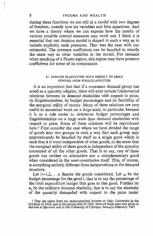
It is an important fact that if a consumer demand group has acted as a quantity adapter, there will exist certain fundamental relations between its demand elasticities with respect to price, its Engelelasticities, its budget percentages and its flexibility of the marginal utility of money. Many of these relations are very useful in numerical work on a large scale, in particular because it is as a rule easier to determine budget percentages and Engelelasticities on a large scale tthan demand elasticities with respect to price. Some of these relations will be reproduced he1e.l First consider the case where we have divided the range of goods into two groups in such a way that each group may approximately be handled by itself as a single good which is such that it is want-independent of other goods, in the sense that the marginal utility of these goods is independent of the quantity consumed of all the other goods. That is to say, one of these goods has neither an alternative nor a complementary good when considered in the want-constitution This, of course, is something entirely different from independence in the demand structure.

Let i=1,2,. . .n denote the goods considered. Let U, be the budget percentage for the good i, that is to say the percentage of the total expenditure budget that goes to this good. Further let e,, be the ordinary demand elasticity, that is to say the elasticity of the quantity demanded with respect to ihe price under

They are taken from my @meogaphed lectures at Oslo University in the fall term of 1936, and m the sprlng term of 1943. Most of them were also given in lectures at Harvard and in the University of Chicago, January-February 1947.

R A G N A R FRISCH 9

constant nominal income. Further let Ei be the Engelelasticity, that is to say, the elasticity of the quantity demanded with respect to a change in nominal income, when all the individual prices are constant. Finally let be the flexibility of the marginal utility of money for the demand group considered. If there is no quantity regulation in the market and there is no demand pressure for other reasons, we have

In other words the direct elasticity of demand can be computed by means of the budget percentage, the Engelelasticity and the flexibility of the marginal utility of money. The latter will be a common magnitude for all expenditure categories in the budget but it will, of course, depend on the type of the consumer group. Furthermore, it will depend on income.

When the direct elasticities of demand are detern~ined by (I), the crosselasticities of demand can be computed by

e. = - ,li Eiuk(1+ek3. I -E,u~ . . , . .(i+ k).

When this is done, the whole elasticity structure both with regard to prices and incomes, also the crosselasticities of demand, can be determined for the consumer group in question if the budget percentages, the Engelelasticities and the flexibility of the marginal utility of money is determined for this group.

The determination of the flexibility of the money utility for a given consumer group can be performed in different ways. One way is to select one or a few goods and make an independent determination of the direct elasticities of demand eii for the consumer group in question, without using (I), and afterwards compute the magnitude

The expression to the right in (3) ought to be the same regardless of the particular good, i, for which the direct demand elasticity has been determined, provided the income per consumption unit is the same for each individual or aggregation studied. In practice one will, of course, never obtain exactly the same value, but by making a compromise one may get a fair approxi-

10 INCOME AND WEALTH

mation to the flexibility of the marginal utility of money. Viewed in terms of the above formula, we may, if we want to, simply drop the term flexibility of the marginal utility of money and just consider it as some parameter that will describe the statistical data. The fulfilment of the assumption of want- independent commodities will be revealed by the fact that this parameter - computed according to (3) -is independent of i.

In practical work it is often necessary to specify the goods in so much detail that we can no longer assume that any good in the total expenditure budget is independent of all the other goods in the budget. That does not mean that we have to assume that any good in the budget is want-dependent on every other good. As a rule it will be possible to arrange the goods together in groups in such a way that any good within a given group is want-independent of any good in any other group but the goods within one given group may be want-dependent on each other. It is therefore of interest to consider formulae that may cover this case.

Consider the case in which we can divide the goods in two groups in such a way that there may be want-dependencies of any sort whatsoever within each of the two groups, but no want-dependency between a good in one of the groups and a good in the other group.

In this case also some important and simple formulae can be developed, but we now need an additional datum, namely the independently determined cross-demand elasticities (not the direct ones) within each of the two groups. Given these, all the demand elasticities in the entire matrix taken as a totality may be simply determined. The explicit formulae are as follows.

Consider a group of goods 1,2,. . .,", that forms an indepen- dency group in the above sense. That is to say there is no want- dependency between any good in this group and any good outside this group. This is the only condition that must be fulfilled in order that the subsequent formula shall be applicable.

For the direct elasticities e,, in the group (1,2.. . U) we have

Finally let us consider the more special case where the goods in the group (,;i- 1, *+2. . . n) are want-independent amongst


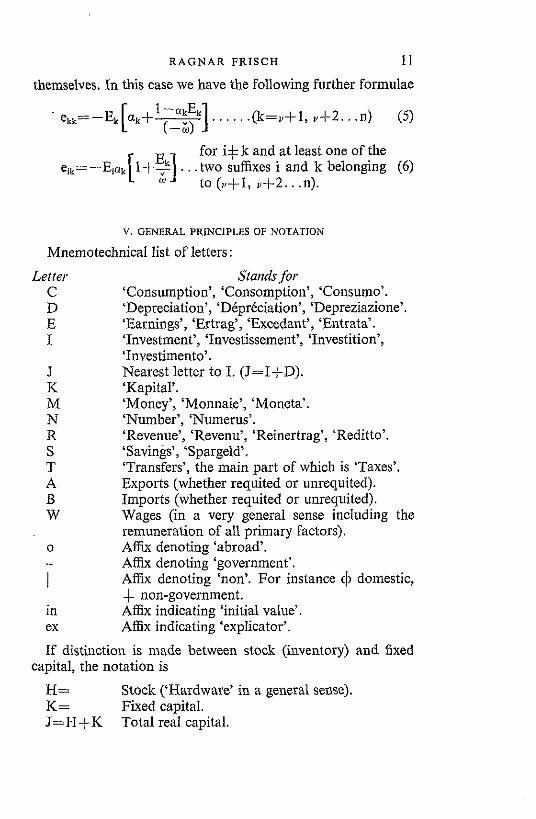
themselves. In this case we have the following further formulae

V. GENERAL PRINCIPLES OF NOTATION

Mnemotechnical list of letters:

Letter Stands for C 'Consumption', 'Consomption', 'Consume'. D 'Depreciation', 'D6prkciation', 'Depreziazione'. E 'Earnings', 'Ertrag', 'Excedant', 'Entrata'. I 'Investment', 'Investissement', 'Investition',

'Investimento'. J Nearest letter to I. (J=I+D). K 'Kapital'. M 'Money', 'Monnaie', 'Moneta'. N 'Number', 'Numerus'. R 'Revenue', 'Revenu', 'Reinertrag', 'Reditto'. S 'Savings', 'Spargeld'. T 'Transfers', the main part of which is 'Taxes'. A Exports (whether requited or unrequited). B Imports (whether requited or unrequited). W Wages (in a very general sense including the

remuneration of all primary factors). o AEx denoting 'abroad'. - Affix denoting 'government'.

I A& denoting 'non'. For instance cb domestic, + non-government. in Affix indicating 'initial value'. ex Affix indicating 'explicator'.

If distinction is made between stock (inventory) and fixed capital, the notation is

H= Stock ('Hardware' in a general sense). K= Fixed capital. J=H+IC Total real capital.


These letters may be used for flows or for flow integrals over time. If usedo for flow integrals, the flows themselves may be denoted H, K, etc. Deviations from initial values are denoted by small letters, for instance C~,*=C~, -C~~. A summation over an affix is denoted by replacing this a f k with a dot. For instance

If a more restricted summation is to be distinguished from a more extensive summation, we may write C:, for the result of the more extensive summation.

Examples of the use of the letters are given in section 2 of a memorandum (in Norwegian) of 6th November 1952 from the University Institute of Economics, Oslo.

VI. THE INPUT-OUTPUT APPROACH

If in the interAow matrix we aggregate all consumption sectors and a number of other rows and columns, we get an input-output table of the usual kind which describes the inter- play between the production sectors. Here one takes consumption as a datum or, at best, as something the changes in which are to be estimated separately through some more or less plausible assumptions. In this way some interesting information can be derived on the production-repercussions. The Central Bureau of Statistics of Norway has recently produced an input- output table for the year 1948. It contained thirty sectors (and a few additional sectors not taken account of in our illput-output computations). In the memorandum just quoted of 6th Novem- ber 1952 the Institute has discussed in great detail a number of specific questions concerned with the computation of the shares of wages, entrepreneurial income, indirect taxes, imports, etc., in the total value of different goods. In connection with this theoretical work a complete inversion of the 30 x 30 matrix was performed. One half of the numerical work in connection with the inversion was done by the Central Bureau of Statistics and the other half by the Institute of Economics. The Institute further comnputed subsidiary tables which made it possible to read off quickly answers to various types of questions. The memorandum is available for those interested.

RAGNAR FRlSCH 13 VI1. THE INTERFLOW MATRIX

When we want to organize our data in a form which is particularly effective from a decision model viewpoint, the pertinent question is always: how can we bring out in the simplest and most striking way those features of the data that are the most important ones for the purpose of estimating the eff'ects ivhiclz ~vould probably be produced by applyi!~g specific economic political measures in an actual sittration.

When a system of national accounts is worked out, one will, of course, always have this in mind to some extent, a t least unconsciously, but the idea is not as explicit and as dominating as it must be when we approach the problem from the viewpoint of a decision model. Other considerations have indeed been given great weight in the construction of a system of national accounts. Examples of these are: to help store the data; to help the statistician in preparing the data for publication; and to help the public in understanding the figures. The degree of complication is also a matter to be considered. Sometimes the accounts themselves are rather complicated. For the purpose of a macro-economic analysis, we need, however, something which is simple enough to make it possible to study the shape of the mathematical solutions in some detail. In a formal way we can, of course, always talce account mathematically of practically everything by introducing a sufEcieut number of letters with a sufficient number of subscripts and superscripts -just as in Walrasian equilibrium theory. But this is not the kind of approach suitable for a decision n~odel. Here we must see to it that it is possible by iilttrition to grasp simultaneously the meaning of all the variables and the particular form of the relations. This demands special care in working out the form of the presentation. Considerations of mnemotechuical and visual ease in grasping the data put specific kinds of requirements on the shape of the main tables, the symbolism, etc.

Therefore, in decision model work we cannot stick to any standardized and sacred accounting system. We must feel free to adopt an approach suitable to the nature of the particular problem at hand.

It seems fairly clear that our requirements cannot be satisfied in any practical way otherwise than by presenting all essential data in some sort of a matrix. But beyond this I think it is impossible to put forward any hard and fast rules concerning


the way in which the data should be organized. Much must bc left to the individual research worker or research group that is struggling with a specific problem with national or local colour.

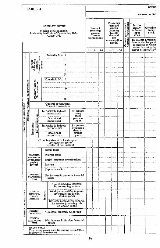
In the work at the University Institute of Economics, Oslo, we have settled on an analytical tool which we call our inte~flo~l 11iatri.u. Its structure is exhibited in Table 11.

The matrix is constructed with the specific purpose of avoiding the complication which is involved in distinguishing between a 'sector' and ail 'account'. From a formal logical point of view there is no need for such a distinction and in a realistic search for what is relevant in a decision model it is not necessary to stick strictly to this distinction.

To see the relativity of the distinction we may for instance consider each 'account' in each 'sector' as a new sector where all transactions are pooled into one account. Take for instance the case where the transactions are entered in an accounting system of n sectors, each with, say, three accounts, a, b, c, represented in a twofold table as that given in Table I. (Each transaction within a sector will be represented by one figure and each transaction between two sectors will be represented by two figures, one in the square of each sector.) Here we can simply renumber all the rows and columns in a continuous fashion from 1 to 3n, and develop rules for handling the 3n-rowed square matrix which emerges. Similarly for any grouping of transactions according to any other - and perhaps even more detailed - principle than that which led to the formation of the concept of an account.

In the huge square matrix which in principle ]nay be constructed in this way, we may start by aggregating rows according to some principle which we find relevant from some viewpoint. For some of the rows we ]nay perhaps perform the aggregation by building on the sector concepts, while for other rows we may decide to aggregate according to some other principle. Also the colunlns may be aggregated in this way. In principle this is a way in which one may visualize the genesis of the intedow matrix. It is in principle a classification of transactions.

The concept of such a matrix is more general than that of an input-output table. The latter is a special sort of interflow matrix.

The interflow lnatrix in Table I may be characterized by the

R A G N A R BRISCH 15

term 'median model' as distinguished from the 'subn~odel' which I described in the Rivue d'Economie Politique for 1951 and the 'supermodel' which we hope to construct in the course of the next few years.

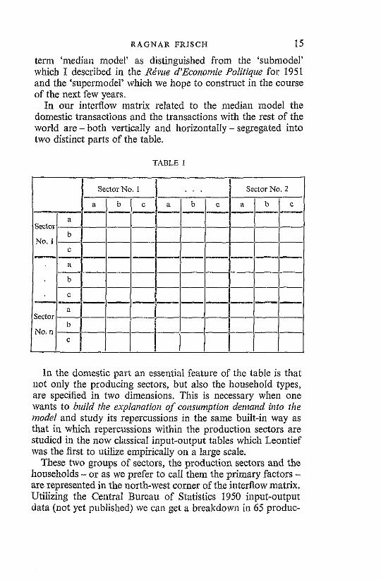
In our interRow matrix related to the median model the domestic transactions and the transactions with the rest of the world are - both vertically and horizontally - segregated into two distinct parts of the table.

TABLE 1

In the donlestic part an essential feature of the table is that not only the producing sectors, but also the household types, are specified in two dimensions. This is necessary when one wants to build the explanation of consumptiotr dentand into the model and study its repercussions in the same built-in way as that in which repercussions within the production sectors are studied in the now classical input-output tables which Leontief was the first to utilize empirically on a large scale.

These two groups of sectors, the production sectors and the households - or as we prefer to call them the primary factors - are represented in the north-west corner of the interflow matrix. Utilizing the Ce~ltral Bureau of Statistics 1950 input-output data (not yet published) we can get a breakdown in 65 produc-

For practical reasons we interpret direct deliveries from households to households as being zero, all goods and services passing through the production sectors. This solution, however, is more or less conventional. Also deliveries from households directly to investment in fixed capital are assumed zero. On the contrary, for government there may be deliveries directly from households.

Next comes the sector general government. It is taken in the


tion sectors, of which one is a sector for domestic trade in non-competitive import goods. On the basis of the Institute's own work we believe we can get rough estimates for 45 household types classified as shown in Table III.

TABLE 111

"This group also includes all households consj,ting of one adult a.tth one or murc children, regdrdlcss of t l w n:iturr of th- income (14,300 household, o ~ r of a total of 980,000).

Non-profit institutions serving households . . . . 45

Two Adults

with Onc w more Children

3 7

I I

15

19 23

27 31 35

39

43

Types of 1-Iouschold (Primary Factors)

One Adult

without Children

1 5

9 13

17 21

25 29

33

37

41

Three or more

Adults with One or more Children

4 8

12 16

20 24

28 32 36

40

44

Urban districts

Rural districts

Two or more Adults without Children

2 6

10 14

18 22

26 30 34

38

42

Workers (wage earners) Salaried persons . . Small employers and workers on own account

Larger employers . Workers (wage earners) Salaried persons . . Small employers and workers on own account Smaller farmers . . Fishermen . . . Larger farmers and for- est owners . .

Persons living on pension (rural and urban districts together)' .


accepted sense of the 'Standardized System of National Accounts'.l

After general governnlent in our interflow matrix comes a section pertaining to . investment (all previously considered transactions being current ones). We have found it convenient to make a basic distinction between changes in inventories (stocks) and changes in fixed capital, and, within inventories, to distinguish between those which enterprises maintain of what are for them input goods, and those which they maintain of what are for them output goods. In both categories we distinguish between an intrinsically induced part, that is a part which is theoretically to be connected with other elements of the interflow matrix in some way, and another part which (intentionally or unintentionally) varies in a way which it is not considered the purpose of the median model, built on the interflow table, to explain. In other words these parts are taken as spontaneously determined elements (elements determined from the outside).

All the transactions considered so far have been of what might be called the physical sort. Next comes a part of the table containing transfers.

To describe without ambiguity what this distinction means, a few words of an axion~atic sort are needed.

I l'obl:sIted by the 0.E.t .C. . I?IIIS, 1952. We haw trled lo folluw the main ide:ts ofthis report :I, FJr ns consistent with the pupuse of the de;lsion model. For

taxes are iiandleddiferehtly. If the indirect taxes (minus subsidies) are subtracted from the profits of the cnrirprisw (which m.6). bc n nnturill thinglo do), why arc not these raxcs themsel~es en~crcd as n s c p ~ r . ~ t c item in the national income? In nrinciolc the diffcrcnce bctucen lhc l a o dtducrions in oustion onlv rcsidcs in thc modebf Davment of a Droductive function. If we keeo iuch dcduciions out of the n~iional ;ncomc conccbt, ahy csn we nor just as well also keep ,\ages out of it? This M L ) U I ~ lend to thz cunclusion rh:tr only the profils of the enterprises are a true' and 'real'contr~butiun lo national incums, 3 conclusion 1h3t may xppral to

some. As I see it, the standardized method leadins to the concept of national income of

factor cost - snd to the cmph:~sis on i t - is n?nhingmore th:tn ;t hcrit3ge from the rintz when all soru of govcrnrn:nr ~n~t~ ; t t i \ e in cso.~omlc mnttcrs $re,< banned as a nuisance iud \\.hen co~?,cauenrlv !zu\.crnmmr was nor cunsidercd a 'iacror oi ~roduction' at all. and uanicuiarlj. i o t that Dart of its activity which was made

values reckoned at inarket price.


To begin with we take for granted the concept of a flow and also the distinction between aphysical object (a brick, a kilo of butter, etc.) and afina~tcial object (a bank note, a claim, etc.). How the distinction is to be made in practice is a matter of convention, but in most cases the difference will be clear enough. Next we introduce the distinction between a requited flow (one to be paid for) and an unrequited flow (one not to be paid for). Requited flows always occur in pairs, one of them going one way and an exactly equal flow going in the opposite direction. (On the delivery of a physical object either a claim or cash moves in the opposite direction.) In other words requited flows are bilateral. The unrequited flows are unilateral.

Combining the two classifications, we find that an unrequited flow may be either physical or financial. A pair of corresponding requited flows may fall in one of three categories: either both flows are physical (barter), or one is physical, the other financial (most transactions in which a producing sector or a household takes part), or both are financial (banking operations and operations on the stock or bond market). Thus we have five types of transactions, namely:

UirrequitedJloivs (1) A physical object; (2) A financial object.

Requitedfloti~s (3) Both objects physical; (4) Both objects financial; (5) One of the objects physical, the other financial.

In a complete analysis an attempt should be made to keep these five types of transactions entirely separate. At the present stage we must, however, look for a simplification.

One way to simplify which has sometimes been attempted is to consider all flows as being of the requited type, with one of the flows in the pair a physical object and the other a financial object. This maltes it necessary in many cases to impute (imagine) counterflows either physical or financial. If this system were to be carried through logically to the bitter end, it would become very cumbersome and one would run into many extremely artificial constructions. In our work we have completely abandoned this approach. We do not want to refrain

R A G N A R FRISCH 2 1

entirely from the consideration of imputed flows, but only to restrict their use as much as possible. This means that we are still left with the above five categories.

Our attempt at simpUcation consists in the following. First we refrain at the present stage from an explicit study of the requited flows where one financial object moves against another financial object. In other words we detach the study of the money and credit market from the present analysis, main- taining the contact only at one strategic poirzt, namely through the balancing item: net increase in financial assets (considered separately for domestic and foreign assets). When a special study of the money and credit market is later completed with due consideration of the various types of financial objects, their market conditions, demand and supply peculiarities, etc., this whole study can be linked to the present one through the balancing item. To be sure, this is not the ideal solution, but at the moment it is the best we can do.

In the second place, if an unrequited flow of a physical object (a gift in kind) should occur, we look upon it as an unrequited flow of a financial object (a gift of a financial object) followed by a pair of requited flows consisting of one physical object moving against one financial object.

We are then left with the following three types: an unrequited flow of a hancial object, a requited flow where both objects are physical, and a requited flow where one object is physical and the other financial. The first we call a tuansfer, the second two categories we unite under the common name of a physical tr.ansactio~z. Whatever financial elements may be involved in the types of flow included in the physical transactions cannot cause much trouble because we only consider the financial effects in so far as they are registered in the net change of financial assets. It is the physical parts of the transactions which ulill form the main object of ihc study. Because of our simplifying construction it is easy to consider each flow separately without necessarily considering simultaneously the flow and the counter- Aow.

In Table I the dichotomy between the part describing the physical transactions and the part describing the transfers is applied both in the domestic part and in the foreign part of the table.

Within the domestic transfer part we have used the categories C


direct taxes, inclirect taxes, social insurance transfers and capital transfers. They correspond very much to the categories of the 'Standardized System'.

Under imports a distinction is made between non-competitive, weakly competitive and strongly competitive imports. The competitive imports may be entered either as negative numbers in a column or as positive numbers in a row. We have preferred the latter alternative.

The receiving side of the table is very much like the delivering side except for the fact that we have found it necessary on the receiving side to distinguish between government and non- government investment in fixed capital.

For the production sectors, the primary factors (the households) and general government the table is completely balanced in the sense that the grand total in any row is equal to the grand total in the corresponding column. The sum in the row represents total purchasing power acquired by the sector and the sum in the column represents total purchasing power used by it (including net increase in financial investment).

A few examples may illustrate the meaning of rows and columns. Xk, is the value of goods which have been used in the accounting period by the sector ir, and is of the kind produced by sector X. If it is to be possible to relate X i F to any sort of technical coefficients, it must be defined as the quantity used by ir,. Similarly for the quantity Chy representing goods of the X-type consumed by the consumer demand group y. The goods entering into Xi, may have been produced by A in the accounting period, or taken from the stock of X-goods or imported (as competitive imports) in the same accounting period. But it cannot be considered as being talten from any special stock of import goods because competitive imports are Iooked upon as going to the national sector and resting there as a stock if it is not used immediately.

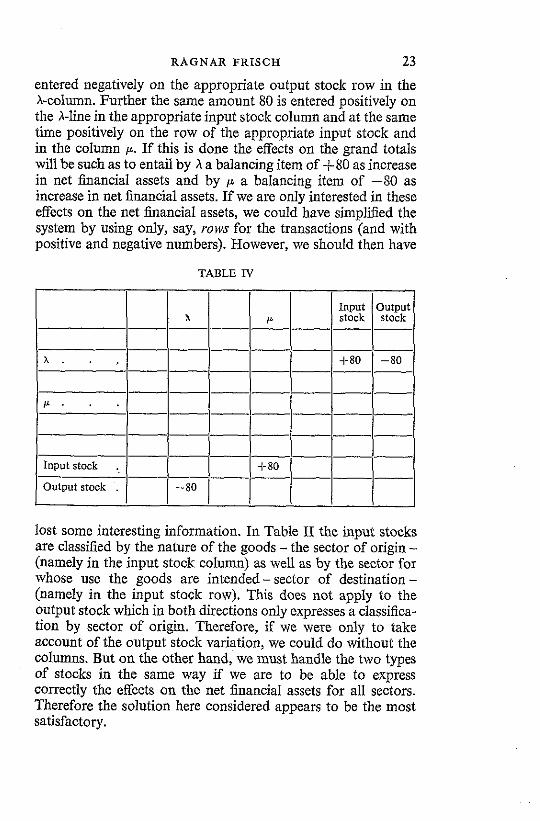
As an example of the handling of goods passing from an output stock to an input stoclc consider the following. Suppose that a value of 80 is taken from the output stock of sector X - goods that may have been produced by A or imported as competitive imports - and placed in the input stock of sector g. The entries representing this transaction are made as indicated in Table IV. In the first place 80 is entered negatively on the A-line in the appropriate output stock column and at the same time

RAGNAR FRISCH 23

entered negatively on the appropriate output stock row in the A-column. Further the same amount 80 is entered positively on the A-line in the appropriate input stock column and at the same time positively on the row of the appropriate input stock and in the column p. If this is done the effects on the grand totals will be such as to entail by X a balancing item of +80 as increase in net financial assets and by p a balancing item of -80 as increase in net financial assets. If we are only interested in these effects on the net financial assets, we conld have simplified the system by using only, say, rows for the transactions (and with positive and negative numbers). However, we should then have

TABLE N

lost some interesting information. In Table 11 the input stocks are classzed by the nature of the goods - the sector of origin - (namely in the input stock column) as well as by the sector for whose use the goods are intended-sector of destination - (namely in the input stock row). This does not apply to the output stock which in both directions only expresses a classification by sector of origin. Therefore, if we were only to take account of the output stock variation, we conld do without the columns. But on the other hand, we must handle the two types of stocks in the same way if we are to be able to express correctly the effects on the net financial assets for all sectors. Therefore the solution here considered appears to be the most satisfactory.

A . . ,

P . . .

Input stock . Output stock .

x

- 80

P ------- ------- ------- ------- ------- ------- ----ppp + 80 -------

Input stock

1-80

Output stock

-80


It should be noticed that for ally of the stocks it is not the difference between the row-sum and the column-sum that expresses the net effect, but the net effect is akeady given in either a row or a column.

VIII. THE RELATIONS IN THE INTERFLOW MATRIX: INYERSION PROBLEMS

The approach to the decision model problem through Table I1 is certainly not as complete as we would like. For instance, in this table only certain rather simple types of price effects can be studied. We do not get the full picture of con- sumers' adaptation under the influence of the want-structures, nor do we get a clear expression for the pressure coefficients. In these respects the submodel was much more satisfactory. But in other respects it was all too simple and its numerical structure was based almost entirely on guesswork. The median model on which we are now working contains much more empirical material.

To utilize this material, we need to assume certain types of relations. In short we may say that we do not assume propor- tionality, but do assume linearity. More precisely the assumptions can be formulated as follows. The starting point is an interflow matrix of absolute figures pertaining to a given year, 1950. In addition to this another matrix will be used, namely a matrix of coeficienfs that express what proportiorzs the change of the variables in question can be assumed to bear to the corresponding change in some explicators. Each such explicator is defined as a linear form in the other items of the table. In principle it may be a general linear form of all the items, but in practice most of these linear forms will contain only certain groups of the items, for instance the items in certain columns or the items in certain rows.

When an estimate is to be made of foreseeable effects of changes, certain of the items of the model are taken as changing data, and the rest computed through the equations. These data that change are not localized to some specific row or some specific column, but may be distributed in a more complex way in the table. Suck a complex distribution is inevitabIe in many of the speciEc questions we want to answer by means of the table. I shall not go it1 detail through the method by which the equations may be worked out, but only suggest the simple example indicated in Table IV.

RAGNAR FRISCH 25

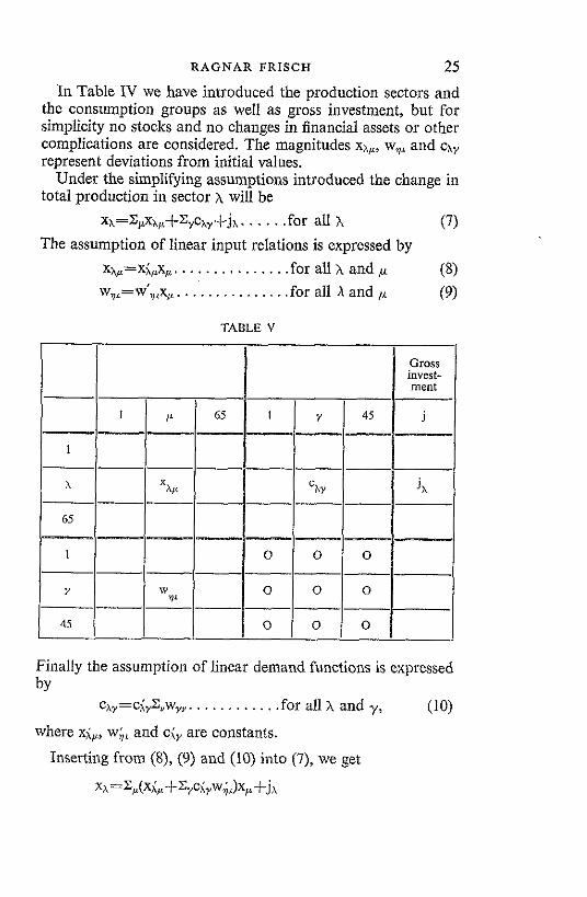
In Table IV we have introduced the production sectors and the consumption groups as well as gross investment, but for simplicity no stocks and no changes in financial assets or other complications are considered. The magnitudes xA,, w,,, and cAy represent deviations from initial values.

Under the simplifying assumptions introduced the chauge in total production in sector x will be

x ~ = Z , , x . ~ h ~ + Z ~ c ~ ~ + j ~ . . . . . .for all x (7) The assumption of linear input relations is expressed by

X ~ ~ = X ~ , ~ X , . . . . . . . . . . . . . . .for all x and (8) w,,=w',,x,. . . . . . . . . . . . . . .for all h and (9)

TABLE V

Finally the assuniption of linear demand functions is c~pressed by

c~~=ci,Z,w~, . . . . . . . . . . . .for all X and y, (10) where xi,, w;, and ci, are constants.

Inserting from (S), (9) and (10) into (7), we get

x~=X,(x i~f ~ y ~ i y ~ ; L ) ~ p + j h


which may also be written

~ f i [ e ~ , u - ( x ; c p + ~ ~ c ~ Y ~ ~ L ) ] ~ P = j ~ . . . . . .for all X (1 1) where ek, are the unit numbers, i.e. 1 when x = ~ and 0 when xso. This is a system of linear equations in the x,, of the familiar input-output form, only with coefficients that are to be computed by a matrix multiplication. The inversion problen- which numerically is the only thing that counts - will be the same as in the usual input-output analysis.

When the total production levels are determined through (1 1) the individual items are computed by (8), (9) and (10).

In Oslo we are fortunate in having an electronic computor which will be put into operation in a few months. For the time being its high-speed memory is very limited, so one has to resort to repunching for problems with as many variables as we have. Nevertheless the saving in time over work done on desk com- putors is considerable. A large-scale electronic compntor will be available in about a year.

We shall try to introduce a dynanuc viewpoint by means of a lag matrix, that is a matrix expressing the average time lag one can assume between the deliveries from each sector and the emergence of the goods from each sector that uses the first- mentioned goods as input elements. I believe that this is a more practical and promising way to attack the dynamic aspect than through differential equations. The technique of lag matrices was the subject of lectures I delivered in Oslo University last year. They are being published in mimeographed form.

The estimation of the coefficients needed and the setting up of sigiificance levels for the conclusions is a chapter all by itself. I shall not go into that subject in this connection.

from national accounts to macro-economic decision models

Documents