From normal to anomalous diffusion in comb-like structures in three dimensionsAlexander M. Berezhkovskii, Leonardo Dagdug, and Sergey M. Bezrukov

Citation: The Journal of Chemical Physics 141, 054907 (2014); doi: 10.1063/1.4891566 View online: http://dx.doi.org/10.1063/1.4891566 View Table of Contents: http://scitation.aip.org/content/aip/journal/jcp/141/5?ver=pdfcov Published by the AIP Publishing Articles you may be interested in Improved volumetric measurement of brain structure with a distortion correction procedure using an ADNIphantom Med. Phys. 40, 062303 (2013); 10.1118/1.4801913 Diffusion tensor imaging using a high-temperature superconducting resonator in a 3 T magnetic resonanceimaging for a spontaneous rat brain tumor Appl. Phys. Lett. 102, 063701 (2013); 10.1063/1.4790115 A method for estimation of stimulated brain sites based on columnar structure of cerebral cortex in transcranialmagnetic stimulation J. Appl. Phys. 105, 07B303 (2009); 10.1063/1.3068631 Estimation of cell membrane permeability of the rat brain using diffusion magnetic resonance imaging J. Appl. Phys. 103, 07A311 (2008); 10.1063/1.2830534 Conductivity tensor imaging of the brain using diffusion-weighted magnetic resonance imaging J. Appl. Phys. 93, 6730 (2003); 10.1063/1.1544446

This article is copyrighted as indicated in the article. Reuse of AIP content is subject to the terms at: http://scitation.aip.org/termsconditions. Downloaded to IP:

130.63.180.147 On: Wed, 13 Aug 2014 11:28:39

THE JOURNAL OF CHEMICAL PHYSICS 141, 054907 (2014)

From normal to anomalous diffusion in comb-like structuresin three dimensions

Alexander M. Berezhkovskii,1,2 Leonardo Dagdug,1,2,a) and Sergey M. Bezrukov1

1Program in Physical Biology, Eunice Kennedy Shriver National Institute of Child Health and HumanDevelopment, National Institutes of Health, Bethesda, Maryland 20892, USA2Mathematical and Statistical Computing Laboratory, Division for Computational Bioscience,Center for Information Technology, National Institutes of Health, Bethesda, Maryland 20892, USA

(Received 29 May 2014; accepted 16 July 2014; published online 7 August 2014)

Diffusion in a comb-like structure, formed by a main cylindrical tube with identical periodic deadends of cylindrical shape, occurs slower than that in the same system without dead ends. The reasonis that the particle, entering a dead end, interrupts its propagation along the tube axis. The slowdownbecomes stronger and stronger as the dead end length increases, since the particle spends more andmore time in the dead ends. In the limiting case of infinitely long dead ends, diffusion becomesanomalous with the exponent equal to 1/2. We develop a formalism which allows us to study themean square displacement of the particle along the tube axis in such systems. The formalism isapplicable for an arbitrary dead end length, including the case of anomalous diffusion in a tube withinfinitely long dead ends. In particular, we demonstrate how intermediate anomalous diffusion ariseswhen the dead ends are long enough. [http://dx.doi.org/10.1063/1.4891566]

I. INTRODUCTION

The model of a particle diffusing in a tube with dead endsis widely used in studies of linear porous media.1–3 Examplesof transport in such systems include transport in dendrites,4

extra-cellular diffusion in brain tissue,5 diffusion of water andother substances in muscles,6 etc. An analytical theory of dif-fusion in tubes with periodic dead ends formed by identicalcavities connected to the main tube by narrow necks has beendeveloped in Ref. 3(a)). The focus of the present study is ona special case of such a tube, where the dead ends are peri-odic thin cylinders. This is the so-called comb-like structureschematically shown in Fig. 1. The mean square displacement〈x2(t)〉 of a particle diffusing in such a structure has qualita-tively different long-time behavior depending on whether thedead end length is finite or infinite. When the length is finite〈x2(t)〉|t→∞ ∝ t, while when the length is infinite 〈x2(t)〉|t→∞∝ t1/2. Thus, at a finite dead end length we deal with normaleffective diffusion, whereas when this length is infinite, thediffusion is anomalous.7–10

When the dead ends are long enough, the particle is“unaware” of their finiteness at intermediate times. As a re-sult, anomalous-like diffusion naturally arises during the tran-sient behavior to the effective normal diffusion at long times.Such transient behavior can be misinterpreted as anomalousdiffusion.11 Intermediate anomalous diffusion in cells andother complex environments has been discussed recently.7–11

Diffusion and random walk in comb-like structures havebeen studied by many authors (see, for example, the booksby Weiss12 and Redner13 and references therein). A distinc-tive feature of the present study is that we develop a formal-ism which allows us to derive an expression for the Laplace

a)Permanent address: Physics Department, Universidad AutonomaMetropolitana-Iztapalapa, 09340 Mexico City, Mexico.

transform of the mean square displacement 〈x2(t)〉, which isapplicable for an arbitrary comb tooth length. This is done inSec. II. Inverting this transform numerically, one can obtainthe mean square displacement over the entire range of time.In Sec. III, we use this transform to analyze the behavior of〈x2(t)〉 at short and long times. In addition, we demonstrateintermediate anomalous subdiffusion, 〈x2(t)〉 ∝ t1/2, duringthe transition to the effective normal diffusion at long times.The obtained results are summarized and some concluding re-marks are made in Sec. IV.

II. GENERAL THEORY

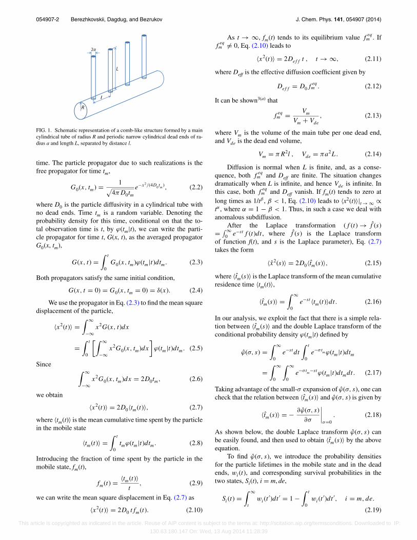
Consider a point particle diffusing in a comb-like struc-ture schematically shown in Fig. 1. The structure is formed bya main cylindrical tube of radius R and periodic thin cylindri-cal dead ends of radius a and length L, separated by distance l.The cylinders are thin in the sense that their radius a is muchsmaller than both the period l and the main tube radius R,a � l, R. The dead end length L can be arbitrary, L ≥ 0. Thecase of L = 0 corresponds to a purely cylindrical tube with nodead ends. The particle propagates along the tube axis onlywhen it is in the main tube. Entering a dead end, the particleinterrupts its propagation. Later it returns, and the propaga-tion continues. Particle transitions between the main tube andthe dead ends can be described as transitions between mobile(m) and immobile (de) states by the kinetic scheme

m →← de. (2.1)

We assume that the particle starts in the main tube andchoose its starting position along the tube axis as the ori-gin. Consider those realizations of the particle trajectory, forwhich the cumulative time spent by the particle in the mobilestate is equal to tm, tm ≤ t, where t is the total observation

0021-9606/2014/141(5)/054907/7/$30.00 141, 054907-1

This article is copyrighted as indicated in the article. Reuse of AIP content is subject to the terms at: http://scitation.aip.org/termsconditions. Downloaded to IP:

130.63.180.147 On: Wed, 13 Aug 2014 11:28:39

054907-2 Berezhkovskii, Dagdug, and Bezrukov J. Chem. Phys. 141, 054907 (2014)

FIG. 1. Schematic representation of a comb-like structure formed by a maincylindrical tube of radius R and periodic narrow cylindrical dead ends of ra-dius a and length L, separated by distance l.

time. The particle propagator due to such realizations is thefree propagator for time tm,

G0(x, tm) = 1√4πD0tm

e−x2/(4D0tm), (2.2)

where D0 is the particle diffusivity in a cylindrical tube withno dead ends. Time tm is a random variable. Denoting theprobability density for this time, conditional on that the to-tal observation time is t, by ϕ(tm|t), we can write the parti-cle propagator for time t, G(x, t), as the averaged propagatorG0(x, tm),

G(x, t) =∫ t

0G0(x, tm)ϕ(tm|t)dtm. (2.3)

Both propagators satisfy the same initial condition,

G(x, t = 0) = G0(x, tm = 0) = δ(x). (2.4)

We use the propagator in Eq. (2.3) to find the mean squaredisplacement of the particle,

〈x2(t)〉 =∫ ∞

−∞x2G(x, t)dx

=∫ t

0

[∫ ∞

−∞x2G0(x, tm)dx

]ϕ(tm|t)dtm. (2.5)

Since ∫ ∞

−∞x2G0(x, tm)dx = 2D0tm, (2.6)

we obtain

〈x2(t)〉 = 2D0〈tm(t)〉, (2.7)

where 〈tm(t)〉 is the mean cumulative time spent by the particlein the mobile state

〈tm(t)〉 =∫ t

0tmϕ(tm|t)dtm. (2.8)

Introducing the fraction of time spent by the particle in themobile state, fm(t),

fm(t) = 〈tm(t)〉t

, (2.9)

we can write the mean square displacement in Eq. (2.7) as

〈x2(t)〉 = 2D0 tfm(t). (2.10)

As t → ∞, fm(t) tends to its equilibrium value feqm . If

feqm �= 0, Eq. (2.10) leads to

〈x2(t)〉 = 2Deff t , t → ∞, (2.11)

where Deff is the effective diffusion coefficient given by

Deff = D0feqm . (2.12)

It can be shown3(a) that

feqm = Vm

Vm + Vde

, (2.13)

where Vm is the volume of the main tube per one dead end,and Vde is the dead end volume,

Vm = πR2l , Vde = πa2L. (2.14)

Diffusion is normal when L is finite, and, as a conse-quence, both f

eqm and Deff are finite. The situation changes

dramatically when L is infinite, and hence Vde is infinite. Inthis case, both f

eqm and Deff vanish. If fm(t) tends to zero at

long times as 1/tβ , β < 1, Eq. (2.10) leads to 〈x2(t)〉|t → ∞ ∝tα , where α = 1 − β < 1. Thus, in such a case we deal withanomalous subdiffusion.

After the Laplace transformation (f (t) → f (s)= ∫ ∞

0 e−stf (t)dt , where f (s) is the Laplace transformof function f(t), and s is the Laplace parameter), Eq. (2.7)takes the form

〈x2(s)〉 = 2D0〈tm(s)〉, (2.15)

where 〈tm(s)〉 is the Laplace transform of the mean cumulativeresidence time 〈tm(t)〉,

〈tm(s)〉 =∫ ∞

0e−st 〈tm(t)〉dt. (2.16)

In our analysis, we exploit the fact that there is a simple rela-tion between 〈tm(s)〉 and the double Laplace transform of theconditional probability density ϕ(tm|t) defined by

ϕ(σ, s) =∫ ∞

0e−st dt

∫ t

0e−σ t

mϕ(tm|t)dtm

=∫ ∞

0

∫ ∞

0e−σ t

m−stϕ(tm|t)dtmdt. (2.17)

Taking advantage of the small-σ expansion of ϕ(σ, s), one cancheck that the relation between 〈tm(s)〉 and ϕ(σ, s) is given by

〈tm(s)〉 = − ∂ϕ(σ, s)

∂σ

∣∣∣∣σ=0

. (2.18)

As shown below, the double Laplace transform ϕ(σ, s) canbe easily found, and then used to obtain 〈tm(s)〉 by the aboveequation.

To find ϕ(σ, s), we introduce the probability densitiesfor the particle lifetimes in the mobile state and in the deadends, wi(t), and corresponding survival probabilities in thetwo states, Si(t), i = m, de,

Si(t) =∫ ∞

t

wi(t′)dt ′ = 1 −

∫ t

0wi(t

′)dt ′, i = m, de.

(2.19)

This article is copyrighted as indicated in the article. Reuse of AIP content is subject to the terms at: http://scitation.aip.org/termsconditions. Downloaded to IP:

130.63.180.147 On: Wed, 13 Aug 2014 11:28:39

054907-3 Berezhkovskii, Dagdug, and Bezrukov J. Chem. Phys. 141, 054907 (2014)

We use these survival probabilities and probability densities towrite a linear integral equation for the conditional probabilitydensity ϕ(tm|t),ϕ(tm|t) = Sm(t)δ(tm − t) + wm(tm)Sde(t − tm)

+∫ t

0wm(t ′)dt ′

∫ t−t ′

0wde(t ′′)ϕ(tm−t ′|t−t ′−t ′′)dt ′′.

(2.20)

The first term on the right-hand side of this equation repre-sents those realizations of the particle trajectory, which do notenter a dead end and spend all the time in the main tube. Forsuch trajectories we have tm = t. The second term representstrajectories which spend time tm in the main tube, then enter adead end, and never return to the main tube. The third term isdue to realizations that escape from the main tube and comeback at least once.

After the double Laplace transformation, Eq. (2.20) takesthe form

ϕ(σ, s) = Sm(s + σ ) + wm(s + σ )Sde(s)

+ wm(s + σ )wde(s)ϕ(σ, s). (2.21)

Solving this equation we obtain

ϕ(σ, s) = Sm(s + σ ) + wm(s + σ )Sde(s)

1 − wm(s + σ )wde(s). (2.22)

Finally, we take advantage of the relation between Si(s) andwi(s), which follow from Eq. (2.19),

Si(s) = 1

s(1 − wi(s)), i = m, de. (2.23)

This allows us to write Eq. (2.22) as

ϕ(σ, s)= s(1−wm(s+σ )wde(s))+σwm(s+σ )(1−wde(s))

s(s+σ )(1−wm(s+σ )wde(s)).

(2.24)Substituting this expression for ϕ(σ, s) into Eq. (2.18), we ar-rive at

〈tm(s)〉 = 1 − wm(s)

s2(1 − wm(s)wde(s)). (2.25)

To finish the derivation, it remains to specify the proba-bility densities of the particle lifetimes in the two states, wm(t)and wde(t). We begin with the former. For a particle diffusingin the main tube, entry into a dead end may be consideredas trapping by the dead end entrance. Then, for the particlein the main tube, the boundary conditions on the tube wallare non-uniform: absorbing on the disks of radius a formingthe dead end entrances and reflecting on the rest of the tubewall. One can approximately describe trapping by such non-uniform boundary using boundary homogenization, which isthe replacement of the initial non-uniform boundary by aneffective uniformly absorbing boundary with correctly cho-sen effective trapping rate. (One can learn more about bound-ary homogenization in papers cited in Ref. 14, and referencestherein.) Since the disk surface fraction is small, a2/(Rl) � 1,the effective trapping rate of the boundary, κ , is given by14

κ = 4D0a

2πRl= 2D0a

πRl. (2.26)

This is in fact a linearized version of the Berg-Purcell-Shoup-Szabo formula15, 16 for the effective trapping rate by a patchysurface.

The trapping rate in Eq. (2.26) is very low in the sensethat the radial relaxation time, τ rel, is much shorter than thetrapping time, τ tr, found assuming uniform distribution of theparticle over the main tube cross section. To show this, wenote that τ rel ∝ R2/D0, while τ−1

tr = 2κ/R ∝ D0a/(R2l). So,the ratio of the two times is

τrel

τtr

∝ a

l� 1. (2.27)

Since τ rel � τ tr, the particle survival probability in the mobilestate decays as a single exponential, Sm(t) = e−k

mt , where the

rate constant km is given by

km = 1

τtr

= 2κ

R= 4D0a

Vm

. (2.28)

Respectively, the probability density for the particle lifetimein the main cylindrical part of the tube is

wm(t) = −dSm(t)

dt= kme−k

mt . (2.29)

The Laplace transform of wm(t) has the form

wm(s) = km

s + km

. (2.30)

Substituting this transform into Eq. (2.25), we arrive at

〈tm(s)〉 = 1

s[s + km(1 − wde(s))]. (2.31)

Finally, the Laplace transform of the probability densityof the particle lifetime in the dead end can be found using theresults obtained in Ref. 3(a)), where the escape from a deadend of a more general shape is considered. For a cylindricaldead end of length L and radius a, wde(s) is given by

wde(s) = κde

κde + √sDde tanh(L

√s/Dde)

, (2.32)

where Dde is the particle diffusivity in the dead end, whichmay differ from the diffusivity D0 in the main tube, and pa-rameter κde is17

κde = 4D0

πa. (2.33)

The case of L = 0 corresponds to the tube without dead ends.In this case, according to Eq. (2.32), we have wde(s) = 1.Substituting this into Eq. (2.31), we obtain 〈tm(s)〉 = 1/s2. In-verting this Laplace transform we find that 〈tm(t)〉 = t, as itmust be in the absence of dead ends, since the particle spendsall time in the mobile state. For infinitely long dead ends,Eq. (2.32) simplifies and takes the form

wde(s)|L=∞ = κde

κde + √sDde

. (2.34)

The expressions in Eqs. (2.15), (2.31), and (2.32) allowus to find the Laplace transform of the mean square dis-placement, 〈x2(s)〉, at arbitrary length L of the dead ends. InSec. III, we use these expressions to study the long-time be-havior of 〈x2(t)〉 as a function of L.

This article is copyrighted as indicated in the article. Reuse of AIP content is subject to the terms at: http://scitation.aip.org/termsconditions. Downloaded to IP:

130.63.180.147 On: Wed, 13 Aug 2014 11:28:39

054907-4 Berezhkovskii, Dagdug, and Bezrukov J. Chem. Phys. 141, 054907 (2014)

III. APPLICATION OF THE THEORY

Having in hand the Laplace transform 〈x2(s)〉, one canobtain the mean square displacement over the entire range oftime by inverting the transform numerically. In addition, onecan use asymptotic behavior of 〈x2(s)〉 at large and small val-ues of the Laplace parameter to find the short- and long-timebehavior of 〈x2(t)〉, respectively. As s → ∞, wde(s) → 0, andEq. (2.31) reduces to

〈tm(s)〉 ≈ 1

s2− km

s3, s → ∞. (3.1)

Inverting this Laplace transform we find the short-time behav-ior of 〈tm(t)〉,

〈tm(t)〉 ≈ t − km

t2

2, t → 0. (3.2)

Then the fraction of time spent by the particle in the maintube, Eq. (2.9), and the mean square displacement, Eq. (2.10),at short times, respectively, are

fm(t) ≈ 1 − 1

2kmt , t → 0, (3.3)

〈x2(t)〉 ≈ 2D0t − D0kmt2 , t → 0. (3.4)

The relations in Eqs. (3.2)–(3.4) are universal in the sensethat they are independent of the dead end length L, assumingthat L �= 0. This is quite natural since the particle, startingin the main tube, is unaware of the dead end length at shorttimes. However, the long-time behaviors of 〈tm(t)〉, fm(t), and〈x2(t)〉 are not universal. Moreover, they are qualitatively dif-ferent depending on whether the dead ends are of finite or in-finite length. Therefore, below we analyze the two cases sep-arately starting with the latter one.

A. Infinitely long dead ends

When the dead ends are infinitely long, we find theLaplace transform of 〈tm(t)〉 by substituting into Eq. (2.31)the expression for wde(s)|L=∞ given in Eq. (2.34). This leadsto

〈tm(s)〉 = κde + √Ddes

s(km

√Ddes + κdes + √

Dde s3/2) . (3.5)

The leading term of the small-s asymptotic behavior of 〈tm(s)〉is

〈tm(s)〉 ≈ κde

km

√Dde s3/2

, s → 0. (3.6)

Inverting this Laplace transform we find the long-time behav-ior of 〈tm(t)〉,

〈tm(t)〉 ≈ 2κde√πDde km

√t , t → ∞. (3.7)

The long-time behavior of fm(t) and 〈x2(t)〉 can be re-spectively found by substituting 〈tm(t)〉 given in Eq. (3.7) intoEqs. (2.9) and (2.10). The results are

fm(t) ≈ 2κde

km

√πDdet

, t → ∞ (3.8)

and

〈x2(t)〉 ≈ 2D0κde√πDde km

√t , t → ∞. (3.9)

Using Eqs. (2.28) and (2.33), we can write the long-timebehaviors of fm(t) and 〈x2(t)〉 given in Eqs. (3.8) and (3.9)in terms of the geometric parameters of the system, volumeVm = πR2l and the area of the dead end entrance, Ade = πa2,

fm(t) ≈ 2Vm

Ade

√πDdet

, t → ∞ (3.10)

and

〈x2(t)〉 ≈ 2D0Vm

Ade

√t

πDde

, t → ∞. (3.11)

The expressions in Eqs. (3.9) and (3.11) show that incomb-like structures with infinitely long dead ends diffusionis anomalous with the exponent α = 1/2. This is a conse-quence of the fact that the fraction of time spent by the parti-cle in the main tube (mobile state) tends to zero at long timesas 1/t1/2, Eqs. (3.8) and (3.10). Thus, in comb-like structureswith infinitely long teeth the exponents α and β are equal toeach other, α = β = 1/2. The range of applicability of theasymptotic results discussed above is given by

t � κ2de

k2mDde

= V 2m

A2deDde

. (3.12)

This inequality follows from the requirement that the small-s expansion of the Laplace transform of 〈tm(t)〉, Eq. (3.5), isdetermined by its leading term, Eq. (3.6).

Finally, we define function α(t), which can be interpretedas a time-dependent analog of the exponent α,

α(t) = d ln〈x2(t)〉d ln t

= 1 + d ln fm(t)

d ln t, (3.13)

where the second equality follows from the first one andEq. (2.10). According to Eq. (3.3), and Eqs. (3.8) and (3.10)liming values of this function are

α(t) ≈{

1, t → 0

1/2, t → ∞. (3.14)

Solid lines in Fig. 2 show the time dependences fm(t),〈x2(t)〉, and α(t) obtained by numerically inverting the Laplacetransforms 〈tm(s)〉, Eq. (3.5), and s〈tm(s)〉. The curves weredrawn assuming that R = l = 1, a = 0.1, and D0 = Dde =1. In the rest of this section, we discuss how the dependencesfm(t), 〈x2(t)〉, and α(t) are modified when the dead ends are offinite length, and how they are affected by the difference inthe diffusivities D0 and Dde.

B. Dead ends of finite length

When the dead end length is finite, the Laplace transformof the probability density of the particle lifetime in the deadend is given by Eq. (2.32). Substituting this transform into

This article is copyrighted as indicated in the article. Reuse of AIP content is subject to the terms at: http://scitation.aip.org/termsconditions. Downloaded to IP:

130.63.180.147 On: Wed, 13 Aug 2014 11:28:39

054907-5 Berezhkovskii, Dagdug, and Bezrukov J. Chem. Phys. 141, 054907 (2014)

1×100 1×102 1×104 1×106 1×108

time

0

0.1

0.2

0.3

0.4

0.5

0.6

0.7

0.8

0.9

1f m

L = 10

L = 102

L = 103

L = ∞

0 2×104 4×104 6×104 8×104 1×105

time

0

5×104

1×105

2×105

2×105

<x2

> L = 10

L = 102

L = ∞

L = 0

(a) (b)

(c)

FIG. 2. The time dependences of the fraction of time spent by the particle in the main tube, fm(t), panel (a), the mean square displacement, 〈x2(t)〉, panel (b),and function α(t), panel (c), defined in Eqs. (2.7), (2.9), and (3.13), respectively. Solid curves show the dependences for the tube with infinitely long dead ends,L = ∞, while the dashed lines show these dependences for tubes with dead ends of a finite length L. The values of L are given near the curves. The dependencesare obtained by numerically inverting the Laplace transforms 〈t

m(s)〉 and s〈t

m(s)〉, where 〈t

m(s)〉 is given by Eq. (3.5) for L = ∞, and by Eq. (3.15) for L �= ∞,

assuming that the other parameters are R = l = 1, a = 0.1, and D0 = Dde = 1.

Eq. (2.31), we arrive at

〈tm(s)〉 = κde + √Ddes tanh(L

√s/Dde)

s[km

√Ddes tanh(L

√s/Dde) + κdes + √

Dde s3/2 tanh(L√

s/Dde)] . (3.15)

As s → 0, this Laplace transform reduces to

〈tm(s)〉 ≈ 1

s2f

eqm , s → 0, (3.16)

where feqm = κde/(kmL + κde), which leads to the expression

in Eq. (2.13) after we substitute here the expressions for kmand κde given in Eqs. (2.28) and (2.33). Respectively, thelong-time asymptotic behavior of the mean cumulative resi-

dence time spent by the particle in the mobile state is

〈tm(t)〉 ≈ feqm t, t → ∞. (3.17)

As discussed earlier this leads to the mean square displace-ment in Eq. (2.11) with Deff in Eq. (2.12). It can be shownthat the range of applicability of the long-time behavior ofthe expression for 〈tm(t)〉 in Eq. (3.17) is determined by theinequality

t � [〈τde〉 + L2/(3Dde)]f

eqm , (3.18)

This article is copyrighted as indicated in the article. Reuse of AIP content is subject to the terms at: http://scitation.aip.org/termsconditions. Downloaded to IP:

130.63.180.147 On: Wed, 13 Aug 2014 11:28:39

054907-6 Berezhkovskii, Dagdug, and Bezrukov J. Chem. Phys. 141, 054907 (2014)

where 〈τ de〉 is the mean particle lifetime in the dead end3(a)

〈τde〉 = πaL

4D0

. (3.19)

According to Eqs. (2.11) and (3.4), function α(t), definedin Eq. (3.13), is equal to unity in both limiting cases of t →0 and t → ∞. In between, α(t) first decreases, reaches a min-imum, and then increases coming back to unity. Initial de-crease of α(t) is identical to that in the case of infinitely longdead ends, since the particle is unaware of the finiteness ofthe dead end length. The larger is the dead end length, thelonger function α(t) is close to its counterpart in the case ofinfinitely long dead ends. For sufficiently long dead ends α(t)reaches the limiting value 1/2 and stays at this value for sometime before it starts increasing to come back to unity at longertimes. This is an example of intermediate anomalous diffu-sion which arises as a part of the transient regime to the effec-tive normal diffusion. As follows from the inequalities givenin Eqs. (3.12) and (3.18), this happens when the characteristictime in the right-hand side of the latter inequality significantlyexceeds its counterpart in the former inequality,(

〈τde〉 + L2

3Dde

)f

eqm � V 2

m

A2deDde

. (3.20)

Using Eqs. (2.13), (2.14), and (3.19), it can be shown that theabove inequality is fulfilled when Vde � Vm.

We illustrate how the finiteness of the dead end lengthaffects the dependences fm(t) and α(t) in panels (a) and (c)of Fig. 2 by showing these dependences for several values ofL (the dashed curves). The dependences 〈x2(t)〉 for some ofthese values of L are shown in panel (b) of Fig. 2. One cansee that as the dead end length increases, f

eqm and Deff de-

crease, while α(t) stays close to its counterpart for a tube withinfinitely long dead ends, α(t)|L = ∞, for longer and longertimes. For sufficiently long dead ends, α(t) approaches thelimiting value α = 1/2, corresponding to anomalous diffusion,before it starts increasing to reach its long-time asymptoticvalue α = 1. This is an example of the so-called intermediateanomalous subdiffusion.7–11

Concluding this section, we discuss how the differencebetween the diffusivities D0 and Dde affects the dependenciesfm(t), 〈x2(t)〉, and α(t). To do this, we consider these depen-dences as functions of Dde at a fixed value of D0. First, we notethat the increase of Dde accelerates the transition of functionsfm(t) and α(t) to their long-time asymptotic behaviors, and di-minishes the rate of growth of the mean square displacement,〈x2(t)〉, with time. As Dde decreases, the transition to the long-time behavior slows down. In the limiting case of Dde = 0, theparticle never enters the dead ends. Formally, it follows fromEq. (2.32). Indeed, when Dde = 0, according to this equationwde(s) = 1 and, hence, wde(t) = δ(t). As a consequence, inthis limiting case α(t) = fm(t) = 1 and 〈x2(t)〉 = 2D0t, as itmust be for a particle diffusing in a tube with no dead ends.

IV. CONCLUDING REMARKS

This paper is devoted to diffusion of point particles inthree-dimensional comb-like structures (Fig. 1). We develop aformalism that allows us to analyze the problem for the comb

teeth of an arbitrary length. A distinctive feature of the for-malism is that it focuses on the cumulative time tm(t) spent bya diffusing particle in the main tube conditional on that thetotal observation time is t, tm ≤ t. This conditional cumulativeresidence time is important because the particle propagatesalong the tube axis only during this time.

The key relation in our analysis is the linear integralequation for the conditional probability density of time tm(t),ϕ(tm|t), Eq. (2.20). Solving this equation in the Laplace space,we find the double Laplace transform of the conditional prob-ability density, ϕ(σ, s), given in Eq. (2.24). This transform canbe used to find the Laplace transform of an arbitrary momentof time tm(t),

⟨tnm(t)

⟩ =∫ t

0tnmϕ(tm|t)dtm, n = 0, 1, 2, . . . . (4.1)

The relation between 〈t nm(s)〉 and ϕ(σ, s) has the form

⟨t nm(s)

⟩ =∫ ∞

0e−st

⟨tnm(t)

⟩dt = (−1)n

∂nϕ(σ, s)

∂σn

∣∣∣∣σ=0

, (4.2)

which is a generalization of the relation in Eq. (2.18) for thefirst moment. Since our main quantity of interest is the meansquare displacement of the particle along the tube axis, weneed only the first moment 〈tm(t)〉, Eq. (2.7), whose Laplacetransform in its final form is given in Eq. (3.15).

The formalism is used to study the dependence of themean square displacement 〈x2(t)〉 on the tooth length L, as-suming that the particle starts in the main tube. After some re-laxation time, 〈x2(t)〉 approaches its asymptotic long-time be-havior which is qualitatively different depending on whetherL is finite or infinite. When L is finite, the diffusion at longtimes is normal and 〈x2(t)〉 is given by Eq. (2.11). However,the situation is qualitatively different when L is infinite. Herethe diffusion at long times is anomalous with the exponent α

= 1/2, and 〈x2(t)〉 is given by Eq. (3.11).The difference in the long-time behavior of 〈x2(t)〉 can be

rationalized using function fm(t) defined in Eq. (2.9), which isthe fraction of time spent by the particle in the mobile state.When L is finite this fraction tends to a finite limit given inEq. (2.13), whereas when L is infinite, it tends to zero. Forsufficiently large L, the relaxation time, required for the frac-tion to reach its long-time asymptotic value, may significantlyexceed the relaxation time to the asymptotic behavior of thesystem with infinitely long teeth. In such a case, intermediateanomalous diffusion is observed, as illustrated in Fig. 2(c).

Finally, we note that this paper supplements our recentwork11 in which we show that transient behavior to the normaldiffusion at long times can be misinterpreted as anomalousdiffusion. Here we demonstrate how intermediate anomalousdiffusion arises in comb-like structures when the comb teethare long enough.

In this paper, we consider diffusion of point particles, i.e.,we assume that the particle radius is small enough and, there-fore, can be neglected. Finiteness of the particle radius leadsto new effects. First of all, this is the exclude volume effectdue to the fact that the particle center cannot approach thetube wall at a distance smaller than particle radius. As a con-sequence, the volume available for the center of the particleis smaller than the total volume of the system. Importantly, a

This article is copyrighted as indicated in the article. Reuse of AIP content is subject to the terms at: http://scitation.aip.org/termsconditions. Downloaded to IP:

130.63.180.147 On: Wed, 13 Aug 2014 11:28:39

054907-7 Berezhkovskii, Dagdug, and Bezrukov J. Chem. Phys. 141, 054907 (2014)

particle of finite size “sees” a smaller dead end entrance than apoint particle. The particle does not enter dead ends, when itsradius exceeds that of the dead ends.3(b) In addition, a finitesize particle “feels” hydrodynamic interaction with the tubewalls. All these effects are beyond the scope of this paper thatfocuses on diffusion of point particles. However, they mayplay an important role when the particle radius is comparablewith that of the dead ends.3(b)

ACKNOWLEDGMENTS

This study was supported by the Intramural ResearchProgram of the NIH, Center for Information Technology, andthe Eunice Kennedy Shriver National Institute of Child Healthand Human Development. L.D. thanks Consejo Nacional deCiencia y Tecnologia (CONACyT) for partial support underGrant No. 176452.

1R. C. Goodknight, W. A. Klikoff, and I. Flatt, J. Phys. Chem. 64, 1162(1960).

2P. N. Sen, I. M. Schwartz, P. P. Mitra, and B. I. Halperin, Phys. Rev. B 49,215 (1994).

3(a) L. Dagdug, A. M. Berezhkovskii, Yu. A. Makhnovskii, and V. Yu.Zitserman, J. Chem. Phys. 127, 224712 (2007); (b) 129, 184706(2008).

4F. Santamaria, S. Wils, E. De Schutter, and G. J. Augustine, Neuron 52,635 (2006).

5A. Tao, L. Tao, and C. Nicholson, J. Theor. Biol. 234, 525 (2005); L. Taoand C. Nicholson, ibid. 229, 59 (2004); J. Hrabe, S. Hrabetova, and K.Segeth, Biophys. J. 87, 1606 (2004); S. Hrabetova and C. Nicholson, Neu-rochem. Int. 45, 467 (2004); S. Hrabetova, J. Hrabe, and C. Nicholson, J.Neurosci. 23, 8351 (2003).

6R. E. Safford, E. A. Bassingthwaighte, and J. B. Bassingthwaighte, J. Gen.Physiol. 72, 513 (1978); M. Suemson, D. R. Richmond, and J. B. Bass-ingthwaighte, Am. J. Physiol. 228, 1116 (1974).

7M. Saxton, Biophys. J. 103, 2411 (2012).8E. Barkai, E. Y. Garini, and R. Metzler, Phys. Today 65, 29 (2012).9I. M. Sokolov, Soft Matter 8, 9043 (2012).

10F. Hofling and T. Franosch, Rep. Prog. Phys. 76, 046602 (2013).11A. M. Berezhkovskii, L. Dagdug, and S. M. Bezrukov, Biophys. J. 106,

L09 (2014).12G. H. Weiss, Aspects and Applications of the Random Walk (North-

Holland, Amsterdam, 1994).13S. Redner, A Guide to First-Passage Processes (Cambridge University

Press, Cambridge, 2001).14A. M. Berezhkovskii, Yu. A. Makhnovskii, M. I. Monine, V. Yu. Zit-

serman, and S. Y. Shvartsman, J. Chem. Phys. 121, 11390 (2004); Yu.A. Makhnovskii, A. M. Berezhkovskii, and V. Yu. Zitserman, ibid. 122,236102 (2005); A. M. Berezhkovskii, M. I. Monine, C. B. Muratov, and S.Y. Shvartsman, ibid. 124, 036103 (2006).

15H. C. Berg and E. M. Purcell, Biophys. J. 20, 193 (1977).16D. Shoup and A. Szabo, Biophys. J. 40, 33 (1982).17S. M. Bezrukov, A. M. Berezhkovskii, M. A. Pustovoit, and A. Szabo, J.

Chem. Phys. 113, 8206 (2000); A. M. Berezhkovskii, M. A. Pustovoit,and S. M. Bezrukov, ibid. 116, 9952 (2002); 119, 3943 (2003); A. M.Berezhkovskii, A. Szabo, and H.-X. Zhou, ibid. 135, 075103 (2011).

This article is copyrighted as indicated in the article. Reuse of AIP content is subject to the terms at: http://scitation.aip.org/termsconditions. Downloaded to IP:

130.63.180.147 On: Wed, 13 Aug 2014 11:28:39