From Region Similarity to Category Discovery

Carolina Galleguillos† Brian McFee† Serge Belongie† Gert Lanckriet‡†Computer Science and Engineering Department‡Electrical and Computer Engineering Department

University of California, San Diego{cgallegu,bmcfee,sjb}@cs.ucsd.edu, gert@ece.ucsd.edu

Abstract

The goal of object category discovery is to automaticallyidentify groups of image regions which belong to some new,previously unseen category. This task is typically performedin a purely unsupervised setting, and as a result, perfor-mance depends critically upon accurate assessments of sim-ilarity between unlabeled image regions.

To improve the accuracy of category discovery, we de-velop a novel multiple kernel learning algorithm basedon structural SVM, which optimizes a similarity space fornearest-neighbor prediction. The optimized space is thenused to cluster unlabeled data and identify new categories.

Experimental results on the MSRC and PASCALVOC2007 data sets indicate that using an optimized simi-larity metric can improve clustering for category discovery.Furthermore, we demonstrate that including both labeledand unlabeled training data when optimizing the similaritymetric can improve the overall quality of the system.

1. Introduction

The design of accurate models for large collections ofobject categories has become a central goal of object recog-nition research. In recent years, the predominant approachto tackling this problem has been to collect labeled exam-ples of each category, which are then provided as inputto a machine learning algorithm. When only a relativelysmall number of categories are to be learned, this generalapproach performs quite well. However, as the number ofcategories increases, the acquisition of a sufficiently largeand accurate set of training examples becomes an expensiveand time-consuming chore. As a result, much research hasbeen devoted to designing efficient schemes for collectingtraining data for supervised object recognition [2, 3, 24].

By contrast, unsupervised approaches require no labeledtraining data, and merely seek to discover latent structure inthe data, e.g., clusters [8, 16, 18, 20] or taxonomies [1, 19].The goal in this setting is to uncover groupings of images

familiar

labeling

embedding unfamiliar

segmentation

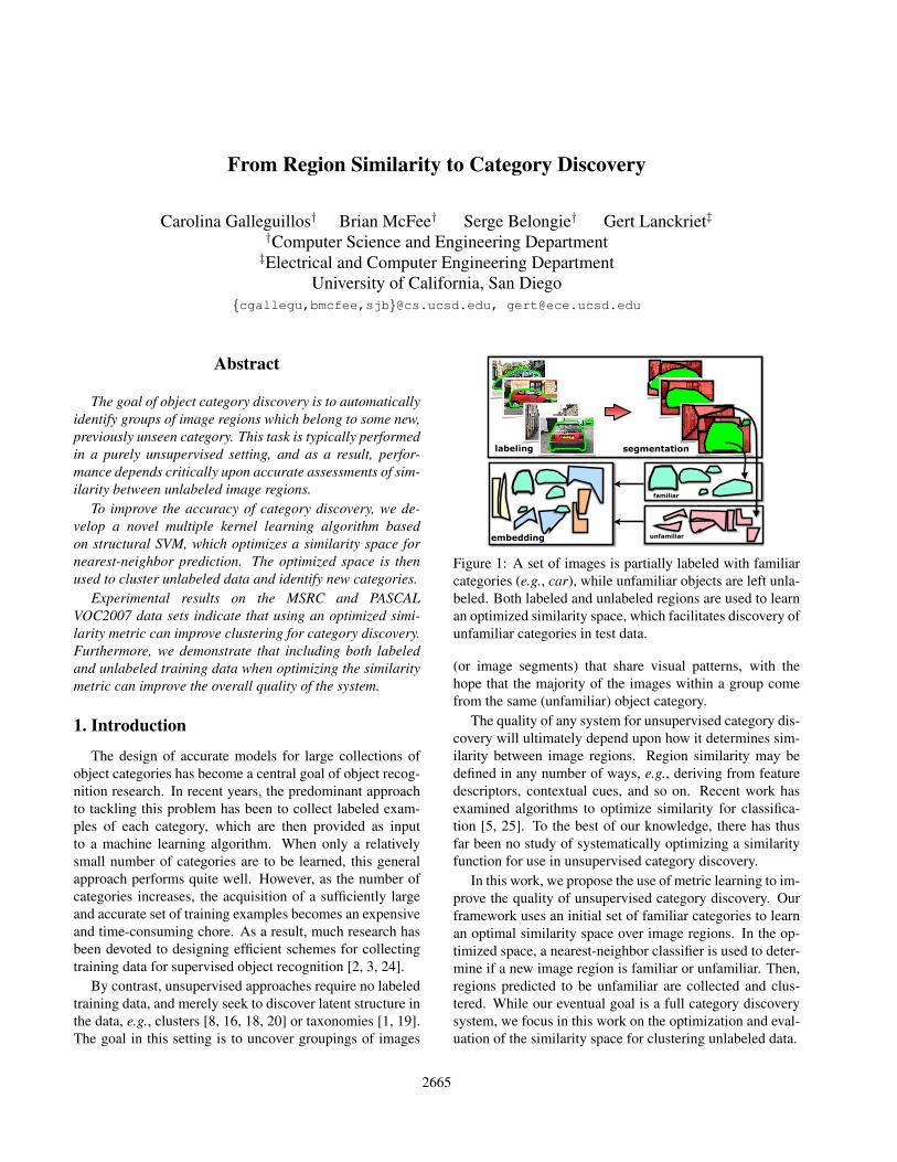
Figure 1: A set of images is partially labeled with familiarcategories (e.g., car), while unfamiliar objects are left unla-beled. Both labeled and unlabeled regions are used to learnan optimized similarity space, which facilitates discovery ofunfamiliar categories in test data.

(or image segments) that share visual patterns, with thehope that the majority of the images within a group comefrom the same (unfamiliar) object category.

The quality of any system for unsupervised category dis-covery will ultimately depend upon how it determines sim-ilarity between image regions. Region similarity may bedefined in any number of ways, e.g., deriving from featuredescriptors, contextual cues, and so on. Recent work hasexamined algorithms to optimize similarity for classifica-tion [5, 25]. To the best of our knowledge, there has thusfar been no study of systematically optimizing a similarityfunction for use in unsupervised category discovery.

In this work, we propose the use of metric learning to im-prove the quality of unsupervised category discovery. Ourframework uses an initial set of familiar categories to learnan optimal similarity space over image regions. In the op-timized space, a nearest-neighbor classifier is used to deter-mine if a new image region is familiar or unfamiliar. Then,regions predicted to be unfamiliar are collected and clus-tered. While our eventual goal is a full category discoverysystem, we focus in this work on the optimization and eval-uation of the similarity space for clustering unlabeled data.

2665

1.1. Our Approach: Improving Similarity

In our framework, we assume that a set of training im-ages has been partially annotated with a set of known, fa-miliar categories, so that all image regions correspondingto familiar categories have been labeled (Figure 1). All re-maining, unlabeled image regions are assumed to belong tounfamiliar categories.

Because we do not know to which unfamiliar categoryan unlabeled training image region may belong, we cannotdirectly optimize a similarity function for unfamiliar cate-gories. Instead, we train a similarity metric to discriminatebetween familiar categories by k-nearest-neighbor predic-tion. Our decision to optimize for nearest neighbor accuracyis motivated by two ideas: first, improving nearest neighborclassification provides a direct way to predict if a test seg-ment belongs to a familiar or unfamiliar category, and sec-ond, a metric optimized to discriminate familiar categoriesshould generalize to discriminate unfamiliar categories.

Moreover, because our framework is built upon nearest-neighbor classification, it is inherently multi-class, and au-tomatically extends to novel classes. It can therefore be eas-ily integrated in a continuous learning system with no needretrain each time a new category is discovered.1 We see thisas a key advantage over previous methods, where the de-tection of unfamiliar categories derives from the output ofbinary classifiers trained on familiar categories [13].

Our main technical contribution is a multiple-kernel ex-tension to the metric learning to rank algorithm, which willallow us to learn an optimized similarity space from multi-ple, heterogeneous input features. Our experimental resultsdemonstrate that learning similarity from labeled data canprovide significant improvements over purely unsupervisedmethods. Finally, we show that including unfamiliar dataduring training improves the quality of the learned similar-ity space.

2. Discovering Object ClassesBefore describing our framework in more detail, we will

first introduce notation and formalize the problem.Using ground truth label information (e.g., masks or

bounding boxes), each training image I is partitioned intosegments xi. Each segment xi belongs to exactly one objectof class `i ∈ L, where L is the set of familiar object labels.The set Xm contains all training segments xi derived fromground truth annotations across all images.

Additionally, we partition each training image I intooverlapping regions by running a segmentation algorithmmultiple times. Only those segments that overlap more than50% with a ground truth mask corresponding to a famil-iar label in L are collected into the set Xf. The rest of the

1Although one may expect to improve accuracy by re-training after thediscovery of a new category, in our framework, this step is purely optional.

segments, which lack (familiar) ground truth labels, are col-lected in the set Xu. Throughout, we will refer to segmentscorresponding to familiar classes (i.e., Xm and Xf) as fa-miliar segments, and segments corresponding to unfamiliarlabels (Xu) as unfamiliar segments.2

All segments derived from training images are collectedto form the training set X = Xm ∪ Xf ∪ Xu. Althoughincluding Xf and Xu introduces some noise into the system,we demonstrate empirically in Section 4.3.1 that doing soduring training improves the quality of the final similaritymetric.

For each segment xi ∈ X , we compute several types offeatures φt(xi), where each feature type φt corresponds toa space characterized by a kernel function

kt(xi, xj) = 〈φt(xi), φt(xj)〉 .

From a collection ofm feature spaces over n training points,we will learn a unified similarity metric which is optimizedfor nearest neighbor classification.

At test time, object class discovery proceeds as follows(illustrated in Figure 2). A collection of test images I ′are segmented multiple times to form the test set X ′. Foreach x′ ∈ X ′, we use the optimized metric to locate its k-nearest neighbors from the training set, and a label for x′

is predicted by the majority vote of its neighbors. Unla-beled training segments vote for a synthetic label `0, takento mean unfamiliar.

After classifying each x′ ∈ X ′, all segments with pre-dicted label `0 are used as input to a clustering algorithm.We use spectral clustering [15] with affinities defined by aradial basis function (RBF) kernel on the learned distances:

Aij = exp(−d(x′i, x

′j)/2σ

2),

where d(x′i, x′j) is the squared distance between two test

segments x′i and x′j in the optimized space, and σ is a band-width parameter.

Since our objective here is to produce a more accuratesimilarity space for discovery, we perform our evaluationwith respect to the clustering of (predicted) unfamiliar testsegments. In practice, one would follow this step by anno-tating the cluster with a (likely new) category label, but thisstep is beyond the scope of this paper.

3. Optimizing the SpaceThe first step of our framework consists of learning an

optimized similarity function over image regions. Note thatwe cannot know a priori which features will be discrimina-tive for unfamiliar categories. We therefore opt to includemany different descriptors, capturing texture, color, scene-level context, etc. (See Section 4.1.) In order to effectively

2Familiarity refers to a segment’s true label, which may or may not beavailable: an unlabeled or test segment may be familiar or unfamiliar.

2666

...testimages

multiplesegmentations

imagesegments

featurespace

optimizedspace

classification segmentsassigned

to familiar classes

unfamiliarsegments

clusteringnew

objectcategories

x'ϕ2

...

ϕ1

ϕm

Figure 2: Discovering object classes: Each test image is partitioned into multiple segments, each of which are mappedinto multiple kernel induced feature spaces, and then projected into the optimized similarity space learned by MKMLR(Algorithm 2). Each segment is classified as belonging to a familiar or unfamiliar class by k-nearest-neighbor. Unfamiliarsegments are then clustered in the optimized space, enabling the discovery of new categories.

integrate heterogeneous features, we turn to multiple kernellearning (MKL) [12]. While MKL algorithms have beenwidely applied in computer vision applications [22, 23],most research has focused on binary classifiers (i.e., sup-port vector machines), with relatively little attention givento the optimization of nearest neighbor classifiers.

Recently, multiple kernel large margin nearest neighbor(MKLMNN) has been proposed as a method for integratingheterogeneous data in a nearest-neighbor setting [6]. Likethe original LMNN algorithm [26], MKLMNN attempts tofind a linear projection of data such that each point’s targetneighbors (i.e., those with similar labels) are drawn closerthan dissimilar neighbors by a large margin. While this no-tion of distance margins is closely related to nearest neigh-bor prediction, it does not optimize for the actual nearestneighbor accuracy.

Instead, we will derive a multiple kernel extension of themetric learning to rank algorithm (MLR) [14], which opti-mizes nearest neighbor retrieval more directly by examiningthe ordering of points generated by the learned metric. Be-fore deriving the multiple kernel extension, we first brieflyreview the MLR algorithm for the linear case.

3.1. Metric Learning to Rank

Metric learning to rank (MLR, Algorithm 1) [14] is ametric learning extension of the Structural SVM algorithmfor optimizing ranking losses [10, 21]. Whereas SVMstruct

learns a vectorw ∈ Rd, MLR learns a positive semi-definitematrix W (denoted W � 0) which defines a distance

dW (i, j) = ‖i− j‖2W = (i− j)TW (i− j).

MLR optimizes W by evaluating the quality of rankingsgenerated by ordering the training data by increasing dis-tance from a query point. Ranking quality may be evaluatedand optimized according to any of several metrics, includ-ing precision-at-k, area under the ROC curve, mean averageprecision (MAP), etc. Note that k-nearest neighbor accu-

Algorithm 1 Metric Learning to Rank [14]Input: data X = {x1, x2, . . . , xn} ⊂ Rd,

true rankings y∗1 , y∗2 , . . . y

∗n,

slack trade-off C ≥ 0Output: d× d matrix W � 0

minW�0, ξ

tr(W ) +C

n

∑x∈X

ξx

s. t. ∀x ∈ X , ∀y ∈ Y :〈W,ψ(x, y∗x)〉 ≥ 〈W,ψ(x, y)〉+ ∆(y∗x, y)− ξx

racy can also be interpreted as a performance measure overrankings induced by distance.

Although ranking losses are discontinuous and non-differentiable functions over permutations, SVMstruct andMLR resolve this issue by encoding constraints for eachtraining point as listed in Algorithm 1. Here, X is the train-ing set of n points, Y is the set of all possible rankings(i.e., permutations of X ), y∗x is the true or best ranking3 forx ∈ X , ∆(y∗x, y) is the loss incurred for predicting y insteadof y∗ (e.g., decrease in precision-at-k), and ξx is a slackvariable. 〈W,ψ(x, y)〉 is the score function which evaluateshow well the model W agrees with the input-output pair(x, y), encoded by the feature map ψ.

To encode input-output pairs, MLR uses a variant of thepartial order feature [10] adapted for distance ranking:

ψ(x, y) =∑

i∈X+x , j∈X−x

yijD(x, i)−D(x, j)|X+x | · |X−x |

(1)

D(x, i) = −(x− i)(x− i)T.

Here, X+x and X−x ⊆ X denote the sets of positive and

negative results with respect to example x (i.e., points of

3In this setting, a true ranking is any ranking which places all relevantresults before all irrelevant results.

2667

the same class or different class), and

yij =

{+1 if i preceeds j in y−1 if j preceeds i in y

.

With this choice of ψ, the rule to predict y for a test pointx is to simply sort i ∈ X in descending order of

〈W,D(x, i)〉 = −〈W, (x− i)(x− i)T〉 = −‖x− i‖2W . (2)

Equivalently, sorting by increasing distance ‖x− i‖Wyields the ranking needed for nearest neighbor retrieval.

Although Algorithm 1 lists exponentially many con-straints, cutting-plane techniques can be applied to quicklyfind an approximate solution [11].

3.2. Multiple Kernel Metric Learning

The MLR algorithm, as described in the previous sec-tion, produces a linear transformation of vectors in Rd.In this section, we first extend the algorithm to supportnon-linear transformations via kernel functions, and then tojointly learn transformations of multiple kernel spaces.

Kernel MLR

Typically, non-linear variants of structural SVM algorithmsare derived by observing that the SVMstruct dual programcan be expressed in terms of the inner products (or ker-nel function) between feature maps: 〈ψ(x1, y1), ψ(x2, y2)〉.(See, e.g., Tsochantaridis, et al. [21].) However, to preservethe semantics of distance ranking (Equation 2), it would bemore natural to apply non-linear transformations directly tox while preserving linearity in the structure ψ(x, y). Wetherefore take an alternative approach in deriving kernelMLR, which is more in line with previous work in non-linear metric learning [7, 6].

We first note that by combining Equations 1 and 2 andexploiting linearity of ψ, the score function can be ex-pressed in terms of learned distances:

S(W,x, y) = 〈W,ψ(x, y)〉

=∑

i∈X+x ,j∈X−x

yij‖x− j‖2W − ‖x− i‖2W

|X+x | · |X−x |

. (3)

Let φ : X → H denote a feature map from X to a repro-ducing kernel Hilbert space (RKHS) H. Inner products inH are computed by a kernel function

k(x1, x2) = 〈φ(x1), φ(x2)〉H .

Let L : H → Rn be a linear operator on H which will de-fine our learned metric, and let ‖L‖HS denote the Hilbert-Schmidt operator norm4 of L.

4The Hilbert-Schmidt norm is a natural generalization of the Frobeniusnorm. For our purposes, this can be understood as treating L as a collectionof n elements vi ∈ H (one per output dimension of L), and summing overthe squared-norms ‖L‖HS =

pPi〈vi, vi〉H.

Next, we define a score function in terms of L, which, asin Equation 3, compares learned distances:

SH(L, x, y) =∑

i∈X+x , j∈X−x

yijdL(x, j)− dL(x, i)|X+x | · |X−x |

. (4)

dL(x, i) = ‖L(φ(x))− L(φ(i))‖2

We may now formulate an optimization program similar toAlgorithm 1 in terms of L:

L∗ = argminL,ξ

‖L‖2HS +C

n

∑x∈X

ξx s. t. (5)

∀x, y : SH(L, x, y∗x) ≥ SH(L, x, y) + ∆(y∗x, y)− ξx.

The choice of ‖L‖2HS as a regularizer on L allows us toinvoke the generalized representer theorem [17]. It followsthat an optimum L∗ of Equation 5 admits a representationof the form

L∗ = MΦT,

where M ∈ Rn×n, and Φ ∈ Hn contains the training set infeature space: Φx = φ(x). By defining W = MTM andK = ΦTΦ, we observe two facts:

‖L∗(φ(x)− φ(i))‖2 = ‖MΦTφ(x)−MΦTφ(i)‖2

= ‖Kx −Ki‖2MTM

= ‖Kx −Ki‖2W , (6)

and ‖L∗‖2HS = tr(ΦMTMΦT

)= tr (WK) , (7)

where for any z,Kz = ΦTφ(z) = [k(x, z)]x∈X is a columnvector of the kernel function evaluated at a point z and alltraining points x.

Note that the constraints in Equation 5 render theprogram non-convex in L, which may itself be infinite-dimensional and therefore impossible to optimize directly.However, by substituting Equation 6 into Equation 4, we re-cover a score function of the same form as Equation 3, ex-cept with x, i and j replaced by their corresponding kernelvectors Kx, Ki and Kj . We may then define the kernelizedmetric partial order feature:

ψK(x, y) =∑

i∈X+x , j∈X−x

yijDK(x, i)−DK(x, j)|X+x | · |X−x |

(8)

DK(x, i) = −(Kx −Ki)(Kx −Ki)T.

Thus, at the optimum L∗, the score function can be repre-sented equivalently as

SH(L∗, x, y) = 〈W,ψK(x, y)〉. (9)

Taken together, Equations 7 and 9 allow us to re-formulateEquation 5 in terms of W and K, and obtain a convex op-timization similar to Algorithm 1. The resulting programmay be seen as a special case of Algorithm 2.

2668

Multiple Kernel MLR

To extend the above derivation to the multiple kernel set-ting, we must first define how the kernels will be combined.LetH1,H2, . . . ,Hm each denote an RKHS, each equippedwith corresponding kernel functions k1, k2, . . . , km andfeature maps φ1, φ2, . . . , φm. From each spaceHt, we willlearn a corresponding linear projection Lt. Each Lt willproject to a subspace of the output space, so that each pointx is embedded according to

x 7→ {φt(x)}mt=1 7→ [Lt(φt(x))]mt=1 ∈ Rnm,

where [·]mt=1 denotes the concatenation of projectionsLt(φt(x)). The (squared) Euclidean distance between theprojections of two points x and j is

dM(x, j) =m∑t=1

‖Lt(φt(x))− Lt(φt(j))‖2. (10)

If we substitute Equation 10 in place of dL in Equation 4,we can define a multiple-kernel score function SMKL. Bylinearity, this can be decomposed into the sum of single-kernel score functions:

SMKL ({Lt}, x, y) =∑

i∈X+x , j∈X−x

yijdM(x, j)− dM(x, i)|X+x | · |X−x |

=m∑t=1

SHt(Lt, x, y). (11)

Again, we formulate an optimization problem as in Equa-tion 5 by regularizing each Lt independently:

min{Lt},ξ

m∑t=1

‖Lt‖2HS +C

n

∑x∈X

ξx s. t. (12)

∀x, y : SMKL({Lt} , x, y∗x) ≥ SMKL({Lt} , x, y)+ ∆(y∗x, y)− ξx.

The representer theorem may now be applied indepen-dently to each Lt, yielding L∗t = MtΦT

t . We define posi-tive semi-definite matrices W t = MT

t Mt specific to eachkernel Kt = ΦT

t Φt. Similarly, for kernel Kt, let ψKt be asin Equation 8. Equations 9 and 11 show that, at the opti-mum, SMKL decomposes linearly into kernel-specific innerproducts:

SMKL ({L∗t }, x, y) =m∑t=1

〈W t, ψKt (x, y)〉. (13)

We thus arrive at the Multiple Kernel MLR program(MKMLR) listed as Algorithm 2. Algorithm 2 is a linearprogram over positive semi-definite matrices W t and slackvariables ξ, and is therefore convex.

Algorithm 2 Multiple Kernel MLR (MKMLR)Input: Training kernel matrices K1,K2, . . . ,Km,

true rankings y∗1 , y∗2 , . . . y

∗n,

slack trade-off C ≥ 0Output: n× n matrices W 1,W 2, . . . ,Wm � 0

minW t�0, ξ

m∑t=1

tr(W tKt) +C

n

∑x∈X

ξx

s. t. ∀x ∈ X , ∀y ∈ Y :m∑t=1

〈W t, ψKt (x, y∗x)〉 ≥m∑t=1

〈W t, ψKt (x, y)〉

+ ∆(y∗x, y)− ξx

We also note that like the original score function (Equa-tion 3), SMKL is linear in each yij , so the dependency ony when moving from MLR to MKMLR is essentially un-changed. This implies that the same cutting plane tech-niques used by MLR — i.e., finding the most-violated con-straints — may be directly applied in MKMLR withoutmodification.

4. ExperimentsIn this section we evaluate our optimized similarity by:

(i) the accuracy of segment classification for familiar andunfamiliar classes, (ii) how well the similarities betweenintra- and inter-class instances are learned, and (iii) the pu-rity of the clustering performed in the optimized space.

To evaluate the classification and clustering accuracyof the proposed system, we use the MSRC and PAS-CAL 2007 [4] databases. Our selection of these datasetswas motivated by three factors:

(a) Both datasets contain at least 20 categories, multipleobjects per image, and present challenges such as highintra-class, scale and viewpoint variability.

(b) MSRC provides pixel-level ground truth labels for allthe objects in the scene, offering more detailed infor-mation with which we can evaluate our framework.

(c) PASCAL presents ground truth bounding boxes for afew objects in each image, making the problem moredifficult in cases where segments with different labelsfall inside of the bounding boxes. However, this makesthe evaluation more realistic, as bounding boxes are apopular way of labeling objects for recognition tasks.

For experiments with MSRC, we use the same train andtest split as Lee and Grauman [13] (hereafter referred toas LG10), and the object detection split of PASCAL VOC2007 [4]. We adopt three different partitionings of eachdataset into unfamiliar/familiar classes from LG10 for com-parison purposes.

2669

Set Unfamiliar Familiar1 1, 2, 7, 11, 20 3–6, 8–10, 12–19, 21

(a) 2 1–4, 10, 16, 17, 19–21 5–9, 11–15, 183 1–7, 9–11, 13, 16–19 8, 12, 14, 15, 20, 211 1, 3, 10, 14, 20 2, 4–9, 11–13, 15–19

(b) 2 1, 4–6, 9, 11, 14, 15, 17–19 2, 3, 7, 8, 10, 12, 13, 16, 203 4–14, 16, 18–20 1–3, 15, 17

Table 1: Partitions for unfamiliar and familiar classes for (a)MSRC and (b) PASCAL VOC 2007.

MSRC PASCALSet 1 Set 2 Set 3 Set 1 Set 2 Set 3

|L| 16 11 6 15 10 5|Xm| 640 548 322 458 278 174|Xf| 870 583 318 535 321 183|Xu| 261 435 813 180 394 532|X ′f | 4124 3160 2375 583 330 206|X ′u | 1975 2939 3724 200 453 577

Table 2: The number of known categories (L) and trainingand test segments in each partition of the datasets.

The different class partitions are shown in Table 1 andstatistics of each partition are reported in Table 2.

Note that the number of examples in PASCAL VOC 07is smaller than in MSRC. This is because PASCAL imagesmay contain unlabeled regions, and few objects are labeledin each scene. Training segmentations were sub-sampled inorder to preserve balance within the training set with respectto the bounding box regions. We retain only the largest twosegments per object in each image.

4.1. Features

Six different appearance and contextual features werecomputed: SIFT, Self-similarity (SSIM), LAB color his-togram, PHOG, GIST contextual neighborhoods and LABcolor histogram for Boundary Support. For each featuretype, we apply an RBF kernel over χ2-distances, with pa-rameters set to match those reported in [6].

4.2. Implementation

The implementation uses the 1-slack margin-rescalingcutting plane algorithm [11] to solve for allW t within a pre-scribed tolerance ε = 0.01. We further constrain each W t

to be a diagonal matrix. This simplifies the semi-definiteprogram to a linear program. For m kernels and n trainingpoints, this also reduces the number of parameters neededto learn from O(mn2) (m symmetric n-by-n matrices) tomn.

In all experiments with MKMLR, we choose the rank-ing loss ∆ as the normalized discounted cumulative gain(NDCG) [9] truncated at 10. Slack parameters C and kernelbandwidth σ for spectral clustering were found by cross-validation on the training set. For testing, we fix k = 17as the number of nearest neighbors for classification acrossall experiments. Multiple stable segmentations were com-puted — 9 different segmentations for each image — each

Xm Xm ∪ XfTraining subset Set 1 Set 2 Set 3 Set 1 Set 2 Set 3Xm 0.57 0.49 0.14 0.65 0.64 0.14Xm ∪ Xf 0.64 0.48 0.72 0.68 0.63 0.80Xm ∪ Xf ∪ Xu 0.65 0.56 0.72 0.68 0.66 0.80

Table 3: Classification accuracy achieved for various train-ing subsets of MSRC, and retrieval sets Xm or Xm ∪ Xf.

of which contains between 2 and 10 segments, resulting in54 segments per image [6].

4.3. Classification accuracy

In order to evaluate the quality of our similarity space,we perform two different classification experiments: one tomeasure the benefits of training with unlabeled data whenpredicting familiar classes, and another to assess the accu-racy of predicting if a test segment is familiar or not, and ifso, its correct label.

4.3.1 The benefits of unlabeled data

Unlabeled data could potentially introduce noise to the met-ric learning step. Therefore, to objectively evaluate the con-tributions of labeled and unlabeled data during training, weevaluate classification accuracy by training metrics on threesubsets of the training data: familiar regions (Xm), familiarregions and segments (Xm ∪ Xf), and all training segments(Xm ∪ Xf ∪ Xu). Due to its dense region labeling, we focuson the MSRC dataset for this experiment. We restrict thetest set to only familiar classes, and repeat the experimentfor each partition of classes.

We also vary which subset of training data is used toform nearest-neighbor predictions — the retrieval set — attest time: either just Xm, or Xm ∪ Xf. This allows us toevaluate the impact on accuracy due to auto-segmentationof training images.

Table 3 illustrates that including both Xf and Xu duringtraining provides significant improvements in test-set accu-racy. Similarly, includingXf in the retrieval set at predictiontime also provides substantial boosts in performance. Thisis likely due to the fact that test images are automaticallysegmented, and Xf provides examples closer in distributionto the test set.

4.3.2 Classification of unfamiliar segments

We evaluate our learned similarity space by computing clas-sification accuracy over the full test set (X ′f ∪X ′u). For eachpartition (Set 1,2,3) of MSRC and PASCAL, we train a met-ric with MKMLR on the entire training set. For comparisonpurposes, we repeat the experiment on metrics learned byMKLMNN, as well as the “native” feature spaces formedby taking the unweighted combination of base kernels. Attest time, a segment is predicted to belong either to one of

2670

Algorithm Set 1 Set 2 Set 3Native 0.51 0.59 0.71

MSRC MKLMNN 0.61 0.57 0.69MKMLR 0.62 0.61 0.72Native 0.31 0.58 0.74

PASCAL07 MKLMNN 0.32 0.51 0.67MKMLR 0.33 0.54 0.70

Table 4: Nearest-neighbor classification accuracy ofMKMLR, MKLMNN, and the native feature space, includ-ing `0.

the familiar classes L, or the unfamiliar class `0. The over-all accuracy is reported in Table 4.

When there are fewer familiar classes from which tochoose, the problem becomes easier because more test seg-ments must belong to the unfamiliar class. This trend isdemonstrated by the increasing accuracy of each algorithmfrom Set 1 (5 unfamiliar classes) to Set 2 (10 unfamiliar)and Set 3 (15 unfamiliar).

In MSRC, where image regions are densely labeled, weobserve that MKMLR consistently outperforms MKLMNNand the native space, although the gap in performance islargest when more supervision is provided. On PASCAL,however, we observe that the unweighted kernel combina-tion achieves the highest accuracy for Sets 2 and 3, i.e., thesets with the least supervision. This may be attributed toMKLMNN and MKMLR over-fitting the training set, whichfor PASCAL is considerably smaller than that of MSRC(see Table 2).

4.4. Intra-class versus Inter-class affinities

Our second evaluation replicates an experiment onMSRC Set 1 in LG10 (Table 1, [13]). A distance matrixis computed for all pairs of test segments predicted to beunfamiliar by the segment classification step. Then, usingthe ground-truth labels, the average precision is computedfor each test segment. Finally, the MAP score is computedfor all unfamiliar classes.

Relying on the segment classification step to determinewhich points are familiar and unfamiliar may introduce biasto the evaluation. We therefore repeat the above experimentusing ground-truth familiar and unfamiliar labels. Table 5shows the MAP results for both experiments. For complete-ness, we again compare the performance of MKMLR toMKLMNN [6]. 5

We observe in the unbiased evaluation (Table 5b) thatMKMLR outperforms the other methods under considera-tion for all categories.

4.5. Cluster purity

Our final evaluation concerns the purity of clusters dis-covered in the test data. Again, we compare the native (un-

5In Table 5, MKLMNN has no MAP score for class tree because therewas only one test segment of that class predicted as unfamiliar.

Airplane Bicycle Building Cow Tree(a) [13] 0.36 0.21 0.32 0.41 0.36

MKLMNN 0.75 0.51 0.38 0.71 -Native 0.61 0.37 0.30 0.40 0.49Ours 0.84 0.58 0.38 0.41 0.70

(b) MKLMNN 0.68 0.50 0.44 0.59 0.59Native 0.65 0.43 0.33 0.36 0.57Ours 0.81 0.55 0.45 0.71 0.66

Table 5: Comparison of MAP scores for Set 1 in MSRC. (a)MAP for segments predicted to be unfamiliar. (b) MAP ontrue unfamiliar segments. Test segments are correctly clas-sified as familiar with 95% accuracy and unfamiliar with54% accuracy.

weighted) kernel combination, MKLMNN, and MKMLRon each partition of MSRC and PASCAL. For each set, wereplicate the experiment of LG10 (Figure 5, [13]), and us-ing the ground-truth labels, perform spectral clustering inthe optimized space on the test segments belonging to unfa-miliar classes. We vary the number of clusters c ∈ [2, 35],and for each c, compute the average purity of the clustering,where a cluster B’s purity is defined as

purity(B) = max`∈L|{x′ ∈ B ∧ `(x′) = `}| /|B|.

For each value of c, we generate 10 different clusterings,and report the average purity. The resulting mean puritycurves are reported in Figure 3.

We observe that in all cases, the mean purity achievedby MKMLR is consistently above that of the native space(almost always significantly so), and is often significantlyabove that achieved by MKLMNN.

The reduced purity scores for PASCAL (relative toMSRC) can be attributed to two facts. First, the sparsity ofground truth labels in PASCAL indicates that the evaluationhere is somewhat less thorough than for MSRC. Second, asdescribed in Section 4.3.2 , the reduced size of the trainingset leads to some overfitting by both MKLMNN andMKMLR. However, while in Section 4.3.2 we observed adecrease in classification accuracy (compared to the nativespace), here we observe an increase in cluster purity. Thisindicates that MKMLR is learning some useful informationwhich is not directly reflected in classification accuracy.

5. ConclusionWe have introduced a novel framework for improving

object class discovery. By optimizing similarity by learningfrom a set of familiar category labels, we are able to moreaccurately cluster unlabeled test data. We also show thatincluding unlabeled data during training can significantlyimprove the quality of the learned space. In future work,we intend to integrate this system with an active learningframework, to continuously explore large sets of object cat-egories.

2671

0 5 10 15 20 25 30 35 400

0.1

0.2

0.3

0.4

0.5

0.6

0.7

0.8

0.9

1Purity Set 1 Pascal

number of clusters

purity

mklmnn

no learning

mkmlr

0 5 10 15 20 25 30 35 400

0.1

0.2

0.3

0.4

0.5

0.6

0.7

0.8

0.9

1Purity Set 3 Pascal

number of clusters

purity

mklmnn

no learning

mkmlr

0 5 10 15 20 25 30 35 400

0.1

0.2

0.3

0.4

0.5

0.6

0.7

0.8

0.9

1Purity Set 5 Pascal

number of clusters

pu

rity

mklmnn

no learning

mkmlr

0 5 10 15 20 25 30 35 400

0.1

0.2

0.3

0.4

0.5

0.6

0.7

0.8

0.9

1Purity Set 5 MSRC

number of clusters

pu

rity

mklmnn

no learning

mkmlr

0 5 10 15 20 25 30 35 400

0.1

0.2

0.3

0.4

0.5

0.6

0.7

0.8

0.9

1Purity Set 3 MSRC

number of clusters

pu

rity

mklmnn

no learning

mkmlr

0 5 10 15 20 25 30 35 400

0.1

0.2

0.3

0.4

0.5

0.6

0.7

0.8

0.9

1Purity Set 1 MSRC

number of clusters

pu

rity

mklmnn

no learning

mkmlr

Set 1 MSRC : 5 unknowns/ 16 knowns

Pu

rit

y

number of clusters

Set 2 MSRC : 10 unknowns/ 11 knowns

number of clusters

Pu

rit

y

Set 3 MSRC : 15 unknowns/ 6 knowns

number of clusters

Pu

rit

y

Set 1 PASCAL : 5 unknowns/ 15 knowns Set 2 PASCAL : 10 unknowns/ 10 knowns Set 3 PASCAL : 15 unknowns/ 5 knowns

number of clustersnumber of clustersnumber of clusters

Pu

rit

y

Pu

rit

y

Pu

rit

y

MKMLR

Native

MKLMNN

MKMLR

Native

MKLMNN

MKMLR

Native

MKLMNN

MKMLR

Native

MKLMNN

MKMLR

Native

MKLMNN

MKMLR

Native

MKLMNN

Figure 3: Mean cluster purity curves. Top plots correspond to different sets in MSRC, and bottom plots correspond toPASCAL VOC2007. Error bars correspond to one standard deviation. Dashed lines correspond to bounds on purity scoresreported by LG10 (Figure 5e, [13]).

Acknowledgments: C.G. and S.B. are supported by NSFGrant AGS-0941760 and DARPA Grant NBCH1080007subaward Z931303. B.M. and G.R.G.L. are supported byQualcomm, Inc., eHarmony, Inc., and NSF Grant CCF-0830535. This work was supported in part by the UCSDFWGrid Project, NSF Research Infrastructure Grant EIA-0303622.

References[1] E. Bart, I. Porteous, P. Perona, and M. Welling. Unsupervised learn-

ing of visual taxonomies. In CVPR, pages 1 –8, 2008.[2] S. Branson, C. Wah, F. Schroff, B. Babenko, P. Welinder, P. Per-

ona, and S. Belongie. Visual Recognition with Humans in the Loop.ECCV, pages 438–451, 2010.

[3] B. Collins, J. Deng, K. Li, and L. Fei-Fei. Towards scalable datasetconstruction: An active learning approach. ECCV, 2008.

[4] M. Everingham, L. Van Gool, C. K. I. Williams, J. Winn, andA. Zisserman. The PASCAL Visual Object Classes Challenge 2007(VOC2007) Results.

[5] A. Frome, Y. Singer, F. Sha, and J. Malik. Learning globally-consistent local distance functions for shape-based image retrievaland classification. In ICCV, pages 1–8, 2007.

[6] C. Galleguillos, B. McFee, S. Belongie, and G. Lanckriet. Multi-class object localization by combining local contextual interactions.In CVPR, pages 113–120, 2010.

[7] A. Globerson and S. Roweis. Visualizing pairwise similarity viasemidefinite embedding. In AISTATS, 2007.

[8] K. Grauman and T. Darrell. Unsupervised learning of categories fromsets of partially matching image features. CVPR, 2006.

[9] K. Jarvelin and J. Kekalainen. Cumulated gain-based evaluation ofir techniques. ACM Trans. on Information Systems, 2002.

[10] T. Joachims. A support vector method for multivariate performancemeasures. In ICML, pages 377–384, 2005.

[11] T. Joachims, T. Finley, and C.-N. J. Yu. Cutting-plane training ofstructural svms. Mach. Learn., 77(1):27–59, 2009.

[12] G. R. G. Lanckriet, N. Cristianini, P. Bartlett, L. El Ghaoui, and M. I.Jordan. Learning the kernel matrix with semidefinite programming.JMLR, 5:27–72, 2004.

[13] Y. Lee and K. Grauman. Object-graphs for context-aware categorydiscovery. In CVPR, 2010.

[14] B. McFee and G. Lanckriet. Metric learning to rank. In ICML, 2010.[15] M. Meila and J. Shi. Learning Segmentation by Random Walks.

NIPS, 2001.[16] B. Russell, W. Freeman, A. Efros, J. Sivic, and A. Zisserman. Using

multiple segmentations to discover objects and their extent in imagecollections. In CVPR, 2006.

[17] B. Scholkopf, R. Herbrich, A. J. Smola, and R. Williamson. A gen-eralized representer theorem. In COLT, pages 416–426, 2001.

[18] J. Sivic, B. Russell, A. Efros, A. Zisserman, and W. Freeman. Dis-covering objects and their location in images. In ICCV, 2005.

[19] J. Sivic, B. Russell, A. Zisserman, W. Freeman, and A. Efros. Unsu-pervised discovery of visual object class hierarchies. In CVPR, pages1 –8, 2008.

[20] S. Todorovic and N. Ahuja. Extracting subimages of an unknowncategory from a set of images. In CVPR, 2006.

[21] I. Tsochantaridis, T. Joachims, T. Hofmann, and Y. Altun. Largemargin methods for structured and interdependent output variables.J. Mach. Learn. Res., 6:1453–1484, 2005.

[22] M. Varma and D. Ray. Learning the discriminative power-invariancetrade-off. In ICCV, 2007.

[23] A. Vedaldi, V. Gulshan, M. Varma, and A. Zisserman. Multiple ker-nels for object detection. In ICCV, 2009.

[24] S. Vijayanarasimhan and K. Grauman. What’s it going to cost you?:Predicting effort vs. informativeness for multi-label image annota-tions. In CVPR, 2009.

[25] G. Wang, D. Hoiem, and D. Forsyth. Learning image similarity fromflickr groups using stochastic intersection kernel machines. In CVPR,2010.

[26] K. Q. Weinberger, J. Blitzer, and L. K. Saul. Distance metric learningfor large margin nearest neighbor classification. NIPS, 2006.

2672