DETERMINATION OF CLOUD AND

PRECIPITATION CHARACTERISTICS

FROM SATELLITE, RADAR AND

RAINGAGE ANALYSIS

LP-127

FINAL REPORT

TWDB CONTRACTS NO. 14-90023 AND 14-00004

Prepared by:

DONALD R. HARAGAN

JERRY JURICACOLLEEN A. LEARY

ATMOSPHERIC SCIENCE GROUP

TEXAS TECH UNIVERSITY

LUBBOCK, TEXAS

Prepared for:

TEXAS DEPARTMENT OF WATER RESOURCES

AUSTIN, TEXAS

Funded by:

DEPARTMENT OF THE INTERIOR, BUREAU OF RECLAMATIONTEXAS DEPARTMENT OF WATER RESOURCES

June 1980

MS-230 (3*78)Bureau of Reclamation TECHNICAL REPORT STANDARD TITLE PAGE

t. REPORT NO.

4. TITLE AND SUBTITLE

Final Report of Contract IAC (78-79)2104

7. AUTHOR(S) Donald R. HaraganJerry JuricaColleen A. Leary

9. PERFORMING ORGANIZATION NAME AND ADDRESS

Atmospheric Science GroupTexas Tech UniversityP.O. Box 4320

Lubbock, Texas 7940912. SPONSORING AGENCY NAME AND ADDRESS

Texas Department of Water ResourcesP.O. Box 13087 Capitol StationAustin, Texas 78711

is. supplementary notes Submitted to:

Office of Atmospheric Resources ManagementWater and Power Resources ServiceDenver Federal Center; Box 25007; Denver, Colorado 80225

16. ABSTRACT

5. REPORT DATE

January 1, 1980

6. PERFORMING ORGANIZATION CODE

580/330

8. PERFORMING ORGANIZATIONREPORT NO.

LP-127

10. WORK UNIT NO.

.5540.11. CONTRACT OR GRANT NO.

IAC (78-79) 210413. TYPE OF REPORT AND PERIOD

COVERED

1 January 1979 to31 December 1979

14. SPONSORING AGENCY CODE

Data gathered during the Texas HIPLEX field programs of 1977, 1978and 1979 are analyzed and discussed. Specific data treated are recording ralngage data, digitized radar data and geostationary satelliteradiance data. Individual analyses are presented as well as resultsderived from integration of the several data sources into a more complete case study of certain dates. It is concluded that such integration of individual analyses yields greatly improved understanding ofthe revelant meteorological processes.

17. KEY WORDS AND DOCUMENT ANALYSIS

o. descriptors-- Weather modification/cumulus clouds/meteorological radar/raingafes/geostationary satellite/rainfall/cloud seeding

b. identifiers-- Texas/High Plains/HIPLEX

c. COSATI Field/Group COWRR:

18. DISTRIBUTION STATEMENT

Available from the National Technical Information Service, OperationsDivision. Springfield, Virginia 22161.

19. SECURITY C LASS(THIS REPORT)

UNCLASSIFIED20. SECURITY CLASS

(This page)

UNCLASSIFIED

21. NO. OF PAGES

22. PRICE

GPO 845-630

HIPLEX FINAL REPORT

for the Period

1 January 1979 to 31 December 1979

submitted to

Texas Department of Water Resources

and the

U.S. Department of the Interior

by

Atmospheric Science Group

Texas Tech University

work performed under

Contract IAC(78-79)2104

TDWR Contract No. 14-90023

LP-127

Principal Investigators

Donald R. Haragan

Jerry Jurica

Colleen A. Leary

June 1, 1980

TABLE OF CONTENTS

Abstract iii

List of Figures iv

List of Tables vi

Introduction 1

Work Performed 1

Task 1. Determination of Cloud Propertiesfrom Satellite Data 1

Task 2. Integration of Satellite Datawith Raingage and Radar Measurement 16

Task 3. Rainfall Analysis 35

Task 4. Radar Data Collection for

1979 Field Experiment 53

Task 5. Support to the Field Program 68

References 69

li

ABSTRACT

Data gathered during the Texas HIPLEX field programs of 1977,

1978 and 1979 are analyzed and discussed. Specific data treated

are recording raingage data, digitized radar data and geostationary

satellite radiance data. Individual analyses are presented as well

as results derived from integration of the several data sources into

a more complete case study of certain dates. It is concluded that

such integration of individual analyses yields greatly improved under

standing of the relevant meteorological processes.

in

LIST OF FIGURES

1-1. Location and approximate operational coverage of thetwo satellite data sources. 2

1-2. The area of study. 3

1-3. Variation of percent cloud cover with time. 7

1-4. Curves of the frequency distribution of visibleradiance values on 22 June. 8

1-5. Curves of the frequency distribution of visibleradiance values of 24 June. 9

1-6. Curves of the frequency distribution of visibleradiance values on 27 June. 10

1-7. Curves of the frequency distribution of visibleradiance values on 8 July. 11

2-1. Surface chart at 1800 GMT and 500 mb chart at1200 GMT on 8 July 1977. 17

2-2. Variation of total network precipitation withtime on 8 July 1977. 19

2-3. Precipitation analysis of the total precipitationfrom 1800 GMT 8 July to 0000 GMT 9 July 1977. 20

2-4. PPI displays on 8 July 1977 from the M-33 radarat Snyder. 21

2-5. Cloud albedo, cloud top temperature andrainfall intensity on 8 July 1977. 23

2-6. Isohyet pattern for the period 1945-2000 GMT8 July 1977. 25

2-7. RKI display derived from M-33 radar for theazimuth angle 235° at 1942 GMT 8 July 1977, togetherwith cloud top height derived from satellite infrareddata and actual raingage measurements. 26

2-8. Isohyet pattern for the period 2015-2030 GMT8 July 1977. 28

2-9. RHI display derived from M-33 radar data for theazimuth angle 253° at 2018 GMT 8 July 1977, togetherwith cloud top height derived from satellite infrareddata and actual raingage measurements. 29

2-10. Same as Figure 2-9 for azimuth angle 259 . 31

2-11. Atmospheric soundings taken at Big Spring on8 July 1977. 33

iv

3-1. GOES EAST enhanced infrared satellite photographof the cloud pattern over the Texas HIPLEX areaat 2100 GMT on 8 July 1977. 38

3-2. RHI (a) and low-level (1°) PPI (b) displays derivedfrom Snyder digital radar data for 2104 GMT, 8 July1977. 40

3-3. Temperature (solid line) and dew point (dashed line)at 2100 GMT on 8 July at Post plotted in skew T -log p format. 41

3-4. The 2100 GMT Post sounding from Fig. 3-3 superposedon the lower portions of Zipser's (1977, Fig. 8)collection of soundings in and beneath tropical anvilclouds associated with intense tropical convection. 41

3-5. Surface winds at 2100 GMT on 8 July 1977 superposedon the low-level radar echo pattern of Fig. 3-2b. 42

LIST OF TABLES

1-1. Number of clouds of different sizes 6

1-2. Comparison of percent cloud cover and cloudnumbers from satellite radiance data and

photographic imagery. 13

3-1. HIPLEX radar characteristics Snyder, Texas 1977 36

3-2. Wind direction (degrees) and speed (m s""1) at 2100 GMT 44

3-3. 1977 Precipitation 46

3-4. 1978 Precipitation 48

3-5. 1977 Storm Data 50

3-6. 1978 Storm Data 51

4-1. Skywater radar Texas HIPLEX scanning modes 1979 54

4-2. Inventory of digital radar data. 55

4-3. Inventory of 16mm movie film 63

4-4. Inventory of radar video tapes Summer 1979 66

VI

INTRODUCTION

Since its initiation, the ultimate objective of the Texas HIPLEX

program has been the integration of surface, upper air, radar and satellite

data in a manner beneficial to the proper design and subsequent evaluation

of a rainfall enhancement experiment. The analysis effort at Texas Tech

University during 1979 reflects this integrative approach. Surface rain

fall, radar, and satellite data have been utilized in order to better

define storm rainfall and the mesoscale convective systems responsible.

WORK PERFORMED

Five tasks were undertaken during calendar year 1979.

Task 1. Determination of Cloud Properties from Satellite Data

The principal responsibility of the meteorological satellite support

provided to the 1979 Texas HIPLEX program by Texas Tech has been twofold:

(1) the development of techniques to expand the analysis of data by utiliz

ing satellite measurements, and (2) support of forecasting and aircraft

operations during the summer field program. The data source for the effort

has been visible and infrared radiance measurements and photographic imagery

from the GOES (Geostationary Operational Environmental Satellite) system,

utilizing both GOES-WEST and GOES-EAST data (Figure 1-1). The data analysis

activity has consisted of two related portions: the determination of cloud

properties from satellite data and integration of satellite data with rain

gage and radar data (Task 2). The analysis was performed by Mr. Shih-

Cheng Chao, who conducted the research as a thesis project and has recently

completed all requirements for the M.S. degree in Atmospheric Science.

The direct support to the field program is covered under Task 5.

The accomplishments under Task 1 have been achieved through the analysis

of four case study days selected from the 1977 Texas HIPLEX field season -

22, 24 and 27 June and 8 July 1977. The area of study is shown in Figure 1-2,

These four days were selected because of the availability of good satellite,

raingage and radar data sets. On two days, 8 July and 22 June, substantial

rainfalls occurred; on 24 and 27 June, however, little or no precipitation

was recorded within the raingage network. The objective in this Task was

Figure1-1Locationandapproximateoperationalcoverageofthetwosatellitedatasources:GOESVJESTat135°WandGOESEASTat75°Wlongitude.

Figure 1-2 The area of study. The sector at the center isthe Texas HIPLEX study region.

to derive cloud properties from the satellite data, and then compare and

contrast results between rainfall and non-rainfall days.

The visible radiance data were analyzed with a cloud summary program.

The principal input parameter for each time on the four case study days

was the critical brightness, determined with the ADVISAR, to distinguish

cloud from non-cloud surface. A number of statistical products, such as

mean cloud brightness and variance of cloud brightness, as well as the

cloud size were generated through the cloud summary program. After the

cloud-by-cloud statistics were accumulated, the following comprehensive

information was obtained: (1) percentages of cloud cover and non-cloud area

within the study area; (2) mean brightness values of the total cloud and non-

cloud area; (3) brightness distribution of all data points; (4) distribution

of cloud mean brightness; and (5) distribution of cloud size.

The number of clouds and percent cloud cover was obtained for each

time on the four case-study days. The minimum cloud size of interest in

this study is a cloud of four pixels, equivalent in area to a circular cloud

of about 3.3 km diameter. All the clouds with size equal to or less than

three points were discarded by the cloud summary program. The percent

cloud-coyer over the whole area was obtained as the total of all clouds

defined in this manner.

There were several categories employed to separate clouds according to

their size as follows:

1. Tiny clouds, less than 4 pixels, corresponding to a circular cloud

diameter less than 3.3 km, were neglected here.

2. Isolated convective clouds:

(a) Small clouds, 4 to 7 pixels, with an equivalent diameter between

3.3 km and 4.3 km, usually a fair weather cumulus cloud;

(b) Medium clouds, with 8 to 37 pixels, having an equivalent diameter

between 4.3 km and 10 km, cumulus congestus in most cases;

(c) Large clouds, with 38 to 148 pixels and an equivalent diameter

between 10 km to 20 km, and usually identified as cumulonimbus;

3. Widespread deep convection or stratiform clouds, with more than 148

pixels, corresponding to an equivalent diameter larger than 20 km,

are identified as a widespread deep convective cloud for high mean

brightness or as area of stratiform cloud for low mean brightness.

The cloud populations in various size categories derived from the

cloud summary program are given in Table 1-1. A number of different pat

terns were found to occur. Large numbers of clouds appeared on 24 June

and early on 8 July, with much smaller numbers of clouds on the other two

days. Generally speaking, the number of small and medium isolated convec

tive clouds dominated the total number of clouds. As a result, the numerous "

small and medium isolated clouds of 24 June and early on 8 July led to large

total numbers of clouds at these times. However, the percent cloud cover

was always dominated by the widespread convective and stratiform clouds,

independent of the total cloud nuirber.

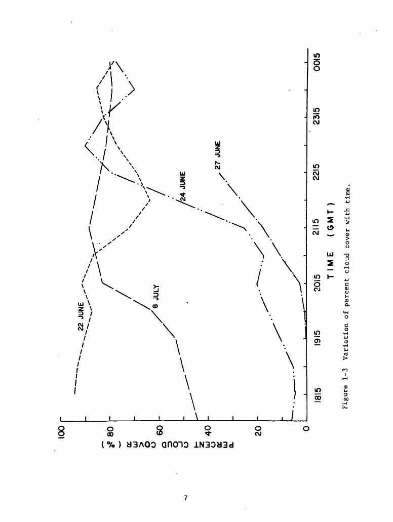
The percent cloud cover was computed as the ratio of the number of

data points within the cloud boundary, determined by the critical visible

value, to the total number of data points within the study area. Figure

1-3 compares the percent cloud cover results over the study area for the

four days. On 22 June, cloud cover exceeded 80% much of the day. Large

percent cloud cover also occurred during the late afternoon of 8 July.

The early afternoon of both 24 and 27 June was dominated by small isolated

clouds, which kept the cloud cover small and even clear for the first four data

times on 27 June. But, on both days in the late afternoon, a storm moved

into the study area from the west, contributing to increased cloud cover over

the study area. Of interest are the contrasting cases of large percent

cloud cover contributed by only a few clouds and small percent cloud cover

despite the presence of many clouds. The cloud cover at 2045 GMT, 22 June

was 87%, although there were only 5 separate clouds at this time. The

percent cloud cover at 1845GMT, 24 June was only 6.1%, despite the presence

of 60 clouds in the study area.

The visible brightness frequency distribution curves for four selected

times at two-hour intervals are shown in Figures 1-4 through 1-7. In each

figure, the abscissa is the difference of individual brightness values

relative to the critical value distinguishing cloud from non-cloud back

ground for the given time. The appearance of the brightness distribution

curves is closely related to the percent cloud cover at the corresponding

time. A comparison between Figure 1-3 and Figures 1-4 through 1-7 shows

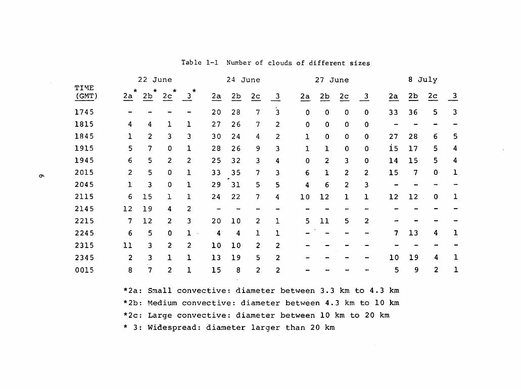
Table 1-1 Nuir.ber of clouds of different sizes

TIME

(GMT)*

2a

22 June

* *

2b 2c*

3 2a

24 June

2b 2c 3 2a

27 June

2b 2c 3 2a

8 July

2b 2c 3

1745 - - - - 20 28 7 3 0 0 0 0 33 36 5 3

1815 4 4 1 1 27 26 7 2 0 0 0 0 - - - -

1845 1 2 3 3 30 24 4 2 1 0 0 0 27 28 6 5

1915 5 7 0 1 28 26 9 3 1 1 0 0 15 17 5 4

1945 6 5 2 2 25 32 3 4 0 2 3 0 14 15 5 4

2015 2 5 0 1 33 35 7 3 6 1 2 2 15 7 0 1

2045 1 3 0 1 29 31 5 5 4 6 2 3 - - - -

2115 6 15 1 1 24 22 7 4 10 12 1 1 12 12 0 1

2145 12 19 4 2 - - - - - - - - - - - -

2215 7 12 2 3 20 10 2 1 5 11 5 2 - - - -

2245 6 5 0 1 4 4 1 1 - - - - 7 13 4 1

2315 11 3 2 2 10 10 2 2 - - - - - - - -

2345 2 3 1 1 13 19 5 2 - - - - 10 19 4 1

0015 8 7 2 1 15 8 2 2 — — — — 5 9 2 1

*2a: Small convective: diameter between 3.3 km to 4.3 km

*2b: Medium convective: diameter between 4.3 km to 10 km

*2c: Large convective: diameter between 10 km to 20 km

* 3: Widespread: diameter larger than 20 km

8

(' .y

•4

III\ y

KV\

\

»//

//

//I

O00

>

5->

00

\

UJz

\\\

8

\

\

UJ

CVl

\

\

O

(%) «3aoo anoio iN30H3d

\

\

/ \\

oCVJ

\

\

JOOo

tn

roCM

in

CVJCM

4J

ID 2 >«._ e> j_!CVJ

*-*' >oa

UJ T31

2 o

o

m I-AJ

o c

CJ a)u

M0)o.

«ho

co

lO •H-^ 4J

0> CO

in

GO

CO>

eni

0)u

•H

CO

5000

4000

u 3000

£3

4J

§ 2000ou

1000

NON-CLOUD REGION

1815 GMT

2015 GMT

2215 GMT

0015 GMT

* CLOUD REGION 4

Figure 1-4 Curves of the frequency distribution of visible radiance values on 22 June

u0

a3

2

4JC3O

U

NON-CLOUD REGION

5000 L

4000 -

3000 -

2000 -

1000 _

CLOUD REGION

1815 GMT

2 015 GMT

2215 GMT

0015 GMT

Figure 1-5 Curves of the frequency distribution of visible radiance values on 24 June.

5-1

.C6

-PC3Ou

Figure

6000-

5000

4000-

3000.

2000-

1000-

NON-CLOUDREGION*•

CLOUDREGION

1745GMT

1915GMT

2045GMT

2215GMT

-56-48-40-32-24-16-3VIS81624324048566472808896crit

1-6Curvesofthefrequencydistributionofvisibleradiancevalueson27June.

uCD

a3Z

•Pc3OU

5000

NON-CLOUD REGION +

4000

3000

2000

CLOUD REGION

174 5 GMT

2 015 GMT

224 5 GMT

0015 GMT

J \ \

v4

I \I \

/ \J \

4

1000 .

/ V\\\

V /j ^ \• !•••••' I I I I 1 1 1 1 1 1 L

-48 -40 -32 -24 -16 -8 VIS 8

crit

16 24 32 40 48 56 64 72 80 88 96

Figure 1-7 Curves of the frequency distribution of visible radiance values on 8 July.

that large cloud cover (greater than 70%) occurred when the mode of the

brightness distribution curve was positive, and that small cloud cover

(less than 45%) corresponded to a negative modal value.

The modal values at 1815 and 2015 GMT on 22 June and 0015 GMT on 23 June

were from 40 to 60 units greater than the critical visible value at those

times and the mode at 2215 GMT was 76 units above the critical value. The

pattern on 8 July had a similar distribution, except for the curve at 1745

GMT, early in the day. The mode at 2015 GMT was 76 units greater than the

critical value, as was also observed at 2215 GMT on 22 June. At all of these

times the total cloud cover was at least 80%. The most substantial rainfalls

observed on the case study days occurred at these times. For both 22 June

and 8 July the visible radiance values in the cloud region of the frequency

distribution curve were skewed toward large positive values.

The patterns for 24 and 27 June are similar, but very different from

those on 22 June and 8 July. On these two days, the brightness frequency

distributions were concentrated in the non-cloud region. The modes at 1815

and 2015 GMT on 24 June were located 32 and 24 units, respectively, below

the corresponding critical values. Late that afternoon, a cloud system

moved into the study area and the pattern of distribution curves at 2215 and

0015 GMT was significantly changed. The patterns on 27 June were all uni

formly concentrated in the non-cloud region, with modal values at the four

selected times all from 40 to 48 units below the critical visible value

for each time. At all of these times, the cloud cover was less than 35%.

In contrast to the 22 June and 8 July curves, the visible radiance values

in the cloud region on 24 and 27 June were quite uniformly distributed over

all positive values. The precipitation analyses from the raingage network

for these four days support the tentative conclusion that the visible data

brightness value distribution curves are correlated with rainfall.

Comparisons of percent cloud cover and cloud numbers derived from

satellite radiance data and from photographic imagery are shown in Table 1-2

at one-hour intervals. Although agreement between the two sets of results

is generally good, there are some instances of poor agreement. In the

original analysis of the photographic imagery, the study area was divided

12

OJ

Table 1-2 Comparison of percent cloud cover and cloud numbers fromsatellite radiance data and photographic imagery.

Percent

Cloud Cover

Ni

Wide

umb

spr

>er

eac

of

I Clouds

Number of

Isolated Clouds

Total Number

of Clouds

DAY

Time

(GMT) Radiance Imagery Rad iance Imagery Radiance Imagery Radiance Imagery

2 2 June 1330 93.5 88 2 1 6.5 42 8. 5 43

1930 89.1 84 1. 5 2 12.5 92 14 94

2030 89.2 81 1 2 5.5 100 6. 5 102

2130 68.3 59 1. 5 1 28.5 105 30 106

2230 73.6 54 2 1 16 37 18 38

2330 - - - - - - - -

23 June 0030 79.3 65 1 1 17 12 18 13

24 June 1730 6.4 32 3 3 55 247 58 250

1830 5.4 9 2 1 59 218 61 219

1930 13.6 23 3. 5 2 61.5 284 65 286

2030 18.7 9 4 2 70 96 74 98

2130 25.4 20 4 3 73 70 77 73

2230 84.8 28 1 2 20.5 27 21. 5 29

2330 76.9 49 2 3 29.5 0 31. 5 3

25 June 0030 78.4 51 2 1 25 5 27 6

Table 1-2 Continued

Percent

Cloud Cover

Number

Widespreadof

Clouds

Numbe

Isolated

r of

Clouds

Total Number

of Clouds

DAY

Time

(GMT) Radiance Imagery Rad iance Imaaery Radiance Imagery Radiance Imagery

27 June 1730 0 0 0 0 0 0 0 0

1830 0 0 0 0 0 0 0 0

1930 0.3 5 1.5 0 2 7 3.,5 7

2030 6.6 5 ' 2.5 1 0. 5 30 13 31

2130 17.8 11 1 1 23 66 24 67

2230 35.2 32 2 2 21 34 23 36

8 July 1730 43.6 57 3 3 74 323 77 326

1830 50.1 53 5 3 61 256 66 259

1930 58.4 61 4 2 35. 5 247 39.,5 249

2030 82.8 73 1 1 22 191 23 192

2130 90.9 79 1 1 24 176 25 177

2230 81.9 83 1 1 24 78 25 79

2330 79.2 70 1 1 33 80 34 81

9 July 0030 80.2 73 1 2 16 73 17 75

into nine sub-areas, as shown in Figure 1-2. In the comparison presented

here, these individual values of percent cloud cover were averaged to pro

duce a more representative overall estimate. Further, the number of isolated

and widespread clouds for the whole study area was obtained by adding the

numbers from each sub-area. Table 1-2 compares the percent cloud cover and

cloud number results derived from these two sources.

The agreement of percent cloud cover between the two sets is good,

except for a few cases on 24 June. Because the percent cloud cover from

photographic imagery was estimated visually, it was difficult to maintain as

consistent an accuracy as with percent cloud cover derived from radiance

data. In general, the difference in percent cloud cover estimated from

these two data sets was approximately 5% to 10%. the most difficult esti

mates of percent cloud cover occurred at times when isolated, cluster or

line clouds were predominant. This situation was particularly true on 24

June, where the differences in Table 1.-2 are very noticeable.

The agreement in Table 1-2 in number of widespread clouds between these

two data sets is seen to be much better than that for isolated clouds.

Especially on 24 June, when isolated clouds dominated, the agreement was

very poor. A detailed study of the results on this date points to an ex

planation. The computer cloud summary program treated many small clouds as

a single large cloud as long as the individual clouds were linked together

at even one point. As a result, the number of widespread clouds was one or

two more than the value derived from the imagery, while the number of isolated

clouds was much less than that from imagery. Early on 8 July, the number

of isolated clouds differed for the same reason, although the numbers of

the widespread clouds were nearly equal.

Another factor influencing the accuracy of these results was the varia

tion in solar zenith angle, which increased to 50 after 2230 GMT; conse

quently, the brightness of the scene was significantly reduced. Under these

conditions, fewer small isolated clouds could be distinguished from the

underlying surface in the photographic imagery. The late afternoons of

24 June and 8 July are good examples of this problem.

15

In conclusion, the results derived from radiance data analyzed by the

summary program are considered to be more accurate and quantitative. How

ever, analysis of the imagery can be of assistance to the study of radiance

data sets, especially in providing a large-scale view of the overall synoptic

pattern existing at a given time.

Task 2. Integration of Satellite Data with Raingage and Radar Measurements

The satellite-derived cloud properties derived in Task 1 have been

compared with raingage and radar data in an effort to establish the re

liability of the satellite results. All four case study days were treated;

however, the presentation here will be limited to a single day, 8 July.

A complete discussion of the four case study days will be given in a tech

nical report to be submitted in the near future. Utilizing the available

satellite, radar and precipitation data, a comparison was made by placing the

three different data sources into a common coordinate system. The reference

coordinates have been selected to be the rectangular array of visible satel

lite radiance measurements used in this study. The objective of this com

parison was to enhance understanding of (a) the structure of the convective

clouds (b) the relation between organized mesoscale features and the synoptic

scale (c) storm development processes, and (d) precipitation mechanisms.

Two weak cold fronts extended from the northeastern United States

through the central United States into Texas at 1500 GMT on 8 July 1977.

The cold fronts moved slowly eastward and passed through the study area at

1800 GMT, just before heavy rainfall was detected in the raingage network

(Figure 2-1). During the next three-hour interval, the fronts moved east

ward and left the study area by 0000 GMT 9 July, as the rainfall subsided.

A distinct ridge and trough pattern was present at 500 mb on 8 July.

The ridge passed through the New Mexico area at 1200 GMT and remained sta

tionary until 0000 GMT 9 July. Cold air advection occurred within the study

area at the 500 mb level.

The recording raingage network in 1977 consisted of 59 stations and

recorded rainfall to the nearest one-hundredth inch for every 15-minute

16

Figure 2-1 Surface chart at 1800 GMT and 500 mb chart at1200 GMT on 8 July ]977.

17

interval. The precipitation analysis indicated that the precipitation on

8 July was concentrated in the afternoon, from 1830 to 2045 GMT, when a line

of intense rainfall formed in association with the passage of the two cold

fronts through the raingage network. The rain subsided within the raingage

network soon after the cold fronts moved out of the study area. The varia

tion with time of total precipitation volume on 8 July is shown in Figure 2-2.

The value plotted at a given time represents the rainfall occurring during

the preceding 15-minute interval. The spatial pattern of total rainfall

from 1800 to 0000 GMT 9 July (Figure 2-3) shows that the heavy rainfall areas

were located in a band stretching from southwest to northeast, with many

stations collecting over 1.5 inches during this six-hour interval. The

broken isohyet in Figure 2-3 represents a rainfall of 0.01 inch and the

solid contours are given for every 0.25 inch. The total surface water

produced by precipitation was found to be 66,095 acre-ft, the heaviest rain

among the four case study days.

The highly modified M-33 radar located at Winston Field in Snyder,

Texas, provided the digital data for this case study day. Figure 2-4

shows PPI plots from the M-33 radar on 8 July 1977. The borders of the

raingage network and satellite study area are drawn over the radar echo

pattern. The plot for 1948 GMT shows that a cluster of strong reflectivity

cells located in the central portion of the raingage network passed through

the Snyder area, although no data were available within 25 km of the radar

site because of the range delay. The rainfall pattern during the period

1930-1945 GMT verified that a heavy rain band passed through this area,

producing more than 0.80 inch within 15 minutes at two stations. The rain

band structure persisted until 2018 GMT, maintaining the same appearance

in the precipitation pattern. The rainfall intensity decreased rapidly after

2015 GMT, although the rainfall area remained in the central portion of the

raingage network. The PPI plots show that the echo area became more wide

spread later, but that reflectivity values weakened. The precipitation

analysis and digital PPI plots were in good agreement on this point. The

satellite visible data showed increases in the percent cloud cover and in

the area covered by the brightest clouds early in the study period, reaching

maximum values near 2015 GMT, as was observed in the precipitation pattern.

18

10

9 -

i

<D

§ 8

o

~ 7

UJ

O>

o

§Q.

LUtrQ.

I I I

1900

.j I J L I I I

2000 2100

TIME (GMT)

J L

2200

Figure 2-2 Variation of total network precipitationwith time on 8 July 1977.

19

101.8 101.6 101.4 1012

LONGITUDE

1010 100.8

Figure 2-3 Precipitation analysis of the total precipitationfrom 1800 GMT 8 July to 0000 GMT 9 July 1977.The isohyets are labelled in inches.

20

100.6

I9>41l I

I « NO«•« rt:

T |.*TMl4t« II4>«tl*4

Figure 2-4 PPI displays on 8 July 1977 from the M-33 radarat Snyder. The outer boundary shows the studyarea, while the inner box is for the raingagenetwork. The echo threshold is 25 dBz and dark

solid areas represent reflectivities greaterthan 45 dBz.

21

948 GMT

The latitude and longitude coordinates of each raingage station have

been located in the satellite radiance data arrays. After plotting the rain

gage data, isohyetal patterns were constructed in the transformed coordinate

system for comparison with the radiance data. Note that the reference

coordinate system was selected to be the rectangular array of visible satel

lite radiance data.

The rain began in the interval 1830-1845 GMT, as was shown in Figure

2-2. The sequence of diagrams in Figure 2-5 shows the relative location

of cloud albedo, cloud top temperature and the rain area. Note that only

the coldest isotherms are shown in any given frame in Figure 2-5. The

diagram at 1845 GMT shows that the most intense rain area was located under

the brightest and coldest cloud tops within which the cloud albedo was larger

than 0.63 and the corresponding cloud top height was above 13 km. More than

0.5 inch of rain had occurred within the previous 15 minutes. A strong rain

band along a line from Snyder to Big Spring formed soon after the rain began,

and is the rain band detected in the PPI radar plots of Figure 2-4. The

maximum precipitation occurring within the rain band was located under clouds

with either high albedo or high tops, or both. The rainfall intensity increased

sharply after 1915 GMT when the clouds over the raingage network developed

tops to approximately 14.5 km and the area of albedo greater than 0.63

increased considerably. The precipitation peak was reached just before

2000 GMT. Meanwhile, at 2015 GMT the raingage network was totally covered

by bright and high-topped clouds with albedos over 0.63 and top heights

above 15 km. The PPI digital radar analysis also indicated that the reflec

tivity gradients within the rain band became quite sharp, attaining values

greater than 55 dBz at this time. The rainfall intensity decreased rapidly

after the precipitation peak and little precipitation was recorded after

2130 GMT.

Three RHI plots for 1942 GMT were taken along the azimuth angles 200°,

235 , and 242 with respect to Snyder. Figure 2-6 shows the isohyet pattern

for the period 1945-2000 GMT, upon which lines are drawn marking the three

cross sections investigated. The cross section along the line BB1 in Figure

2-6 contained intense reflectivity values, as evidenced by a raingage mea

surement at 32 km range of 0.80 inch within 15 minutes (Figure 2-7). Cross

22

o ^>

1845 GMT

£?•

PST

MAF Sjj "^5/

Albedo

0.44

0.63

Cloud-top temperature (C)

-40^.-49

-50--59

-60—69

Rainfall ( inch/15 min )

0.01-0.09 I J0.10-0.24

0.25-0.49

0.50-0.74

0.75 - 1.00

01

Figure 2-5 Cloud albedo, cloud top temperature andrainfall intensity on 8 July 1977.

23

RBL

2015 GMT

"0\

-.:>RBL

>-._.$

Figure 2-5 Continued

24

101.80 101.60 101.40 1.01.20 101.00

LONGITUDE

Figure 2-6 Isohyet pattern for the period 1945-2000 GMT8 July 1977. The dashed line is the isohyetfor 0.01 inch, and the solid lines are

contoured with a threshold of 0.1 inch

and given in 0.1 inch increments.

25

100.80 100.60

NOo>

12.5 -

10 -

- 7.5I-xo

X 5

2.5 -

25 30

.7 BOA

35 40 45 50 55

DISTANCE FROM SNYDER RADAR (km)

.7 .6 .5 .4 .3 2

RAINFALL ( inch/15 min )

60

Figure 2-7 RHI display derived from M-33 radar for the azimuth angle 235 at1942 GMT 8 July 1977. The threshold is 30 dBz and is contoured in10 dBz increments. The upper solid line is the cloud top heightderived from satellite infrared data and the dashed lines correspondto a temperature uncertainty of - 3 C. Also shown are rainfallanalysis results with actual raingage measurements marked by A.

section BB' has been located directly within the rain band structure identi

fied in the PPI plots of Figure 2-4. If the commonly used Z-R relationship

Z = 200 R * is employed to infer an approximate rainfall intensity, one

obtains a rainfall under the intense reflectivity center of 0.9 inch over

a 15-minute interval. This is rather good agreement, considering that a

different Z-R relation might be appropriate or that evaporation below the

cloud base may have occurred. The satellite-derived cloud tops remained

uniform in height along the length of the cross section. In addition to

the actual estimated heights, the cloud top estimates which would result

from cloud top temperature errors of 3 C have been shown in order to pro

vide a measure of the uncertainty (seen to be approximately 1 km) in cloud

top height associated with what is often considered to be a reasonable

estimate of the error in cloud top temperature measurements. The minimum

detectable signal at 1942 GMT on 8 July was 30 dBz. Therefore, the top of

the precipitation-particle produced echo detected by radar at 1942 GMT was

considerably below the cloud top detected with the satellite infrared data.

Four RHI cross sections at 2018 GMT along azimuth angles 211°, 223°,

253 and 259 were studied because each of them passed through an intense

storm (Figure 2-8). The minimum detectable signal at this time was about

17 dBZ, resulting in considerably higher radar echo tops, reaching 13 km,

than were seen at 1942 GMT. The satellite-derived cloud top heights were

closer to the radar reflectivity heights at this time because of the smaller

detectable signal.

The cross section at an aximuth angle of 253 is shown by line FF1

in Figure 2-8. This line passed through the most intense rainfall area

at this time which was located inside the rain band discussed earlier

(Figure 2-9). The total precipitation measured in the center of this cell

over 15 minutes was 0.89 inch, while the reflectivity there was close to

60 dBZ. The gradient of precipitation intensity under the strong storm cell

was sharp with the heaviest rain occurring immediately under the intense

reflectivity core. The radar reflectivity under that strong storm cell was

about 55 dBZ, inferring 0.98 inch of rain within 15 minutes from the assumed

Z-R relation. The satellite-derived cloud heights were quite uniform over

the intense reflectivity area, but decreased rapidly beyond the storm. The

satellite cloud heights and radar echo tops overlapped within the intense

radar reflectivity cells. However, the overlap was within the uncertainty

27

w

I-1M

•J

101.80 101.60 101.40 101.20

LONGITUDE

101.00

Figure 2-8 Isohyet pattern for the period 2015-2030 GMT8 July 1977. Codes are the same asFigure 2-6.

28

100.K0 100.60

to

~ — **><T>

DISTANCE

sm 10 — o

FROM SNYDER RADAR (km)

S- "> Pi

Figure 2-9 RHI display derived from M-33 radar data for the azimuth angle 253at 2018 GMT 8 July 1977. The data threshold is 20 dBz and iscontoured in 10 dBz increments. The other codes are the same

as in Figure 2-7.

of the satellite-derived cloud top heights. The apparent error in cloud top

height can be explained by the fact that each infrared pixel covered a

rather large area, about 5.8 x 11.7 km. As a result, the satellite infrared

data simply averaged away the presence of smaller cells detectable by radar.

Improvement in the spatial resolution of satellite infrared sensors is

clearly needed, as this case demonstrates. Nonetheless, the agreement among

the several data sets is quite acceptable.

One case of special interest is the cross section along the line GG',

for an azimuth angle of 259 . This case is discussed here because the most

intense reflectivity at this time occurred along this line (Figure 2-10).

The structure was similiar to the previous case along FFf. A strong storm

cell with large reflectivity gradients was located 35 km from the radar site.

This cross section was along the edge of the rain band discussed before, and

shown in Figure 2-4. The cloud top heights from the infrared radiances

varied from 11 to 12.5 km over two intense storm cells, but decreased rapidly

beyond the third storm cell which was located about 80 km from the radar.

The agreement between the satellite cloud top heights and radar reflectivity

was good along this cross section. A strong reflectivity maximum of more

than 60 dBZ was located 35 km from the radar site. It is probable that heavy

rain did occur under this intense echo which occurred within the raingage

network, but there was no raingage located exactly along this direction.

This example illustrates the restrictions associated with interpreting

rainfall measurements even from a raingage network with rather dense spacing,

and points to the desirability of higher resolution data sources such as

radar or satellite measurements.

Atmospheric soundings were made as part of the mesoscale program of

Texas HIPLEX. The measurements were made and the data processed by personnel

at Texas A&M University. Temperature, moisture and wind were extracted

from the soundings at 25 mb intervals. Although the data were available

at Midland, Post, Robert Lee and Big Spring, only the soundings at Big

Spring are discussed in this study, because it has been determined that,

although station-station variations did exist, the temporal changes at a

given station were more revealing.

30

OJ

3040

-.o*"l

606070eo

DISTANCEFROMSNYDERRADAR(km)

K>N—Q—CJK*

RAINFALL(inch/l5min)

Figure2-10SameasFigure2-9forazimuthangle259°.

90100

Figure 2-11 shows the soundings at Big Spring on 8 July. The atmos

phere was rather dry at 1500 GMT, but the moisture content then increased

rapidly until 1800 GMT. The negative area had disappeared by 18 GMT as the

surface warmed up, and convective processes had become likely. Later in

the afternoon, the surface was saturated at both 2100 GMT and 0000 GMT

9 July. By this time major precipitation events had occurred. The diamond-

shaped appearance of the soundings in the lower layers at both of these times

is clearly evident in Figure 2-11. Usually, unsaturated air and subsidence

exist in such a region beneath an anvil cloud. The previous discussions have

already pointed out that the thunderstorms began to dissipate after 2100 GMT

on this day, an observation which is consistent with the above-stated con

dition.

The most important trigger in this case was the passage of the fronts

through the raingage network and the study area. All the synoptic, subsynop-

tic and small-scale features were associated with the movement of these fronts.

A precipitation volume of 66,095 acre-ft, heaviest among four case-

study days, was collected from rainfall during the hours the front passed

through the study area. A rain band structure was clearly detectable in the

precipitation and was oriented parallel to the front. This rain band structure

was detected both in the M-33 PPI displays at Snyder and in the satellite

imagery. The rain areas, especially the heavy rain area, were located under

the brightest clouds (with albedos greater than 0.63) having the highest

cloud tops (with cloud tops cooler than -50 C, corresponding to a 12 km

height).

Two individual times when the rain band passed through the study area

on this day were selected to study RHI cross sections of the M-33 data.

In each case, a comparison was made between cloud tops inferred from the radar

echoes and from satellite infrared data. Rainfall estimates from a Z-R

relationship were also compared to those recorded by the raingages. The

agreement of these two comparisons was found to be quite good.

Small-scale features on this day provided worthwhile information on

thunderstorm development and dissipation associated with movement of the

32

5 10 15 20

TEMPERATURE (C)

Figure 2-11 Atmospheric soundings taken at Big Spring on8 July 1977. Open symbols connected bydashed lines are dew-point and full symbolsconnected by solid lines are temperatureon a skew T-log P chart.

33

fronts. The soundings showed that the atmosphere was almost saturated and

there was a large positive area for free convection at 1800 GMT when the

thunderstorms developed. The diamond shape found in the sounding at 2100

GMT enlarged by 0000 GMT 9 July, and could be associated with the dissipa

ting stages of the thunderstorms.

The comparisons made in this study demonstrate the consistency of re

sults derived from satellite radiance measurements with analyses of radar

and raingage data, thereby establishing the usefullness of satellite data in

the absence of radar or raingage measurements.

A number of factors indicated that convective activity should be expected

on each of the four case study days. The K-index of stability was large

enough to predict the likely occurrence of thunderstorms each day. Precipitable

water values revealed at least average moisture on all four days, although

the 22 June and 8 July totals were noticeably higher. The temperature sound

ings appeared to possess sufficient potential instability to support convective

development if it were initiated by low-level instability. The critical

element was found to be a forcing mechanism for the precipitation process.

In the absence of forcing, vigorous convective activity did not develop

within the target area on 24 or 27 June, although some cumulonimbus did

advect in.

Further studies are planned to develop objective methods of estimating

rainfall from satellite visible and infrared data. The estimated precipita

tion volumes could be verified by raingage measurements and digital radar

reflectivity data. The rainfall volume estimated by satellite photographic

imagery would also be helpful in comparison with those derived from the

digital satellite radiance data. Once established, such a method could be

applied to thunderstorms outside the raingage network to estimate rainfall

volume. This is the long-term goal of the present study. With this develop

ment, it should be possible to extend the coverage of programs such as HIPLEX

beyond the range of radar and raingage measurements.

The present study has demonstrated the reliability of satellite radiance

data when compared with radar and raingage measurements. However, the

34

problem of working with observations from three systems with such different

spatial resolution was formidable. The superposition of patterns in this

study was performed subjectively by hand. Techniques which utilize an

objective computer-based approach are becoming available and should permit

more ambitious efforts in the future.

Task 3. Rainfall Analysis

As a part of this task, a computer program was developed to display

the M-33 (Snyder) digitized radar data in the form of vertical cross sec

tions (RHI's). This program, written in PL/I, uses edited radar data in

DVIP units as input, and produces as printed output plots of every data

value in units of dBZ. Hand analyses of these computer plots of data gave

insight into the three-dimensional structure of the radar echoes. Out

put from this computer program proved useful in performing the analyses

described under Task 2.

Analysis of the M-33 radar data, when integrated with satellite and

rawinsonde data in a case study of 8 July 1977, showed strong similarities

to radar precipitation patterns in mesoscale convective systems observed

in the tropics, where digitized radar data have proven to be a useful tool

in studies aimed at understanding the structure and behavior of mesoscale

convective systems. In particular, quantitative radar data from the Global

Atmospheric Research Program's Atlantic Tropical Experiment (GATE) have

helped to establish the importance of mesoscale precipitating anvil clouds

to the dynamics and thermodynamics of tropical cloud clusters (Houze,

1975, 1977; Leary and Houze, 1978, 1979 a,b). These anvil clouds have

horizontal dimensions on the order of 104 km2, lifetimes of several hours

or more, and extend from the middle troposphere (~700 mb) to the upper

troposphere (~200 mb). Precipitation in and beneath anvil clouds exhibits

a characteristic signature when observed by radar. Its striking horizontal

uniformity over a widespread area and its long duration are a sharp con

trast to the strong horizontal gradients and vertical orientation of the

short-lived echo patterns that accompany convective cells. Frequently,

a narrow horizontal layer of high reflectivity called the bright band is

observed just below the 0 C isotherm when the radar scans a vertical

cross section through horizontally uniform precipitation.

35

Only rarely has horizontally uniform precipitation accompanied by

a radar bright band been reported in convective systems in middle latitudes

(e.g., the squall-line system described by Zwack and Anderson (1970)).

Yet recent studies of intense convective systems in middle latitudes

(Sanders and Paine, 1975; Sanders and Emanuel, 1977; Ogura and Liou,

1979) have emphasized the presence and importance of mesoscale dynamical

features in such systems. Ogura and Liou (1979), in their case study of

a mid-latitude squall-line system, did note that as the peak rainfall rate

diminished, an area of lighter rain became more widely spread.

The investigation of a mesoscale convective system over the Texas

South Plains was undertaken to determine to what extent its structure

resembles that of tropical mesoscale systems, whose precipitation patterns

show clear evidence for the presence of mesoscale dynamical features. The

particular system chosen for study was a non-squall mesoscale convective

system associated with a cold front. Less intense and less well-organized

than a squall-line system, this case is more typical of mesoscale convective

systems that produce the major summer precipitation events in this semi-

arid region.

The data presented here were collected over the Texas South Plains

on 8 July 1977 as part of the High Plains Cooperative Program (HIPLEX)

sponsored by the Water and Power Resources Service's Office of Atmospheric

Resources Management and the Texas Department of Water Resources.

Digitized radar data were collected using the 9.1 cm M-33 radar operated

by Meteorology Research, Inc., at Snyder. Table 3-1 lists the charac

teristics of this radar.

Table 3-1

HIPLEX RADAR CHARACTERISTICS

SNYDER, TEXAS 1977

Wavelength (cm) 9.1Peak power (kW) 850Beamwidth (deg) 1.6Range bin size (km) 0.45Azimuth recording

increment (deg) 1

Rawinsonde data were collected at 3-hour intervals on 8 July at four stations

36

Texas A&M University operated three of these, and the fourth, at Midland,

was operated by the National Weather Service. In addition to hourly surface

observations at Midland, ten special surface stations, provided by Meteorology

Research, Inc., recorded temperature, relative humidity, pressure, wind

speed and wind direction continuously. Scoggins (1977) has tabulated and

described the processing of the rawinsonde and surface data. A dense

network of rain gages was maintained by the Colorado River Municipal Water

District. Both infrared and visible satellite imagery were obtained from

the Geostationary Operational Environmental Satellite (GOES EAST). Sur

face and upper level synoptic data and analyses from the National Meteo

rological Center were also used for the research described in this paper.

Larger Scales of Motion

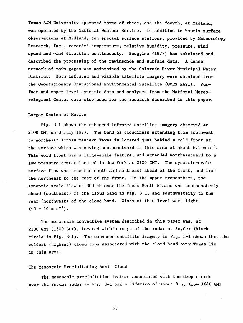
Fig. 3-1 shows the enhanced infrared satellite imagery observed at

2100 GMT on 8 July 1977. The band of cloudiness extending from southwest

to northeast across western Texas is located just behind a cold front at

the surface which was moving southeastward in this area at about 6.5 m s""1.

This cold front was a large-scale feature, and extended northeastward to a

low pressure center located in New York at 2100 GMT. The synoptic-scale

surface flow was from the south and southeast ahead of the front, and from

the northeast to the rear of the front. In the upper troposphere, the

synoptic-scale flow at 300 mb over the Texas South Plains was southeasterly

ahead (southeast) of the cloud band in Fig. 3-1, and southwesterly to the

rear (northwest) of the cloud band. Winds at this level were light

(~5 - 10 m s"1).

The mesoscale convective system described in this paper was, at

2100 GMT (1600 CDT), located within range of the radar at Snyder (black

circle in Fig. 3-1). The enhanced satellite imagery in Fig. 3-1 shows that the

coldest (highest) cloud tops associated with the cloud band over Texas lie

in this area.

The Mesoscale Precipitating Anvil Cloud

The mesoscale precipitation feature associated with the deep clouds

over the Snyder radar in Fig. 3-1 bad a lifetime of about 8 h, from 1640 GMT

37

00

Fig.3-1. GOES EAST enhanced infrared satellite photograph of the cloud pattern overthe Texas HIPLEX area at 2100 GMT on 8 July 1977. The circle outlines therange of the M-33 radar at Snyder.

on July 8 to 0100 GMT on July 9. From its first appearance as a pair of

lines of small echoes oriented from northeast to southwest at a location

about 50 km southeast of Snyder, the precipitation feature as a whole

showed little motion, although it broadened considerably towards the north

west and southeast, as well as lengthened to the northeast and southwest. Fig,

3-2 shows the low-level precipitating pattern and an RHI along the

azimuth of 3 observed by the radar at 2104 GMT, about midway through the

feature's life cycle. At this time the low level echo coverage was approxi

mately the maximum for the precipitation feature's lifetime. The vertical

cross section in Fig. 3-2a shows that an extensive anvil of precipitation

particles aloft extended to the rear of the precipitation feature at this

time. Fig. 3-2a also shows that a distinct bright band of high reflectivity

values was present in the portion of the anvil where precipitation reached

the surface. The anvil of precipitation particles aloft was quite exten

sive. The heavy dashed line in Fig. 3-2b outlines its maximum extent. This

mesoscale feature shows a strong resemblance to those observed in tropical

cloud clusters (Houze, 1975, 1977; Leary and Houze, 1978, 1979 a,b), with

its prominent bright band and horizontally oriented contours of reflectivity.

A 2100 GMT sounding at Post (see Fig. 3-2b), located near the outer

boundary of the portion of the anvil containing precipitation-sized particles,

shows further evidence of similarity with mesoscale precipitation systems

observed over the tropical ocean. The lower portion of the sounding is

shown in Fig. 3-3. In Fig. 3-4, the sounding is superposed on a collection

of soundings compiled by Zipser (1977) to depict the thermodynamic structure

of precipitating anvil clouds in the tropics, particularly those observed

during GATE. In the layer between 600 and 900 mb, the 2100 GMT sounding

at Post shows a strong similarity to tropical soundings beneath anvil clouds,

suggesting that the mesoscale subsidence due to evaporative cooling that

produces such soundings (Zipser, 1969, 1977; Brown, 1979) is also present

in this case. The surface temperature at Post is consistent with its

position outside the area where precipitation reached the surface.

The wind field in the vicinity of the mesoscale precipitation feature

at 2100 GMT also shows similarities to tropical convective systems possess

ing mesoscale subsidence beneath anvil clouds. Fig. 3-5 shows the surface

wind field at 2100 in the vicinity of the convective system. The wind flow

is strongly difluent, and the increase in wind speed downwind makes the

39

(a) DISTANCE FROM SNYDER RADAR (knfl

40

Fig3-2. RHI (a) and low-level(1 ) PPI (b) displays derivedfrom Snyder digital radardata for 2104 GMT, 8 July1977. RHI lies along lineA-A' shown in PPI. Outside countour on RHI is

boundary of weakest detectable echo, and insidecontours are for 25, 30,and 35 dBZ. Echo boundary on PPI is 25 dBZ.Range marks on PPI are at25, 40, 60, 80, 100, 120,and 130 km. The heavy dashedline on PPI outlines the

maximum horizontal extent

of precipitation particlesdetectable by radar in theanvil cloud aloft.

Fig.3-3 Temperature (solid line) and dew point (dashed line) at 2100 GMT on8 July at Post plotted in skew T - log p format. Post is located atan elevation of 771 m above sea level.

Fig3*4 The 2100 GMT Post sounding from Fig.3-3 (heavy solid line is temperature,heavy dashed line is dew point) superposed on the lower portions of Zipser's(1977, Fig. 8) collection of soundings in and beneath tropical anvilclouds associated with intense tropical convection. The soundings areplotted in skew T - los P format.

41

Fig.3-5 Surface winds at 2100GMT on 8 July 1977 superposed on the low-levelradar echo pattern ofFig.3*2b. A half-barbindicates 2.5 m a"1, anda full barb indicates5ms"1.

42

flow divergent as well. Such a wind field at the surface in the vicinity

of precipitating anvil clouds has been noted by Zipser (1969, 1977).

Aloft, fewer wind observations were available. Table 3-2 lists wind

observations at 25 mb intervals at 2100 GMT for one station (Post) at the

rear edge of the anvil cloud as well as for one station in the precipitation

area at the surface (Big Spring) and for one station in front of the

precipitation feature (Robert Lee). Their positions are shown in Fig. 3-5.

In the 350 to 250 mb (8-10 km) layer at Post, the relatively strong southerly

winds are consistent with the northerly spread of the anvil cloud to the rear

of the precipitation feature. (See Figs. 3-2a, b). Leary and Houze (1979 b)

and Houze (1977) reported similar relationships between the orientation of

the anvil and wind direction at upper levels. Comparing the strong southerly

winds at Post between 350 and 250 mb with the weaker southeasterlies and

easterlies at Big Spring and Robert Lee suggests divergence at upper levels

associated with the anvil cloud. Again, a similar relationship has been

reported for tropical cloud clusters by Houze (1977) and Lea-ry (1979).

They also observed convergence near the 700 mb level associated with anvil

clouds. This too is suggested by the soundings in Table 2. In the layer

between 750 and 500 mb (2-5 km) northerlies and easterlies at Post compare

with southeasterlies and southerlies at the two southern stations. Con

vergence in this layer would provide mass continuity to account for sub

sidence beneath the anvil.

The precipitating anvil cloud associated with a mesoscale convective

system over the Texas South Plains resembles anvil clouds observed over

the tropical ocean in its radar echo pattern, including a bright band just

below the 0 C isotherm (3.7 km), its thermodynamic structure indicative

of mesoscale subsidence below 600 mb, and its wind field that suggests

divergence near the surface, convergence in the vicinity of 700 mb, and

divergence near 250 mb. To the extent that such resemblances exist, methods

like those developed by Houze ejt. al. (1980) and Leary and Houze (1980)

to compute vertical transports of mass and heat in tropical cloud clusters

using digitized radar data may also be applicable to intense convective

systems in middle latitudes.

43

Table 3-2

WIND DIRECTION (DEGREES) AND SPEED (M S"1) AT 2100 GMT

LEVEL (MB) POST BIG SPRING

(BGS)ROBERT LEE

(RBL)

850 084/6.6 054/7.4 091/3.8

825 048/3.3 053/6.0 138/6.3

800 347/3.0 035/4.6 149/6.6

775 347/1.9 357/0.8 143/7.9

750 025/2.4 200/2.0 147/7.3

725 045/2.1 168/1.6 145/5.8

700 073/1.6 158/1.0 135/5.5

675 098/1.6 210/0.9 135/5.0

650 006/1.1 155/0.7 118/4.1

625 315/3.2 162/2.0 096/3.8

600 317/3.2 187/2.7 111/4.0

575 334/3.0 176/1.8 134/4.7

550 329/3.1 095/1.8 123/4.4

525 321/3.5 092/1.8 128/3.1

500 345/2.8 163/1.5 137/4.6

475 041/1.5 161/2.6 130/5.3

450 120/3.1 176/8.1 114/4.4

425 139/3.1 163/15.2 174/3.3

400 144/3.4 149/9.9 175/6.7

375 208/1.7 148/10.5 166/5.8

350 212/6.7 156/11.0 147/4.5

325 169/13.9 159/9.6 151/6.4

300 172/14.8 158/7.3 137/8.3

275 179/12.3 169/1.4 127/7.2

250 180/11.5 154/2.4 082/1.3

225 188/8.6 074/1.6 029/2.9

200 206/8.6 077/0.6 078/4.4

44

Rainfall Network Data Processing and Analysis

The purpose of the rainfall analysis is two-fold; first to investigate

the use of surface rainfall and rainfall-calibrated radar data as response

variables in seeding evaluation, and second, to derive rainfall input to

hydrologic models. In either case an effort is being made to define

"natural variability" as it applies to storms in the Texas HIPLEX region.

Analysis of 1977 and 1978 field-season data has been completed. Iso-

hyetal maps of surface rainfall patterns with 15-minute temporal resolution

have been produced for each storm in which significant rainfall was collected

by the raingage network. Rainfall intensity and duration, storm size and

velocity and total integrated rainfall have been studied as a function of

synoptic and syb-synoptic weather patterns. A technical report on Texas

HIPLEX rainfall will be published at the completion of the 1979 data analysis.

Total water volume has been computed for selected rainfall periods by

first constructing a network of triangles defined by the gage locations,

computing the average rainfall over each triangle and summing over the

entire network. The results of this analysis are shown in Tables 3-3 and

3-4 for 1977 and 1978 respectively. Note that total volume is expressed

in both acre-feet and cubic meters.

Additional storm data is provided in Tables 3-5 and 3-6. In these

tables, the storm period refers to the total time that rainfall was ob

served in the network and the storm movement reflects the average move

ment of the entire storm during the period. The individual storm units

represent one or more cells which produced identifiable rainfall patterns

at the surface. Maximum storm area is the largest area enclosed by the

0.1 inch isohyet.

For the storms analyzed, rainfall periods varied from 3 hours on

21 June 1977 to 6h hours on 3 July 1978. This extended period of rainfall

was associated with strong surface heating in a moist unstable air mass

and resulted in the development of a large number of storm units (convec

tive cells). Shorter periods were related to the passage of short waves

at upper levels or.air mass discontinuities at the surface.

45

Date

21 June

21 June

22 June

22 June

Table 3-3 1977 Precipitation

Rainfall Volume

Time Period (CDT) Acre-Feet 106 m3

0000-0015 7614 9.391

0015-0030 7785 9.602

0030-0045 7720 9.522

0045-0100 8634 10.649

0100-0115 8968 11.061

0115-0130 8373 10.327

0130-0145 8235 10.157

0145-0200 5528 6.818

0200-0215 5997 7.397

0215-0230 5686 7.013

0230-0245 2684 3.311

0245-0300 1391 1.716

2245-2300 2291 2.826

2300-2315 2673 3.297

2315-2330 2158 2.662

2330-2345 2004 2.472

2345-0000 1767 2.179

0000-0015 758 0.935

0015-0030 580 0.715

0030-0045 476 0.587

0045-0100 434 0.535

1300-1315 670 0.826

1315-1330 908 1.120

1330-1345 1746 2.154

1345-1400 2550 3.145

1400-1415 4122 5.084

1415-1430 2311 2.850

1430-1445 3652 4.504

1445-1500 2381 2.937

1500-1515 1359 1.676

1515-1530

1530-1545

1545-1600 2844 3.508

1600-1615 5262 6.490

1615-1630 2831 3.492

1630-1645 2387 2.944

1645-1700 4100 5.057

1700-1715 3631 4.479

1715-1730 2633 3.248

1730-1745 3065 3.780

46

Date

23 June

23 June

8 July

Table 3-3 (cont.)

Rainfall Volume

Time Period (CDT) Acre-Feet 106 m3

0415-0430 951 1.173

0430-0445 565 0.697

0445-0500 1031 1.272

0500-0515 835 1.030

0515-0530 592 0.730

0530-0545 315 0.389

0545-0600 441 0.544

1500-1515 3078 3.796

1515-1530 2462 3.037

1530-1545 2549 3.144

1545-1600 2391 2.949

1600-1615 1299 1.602

1615-1630 647 0.798

1630-1645 1606 1.981

1645-1700 3395 4.187

1700-1715 2707 3.339

1715-1730 1712 2.112

1730-1745 1250 1.542

1745-1800 2233 2.754

1800-1815 1671 2.061

1815-1830 1374 1.695

1330-1345 4046 4.990

1345-1400 5004 6.172

1400-1415 4574 5.642

1415-1430 5727 7.064

1430-1445 8875 10.947

1445-1500 9268 11.431

1500-1515 5871 7.241

1515-1530 6198 7.645

1530-1545 4046 4.990

1545-1600 1919 2.367

1600-1615 1184 1.460

1615-1630 926 1.142

1630-1645 1033 1.274

1645-1700 1009 1,245

47

00

I—»l—»l—*l—•!—«l—»h-*l-Jl—'vO^OVOVOOOOOOOCOsj*>WHOJMJHOJSUiOCnOOiOLnOLn

IIIIIIIIIl>0I—•I—»t—•I—»I—»I—•I—»I—•OVDVOVOVOOOOOOOOOO-0u>h-»O-P»WMOOUiOV-nOUiOCnO

c

OONUi0000004>-OU)J^N3tO

vOUih-'UiO^JtOONVOLnW-P*NONWUOONsJsJOWC^^

W*»Ui0J->0>4>-tOtOC0UJI-»

00CnUiUi0>OtOUiv0OV0LnHOONH\OOM*»*-MVOW

OMOOIo

Ui

I—»I—»I—•I—»tolototo4>oh-«o•>

imoUit-»iiItoMMh-»4StototoUiCOH-«O

OUiO

M»-»M\->OO->OUiII

OOMOLnI

I-*OOt-»WUiO

Ci

OOOOOOv©v©vovo0000

CJt-»O•!>•U>OCnOLnOIIIIIOOOOOVOVOVOVO00U)UHO*»OnOv/iO<-n

HPHHPNUWJSUivnNNJ*>vl00HOiUiNUiHH>J00(jN|v5HC»^HLnsjvOUiWOOUi.MoJ>>^sJONslH,»JN3N300vlUiOOOOH^NOO^VD^^HONUO^tOON

oooi-»MHHMW->U<OM3NtOHOO

toLnvOO->VOVOLnOOO>OOOAvOV04S*ONOCfNtOHOONj^OUiHWVO^OOUivOVOWOOHJS'lv)sj^^OOJSOslMvjjsjsUivOUiJSOvO^vO

Ui

MtOIOHHHHHHHHHHHOOOVO^VOVOOOOOOOWnIsJsIWHO*-U)HO*«WHO^WHOv^OUiOUiOLnOLnOV-nOCnIIIIIIIIIIIIIItOtOtOtOM|-'l-,H*hJh-'H-»h-,l-'H»OOOOVOVOVOVOOonOOGOMM

CnOV-nOLnOLnOv^OUiO«-nOLn

OO^JOOOOOOONOOVOJSLOOiWH*0\00\OOUivOVOW^M^H'^ff|VO00Ui00V0V0vJUi*»VOO4MflslHONiLnOOOvOOOslWOOW^OOMOOUi

OH^(»OM-'MOHUlW^*>N

OOOvOvlOHOOOO^OJO^OO^J^W4SLn|-i4SOO-IS*tOOOLnOVOUiO\UiNj(jivOUiffi*400MOHUilnMWO

rt

I

O

a

>

n>i

*Jn>n>rt

MO

6-

U>I

VO

00

n

OH«

vo

00oooo

LnOUiIIIH*K»MVO0000O-t>LOOUiO

H»MH*00"»J*vl

O4SOLnIIMM0000H"OLnO

LOOIH»

Ln

to

LO

<-*C

MMMMh-'h-'l-'t-'l-'H-1

HO*»WHO^U)HOUiOUiOLnOUiOUiO

IIIIIIIIIIl-J^-»^-,l-,^-,^-*l-,^-Jl-J^-,

WHO^WHO^WHOUiOUiOUiOUiOLn

H'l-'HLO-e-UiONUitOIOfOtOUiUi«vjv04>**00OtOL0H»0N^JLnL000L0h-'L0LnOL00>V000hJUitOL0L000OUivJVOODWN^slOOsJWtOslHsiai

OOOHHHMW^^MONWWNU

O^OivOHsJNJW00(Oln'Ji*OWHvOJS0>L0l-»00L0ONOtO00Ln00L0^JtO4^ONOOOtOtOHONlOOvOOOVO-I^ONtOj^H

0000^J-J-«JI-1O-P*U>UiOUiIII

OI

000000WHOOUio

LOOUi

toto

C

hJMH-,t-'»-'hJH-'l-,l-,l-»l-'ONONONONUiUlUlUlJ^**^•l^»L0l-»O4^*L0l-,O4^•L0l-,LnOUiOUiOUiOUiOUiIIIIIIIIIII

»-»H,l-,HJl-»l-»l-*l-*l-«MM-«JO^O^O^O^U^L^L^L^.J>•£,•OMoHO*>WHO>UOUiOUiOUiOUiOUiO

LOLOtotoLOLOMHK3HMOOOK3MHOHHONOOMM-1L0OI-,00L04NV0UiUlUlUi,vJUlVOV0tO0>OiNjUltOtOOMjlW^HOO^WNlMslON

OOOOHU^NNUUHOl-'OOO

HN3HWOvlO^ONNJO)*.OOHONUiN)0>Ui-P^45»tOUiO>^JUiONV04>-OOOtOO00UitO00O\NjJ^kONl0Jln00UiO\v|s4ln

u>

oOPrt

tototototototototototorototototoWWWUNNNNHHHHOOOO**WHO4MjJHO*«0JHO^WHOUiOUiOLnOUiOLnOUiOLnOUiO

IIIIIIIIIIIIIIIIotototototototototototorotototoOLOLOLOLOtOtOtOtOMHJMH,000

OLnOUiOUiOUiOUiOUiOUiOUi

HJ-»H-»MH*HN3N3HHW-«JLnL0V0IOtOtOUlOtOV0L0L00>00OOw^VO^HVOVOsJMMNJHMOOH4SOi4N00V0slW00WOOiUi00v4(O

OOOHh'HHHHHHMNJNMW

OOOJSIOUlUlONVOLOUll-JOOOOOtO^JOMnKJN^OOOMrfslWO^UiNjNJOUiv00N0>JS»4^OUiOOUi00LnOVOL0

pa

I

o

o

>oHn>i

n>a>rt

O

LOI

4>»

oo

rt

Table 3-5 1977 Storm Data

DATE PERIOD MOVEMENT INDIVIDUAL STORM UNITS

(hrs) (km/hr) (deg) UnitLifetime

(hrs)Max. Area

(km2)Max. Intensity

(in/hr)

21 June 77 3.00

22 June 77 4.25

23 June 77 3.50

8 July 77 3.50

32

24

10

30

320

300

110

165

A 2.75 2680 2.2

B 0.50 375 0.8

C 0.25 1219 1.4

D 0.75 760 1.2

E 1.50 700 1.9

F 0.75 405 1.7

G 0.50 250 0.6

A 2.50 920 1.0

B 0.75 195 2.1

C 0.50 800 2.1

D 0.75 276 0.5

E 1.75 560 1.6

F 2.00 1140 2.2

G 1.00 1554 1.5

A 2.00 810 3.0

B 2.00 624 2.6

A 3.00 966 3.4

B 0.75 136 1.9

C 2.25 760 2.3

D 0.75 380 1.5

E 0.50 440 2.5

F 0.75 252 1.2

G 0.50 437 0.2

50

Table 3-6 1978 Storm Data

DATE PERIOD MOVEMENT INDIVIDUAL STORM UNITS

(hrs) (km/hr) (deg) UnitLifetime

(hrs)Max. Area

(km2)Max. Intensity

(in/hr)

5 June 78 3.75 16

3 July 78 6.50 32

22 July 78 4.25 14

280

290

290

A 2.25 1290 5.6

B 0.25 260 1.2

C 0.75 500 1.7

D 2.25 1760 3.6

E 0.75 805 0.5

A 1.50 504 1.1

B 0.50 320 0.6

C 0.50 208 0.6

D 2.50 300 1.7

E 0.50 476 0.4

F 1.50 855 1.6

G 1.50 308 1.3

H 1.25 1880 1.5

I 0.50 264 1.3

J 1.00 340 1.2

K 2.00 440 1.4

L 1.25 168 0.9

M 1.50 858 0.4

A 0.50 144 0.6

B 1.00 276 0.2

C 0.75 340 0.4

D 0.75 462 0.6

E 1.25 312 1.1

F 1.75 532 2.2

G 1.50 187 1.7

H 1.75 576 2.0

51

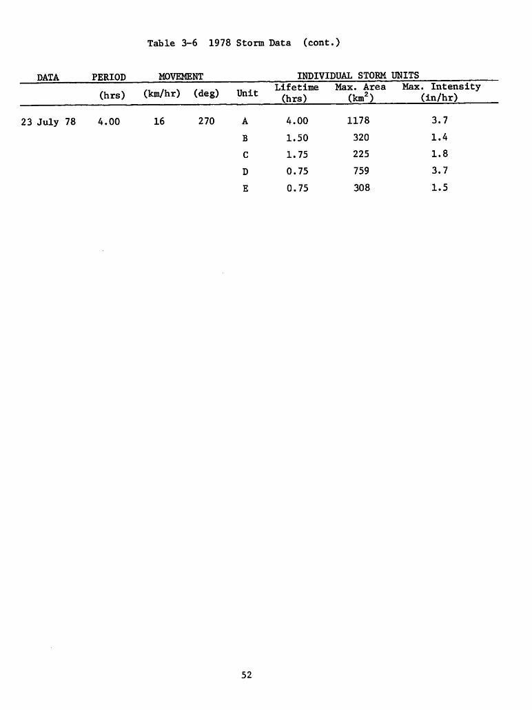
Table 3-6 1978 Storm Data (cont.)

DATA PERIOD MOVEMENT INDIVJ[DUAL STORM IJNITS

(hrs) (km/hr) (deg) UnitLifetime

(hrs)Max. Area

(km2)Max. Intensity

(in/hr)

23 July 78 4.00 16 270 A 4.00 1178 3.7

B 1.50 320 1.4

C 1.75 225 1.8

D 0.75 759 3.7

E 0.75 308 1.5

52

Note that rainfall intensities, based on 15-minute data resolution,

ranged from less than 0.5 inches per hour to more than 5.5 inches per

hour in the heaviest storm. A storm classification system based upon

rainfall intensity, storm duration, rainfall volume, time between events

and meso-synoptic weather type is being developed as a first step in

generating long periods of precipitation for input to hydrological models.

Rainfall data collected during the 1979 field season have been pro

cessed in a manner acceptable to the Water and Power Resources Service and

forwarded to Denver for archival purposes.

Task 4. Radar Data Collection for the 1979 Field Experiment

On each day during the 1979 HIPLEX season when convective echoes were

present, the SKYWATER radar was used to record digital radar. In addition,

16mm movies of the color television display were obtained to supplement

the digital data collected on magnetic tape.

Table 4-1 lists the four scanning modes in which the digital radar

data were recorded. The two aircraft modes were employed when HIPLEX

cloud treatment missions were in progress. If the clouds to be treated

were more than 50 km from the radar, the Aircraft Far Out mode was

employed, while if the clouds to be treated were located within 50 km

of the radar, data were recorded using the Aircraft Close In mode.

When aircraft flew near cloud base to collect data for comparing radar

reflectivity to rainfall rate, the Z/R mode was used. Data was re

corded in the Monitoring mode when the HIPLEX aircraft were not engaged

in a mission. Table 4-2 lists the times for which digital radar data

was recorded in each of the four scanning modes. Table 4-3 lists the

times for which 16 mm color photographs were obtained.

During aircraft operations, radar observations were made available

whenever possible for guidance in the deployment of aircraft for cloud

monitoring and treatment. Video tape recordings of the color television

display, which showed the positions of HIPLEX aircraft made it possible

to discuss aircraft operations during debriefings with reference to

53

PRF

RANCE

INTERVAL

RANGE

DELAY

A-SCAN

Samples

Elevation

B-SCAN

Table 4-1

SKYWATER RADAR

TEXAS HIPLEX SCANNING MODES

1979

Monitoring(MON)

Z/R(ZR)

Aircraft

Far Out

(ACF)

Aircraft

Close In

(ACC)

414 414 414 414

1 Km 0.5 Km 0.5 Km 0.5 Km

10 Km

16

,o

10 Km

16

0.5'

10 Km

16

,o

10 Km

16

.o

Samples 16 32 8 8

Start 2° 1° 2° 2°

Stop 12° 3° 12° 20°

Steps 1° 0.5° 0.5° 1°

timi:10 Min 5 Min 5 Min 5 Min

INTERVAL

54

Table 4-2

INVENTORY OF DIGITAL RADAR DATA

Original Start End

Tape A-file Time Time

Calendar Date Label Name Mode (GMT) (GMT)

20 May 1979 / T9140 A// AT0140V ACC 212641 220145

itT9140 B#

it

ACC 220622 224530

iiT9140 C#

it

ACC 225256 2330

ii

T9140 D#ti

ACC 233318 000743

M

T9141 A// AT9141B ACC 010021 011135

27 May 1979* T9147 A AT9147P MON 154420 172820

uT9147 B

itMON 173417 192834

itT9147 C

iiMON 193414 212910

iiT9147 D

iiMOM 213413 232842

,: T9147 Eii

MOM 233415 011000

iiT9148 A

i:ACC 011128 014043

itT9148 B

itMON 014447 034930

H

T9148 Cti

MON 035510 042410

28 May 1979* T9148 D AT9148T ACF 191732 194942

i.T9148 E

it

ACF 195333 202305

•? T9148 Fi:

MON 202540 220940

31 May 1979 T9151 A AT9151S MON 181855 185436

i:

T9151 Bit

ACC 185740 193152

iiT9151 C

it

ACC 193248 200158

it

T9151 Dii

ACC 200315 203226

i.

T9151 i;it

MON 203636 223056

iiT9151 F

iiMON 223635 003056

i. T9152 Aii

MON 003217 021639

i: T9152 Bii

MON 021745 031341

i: Indicates 16 mm movieI of the color television display not availabe

for the time period of this tape* Indicates a mesoscale day/ Indicates a rapid scan day

55

Original Start End

Tape A-file Time Time

Calendar Date Label Name Mode (GMT) (GMT)

1 June 1979* T9152 C AT9152P MON 151902 170712

it T9152 Dtt

MON 171005 183322

it T9152 E AT9152S MON 185558 204019

tt T9152 Fti

MON 204610 224019

ti T9152 Git

MON 224558 003503

t?T9153 A

itMON 003717 020131

2 June 1979 T9153 B AT91530 MON 140740 154201

nT9153 C

tiMON 4 154740 173202

it

T9153 Dti

MON 173740 192201

t:

T9153 E1!

MON 192740 212202

4 June 1979* T9155 A AT9155R MON 172117 175538

it

T9155 Bit

ACC 175739 182649

ti

T9155 Cn

ACC 182753 190202

ti

T9155 Dii

ACC 190309 193643

nT9155 E

ti

ACC 193742 201151

ir

T9155 Fti

ACC 201257 204206

tiT9155 G

1!MON 204427 213849

tt

T9155 IIII

ACC 214126 220221

it

T9155 Ji:

ACC 220520 223929

i:T9155 K

it

ACC 224030 230944

t;T9155 L

itMOM 231225 005654

i;

T9156 Aii

MON 010000 024300

* Indicates a mesoscale day

56

Original Start End

Tape A-file Time Time

Calendar Date Label Name Mode (GMT) (GMT)

5 June 1979* / T9156 B AT9156T MON 192900 201420

iiT9156 C ti

ACC 201604 205013

ttT9156 D it

ACC 205116 . 210524

ttT9156 E

itMON 210659 222512

ttT9156 F

•tACC 222512 224921

iiT9156 G it

ACF 225107 231540

iiT9156 H

t:

MON 231743 010205

7 June 1979 / T9158 A AT9158U MON 205300 223719

8 June 1979* / T9159 A AT91590 MON 141124 155545

ii

T9159 Bti

MON 160124 174545

i;T9159 C

tiMON 175124 192555

ii

T9159 Di*

MON 193728 212150

IiT9159 E

iiMON 212535 230955

it

T9159 Fn

MON 231418 005839

ii

T9160 Aii

MON 005957 014500

nT9160 B

iiMON 015204 025634

9 June 1979* T9160 C AT91600 MON 145115 163530

itT9160 D

itMON 164109 181830

21 June 1979* T9172 A/< AT9172U MON 203400 222821

ii T9172 B H i;MON 223400 002822

23 June 1979 T9175 A AT9175B MON 013218 022640

1!

T9175 B AT9175E MON 043806 051236

* Indicates a mesoscale day// Indicates 16 mm movie of the color television display not available

for the time period of this tape/ Indicates a rapid scan day

57

Original Start End

Tape A-file Time Time

Calendar Date Label Name Mode (GMT) (GMT)

24 June 1979* T9175 C AT9175T MON 195717 203140

it T9175 Dit

MON 203801 222223

t:T9175 E

ti

MON 222511 000934

tt T9176 Ait

MON 001053 002600

25 June 1979 T9176 B AT9176Q MON 163845 182306

ttT9176 C MON 182522 192501

it

T9176 D ACC 193823 200743

tiT9176 E ACC '201309 204219

t:T9176 F ACC 204646 211555

iiT9176 G ACC 212155 215105

itT9176 H MON 215549 234009

itT9176 J MON 234212 012635

26 June 1979 T9177 A AT91770 MON 145150 163609

" T9177 Ii MON 164200 181314

tiT9177 C MON 182148 195130

itT9177 D ACF 195331 201804

tiT9177 E MON 202120 215735

itT9177 F MON 220121 223551

2 July 1979* T9184 A AT9184D MON 032150 050619

3 July 1979* T9184 B AT9184S MON 182200 201631

itT9184 C

i*MON 202356 220826

iiT9184 D

tiMON 221341 000610

iiT9185 A

HMON 001111 002820

itT9185 B

iiACC 003424 010333

tr

T9185 Ci*

ACC 010852 013801

i:T9185 D

ii

ACC 014235 021145

i;T9185 E

•iMON 021810 024234

Indicates a mesoscale day

58

Calendar Date

OriginalTape

Label

A-file

Name Mode

Start

Time

(GMT)

End

Time

(GMT)

4 July 1979* T9185 F AT9185S MON 184337 202100

it T9185 G " MON 202832 221812

tt T9185 Hti

MON 222959 235800

5 July 1979* T9186 A AT9160O MON 143501 161932

it T9186 Bti

ACC 165119 172029

tiT9186 C

itACC 172509 175420

ti T9186 D AT9186S ACC 185314 192223

ii T9186 Eit

ACC 193029 195938

IT T9186 Fit

ACC 200437 203347

II T9186 Gii

ACC 203901 210811

Ii T9186 HI!

ACC 211316 214226

II T9186 Jtr

ACC 214815 222156

t: T9186 Ki*

MON 223334 235910

ti T9187 A AT9187C MON 020348 025818

6 July 1979* T9187 B AT9187S MON 182055 194031

i: T9187 C AT9187U MON 203428 221850

it T9187 Dti

MON 222616 223240

tt T9187 Ei; MON 225321 003742

i. T9188 A AT9188B MON 014527 022200

7 July 1979* T9188 B AT9180O MON 145405 162827

ii T9188 Ci;

MON 163410 181832

it T9188 Dii

MON 182416 190837

it T9188 E AT9188W MON 225421 232850

M T9188 Fit

ZR 233856 010242

* Indicates a mesoscale day

59

Calendar Date

OriginalTape

Label

A-file

Name Mode

Start

Time

(GMT)

End

Time

(GMT)

8 July 1979 T9189 A# AT9189U MON 203921 205340

T9189 B#1!

ACC 205929 212842

T9189 C#1?

ACC 213325 220235

T9189 D AT9189X ZR 232640 003222

T9190 Ait

MON 003700 022300

T9190 Btt

MON 023009 030430

9 July .1979 T9190 C AT9190P MON - 153938 172800

itT9190 D AT9190V ZR 210314 211154

i:T9190 E

itACC 211525 213550

it T9190 FIT

ACC 214008 214931

tiT9190 G

11ZR 215222 222107

i;T9190 H

IIMON 222428 000852

t?T9191 A

IIMON 002035 020456

itT9191 B

IIMON 021050 034512

12 July 1979 T9193 A AT9193Q MON 163424 182846

itT9193 B

itMON 183341 201802

14 July 1979* T9195 A AT9195P MON 152826 172247

itT9195 B

itMON 172842 185310

// Indicates 16 mm movie of the color television display not availablefor the time period of this tape

* Indicates a mesoscale dav

60

Original Start End

Tape A-file Time Time

Calendar Date Label Name Mode (GMT) (GMT)

15 July 1979 T9196 A AT9196U MON 200853 210322

T9196 B ACF 210903 213333

T9196 C ACF 213753 220225

T9196 D MON 220707 235129

T9196 E MON 235628 014048

T9197 A MON 014527 031948

T9197 B MON 032429 035851

16 July 1979* T9197 C AT9197S MON 182810 202231

11 T9197 Dti

MON 202842 222305

it T9197 Et:

MON 223100 233528

t: T9197 Fti

ACF 234719 001152

ii T9198 Ait

MON 002309 005500

17 July 1979*/ T9198 B AT91980 MON 144803 163223

ti T9198 Cit

MON 163731 182152

t: T9198 Cti

MON 182813 195233

ii T9198 Ett

ZR 200140 205019

ii T9198 Fii

ACC 205327 210800

ii T9198 Git

ACC 211505 214406

tt T9198 IItt

ACC 214850 221758

ii T9198 Jit

MON 222233 000654

itT9199 A

tiMON 001148 015610

it T9199 B » MON 020139 025610

* Indicates a mesoscale day

/ Indicates a rapid scan day

61

Original Start End

Tape A-file Time Time

CajLdendcir Date Label Name Mode (GMT) (GMT)

18 July 1979*/ T9199 C AT91990 MON 144837 164320

itT9199 D

itMON 165431 184853

tiT9199 E

iiMON 185500 204922

itT9199 F AT9199V MON 212356 231816

tiT9199 G

ttMON 232337 011758

1!T9200 A

tiMON 012544 030005

19 July 1979 T9200 B AT9200O MON 143359 161846

i:T9200 C

iiMON 162515 181935

iiT9200 D

ttMON 182752 202213

tiT9200 E AT9200U MON 205414 224836

itT9200 F

ttMON 225426 004847

20 July 1979 T9201 A AT9201O MON 145008 164437

tiT9201 B

i«MON 165008 17.1510

* Indicates a mesoscale day/ Indicates a rapid scan day

62

Table 4-3

INVENTORY OF 16MM MOVIE FILM

Start End

Reel Julian Time Time Calendar

Number Day (GMT) (GMT) Day

1 146 1422 1433 26 May

1! ti 1912 2012ii

It 147 1534 2400 27 May

II 148 0000 0420ii

II it 1916 2209 28 May

2 151 1840 2400 31 May

it 152 0000 0314it

.i: ii1419 2400 1 June

ii 153 0000 0201ti

it t: 1405 2122 2 June

1!155 1721 2400 4 June

It156 0000 0243

l:

i: it1855 2305 5 June

3 158 2124 2237 7 June

it 159 1350 2400 8 June

i' 160 0000 0257it

it ti 1350 1505 9 June

ti tt 1522 1816ti

4 175 0132 0233 23 June

tt 0438 0512i>

ii 1947 2400 24 June

176 0000 0034ii

it 1639 2400 25 June

177 0000 0127ti

ii 1444 2246 26 June

63

Start End

Reel Julian Time Time Calendar

Number Day (GMT) (GMT) Day

5 183 2137 2137 1 July

tt 184 0314 0511 2 July

ti tt 1806 2400 3 July

it 185 0000 0251ii

it tt 1844 2324 4 July

it 186 1435 2318 5 July

6 186 2333 2400 5 July

ti 187 0204 0258it

1! t; 1820 2400 6 July

It 188 0000 0219ii

II ti 1453 1909 7 July

II ii 2254 2400ii

II189 0000 0037

it

II H 2322 2400 8 July

II190 0000 0304

it

11 t: 1539 1722 9 July

II 1!2103 2400

it

It191 0000 0025

ti

i; ii 0114 0345ii

i.193 1634 2018 12 July

ti 195 1524 1901 14 July

7 196 2012 2400 15 July

it197 0000 0359

it

it ii 1828 0000 16 July

it 198 0023 0102it

i: it 1447 0000 17 July

ti199 0000 0256

it

i? i: 1449 2400 18 July

it200 0000 0300

it

ii ii 1434 2026 19 July

64

Start End

Reel Julian Time Time Calendar

Number Day (GMT) (GMT) Day

8 200 2054 2400 19 July

tt201 0000 0048 i n

t: t!1450 1715 20 July

65

Table 4-4

INVENTORY OF RADAR VIDEO TAPES

SUMMER 1979

Start End

Calendar Tape Julian Time Time

Day Number Day (GMT) (CMT)

May 27 1 148 005509 015732

May 31 2 152 144559 145601

June 4 3 155 153440 153536

June 4 3 155 152527 153145

May 28 3 148 153510 154045

June 4 4 155 193136 203344

June 5 5 156 222150 232300

June 8 6 159 215827 230128

June 8 7 159-60 230827 001100

June 25 8 176 144351 150944

June 25 9 176 195634 205905

June 25 10 176 210245 220531

June 26 11 177 ' 200201 201400

July 19 12 200 144140 144455

July 2 12 184 032715 042623

July 3 13 184 214500 224811

July 3 14 185 003246 013526

July 3 15 185 014546 024600

July 4 16 185 210242 220720

July 5 17 186 165216 175505

July 5 18 186 201719 211947

July 7 19 188-89 234146 003830

July Q 20 190 212000 222255

July 15 21 196 211655 221830

July 15 22 197 003116 012449

July 15 22 197 022650 023547

July 16 23 197-98 225800 004405

July 17 24 198 204849 214940

July 17 25 160 145637 150540

July 17 25 198 145610 150600

66

Start End

Calendar Tape Julian Time Time

Day Number Day (GMT) (GMT)

July 17 25 199 000030 004345

July 18 26 199--200 231825 002126

67

changing echo patterns. Table 4-4 lists the times for which video tapes

made during the field project were saved for later analysis.

Weekly calibration tapes were mailed to the Bureau. Digital data

tapes were all mailed to the University of North Dakota where they were

edited with little or no delay after they were received. Processing

through the University of North Dakota's RADPROC programs has also

been completed on all 172 tapes.

Task 5. Support to the Field Program

During the 1979 Texas HIPLEX field program, a Laserfax was supplied

by the Water and Power Resources Service to provide around-the-clock real-time

support for the field operations. Texas Tech was responsible for the

collection of visible and infrared imagery and their interpretation

regarding the formation, location and degree of development of convec

tive clouds. The information was provided in support of forecasting for

operational decisions, declaration of mesoscale operational days and

deployment of aircraft. The availability of both the specialized equip

ment and a meteorologist trained in the interpretation of satellite

imagery proved to be a real asset to the program. A particularly

valuable contribution proved to be to the calling of a mesoscale opera

tional day. The 30-minute time resolution GOES imagery provided the only

current information, in addition to surface observations, available

before the decision on a mesoscale day was required. Besides providing

input to forecast decisions, the GOES imagery was incorporated into both

the daily weather briefings and the aircraft mission debriefings. The

perspective of prevailing synoptic processes provided through this effort

was recognized as highly beneficial to the field program. In addition,

an opaque projector was generously loaned to us for the duration of the

project by Howard College. This permitted the satellite imagery to be

more effectively displayed and discussed during the daily weather briefings.

68

REFERENCES

Brown, J.M., 1979: Mesoscale unsaturated downdrafts driven by rainfallevaporation: A numerical study. J_. Atmos. Sci., _36, 313-338.

Houze, R.A., Jr., 1975: Squall lines observed in the vicinity of theResearcher during Phase III of GATE. Preprints 16th Radar Meteorology Conf., Houston, Amer. Meteor. Soc., 206-209.

, 1977: Structure and dynamics of a tropical squall-line system. Mon. Wea. Rev., 105, 1540-1567.

, C.-P. Cheng, C.A. Leary, and J.F. Gamache, 1980: Cloudmass and heat fluxes over tropical oceans: Diagnosis from radarand synoptic data. J_. Atmos. Sci., in press.

Leary, C.A., 1979: Behavior of the wind field in the vicinity of a cloudcluster in the Intertropical Convergence Zone. J_. Atmos. Sci. , 36631-639.

, and R.A. Houze, Jr., 1978: Observations of horizontallyuniform precipitation and radar bright bands in the tropics. Preprints 18th Conf. on Radar Meteorology, Atlanta, Amer. Meteor. Soc,1-8.

, and , 1979a: Melting and evaporation of hydro-meteors in precipitation from the anvil clouds of deep tropical convection. J_. Atmos. JSci. , ^6, 669-679.

, and , 1979b: The structure and evolution ofconvection in a tropical convection. J_. Atmos. Sci., 36^ 437-457.

, and , 1980: Cloud mass and heat fluxes overtropical oceans: The role of mesoscale motions in intense convectivesystems. J_. Atmos. Sci. , in press.

0£.ura, Y. , and M.-T. Liou, 1979: The structure of a mid-latitude squallline: A case study. Submitted to J_. Atmos. Sci.

Sanders, F., and R.J. Paine, 1975: The structure and thermodynamics ofan intense mesoscale convective storm in Oklahoma. J_. Atmos. Sci.,32, 1563-1579.

, and K.A. Emanuel, 1977: The momentum budget and temporalevolution of a iresoscale convective system. J_. Atmos. Sci. , 34,322-330.

Scoggins, J.R., 1977: Texas HIPLEX Mesoscale Experiment - Summer 1977Data Tabulations. Final Report, TWDB Contract No. 14-70030. Availablefrom Texas Department of Water Resources, Austin, Texas.

69

Zipser, E.J., 1969: The role of organized unsaturated convective down-drafts in the structure and rapid decay of an equatorial disturbance.J_. Appl. Meteor., S, 799-814.

, 1977: Mesoscale and convective scale downdrafts as distinct

components of squall-line circulation. Mon. Wea. Rev., 105, 1568-1589

Zwack, P., and C. Anderson, 1970: 25 July 1969: Showers and continuousprecipitation. Preprints 14th Radar Meteorology Conf., Tucson,Amer. Meteor. Soc., 335-338.

70