“… no exceptional brain power is needed to construct a new science or expand on an existing

one. What is needed is just the courage to face inconsistencies and to avoid running away

from them just because ‘that’s the way it was always done’.” (Eliyahu M. Goldratt. Introduction

to the Second Edition of “The Goal”)

From the Flawed “Theory of Constraints”

to Hierarchically Balancing Criticalities (HBC)

Dan Trietsch

May 2004

Abstract:

The so-called “Theory of Constraints” (henceforth “TOC”) as articulated and

explained in Goldratt’s books, is neither a theory nor a correct methodology.

Nonetheless, in practice, it often leads to major successes. I interpret the term

Management by Constraints (MBC) as the correct aspects of “TOC,” and argue that

successful MBC applications never follow “TOC” with complete faithfulness. “TOC”

involves an internal inconsistency that must be faced courageously: To make drum-

buffer-rope (DBR) work, Goldratt forbids balance, and yet Step 4 promotes balance.

MBC implicitly rejects DBR and allows balance. We should go further and seek

economic balance. The next step is to pursue balanced economic growth in

hierarchical systems. In effect, the result is a combination of MBC and of policy

deployment aimed to improve both.

1. Introduction and Mission Statement

Charismatic persons occasionally influence the course of scientific discovery. For

instance, consider Dr. Franz Anton Mesmer (1734-1815), whose very name now “suggests”

charisma (http://www.whonamedit.com/doctor.cfm/313.html). To say that he had been

influential is a major understatement. Where would we be without hypnosis? Where would

hypnosis be without Mesmer? Although Mesmer had not invented hypnosis, he “put it on the

map.” But it took a long time for the establishment to accept that “mesmerism” can be useful

in spite of the fact that Mesmer’s theories look preposterous (unless one is under mesmeric

trance). Historically, perhaps for this reason, the term “mesmerism” has been discarded

before hypnosis was fully accepted.

The so-called “Theory” of Constraints (“TOC”) is also associated with a mesmerizing

promoter, Eliyahu M. Goldratt. Except for charisma and influence, any similarity between

Goldratt and Mesmer is purely coincidental. Yet, perhaps because charismatic and prominent

leaders tend to attract both admiration and opposition, Mesmer had his share of followers and

detractors and so does Goldratt. Unlike Mesmer’s detractors, however, most of Goldratt’s

chose to officially ignore him. Armed with more than 20 years worth of 20/20 hindsight, in

my opinion this “strategy” has failed.1 One result is that not enough had been done to show

formally that the theoretical aspects involved in Goldratt’s work are flawed, specifically

where they differ from JIT. Elsewhere (Trietsch 2003; henceforth T03), I discuss several such

points—one of which is central to this paper and will be repeated later. An example of the

type of damage that was caused by the critics’ silence is that academics often teach inferior

methods such as Drum-Buffer-Rope (DBR) although even Goldratt himself stopped using it

for scheduling. Furthermore, not enough had been done to move forward. I believe that

1 With apologies, (i) I will often use the first person singular; (ii) I will reference my previous work more than is usually acceptable in polite society. The paper is based on my personal take of the “Goldratt phenomenon” and my previous writings, so it would be difficult to avoid these transgressions.

1

progress had been limited due to a reason similar to the reluctance of modern professionals to

use the term “mesmerism.” If so, we need new terms as well as a clear distinction between

doing research in this field and accepting Goldratt as an academic leader. On the one hand, he

is an insightful and influential OM teacher, who probably promoted OM more than we could

achieve without him. On the other hand, his teaching requires major and minor corrections

and should not be trusted academically.2

I will adopt a term coined by Ronen, Management by Constraints (MBC), to refer to

the useful aspects of “TOC.” If we accept that Goldratt’s influence and historical role cannot

be denied, it is the duty of the academic OM community to utilize and develop MBC. As

academics, it is also incumbent upon us to eradicate the errors accepted by the community

without scrutiny and to curtail the undue academic credit Goldratt receives. Very few papers

serve these causes, and most of those that do are concerned with Goldratt’s venture into the

project management field (e.g., Herroelen & Leus 2001 [H&L], Raz et al. 2003). But less had

been done in the traditional factory management area to which MBC was originally

addressed. In T03 I have already expressed my opinion how we should proceed in the project

management area, and I have also discussed extensively the availability of former academic

sources for virtually every single pivotal idea attributed to Goldratt—with the original

PERT/CPM methodology leading the list (see also Ronen and Starr 1990 [R&S] and H&L).

This paper is not focused on project management, but has the same mission: To put

Goldratt’s work in perspective, reject the errors and build positively on the legitimate

contributions. Specifically, the paper combines and enhances results by Trietsch and Buzacott

2 Part of Goldratt’s influence was indirect: Many researchers in the field might not be in it without him. For the last 20 years I consider myself a member of this group. Yet, the first thing I ever heard about OPT (in 1983, from a salesman) was that it could optimally solve large instances of notoriously difficult and NP-hard scheduling problems. I asked for proof, and the salesman said that it involved “nine proprietary equations.” Eventually, Goldratt had stopped endorsing this outrageous claim, but not before similar assertions made by his company were challenged in court—see Wilkins 1984.

2

(1999) [T&B] and by Trietsch (2004) [T04] to discuss steps that might be pursued to fully

exploit MBC to achieve balanced economic growth in hierarchical systems.

§2 offers a burial service to DBR, a scheduling method that, unfortunately, cannot

operate in a truly stochastic environment and is inferior even with deterministic inputs. §3

discusses the correct version of “TOC,” MBC, loosely defined as “TOC” − DBR. In §4 we

extend MBC to MBC II, where criticalities are balanced economically. §5 embeds MBC II in

a hierarchical framework, obtaining HBC (Hierarchically Balancing Criticalities). §6

provides illustrations and mini-case studies, from the literature and from my own experience,

demonstrating that MBC II is practical and that HBC is crucial. §7 is the conclusion.

2. Why Does DBR Require a Decent Academic Burial?

Historically, “TOC” was preceded by OPT, which in turn was based on Goldratt’s

first major commercial product: A scheduling software package (also called OPT). At the

heart of OPT, really the feature that captured the attention of the profession, is what I call the

focusing principle, articulated by OPT rules 4 and 5 (and central in OPT rules 2 and 6): “An

hour lost at a bottleneck [BN] is an hour lost for the entire system; an hour saved at a non-BN

is a mirage” (R&S). Other than the focusing principle, OPT essentially summarized just-in-

time (JIT) principles, but the focusing principle is not part of JIT. Drum-Buffer-Rope is the

technique by which the focusing principle was used for scheduling (Goldratt and Fox 1986

[G&F], Goldratt 1988 [G88]).

Unfortunately, DBR is not a correct general approach to scheduling even if the system

is deterministic. Evidence for this is incorporated within Adams et al. (1988) [A88], who

achieved remarkable results by focusing on bottlenecks (also subject to deterministic

assumptions). They demonstrate that in the presence of scheduling conflicts the BN is not

clearly defined—which explains their title. See also Morton and Pentico (1993). Shortly after

the publication of G&F, Goldratt expressed his own reservations about DBR (G88).

3

Subsequently, he embarked on a new scheduling software venture called DISASTER™

(Simon and Simpson 1997). This software allows for BN shifts (in the same sense that the

title of A88 refers to, and by a method that is also similar). So DBR is already dead as the

basis of modern scheduling software. But it can also be used as an inventory control method,

and this does not require software. As such, DBR is still taught in academic institutions (e.g.,

see Cox and Walker 2004, and other contributions to the same journal). This may cause much

harm: Erroneous teaching can easily translate to erroneous application. To combat this

ailment, we must discuss DBR in more detail.

DBR’s basic premise is the focusing principle and it starts by partitioning the

processing resources (e.g., machines) to three mutually exclusive and exhaustive parts: (i) the

drum set, D, which includes the BN itself (or the BN set if more than one resource is limiting)

and all the assembly resources downstream from the BN that have at least one other input not

controlled by another resource in D; (ii) B(D)—where B is a mnemonic for “before”—

defined as the set of all resources that feed D, directly or indirectly; and, (iii) A(D), where A

is a mnemonic for “after”, the set of resources that follow D. All the resources in B(D)

require inputs from outside the system, and these enter through gates, which are the most

upstream resources in B(D). Each gate can be traced to at least one resource in D. The very

first resource in D that is encountered during this trace is the drum that controls this particular

gate. As a result, each resource in D has one or more buffer/gate combinations associated

with it. Ropes connect drums to their gates, acting both as information transmission lines and

as work in progress inventory (WIP) limits. The “length” of each rope is the amount of WIP

that is allowed between the gate and the drum. If a rope is tight, the gate is blocked and must

stop supplying materials. Therefore, the sum of the lengths of all ropes is the amount of WIP

that is controlled by the DBR system, and the intention is to keep this WIP constant. In

contrast, the WIP in A(D), ahead of D, is not subject to any control whatsoever! The rationale

4

is that if the BN is identified correctly, and if it is indeed guaranteed not to shift, then it can

be shown that not much WIP will tend to collect in A(D) for long. Note that, in contrast to

A(D), B(D) cannot be an empty set (because at the very least it includes the gates). If A(D) is

empty, DBR becomes CAPWIP—a valid methodology that we discuss soon.

G&F illustrated DBR clearly and convincingly by an analogous model where

resources are a line of soldiers under forced march, throughput is the distance covered by the

last soldier, and WIP is the spread between the first and last soldiers in the line. (The

production equivalent is a permutation flow shop.) Within this analogy, the JIT kanban

method involves individual ropes between each two consecutive soldiers preventing too

much spread between them. When such a rope is tight the “upstream” soldier must slow

down. In production, this is an instance of blocking. When blocking occurs, it tends to be

transmitted further upstream. In the analogy, when the “upstream” soldier slows down, the

rope ahead tightens. Eventually, this process slows down the front soldier to a rate

manageable by the slowest soldier. In contrast, all ropes behind the slowest soldier are

usually not tight because all these soldiers would march faster if they had enough WIP to

process (free road to cover). In production terms, such soldiers are starved. Replacing this

kanban application by DBR is achieved by combining all the ropes ahead of the slowest

soldier to just one, typically shorter than the sum of the former ones but long enough to

ensure that a brief stumble by one of the soldiers ahead of the slowest soldier (i.e., a soldier in

B(D)) will not delay the slowest soldier. If a soldier following the slowest soldier stumbles,

again the idea is that he’ll get up and catch up. So A(D) will not tend to collect WIP except

temporarily. This is an apt analogy, so we can use it to expose the major error incorporated in

DBR. To do this, let’s ask ourselves this question: What if a soldier in B(D) twists his ankle

5

and must slow down to a rate below the former slowest soldier?3 After answering this

question we see that this would not cause any difficulty, but what if the new BN is in A(D)?4

This, we see, is already a real concern. Another question: Does kanban (many ropes) suffer

from the same malady?5 Last but not least: Can the difficulty be resolved by one properly

placed rope? The answer is clear as a bell: Yes, if the rope is tied to the last soldier regardless

of his speed (so A(D) is empty). I refer to the result as CAPWIP (see Trietsch 1995 [T95],

Hopp and Spearman 2001 [H&S]). Of course, if there are multiple gates, CAPWIP requires

multiple ropes—one per gate—but only one drum. In spite of being technically a special case

of DBR, CAPWIP is fundamentally different: it does not require the focusing step of

identifying the BN and it does not use the BN for scheduling. In my opinion, CAPWIP is

really a JIT variant, while DBR is not. But, unlike DBR, CAPWIP works very well.

Personally I have served as a consultant to two plant managers who were also accredited

Goldratt Associates, and they used CAPWIP. A third manager I met, an avid Goldratt

Institute customer, told me that Goldratt actually added CAPWIP ropes to the DBR ropes,

thus imposing a dual control on the system. Reading G88 carefully seems to corroborate the

statement, although not very clearly and certainly without detail. Indeed, common sense

indicates that is reckless to leave A(D) without a WIP control (and I’m talking about common

“common sense” here, not the type that Goldratt calls “rare”). My conclusion is that DBR is a

failure both practically and theoretically. However, although it is justifiably dead in practice,

DBR is still alive and kicking in academia. I wish I could say that OM teachers should know

better, but there is little written about this issue in the academic literature. A notable

exception is H&S, but their focus is much more on the correct method than on Goldratt’s

errors. Furthermore, there is no significant literature warning academics about Goldratt’s 3 Answer: The former slowest soldier will become starved, but the rope will tend to remain tight and provide protection against minor stumbles ahead of the new bottleneck. 4 Answer: A(D) is not covered by the WIP limit, so WIP will build up without control. That is, this soldier and any others following him will be left behind. 5 Answer: No, WIP is capped everywhere, although not all kanbans will actually be full.

6

teachings; instead there are myriad sources that seem to treat him as an intellectual leader.6

For these reasons, teachers who still teach DBR should not be blamed for believing Goldratt.

Be that as it may, it’s time to bury DBR now. (RIP, beloved DBR. Your purity and simple

elegance will be sorely missed! Alas, you were too good for this imperfect world.)

3. MBC = “TOC” − DBR

Eliyahu M. Goldratt articulated the MBC steps at about the same time the Avraham

Y. Goldratt Institute was established (G88). R&S analyzed both OPT and MBC, focusing on

the legitimate aspects of “TOC,” and showed that they were all grounded in previous

operations research (OR) theory (also known as management science [MS]). Because both

OPT and MBC had emphasized the focusing principle, they were not perceived as an

adaptation of JIT. Another reason for the perceived distinction was that at the time JIT was

often misinterpreted as limited to the kanban technique. In reality, one can say that MBC is

analogous to the more general aspects of JIT (to which R&S refer as BIG JIT, but I will

simply continue to call JIT), while kanban had been replaced by DBR. As discussed before,

however, the focusing principle is correct only with deterministic capacities and without

scheduling conflicts (i.e., never). Since the limitations of the focusing principle are associated

with DBR, loosely speaking, I will treat MBC as “TOC”−DBR.

MBC is based on sound traditional OR practice—in addition to the observations to

this effect by R&S, it can be shown that MBC is completely isomorphic to PERT/CPM

(T03). Therefore, MBC is a very useful methodology. Personally, I teach it and I have used it

in consulting with very positive results (see §6). Furthermore, while I perceive it as classical

OR, it is a brilliant articulation in English of insights that OR teachers (like me) rarely convey

6 In the past, I have been guilty of writing too positively about Goldratt myself. I often glossed over the negative issues while stressing the positive ones (e.g., see T95). I thought it was the constructive thing to do. Furthermore, until I realized how far Goldratt is taking the focusing principle—which only happened quite recently when I read Critical Chain—I saw a lot of merit in it. I was wrong on both counts.

7

to students so successfully (perhaps because we erroneously treat them as self-evident). It is

based on 6 steps, but the first one is implicit and not counted usually:

0. Select an objective function and decide how to measure it

1. Identify the binding constraints that limit the objective

2. Manage the binding constraints to improve the objective maximally7

3. Subordinate everything else to the needs of the binding constraints

4. Elevate the binding constraints

5. Return to Step 1, since the binding constraints may have changed after Step 4.

This defines an improvement cycle with four steps (Step 0 is not repeated and Step 5

is merely an arrow closing the loop). Now suppose we go through the cycle repeatedly, and

each time Step 4 is performed with prudent steps (without waste). As a result, the system will

necessarily become more balanced in the sense that more resources will be likely to limit the

throughput. Thus, inherently, MBC is a balance-enhancing procedure. Arguably, successful

applications of MBC in practice use this interpretation at least de-facto. True, when viewed

this way, MBC is an articulation of JIT after all, but this should not deter would-be adopters.

However, Goldratt does not interpret “TOC” this way. He explicitly rejects balance.

In p. 139 of Critical Chain (1997) he provides a mathematical proof that balance is wrong.8

The proof starts with the focusing principle (the very same principle that distinguishes

“TOC” from JIT), adds stochastic queueing considerations, and concludes that in a balanced

system the [designated] BN cannot achieve 100% utilization. According to the focusing

principle, this necessarily implies a reduction in throughput. Thus, there is a contradiction

between the throughput maximization objective and balance. Goldratt concludes that balance

7 I am not quoting Goldratt verbatim. In this case his words were “Decide how to exploit the constraints,” but I assume he had not intended a restriction of this to planning only. My version includes planning, execution, and control. 8 In general, Goldratt rarely offers mathematical proofs to his various claims. So, almost a decade after the demise of DBR, rejecting balance must still have been an important issue for him.

8

is counterproductive. Just after the “QED” he arbitrarily deduces that it also implies that

“TOC” is necessarily the only correct approach. Thus, in order to show that “TOC”

supersedes competing methodologies such as JIT, Goldratt had clearly made “no-balance”

into a cornerstone of “TOC.” This, in spite of the mathematical proof, was a blatant error.

Goldratt’s proof shows that balance is detrimental, but it can also be shown that his solution

can cause huge waste (as we discuss in the next section), so there is an inconsistency. To

“evaporate this cloud” we must examine the assumptions. One way to resolve the issue is to

examine and reject the focusing principle. Indeed, as we discussed before, in the presence of

stochastic variation (or even predictable scheduling conflicts), the focusing principle fails,

and the system is not equivalent to the nominal BN. Alternatively, instead of focusing on the

flawed principle, we can critically examine, and reject, Goldratt’s objective of maximizing

throughput. Throughput, according to Goldratt’s definition, excludes operating expenses and

inventory cost. But although these may be minor in some organizations at some times, they

can become very important if a firm studiously ignores them while pursuing uneconomical

investments in excessive buffers—as the throughput maximization objective requires.

4. MBC II: Adjust Criticalities Proportionally to their Economic Value

While MBC implicitly accepts balance, it does not pursue optimal economic balance.

In this, it is similar to regular JIT. Goldratt, correctly, promotes buffers as protection against

stochastic problems, so MBC implies buffers. His main error is treating the nominal BN as an

exception to the rule that all resources require buffers. The balance that is then required is

between these buffers. They include time buffers (especially in project management), safety

stocks, and capacity buffers. For simplicity we will focus on capacity buffers and stocks.

First, we discuss WIP—because it is easy to show that it needs to be balanced with capacity

somehow. Then we discuss resource balance in more detail.

9

A classic queueing model, M/M/1/K (with Poisson arrivals, exponential service time,

a single server, and a WIP cap of K) can demonstrate that balance is required between WIP

and other resources. Assume the arrival rate exceeds the service rate, so the server is the BN.

It is well known that in such a case the probability the system will be empty is still strictly

positive (e.g., see Nahmias 1989). But this probability is decreasing with K. So if we want to

achieve 100% utilization on the BN, we must increase K to ∞. Furthermore, we know that

unless the service rate strictly exceeds the arrival rate, the average WIP will indeed approach

∞ unless we use a finite cap. Clearly this is unacceptable and economic balance should be

struck between WIP and utilization. This example may be also used to demonstrate that the

roles of marketing (the arrival generation) and of production (the “server”) are completely

symmetric. For this purpose view the server and the arrival generator as two resources

connected by a cycle, and K is the total number of units allowed anywhere in the system. The

server only generates departures when at least one unit is in the service subsystem and

similarly the arrival generator only operates when there is room in the service subsystem. The

units will then shift between the two possible locations according to the random

service/arrival pattern. But the system is identical to the original M/M/1/K. With this in mind

we see that we need good balance between marketing, service capacity, and WIP.

Capacity buffers necessarily imply unused capacity, so the balance that we need does

not mean utilizing all resources 100%. Rather it means that the buffers should be balanced

according to the value of the protection they give relative to their cost. A resource becomes a

consistent BN if and only if it is always utilized fully (has no buffer whatsoever) while all

other resources have excessive buffers that never fail. Otherwise, when some buffer is short,

its resource becomes the BN! In other words, the BN shifts. But considering the costs

involved, no resource should ever be allowed to be a consistent BN.

10

We can gain insight for the economic balance problem by a basic model introduced

by T04 (where further details and proofs may be found). The model involves n parallel inputs

and a single output. The single output represents a composite product that may comprise

manufactures, software, and services. The resources include traditional production resources

(such as machines, inventories and labor), but also the capacity to sell, e.g., marketing.

Throughput is only realized when we can make and sell the product, which is why marketing

is modeled as one of the n resources. Equivalently, sales=min{supply, demand}. The capacity

of the resources is stochastic and the exact structure of the composite product is subject to

variation between periods (which translates to variations in terms of capacity relative to

demand). Therefore, each period at least one resource will limit the system throughput but it

is not necessary that it will be the same resource each period consistently. That is, the identity

of the most binding resource, also known as the BN, is subject to short-term shifts. Resource

capacities can be changed by investments (including continuous improvement projects and

purchasing capacity outright). Investments are medium- or long-term, however, while the

exact system requirements and availabilities can change each period.

To characterize optimal or near-optimal balance, the first departure from the

conventional approach that we must make is to stop thinking about balance in terms of

utilization and start thinking in terms of criticalities, or equivalently, service levels. The

criticality of a resource is defined as the frequency (i.e., long-term probability) it will be the

BN, and the service level, which complements the criticality to one, is the probability the

resource will serve the system without limiting it. For example, if we maintain a consistent

BN that is utilized 100% as Goldratt proposes, its criticality would be 100% and its service

level would be 0. In such a case no other resource could ever be critical. But with the

exception of this case where criticality and utilization are the same (100%), in general

utilization may be higher than criticality. To find the correct balance (approximately),

11

consider that the economic value of the future net throughput of the system is equal to (or at

least not far from) the economic investment necessary for such a system, amortized according

to the return that the market expects from investments of the same type. We make a

simplifying assumption that we can increase any part of the system at roughly the same rate

that the system value indicates. For example, if a subsystem comprises 20 machines and is

economically assessed at $1,000,000, we can increase this capacity by 5% at a cost of

$50,000 by buying one more machine or outsourcing some load. But for the approximation

purpose, we assume that we can also increase the capacity by 1% at a cost of $10,000, i.e.,

continuous investments are possible. If we do so, there are two possibilities. First, if the

subsystem did not limit the throughput before, the investment will not make any difference.

Second, if the subsystem was a binding constraint in the sense that the expected throughput is

reduced by it, then we can increase the system throughput by up to 1% by a 1% investment in

the subsystem. Suppose now that the subsystem represents 40% of the total value (i.e., the

full system is valued at $2,500,000), and that even after a small investment it will remain the

distinct BN, then we can increase the system throughput by $25,000 using an investment of

$10,000. This is a net present value (NPV) profit $15,000, or 150% of the investment. But if

the subsystem is critical only 40% of the time, then such an investment would increase NPV

by 0—i.e., it would be neutral. In the latter case, we can say that the system is balanced

economically. Generalizing the insight that 40% criticality is correct balance for a resource

that is worth 40% of the whole, we obtain our approximate economic balance rule:

The optimal criticality of a resource is approximately equal to its economic value

expressed as a fraction of the whole system.

This result is related to optimizing feeding buffers for assembly projects (Ronen and

Trietsch 1988; Kumar 1989). It had also been discussed in a multi-product, multi-period

context by Trietsch (1996). While it is only a heuristic, and indeed it is not as simple as

12

“TOC,” it is still simple enough and intuitive. Expensive resources should often be the BN,

cheap ones rarely, and no resource should be allowed to be the BN always.

How to focus on the most beneficial opportunities? To implement this rule in the most

economical way we must focus on the resources that are farthest from their correct

criticalities. For resources whose criticality is excessive, this implies that we must match the

criticality of the resource with its economic value by prudent investments. For this, we need

to monitor the frequency at which the resource is the BN (T04, T&B). The economic value is

calculated by multiplying the nominal capacity of a resource by the marginal cost of

increasing its capacity. It is then expressed as a fraction of the total economic value of the

system. What we need to match is the frequency and this fraction. If the frequency is too

high, the resource justifies expansion. To focus correctly, the highest investment priority goes

to the resource that maximizes (pi-vi)/vi where pi is the frequency, i.e., the estimator of the

criticality, and vi is the normalized economic value (such that Σvi =1). However, consider that

resources with very high (vi-pi)/pi values are under-utilized and it is useful to find ways to

increase their criticalities economically. This may call for disinvestment, but it is sometimes

possible to achieve the same objective while growing economically by finding marketable

products that can use the under-utilized capacity without harming the other resources too

much. Every new product has a profile of loading it imposes on the system and it is possible

to compare alternatives. One way to approach this problem is by LP (Trietsch 1996).

Using the new rule, one might think that if a resource is extremely expensive or even

impossible to expand, 100% utilization should be pursued on it. This is intuitive because such

a resource can be viewed as having a value of ∞. But unless we can sell the resource for ∞, it

is still wasteful to protect it fully against idling. The reason is that in such a case the value of

the resource is not determined by the potential cost of increasing it but rather by the value of

the sales it can generate. Since no organization possesses a resource whose output can be sold

13

for an infinite return, even completely rigid capacity resources should not be over-protected.

Indeed, using simulation, Atwater and Chakravorty (2002) found numerical evidence that

some idleness of the "bottleneck" is always beneficial. We return to this point later when we

discuss negative investments. But note that the last thing the imaginary owners of a resource

with a truly infinite value need is an optimization model: they should better utilize their time

enjoying, or perhaps protecting, their already infinite wealth.

Define a composite resource as an aggregation of parts such that the throughput of the

aggregation is determined by the minimum throughput of the parts. This can be used to

describe large systems hierarchically. Also, it allows balancing any single resource with the

composite resource representing the remainder of the system. Figure 1 is reproduced from

T04, and it involves two composite resources with normally distributed capacities that are

subject to change by investments. A budget limits the total investments so if we invest more

in the non-BN to protect the BN from any starvation or blocking, there will be less funds left

for the BN itself. Thus, it is simply impossible to pursue Goldratt’s recommendation with

complete faithfulness. But it is possible to achieve any desired BN-criticality strictly below 1,

e.g., 0.999, 0.99, 0.9, or 0.5, marked in the figure as BN-0.999, BN-0.99, BN-0.9, BN-0.5.

Regular balance is identical to BN-0.5, and thus it is far from the spirit of Goldratt’s

recommendation; in contrast, BN-0.999 is excessively faithful. For example, in the M/M/1/K

case, if the service level is equal to the arrival rate BN-0.999 requires K=999, while BN-0.99

only requires 99 and BN-0.95 requires 19. So the last 900 items in the cap (450 on average

actually) account for 0.9% increase in throughput. In the figure, we study the expected

throughput as a function of the marginal cost of the BN resource. The cost of the rest of the

system complements the cost of the BN to 1 (thus, when the BN cost approaches 1, its

relative weight approaches ∞). Five results are visible in the figure and a sixth—the optimal

balance—is practically covered by the balancing heuristic results. The budget suffices exactly

14

for a balanced capacity of 100 units of both resources. If we invest this way, the expected

throughput is a constant 88, i.e., 88% utilization. However, by the figure, when the costs are

far from equal (e.g., 0.01 or 0.99) the optimal solution yields a higher utilization of the

investment as a whole, approaching 100% at the limits. This is achieved by protecting the

expensive resource abundantly by the cheap resource, at progressively negligible cost. For

this reason, when the relative value of the BN approaches ∞, BN-subordination is not far

from optimal. But it is only better than regular balance for very high BN values, where it is

approximately correct by our heuristic. For lower BN values, there is an increasing loss

involved, and the more faithfully one follows Goldratt’s recommendation, the higher the loss.

We see by the figure that one can turn a profitable business into a major money loser by

following Goldratt’s advice. To the extent that Goldratt set out to combat the waste

associated with naive balance (i.e., the notion that all resources should be fully utilized), the

cure is far worse than the disease!9

Therefore, we must limit our endorsement of “TOC” to what we call MBC, which

allows balance. But it is now clear that we must do even more. We must change Step 4 so

there will be no confusion: MBC supports economic balance. My suggestion is to reinterpret

MBC as Management by Criticalities (MBC II), and to change Step 4 accordingly:

4. Balance resource criticalities in proportion to their marginal economic value

Once we do this, however, it becomes apparent that in Step 1 we are considering the

short-term constraints, based on our current product structure, while in Step 4 we are looking

for a long-term balance. This is true also with the original version (elevate), but it is now

clearer. Therefore, Step 4 operates on a different schedule than Steps 2 and 3. We must

conclude that it is not perfectly correct to include all the steps in the same cycle. A better

approach is to view MBC II as two parallel cycles: 9 If, instead of normal distributions, we would use other distributions with heavier tails, e.g., the exponential distribution, even more dramatic results would obtain. In the limit as the BN criticality approaches 1, 100% of the throughput may be squandered.

15

Cycle 1 (routine operations)

1. Identify the binding constraints that limit the objective currently

2. Manage the binding constraints to improve the objective maximally (including

balancing other than by medium- and long-term investment)

3. Subordinate other resources to the needs of the binding constraints

4. Return to 1.

Cycle 2 (investments for the medium and long term)

1. Identify the constraints whose medium- or long-term criticalities are excessive

2. Maximize net present value by balancing long-term criticalities in proportion to

the marginal economic value of the resources

3. Subordinate other investments as necessary to support Step 2

4. Return to 1.

In both cases, Step 1 requires related analysis. Repetitively performing Step 1 of

Cycle 1 (which we denote by C1/S1) provides input for C2/S1. But other than that, the cycles

are separate (parallel to each other). Although we assume positive investments, which lead to

balanced economic growth, negative investments are possible. This, however, requires

explicit attention to the difference between investment cost and salvage value. When salvage

values are lower than investment costs, resources are naturally partitioned to three mutually

exhaustive sets: (i) those whose criticality is excessive so they justify positive investment; (ii)

those whose criticality is too low so they justify disinvestment; and (iii) optimal ones whose

criticality is too high to justify disinvestment at the low salvage value but too low to justify

investment at the high investment cost (for more details and earlier references, see T04). If

we limit ourselves to positive investments (growth), only the first set should be considered.

Otherwise, we can achieve balance faster by transferring investments from the second set to

the first set. Finally, the criticality of the resource nominated as the BN in “TOC”

16

applications is often optimal; this is always the case if it is extremely expensive to elevate it

but not easy to downsize it or find a new market for its capacity. So this analysis shows that

in such a case we should be happy with the BN’s criticality. In other words, Step 4 of MBC is

not always applicable, and instead we should focus on supporting investments in other

resources. Such investments increase the criticality of the nominal BN, but not to 100%.

The Improve and Optimize Cycle: T&B propose an improvement cycle that involves selection

of improvement projects as well as a framework where people are encouraged to maintain

updated portfolios of potential improvements to be pursued if and when the activities they run

become critical enough. This also involves a culture where improvements that do not require

significant monetary investments or the attention of higher levels are allowed on an ongoing

basis. In our present framework, Cycle 2 is the main I&O cycle.

5. From MBC II to Hierarchically Balanced Criticalities (HBC)

One problem with the original MBC cycle that remains in MBC II is that the

subordination step actually refers to a lower level in the hierarchy and does not really belong

on the same cycle. For the same reason MBC and MBC II do not emphasize that activities at

the level of the “system in focus” (Beer 1985), i.e., the level we are managing, often have to

respond to similar needs that come from above in the hierarchy. Furthermore, by their nature,

the activities in Cycle 1 are distinct from those of Cycle 2. The discussion in this section is

mostly based on organizational cybernetics principles developed by Beer (1981, 1985), as

summarized below.

Beer's framework—namely his viable system model (VSM)—is based on the

neurophysiologic model, whose validity and success has been proven by natural evolution. He

also argues from first principles why the main components of his model are necessary in any

managerial cybernetic model of a viable system. MBC II fits in here as an explicit model for the

17

optimization of desired levels of the criticalities, or, equivalently, the service levels within the

VSM. More importantly, the model should be used to prioritize and motivate improvement

projects at any part of the organization where gaps exist between the desired service level and

the actual one. This is associated with the question how to deploy policy and objectives

throughout a hierarchy in a useful way, so the whole works towards the same objective most

effectively. Beer's own solution for that need involved monitoring utilization figures, but we

suggest monitoring criticalities (or service levels) instead. To be sure, service levels and

utilization are closely related, but measuring balance by utilization may lead to suboptimization,

while the optimal criticality is robust. More details on how to monitor service levels or

criticalities are given in both T&B and T04.

Citing Ashby's Law of Requisite Variety (Ashby 1956), Beer asserts that no complex

system can exist without a hierarchical structure. This is true simply because the number of

decisions that have to be made is huge. For example, MBC II involves monitoring criticalities of

parts of a system. It is then natural to apply the Pareto principle and focus on the most critical

ones. But if we focus on the most critical constraints we necessarily must delegate the

management of the less critical ones and this creates a hierarchy. The hierarchy in question

needs not be identical to the organizational hierarchy, although a fit between the two is

advantageous. In the context of project management, classical PERT provides an example. The

project manager always focuses on the activities that are most likely to be on the critical path, so

she must delegate the other activities.

System 1: Beer refers to this system as a whole as system 1. System 1 of the system in focus

includes the management function and several [typically 2 to 9] isomorphic subsystems also

known as System 1, but at their level. Similarly, this System 1 and one or more others at its own

level compose a higher-level system 1. Communications and command links connect

management and the subordinate subsystems. Within management, Beer distinguished four

18

additional systems—systems 2 through 5—each responsible for a different aspect of managing

System 1. Of these, System 2 is a subsystem of System 3, System 4 operates in parallel to

System 3, and System 5 coordinates systems 3 and 4.

System 2: This system is in charge of preventing harmful fluctuations, e.g., preventing

scheduling conflicts between subsystems. It may be as simple as central booking of a common

facility to prevent two parties attempting to use it at the same time. Or it may involve more

complex scheduling models. Kanban, and similarly, CAPWIP, are applications of System 2

(which Beer probably did not know about when he developed the VSM, circa 1970). By limiting

WIP, kanban or CAPWIP strongly dampens inventory fluctuations.

System 3: Although System 2 coordinates the subsystems, it does not attempt to manage them

in the sense of providing direction or looking for synergies between them. It is System 3 (of

which System 2 is a subsystem) that manages the operations with a view to achieve the goals of

the organization effectively, efficiently, and where possible, synergistically. Beer describes its

function as managing the "inside and now", i.e., all the activities that occur within the

organization based on existing plans and commitments.

System 4: If System 3 takes care of the inside and now, System 4 is in charge of the "outside

and then", i.e., it manages the long-term future. As such it can be said to provide strategic

direction. It is oriented outside because the environment provides the information needed to

decide where to steer the organization to. This information includes, among other things,

knowledge about developing market needs (e.g., products the market may desire in the future)

and new technologies that might become available to replace or complement existing ones.

System 5: System 4 plans for the future, but System 3 is in charge of carrying out such plans.

This is one reason why the two systems must take each other into account. In addition, often,

System 3 is more committed to the present technologies and products and as such it may be in

19

direct conflict with System 4 (resistance to change). System 5 is introduced to mediate between

systems 3 and 4 and to make final decisions.

To understand how the nested hierarchy of the VSM makes possible the management of

systems that require a practically infinite number of decisions we should consider that only a

negligible fraction of those decisions use the formal channels between hierarchical levels. The

vast majority of the information and control flows occur between the subsystems, including

informal and formal connections, and within the subsystems (i.e., between the sub-subsystems).

That is, most information is never transmitted upwards, and usually only general directives are

transmitted downwards. Data is strongly filtered (attenuated) before being sent up. This can be

done, say, by the use of control charts to report only signals that are out of control; i.e.,

management by exception. Conversely, directives should be fleshed out (amplified) at the lower

levels when they are executed. For example, using the model of this paper, the management of

the system in focus may direct one of its subsystems (at the lower level) that inventory

availability (service level [SL]) should be 92%, but the lower level amplifies this directive by

specifying service levels of, say, 90%, 93%, and 95% to the three main types of inventory, such

that the average service level will be 92% overall. A similar procedure is repeated at the sub-

subsystems level, dealing, perhaps, with actual inventory items in the various inventory types. In

this case, the overall service level is the weighted average of the parts—a case to which T&B

refer as additive. In contrast, the model of T04 is multiplicative because the system service level

is the product of the parts. As a multiplicative example, suppose we require from a machine a

service level of 0.91, then we have to allocate the "permission to fail" (PTF)—i.e., desired

criticality of 9%—to the subsystems correctly. For instance, the PTF may be divided to 6%

allowance for having too little capacity (i.e., capacity SL=0.94) and 3% for being down for

repairs (i.e., uptime SL=0.97). To achieve the latter we may then restrict the criticalities of

maintenance replacement parts for the machine. Thus, the hierarchical allocation of PTF helps

20

determine maintenance replacement parts stock levels. Similarly it drives decisions at other

subsystems. Note that, at least for the multiplicative case, smaller subsystems always receive

less PTF than the bigger ones that are hierarchically above them, and as we go down the

hierarchy the optimal service levels typically rise to the high nineties—but this is not the case for

higher levels. Thus, the intuition that the same service level should prevail everywhere is

undermined by this model.

The management of the system in focus will rarely, if ever, be informed of the status of

individual inventory items or repair parts: This can happen only if there is a major problem

associated with one of them that cannot be handled at the lowest or next-to-lowest level. Thus,

the lower level has autonomy over the decisions under its control, as long as its performance

does not imperil the performance of the whole. Proper autonomy is one of the main issues that

Beer emphasized: Lack of autonomy prevents the lower levels from carrying out their function

effectively; and the higher levels simply cannot handle the decisions for the lower ones,

effectively. The allocation of PTF is useful for defining the boundaries of the autonomy. If the

lower level does not conform to their PTF, the upper level may intervene. Since the upper level

has to prioritize its own actions, it may take a quite substantial deviation for such an intervention

to occur. But because the system is not sensitive to small deviations, this approach is sound both

for the whole and for the parts.

Figure 2 depicts HBC by showing the system-in-focus level and the subordinate level.

Step 1 of both cycles is in the center of the figure and the numerals indicate which VSM systems

are involved. Thus, Cycle 1, depicted at the bottom half, is identified as a System 3 activity

which it clearly is, while the upper half is associated both with System 4 (since it involves

planning future activities) and System 3 since these are relatively routine investments and also

because it is System 3 that actually manages them while System 4 is more concerned with

planning and with alerting System 1 to the need to change. System 4 may also use the same

21

information to come up with “out of the box” strategic projects that may remedy some lack of

balance, e.g., by introducing an innovative technique with a higher capacity, or a new product

with an additional market. Depending on the circumstances, System 4 issues may be crucial or

tangential within this particular framework. Note also that the short term (Cycle 1) and the long

term (Cycle 2) have a System 5 conflict resolution inserted between them. Horizontal arrows

and double arrows indicate exchanges of information, negotiations, and directives. These

horizontal arrows start higher up in the hierarchy, i.e., from the left hand side of the figure, and

continue to the lower levels, towards the right in the figure. Thus the structure includes the two

cycles within a hierarchical structure. This is the essence of HBC. Finally, it might be more

intuitive to depict the levels vertically instead of horizontally, but the horizontal depiction

stresses the fact that the hierarchy in question does not necessarily reflect rank or importance.

For example, the same type of hierarchy obtains in a supply chain regardless of the status of the

vendors involved. The orientation of the figure helps convey this fact. We need a detail-handling

hierarchy here, not a pecking order.

6. Examples and Mini-Case Studies

This section includes examples aimed to illustrate the practical relevance of MBC-II.

The last example is a case where, for want of HBC, an MBC success became a huge failure

for a large organization that I was working for—the US Navy.10

Mixed-Model Paced Line Operations at Toyota: Toyota is a pioneer of mixed model paced

assembly line operations. Periodically, the product mix is changed to match the demand

pattern. Whenever this happens, employee teams must rebalance the line because the load

10 At least during the relevant period, the US Navy was a major client of the Goldratt Institute. Inadvertently, I may have contributed to this by recommending The Goal to my students at Naval Postgraduate School. They were enthused and I had my hands full teaching them the traps to avoid. Some of them recommended the book to others, including, on several occasions, their spouses. One student proudly informed me that, as a result of such a recommendation, his commanding officer had purchased and distributed many copies. The recipients were not taught which traps to avoid, however.

22

profile is a function of the model mix. In terms of MBC II, this activity belongs to C1/S2,

which is why this step includes balance other than by investment. Toyota also has special

teams tasked with lending help where it is required sporadically. This is a generalized buffer

similar to a CAPWIP buffer in the sense that it can focus on current trouble spots. To see the

similarity consider that under CAPWIP the safety stock tends to accumulate consistently

ahead of resources whose capacity is tightest and sporadically ahead of resources whose

variance is highest or which follow high variance resources. This happens naturally and can

be demonstrated by basic queueing rules (H&S). So, by rushing to trouble spots, the support

team helps the same resources that would attract the WIP buffers in an un-paced line. Yellow

andon lights are used to show where buffers are stretched (so the support team knows where

to go), and the line is considered balanced if they appear sporadically all over the floor. That

is, balance means that the identity of the most critical resource shifts randomly over time. The

speed of the line is also the result of balance, measured by the frequency of red andon lights.

This supports our measurement of balance in terms of criticality.

Balancing Inspection and Machining: In a jet engines refurbishing plant at Naval Aviation

Depot (NAD) Alameda, managed by a dedicated Goldratt Associate, the first major step in an

extended MBC journey involved implementing CAPWIP. Following an initial period when

lead times actually increased—because workers could no longer cherry-pick the easiest jobs

and postpone the tough ones indefinitely—lead time decreased and throughput was improved

(Guide and Ghiselli 1995). After this step, it was observed that a disproportionate amount of

WIP was consistently queued in front of a non-destructive inspection (NDI) department. NDI

identified parts with hairline cracks, and condemned them. In contrast, the machining

department was visibly under-loaded, and assembly also had sufficient capacity. Rough

analysis revealed that all parts had to visit NDI twice, once before machining and once before

assembly into a final refurbished engine. The first inspection was necessary to prevent

23

machining parts that would have to be condemned eventually, and the second inspection was

absolutely required for safety reasons. By identifying the parts that had the least frequency of

being condemned on the first NDI round relative to the amount of redundant machining

risked, and letting these parts skip the first inspection, NDI and machining became much

more balanced while throughput of good parts increased further by several percents. At this

stage, final assembly became the most critical resource, which was deemed satisfactory. In

addition to demonstrating that economic balance increases net throughput, this is also a rare

case where C2/S2 was achieved with practically no investment (although there was some

marginal machining cost involved which is mathematically identical to any other amortized

investment cost). In the final analysis, machinists often found cracked parts to condemn even

without the NDI, so the wasted machining was quite minimal.

Stocking Repair Parts at SONY New Zealand: At the SONY NZ repair facility, the value

of inventory was $900,000, yet the service level was only 68%. Items had different

frequencies of use, different holding costs, and different lead-times. By adjusting the safety

stock levels such that their criticalities were proportional to their holding cost, the total value

of inventory dropped to $450,000 and yet the service level increased to 87%. Later, actions

were taken to reduce the lead-time of many items and as a result the total value of inventory

dropped further to $300,000 but the service level increased to 94%. Similar balancing was

pursued with respect to other resources, and the repair part inventory is a good illustration.

For example, the budget for inventory was adjusted such that the probability some item will

be short was proportional to the total weight of inventory within the system as a whole.

The same environment also provides an example of the role of System 4 within an

MBC II framework. While pursuing the process of balancing the system, it was recognized

that fast customer service was essential, especially with respect to customers whose unit was

still under factory warranty. This led to a System 4 improvement. It involved going beyond

24

the standard that prevailed in New Zealand and replacing products under warranty with new

ones immediately. The defective ones were then repaired and sold at discount out of a

refurbished goods outlet situated alongside the service reception. This facility became

popular enough to turn over an annual sale of $1.5Million in FY03 and a tidy profit. As an

additional minor example of System 3 balance, the prices at the refurbished goods shop were

set so that their average shelf life was in balance with the throughput. On the one hand, when

prices are too high, the turn around time is high. In addition, shelves are full and off-site

storage may be required. Since consumer electronics products lose value as soon as a new

model is introduced, overstocking can be very costly. On the other hand, when prices are too

low there are not enough units on the shelf to attract customers to visit the shop in the first

place, not to mention the reduced income per unit sold.11

Snatching [Industrial] Defeat from the Jaws of Victory: According to Vice President Al

Gore, in the early nineties, about ten percent of the US Navy motor vehicles were queued in

repair shops, mostly awaiting standard repair parts (Gore 1993). The same also applied to

aircraft and ships (Trietsch 1992). But, with the exception of the air wing personnel, when a

ship is under repair all the sailors must stay with it instead of providing the defence readiness

they are meant to deliver. With this in mind, the economic value of an average ship-day was

approximately $300,000. If repair (and refurbishing) capacity is reduced too much, repair

time increases and more ships are tied up, thus reversing any savings and turning them to

losses. This happened in the US Navy in the late eighties, triggered by low utilization of

shipyards (the wrong criterion!), and was exacerbated soon thereafter by base closures. For

example, at one East Coast shipyard, a particular exchange inventory item was dropped from

the stock, and quick refurbishing was prescribed instead. The holding cost savings were

roughly $75,000 per annum. The annual penalty was that about five submarines spent one

11 The facility manager who achieved all this was subsequently appointed as General Manager of SONY India—a five-fold larger operation—where he proceeded to implement similar methods.

25

more week each at the shipyard. This is equivalent to losing 10% of a submarine for a gain

that is a fraction of the true cost of one submarine for one day. Why did it happen? Because

Congress had instructed the military to cut inventories, ostensibly based on their profound

knowledge of how an inventory system should be managed (the term "Zero Inventory" must

have sounded good to them). But ships in shipyards are very expensive WIP inventory items!

As components of a larger system, ships and repair parts should be in balance. Clearly, the

directive to cut inventories originated at a much too high hierarchical level and it was not

framed in terms of criticalities or service levels (as HBC would require). Yet this is a

relatively mild example of the waste that lack of hierarchical considerations may cause. The

following case was less mild.

As in other US Naval Shipyards, at Mare Island NSY typical ship overhaul and

refurbishing projects took about 20 months. Out of these 20 months, 6 months were spent on

dry dock. During this period, the critical path was at a particular machine shop (Shop 32).

Two other shops worked in parallel to Shop 32 but only required 4 months per ship. Shop 32

employed about 200 machinists, and constituted about 8% of the value of the whole shipyard.

Yet it was critical 30% of the repair time. This by itself is already an example of lack of

balance, and suggests that it would be appropriate to invest in this shop. Fortuitously, at the

time I was trying to promote setup reduction methods (Shingo 1985), and I was given the

opportunity to do so there. Under the leadership of a very talented foreman, a team of

dedicated machinists reduced the fraction of time each machinist spent on setups and setup

related activities from 46% to 13%. The monetary investment was miniscule: $250,000. This

implies a potential throughput increase of about 60% (instead of up to 54% productive time

we now had up to 87%.) But to translate this to a reduction of the critical path from 6 to 4

months required a change in purchasing practices. This should not be difficult to achieve in

theory, but was not trivial at all in reality. It required intervention from the top, which was not

26

forthcoming. Instead, the shipyard utilized the improvement by encouraging more than 50

machinists to leave. To put this in perspective, the cost of operating a shipyard is much lower

than the value of the ships in it. So using the improvements to reduce the payroll by 50

instead of increasing the readiness of the Navy by 2 months per ship (and several ships were

involved annually), meant forfeiting the equivalent of almost a full ship equivalent per year

for the economic equivalent of about one ship-week. Considering similar opportunities at the

other shipyards, the lost opportunity was in the order of magnitude of 0.75% of the 1990

Navy budget (approximately $100 billion), while the savings were firmly within the round-

off error.

Needless to say, nobody in the know was happy with the results. Personally, I made

several attempts to reach people high enough in the hierarchy to be able to put a stop to the

waste, but to no avail. The shipyard commander was not measured on the value of the ships

his shipyard held captive but on costs. Above his level, there was no mechanism in the

hierarchy, starting at Congress level and going down through the Department of Defense and

the Department of the Navy, to take into account such effects. Furthermore, since the political

fate of the shipyards was under threat, there were those who were concerned that operating

shipyards better might cause the loss of more than the three that were eventually lost. Mare

Island NSY was one of the three.

At the time, the US Navy had an overarching and ambitious TQM program, and

myriad officers and civilian managers trained by the Goldratt Institute. It also used classical

policy deployment mechanisms. Yet the hierarchy was not capable of doing the right thing.

That’s why HBC is vital as an enhancement to MBC II and as a rational approach to policy

deployment.

7. Conclusion

27

When asked to comment on the criticism of the theoretical underpinning and

originality of “Critical Chain” (CCPM), Goldratt responded: “it works” (Cabanis-Brewin

1999). I assume he would respond similarly to my criticism. As a well-known saying goes,

“all models are wrong, some models are useful,” so, from a practical point of view, he could

be right. While researching the source of this particular saying I came up with the following

quote:

“Celestial navigation is based on the premise that the Earth is the center of the universe. The premise is

wrong, but the navigation works. An incorrect model can be a useful tool” (Kelvin Throop III, as quoted

in FamousQuotations Network).

However, the usefulness of celestial navigation does not prove that the Earth is the center of

the universe! Similarly, the usefulness of MBC does not prove that the [nominal] BN is the

“center of the universe” or that it is always safe to believe so. That is, the success of MBC

does not prove the correctness and safety of “TOC.” Albert Einstein, a relatively successful

scientist, had said: “Make everything as simple as possible, but not simpler.” I believe that

Einstein’s admonition applies to “TOC”: It is way too simple. Focusing on what is important

to make analysis possible is the essence of good modeling. Therefore, initially, many details

may be omitted, to be dealt with at other hierarchical levels later. For example, we may

postpone the discussion of moons and other satellites until after the concept of planets is

grasped. Or we may postpone splitting MBC II to two cycles or extending it to HBC. A

model is too simple, however, if not enough detail is left to make any analysis relevant. Even

worse, some models use blatantly wrong simplifying assumptions. “TOC” is one of the latter,

which is why it is too simple to work anywhere, not even in the simplest system (e.g.,

M/M/1/K): Its basic premise is incorrect and it may lead to serious trouble. The fact that

MBC can work probably contributed to the wide-spread myth that “TOC” is meritorious.

In order to move forward, I suggested starting with MBC (after removing from

“TOC” the practically dead DBR and other manifestations of excessively relying on the

28

focusing principle), and introducing active economic balancing into it, thus obtaining MBC II

(Management by Criticalities). I also discussed how to implement MBC II within a rational

hierarchical context, thus obtaining HBC (Hierarchically Balancing Criticalities). Practical

examples were presented demonstrating that MBC II is useful and that HBC addresses a

crucial issue. Personally, I also believe that the adoption of neutral terms is vital. We need

terms analogous to “hypnosis” rather than “mesmerism.” To use the term “TOC” without

quotation marks connotes a belief that it is a valid theory and that it “belongs” to Goldratt.

Some may even believe that we are dealing with a new science created by Goldratt. These

connotations are controversial, and personally I consider them not only flatly wrong but also

an insult to the many legitimate management scientists and other professionals who had

contributed to this well-established field before, during and after Goldratt’s ascent to fame.

To make possible a renewed focus on the important issues, we must jettison “TOC.” It would

also be useful to stop giving Goldratt undue academic credit.12 I suggest that the term MBC—

which has been introduced by Ronen in the very early days of “TOC”—should be used as our

profession’s “hypnosis” analogue. It describes the methodology very clearly and correctly,

without any false pretenses. The new structures, MBC II and HBC, are not intended to

invalidate MBC but rather to build on its proven success.

REFERENCES:

Adams, Joseph, Egon Balas & Daniel Zawack (1988), The Shifting Bottleneck Procedure for

Job Shop Scheduling, Management Science 34(3), 391-401.

Atwater, Brian and Satya S. Chakravorty (2002), A Study of the Utilization of Capacity

Constrained Resources in Drum-Buffer-Rope Systems, Production and Operations

Management, 11(2) pp. 259-273.

12 Goldratt never gives academic credit to anybody either. For example, see G88, where practically all citations are to Goldratt’s own work or work he was involved in.

29

Ashby, W. Ross (1956), Introduction to Cybernetics, Wiley, New York, NY.

Beer, Stafford (1981), "Brain" of the Firm, 2nd edition,Wiley, Chichester.

Beer, Stafford (1985), The "VSM", Wiley, Chichester.

Cabanis-Brewin, Jeannette, (1999), “Debate Over CCPM Gets a Verbal Shrug from TOC

Guru Goldratt”, PM Network 13 (December), 49-52.

Cox, James F. III & Edward D. Walker (2004), Teaching Brief: Using a Socratic Game to

Introduce Basic Line Design and Planning and Control Concepts, Decision Sciences

Journal of Innovative Education, 2(1), 77-82.

Goldratt, Eliyahu M. (1988), Computerized Shop Floor Scheduling, International Journal of

Production Research 26(3), 443-455.

Goldratt, Eliyahu M. (1997), Critical Chain, North River Press.

Goldratt, Eliyahu M. and Robert E. Fox (1986), The Race, North River Press.

Gore, Vice President Al (1993), From Red Tape to Results: Creating a Government that

Works Better and Costs Less, Report of the National Performance Review, U.S.

Government Printing Office, Washington, D.C.

Guide, V. Daniel R. Jr. and Gerald A. Ghiselli (1995), Implementation of Drum-Buffer-Rope

at a Military Rework Depot Engine Works, Production and Inventory Management

Journal 36(3), 79-83.

Herroelen, Willy and Roel Leus (2001), “On the Merits and Pitfalls of Critical Chain

Scheduling”, Journal of Operations Management 19, 559-577.

Hopp, Wallace J. and Mark L. Spearman (2001), Factory Physics, 2nd edition, Irwin.

Kumar, Anurag (1989), “Component Inventory Costs in an Assembly Problem with

Uncertain Supplier Lead-Times”, IIE Transactions 21(2), 112-121.

Morton, Thomas E. and David W. Pentico (1993), Heuristic Scheduling Systems with

Applications to Production Systems and Project Management, Wiley.

30

Nahmias, Steven (1989), Production and Operations Analysis, Irwin.

Raz, Tzvi, Robert Barnes and Dov Dvir (2003). “A Critical Look At Critical Chain Project

Management”, Project Management Journal, 24-32, December.

Ronen, Boaz. and Martin K. Starr (1990), “Synchronized Manufacturing as in OPT: From

Practice to Theory", Computers and Industrial Engineering, August 1990, 18 (8),

585-600.

Ronen, Boaz and Dan Trietsch (1988), “A Decision Support System for Purchasing

Management of Large Projects”, Operations Research, 36(6), 882-890.

Simons, J.V. and W.P. Simpson III (1997), “An Exposition of Multiple Constraint

Scheduling as Implemented in the Goal System (Formerly DISASTER™)”,

Production and Operations Management 6(1), 3-22.

Shingo, Shigeo (1985), A Revolution in Manufacturing: The SMED System, Productivity Press,

Cambridge, MA.

Trietsch, Dan (1992), Focused TQM and Synergy: A Case Study, AS Working Paper 92-06,

September, Naval Postgraduate School.13

Trietsch, Dan (1995), JIT for Repetitive and Non-Repetitive Production, Chapter 21 of

Quality Management for System Optimization: Leadership, Focusing, Analysis and

Engineering (Draft textbook).13

Trietsch, Dan (1996), Economic Resource Balancing in Plant Design, Plant Expansion, Or

Improvement Projects, Proceedings of the32nd Annual Conference of ORSNZ,

August, 93-98.13

Trietsch, Dan (1997), Explaining Modern Management Approaches by Cybernetic Principles

and Some Implications, Conference in Honor of Edward A. Silver's 60th Birthday,

Proceedings.13

http://ac.aua.am/trietsch/web/HBC.htm13 Available for non-commercial use at

.

31

Trietsch, Dan (2003), “Why a Critical Path by Any Other Name Would Smell Less Sweet:

Towards a Holistic Approach to PERT/CPM,” MSIS, University of Auckland,

Working Paper No. 260. (To appear in Project Management Journal).13

Trietsch, Dan (2004), “Balancing Resource Criticalities for Optimal Economic Performance

and Growth,” MSIS, University of Auckland, Working Paper No. 256.13

Trietsch, Dan and John Buzacott (1999), “Managing Change and Improvement by Balancing

Service Levels Hierarchically,” MSIS, University of Auckland, Working Paper No.

255.13

Wilkins, B. (1984), Judge Orders Software Firm to Hand Over Source Code, Computerworld

July 9, 2.

Acknowlegement: The author is grateful to David Doll (formerly Head of the TQM

Office at NAD Alameda) and to Aldon Hartley (General Manager, SONY India) for

useful information and comments.

32

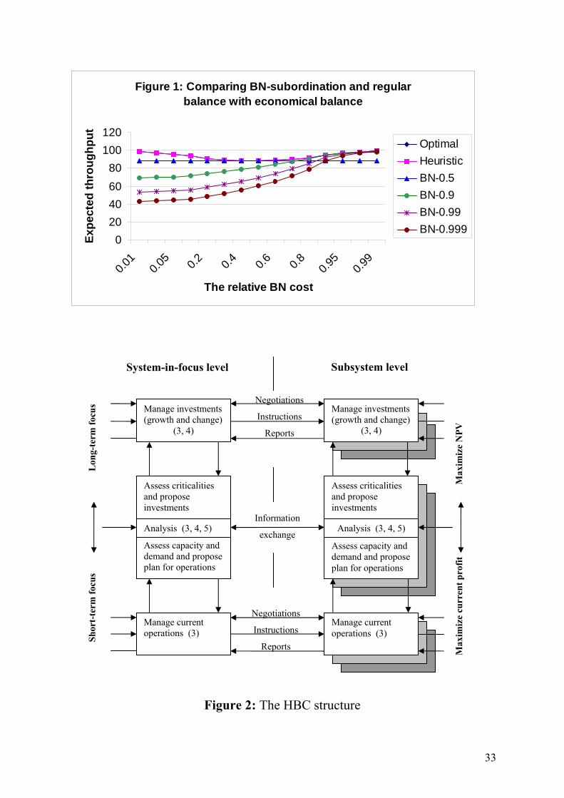
Figure 1: Comparing BN-subordination and regular balance with economical balance

020406080

100120

0.01

0.05 0.2 0.4 0.6 0.8 0.9

50.9

9

The relative BN cost

Expe

cted

thro

ughp

ut

OptimalHeuristicBN-0.5BN-0.9BN-0.99BN-0.999

Shor

t-te

rm fo

cus

L

ong-

term

focu

s

Max

imiz

e cu

rren

t pro

fit

M

axim

ize

NPV

Assess capacity anddemand and Assess capac

propose ity and

demand and propose Assess capacity

Assess capacity and demand and propose plan for operations

Manage investments (growth and change)

(3, 4)

Assess criticalities and propose investments

Assess capacity and demand and propose plan for operations

Manage current operations (3)

Manage investments (growth and change)

(3, 4)

Manage current operations (3)

Analysis (3, 4, 5) Analysis (3, 4, 5)

Assess criticalities and propose investments

Information

exchange

Negotiations

Instructions

Reports

Subsystem level System-in-focus level

Negotiations

Instructions

Reports

Figure 2: The HBC structure

33